f-Uniform Ergodicity of Markov Chains Supervised Project University of Toronto Summer 2006 Supervisor: Professor Jeffrey S. Rosenthal 1 Author: Olga Chilina 2 1 Department of Statistics, University of Toronto, Toronto, Ontario, Canada M5S3G3. Email: jeff@math.toronto.edy. Web: http://probability.ca/jeff/ 2 Department of Statistics, University of Toronto, Toronto, Ontario, Canada M5S3G3. Email: [email protected] 1

Welcome message from author
This document is posted to help you gain knowledge. Please leave a comment to let me know what you think about it! Share it to your friends and learn new things together.
Transcript
f-Uniform Ergodicity of Markov Chains
Supervised Project
University of Toronto
Summer 2006
Supervisor: Professor Jeffrey S. Rosenthal 1
Author: Olga Chilina 2
1Department of Statistics, University of Toronto, Toronto, Ontario, Canada M5S3G3.
Email: [email protected]. Web: http://probability.ca/jeff/2Department of Statistics, University of Toronto, Toronto, Ontario, Canada M5S3G3.
Email: [email protected]
1

Preface
The present project is devoted to the discussion of properties of f -uniform
ergodicity for homogeneous Markov chains. This topic is considered in many
scientific articles (see, for example, [1], [2], [3], [4]). One of the effective tools
that are used to prove properties of Markov chains ergodicity is the coupling
method. The details of this method are shown, for instance, in [1], [3].
The main goal of the current project is a detailed discussion of the cou-
pling method and illustration of its application to the study of ergodic prop-
erties of Markov chains. Moreover, in the project we shall describe useful
conditions for a Markov chain which are sure to be satisfied in case of the
chain’s f -uniform ergodicity.
The project consists of three sections and Appendix. In section 1 (Intro-
duction) we give necessary definitions and notations related to the correct
definition of a homogeneous Markov chain and corresponding measure and
expectation. In particular, we shall state one of the most important theo-
rems related to the current topic, namely, Kolmogorov’s Theorem about a
consistent family of measures.
Since the main interest in studying of Markov chains is represented by
those state spaces (X ,B) which have a countably generated σ-algebra B, it’s
natural to ask a question about the topological construction of such state
spaces. It’s also related to the fact that the main Kolmogorov’s Theorem
holds only in the particular class of topological spaces. This class consists
of complete separable metric topological spaces and is big enough to satisfy
scientific demands in use of Markov chains. The Appendix is devoted to
the description of wonderful relationship between a countably generated σ-
algebra B and a complete separable metric state space X .
In section 2 (Quantative Bounds on Convergence of Time-Homogeneous
Markov Chains) we give a detailed description of the coupling method moti-
vated in the article [3]. This method is used to estimate f -norm that we are
interested in, namely, ||ξP n−ξ′P n||f , where ξ, ξ′ are probability measures on
2
B and P (x,A) is a transition function that defines a homogeneous Markov
chain.
In conclusion, section 3 (f -Uniform Ergodicity of Markov Chains) is de-
voted to the discussion of the properties of f -uniform ergodicity for homo-
geneous Markov chains. Here, on the one hand, we illustrate the application
of the coupling method to the solution of f -uniform ergodicity problem, on
the other hand, we discuss necessary conditions for f -uniform ergodicity of
a homogeneous Markov chain.
3
Contents
1 Introduction 5
1.1 Product of Measurable Spaces . . . . . . . . . . . . . . . . . . 5
1.2 Kolmogorov’s Theorem . . . . . . . . . . . . . . . . . . . . . . 6
1.3 Definition of Markov Chain . . . . . . . . . . . . . . . . . . . 8
2 Quantative Bounds on Convergence of Time-Homogeneous
Markov Chains 10
2.1 Constructions . . . . . . . . . . . . . . . . . . . . . . . . . . . 10
2.2 An Auxiliary Lemma . . . . . . . . . . . . . . . . . . . . . . . 16
2.2.1 A Useful Property of Expectations . . . . . . . . . . . 17
2.2.2 Proof of the Lemma . . . . . . . . . . . . . . . . . . . 19
2.3 Main Time-Homogeneous Result . . . . . . . . . . . . . . . . . 25
3 f-Uniform Ergodicity of Markov Chains 32
3.1 Sufficient Conditions of f -Uniform Ergodicity for Homoge-
neous Markov Chains . . . . . . . . . . . . . . . . . . . . . . . 34
3.2 Necessary Conditions of f -Uniform Ergodicity for Homoge-
neous Markov Chains . . . . . . . . . . . . . . . . . . . . . . . 39
4 Appendix: The Topological Structure of the State Space for
Time-Homogeneous Markov Chains 46
4
1 Introduction
1.1 Product of Measurable Spaces
To understand the theory of Markov chains it is necessary to discuss the
products of measurable spaces (see, for example,[5], pages 144-151).
Let (Ω0,A0), ...(Ωn,An) be fixed sets Ωi with σ-algebras Ai, i = 0, n.
Consider the direct product
n∏
i=0
Ωi =xin
i=0 : xi ∈ Ωi, i = 0, n
The sets of the form A0 × ... × An =xn
i=0 : xi ∈ Ai ∈ Ai, i = 0, n
are
called measurable (n + 1)-rectangulars.
Let A0 be the collection of all finite unions of measurable n-rectangulars.
We can easily check the following lemma:
Lemma 1.1.1. A0 is an algebra of subsets from∏n
i=0 Ωi.
Let’s denote by A the smallest σ-algebra containing A0.
Definition 1.1.2. A is called a direct product of σ-algebras Ai, and we
write A = A0 ⊗ ...⊗An.
Examples.
1. Let Ωi = R = (−∞,∞) and Ai = B(R) be a Borel σ-algebra in R.
Then it’s known (see [5], page 144) that
A0 ⊗ ...⊗An = B(R)⊗ ...⊗ B(R)
is a Borel σ-algebra B(Rn+1) in Rn+1 = R× ...×R︸ ︷︷ ︸n+1
.
2. Let Ωi = X , where X is a countable set, and Ai = A be a σ-algebra
of all subsets in X . Then Ω0 × ... × Ωn = X n+1 is countable, and
A⊗ ...⊗A︸ ︷︷ ︸n+1
is a σ-algebra of all subsets in X n+1 (since xini=0 ∈
A⊗ ...⊗A︸ ︷︷ ︸n+1
∀xini=0 ∈ X n+1, and X n+1 is countable).
5
Now consider a countable collection (Ωi,Ai), i = 0, 1, 2, ..., of measurable
spaces. Let∞∏
i=0
Ωi = xi∞i=0 : xi ∈ Ωi, i = 0, 1, 2, ... .
(In particular, if Ωi = Ω ∀i = 0, 1, 2, ..., then∏∞
i=0 Ωi := Ω∞ = xi∞i=0 : xi ∈ Ω, i = 0, 1, 2, ....)Let Aik ∈ Aik , k = 1, n. The set of the form
C(Ai1 × ...× Aik) =
xi∞i=0 ∈
∞∏
i=0
Ωi : xik ∈ Aik , k = 1, n
is called a cylinder of order n with a base Ai1 × ...× Ain . We shall write
C(Ai1 × ...× Aik) =n∏
k=1
Aik ×∏
i6=ik
Ωi.
Let F be the smallest σ-algebra of subsets in∏∞
i=0 Ωi, containing all
cylinders. Then F is called a direct product of σ-algebras Ai, and we write
F =⊗∞
i=1Ai, and the pair (∏∞
i=1 Ωi,⊗∞
i=1Ai) is called a direct product of
measurable spaces (Ωi,Ai).
Examples.
1. If Ωi = R, Ai = B(R), then (see [5], page 146) the σ-algebra⊗∞
i=0 B(R)
in R∞ is called a Borel σ-algebra in R∞.
2. Let Ωi = X , where X is a countable set, and Ai = F be a σ-algebra of
all subsets in X . Then⊗∞
i=0Ai is not the same as the σ-algebra of all
subsets in X∞.
1.2 Kolmogorov’s Theorem
Let’s consider a particular case of the direct product of measurable spaces,
(R∞,⊗∞
i=0 B(R)). Let P be a probability measure on (R∞,⊗∞
i=0 B(R)). For
each (n + 1)-rectangular A1 × ...× An ∈ B(Rn+1) let
Pn(A0 × ...× An) = P (C(A0 × ...× An)) = P
A0 × ...× An ×
∞∏
i=n+1
R
.
6

Then Pn can be extended to a countably additive probability measure on⊗n
i=0 B(R), and
Pn+1(A0 × ...× An ×R) = Pn(A0 × ...×An) (1)
The equality (1) is called the property of consistency of a sequence of
probability measures Pn defined on⊗∞
i=0 B(R). The following important
theorem takes place:
Theorem 1.2.1. Kolmogorov’s Theorem. Let P1, P2, ..., Pn be a se-
quence of probability measures, defined on (R,B(R)), (R2,B(R2)),..., (Rn,B(Rn)),
respectively, such that the consistency property (1) is satisfied. Then there
exists a unique probability measure P on⊗∞
i=0 B(R) such that
P (C(A0 × ...× An)) = Pn(A0 × ...× An)
for all A0 × ...× An ∈ B(Rn).
The Kolmogorov’s theorem holds even for more general situation (see
remarks in [5], page 168), namely, the following theorem also takes place:
Theorem 1.2.2. Let Ωi be a complete separable metric space, Ai =
B(Ωi) be a σ-algebra of Borel subsets in Ωi, i = 0, 1, 2, .... Let P1, P2, ..., Pn, ...
be a sequence of probability measures defined on (Ω0,A0), (Ω0 × Ω1,A0 ⊗A1),...,(
∏ni=0 Ωi,
⊗ni=0Ai),..., respectively, such that the following consistency
property is satisfied:
Pn+1(A0 × ...× An × Ωn+1) = Pn(A0 × ...× An)
for all Ai ∈ Ai, i = 0, n. Then there exists a unique probability measure P
on (∏∞
i=0 Ωi,⊗∞
i=0Ai) such that
P (C(A0 × ...× An)) = Pn(A0 × ...× An)
for all Ai ∈ Ai, i = 0, n.
Remark 1. As an example of a complete separable metric space we can
consider a countable set X with a discrete metric measure
ρ(x, y) =
1 if x 6= y
0 if x = y
7

In this case, any subset from X is open or closed. Thus, B(X ) is a σ-algebra
of all subsets.
Remark 2. Consider Z = X ×X ×0, 1, where X is countable or finite.
Then Z is countable or finite, and Z is a complete separable metric space
with respect to a discrete metric measure, and B(Z). Thus, theorem 1.2.2 is
true for Ωi = X , Ai = B(X ) and for Ωi = Z, Ai = B(Z), i = 0, 1, 2, ....
Now, keeping in mind considered constructions let’s define a homogeneous
Markov chain.
1.3 Definition of Markov Chain
Let (Ω,F , P ) be a probability space, X0, X1, ..., Xn, ... be a sequence of ran-
dom variables on (Ω,F , P ) with values from some measurable space (S, E),
i.e. Xi : Ω → S and X−1i (B) ∈ F ∀B ∈ E , i = 0, 1, 2, ..., where E is a σ-
algebra of subsets in S. Let Fn = Fn(X0, ..., Xn) be the smallest σ-subalgebra
in A, with respect to which X0, ..., Xn are measurable.
Definition 1.3.1. We say that a sequence X0, X1, ..., Xn, ... forms a
Markov chain , if for all n ≥ m ≥ 0 and for all B ∈ E we have
P (Xn ∈ B|Fm) = P (Xn ∈ B|Xm).
An important role in studying Markov chains is played by transition ker-
nels Pn(x,B), where x ∈ S, B ∈ E such that:
1. When B ∈ E is fixed Pn(x, B) is a measurable function on (S, E);
2. When x ∈ S is fixed Pn(x,B) is a probability measure on (S, E).
It is known (see [5], page 565) that there exists Pn+1(x,B) such that
P (Xn+1 ∈ B|Xn) = Pn+1(Xn, B)
for all B ∈ E , n = 0, 1, 2, ....
If Pn+1(x,B) = Pn(x,B), n = 1, 2, ..., then a Markov chain is called
homogeneous , in this case, P (x,B) = P1(x,B), and P (x,B) is called a
transition kernel for a chain X0, X1, ..., Xn, ....
8
Together with P (x,B) for a Markov chain X0, X1, ..., Xn, ... it’s important
to consider an initial distribution π which is a probability measure on (S, E)
such that π(B) = P (X0 ∈ B).
The pair (π, P (x,B)) completely defines a Markov chain X0, X1, ..., Xn, ...,
since for all Xini=0
P ((X0, ..., Xn) ∈ A) =∫
S
π(dx0)∫
S
P (x0, dx1) · · ·∫
S
IA(x0, ..., xn)P (xn−1, dxn), (2)
where IA is an indicator function, i.e.
IA(x) =
1 if x ∈ A
0 if x /∈ A
and A ∈ ⊗ni=0 E , where
⊗ni=0 E is a direct product of σ-algebras E , i.e. here
we consider (∏n
i=0 S,⊗n
i=0 E).
Using (2) it may be shown that for any bounded measurable non-negative
function g : (∏n
i=0 S,⊗n
i=0 E) → (R,B(R)) the expected value of this function
can be calculated by the following formula
Eg(X0, X1, ..., Xn) =∫
E
π(dx0)∫
E
P (x0, dx1) · · ·∫
E
g(x0, x1, ..., xn)P (xn−1, dxn) (3)
Since for studying Markov chains the initial probability space (Ω,F , P )
is not as important as a measurable space of values (S, E), and an initial
distribution π, and a transition kernel P (x,B), that allow us to calculate
all necessary probability characteristics for the chain with the help of the
formulas (2)and (3), then the chain Xi∞i=0 can be constructed as follows.
Let us have (S, E), π, P (x,B). Consider the product of spaces Ω =∏∞
i=0 S, F =⊗∞
i=0 E . For any A ∈ ⊗ni=0 E let
Pn+1(A) =∫
S
π(dx0)∫
S
P (x0, dx1) · · ·∫
S
IA(x0, ..., xn)P (xn−1, dxn),
using (2).
Thus, we get a consentient sequence of probability measures Pn∞n=0.
Let’s assume that S is a complete separable metric space, and E = B(S).
9
According to theorem 1.2.2, there exists a unique probability measure P on
(∏∞
i=0 S,⊗∞
i=0 E) such that
P (C(A0 × ...× An)) = Pn+1(A0 × ...× An) (4)
for all Ai ∈ E , i = 0, n.
Let Ω =∏∞
i=0 E, F =⊗∞
i=0 E and P be the previous measure on F . Then
for P the equality (2) is satisfied. Consider random variables Yi(xi∞i=0) =
xi ∈ S, xi∞i=0 ∈∏∞
i=0 S, xi ∈ S for all i. Thus,
Yi : (∞∏
i=0
S,∞⊗
i=0
E) = (Ω,F) → (S, E)
.
Theorem 1.3.2 (see [5], pages 566-567) The sequence Yi∞i=0 forms a
homogeneous Markov chain with values from (S, E), initial distribution π and
a transition kernel P (x,B).
Thus, by theorem 1.3.2, we always can say that the chain Xi∞i=0 is
constructed similarly to the way the chain Yi∞i=0 was constructed.
2 Quantative Bounds on Convergence of Time-
Homogeneous Markov Chains
In this section, following the article ”Quantative Bounds on Convergence of
Time-Inhomogeneous Markov Chains” by R. Douc, E. Moulines, and Jeffrey
S. Rosenthal (see [3]), we shall give a detailed description of the coupling
method and its application to the estimation of the f -norm ||ξP n − ξ′P n||f ,where ξ, ξ′ are probability measures on σ-algebra of the chain’s state set, for
a homogeneous Markov chain with a transition function P (x,A).
2.1 Constructions
Let us be given a homogeneous Markov chain X = X0, X1, ..., Xn, ... with a
state space (X ,B(X )), initial distribution π, and transition kernel P (x,B),
10
x ∈ X , B ∈ B(X ), where B(X ) is a σ-algebra of all subsets in X .
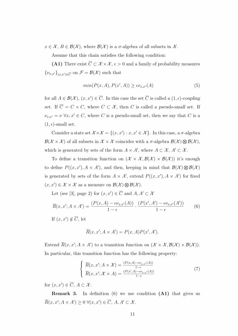
Assume that this chain satisfies the following condition:
(A1) There exist C ⊂ X ×X , ε > 0 and a family of probability measures
νx,x′(x,x′)∈C on F = B(X ) such that
min(P (x,A), P (x′, A)) ≥ ενx,x′(A) (5)
for all A ∈ B(X ), (x, x′) ∈ C. In this case the set C is called a (1, ε)-coupling
set. If C = C × C, where C ⊂ X , then C is called a pseudo-small set. If
νx,x′ = ν ∀x, x′ ∈ C, where C is a pseudo-small set, then we say that C is a
(1, ε)-small set.
Consider a state set X×X = (x, x′) : x, x′ ∈ X. In this case, a σ-algebra
B(X ×X ) of all subsets in X ×X coincides with a σ-algebra B(X )⊗B(X ),
which is generated by sets of the form A× A′, where A ⊂ X , A′ ⊂ X .
To define a transition function on (X × X ,B(X ) × B(X )) it’s enough
to define P ((x, x′), A × A′), and then, keeping in mind that B(X )⊗B(X )
is generated by sets of the form A × A′, extend P ((x, x′), A × A′) for fixed
(x, x′) ∈ X × X as a measure on B(X )⊗B(X ).
Let (see [3], page 2) for (x, x′) ∈ C and A,A′ ⊂ X
R(x, x′; A× A′) =(P (x,A)− ενx,x′(A))
1− ε· (P (x′, A′)− ενx,x′(A
′))1− ε
(6)
If (x, x′) /∈ C, let
R(x, x′; A× A′) = P (x,A)P (x′, A′).
Extend R(x, x′; A× A′) to a transition function on (X × X ,B(X )× B(X )).
In particular, this transition function has the following property:
R(x, x′; A×X ) =(P (x,A)−ενx,x′ (A))
1−ε
R(x, x′;X × A) =(P (x′,A)−ενx,x′ (A))
1−ε
(7)
for (x, x′) ∈ C, A ⊂ X .
Remark 3. In definition (6) we use condition (A1) that gives us
R(x, x′; A× A′) ≥ 0 ∀(x, x′) ∈ C, A,A′ ⊂ X .
11
Let R(x, x′; D) be any transition function on (X × X ,B(X × X ) that
satisfies (7). Above (see (6)) we showed that such functions R(x, x′; D),
where (x, x′) ∈ X × X , D ⊂ X × X , exist.
Let P (x, x′; D) be another transition function on (X ×X ,B(X ×X ) such
that for (x, x′) ∈ C, A,A′ ∈ B(X ) we have
P (x, x′; A× A′) = (1− ε)R(x, x′; A× A′) + ενx,x′(A⋂
A′), (8)
and for (x, x′) /∈ C, A ∈ B(X ) we have
P (x, x′; A×X ) = P (x,A) and P (x, x′;X × A) = P (x′, A)
Remark 4. Such transition functions P (x, x′; D) exist. It’s sufficient
to take P (x, x′; A × A′) = P (x,A)P (x′, A′) for (x, x′) /∈ C, and to take
P (x, x′; A× A′) as in (8) for (x, x′) ∈ C.
Note that P (x, x′; A × A′) = P (x,A)P (x′, A′) for fixed x, x′ ∈ X can be
extended to the “area” on B(X )⊗B(X ), and the area of the rectangle A×A′
is equal to the product of side measures, P (x,A)P (x′, A′).
So, we have an initial transition function P (x,A) on (X ,B(X )), and two
transition functions R(x, x′; D), P (x, x′; D) on (X ×X ,B(X )×B(X )) satis-
fying (7) and (8) respectively.
Following [3], let’s construct now a Markov chain Zn with values from
X × X × 0, 1 = Z. We can write Zn = (Xn, X′n, dn), where Xn, X
′n are
functions with values from X , and dn is a function with values from 0, 1.The cylinders in Z are sets of the form A×A′×0 and A×A′×1, where
A,A′ ∈ B(X ).
To define a Markov chain Zn let’s define a transition function on B(Z) =
B(X )⊗B(X )
⊗B(0, 1) as follows (it’s enough to define for (x, x′, d) ∈ Z
12

and cylinders A× A′ × 0; A× A′ × 1, A,A′ ⊂ X ):
P ((x, x′, d); D) =
P (x,A) if d = 1 and X = X ′ and D = A× A′ × 10 if d = 1 and D = A× A′ × 0ενx,x′(A
⋂A′) if d = 0, (x, x′) ∈ C, D = A× A′ × 1
(1− ε)R(x, x′; A× A′) if d = 0, (x, x′) ∈ C, D = A× A′ × 00 if d = 0, (x, x′) /∈ C, D = A× A′ × 1P (x, x′; A× A′) if d = 0, (x, x′) /∈ C, D = A× A′ × 0
(9)
Let ξ, ξ′ be probability measures on B(X ), δ0 be the Dirac measure on
0, 1 centered on d = 0, i.e. δ0(0) = 1, δ0(1) = 0.
Consider a product of measures µ = ξ ⊗ ξ′ ⊗ δ0 on B(X ) ⊗ B(X ) ⊗B(0, 1) = B(Z). The probability measure µ will be considered as an initial
distribution for Zn∞n=0. Thus, we shall consider a homogeneous Markov
chain defined by the pair (µ, P ) on (Z,B(Z)).
We shall need the following
Proposition 2.1.1.
Pξ⊗ξ′⊗δ0(Zn ∈ A×X × 0, 1) = (ξP n)(A) (10)
Pξ⊗ξ′⊗δ0(Zn ∈ X × A′ × 0, 1) = (ξ′P n)(A′) (11)
(Here Pξ⊗ξ′⊗δ0 is a probability measure on(ZN,
⊗∞n=0 B(Z)
)generated by
the pair (ξ ⊗ ξ′ ⊗ δ0, P ) (see(2)).)
Recall that (ξP )(A) =∫X
P (x,A)ξ(dx), A ⊂ X , and P n = PP n−1, where
(PQ)(x,A) =∫X
P (x, dy)Q(y, A).
Proof of Proposition 2.1.1:
Let n = 0, then using (2) we’ll get that
Pξ⊗ξ′⊗δ0(Z0 = (X0, X′0, d0) ∈ A×X × 0, 1) =
∫
ZIA×X×0,1ξ ⊗ ξ′ ⊗ δ0(d(x0, x
′0, d0))
= ξ ⊗ ξ′ ⊗ δ0(A×X × 0, 1)= ξ(A) · ξ′(X ) · δ0(0, 1)= ξ(A) · 1 · 1 = ξ(A)
13

= (ξ · P 0)(A)
(since, by definition, P 0(x,A) ≡ 1)
Let n = 1. In formula (2) the role of the argument xi is played by the
triple (xi, x′i, di). We have
(Z1 ∈ A×X × 0, 1) = (Z0 ∈ Z; Z1 ∈ A×X × 0, 1)= ((Z0, Z1) ∈ Z × (A×X × 0.1)) ;
IZ×(A×X×0,1)(x0, x′0, d0; x1, x
′1, d1) ≡ IA×X×0,1(x1, x
′1, d1).
According to the formula (2), we get that
Pξ⊗ξ′⊗δ0(Z1 ∈ A×X × 0, 1) = Pξ⊗ξ′⊗δ0 ((Z0, Z1) ∈ Z × (A×X × 0, 1))
=∫
Zξ ⊗ ξ′ ⊗ δ0(d(x0, x
′0, d0))
∫
ZIA×X×0,1(x1, x
′1, d1)P (x0, x
′0, d0; d(x1, x
′1, d
′1))
=∫
Zξ ⊗ ξ′ ⊗ δ0(d(x0, x
′0, d0)) · P (x0, x
′0, d0; A×X × 0, 1)
¿From (9) we have that P ((x0, x′0, d0); A×X × 0, 1) =
=
P (x0, A) if d = 1
ενx0,x′0(A⋂X ) + (1− ε)R(x0, x
′0; A×X ) if d = 0 and (x0, x
′0) ∈ C
P (x0, x′0; A×X ) if d = 0 and (x0, x
′0) /∈ C
=
P (x0, A) if d = 1
ενx0,x′0(A) + P (x0, A)− ενx0,x′0(A) if d = 0 and (x0, x′0) ∈ C
P (x0, A) if d = 0 and (x0, x′0) /∈ C
=
P (x0, A) if d = 1
P (x0, A) if d = 0 and (x0, x′0) ∈ C
P (x0, A) if d = 0 and (x0, x′0) /∈ C
Thus, P ((x0, x′0, d0); A×X × 0, 1) = P (x0, A), and therefore
Pξ⊗ξ′⊗δ0(Z1 ∈ A×X × 0, 1) =∫
Zξ ⊗ ξ′ ⊗ δ0(d(x0, x
′0, d0))P (x0, A)
14

=∫
0,1δ0(d(d0))
∫
Xξ′(dx′0)
∫
Xξ(dx0)P (x0, A)
(by Fubini Theorem)
= (ξ · P )(A)∫
0,1δ0(d(d0))
∫
Xξ′d(x′0)
= (ξ · P )(A)δ0(0, 1)ξ′(X ) = (ξ · P )(A)
Now, let’s show that (10) is true for any n.
We have that
(Zn ∈ A×X × 0, 1) = (Z0 ∈ Z, ..., Zn−1 ∈ Z; Zn ∈ A×X × 0, 1)
=
(Z0, ..., Zn) ∈ Z × ...×Z︸ ︷︷ ︸
n
×(A×X × 0, 1) ;
IZ×...×Z×(A×X×0,1)(x0, x′0, d0; x1, x
′1, d1, ..., xn, x
′n, dn) ≡ IA×X×0,1(xn, x
′n, dn).
By the formula (2), we have that Pξ⊗ξ′⊗δ0(Zn ∈ A×X × 0, 1) =
=∫
Zξ ⊗ ξ′ ⊗ δ0(d(x0, x
′0, d0)) · · ·
∫
ZIA×X×0,1(xn, x
′n, dn)P (xn−1, x
′n−1, dn−1; d(xn, x
′n, dn))
=∫
Zξ ⊗ ξ′ ⊗ δ0(d(x0, x
′0, d0)) · · ·
∫
ZP (xn−2, x
′n−2, dn−2; d(xn−1, x
′n−1, dn−1)) ·
· P (xn−1, x′n−1, dn−1; A×X × 0, 1)
Like we did above, we can show that
P (xn−1, x′n−1, dn−1; A×X × 0, 1) = P (xn−1, A) for all fixed A ∈ B(X ).
And, since from (9) for D = B ×X × 0, 1 we also have that
P (xn−2, x′n−2, dn−2; D) = P (xn−2, B) for all B ∈ B(X ),
then for any bounded function g on X it follows that
∫
X×X×0,1g(xn−1)P (xn−2, x
′n−2, dn−2; d(xn−1, x
′n−1, dn−1)) =
∫
Xg(xn−1)P (xn−2, dxn−1)
(since the intergrand depends only on xn−1, i.e.
g(xn−1) = g(xn−1) · 1(x′n−1) · 1(dn−1),
15

where 1(x′n−1) ≡ 1 ≡ 1(dn−1) and the integration with respect to xn−1 and
dn−1 gives us the indentity.)
Hence,
∫
ZP (xn−2, x
′n−2, dn−2; d(xn−1, x
′n−1, dn−1))P (xn−1, A) = (taking g(xn−1) = P (xn−1, A))
=∫
XP (xn−1, A)P (xn−2, dxn−1)
= P 2(xn−2, A)
If we keep going in the same direction, we shall get that
Pξ⊗ξ′⊗δ0(Zn ∈ A×X × 0, 1) =
=∫
Zξ ⊗ ξ′ ⊗ δ0(d(x0, x
′0, d0)) ·
∫
ZP (x0, x
′0, d0; d(x0, x
′0, d0)) · P n−1(x1, A)
=∫
Zξ ⊗ ξ′ ⊗ δ0(d(x0, x
′0, d0)) · P n(x0, A)
=∫
XP n(x0, A)ξ(dx0) ·
∫
Xξ′(dx′0) ·
∫
0,1δ0(d(d0))
(by Fubini Theorem)
= (ξ · P n)(A).
Similarly, we can prove (11).
2
2.2 An Auxiliary Lemma
Again following [3], denote by P ∗ a Markov kernel defined for (x, x′) ∈ X×X ,
A ∈ B(X × X ) by formula
P ∗(x, x′; A) =
P (x, x′, A) if (x, x′) /∈ C
R(x, x′, A) if (x, x′) ∈ C
For a probability measure µ on B(X×X ) denote by P ∗µ and E∗
µ a probabil-
ity and expectation, respectively, on( ∏∞
n=0X ×X ,⊗∞
n=0 B(X ×X ))
induced
by µ and P ∗ according to formulas (2) and (3).
16
Lemma. Let (A1) hold (thus, P , R are defined). Then for any n ≥ 0
and any non-negative Borel function φ : (X × X )n+1 → R+ the following
equality holds:
Eξ⊗ξ′⊗δ0φ(X0, X′0, ..., Xn, X
′n) · Idn=0 = E∗
ξ⊗ξ′φ(X0, X′0, ..., Xn, X
′n)(1− ε)Nn−1(12)
where Ni =∑i
j=0 IC(Xj, X′j), N−1 := 0, and
Idn=0(X0, X′0, d0; ...; Xn, X ′
n, dn) =
1 if dn = 0
0 if dn 6= 0
Before we prove this lemma let us discuss some facts from the measure
theory.
2.2.1 A Useful Property of Expectations
Let X be a set, F be a σ-algebra of subsets from X , and P1, P2 be two
probability measures on F . Let’s give one sufficient condition for the equality
P1(A) = P2(A) for all A ∈ F , and, thus, for the equality∫X
fdP1 =∫X
fdP2 for
any non-negative measurable function f : (X ,F) → (R,B(R)), where B(R)
is a Borel σ-algebra (i.e. f−1(B) ∈ F ∀B ∈ B(R); such functions are called
Borel functions).
Definition 2.2.1.1. A system N of subsets from X is called a semiring,
if
1. ∅ ∈ N ;
2. A ∩B ∈ N , if A,B ∈ N ;
3. If A1 ⊂ A, A1, A ∈ N , then we can represent A as a union, i.e. A =⋃n
i=1 Ai, Ai ∈ N , Ai ∩ Aj = ∅, i 6= j, i, j = 1, n.
Examples of Semirings:
1. N = (a, b), [a, b], [a, b), (a, b] : a ≤ b, a, b ∈ R is a semiring of subsets
in R;
17
2. (Important for us) Let (X ,F) be a given set with a fixed σ-algebra.
Consider Y =∏n
i=0X and let N = ∏n
i=0 Ai : Ai ∈ F
be a system
of all n-parallelepipeds in Y . Clear that ∅ =∏n
i=0 ∅ ∈ N . If F1 =∏n
i=0 Ai ∈ N , F2 =∏n
i=0 Bi ∈ N , then F1∩F2 =∏n
i=0 Ai∩Bi ∈ N . Let
F =∏n
i=0 Ai ∈ N and F1 =∏n
i=0 Bi ∈ N , F1 ⊂ F . Hence, Bi ⊂ Ai,
i = 0, n. Take F2 = (A0 \B0)×B1 × ...×Bn ∈ N . Then F1 ∩ F2 = ∅,F1∪F2 = A0×B1×...×Bn. Now, let F3 = A0×(A1\B1)×B2×...×Bn ⇒F3 ∈ N , F3 ∩ Fi = ∅, i = 1, 2, F1 ∪ F2 ∪ F3 = A0 ×A1 ×B2 × ...×Bn.
Continuing we construct F2, ..., Fn+1 ∈ N such that Fi ∪ Fj = ∅, i 6= j
and⋃n+1
i=1 Fi = F . Hence, N is a semiring.
Now let’s introduce well-known properties of semirings.
Lemma 2.2.1.2.If N is a semiring, A1, ..., An, A ∈ N , Ai ⊂ A, Ai∩Aj =
∅, i 6= j, i, j = 1, n, then there exist An+1, ..., Ak ∈ N such that A =⋃k
i=1 Ai.
Lemma 2.2.1.3. If N is a semiring, A1, ..., An ∈ N , then there exist
B1, ..., Bk ∈ N such that Bi ∩ Bj = ∅, i 6= j, i, j = 1, k and Ai =⋃n(i)
j=1 Bsj
for some s1 < ... < sn(i) and all i = 1, n.
Lemma 2.2.1.4. The smallest algebra of sets A(N ) containing a semir-
ing N with an identity X ∈ N consists of the sets of the form A =⋃n
k=1 Ak,
where Ak ∈ N , k = 1, n, n ∈ N.
¿From this lemma it follows that
Lemma 2.2.1.5. Any set A ∈ A(N ) can be represented as A =⋃k
i=1 Bi,
where Bi ∈ N , Bi ∩Bj = ∅, i 6= j, i, j = 1, k.
Let F be the smallest σ-algebra generated by a semiring N with identity
X , i.e. F is generated by algebra A(N ).
Theorem 2.2.1.6. If µ is a σ-finite measure on algebra A(N ), then
there exists a unique measure µ′ on algebra F , for which µ′(A) = µ(A) for
any A ∈ A(N ).
¿From this theorem we get what we wanted:
Theorem 2.2.1.7. If P1, P2 are two σ-finite measures on F and P1(B) =
P2(B) for any B ∈ N , then P1(A) = P2(A) ∀A ∈ F and∫X
fdP1 =∫X
fdP2
18
for any positive Borel function f : (X ,F) → R.
Proof: From lemma 2.2.1.5 it follows that ∀A ∈ A(N ) A =⋃k
i=1 Bi,
Bi ∈ N , Bi ∩Bj = ∅, i 6= j, i, j = 1, k. Therefore
P1(A) =k∑
i=1
P1(Bi) =k∑
i=1
P2(Bi) = P2(A),
i.e. measures P1 and P2 are equal on A(N ). Hence, by theorem 3.1.6, it
follows that P1(A) = P2(A) ∀A ∈ F , and, thus,∫X
fdP1 =∫X
fdP2 for any
positive Borel function f : (X ,F) → R.
2
Let’s now apply theorem 2.2.1.7 to our case. Let X be a set, B be a
σ-algebra of all subsets in X . Consider Y =∏n
i=0X and A =⊗n
i=0 B.
As we noted earlier (see section 1.1), σ-algebra A is the smallest σ-algebra
containing semiring N of all n-rectangulars A0 × ... × An, Ai ∈ B, i = 0, n
(see example 2 of the previous section).
Thus, we have
Theorem 2.2.1.8. Let P1, P2 be two finite measures on⊗n
i=0 B. If
P1(A0× ...×An) = P2(A0× ...×An) for any Ai ∈ B, i = 0, n, then P1(D) =
P2(D) for any D ∈ ⊗ni=0 B and
EP1(f) =∫
Yf(x1, ..., xn)dP1 =
∫
Yf(x1, ..., xn)dP2 = EP2(f)
for any positive Borel function f : (Y ,⊗n
i=0 B) → R.
Now we can move to the lemma’s proof.
2.2.2 Proof of the Lemma
The expectation E∗ξ⊗ξ′ is constructed by measure P ∗
ξ⊗ξ′ defined by an initial
distribution ξ ⊗ ξ′ given on B(X ×X ), and by a Markov transition function
P ∗(x, x′, A). In particular formula (3) holds for E∗ξ⊗ξ′ , i.e.
E∗ξ⊗ξ′(g(x0, x
′0, ..., xn, x′n)) =
∫
X×Xd(ξ ⊗ ξ′)
∫
X×XP ∗(x0, x
′0; d(x1, x
′1)) · ...
19

... ·∫
X×Xg(x0, x
′0, ..., xn, x′n)P ∗(xn−1, x
′n−1; d(xn, x′n))
(13)
For each A ∈ ⊗ni=0 B(X × X ) let
µ1(A) = E∗ξ⊗ξ′(IA(x0, x
′0, ..., xn, x
′n)(1− ε)Nn−1).
Since 0 ≤ IA · (1 − ε)Nn−1 ≤ 1, then µ1 is a finite countably additive
measure on⊗n
i=0 B(X × X ).
The expectation Eξ⊗ξ′⊗δ0 is constructed by measure Pξ⊗ξ′⊗δ0 defined by an
initial distribution ξ⊗ ξ′⊗ δ0 given on B(Z), where Z = X ×X ×0, 1, and
by a Markov transition function P ((x, x′, d); D) (see (9)), where (x, x′) ∈ X ,
d ∈ 0, 1, D ∈ B(Z). For Eξ⊗ξ′⊗δ0 the formula (3) also holds, i.e.
Eξ⊗ξ′⊗δ0(h(x0, x′0, d0, ..., xn, x′n, dn)) =
∫
Zd(ξ ⊗ ξ′ ⊗ δ0)
∫
ZP (x0, x
′0, d0; d(x1, x
′1, d0)) · ...
... ·∫
Zh(x0, x
′0, d0, ..., xn, x′n, dn)P (xn−1, x
′n−1, dn−1; d(xn, x′n, dn)) (14)
For each A ∈ ⊗ni=0 B(X×X ) consider an integrable function on (Zn,
⊗ni=0 B(Z))
hA(x0, x′0, d0; ...; xn, x′n, dn) = IA(x0, x
′0, ..., xn, x
′n) · Idn=0.
Let µ2(A) = Eξ⊗ξ′⊗δ0(hA(x0, x′0, d0; ...; xn, x′n, dn)).
Since Eξ⊗ξ′⊗δ0 is an expectation, then µ2 is a finite countably additive
measure on⊗n
i=0 B(X×X ). (For example, if A =⋃∞
m=1 Am, where Am∩Ak =
∅, m 6= k, m, k = 1,∞, Am ∈ ⊗ni=0 B(X × X ), then
µ2(∞⋃
m=1
) = Eξ⊗ξ′⊗δ0(h⋃∞
m=1Am
(x0, x′0, d0; ...; xn, x
′n, dn))
= Eξ⊗ξ′⊗δ0(I⋃∞
m=1Am· Idn=0)
= Eξ⊗ξ′⊗δ0
( ∞∑
m=1
IAm · Idn=0)
=∞∑
m=1
Eξ⊗ξ′⊗δ0(IAm · Idn=0)
=∞∑
m=1
µ2(Am).)
20
So, we have two finite measures µ1 and µ2 on⊗n
i=0 B(X ×X ). If we show
that µ1(B0× ...×Bn) = µ2(B0× ...×Bn) for any Bi = Ai×A′i ∈ B(X ×X ),
Ai, A′i ∈ B(X ), i = 0, n, then, by theorem 2.2.1.7, we’ll get that µ1(D) =
µ2(D) ∀D ∈ ⊗ni=0 B(X × X ), since the sets (A × A′
0) × ... × (An × A′n),
Ai, A′i ∈ B(X ) form a semiring in B(X ×X ) = B(X )⊗ B(X ) (can be shown
as in example 2). Therefore for any linear combination h(x1, x′1, ..., xn, x′n) =
∑mi=1 αiIDi
, αi ∈ R, Di ∈ ⊗ni=0 B(X × X ), i = 1,m we have
Eξ⊗ξ′⊗δ0(h(x0, x′0, ..., xn, x
′n)Idn=0) =
m∑
i=1
αiEξ⊗ξ′⊗δ0(IDi· Idn=0)
=m∑
i=1
αiµ2(Di) =m∑
i=1
αiµ1(Di)
=m∑
i=1
αiE∗ξ⊗ξ′(IDi
(1− ε)Nn−1)
= E∗ξ⊗ξ′(h · (1− ε)Nn−1).
Now let φ : (X ×X )n+1 → R+ be any non-negative Borel function. Then
there exists a sequence of step functions hk(x0, x′0, ..., xn, x′n) =
∑m(k)i=1 α
(n)i I
D(n)i
such that 0 ≤ hk ↑ φ ⇒ hk · Idn=0 ↑ φ · Idn=0. Therefore
Eξ⊗ξ′⊗δ0(φ(x0, x′0, ..., xn, x
′n) · Idn=0) = lim
k→∞Eξ⊗ξ′⊗δ0(hk · Idn=0)
= limk→∞
E∗ξ⊗ξ′(hk · (1− ε)Nn−1)
= E∗ξ⊗ξ′(φ(x0, x
′0, ..., xn, x
′n)(1− ε)Nn−1)
Thus, to prove the lemma it’s enough to check the equality
µ1(B0 × ...×Bn) = µ2(B0 × ...×Bn)
for any Bi = Ai × A′i ∈ B(X × X ), Ai, A
′i ∈ B(X ), i = 0, n, or, the equality
E∗ξ⊗ξ′(IB0×...×Bn(1− ε)Nn−1) = Eξ×ξ′×δ0(IB0×...×Bn · Idn=0) (15)
From formula (13) we have that
E∗ξ⊗ξ′(IB0×...×Bn(1− ε)Nn−1) =
∫
X×Xd(ξ ⊗ ξ′) · ...
21

... ·∫
X×XP ∗(xn−2, x
′n−2; d(xn−1, x
′n−1))
∫
X×XIB0×...×Bn(1− ε)Nn−1P ∗(xn−1, x
′n−1; d(xn, x′n))
=∫
X×Xd(ξ ⊗ ξ′) · ... ·
∫
X×XIB0(x0, x
′0) · ... · IBn−1(xn−1, x
′n−1) ·
· (1− ε)Nn−1P ∗(xn−2, x′n−2; d(xn−1, x
′n−1)) ·
∫
X×XIBn(xn, x′n)P ∗(xn−1, x
′n−1; d(xn, x′n))
From the definition of P ∗(x, x′, A) we have that
∫
X×XIBn(xn, x
′n)P ∗(xn−1, x
′n−1; d(xn, x
′n)) = P ∗(xn−1, x
′n−1; Bn)
=
P (xn−1, x′n−1, Bn) if (xn−1, x
′n−1) /∈ C
R(xn−1, x′n−1, Bn) if (xn−1, x
′n−1) ∈ C
Since
(1− ε)Nn−1(x0,x′0,...,xn−1,x′n−1) = (1− ε)Nn−2 · (1− ε)IC
(xn−1,x′n−1)
=
(1− ε)Nn−2+1 if (xn−1, x′n−1) ∈ C,
(1− ε)Nn−2 if (xn−1, x′n−1) /∈ C
then
E∗ξ⊗ξ′(IB0×...×Bn(1− ε)Nn−1) =
∫
X×Xd(ξ ⊗ ξ′) · ... ·
∫
X×XP ∗(xn−3, x
′n−3; d(xn−2, x
′n−2)) ·
·( ∫
C
IB0×...×Bn−1(1− ε)Nn−2+1R(xn−1, x′n−1, Bn)P ∗(xn−2, x
′n−2; d(xn−1, x
′n−1)) +
+∫
Cc
IB0×...×Bn−1(1− ε)Nn−2P (xn−1, x′n−1, Bn)P ∗(xn−2, x
′n−2; d(xn−1, x
′n−1))
)
=∫
X×Xd(ξ ⊗ ξ′) · ... ·
∫
X×XP ∗(xn−3, x
′n−3; d(xn−2, x
′n−2)) ·
·∫
X×XIB0×...×Bn−1
(IC(xn−1, x
′n−1)(1− ε)Nn−1R(xn−1, x
′n−1, Bn) +
+ ICc(xn−1, x
′n−1)(1− ε)Nn−2P (xn−1, xn−1, Bn)
)P ∗(xn−2, x
′n−2; d(xn−1, x
′n−1))
= E∗ξ⊗ξ′
[IB0×...×Bn−1(x0, x
′0, ..., xn−1, x
′n−1)(IC(xn−1, x
′n−1)(1− ε)Nn−1R(xn−1, x
′n−1, Bn) +
+ ICc(xn−1, x
′n−1)(1− ε)Nn−2P (xn−1, x
′n−1, Bn))
](16)
Now let Di = Bi × 0, 1, i = 0, (n− 1), D′n = Bn × 0. We have that
IB0×...×Bn(x0, x′0, ..., xn, x
′n) · Idn=0 = IB0(x0, x
′0) · ... · IBn−1(xn−1, x
′n−1) · IBn(xn, x′n) · Idn=0
22

= IB0(x0, x′0) · I0,1(d0) · ... · IBn−1(xn−1, x
′n−1) · I0,1(dn−1) · IBn×0(xn, x
′n, dn)
= ID0(x0, x′0, d0) · ... · IDn−1(xn−1, x
′n−1, dn−1) · ID′n(xn, x
′n, dn)
= ID0×...×Dn−1×D′n(x0, x′0, d0; ...; xn, x
′n, dn)
Thus, from formula (14) we have that
Eξ⊗ξ′⊗δ0(IB0×...×Bn · Idn=0) =∫
Zd(ξ ⊗ ξ′ ⊗ δ0) · ...
·∫
ZID0(x0, x
′0, d0) · ... · IDn−1(xn−1, x
′n−1, dn−1)P (xn−2, x
′n−2, dn−2; d(xn−1, x
′n−1, dn−1))
·∫
ZID′n(xn, x
′n, dn)P (xn−1, x
′n−1, dn−1; d(xn, x
′n, dn))
From the definition of P (x, x′, d; D) (see (9)) we have that
∫
ZID′n(xn, x′n, dn)P (xn−1, x
′n−1, dn−1; d(xn, x
′n, dn)) =
=∫
ZIAn×A′n×0(xn, x
′n, d)P (xn−1, x
′n−1, dn−1; d(xn, x′n, dn))
= P (xn−1, x′n−1, dn−1; An × A′
n × 0)
=
0 if dn−1 = 1
(1− ε)R(xn−1, x′n−1; An × A′
n) if dn−1 = 0, (xn−1, x′n−1) ∈ C
P (xn−1, x′n−1; An × A′
n) if dn−1 = 0, (xn−1, x′n−1) /∈ C
Thus,
Eξ⊗ξ′⊗δ0(IB0×...×Bn · Idn=0) =∫
Zd(ξ ⊗ ξ′ ⊗ δ0) · ...
·∫
ZID0(x0, x
′0, d0) · ... · IDn−2(xn−2, x
′n−2, dn−2)P (xn−3, x
′n−3, dn−3; d(xn−2, x
′n−2, dn−2)) ·
·∫
ZIDn−1(xn−1, x
′n−1, dn−1)P (xn−2, x
′n−2, dn−2; d(xn−1, x
′n−1, dn−1)) ·
·
0 if dn−1 = 1
(1− ε)R(xn−1, x′n−1; An × A′
n) if dn−1 = 0, (xn−1, x′n−1) ∈ C
P (xn−1, x′n−1; An × A′
n) if dn−1 = 0, (xn−1, x′n−1) /∈ C
= (since D′n−1 = An−1 × A′
n−1 × 0 ) =
=∫
Zd(ξ ⊗ ξ′ ⊗ δ0) · ... ·
∫
ZP (xn−3, x
′n−3, dn−3; d(xn−2, x
′n−2, dn−2)) ·
23

·∫
ZID0×...×Dn−2×D′n−1
(IC(xn−1, x
′n−1)(1− ε)R(xn−1, x
′n−1; An × A′
n) +
+ ICc(xn−1, x
′n−1)P (xn−1, x
′n−1; An × A′
n))dP (xn−2, x
′n−2, dn−2; d(xn−1, x
′n−1, dn−1)
= Eξ⊗ξ′⊗δ0
[IB0×...×Bn−1 · Idn=0
(IC(xn−1, x
′n−1)(1− ε)R(xn−1, x
′n−1; An × A′
n) +
+ ICc(xn−1, x
′n−1)P (xn−1, x
′n−1; An × A′
n))]
(17)
Now using (16), (17) and mathematical induction show that (15) is true
for any Bi = Ai × A′i ∈ B(X × X ), Ai, A
′i ∈ B(X ), i = 0, n. For n = 0 from
N0−1 = N−1 = 0, and (13), (14) we have that
E∗ξ⊗ξ′(IB0) =
∫
X×XIB0d(ξ ⊗ ξ′) = (ξ ⊗ ξ′)(A0 × A′
0) = ξ(A0) · ξ′(A′0);
Eξ⊗ξ′⊗δ0(IB0 · Idn=0) =∫
X×X×0,1IA0(x0) · IA′0(x
′0) · Id0=0d(ξ ⊗ ξ′ ⊗ δ0)
= (by Fubini’s Theorem) = ξ(A0)ξ′(A′
0)δ0(0)= (since δ0(0) = 1) = ξ(A0)ξ
′(A′0),
i.e. (15) is true for n = 0. Let (15) be true for (n− 1), i.e.
Eξ⊗ξ′(IB0×...×Bn−1 · (1− ε)Nn−2) = Eξ⊗ξ′⊗δ0(IB0×...×Bn−1 · Idn−1=0)
for all Bi = Ai × A′i ∈ B(X × X ), Ai, A
′i ∈ B(X ), i = 0, (n− 1), i.e.
µ1(B0 × ...×Bn−1) = µ2(B0 × ...×Bn−1).
Then, as shown above, we have that
E∗ξ⊗ξ′(φ(x0, x
′0, ..., xn−1, x
′n−1) · (1− ε)Nn−2) = Eξ⊗ξ′⊗δ0(φ(x0, x
′0, ..., xn−1, x
′n−1) · Idn−1=0(18)
for any non-negative Borel function φ : (X × X )n−1 → R+. Take
φ(x0, x′0, ..., xn−1, x
′n−1) = IB0×...×Bn−1
(IC(xn−1, x
′n−1)(1− ε)R(xn−1, x
′n−1; An × A′
n) +
+ ICc(xn−1, x
′n−1)P (xn−1, x
′n−1; An × A′
n)).
24

Then from (16), (17) and (18) it follows that
E∗ξ⊗ξ′(IB0×...×Bn · (1− ε)Nn−1) = (by (16) ) = E∗
ξ⊗ξ′
(φ(x0, x
′0, ..., xn−1, x
′n−1)(1− ε)Nn−2
)
= (by (18)) = Eξ⊗ξ′⊗δ0(φ(x0, x′0, ..., xn−1, x
′n−1)Idn−1=0)
= (by (17)) = Eξ⊗ξ′⊗δ0(IB0×...×Bn · Idn=0),
i.e. (15) is true, and this finishes the proof of the lemma.
2
2.3 Main Time-Homogeneous Result
Let X , F = B(X ) be the same as before, ξ, ξ′ be probability measures
on B(X ), and P (x,A), where x ∈ X , A ∈ B(X ), be a Markov transition
function.
For function f : X → [1,∞) define an f -norm of a signed measure µ on
B(X ) by
||µ||f := sup|φ|≤f
|µ(φ)|,
where φ : (X ,B(X )) → R is a Borel function.
If f ≡ 1, then by definition we have
||µ||1 := ||µ||TV ,
where || · ||TV is a total variation norm.
Our goal is to obtain an estimation for f -norms
||ξP n − ξ′P n||f and ||ξP n − ξ′P n||TV
in order to find conditions when these f -norms approach zero.
Lemma 2.3.1. Let f : X → [1,∞) and φ : (X ,B(X )) → R be a Borel
function such that supx∈X|φ(x)|f(x)
< ∞; ξ, ξ′ be probability measures on B(X ),
and P (x,A) be a Markov transition function. Let condition (A1) be satisfied.
Then
|ξP nφ− ξ′P nφ| ≤(
supx∈X
|φ(x)|f(x)
)E∗
ξ⊗ξ′
((f(Xn) + f(X ′
n))(1− ε)Nn−1
)(19)
25

Proof: By Proposition 2.1.1, for any A ∈ B(X ) we have
(ξP n)(A) = Pξ⊗ξ′⊗δ0(Zn ∈ A×X × 0, 1) = (see the proof of Proposition 2.1.1)
=∫
Zd(ξ ⊗ ξ′ ⊗ δ0) · ... ·
∫
ZIA×X×0,1(xn, x
′n, dn)P (xn−1, x
′n−1, dn−1; d(xn, x
′n, dn))
Thus, two finite measures
µ1(A) = (ξP n)(A) and µ2(A) = Pξ⊗ξ′⊗δ0(Zn ∈ A×X × 0, 1)
coincide on σ-algebra B(X ). Hence, the expectations constructed by these
measures also coincide, i.e. for any integrable (with respect to measures µ1
and µ2) Borel function φ : (X ,B(X )) → R we have
(ξP n)(φ) =∫
Xφ(xn)d(ξP n) =
∫
Xφ(xn)dPξ⊗ξ′⊗δ0 = Eξ⊗ξ′⊗δ0(φ(Xn)) (20)
Similarly,
(ξ′P n)(φ) = Eξ⊗ξ′⊗δ0(φ(X ′n)) (21)
By definition, chain Zn was constructed as follows: Z0 = (X0, X′0, d0), and
if we define Zn−1 = (Xn−1, X′n−1, dn−1), n > 1, then for Zn = (Xn, X ′
n, dn)
when dn−1 = 1 we let X ′n = Xn ∼ P (Xn−1), dn = 1, and when dn−1 = 0 we
let
X ′n = Xn = X ∼ νXn,X′
n, dn = 1 if (Xn−1, X
′n−1) ∈ C
(Xn, X′n) ∼ R(Xn−1, X
′n−1), dn = 0 if (Xn−1, X
′n−1) ∈ C
(Xn, X′n) ∼ P (Xn−1, X
′n−1), dn = 0 if (Xn−1, X
′n−1) /∈ C
Thus, it’s always true that Xn = X ′n when dn = 1.
Then it follows that
I0,1(dn) · (φ(Xn)− φ(X ′n)) = (φ(Xn)− φ(X ′
n)) · Idn=0.
Therefore from (20) and (21) we have that
|ξP nφ− ξ′P nφ| = |Eξ⊗ξ′⊗δ0
(φ(Xn)− φ(X ′
n))· Idn=0|
≤ Eξ⊗ξ′⊗δ0
((|φ(Xn)|+ |φ(X ′
n)|) · Idn=0)
≤(since |φ(Xn)| = |φ(Xn(ω))| = |φ(Xn(ω))|·f(Xn(ω))
f(Xn(ω))≤ supx∈X
|φ(x)|f(x)
· f(Xn))
≤ supx∈X
|φ(x)|f(x)
Eξ⊗ξ′⊗δ0
((f(Xn) + f(X ′
n)) · Idn=0)
26

Therefore from the main Lemma (see section 2.2) we obtain that
|ξP nφ− ξ′P nφ| ≤ supx∈X
|φ(x)|f(x)
E∗ξ⊗ξ′
((f(Xn) + f(X ′
n))(1− ε)Nn−1
).
2
Now, consider the following condition for Markov transition function
P ∗(x, x′, A):
(A2) There exist a function V : X × X → [1,∞) and constants b > 0,
λ ∈ (0, 1) such that
P ∗V ≤ λV + bIC (22)
Theorem 2.3.2. Let conditions (A1) and (A2) hold. Let f : X → [1,∞)
be such that f(x) + f(x′) ≤ 2V (x, x′) ∀(x, x′) ∈ X × X . Then for any
j ∈ 1, ..., n + 1 and any initial probability measures ξ and ξ′ on B(X ) the
following inequalities are true:
||ξP n − ξ′P n||TV ≤ 2(1− ε)jIj≤n + 2λnBj−1(ξ ⊗ ξ′)(V ) (23)
||ξP n − ξ′P n||f ≤ 2(1− ε)j(b(1− λ)−1 + λn(ξ ⊗ ξ′)(V )
)Ij≤n + 2λnBj−1(ξ ⊗ ξ′)(V ),
(24)
where B = max(1, (1− ε)λ−1 sup(x,x′)∈C RV (x, x′)
).
Proof: For any j ∈ 1, ..., n + 1 we have
E∗ξ⊗ξ′
[(f(Xn) + f(X ′
n))(1− ε)Nn−1
]=
= (since INn−1≥j + INn−1<j ≡ 1 and Nn−1 ≥ j ∩ Nn−1 < j = ∅)= E∗
ξ⊗ξ′
[(f(Xn) + f(X ′
n))(1− ε)Nn−1INn−1≥j]
+
+ E∗ξ⊗ξ′
[(f(Xn) + f(X ′
n))(1− ε)Nn−1INn−1<j]
≤(since f(Xn) + f(X ′
n) ≤ 2V (Xn, X′n)
)
≤ E∗ξ⊗ξ′
[(f(Xn) + f(X ′
n))(1− ε)Nn−1INn−1≥j]
+
+ 2E∗ξ⊗ξ′
[V (Xn, X
′n)(1− ε)Nn−1INn−1<j
]
(25)
27

Since (1− ε)Nn−1 · INn−1≥j ≤ (1− ε)j · INn−1≥j ≤ (1− ε)j, then
E∗ξ⊗ξ′
[(f(Xn)+ f(X ′
n))(1− ε)Nn−1INn−1≥j]≤ (1− ε)jE∗
ξ⊗ξ′
[f(Xn)+ f(X ′
n)]
If f ≡ 1, then f(Xn) + f(X ′n) = 2 and the first term in inequality (25) is
estimated by number 2(1− ε)j.
Using condition (A2) we have that
(P ∗)nV = (P ∗)n−1(P ∗V )
≤ (P ∗)n−1(λV + bIC) (by (A2))
≤ λ(P ∗)n−1V + b ≤ λ(λ(P ∗)n−2V + b) + b
= λ2(P ∗)n−2V + b(1 + λ) ≤ ... ≤ λnV + bn−1∑
k=0
λk
≤ λnV +b
1− λ(since
∑∞k=0 = 1
1−λ).
Then from the inequality f(x) + f(x′) ≤ 2V (x, x′) and formula (3) for
P ∗(x, x′, A) we have
E∗ξ⊗ξ′
[f(Xn) + f(X ′
n)]≤ 2E∗
ξ⊗ξ′(V )
= 2∫
X×Xd(ξ ⊗ ξ′) · ... ·
∫
X×XV (xn, x
′n)P ∗(xn−1, x
′n−1; d(xn, x
′n))
= 2∫
X×X(P ∗)nV d(ξ ⊗ ξ′) ≤ 2λn
∫
X×XV d(ξ ⊗ ξ′) +
2b
1− λ
= 2λn(ξ ⊗ ξ′)(V ) +2b
1− λ. (26)
By lemma 2.3.1 we have
|ξP nφ− ξ′P nφ| ≤(
supx∈X
|φ(x)|f(x)
)E∗
ξ⊗ξ′
[(f(Xn) + f(X ′
n))(1− ε)Nn−1
].
Thus, (see (25) and (26))
||ξP n − ξ′P n||f = sup|φ|≤f
|ξP nφ− ξ′P nφ| ≤ E∗ξ⊗ξ′
[(f(Xn) + f(X ′
n))(1− ε)Nn−1
]
≤ 2(1− ε)j(b(1− λ)−1 + λn(ξ ⊗ ξ′)(V )
)+ 2E∗
ξ⊗ξ′
[V (Xn, X ′
n)(1− ε)Nn−1 · INn−1<j],
(27)
28

and in the case when f ≡ 1 we have
||ξP n − ξ′P n||TV ≤ 2(1− ε)j + 2E∗ξ⊗ξ′
[V (Xn, X
′n) · (1− ε)Nn−1 · INn−1<j
]
(28)
Note that if j > n, then INn−1≥j = 0, since 0 ≤ Nn−1(x0, x′0, ..., xn−1, x
′n−1) ≤
n. Therefore in this case we don’t have the first term in (25), (27) and (28),
and we can rewrite inequalities (27) and (28) as
||ξP n − ξ′P n||f ≤ 2(1− ε)j(b(1− λ)−1 + λn(ξ ⊗ ξ′)(V )
)· Ij≤n +
+ 2E∗ξ⊗ξ′
[V (Xn, X ′
n)(1− ε)Nn−1 · INn−1<j]
(29)
and
||ξP n − ξ′P n||TV ≤ 2(1− ε)j · Ij≤n + 2E∗ξ⊗ξ′
[V (Xn, X ′
n)(1− ε)Nn−1 · INn−1<j](30)
Now let’s estimate the second term in (29) and (30).
Let B = max(1, (1− ε)λ−1 sup(x,x′)∈C RV (x, x′)
). For each s ≥ 0 define
Ms := λ−sB−Ns−1V (Xs, X′s)(1− ε)Ns−1 ,
and show that Ms, s ≥ 0 is a (F , P ∗ξ⊗ξ′)-supermartingale, where F :=
Fs := σ(Xi, X′i; i ≤ s), s ≥ 0 is a σ-algebra in
⊗∞i=0 B(X ×X ) generated by
σ-subalgebra σ(Xi, X′i; i ≤ s)=(the smallest σ-subalgebra in
⊗∞i=0 B(X ×X )
with respect to which (Xi, X′i) are measurable, i ≤ s).
Note that Fs := σ(Xi, X′i; i ≤ s) ⊂ A ⊗ ∏∞
i=s+1(X×X ) : A ∈ ⊗si=0 B(X×
X ).Now we shall need the following theorem from homogeneous Markov
chains theory:
Theorem 2.3.3. Let Yn∞n=0 be a homogeneous Markov chain with
state space (X ,B(X )), initial distribution µ and transition function P (x,A).
Let Eµ be an expectation defined by µ and P (x,A) according to formula
(3). Let Eµ(·|Yn) be a conditional expectation constructed by Eµ with re-
spect to σ-subalgebra σ(Yn) (the smallest σ-subalgebra in⊗∞
i=0 B(X ) with
29
respect to which Yn is measurable; this subalgebra consists of sets of the form∏n−1
i=0 X × (Y −1n (B)) × ∏∞
i=n+1X , where B ∈ B(X )). Then for any positive
Borel function φ : (X ,B(X )) → [0,∞) we have
Eµ(φ(Yn+1)|Yn) = (Pφ)(Yn) (31)
Going back to the proof of Theorem 2.3.2, since Ns(X0, X′0, ..., Xs, X
′s) =
∑sj=0 IC(Xj, X
′j), then
ICc(Xs, X
′s) ·Ns(X0, X
′0, ..., Xs, X
′s) =
=( s−1∑
j=0
IC(Xj, X′j)
)· IC
c(Xs, X′s) + IC(Xs, X
′s) · IC
c(Xs, X′s)
=(since IC(Xs, X
′s) · IC
c(Xs, X′s)=0
)=
= ICc(Xs, X
′s) ·Ns−1(X0, X
′0, ..., Xs−1, X
′s−1) (32)
Moreover, from (A2) it follows that
ICc(Xs, X
′s)(P
∗V )(Xs, X′s) ≤ IC
c(Xs, X′s)λV (Xs, X
′s) (33)
Since ICc(Xs, X
′s) is measurable with respect to Fs (because for any Borel
function φ : (X × X )× ...× (X × X )︸ ︷︷ ︸s+1
→ R we have that φ(X0, X′0, ..., Xs, X
′s)
is measurable with respect to Fs), then by the property of expectations we
have that
E∗(Ms+1|Fs) · ICc(Xs, X
′s) = E∗
(IC
c(Xs, X′s) ·Ms+1|Fs
)
= E∗(λ−(s+1)B−NsV (Xs+1, X
′s+1)(1− ε)Ns · IC
c(Xs, X′s)|Fs
)
= (by (32)) = λ−(s+1)E∗(B−Ns−1V (Xs+1, X
′s+1)(1− ε)Ns−1 · IC
c(Xs, X′s)|Fs
)
=(since B−Ns−1 , (1− ε)Ns−1 , IC
c(Xs, X′s) are Fs-measurable
)=
= λ−(s+1)B−Ns−1(1− ε)Ns−1ICc(Xs, X
′s)E
∗(V (Xs+1, X
′s+1)|Fs
)
= (by (31)) = λ−(s+1)B−Ns−1(1− ε)Ns−1ICc(Xs, X
′s)(P
∗V )(Xs, X′s)
≤ (by (33)) ≤ λ−(s+1)B−Ns−1(1− ε)Ns−1ICc(Xs, X
′s)λV (Xs, X
′s)
= Ms · ICc(Xs, X
′s). (34)
30

Now let’s estimate E∗(Ms+1|Fs) · IC(Xs, X′s).
From the definition of number B we have that
sup(x,x′)∈C
RV (x, x′) ≤ λ(1− ε)−1B.
Since P ∗(x, x′, A)·IC(x, x′) = R(x, x′, A)·IC(x, x′) then IC ·P ∗V = IC ·RV .
Using (31) (theorem 2.3.3), we get that
E∗(V (Xs+1, X
′s+1)|Fs
)· IC(Xs, X
′s) = (P ∗V )(Xs, X
′s) · IC(Xs, X
′s)
= RV (Xs, X′s) · IC(Xs, X
′s)
≤ λ(1− ε)−1B · IC(Xs, X′s).
Since
IC(Xs, X′s)Ns(X0, X
′0, ..., Xs, X
′s) = IC(Xs, X
′s)
s∑
j=0
IC(Xj, X′j) = IC(Xs, X
′s)(Ns−1+1),
then using the fact that B−Ns(X0,X′0,...,Xs,X′
s), (1 − ε)Ns(X0,X′0,...,Xs,X′
s) are Fs-
measurable we’ll get that
E∗(Ms+1|Fs) · IC(Xs, X′s) = λ−(s+1)B−Ns(1− ε)NsE∗
(V (Xs+1, X
′s+1)|Fs
)· IC(Xs, X
′s)
≤ λ−(s+1)B−Ns(1− ε)Nsλ(1− ε)−1B · IC(Xs, X′s)
= λ−sB−Ns−1(1− ε)Ns−1 · IC(Xs, X′s) = Ms · IC(Xs, X
′s)
(35)
From (34) and (35) we obtain that
E∗(Ms+1|Fs) = E∗(Ms+1|Fs) · ICc + E∗(Ms+1|Fs) · IC
≤ Ms · ICc + Ms · IC = Ms,
i.e. Ms∞s=0 is a (F , P ∗ξ⊗ξ′)-supermartingale. By the stopping time theorem
we have that E∗ξ⊗ξ′(Mn) ≤ E∗
ξ⊗ξ′(M0), i.e.
E∗ξ⊗ξ′
(λ−nB−Nn−1V (Xn, X
′n)(1− ε)Nn−1
)≤ E∗
ξ⊗ξ′(V (X0, X′0))
=∫
X×XV (X0, X
′0)d(ξ ⊗ ξ′) := (ξ ⊗ ξ′)(V ). (36)
31

By definition, B ≥ 1. Therefore
INn−1<j = INn−1≤j−1 = Ij−1−Nn−1≥0 ≤ Bj−1−Nn−1 = Bj−1 ·B−Nn−1 .
Keeping in mind this and (36), we have that
E∗ξ⊗ξ′
[V (Xn, X
′n)(1− ε)Nn−1 · INn−1<j
]≤ E∗
ξ⊗ξ′
[Bj−1B−Nn−1V (Xn, X ′
n)(1− ε)Nn−1
]
= λnBj−1E∗ξ⊗ξ′
[λ−nB−Nn−1V (Xn, X ′
n)(1− ε)Nn−1
]
≤ λnBj−1(ξ ⊗ ξ′)(V ) (37)
From (29), (30) and (37) we obtain
||ξP n−ξ′P n||f ≤ 2(1−ε)j(b(1−λ)−1+λn(ξ⊗ξ′)(V )
)Ij≤n+2λnBj−1(ξ⊗ξ′)(V )
and
||ξP n − ξ′P n||TV ≤ 2(1− ε)jIj≤n + 2λnBj−1(ξ ⊗ ξ′)(V ),
which finishes the proof of the theorem.
2
3 f-Uniform Ergodicity of Markov Chains
The goal of this section is to find necessary and sufficient conditions for the
f -uniform ergodicity of Markov chains.
Let X , B(X ), P (x,A) be the same as in the previous sections. Recall
that a probability measure π on B(X ) is called stationary distribution for a
Markov chain with transition function P (x,A), if πP = π, i.e.
∫
XP (x,A)π(dx) = π(A)
for all A ∈ B(X ).
Definition 3.1. A Markov chain with a stationary distribution π and
transition function P (x, A) is called uniformly ergodic, if
supx∈X
||P n(x, ·)− π(·)|| → 0 when n →∞ . (38)
32
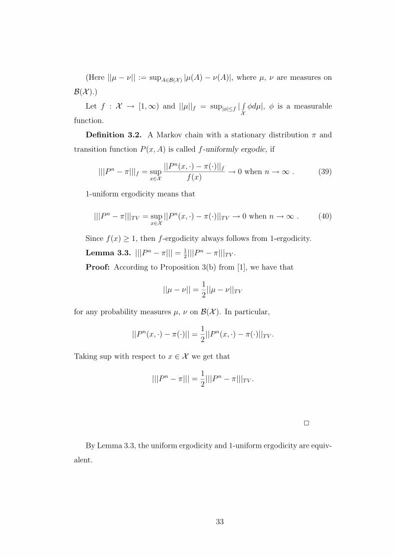
(Here ||µ − ν|| := supA∈B(X ) |µ(A) − ν(A)|, where µ, ν are measures on
B(X ).)
Let f : X → [1,∞) and ||µ||f = sup|φ|≤f |∫X
φdµ|, φ is a measurable
function.
Definition 3.2. A Markov chain with a stationary distribution π and
transition function P (x, A) is called f -uniformly ergodic, if
|||P n − π|||f = supx∈X
||P n(x, ·)− π(·)||ff(x)
→ 0 when n →∞ . (39)
1-uniform ergodicity means that
|||P n − π|||TV = supx∈X
||P n(x, ·)− π(·)||TV → 0 when n →∞ . (40)
Since f(x) ≥ 1, then f -ergodicity always follows from 1-ergodicity.
Lemma 3.3. |||P n − π||| = 12|||P n − π|||TV .
Proof: According to Proposition 3(b) from [1], we have that
||µ− ν|| = 1
2||µ− ν||TV
for any probability measures µ, ν on B(X ). In particular,
||P n(x, ·)− π(·)|| = 1
2||P n(x, ·)− π(·)||TV .
Taking sup with respect to x ∈ X we get that
|||P n − π||| = 1
2|||P n − π|||TV .
2
By Lemma 3.3, the uniform ergodicity and 1-uniform ergodicity are equiv-
alent.
33

3.1 Sufficient Conditions of f-Uniform Ergodicity for
Homogeneous Markov Chains
First, let’s state and proof a theorem which is sort of a corollary of what we
proved before.
Theorem 3.1.1. Let the conditions of Theorem 2.3.2 be satisfied and let
π be a stationary distribution for a given Markov chain. Then this Markov
chain is f -uniformly ergodic.
Proof: Without lost of generality we can assume that
γ = sup(x,x′)∈X×X
V (x, x′) < ∞
(see, for example, [1]). Therefore (ξ⊗ π)(V ) ≤ γ(ξ⊗ π)(X ×X ) = γ for any
ξ ∈ M(B(X )).
Fix δ > 0 and choose j = j(δ) so that
2(1− ε)j(b(1− λ)−1 + λn(ξ ⊗ π)(V )
)Ij≤n <
δ
2
for all n ≥ j.
Now let’s choose n(δ) > j(δ) so that
2λnBj(δ)−1(ξ ⊗ π)(V ) <δ
2
for n ≥ n(δ). Then, by Theorem 2.3.2, we have that
||ξP n − π||f < δ
for n ≥ n(δ) for all ξ ∈ M(B(X )).
Fix x ∈ X and take δ-measure
δx(A) =
1 if x ∈ A
0 if x /∈ A
Then we have
(δxPn)(φ) =
∫
Xφ(y)
∫
XP n(z, dy)δx(dz)
=(since
∫X
g(z)δx(dz) = g(x))
=∫
Xφ(y)P n(x, dy).
34

Therefore ||P n(x, ·)− π(·)||f = ||δxPn − π||f < δ for n ≥ n(δ) and for all
x ∈ X . Since f(x) ≥ 1, x ∈ X , then
|||P n − π||| = supx∈X
||P n(x.·)− π(·)||ff(x)
< δ
for n ≥ n(δ). This means that (39) holds, and, thus, chain X is f -uniformly
ergodic.
2
Now, let us give one more simple sufficient condition for f -uniform er-
godicity of Markov chain X = Xn∞n=0 with the state space (X ,B(X )) and
defined by a transition function P (x,A) and initial distribution µ. For this
purpose we shall need to recall the following definition of (n0, ε, ν)-small set:
Definition 3.1.2. A subset C ⊆ X is (n0, ε, ν)-small if there exist a
positive integer n0, ε > 0, and a probability measure ν on X such that the
following minorisation condition holds:
P n0(x,A) ≥ εν(A) (41)
for all x ∈ C, A ∈ B(X ).
Denote by M(B(X )) the set of all probability measures on B(X ).
Proposition 3.1.3. A subset C ⊂ X is (n0, ε, ν)-small if and only if
(ξP n0)(A) ≥ εν(A) (42)
for all ξ ∈ M(B(X )), A ∈ B(X ).
Proof: If (41) holds, ξ ∈ M(B(X )), then
(ξP n0)(A) =∫
XP n0(x, A)ξ(dx) ≥ εν(A)
∫
Xξ(dx) = εν(A),
i.e. (42) is true for all A ∈ B(X ).
35
Conversely, let (42) be true for all ξ ∈ M(B(X )), A ∈ B(X ). Fix x ∈ Xand take δ-measure δx(A). Then we have
εν(A) ≤ (δxPn0)(A) =
∫
XP n0(y,A)δx(dy) = P n0(x,A),
i.e. inequality (41) holds for all x ∈ X , A ∈ B(X ).
2
In the article [1] the following theorem is proved using the coupling
method:
Theorem 3.1.4. Let X be a (n0, ε, ν)-small set for a homogeneous
Markov chain X that has a stationary distribution π. Then ||P n(x, ·) −π(·)|| ≤ (1 − ε)[n/n0] for all x ∈ X , where [r] is the greatest integer not
exceeding r.
Since ||ξ|| = 12||ξ||TV for any ξ ∈ M(B(X )) (see Proposition 3 (b) in [1]),
then in terms of Theorem 3.1.4 we have that
||P n(x.·)− π(·)||TV ≤ 2(1− ε)[n/n0]
for all x ∈ X , and, thus,
supx∈X
||P n(x, ·)− π(·)||TV ≤ 2(1− ε)[n/n0].
This means that the Markov chain X is 1-uniformly ergodic.
Now let us give another proof of Theorem 3.1.4 without using the coupling
method. For this purpose we shall need the following
Proposition 3.1.5. Let X be a (n0, ε, ν)-small set. Then
||ξP n − ξ′P n||TV ≤ 2(1− ε)[n/n0] (43)
for all ξ, ξ′ ∈ M(B(X )).
Proof: By Proposition 3.1.3.,
ξ1(A) =(ξP n0)(A)− εν(A)
1− ε≥ 0;
36

ξ′1(A) =(ξ′P n0)(A)− εν(A)
1− ε≥ 0
for all A ∈ B(X ), and ξ1(X ) = 1 = ξ′(X ), i.e. ξ1, ξ′1 ∈ M(B(X )). Again
using condition (42), define
ξ2 =ξ1P
n0 − εν
1− ε∈ M(B(X ));
ξ′2 =ξ′1P
n0 − εν
1− ε∈ M(B(X )),
and
ξP n0 − ξ′P n0 = (1− ε)(ξ1 − ξ′1);
ξ1Pn0 − ξ′1P
n0 = (1− ε)(ξ2 − ξ′2),
and, thus,
ξP 2n0 − ξ′P 2n0 = (ξP n0 − ξ′P n0)P n0 = (1− ε)(ξ1Pn0 − ξ′1P
n0) = (1− ε)2(ξ2 − ξ′2).
Repeating this process, after k steps we’ll get that
ξP kn0 − ξ′P kn0 = (1− ε)k(ξk − ξ′k).
Any natural number n can be written as n = k + r, where k = [n/n0],
0 ≤ r < n0. Therefore
ξP n − ξ′P n = (ξP kn0 − ξ′P kn0)P r = (1− ε)k(ξk − ξ′k)Pr.
Let φ : X → [−1, 1] be a measurable function on (X ,B(X )). Then
|(ξP n)(φ)− (ξ′P n)(φ)| = (1− ε)k|(ξkPr)(φ)− (ξ′kP
r)(φ)|≤ (1− ε)k
((ξkP
r)(|φ|) + (ξ′kPr)(|φ|)
)
≤ (since |φ| ≤ 1) ≤≤ (1− ε)k
((ξkP
r)(1) + (ξ′kPr)(1)
)= 2(1− ε)k.
Thus,
||ξP n − ξ′P n||TV = sup|φ|≤1
|(ξP n)(φ)− (ξ′P n)(φ)| ≤ 2(1− ε)[n/n0]
37

for any ξ, ξ′ ∈ M(B(X )).
2
The proof of Theorem 3.1.4 is following from the equalities ||ξ|| = 12||ξ||TV ,
||P n(x, ·) − π(·)||TV = ||δxPn − π||TV (see the proof of theorem 3.1.1) and
inequality (43) for ξ′ = π.
Important Note: In terms of Theorem 3.1.3 we may not demand the
existence of a stationary distribution π, since its existence follows from the
condition that X is a (n0, ε, ν)-small set and the following proposition takes
place:
Proposition 3.1.6. Let X be a (n0, ε, ν)-small set for a homogeneous
Markov chain X. Then there exists a unique stationary distribution π for X.
Proof: Let ξ ∈ M(B(X )), m > n ≥ 1, k = m − n. Clear that ξP k =
ξ′ ∈ M(B(X )). From (43) it follows that
|(ξP n)(A)− (ξPm)(A)| = |(ξP n)(A)− (ξ′P n)(A)| ≤ 2(1− ε)[n/n0],
and,thus, (ξP n)(A) is a Cauchy sequence in R for all A ∈ B(X ). Therefore,
there exists a limit
πξ(A) = limn→∞(ξP n)(A).
By the well-known Vitali-Hahn-Saks Theorem (for references see [8], Chapter
IV, §2), πξ is a probability measure on B(X ), i.e. πξ ∈ M(B(X )), and
∫
Xφ(x)πξ(dx) = lim
n→∞
∫
Xφ(x)(ξP n)(dx)
for any bounded measurable function φ : X → R. In particular,
(πξ · P )(A) =∫
XP (x,A)πξ(dx) = lim
n→∞
∫
XP (x,A)(ξP n)(dx)
= limn→∞
∫
XP (x,A)
∫
XP n(y, dx)ξ(dy)
= limn→∞
∫
X
( ∫
XP (x,A)P n(y, dx)
)ξ(dy)
38

= limn→∞
∫
XP n+1(y,A)ξ(dy) = lim
n→∞(ξP n+1)(A)
= limn→∞(ξP n)(A) = πξ(A),
i.e. πξ · P = πξ, which means that πξ is a stationary distribution.
Similarly, for η ∈ M(B(X )) there exists a probability measure πη ∈M(B(X )) for which πη(A) = limn→∞(ηP n)(A) for all A ∈ B(X ). From
the inequality (43) it follows that
|(ξP n)(A)− (ηP n)(A)| → 0 when n →∞ ,
for all A ∈ B(X ). Therefore πξ = πη := π. In particular, if ηP = η, then
π(A) = (πη)(A) = limn→∞(ηP n)(A) = limn→∞ η(A) = η(A), A ∈ B(X ).
Thus, π is a unique stationary distribution for a Markov chain X.
2
From Propositions 3.1.4 and 3.1.6 we get the stronger version of Theorem
3.1.3:
Theorem 3.1.7. Let X be a (n0, ε, ν)-small set for a homogeneous
Markov chain X. Then X has a unique stationary distribution π and
||P n(x, ·)− π(·)|| ≤ (1− ε)[n/n0]
for all x ∈ X , in particular, X is 1-uniformly ergodic.
3.2 Necessary Conditions of f-Uniform Ergodicity for
Homogeneous Markov Chains
As shown in subsection 3.1, conditions (A1) and (A2) provide the f -uniform
ergodicity for homogeneous Markov chain. In the current subsection we shall
consider some versions of conditions (A1) and (A2) and show that they are
necessary conditions for f -uniform ergodicity of a Markov chain.
39

Recall that chain X is called φ-irreducible if there exists a non-zero σ-
finite measure φ on B(X ) such that for all A ∈ B(X ) with φ(A) > 0 and for
all x ∈ X there exists a positive integer n = n(x,A) such that P n(x,A) > 0.
The following proposition is obvious:
Proposition 3.2.1. Let X be a homogeneous Markov chain with a sta-
tionary distribution π and transition function P (x,A), which is f -uniformly
ergodic. Then X is π-irreducible.
The proof follows from (39).
The φ-irreducible Markov chains have many useful properties. One of
them is the existence of (n0, ε, ν)-small sets. The detailed proof of this fact
is given in [2] (theorems 5.2.1 and 5.2.2). Therefore we shall just state this
fact as a theorem:
Theorem 3.2.2. If X is φ-irreducible, then for every A ∈ B(X ) with
φ(A) > 0, there exists n0 ≥ 1, ε ∈ (0, 1) and (n0, ε, ν)-small set C ⊆ A such
that φ(C) > 0 and ν(C) > 0.
From Theorem 3.2.2 and Proposition 3.2.1 we get
Corollary 3.2.3. If a Markov chain X with a stationary distribution π
is f -uniformly ergodic, then there exists (n0, ε, ν)-small set C ∈ B(X ) for X
such that π(C) > 0.
We shall need the following simple criterion for f -uniform ergodicity of
Markov chains (see theorem 16.0.1 in [2]):
Proposition 3.2.4. For a Markov chain X with a stationary distribution
π and transition function P (x,A) the following conditions are equivalent:
(i) X is f -uniformly ergodic;
(ii) There exists r > 1 and L < ∞ such that for all n ∈ Z+
|||P n − π|||f ≤ Lr−n (44)
(iii) There exists some n ≥ 1 such that |||P i − π|||f < ∞ for i ≤ n and
|||P n − π|||f < 1. (45)
Proof: Implications (i) ⇒ (iii), (ii) ⇒ (i) and (ii) ⇒ (iii) are obvious.
40

Show (iii) ⇒ (ii). Let (iii) be satisfied. Since
(π · π)(A) =∫
Xπ(x,A)π(dx)
= (where π(x,A) = π(x) for all x ∈ X ) =
= π(A)∫
Xπ(dx) = π(A),
then from equalities
πP = π and (Pπ)(A) =∫
XP (x, dy)π(y, A) = π(A)
∫
XP (x, dy) = π(A)P (x,X ) = π(A)
we get that
(P n+1 − π)(A) = (P n − π)(P − π)(A).
Since for a measurable function ψ : (X ,B(X )) → R with |ψ| ≤ f we have
that
1
f|P n+1ψ − πψ| =
∣∣∣∣(P n − π)(P − π)(ψ)
f
∣∣∣∣
≤ |||P − π|||f · |(P n − π)(1)| (since |(P−π)(ψ)|f
≤ |||P − π|||f )
≤ |||P − π|||f ·∣∣∣∣(P n − π)(f)
f
∣∣∣∣
≤ |||P − π|||f · |||P n − π|||f .
Therefore,
|||P n+1 − π|||f ≤ |||P − π|||f · |||P n − π|||f .
Similarly, (P n+2 − π)(A) = (P n − π)(P 2 − π)(A), and therefore
|||P n+2 − π|||f ≤ |||P 2 − π|||f · |||P n − π|||f .
Continuing this process we’ll get that for any m ∈ Z+ the following
inequality is true: |||P n+m− π|||f ≤ |||Pm− π|||f · |||P n− π|||f . According to
(45), we have that γ = |||P n0−π|||f < 1 for some n0 ≥ 1 and |||P i−π||| < ∞,
i ≤ n0.
Any natural number n can be written in the form n = kn0 + i, where
k = [n/n0], 1 ≤ i < n0. Therefore
|||P n − π|||f = |||P kn0+i − π|||f ≤ |||P iπ|||f · |||P n0 − π|||kf ≤ Kγk,
41

where K = max1≤i<n0 |||P i − π|||f . Let L = K ·max1≤i<n0 γ− i
n0 , r = γ− 1
n0 .
Then
|||P n − π|||f ≤ Kγn−in0 = Kγ
− in0 · (γ 1
n0 )n ≤ Lr−n,
i.e. (44) is satisfied.
2
Definition 3.2.5. (See [2], §15.2.2) We say that chain X satisfies condi-
tion (f4), if there exist a real-valued function f : X → [1,∞), a set C ∈ B(X )
and constants λ ∈ (0, 1), b ∈ (0,∞) such that
Pf ≤ λf + bIC . (46)
Theorem 3.2.6. If the condition (f4) is satisfied for (n0, ε, ν)-small set
C, then the chain X is f -uniformly ergodic.
Proof: Consider a chain Y corresponding to the transition function
P n0(x,A), x ∈ X , A ∈ B(X ). Since C is (n0, ε, ν)-small for X, then C
is (1, ε, ν)-small for Y and, thus, for Y the condition (A1) is satisfied for
C = C × C.
Now, from (46) it follows that
P n0f = P n0−1(Pf) ≤ P n0−1(λf + bIC) ≤ λP n0−1f + b
≤ λ(λP n0−2f + b) + b ≤ ... ≤ λn0f + bn0−1∑
k=0
λk
≤ λn0f +b
1− λ(47)
Let β = 12(1 − λn0), D = x ∈ C : f(x) ≤ b
(1−λ)β. If x /∈ D, then
βf(x) > b1−λ
, and using (47), we have that
P n0f − f ≤ λn0f +b
1− λ− f = −2βf +
b
1− λ
= −βf + (b
1− λ− βf) ≤ −βf +
b
1− λID.
Thus,
P n0f ≤ (1− β)f +b
1− λID,
42
i.e. for the chain Y the condition (f4) is satisfied for the (1, ε, ν)-small set
D ⊂ C.
Take D = D×D. We shall get that for the chain Y the conditions (A1)
and (A2) are satisfied, and but Theorem 3.1.1, Y is f -uniformly ergodic, i.e.
(see Proposition 3.2.4)
|||Pmn0 − π|||f ≤ Lr−m
for some L > 0, r > 1 and all m = 1, 2, ....
Any n ≥ 1 can be written as n = kn0 + i, where k = [n/n0], 1 ≤ i < n0.
Then (see the proof of Proposition 3.2.2) we have
|||P n − π|||f ≤ |||P i − π|||f · |||P kn0 − π|||f ≤ K · Lr−k,
where K = max1≤i<n0 |||P i − π|||f . This means that |||P n − π|||f → 0 when
n →∞, i.e. the chain X is f -uniformly ergodic.
2
The next theorem shows that satisfaction of the condition (f4) for some
(n0, ε, ν)-small set is also a necessary condition for f -uniform ergodicity of
the chain (but instead of f we consider an equivalent to f function).
Theorem 3.2.7. If a chain X is f -uniformly ergodic, then X satisfies
the condition (f04) for some (n0, ε, ν)-small set, where 1kf ≤ f0 ≤ k for some
k ≥ 1.
Proof: According to Corollary 3.2.3, there exists a (n0, ε, ν)-small set C
for X. From Proposition 3.2.4 we have that
supx∈X
||P n − π||ff(x)
= |||P n − π|||f ≤ Lr−n
for some L > 0, r > 1 and all n = 1, 2, 3, .... Hence,
|P nf − π(f)| ≤ ||P n − π||f ≤ Lr−nf(x)
43

for all x ∈ X . Therefore,
P nf ≤ Lr−nf(x) + π(f) (48)
for all x ∈ X .
Fix n for which Lr−n < e−1 and set
f0(x) =n−1∑
i=0
ei/nP if ≥ e0P 0f = f(x).
From (48) it follows that
f0 ≤n−1∑
i=0
ein
(Lr−if + π(f)
)≤
( n−1∑
i=0
ein
)Lf + nπ(f)
≤ neLf + nπ(f) ≤ (since f(x) ≥ 1) ≤(neL + nπ(f)
)f ≤ kf
for big enough k > 1. Thus,
1
kf ≤ f ≤ f0 ≤ kf.
Now, using (48), we get
Pf0 = Pn−1∑
i=0
ein P if =
n∑
i=1
e( in− 1
n)P if
= e−1n
n−1∑
i=1
e1n P if + e1− 1
n P nf
≤ (since Lr−n < e−1) ≤ e−1n
n−1∑
i=1
ein P if + e−
1n f + e1− 1
n π(f)
= e−1n f0 + e1− 1
n π(f) = λ0f0 + b,
where λ0 = e−1n ∈ (0, 1), 0 ≤ b = e1− 1
n π(f) < ∞.
Repeating the part of the proof of Theorem 3.2.6 (the one after inequality
(47)), we get that
Pf0 ≤ (1− β)f0 +b
1− λID
for some (n0, ε, ν)-small set D ⊂ C, and this finishes the proof of the theorem.
2
44
From theorems 3.2.6 and 3.2.7 we obtain the following main theorem:
Theorem 3.2.8. Let X be a homogeneous Markov chain with a station-
ary distribution π, and let f : X → [1,∞). Then the following conditions
are equivalent:
(i) X is f -uniformly ergodic;
(ii) X satisfies condition (f04) for some (n0, ε, ν)-small set C and f0, where
1kf ≤ f0 ≤ kf for some k ≥ 1.
The End !!!
45

4 Appendix: The Topological Structure of
the State Space for Time-Homogeneous Markov
Chains
Let X be the state set for a time-homogeneous Markov chain defined by
the initial distribution π on a σ-algebra B of all subsets from X and the
transition function P (x,B), x ∈ X , B ∈ B. We require (X ,B) to be a
countably generated state space , i.e. there exists a countable subset D ⊂ Bfor which σ(D) = B, where σ(D) is the smallest σ-algebra of subsets from Xcontaining D (i.e. a σ-algebra generated by D).
It is known that σ-algebra B forms an algebraic ring, if we define the
algebraic operations on B as follows:
A + B := A4B = (A \B) ∪ (B \ A)
A ·B := A ∩B,
and then X \ A = X + A, A + A = ∅, A · A = A, X · A = A. Clear that
any subring A with identity X in (B, +, ·) is a subalgebra in B, since X ∈ A,
∅ = X + X ∈ A, X \ A = X + A ∈ A, ∀A ∈ A, and A ∩ B = A · B ∈ A∀A,B ∈ A.
Let’s take a subring D′ generated by a countable subset D and X , i.e.
D′ = ∑
i1,...,ik
Ai1 · · · Aik : Aij ∈ D, or Aij = X.
Clear that D′ is also countable.
Thus, we have the following
Proposition 4.1. If B is countably generated, then there exists a count-
able subalgebra D′ such that σ(D′) = B.
Now, let’s consider some probability measure P on B. Factor B with
respect to sets of measure zero, i.e. define an equivalence relationship on Bas follows:
A ∼ B if P (A4B) = 0.
46

Denote by ∇ = B|∼ the set of all equivalence classes. Define on ∇ the partial
order relationship: [A] ≤ [B], if ∃A′ ∈ [A], B′ ∈ [B] such that A′ ⊂ B′,
where [A] = D ∈ B : A ∼ D is an equivalence class containing set A.
With respect to this partial order (∇,≤) becomes a Boolean algebra. Recall:
Definition 4.2. A partially ordered set (∇,≤) is called a Boolean algebra,
if
1. (∇,≤) is a distributive lattice , i.e. ∀x, y ∈ ∇ there exist upper and
low bounds x ∨ y = sup(x, y), x ∧ y = inf(x, y), and
(x ∨ y) ∧ z = (x ∧ z) ∨ (y ∧ z) for all x, y, z ∈ ∇;
2. There exists the biggest element 1 ∈ ∇ (i.e. 1 ≥ x ∀x ∈ ∇) and the
smallest element 0 ∈ ∇ (i.e. 0 ≤ x ∀x ∈ ∇), such that 0 6= 1;
3. For all x ∈ ∇ there exists a complement xC ∈ ∇, i.e. an element such
that x ∨ xC = 1 and x ∧ xC = 0.
As an example of a Boolean algebra we can consider B for which the
partial order A ≤ B is defined as A ⊂ B. In this case, 1 = X , 0 = ∅,A ∨B = A ∪B, A ∧B = A ∩B, AC = X \ A.
So, we have a Boolean algebra ∇ = B|∼ and there is a measure µ on this
Boolean algebra defined by µ([A]) = P (A) (easy to check that if A ∼ A′,
then P (A) = P (A′), i.e. measure µ([A]) is well-defined).
Recall that a measure on a Boolean algebra∇ is a function ν : ∇ → [0,∞]
such that ν(e ∨ g) = ν(e) + ν(g), if e, g ∈ ∇, e ∧ g = 0. The measure ν is
called countably additive if
ν
( ∞∨
i=1
ei
)=
∞∑
i=1
ν(ei),
where ei ∈ ∇, ei ∧ ej = 0 for i 6= j. The measure ν is called strictly positive,
if from ν(e) = 0 it follows that e = 0.
We can state as a fact that the constructed measure µ([A]) = P (A) on
∇ = B|∼ is a strictly positive countably additive measure.
47

Definition 4.3. A Boolean algebra ∇ is called complete (σ-complete)
if for any collection eii∈I ⊂ ∇ (for any countable collection ei∞i=1 ⊂ ∇,
respectively) there exists
supi
ei =∨
i
ei ∈ ∇.
Definition 4.4. A Boolean algebra ∇ is of the countable type, if any
collection of non-zero pairwise disjoint elements from ∇ is countable (note:
by pairwise disjoint elements e, g ∈ ∇ we mean here that e ∧ g = 0).
The following proposition we state as a fact (for references see [6])
Proposition 4.5. (i) (see [6], chapter I, §6) If there exists a strictly
positive measure on ∇, then ∇ is of the countable type;
(ii) (see [6], chapter III, §2) If ∇ is a σ-complete Boolean algebra of the
countable type, then ∇ is a complete Boolean algebra.
Let ν be a strictly positive and countably additive measure on a σ-
complete algebra ∇ (in our case, ∇ = B|∼ is σ-complete, since B is a σ-
algebra and∨∞
i=1[Ai] =[ ⋃∞
i=1 Ai
], and µ is a strictly positive countably
additive measure on B|∼).
Consider a metrics ρ(e, g) on ∇ such that ρ(e, g) = ν(e + g). It’s known
Theorem 4.6. (see [6], chapter V, §1) (i) (∇, ρ) is a complete metric
space;
(ii) If ∇1 is a Boolean subalgebra in ∇, then the smallest σ-algebra in ∇containing ∇1 coincides with the closure ∇1 in (∇, ρ).
From Theorem 4.6 (ii) it follows that if there is a countable subalgebra
∇1 in ∇ such that ∇1 = ∇, then (∇, ρ) is a separable metric space. Thus,
we have
Corollary 4.7. (B|∼, ρ) is a complete separable metric space, where
ρ([A], [B]) = P (A4B).
Definition 4.8. An non-zero element q ∈ ∇ is called an atom in a
Boolean algebra ∇, if from q ≥ e 6= 0, e ∈ ∇ it follows that q = e. A Boolean
algebra is called atomic, if 1 = sup∆, where ∆ is the set of all atoms in
48
∇. A Boolean algebra which does not contain atoms is called a non-atomic
Boolean algebra.
Examples:
1. Let ∇ be a Boolean algebra of all subsets in X . Then every point
x = e is an atom in ∇, and 1 = X =⋃
x∈Xx, i.e. ∇ is an atomic
Boolean algebra.
2. The Boolean algebra B|∼, where B is a Lebesgue algebra on [0, 1] and
P is a Lebesgue measure, is a non-atomic Lebesgue algebra.
Theorem 4.9. (see [6], chapter III, §7) Let ∇ be a complete Boolean
algebra. Then there exists a unique element e0 ∈ ∇ such that e0 · ∇ = e ∈∇ : e ≤ e0 is a non-atomic Boolean algebra, eC
0 · ∇ = e ∈ ∇ : e ≤ eC0 is
an atomic Boolean algebra.
Now let’s discuss the structure of complete separable non-atomic and
atomic Boolean algebras.
Theorem 4.10. (see [7], chapter VIII, §41) Let (∇, ν) be a complete
separable non-atomic Boolean algebra. Then ∇ is isomorphic to a Boolean
algebra B|∼, where B is a σ-algebra of Lebesgue subsets on [0, 1], P is a
linear Lebesgue measure on [0, 1]. (Recall that two Boolean algebras ∇1
and ∇2 are isomorphic, if there exists a bijection φ : ∇1 → ∇2 such that
φ(e ∨ g) = φ(e) ∨ φ(g), φ(eC) = φ(e)C , in particular, φ(1) = 1, φ(0) = 0,
φ(e ∧ g) = φ(e) ∧ φ(g).)
It’s also known that
Proposition 4.11. If ∇ is a complete atomic Boolean algebra and ∆
is the set of all atoms in ∇, then ∇ is isomorphic to a Boolean algebra of
all subsets in ∆. In particular, if ∇ is separable, then ∆ is no more than
countable, and ∇ is a Boolean algebra of all subsets in a finite or countable
set.
From theorem 4.9 it follows that if ∇ is a complete Boolean algebra,
∇1 = e0∇ is a non-atomic Boolean algebra, ∇2 = eC0 ∇ is an atomic Boolean
49

algebra, then setting φ : ∇ → ∇1 × ∇2 defined by φ(e) = (e0e, eC0 e), we
get that φ is an isomorphism of Boolean algebras (note that ∇1 × ∇2 =
(e1, e2) : e1 ∈ ∇1, e2 ∈ ∇2 is a Boolean algebra with respect to the partial
order (e1, e2) ≤ (e′1, e′2) ⇔ e1 ≤ e′1, e2 ≤ e′2, and 1∇1×∇2 = (1∇1 ,1∇2),
0∇1×∇2 = (0∇1 ,0∇2), (e1, e2)∨ (g1, g2) = (e1∨ e2, g1∨ g2), (e1, e2)∧ (g1, g2) =
(e1 ∧ g1, e2 ∧ g2), (e1, e2)C = (eC
1 , eC2 )).
Thus, any complete Boolean algebra can be considered as collections of
elements (e, g), where e is from a non-atomic Boolean algebra, and g is from
an atomic Boolean algebra (with coordinate-wise Boolean operations).
Therefore, by theorem 4.10 and proposition 4.11, any complete separable
Boolean algebra can be interpreted as a Boolean algebra of collections of
elements (e, g), where e ∈ B[0, 1] - Lebesgue Boolean algebra on the interval
[0, 1], and g ∈ B(K) - σ-algebra of all subsets of a finite or countable set K.
Consider now Ω1 = [0, 1], F - Borel σ-algebra on [0, 1], P1 - linear
Lebesgue measure on F . If we extend P1 by Lebesgue, we get a Lebesgue
σ-algebra B1 and a complete Lebesgue measure P 1, extension of P1.
Let Ω2 = 1, ..., α, where α = n, or α = ∞, and B2 be a σ-algebra of all
subsets in Ω2. Let P2 be a probability measure on B2.
Let Ω = Ω1⋃
Ω2, A = A1 ∪ A2, A1 ∈ B1, A2 ∈ B2, P (A1 ∪ A2) =
P1(A1) + P2(A2). Consider ∇Ω = A|∼.
From above we have the following theorem (the main theorem in this
section):
Theorem 4.12. Let X be a set with a countably generated σ-algebra
B, and P be a probability on B. Then a Boolean algebra B|∼ is isomorphic
to ∇Ω.
Many examples of sets with countably generated σ-algebras are given by
complete separable metric spaces.
Let (X , ρ) be a complete separable metric space, B be a σ-algebra of
all its Borel subsets, i.e. the smallest σ-algebra containing all open subsets
from X . Since X is separable, X has a countable collection of open sets
50

such that all open sets can be obtained from their union. It means that
there exists a countable collection that generates B. If there is a probability
measure defined on B, then the Boolean algebra B|∼ is isomorphic to ∇Ω
(see theorem 4.12).
Conclusion: Talking about a general state set X for a homogeneous
Markov chain with an initial countably generated σ-algebra B, and keeping
in mind that P (x, ·) is a probability measure on B with respect to which
the Boolean algebra B|∼ has the same structure as ∇Ω, or, equivalently, as
a Boolean algebra of classes of equivalent Borel subsets of a complete sepa-
rable metric space, we can from the beginning assume that X is a complete
separable metric space, and B is a σ-algebra of Borel subsets in X .
The second argument to accept this conclusion is that for the study of
homogeneous Markov chains, defined by π and P (x,B), the central role is
played by probabilities and expectations on (X∞,⊗∞
i=1 B), defined as in (2)
and (3). Such construction is possible only with the help of Kolmogorov’s
theorem, which is true only for the case when X is a complete separable
metric space and B is a σ-algebra of Borel subsets in X .
Examples of Complete Separable Metric Spaces:
1. R;
2. Rn;
3. C[a, b] with ρ(f, g) = supt∈[a,b] |f(t)− g(t)|;
4. Any finite or countable set with a discrete metrics;
5. Any closed subset in a complete separable metric space is again a com-
plete separable metric set, i.e., for example, closed balls, parallelepipeds
in Rn are all complete separable.
51

References
[1] G.O. Roberts and J.S. Rosenthal, General state space Markov chains and
MCMC algorithms. Probability Surveys, 2004, 1, 20-71.
[2] S.P. Meyn and R.L. Tweedie. Markov Chains and Stochastic Stability.
1994, Springer-Verlag.
[3] R. Douc, E. Moulines, and J.S. Rosenthal, Quantitative bounds on con-
vergence of time-inhomogeneous Markov Chains. Annals of Applied Prob-
ability, 2004, 14, 1643–1665.
[4] Sh. A. Ayupov, T.A. Sarymsakov. About Homogeneous Markov Chains
on Semifields. Theory of Probability and Its Applications, 1981, v. XXVI,
3, 521-531 (Russian).
[5] A.N. Shiryaev. Probability. 1995, Springer-Verlag.
[6] D.A. Vladimirov. Boolean Algebras. 1969, Moscow, “Science” (Russian).
[7] P. Halmos. Measure Theory. 1950, New York.
[8] J. Neveu. Bases Mathematiques du Calcul des Probabilites. 1964, Paris.
Masson Et Cie.
52
Related Documents