ExtremeWeather: A large-scale climate dataset for semi ... · Of particular relevance is the TECA (Toolkit for Extreme Climate Analysis) Prabhat et al. (2012, 2015), an application

ExtremeWeather: A large-scale climate dataset forsemi-supervised detection, localization, andunderstanding of extreme weather events

Evan Racah1,2, Christopher Beckham1,3, Tegan Maharaj1,3,Samira Ebrahimi Kahou4, Prabhat2, Christopher Pal1,3

1 MILA, Université de Montréal, [email protected] Lawrence Berkeley National Lab, Berkeley, CA, [email protected].

3 École Polytechnique de Montréal, [email protected] Microsoft Maluuba, [email protected].

Abstract

Then detection and identification of extreme weather events in large-scale climatesimulations is an important problem for risk management, informing governmentalpolicy decisions and advancing our basic understanding of the climate system.Recent work has shown that fully supervised convolutional neural networks (CNNs)can yield acceptable accuracy for classifying well-known types of extreme weatherevents when large amounts of labeled data are available. However, many differenttypes of spatially localized climate patterns are of interest including hurricanes,extra-tropical cyclones, weather fronts, and blocking events among others. Existinglabeled data for these patterns can be incomplete in various ways, such as coveringonly certain years or geographic areas and having false negatives. This type ofclimate data therefore poses a number of interesting machine learning challenges.We present a multichannel spatiotemporal CNN architecture for semi-supervisedbounding box prediction and exploratory data analysis. We demonstrate that ourapproach is able to leverage temporal information and unlabeled data to improvethe localization of extreme weather events. Further, we explore the representationslearned by our model in order to better understand this important data. We presenta dataset, ExtremeWeather, to encourage machine learning research in this area andto help facilitate further work in understanding and mitigating the effects of climatechange. The dataset is available at extremeweatherdataset.github.io andthe code is available at https://github.com/eracah/hur-detect.

1 Introduction

Climate change is one of the most important challenges facing humanity in the 21st century, andclimate simulations are one of the only viable mechanisms for understanding the future impact ofvarious carbon emission scenarios and intervention strategies. Large climate simulations producemassive datasets: a simulation of 27 years from a 25 square km, 3 hour resolution model produces onthe order of 10TB of multi-variate data. This scale of data makes post-processing and quantitativeassessment challenging, and as a result, climate analysts and policy makers typically take globaland annual averages of temperature or sea-level rise. While these coarse measurements are usefulfor public and media consumption, they ignore spatially (and temporally) resolved extreme weatherevents such as extra-tropical cyclones and tropical cyclones (hurricanes). Because the general publicand policy makers are concerned about the local impacts of climate change, it is critical that we beable to examine how localized weather patterns (such as tropical cyclones), which can have dramaticimpacts on populations and economies, will change in frequency and intensity under global warming.

31st Conference on Neural Information Processing Systems (NIPS 2017), Long Beach, CA, USA.

Deep neural networks, especially deep convolutional neural networks, have enjoyed breakthrough suc-cess in recent recent years, achieving state-of-the-art results on many benchmark datasets (Krizhevskyet al., 2012; He et al., 2015; Szegedy et al., 2015) and also compelling results on many practicaltasks such as disease diagnosis (Hosseini-Asl et al., 2016), facial recognition (Parkhi et al., 2015),autonomous driving (Chen et al., 2015), and many others. Furthermore, deep neural networkshave also been very effective in the context of unsupervised and semi-supervised learning; somerecent examples include variational autoencoders (Kingma & Welling, 2013), adversarial networks(Goodfellow et al., 2014; Makhzani et al., 2015; Salimans et al., 2016; Springenberg, 2015), laddernetworks (Rasmus et al., 2015) and stacked what-where autoencoders (Zhao et al., 2015).

There is a recent trend towards video datasets aimed at better understanding spatiotemporal relationsand multimodal inputs (Kay et al., 2017; Gu et al., 2017; Goyal et al., 2017). The task of findingextreme weather events in climate data is similar to the task of detecting objects and activities invideo - a popular application for deep learning techniques. An important difference is that in the caseof climate data, the ’video’ has 16 or more ’channels’ of information (such as water vapour, pressureand temperature), while conventional video only has 3 (RGB). In addition, climate simulations do notshare the same statistics as natural images. As a result, unlike many popular techniques for video, wehypothesize that we cannot build off successes from the computer vision community such as usingpretrained weights from CNNs (Simonyan & Zisserman, 2014; Krizhevsky et al., 2012) pretrained onImageNet (Russakovsky et al., 2015).

Climate data thus poses a number of interesting machine learning problems: multi-class classificationwith unbalanced classes; partial annotation; anomaly detection; distributional shift and bias correction;spatial, temporal, and spatiotemporal relationships at widely varying scales; relationships betweenvariables that are not fully understood; issues of data and computational efficiency; opportunitiesfor semi-supervised and generative models; and more. Here, we address multi-class detection andlocalization of four extreme weather phenomena: tropical cyclones, extra-tropical cyclones, tropicaldepressions, and atmospheric rivers. We implement a 3D (height, width, time) convolutional encoder-decoder, with a novel single-pass bounding-box regression loss applied at the bottleneck. To ourknowledge, this is the first use of a deep autoencoding architecture for bounding-box regression. Thisarchitectural choice allows us to do semi-supervised learning in a very natural way (simply trainingthe autoencoder with reconstruction for unlabelled data), while providing relatively interpretablefeatures at the bottleneck. This is appealing for use in the climate community, as current engineeredheuristics do not perform as well as human experts for identifying extreme weather events.

Our main contributions are (1) a baseline bounding-box loss formulation; (2) our architecture, a firststep away from engineered heuristics for extreme weather events, towards semi-supervised learnedfeatures; (3) the ExtremeWeather dataset, which we make available in three benchmarking splits: onesmall, for model exploration, one medium, and one comprising the full 27 years of climate simulationoutput.

2 Related work

2.1 Deep learning for climate and weather data

Climate scientists do use basic machine learning techniques, for example PCA analysis for dimen-sionality reduction (Monahan et al., 2009), and k-means analysis for clusterings Steinhaeuser et al.(2011). However, the climate science community primarily relies on expert engineered systems andad-hoc rules for characterizing climate and weather patterns. Of particular relevance is the TECA(Toolkit for Extreme Climate Analysis) Prabhat et al. (2012, 2015), an application of large scalepattern detection on climate data using heuristic methods. A more detailed explanation of how TECAworks is described in section 3. Using the output of TECA analysis (centers of storms and boundingboxes around these centers) as ground truth, (Liu et al., 2016) demonstrated for the first time thatconvolutional architectures could be successfully applied to predict the class label for two extremeweather event types. Their work considered the binary classification task on centered, cropped patchesfrom 2D (single-timestep) multi-channel images. Like (Liu et al., 2016) we use TECA’s output(centers and bounding boxes) as ground truth, but we build on the work of Liu et al. (2016) by: 1)using uncropped images, 2) considering the temporal axis of the data 3) doing multi-class boundingbox detection and 4) taking a semi-supervised approach with a hybrid predictive and reconstructivemodel.

2

Some recent work has applied deep learning methods to weather forecasting. Xingjian et al. (2015)have explored a convolutional LSTM architecture (described in 2.2 for predicting future precipitationon a local scale (i.e. the size of a city) using radar echo data. In contrast, we focus on extremeevent detection on planetary-scale data. Our aim is to capture patterns which are very local in time(e.g. a hurricane may be present in half a dozen sequential frames), compared to the scale of ourunderlying climate data, consisting of global simulations over many years. As such, 3D CNNsseemed to make more sense for our detection application, compared to LSTMs whose strength is incapturing long-term dependencies.

2.2 Related methods and modelsFollowing the dramatic success of CNNs in static 2D images, a wide variety of CNN architectureshave been explored for video, ex. (Karpathy et al., 2014; Yao et al., 2015; Tran et al., 2014). Thedetails of how CNNs are extended to capture the temporal dimension are important. Karpathy et al.(2014) explore different strategies for fusing information from 2D CNN subcomponents; in contrast,Yao et al. (2015) create 3D volumes of statistics from low level image features.

Convolutional networks have also been combined with RNNs (recurrent neural networks) for mod-eling video and other sequence data, and we briefly review some relevant video models here. Themost common and straightforward approach to modeling sequential images is to feed single-framerepresentations from a CNN at each timestep to an RNN. This approach has been examined fora number of different types of video (Donahue et al., 2015; Ebrahimi Kahou et al., 2015), while(Srivastava et al., 2015) have explored an LSTM architecture for the unsupervised learning of videorepresentations using a pretrained CNN representation as input. These architectures separate learningof spatial and temporal features, something which is not desirable for climate patterns. Anotherpopular model, also used on 1D data, is a convolutional RNN, wherein the hidden-to-hidden transitionlayer is 1D convolutional (i.e. the state is convolved over time). (Ballas et al., 2016) combine theseideas, applying a convolutional RNN to frames processed by a (2D) CNN.

The 3D CNNs we use here are based on 3-dimensional convolutional filters, taking the height, width,and time axes into account for each feature map, as opposed to aggregated 2D CNNs. This approachwas studied in detail in (Tran et al., 2014). 3D convolutional neural networks have been used forvarious tasks ranging from human activity recognition (Ji et al., 2013), to large-scale YouTube videoclassification (Karpathy et al., 2014), and video description (Yao et al., 2015). Hosseini-Asl et al.(2016) use a 3D convolutional autoencoder for diagnosing Alzheimer’s disease through MRI - intheir case, the 3 dimensions are height, width, and depth. (Whitney et al., 2016) use 3D (height,width, depth) filters to predict consecutive frames of a video game for continuation learning. Recentwork has also examined ways to use CNNs to generate animated textures and sounds (Xie et al.,2016). This work is similar to our approach in using 3D convolutional encoder, but where theirapproach is stochastic and used for generation, ours is deterministic, used for multi-class detectionand localization, and also comprises a 3D convolutional decoder for unsupervised learning.

Stepping back, our approach is related conceptually to (Misra et al., 2015), who use semi-supervisedlearning for bounding-box detection, but their approach uses iterative heuristics with a support vectormachine (SVM) classifer, an approach which would not allow learning of spatiotemporal features.Our setup is also similar to recent work from (Zhang et al., 2016) (and others) in using a hybridprediction and autoencoder loss. This strategy has not, to our knowledge, been applied either tomultidimensional data or bounding-box prediction, as we do here. Our bounding-box prediction lossis inspired by (Redmon et al., 2015), an approach extended in (Ren et al., 2015), as well as the singleshot multiBox detector formulation used in (Liu et al., 2015) and the seminal bounding-box work inOverFeat (Sermanet et al., 2013). Details of this loss are described in Section 4.

3 The ExtremeWeather dataset3.1 The Data

The climate science community uses three flavors of global datasets: observational products (satellite,gridded weather station); reanalysis products (obtained by assimilating disparate observationalproducts into a climate model) and simulation products. In this study, we analyze output from thethird category because we are interested in climate change projection studies. We would like to betterunderstand how Earth’s climate will change by the year 2100; and it is only possible to conduct

3

such an analysis on simulation output. Although this dataset contains the past, the performance ofdeep learning methods on this dataset can still inform the effectiveness of these approaches on futuresimulations. We consider the CAM5 (Community Atmospheric Model v5) simulation, which is astandardized three-dimensional, physical model of the atmosphere used by the climate community tosimulate the global climate (Conley et al., 2012). When it is configured at 25-km spatial resolution(Wehner et al., 2015), each snapshot of the global atmospheric state in the CAM5 model output is a768x1152 image, having 16 ’channels’, each corresponding to a different simulated variable (likesurface temperature, surface pressure, precipitation, zonal wind, meridional wind, humidity, cloudfraction, water vapor, etc.). The global climate is simulated at a temporal resolution of 3 hours, giving8 snapshots (images) per day. The data we provide is from a simulation of 27 years from 1979 to2005. In total, this gives 78,840 16-channel 768x1152 images.

3.2 The Labels

Ground-truth labels are created for four extreme weather events: Tropical Depressions (TD) TropicalCyclones (TC), Extra-Tropical Cyclones (ETC) and Atmospheric Rivers (AR) using TECA (Prabhatet al., 2012). TECA generally works by suggesting candidate coordinates for storm centers byonly selecting points that follow a certain combination of criteria, which usually involves requiringvarious variables’ (such as pressure, temperature and wind speed) values are between between certainthresholds. These candidates are then refined by breaking ties and matching the "same" storms acrosstime (Prabhat et al., 2012). These storm centers are then used as the center coordinates for boundingboxes. The size of the boxes is determined using prior domain knowledge as to how big these stormsusually are, as described in (Liu et al., 2016). Every other image (i.e. 4 per day) is labeled due tocertain design decisions made during the production run of the TECA code. This gives us 39,420labeled images.

3.2.1 Issues with the Labels

TECA, the ground truth labeling framework, implements heuristics to assign ’ground truth’ labelsfor the four types of extreme weather events. However, it is entirely possible there are errors in thelabeling: for instance, there is little agreement in the climate community on a standard heuristic forcapturing Extra-Tropical Cyclones (Neu et al., 2013); Atmospheric Rivers have been extensivelystudied in the northern hemisphere (Lavers et al., 2012; Dettinger et al., 2011), but not in the southernhemisphere; and spatial extents of such events not universally agreed upon. In addition, this labelingonly includes AR’s in the US and not in Europe. As such, there is potential for many false negatives,resulting in partially annotated images. Lastly, it is worth mentioning that because the ground truthgeneration is a simple automated method, a deep, supervised method can only do as well as emulatingthis class of simple functions. This, in addition to lower representation for some classes (AR andTD), is part of our motivation in exploring semi-supervised methods to better understand the featuresunderlying extreme weather events rather than trying to "beat" existing techniques.

3.3 Suggested Train/Test Splits

We provide suggested train/test splits for the varying sizes of datasets on which we run experiments.Table 1 shows the years used for train and test for each dataset size. We show "small" (2 yearstrain, 1 year of test), "medium" (8 years train, 2 years test) and "large" (22 years train, 5 yearstest) datasets. For reference, table 2 shows the breakdown of the dataset splits for each class for"small" in order to illustrate the class-imbalance present in the dataset. Our model was trained on"small", where we split the train set 50:50 for train and validation. Links for downloading trainand test data, as well as further information the different dataset sizes and splits can be found here:extremeweatherdataset.github.io.

Table 1: Three benchmarking levels for the ExtremeWeather dataset

Level Train Test

Small 1979, 1981 1984Medium 1979-1983,1989-1991 1984-1985Large 1979-1983, 1994-2005, 1989-1993 1984-1988

4

Table 2: Number of examples in ExtremeWeather benchmark splits, with class breakdown statisticsfor Tropical Cyclones (TC), Extra-Tropical Cyclones (ETC), Tropical Depressions (TD), and UnitedStates Atmospheric Rivers (US-AR)

Benchmark Split TC (%) ETC (%) TD (%) US-AR (%) TotalSmall Train 3190 (42.32) 3510 (46.57) 433 (5.74) 404 (5.36) 7537

Test 2882 (39.04) 3430 (46.47) 697 (9.44) 372 (5.04) 7381

4 The modelWe use a 3D convolutional encoder-decoder architecture, meaning that the filters of the convolutionalencoder and decoder are 3 dimensional (height, width, time). The architecture is shown in Figure 1;the encoder uses convolution at each layer while the decoder is the equivalent structure in reverse,using tied weights and deconvolutional layers, with leaky ReLUs (Andrew L. Maas & Ng., 2013)(0.1) after each layer. As we take a semi-supervised approach, the code (bottleneck) layer of theautoencoder is used as the input to the loss layers, which make predictions for (1) bounding boxlocation and size, (2) class associated with the bounding box, and (3) the confidence (sometimescalled ’objectness’) of the bounding box. Further details (filter size, stride length, padding, outputsizes, etc.) can be found in the supplementary materials.

Figure 1: Diagram of the 3D semi-supervised architecture. Parentheses denote subset of totaldimension shown (for ease of visualization, only two feature maps per layer are shown for theencoder-decoder. All feature maps are shown for bounding-box regression layers).

The total loss for the network, L, is a weighted combination of supervised bounding-box regressionloss, Lsup, and unsupervised reconstruction error, Lrec :

L = Lsup + λLrec, (1)

where Lrec is the mean squared squared difference between input X and reconstruction X∗:

Lrec =1

M||X −X∗||22, (2)

where M is the total number of pixels in an image.

In order to regress bounding boxes, we split the original 768x1152 image into a 12x18 grid of64x64 anchor boxes. We then predict a box at each grid point by transforming the representation to12x18=216 scores (one per anchor box). Each score encodes three pieces of information: (1) howmuch the predicted box differs in size and location from the anchor box, (2) the confidence that anobject of interest is in the predicted box (“objectness”), and (3) the class probability distribution forthat object. Each component of the score is computed by several 3x3 convolutions applied to the 64012x18 feature maps of the last encoder layer. Because each set of pixels in each feature map at agiven x, y coordinate can be thought of as a learned representation of the climate data in a 64x64patch of the input image, we can think of the 3x3 convolutions as having a local receptive field size of192x192, so they use a representation of a 192x192 neighborhood from the input image as context todetermine the box and object centered in the given 64x64 patch. Our approach is similar to (Liu et al.,2015) and (Sermanet et al., 2013), which use convolutions from small local receptive field filters to

5

regress boxes. This choice is motivated by the fact that extreme weather events occur in relativelysmall spatiotemporal volumes, with the ‘background’ context being highly consistent across eventtypes and between events and non-events. This is in contrast to Redmon et al. (2015), which usesa fully connected layer to consider the whole image as context, appropriate for the task of objectidentification in natural images, where there is often a strong relationship between background andobject.

The bounding box regression loss, Lsup, is determined as follows:

Lsup =1

N(Lbox + Lconf + Lcls), (3)

where N is the number of time steps in the minibatch, and Lbox is defined as:

Lbox = α∑i

1obji R(ui − u∗i ) + β

∑i

1obji R(vi − v∗i ), (4)

where i ∈ [0, 216) is the index of the anchor box for the ith grid point, and where 1obji = 1 if an

object is present at the ith grid point, 0 if not; R(z) is the smooth L1 loss as used in (Ren et al., 2015),ui = (tx, ty)i and u∗i = (t∗x, t

∗y)i, vi = (tw, th)i and v∗i = (t∗w, t

∗h)i and t is the parametrization

defined in (Ren et al., 2015) such that:

tx = (x− xa)/wa, ty = (y − ya)/ha, tw = log(w/wa), th = log(h/ha)

t∗x = (x∗ − xa)/wa, t∗y = (y∗ − ya)/ha, t∗w = log(w∗/wa), t

∗h = log(h∗/ha),

where (xa, ya, wa, ha) is the center coordinates and height and width of the closest anchor box,(x, y, w, h) are the predicted coordinates and (x∗, y∗, w∗, h∗) are the ground truth coordinates.

Lconf is the weighted cross-entropy of the log-probability of an object being present in a grid cell:

Lconf =∑i

1obji [− log(p(obj)i)] + γ ∗

∑i

1noobji [− log(p(obji))] (5)

Finally Lcls is the cross-entropy between the one-hot encoded class distribution and the softmaxpredicted class distribution, evaluated only for predicted boxes at the grid points containing a groundtruth box:

Lcls =∑i

1obji

∑c∈classes

−p∗(c) log(p(c)) (6)

The formulation of Lsup is similar in spirit to YOLO (Redmon et al., 2015), with a few importantdifferences. Firstly, the object confidence and class probability terms in YOLO are squared-differencesbetween ground truth and prediction, while we use cross-entropy, as used in the region proposalnetwork from Faster R-CNN (Ren et al., 2015) and the network from (Liu et al., 2015), for theobject probability term and the class probability term respectively. Secondly, we use a differentparametrization for the coordinates and the size of the bounding box. In YOLO, the parametrizationsfor x and y are equivalent to Faster R-CNN’s tx and ty , for an anchor box the same size as the patchit represents (64x64). However w and h in YOLO are equivalent to Faster-RCNN’s th and tw for a64x64 anchor box only if (a) the anchor box had a height and width equal to the size of the wholeimage and (b) there were no log transform in the faster-RCNN’s parametrization. We find boththese differences to be important in practice. Without the log term, and using ReLU nonlinearitiesinitialized (as is standard) centered around 0, most outputs (more than half) will give initial boxesthat are in 0 height and width. This makes learning very slow, as the network must learn to resizeessentially empty boxes. Adding the log term alone in effect makes the "default" box (an outputof 0) equal to the height and width of the entire image - this equally slows down learning, becausethe network must now learn to drastically shrink boxes. Making ha and wa equal to 64x64 is apragmatic ’Goldilocks’ value. This makes training much more efficient, as optimization can focusmore on picking which box contains an object and not as much on what size the box should be.Finally, where YOLO uses squared difference between predicted and ground truth for the coordinateparametrizations, we use smooth L1, due its lower sensitivity to outlier predictions (Ren et al., 2015).

6

5 Experiments and Discussion

5.1 Framewise Reconstruction

As a simple experiment, we first train a 2D convolutional autoencoder on the data, treating eachtimestep as an individual training example (everything else about the model is as described in Section4), in order to visually assess reconstructions and ensure reasonable accuracy of detection. Figure2 shows the original and reconstructed feature maps for the 16 climate variables of one image inthe training set. Reconstruction loss on the validation set was similar to the training set. As thereconstruction visualizations suggest, the convolutional autoencoder architecture does a good job ofencoding spatial information from climate images.

original reconstruction

Figure 2: Feature maps for the 16 channels in an ’image’ from the training set (left) and theirreconstructions from the 2D convolutional autoencoder (right).

5.2 Detection and localization

All experiments are on ExtremeWeather-small, as described in Section 3, where 1979 is train and1981 is validation. The model is trained with Adam (Kingma & Ba, 2014), with a learning rate of0.0001 and weight decay coefficient of 0.0005. For comparison, and to evaluate how useful the timeaxis is to recognizing extreme weather events, we run experiments with both 2D (width, height)and 3D (width, height, time) versions of the architecture described in Section 4. Values for α, β, γ(hyperparameters described in loss Equations 4 and 5) were selected with experimentation and someinspiration from (Redmon et al., 2015) to be 5, 7 and 0.5 respectively. A lower value for γ pushes upthe confidence of true positive examples, allowing the model more examples to learn from, is thus away to deal with ground-truth false negatives. Although some of the selection of these parameters isa bit ad-hoc, we assert that our results still provide a good first-pass baseline approach for this dataset.The code is available at https://github.com/eracah/hur-detect

During training, we input one day’s simulation at a time (8 time steps; 16 variables). The semi-supervised experiments reconstruct all 8 time steps, predicting bounding boxes for the 4 labelledtimesteps, while the supervised experiments reconstruct and predict bounding boxes only for the4 labelled timesteps. Table 3 shows Mean Average Precision (mAP) for each experiment. AveragePrecision (AP) is calculated for each class in the manner of ImageNet (Russakovsky et al., 2015),integrating the precision-recall curve, and mAP is averaged over classes. Results are shown forvarious settings of λ (see Equation 1) and for two modes of evaluation; at IOU (intersection over unionof the bounding-box and ground-truth box) thresholds of 0.1 and 0.5. Because the 3D model hasinherently higher capacity (in terms of number of parameters) than the 2D model, we also experimentwith higher capacity 2D models by doubling the number of filters in each layer. Figure 3 showsbounding box predictions for 2 consecutive (6 hours in between) simulation frames, comparing the3D supervised vs 3D semi-supervised model predictions.

It is interesting to note that 3D models perform significantly better than their 2D counterparts forETC and TC (hurricane) classes. This implies that the time evolution of these weather events isan important criteria for discriminating them. In addition, the semi-supervised model significantlyimproves the ETC and TC performance, which suggests unsupervised shaping of the spatio-temporalrepresentation is important for these events. Similarly, semi-supervised data improves performanceof the 3D model (for IOU=0.1), while this effect is not observed for 2D models, suggesting that 3Drepresentations benefit more from unsupervised data. Note that hyperparameters were tuned in thesupervised setting, and a more thorough hyperparameter search for λ and other parameters may yieldbetter semi-supervised results.

7

Figure 3 shows qualitatively what the quantitative results in Table 3 confirm - semi-supervisedapproaches help with rough localization of weather events, but the model struggles to achieveaccurate boxes. As mentioned in Section 4, the network has a hard time adjusting the size of theboxes. As such, in this figure we see mostly boxes of size 64x64. For example, for TDs (usuallymuch smaller than 64x64) and for ARs, (always much bigger than 64x64), a 64x64 box roughlycentered on the event is sufficient to count as a true positive at IOU=0.1, but not at the more stringentIOU=0.5. This lead to a large dropoff in performance for ARs and TDs, and a sizable dropoff in the(variably-sized) TCs. Longer training time could potentially help address these issues.

Table 3: 2D and 3D supervised and semi-supervised results, showing Mean Average Precision (mAP)and Average Precision (AP) for each class, at IOU=0.1; IOU=0.5. M is model; P is millions ofparameters; and λ weights the amount that reconstruction contributes to the overall loss.

M Mode P λETC (46.47%)

AP (%)TC (39.04%)

AP (%)TD (9.44%)

AP (%)AR (5.04%)

AP (%) mAP2D Sup 66.53 0 21.92; 14.42 52.26; 9.23 95.91; 10.76 35.61; 33.51 51.42; 16.982D Semi 66.53 1 18.05; 5.00 52.37; 5.26 97.69; 14.60 36.33; 0.00 51.11; 6.212D Semi 66.53 10 15.57; 5.87 44.22; 2.53 98.99; 28.56 36.61; 0.00 48.85; 9.242D Sup 16.68 0 13.90; 5.25 49.74; 15.33 97.58; 7.56 35.63; 33.84 49.21; 15.492D Semi 16.68 1 15.80; 9.62 39.49; 4.84 99.50; 3.26 21.26; 13.12 44.01; 7.713D Sup 50.02 0 22.65; 15.53 50.01; 9.12 97.31; 3.81 34.05; 17.94 51.00; 11.603D Semi 50.02 1 24.74; 14.46 56.40; 9.00 96.57; 5.80 33.95; 0.00 52.92; 7.31

Figure 3: Bounding box predictions shown on 2 consecutive (6 hours in between) simulation frames,for the integrated water vapor column channel. Green = ground truth, Red = high confidencepredictions (confidence above 0.8). 3D supervised model (Left), and semi-supervised (Right).

5.3 Feature explorationIn order to explore learned representations, we use t-SNE (van der Maaten & Hinton, Nov 2008)to visualize the autoencoder bottleneck (last encoder layer). Figure 4 shows the projected featuremaps for the first 7 days in the training set for both 3D supervised (top) and semi-supervised (bottom)experiments. Comparing the two, it appears that more TCs (hurricanes) are clustered by the semi-supervised model, which would fit with the result that semi-supervised information is particularlyvaluable for this class. Viewing the feature maps, we can see that both models have learned spiralpatterns for TCs and ETCs.

6 Conclusions and Future WorkWe introduce to the community the ExtremeWeather dataset in hopes of encouraging new researchinto unique, difficult, and socially and scientifically important datasets. We also present a baselinemethod for comparison on this new dataset. The baseline explores semi-supervised methods for

8

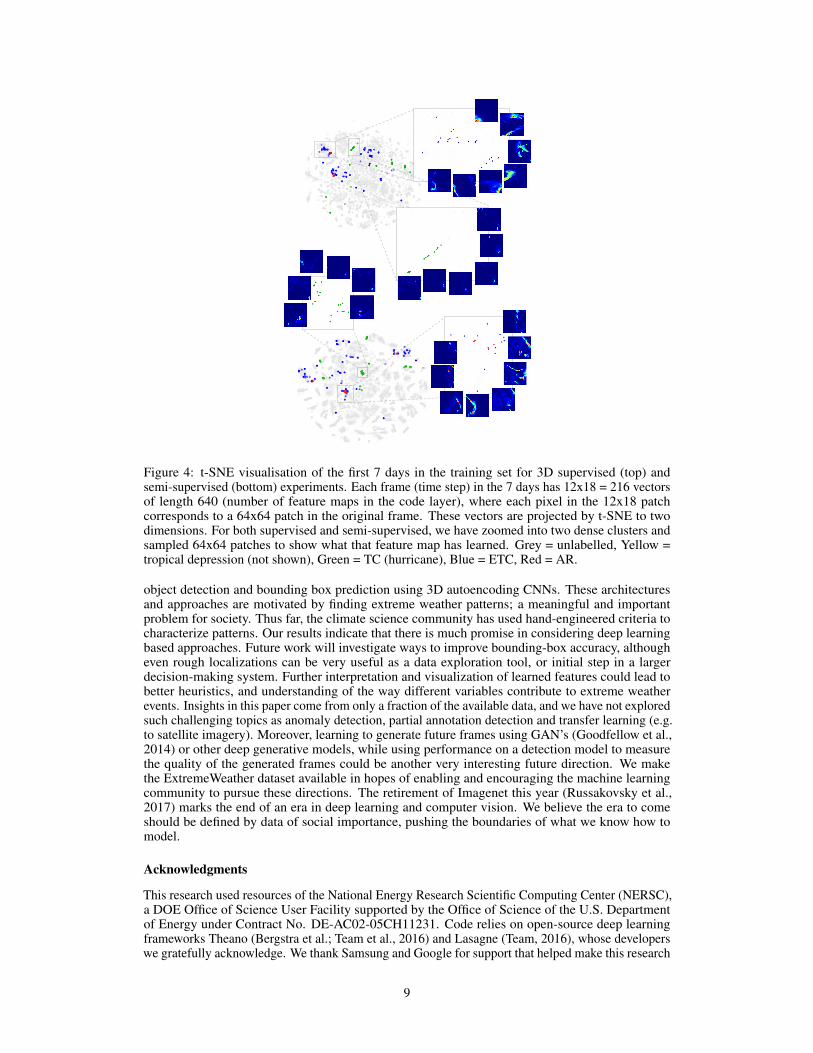
Figure 4: t-SNE visualisation of the first 7 days in the training set for 3D supervised (top) andsemi-supervised (bottom) experiments. Each frame (time step) in the 7 days has 12x18 = 216 vectorsof length 640 (number of feature maps in the code layer), where each pixel in the 12x18 patchcorresponds to a 64x64 patch in the original frame. These vectors are projected by t-SNE to twodimensions. For both supervised and semi-supervised, we have zoomed into two dense clusters andsampled 64x64 patches to show what that feature map has learned. Grey = unlabelled, Yellow =tropical depression (not shown), Green = TC (hurricane), Blue = ETC, Red = AR.

object detection and bounding box prediction using 3D autoencoding CNNs. These architecturesand approaches are motivated by finding extreme weather patterns; a meaningful and importantproblem for society. Thus far, the climate science community has used hand-engineered criteria tocharacterize patterns. Our results indicate that there is much promise in considering deep learningbased approaches. Future work will investigate ways to improve bounding-box accuracy, althougheven rough localizations can be very useful as a data exploration tool, or initial step in a largerdecision-making system. Further interpretation and visualization of learned features could lead tobetter heuristics, and understanding of the way different variables contribute to extreme weatherevents. Insights in this paper come from only a fraction of the available data, and we have not exploredsuch challenging topics as anomaly detection, partial annotation detection and transfer learning (e.g.to satellite imagery). Moreover, learning to generate future frames using GAN’s (Goodfellow et al.,2014) or other deep generative models, while using performance on a detection model to measurethe quality of the generated frames could be another very interesting future direction. We makethe ExtremeWeather dataset available in hopes of enabling and encouraging the machine learningcommunity to pursue these directions. The retirement of Imagenet this year (Russakovsky et al.,2017) marks the end of an era in deep learning and computer vision. We believe the era to comeshould be defined by data of social importance, pushing the boundaries of what we know how tomodel.

Acknowledgments

This research used resources of the National Energy Research Scientific Computing Center (NERSC),a DOE Office of Science User Facility supported by the Office of Science of the U.S. Departmentof Energy under Contract No. DE-AC02-05CH11231. Code relies on open-source deep learningframeworks Theano (Bergstra et al.; Team et al., 2016) and Lasagne (Team, 2016), whose developerswe gratefully acknowledge. We thank Samsung and Google for support that helped make this research

9

possible. We would also like to thank Yunjie Liu and Michael Wehner for providing access to theclimate datasets; Alex Lamb and Thorsten Kurth for helpful discussions.

ReferencesAwni Y. Hannun Andrew L. Maas and Andrew Y. Ng. Rectifier nonlinearities improve neural network

acoustic models. ICML Workshop on Deep Learning for Audio, Speech, and Language Processing,2013.

Nicolas Ballas, Li Yao, Chris Pal, and Aaron Courville. Delving deeper into convolutional networksfor learning video representations. In the Proceedings of ICLR. arXiv preprint arXiv:1511.06432,2016.

Chenyi Chen, Ari Seff, Alain Kornhauser, and Jianxiong Xiao. Deepdriving: Learning affordance fordirect perception in autonomous driving. In Proceedings of the IEEE International Conference onComputer Vision, pp. 2722–2730, 2015.

Andrew J Conley, Rolando Garcia, Doug Kinnison, Jean-Francois Lamarque, Dan Marsh, MikeMills, Anne K Smith, Simone Tilmes, Francis Vitt, Hugh Morrison, et al. Description of the ncarcommunity atmosphere model (cam 5.0). 2012.

Michael D. Dettinger, Fred Martin Ralph, Tapash Das, Paul J. Neiman, and Daniel R. Cayan.Atmospheric rivers, floods and the water resources of california. Water, 3(2):445, 2011. ISSN2073-4441. URL http://www.mdpi.com/2073-4441/3/2/445.

Jeffrey Donahue, Lisa Anne Hendricks, Sergio Guadarrama, Marcus Rohrbach, Subhashini Venu-gopalan, Kate Saenko, and Trevor Darrell. Long-term recurrent convolutional networks for visualrecognition and description. In The IEEE Conference on Computer Vision and Pattern Recognition(CVPR), June 2015.

Samira Ebrahimi Kahou, Vincent Michalski, Kishore Konda, Roland Memisevic, and ChristopherPal. Recurrent neural networks for emotion recognition in video. In Proceedings of the 2015 ACMon International Conference on Multimodal Interaction, pp. 467–474. ACM, 2015.

Ian Goodfellow, Jean Pouget-Abadie, Mehdi Mirza, Bing Xu, David Warde-Farley, Sherjil Ozair,Aaron Courville, and Yoshua Bengio. Generative adversarial nets. In Advances in NeuralInformation Processing Systems, pp. 2672–2680, 2014.

Raghav Goyal, Samira Kahou, Vincent Michalski, Joanna Materzynska, Susanne Westphal, HeunaKim, Valentin Haenel, Ingo Fruend, Peter Yianilos, Moritz Mueller-Freitag, et al. The "somethingsomething" video database for learning and evaluating visual common sense. arXiv preprintarXiv:1706.04261, 2017.

Chunhui Gu, Chen Sun, Sudheendra Vijayanarasimhan, Caroline Pantofaru, David A Ross, GeorgeToderici, Yeqing Li, Susanna Ricco, Rahul Sukthankar, Cordelia Schmid, et al. Ava: A videodataset of spatio-temporally localized atomic visual actions. arXiv preprint arXiv:1705.08421,2017.

Kaiming He, Xiangyu Zhang, Shaoqing Ren, and Jian Sun. Delving deep into rectifiers: Surpassinghuman-level performance on imagenet classification. In Proceedings of the IEEE InternationalConference on Computer Vision, pp. 1026–1034, 2015.

Ehsan Hosseini-Asl, Georgy Gimel’farb, and Ayman El-Baz. Alzheimer’s disease diagnostics by adeeply supervised adaptable 3d convolutional network. 2016.

Shuiwang Ji, Wei Xu, Ming Yang, and Kai Yu. 3d convolutional neural networks for human actionrecognition. IEEE transactions on pattern analysis and machine intelligence, 35(1):221–231,2013.

Andrej Karpathy, George Toderici, Sanketh Shetty, Thomas Leung, Rahul Sukthankar, and Li Fei-Fei.Large-scale video classification with convolutional neural networks. In Proceedings of the IEEEconference on Computer Vision and Pattern Recognition, pp. 1725–1732, 2014.

10

Will Kay, Joao Carreira, Karen Simonyan, Brian Zhang, Chloe Hillier, Sudheendra Vijayanarasimhan,Fabio Viola, Tim Green, Trevor Back, Paul Natsev, et al. The kinetics human action video dataset.arXiv preprint arXiv:1705.06950, 2017.

Diederik Kingma and Jimmy Ba. Adam: A method for stochastic optimization. arXiv preprintarXiv:1412.6980, 2014.

Diederik P Kingma and Max Welling. Auto-encoding variational bayes. arXiv preprintarXiv:1312.6114, 2013.

Alex Krizhevsky, Ilya Sutskever, and Geoffrey E Hinton. Imagenet classification with deep convolu-tional neural networks. In Advances in neural information processing systems, pp. 1097–1105,2012.

David A. Lavers, Gabriele Villarini, Richard P. Allan, Eric F. Wood, and Andrew J. Wade. Thedetection of atmospheric rivers in atmospheric reanalyses and their links to british winter floodsand the large-scale climatic circulation. Journal of Geophysical Research: Atmospheres, 117(D20):n/a–n/a, 2012. ISSN 2156-2202. doi: 10.1029/2012JD018027. URL http://dx.doi.org/10.1029/2012JD018027. D20106.

Wei Liu, Dragomir Anguelov, Dumitru Erhan, Christian Szegedy, and Scott Reed. Ssd: Single shotmultibox detector. arXiv preprint arXiv:1512.02325, 2015.

Yunjie Liu, Evan Racah, Prabhat, Joaquin Correa, Amir Khosrowshahi, David Lavers, KennethKunkel, Michael Wehner, and William Collins. Application of deep convolutional neural networksfor detecting extreme weather in climate datasets. 2016.

Alireza Makhzani, Jonathon Shlens, Navdeep Jaitly, and Ian J. Goodfellow. Adversarial autoencoders.CoRR, abs/1511.05644, 2015. URL http://arxiv.org/abs/1511.05644.

Ishan Misra, Abhinav Shrivastava, and Martial Hebert. Watch and learn: Semi-supervised learningof object detectors from videos. CoRR, abs/1505.05769, 2015. URL http://arxiv.org/abs/1505.05769.

Adam H Monahan, John C Fyfe, Maarten HP Ambaum, David B Stephenson, and Gerald R North.Empirical orthogonal functions: The medium is the message. Journal of Climate, 22(24):6501–6514, 2009.

Urs Neu, Mirseid G. Akperov, Nina Bellenbaum, Rasmus Benestad, Richard Blender, RodrigoCaballero, Angela Cocozza, Helen F. Dacre, Yang Feng, Klaus Fraedrich, Jens Grieger, SergeyGulev, John Hanley, Tim Hewson, Masaru Inatsu, Kevin Keay, Sarah F. Kew, Ina Kindem,Gregor C. Leckebusch, Margarida L. R. Liberato, Piero Lionello, Igor I. Mokhov, Joaquim G.Pinto, Christoph C. Raible, Marco Reale, Irina Rudeva, Mareike Schuster, Ian Simmonds, MarkSinclair, Michael Sprenger, Natalia D. Tilinina, Isabel F. Trigo, Sven Ulbrich, Uwe Ulbrich,Xiaolan L. Wang, and Heini Wernli. Imilast: A community effort to intercompare extratropicalcyclone detection and tracking algorithms. Bulletin of the American Meteorological Society, 94(4):529–547, 2013. doi: 10.1175/BAMS-D-11-00154.1.

Omkar M Parkhi, Andrea Vedaldi, and Andrew Zisserman. Deep face recognition. In British MachineVision Conference, volume 1, pp. 6, 2015.

Prabhat, Oliver Rubel, Surendra Byna, Kesheng Wu, Fuyu Li, Michael Wehner, and Wes Bethel.Teca: A parallel toolkit for extreme climate analysis. ICCS, 2012.

Prabhat, Surendra Byna, Venkatram Vishwanath, Eli Dart, Michael Wehner, and William D. Collins.Teca: Petascale pattern recognition for climate science. CAIP, 2015.

Antti Rasmus, Mathias Berglund, Mikko Honkala, Harri Valpola, and Tapani Raiko. Semi-supervisedlearning with ladder networks. In Advances in Neural Information Processing Systems, pp. 3546–3554, 2015.

Joseph Redmon, Santosh Kumar Divvala, Ross B. Girshick, and Ali Farhadi. You only look once:Unified, real-time object detection. CoRR, abs/1506.02640, 2015. URL http://arxiv.org/abs/1506.02640.

11

Shaoqing Ren, Kaiming He, Ross Girshick, and Jian Sun. Faster r-cnn: Towards real-time objectdetection with region proposal networks. 2015.

Olga Russakovsky, Jia Deng, Hao Su, Jonathan Krause, Sanjeev Satheesh, Sean Ma, Zhiheng Huang,Andrej Karpathy, Aditya Khosla, Michael Bernstein, et al. Imagenet large scale visual recognitionchallenge. International Journal of Computer Vision, 115(3):211–252, 2015.

Olga Russakovsky, Eunbyung Park, Wei Liu, Jia Deng, Fei-Fei Li, and Alex Berg. Beyond imagenetlarge scale visual recognition challenge, 2017. URL http://image-net.org/challenges/beyond_ilsvrc.php.

Tim Salimans, Ian Goodfellow, Wojciech Zaremba, Vicki Cheung, Alec Radford, and Xi Chen.Improved techniques for training gans. 2016.

Pierre Sermanet, David Eigen, Xiang Zhang, Michaël Mathieu, Rob Fergus, and Yann LeCun.Overfeat: Integrated recognition, localization and detection using convolutional networks. arXivpreprint arXiv:1312.6229, 2013.

Karen Simonyan and Andrew Zisserman. Very deep convolutional networks for large-scale imagerecognition. arXiv preprint arXiv:1409.1556, 2014.

Jost Tobias Springenberg. Unsupervised and semi-supervised learning with categorical generativeadversarial networks. arXiv preprint arXiv:1511.06390, 2015.

Nitish Srivastava, Elman Mansimov, and Ruslan Salakhutdinov. Unsupervised learning of videorepresentations using lstms. CoRR, abs/1502.04681, 2, 2015.

Karsten Steinhaeuser, Nitesh Chawla, and Auroop Ganguly. Comparing predictive power in climatedata: Clustering matters. Advances in Spatial and Temporal Databases, pp. 39–55, 2011.

Christian Szegedy, Wei Liu, Yangqing Jia, Pierre Sermanet, Scott Reed, Dragomir Anguelov, Du-mitru Erhan, Vincent Vanhoucke, and Andrew Rabinovich. Going deeper with convolutions. InProceedings of the IEEE Conference on Computer Vision and Pattern Recognition, pp. 1–9, 2015.

Du Tran, Lubomir Bourdev, Rob Fergus, Lorenzo Torresani, and Manohar Paluri. Learning spa-tiotemporal features with 3d convolutional networks. 2014.

L.J.P van der Maaten and G.E. Hinton. Visualizing high-dimensional data using t-sne. Journal ofMachine Learning Research, 9: 2579–2605, Nov 2008.

Michael Wehner, Prabhat, Kevin A. Reed, Dáithí Stone, William D. Collins, and Julio Bacmeister.Resolution dependence of future tropical cyclone projections of cam5.1 in the u.s. clivar hurricaneworking group idealized configurations. Journal of Climate, 28(10):3905–3925, 2015. doi:10.1175/JCLI-D-14-00311.1.

William F. Whitney, Michael Chang, Tejas Kulkarni, and Joshua B. Tenenbaum. Understandingvisual concepts with continuation learning. 2016.

Jianwen Xie, Song-Chun Zhu, and Ying Nian Wu. Synthesizing dynamic textures and sounds byspatial-temporal generative convnet. 2016.

Shi Xingjian, Zhourong Chen, Hao Wang, Dit-Yan Yeung, Wai-kin Wong, and Wang-chun Woo.Convolutional lstm network: A machine learning approach for precipitation nowcasting. InAdvances in Neural Information Processing Systems, pp. 802–810, 2015.

Li Yao, Atousa Torabi, Kyunghyun Cho, Nicolas Ballas, Christopher Pal, Hugo Larochelle, andAaron Courville. Describing videos by exploiting temporal structure. In Proceedings of the IEEEInternational Conference on Computer Vision, pp. 4507–4515, 2015.

Yuting Zhang, Kibok Lee, and Honglak Lee. Augmenting supervised neural networks with un-supervised objectives for large-scale image classification. arXiv preprint arXiv:1606.06582v1,2016.

Junbo Zhao, Michael Mathieu, Ross Goroshin, and Yann Lecun. Stacked what-where auto-encoders.arXiv preprint arXiv:1506.02351, 2015.

12