Extreme Coexceedances in New EU Member States’ Stock Markets

Extreme Coexceedances in New EU MemberStates’ Stock Markets∗

Charlotte Christiansen†

University of Aarhus & CREATESAngelo Ranaldo‡

Swiss National Bank

November 7, 2007

∗The views expressed herein are those of the authors and not necessarily those of theSwiss National Bank, which does not accept any responsibility for the contents and opinionsexpressed in this paper. Christiansen acknowledges support from CREATES funded by theDanish National Research Foundation. The authors gratefully acknowledge helpful commentsand suggestions from Susanne Bonomo, Michael Rockinger, and Sébastien Wälti, as well asfrom seminar participants at the CREATES Opening Conference, and at the SNB.

†School of Economics and Management, University of Aarhus, Building 1322, Uni-versitetsparken, 8000 Aarhus C, Denmark. Phone: +45 8942 5477. Email:[email protected].

‡Research Department, Swiss National Bank, Switzerland. Email:[email protected].

Extreme Coexceedances in New EU MemberStates’ Stock Markets

Abstract: We analyze the financial integration of the new EU member states’

stock markets using the coexceedance variable that counts the number of large

negative returns on a given day across the countries. We use a multinomial

logit model to investigate which factors influence the coexceedance variable;

separately for geographical effects, asset class effects, volatility effects, and per-

sistence effects. The effects differ for negative (large negative returns) and posi-

tive (large positive returns) coexceedance variables. The coexceedance variables

for the old and the new EU countries are influenced differently. The effects on

the new EU coexceedance variables change after the EU enlargement in 2004.

Keywords: Emerging markets; EU enlargement; EU Member States; Extreme

returns; Financial integration; New EU Member States; Stock Markets

JEL Classifications: C25; F36; G15

1 Introduction

How do extreme price jumps propagate across countries? How are the relations

of forces between developed and emerging markets in these circumstances? Do

price disruptions in one region lead or lag extreme price movements in anther

one? Do extreme price movements spill over across asset classes? In which

market conditions is it more likely to observe contagion? Does the prospect

of adopting a common currency have any bearing on the contagion phenom-

enon? This paper attempts to shed some light on these and related important

questions.

In times of financial crisis investors and policy makers have a very strong

interest in whether the crisis propagates to other countries; this is known as

contagion effects. The past has for instance seen the “Asian flu” that started in

Thailand in 1997 and propagated around the world. The way international mar-

kets reacted to recent events such as 9/11, the Second Gulf War, and hurricanes

Rita and Katrina suggests that contagion is increasingly a global phenomenon.

In this paper we investigate the interaction and contagion effects in the emerg-

ing and developed European stock markets. This provides valuable information

about the typical market conditions and dynamics leading to joint price falls

or rises in European countries. We analyze three main aspects of the conta-

gion phenomenon between established and emerging European stock markets:

geographical aspects, asset classes’ interdependence, and dominant market con-

ditions such as risk perception and propagation timing. These research questions

should highlight the anatomy of contagion, the transmission mechanism within

and between regions and any asymmetry between positive and negative spillover

effects.

The European Union (EU) enlargement in 2004 might be considered a nat-

ural experiment to observe the effects of the plan of adopting a common currency

on financial markets. For the new EU member states that are developing coun-

tries, this event represents a unique case to examine the effects of such policy

decision on emerging stock markets. However, one can argue that the enlarge-

ment mechanism is more about adopting the EU legislation rather than the

effects of a common currency and, in addition, that it is unfair to generalize

this issue since each country distinguishes itself by its own unique socioeco-

nomic characteristics. In his seminal work, Mundell (1961) pointed out the

main trade-off for adopting a common currency. On the one hand, a common

currency represents a reduction of transaction costs. On the other hand, it im-

plies the loss of the natural "shock absorbers" represented by flexible exchange

rates and independent monetary policies. The specific questions we address in

3

this study is whether and to what extent the contagion phenomenon within new

member states has changed after their adhesion to the EU.

In the literature, there is yet little convergence of definitions and terminol-

ogy. A number of authors call for discrimination between the terms "pure

contagion", "interdependence", "shock propagation", "transmission effects",

"spillovers" and so on (see, e.g., Forbes and Rigobon (2002)). Previously, con-

tagion was mainly measured by the correlation between the returns at differ-

ent financial markets. Among other disadvantages, correlation may be biased

by conditional heteroskedasticity (see Boyer, Gibson and Loretan (1999) and

Forbes and Rigobon (2002)).

Bae, Karolyi and Stulz (2003) suggest measuring contagion by how often

extreme returns on different markets occur simultaneous. Extreme returns are

large positive and large negative returns. Bae et al. (2003) count the number

of coexistence of extreme returns (positive and negative separately) in different

emerging stock markets in the same region. In this way, their definition of

contagion is implicitly alike to correlation but yet it overcomes the problems

mentioned above of the definition of contagion as well as the problems of using

correlation to measure contagion. They use the multinomial logit model to

explain the number of coexistence of extreme returns in Asia and Latin America.

They find that contagion depends on interest rates, exchange rate changes and

conditional stock return volatility. In this paper we apply a similar method to

investigate the factors that explain the comovement between the stock markets

in the new EU member states from the previous Communist states of Central

and Eastern Europe. The lessons from the euro adoption indicate that EU

membership might have strong implications for the integration of the individual

financial markets. Also, the new EU member states aim at adopting the euro,

and in fact some did so at the beginning of 2007, so they have strong interests

in their markets becoming more integrated with the markets of old European

member states and we pay special attention to effects stemming from their entry

to the EU.

Methodologically we mainly lean on Bae et al. (2003), however other papers

use related methods to investigate contagion effects. Cumperayot, Keijzer and

Kouwenberg (2006) use a bivariate probit model for the extreme currency event

and the extreme stock event as the explanatory variables. The model is esti-

mated separately for 26 countries. Extreme stock market events are found to

increase the likelihood of extreme currency events. Fazio (forthcoming) looks

at bivariate probit models for crisis variables for a pair of countries. Contagion

emerges if the error terms are correlated. The crisis variable is a measure of

4

speculative pressure depending on the exchange rate and level of international

reserves. Hartmann, Straetmans and de Vries (2004) use extreme value theory

to model the expected number of market crashes given that at least one market

has already crashed. Their empirical analysis covers the five largest industrial-

ized countries. Chan-Lau, Methieson and Yao (2004) also apply extreme value

theory to analyze contagion in Latin America and Asia.

In general, the new EU member states’ asset markets are becoming more

integrated with the old EU member states’ asset markets. Cappiello, Gérard,

Kadareja and Manganelli (2006) consider the integration of seven new EU coun-

tries’ stock markets using quantile regressions to make so-called comovement

plots. They find that the integration within the new EU countries and with

the old EU countries increases over time, and that it is mainly due to the three

largest markets, (the Czech Republic, Hungary, and Poland). Moore and Wang

(2007) consider the volatility of five new EU member states’ stock markets.

They show that the stock volatility decreases when the state enters the EU, i.e.

the stock markets tend to be in the low volatility states. They use a regime

switching model so that they do not have to use the exact entry date to in-

vestigate the effect of EU entry. Dovak and Podpiera (2006) investigate the

stock returns in the new EU member states after the announcement of the en-

largement of the EU. They use firm-specific data to calculate betas. They find

that part of the stock price increase is connected to differences between local

and world betas. Dovak (2007) shows that the new EU member states’ bond

yields (government and corporate) have moved towards the levels in the old EU

countries.

Using the coexceedance methodology of Bae et al. (2003) we investigate the

contagion between the stock markets in the 10 new EU member states from

the former Communist countries in Eastern and Central Europe. The negative

coexceedance variable for the new EU countries counts the number of extreme

returns (below 5 percentile) across the new EU countries on a given day. The

positive coexceedance variable for the new EU (above 95 percentile) and the

negative and positive coexceedance variables for the new EU are constructed

analogously. Using the multivariate logit model, we investigate which factors

influence the coexceedance variables. We distinguish between four hypotheses

that are investigated separately, namely geographical effects, asset class effects,

volatility effects, and persistence effects. The effects from the explanatory vari-

ables are of the expected signs. We find that negative coexceedances in the new

EU stock markets are significantly influenced by US stock return, old EU stock

return, new EU stock return, old EU stock volatility, interest rate volatility,

5

lagged negative coexceedance for new EU, and negative coexceedance for old

EU. Moreover we find that the factors that influence the coexceedance variables

differ for the old and new EU stock markets. More specifically, we find that

coexceedances among old EU states appear more connected to US stock mar-

kets and to extreme price movements into other asset classes. The coexceedance

factors also differ for the positive and negative coexceedance variables. In par-

ticular, negative coexceedances for new EU stock markets show up when turmoil

is a common factor across world regions and asset classes. Finally, we find that

the new EU markets appear more dependent on old EU countries after the EU

enlargement in May 2004.

The structure of the remaining part of the paper is as follows: In Section 2

we present the data and in Section 3 we explain the empirical set-up. Section 4

contains the empirical results and Section 5 concludes.

2 Data Description

Here we describe the data: first the coexceedance variables that we use as

explained variables in the regressions to come, and second, the explanatory

variables that enter those regressions.

We consider the following ten new EU member states: Bulgaria, the Czech

Republic, Estonia, Hungary, Latvia, Lithuania, Poland, Romania, Slovakia, and

Slovenia. Notice that we focus on the new EU member states from the former

Communist Central and Eastern European countries, i.e. we exclude two new

EU member states, Cyprus and Malta, which are small population-wise and

Mediterranean. Bulgaria and Romania joined the EU on January 1, 2007, the

other countries on May 1, 2004.1 We consider the joining countries as one group

irrespective of whether they joined the EU in 2004 or in 2007.

The group of old EU countries consists of Austria, Belgium, Denmark, Fin-

land, France, Germany, Greece, Ireland, Italy, the Netherlands, Portugal, Spain,

Sweden, and the UK.

We apply daily data for the stock markets for various European countries.

When available we use the DataStream stock index. In a few cases we instead

use the relevant index from the local stock market because the DataStream

index is not available. This applies to Estonia, Latvia, Lithuania, Slovakia, and

Slovenia.

We use daily log returns from the total return indexes for the stock markets

1We excluded Luxemburg for obvious reasons of data availability (e.g. no stock marketindex exists).

6

measured in local currency.2 The data cover the period from October 2, 2000 to

April 20, 2007 which gives us a total of 1710 observations. This can be viewed

as a representative sample period including both bull and bear phases, high and

low volatility environments and different market conditions.34

2.1 Coexceedance Variables

It is from the log returns that we define the extreme returns. We follow Bae

et al. (2003) and use the 5% and 95% percentiles to define the negative and

positive extreme returns, respectively.5 We treat large positive and negative

returns separately.

We treat the new and old EU member states separately. We construct a

variable that counts the number of extreme positive returns for the new EU

countries on a given day. The variable can take on integer values between 0

and 10. We collect observations of 4 and above into one group, so the variable

is truncated to take on values between 0 and 4. We denote this variable the

positive coexceedance variable for the new EU countries. A similar positive

coexceedance variable is constructed for the old EU countries. The negative

coexceedance variable for the new EU countries is constructed by counting the

number of negative extreme returns on the new EU stock markets on a given

day. Finally, we construct the negative coexceedance variable for the old EU

countries. We use the following notation for the coexceedance variables.

• XNnewt : negative coexceedance for new EU countries on day t

• XNoldt : negative coexceedance for old EU countries on day t

• XPnewt : positive coexceedance for new EU countries on day t

• XP oldt : positive coexceedance for old EU countries on day t

Summary statistics for the coexceedance variables are given in Table 1. Most

of the days, there are no instances of extreme returns. 64% and 76% of the days

there are no extreme negative returns in the new EU countries and the old

2Local currency returns are equivalent to currency hedged returns. Using common currencyreturns would bias the results and confound the genuine stock performance with that of theexchange rates.

3October 2, 2000 is the earliest date with daily stock market data for all the countriesunder investigation.

4We do the same analysis using a shorter sample period, namely beginning in August 2002.We performed this additional analysis in order to compare two well-defined bull periods, i.e.from August 2002 to April 2004 and after May 2004. This allows us to see whether the bullmarkets may bias our results. The results are very similar.

5The 5% and 95% percentiles are supposed to be the best compromise to capture thefarthest portions of the distribution tails and to get representative samples of extreme returns.

7

EU countries, respectively. The figures are slightly higher for extreme positive

returns (66% and 77%). For positive extreme returns, 11% of the days have

more than one new EU member states with a positive extreme return. This

applies to 12% of the old EU states. There are slightly more days with more

than one extreme negative return in the new EU countries (namely 12% of the

days). This also applies to the old EU countries where this happens 13% of the

days. IT is the days with more than one extreme return that we are trying to

explain by various factors in the empirical analysis to come.

Figure 1 shows the time series plot of the four coexceedance variables. We

see that the instances of several coexceedances are spread out during the sample

period and are not confined to a limited period of time.

2.2 Explanatory Variables

In the empirical analysis, in addition to the coexceedance variables we also make

use of the variables below that are used as explanatory variables in various logit

models. We have a sample of daily observations for which the sample period

matches that for the coexceedance variables.

• SUSt : Concurrent return from the US stock market (DataStream index)

• Soldt : Concurrent return for European stock market (DataStream index

for Western Europe)

• Snewt : Concurrent return for new EU stock market (log-returns from

equally weighted index constructed for the Czech Republic, Hungary, and

Poland)

• σoldt : Concurrent volatility for old European stock return (square root of

variance from AR(1)-GARCH(1,1) model for SUSt )

• Ct: Concurrent currency log return (exchange rate of GDM/euro per

USD)

• σCt : Concurrent volatility for currency return (square root of variance

from AR(1)-GARCH(1,1) model for Ct)

• Rt: Concurrent interest rate (first differences of 1-month EURIBOR (Euro

Interbank Offered Rate), first differences because unit root cannot be re-

jected)6

• σRt : Concurrent interest rate volatility (square root of variance from AR(1)-

GARCH(1,1) of first differences of Rt)6 It does not seem to be of importance whether we use a US or a European interest rate.

8

3 Empirical Set-Up

In first part of this section, we present the econometric technique. The second

part describes the hypotheses to test.

3.1 Multinomial Logit Model for Coexceedances

We conduct univariate analysis and model one coexceedance variable at the

time. The coexceedance variables are discrete choice variables, which can be

modelled using a multinomial discrete choice model, such as the logit model we

apply here. By considering only five categories (0, 1, 2, 3, and 4 and above) we

reduce the number of parameters and make the results easier to understand.

In the multinomial logit model the probability of (say) XNnewt being in

category i where i = 0, 1, 2, 3, 4 the distribution is given by

Pi =exp

³β0

ix´

1 +4X

j=1,j 6=iexp

³β0jx´

where x is the vector of explanatory variables (including a constant) and βi is

the vector of coefficients. There is one coefficient for each covariate for each of

the categories. In this way we can test whether the number of coexceedances is

explained significantly by a given variable. For simplicity below, we state that

the probability of being in category i is given as a function of the explanatory

variables: Pi = function(β0ix) where i = 1, 2, 3, 4.

We estimate the multinomial logit model using different sets of explanatory

variables, more hereon follows below.

We access the goodness of fit of the various models by using a χ2 test for

the significance of all the explanatory variables, i.e. where we compare the

estimated model with the base line model that only has the constant term as

explanatory variable. We also use the base line model to calculate a pseudo R2

which is not adjusted for the number of parameters. We use a χ2 test to access

the significance of a given explanatory variable, i.e. whether all the coefficients

to all the categories are insignificant simultaneously.

The multinomial logit model is estimated using PCGive in OxMetrics. Un-

less otherwise noted we apply a 5% level of significance.

9

3.2 Testable Hypotheses

We investigate four main hypotheses (H1-H4) that relate to which factors in-

fluence the likelihood of the coexceedance variables taking on large values, i.e.

showing contagion. The hypotheses relate to geographical effects, asset class

effects, volatility effects, and persistence effects. For each hypothesis we use

a separate logit model for the four coexceedance variables. By using separate

models for each of the four hypothesis we avoid any problems of multicolinearity.

Also, it makes the results easier to interpret. However, we might incur problems

of omitted variables. We find the latter argument to of less importance.7

The fifth hypothesis (H5) relates to asymmetry effects between positive and

negative extreme returns. In each case we also investigate whether the influence

of the variables upon the coexceedance variables for the new EU states change

when the first group of the former Eastern Block countries joined the EU in May

2004 (H6). The hypotheses that we investigate are described in detail below.

3.2.1 H1: Geographical Effects

In correspondence with the gravity law in physics, Rose (2000) proposes to

explain the flow of international trade between a pair of countries as being pro-

portional to their economic "mass" (read "income") and inversely proportional

to the distance between them. By analogy, the main reasons behind financial

crisis transmission from one country to another can be the size of the interna-

tional capital markets and their geographical location. Geographical proximity

and larger market capitalization should increase the likelihood of transmission.

From this perspective, one would expect that sharp market movements tend

to move from old to new EU member states because of the geographical close-

ness and economic partnership. However, the US equity market is the largest

market worldwide, one can also expect that contagion effects come from the

US market. It is worth asking whether these forces have changed after the EU

enlargement. One could expect that the link between new and old EU member

states has become stronger and that after the financial market integration of new

EU member states within the EU zone, new EU members are more responsive

to international shocks.7We performed several regressions accommodating all explanatory variables or different

combinations of them. This additional analysis essentially suggests that the bias of omittedvariables does not hold.

10

3.2.2 H2: Asset Class Effects

One important reason behind financial crisis transmission across asset classes is

an abrupt portfolio re-allocation in times of flight-to-quality (e.g. Caballero and

Krishnamurthy (2007)), and these effects can be reinforced by liquidity spirals

(Brunnermeier and Pedersen (2007)). These arguments suggest a substitution

effect between equities and safer assets such as bonds or money market instru-

ments. Extreme price interdependence between short-term bonds, equities and

currencies can arise at unanticipated news announcements and monetary policy

decisions. Other sources of transmission especially relevant for emerging mar-

kets are currency attacks (Morris and Shin (1998) and Obstfeld (1986)) and

unwinding carry trade (Bank for International Settlements (1999)). According

to these arguments, we expect that coexceedances in equity markets be con-

nected with large price movements in bond and currency markets.

Additionally, the EU membership may have (1) decreased the currency risk

premium and (2) increased the degree of equity return correlation within new

member states and between them and old member states. As pointed out by

Adjaouté and Danthine (2003), these effects may be intensified by a higher

integration of capital markets and a reduction of "home bias".

3.2.3 H3: Volatility Effects

The likelihood of observing a propagation of severe price movements across

countries depends on market conditions and investors’ portfolio characteristics.

Propagation is more likely in a highly volatile environment overriding all asset

classes. Unhedged or leveraged international allocations may also increase con-

tagion. Schinasi and Smith (2001) show that even in an efficient and frictionless

setting, spillover effects can emerge on the basis of optimal portfolio decisions

taken by leveraged investors as a simple rebalancing response. The hypothe-

sis to test is whether coexceedances are more likely to occur when volatility is

pervasively high in all financial markets. The volatility on EURIBOR interest

rates deserves an aside consideration. It is the rate at which euro interbank

term deposits within the euro zone are offered by one prime bank to another

prime bank and it is highly influenced by the ongoing monetary policy stance.

In times of a well-defined phase of monetary stance, either accommodating or

restrictive, the absolute value of the first difference of EURIBOR rates should

be larger. This would imply a negative relation between volatility in EURIBOR

rate changes and uncertainty on monetary policy, and possibly a lower degree

of coexceedances.

Increased trade is one of the few undisputed gains from a currency union.

11

Substituting a single currency for several national currencies eliminates exchange

rate volatility and reduces the transactions costs of trade within that group

of countries. The Maastricht criteria imply the convergence of macroeconomic

fundamentals which, in turn, should harmonize national asset market behavior.8

In that sense, we expect that coexceedances in new EU member states are more

connected with equity market volatility in the old EU member states after formal

EU membership.

3.2.4 H4: Persistence Effects

The mechanism of how coexceedances materialize is uncertain. On the one hand,

the overreaction hypothesis in behavioral finance (DeBond and Thaler (1985))

suggests that extreme movements in stock prices are followed by movements in

the opposite direction to correct the initial overreaction and that the greater

the magnitude of initial price change, the more extreme the offsetting reaction.

On the other hand, some empirical studies find that the bid-ask bounce and the

degree of market liquidity explain overreaction and short-term price reversals

(Cox and Peterson (1994)). Here, we test whether coexceedances follow reversal

or continuation patterns. We also test whether coexceedances within new EU

countries are more likely to occur at the same time as coexceedances in old EU

member states, and whether this link has changed after the EU enlargement.

3.2.5 H5: Asymmetry Effects

Abundant empirical evidence shows that correlation between assets is different

in upward and downward markets. Bertero and Mayer (1990) and King and

Wadhwani (1990) find evidence of an increase in the correlation of stock returns

at the time of the 1987 crash. Also, Calvo, Leiderman and Reinhart (1996)

report correlation shifts during the Mexican crisis. Baig and Goldfajn (1999)

find significant increases in correlation for several East Asian markets and cur-

rencies during the East Asian crisis. Samitas, Kenourgios and Paltalidis (2007)

show that during periods of large negative returns, equity market volatilities

share stronger linkages. In the same line of reasoning, we expect that there

is asymmetry between positive and negative coexceedances. We test the four

hypotheses stated above for positive and negative coexceedances separately in

order to assess any dissimilarity.

8There are four main aspects in the Maastricht Convergence Criteria: inflation, fiscal,interest rates and exchange rates. The inflation and interest rate criteria state that themacroeconomic variables of a country should remain within a given range defined by "thethree best performing states". Adjaouté and Danthine (2004) provide empirical evidence onincreased synchronization of macroeconomic activities across the euro area.

12

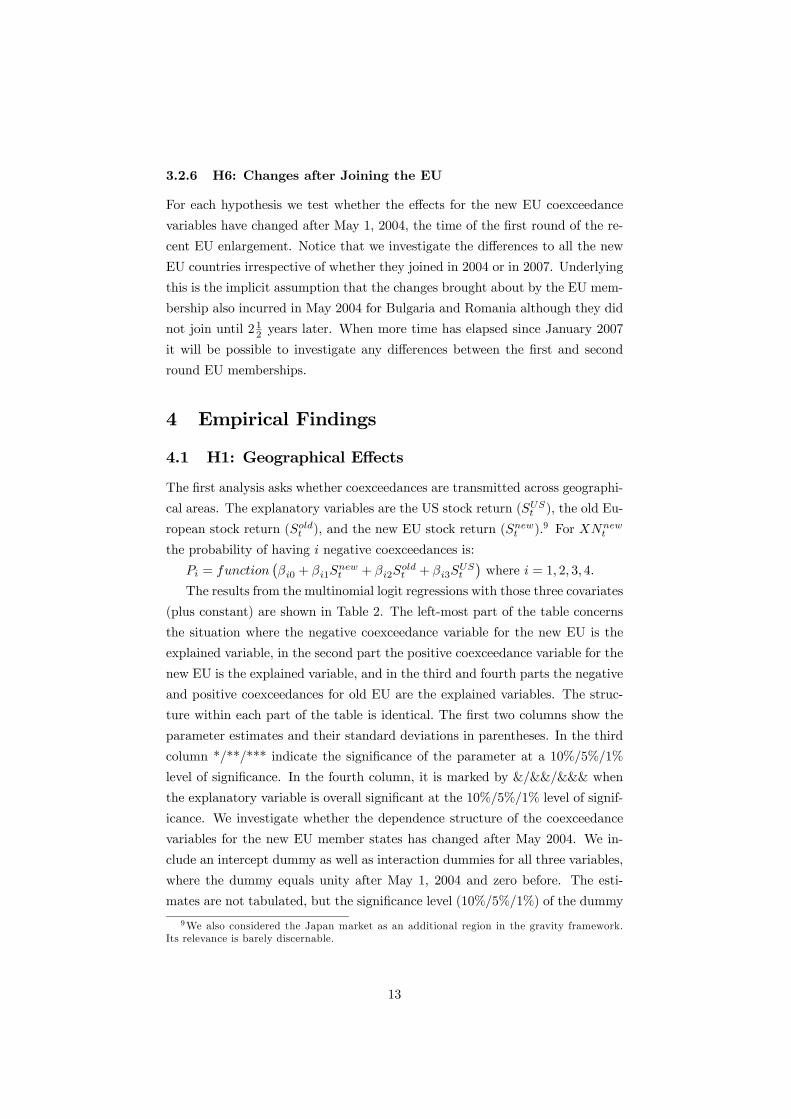
3.2.6 H6: Changes after Joining the EU

For each hypothesis we test whether the effects for the new EU coexceedance

variables have changed after May 1, 2004, the time of the first round of the re-

cent EU enlargement. Notice that we investigate the differences to all the new

EU countries irrespective of whether they joined in 2004 or in 2007. Underlying

this is the implicit assumption that the changes brought about by the EU mem-

bership also incurred in May 2004 for Bulgaria and Romania although they did

not join until 212 years later. When more time has elapsed since January 2007

it will be possible to investigate any differences between the first and second

round EU memberships.

4 Empirical Findings

4.1 H1: Geographical Effects

The first analysis asks whether coexceedances are transmitted across geographi-

cal areas. The explanatory variables are the US stock return (SUSt ), the old Eu-

ropean stock return (Soldt ), and the new EU stock return (Snewt ).9 For XNnewt

the probability of having i negative coexceedances is:

Pi = function¡βi0 + βi1S

newt + βi2S

oldt + βi3S

USt

¢where i = 1, 2, 3, 4.

The results from the multinomial logit regressions with those three covariates

(plus constant) are shown in Table 2. The left-most part of the table concerns

the situation where the negative coexceedance variable for the new EU is the

explained variable, in the second part the positive coexceedance variable for the

new EU is the explained variable, and in the third and fourth parts the negative

and positive coexceedances for old EU are the explained variables. The struc-

ture within each part of the table is identical. The first two columns show the

parameter estimates and their standard deviations in parentheses. In the third

column */**/*** indicate the significance of the parameter at a 10%/5%/1%

level of significance. In the fourth column, it is marked by &/&&/&&& when

the explanatory variable is overall significant at the 10%/5%/1% level of signif-

icance. We investigate whether the dependence structure of the coexceedance

variables for the new EU member states has changed after May 2004. We in-

clude an intercept dummy as well as interaction dummies for all three variables,

where the dummy equals unity after May 1, 2004 and zero before. The esti-

mates are not tabulated, but the significance level (10%/5%/1%) of the dummy

9We also considered the Japan market as an additional region in the gravity framework.Its relevance is barely discernable.

13

variables is indicated by #/##/### in the right-most column in the first two

parts of the table, i.e. in the regressions concerning the new EU.

For the negative coexceedances both for the new and old EU (XNnewt

and XNoldt ) we find that stock returns from all three regions are significant

in explaining the number of negative coexceedances, that is from western Eu-

rope, eastern Europe, and the US. The positive coexceedances for the new EU

(XPnewt ) is only influenced by its own stock market (Snewt ). The positive co-

exceedance for the old EU (XP oldt ) is influenced by both its own stock return

and the US stock return supporting the "gravity" hypothesis, cf. Rose (2000).

In general, for the negative coexceedance variables the influence from the stock

returns is negative, so that when stock returns are small, negative coexceedance

is more probable. The opposite applies for the positive coexceedance case.

For the negative coexceedance variable for the new EU member states only

the level has changed whereas the dependence of neither of the explained vari-

ables has changed (neither individually nor jointly). The probability of co-

exceedance has decreased after May 2004. Exactly the same applies to the

positive coexceedance variable for the new EU member states. The result is

somewhat surprising as we would have expected increased dependence on the

western European stock markets and higher synchronism among new member

states. However, it is arguable whether the prospect of a common currency is

synonymous with financial market integration and how long time is needed to

achieve it. Interestingly, Rogers (2007) shows that most of the substantial re-

duction in the dispersion of traded-goods prices across European cities occurred

between 1990 and 1994, i.e. the period of the "single market" initiative, rather

than after the introduction of euro. In the same line of reasoning, it is possi-

ble that interdependence between new and old member states was in progress

long before the formal enlargement in 2004 and that the convergence to the

Maastricht criteria had some effects before the formal adhesion date.

4.2 H2: Asset Class Effects

Now we ask whether coexceedances spill over across different assets types. The

explanatory variables are currency return (Ct), interest rate (Rt), and the old

European stock return (Soldt ). For XNnewt the probability of having i negative

coexceedances is:

Pi = function¡βi0 + βi1Ct + βi2Rt + βi3S

oldt

¢where i = 1, 2, 3, 4.

The results are given in Table 3. The table is structured as Table 2.10

10We are aware that some new EU members have relatively developed bond markets, e.g.Poland and Czech Republic. However, the limited number of these countries and their short

14

The results are robust to using the yield to maturity of the German 10-year

government bond index in place of the EURIBOR interest rates (results not

tabulated). So the results do not depend on whether we use a short term

interest rate or a long term interest rate.

For the negative coexceedance variable for the new EU member states only

the stock market has significant influence. The effect is negative as also found

when investigating the geographical effects. For the positive coexceedance vari-

able for the new EU member states both the currency return and the stock

return have a significant and positive influence. For the stock market this result

is in accordance with the findings regarding geographical effects. In neither case

for the new EU is the interest rate of importance.

For the old EU member states the negative coexceedance variable is influ-

enced by the currency return and the stock return, in both cases a negative

influence. For the positive coexceedance variable for the old EU all three vari-

ables are significant, a negative influence from the interest rate and a positive

influence from the currency return and the stock return. The signs of the in-

terest rate coefficients are in line with the discounted value approach, that is

an equity asset value decreases as its discounted factor increases. The relation

between coexceedance and currency movements can be interpreted in the light

of the standard models involving a central bank reaction function having a pref-

erence for low inflation. In this view, a more tightening monetary policy is the

response to some inflation concern that, in turn, appreciates the euro and it

overall dampens equity prices.

The fact that asset classes appear more highly interconnected in old than

new EU member states can be explained by a stronger market integration in

developed markets or, conversely, some market segmentation among investment

categories in new EU member states.

For the negative coexceedance variable for the new EU the influence of the

currency return changed after May 2004, when the influence became stronger

(more negative). The same applies to the stock return. Also the level decreased

after May 2004. For the positive coexceedance variable for the new EU only

the level changed after May 2004, when it decreased. At least for negative

coexceedances, this could be interpreted as an effect of the inclusion in the EU.

If the euro appreciates in response to a tighter monetary policy, this would

increase the likelihood of equity price falls in new EU member states after 2004

being all simultaneously affected by the euro’s fortune. This reaction would

be even more intense because of the Balassa-Samuelson effect, where inflation

lifetime do not allow a comprehensive analysis.

15

risk is higher for new EU states. On the other hand, it is worth emphasizing

that in the euro-zone there were two distinct monetary policy phases before and

after 2004. The former (latter) period was characterized by an expansionary

(restrictive) stance. In that sense, it is more likely to observe equity price drops

as euro appreciates after 2004.

4.3 H3: Volatility Effects

We investigate whether volatility factors can explain the occurrence of simulta-

neous very large or very small returns. We apply both currency, interest rate,

and stock market volatility as explanatory variables: σCt , σRt , and σoldt . For

XNnewt the probability of having i negative coexceedances is:

Pi = function¡βi0 + βi1σ

Ct + βi2σ

Rt + βi3σ

oldt

¢where i = 1, 2, 3, 4.

The results are given in Table 4. The table is structured as Table 2.

We also investigate this hypothesis using the volatility from the yield from

the German 10-year government index calculated as for the EURIBOR volatility

(results not tabulated). The results are consistent with what we find using the

ERIBOR volatility.

For the negative coexceedance variable for the new EU member states we

find that the stock market volatility acts as expected, i.e. the likelihood of

coexceedance increases in highly volatile environments, whereas the currency

volatility is insignificant. For the positive coexceedance variable for the new

EU member states we find that all three volatility factors are of significance.

The influence from stock volatility and currency volatility is mainly positive

as expected. The new EU coexceedances (both positive and negative) depend

negatively on the interest rate volatility, so that the more volatile the short

rate is, the less likely is the occurrence of coexceedances. This result supports

the idea that a larger change in EURIBOR rates is a sign of well-defined phase

of monetary stance and, in turn, it stands for less uncertainty coming from

monetary policy.

For the old EU member states the results are identical to those of the new

EU countries except that the positive coexceedance variable does not depend

on the currency volatility.

For the negative coexceedance variable for the new EU the probabilities have

changed after May 2004. The level has become smaller, such that negative coex-

ceedances have become less likely. Also, the dependence on the stock volatility

has increased. In contrast, for the positive coexceedance variable for the new

EU member states, the dependence structure on the volatilities has not changed

after May 2004. These findings can partially be explained by the equity bull

16

phase coupled with low volatility in recent years. An additional explanation is

that the new EU countries’ equity markets have become more connected with

old EU equity markets.

4.4 H4: Persistence Effects

We test whether the coexceedances are influenced by coexceedances of the same

type in the other European markets and whether the coexceedances are autore-

gressive. So for the negative coexceedance variable for the new EU member

states (XNnewt ) the explanatory variables are XNnew

t−1 and XNoldt . For XNnew

t

the probability of having i negative coexceedances is:

Pi = function¡βi0 + βi1XNnew

t−1 + βi2XNoldt

¢where i = 1, 2, 3, 4.

For all four regressions both explanatory variables are significant and the

influence is positive. So, the more extreme negative returns we have on the old

EU markets, the more likely it is to have many extreme negative returns on

the new EU markets. Moreover, the number of extreme negative returns today

is positively dependent on the number of extreme negative returns yesterday

supporting the "continuation" rather than the "reversal" hypothesis. A similar

interpretation applies to the other markets. The results are given in Table 5.

The table is structured as Table 2.

For the negative coexceedance variable for the new EU, the dependence

on the old EU has become stronger after May 2004. It appears that nothing

happens to the positive coexceedance variable for the new EU.11

We also considered other possible combinations such as adding positive co-

exceedances for the old EU markets (XP oldt ) to the equation for XNnew

t . This

opposite market movements would be reasonable in the light of flight to quality

effects when investors flee away from emerging markets to safer and more liquid

markets in times of stress. The results do not support this idea, in that XP oldt

is insignificant whereas XNoldt remains significant.

4.5 H5: Asymmetry Effects

The separate analysis of joint price drops and price jumps suggests that there

are significant differences between negative and positive coexceedances. In gen-

eral, negative coexceedances appear to be more dependent on the international

dynamics of stock markets. In contrast, positive coexceedances appear to be

more responsive to other asset classes, in particular with respect to the currency

movements both in terms of returns and volatility. Instead, the way positive and

11We do not include the term XP oldt multiplied by the May 2004 dummy, since we then get

a singular matrix.

17

negative coexceedances materialize in terms of persistence and interconnection

between old and new EU member states is similar.

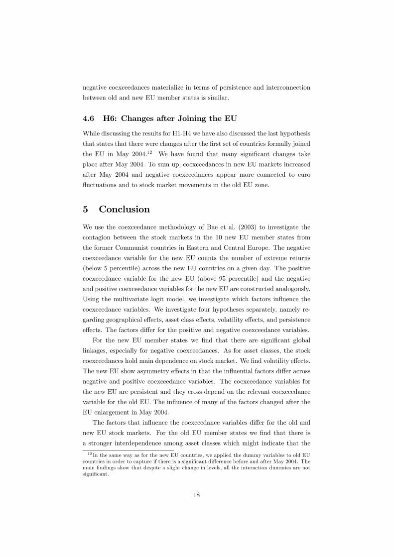
4.6 H6: Changes after Joining the EU

While discussing the results for H1-H4 we have also discussed the last hypothesis

that states that there were changes after the first set of countries formally joined

the EU in May 2004.12 We have found that many significant changes take

place after May 2004. To sum up, coexceedances in new EU markets increased

after May 2004 and negative coexceedances appear more connected to euro

fluctuations and to stock market movements in the old EU zone.

5 Conclusion

We use the coexceedance methodology of Bae et al. (2003) to investigate the

contagion between the stock markets in the 10 new EU member states from

the former Communist countries in Eastern and Central Europe. The negative

coexceedance variable for the new EU counts the number of extreme returns

(below 5 percentile) across the new EU countries on a given day. The positive

coexceedance variable for the new EU (above 95 percentile) and the negative

and positive coexceedance variables for the new EU are constructed analogously.

Using the multivariate logit model, we investigate which factors influence the

coexceedance variables. We investigate four hypotheses separately, namely re-

garding geographical effects, asset class effects, volatility effects, and persistence

effects. The factors differ for the positive and negative coexceedance variables.

For the new EU member states we find that there are significant global

linkages, especially for negative coexceedances. As for asset classes, the stock

coexceedances hold main dependence on stock market. We find volatility effects.

The new EU show asymmetry effects in that the influential factors differ across

negative and positive coexceedance variables. The coexceedance variables for

the new EU are persistent and they cross depend on the relevant coexceedance

variable for the old EU. The influence of many of the factors changed after the

EU enlargement in May 2004.

The factors that influence the coexceedance variables differ for the old and

new EU stock markets. For the old EU member states we find that there is

a stronger interdependence among asset classes which might indicate that the

12 In the same way as for the new EU countries, we applied the dummy variables to old EUcountries in order to capture if there is a significant difference before and after May 2004. Themain findings show that despite a slight change in levels, all the interaction dummies are notsignificant.

18

capital markets in the old EU are more integrated than in the new EU. We find

that the coexceedance variables for the old EU is persistent and that it cross

depends on the relevant coexceedance variable for the new EU. So the cross

dependence structure goes both ways, i.e. from old to new EU and from new to

old EU.

In future research it would be interesting to extend this method to analyze

coexceedance in other asset classes such as bonds, individual stocks, and hedge

funds, as well as in times of crucial changes of market conditions or monetary

regimes.

19

References

Adjaouté, K. and Danthine, J.-P.: 2003, European Financial Integration and

Equity Returns: A Theory-Based Assessment, in V. Gaspar, P. Hartmann

and O. Sleijpen (eds), The Transformation of the European Financial Sys-

tem, European Central Bank, Frankfurt, Germany, pp. 185—245.

Adjaouté, K. and Danthine, J.-P.: 2004, Equity Returns and Integration: Is

Europe Changing?, Oxford Review of Economic Policy 20(4), 555—570.

Bae, K.-H., Karolyi, G. A. and Stulz, R. M.: 2003, A New Approach to Mea-

suring Financial Contagion, Review of Financial Studies 16(3), 717—763.

Baig, T. and Goldfajn, I.: 1999, Financial Market Contagion in the Asian Crisis,

IMF Staff Papers 46(2).

Bank for International Settlements: 1999, International Banking and Financial

Market Developments, BIS Quarterly Review.

Bertero, E. and Mayer, C.: 1990, Structure and Performance: Global Interde-

pendence of Stock Markets around the Crash of October 1987, European

Economic Review 34(6), 1155—80.

Boyer, B. H., Gibson, M. and Loretan, M.: 1999, Pitfalls in Tests for Changes

in Correlation, Working paper, Board of Governors of the Federal Reserve

System.

Brunnermeier, M. K. and Pedersen, L. H.: 2007, Market Liquidity and Funding

Liquidity, Working Paper 12939, National Bureau of Economic Research.

Caballero, R. J. and Krishnamurthy, A.: 2007, Collective Risk Management in

a Flight to Quality Episode, Working Paper 12896, National Bureau of

Economic Research.

Calvo, G. A., Leiderman, L. and Reinhart, C. M.: 1996, Inflows of Capital

to Developing Countries in the 1990s, Journal of Economic Perspectives

10, 123—39.

Cappiello, L., Gérard, B., Kadareja, A. and Manganelli, S.: 2006, Financial

Integration of New EU Member States, Working Paper, European Central

Bank.

Chan-Lau, J. A., Methieson, D. J. and Yao, J. Y.: 2004, Extreme Contagion in

Equity Markets, Working Paper, International Monetary Fund.

20

Cox, D. R. and Peterson, D. R.: 1994, Stock Returns Following Large One-

Day Declines: Evidence on Short-Term Reversals and Longer-Term Perfor-

mance, Journal of Finance 49(1), 255—67.

Cumperayot, P., Keijzer, T. and Kouwenberg, R.: 2006, Linkages between Ex-

treme Stock Market and Currency Returns, Journal of International Money

and Finance 25, 528—550.

DeBond, W. F. M. and Thaler, R. H.: 1985, Does the Stock Market Overreact?,

Journal of Finance 40(3), 793—805.

Dovak, T.: 2007, Are the New and Old EU Countries Financially Integrated,

Journal of European Integration 29.

Dovak, T. and Podpiera, R.: 2006, European Union Enlargement and Equity

Markets in Accession Countries, Emerging Markets Review 7, 129—146.

Fazio, G.: forthcoming, Extreme Interdependence and Extreme Contagion Be-

tween Emergin Markets, Journal of International Money and Finance .

Forbes, K. and Rigobon, R.: 2002, No Contagion, Only Interdependence: Mea-

suring Stock Market Comovements, Journal of Finance 57, 2223—2262.

Hartmann, P., Straetmans, S. and de Vries, C. G.: 2004, Asset Market Linkages

in Crisis Periods, Review of Economics and Statistics 86(1), 313—326.

King, M. A. and Wadhwani, S.: 1990, Transmission of Volatility between Stock

Markets, Review of Financial Studies 3(1), 5—33.

Moore, T. and Wang, P.: 2007, Volatility in Stock Returns for New EU Member

States: Markow Regime Switching Model, International Review of Finan-

cial Analysis 16, 282—292.

Morris, S. and Shin, H. S.: 1998, Unique Equilibrium in a Model of Self-Fulfilling

Currency Attacks, American Economic Review 88(3), 587—97.

Mundell, R. A.: 1961, A Theory of Optimum Currency Areas, American Eco-

nomic Review 51(4), 657—665.

Obstfeld, M.: 1986, Rational and Self-Fulfilling Balance-of-Payments Crises,

American Economic Review 76, 72—81.

Rogers, J. H.: 2007, Monetary Union, Price Level Convergence, and Infla-

tion: How Close is Europe to the USA?, Journal of Monetary Economics

54(3), 785—796.

21

Rose, A. K.: 2000, One Money, One Market? The Effects of Common Currencies

on International Trade, Economic Policy 15, 7—46.

Samitas, A., Kenourgios, D. and Paltalidis, N.: 2007, Financial Crises and Stock

Market Dependence, Working paper, EFMA Annual Meeting.

Schinasi, G. J. and Smith, R.: 2001, Portfolio Diversification, Leverage, and

Financial Contagion, in S. Claessens and K. Forbes (eds), International

Financial Contagion, Kluwer Academic Publishers, Boston MA, pp. 187—

223.

22

Table 1: Summary Statistics

0 1 2 3 4+

Positive CoexceedancesNew EU East 1090 (64%) 429 (25%) 133 (8%) 50 (3%) 8 (0.5%)Old EU 1296 (76%) 206 (12%) 56 (3%) 27 (2%) 125 (7%)

Negative CoexceedancesNew EU East 1130 (66%) 369 (22%) 123 (7%) 44 (3%) 44 (3%)Old EU 1320 (77%) 176 (10%) 48 (3%) 28 (2%) 138 (8%)

Number of Coexceedances

23

Table 2: Geographical Effects

Constant(1) -1.10 (0.06) *** &&& ### -1.00 (0.06) *** &&& ### -2.02 (0.08) *** &&& -1.85 (0.08) *** &&&

Constant(2) -2.24 (0.10) *** -2.28 (0.11) *** -3.63 (0.19) *** -3.40 (0.17) ***

Constant(3) -3.63 (0.20) *** -3.91 (0.23) *** -4.20 (0.25) *** -4.41 (0.27) ***

Constant(4) -4.09 (0.24) *** -6.17 (0.60) *** -3.13 (0.15) *** -3.34 (0.16) ***

Snew(1) -0.28 (0.06) *** &&& # 0.34 (0.06) *** &&& -0.19 (0.08) ** &&& 0.05 (0.08)

Snew(2) -0.52 (0.10) *** 0.68 (0.10) *** -0.59 (0.13) *** 0.21 (0.13)

Snew(3) -0.74 (0.15) *** 1.32 (0.16) *** -0.48 (0.17) *** -0.02 (0.19)

Snew(4) -1.18 (0.15) *** 1.57 (0.30) *** -0.20 (0.10) ** 0.12 (0.10)

Sold(1) -0.06 (0.08) &&& 0.06 (0.07) -0.60 (0.11) *** &&& 0.31 (0.10) *** &&&

Sold

(2) -0.21 (0.12) * 0.11 (0.12) -0.76 (0.19) *** 0.62 (0.20) ***

Sold

(3) -0.50 (0.17) *** -0.32 (0.20) -0.95 (0.24) *** 1.45 (0.25) ***

Sold

(4) -0.59 (0.16) *** -0.01 (0.41) -1.64 (0.14) *** 1.69 (0.15) ***

SUS

(1) -0.16 (0.07) ** && -0.11 (0.07) -0.15 (0.09) &&& 0.10 (0.09) &&&

SUS

(2) 0.06 (0.11) 0.02 (0.10) -0.32 (0.15) ** 0.44 (0.15) ***

SUS(3) -0.20 (0.16) -0.06 (0.17) -0.31 (0.19) 0.09 (0.20)

SUS(4) 0.21 (0.15) 0.03 (0.30) -0.40 (0.11) *** 0.32 (0.11) ***

Pseudo R-square

Chi-square

Positive CoexceedancesNew EU

Negative CoexceedancesOld EU

Positive CoexceedancesNegative Coexceedances

0.07226.2***

0.05170.9***

0.16

434.1*** 321.3***0.11

The table shows the parameter estimates arising from estimating the multinomial logit model

for the negative coexceedance variable for the new EU (first part of the table), the positive

coexceedance variable for the new EU (second part of the table), the negative coexceedances

for the old EU (third part of the table), and the positive coexceedances for the old EU (fourth

part of the table). Standard errors in parentheses. */**/*** indicate that the parameter is

significantly different from zero at 10%/5%/1% level. &/&&/&&& indicate that the explana-

tory variable is significant at 10%/5%/1% level. #/##/### indicate that the parameter is

significantly different after May 2004 at 10%, 5%, and 1% level.

24

Table 3: Asset Class Effects

Constant(1) -1.11 (0.06) *** &&& ### -0.98 (0.06) *** &&& ### -2.03 (0.08) *** &&& -1.84 (0.08) *** &&&

Constant(2) -2.23 (0.10) *** -2.17 (0.10) *** -3.60 (0.18) *** -3.40 (0.17) ***Constant(3) -3.51 (0.18) *** -3.25 (0.16) *** -4.23 (0.25) *** -4.46 (0.28) ***Constant(4) -3.64 (0.20) *** -5.36 (0.46) *** -3.22 (0.15) -3.46 (0.17) ***C(1) -0.18 (0.11) * ### -0.02 (0.10) &&& -0.36 (0.15) ** &&& 0.17 (0.14) &&&

C(2) -0.05 (0.17) 0.49 (0.16) *** -0.97 (0.26) *** 0.96 (0.24) ***C(3) -0.23 (0.26) -0.19 (0.27) -0.82 (0.34) ** 0.76 (0.34) **C(4) -0.08 (0.26) 1.28 (0.55) ** -1.16 (0.19) *** 1.19 (0.19) ***R(1) 0.00 (1.18) 0.29 (1.11) 0.46 (1.71) 2.27 (1.34) * &&&

R(2) -1.50 (1.75) -2.56 (1.63) -2.36 (2.43) -1.61 (3.03)R(3) -2.59 (2.24) -0.70 (2.91) -5.09 (2.02) ** -1.32 (3.68)R(4) 0.81 (3.26) 1.53 (5.63) -1.57 (1.92) -5.91 (1.94) ***

Sold(1) -0.28 (0.07) *** &&& ### 0.15 (0.06) ** &&& # -0.83 (0.11) *** &&& 0.40 (0.10) *** &&&

Sold(2) -0.40 (0.10) *** 0.47 (0.10) *** -1.38 (0.18) *** 1.16 (0.19) ***

Sold(3) -0.94 (0.14) *** 0.21 (0.17) -1.46 (0.22) *** 1.67 (0.24) ***

Sold(4) -1.08 (0.13) *** 0.82 (0.30) *** -2.09 (0.14) *** 2.15 (0.16) ***Pseudo R-squareChi-square 445.4*** 364.0***

Old UNegative Coexceedances Positive Coexceedances

0.16 0.13

Negative Coexceedances

0.03110.3***

New EU

0.0144.7***

Positive Coexceedances








significantly different after May 2004 at 10%/5%/1% level.

25

Table 4: Volatility Effects

Constant(1) -1.54 (0.45) *** &&& ## 0.14 (0.44) &&& -3.07 (0.61) *** &&& -2.88 (0.57) *** &&&

Constant(2) -4.52 (0.71) *** -2.00 (0.67) *** -5.29 (1.14) *** -4.67 (1.01) ***Constant(3) -5.84 (1.14) *** -4.44 (1.14) *** -6.31 (1.41) *** -7.33 (1.51) ***Constant(4) -5.70 (1.17) *** -9.27 (2.79) *** -4.38 (0.69) *** -3.84 (0.71) ***σC(1) 0.19 (0.70) & -2.21 (0.69) *** && 0.79 (0.91) 0.78 (0.87)

σC(2) 2.78 (1.06) *** -1.01 (1.04) 3.60 (1.52) ** 1.50 (1.53)

σC(3) 2.56 (1.73) 1.65 (1.69) 1.51 (2.15) 3.82 (2.09) *σC(4) 0.61 (1.88) 2.95 (4.28) 0.65 (1.04) -0.58 (1.10)

σR(1) -4.32 (1.84) ** && -4.30 (1.56) *** &&& -10.44 (3.56) *** &&& -1.94 (2.18) &&

σR(2) -2.39 (3.31) -8.66 (3.37) ** -46.55 (17.90) *** -3.57 (4.63)

σR(3) 1.71 (4.31) -7.60 (6.62) -3.65 (6.78) -21.10 (16.96)

σR(4) 5.82 (3.32) * 9.85 (7.73) -10.82 (4.37) ** -14.21 (5.08) ***

σold(1) 0.49 (0.18) *** &&& ## 0.33 (0.17) * &&& # 0.94 (0.23) *** &&& 0.71 (0.22) *** &&&

σold(2) 0.77 (0.25) *** 0.81 (0.23) *** 0.67 (0.41) * 0.82 (0.37) **

σold(3) 1.07 (0.36) *** 0.47 (0.40) 1.72 (0.42) *** 1.55 (0.42) ***σold(4) 1.85 (0.33) *** 2.05 (0.67) *** 2.00 (0.21) *** 2.14 (0.22) ***Pseudo R-squareChi-square

New EU Old UNegative Coexceedances Positive Coexceedances Negative Coexceedances Positive Coexceedances

0.02 0.02 0.07 0.0677.5** 51.8*** 197.7*** 161.5***









26

Table 5: Persistence Effects

Constant(1) -1.41 (0.08) *** &&& -1.12 (0.07) *** &&& ## -2.34 (0.10) *** &&& -2.11 (0.10) *** &&&

Constant(2) -2.64 (0.13) *** -2.58 (0.13) *** -4.04 (0.21) *** -3.61 (0.19) ***Constant(3) -4.75 (0.29) *** -4.12 (0.25) *** -4.38 (0.26) *** -4.38 (0.28) ***Constant(4) -4.94 (0.31) *** -5.06 (0.47) *** -3.42 (0.15) *** -2.78 (0.13) ***Own Lagged(1) 0.27 (0.07) *** &&& 0.17 (0.07) ** &&& 0.15 (0.07) ** &&& 0.25 (0.06) *** &&&

Own Lagged(2) 0.35 (0.09) *** 0.45 (0.10) *** 0.31 (0.10) *** 0.31 (0.10) ***Own Lagged(3) 0.71 (0.13) *** 0.80 (0.14) *** 0.29 (0.13) ** 0.39 (0.13) ***Own Lagged(4) 0.69 (0.13) *** -0.12 (0.53) 0.39 (0.06) *** 0.26 (0.07) ***Opposite(1) 0.33 (0.05) *** &&& ## 0.12 (0.05) ** &&& NA 0.47 (0.09) *** &&& 0.24 (0.09) *** &&&

Opposite(2) 0.42 (0.07) *** 0.36 (0.07) *** 0.76 (0.12) *** 0.45 (0.14) ***Opposite(3) 0.89 (0.09) *** 0.43 (0.10) *** 0.57 (0.18) *** 0.40 (0.21) **Opposite(4) 0.97 (0.10) *** 0.29 (0.25) 0.99 (0.08) *** 0.47 (0.10) ***Pseudo R-squareChi-square

New EU Old UNegative Coexceedances Positive Coexceedances Negative Coexceedances Positive Coexceedances

0.08 0.02 0.09 0.02262.9*** 75.5*** 254.6*** 70.8***









27

XN new

0

1

2

3

4

2000-10-02

2000-11-17

2001-01-04

2001-02-21

2001-04-10

2001-05-28

2001-07-13

2001-08-30

2001-10-17

2001-12-04

2002-01-21

2002-03-08

2002-04-25

2002-06-12

2002-07-30

2002-09-16

2002-11-01

2002-12-19

2003-02-05

2003-03-25

2003-05-12

2003-06-27

2003-08-14

2003-10-01

2003-11-18

2004-01-05

2004-02-20

2004-04-08

2004-05-26

2004-07-13

2004-08-30

2004-10-15

2004-12-02

2005-01-19

2005-03-08

2005-04-25

2005-06-10

2005-07-28

2005-09-14

2005-11-01

2005-12-19

2006-02-03

2006-03-23

2006-05-10

2006-06-27

2006-08-14

2006-09-29

2006-11-16

2007-01-03

2007-02-20

2007-04-09

Figure 1: Time Series Plot of the Negative Coexceedance Variable for the New

EU

XP new

0

1

2

3

4

2000-10-02

2000-11-17

2001-01-04

2001-02-21

2001-04-10

2001-05-28

2001-07-13

2001-08-30

2001-10-17

2001-12-04

2002-01-21

2002-03-08

2002-04-25

2002-06-12

2002-07-30

2002-09-16

2002-11-01

2002-12-19

2003-02-05

2003-03-25

2003-05-12

2003-06-27

2003-08-14

2003-10-01

2003-11-18

2004-01-05

2004-02-20

2004-04-08

2004-05-26

2004-07-13

2004-08-30

2004-10-15

2004-12-02

2005-01-19

2005-03-08

2005-04-25

2005-06-10

2005-07-28

2005-09-14

2005-11-01

2005-12-19

2006-02-03

2006-03-23

2006-05-10

2006-06-27

2006-08-14

2006-09-29

2006-11-16

2007-01-03

2007-02-20

2007-04-09

Figure 2: Time Series Plot of the Positive Coexceedance Variable for the New

EU

28

XN old

0

1

2

3

4

2000-10-02

2000-11-17

2001-01-04

2001-02-21

2001-04-10

2001-05-28

2001-07-13

2001-08-30

2001-10-17

2001-12-04

2002-01-21

2002-03-08

2002-04-25

2002-06-12

2002-07-30

2002-09-16

2002-11-01

2002-12-19

2003-02-05

2003-03-25

2003-05-12

2003-06-27

2003-08-14

2003-10-01

2003-11-18

2004-01-05

2004-02-20

2004-04-08

2004-05-26

2004-07-13

2004-08-30

2004-10-15

2004-12-02

2005-01-19

2005-03-08

2005-04-25

2005-06-10

2005-07-28

2005-09-14

2005-11-01

2005-12-19

2006-02-03

2006-03-23

2006-05-10

2006-06-27

2006-08-14

2006-09-29

2006-11-16

2007-01-03

2007-02-20

2007-04-09

Figure 3: Time Series Plot of the Negative Coexceedance Variable for the Old

EU

XP old

0

1

2

3

4

2000-10-02

2000-11-17

2001-01-04

2001-02-21

2001-04-10

2001-05-28

2001-07-13

2001-08-30

2001-10-17

2001-12-04

2002-01-21

2002-03-08

2002-04-25

2002-06-12

2002-07-30

2002-09-16

2002-11-01

2002-12-19

2003-02-05

2003-03-25

2003-05-12

2003-06-27

2003-08-14

2003-10-01

2003-11-18

2004-01-05

2004-02-20

2004-04-08

2004-05-26

2004-07-13

2004-08-30

2004-10-15

2004-12-02

2005-01-19

2005-03-08

2005-04-25

2005-06-10

2005-07-28

2005-09-14

2005-11-01

2005-12-19

2006-02-03

2006-03-23

2006-05-10

2006-06-27

2006-08-14

2006-09-29

2006-11-16

2007-01-03

2007-02-20

2007-04-09

Figure 4: Time Series Plot of the Positive Coexceedance Variable for the Old

EU

29

Extreme Coexceedances in New EU Member States’ Stock Markets

Documents