Tiago Manuel Jesus Carvalho Bachelor degree in Chemical and Biochemical Engineering Extraction of raw plant material using supercritical carbon dioxide Dissertation submitted in partial fulfillment of the requirements for the degree of Master of Science in Chemical and Biochemical Engineering Adviser: Ewa Bogel-Lukasik, Auxiliary Researcher, Faculdade de Ciências e Tecnologia da Universidade Nova de Lisboa Co-adviser: Marek Henczka, Vice-Dean for Academic Affairs, Warsaw University of Technology, Faculty of Chemical and Process Engineering Examination Committee Chairperson: Maria Madalena Alves Campos de Sousa Dionísio Andrade Members: Ana Vital Morgado Nunes Ewa Bogel-Lukasik November, 2016

Welcome message from author
This document is posted to help you gain knowledge. Please leave a comment to let me know what you think about it! Share it to your friends and learn new things together.
Transcript

Tiago Manuel Jesus Carvalho
Bachelor degree in Chemical and Biochemical Engineering
Extraction of raw plant material usingsupercritical carbon dioxide
Dissertation submitted in partial fulfillmentof the requirements for the degree of
Master of Science inChemical and Biochemical Engineering
Adviser: Ewa Bogel-Lukasik, Auxiliary Researcher,Faculdade de Ciências e Tecnologia da UniversidadeNova de Lisboa
Co-adviser: Marek Henczka, Vice-Dean for Academic Affairs,Warsaw University of Technology, Faculty of Chemicaland Process Engineering
Examination Committee
Chairperson: Maria Madalena Alves Campos de Sousa Dionísio AndradeMembers: Ana Vital Morgado Nunes
Ewa Bogel-Lukasik
November, 2016


Extraction of raw plant material using supercritical carbon dioxide
Copyright © Tiago Manuel Jesus Carvalho, Faculty of Sciences and Technology, NOVA
University of Lisbon.
The Faculty of Sciences and Technology and the NOVA University of Lisbon have the
right, perpetual and without geographical boundaries, to file and publish this dissertation
through printed copies reproduced on paper or on digital form, or by any other means
known or that may be invented, and to disseminate through scientific repositories and
admit its copying and distribution for non-commercial, educational or research purposes,
as long as credit is given to the author and editor.
This document was created using the (pdf)LATEX processor, based in the “unlthesis” template[1], developed at the Dep. Informática of FCT-NOVA [2].[1] https://github.com/joaomlourenco/unlthesis [2] http://www.di.fct.unl.pt


Acknowledgements
I would like first of all to thank my thesis advisor Ewa Bogel-Lukasik, auxiliary researcher
at Faculdade de Ciências e Tecnologia of Universidade Nova de Lisboa, for all the support
and for giving me strength in the most difficult moments. The door was always open
when I needed help or advice and for that I so grateful.
I would also like to thank professor Marek Henczka and Jan Krzysztoforski from the
faculty of Chemical and Process Engineering of the Warsaw University of Technology for
helping and supporting me in this six months. I arrived in a different country without
knowing what to expect and you made me feel at home.
Finally, I must express my very profound gratitude to my parents, family and friends
for providing me with unfailing support and continuous encouragement throughout my
years of study and through the process of researching and writing this thesis. I would
never be able to come so far without them. Thank you for everything.
Tiago Carvalho
v


Abstract
Many of the herbs and spices used by humans are important medicinal compounds.
The aim of this work is to investigate the extraction mechanisms of plant materials by
using supercritical fluid extraction (SFE). In order to do this, a supercritical extraction
system was designed and set-up allowing to use supercritical CO2 for the extraction of
raw plant material, such as Sassafras albidum and Berberis vulgaris.
The planned work found difficulties due to legal problems and the objective plant
material had to be changed for this reason. The first plant considered was Sassafras
albidum which later on was changed to Berberis vulgaris. Supercritical extraction in
dynamic and steady state were executed in order to study the extraction parameters and
attempt to recover a compound called berberine.
The results of the experiments show that supercritical fluid extraction is a sufficient
extraction method for the plant Berberis vulgaris. On the other hand, it was not possible
to apply any analytical methods to prove that berberine was obtained since the amount of
extract was not sufficient for the techniques available. Even so, physical properties such as
smell and yellow color of the extract suggested that berberine might have been extracted.
The whole designed supercritical extraction process needs improvements such as the
introduction of organic solvents to increase the extraction yield and the introduction
of an alternative analytical protocol such as High Performance Liquid Chromatography
(HPLC).
Keywords: Supercritical Fluid Extraction, safrole, berberine . . .
vii


Resumo
Vária ervas e especiarias usadas por humanos contêm compostos com propriedades
medicinais e em muitas partes do mundo acabam por ser a principal fonte de tratamento
médico. O objetivo deste trabalho consiste em investigar os mecanismos de extração de
plantas, usando para o efeito extração com fluidos supercríticos. Para esse efeito um
sistema de extração foi desenvolvido e montado de forma a usar CO2 supercrítico como
solvente para a extração da planta.
A estrutura deste trabalho pode parecer irregular uma vez que a planta alvo teve de
ser mudada por razões legais. A primeira planta a ser considerada foi Sassafras albidum
e depois foi alterada para Berberis vulgaris. As extrações usando fluidos supercríticos em
estado estacionário e dinâmico foram executadas de forma a estudar os parâmetros da
extração e tentar obter o composto alvo berberine.
Os resultados experimentais mostram que extração usando fluidos supercríticos é
efetiva na extração da planta Berberis vulgaris. Relativamente ao composto Berberine não
foi possível provar a sua extração, mas propriedades físicas manifestadas no extrato como
cheiro e cor amarela sugerem que o composto estava presente em pequena quantidade. É
também sugerido que o processo seja alvo de um maior desenvolvimento nomeadamente
introduzindo solventes orgânicos para aumentar o rendimento da extração ou introduzir
um método alternativo para análise do composto alvo como por exemplo cromatografia
líquida de alta eficiência.
Palavras-chave: Fluidos supercríticos, extração, berberine, safrole . . .
ix


Contents
List of Figures xiii
List of Tables xvii
1 Introduction 1
1.1 Motivation . . . . . . . . . . . . . . . . . . . . . . . . . . . . . . . . . . . . 1
1.2 Aim of the work . . . . . . . . . . . . . . . . . . . . . . . . . . . . . . . . . 2
2 Theoretical Background 3
2.1 Medicinal Plants . . . . . . . . . . . . . . . . . . . . . . . . . . . . . . . . . 3
2.2 Extraction Methods . . . . . . . . . . . . . . . . . . . . . . . . . . . . . . . 9
2.2.1 Conventional Extraction . . . . . . . . . . . . . . . . . . . . . . . . 9
2.2.1.1 Water Distillation . . . . . . . . . . . . . . . . . . . . . . 9
2.2.1.2 Steam Distillation . . . . . . . . . . . . . . . . . . . . . . 10
2.2.1.3 Organic Solvent Extraction . . . . . . . . . . . . . . . . . 12
2.2.1.4 Cold Pressing . . . . . . . . . . . . . . . . . . . . . . . . . 13
2.2.2 Green Extraction with Innovative Methods . . . . . . . . . . . . . 15
2.2.2.1 Subcritical Extraction . . . . . . . . . . . . . . . . . . . . 15
2.2.2.2 Ultrasound Assisted Extraction . . . . . . . . . . . . . . . 17
2.2.2.3 Microwave Assisted Extraction . . . . . . . . . . . . . . . 18
2.2.2.4 Supercritical Fluid Extraction . . . . . . . . . . . . . . . . 20
2.3 Supercritical Fluids . . . . . . . . . . . . . . . . . . . . . . . . . . . . . . . 23
2.4 Analytical Methods . . . . . . . . . . . . . . . . . . . . . . . . . . . . . . . 27
3 Safrole - Extraction and Reaction 33
3.1 Sassafras . . . . . . . . . . . . . . . . . . . . . . . . . . . . . . . . . . . . . 33
3.1.1 Sassafras Plant . . . . . . . . . . . . . . . . . . . . . . . . . . . . . . 33
3.1.2 Sassafras Oil . . . . . . . . . . . . . . . . . . . . . . . . . . . . . . . 35
3.2 Safrole . . . . . . . . . . . . . . . . . . . . . . . . . . . . . . . . . . . . . . 36
3.2.1 Safrole Oxide . . . . . . . . . . . . . . . . . . . . . . . . . . . . . . 37
3.3 Experimental Part . . . . . . . . . . . . . . . . . . . . . . . . . . . . . . . . 39
3.3.1 Solubility Parameters . . . . . . . . . . . . . . . . . . . . . . . . . . 39
3.3.2 Extraction . . . . . . . . . . . . . . . . . . . . . . . . . . . . . . . . 41
xi

CONTENTS
3.3.2.1 Steam Distillation . . . . . . . . . . . . . . . . . . . . . . 41
3.3.2.2 Supercritical Extraction . . . . . . . . . . . . . . . . . . . 43
3.3.3 Epoxidation Reaction . . . . . . . . . . . . . . . . . . . . . . . . . . 44
3.4 Proposed Analysis . . . . . . . . . . . . . . . . . . . . . . . . . . . . . . . . 47
4 Berberine - Sources and Extraction 49
4.1 Sources and Origins . . . . . . . . . . . . . . . . . . . . . . . . . . . . . . . 49
4.2 Experimental Part . . . . . . . . . . . . . . . . . . . . . . . . . . . . . . . . 52
4.2.1 Materials . . . . . . . . . . . . . . . . . . . . . . . . . . . . . . . . . 52
4.2.2 Supercritical Fluid Extraction Systems . . . . . . . . . . . . . . . . 52
4.2.2.1 Dynamic System . . . . . . . . . . . . . . . . . . . . . . . 53
4.2.2.2 Static System . . . . . . . . . . . . . . . . . . . . . . . . . 55
4.2.3 Extraction Process . . . . . . . . . . . . . . . . . . . . . . . . . . . . 56
4.2.3.1 Extraction in Dynamic Mode . . . . . . . . . . . . . . . . 56
4.2.3.2 Extraction in Static Mode . . . . . . . . . . . . . . . . . . 59
4.2.4 Water content . . . . . . . . . . . . . . . . . . . . . . . . . . . . . . 60
4.3 Analytical Method . . . . . . . . . . . . . . . . . . . . . . . . . . . . . . . . 61
5 Results and Discussion 63
6 Conclusions 85
Bibliography 89
A Table Results 97
xii

List of Figures
2.1 Water Distillation Apparatus . . . . . . . . . . . . . . . . . . . . . . . . . . . . 10
2.2 Steam Distillation Apparatus . . . . . . . . . . . . . . . . . . . . . . . . . . . 11
2.3 Vapor Distillation Apparatus . . . . . . . . . . . . . . . . . . . . . . . . . . . . 11
2.4 Soxhlet Extractor. . . . . . . . . . . . . . . . . . . . . . . . . . . . . . . . . . . 12
2.5 Cold Pressing apparatus. . . . . . . . . . . . . . . . . . . . . . . . . . . . . . . 14
2.6 Subcritical Water Extraction apparatus example has described above. . . . . 16
2.7 SFME apparatus. . . . . . . . . . . . . . . . . . . . . . . . . . . . . . . . . . . . 18
2.8 MHG apparatus. . . . . . . . . . . . . . . . . . . . . . . . . . . . . . . . . . . . 19
2.9 MSD apparatus. . . . . . . . . . . . . . . . . . . . . . . . . . . . . . . . . . . . 19
2.10 MSDf apparatus. . . . . . . . . . . . . . . . . . . . . . . . . . . . . . . . . . . . 20
2.11 Static Supercritical Extraction apparatus. . . . . . . . . . . . . . . . . . . . . . 21
2.12 Dynamic Supercritical Extraction apparatus. . . . . . . . . . . . . . . . . . . 21
2.13 Illustration of the critical point. . . . . . . . . . . . . . . . . . . . . . . . . . . 24
2.14 Representation of the various states until achieving a supercritical fluid. . . . 25
2.15 Gas Chromatography (GC) apparatus. . . . . . . . . . . . . . . . . . . . . . . 28
2.16 Example of GC output. . . . . . . . . . . . . . . . . . . . . . . . . . . . . . . . 29
2.17 Example of GC/MS output. . . . . . . . . . . . . . . . . . . . . . . . . . . . . 30
2.18 GC/MS apparatus . . . . . . . . . . . . . . . . . . . . . . . . . . . . . . . . . . 30
2.19 Example of an HPLC apparatus . . . . . . . . . . . . . . . . . . . . . . . . . . 31
2.20 Example of an DSC apparatus . . . . . . . . . . . . . . . . . . . . . . . . . . . 32
3.1 Sassafras albidum tree. . . . . . . . . . . . . . . . . . . . . . . . . . . . . . . . 34
3.2 Sassafras oil. . . . . . . . . . . . . . . . . . . . . . . . . . . . . . . . . . . . . . 35
3.3 Root beer, one of the past main applications for Sassafras oil. . . . . . . . . . 36
3.4 Main safrole application today: Ecstasy . . . . . . . . . . . . . . . . . . . . . . 37
3.5 Safrole Oxide Structure . . . . . . . . . . . . . . . . . . . . . . . . . . . . . . . 37
3.6 Epoxidation of safrole using MCPBA has an oxidizing agent. . . . . . . . . . 38
3.7 mCPBA Structure. . . . . . . . . . . . . . . . . . . . . . . . . . . . . . . . . . . 38
3.8 Scheme of the apparatus used for the steam distillation. . . . . . . . . . . . . 41
3.9 Sassafras albidum root bark. . . . . . . . . . . . . . . . . . . . . . . . . . . . . 42
3.10 Sassafras albidum root bark after steam distillation. . . . . . . . . . . . . . . 42
3.11 Oil obtained by steam distillation. . . . . . . . . . . . . . . . . . . . . . . . . . 43
xiii

List of Figures
3.12 Proposed apparatus for supercritical extraction. . . . . . . . . . . . . . . . . . 43
3.13 Isomerization reaction of safrole by catalyst action. . . . . . . . . . . . . . . . 45
3.14 Safrole epoxidation reaction. . . . . . . . . . . . . . . . . . . . . . . . . . . . . 45
3.15 Proposed epoxidation apparatus. . . . . . . . . . . . . . . . . . . . . . . . . . 46
3.16 Peroxycarbonic Acid Formation. . . . . . . . . . . . . . . . . . . . . . . . . . . 47
4.1 Berberis vulgaris tree. . . . . . . . . . . . . . . . . . . . . . . . . . . . . . . . . 50
4.2 Chemical Structure of Berberine. . . . . . . . . . . . . . . . . . . . . . . . . . 51
4.3 Exterior extraction vessel. . . . . . . . . . . . . . . . . . . . . . . . . . . . . . 53
4.4 Inner extraction vessel. . . . . . . . . . . . . . . . . . . . . . . . . . . . . . . . 53
4.5 Pressure control valve. . . . . . . . . . . . . . . . . . . . . . . . . . . . . . . . 54
4.6 Digital screens giving the values of temperature (oC) and pressure (bar). . . . 54
4.7 Design Dynamic Supercritical Extraction System. . . . . . . . . . . . . . . . . 54
4.8 Type of reactor used in static extraction. . . . . . . . . . . . . . . . . . . . . . 55
4.9 Oven for reactor temperature control. . . . . . . . . . . . . . . . . . . . . . . . 55
4.10 Analogic pressure indicator. . . . . . . . . . . . . . . . . . . . . . . . . . . . . 56
4.11 Example of non milled root bark. . . . . . . . . . . . . . . . . . . . . . . . . . 56
4.12 Example of milled material. . . . . . . . . . . . . . . . . . . . . . . . . . . . . 57
4.13 Serpentine used. . . . . . . . . . . . . . . . . . . . . . . . . . . . . . . . . . . . 58
4.14 Apparatus used for dynamic extraction. . . . . . . . . . . . . . . . . . . . . . 58
4.15 Bag containing plant material. . . . . . . . . . . . . . . . . . . . . . . . . . . . 59
4.16 Apparatus used for static extraction. . . . . . . . . . . . . . . . . . . . . . . . 60
4.17 Collection by depressurization. . . . . . . . . . . . . . . . . . . . . . . . . . . 60
4.18 Samples for analyzes of water content. . . . . . . . . . . . . . . . . . . . . . . 61
5.1 Cumulative Yield at 100 bar at 40oC (first experiment). . . . . . . . . . . . . 64
5.2 Cumulative Yield at 100 bar at 40oC (second experiment). . . . . . . . . . . . 65
5.3 Cumulative Yield at the conditions of 150 bar and 40oC (first experiment). . 66
5.4 Cumulative Yield at the conditions of 150 bar and 40oC (second experiment). 67
5.5 Cumulative Yield at the conditions of 200 bar and 40oC (first experiment). . 68
5.6 Cumulative Yield at the conditions of 200 bar and 40oC (second experiment). 69
5.7 Cumulative Yield at the conditions of 250 bar and 40oC (first experiment). . 70
5.8 Cumulative Yield at the conditions of 250 bar and 40oC (second experiment). 71
5.9 Comparison of the effect of different pressures at the temperature of 40oC. . 71
5.10 Cumulative Yield at the conditions of 70 bar and 60oC (first experiment). . . 72
5.11 Cumulative Yield at the conditions of 70 bar and 60oC (second experiment). 73
5.12 Cumulative Yield at the conditions of 100 bar and 60oC (first experiment). . 74
5.13 Cumulative Yield at the conditions of 100 bar and 60oC (second experiment). 75
5.14 Cumulative Yield at the conditions of 100 bar and 60oC (third experiment). . 76
5.15 Cumulative Yield at the conditions of 150 bar and 60oC (first experiment). . 77
5.16 Cumulative Yield at the conditions of 150 bar and 60oC (second experiment). 78
xiv

List of Figures
5.17 Cumulative Yield at the conditions of 150 bar and 60oC (third experiment). . 79
5.18 Cumulative Yield at the conditions of 200 bar and 60oC (first experiment). . 80
5.19 Cumulative Yield at the conditions of 250 bar and 60oC (first experiment). . 81
5.20 Cumulative Yield at the conditions of 250 bar and 60oC (second experiment). 82
5.21 Comparison of different pressures at the temperature of 60oC. . . . . . . . . 82
5.22 Comparison of different temperatures at the pressure of 100 bar. . . . . . . . 83
5.23 Comparison of different temperatures at the pressure of 150 bar. . . . . . . . 83
5.24 Comparison of different temperatures at the pressure of 200 bar. . . . . . . . 84
5.25 Comparison of different temperatures at the pressure of 250 bar. . . . . . . . 84
A.1 Extraction Yield at 100 bar and 40oC (first experiment). . . . . . . . . . . . . 97
A.2 Extraction Yield at 100 bar and 40oC (second experiment). . . . . . . . . . . 98
A.3 Yield obtained at the conditions of 150 bar and 40oC (first experiment). . . . 98
A.4 Yield obtained at the conditions of 150 bar and 40oC (second experiment). . 99
A.5 Yield obtained at the conditions of 200 bar and 40oC (first experiment). . . . 99
A.6 Yield obtained at the conditions of 200 bar and 40oC (second experiment). . 100
A.7 Yield obtained at the conditions of 250 bar and 40oC (first experiment). . . . 100
A.8 Yield obtained at the conditions of 250 bar and 40oC (second experiment). . 101
A.9 Yield obtained at the conditions of 70 bar and 60oC (first experiment). . . . . 101
A.10 Yield obtained at the conditions of 70 bar and 60oC (second experiment). . . 102
A.11 Yield obtained at the conditions of 100 bar and 60oC (first experiment). . . . 102
A.12 Yield obtained at the conditions of 100 bar and 60oC (second experiment). . 103
A.13 Yield obtained at the conditions of 100 bar and 60oC (third experiment). . . 103
A.14 Yield obtained at the conditions of 150 bar and 60oC (first experiment). . . . 104
A.15 Yield obtained at the conditions of 150 bar and 60oC (second experiment). . 104
A.16 Yield obtained at the conditions of 150 bar and 60oC (third experiment). . . 105
A.17 Yield obtained at the conditions of 200 bar and 60oC (first experiment). . . . 105
A.18 Yield obtained at the conditions of 250 bar and 60oC (first experiment). . . . 106
A.19 Yield obtained at the conditions of 250 bar and 60oC (second experiment). . 106
xv


List of Tables
2.1 Examples of medicinal plants and their uses. . . . . . . . . . . . . . . . . . . 4
2.2 Examples of essential oils components and its medicinal properties. . . . . . 6
2.3 Examples of side effects associated with some medicinal plants. . . . . . . . . 8
2.4 Literature on Water Distillation. . . . . . . . . . . . . . . . . . . . . . . . . . . 9
2.5 Literature on Steam Distillation. . . . . . . . . . . . . . . . . . . . . . . . . . . 10
2.6 Boiling Point of most common solvents. . . . . . . . . . . . . . . . . . . . . . 13
2.7 Examples of solvent extraction in literature. . . . . . . . . . . . . . . . . . . . 13
2.8 Examples of cold pressing extraction in literature. . . . . . . . . . . . . . . . 14
2.9 Literature examples of subcritical extraction. . . . . . . . . . . . . . . . . . . 15
2.10 Literature Examples of Ultrasound Assisted Extraction. . . . . . . . . . . . . 17
2.11 Literature examples on Microwave Assisted Extraction. . . . . . . . . . . . . 18
2.12 Literature examples on Supercritical Extraction. . . . . . . . . . . . . . . . . 22
2.13 Critical Conditions for most common solvents. . . . . . . . . . . . . . . . . . 24
2.14 Viscosity, Surface Tension and Density comparison between solvents. . . . . 26
2.15 Main applications for supercritical fluids . . . . . . . . . . . . . . . . . . . . . 27
2.16 Literature analytical methods examples. . . . . . . . . . . . . . . . . . . . . . 27
3.1 Sassafras albidum oil composition. . . . . . . . . . . . . . . . . . . . . . . . . . 34
3.2 Examples of other plants with high content in Safrole. . . . . . . . . . . . . . 35
3.3 Safrole Properties. . . . . . . . . . . . . . . . . . . . . . . . . . . . . . . . . . . 36
3.4 Safrole Oxide Properties. . . . . . . . . . . . . . . . . . . . . . . . . . . . . . . 38
3.5 Solubility Parameters. . . . . . . . . . . . . . . . . . . . . . . . . . . . . . . . . 40
3.6 List of compounds planned for the extraction stage. . . . . . . . . . . . . . . 41
3.7 Compounds considered to buy for the epoxidation reaction using safrole. . . 44
3.8 Reactant Molar Ratios. . . . . . . . . . . . . . . . . . . . . . . . . . . . . . . . 47
3.9 Reactant Molar Ratios of second reaction. . . . . . . . . . . . . . . . . . . . . 47
3.10 Literature on safrole analysis. . . . . . . . . . . . . . . . . . . . . . . . . . . . 48
3.11 Retention Times. . . . . . . . . . . . . . . . . . . . . . . . . . . . . . . . . . . . 48
4.1 Berberis vulgaris medicinal applications. . . . . . . . . . . . . . . . . . . . . . 50
4.2 Berberine Properties. . . . . . . . . . . . . . . . . . . . . . . . . . . . . . . . . 51
4.3 Berberine content in different plants. . . . . . . . . . . . . . . . . . . . . . . . 51
4.4 Materials used. . . . . . . . . . . . . . . . . . . . . . . . . . . . . . . . . . . . . 52
xvii

List of Tables
4.5 Literature data on berberine analytical methods. . . . . . . . . . . . . . . . . 61
5.1 Cumulative Yield values for the conditions of 100 bar and 40oC (first experi-
ment). . . . . . . . . . . . . . . . . . . . . . . . . . . . . . . . . . . . . . . . . . 63
5.2 Cumulative Yield values for the conditions of 100 bar and 40oC (second ex-
periment). . . . . . . . . . . . . . . . . . . . . . . . . . . . . . . . . . . . . . . 64
5.3 Data from 150 bar and 40oC (first experiment). . . . . . . . . . . . . . . . . . 65
5.4 Data from 150 bar and 40oC (second experiment). . . . . . . . . . . . . . . . 66
5.5 Data from 200 bar and 40oC (first experiment). . . . . . . . . . . . . . . . . . 67
5.6 Data from 200 bar and 40oC (second experiment). . . . . . . . . . . . . . . . 68
5.7 Data from 250 bar and 40oC (first experiment). . . . . . . . . . . . . . . . . . 69
5.8 Data from 250 bar and 40oC (second experiment). . . . . . . . . . . . . . . . 70
5.9 Data from 70 bar and 60oC (first experiment). . . . . . . . . . . . . . . . . . . 72
5.10 Data from 70 bar and 60oC (second experiment). . . . . . . . . . . . . . . . . 73
5.11 Data from 100 bar and 60oC (first experiment). . . . . . . . . . . . . . . . . . 73
5.12 Data from 100 bar and 60oC (second experiment). . . . . . . . . . . . . . . . 74
5.13 Data from 100 bar and 60oC (third experiment). . . . . . . . . . . . . . . . . 75
5.14 Data from 150 bar and 60oC (first experiment). . . . . . . . . . . . . . . . . . 76
5.15 Data from 150 bar and 60oC (second experiment). . . . . . . . . . . . . . . . 77
5.16 Data from 150 bar and 60oC (third experiment). . . . . . . . . . . . . . . . . 78
5.17 Data from 200 bar and 60oC (first experiment). . . . . . . . . . . . . . . . . . 79
5.18 Data from 250 bar and 60oC (first experiment). . . . . . . . . . . . . . . . . . 80
5.19 Data from 250 bar and 60oC (second experiment). . . . . . . . . . . . . . . . 81
A.1 Data from 100 bar and 40oC (first experiment). . . . . . . . . . . . . . . . . . 97
A.2 Data from 100 bar and 40oC (second experiment). . . . . . . . . . . . . . . . 98
A.3 Data from 150 bar and 40oC (first experiment). . . . . . . . . . . . . . . . . . 98
A.4 Data from 150 bar and 40oC (second experiment). . . . . . . . . . . . . . . . 99
A.5 Data from 200 bar and 40oC (first experiment). . . . . . . . . . . . . . . . . . 99
A.6 Data from 200 bar and 40oC (second experiment). . . . . . . . . . . . . . . . 100
A.7 Data from 250 bar and 40oC (first experiment). . . . . . . . . . . . . . . . . . 100
A.8 Data from 250 bar and 40oC (second experiment). . . . . . . . . . . . . . . . 101
A.9 Data from 70 bar and 60oC (first experiment). . . . . . . . . . . . . . . . . . . 101
A.10 Data from 70 bar and 60oC (second experiment). . . . . . . . . . . . . . . . . 102
A.11 Data from 100 bar and 60oC (first experiment). . . . . . . . . . . . . . . . . . 102
A.12 Data from 100 bar and 60oC (second experiment). . . . . . . . . . . . . . . . 103
A.13 Data from 100 bar and 60oC (third experiment). . . . . . . . . . . . . . . . . 103
A.14 Data from 150 bar and 60oC (first experiment). . . . . . . . . . . . . . . . . . 104
A.15 Data from 150 bar and 60oC (second experiment). . . . . . . . . . . . . . . . 104
A.16 Data from 150 bar and 60oC (third experiment). . . . . . . . . . . . . . . . . 105
A.17 Data from 200 bar and 60oC (first experiment). . . . . . . . . . . . . . . . . . 105
xviii

List of Tables
A.18 Data from 250 bar and 60oC (first experiment). . . . . . . . . . . . . . . . . . 106
A.19 Data from 250 bar and 60oC (second experiment). . . . . . . . . . . . . . . . 106
xix


Chapter
1Introduction
In this chapter, the motivation for realization of this work is presented and alsothe aims of the work are outlined.
This work was performed with collaboration with Warsaw University of Technology,
Faculty of Chemical and Process Engineering, Warsaw, Poland, within the Erasmus pro-
gram within the period of 25 of February 2016 to 16 of September 2016.
The primary subject described: “Valorisation of plant and oil rich in safrole in high
pressure Carbon Dioxide (CO2)” had to change during the stay due to a new law in Poland
that forbids the use of the compound called safrole for academic investigation. The
current subject of the work and thesis covers the extraction of the compound berberine
from the raw plant material Berberis vulgaris.
1.1 Motivation
Many of the herbs and spices used by humans are important medicinal compounds. In
fact, the World Health Organization (WHO) estimates that 80 percent of the World’s pop-
ulation still uses traditional remedies, including plants, as their primary health care tools.
Plants possess a large number of chemical compounds that are applied for biological
functions like defense against insects, fungi and herbivorous mammals. The effects of
this compounds on the human body are identical to those already well understood in
conventional drugs. The know how reveals that the difference between herbal medicine
and conventional drugs is insignificant considering their actions and potential for phar-
macologic benefits.
Examples of medicinal plants are ginger, garlic, peppermint, lavender, sassafras,
chamomile, barberry, aloe vera, among others. Even though these plants have phar-
macological benefits by simple ingesting them, by knowing the active compounds which
1

CHAPTER 1. INTRODUCTION
provoke such effect it is possible to increase its properties by using it in different ways or
compositions. For that reason, there’s an increasing interest not only in identifying these
active substances but also into isolate them from the raw plant material. When extracted
from the plants, these compounds can be obtained in their pure form, as a solid or liquid,
or in many cases through the plants essential oils.
Medicinal plants possess a wide range of applications, such as anxiety treatment,
cough and fever diminishment, cholesterol reduction, anti-inflammatory actions, and so
on.
Various methods can be used to extract these substances like cold pressing, steam
distillation, organic solvent extraction, among others. In recent years, the interest in ap-
plication of environmentally responsible processes has increased significantly including
extraction methods for solid materials in order to separate active compounds from herbs
and plants.
Supercritical fluid extraction (SFE), represents a valid and promising technique in
many areas, including the extraction of solid materials. There are several references
were such a method is used in a plant material in order to extract pure components and
essential oils.
The extraction of active substances from medicinal plants seems to be a growing
and important area since it allows to obtain compounds which further can be used in
pharmaceutical research. New and more environmentally friendly processes allow an
increase in purity of the substances obtained making them even more appropriate for
pharmaceutical purposes.
Combining two growing areas, extraction of active substances from plants and the use
of these compounds in pharmaceutical research creates a possibility to see that not only
they complement each other but also represent an alternative thinking when it comes to
cure or treat several diseases.
1.2 Aim of the work
The main focus of this work is to develop and investigate the extraction processes of raw
plant materials using supercritical fluid extraction. More specifically, the aim is detailed
as follows:
1. Design and set-up of a supercritical extraction system with the objective of obtaining
compounds of interest from plant raw materials.
2. Performing experiments using supercritical CO2 in order to test several process
conditions in the extraction of plant materials such as Sassafras albidum and Berberisvulgaris.
3. Discussion of the results obtained and the effect of the various parameters on the
course of the extraction process.
2

Chapter
2Theoretical Background
In this chapter, the aim is to present the theoretical information that serves asbackground for the future work.
2.1 Medicinal Plants
Plants exist in a wide variety and all around, playing many roles in different cultures.
There are thought to exist around 315 thousand species of plants being most of them
seed plants (Tomatoes, Anise, Mimosa, among others). Plants provide most of the world’s
molecular oxygen and are the basis of most of earth’s environments, especially on land.
Plants are there for extremely important when it comes to animal life, supplying them
food and shelter. Including the already referred most common plant group there are four
main groups of plants that represent the entire diversity existent on the planet, being
them the Green algae, Bryophytes, Pteridophytes, and Seed plants. [1]
Mankind has been using plants since its origin, but its uses change from culture to
culture. One of the most basic uses of plants in human life’s is has a food supply, by
producing grains, fruits, and vegetables. They can also be used as ornaments decorating
houses or streets, ceremonies, and has source of most medicines and drugs. When it
comes to food applications it’s important to understand that much of the human nutrition
depends on plants, either directly through food and beverages or indirectly as food for
animals or even to flavor food. As for the first case some important examples are rice,
potatoes, vegetables, among others. In the case of beverages some common examples are
coffee, tea, beer, wine, whisky, vodka, and others. When it comes to indirect nutrition
some examples are in the feeding of animals like cows, sheep’s, pigs, goats, and related
to flavoring foods cases like rosemary, mint, cumin, cinnamon, among others. There are
also by products of this plants which could have practical application when it comes to
3

CHAPTER 2. THEORETICAL BACKGROUND
food like in the case of fruits and flowers. [2]
Plants are also the source of many natural products such as essential oils, natural
dyes, pigments, waxes, resins, tannins, amber, cork, among others. Other products which
are manufactured but also derive from plants are soaps, perfumes, paint, rubber, latex,
inks, and gums. Fuels, a very important factor in mankind’s development, have also a
vegetal origin like for example fossil fuels such as coal, firewood, petroleum and olive
oil. Plants also have applications in construction, with wood being used in buildings,
boats, furniture or even musical instruments and sports equipment. Materials like paper,
cardboard, cotton, acetate and cellulose fibers are also obtained from various plants.
They are also involved in the origin of medicine, being the only way of treating or
stabilizing certain conditions. Ancient civilizations like the Sumerians and the Egyptians
had already a large knowledge in medicinal plants, including one like garlic, juniper,
cannabis, mandrake, among others. The use of herbs to treat diseases is almost universal
among non-industrialized societies and its use becomes a primary health source. One
example is the use of different species of herbs and spices in cuisine, which is seen has an
attempt to treat food-borne pathogens. [3]
Literature also suggests a relation between areas where the existence of pathogens
is more common with the type of cuisine practiced in those areas. What was verified is
that in those areas traditional cuisine is highly spiced, which supports the claim that this
herbs and spices have an active effect against pathogens and several conditions.
It’s also important to understand that even nowadays several countries still use plants
with this purposes instead of the pharmaceutical alternative which in theory would be
much more effective. This can be related with the ability of people in those areas to
access advanced medical techniques, being the traditional methods the only medicinal
possibility in some cases. Pharmaceutical products also cost a lot to develop and produce,
having for that reason very high prices which can become a very large barrier in those
areas with more difficulties.
Table 2.1: Examples of medicinal plants and their uses.
Plant Plant Part Location Application
Polemonium reptans Root North America FeverInflammation
Cough
Aloe vera Leaf Worldwide BurnsWounds
Skin conditions
Ambrosia hispida Leaf North America Menstrual regulatorChildbirth aid
Tetragastris balsamifera Bark South America Aphrodisiac
4

2.1. MEDICINAL PLANTS
Vaccinium macrocarpon Berry North America DiarrheaDiabetes
Liver problems
Eucalyptus globulus Leaf Worldwide Cold medicationsAnalgesic
Viscum album Leaf/Berry Europe and Asia SeizuresHeadaches
Trigonella foenum-graecum Seed/Leaf India DiabetesMenopause
Loss of appetite
Equisetum arvense Leaf/Bark Worldwide TuberculosisStop bleeding
Kidney problems
Piper methysticum Leaf South Pacific SedativeAnaesthetic
Amorphophallus konjac Root Eastern Asia ObesityReducing cholesterol
Constipation
Curcuma longa Root Southern Asia Aid digestionRelieve arthritis
Menstruation
Azadirachta indica Leaf India Treat wormsRheumatism
Malaria
Verbena officinalis Root Americas and Asia Sore throatsRespiratory diseases
Triticum aestivum Seeds Worldwide AntioxidantAnti-inflammatory
Even though the medicinal potential of this plants has been seen since the beginning
by several societies, only when modern medicine was developed was possible to identify
the plants compounds which are responsible for this medicinal applications and their
effects in the human body. In fact, nowadays many of the available pharmaceuticals have
its origins from medicinal plants, including aspirin, quinine, morphine, among others.
All plants produce chemical compounds as part of their normal metabolic activities.
Besides the primary metabolites such as sugar and fats, there’s a second type of metabo-
lites which corresponds to compounds that serve a specific function and exist in smaller
5

CHAPTER 2. THEORETICAL BACKGROUND
amount within the plant. Examples of this metabolites are toxins directed to defend
against predators and pheromones used to attract insects. This second type of metabo-
lites, as it was mentioned before, can also have a therapeutic effect in humans or even
be refined to produce drugs. Some examples of this are tobacco, cannabis, opium and
cocaine.
These substances can be extracted from the plants using a wide range of methods,
depending on the properties of the compound of interest. Some compounds are solid at
normal conditions of pressure and temperature which makes it easy to separate it from
the other compounds of the plant. Others, which in normal conditions of pressure and
temperature are in liquid state, usually are extracted through the plants essential oil.
Essential oils correspond to oily aromatic liquids extracted from aromatic plant ma-
terials, being unstable and fragile volatile compounds. They could be biosynthesized
in different plant organs as secondary metabolites such as flowers (jasmine, rose), herbs,
buds, leaves, fruits, twigs, bark, seeds, wood, rhizome and roots. Due to their hydropho-
bic nature and their density often lower than that of water, they are generally lipophilic,
soluble in organic solvents, immiscible with water. This oils have gained a renewed
interest in several areas. As natural products, they have interesting physicochemical char-
acteristics with high added values respecting the environment and also diverse biological
activities. They are also used in order to provide a pleasant feeling of psychic comfort
thanks to their pleasant odor. Thanks to their complex chemical composition, often com-
posed of more than 100 different compounds, the essential oils have a broad biological
and antimicrobial activity spectrum (antibacterial, antifungal, antiviral, pest control, in-
sect repellents). In the pharmaceutical field, they’re included in the composition of many
dosage forms (capsules, ointments, creams, syrups, suppositories, aerosols and sprays).
Table 2.2: Examples of essential oils components and its medicinal properties.
EO components Plant source Medicinal properties
Sabinene Quercus ilex AntifungalOenanthe crocata Anti-Inflammatory
Antioxidantα-Pinène Pinus pinaster Anti-inflammatory
Anti-oxidantD-Limonène Citrus limon Antifungal
AntioxidantMyrcène Citrus aurantium Gastroprotectiveγ-Terpinène Origanum vulgare Antioxidantpara-Cymène Cuminum cyminum AntifungalGeraniol Pelargonium graveolens Insecticide
AntimicrobialAnticancer
6

2.1. MEDICINAL PLANTS
Linalool Lavandula officinalis Insect-repellentAnti-tumor
Anti-inflammatoryBorneol Thymus satureioides Broad-spectrum
Anti-microbialAnti-tumor
Citral Aloysia citrodora AntifungalAntibacterial
PainkillerCitronellal Cymbopogon citratus Insecticide
AntifungalAntimicrobial
Camphor Lavendula stoechas AntispasmodicSedative
Anti-inflammatoryAnti-anxiety
Carvone Mentha spicata AntispasmodicAntimicrobial
Thymol Thymus vulgaris AntisepticAnti-inflammatory
CicatrizingCarvacrol Thymus maroccamus Antimicrobial
Anti-inflammatory1,8-Cineole Eucalyptus polybractea Anti-inflammatoryLinalool Oxide Pelargonium graveolens Anxiolytic-like effectsCis-Rose oxide Rosa damascena Anti-inflammatory
Relaxantβ-Caryophyllene Rosmarinus oficialis Anti-inflammatory
AntispasmodicAnticolitique
α-Bisabolol Matricaria recutita Anti-irritantAnti-inflammatory
AntimicrobialCaryophyllen oxide Chenopodium ambrosioides Analgesic
Psidium guajava Anti-inflammatoryApoptosis inducer
Valerenic acid Valeriana officinalis SedativeAnti-anxiolytic
Eugenol Eugenia AntifungalCaryophyllata Antibacterial
Food industry also presents a growing demand for essential oils because of their im-
portant applications as food preservatives, innovation in food packaging and fighting
against pathogens generating dangerous food poisoning like for example Listeria monocy-togenes or Salmonella typhimurium. Various studies have demonstrated the efficiency of
this type of oils in low doses in fighting against bacterial pathogens encountered in food
industry and meat product. Essential oils can also be seen as an alternative to synthetic
7

CHAPTER 2. THEORETICAL BACKGROUND
antibiotics used in livestock since they have an effective antimicrobial activity. Other ap-
plications include medical and technical textiles, dyes, vitamins, phase-change materials,
antibiotics, hormones and other drugs.
It’s also important to understand that not all plants have a positive effect. Some of
them, can become invasive damaging existing ecosystems by displacing native species
which could cause crop losses. Animals and humans can also be harmed since several
types of plants possess poisons and allergic compounds which could cause serious prob-
lems. When it comes to medicinal plants the same problem exists, since many plants
are still being studied along with the compounds which make part of its composition.
Sometimes the idea is that because something is from natural origin then is completely
safe, which is not true. The same way pharmaceutical products possess a list of side
effects, plants also may present side effects when taken in too much quantity. As it was
mentioned before, a lot of the pharmaceutical products active substances come from
medicinal plants which makes that some side effects might be same if the dosage of a
certain substance is not controlled. [4]
Table 2.3: Examples of side effects associated with some medicinal plants.
Plant Possible Side Effects
Curcuma longa Stomach upsetNausea
DizzinessDiarrhea
Aloe vera Stomach painDiarrhea
Kidney problemsWeight loss
Viscum album VomitingDiarrhea
CrampingLiver damage
Eucalyptus globulus DizzinessMuscle weakness
NauseaVomiting
Piper methysticum Liver damageFatigue
Dark urineYellowed Eyes
Polemonium reptans Stomach upsetSneezing
Triticum aestivum FlatulenceStomach discomfort
Verbena officinalis Allergic reaction
It’s important to refer that most of this side effects only happen when this plants are
8

2.2. EXTRACTION METHODS
used in high quantities or with high regularity.
2.2 Extraction Methods
2.2.1 Conventional Extraction
Since very early mankind started to try to extract the essential oils and compounds that
derived from the many plants around them. The methods described show also an evolu-
tion in the methods used, some changes occur in the method itself and other from method
to method.
2.2.1.1 Water Distillation
The Water Distillation extraction method consists in immersing the plant material in
water and further bring it to boil. The water will evaporate, dragging with it volatile
components which can be further collected. In a next stage, the vapors pass through
a condenser which will allow them to become in liquid form and possible to collect.
Condensers essentially make use of cold water passing around a main tube in order to
lower the temperature. [5]
After the vapor being condensate into a vessel, the water and oil can be separated by
simple decantation. It consists in a process for separation of mixtures, by removing a
layer of liquid, generally one from which a precipitate has settled. For example, in the
case of essential oils this are less dense that water allowing them to be on top of the water,
separated by a layer which allows their separation simply by gravity.
The water obtain in the separation process is called hydrosol or sweet water. Examples
of this products are rosewater, lavender water and orange water.
This process can be done at reduced pressure (under vacuum) in order to reduce
the temperature to less than 100oC, which is beneficial in protecting the plant material.
According to the literature most processes are performed at atmospheric pressure and
temperatures around 100oC, which corresponds to the boiling point of water. Plants and
products which are sensitive to high temperatures cannot be extracted by these methods
since can be subjected to degradation.
Table 2.4: Literature on Water Distillation.
Plant Temperature(oC) Pressure (bar) Reference
Eucalyptus camadulensis 100 1 [6]Syzygium aromaticum 100 1 [7]Lavandula intermedia 100 1 [8]Anethum sowa 100 1 [9]Carum copticum 100 1 [10]Citrus fruits 100 1 [11]
9

CHAPTER 2. THEORETICAL BACKGROUND
One of the main advantages of this method is the immiscibility between oil and water,
being especially suitable for the extraction of petals and flowers since it doesn’t involve
compacting the plant. This method also protects the oils to a certain degree since the
surrounding water acts as a barrier to prevent it from overheating. Never the less, when
exposed to excessive temperatures or for too long it could cause degradation of the ex-
tracted compounds.
Figure 2.1: Water Distillation Apparatus
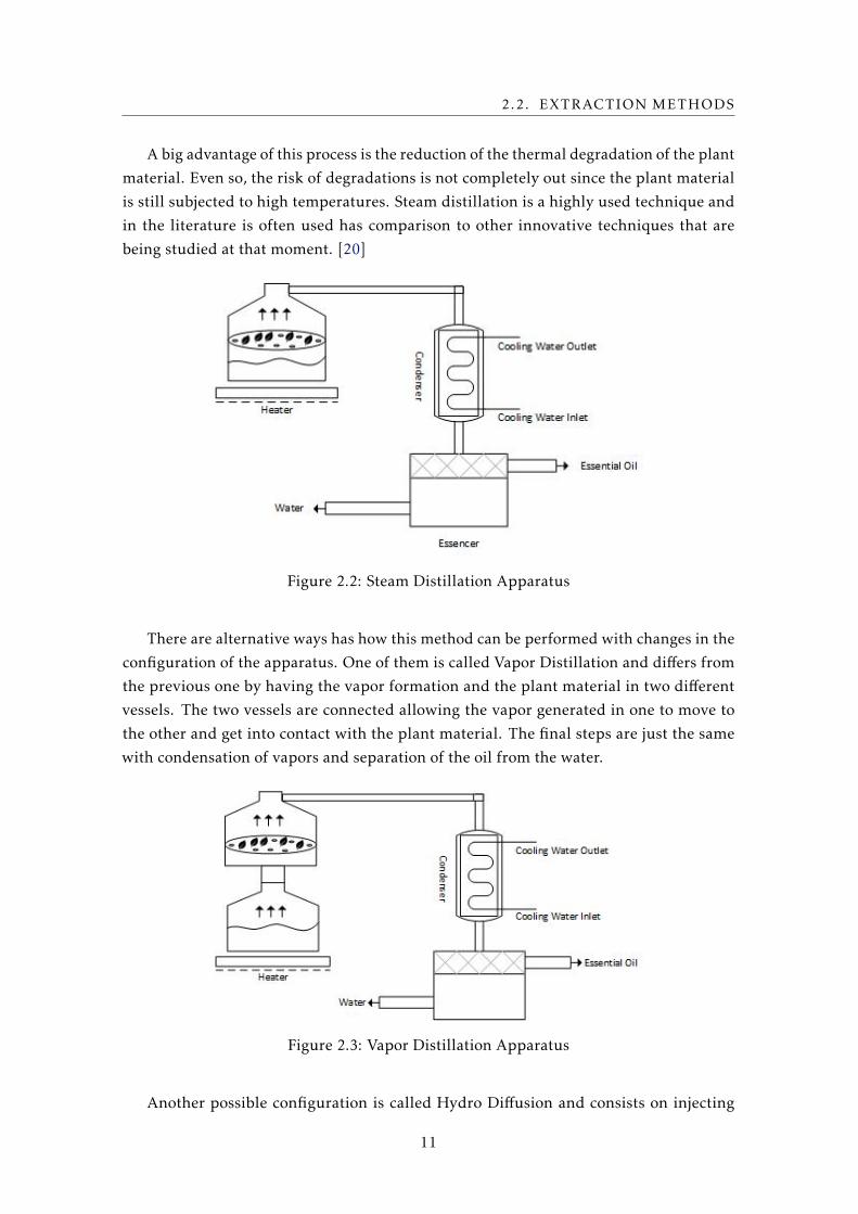
2.2.1.2 Steam Distillation
This technique consists in injecting water vapors through the plant matter which will
carry in the process volatile materials. The water vapor moves from the bottom up and
the boiling water is not in direct contact with the raw material which is suspended inside
the vessel in a grid or perforated plate. The same principles can be applied here since
water will be heated and turned into vapor, which will carry the volatile components.
They further suffer condensation and are separated by decantation. [12]
Steam Distillation is usually used in conditions of atmospheric pressure and tempera-
tures around 100oC.
Table 2.5: Literature on Steam Distillation.
Plant Temperature(oC) Pressure (bar) Reference
Ephedra sinica 100 1 [13]Origanum onites 100 1 [14]Rosmarinus officinalis. L 100 1 [15]Lavandula angustifolia 100 1 [16]Pogostemon cablin 100 1 [17]Mentha piperita 125 1 [18]Nepeta persica 100 1 [19]
10
2.2. EXTRACTION METHODS
A big advantage of this process is the reduction of the thermal degradation of the plant
material. Even so, the risk of degradations is not completely out since the plant material
is still subjected to high temperatures. Steam distillation is a highly used technique and
in the literature is often used has comparison to other innovative techniques that are
being studied at that moment. [20]
Figure 2.2: Steam Distillation Apparatus
There are alternative ways has how this method can be performed with changes in the
configuration of the apparatus. One of them is called Vapor Distillation and differs from
the previous one by having the vapor formation and the plant material in two different
vessels. The two vessels are connected allowing the vapor generated in one to move to
the other and get into contact with the plant material. The final steps are just the same
with condensation of vapors and separation of the oil from the water.
Figure 2.3: Vapor Distillation Apparatus
Another possible configuration is called Hydro Diffusion and consists on injecting
11

CHAPTER 2. THEORETICAL BACKGROUND
steam not from the bottom of the vessel but from the top making the steam move down-
ward. The vapor mixture with essential oils is directly condensed below the plant sup-
port through a perforated tray. This method can reduce the steam consumption and the
distillation tome, meanwhile, a better yield can be obtained in comparison with steam
distillation.
The conditions in which both of this two different configurations operate are the same
as in Steam Distillation with an atmospheric pressure and temperature close to water’s
boiling point.
2.2.1.3 Organic Solvent Extraction
This method consists on using organic solvents in order to separate two or more sub-
stances by dissolving the raw material and extracting the oil inside of it.
There are various types of possible apparatus in this technique being the most com-
mon the Sohxlet apparatus. This specific method uses a continuous circulation of organic
solvent in order to extract several compounds from the plant material of interest. The
solvent used is going to change from plant to plant being directly associated with the
compound supposed to be extracted. [20]
The continuous recirculation is possible since the physical state of the organic solvent
is changed first from liquid to vapor and later on again to liquid. The way the Soxhlet
extractor is design is so that after the organic solvent been boiled, the vapor goes through
a channel which leads to a condenser. In there, the organic solvent turns back into liquid
and fills the recipient where the plant material is located, extracting the components
from it. When the solvent reaches a certain level, it is sucked back to the beginning of the
process starting it all over again. To each time the solvent is recirculated back into the
heated vessel is called a cycle, being that denomination one of the most common ways to
describe how long the process is occurring. The Soxhlet extractor is then composed by
three main sections: A percolator which circulates the solvent, a thimble which retains
the solid to be laved and a siphon mechanism which periodically empties the thimble.
[21] [22]
Figure 2.4: Soxhlet Extractor.
12

2.2. EXTRACTION METHODS
The operating conditions of this method are also going to depend on the solvent used
for the extraction, performed at atmospheric pressure but with variable temperature since
the boiling point is different from solvent to solvent.
Table 2.6: Boiling Point of most common solvents.
Solvent Boiling Point (oC)
Acetone 56Dichloromethane 57,2
Hexane 68Ethanol 78,37
There are numerous examples of the use of this process in the literature, in fact, it’s
used in many cases as a standard process for comparison between tradition and new
developed extraction methods.
Table 2.7: Examples of solvent extraction in literature.
Plant Temperature(oC) Pressure (bar) Reference
Jasminum 78,4 1 [23]Origanum onites 68 1 [14]Eucalyptus loxophleba 90 1 [24]Agaricus bisporus L. 80 1 [25]Moringa oleifera 70 1 [26]Ricinus communis L. 68 1 [27]
One of the main advantages of this method is that needs no control over it, meaning
that the process can go through successive cycles without needing any outside action.
Usually the extraction is over by controlling the color in the heated vessel, to see if it has
high amount of the compound of interest.
2.2.1.4 Cold Pressing
Cold Pressing is a method which is based on machine squeezing the raw material at room
temperature for the release of essential oils, which are washed in cold running water.
The oil is then separated from the water by centrifugation or by simple decantation.
Even though the end result and theory involved are the same, there are several types
of machines with different configurations, using from plates to screws to perform the
extraction. The oils originated from this method are mainly used in cooking applications,
like for example oils from olive and sunflower. Since the process itself is mechanic the
operating conditions are usually at normal pressure and temperature, which makes the
raw material not has exposed to big sources of heat, making possible less degradation of
the oil to occur. Other big example of this method is the extraction from Citrus peel since
not only there’s a large quantity of oil in this material but it has also a very low cost to
grow and harvest the raw materials. [28]
13

CHAPTER 2. THEORETICAL BACKGROUND
Figure 2.5: Cold Pressing apparatus.
Even though is not has popular has the other methods, cold pressing is also referred
in literature as a comparison method.
Table 2.8: Examples of cold pressing extraction in literature.
Plant Temperature(oC) Pressure (bar) Reference
Citrus fruits Normal Temperature 1 [11]Camelina sativa Normal Temperature 1 [29]Rheum rhaponticum L. Normal Temperature 1 [30]Juglans regia L. var. Franquette 25/50/70 1 [31]Canola seeds Normal Temperature 100 [32]Vitis vinífera L. Normal Temperature 1 [33]
As it was mentioned before, one of main advantages of this type of extraction rests
on the fact that it doesn’t use high temperatures avoiding oil degradation. Another major
advantage of this method is the fact that it doesn’t use organic solvents, turning this
process not only much safer, but also simpler since no solvent separation processes are
needed prior the extraction.
Through this method is also possible to retain bioactive compounds such as essential
fatty acids, phenolics, flavonoids and tocopherols in the oils. In some cases, after the
centrifugation part of the process some other products besides the oil might be used to
other applications like proteins, minerals, and other substances.
14

2.2. EXTRACTION METHODS
2.2.2 Green Extraction with Innovative Methods
In modern industrial production the words eco-friendly, sustainability, high efficiency
and quality become more and more common. By applying the concepts of green extrac-
tion in creating processes which would allow reducing operation units, energy consump-
tion, CO2 emissions, among other factors new methods were developed has alternatives
to the most traditional ones. The focus of this new processes is not just to improve the
One of main disadvantages of conventional techniques is the fact that essential oils
components are highly sensitive to heat and can easily suffer chemical alterations (isomer-
ization, oxidation) due to the high applied temperatures.
2.2.2.1 Subcritical Extraction
Subcritical Fluid Extraction is a method in which the solvent substance is operated in con-
ditions close of critical pressure (Pc) and temperature (Tc). In simple terms, the subcritical
conditions are achieved by changing these parameters along the critical point. From the
literature is possible to see that the most common fluids used in this type of processes are
water and carbon dioxide (CO2).
Table 2.9: Literature examples of subcritical extraction.
Plant Solvent Temperature(oC) Pressure (bar) Reference
Contaminated Soil Water 250 - 300 50 [34]Coriandrum sativum L. Water 100 - 175 20 [35]Curcuma longa L. Water 120 - 160 10 [36]Red Paprika CO2 6 56 [37]Coriandrum sativum L. Water 350 200 [38]Thymus mastichina Water 100 - 175 20 - 200 [39]
• Subcritical Water Extraction (SWE)
Subcritical Water Extraction it’s a technique which operates at temperatures between
100 and 374oC and pressure high enough to maintain the liquid state. Usually the tem-
perature used in this type of processes is 200oC. It can be performed in batch or continue
systems, being the last the most common.
One possible apparatus configuration for this type of process is for the case of subcrit-
ical extraction using water as solvent. This system uses tanks, pumps, extraction vessels,
oven for the heating of the extraction vessel, heat exchangers for cooling of extract and
a sample collection system. The pump is essentially employed for pumping the water
(and extract) through the system. In some other cases, another pump can be employed
for flushing the tubing’s. Also, one extra tank can be employed to contain an organic
solvent which would act as a co-solvent (modifier), being necessary to use another pump
in order to introduce it into the system. A pressure restrictor is needed to maintain the
appropriate pressure in the equipment. [20]
15

CHAPTER 2. THEORETICAL BACKGROUND
Figure 2.6: Subcritical Water Extraction apparatus example has described above.
The unique properties of water are namely its disproportionately high boiling point
for its mass, a high dielectric constant and high polarity. As the temperature rises, there is
a systematic decrease in permittivity, an increase in the diffusion rate and a decrease in the
viscosity and surface tension. This way, more polar target materials with high solubility in
water at ambient conditions are extracted more efficiently at lower temperatures, whereas
moderately polar and non-polar targets require a less polar medium induced by elevated
temperature. The most important parameters in this type of process are then temperature,
particle size and flow rate.
This method also functions has a powerful alternative to more traditional extraction
methods since it uses low working temperatures and enables a rapid extraction. Other
positive aspects in using this technique are its simplicity, low cost, and favorable environ-
mental impact. Also when compared to the various traditional methods, Subcritical Water
Extraction presents several advantages like shorter extraction times, higher quality of the
extract, lower costs of the extracting agent, an environmentally compatible technique and
low solvent consumption.
In the literature comparisons can be found between supercritical CO2 and SWE, con-
cluding that even though the extraction conditions are softer and less expensive to run
that supercritical CO2 the last still becomes cheaper to implement on an industrial level,
since SWE requires specific equipment.
• Extraction with Subcritical CO2
The subcritical state of carbon dioxide (CO2) is obtained when the temperature is
between 31oC and 55oC and pressure between 0.5 MPa and 7.4 MPa. Under these condi-
tions the CO2 behaves as a non-polar solvent. The apparatus for this type of process is
similar to the configuration presented on the Subcritical Water Extraction process, chang-
ing only on the extracting solvent. This type of process can also incorporate various types
of modifiers in order to improve the extraction results.
16
2.2. EXTRACTION METHODS
This method avoids the degradations observed in the steam distillation or entrainment
by vapor due to the high temperatures and the presence of water. According to the
literature, extracts obtained by this technique present flavors very similar to those of
fresh vegetable raw materials. Also, when compared to SWE its shown to have a superior
quality of extract. [20]
2.2.2.2 Ultrasound Assisted Extraction
This method uses ultrasounds in order to allow the intensification of the extraction pro-
cess from the plant raw material when used in combination with other techniques like
hydrodistillation and solvent extraction. Ultrasounds are essentially sound waves with
frequencies higher than the upper audible limit of the human hearing. [40]
The plant raw material is immersed in water or solvent and at the same time it is
subjected to the action of the ultrasound. This technique was developed especially for
the extraction of certain molecules of therapeutic interest even though nowadays it its
used for large number of other applications.
Commonly, the used ultrasonic waves have a frequency of 20 kHz – 1MH. This waves
will induce mechanical vibrations on the walls and membranes of the plants allowing a
faster extraction. A very important parameter in this type of processes is the size of the
particles, or in other words, the milling degree of the plant material. The smallest the
size the more particles will be subjected to the action of the ultrasound waves. [20]
In terms of equipment necessary, it’s very simple since it consists in only adding an
ultrasound generator to an already existing extraction process. This makes its implemen-
tation not only very simple but also very inexpensive.
When compared with the more traditional methods, it presents advantages such as
improving extraction efficiency and rate, a reduction in the extraction temperature, and
increasing the selection range of solvents that can be used. Finally, other advantages of
this method consist in the properties of ultrasound which can be an intensification of the
mass transfer, cell disruption, improvement of solvent penetration and capillary effect.
Ultrasound Assisted Extraction has been growing in terms of applications since it’s a
simple way to improve already establish extraction methods.
Table 2.10: Literature Examples of Ultrasound Assisted Extraction.
Plant Assisted Process Reference
Lavandula intermedia Steam Distillation [8]Artemisia annua L. Hot Maceration [41]Olea europaea Maceration [42]Artocarpus heterophyllus Solvent Extraction [43]Limonium sinuatum Solvent Extraction [44]Allium tuberosum Solvent Extraction [45]
17

CHAPTER 2. THEORETICAL BACKGROUND
2.2.2.3 Microwave Assisted Extraction
Microwave Assisted Extraction also becomes an innovative technique by allowing to im-
prove methods already existent. The use of this technique evolved with the development
of the green extraction method concept and the need for new energy saving extraction
methods.
Microwaves are electromagnetic based waves with a frequency between 300 MHz and
30 GHz and a wavelength between 1 cm and 1 m. The commonly used frequency is 2450
MHz which corresponds to wavelength of 12,2 cm. [20]
In recent times, this process has developed several variants such as microwave as-
sisted hydrodistillation, solvent free microwave extraction, microwave -accelerated steam
distillation, microwave steam distillation, microwave hydrodiffusion and gravity and
portable microwave assisted extraction. It consists on one of the most promising tech-
niques, presenting advantages such has high reproducibility in shorter times, simplified
manipulation, reduced solvent consumption and lower energy output.
Table 2.11: Literature examples on Microwave Assisted Extraction.
Plant Assisted Process Reference
Citrus fruits Distillation [11]Soil Solvent Extraction [46]Lavandula angustifolia Steam Distillation [16]Aromatic herbs Hydro-distillation [47]Thymus vulgaris L. Hydro-distillation [48]Curcuma longa Solvent Extraction [49]
From all the variants there were some worth specifying:
• Solvent free microwave extraction (SFME)
This variant is based on the combination of microwave heating energy and dry distil-
lation, in order to achieve at atmospheric pressure, the extraction of a fresh plant material
without the need of adding any water or organic solvents.
Figure 2.7: SFME apparatus.
18

2.2. EXTRACTION METHODS
• Microwave hydrodiffusion and gravity (MHG)
This method consists in placing the plant material in a reversed microwave reactor
without any added water or solvent. It combines microwave heating of a reversed alembic
with the earth gravity at atmospheric pressure.
When the water inside the plant is heated by the microwaves, causes the rupture
of the material allowing to obtain the extracts. Under gravity, these extracts fall to the
bottom out of the microwave reactor and in direction to the cooling system.
Figure 2.8: MHG apparatus.
From the literature is possible to conclude that this method not is power saving, but
reduces extraction time and environmental impact.
• Microwave steam distillation (MSD)
In this case the same principles regarding the effect of the microwaves on the plant
material apply. It results from a modification of the traditional steam distillation method
in which by action of the microwaves the plant material will release its components in a
faster way being then carried by the steam in a condenser so the extract can be collected.
Figure 2.9: MSD apparatus.
19

CHAPTER 2. THEORETICAL BACKGROUND
In comparison to the traditional methods it was proven to reduce the extraction time
and better sensory properties by allowing the high production of fresh oil without causing
significant changes in its composition.
• Microwave steam diffusion (MSDf)
It is based on the same principles as for the Microwave Steam Distillation (MSD)
except that vapors flow through the plant material down.
Figure 2.10: MSDf apparatus.
Microwave steam diffusion is a green cleaner, environmentally friendly and an eco-
nomic procedure.
2.2.2.4 Supercritical Fluid Extraction
Supercritical Fluid Extraction has emerged as an attractive separation technique for the
food and pharmaceutical industries due to a growing demand for natural processes that
do not introduce any residual organic chemicals. It uses fluids in well-defined conditions
of pressure and temperature and when those conditions are reached, the fluids manifest
very interesting properties like high diffusivity, low viscosity, and a density close to that
of liquids. [20]
Supercritical fluid extraction can be accomplished using a static, dynamic, or coupled
static/dynamic mode. In static extraction, a fixed amount of supercritical fluid interacts
with the plant material. The extraction vessel containing the plant material is pressurized
with the chosen fluid at a certain temperature. The high diffusivity of the supercritical
fluid allows it to go through the plant material removing the components of interest.
After the extraction is completed, a valve is open allowing the extract to be removed
20

2.2. EXTRACTION METHODS
by decompression into a trap. Usually, a static extraction is followed by some time of
dynamic extraction in order to improve the extraction efficiency. In some cases, the
supercritical fluid can be recovered in order to introduce it into the process again.
Figure 2.11: Static Supercritical Extraction apparatus.
When it comes to dynamic extraction, this uses fresh supercritical fluid which is
continuously passed through the plant material. A big concern of this type of processes
is that impurities in supercritical fluids become a concern when using large amounts of
fluid during an extraction. Other problems of this type of extraction are the fact that a
larger amount of supercritical fluid will eventually extract non wanted components and
also cause motion of the plant material which could cause clogged problems. In spite of
these problems, dynamic extraction is the favored strategy for at least 90% of all reported
applications of supercritical fluid extraction.
Figure 2.12: Dynamic Supercritical Extraction apparatus.
A combination of an initial static period followed by a dynamic one is gaining popu-
larity, especially for situations where solvated analyte must diffuse to the matrix surface
to be extracted. The extraction starts in a static mode with no net flow through the system.
When the extraction has proceeded for a given amount of time, the system is put into a
dynamic mode.
Supercritical Fluid Extraction can be influence by several parameters:
21

CHAPTER 2. THEORETICAL BACKGROUND
• Particle size and shape;
• Surface area and porosity;
• Moisture content;
• Changes in morphology;
• Sample size.
Carbon dioxide (CO2) is generally the most widely used solvent for extraction because
of its numerous advantages. The most important ones are having a critical point easy
to reach (a critical pressure of 73,9 bar and a critical temperature of 31,2oC), being un-
aggressive for thermolabile molecules of the plant essence, being chemically inert and
non-toxic, non-flammable, available in high purity at relatively low cost, and allows easy
elimination of its traces from the obtained extract by simple depression.
Table 2.12: Literature examples on Supercritical Extraction.
Plant Solvent Process type Reference
Eucalyptus loxophleba CO2 Dynamic [24]Syzygium aromaticum CO2 Stationary [50]Leptocarpha rivularis CO2 Stationary/Dynamic [51]Anethum sowa CO2 Stationary [9]Myristica fragrans CO2 Dynamic [52]Carum copticum CO2 Static/Dynamic [10]Mentha pulegium L. CO2 Static/Dynamic [53]Foeniculum vulgare CO2 Static [54]Marchantia convoluta CO2 Static/Dynamic [55]Lippia alba CO2 Dynamic [56]Rosmarinus officinalis CO2 Static [57]Rose geranium CO2 Dynamic [58]Matricaria chamomilla CO2 Static [59]Cuminum cyminum L. CO2 Dynamic [60]
Essentially this is a process which is based on the use and recycling of fluid in repeated
steps of compression and depression. The use of this technique in extraction has grown
in the most recent years, being one of biggest obstacles to its development the high cost
in equipment, installations and maintenance operations.
Also, extracts from this technique presented a higher quality, possessing better func-
tional and biological activities in comparison with extracts produced by some more tradi-
tional techniques. Studies also showed a better antibacterial and antifungal properties in
supercritical products.
The major limitations of this process as mentioned before have to do with the cost
associated, which increases as the pressure conditions considered also become higher.
Also already mentioned, CO2 is the main solvent used in this type of processes, which
22

2.3. SUPERCRITICAL FLUIDS
also brings limitations to the process since its non-polarity limits the dissolving power
of this solvent. This fact makes so that CO2 can’t be used on it’s on in a wide range of
processes, especially in the extraction of most polar compounds. To solve this problem,
organic solvents are added to the process in order to improve the extraction capabilities
of the solvent to those compounds of interest.
The organic solvents are usually called modifiers and the most common used in this
type of processes are ethanol, methanol, hexane, water, dichloromethane, chloroform,
formic acid, among others. They have influence in a large number of properties like
increase and decrease of polarity, chirality, and the ability to further complex metal-
organic compounds. The use of modifiers may create the idea that the process is not
as environmental friendly has previously thought but the reality is that these organic
solvents are used in very small amounts and when the yields are compared, what comes
across in most cases is an improvement of the extraction process which makes its use
worth it.
Compared with traditional methods, supercritical extraction presents several advan-
tages like allowing a faster extraction process, being suitable for extraction and purifica-
tion of compounds having low volatility present in solid or liquid, minimizes the risk of
thermal degradation, and becomes a versatile and efficient process with multiple config-
urations. The limitations of this type of process are an inaccurate modeling, the impos-
sibility to scale, its consistency and reproducibility may vary in continuous production,
and as it was mentioned before it becomes an expensive process to assemble because of
the special high pressure equipment necessary.
2.3 Supercritical Fluids
It is now 186 years since Baron Charles Cagniard de la Tour discovered that, above a
certain temperature, single substances do not condense or evaporate, but exist only as
fluids. He noted visually that the gas-liquid boundary disappeared when the temperature
of certain materials was increased by heating each of them in a closed glass container.
A fluid is characterized has a substance that continually deforms under an applied
shear stress. They are a subset of the phases of matter and include liquids, gases, plasmas
and also plastic solids. In the following years, the concept of “critical point” was studied
and characterized by the parameters of critical pressure (Pc) and critical temperature (TC).
Studies were then carried around this area, above and below, in order to see the behavior
of this fluids by changing the conditions of pressure and temperature. [61]
A critical point of a substance is characterized by the point which represents the end
of the phase equilibrium curve. As it was mentioned before, this point is achieved when
specific conditions of temperature and pressure are reached, which are designated as
critical temperature (Tc) and critical pressure (Pc). The value of this point change from
substance to substance and causes changes in its physical properties.
23

CHAPTER 2. THEORETICAL BACKGROUND
Figure 2.13: Illustration of the critical point.
Table 2.13: Critical Conditions for most common solvents.
Solvent Critical Temperature Critical Pressure Critical Density(oC) (atm) (g/cm3)
Carbon Dioxide 30,95 72,8 0,469Water 373,95 217,8 0,322
Methane -82,75 45,4 0,162Ethane 32,15 48,1 0,203
Propane 96,65 41,9 0,217Ethylene 9,25 49,7 0,215
Propylene 91,75 45,4 0,232Methanol 239,45 79,8 0,272Ethanol 240,75 60,6 0,276Acetone 234,95 46,4 0,278
Nitrous Oxide 33,42 72,5 0,452
There are two main fluid states around the critical point, the subcritical and the
supercritical state. The subcritical state is reached when a substance is subjected to
a pressure higher than the critical pressure (Pc) and a temperature bellow the critical
temperature (Tc), or vice versa. In this state, fluids present a wide range of properties
like low viscosity, density close to that of liquids, and the diffusivity between that of
a gas and a liquid. Subcritical fluids are not as studied has supercritical ones and the
level of applications is not as big. On the other hand, in most cases they become much
more easy to achieve the conditions necessary for this state, allowing a certain variability
between pressure and temperature. In some cases, like extraction what happens is that
the temperature can be low so no thermal degradation occurs and the pressure can be
risen above the critical point, achieving the subcritical state anyway.
Supercritical fluids are essentially any substance at a temperature and pressure above
its critical point, where distinct liquid and gas phases do not exist. It can effuse through
24

2.3. SUPERCRITICAL FLUIDS
solids like a gas, and dissolve materials like a liquid. In the supercritical region the fluid
presents specific properties like an intermediate behavior between that of a liquid and of
a gas, high diffusivity and low viscosity.
Figure 2.14: Representation of the various states until achieving a supercritical fluid.
From the image above it’s possible to see that in a first stage there’s a clear separation
between gas and liquid phases. With the increase in pressure and temperature it’s possible
to see that the separation gradually vanishes becoming more and more like a one phase
system. [62]
As it was previously said, the supercritical state can be achieved when a specific set
of conditions are surpassed (critical pressure (Pc) and critical temperature(Tc)). Different
compounds possess different values of critical pressure and temperature, so even if a
substance can be putted in a supercritical state it might not be worth to introduce it into
a process.
It’s clearly possible to see that from all the compounds presented above that CO2 is
the one with the easiest conditions to reach the critical point, being that one of the reasons
for it to be the most common supercritical solvent. Other advantages of supercritical CO2
are:
• Safe and environmentally friendly;
• Recyclable, in a sense that after its use on a certain process in can be recapture and
used again in the process;
• Inexpensive and easily available;
• No residue is left after its use;
25

CHAPTER 2. THEORETICAL BACKGROUND
• On contrary to other popular solvents it has zero surface tension. This factor can be
compared with other existent solvents in the table presented below.
Table 2.14: Viscosity, Surface Tension and Density comparison between solvents.
Solvent Viscosity Surface Tension(cP) (dyne/cm)
Liquid Carbon Dioxide 0,08 1,5Supercritical Carbon Dioxide 0,03 0
Methanol 0,54 22,11,1,1-Trichloroethane 0,81 25,2
Water 1,0 72,0Isopropyl Alcohol 2,4 21,8
Supercritical fluids can occur on the nature in cases like hydrothermal circulation
and planetary atmospheres. In the bottom of the ocean certain areas possess heat spots
which in combination with the pressure in the bottom of the ocean might create these
type fluids. In the case of planetary atmospheres such fluids can be found in planets
like Venus, Jupiter, and Saturn. This type of planets, are mainly composed by gases like
carbon dioxide, hydrogen, helium and nitrogen.
Due to its many advantages, supercritical CO2 is used in a large range of applications.
Supercritical fluids in general first started only being used on analytical chemistry, and
not much support was given to its application. A significant change happened when a
patent was released reporting the decaffeination of green coffee using supercritical CO2.
From that moment on a significant development on the use of supercritical fluids started,
especially when referring to supercritical fluid extraction (SFE).
The supercritical fluid extraction can be applied in the extraction of hops, choles-
terol from butter, perfumes and flavors from natural products, and unsaturated fatty
acids from fish oils. Other more specific applications can be impregnation and in situ
deposition of chemicals, cleaning of electronic parts, nucleation and particle size reg-
ulation, chemical reaction and synthesis of organic chemicals and remediation of soil.
There are so many applications that supercritical fluid technology has become an inter-
disciplinary field, utilized by chemical engineers, chemists, food scientists, materials
scientists, agronomists, and researchers in biotechnology and environmental control.
In the last ten years, the range of supercritical fluids has expanded from commod-
ity chemicals and synthetic fuels toward more complex, highly specialized, and more
valuable substances. In addition to applying the technology for the purpose of new prod-
uct isolation and purification, considerable effort has been devoted to gaining a better
fundamental understanding of molecular structure, phase behavior, solvation processes
between solute and fluid phase, and transport properties of supercritical fluids.
The disadvantages of supercritical fluids are that high pressures and sometimes tem-
peratures are involved, and, in the case of water, there are corrosion problems. As the
26

2.4. ANALYTICAL METHODS
technology to overcome them is available, these disadvantages become cost and conve-
nience factors to weight against potential advantages.
Table 2.15: Main applications for supercritical fluids
Pharmaceuticals: Foods:Extraction of biologically active Ingredients; Flavor Extracting and concentrationFermentation broth extraction; Extraction of flagranceProtein purification. Processing essential oils
Flavor and fragrance infusionNutraceuticals: Polymers:Vitamin Extraction; Renewal of monomers an oligomers;Concentration of active ingredients; Infusion of components;Anti-oxidant extraction. Removal of binder from powered metals.Cleaning: Reaction Chemistry:Precision machined components; Reactions and organic product synthesis;Silicon wafers; Hydrogenation Reaction;Medical Implants and electronic components. Polymerization reactions and synthesis.
2.4 Analytical Methods
The analytical methods are an essential part of any project of this nature. Even though
the aim of the work is focus in extraction and not in analytical methods, these are the
ones who allow us to understand what was obtained and in certain cases in how much
was actually extracted. When it comes to the analyzes of plant materials there are several
methods found in the literature which are constantly used. Some of the most referenced
are Gas Chromatography copulated with a Mass Spectrometer (GC/MS), High Perfor-
mance Liquid Chromatography (HPLC), Thin-layer chromatography (TLC) or simply Gas
Chromatography (GC).
Table 2.16: Literature analytical methods examples.
Plant Analytical Method Reference
Asarum species GC [63]Lavandula species GC, GC/MS [64]Berberis tinctoria Lesch. GC/MS [65]Berberis vulgaris L. HPLC [66]Berberis croatica/vulgaris HPLC [67]Eucalyptus loxophleba GC/MS [24]Anethum sowa GC, TLC [9]Carum copticum GC, GC/MS [10]Mentha pulegium L. GC, GC/MS [53]Foeniculum vulgare GC [54]Marchantia convoluta GC/MS [55]Lippia alba TLC, GC [56]
27

CHAPTER 2. THEORETICAL BACKGROUND
Rosmarinus officinalis GC, TLC [57]Matricaria chamomilla HPLC [59]Ilex paraguariensis GC/MS [68]Ocotea odorifera GC/MS [69]Origanum onites GC/MS [14]Rosmarinus officinalis. L GC/MS [15]Matricaria chamomilla GC/MS, HPLC [70]Pogostemon cablin GC/MS [17]Ocimum basilicum L. GC, GC/MS [71]Mentha piperita GC/MS [18]Nepeta cataria L. GC, GC/MS [19]Artemisia annua GC/MS [72]
The technique used depends from the objectives of the experiments, essentially of
what is intended from the sample. For example, in the case of plant extraction, most
authors choose to use HPLC or GC/MS since these techniques allow an analytical and
quantitative analyzes. Other methods like GC on the other hand, only allow a simpler
representation which ends up not being sufficient to prove that one or more compounds
are present in the analyzed sample.
• Gas Chromatography (GC)
This technique allows to separate all of the components in a sample and provides a
representative spectral output. The sample is injected into the injection port while the de-
vice vaporizes it for later separate and analyze the various components. The temperature
of the injection port must be high enough to vaporize a liquid specimen instantaneously.
[73]
Figure 2.15: Gas Chromatography (GC) apparatus.
The time between injection and elution is called the “retention time”. The size of the
peaks is proportional to the quantity of the corresponding compound in the substance
analyzed. The retention time for a compound is not fixed as many factors can influence
it even if the same GC and column are used. These factors include the gas flow rate,
temperature differences in the oven and column, column degradation, and column length.
These factors can make it difficult to compare retention times since that even if you use
28

2.4. ANALYTICAL METHODS
the same GC just a few days apart, there could be a small difference in the retention time
of a compound.
Figure 2.16: Example of GC output.
There are several types of detectors used in Gas Chromatography,
• Argon Ionization Detector;
• Flame Ionization Detector;
• Flame Emission Detector;
• Cross Section Detector;
• Thermal Conductivity Detector;
• Electron Capture Detector.
The type of detector used will depend on the properties of the compounds of interest
since that the wrong choice could cause their degradation influencing the end results.
• GC/MS
This method represents a combination of the GC method explained above with Mass
Spectrometry (MS). This technique allows to identify substances by electrically charging
the specimen molecules and accelerating them through a magnetic field. This allows to
break the molecules into charged fragments and detecting the different charges. [74]
A spectral plot displays the mass of each fragment and through the small masses
presented is possible to reach the value of the “parental” mass. This value when compared
with the literature allows the identification of a compound.
29
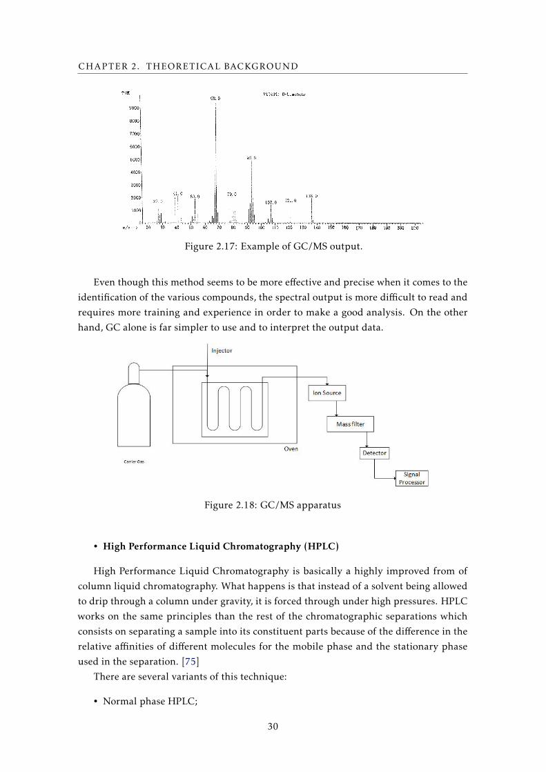
CHAPTER 2. THEORETICAL BACKGROUND
Figure 2.17: Example of GC/MS output.
Even though this method seems to be more effective and precise when it comes to the
identification of the various compounds, the spectral output is more difficult to read and
requires more training and experience in order to make a good analysis. On the other
hand, GC alone is far simpler to use and to interpret the output data.
Figure 2.18: GC/MS apparatus
• High Performance Liquid Chromatography (HPLC)
High Performance Liquid Chromatography is basically a highly improved from of
column liquid chromatography. What happens is that instead of a solvent being allowed
to drip through a column under gravity, it is forced through under high pressures. HPLC
works on the same principles than the rest of the chromatographic separations which
consists on separating a sample into its constituent parts because of the difference in the
relative affinities of different molecules for the mobile phase and the stationary phase
used in the separation. [75]
There are several variants of this technique:
• Normal phase HPLC;
30

2.4. ANALYTICAL METHODS
• Reverse phase HPLC;
• Size exclusion HPLC;
• Ion exchange HPLC;
HPLC results can be influenced by parameters such as the Internal diameter of the
column, particle size, pore size, pump pressure, and by the type of detectors used.
There are some different types of detectors such as UV-spectroscopy, fluorescence, mass-
spectrometric and electrochemical detectors.
Figure 2.19: Example of an HPLC apparatus
• Differential Scanning Calorimetry (DSC)
Differential Scanning Calorimetry (DSC) consists on a technique in which the differ-
ence in the amount of heat required to increase the temperature of a sample and reference
is measured as a function of temperature. Both the sample and reference are maintained
at nearly the same temperature throughout the experiment. Two types of DSC:
• Power compensated DSC, in which the power supply is kept constant.
• Heat flux DSC, which keeps constant the heat flux.
A basic principle underlying this technique is that when the sample undergoes a
physical transformation such as phase transitions, more or less heat will need to flow to
it then the reference to maintain both the same temperature. Whether less or more heat
must flow to the sample depends on whether the process is exothermic or endothermic.
If a process is exothermic then the system will need to transfer less heat to match the
31

CHAPTER 2. THEORETICAL BACKGROUND
reference temperature, while the opposite happens if the process is endothermic since it’s
removing heat from the system so it takes more heat to increase the temperature. [76]
As it was mentioned before there are several techniques used for analyses of extracts
but only this were quickly described since they will serve as based for the future work.
Figure 2.20: Example of an DSC apparatus
32

Chapter
3Safrole - Extraction and Reaction
This chapter is dedicated to show the work developed on the substance safroleand the research performed on its extraction and epoxidation reaction.
3.1 Sassafras
3.1.1 Sassafras Plant
Sassafras is a genus in the family Lauraceae, native from eastern North America and
eastern Asia. Its trees grow from 9 to 35 meters tall and usually present an orange-brown
or yellow bark. The Sassafras genus contains three surviving and one extinct species,
which are Sassafras albidum, Sassafras tzumu, Sassafras randaiense, and Sassafras hesperiarespectively.
Native Americans have used Sassafras for centuries by rubbing the leaves directly
into a wound, and using different parts of the plant for many medicinal purposes such as
treating acne, urinary disorders, and high fevers. Sassafras has also been applied to insect
bites and stings to relieve symptoms, and is also known to be used as a sudorific agent in
eye inflammation treatment, rheumatism, gout, swelling, and cutaneous eruptions. Be-
fore the twentieth century, Sassafras enjoyed a great reputation in the medical literature
and became valued for its power to improve the flavor of other medicines. It also repre-
sents a food source for many types of animals. Leaves, bark, stems, and fruits are often
eaten by birds and mammals like porcupines, groundhogs, marsh rabbits, and American
black bears in small quantities. When it comes to humans this plants are mostly used for
culinary, medicinal, and aromatic purposes. [77]
The main extract in this type of plants is the essential oil with the amount extracted
depending on the section of the plant considered, and varying from plant to plant. In
the case of Sassafras albidum the highest amount of oil that can be obtain comes from the
33

CHAPTER 3. SAFROLE - EXTRACTION AND REACTION
root bark and corresponds to about 10%. Its other constituents are camphorous matter,
resins, wax (decomposition product of Sassafrid), tannic acid, gum, albumen (Egg White),
starch, lignin and salts. [78]
Figure 3.1: Sassafras albidum tree.
Has it been mentioned before the Sassafras family is composed by four main types
of plants. Of this four, Sassafras hesperia is extinct and the plants of interest in terms
of safrole content are Sassafras albidum and Sassafras tzumu. Sassafras albidum is native
to eastern North America and usually grows at altitudes up to 1500 meters, achieving a
height of 15 to 20 meters. The leaves are alternate, green to yellow green and its fruit is
characteristically dark-blue. From medical proposes to culinary applications the range
of uses of this plant is enormous, being now a day extremely related to drug production
since its safrole content is around 88%.
Table 3.1: Sassafras albidum oil composition.
Compound CompositionSafrole 82,8% - 88,8%
Camphor 1,2% - 6,8%Methyl Eugenol 1,4% - 2,3%
Eucalyptol (1,8-cineole) 1,1%
Sassafras tzumu is native to China and grows at altitudes from 100 to 1900 meters
reaching heights up to 35 meters. Its wood is mainly used for shipbuilding and furniture
making because of its durability. Essential oils can be extracted from barks, roots, or fruit
having a safrole content of 97%.
34

3.1. SASSAFRAS
Table 3.2: Examples of other plants with high content in Safrole.
Plant Plant Part Safrole ContentCinnamomum burmanni Leaf 97 – 99%Cinnamomum camphora Root bark 50 – 80%
Cinnamomum micranthum Wood 95%Cinnamomum parthenoxylon Wood 80%
Cinnamomum paucifolium Leaf 68 – 90%Cinnamomum petrophilum Leaf 97%
Curcuma amada Rhizome 9.3%Octea cymbarum Wood 84 – 93%Piper callosum Leaf 70%
Piper hispidinervium Leaf 81 – 88%
3.1.2 Sassafras Oil
Sassafras oil is a yellow liquid which results of applying extraction methods on Sassafrasgenus plants. This oil can be extracted using multiple processes like Steam distillation,
Organic Solvent extraction, Supercritical Fluid Extraction, among others. This oil is
characterized by being mainly composed by safrole, however, its content and form the
other compounds which also make part of the oils composition, end up variating with
the type of plant from where they’re extracted from. [79]
The oil has been applied through the history in multiple areas like food and medicine.
It was believed to hold the cure from problems like hangovers to serious conditions like
syphilis. The Europeans first discover the properties of this oils when arrived to America,
and didn’t waste time in starting ship it to Europe. Since that, Sassafras oil has been used
in a huge variety of foods, medicines, and other products.
Figure 3.2: Sassafras oil.
One example of this applications is root beer, being extremely popular in places like
the United States of America. This component was later prohibited due to its high content
35

CHAPTER 3. SAFROLE - EXTRACTION AND REACTION
in safrole which was proven to have carcinogenic properties. The recently discovered
properties of the oil cause many applications to be dropt or in research to find substitutes
with less health impact.
Due to this, the market of this oil is today very reduced and highly controlled espe-
cially because of safrole, making its isolation the main application of the oil.
Figure 3.3: Root beer, one of the past main applications for Sassafras oil.
3.2 Safrole
Safrole is a naturally occurring substance which exists at room temperature as a colorless
or pale yellow liquid with an odor of sassafras. This compound is highly soluble in alcohol,
miscible with chloroform and ether, and practically insoluble in water. [79]
Table 3.3: Safrole Properties.
Properties Data
Molecular weight 162,2 g/molDensity 1,1 g/cm3 at 20◦CMelting point 11,2◦CBoiling point 234,5◦CVapor pressure 0,0618 mmHg at 25◦C
Safrole has been used as a flavoring agent in drugs and in the manufacture of he-
liotropin, perfumes, soaps, and piperonyl butoxide (a compound used in insecticides to
enhance the its properties).
It is also a substance highly controlled since not only the raw material is used for
the illicit production of the drug 3,4 – methylenedioxymethamphetamine (MDMA, or
ecstasy) but also it was proven to be highly carcinogenic. For that reason, besides the many
applications, any addition of safrole or oil of Sassafras to food is extremely forbidden.
36

3.2. SAFROLE
Figure 3.4: Main safrole application today: Ecstasy
Safrole is on the lists for controlled substances as a drug precursor by organizations
like the European Union, The United Nations, FDA, among others. The common daily
intake of this substance, according to the literature, is around 0,3 mg. Even with strict
control, safrole is naturally present in natural products like Sassafras tree and in edible
spices like cinnamon, nutmeg, ginger, and black and white pepper.
3.2.1 Safrole Oxide
In more recent years, the epoxidation reaction of safrole has been studied in order to
obtain has product safrole oxide. This compound doesn’t exist naturally and can only be
obtain by the reaction of safrole. Safrole oxide has a chemical formula of C10H10O3 and
at normal temperature can be found as a solid.
Figure 3.5: Safrole Oxide Structure
By its structure it’s possible to observe that it differs from safrole by possessing one
more oxygen (O) atom. The double bound at the end of the safrole molecule allows for
that extra Oxygen to bind forming a new molecule with different properties associated to
it.
37

CHAPTER 3. SAFROLE - EXTRACTION AND REACTION
Table 3.4: Safrole Oxide Properties.
Properties Data
Molecular Weight 178,2 g/molMelting point 61,23 ◦CBoiling point 265,82 ◦CVapor pressure 0,00911 mmHg at 25◦C
The traditional way of obtaining safrole oxide by epoxidation of safrole is done by
reacting it with m-chloroperbenzoic acid (mCPBA).
Figure 3.6: Epoxidation of safrole using MCPBA has an oxidizing agent.
The compound m-chloroperbenzoic acid (mCPBA) is a peroxycarboxylic acid used
widely as an oxidant in organic synthesis and it’s preferred to other peroxy acids because
its relatively easy to handle. The main applications for this compound can be found in
processes where oxidation of ketones, sulfides, amines, and also alkenes occurs. Even
then it’s relatively stable still presents some risks like causing fire upon contact with
flammable materials.
Figure 3.7: mCPBA Structure.
The recent interest in safrole oxide has to do with its anti-angiogenesis and apoptosis-
inducing activity in the in vitro therapy. Apoptosis refers to a programmed cell death,
and represents a fundamental activity in order to maintain the balance of the organism
by eliminating unwanted cells. It has been shown that safrole oxide can attach itself to
38

3.3. EXPERIMENTAL PART
the DNA strings allowing it, in the right composition, to induce cell death or even induce
certain differentiation in cells.
From the literature is shown that safrole oxide in concentrations of 10 µgmL−1, in-
duced in the human umbilical vein, caused cell transdifferentiation to neuron-like cells,
has that with a concentration of 20 µgmL−1 it was induced apoptosis in human oral can-
cer HSC3. The ability of this compound to affect cell behavior makes it possible to use
in therapy and treatments of diseases like cancer, explaining the rise in interest on this
compound in the most recent years.
3.3 Experimental Part
Sassafras albidum was from the beginning the plant of interest and safrole the target com-
pound. Has it been mentioned before, safrole has carcinogenic properties which makes
its used highly controlled but the legislation on how buy and operate this compound de-
pends from country to country. Due to legal complications it was not possible to continue
with the experimental part of this work since it would be necessary to get a special license,
and the waiting time to get that authorization would surpass the time available for the
execution of this project. Even though the experimental part cannot be performed, it’s
important to show all the planning already made for that stage of the work both for the
extraction process but also for the epoxidation reactions.
3.3.1 Solubility Parameters
Before start both the reaction and epoxidation stages it is important to understand the
solubility of certain compounds in the supercritical fluid to be used as a solvent. In this
case the chosen supercritical fluid was CO2 and so it is important to understand if the
solubility of the target compounds is favorable in this solvent. Unfortunately, solubility in
supercritical fluids is not a very developed area so it’s hard to find stablish values for most
components. Most of the existent values are not even measured ones but yes deduced
from proposed models which allow approximations to the behavior of certain substances
in supercritical fluids. Most of this models are complicated and hard to apply, being
necessary a lot of specific data, which for compounds not so studied like safrole, becomes
very hard to obtain them. In the case of this work these parameters would be important
to have an idea if both extraction and epoxidation reaction would even be possible to
perform in supercritical CO2. In the case of the extraction the solubility would have to
be checked for the essential oil, or at least for its main components which would give the
safrole solubility that is extremely important for the epoxidation stage.
Since these type of values are extremely rare even on the literature, such parame-
ter had to be assumed by attempting to calculate solubility parameters in supercritical
fluids. Like it was said before some existing models can predict with some degree of
39

CHAPTER 3. SAFROLE - EXTRACTION AND REACTION
certainty this values but are very restricted on the conditions in which they can be calcu-
lated. The model chosen comes from the concept of solubility parameter (Hildebrand and
Scott, 1950), which has been known for liquids and used in interpreting and predicting
thermodynamic behavior of solutions.
The model found in the literature has for parameters the reduced temperature (Tr),
reduced pressure (Pr), compressibility factor (Z), and the gas constant (R). The way
this results would be interpreted follows the same logic that in the case of solubility
parameters, which essentially consists in comparing the values and the closest they are
the most soluble with each other. [80]
The calculations were made for the conditions of 55oC and 122 bar, comparing both
safrole and other essential oil components with CO2. The same conditions were used also
to calculate this parameter for Hydrogen Peroxide (H2O2), in order to see if this was also
soluble in CO2. Due to the lack of literature regarding reactions with safrole, including
epoxidation, the conditions presented came from reactions of this type but where other
components were used. Never the less, since that by those cases those reactions worked,
it was decided to test this same conditions in proposed case.
Table 3.5: Solubility Parameters.
Component Solubility Parameter Value
CO2 3,52Safrole 3,96Camphor 3,66Methyleugenol 3,681,8-Cineole 3,68H2O2 3,33
One important aspect to have into account is that this values give only an approxima-
tion of what could happen in reality, even the models found in this part of the research
suggested that further investigation was needed in order to come closer and closer to
what is verified in experimental work. The type of calculations made in this stage even
that simple, represent the closest way available in order to have an idea of the process
behavior.
Thus, the table above shows very close values in all the compounds, especially when
it comes to safrole, camphor, methyl eugenol, and 1,8-Cineole which makes sense con-
sidering that this four compounds exist together in oil. Their value is also close to CO2
which leads to believe that the extraction phase would be possible and that the oil will
interact well with the supercritical CO2. Hydrogen peroxide also presents a very close
value to this compounds and CO2, which leads to believe that this compounds can have
a good solubility between them allowing the epoxidation reaction to happen.
40

3.3. EXPERIMENTAL PART
3.3.2 Extraction
The extraction of safrole was planned to be made from the raw material of Sassafrasalbidum, specifically from its root bark. The plant material would be bought and then
milled in order to have a specific particle size or at least a controlled range of particle
size inside the reactor. The Sassafras plant root bark was actually already bought before
it was discovered the legal issues with operating it. It was also planned to buy references
to main essential oil components so than later a comparison could be made by analytical
methods, since it’s not possible to extract safrole by himself but only within the essential
oil.
Table 3.6: List of compounds planned for the extraction stage.
Compound Unit Unit Size CompanySassafras Root Bark 10 50 g Nanga
Camphor 1 100 g Sigma AldrichMethyl eugenol 1 Not Specified Sigma Aldrich
1,8 - Cineole 1 100 mL Sigma AldrichSafrole 1 500 mL Sigma Aldrich
Even though the extraction stage was mostly theoretical, the plant material was still
subjected to a first extraction by a more traditional method in order to see how much oil
would be possible to extract that way.
3.3.2.1 Steam Distillation
The steam distillation apparatus was composed by a heater, two vessels and a condenser.
As it was previously said the purpose of this first experiment was to take advantage of the
fact that the plant material was already bought and use a simple traditional extraction
process in order to have an idea of how much oil it would be possible to extract and
further on compare to what was recovered by supercritical extraction.
Figure 3.8: Scheme of the apparatus used for the steam distillation.
The Sassafras root bark was put inside of one of the vessels in an amount of 50 grams.
The water was put inside the other vessel and then heated until it boils. The vapor goes
41

CHAPTER 3. SAFROLE - EXTRACTION AND REACTION
though the plant material and goes back into the liquid state when passing through the
condenser.
Figure 3.9: Sassafras albidum root bark.
After the extraction is possible to see a minor change in color of the plant material
which could indicate that something was actually extracted. It’s possible to see that the
extracted material is more brown and without that yellowish bits seen in the material
before extraction.
Figure 3.10: Sassafras albidum root bark after steam distillation.
Unfortunately, the results of this extraction were not the best, only being able to get
from 50 grams of material an amount of oil in the order of the 35 mg which corresponds
to only 0,07%. For a material which, according to the literature, would possess around
10% of oil it was a really low value and it was though that it has to be a problem with the
supplier. Later it was possible to understand that the supplier probably removed most
traces of the oil because it contained large amounts of safrole.
Has it’s possible to see the amount of oil is very low and nothing compared to what
was expected in theory.
42

3.3. EXPERIMENTAL PART
Figure 3.11: Oil obtained by steam distillation.
3.3.2.2 Supercritical Extraction
In the case of the supercritical extraction this is essentially theoretical because the issues
with safrole ended up being discovered before this stage. In the literature there are no
examples of Sassafras albidum extraction by using supercritical CO2 so all the steps to
perform this extraction were deduced from other articles on other types of plants. The
general apparatus would be a dynamic extraction system with a CO2 pump, an extraction
vessel, heater and a pressure control valve.
Figure 3.12: Proposed apparatus for supercritical extraction.
The plant material after being milled would be introduced into the extraction vessel
and then the oil would be collected in a vessel by depressurization at normal temperature
and pressure. The CO2 supply would be done by tanks containing the solvent in liquid
state. The pump would possess a refrigeration system allowing it to take the CO2 in
43

CHAPTER 3. SAFROLE - EXTRACTION AND REACTION
liquid state and turn the pumping operation more effective. In most systems, when the
tanks possess the solvent in gas state there’s a need to low down the temperature in order
to turn that gas into the liquid state so then it can be pumped.
To end this first stage, the oil would be collected so a part of it would be analyzed to
see its safrole content and the rest would be used for the next stage on the epoxidation
reaction.
3.3.3 Epoxidation Reaction
The epoxidation reaction was planned to use the Sassafras oil obtained in the extraction
stage and then use a supercritical steady system in order to perform the epoxidation
reaction. The essential oil contains over 80% of safrole so it’s plausible to assume that
using the essential oil will allow the epoxidation reaction of safrole. For this stage were
also acquired other compounds which were considered to use further on.
Table 3.7: Compounds considered to buy for the epoxidation reaction using safrole.
Compound Unit Unit Size CompanyCyclohexene 1 100 mL Sigma Aldrich
Sodium Bicarbonate 1 500 g Sigma AldrichHydrogen Peroxide 1 500 mL Sigma Aldrich
Dimethylformamide 1 250 mL Sigma AldrichCyclohexene Oxide 1 100 mL Sigma Aldrich
Safrole Oxide 1 100 g Leancare Ltd.
An epoxidation reaction is characterized by both carbons of a double bond becoming
bonded to the same oxygen atom. One of the most common methods for preparing
epoxides is by reaction with peracids, RCO3H. The epoxidation reaction is believed to
occur in a single step and the epoxides produced on a larger scale are ethylene oxide and
propylene oxide.
When it comes to the epoxidation reaction of safrole has its been mentioned before
the most common method uses m-chloroperbenzoic acid (mCPBA) has an oxidizing agent
instead of the peracids mentioned above. Another alternative could be the use of catalysts
in the reaction process, existing in this pathway many types of epoxidation processes like
in the examples of Jacobsen-Katsuki and Shi Epoxidation. By using a catalyst, reactions
are able to occur faster and require less activation energy. Another advantage is that cata-
lysts are not consumed in the in the catalyzed reaction, therefore continuing to catalyze
the reaction with small quantities of reactant. Catalysts are often specific for one partic-
ular reaction and this is particularly so for enzymes which catalyze biological reactions.
Examples of the use of catalysts on an industrial level are the production of ammonia,
cracking of gas oil, sulfuric acid, nitric acid, and of synthesis gas (carbon monoxide and
hydrogen).
Regarding the epoxidation of safrole, catalysts are shown to be involved in its iso-
merization reaction. This mechanism allows to obtain two different molecules by simply
44

3.3. EXPERIMENTAL PART
subjecting Safrole to the action of a catalyst.
Figure 3.13: Isomerization reaction of safrole by catalyst action.
Besides the most common methods of epoxidation already presented, other methods
of safrole epoxidation exist in the literature. An example of this is when carbon tetrachlo-
ride (CCl4) is used in a solution with mCPBA and safrole at a temperature of 0oC, with
the reaction solution stirred at the same temperature for 8 hours. The solution was then
washed, dried, and analyzed obtaining in this particular case a yield of 89%. The scheme
of this reaction is shown below.
As it was mentioned, the most common method for safrole epoxidation uses meta-
Chloroperoxybenzoic acid (mCPBA), which is characterized to be a strong oxidizing agent.
From the literature it’s possible to take an example where carbon tetrachloride (CCl4) is
used in a solution with mCPBA and safrole at a temperature of 0oC, with the reaction
solution stirred at the same temperature for 8 hours. The solution was then washed, dried,
and analyzed obtaining in this particular case a yield of 89%. The scheme of this reaction
is shown below. [81]
Figure 3.14: Safrole epoxidation reaction.
As its been mentioned before, the original purpose of this work was that after the
extraction process using supercritical carbon dioxide, an epoxidation reaction would also
be performed in supercritical conditions with the objective of obtaining and transforming
safrole into safrole oxide.
The first line of thought involves considering the use of the same oxidizing agent,
mCPBA, in a hope that with supercritical carbon dioxide as a solvent the epoxidation
reaction would still be able to occur. Literature review has shown no examples of such
45

CHAPTER 3. SAFROLE - EXTRACTION AND REACTION
type of reaction in this type conditions. However, by searching in a more general matter
with focus only on epoxidation reactions in supercritical conditions, an interesting article
appeared where epoxidation reactions were performed in supercritical conditions by
using hydrogen peroxide has an oxidizing agent. This method not only turned the process
more environmentally friendly but also much cheaper that the one planed before, since
hydrogen peroxide is relatively cheap and easy to obtain.
Because there was no literature reporting epoxidation reaction of safrole in this con-
ditions it was decided to perform this new method in two different stages. At first, it
would be performed a “test” reaction to see if the epoxidation was possible with these
parameters. Another advantage of this approach is the fact that the test reaction is far
simpler and less expensive to perform, allowing to get viable data without much time of
investment which would be an advantage when start using safrole. By using the same
conditions in the paper and by selecting one of the papers compounds, cyclohexene, it
would be possible to compare the yield obtained and check if such reaction was actually
possible.
As shown on the table above, the compounds necessary for this first stage besides
cyclohexene would be according to the literature Sodium Bicarbonate (NaHCO3), Hy-
drogen Peroxide (H2O2) and Dimethyl Formamide. The necessary equipment would be
a Stainless Steel Parr High Pressure/High Temperature Stirred Autoclave, temperature
controller, agitation impeller, and solvent traps (possibly filled with acetone).
Figure 3.15: Proposed epoxidation apparatus.
The epoxidation reaction would be performed in a biphasic system composed of a
CO2/Olefin phase and an aqueous H2O2 phase. According to the literature, CO2 and
cyclohexene become completely miscible above 82 bar at a temperature of 40oC. The re-
action is possible due to the in situ formation of peroxycarbonic acid, from the interaction
of CO2 and H2O2. This acid is going to be responsible for the oxidation of cyclohexene.
The epoxidation reaction occurs in an aqueous H2O2 phase. In order to improve the
effectiveness of peroxycarbonic acid as an oxidizer, other compounds can be added to
the system. In this case, NaHCO3 can be added in order to improve the concentration
of peroxycarbonic acid as also the co-solvent dimethylformamide in order to improve
cyclohexene solubility in the aqueous phase.
46

3.4. PROPOSED ANALYSIS
Figure 3.16: Peroxycarbonic Acid Formation.
Table 3.8: Reactant Molar Ratios.
C6H10 H2O2 H2O NaHCO3 CO2 or N2
No additives 1 2,6 11,3 0 23,6NaHCO3 1 2,6 11,3 0,04 23,6
Relatively to the co-solvent added, as it was previously said, the choice is dimethylfor-
mamide (12 wt %). With the components being H2O2, dimethylformamide, CO2 and 0,1
mol % NaHCO3, on the conditions of 40oC and 120 bar, the reaction time was 20 hours.
Table 3.9: Reactant Molar Ratios of second reaction.
C6H10 H2O2 H2O NaHCO3 Co-solvent CO2 or N2
1 2,6 11,3 0,04 5 18
In a second stage, using the same apparatus and conditions, cyclohexene would be
replaced by safrole in order to perform again the epoxidation reaction. In principle,
such apparatus and conditions would work in performing this reaction, being the biggest
uncertainty the solubility of safrole in supercritical carbon dioxide.
On both cases it would be necessary to compare the results obtain through analytical
methods and that’s why safrole oxide and cyclohexene also appear on the considered prod-
ucts list in order to have a reference from which is possible to compare if the epoxidation
reaction was successful.
3.4 Proposed Analysis
A literature search on analytical methods for safrole was also done in order to have a
viable way to understand if the results supposedly to be obtained were the ones pre-
tended from the beginning. When it comes to the analysis of safrole after extraction there
47

CHAPTER 3. SAFROLE - EXTRACTION AND REACTION
were two main methods presented in the literature, Gas Chromatography (GC) and Gas
Chromatography/Mass spectrometry (GC/MS).
Table 3.10: Literature on safrole analysis.
Method Reference
GC [82]GC [63]
GC/MS [83]GC/MS [69]
GC [84]
The type of analysis used will depend on the conditions of the experiment and the
level of detail necessary. As it was mentioned before, in a scenario were the presence of a
certain compound is known, analytical data from GC can be used to support that claim
and have an idea of the quantitative weight of that compound in the sample. On the other
hand, if there’s no idea on which components exist in a sample, then a method such as
GC/MS will be more appropriate.
In both techniques there’s parameters which are important to control in order to
have the most viable analyzes possible. One of those parameters is the retention time,
which essentially represents the time between injection and elution of the sample. Each
component possesses a different retention time since they all have different properties
which affect their speed in the column ending up leaving in different moments. In the
case of safrole, this compound belongs to the composition of an essential oil. When the
oil is injected the different compounds including safrole will interact with the column in
a different way, possessing has it was already said different elution time (retention time).
Table 3.11: Retention Times.
Component Retention Time (min)
Safrole 13,22Camphor 4,79
Methyleugenol 18,81,8-Cineole 16,22
There are several types of detectors used in Gas Chromatography. According to the
literature, in the case of safrole analyses the most common type is the flame ionization
detector. Essentially this detector uses a hydrogen flame in order to burn the organic
compounds and from the forming ions it is then possible to understand from the pro-
portion in the gas stream the amount of a certain compound in the sample. According
to the literature the most common carrier gas used is Helium and systems operating on
temperatures in a range of 240oC to 290oC.
48

Chapter
4Berberine - Sources and Extraction
In this chapter, the aim is to present the compound that was selected has analternative subject and describe the experimental work performed on it.
4.1 Sources and Origins
As mentioned before, there are multiple medicinal plants and which one possesses dif-
ferent applications. In this part of the work the focus was on the Berberis vulgaris plant,
which belongs to the Berberis genus. This genus is characterized by possessing around
450 species, possessing plants with deciduous and evergreen shrubs from 1 to 5 meters
tall. They can usually be found throughout the temperate and subtropical regions of the
world, existing a large diversity of species in South America, Africa, Asia, Europe, and
North America. Other examples of plants belonging to this genus are Berberis aggregate,
Berberis aristata, Berberis valdiviana, Berberis verruculosa, among others. [85]
Berberis vulgaris is the most common species in the genus Berberis, and is native from
places like central and southern Europe, northwest Africa and western Asia. It’s believed
to possess a name that derives from the Arabic language signifying shell, which comes
from the fact of its leaves being glossy like the inside of an oyster shell. Berberis vulgarisis also known has European barberry, Jaundice berry, Pepperidge, Sowberry, Barberry,
among others.
It gives origin to a fruit, a red berry which appears in late summer or autumn. This
berries are edible and rich in vitamin C, though with a very sharp flavor. They are not
widely consumed since harvesting them is very difficult, resulting in a very important
food supply for many small birds. It was traditionally used as an ingredient in making
jams, jellies, and juices in Europe, as currant in rice in southwestern Asia, and as a
flavoring agent in candy on Russia. [86]
49

CHAPTER 4. BERBERINE - SOURCES AND EXTRACTION
Figure 4.1: Berberis vulgaris tree.
This plant has become popular not only in food but also medicinal applications. Bar-
berry has played an important role in herbal healing for more than 2500 years, from the
ancient Egyptians to the European herbalists and Russian healers. Applications through
the centuries went from preventing plagues to treat liver problems, inflammation, and
high blood pressure. Also, American Indians used it to improve appetite and treat stom-
ach problems.
Nowadays it continues to be extremely relevant in the medicinal area, being the bark
of stem and roots the parts of the plant most used in this areas. It continues to be seen has
an effective treatment for fevers, gout, renal and biliary diseases, rheumatic symptoms,
diarrhea, gastric indigestion, among others.
Table 4.1: Berberis vulgaris medicinal applications.
System Plant part Effect
Cardiovascular Dried leaf AntiedemaStem bark Antihypertensive
Blood gastrointestinal Root Intestinal ulcersDried plant Choleretic
Root CholagogueDried root Laxative
Fruit StomachicRoot Diarrhea
Endocrine Fruit Painful menstruationRoot Inhibit pregnancyRoot Promote fertility-male
Immune system Dried root Anti-inflammatoryDried root bark Rheumatoid arthritis
Flowers GoutCentral nervous system Dried root cortex Antipyretic
Dried root SedativeRespiratory Fruit Whooping cough
Dried leaf Cold symptomsSkin Dried leaf Wounds or ulcers
Dried root cortex Disinfectant
50
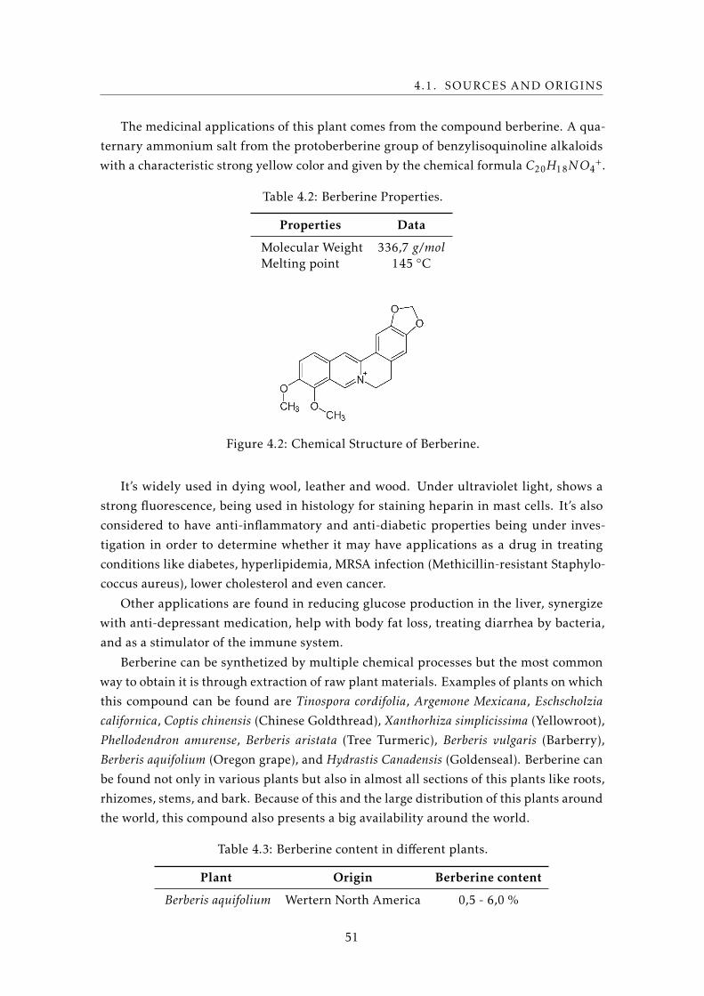
4.1. SOURCES AND ORIGINS
The medicinal applications of this plant comes from the compound berberine. A qua-
ternary ammonium salt from the protoberberine group of benzylisoquinoline alkaloids
with a characteristic strong yellow color and given by the chemical formula C20H18NO4+.
Table 4.2: Berberine Properties.
Properties Data
Molecular Weight 336,7 g/molMelting point 145 ◦C
Figure 4.2: Chemical Structure of Berberine.
It’s widely used in dying wool, leather and wood. Under ultraviolet light, shows a
strong fluorescence, being used in histology for staining heparin in mast cells. It’s also
considered to have anti-inflammatory and anti-diabetic properties being under inves-
tigation in order to determine whether it may have applications as a drug in treating
conditions like diabetes, hyperlipidemia, MRSA infection (Methicillin-resistant Staphylo-
coccus aureus), lower cholesterol and even cancer.
Other applications are found in reducing glucose production in the liver, synergize
with anti-depressant medication, help with body fat loss, treating diarrhea by bacteria,
and as a stimulator of the immune system.
Berberine can be synthetized by multiple chemical processes but the most common
way to obtain it is through extraction of raw plant materials. Examples of plants on which
this compound can be found are Tinospora cordifolia, Argemone Mexicana, Eschscholziacalifornica, Coptis chinensis (Chinese Goldthread), Xanthorhiza simplicissima (Yellowroot),
Phellodendron amurense, Berberis aristata (Tree Turmeric), Berberis vulgaris (Barberry),
Berberis aquifolium (Oregon grape), and Hydrastis Canadensis (Goldenseal). Berberine can
be found not only in various plants but also in almost all sections of this plants like roots,
rhizomes, stems, and bark. Because of this and the large distribution of this plants around
the world, this compound also presents a big availability around the world.
Table 4.3: Berberine content in different plants.
Plant Origin Berberine content
Berberis aquifolium Wertern North America 0,5 - 6,0 %
51

CHAPTER 4. BERBERINE - SOURCES AND EXTRACTION
Hydrastis canadensis North America 0,5 – 6,0 %Berberis aristata India/Nepal 3,18 %Berberis Tinctoria India 1,46 %Phellodendron amurense Asia 0,65 %Tinospora cordifolia India 0,035 %Argemone mexicana Mexico 0,05 %
As it’s possible to understand by the table above, even though berberine can be found
and obtain in almost all over the world, when it comes to pharmaceutical and industrial
applications the amount of this compound that can be found in most plants is very small
limiting the types of processes that can be used on the industrial scale due to the invest-
ment necessary and amount of raw material necessary in order to obtain a significant
amount of this compound. As it was mentioned before, the most common plant possess-
ing this type of compound is Berberis vulgaris, having some studies revealed an amount of
berberine in this plant in the order of 6%. This means that not only is a plant that exists
with a high distribution but also the amount of berberine discovered in the literature
suggests that could be close of some practical industrial applications.
4.2 Experimental Part
4.2.1 Materials
The root bark of Berberis vulgaris was obtained from a polish company called Nanga,
and the material had its origin from Pakistan. Berberine chloride form was purchased
from Sigma Aldrich. CO2 in its liquid form was bought from The Linde Group (Purity:
99.995%).
Table 4.4: Materials used.
Name of Reagent Units Unit Size Company
Berberis vulgaris 10 50 g NangaBerberine chloride 1 5 g Sigma AldrichCarbon dioxide 2 20 kg The Linde Group
4.2.2 Supercritical Fluid Extraction Systems
The experimental part was divided into the use of two different supercritical extraction
systems which were chosen based on the objective for each stage of the work. The systems
considered were a dynamic and static extraction, in which the first would be used to study
the process parameters and the second one to attempt extracting the target compound.
52

4.2. EXPERIMENTAL PART
4.2.2.1 Dynamic System
A dynamic extraction system consists on a constant flow of fresh solvent going through
the plant material extracting the compounds of interest. This system was mainly used for
studying the effects of the different process parameters.
This system operates with a pump for CO2 which is possesses an internal cooling
system, an extractor, a heater, a pressure control valve and two CO2 supply tanks. The
amount of CO2 used during the several experiments is controlled in order to make an
estimate on when to change to the second cylinder. When it comes to the extractor this
is divided into two main sections: an exterior metal vessel and an inner grid extraction
vessel.
The exterior vessel possesses the dimensions of 250 mm in length and 10,2 mm in
diameter. It possesses a thicker wall in order to sustain the high pressures which is
exposed, allowing the extraction of the raw material which is put inside. This exterior
vessel is submersed in a water bath which is warmed to the desired temperature by a
heater.
Figure 4.3: Exterior extraction vessel.
As for the inner vessel, the dimensions are 150 mm in length and 8 mm in diameter
with a grid of mesh 100 (0,15 mm). This inner vessel will contain the milled plant material
and then will be sealed using cotton wool.
Figure 4.4: Inner extraction vessel.
A back pressure regulator valve is used to control the pressure in the system. The
collection is made at room temperature and atmospheric pressure by simple system
53

CHAPTER 4. BERBERINE - SOURCES AND EXTRACTION
depressurization. The valve sits on top of a heater in order to avoid a clog caused by the
depressurization of the CO2.
Figure 4.5: Pressure control valve.
Temperature and pressure are controlled through two digital screens which are con-
nected to two sensors. The pressure sensor is connected to the main tubes were the
supercritical CO2 passes and the temperature sensor is put inside of the water bath.
Figure 4.6: Digital screens giving the values of temperature (oC) and pressure (bar).
The apparatus was design in order to perform extraction reactions using only CO2
as solvent. If co-solvents wanted to be used the system could be adapted by simply
introducing a second pump which would be responsible for introducing the organic
solvents into the extraction system.
Figure 4.7: Design Dynamic Supercritical Extraction System.
54

4.2. EXPERIMENTAL PART
4.2.2.2 Static System
This type of system was selected in order to collect as much powder of the target com-
pound as possible. The main advantage of this type of system is the fact it possesses a
bigger volume (V = 1,2 L) allowing the use of more plant material which would translate
in a higher amount of extract obtained.
This system is composed by a steel reactor, an oven, an agitation system and a system
of valves for both pressurization and depressurization of the system. The steel reactor has
a cylindrical shape and also possesses a thick wall in order to sustain the high pressure
inside.
Figure 4.8: Type of reactor used in static extraction.
This reactor is put inside an oven which will control the temperature inside the reactor.
The oven has also a cylindrical shape and the reactor is put through a hole that exists in
the center of it. The temperature is indicated through digital monitors and it presents the
values of temperature inside and outside of the reactor.
Figure 4.9: Oven for reactor temperature control.
55

CHAPTER 4. BERBERINE - SOURCES AND EXTRACTION
The pressure is indicated through an analogic indicator. The depressurization is made
at normal temperature and pressure and can be done by using organic solvents or not.
Figure 4.10: Analogic pressure indicator.
The system apparatus was also design to only operate with supercritical CO2 but it
would be possible to also operate using co-solvents as long another pump was added.
4.2.3 Extraction Process
4.2.3.1 Extraction in Dynamic Mode
The extraction process using a dynamic system was performed using several types of
conditions, having pressures in the range of 70 to 250 bar and testing at temperatures of
40oC and 60oC. The extraction process starts by first milling the plant material. The root
bark of Berberis vulgaris is characterized by its yellowish color and strong smell.
Figure 4.11: Example of non milled root bark.
The milling process was done using a coffee grinder (Sencor SCG 1050WH / SCG
1050BK). After being milled the material is then sieved in order to ensure that only a
specific material size would go into the extractor. The sieve was made using a net with
56

4.2. EXPERIMENTAL PART
the size of mesh 22 (0,8 mm). Usually the sample would have to go more than one time
through the sieve in order to guarantee that almost no dust was introduced into the
extractor.
Figure 4.12: Example of milled material.
The material is put inside the inner vessel which acts as a “basket” for the sieved plant
material in an amount of around 2 grams. The fact that the inner vessel is composed by a
net of a smaller size also helps to make a second barrier in which the dust particles that
stay in the plant material can be removed. The way the inner vessel is filled goes through
three main stages:
1. Weight the vessel alone without any plant material.
2. Weight the vessel now with the plant material in it.
3. Weight the full vessel already sealed with the cotton wool.
By the end of this stage it’s possible to know the size of the vessel, the amount of
material inside of the vessel and the weight of the cotton wool. Another important factor
is that because this inner vessel was made using a net material, there were some difficulties
in its construction. After some extraction the vessel started to give in so by using tape the
integrity of the inner vessel was maintained.
Then, after all the valves being closed and checked, the CO2 tank is open and the
pump activated right after that. The CO2 in the tank is in its liquid form (under pressure),
and when the valve is open the liquid is sucked into the pump and introduced into the
system. As it was mentioned before, the pump possesses a cooling system that allow
the solvent to remain liquid turning the pumping more effective. The pump used was a
metering one, allowing this way to establish a constant flow of 10 ml/min, which is the
equivalent of 5 g/min. The limitations of this pump are present mostly bellow and at the
critical point, where the gas and liquid CO2 do not allow it to be 100% efficient. Only
57

CHAPTER 4. BERBERINE - SOURCES AND EXTRACTION
after the critical point, at supercritical state, the pump can be efficient allowing a steady
rise in pressure.
After leaving the pump and achieve the required pressure, the fluid goes through a
serpentine which was also immersed in water so that when the fluid reaches the extractor
it has the pressure and temperature pretended.
Figure 4.13: Serpentine used.
Now in the supercritical state, CO2 goes through the plant material inside the extrac-
tor allowing the extraction of certain compounds. The temperature in the extractor is
controlled by the temperature in the hot water bath.
The pressure of the entire system is controlled by a back pressure valve which further
allows the collection of the extract by depressurization at normal temperature and pres-
sure. Actually, every time there was a change in the pressure used for the extraction the
valve had to be regulated prior in order to keep that specific pressure along the entire
extraction time. The measurements were made at the end each hour by stopping the
process and remove the sample. Then, the sample would be introduced again into the
extractor and the all process restarted with a total extraction time of around four hours.
Figure 4.14: Apparatus used for dynamic extraction.
58

4.2. EXPERIMENTAL PART
4.2.3.2 Extraction in Static Mode
As it was already mentioned, the propose of using this extraction system was to use more
plant material in a hope to obtain a larger quantity of extract. The first thing to do also
passes by milling the plant material using the same sieve has before with a grid size of
mesh 22 (0,8 mm). The amount of material which was used for this type of extraction was
around 22 grams and the vessel in which the material was introduced was also different
from the one used in the dynamic extraction.
In this case, the vessel was more like a small bag made of an elastic nylon net with a
net size of DEN 20, which still allowed some residual dust to escape. The bag was closed
by making a node and making sure that all the material was packed.
Figure 4.15: Bag containing plant material.
Then, the bag full of plant material was suspended inside the reactor vessel and
completely sealed. The CO2 tank is open and the pump is turn on right after it allowing
the pressure to build up inside the reactor. Then the stirring system was turn on to 100
rpm allowing to steer the fluid inside and help with the extraction process. The pressure
and temperature conditions used were 130 bar and 70oC respectively. The low conditions
applied have to do with the limitations imposed by the equipment. At the time of the
experiments the pump was constantly malfunctioning and barley rising the pressure in
the system. A solution found to get more pressure was to stop the pump and increase the
temperature, allowing an increase of pressure as the temperature also increases.
The extraction occurred for two straight hours and the collection was made by de-
pressurization at normal temperature and pressure. It’s possible to see that when there’s
a depressurization of CO2 that the temperature goes down and it looks like the vessel
freezes. A cotton wool is put on the entry of the vessel so if any residual splash happen it
still gets retained inside the vessel.
The collection vessel and the reactor itself were then rinsed with acetone in order to
collect any residual extract that was not removed by the depressurization. The process
of depressurization has to be done slowly in order to control the flow of CO2 leaving the
system and not lose any extract in the process.
59

CHAPTER 4. BERBERINE - SOURCES AND EXTRACTION
Figure 4.16: Apparatus used for static extraction.
Figure 4.17: Collection by depressurization.
4.2.4 Water content
The water content of the Berberis vulgaris was investigated in order to see if moisture was
an important factor when it came to the extraction of this plant material. The root bark
was divided into two samples of 2 grams each, being one of them milled and the other
just like it came from the supplier. Both samples were put inside an oven at 120oC for
two hours. When it comes to the milled sample the water content was found to be 0,20%.
This shows that the influence of this parameter in the extraction is not significant. For the
not milled sample the water content was 0,21% which also seems to be non-significant.
60

4.3. ANALYTICAL METHOD
Figure 4.18: Samples for analyzes of water content.
4.3 Analytical Method
The analytical stage allows to guarantee if an extraction process was successful in remov-
ing from the plant material a certain compound by identify it in the extract and in what
quantity. As it already been mentioned, there are several methods of analyzing extraction
products from GC/MS to HPLC, depending on the objective of the work itself. In the
case of berberine the first option to analyze it was to use HPLC in the first place. Some
literature was found were berberine analyses is described and from there a protocol could
be developed with that objective.
Table 4.5: Literature data on berberine analytical methods.
Method Reference
HPLC [87]HPLC [88]HPLC [89]HPLC [66]HPLC [67]HPLC [90]HPLC [91]
With the shortage of time available to perform more experiments, it was thought that
a simpler analysis could be made in order to prove that berberine was in fact extracted.
With that in mind, the proposed technique was differential scanning calorimetry (DSC)
which would allow to compare the extract with a reference in terms of how much heat is
necessary to raise the temperature of each of them.
Due to a very low amount of extract obtained even this method wasn’t possible to be
performed leaving only certain properties like color and smell suggesting the presence of
berberine in the extract.
61

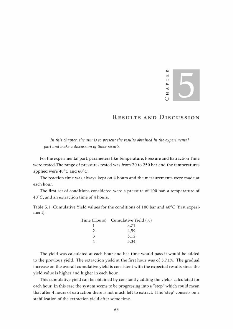
Chapter
5Results and Discussion
In this chapter, the aim is to present the results obtained in the experimentalpart and make a discussion of those results.
For the experimental part, parameters like Temperature, Pressure and Extraction Time
were tested.The range of pressures tested was from 70 to 250 bar and the temperatures
applied were 40oC and 60oC.
The reaction time was always kept on 4 hours and the measurements were made at
each hour.
The first set of conditions considered were a pressure of 100 bar, a temperature of
40oC, and an extraction time of 4 hours.
Table 5.1: Cumulative Yield values for the conditions of 100 bar and 40oC (first experi-ment).
Time (Hours) Cumulative Yield (%)1 3,712 4,593 5,124 5,34
The yield was calculated at each hour and has time would pass it would be added
to the previous yield. The extraction yield at the first hour was of 3,71%. The gradual
increase on the overall cumulative yield is consistent with the expected results since the
yield value is higher and higher in each hour.
This cumulative yield can be obtained by constantly adding the yields calculated for
each hour. In this case the system seems to be progressing into a “step” which could mean
that after 4 hours of extraction there is not much left to extract. This "step" consists on a
stabilization of the extraction yield after some time.
63
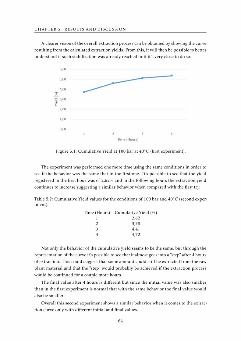
CHAPTER 5. RESULTS AND DISCUSSION
A clearer vision of the overall extraction process can be obtained by showing the curve
resulting from the calculated extraction yields. From this, it will then be possible to better
understand if such stabilization was already reached or if it’s very close to do so.
Figure 5.1: Cumulative Yield at 100 bar at 40oC (first experiment).
The experiment was performed one more time using the same conditions in order to
see if the behavior was the same that in the first one. It’s possible to see that the yield
registered in the first hour was of 2,62% and in the following hours the extraction yield
continues to increase suggesting a similar behavior when compared with the first try.
Table 5.2: Cumulative Yield values for the conditions of 100 bar and 40oC (second exper-iment).
Time (Hours) Cumulative Yield (%)1 2,622 3,783 4,414 4,72
Not only the behavior of the cumulative yield seems to be the same, but through the
representation of the curve it’s possible to see that it almost goes into a "step" after 4 hours
of extraction. This could suggest that some amount could still be extracted from the raw
plant material and that the "step" would probably be achieved if the extraction process
would be continued for a couple more hours.
The final value after 4 hours is different but since the initial value was also smaller
than in the first experiment is normal that with the same behavior the final value would
also be smaller.
Overall this second experiment shows a similar behavior when it comes to the extrac-
tion curve only with different initial and final values.
64

Figure 5.2: Cumulative Yield at 100 bar at 40oC (second experiment).
The next experiment was performed by keeping the temperature at 40oC and the
extraction time at 4 hours. The only condition which changed was the pressure to 150
bar. Just like the experiment before, the first hour records a superior extraction yield
being in this case of 2,57%. Again the behavior seems to be consistent with the previous
experiments.
Table 5.3: Data from 150 bar and 40oC (first experiment).
Time (Hours) Cumulative Yield (%)1 2,572 3,873 5,034 6,10
When presenting the cumulative yield curve is possible to see a completely different
behavior from the other cases since it doesn’t suggest to be even close to a step.
It behaves more like a straight line suggesting that it could be extracted much more
from the raw plant material. If this was an isolated case, than it would be a plausible
explanation but when looking at the previous cases and what would be expected theoret-
ically, other scenarios could be drawn from this data.
One plausible alternative would be of experimental error. Extraction from raw plant
materials is a difficult system being difficult to maintain the same conditions since some
plant material can be lost even by just introducing or removing the extraction vessel.
Other possible explanation has to do with the supercritical system in itself. Supercrit-
ical systems are only now being more studied and so solid models don’t exist yet.
This causes to be hard to obtain the exact same values for all experiments and that
even a small change in the process conditions could cause a large difference in the end
results.
65

CHAPTER 5. RESULTS AND DISCUSSION
Figure 5.3: Cumulative Yield at the conditions of 150 bar and 40oC (first experiment).
The second experiment, performed with the same conditions, showed a calculated
yield at the first hour of 2,69%. This value, even that slightly higher that the previous
one, makes that the curve starts around the same range of values allowing to, considering
a similar behavior, to obtain a final value after 4 hours within the same range of values as
the previous one.
In reality what happens is a final value considerably smaller that it the previous
case. This might suggest that something went wrong in the first experiment using this
conditions, resulting in a significantly increase of the calculated yield.
Table 5.4: Data from 150 bar and 40oC (second experiment).
Time (Hours) Cumulative Yield (%)1 2,692 3,573 4,084 4,46
The cumulative yield curve shows in this case a behavior a little different since it tends
more into a step that in the first case. Like it was previously suggested, this fact might
indicate a less significant amount existing to be extract after the 4 hours of extraction.
Even so, the duration of the extraction process is still proving to be insufficient for the
temperature of 40oC.
In the end is possible to see that the overall behavior still shows a tendency to go up
instead of stabilizing within the 4 hours. On the other hand, the final yield obtained for
this particular case is much lower than in the first experiment, what can be explained by
the different behavior of the cumulative curve.
It would be expected that if the extraction would continue for more than 4 hours that
it would eventually come to stabilize.
66

Figure 5.4: Cumulative Yield at the conditions of 150 bar and 40oC (second experiment).
In the next set of conditions, the temperature and extraction time were kept the same
changing only the pressure to 200 bar. In this experiment the behavior of the obtained
yield started the same as the others but after the third hour it completely changed.
The large increase on the calculated yield could have been caused by some experimen-
tal issue as its been mentioned before.
The extractions performed so far clearly suggest that it’s very difficult to completely
control the experimental factors such as the distribution of the material. In fact, because
the inner vessel was composed by a grid, there was the possibility that the smallest
particles would leave the vessel when this was introduced or removed from the exterior
vessel.
Table 5.5: Data from 200 bar and 40oC (first experiment).
Time (Hours) Cumulative Yield (%)1 3,532 4,593 4,784 5,34
When it comes to the cumulative yield curve, it’s possible to see that in the first 3 hours
the behavior suggests that it’s tending to a step but after the fourth hour it rises again.
This could be explained by some loss in material when the inner vessel was removed
causing a higher increase in weight loss of the sample.
Experimental issues can only be solved by the acquirement of experience by the oper-
ator and so the development of a method which allows to minimize such mistakes. The
familiarity of the operator with the equipments is also an important factor which could
cause divergences on the final results.
For this reason is clear that the first experiments need to be looked at with care since
67

CHAPTER 5. RESULTS AND DISCUSSION
those experiments are the ones on which the operator had less experience.
Figure 5.5: Cumulative Yield at the conditions of 200 bar and 40oC (first experiment).
On the second try with this conditions it is possible to see that the values obtained
make more sense than in the previous experiment. The yield obtained at the first hour
was 2,73%.
The yield in each hour continuously increases and there was no sudden increase of
yield which could suggest that differently from the previous experiment there was no
significant loss of weight by the material sample.
After the 4 hours of extraction the yield final value obtained was 4,62%. This value was
considerably smaller when compared to the previous yield obtained on the last extraction
process hour.
This low value can be explained not only in terms of the weight loss of the sample but
also in terms of the behavior of the curve and its initial value. The initial value in this
case is much smaller as well which leads to a curve with an similar behavior to have a
smaller value on the final value as well.
Table 5.6: Data from 200 bar and 40oC (second experiment).
Time (Hours) Cumulative Yield (%)1 2,732 3,763 4,284 4,62
As for the cumulative curve, it’s clear that the behavior tends almost into a step. This
result comparing to the one got in the previous experiments makes more sense and gives
a better explanation for the process behavior in this conditions. It’s possible to see a curve
being formed as an alternative to the weird behavior shown at the previous experiment.
Again it’s possible to see that at the temperature of 40oC, 4 hours are not enough to
achieve the "step" and to extract everything that is possible from the plant material.
68

Figure 5.6: Cumulative Yield at the conditions of 200 bar and 40oC (second experiment).
On the set of conditions of 250 bar and 40oC, the experiment was performed for 4
hours presenting different results that the previous experiments. The yield after the first
hour is consistent with the values obtained before, possessing a behavior very similar ex-
cept at the third hour were the yield increased instead of being smaller than the previous
one. Again this increase in yield could have resulted of a mass lost when introducing or
removing the inner vessel from the extractor. This would result in a larger mass difference
and by consequence a bigger yield than expected.
Table 5.7: Data from 250 bar and 40oC (first experiment).
Time (Hours) Cumulative Yield (%)1 2,832 4,083 5,334 5,62
When it comes to the cumulative graph is possible to see that the behavior is mostly a
constant growth of the extraction yield presenting a straight line. This behavior last for
the first 3 hours tending closer to a step on the fourth hour.
It’s clear that the shape of the curve is not similar to the curves obtained so far. Until
now, the curves have displayed a gradual increase of yield resulting on an actual curve
tending into a step.
This case on the other hand, presents a rapid and constant increase of the yield, being
represented by a straight line as it was mentioned before.
Although, after the fourth hour the behavior seems to be quite similar to what was
seen before, suggesting that after the 4 hours there was not much left to extract just like
in the previous cases.
69

CHAPTER 5. RESULTS AND DISCUSSION
Figure 5.7: Cumulative Yield at the conditions of 250 bar and 40oC (first experiment).
The experiment was done one more time in order to check the first results obtained.
The yield obtained in the first hour is slightly higher than in the first experiment pre-
senting a value of 3,43%. The general behavior is more consistent with all previous
experiments on other conditions with a very steep fall in yield between the first and
second hour, followed by a constant low in yield on the course of the 4 hours.
Table 5.8: Data from 250 bar and 40oC (second experiment).
Time (Hours) Cumulative Yield (%)1 3,432 4,423 4,814 5,07
Regarding the cumulative graph is possible to see that the behavior is no longer a
constant rise in yield but instead it tends closer to step has times passes. The final yield
is also lower than in the first experiment even if the first value was higher what can be
explained by the curve shape.
In this case it’s possible to see a clear improvement when compared to the first exper-
iment using this conditions. The behavior of the curve looks consistent to the previous
experiments and after 4 hours seems to be around the same range of values.
There’s a gradual increase of the yield but its still possible to see a straight line behav-
ior between the second and fourth hour of experiment.
It’s also important to mention the value obtained after the first hour its superior to
the one obtained at the first experiment with this conditions. On the other hand the final
value after four hours is smaller what goes against what would be expected since that
if the initial value is high then the final one would be expected to be higher than in the
previous cases.
70

Figure 5.8: Cumulative Yield at the conditions of 250 bar and 40oC (second experiment).
Having all the experimental data at 40oC presented, it’s important to compare all the
results obtained at different pressures. It’s possible to see that there’s no clear effect of
the pressure on the process when temperature is kept constant at 40oC. At the pressure
of 250 bar the extraction yield is higher but the value is still not as significant to consider
a real influence of pressure since the values are very close to each other.
It’s also possible to see that the curves have mostly the same behavior, with the yields
in each hour practically similar.
Figure 5.9: Comparison of the effect of different pressures at the temperature of 40oC.
71
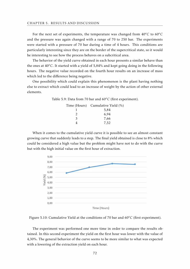
CHAPTER 5. RESULTS AND DISCUSSION
For the next set of experiments, the temperature was changed from 40oC to 60oC
and the pressure was again changed with a range of 70 to 250 bar. The experiments
were started with a pressure of 70 bar during a time of 4 hours. This conditions are
particularly interesting since they are on the border of the supercritical state, so it would
be interesting to see how the process behaves on a subcritical area.
The behavior of the yield curve obtained in each hour presents a similar behave than
the ones at 40oC. It started with a yield of 5,84% and kept going doing in the following
hours. The negative value recorded on the fourth hour results on an increase of mass
which led to the difference being negative.
One possibility which could explain this phenomenon is the plant having nothing
else to extract which could lead to an increase of weight by the action of other external
elements.
Table 5.9: Data from 70 bar and 60oC (first experiment).
Time (Hours) Cumulative Yield (%)1 5,842 6,943 7,664 7,52
When it comes to the cumulative yield curve it is possible to see an almost constant
growing curve that suddenly leads to a step. The final yield obtained is close to 8% which
could be considered a high value but the problem might have not to do with the curve
but with the high initial value on the first hour of extraction.
Figure 5.10: Cumulative Yield at the conditions of 70 bar and 60oC (first experiment).
The experiment was performed one more time in order to compare the results ob-
tained. In this second experiment the yield on the first hour was lower with the value of
4,30%. The general behavior of the curve seems to be more similar to what was expected
with a lowering of the extraction yield on each hour.
72

Table 5.10: Data from 70 bar and 60oC (second experiment).
Time (Hours) Cumulative Yield (%)1 4,302 5,743 6,264 6,33
When it comes to the cumulative extraction curve it’s possible to see that it tends into
a step and with a final yield much lower than in the first experiment.
The fact that it tends into a step goes against what was expected since this is the lowest
pressure tested.
Figure 5.11: Cumulative Yield at the conditions of 70 bar and 60oC (second experiment).
In the next experiment the pressure was changed to 100 bar keeping the temperature
and extraction time constant. The yield at the first hour was 5,10%, keeping to go down
until the third hour. At the fourth hour there’s an increase in yield which could mean that
in some way an amount of material was lost from the inner extractor, causing a larger
mass difference.
Table 5.11: Data from 100 bar and 60oC (first experiment).
Time (Hours) Cumulative Yield (%)1 5,102 7,203 7,374 8,23
The cumulative yield shows a weird behavior since that at the second hour a step
73

CHAPTER 5. RESULTS AND DISCUSSION
seemed to be forming, and then with the increase in yield that same step disappeared on
the fourth hour of extraction. It also achieves large final yields which could be influenced
by some experimental failure.
Figure 5.12: Cumulative Yield at the conditions of 100 bar and 60oC (first experiment).
The results obtained in the first experiment are considered weird when compared
with the previous experiences which made that the experiment had to be performed one
more time in order to compare the results obtained.
Although in this second experiment things became even more incoherent since the
behavior of the curves was even more different than usual with a massive increase of yield
in just 2 hours of extraction. After that, the mass increased in very small percentages
making this behavior completely different from anything that was observed until now.
Table 5.12: Data from 100 bar and 60oC (second experiment).
Time (Hours) Cumulative Yield (%)1 6,512 6,893 6,624 6,38
Regarding the cumulative yield, it’s clear that the behavior is completely different
from what usually seen, with the yield actually going down instead of the normal behav-
ior.
In fact, is possible to see that none of the values make any sense. From the start the
yield obtained at the first hour is just too high when compared to all the other experi-
ments.
Also, the fact that it goes up and then constantly down also presents a major difference
to the previous experiments.
74

Figure 5.13: Cumulative Yield at the conditions of 100 bar and 60oC (second experiment).
Since the results obtained were again so strange, it was decided to perform this exper-
iment one more time, but unfortunately it was only possible to do so for 3 hours since the
equipment did not allow for the usual 4 hours of extraction to be performed.
In this 3 hours experiment it’s possible to see a more general behavior in which the
yield goes up more at each hour of extraction and it seems that there were no major
difficulties with the extraction process.
Table 5.13: Data from 100 bar and 60oC (third experiment).
Time (Hours) Cumulative Yield (%)1 4,252 5,723 6,40
When it comes to the cumulative yield is possible to see also a tendency to stabilize
even though only 3 hours have passed. By the behavior of the curve it’s possible to assume
that it would be even closer to a step closer to 7%. The initial yield value also presents
the smallest of all obtained in these conditions and the closest one to what would be the
common values for the yield at the first hour of extraction.
Like it was mentioned before, there was no time to perform this third try since the
equipment didn’t allow the conditions to be achieve in a faster way so these results even
that are not perfect are an approximation of what could be expected at this operating
conditions.
It is very interesting to see how can similar experiments present such different re-
sults.This shows how hard it is to control the behavior of these systems and how the
search for new models is important for a better understanding and application of super-
critical fluids.
75

CHAPTER 5. RESULTS AND DISCUSSION
Figure 5.14: Cumulative Yield at the conditions of 100 bar and 60oC (third experiment).
New conditions were then applied by changing the pressure to 150 bar. Temperature
and extraction time were kept the same. In a first experiment using these conditions it’s
possible to see an expected behavior and also a lower value after 1 hour of extraction
(3,54%).
The final value, 6,42%, also seems to be consistent with the general data obtained so
far for this temperature.
Even if it was not very clear when using a pressure of 100 bar, when considering all
the data obtained so far at the temperature of 60oC, it is possible to see that in the 4 hours
of extraction time there is a tendency to achieve the "step". In this case, that tendency to
a stabilization is also quite clear.
Table 5.14: Data from 150 bar and 60oC (first experiment).
Time (Hours) Cumulative Yield (%)1 3,542 5,433 6,124 6,42
As it was mentioned before, the cumulative curve doesn’t present much surprises
since its behavior is within the expected and tending to a step after 4 hours extraction.
The gradual growth of the yield obtained and the small initial value may suggest that
in this case everything went well and that there were no significant influences, which
would destabilize the overall extraction system.
Also, as it was mentioned above, a stabilization of the extraction yield after 4 hours
would suggest a tendency for the extraction to be faster at this temperature causing in
the various pressures a similar behavior in only 4 hours of running. On the other hand,
at 40oC it was clear that four hours was not enough to achieve that step.
76

Figure 5.15: Cumulative Yield at the conditions of 150 bar and 60oC (first experiment).
As a normal procedure, in order to confirm the values, the experiment was performed
once more. In this second experiment is possible to see that again at the fourth hour
there’s a slight increase in the extraction yield witch causes a deviation of the curves
behavior. Again this can be explained by some sudden mass lost which could cause these
abnormalities.
Both initial and final value can be considered within range when compared with the
other experiments at 60oC.
Table 5.15: Data from 150 bar and 60oC (second experiment).
Time (Hours) Cumulative Yield (%)1 5,122 6,053 6,234 6,55
When it comes to the cumulative yield is possible to see the change on the normal
curve behavior at the fourth hour, causing a final yield of close to 7%. The curve seems to
tend into a stabilization between the second and third hour which would suggest a very
quick extraction.
The problem itself might not be on the value obtained at the fourth hour of extraction
but yes on the third one, causing a slight depression and by result the different curve
behavior presented.
Again, a plausible explanation for this is the inner vessel letting some of the smaller
particles get way by the friction between the inner and exterior vessel. Even being very
careful in the stages of milling, sieving, filling the inner vessel with material, and also
taking and introducing it into the extraction vessel, a small complication or mass lost
could cause a massive change in the curves behavior.
77

CHAPTER 5. RESULTS AND DISCUSSION
Figure 5.16: Cumulative Yield at the conditions of 150 bar and 60oC (second experiment).
Since the results of the second experiment were not very reliable, a third experiment
using the same conditions was performed. In this case the same problem appears, having
a high initial yield and a strange curve behavior with a high yield increase at the fourth
hour.
Table 5.16: Data from 150 bar and 60oC (third experiment).
Time (Hours) Cumulative Yield (%)1 5,362 5,943 6,104 6,32
The cumulative curve presents an even weirder behavior by continuing to go up for
the entire 4 hours. There are two main section which deserve a more careful analysis
being one of them between the first and second hour, and the other between the third and
fourth hour. As it was mentioned before, on the fourth hour there is a significant increase
of the yield obtained which could be related to some kind of problem at that moment or
be result of a problem at the third hour, causing a depression and a weird behavior of the
curve.
Between the first and second hour of extraction there is also a big increase but when
looking at the previous experiments is possible to see that such behavior is normal. Even
that slightly high, the first value is within range when compared with the previous exper-
iments.
Extraction using a continuous supercritical system is difficult in a sense that’s a com-
plex system in which small alteration in the parameters could cause major differences
and so it becomes difficult to achieve replicated results. Also, as it was mentioned before,
the material itself is hard to control so it could also cause some differences in the final
78

results.
Figure 5.17: Cumulative Yield at the conditions of 150 bar and 60oC (third experiment).
The conditions were then changed again to a pressure of 200 bar keeping everything
else constant. Over the extraction time, in each hour the yield values increase at different
rates becoming in line with the previous experiments for the first 3 hours.
Again, in the fourth hour, the extraction yield becomes negative, causing the value of
cumulative yield to go down. This negative value might imply that the sample gained
weight.
Even though the values are in the same range as the ones in previous experiments,
they are still considered low values. The suppose weight gain could be caused by the
influence of the humidity in the air, which could enter the raw material and cause an
increase of mass.
Table 5.17: Data from 200 bar and 60oC (first experiment).
Time (Hours) Cumulative Yield (%)1 4,442 5,863 6,124 6,06
The cumulative yield curve shows a behavior similar to previous experiments ending
up achieving a step.
This experiment just like the others before, was also done one more time but the
results can’t be shown since this experiment has a methodology error. The sample was
left at the open the entire night which was seen later that would affect the end results.
Since the methodology is not corrected that second experiment shouldn’t be shown since
it’s not in conformity with all the others.
79
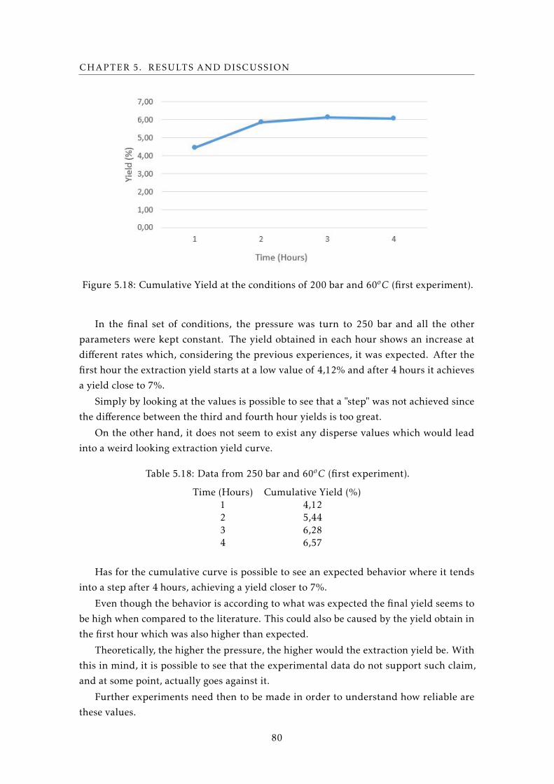
CHAPTER 5. RESULTS AND DISCUSSION
Figure 5.18: Cumulative Yield at the conditions of 200 bar and 60oC (first experiment).
In the final set of conditions, the pressure was turn to 250 bar and all the other
parameters were kept constant. The yield obtained in each hour shows an increase at
different rates which, considering the previous experiences, it was expected. After the
first hour the extraction yield starts at a low value of 4,12% and after 4 hours it achieves
a yield close to 7%.
Simply by looking at the values is possible to see that a "step" was not achieved since
the difference between the third and fourth hour yields is too great.
On the other hand, it does not seem to exist any disperse values which would lead
into a weird looking extraction yield curve.
Table 5.18: Data from 250 bar and 60oC (first experiment).
Time (Hours) Cumulative Yield (%)1 4,122 5,443 6,284 6,57
Has for the cumulative curve is possible to see an expected behavior where it tends
into a step after 4 hours, achieving a yield closer to 7%.
Even though the behavior is according to what was expected the final yield seems to
be high when compared to the literature. This could also be caused by the yield obtain in
the first hour which was also higher than expected.
Theoretically, the higher the pressure, the higher would the extraction yield be. With
this in mind, it is possible to see that the experimental data do not support such claim,
and at some point, actually goes against it.
Further experiments need then to be made in order to understand how reliable are
these values.
80

Figure 5.19: Cumulative Yield at the conditions of 250 bar and 60oC (first experiment).
In order to compare the obtained values, the experiment was performed once more.
Analyzing the yields obtained in each hour of extraction it’s possible to confirm a similar
behavior of the curve which tends into a "step".
When it comes to the values obtained it is possible to see that it starts with a slightly
higher value, 4,53%, and curiously ends with a much smaller value, 5,87%, when com-
pared with the previous experiments.
By looking at the values it does not seem to exist anything out of the ordinary for the
first 3 hours, with a steady increase of the extraction yield.
On the other hand, this happens only in those first 3 hours since that at the fourth
hour there’s a very small increase of mass which leads to the value of the yield to be
negative. This results in a decrease of the cumulative extraction yield.
Table 5.19: Data from 250 bar and 60oC (second experiment).
Time (Hours) Cumulative Yield (%)1 4,532 5,643 5,894 5,87
The cumulative yield curve presents an expected shape, tending into a step very
quickly. Even with the small mass increase, graphically it still looks like a step was
formed in a range closer to 6%.
As it was mentioned before, theoretically these were the best operating conditions
for extraction since they are a combination of highest temperature and pressure, so the
fact that it tends into a step in only 4 hours goes into that expectation. But we can forget
the fact that the extraction yield obtained after those 4 hours does not relate to that
perspective when compared with other pressures at the same temperature.
81

CHAPTER 5. RESULTS AND DISCUSSION
Figure 5.20: Cumulative Yield at the conditions of 250 bar and 60oC (second experiment).
The values obtained for the different pressures were then organized into one graph
so they could be compared and analyzed. Looking at the data is possible to see that all
the curves have almost the same behavior and that tend to very close values which leads
to think that there’s no significant influence of pressure in this type of process and rest
of set of conditions. The value of 100 bar was used at only three hours since that from
all the experiments performed with those conditions is the only one that makes sense or
allows a clear comparison with the other sets of pressure.
Figure 5.21: Comparison of different pressures at the temperature of 60oC.
Like it was mentioned before, one of the main ideas taken from this work is that
82

temperature might have a strong influence on the extraction process.
With this in mind, the temperatures of 40oC and 60oC were compared for each pres-
sure value considered.
In the case of 100 bar, is clear that at 60oC the cumulative yield shown suggest a better
extraction, achieving higher values.
Figure 5.22: Comparison of different temperatures at the pressure of 100 bar.
In the case of 150 bar the same relation is shown with a "step" being achieved much
faster and the yield values being much higher for the temperature of 60oC.
Figure 5.23: Comparison of different temperatures at the pressure of 150 bar.
Again for 200 bar is clear that such "step" is achieved much faster at 60oC. In fact, at
40oC the step is not even achieved within the four hours of extraction.
83

CHAPTER 5. RESULTS AND DISCUSSION
Figure 5.24: Comparison of different temperatures at the pressure of 200 bar.
In the case of 250 bar, again is possible to see this effect of the temperature on the
overall process. It’s probably one of the best cases to see the formation of the so called
"step", when compared with the slight increase of the yield at 40oC.
Figure 5.25: Comparison of different temperatures at the pressure of 250 bar.
This way, the effect of the temperature on the overall extraction process, suggests to
be highly significant considering all the data presented.
84

Chapter
6Conclusions
In this chapter, the aim is to present the main conclusions of the performedwork.
Medicinal plants possess many compounds which can be used for pharmaceutical
applications. Traditional extraction techniques were focused on using organic solvents or
apply conditions that would degrade compounds being of interest. For that reason, this
work was focused in application of supercritical fluid extraction to extract the medicinal
based compounds from raw materials. This innovative method allows a more environ-
mentally friendly extraction, which uses mild conditions to avoid compound degradation.
By using CO2 as solvent it is possible to remove its traces from the extract allowing to
obtain a pure product. A great interest was demonstrated to study supercritical fluid
extraction applied to raw plant materials because high quality extracts could be captured
from them to apply those compounds in multiple areas. From the presented study, the
following conclusions can be drawn:
1. The investigation was first focused on the plant Sassafras albidum with the main
purpose of safrole extraction. Due to legal reasons, it became impossible to acquire
the necessary compounds or even the raw plant material with a high content of
safrole since a license is required in order to work with these type of compounds.
Being impossible to proceed with the experimental part with this plant, provided
us to search for an alternative subject. There it was made a decision to focus on
investigation on another plant called Berberis vulgaris, with the objective of obtain-
ing the compound berberine. This required an additional time for ordering and
delivery of Berberis vulgaris, but our main purpose was to select this raw material
to shorten the time of ordering and delivery to minimum. Several experiments
85

CHAPTER 6. CONCLUSIONS
were performed in order to understand if the technique is valuable in this cases and
identify the influence of the process parameters.
2. The study focused on supercritical extraction allow to state that is a valuable method
for the extraction of the plant materials. According to mass differentiation the
extraction yields were calculated as to be from 4,46% to 8,23%, guarantying that
the extraction not only is possible but sufficient.
3. The influence of temperature in the supercritical fluid extraction process is visible
because higher temperature increased the extraction yield within the same extrac-
tion time. The investigated temperatures were 40oC and 60oC. The same extraction
time of four hours, at 60oC made the extraction process faster achieving higher
yields compared with the same conditions at 40oC.
4. The influence of pressure in the extraction process was found not to be significant.
At the temperature of 60oC, the experimental extraction curves tend mostly to the
same “step” values and present the same kind of behavior witch could indicate that
the change in pressure does not affect the extraction process. At 40oC on the other
hand, it seems to have a small influence on the extraction yields obtained but the
values are so close to each other that loses relevance. The influence of the extraction
time is clearly visible since, in all experiments, it was possible to see that the longer
the extraction process occurred, the more the curve would tend to a stabilization
of the extracted amount. The typical behavior observed is, has time passes, that
the differential yield presents a lower and lower value causing the cumulative yield
curve to progress into a “step”. This simply means that there is a maximum amount
of extract can be obtained and that the longer the extraction process occurs the more
the curve tends into that “step”. It can also suggest that the process is controlled by
the solute diffusion in the individual particles of the plant raw material and that an
increase in the extraction time corresponds to more mass transfer resistance.
5. The obtained yields are not referent to berberine in specific but to the overall yield
obtained by mass differentiation. Due to the high yield values obtained in the
first extraction hour, the content of water in the plant material was considered
to be significant. Importance of raw material studied as received or milled was
investigated as well. The water contents observed in both milled and received
materials were 0,20% and 0,21% respectively which leads to conclude that a large
portion of what was extracted in the first hour is related to plant compounds other
than water.The investigation was focused as well on recovering the powder. It is
possible to conclude that even using a static extraction system instead of a dynamic
one, containing a bigger volume (V = 1,2 L) and a larger amount of plant material as
a sample, the extraction was possible allowing through mass difference a yield close
to 3%. Powder was not obtained. Collection in acetone allowed to obtain a yellowish
liquid and a strong smell, the same like in the plant. These physical properties don’t
86

prove that berberine was present, but suggest that some residual amount might
exist. Differential scanning calorimetry (DSC) was selected to analyze the obtained
extract, by comparing the amount of heat necessary to increase the temperature of
the extract with a reference of pure berberine. Unfortunately, sufficient amount of
extract was not obtained in order to use this analytical method.
6. The application of supercritical extraction on the plant Berberis vulgaris showed
good results and high prospects for future studies. From the experiments per-
formed, it is clearly noticed that supercritical CO2 could be a good option for the
extraction of berberine from this plant. Nevertheless, this method will require more
development and improvement with the possible introduction of co-solvents in the
extraction process or develop an alternative analytical protocol such as with HPLC.
87

Bibliography
[1] P. Kenrick and P. R. Crane. The origin and early diversification of land plants. Acladistic study. Vol. 560. Smithsonian Institute Press Washington DC.: A cladistic
study. Smithsonian Institute Press, 1997.
[2] Plants. [Accessed: 24-July-2016]. url: https://en.wikipedia.org/wiki/Plant.
[3] R. Bentley and H. Trimen. “Medicinal plants”. In: Medicinal plants. J & A Churchill,
1981.
[4] B. B. Petrovska et al. “Historical review of medicinal plants’ usage”. In: Pharma-cognosy reviews 6.11 (2012), p. 1.
[5] Water distillation in the extraction of essential oils. [Accessed: 17-August-2016]. url:
http://www.essentialoils.co.za/water-distillation.htm.
[6] B. Abdul-Majeed, A. Hassan, and B. Kurji. “Extraction of Oil from Eucalyptus
Camadulensis Using Water Distillation Method”. In: Iraqi Journal of Chemical andPetroleum Engineering 14 (2013), pp. 7–12.
[7] W. Guan, S. Li, R. Yan, S. Tang, and C. Quan. “Comparison of essential oils of
clove buds extracted with supercritical carbon dioxide and other three traditional
extraction methods”. In: Food Chemistry 101.4 (2007), pp. 1558–1564.
[8] S. Périno-Issartier, C. Ginies, G. Cravotto, and F. Chemat. “A comparison of es-
sential oils obtained from lavandin via different extraction processes: ultrasound,
microwave, turbohydrodistillation, steam and hydrodistillation”. In: Journal ofChromatography A 1305 (2013), pp. 41–47.
[9] O. Nautiyal and K. Tiwari. “Extraction of dill seed oil (Anethum sowa) using
supercritical carbon dioxide and comparison with hydrodistillation”. In: Industrial& Engineering Chemistry Research 50.9 (2011), pp. 5723–5726.
[10] M. Khajeh, Y. Yamini, F. Sefidkon, and N. Bahramifar. “Comparison of essential
oil composition of Carum copticum obtained by supercritical carbon dioxide ex-
traction and hydrodistillation methods”. In: Food chemistry 86.4 (2004), pp. 587–
591.
89

BIBLIOGRAPHY
[11] M. A. Ferhat, B. Y. Meklati, and F. Chemat. “Comparison of different isolation
methods of essential oil from Citrus fruits: cold pressing, hydrodistillation and
microwave ‘dry’distillation”. In: Flavour and Fragrance Journal 22.6 (2007), pp. 494–
504.
[12] How Are Essential Oils Extracted? [Accessed: 14-August-2016]. url: http://www.
essentialoils.co.za/water-distillation.htm.
[13] M. R. Tellez, I. A. Khan, B. T. Schaneberg, S. L. Crockett, A. M. Rimando, and
M. Kobaisy. “Steam distillation–solid-phase microextraction for the detection of
Ephedra sinica in herbal preparations”. In: Journal of Chromatography A 1025.1
(2004), pp. 51–56.
[14] M. Z. Ozel and H. Kaymaz. “Superheated water extraction, steam distillation and
Soxhlet extraction of essential oils of Origanum onites”. In: Analytical and bioana-lytical chemistry 379.7-8 (2004), pp. 1127–1133.
[15] C Boutekedjiret, F Bentahar, R Belabbes, and J. Bessiere. “Extraction of rosemary
essential oil by steam distillation and hydrodistillation”. In: Flavour and FragranceJournal 18.6 (2003), pp. 481–484.
[16] F Chemat, M. Lucchesi, J Smadja, L Favretto, G Colnaghi, and F Visinoni. “Mi-
crowave accelerated steam distillation of essential oil from lavender: A rapid, clean
and environmentally friendly approach”. In: Analytica Chimica Acta 555.1 (2006),
pp. 157–160.
[17] A Donelian, L. Carlson, T. Lopes, and R. Machado. “Comparison of extraction of
patchouli (Pogostemon cablin) essential oil with supercritical CO 2 and by steam
distillation”. In: The Journal of Supercritical Fluids 48.1 (2009), pp. 15–20.
[18] A. Ammann, D. C. Hinz, R. S. Addleman, C. M. Wai, and B. W. Wenclawiak. “Su-
perheated water extraction, steam distillation and SFE of peppermint oil”. In:
Fresenius’ journal of analytical chemistry 364.7 (1999), pp. 650–653.
[19] M. Khajeh, Y. Yamini, and S. Shariati. “Comparison of essential oils compositions
of Nepeta persica obtained by supercritical carbon dioxide extraction and steam
distillation methods”. In: Food and bioproducts processing 88.2 (2010), pp. 227–232.
[20] A El Asbahani, K Miladi, W Badri, M Sala, E. A. Addi, H. Casabianca, A. El Mou-
sadik, D Hartmann, A Jilale, F. Renaud, et al. “Essential oils: From extraction to
encapsulation”. In: International journal of pharmaceutics 483.1 (2015), pp. 220–
243.
[21] Soxhlet extractor. [Accessed: 10-April-2016]. url: https://en.wikipedia.org/
wiki/Soxhlet_extractor.
[22] Soxhlet Extractor. [Accessed: 10-September-2016]. url: http://www.laboyglass.
com/soxhlet-extractor-body.html.
90

BIBLIOGRAPHY
[23] M. Faisal et al. “Extraction of essential oils from jasmine flower using solvent
extraction method”. PhD thesis. Universiti Malaysia Pahang, 2006.
[24] S. Zhao and D. Zhang. “Supercritical CO 2 extraction of Eucalyptus leaves oil and
comparison with Soxhlet extraction and hydro-distillation methods”. In: Separationand Purification Technology 133 (2014), pp. 443–451.
[25] S. A. Heleno, P. Diz, M. Prieto, L. Barros, A. Rodrigues, M. F. Barreiro, and I. C.
Ferreira. “Optimization of ultrasound-assisted extraction to obtain mycosterols
from Agaricus bisporus L. by response surface methodology and comparison with
conventional Soxhlet extraction”. In: Food chemistry 197 (2016), pp. 1054–1063.
[26] C. Da Porto, D. Decorti, and A. Natolino. “Microwave pretreatment of Moringa
oleifera seed: Effect on oil obtained by pilot-scale supercritical carbon dioxide
extraction and Soxhlet apparatus”. In: The Journal of Supercritical Fluids 107 (2016),
pp. 38–43.
[27] J. M. Danlami, A. Arsad, and M. A. A. Zaini. “Characterization and process op-
timization of castor oil (Ricinus communis L.) extracted by the soxhlet method
using polar and non-polar solvents”. In: Journal of the Taiwan Institute of ChemicalEngineers 47 (2015), pp. 99–104.
[28] COLD PRESSING METHOD. [Accessed: 10-April-2016]. url: https : / / www .
enaissance.co.uk/cold-pressing-method.
[29] T. Moslavac, S. Jokić, D. Šubarić, K. Aladić, J. Vukoja, and N. Prce. “Pressing
and supercritical CO 2 extraction of Camelina sativa oil”. In: Industrial crops andproducts 54 (2014), pp. 122–129.
[30] R. Nadulski, J. Skwarcz, A. Sujak, Z. Kobus, K. Zawiślak, A. Stój, and J. Wyrostek.
“Effect of pre-treatment on pressing efficiency and properties of rhubarb (Rheum
rhaponticum L.) juice”. In: Journal of Food Engineering 166 (2015), pp. 370–376.
[31] M. L. Martínez, M. A. Mattea, and D. M. Maestri. “Pressing and supercritical
carbon dioxide extraction of walnut oil”. In: Journal of food engineering 88.3 (2008),
pp. 399–404.
[32] M. Koubaa, H. Mhemdi, and E. Vorobiev. “Influence of canola seed dehulling on
the oil recovery by cold pressing and supercritical CO 2 extraction”. In: Journal ofFood Engineering 182 (2016), pp. 18–25.
[33] N. Rombaut, R. Savoire, B. Thomasset, J. Castello, E. Van Hecke, and J.-L. Lanoisellé.
“Optimization of oil yield and oil total phenolic content during grape seed cold
screw pressing”. In: Industrial Crops and Products 63 (2015), pp. 26–33.
91

BIBLIOGRAPHY
[34] S. B. Hawthorne, C. B. Grabanski, E. Martin, and D. J. Miller. “Comparisons of
Soxhlet extraction, pressurized liquid extraction, supercritical fluid extraction and
subcritical water extraction for environmental solids: recovery, selectivity and ef-
fects on sample matrix”. In: Journal of Chromatography A 892.1 (2000), pp. 421–
433.
[35] M. H. Eikani, F. Golmohammad, and S. Rowshanzamir. “Subcritical water extrac-
tion of essential oils from coriander seeds (Coriandrum sativum L.)” In: Journal ofFood Engineering 80.2 (2007), pp. 735–740.
[36] M. V. Kiamahalleh, G. Najafpour-Darzi, M. Rahimnejad, A. A. Moghadamnia, and
M. V. Kiamahalleh. “High performance curcumin subcritical water extraction from
turmeric (Curcuma longa L.)” In: Journal of Chromatography B 1022 (2016), pp. 191–
198.
[37] J. Rutkowska and A. Stolyhwo. “Application of carbon dioxide in subcritical state
(LCO 2) for extraction/fractionation of carotenoids from red paprika”. In: Foodchemistry 115.2 (2009), pp. 745–752.
[38] B. Pavlić, S. Vidović, J. Vladić, R. Radosavljević, and Z. Zeković. “Isolation of corian-
der (Coriandrum sativum L.) essential oil by green extractions versus traditional
techniques”. In: The Journal of Supercritical Fluids 99 (2015), pp. 23–28.
[39] M. Jimenez-Carmona, J. Ubera, and M. L. De Castro. “Comparison of continuous
subcritical water extraction and hydrodistillation of marjoram essential oil”. In:
Journal of Chromatography A 855.2 (1999), pp. 625–632.
[40] Medical Physics - Ultrasound. [Accessed: 20-April-2016]. url: http : / / www .
genesis.net.au/~ajs/projects/medical_physics/ultrasound/.
[41] S. Chemat, A. Aissa, A. Boumechhour, O. Arous, and H. Ait-Amar. “Extraction
mechanism of ultrasound assisted extraction and its effect on higher yielding and
purity of artemisinin crystals from Artemesia annua L. leaves”. In: UltrasonicsSonochemistry (2016).
[42] I. Khemakhem, M. H. AhmadQasem, E. B. Catalán, V. Micol, J. V. García-Pérez,
M. A. Ayadi, and M. Bouaziz. “Kinetic improvement of olive leaves’ bioactive
compounds extraction by using power ultrasound in a wide temperature range”.
In: Ultrasonics Sonochemistry (2016).
[43] I. G. Moorthy, J. P. Maran, S Ilakya, S. Anitha, S. P. Sabarima, and B Priya. “Ul-
trasound assisted extraction of pectin from waste Artocarpus heterophyllus fruit
peel”. In: Ultrasonics Sonochemistry 34 (2017), pp. 525–530.
[44] D.-P. Xu, J. Zheng, Y. Zhou, Y. Li, S. Li, and H.-B. Li. “Ultrasound-assisted extraction
of natural antioxidants from the flower of Limonium sinuatum: Optimization and
comparison with conventional methods”. In: Food Chemistry 217 (2017), pp. 552–
559.
92

BIBLIOGRAPHY
[45] W.-N. Zhang, H.-L. Zhang, C.-Q. Lu, J.-P. Luo, and X.-Q. Zha. “A new kinetic model
of ultrasound-assisted extraction of polysaccharides from Chinese chive”. In: FoodChemistry 212 (2016), pp. 274–281.
[46] S. Sporring, S. Bøwadt, B. Svensmark, and E. Björklund. “Comprehensive compari-
son of classic Soxhlet extraction with Soxtec extraction, ultrasonication extraction,
supercritical fluid extraction, microwave assisted extraction and accelerated sol-
vent extraction for the determination of polychlorinated biphenyls in soil”. In:
Journal of Chromatography A 1090.1 (2005), pp. 1–9.
[47] M. E. Lucchesi, F. Chemat, and J. Smadja. “Solvent-free microwave extraction of es-
sential oil from aromatic herbs: comparison with conventional hydro-distillation”.
In: Journal of Chromatography A 1043.2 (2004), pp. 323–327.
[48] M.-T. Golmakani and K. Rezaei. “Comparison of microwave-assisted hydrodistilla-
tion withthe traditional hydrodistillation method in the extractionof essential oils
from Thymus vulgaris L.” In: Food Chemistry 109.4 (2008), pp. 925–930.
[49] P. Wakte, B. Sachin, A. Patil, D. Mohato, T. Band, and D. Shinde. “Optimization of
microwave, ultra-sonic and supercritical carbon dioxide assisted extraction tech-
niques for curcumin from Curcuma longa”. In: Separation and purification technol-ogy 79.1 (2011), pp. 50–55.
[50] D. Chatterjee and P. Bhattacharjee. “Supercritical carbon dioxide extraction of
eugenol from clove buds”. In: Food and Bioprocess Technology 6.10 (2013), pp. 2587–
2599.
[51] E. Uquiche, N. Cirano, and S. Millao. “Supercritical fluid extraction of essential
oil from Leptocarpha rivularis using CO 2”. In: Industrial Crops and Products 77
(2015), pp. 307–314.
[52] S. Machmudah, A. Sulaswatty, M. Sasaki, M. Goto, and T. Hirose. “Supercritical
CO 2 extraction of nutmeg oil: experiments and modeling”. In: The Journal ofsupercritical fluids 39.1 (2006), pp. 30–39.
[53] N. Aghel, Y. Yamini, A. Hadjiakhoondi, and S. M. Pourmortazavi. “Supercritical
carbon dioxide extraction of Mentha pulegium L. essential oil”. In: Talanta 62.2
(2004), pp. 407–411.
[54] L. S. Moura, R. N. Carvalho Jr, M. B. Stefanini, L. C. Ming, and M. A. A. Meire-
les. “Supercritical fluid extraction from fennel (Foeniculum vulgare): global yield,
composition and kinetic data”. In: The Journal of supercritical fluids 35.3 (2005),
pp. 212–219.
[55] H. Cao, J. B. Xiao, and M. Xu. “Comparison of volatile components of Marchantia
convoluta obtained by supercritical carbon dioxide extraction and petrol ether
extraction”. In: Journal of food composition and analysis 20.1 (2007), pp. 45–51.
93

BIBLIOGRAPHY
[56] M. E. Braga, P. A. Ehlert, L. C. Ming, and M. A. A. Meireles. “Supercritical fluid
extraction from Lippia alba: global yields, kinetic data, and extract chemical com-
position”. In: The Journal of supercritical fluids 34.2 (2005), pp. 149–156.
[57] R. N. Carvalho, L. S. Moura, P. T. Rosa, and M. A. A. Meireles. “Supercritical fluid
extraction from rosemary (Rosmarinus officinalis): Kinetic data, extract’s global
yield, composition, and antioxidant activity”. In: The Journal of Supercritical Fluids35.3 (2005), pp. 197–204.
[58] P. B. Gomes, V. G. Mata, and A. E. Rodrigues. “Production of rose geranium oil
using supercritical fluid extraction”. In: The Journal of Supercritical Fluids 41.1
(2007), pp. 50–60.
[59] P. Kotnik, M. Škerget, and Ž. Knez. “Supercritical fluid extraction of chamomile
flower heads: Comparison with conventional extraction, kinetics and scale-up”. In:
The Journal of Supercritical Fluids 43.2 (2007), pp. 192–198.
[60] M. H. Eikani, I. Goodarznia, and M. Mirza. “Supercritical carbon dioxide extraction
of cumin seeds (Cuminum cyminum L.)” In: Flavour and Fragrance Journal 14.1
(1999), pp. 29–31.
[61] Supercritical Fluids. [Accessed: 18-May-2016]. url: http://www.supercriticalfluid.
org/Supercritical-fluids.146.0.html.
[62] Supercritical Fluid States. [Accessed: 04-September-2016]. url: http://www.rsc.
org/education/eic/issues/2008November/SupercriticalProcessing.asp.
[63] H Stuppner and M Ganzera. “Determination of safrole in differentAsarum species
by headspace gas chromatography”. In: Chromatographia 47.11-12 (1998), pp. 685–
688.
[64] R. Shellie, L. Mondello, P. Marriott, and G. Dugo. “Characterisation of lavender
essential oils by using gas chromatography–mass spectrometry with correlation of
linear retention indices and comparison with comprehensive two-dimensional gas
chromatography”. In: Journal of Chromatography A 970.1 (2002), pp. 225–234.
[65] P Deepak and G. Gopal. “Phytochemical profile of Berberis tinctoria Lesch. Bark
using GC-MS analysis”. In: European J Exp Biol 4.2 (2014), pp. 419–425.
[66] D. Pradhan, P. Biswasroy, K. Suri, et al. “Isolation of berberine from Berberis vul-
garis Linn. and standardization of aqueous extract by RP-HPLC.” In: InternationalJournal of Herbal Medicine 1.2 (2013), pp. 106–111.
[67] M. Zovko Končić, D. Kremer, W. Schühly, A. Brantner, K. Karlović, and Z. KaloÒera.
“Chemical differentiation of Berberis croatica and B. vulgaris using HPLC finger-
printing”. In: Croatica chemica acta 83.4 (2010), pp. 451–456.
[68] R. Jacques, J. Santos, C Dariva, J. V. Oliveira, and E. Caramão. “GC/MS character-
ization of mate tea leaves extracts obtained from high-pressure CO 2 extraction”.
In: The Journal of supercritical fluids 40.3 (2007), pp. 354–359.
94

BIBLIOGRAPHY
[69] A. Oltramari, K. Wood, C Bonham, R Verpoorte, M. Caro, A. Viana, E. Pedrotti, R.
Maraschin, and M Maraschin. “Safrole analysis by GC-MS of prototrophic (Ocotea
odorifera (Vell.) Rohwer) cell cultures”. In: Plant cell, tissue and organ culture 78.3
(2004), pp. 231–235.
[70] S Scalia, L Giuffreda, and P Pallado. “Analytical and preparative supercritical fluid
extraction of chamomile flowers and its comparison with conventional methods”.
In: Journal of pharmaceutical and biomedical analysis 21.3 (1999), pp. 549–558.
[71] D. J. Charles and J. E. Simon. “Comparison of extraction methods for the rapid
determination of essential oil content and composition of basil”. In: Journal of theAmerican Society for Horticultural Science 115.3 (1990), pp. 458–462.
[72] H.-M. Ahn, M. S. Uddin, and B.-S. Chun. “Supercritical Carbon Dioxide Extraction
of Volatile Flavor Compounds from Artemisia annua”. In: ().
[73] Gas Chromatography. [Accessed: 18-May-2016]. url: http://teaching.shu.ac.
uk/hwb/chemistry/tutorials/chrom/gaschrm.htm.
[74] Gas Chromatography/ Mass Spectrometry. [Accessed: 18-May-2016]. url: https://
en.wikipedia.org/wiki/Gas_chromatography%E2%80%93mass_spectrometry.
[75] How Does High Performance Liquid Chromatography Work? [Accessed: 23-June-2016].
url: http://www.waters.com/waters/pt_PT/How-Does-High-Performance-
Liquid-Chromatography-Work%3F/nav.htm?cid=10049055&locale=pt_PT.
[76] Differential scanning calorimetry. [Accessed: 10-September-2016]. url: http://
pslc.ws/macrog/dsc.htm.
[77] Sassafras. [Accessed: 10-March-2016]. url: http : / / www . botanical . com /
botanical/mgmh/s/sassaf20.html.
[78] Sassafras albidum. [Accessed: 04-March-2016]. url: https://en.wikipedia.org/
wiki/Sassafras_albidum.
[79] Sassafras oil. [Accessed: 10-March-2016]. url: https://erowid.org/archive/
rhodium/chemistry/safrolefaq.html.
[80] S. R. Allada. “Solubility parameters of supercritical fluids”. In: Industrial & Engi-neering Chemistry Process Design and Development 23.2 (1984), pp. 344–348.
[81] S. A. Nolen, J. Lu, J. S. Brown, P. Pollet, B. C. Eason, K. N. Griffith, R. Gläser,
D. Bush, D. R. Lamb, C. L. Liotta, et al. “Olefin epoxidations using supercritical
carbon dioxide and hydrogen peroxide without added metallic catalysts or peroxy
acids”. In: Industrial & engineering chemistry research 41.3 (2002), pp. 316–323.
[82] M. Kamal. “Direct Determination of Safrole and Isosafrole from Soft Drinks by
Gas Chromatographic Method”. PhD thesis. East West University, 2012.
[83] F Siano, C Ghizzoni, F Gionfriddo, E Colombo, L Servillo, and D Castaldo. “Deter-
mination of estragole, safrole and eugenol methyl ether in food products”. In: Foodchemistry 81.3 (2003), pp. 469–475.
95
BIBLIOGRAPHY
[84] Y.-M. Choong and H.-J. Lin. “A rapid and simple gas chromatographic method for
direct determination of safrole in soft drinks”. In: Journal of Food and Drug Analysis9.1 (2001).
[85] Berberis. [Accessed: 11-August-2016]. url: https://en.wikipedia.org/wiki/
Berberis.
[86] Berberis vulgaris. [Accessed: 11-August-2016]. url: https://en.wikipedia.org/
wiki/Berberis_vulgaris.
[87] E. S. Ong and S. M. Len. “Pressurized hot water extraction of berberine, baicalein
and glycyrrhizin in medicinal plants”. In: Analytica Chimica Acta 482.1 (2003),
pp. 81–89.
[88] E.-S. Ong, S.-O. Woo, and Y.-L. Yong. “Pressurized liquid extraction of berberine
and aristolochic acids in medicinal plants”. In: Journal of Chromatography A 904.1
(2000), pp. 57–64.
[89] B. Liu, W. Li, Y. Chang, W. Dong, and L. Ni. “Extraction of berberine from rhizome
of Coptis chinensis Franch using supercritical fluid extraction”. In: Journal ofPharmaceutical and Biomedical Analysis 41.3 (2006), pp. 1056–1060.
[90] T. Lu, Y. Liang, J. Song, L. Xie, G. J. Wang, and X. D. Liu. “Simultaneous deter-
mination of berberine and palmatine in rat plasma by HPLC–ESI-MS after oral
administration of traditional Chinese medicinal preparation Huang-Lian-Jie-Du
decoction and the pharmacokinetic application of the method”. In: Journal of phar-maceutical and biomedical analysis 40.5 (2006), pp. 1218–1224.
[91] H. Shigwan, A. Saklani, P. Hamrapurkar, T. Mane, P. Bhatt, et al. “HPLC Method
Development and Validation for Quantification of Berberine from Berberis aristata
and Berberis tinctoria”. In: International Journal of Applied Science and Engineering11 (2) (2013), pp. 203–211.
96

Appendix
ATable Results
Table A.1: Data from 100 bar and 40oC (first experiment).
Time (Hours) Yield (%) Cumulative Yield (%)1 3,71 3,712 0,88 4,593 0,54 5,124 0,22 5,34
Figure A.1: Extraction Yield at 100 bar and 40oC (first experiment).
97

APPENDIX A. TABLE RESULTS
Table A.2: Data from 100 bar and 40oC (second experiment).
Time (Hours) Yield (%) Cumulative Yield (%)1 2,62 2,622 1,16 3,783 0,62 4,414 0,31 4,72
Figure A.2: Extraction Yield at 100 bar and 40oC (second experiment).
Table A.3: Data from 150 bar and 40oC (first experiment).
Time (Hours) Yield (%) Cumulative Yield (%)1 2,57 2,572 1,30 3,873 1,16 5,034 1,07 6,10
Figure A.3: Yield obtained at the conditions of 150 bar and 40oC (first experiment).
98

Table A.4: Data from 150 bar and 40oC (second experiment).
Time (Hours) Yield (%) Cumulative Yield (%)1 2,69 2,692 0,88 3,573 0,51 4,084 0,38 4,46
Figure A.4: Yield obtained at the conditions of 150 bar and 40oC (second experiment).
Table A.5: Data from 200 bar and 40oC (first experiment).
Time (Hours) Yield (%) Cumulative Yield (%)1 3,53 3,532 1,06 4,593 0,20 4,784 0,55 5,34
Figure A.5: Yield obtained at the conditions of 200 bar and 40oC (first experiment).
99

APPENDIX A. TABLE RESULTS
Table A.6: Data from 200 bar and 40oC (second experiment).
Time (Hours) Yield (%) Cumulative Yield (%)1 2,73 2,732 1,04 3,763 0,52 4,284 0,34 4,62
Figure A.6: Yield obtained at the conditions of 200 bar and 40oC (second experiment).
Table A.7: Data from 250 bar and 40oC (first experiment).
Time (Hours) Yield (%) Cumulative Yield (%)1 2,83 2,832 1,24 4,083 1,25 5,334 0,29 5,62
Figure A.7: Yield obtained at the conditions of 250 bar and 40oC (first experiment).
100

Table A.8: Data from 250 bar and 40oC (second experiment).
Time (Hours) Yield (%) Cumulative Yield (%)1 3,43 3,432 0,99 4,423 0,39 4,814 0,26 5,07
Figure A.8: Yield obtained at the conditions of 250 bar and 40oC (second experiment).
Table A.9: Data from 70 bar and 60oC (first experiment).
Time (Hours) Yield (%) Cumulative Yield (%)1 5,84 5,842 1,10 6,943 0,72 7,664 -0,14 7,52
Figure A.9: Yield obtained at the conditions of 70 bar and 60oC (first experiment).
101

APPENDIX A. TABLE RESULTS
Table A.10: Data from 70 bar and 60oC (second experiment).
Time (Hours) Yield (%) Cumulative Yield (%)1 4,30 4,302 1,44 5,743 0,52 6,264 0,07 6,33
Figure A.10: Yield obtained at the conditions of 70 bar and 60oC (second experiment).
Table A.11: Data from 100 bar and 60oC (first experiment).
Time (Hours) Yield (%) Cumulative Yield (%)1 5,10 5,102 2,10 7,203 0,18 7,374 0,86 8,23
Figure A.11: Yield obtained at the conditions of 100 bar and 60oC (first experiment).
102

Table A.12: Data from 100 bar and 60oC (second experiment).
Time (Hours) Yield (%) Cumulative Yield (%)1 6,51 6,512 0,38 6,893 -0,27 6,624 -0,23 6,38
Figure A.12: Yield obtained at the conditions of 100 bar and 60oC (second experiment).
Table A.13: Data from 100 bar and 60oC (third experiment).
Time (Hours) Yield (%) Cumulative Yield (%)1 4,25 4,252 1,42 5,723 0,66 6,40
Figure A.13: Yield obtained at the conditions of 100 bar and 60oC (third experiment).
103

APPENDIX A. TABLE RESULTS
Table A.14: Data from 150 bar and 60oC (first experiment).
Time (Hours) Yield (%) Cumulative Yield (%)1 3,54 3,542 1,89 5,433 0,69 6,124 0,30 6,42
Figure A.14: Yield obtained at the conditions of 150 bar and 60oC (first experiment).
Table A.15: Data from 150 bar and 60oC (second experiment).
Time (Hours) Yield (%) Cumulative Yield (%)1 5,12 5,122 0,94 6,053 0,17 6,234 0,32 6,55
Figure A.15: Yield obtained at the conditions of 150 bar and 60oC (second experiment).
104

Table A.16: Data from 150 bar and 60oC (third experiment).
Time (Hours) Yield (%) Cumulative Yield (%)1 5,36 5,362 0,58 5,943 0,16 6,104 0,22 6,32
Figure A.16: Yield obtained at the conditions of 150 bar and 60oC (third experiment).
Table A.17: Data from 200 bar and 60oC (first experiment).
Time (Hours) Yield (%) Cumulative Yield (%)1 4,44 4,442 1,42 5,863 0,26 6,124 -0,06 6,06
Figure A.17: Yield obtained at the conditions of 200 bar and 60oC (first experiment).
105

APPENDIX A. TABLE RESULTS
Table A.18: Data from 250 bar and 60oC (first experiment).
Time (Hours) Yield (%) Cumulative Yield (%)1 4,12 4,122 1,32 5,443 0,84 6,284 0,29 6,57
Figure A.18: Yield obtained at the conditions of 250 bar and 60oC (first experiment).
Table A.19: Data from 250 bar and 60oC (second experiment).
Time (Hours) Yield (%) Cumulative Yield (%)1 4,53 4,532 1,12 5,643 0,25 5,894 -0,02 5,87
Figure A.19: Yield obtained at the conditions of 250 bar and 60oC (second experiment).
106
Related Documents