Extension of O(n log n) Filtering Algorithms for the Unary Resource Constraint to Optional Activities

Extension of O(n log n) filtering algorithms for the unary

resource constraint to optional activities

Petr Vilım ([email protected]), Roman Bartak([email protected]) and Ondrej Cepek([email protected])Charles UniversityFaculty of Mathematics and PhysicsMalostranske namestı 2/25, Praha 1, Czech Republic

Abstract. Scheduling is one of the most successful application areas of constraintprogramming mainly thanks to special global constraints designed to model resourcerestrictions. Among these global constraints, edge-finding and not-first/not-last arethe most popular filtering algorithms for unary resources. In this paper we introducenew O(n log n) versions of these two filtering algorithms and one more O(n log n)filtering algorithm called detectable precedences. These algorithms use a specialdata structures Θ-tree and Θ-Λ-tree. These data structures are especially designedfor ”what-if” reasoning about a set of activities so we also propose to use them forhandling so called optional activities, i.e. activities which may or may not appearon the resource. In particular, we propose new O(n log n) variants of filtering algo-rithms which are able to handle optional activities: overload checking, detectableprecedences and not-first/not-last.

1. Introduction

In scheduling, a unary resource is a frequently used generalization ofa machine (or a job in openshop). A unary resource models a set ofnon-interruptible activities T which must not overlap in a schedule.

Each activity i ∈ T has the following requirements:

− earliest possible starting time esti

− latest possible completion time lcti

− processing time pi

A (sub)problem is to find a schedule satisfying all these require-ments. This problem is long known to be computationally difficult [10]1.One of the most used techniques to solve this problem is constraint

programming.In constraint programming, we associate a unary resource constraint

with each unary resource. A purpose of such a constraint is to reduce

1 Appears as problem [SS1] on page 236. It is NP-hard in the strong sense, sothere is little hope even for a pseudo-polynomial algorithm. Therefore the use of CPis well justified here.

c© 2005 Kluwer Academic Publishers. Printed in the Netherlands.

clanek.tex; 26/04/2005; 22:15; p.1

2

the search space by tightening the time bounds esti and lcti. This pro-cess of elimination of infeasible values is called propagation, an actualpropagation algorithm is often called a filtering algorithm.

Due to the NP-hardness of the problem, it is not efficient to removeall infeasible values. Instead, it is customary to use several fast but notcomplete algorithms which can find only some impossible assignments.These filtering algorithms are repeated in every node of a search tree,therefore their speed and filtering power are crucial.

Filtering algorithms considered in this paper are:

Edge-finding. Paper [6] presents O(n log n) version, two others O(n2)versions of edge-finding can be found in [11, 3].

Not-first/not-last. O(n log n) version of the algorithm can be foundin [14], two older O(n2) versions are in [2, 12].

Detectable precedences. O(n log n) algorithm presented in this pa-per can be also found in [14], an O(n2) algorithm appeared in[8].

All these filtering algorithms can be used together to join their filteringpower. Other filtering algorithms can be found e.g. in [7], [3], [15].

In this paper, we present not-first/not-last algorithm with time com-plexity O(n log n) and edge-finding algorithm with the same time com-plexity, which is quite simpler than the algorithm by Carlier and Pinson[6] and it is faster than quadratic algorithms which are widely usedtoday. Another asset of the algorithm is the introduction of the Θ-Λ-tree – a data structure which can be used to extend filtering algorithmsto handle optional activities.

1.1. Basic Notation

Let us establish the basic notation concerning a subset of activities.Let T be a set of all activities on the resource and let Θ ⊆ T be anarbitrary non-empty subset of activities. An earliest starting time estΘ,a latest completion time lctΘ and a processing time pΘ of the set Θ aredefined as:

estΘ = min estj , j ∈ Θ

lctΘ = max lctj , j ∈ Θ

pΘ =∑

j∈Θ

pj

Often we need to estimate an earliest completion time of a set Θ:

ECTΘ = max

estΘ′ +pΘ′ , Θ′ ⊆ Θ

(1)

clanek.tex; 26/04/2005; 22:15; p.2

3

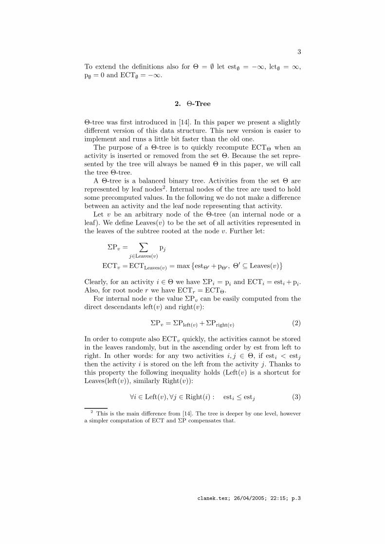
To extend the definitions also for Θ = ∅ let est∅ = −∞, lct∅ = ∞,p∅ = 0 and ECT∅ = −∞.

2. Θ-Tree

Θ-tree was first introduced in [14]. In this paper we present a slightlydifferent version of this data structure. This new version is easier toimplement and runs a little bit faster than the old one.

The purpose of a Θ-tree is to quickly recompute ECTΘ when anactivity is inserted or removed from the set Θ. Because the set repre-sented by the tree will always be named Θ in this paper, we will callthe tree Θ-tree.

A Θ-tree is a balanced binary tree. Activities from the set Θ arerepresented by leaf nodes2. Internal nodes of the tree are used to holdsome precomputed values. In the following we do not make a differencebetween an activity and the leaf node representing that activity.

Let v be an arbitrary node of the Θ-tree (an internal node or aleaf). We define Leaves(v) to be the set of all activities represented inthe leaves of the subtree rooted at the node v. Further let:

ΣPv =∑

j∈Leaves(v)

pj

ECTv =ECTLeaves(v) = max

estΘ′ +pΘ′ , Θ′ ⊆ Leaves(v)

Clearly, for an activity i ∈ Θ we have ΣPi = pi and ECTi = esti +pi.Also, for root node r we have ECTr = ECTΘ.

For internal node v the value ΣPv can be easily computed from thedirect descendants left(v) and right(v):

ΣPv = ΣPleft(v) +ΣPright(v) (2)

In order to compute also ECTv quickly, the activities cannot be storedin the leaves randomly, but in the ascending order by est from left toright. In other words: for any two activities i, j ∈ Θ, if esti < estj

then the activity i is stored on the left from the activity j. Thanks tothis property the following inequality holds (Left(v) is a shortcut forLeaves(left(v)), similarly Right(v)):

∀i ∈ Left(v),∀j ∈ Right(i) : esti ≤ estj (3)

2 This is the main difference from [14]. The tree is deeper by one level, howevera simpler computation of ECT and ΣP compensates that.

clanek.tex; 26/04/2005; 22:15; p.3

4

Proposition 1. For an internal node v, the value ECTv can be com-puted by the following recursive formula:

ECTv = max

ECTright(v), ECTleft(v) +ΣPright(v)

(4)

Proof. From the definition (1), the value ECTv is:

ECTv = ECTLeaves(v) = max

estΘ′ +pΘ′ , Θ′ ⊆ Leaves(v)

With respect to the node v we will split the sets Θ′ into the followingtwo categories:

1. Left(v) ∩ Θ′ = ∅, i.e. Θ′ ⊆ Right(v). Clearly:

max

estΘ′ +pΘ′ , Θ′ ⊆ Right(v)

= ECTRight(v) = ECTright(v)

2. Left(v)∩Θ′ 6= ∅. Then estΘ′ = estΘ′∩Left(v) because of the property(3). Let S be the set of all possible Θ′ considered now:

S = Θ′, Θ′ ⊆ Θ & Θ′ ∩ Left(v) 6= ∅

Thus:

max

estΘ′ +pΘ′ , Θ′ ⊆ S

=

= max

estΘ′∩Left(v) +pΘ′∩Left(v) +pΘ′∩Right(v), Θ′ ⊆ S

=

= max

estΘ′∩Left(v) +pΘ′∩Left(v), Θ′ ⊆ S

+ pRight(v) =

= ECTleft(v) +ΣPright(v)

Therefore the formula (4) is correct. 2

Figure 1 shows an example of a Θ-tree.Thanks to the recursive formulae (2) and (4), the values ECTv and

ΣPv can be easily computed within usual operations with a balanced bi-nary tree without changing their time complexities. Table I summarizestime complexities of different operations with a Θ-tree.

Notice that so far Θ-tree does not require any particular way ofbalancing. The only requirement is a time complexity O(log n) forinserting or deleting a leaf, and time complexity O(1) for finding aroot node.

According to authors experience, the fastest way to implement Θ-tree is to make the shape of the tree fixed during the whole compu-tation. We start with the perfectly balanced tree which represents allactivities on the resource. To indicate that an activity i is not in theset Θ it is enough to set ΣPi = 0 and ECTi = −∞. Clearly, these

clanek.tex; 26/04/2005; 22:15; p.4

5

ΣP = 25

ECT = 45

ΣP = 11

ECT = 31

ΣP = 14

ECT = 44

esta = 0

pa = 5

ΣPa = 5

ECTa = 5

estb = 25

pb = 6

ΣPb = 6

ECTb = 31

estc = 30

pc = 4

ΣPc = 4

ECTc = 34

estd = 32

pd = 10

ΣPd = 10

ECTd = 52

Figure 1. An example of a Θ-tree for Θ = a, b, c, d.

Table I. Time complexities of opera-tions on Θ-tree.

Operation Time Complexity

Θ := ∅ O(1) or O(n log n)

Θ := Θ ∪ i O(log n)

Θ := Θ \ i O(log n)

ECTΘ O(1)

additional “empty” leaves will not interfere with the formulae (2) and(4).

3. Overload checking using Θ-tree

Let us consider an arbitrary set Ω ⊆ T . The overload rule (see e.g. [16])says that if the set Ω cannot be processed within its time bounds thenno solution exists:

∀Ω ⊆ T : (estΩ +pΩ > lctΩ ⇒ fail) (5)

Let us suppose for a while that we are given an activity j ∈ T and wewant to check this rule only for these sets Ω ⊆ T which have lctΩ = lctj .Now in the following consider the set Θ(j):

Θ(j) = k, k ∈ T & lctk ≤ lctj

Overloaded set Ω with lctΩ = lctj exists if and only if ECTΘ(j) > lctj .The idea of the algorithm is to take activities j in ascending order bylctj and adjust the set Θ accordingly.

clanek.tex; 26/04/2005; 22:15; p.5

6

1 Θ := ∅ ;2 for j ∈ T in ascending order of lctj do begin3 Θ := Θ ∪ j ;4 i f ECTΘ > lctj then5 f a i l ; No solution exists6 end ;

Time complexity of this algorithm is O(n log n): the activities haveto be sorted and n-times an activity is inserted into the set Θ.

4. Not-first/not-last using Θ-tree

Not-first and not-last [2], [12] are two symmetric propagation algo-rithms for a unary resource. From these two, we will consider only thenot-last algorithm.

Let us consider a set Ω ⊆ T and an activity i ∈ (T \ Ω). The activityi cannot be scheduled after the set Ω (i.e. i is not last within Ω ∪ i)if:

estΩ +pΩ > lcti −pi (6)

In that case, at least one activity from the set Ω must be scheduledafter the activity i. Therefore the value lcti can be updated:

lcti := min

lcti, max

lctj −pj, j ∈ Ω

(7)

There are two versions of the not-first/not-last algorithms: [2] and[12]. Both of them have time complexity O(n2). The first algorithm [2]finds all the reductions resulting from the previous rules in one pass.Still, after this propagation, next run of the algorithm may find morereductions (not-first and not-last rules are not idempotent). Thereforethe algorithm should be repeated until no more reduction is found (i.e.a fixpoint is reached). The second algorithm [12] is simpler and faster,but more iterations of the algorithm may be needed to reach a fixpoint.

The algorithm presented here may also need more iterations to reacha fixpoint than the algorithm [2] maybe even more than the algorithm[12]. However, time complexity is reduced from O(n2) to O(n log n).

Let us suppose that we have chosen a particular activity i and nowwe want to update lcti according to the not-last rule. To really achievesome changes of lcti using the rule (7), the set Ω must fulfil the followingproperty:

max

lctj −pj , j ∈ Ω

< lcti

clanek.tex; 26/04/2005; 22:15; p.6

7

Therefore:

Ω ⊆

j, j ∈ T & lctj −pj < lcti & j 6= i

We will use the same trick as [12]: because the search for the best

update of lcti may be time consuming we will simply search for some up-date of lcti. If lcti can be updated better, it will be done in subsequentruns of the algorithm. In fact, our algorithm updates lcti to

max

lctj −pj , j ∈ T & lctj −pj < lcti

which is the “smallest” possible update among all possible updates3.Let us define the set Θ(i):

Θ(i) =

j, j ∈ T & lctj −pj < lcti

Thus: lcti can be changed according to the rule not-last if and onlyif there is some set Ω ⊆ (Θ(i) \ i) for which the inequality (6) holds.The only problem is to decide whether such a set Ω exists or not.

Let us recall the definition (1) of ECT and use it on the set Θ(i)\i:

ECTΘ(i)\i = max estΩ +pΩ, Ω ⊆ Θ(i) \ i

Notice, that ECTΘ(i)\i is exactly the maximum value which can be onthe left side of the inequality (6). Therefore there is a set Ω for whichthe inequality (6) holds if and only if:

ECTΘ(i)\i > lcti −pi

The algorithm proceeds as follows. Activities i are taken in the as-cending order of lcti. For each single activity i the set Θ(i) is computedby extending the set Θ(i) of previous activity i4. For each i ECTΘ(i)\i

is checked and lcti is eventually updated:

1 for i ∈ T do2 lct′i := lcti ;3 Θ := ∅ ;4 Q := queue of all activities j ∈ T in ascending order of lctj −pj ;

5 for i ∈ T in ascending order of lcti do begin

3 Notice that the condition i 6= j is not really necessary. If there exists atleast one j 6= i such that lctj −pj < lcti then even in the case lcti − pi =

max

lctj − pj , j ∈ T & lctj − pj < lcti

this value provides legal update of lcti.This property is used at line 13 of the algorithm.

4 Using the simple fact that lctk ≤ lctl implies Θ(k) ⊆ Θ(l), i.e. the Θ(i) sets arenested in the ascending order of lcti.

clanek.tex; 26/04/2005; 22:15; p.7

8

6 while lcti > lctQ.first −pQ.first do begin

9 j := Q. f i r s t ;10 Θ := Θ ∪ j ;11 Q. dequeue ;12 end ;13 i f ECTΘ\i > lcti −pi then

14 lct′i := min

lctj −pj , lct′i

;

15 end ;16 for i ∈ T do17 lcti := lct′i ;

Lines 9–11 are repeated n times maximum over all iterations of thefor cycle on the line 5, because each time an activity is removed fromthe queue. Check on the line 13 can be done in O(log n). Therefore thetime complexity of the algorithm is O(n log n).

Without changing the time complexity, the algorithm can be slightlyimproved: the not-last rule can be also checked for the activity Q.firstjust before the insertion of the activity Q.first into the set Θ (i.e. afterthe line 6):

7 i f ECTΘ > lctQ.first −pQ.first then

8 lct′Q.first := lctj −pj ;

This modification may in some cases save few iterations of thealgorithm.

5. Detectable Precedences

The Figure 2 is taken from [13]. It shows a situation when neitheredge-finding nor the not-first/not-last algorithm can change any timebound, but a propagation of detectable precedences can (see section 6for details on edge-finding algorithm).

A

B

C

pA = 11

pB = 10

pC = 5

0 = estA lctA = 25

1 = estB lctB = 27

estC = 14 lctC = 35

Figure 2. A sample problem for detectable precedences

clanek.tex; 26/04/2005; 22:15; p.8

9

Edge-finding algorithm recognizes that the activity A must be pro-cessed before the activity C, i.e. A C, and similarly B C. Still,each of these precedences alone is weak: they do not enforce any changeof any time bound. However, from the knowledge A,B C we candeduce estC ≥ estA +pA +pB = 21.

A precedence j i is called detectable, if it can be “discovered”only by comparing the time bounds of these two activities:

esti +pi > lctj −pj ⇒ j i (8)

Notice that both precedences A C and B C are detectable.

There is a simple quadratic algorithm, which propagates all knownprecedences on a resource. For each activity i build a set Ω = j ∈T, j i. Note that precedences j i can be of any type: detectableprecedences, search decisions or initial constraints. Using such a set Ω,esti can be adjusted: esti := max esti, ECTΩ because Ω i.

1 for i ∈ T do begin2 m := −∞ ;3 for j ∈ T in non-decreasing order of estj do4 i f j i then5 m := max m, estj + pj ;

6 esti := max m, esti ;7 end ;

A symmetric algorithm adjusts lcti.

However, propagation of only detectable precedences can be donewithin O(n log n). Let Θ(i) be the following set of activities:

Θ(i) =

j, j ∈ T & esti +pi > lctj −pj

Thus Θ(i) \ i is a set of all activities which must be processed beforethe activity i because of detectable precedences. Using the set Θ(i)\ithe value esti can be adjusted:

esti := max

esti, ECTΘ(i)\i

There is also a symmetric rule for precedences j i, but we will notconsider it here, nor the resulting symmetric algorithm.

Our algorithm is based on the observation that set Θ(i) does nothave to be constructed from scratch for each activity i. Rather, theset Θ(i) can be computed incrementally in the similar way as in theprevious section.

clanek.tex; 26/04/2005; 22:15; p.9

10

1 Θ := ∅ ;2 Q := queue of all activities j ∈ T in ascending order of lctj −pj ;

3 for i ∈ T in ascending order of esti +pi do begin4 while esti +pi > lctQ.first −pQ.first do begin

5 Θ := Θ ∪ Q.first ;6 Q. dequeue ;7 end ;

8 est′i := max

esti, ECTΘ\i

;

9 end ;10 for i ∈ T do11 esti := est′i ;

Initial sorts takes O(n log n). Lines 5 and 6 are repeated n timesmaximum over all iterations of the for cycle, because each time anactivity is removed from the queue. Line 8 can be done in O(log n).Therefore the time complexity of the algorithm is O(n log n).

6. Edge-Finding using Θ-Λ-tree

Edge-finding is probably the most often used filtering algorithm for aunary resource constraint. Let us first recall classical edge-finding rules[2]. Consider a set Ω ⊆ T and an activity i 6∈ Ω. If the following con-dition holds, then the activity i has to be scheduled after all activitiesfrom Ω:

∀Ω ⊂ T, ∀i ∈ (T \ Ω) :

estΩ∪i +pΩ∪i = min estΩ, esti + pΩ +pi > lctΩ ⇒ Ω i (9)

Once we know that the activity i must be scheduled after the set Ω,we can adjust esti:

Ω i ⇒ esti := max esti, ECTΩ (10)

Edge-finding algorithm propagates according to this rule and itssymmetric version. There are several implementations of edge-findingalgorithm, two different quadratic algorithms can be found in [11, 3],[6] presents an O(n log n) algorithm.

In the following we present another edge-finding algorithm with timecomplexity O(n log n). It is quite simpler than the algorithm by Carlierand Pinson [6] and it is faster than the quadratic algorithms [11, 3]which are widely used today.

clanek.tex; 26/04/2005; 22:15; p.10

11

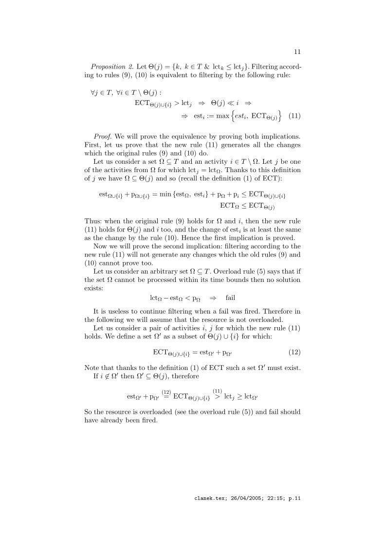
Proposition 2. Let Θ(j) = k, k ∈ T & lctk ≤ lctj. Filtering accord-ing to rules (9), (10) is equivalent to filtering by the following rule:

∀j ∈ T, ∀i ∈ T \ Θ(j) :

ECTΘ(j)∪i > lctj ⇒ Θ(j) i ⇒

⇒ esti := max

esti, ECTΘ(j)

(11)

Proof. We will prove the equivalence by proving both implications.First, let us prove that the new rule (11) generates all the changeswhich the original rules (9) and (10) do.

Let us consider a set Ω ⊆ T and an activity i ∈ T \ Ω. Let j be oneof the activities from Ω for which lctj = lctΩ. Thanks to this definitionof j we have Ω ⊆ Θ(j) and so (recall the definition (1) of ECT):

estΩ∪i +pΩ∪i = min estΩ, esti + pΩ +pi ≤ ECTΘ(j)∪i

ECTΩ ≤ ECTΘ(j)

Thus: when the original rule (9) holds for Ω and i, then the new rule(11) holds for Θ(j) and i too, and the change of esti is at least the sameas the change by the rule (10). Hence the first implication is proved.

Now we will prove the second implication: filtering according to thenew rule (11) will not generate any changes which the old rules (9) and(10) cannot prove too.

Let us consider an arbitrary set Ω ⊆ T . Overload rule (5) says that ifthe set Ω cannot be processed within its time bounds then no solutionexists:

lctΩ − estΩ < pΩ ⇒ fail

It is useless to continue filtering when a fail was fired. Therefore inthe following we will assume that the resource is not overloaded.

Let us consider a pair of activities i, j for which the new rule (11)holds. We define a set Ω′ as a subset of Θ(j) ∪ i for which:

ECTΘ(j)∪i = estΩ′ +pΩ′ (12)

Note that thanks to the definition (1) of ECT such a set Ω′ must exist.If i 6∈ Ω′ then Ω′ ⊆ Θ(j), therefore

estΩ′ +pΩ′

(12)= ECTΘ(j)∪i

(11)> lctj ≥ lctΩ′

So the resource is overloaded (see the overload rule (5)) and fail shouldhave already been fired.

clanek.tex; 26/04/2005; 22:15; p.11

12

Thus i ∈ Ω′. Let us define Ω = Ω′ \ i. We will assume that Ω 6= ∅,because otherwise esti ≥ ECTΘ(j) and rule (11) changes nothing. Forthis set Ω we have:

min estΩ, esti+pΩ +pi = estΩ′ +pΩ′

(12)= ECTΘ(j)∪i

(11)> lctj ≥ lctΩ

Hence the rule (9) holds for the set Ω. To complete the proof we have toshow that both rules (10) and (11) adjust esti equivalently, i.e. ECTΩ =ECTΘ(j). We already know that ECTΩ ≤ ECTΘ(j) because Ω ⊆ Θ(j).Suppose now for a contradiction that

ECTΩ < ECTΘ(j) (13)

Let Φ be a set Φ ⊆ Θ(j) such that:

ECTΘ(j) = estΦ +pΦ (14)

Therefore:

estΩ +pΩ ≤ ECTΩ

(13)< ECTΘ(j)

(14)= estΦ +pΦ (15)

Because the set Ω′ = Ω ∪ i defines the value of ECTΘ(j)∪i (i.e.estΩ′ +pΩ′ = ECTΘ(j)∪i), it has the following property (see the defi-nition (1) of ECT):

∀k ∈ Θ(j) ∪ i : estk ≥ estΩ′ ⇒ k ∈ Ω′

And because Ω = Ω′ \ i:

∀k ∈ Θ(j) : estk ≥ estΩ′ ⇒ k ∈ Ω (16)

Similarly, the set Φ defines the value of ECTΘ(j):

∀k ∈ Θ(j) : estk ≥ estΦ ⇒ k ∈ Φ (17)

Combining properties (16) and (17) together we have that either Ω ⊆ Φ(if estΩ′ ≥ estΦ) or Φ ⊆ Ω (if estΩ′ ≤ estΦ). However, Φ ⊆ Ω is notpossible, because in this case estΦ +pΦ ≤ ECTΩ which contradicts theinequality (15). The result is that Ω ( Φ, and so pΩ < pΦ.

Now we are ready to prove the contradiction:

ECTΘ(j)∪i(12)=

= estΩ′ +pΩ′

= min estΩ, esti + pΩ +pi because Ω = Ω′ \ i

= min estΩ +pΩ +pi, esti +pΩ +pi

< min estΦ +pΦ +pi, esti +pΦ +pi by (15) and pΩ < pΦ

≤ ECTΘ(j)∪i because Φ ⊆ Θ(j)

2

clanek.tex; 26/04/2005; 22:15; p.12

13

Property 1. The rule (11) has a very useful property. Let us consideran activity i and two different activities j1 and j2 for which the rule(11) holds. Moreover let lctj1 ≤ lctj2 . Then Θ(j1) ⊆ Θ(j2) and soECTΘ(j1) ≤ ECTΘ(j2), therefore j2 yields better propagation than j1.Thus for a given activity i it is sufficient to look for the activity j forwhich (11) holds and lctj is maximum.

6.1. Θ-Λ-tree

Let us consider the alternative edge-finding rule (11). We choose anarbitrary activity j and check the rule (11) for each applicable activity i,i.e. we would like to find all activities i for which the following conditionholds:

ECTΘ(j)∪i > lctj

Unfortunately, such an algorithm using Θ-tree would be slow: beforethe check can be performed, each particular activity i must be addedinto the Θ-tree, and after the check the activity i have to be removedback from the Θ-tree.

The idea how to surpass this problem is to extend the Θ-tree struc-ture in the following way: all applicable activities i will be also includedin the tree, but as gray nodes. A gray node represents an activity i whichis not really in the set Θ. However, we are curious what would happenwith ECTΘ if we are allowed to include one of the gray activities intothe set Θ. More exactly: let Λ ⊆ T be a set of all gray activities,Λ ∩ Θ = ∅. The purpose of the Θ-Λ-tree is to compute the followingvalue:

ECT(Θ,Λ) = max(

ECTΘ ∪

ECTΘ∪i, i ∈ Λ)

The meaning of the values ECT and ΣP in the new tree remainsthe same, however only regular (white) nodes are taken into account.Moreover, in order to compute ECT(Θ,Λ) quickly, we add the followingtwo values into each node of the tree:

ΣPv = max

pΘ′ , Θ′ ⊆ Leaves(v) & |Θ′ ∩ Λ| ≤ 1

= max 0 ∪ pi, i ∈ Leaves(v) ∩ Λ +∑

i∈Leaves(v)∩Θ

pi

ECTv = ECTLeaves(v) = max

estΘ′ +pΘ′ , Θ′ ⊆ Leaves(v) & |Θ′ ∩ Λ| ≤ 1

ΣP is maximum sum of processing times of activities in a subtree if oneof gray activities can be used. Similarly ECT is an earliest completiontime of a subtree with at most one gray activity included. For exampleof the Θ-Λ-tree see Figure 3.

clanek.tex; 26/04/2005; 22:15; p.13

14

An idea how to compute values ΣPv and ECTv for internal node v

follows. A gray activity can be used only once: in the left subtree of v

or in the right subtree of v. Note that the gray activity used for ΣPv

can be different from the gray activity used for ECTv. The formulae(2) and (4) can be modified to handle gray nodes:

ΣPv =max

ΣPleft(v) +ΣPright(v), ΣPleft(v) +ΣPright(v)

ECTv =max

ECTright(v), (a)

ECTleft(v) +ΣPright(v), ECTleft(v) +ΣPright(v)

(b)

Line (a) considers all sets Θ′ such that Θ′∩Leaves(left(v)) 6= ∅ (see thedefinition (1) of ECT on page 2). Line (b) considers all sets Θ′ suchthat Θ′ ∩ Leaves(left(v)) 6= ∅.

ΣP = 21

ECT = 44

ΣP = 26

ECT = 49

ΣP = 11

ECT = 34

ΣP = 11

ECT = 34

ΣP = 10

ECT = 42

ΣP = 15

ECT = 45

esta = 0

pa = 5

ΣPa = 5

ECTa = 5

ΣPa = 5

ECTa = 5

estb = 25

pb = 9

ΣPb = 9

ECTb = 34

ΣPb = 9

ECTb = 34

estc = 30

pc = 5

ΣPc = 0

ECTc = −∞

ΣPc = 5

ECTc = 35

estd = 32

pd = 10

ΣPd = 10

ECTd = 42

ΣPd = 10

ECTd = 42

Figure 3. An example of a Θ-Λ-tree for Θ = a, b, d and Λ = c.

Thanks to these recursive formulae, ECT and ΣP can be computedwithin usual operations with balanced binary trees without changingtheir time complexities. Note that together with ECT we can computefor each node v the gray activity which is responsible for ECTk. We needto know such responsible gray activity in the following algorithms.

Table II shows time complexities of selected operations on Θ-Λ-tree.

6.2. Edge-Finding Algorithm

The algorithm starts with Θ = T and Λ = ∅. Activities are sequentially(in descending order by lctj) moved from the set Θ into the set Λ, i.e.

clanek.tex; 26/04/2005; 22:15; p.14

15

Table II. Time complexities of operations onΘ-Λ-tree.

Operation Time Complexity

(Θ, Λ) := (∅, ∅) O(1)

(Θ, Λ) := (T, ∅) O(n log n)

(Θ, Λ) := (Θ \ i, Λ ∪ i) O(log n)

Θ := Θ ∪ i O(log n)

Λ := Λ ∪ i O(log n)

Λ := Λ \ i O(log n)

ECT(Θ, Λ) O(1)

ECTΘ O(1)

white nodes are discolored to gray. As soon as ECT(Θ, Λ) > lctΘ, aresponsible gray activity i is updated. Thanks to the property 1 (page13) the activity i cannot be updated better, therefore we can removethe activity i from the tree (i.e. remove it from the set Λ).

1 for i ∈ T do2 est′i := esti ;3 (Θ, Λ) := (T, ∅) ;4 Q := queue of all activities j ∈ T in descending order of lctj ;5 j := Q.first ;6 repeat7 (Θ, Λ) := (Θ \ j, Λ ∪ j) ;8 Q.dequeue ;9 j := Q.first ;

10 i f ECTΘ > lctj then11 f a i l ; Resource is overloaded

12 while ECT(Θ, Λ) > lctj do begin

13 i := gray activity responsible for ECT(Θ, Λ) ;14 est′i := maxesti, ECTΘ ;15 Λ := Λ \ i ;16 end ;17 until Q.size = 0 ;18 for i ∈ T do19 esti := est′i ;

Note that at line 13 there have to be some gray activity responsiblefor ECT(Θ, Λ) because otherwise we would end up by fail on line 11.

During the entire run of the algorithm, the maximum number ofiterations of the inner while loop is n, because each iteration removes

clanek.tex; 26/04/2005; 22:15; p.15

16

an activity from the set Λ. Similarly, the number of iterations of therepeat loop is n, because each time an activity is removed from thequeue Q. According to Table II time complexity of each single linewithin the loops is O(log n) maximum. Therefore the time complexityof the whole algorithm is O(n log n).

Note that at the beginning Θ = T and Λ = ∅, hence there are nogray activities and therefore ECTk = ECTk and ΣPk = ΣPk for eachnode k. Hence we can save some time by building the initial Θ-Λ-treeas a “normal” Θ-tree.

7. Optional Activities

Nowadays, many practical scheduling problems have to deal with alter-natives – activities which can choose their resource, or activities whichexist only if a particular alternative of processing is chosen. From theresource point of view, it is not yet decided whether such activities willbe processed or not. Therefore we will call such activities optional. Foran optional activity, we would like to speculate what would happen ifthe activity actually would be processed by the resource.

Traditionally, resource constraints are not designed to handle op-tional activities properly. However, several different modifications areused to model them:

Dummy activities. It is basically a workaround for constraint solverswhich do not allow to add more activities on the resource dur-ing problem solving (i.e. resource constraint is not dynamic [4]).Processing times of activities are changed from constants to do-main variables. Several “dummy” activities with possible process-ing times 〈0, ∞) are added on the resource as a reserve for lateractivity addition. Filtering algorithms work as usual, but theyuse minimal possible processing time instead of original constantprocessing time. Note that dummy activities have no influenceon other activities on the resource, because their processing timecan be zero. Once an alternative is chosen, a dummy activity isturned into a regular activity (i.e. minimal processing time is nolonger zero). The main disadvantage of this approach is that animpossibility of a particular alternative cannot be found beforethat alternative is actually tried.

Filtering of options. The idea is to run a filtering algorithm severaltimes, each time with one of the optional activities added on the re-source. When a fail is found, then the optional activity is rejected.Otherwise time bounds of the optional activity can be adjusted.[5] introduces so called PEX-edge-finding with time complexity

clanek.tex; 26/04/2005; 22:15; p.16

17

O(n3). This is a pretty strong propagation, however rather timeconsuming.

Modified filtering algorithms. Regular and optional activities aretreated differently: optional activities do not influence any otheractivity on the resource, however regular activities influence otherregular activities and also optional activities [9]. Most of the fil-tering algorithms can be modified this way without changing theirtime complexities. However, this approach is a little bit weakerthan the previous one, because the previous one also checked whetheraddition of an optional activity would not cause an immediate fail.

Cumulative resources. If we have a set of similar alternative ma-chines, this set can be modeled as a cumulative resource. Thisadditional (redundant) constraint can improve the propagationbefore activities are distributed between the machines. There isalso a special filtering algorithm [16] designed to handle this typeof alternatives.

To handle optional activities we extend each activity i by a variablecalled existencei with the domain true, false. When existencei = truethen i is a regular activity, when existencei ∈ true, false then i isan optional activity. Finally when existence = false we simply excludethis activity from all our considerations.

To make the notation concerning optional activities easy, let R bethe set of all regular activities and O the set of all optional activities.

For optional activities, we would like to consider the following is-sues:

1. If an optional activity should be processed by the resource (i.e. ifan optional activity is changed to a regular activity), would theresource be overloaded? The resource is overloaded if there is sucha set Ω ⊆ R that:

estΩ +pΩ > lctΩ

Certainly, if a resource is overloaded then the problem has nosolution. Hence if an addition of a optional activity i results inoverloading then we can conclude that existencei = false.

2. If the addition of an optional activity i does not result in overload-ing, what is the earliest possible start time and the latest possiblecompletion time of the activity i with respect to regular activitieson the resource? We would like to apply usual filtering algorithmsfor the activity i, however the activity i cannot cause change of anyregular activity.

3. If we add an optional activity i, will the first run of a filtering algo-rithm result in a fail? For example algorithm detectable precedences

clanek.tex; 26/04/2005; 22:15; p.17

18

can increase estk of some activity k so much that estk +pk > lctk.In that case we can also propagate existencei = false.

We will consider the item 1 in the next section “Overload Checking withOptional Activities”. Items 2 and 3 are discussed in section “Filteringwith Optional Activities”.

8. Overload Checking with Optional Activities

In this section we present modified overload checking algorithm whichcan handle optional activities. Basically, the original overload rule (5)remains valid, however we must consider regular activities R only:

∀Ω ⊆ R : (lctΩ − estΩ < pΩ ⇒ fail)

In section 3 we showed that this rule is equivalent with:

∀j ∈ R :(

ECTΘ(j) > lctj ⇒ fail)

(18)

where Θ(j) is:Θ(j) = k, k ∈ R & lctk ≤ lctj

Let us now take into account an optional activity o ∈ O. If processingof this activity would result in overloading, then the activity can neverbe processed by the resource:

∀o ∈ O, ∀Ω ⊆ R :(

estΩ∪o +pΩ∪o > lctΩ∪o ⇒ existenceo := false)

(19)

Let the set Λ(j) be defined in the following way:

Λ(j) = o, o ∈ O & lcto ≤ lctj

The rule (19) is applicable if and only if there is such an activity j ∈ T

such that ECT(Θ(j),Λ(j)) > lctj . In this case, the activity which isresponsible for ECT(Θ(j),Λ(j)) can be excluded from the resource.

The following algorithm detects overloading, it also deletes all op-tional activities k such that an addition of this activity k alone causesan overload. Of course, a combination of several optional activities maystill cause an overload.

1 (Θ, Λ) := (∅, ∅) ;

2 for i ∈ T in ascending order5 of lcti do begin

5 In case of ties optional activities should be taken before regular activities.

clanek.tex; 26/04/2005; 22:15; p.18

19

3 i f i is a optional activity then4 Λ := Λ ∪ i ;5 else begin6 Θ := Θ ∪ i ;7 i f ECTΘ > lcti then8 f a i l ; No solution exists

9 while ECT(Θ, Λ) > lcti do begin

10 k := optional activity responsible for ECT(Θ, Λ) ;11 existencek := false ;12 Λ := Λ \ k ;13 end ;14 end ;15 end ;

The time complexity of the algorithm is again O(n log n). The innerwhile loop is repeated n times maximum because each time an activityis removed from the set Λ. The outer for loop has also n iterations,time complexity of each single line is O(log n) maximum (see the TableII).

9. Filtering with Optional Activities

The following section is an example of how to extend a certain classof filtering algorithms to handle optional activities. The idea is simple:if the original algorithm uses Θ-tree, the modified algorithm uses Θ-Λ-tree instead. Optional activities are represented by gray nodes ofthe tree. For regular propagation, value ECTΘ is used the same wayas before. However, also ECT(Θ,Λ) is used now: if propagation usingECT(Θ,Λ) would result in an immediate fail then the optional activityresponsible for that is excluded from the resource.

Let us demonstrate this idea on the detectable precedences algo-rithm:

1 (Θ,Λ) := (∅, ∅) ;2 Q := queue of all activities j ∈ T in ascending order of lctj −pj ;

3 for i ∈ T in ascending order of esti +pi do begin4 while esti +pi > lctQ.first −pQ.first do begin

5 i f i is a regular activity then6 Θ := Θ ∪ Q.first ;7 else8 Λ := Λ ∪ Q.first ;9 Q. dequeue ;

10 end ;

clanek.tex; 26/04/2005; 22:15; p.19

20

11 est′i := max

esti, ECTΘ\i

;

12 i f i is a regular activity then

13 while ECT(Θ \ i ,Λ) > lcti −pi then begin

14 k := an optional activity responsible for ECT (Θ \ i ,Λ) ;15 Λ := Λ \ k ;16 existencek := false ;17 end ;18 end ;19 for i ∈ T do20 esti := est′i ;

Optional activities are stored in the set Λ, therefore they are nottaken into account when the new value est′i is computed at the line 11.

At line 13 there is a check what would happen if one of the optionalactivities become regular one. In that case est′i would be ECT(Θ \ i ,Λ).If est′i > lcti −pi then the activity k can be excluded from the resource.

The complexity of the algorithm remains the same: O(n log n).

The same idea can be used to extend the not-first/not-last algo-rithm:

1 for i ∈ T do2 lct′i := lcti ;3 (Θ,Λ) := (∅, ∅) ;4 Q := queue of all activities j ∈ T in ascending order of lctj −pj ;

5 for i ∈ T in ascending order of lcti do begin6 while lcti > lctQ.first −pQ.first do begin

9 j′ := Q. f i r s t ;10 i f j′ is regular activity then begin11 j := j′ ;12 Θ := Θ ∪ j ;13 end else begin14 Λ := Λ ∪ j ′ ;15 end ;16 Q. dequeue ;17 end ;18 i f ECTΘ\i > lcti −pi then

19 lct′i := min

lctj −pj , lct′i

;

20 i f i is regular activity and lctj′ −pj′ < esti +pi then

21 while ECT(Θ \ i ,Λ) > lcti −pi do begin

22 k := an optional activity responsible for ECT (Θ \ i ,Λ) ;23 Λ := Λ \ k ;24 existencek := false ;

clanek.tex; 26/04/2005; 22:15; p.20

21

25 end ;26 end ;27 for i ∈ T do28 lcti := lct′i ;

Again, optional activities are stored in the gray nodes of the Θ-Λ-tree, therefore they do not influence new time bound lct′i computed atthe line 20. At the line 25 we are allowed to set existencek := false,because at this point we know that if the activity k become regular,then the propagation would take place (compare lines 22 and 19), how-ever such propagation would result in fail (because lct′i = lctj′ −pj′ <

esti +pi, see line 21). Time complexity of this algorithm is O(n log n).

Unfortunately, extending the edge-finding algorithm is not so easybecause this algorithm already uses Θ-Λ-tree. We will consider this inour future work.

10. Experimental Results

First, we tested our propagation algorithms without optional activi-ties on several jobshop problems taken from the OR library [1]. Thebenchmark problem is to compute a destructive lower bound using theshaving technique [11]. The destructive lower bound is the minimalmakespan for which propagation alone is not able to find conflict with-out backtracking. Shaving is similar to the proof by a contradiction. Wechoose an activity i, limit its esti or lcti and propagate. If an infeasibilityis found, then the limitation was invalid and so we can decrease lcti

or increase esti. To limit CPU time, shaving was used for each activityonly once. For more details about shaving see [11].

Table III shows the results. We measured the CPU6 time in secondsneeded to prove the lower bound. The propagation was done twice:with the upper bounds LB and LB-1. Column T1 shows total runningtime when presented O(n log n) filtering algorithms are used (overloadchecking, detectable precedences, not-first/not-last and edge-finding).Column T2 shows total running times when quadratic algorithms areused: quadratic overload checking, not-first/not-last from [12], edge-finding from [3] and O(n log n) detectable precedences.

As can be seen, the new algorithms are strictly faster and the speedupis increasing with a growing number of jobs.

Optional activities were tested on modified 10x10 jobshop instances.In each job, activities on 5th and 6th place were taken as alternatives.

6 Benchmarks were performed on Intel Pentium Centrino 1300MHz

clanek.tex; 26/04/2005; 22:15; p.21

22

Table III. Destructive Lower Bounds

Prob. Size LB T1 T2

abz5 10 x 10 1196 1.363 1.696

abz6 10 x 10 941 1.717 2.156

ft10 10 x 10 911 1.530 1.949

orb01 10 x 10 1017 1.649 2.123

orb02 10 x 10 869 1.415 1.796

la21 15 x 10 1033 0.691 1.030

la22 15 x 10 925 3.230 4.902

la36 15 x 15 1267 5.012 7.854

la37 15 x 15 1397 2.369 3.584

ta01 15 x 15 1224 8.641 13.66

ta02 15 x 15 1210 6.618 10.41

la26 20 x 10 1218 0.597 1.030

la27 20 x 10 1235 0.745 1.260

la29 20 x 10 1119 2.949 4.954

abz7 20 x 15 651 2.973 4.967

abz8 20 x 15 621 10.71 18.36

ta11 20 x 15 1295 13.24 23.26

ta12 20 x 15 1336 15.64 26.60

ta21 20 x 20 1546 34.98 61.63

ta22 20 x 20 1501 23.06 40.83

yn1 20 x 20 816 24.35 42.70

yn2 20 x 20 842 20.77 36.19

ta31 30 x 15 1764 3.397 7.901

ta32 30 x 15 1774 4.829 11.64

swv11 50 x 10 2983 12.02 39.24

swv12 50 x 10 2972 15.43 46.32

ta51 50 x 15 2760 7.695 26.14

ta52 50 x 15 2756 8.056 27.37

ta71 100 x 20 5464 72.07 432.5

ta72 100 x 20 5181 72.15 432.1

Therefore in each problem there are 20 optional activities and 80 reg-ular activities, resultant schedule has 90 activities. Table IV shows theresults. Column LB is the destructive lower bound computed withoutshaving, column Opt is the optimal makespan. Column CH is the num-ber of choicepoints needed to find the optimal solution and prove the

clanek.tex; 26/04/2005; 22:15; p.22

23

optimality (i.e. optimal makespan used as the initial upper bound).Finally the column T is the CPU time in seconds.

As can be seen in the table, propagation is strong, all of the problemswere solved surprisingly quickly. However more experiments should bemade, especially on real life problem instances.

Table IV. Alternative activities

Prob. Size LB Opt CH T

abz5-alt 10 x 10 1031 1093 283 0.336

abz6-alt 10 x 10 791 822 17 0.026

orb01-alt 10 x 10 894 947 9784 12.776

orb02-alt 10 x 10 708 747 284 0.328

ft10-alt 10 x 10 780 839 4814 6.298

la16-alt 10 x 10 838 842 27 0.022

la17-alt 10 x 10 673 676 24 0.021

la18-alt 10 x 10 743 750 179 0.200

la19-alt 10 x 10 686 731 84 0.103

la20-alt 10 x 10 809 809 14 0.014

11. Conclusions

In this paper we describe new O(n log n) implementations of over-load checking and of several filtering algorithms for the unary resourceconstraint: not-first/not-last, detectable precedences, and edge-finding.The key concepts in these implementations are two novel data struc-tures: Θ-tree and Θ-Λ-tree. These new data structures facilitate adesign of O(n log n) algorithms which are considerably simpler thanthe existing O(n log n) algorithms. This simplicity makes the new algo-rithms relatively easy to implement. Thus they constitute an appealingoption for the replacement of the simple O(n2) algorithms which arecurrently widely used in practice.

Another asset of the presented algorithms (with the exception ofedge- finding) is their modifiability to deal with a set of optional activ-ities. This property is very important for modeling frequently appearingreal-life problems which involve alternative processing of different ac-tivities. Appropriate modifications of all presented filtering algorithms(with the exception of edge-finding) which are able to deal with optionalactivities are described in detail.

clanek.tex; 26/04/2005; 22:15; p.23

24

Future work may go in three different directions. First of all it wouldbe interesting to see, whether also the edge-finding algorithm, whichalready uses the Θ-Λ-tree in the version with no optional activities,can be extended to be able to deal with optional activities. Secondly, itmay be worth investigating whether the tools designed here (mainly thenew data structures) are applicable also elsewhere (of course, this is arather broad and vaguely defined direction). Finally, more experimentscould be run to get a better picture of the performance of the newlyimplemented algorithms.

11.0.1. Acknowledgements:

This work has been supported by the Czech Science Foundation underthe contract no. 201/04/1102.

We would like to thank our referees for taking the time to provideexcellent feedback and critical comment.

References

1. ‘OR Library’. http://mscmga.ms.ic.ac.uk/info.html.2. Baptiste, P. and C. Le Pape: 1996, ‘Edge-Finding Constraint Propagation

Algorithms for Disjunctive and Cumulative Scheduling’. In: Proceedings ofthe Fifteenth Workshop of the U.K. Planning Special Interest Group.

3. Baptiste, P., C. Le Pape, and W. Nuijten: 2001, Constraint-Based Scheduling:Applying Constraint Programming to Scheduling Problems. Kluwer AcademicPublishers.

4. Bartak, R.: 2003, ‘Dynamic Global Constraints in Backtracking Based Envi-ronments’. Annals of Operations Research 118, 101–118.

5. Beck, J. C. and M. S. Fox: 1999, ‘Scheduling Alternative Activities’. In:AAAI/IAAI. pp. 680–687.

6. Carlier, J. and E. Pinson: 1994, ‘Adjustments of Head and Tails for the Job-Shop Problem’. European Journal of Operational Research 78, 146–161.

7. Caseau, Y. and F. Laburthe: 1994, ‘Improved CLP Scheduling with Task In-tervals’. In: P. van Hentenryck (ed.): Proceedings of the 11th InternationalConference on Logic Programming, ICLP’94.

8. Colombani, Y.: 1996, ‘CP: an efficient and partical approach to solving thejob-shop problem’. In: Principles and Practice of Constraint Programming -CP 1996.

9. Focacci, F., P. Laborie, and W. Nuijten: 2000, ‘Solving scheduling prob-lems with setup times and alternative resources’. In: Proceedings of the 5thInternational Conference on Artificial Intelligence Planning and Scheduling.

10. Garey, M. R. and D. S. Johnson: 1979, Computers and Intractability: AGuide to the Theory of NP-Completeness. W.H.Freeman and Company, SanFrancisco.

11. Martin, P. and D. B. Shmoys: 1996, ‘A New Approach to Computing OptimalSchedules for the Job-Shop Scheduling Problem’. In: W. H. Cunningham,S. T. McCormick, and M. Queyranne (eds.): Proceedings of the 5th Interna-

clanek.tex; 26/04/2005; 22:15; p.24

25

tional Conference on Integer Programming and Combinatorial Optimization,IPCO’96. Vancouver, British Columbia, Canada, pp. 389–403.

12. Torres, P. and P. Lopez: 1999, ‘On Not-First/Not-Last conditions in disjunctivescheduling’. European Journal of Operational Research.

13. Vilım, P.: 2002, ‘Batch Processing with Sequence Dependent Setup Times: NewResults’. In: Proceedings of the 4th Workshop of Constraint Programming forDecision and Control, CPDC’02. Gliwice, Poland.

14. Vilım, P.: 2004, ‘O(n log n) Filtering Algorithms for Unary Resource Con-straint’. In: Proceedings of CP-AI-OR 2004.

15. Wolf, A.: 2003, ‘Pruning while Sweeping over Task Intervals’. In: Principlesand Practice of Constraint Programming - CP 2003. Kinsale, Ireland.

16. Wolf, A. and H. Schlenker: 2004, ‘Realizing the Alternative Resources Con-straint Problem with Single Resource Constraints’. In: To appear in proceedingsof the INAP workshop 2004.

clanek.tex; 26/04/2005; 22:15; p.25