Extensible Lattice Sequences for Quasi-Monte Carlo Quadrature

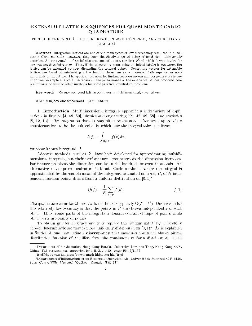
EXTENSIBLE LATTICE SEQUENCES FOR QUASI-MONTE CARLOQUADRATUREFRED J. HICKERNELLyz, HEE SUN HONGy, PIERRE L'�ECUYERx, AND CHRISTIANELEMIEUXxAbstract. Integration lattices are one of the main types of low discrepancy sets used in quasi-Monte Carlo methods. However, they have the disadvantage of being of �xed size. This articledescribes the construction of an in�nite sequence of points, the �rst bm of which form a lattice forany non-negative integer m. Thus, if the quadrature error using an initial lattice is too large, thelattice can be extended without discarding the original points. Generating vectors for extensiblelattices are found by minimizing a loss function based on some measure of discrepancy, or non-uniformity of the lattice. The spectral test used for �nding pseudo-random number generators is oneimportant example of such a discrepancy. The performance of the extensible lattices proposed hereis compared to that of other methods for some practical quadrature problems.Key words. Discrepancy, good lattice point sets, multidimensional, spectral testAMS subject classi�cations. 65D30, 65D321. Introduction. Multidimensional integrals appear in a wide variety of appli-cations in �nance [4, 48, 50], physics and engineering [29, 42, 49, 58], and statistics[8, 12, 13]. The integration domain may often be assumed, after some appropriatetransformation, to be the unit cube, in which case the integral takes the form:I(f) � Z[0;1)s f(x) dxfor some known integrand, f .Adaptive methods, such as [2], have been developed for approximating multidi-mensional integrals, but their performance deteriorates as the dimension increases.For �nance problems the dimension can be in the hundreds or even thousands. Analternative to adaptive quadrature is Monte Carlo methods, where the integral isapproximated by the sample mean of the integrand evaluated on a set, P , of N inde-pendent random points drawn from a uniform distribution on [0; 1)s:Q(f) � 1N Xz2P f(z): (1.1)The quadrature error for Monte Carlo methods is typically O(N�1=2). One reason forthis relatively low accuracy is that the points in P are chosen independently of eachother. Thus, some parts of the integration domain contain clumps of points whileother parts are empty of points.To obtain greater accuracy one may replace the random set P by a carefullychosen deterministic set that is more uniformly distributed on [0; 1)s. As is explainedin Section 3, one may de�ne a discrepancy that measures how much the empiricaldistribution function of P di�ers from the continuous uniform distribution. ThenyDepartment of Mathematics, Hong Kong Baptist University, Kowloon Tong, Hong Kong SAR,China. This research was supported by a HKBU FRG grant 96-97/[email protected], http://www.math.hkbu.edu.hk/~fredxD�epartement d'Informatique et de Recherche Op�erationnelle, Universit�e de Montr�eal C.P. 6128,Succ. Centre-Ville, Montr�eal (Qu�ebec), Canada, H3C 3J71

2 F. J. Hickernell, H. S. Hong, P. L'�Ecuyer and C. Lemieux.one chooses P in quadrature rule (1.1) to have as small a discrepancy as possible.The quadrature methods based on low discrepancy sets are called quasi-Monte Carlomethods. They are discussed in several review articles [3, 16, 40, 59] and monographs[27, 44, 53].Two important families of low discrepancy sets are:i. integration lattices [44, Chap. 5] and [53], andii. digital nets and sequences [44, Chap. 4].These two families are introduced in Section 2. One advantage of the second familyis that any number of consecutive points from a good digital sequence has low dis-crepancy. If one needs more points, one may use additional terms from the digitalsequence without discarding the original ones. On the other hand, until now, thenumber of points in an integration lattice has had to be speci�ed in advance. So far,there has been no systematic way of adding points to an integration lattice while stillretaining its lattice structure.The purpose of this article is to provide a method for constructing in�nite latticesequences, thereby eliminating the need to know N , the number of points, in advance.Although the emphasis is on rank-1 lattices, the method may be applied to integrationlattices of arbitrary rank. Given an in�nite lattice sequence one may approximate amultidimensional integrand with a quadrature rule of the form (1.1) for moderatenumber of points N0. If the error estimate is unacceptably high, then one may choosean additional N1 �N0 points from the lattice sequence to obtain a quadrature rulewith N1 points, and so on.The following section describes the new method for obtaining in�nite lattice se-quences. Section 3 brie y reviews some results on discrepancy and quadrature erroranalysis for quasi-Monte Carlo methods. These are used to �nd the generating vectorsfor the new lattice sequences in Section 4. The issue of error estimation is addressedin Section 5. Two practical examples are explored in Section 6, where the new latticesequences are compared with existing quadrature methods. The last section containssome concluding remarks.2. Integration Lattices and Digital Sequences. This section begins by in-troducing integration lattices. Next, digital sequences and (t; s)-sequences are de-scribed. Finally, the idea underlying digital sequences is used to produce in�nitelattice sequences.2.1. Integration Lattices. Rank-1 lattices, also known as good lattice point(glp) sets, were introduced by Korobov [31] and have been widely studied since then(see [27, 44, 53] and the references therein). The formula for a shifted rank-1 latticeset is simply P = ffih=N +�g : i = 0; : : : ; N � 1g ; (2.1)where N is the number of points, h is an s-dimensional generating vector of integers(a good lattice point) that depends on N , � is an s-dimensional shift vector in [0; 1)s,and fxg denotes the fractional part of a vector x, i.e. fxg = x mod 1. Sloan [52, 54]later generalized glp sets by introducing more than one generating vector. A shiftedintegration lattice withN = N1 � � �Np points based on generating vectors h(1); : : : ; h(p)is:P = nfi1h(1)=N1 + � � �+ iph(p)=Np +�g : ik = 0; : : : ; Nk � 1; k = 1; : : : ; po :Integration lattices and their use for quadrature are discussed in the monograph [53].

Extensible Lattice Sequences 3For a given N there is the problem of choosing good generating vectors. Althoughtheoretical constructions exist for s = 1 and 2, in higher dimensions one typically �ndsgenerating vectors by minimizing a discrepancy or measure of non-uniformity of thelattice. Several examples of discrepancies are given in Section 3.2.2. Digital Nets and Sequences. Digital nets and sequences are anothermethod of constructing low discrepancy sets (see [32] and [44, Chapter 4]). Let bdenote a positive integer greater than one. For any non-negative integer one mayextract the digits of its base b representation, i1; i2; : : : 2 f0; : : : ; b� 1g, only �nitelymany of which are nonzero:i = : : : i3i2i1 (base b) = i1 + i2b+ i3b2 + � � � : (2.2a)The ith term of a digital net or sequence is given byz(i) = (z(i)1 ; : : : ; z(i)s ); (2.2b)z(i)j = 0:�(i)j1 �(i)j2 : : : (base b) = �(i)j1 b�1 + �(i)j2 b�2 + � � � (2.2c)where 0BB@�(i)j1�(i)j2... 1CCA = [email protected] mod b; j = 1; : : : ; s: (2.2d)If the generating matrices C1; : : : ;Cs are m � m, then this construction yields adigital net fz(i) : i = 0; : : : ; bm � 1g with bm points. If the generating matrices are1�1, i.e. each Cj has entries cjkl de�ned for k; l = 1; 2 : : : , then one has a digitalsequence fz(i) : i = 0; 1; : : :g.The prototype digital sequence is the one-dimensional Van der Corput sequence,f�b(i) : i = 0; 1; : : :g. This is de�ned by taking s = 1 and C1 equal to the identitymatrix: �b(i) = 0:i1i2 : : : (base b) = i1b�1 + i2b�2 + : : : : (2.3)In essence, the Van der Corput sequence, takes the b-ary representation of an integerand re ects it about the decimal point.2.3. (t;m; s)-Nets and (t; s)-Sequences. Similarly to integration lattices onehas the problem of how to choose the generating matrices Cj in (2.2). Usually thisis done to optimize the quality factor of the net or sequence. For any non-negatives-vector k, and for a base b consider the following set of disjoint boxes, whose unionis the unit cube:Bk = f[n1b�k1 ; (n1 + 1)b�k1)� � � � � [nsb�ks ; (ns + 1)b�ks): nj = 0; : : : ; bkj � 1g: (2.4)Each such box in Bk has volume b�k1�����ks . A (t;m; s)-net in base b is a set ofN = bm points in [0; 1)s, such that every box in Bk contains bm�k1�����ks of thesepoints for any k satisfying m� k1�� � � � ks � t. Thus, any function that is piecewise

4 F. J. Hickernell, H. S. Hong, P. L'�Ecuyer and C. Lemieux.constant on the boxes in Bk will be integrated exactly according to quadrature rule(1.1) if k1 + � � �+ ks � m� t: (2.5)The integer parameter t is called the quality parameter of the net and it takes valuesbetween 0 and m. A smaller value of t means a better net.A (t; s)-sequence is an in�nite sequence of points in [0; 1)s such that the bm pointsnumbered lbm to (l+1)bm�1 always form a (t;m; s)-net for any non-negative integerl. By using a (t; s)-sequence to do quasi-Monte Carlo calculations, one need not knowthe number of points required in advance. If the �rst bm1 points do not give su�cientaccuracy, then one may add the next bm2 � bm1 points in the sequence to get a netwith bm2 points, without throwing away the �rst bm1 points.There is a connection between digital nets and sequences as de�ned above and(t;m; s)-nets and (t; s)-sequences [32]. Let c(m)ji� denote the vector containing the �rstm elements of the ith row of the the generating matrix Cj . Given a non-negativeinteger s-vector k, let C(m; k) be the following set of the �rst kj rows of the jthgenerating matrix for j = 1; : : : ; s:C(m; k) = nc(m)ji� : i = 1; : : : ; kj ;o :Furthermore, letT (m; s) = mint ft : C(m; k) is a linearly independent set of vectorsfor all k with k1 + � � �+ ks = m� tg;T (s) = maxm T (m; s):The following theorem (see [32]) gives the condition for which a digital net is a (t;m; s)-net and a digital sequence is a (t; s)-sequence.Theorem 2.1. For prime bases b the digital net de�ned above in (2.2) is a(T (m; s);m; s)-net. If, in addition, T (s) is �nite, then the digital sequence de�ned in(2.2) is a (T (s); s)-sequence.Finding good generating matrices for digital nets and sequences is an active areaof research. Virtually all generators found so far have been based on number theoreticarguments. Early sequences include those of Sobol' [56], Faure [9] and Niederreiter[43]. Algorithms for these sequences can be found in the ACM Transactions on Mathe-matical Software collection. The FINDER software developed at Columbia Universityby Traub and Papageorgiou implements generalized Sobol' and generalized Faure se-quences. New constructions with smaller t values are given by Niederreiter and Xing[47].2.4. In�nite Lattice Sequences. The idea underlying digital sequences maybe extended to integration lattices to obtain in�nite lattice sequences. The ith termof a rank-1 lattice, which is fih=Ng, depends inherently on the number of points, N .Thus, the formula for a lattice must be rewritten in a way that does not involve Nexplicitly. A way to do this was �rst suggested in [24].Suppose that the number of points, N , is some integer power of a base b � 2,that is, N = bm. This is the same assumption as for a digital or (t;m; s)-net. The�rst N values of the Van der Corput sequence, de�ned in (2.3) are0bm ; : : : ; bm � 1bm ;

Extensible Lattice Sequences 5although in a di�erent order. Therefore, the term i=N = i=bm; i = 0; : : : ; N � 1, thatappears in the de�nition of the rank-1 lattice may be replaced by �b(i), a term thatdoes not depend on N .The s-dimensional generating vector h in (2.1) typically depends on N also. Itmay be expressed in b-ary form as:h = (h1m : : : h11; h2m : : : h21; : : : ; hsm : : : hs1) (base b);where hjk 2 f0; : : : ; b � 1g are digits. For k > m the digits hjk do not a�ect thede�nition of the rank-1 lattice set with N = bm points since they only contributeintegers to the product �b(i)h. Therefore, each component of h may be written (inprinciple) as an in�nite string of digits:h = (: : : h12h11; : : : h22h21; : : : ; : : : hs2hs1) (base b): (2.6)This single \in�nite" generating vector may serve for all possible values of m.The preceding paragraphs provide the basis for de�ning an in�nite rank-1 latticesequence. Altering the original de�nition in (2.1) leads to the following:Definition 2.2. An in�nite rank-1 lattice sequence in base b with generatingvector h of the form (2.6) and shift � is de�ned as:ff�b(i)h+�g : i = 0; 1; 2; : : :g : (2.7)The �rst bm terms of the in�nite rank-1 lattice sequence (2.7) are a rank-1 lattice.Moreover, just as certain subsets of a (t; s)-sequence are (t;m; s)-nets, so subsets ofan in�nite rank-1 lattice sequence are shifted rank-1 lattices.Theorem 2.3. Suppose that P is the set consisting of the l+1st run of bm termsof the in�nite lattice rank-1 sequence de�ned in (2.7):P = ff�b(lbm + i)h+�g : i = 0; : : : ; bm � 1g ; l = 0; 1; : : : :Then, P is a rank-1 lattice with shift �b(l)b�mh+�, that is,P = �f�b(i)h+ �b(l)b�mh+�g : i = 0; : : : ; bm � 1 :Proof. The proof follows directly from the de�nition of the Van der Corputsequence. For all i = 0; : : : ; bm � 1, note that�b(lbm + i) = �b(i) + �b(lbm) = �b(i) + �b(l)b�m:Substituting the right hand side into the de�nition of P completes the proof.The de�nition of an in�nite rank-1 lattice sequence may be extended to integrationlattices of arbitrary rank.Definition 2.4. An in�nite lattice sequence (of arbitrary rank) with basesb1; : : : ; bp and generating vectors h(1); : : : ; h(p) of the form (2.6) is de�ned as:nf�b1(i1)h(1) + � � �+ �bp(ip)h(p) +�g : i1; : : : ; ip = 0; 1; 2; : : :o (2.8)A practical complication for an integration lattice of rank greater than 1 is that thereare multiple indices, ik, each of which may or may not tend to in�nity, and each at itsown rate. Because of this complication we will focus on rank-1 lattices in the sectionsthat follow. Theorem 2.3 also has a natural extension to in�nite lattice sequences ofarbitrary rank, and its proof is similar.

6 F. J. Hickernell, H. S. Hong, P. L'�Ecuyer and C. Lemieux.3. Discrepancy. Unlike (t; s)-nets for which there exist explicit constructionsof the generating matrices Cj , there are no such explicit constructions of generatingvectors h for rank-1 lattices for arbitrary s. Tables of generating vectors for latticesthat do exist (see [8, 14, 27]) are usually obtained by minimizing some measure ofnon-uniformity, or discrepancy, of the lattice. This section describes several usefuldiscrepancy measures.Let Err(f ;P ) denote the quadrature error for a rule of the form (1.1) for anarbitrary set P . Worst case error analysis of the quadrature error leads to a Koksma-Hlawka-type inequality of the form [23]:jErr(f ;P )j � jI(f)�Q(f)j � D(P )V (f); (3.1)where D(P ) is the discrepancy or measure of nonuniformity of the point set de�ningthe quadrature rule, and V (f) is the variation or uctuation of the integrand, f . Theprecise de�nitions of the discrepancy and the variation depend on the particular spaceof integrands.In the traditional Koksma-Hlawka inequality (see [26] and [44, Theorem 2.11]),the variation is the variation in the sense of Hardy and Krause, and the discrepancyis the L1-star discrepancy:D�(P ) = kFunif(x)� FP (x)k1 = x1 : : : xs � jP \ [0; x]jN 1 : (3.2)Here Funif is the uniform distribution on the unit cube, FP is the empirical distributionfunction for the sample P , and j�j denotes the number of points in a set. The notationk�kp denotes the Lp-norm or the `p-norm, depending on the context. Error bounds ofthe form (3.1) involving the Lp-star discrepancy have been derived by [57, 62]. Errorbounds involving generalizations of the star discrepancy appear in [21, 22, 23, 55].When the integrands belong to a reproducing kernel Hilbert space, the errorbound (3.1) may be easily obtained [21, 23]. The discrepancy may be written interms of the reproducing kernelD(P ) = (Z[0;1)2s K(x; y) d(Funif � FP )(x) d(Funif � FP )(y))1=2 (3.3)= 8<:Z[0;1)2s K(x; y) dx dy � 2N Xz2P Z[0;1)s K(z; y) dy + 1N2 Xz;t2P K(z; t)9=;1=2 :For example, the L2-star discrepancy, whose formula was originally derived in [60], is aspecial case of the above formula withK(x; y) =Qsj=1[1�max(x; y)]. An advantage ofconsidering reproducing kernel Hilbert spaces of integrands is that the computationalcomplexity of the discrepancy is relatively small (at worst O(N2) operations). Bycontrast the L1-star discrepancy requires O(Ns) operations to evaluate.The discrepancy of type (3.3) can also be interpreted as an average-case quadra-ture error [25, 41, 61]. Suppose that the integrand is a random function lying in thesample space A, and suppose that the integrand has zero mean and covariance kernel,K(x; y), that is,Ef2A[f(x)] = 0 and Ef2A[f(x)f(y)] = K(x; y) 8x; y 2 [0; 1)s:

Extensible Lattice Sequences 7Then the root mean square quadrature error over A is the discrepancy as de�ned in(3.3): qEf2A[Err(f ;P )]2 =qEf2A jI(f)�Q(f)j2 = D(P ): (3.4)If P is a simple random sample, then the mean square discrepancy is [25]:EP f[D(P )]2g = 1N (Z[0;1)s K(x; x) dx� Z[0;1)s�[0;1)s K(x; y) dy dx) (3.5)This formula serves as a benchmark for other (presumably superior) low discrepancysets. Since the mean square discrepancy is O(N�1), the discrepancy itself is typicallyO(N�1=2) for a simple random sample. The variance of a function, f , may be de�nedas Var(f) � Z[0;1)s f2 dx� Z[0;1)s f dx!2 :The mean value of the variance over the space of average-case integrands can be shownto be [25]: Ef2A[Var(f)] = Z[0;1)s K(x; x) dx � Z[0;1)2s K(x; y) dy dx; (3.6)which is just the term in braces in (3.5).It may seem odd at �rst that the discrepancy can serve both as an average-caseand worst-case quadrature error. The explanation is that the space of integrands, A,in the average-case analysis is much larger than the space of integrands, W , in theworst-case analysis. See [21, 25] and the references therein for the proofs of the aboveresults as well as further details.There are some known asymptotic results for the discrepancies of (t;m; s)-nets.The L1-star discrepancy of any (t;m; s)-net is O(N�1[logN ]s�1) [44, Theorem 4.10].Moreover, the typical (in the sense of an average taken over all possible nets) L2-star discrepancy of (0;m; s)-nets is O(N�1[logN ](s�1)=2) [19] | the best possible forany set. For discrepancies of the form (3.3) with su�ciently smooth kernels, typical(0;m; s)-nets have O(N�3=2[logN ](s�1)=2) discrepancy [25].Lattice rules, the topic of this article, are known to be particularly e�ective for in-tegrating periodic functions. Suppose that the integrand has an absolutely convergentFourier series with Fourier coe�cients f̂(k):f(x) = Xk2Zs f̂(k)e2�ik0x; f̂(k) = Z[0;1)s f(x)e�2�ik0x dx: (3.7)Here k0x denotes the dot product of the s-dimensional wavenumber vector k with x.The quadrature error for a particular integrand with an absolutely convergentFourier series is simply the sum of the quadrature errors of each term:Err(f ;P ) = � Xk2Zsk 6=0 f̂(k)" 1N Xz2P e2�ik0z# ;

8 F. J. Hickernell, H. S. Hong, P. L'�Ecuyer and C. Lemieux.where the term corresponding to k = 0 does not enter because constants are integratedexactly. One can multiply and divide by arbitrary weights w(k) inside this sum. Thenby applying H�older's inequality one has the following error bound of the form (3.1)[23]: jErr(f ;P )j � DF;p(P )VF;q(f); 1p + 1q = 1; (3.8a)DF;p(P ) = 1fk 6=0gw(k) " 1N Xz2P e2�ik0z#!k2Zs p ; (3.8b)VF;q(f) = �1fk 6=0gw(k)f̂(k)�k2Zs q : (3.8c)Here 1f�g denotes the indicator function. In order to insure that the discrepancy is�nite we assume that the weights increase su�ciently fast as k tends to in�nity: � 1w(k)�k2Zs p <1:If P is the node set of an integration lattice, then it is known that trigonometricpolynomials are integrated exactly for all nonzero wavenumbers not in the dual lattice,L?, (see [53, Lemma 2.7]): 1N Xz2P e2�ik0z = 1fk2L?g:The dual lattice is the set of all k satisfying k0z = 0 (mod 1) 8z 2 P . Thus, for nodesets of lattices the de�nition of discrepancy above may be simpli�ed toDF;p(P ) = �1f06=k2L?gw(k) �k2Zs p :Certain explicit choices of w(k) have appeared in the literature. For example, onemay choose w(k) = h(��11 k1) � � � (��1s ks)i� ; � > 0; (3.9)where the over-bar notation is de�ned as�kj = (jkj j for kj 6= 0;1 for kj = 0; (3.10)�1; : : : ; �s are arbitrary positive weights, and � is a measure of the assumed smooth-ness of the integrand. If �1 = � � � = �s = 1 and P is the node set of a lattice, thenDF;p(P ) = [P�p(L)]1=p for 1 � p <1, where P (L) is a traditional �gure of merit forlattices [53]. Furthermore, for p =1 the discrepancy is DF;1(P ) = [�(L)]��, where�(L) is the Zaremba �gure of merit for lattice rules [44, Def. 5.31]. The moregeneral case of P not a lattice is considered in [20], and the case of unequal weights�j is discussed in [22].

Extensible Lattice Sequences 9If the weight function w(k) takes the form (3.9) for positive integer �, then forp = q = 2 the in�nite sum de�ning the discrepancy in (3.8b) may be written as a�nite sum:DF;2(P ) =8<:�1 + 1N2 Xz;t2P sYj=1 "1� (�4�2�2j )�(2�)! B2�(fzj � tjg)#9=;1=2 ; (3.11a)for general sets P , where B2� denotes the Bernoulli polynomial of degree 2� [1, Chap.23]. When P is the node set of an integration lattice, the double sum can be simpli�edto a single sum:DF;2(P ) = 8<:�1 + 1N Xz2P sYj=1"1� (�4�2�2j )�(2�)! B2�(zj)#9=;1=2 : (3.11b)Another choice for w(k) is a weighted `r-norm of the vector k to some power:w(k) = ��k1�1�r + � � �+�ks�s�r��=r ; � > 0;again for arbitrary positive weights �1; : : : ; �s. When these weights are unity, P isthe node set of a lattice, and p =1, thenDF;1(P ) = max06=k2L? kkk��r = � min06=k2L? kkkr��� : (3.12)For r = 2 this discrepancy is equivalent to the spectral test, commonly employedto measure the quality of linear congruential pseudo-random number generators [30,33]. The spectral test has been used to select lattices for quasi-Monte Carlo quadraturein [7, 34, 35, 36]. The case r = 1, which one might call an `1-spectral test is alsointeresting. We will return to these two cases in the next section.4. Good Generating Vectors for Lattice Sequences. As mentioned at thebeginning of the previous section, �nding good generating vectors for lattices typicallyrequires optimizing some discrepancy measure. In this subsection we propose someloss functions and optimization algorithms for choosing good generating vectors forextensible rank-1 lattice sequences.In principle one would like to have an s�1 array of digits hjk , according to (2.6).However, in practice it is only necessary to have an smax �mmax array of digits hjk ,where Nmax = bmmax is the maximum number of points and smax is the maximum di-mension to be considered. In �nance calculations, for example, the necessity of timelyforecasts may constrain one to a budget of 103�104 points (Anargyros Papageorgiou,private communication).For simplicity we consider generating vectors h that are of the form originallyproposed by Korobov, that is, h = (1; �; �2; : : : ; �s�1): (4.1)This means that only the digits �1; �2; : : : ; �mmax need to be chosen, for which thereare bmmax = Nmax choices. The generating vector is tested for dimensions up to smax,but in fact it can be extended to any dimension.

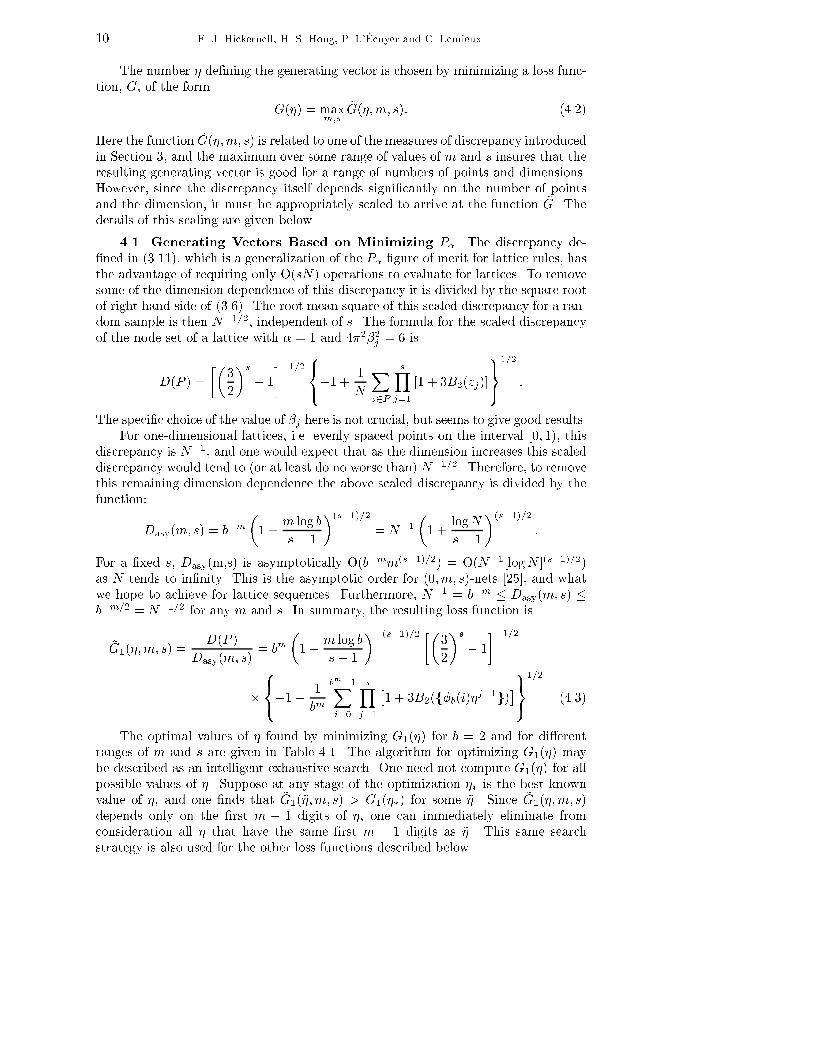
10 F. J. Hickernell, H. S. Hong, P. L'�Ecuyer and C. Lemieux.The number � de�ning the generating vector is chosen by minimizing a loss func-tion, G, of the form G(�) = maxm;s ~G(�;m; s): (4.2)Here the function ~G(�;m; s) is related to one of the measures of discrepancy introducedin Section 3, and the maximum over some range of values of m and s insures that theresulting generating vector is good for a range of numbers of points and dimensions.However, since the discrepancy itself depends signi�cantly on the number of pointsand the dimension, it must be appropriately scaled to arrive at the function ~G. Thedetails of this scaling are given below.4.1. Generating Vectors Based on Minimizing P�. The discrepancy de-�ned in (3.11), which is a generalization of the P� �gure of merit for lattice rules, hasthe advantage of requiring only O(sN) operations to evaluate for lattices. To removesome of the dimension dependence of this discrepancy it is divided by the square rootof right hand side of (3.6). The root mean square of this scaled discrepancy for a ran-dom sample is then N�1=2, independent of s. The formula for the scaled discrepancyof the node set of a lattice with � = 1 and 4�2�2j = 6 isD(P ) = ��32�s � 1��1=28<:�1 + 1N Xz2P sYj=1 [1 + 3B2(zj)]9=;1=2 :The speci�c choice of the value of �j here is not crucial, but seems to give good results.For one-dimensional lattices, i.e. evenly spaced points on the interval [0; 1), thisdiscrepancy is N�1, and one would expect that as the dimension increases this scaleddiscrepancy would tend to (or at least do no worse than) N�1=2. Therefore, to removethis remaining dimension dependence the above scaled discrepancy is divided by thefunction:Dasy(m; s) = b�m�1 + m log bs� 1 �(s�1)=2 = N�1�1 + logNs� 1�(s�1)=2 :For a �xed s, Dasy(m,s) is asymptotically O(b�mm(s�1)=2) = O(N�1[logN ](s�1)=2)as N tends to in�nity. This is the asymptotic order for (0;m; s)-nets [25], and whatwe hope to achieve for lattice sequences. Furthermore, N�1 = b�m � Dasy(m; s) �b�m=2 = N�1=2 for any m and s. In summary, the resulting loss function is~G1(�;m; s) = D(P )Dasy(m; s) = bm�1 + m log bs� 1 ��(s�1)=2 ��32�s � 1��1=2�8<:�1 + 1bm bm�1Xi=0 sYj=1 �1 + 3B2(f�b(i)�j�1g)�9=;1=2 (4.3)The optimal values of � found by minimizing G1(�) for b = 2 and for di�erentranges of m and s are given in Table 4.1. The algorithm for optimizing G1(�) maybe described as an intelligent exhaustive search. One need not compute G1(�) for allpossible values of �. Suppose at any stage of the optimization �� is the best knownvalue of �, and one �nds that ~G1(~�;m; s) > G1(��) for some ~�. Since ~G1(�;m; s)depends only on the �rst m � 1 digits of �, one can immediately eliminate fromconsideration all � that have the same �rst m � 1 digits as ~�. This same searchstrategy is also used for the other loss functions described below.

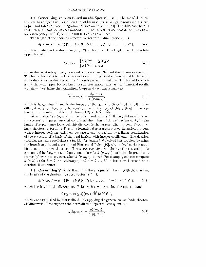
Extensible Lattice Sequences 114.2. Generating Vectors Based on the Spectral Test. The use of the spec-tral test to analyze the lattice structure of linear congruential generators is describedin [30] and tables of good integration lattices are given in [34]. The di�erence here isthat nearly all smaller lattices imbedded in the largest lattice considered must havelow discrepancy. In [34], only the full lattice was examined.The length of the shortest non-zero vector in the dual lattice L? isd2(�;m; s) = minfkkk2 : k 6= 0; k0(1; �; : : : ; �s�1) = 0 mod bmg; (4.4)which is related to the discrepancy (3.12) with r = 2. This length has the absoluteupper bound d�2(m; s) = ( sbm=s 1 � s � 8�sbm=s 8 < s (4.5)where the constants s and �s depend only on s (see [34] and the references therein).The bound for s � 8 is the least upper bound for a general s-dimensional lattice withreal-valued coordinates, and with b�m points per unit of volume. The bound for s > 8is not the least upper bound, but it is still reasonably tight, as our numerical resultswill show. We de�ne the normalized `2-spectral test discrepancy as~G2(�;m; s) = d�2(m; s)d2(�;m; s) ; (4.6)which is larger than 1 and is the inverse of the quantity St de�ned in [34]. (Thedi�erent notation here is to be consistent with the rest of this article). The lossfunction to be minimized is of the form (4.2) with ~G = ~G2.We note that 1=d2(�;m; s) can be interpreted as the (Euclidean) distance betweenthe successive hyperplanes that contain all the points of the primal lattice L, for thefamily of hyperplanes for which this distance is the largest. The problem of comput-ing a shortest vector in (4.4) can be formulated as a quadratic optimization problemwith s integer decision variables, because k can be written as a linear combinationof the s vectors of a basis of the dual lattice, with integer coe�cients. The decisionvariables are these coe�cients. (See [30] for details.) We solved this problem by usingthe branch-and-bound algorithm of Fincke and Pohst [10], with a few heuristic mod-i�cations to improve the speed. The worst-case time complexity of this algorithm isexponential in d2(�;m; s), and polynomial in s for d2(�;m; s) �xed [10]. In practice, it(typically) works nicely even when d2(�;m; s) is large. For example, one can computed2(�; 30; s) for b = 2, an arbitrary � and s = 2; : : : ; 30 in less than 1 second on aPentium-II computer.4.3. Generating Vectors Based on the `1-spectral Test. With the `1 norm,the length of the shortest non-zero vector in L? isd1(�;m; s) = minfkkk1 : k 6= 0; k0(1; �; : : : ; �s�1) = 0 mod bmg; (4.7)which is related to the discrepancy (3.12) with r = 1. One has the upper boundd1(�;m; s) � d�1(m; s) def= (s!bm)1=s;which was established by Marsaglia [37] by applying the general convex body theoremof Minkowski. This suggests the normalized `1-spectral test quantity:~G3(�;m; s) = d�1(m; s)d1(�;m; s) : (4.8)

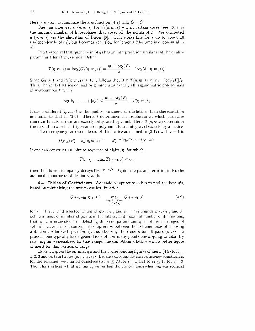
12 F. J. Hickernell, H. S. Hong, P. L'�Ecuyer and C. Lemieux.Here, we want to minimize the loss function (4.2) with ~G = ~G3.One can interpret d1(�;m; s) (or d1(�;m; s) � 1 in certain cases; see [30]) asthe minimal number of hyperplanes that cover all the points of P . We computedd1(�;m; s) via the algorithm of Dieter [6], which works �ne for s up to about 10(independently of m), but becomes very slow for larger s (the time is exponential ins). The `1-spectral test quantity in (4.8) has an interpretation similar that the qualityparameter t for (t;m; s)-nets. De�neT (�;m; s) = logb( ~G3(�;m; s)) = m+ logb(s!)s � logb(d1(�;m; s)):Since ~G3 � 1 and d1(�;m; s) � 1, it follows that 0 � T (�;m; s) � [m + logb(s!)]=s.Thus, the rank-1 lattice de�ned by � integrates exactly all trigonometric polynomialsof wavenumber k whenlog(jk1j+ � � �+ jksj) � m+ logb(s!)s � T (�;m; s):If one considers T (�;m; s) as the quality parameter of the lattice, then this conditionis similar to that in (2.5). There, t determines the resolution at which piecewiseconstant functions that are exactly integrated by a net. Here, T (�;m; s) determinesthe resolution at which trigonometric polynomials are integrated exactly by a lattice.The discrepancy for the node set of this lattice as de�ned in (3.12) with r = 1 isDF;1(P ) = d1(�;m; s)�� = (s!)��=sb�T (�;m;s)N��=s:If one can construct an in�nite sequence of digits, �, for whichT (�; s) = maxm T (�;m; s) <1;then the above discrepancy decays like N��=s. Again, the parameter � indicates theassumed smoothness of the integrands.4.4. Tables of Coe�cients. We made computer searches to �nd the best �'s,based on minimizing the worst-case loss functionGi(�;m0;m1; s1) = maxm0�m�m11�s�s1 ~Gi(�;m; s) (4.9)for i = 1; 2; 3, and selected values of m0, m1, and s1. The bounds m0, m1, and s1de�ne a range of number of points in the lattice, and maximal number of dimensions,that we are interested in. Selecting di�erent parameters � for di�erent ranges ofvalues of m and s is a convenient compromise between the extreme cases of choosinga di�erent � for each pair (m; s), and choosing the same � for all pairs (m; s). Inpractice one typically has a general idea of how many points one is going to take. Byselecting an � specialized for that range, one can obtain a lattice with a better �gureof merit for this particular range.Table 4.1 gives the optimal �'s and the corresponding �gures of merit (4.9) for i =1; 2; 3 and certain triples (m0;m1; s1). Because of computational e�ciency constraints,for the searches, we limited ourselves to m1 � 20 for i = 1 and to s1 � 10 for i = 3.Then, for the best � that we found, we veri�ed the performance when m0 was reduced

Extensible Lattice Sequences 13or when m1 or s1 was increased, and retained the smallest m0 and largest m1 and s1for which Gi was unchanged. The table also gives the value of Gi;min(�;m0;m1; s1),de�ned by replacing max by min in (4.9). This best-case �gure tells us the range ofvalues taken by ~Gi(�;m; s) over the given region. We also made exhaustive searcheswith s1 = 15 for all the entries where i = 1 or 2 in the table, and obtained the samevalues of � and Gi(�;m0;m1; s1) in all cases.Table 4.1Values of � de�ning generating vectors of the form (4.1) for rank-1 lattice sequences with baseb = 2, and minimizing (4.9).i m0 m1 s1 � Gi(�;m0;m1; s1) Gi;min(�;m0;m1; s1)1 0 17 32 17797 4.11 0.781 0 12 32 203 2.33 0.781 0 16 32 17797 3.57 0.781 13 20 32 407641 5.86 0.972 0 17 25 1267 2.05 1.002 1 16 34 12915 1.90 1.002 6 12 33 1571 1.88 1.102 8 17 32 11335 1.83 1.032 14 20 37 156487 1.76 1.052 15 24 32 4450341 1.79 1.073 6 16 12 237 2.25 1.073 6 12 10 53 2.25 1.143 10 16 11 173 2.25 1.153 14 21 11 391485 2.00 1.013 16 24 10 1459305 2.10 1.115. Estimating Quadrature Error. The advantage of an extensible lattice se-quence is that N need not be speci�ed in advance. Therefore, in practice one wouldestimate the quadrature error for an initial lattice, and continue to increase the latticesize until the quadrature error meets the desired tolerance. Although the discrepancy,D(P ), is a good measure for the quality of a set P , it cannot be used directly for errorestimation. The worst case error bounds (3.1) are often quite conservative, and thereis no easy way to estimate the variation of the integrand. The average case errorgiven, (3.4), is sensitive to how one de�nes the kernel | multiplying the kernel by afactor of c2 changes the average case error by a factor of c.Quadrature error estimates for lattice rules have been investigated by [5, 28,53]. Two di�erent kinds of quadrature rules and error estimates have been proposed.Both involve estimating the error for Q(f ;P ) in terms of Q(f ;P ) and Q(f ;Pl), l =1; : : : ;M , where the Pl are node sets of lattices and P = P1 [ � � � [ PM .The method proposed in [53] takes P to be composed of 2s shifted copies of arank-1 lattice. Rather than considering copy rules, we take Pl to be the node sets ofshifted lattices of size bm1 imbedded in the extensible lattice described in Section 2.4:Pl = ff�b((l � 1)bm1 + i)h+�g : i = 0; : : : ; bm1 � 1g ; l = 1; : : : ;M; (5.1a)P = ff�b(i)h+�g : i = 0; : : : ;Mbm1 � 1g ; (5.1b)

14 F. J. Hickernell, H. S. Hong, P. L'�Ecuyer and C. Lemieux.Another quadrature rule and error estimate takes the Pl to be independent ran-dom shifts of a lattice. This can be done by taking:Pl = ff�b(i)h+�lg : i = 0; : : : ; bm1 � 1g ; l = 1; : : : ;M; (5.2a)P = ff�b(i)h+�lg : i = 0; : : : ; bm1 � 1; l = 1; : : : ;Mg ; (5.2b)where the �l are independent, uniformly distributed random vectors in [0; 1]s.Note that for both (5.1) and (5.2) the set P can be extended in size as necessaryby increasing m1. The theory behind the error estimates for cases (5.1) and (5.2) aregiven in the following theorem.Theorem 5.1. Suppose that a quadrature rule Q(�;P ) based on some arbitraryP , as given in (1.1), is the average value of the quadrature rules based on the setsP1; : : : ; PM , that is, Q(�;P ) = 1M MXl=1 Q(�;Pl): (5.3)First, consider the case where the integrands are random functions from a samplespace A as described in the paragraph preceding (3.4). Then it follows thatEf2A[I(f)�Q(f ;P )]2= (�1 + 1M MXl=1 �D(Pl)D(P ) �2)�1 1M MXl=1 Ef2A[Q(f ;Pl)�Q(f ;P )]2; (5.4)where D is the discrepancy based on the covariance kernel for A.Secondly, consider the case of a �xed integrand, f , but where the Pl are randomshifts of a set P0, that is,P = P1 [ � � � [ PM ; Pl = ffz +�lg : z 2 P0g; (5.5)for independent, uniformly distributed �1; : : : ;�M . ThenE�lf[I(f)�Q(f ;P )]2g = 1M(M � 1) MXl=1 E�l [Q(f ;Pl)�Q(f ;P )]2: (5.6)Proof. Assuming that the quadrature rules satisfy (5.3), it follows that the meansquare deviation of the Q(f ;Pl) from Q(f ;P ) may be written as1M MXl=1 [Q(f ;Pl)�Q(f ;P )]2 = 1M MXl=1f[I(f)�Q(f ;P )]� [I(f)�Q(f ;Pl)]g2= �[I(f)�Q(f ;P )]2 + 1M MXl=1 [I(f)�Q(f ;Pl)]2: (5.7)If the integrand is a random function from a sample space A with covariance kernelK, then average case error analysis in (3.4) plus (5.7) leads to the following equations:Ef2A[I(f)�Q(f ;P )]2 = [D(P )]2;Ef2A[I(f)�Q(f ;Pl)]2 = [D(Pl)]2;Ef2A( 1M MXl=1 [Q(f ;Pl)�Q(f ;P )]2) = �[D(P )]2 + 1M MXl=1 [D(Pl)]2:

Extensible Lattice Sequences 15The equations above may be rearranged to give (5.4).The quadrature error for rule Q(f ;P ) may also be written as:[I(f)�Q(f ;P )]2 = ( 1M MXl=1 [I(f)�Q(f ;Pl)])2= 1M2 MXl=1 [I(f)�Q(f ;Pl)]2+ 2M2 X1�k<l�M [I(f)�Q(f ;Pi)][I(f)�Q(f ;Pl)]:Substituting the sum of the [I(f)�Q(f ;Pl)]2 by equation (5.7) gives:[I(f)�Q(f ;P )]2 = 1M(M � 1) MXl=1 [Q(f ;Pl)�Q(f ;P )]2+ 2M(M � 1) X1�k<l�M [I(f)�Q(f ;Pk)][I(f)�Q(f ;Pl)]: (5.8)If the Pl are random shifts as in (5.5), then the expected value of the term [I(f) �Q(f ;Pk)][I(f)�Q(f ;Pl)] vanishes for all k 6= l and taking the expected value of (5.8)yields (5.6).Some remarks are in order to explain the assumptions and conclusions of theabove theorem. These are given below.Assumption (5.3), and thus conclusion (5.4), holds for both the cases (5.1) and(5.2) above. In fact, this part of the theorem holds for any imbedded rule or any rulewhere the Pl all contain the same number of points, and their union is P or multiplecopies of P . For example, (5.4) would apply to the case where P is a (t;m; s)-netmade up of a union of subnets Pl.Assumption (5.5), and therefore conclusion (5.6) holds for (5.2). There is a di�-culty if one tries to derive a result like (5.6) for an imbedded rule of the form (5.1),where � is a random shift. The argument leading to (5.6) assumes that the points indi�erent Pl are uncorrelated, which is not true for (5.1). However, if the extensiblelattice is a good one, it is expected that the terms [I(f)�Q(f ;Pk)][I(f)�Q(f ;Pl)]in (5.8) are on average negative. Under this assumption one may then conclude thatthe right hand side of (5.6) is a conservative (too large) upper bound on the expectedsquare quadrature error.The factor in (5.4) above involving the discrepancies of P and the Pl does notdepend strongly on the particular choice of discrepancy, but only on the asymptoticrate of decay. If, for example, D(P ) � CN�� for some unknown C, but known �,where N is the number of points in P , thenEf2A[I(f)�Q(f ;P )]2 � 1M(M2� � 1) MXl=1 Ef2A[Q(f ;Pl)�Q(f ;P )]2: (5.9)Although conclusions (5.6) and (5.9) are derived under di�erent assumptions,they both suggest error estimates of the form[I(f)�Q(f ;P )]2 / c2M(M2� � 1) MXl=1 [Q(f ;Pl)�Q(f ;P )]2; (5.10)

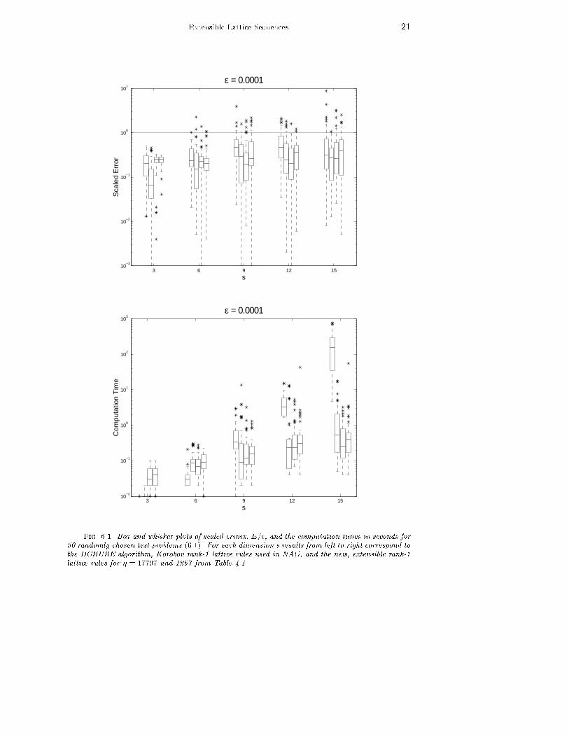
16 F. J. Hickernell, H. S. Hong, P. L'�Ecuyer and C. Lemieux.where � = 1=2 for (5.6) and � indicates the rate of decay of the discrepancy for (5.9).The factor c > 1 depends on how conservative one wishes to be. The Chebyshevinequality implies that the above inequality will hold \at least" 100(1� c�2)% of thetime. Error estimate (5.10) leads to the stopping criteria:c2M(M � 1) MXl=1 [Q(f ;Pl)�Q(f ;P )]2 < �2; (5.11)where � is the absolute error tolerance. Note that if the stopping criteria is not met,one would normally increase the size of the Pl by increasingm1, rather than increasingthe number of the Pl by increasing M .For some high dimensional problems the discrepancy of a lattice (or other lowdiscrepancy set) may decay as slowly as the Monte Carlo rate of O(N�1=2) for smallN (see [18, 41]). Therefore, even when using (5.9), it may be advisable to make aconservative choice of � = 1=2. This choice makes the approach of error estimate(5.9), based on random integrands, equivalent to that of (5.6), based on randomlyshifted Pl.Sloan and Joe [53, Section 10.3] suggest an error estimate of the form[I(f)�Q(f ;P )]2 / c2s sXl=1 [Q(f ;Pl)�Q(f ;P )]2;where P is formed from 2s copies of a rank-1 lattice, and each Q(f ;Pl) is an imbeddedrule based on half of the points in P . Although this case does not exactly �t Theorem5.1, the arguments in the proof can be modi�ed to obtain a result similar to to (5.4):Ef2A[I(f)�Q(f ;P )]2= (�1 + 1s sXl=1 �D(Pl)D(P ) �2)�1 1s sXl=1 Ef2A[Q(f ;Pl)�Q(f ;P )]2:This would suggest that the error estimation formula of Sloan and Joe is reasonablewhen D(Pl) � p2D(P ) on average. The disadvantage of 2s-copy rules is that theyrequire at least 2s points, which may be unmanageable for large s.To summarize, both imbedded lattice rules, (5.1), and independent random shiftsof lattices, (5.2), have similar error estimates, (5.10), and stopping criteria, (5.11).The advantage of the independent random shifts approach is that, the theory holdsfor any integrand, not the average over a space of integrands. One advantage of theimbedded rules approach is that one need only generate a single extensible lattice.Furthermore, the set P for the imbedded rule is the node set of a lattice (if M is apower of b), which is never the case for the independent random shifts approach. Thus,the accuracy of the imbedded rule approach is likely to be better. In the examples inthe next section, the imbedded lattice rules based on (5.1) are used.6. Examples of Multidimensional Quadrature. Two example problems arechosen to demonstrate the performance of the new rank-1 lattice sequences proposed inSection 2.4. The �rst example is the computation of multivariate normal probabilitiesand the second is the evaluation of a multidimensional integral arising in physicsproblems.

Extensible Lattice Sequences 176.1. Multivariate Normal Probabilities. Consider the following multivariatenormal probability: 1pj�j(2�)s Z b1a1 � � �Z bsas e� 12 �0��1� d�: (6.1a)where, a and b are known s-dimensional vectors, and � is a given s�s positive de�nitecovariance matrix. Some aj and/or bj may be in�nite.Unfortunately, the original form is not well-suited for numerical quadrature.Therefore, Alan Genz [12] proposed a transformation of variables that results inan integral over an s � 1-dimensional unit cube. See [12, 13] for the details of thetransformation, and see [13, 15] for comparisons of di�erent methods for calculatingmultivariate normal probabilities.The particular test problem is one considered by [13, 24] and may be describedas follows: a1 = � � � = as = �1; (6.1b)bj i.i.d. uniformly on [0;ps]; (6.1c)� generated randomly according to [13, 38]: (6.1d)Numerical comparisons were made using three types of algorithms:i. the adaptive algorithm DCHURE [2],ii. an older Korobov rank-1 lattice rule with a di�erent generating vector foreach N and s | this algorithm is a part of NAG and is used in [5, 12], andiii. the new rank-1 lattice sequences proposed in Section 2.4 with generatingvectors given in Table 4.1For the second and third algorithms we applied the periodizing transformation x0j =j2xj � 1j to the integrand over the unit cube. This appears to increase the accuracyof the lattice rule methods. The computations were carried out in FORTRAN on aUnix work station in double precision. The absolute error tolerance was chosen to be� = 10�4, and this was compared with the actual error E. Since the true value of theintegral is unknown for this test problem, the value given by the Korobov algorithmwith a tolerance of � = 10�8 was used as the \exact" value for computing the error.For the new rank-1 lattice sequences the stopping criterion (5.11) was used with Mbetween 4 and 7 and c = 3.For each dimension 50 random test problems were generated and solved by thevarious quadrature methods. The scaled absolute errors E=� and the computationtimes in seconds are given in the box and whisker plots of Fig. 6.1. The boxes containthe middle half of the values and the whiskers give the range of most values exceptthe outliers (denoted by �).Ideally, the scaled error should nearly always be less than one, otherwise theerror estimate is not conservative enough. On the other hand if the scaled error is toosmall, then the error estimate is too conservative. Fig. 6.1 shows that the adaptiverule performs well for smaller dimensions, but underestimates the error and is quiteslow in higher dimensions. The lattice rules do well even in higher dimensions, andthe new rank-1 lattice sequences appear to be faster than the older Korobov-typerule. This is likely due to the fact that the lattice sequences proposed here can re-usethe old points when N must be increased.

18 F. J. Hickernell, H. S. Hong, P. L'�Ecuyer and C. Lemieux.6.2. A Multidimensional Integral from Physics. Keister [29] consideredthe following multidimensional integral that has applications in physics:ZRs cos(kxk2)e�kxk22 dx = �s=2 Z[0;1)s cos0@vuut sXj=1 [��1(yj)]22 1A dy; (6.2)where � denotes the standard Gaussian distribution function. Keister gave an ex-act formula for the answer and compared the quadrature methods of McNamee andStenger [39] and Genz and Patterson [11, 51] for evaluating this integral. Later, Pa-pageorgiou and Traub [49] applied the generalized Faure sequence from FINDER tothis problem.The results of numerical experiments for the above integral for dimension 25 areshown in Figure 6.2. The exact value of the integral is reported in [49]. To beconsistent with the numerical results reported in [29, 49], we did not perform errorestimation, but just computed the actual error for each kind of numerical method asa function of N , the number of points. Because ��1(0) = �1 there is a technicaldi�culty with using an unshifted lattice rule, so when performing the numerical ex-periments the lattice sequences were given random shifts (modulo 1). Box and whiskerplots show how well the new rank-1 lattice sequences perform for 50 random shifts.According to Figure 6.2 the generalized Faure sequence (in base 29) and thelattice sequence perform much better than the other two rules. In some cases thelattice sequences perform better than the generalized Faure sequence.7. Conclusion. Lattice rules are simpler to code than digital nets. Given theconstruction in Section 2.4, it is now possible to have extensible lattice sequences inthe same way that one has (t; s)-sequences. Good generating vectors for these latticesequences may be found by using the spectral test or minimizing other discrepancymeasures, as shown in Section 4. The performance of these lattice rules is in manycases comparable to other multidimensional quadrature rules and in some cases su-perior.Acknowledgments. Thanks to Alan Genz for making available his software forcomputing multivariate normal distributions. Also thanks to Joe Traub and Anargy-ros Papageorgiou for making available the FINDER software.REFERENCES[1] M. Abramowitz and I. A. Stegun, eds., Handbook of Mathematical Functions with Formulas,Graphs and Mathematical Tables, U. S. Government Printing O�ce, Washington, DC,1964.[2] J. Bernsten, T. O. Espelid, and A. Genz, An adaptive algorithm for the approximate cal-culation of multiple integrals, ACM Trans. Math. Software, 17 (1991), pp. 437{451.[3] R. E. Caflisch, Monte Carlo and quasi-Monte Carlo methods, Acta Numer., 7 (1998), pp. 1{49.[4] R. E. Caflisch, W. Morokoff, and A. Owen, Valuation of mortgage backed securities usingBrownian bridges to reduce e�ective dimension, J. Comput. Finance, 1 (1997), pp. 27{46.[5] R. Cranley and T. N. L. Patterson, Randomization of number theoretic methods for multipleintegration, SIAM J. Numer. Anal., 13 (1976), pp. 904{914.[6] U. Dieter, How to calculate shortest vectors in a lattice, Math. Comp., 29 (1975), pp. 827{833.[7] K. Entacher, P. Hellekalek, and P. L'�Ecuyer, Quasi-Monte Carlo node sets from linearcongruential generators, in Niederreiter and Spanier [46].[8] K. T. Fang and Y. Wang, Number-Theoretic Methods in Statistics, Chapman and Hall, NewYork, 1994.

Extensible Lattice Sequences 19[9] H. Faure, Discr�epance de suites associ�ees �a un syst�eme de num�eration (en dimension s), ActaArith., 41 (1982), pp. 337{351.[10] U. Fincke and M. Pohst, Improved methods for calculating vectors of short length in a lattice,including a complexity analysis, Math. Comp., 44 (1985), pp. 463{471.[11] A. Genz, A Lagrange extrpolation algorithm for sequences of approximations to multiple inte-grals, SIAM J. Sci. Stat. Comput., 3 (1982), pp. 160{172.[12] , Numerical computation of multivariate normal probabilities, J. Comput. Graph.Statist., 1 (1992), pp. 141{150.[13] , Comparison of methods for the computation of multivariate normal probabilities, Com-puting Science and Statistics, 25 (1993), pp. 400{405.[14] S. Haber, Parameters for integrating periodic functions of several variables, Math. Comp., 41(1983), pp. 115{129.[15] V. Hajivassiliou, D. McFadden, and P. Ruud, Simulation of multivariate normal rectangleprobabilities and their derivatives theoretical and computational results, J. Econometrics,72 (1996), pp. 85{134.[16] P. Hellekalek, On the assessment of random and quasi-random point sets, in Hellekalek andLarcher [17], pp. 49{108.[17] P. Hellekalek and G. Larcher, eds., Random and Quasi-Random Point Sets, vol. 138 ofLecture Notes in Statistics, Springer-Verlag, New York, 1998.[18] F. J. Hickernell, A comparison of random and quasirandom points for multidimensionalquadrature, in Niederreiter and Shiue [45], pp. 213{227.[19] , The mean square discrepancy of randomized nets, ACM Trans. Model. Comput. Simul.,6 (1996), pp. 274{296.[20] , Quadrature error bounds with applications to lattice rules, SIAM J. Numer. Anal., 33(1996), pp. 1995{2016. corrected printing of Sections 3-6 in ibid., 34 (1997), 853{866.[21] , A generalized discrepancy and quadrature error bound, Math. Comp., 67 (1998),pp. 299{322.[22] , Lattice rules: How well do they measure up?, in Hellekalek and Larcher [17], pp. 109{166.[23] , What a�ects the accuracy of quasi-Monte Carlo quadrature?, in Niederreiter andSpanier [46]. to appear.[24] F. J. Hickernell and H. S. Hong, Computing multivariate normal probabilities using rank-1lattice sequences, in Proceedings of the Workshop on Scienti�c Computing, G. H. Golub,S. H. Lui, F. T. Luk, and R. J. Plemmons, eds., Hong Kong, 1997, Springer-Verlag, Singa-pore, pp. 209{215.[25] , The asymptotic e�ciency of randomized nets for quadrature, Math. Comp., 68 (1999),pp. 767{791.[26] E. Hlawka, Funktionen von beschr�ankter Variation in der Theorie der Gleichverteilung, Ann.Mat. Pura Appl., 54 (1961), pp. 325{333.[27] L. K. Hua and Y. Wang, Applications of Number Theory to Numerical Analysis, Springer-Verlag and Science Press, Berlin and Beijing, 1981.[28] S. Joe, Randomization of lattice rules for numerical multiple integration, J. Comput. Appl.Math., 31 (1990), pp. 299{304.[29] B. D. Keister, Multidimensional quadrature algorithms, Computers in Physics, 10 (1996),pp. 119{122.[30] D. E. Knuth, The Art of Computer Programming, Volume 2: Seminumerical Algorithms,Addison-Wesley, Reading, Mass., third ed., 1997.[31] N. M. Korobov, The approximate computation of multiple integrals, Dokl. Adad. Nauk. SSR,124 (1959), pp. 1207{1210. (Russian).[32] G. Larcher, On the distribution of digital sequences, in Monte Carlo and quasi-Monte Carlomethods 1996, H. Niederreiter, P. Hellekalek, G. Larcher, and P. Zinterhof, eds., vol. 127of Lecture Notes in Statistics, Springer-Verlag, New York, 1997, pp. 109{123.[33] P. L'�Ecuyer, Random number generation, in Handbook of Simulation, J. Banks, ed., Wiley,1998, ch. 4, pp. 93{137.[34] P. L'�Ecuyer, Tables of linear congruential generators of di�erent sizes and good lattice struc-ture, Math. Comp., 68 (1999), pp. 249{260.[35] C. Lemieux and P. L'�Ecuyer, E�ciency improvement by lattice rules for pricing asian op-tions, in Proc. 1998 Winter Simulation Conference, IEEE Press, 1998, pp. 579{586.[36] , A comparison of Monte Carlo, lattice rules and other low-discrepancy point sets, inNiederreiter and Spanier [46].[37] G. Marsaglia, Random numbers fall mainly in the planes, Proc. Natl. Acad. Sci. USA, 60(1968), pp. 25{28.

20 F. J. Hickernell, H. S. Hong, P. L'�Ecuyer and C. Lemieux.[38] G. Marsaglia and I. Olkin, Generating correlation matrices, SIAM J. Sci. & Statist. Com-put., 5 (1984), pp. 470{475.[39] J. McNamee and F. Stenger, Construction of fully symmetric numerical integration formu-las, Numer. Math., 10 (1967), pp. 327{344.[40] W. J. Morokoff, Generating quas-random paths for stochastic processes, SIAM Rev., 40(1998), pp. 765{788.[41] W. J. Morokoff and R. E. Caflisch, Quasi-random sequences and their discrepancies, SIAMJ. Sci. Comput., 15 (1994), pp. 1251{1279.[42] , Quasi-Monte Carlo integration, J. Comput. Phys., 122 (1995), pp. 218{230.[43] H. Niederreiter, Points and sequences with small discrepancy, Monatsh. Math., 104 (1987),pp. 273{337.[44] , Random Number Generation and Quasi-Monte Carlo Methods, SIAM, Philadelphia,1992.[45] H. Niederreiter and P. J.-S. Shiue, eds., Monte Carlo and Quasi-Monte Carlo Methods inScienti�c Computing, vol. 106 of Lecture Notes in Statistics, Springer-Verlag, New York,1995.[46] H. Niederreiter and J. Spanier, eds., Monte Carlo and Quasi-Monte Carlo Methods 1998,Springer-Verlag, Berlin, 1999.[47] H. Niederreiter and C. Xing, Quasirandom points and global function �elds, in Finite Fieldsand Applications, London Math. Society Lecture Note Series, Cambridge University Press,1996, pp. 269{296.[48] A. Papageorgiou and J. F. Traub, Beating Monte Carlo, Risk, 9 (1996), pp. 63{65.[49] , Faster evaluation of multidimensional integrals, Computers in Physics, 11 (1997),pp. 574{578.[50] S. Paskov and J. Traub, Faster valuation of �nancial derivatives, J. Portfolio Management,22 (1995), pp. 113{120.[51] T. N. L. Patterson, The optimum addition of points to quadrature formulae, Math. Comp.,22 (1968), pp. 847{856.[52] I. H. Sloan, Lattice methods for multiple integration, J. Comput. Appl. Math., 12 & 13 (1985),pp. 131{143.[53] I. H. Sloan and S. Joe, Lattice Methods for Multiple Integration, Oxford University Press,Oxford, 1994.[54] I. H. Sloan and P. J. Kachoyan, Lattice methods for multiple integration: Theory, erroranalysis and examples, SIAM J. Numer. Anal., 24 (1987), pp. 116{128.[55] I. H. Sloan and H. Wo�zniakowski, An intractability result for multiple integration, Math.Comp., 66 (1997), pp. 1119{1124.[56] I. M. Sobol', The distribution of points in a cube and the approximate evaluation of integrals,U.S.S.R. Comput. Math. and Math. Phys., 7 (1967), pp. 86{112.[57] , Multidimensional Quadrature Formulas and Haar Functions (in Russian), Izdat.\Nauka", Moscow, 1969.[58] J. Spanier, Quasi-Monte Carlo methods for particle transport problems, in Niederreiter andShiue [45], pp. 121{148.[59] J. Spanier and E. H. Maize, Quasi-random methods for estimating integrals using relativelysmall samples, SIAM Rev., 36 (1994), pp. 18{44.[60] T. T. Warnock, Computational investigations of low discrepancy point sets, in Applicationsof Number Theory to Numerical Analysis, S. K. Zaremba, ed., Academic Press, New York,1972, pp. 319{343.[61] H. Wo�zniakowski, Average case complexity of multivariate integration, Bull. Amer. Math.Soc., 24 (1991), pp. 185{194.[62] S. K. Zaremba, Some applications of multidimensional integration by parts, Ann. Polon.Math., 21 (1968), pp. 85{96.

Extensible Lattice Sequences 21

3 6 9 12 1510

−3

10−2

10−1

100

101

Sca

led

Err

or

ε = 0.0001

s

3 6 9 12 1510

−2

10−1

100

101

102

103

Com

puta

tion

Tim

e

ε = 0.0001

sFig. 6.1. Box and whisker plots of scaled errors, E=�, and the computation times in seconds for50 randomly chosen test problems (6.1). For each dimension s results from left to right correspond tothe DCHURE algorithm, Korobov rank-1 lattice rules used in NAG, and the new, extensible rank-1lattice rules for � = 17797 and 1267 from Table 4.1.

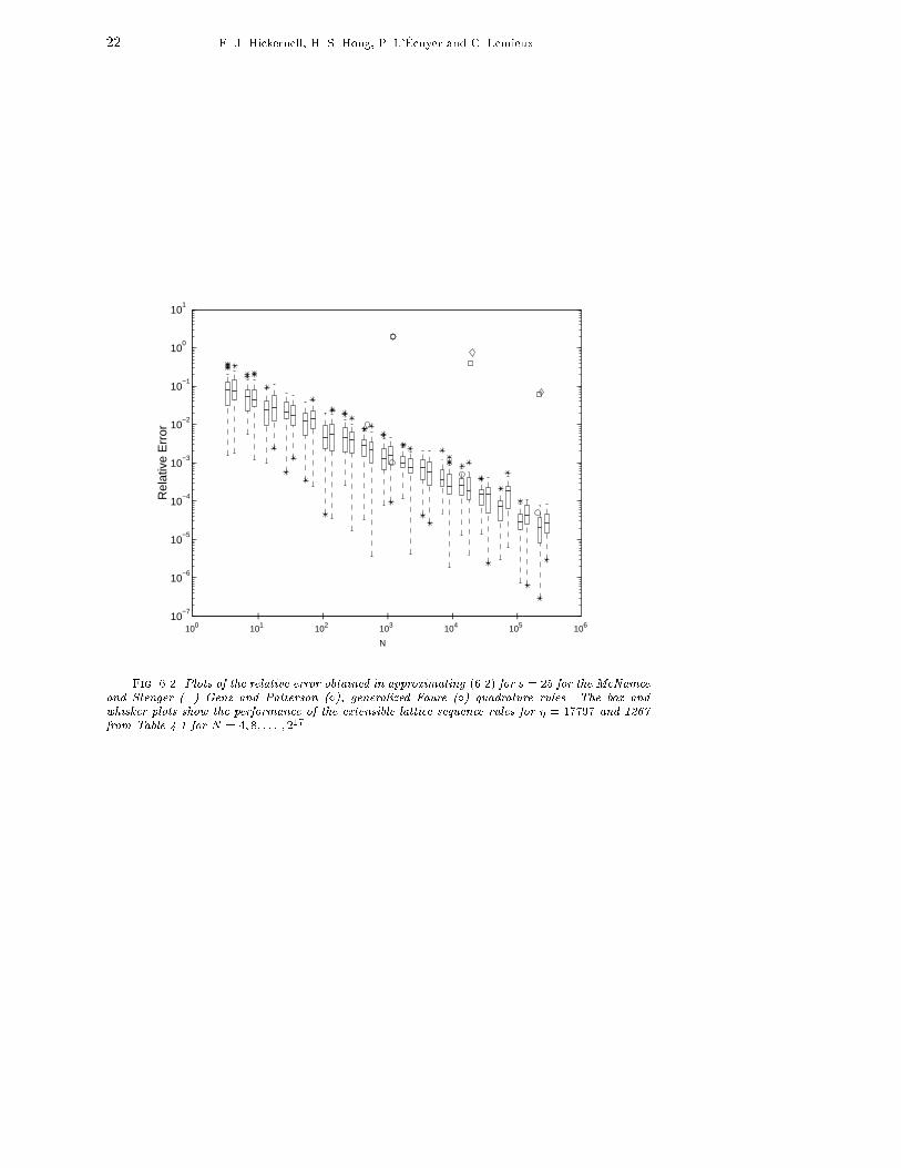
22 F. J. Hickernell, H. S. Hong, P. L'�Ecuyer and C. Lemieux.

10−7

10−6

10−5

10−4

10−3

10−2

10−1

100

101

Rel

ativ

e E

rror

l l l l l100 101 102 103 104 105 106

NFig. 6.2. Plots of the relative error obtained in approximating (6.2) for s = 25 for the McNameeand Stenger (�) Genz and Patterson (�), generalized Faure (�) quadrature rules. The box andwhisker plots show the performance of the extensible lattice sequence rules for � = 17797 and 1267from Table 4.1 for N = 4; 8; : : : ; 217.