Extending the Observer Model for Human Orientation ...

by

NAVAL MEDICAL RESEARCH UNIT DAYTON

v.3 Oct2019

v.3 Oct2019

1

Extending the Observer Model for Human Orientation Perception

to Include In-Flight Perceptual Thresholds

Torin K. Clark1, Jamie Voros1, Daniel M. Merfeld2,3, and Henry P. Williams3

1University of Colorado – Boulder 2Ohio State University 3Naval Medical Research Unit Dayton

2

Abstract

Pilots of high performance fixed- and rotary-wing aircraft have to make decisions about

their vehicle’s motion; for example, deciding if the helicopter is drifting forward or

backwards. Translation direction-recognition thresholds have been empirically

quantified in the laboratory, but less so in flight, where complex six degree-of-freedom

motions occur over more sustained durations and include vibrations. To investigate self-

motion vestibular perceptual thresholds, we have added a decision-making dynamic

element to an existing, state-of-the-art computational model for human spatial

orientation perception. Experiments across a range of decision-making paradigms

suggest humans tend to process perceptual information in a manner similar to a high-

pass filter, in which only the most recent information contributes to the decision. We

then simulated the model to predict human perceptual thresholds for translation, which

were compared to human subject experiments in laboratory or flight. While the model

was able to capture laboratory empirical thresholds across a range of motion durations,

those observed in a recent helicopter flight experiment were much higher than

predicted. Using the model, we ruled out potential causes of this discrepancy, including

the respective motion duration, the motion’s acceleration and deceleration being

symmetric versus having a longer deceleration, and the full six degree-of-freedom

components of the helicopter motions. We conclude with a discussion of potential

alternative explanations of the apparently much higher thresholds observed in the flight

experiment and propose future experiments to evaluate these hypotheses.

Understanding vestibular thresholds is important as pilots who misperceive these

motions will experience some form of spatial disorientation, which continues to be a

leading cause of fatal mishaps.

Introduction and Motivation

In everyday life, humans often have to make decisions about how they are moving, for example, “Am I

falling forwards or am I falling backwards?” Pilots of high performance aircraft and helicopters have to

make similar decisions, but with the added challenge of complex six degree-of-freedom motions that are

often large and sustained. Alternatively, motions may be relatively small and not be well perceived by

the pilot. For example, a helicopter may drift (i.e., translate in the horizontal plane) at a small enough

magnitude such that the pilot may not realize they are drifting until the motion becomes larger. This is

an example of spatial disorientation, where a pilot misperceives the attitude, position, or motion of

his/her aircraft relative to the Earth’s surface, gravitational vertical, or other reference points (Benson

1978). Across military, commercial, and general aviation, spatial disorientation continues to be a leading

cause of fatal mishaps (Williams, Horning et al. 2018, Boeing 2019, Newman and Rupert 2020).

To properly capture these motion misperception scenarios, we have added “threshold” (i.e., decision-

making – “Am I drifting, and is it to the left or right?”) dynamic elements to an existing, state-of-the-art

computational model for human spatial orientation perception. Model predictions are compared to data

from human subject experiments in laboratory or flight, where available. We conclude with a discussion

3

of potential alternative explanations for human thresholds of drift perception and propose future

experiments to distinguish between these alternatives and further validate these model extensions.

Background

In order to capture the sensory and central processing required for spatial orientation perception,

computational models have been proposed (Merfeld, Young et al. 1993, MacNeilage, Ganesan et al.

2008). These types of models have been successful in mimicking a range of illusory perceptions

observed in laboratory paradigms, and more recently have been applied to determine the potential of

pilot spatial disorientation during fixed-wing and rotary-wing flight. A leading computational model,

known as the “observer model”, is based upon the hypotheses that the brain uses internal models of

sensory dynamics and kinematic relationships to compare expected sensory responses to those actually

measured. In the model, the differences between sensory measurements and those expected are

weighted and drive central estimates (i.e., perceptions) of motion states, such as angular velocity, linear

acceleration, and gravity. For a review of the observer model, see Clark, Newman et al., 2019. While the

model is capable of simulating complex full six degree-of-freedom passive motions, critically, it predicts

human orientation perception (i.e., continuous estimates of motion states, like linear acceleration over

time), as opposed to discrete decisions about self-motion perception.

There is growing evidence that when the brain needs to make a decision about motion perception (such

as during a threshold task — “Did I move left or did I move right?”), additional neural processing is

performed (Merfeld, Clark et al. 2016). Specifically, the decision-making appears to be well modeled as a

high-pass filter, in which lower frequency sensory/perception information (i.e., that from a while ago) is

filtered out, and only higher frequency (i.e., more recent) information is used to help make the decision

(Figure 1).

Figure 1: Evidence suggests that a decision-making high-pass filter is applied to the central orientation perception in order to

produce a decision variable. In this example, angular velocity (ω) is transduced by the semicircular canals (SCC), producing an

afferent neural response (�̃�). The sensory dynamics of the semicircular canals are often modeled as a high-pass filter with a time

constant (τSCC) of about 5.7 seconds. The brain then processes this to yield a central perception of angular velocity (�̂�). This

neural mechanism, referred to as “velocity storage”, extends the time constant of the high-pass filtering for rotation perception

(from ω to �̂�, τper) to approximately 23 seconds. The observer model captures these processes and resulting dynamics. It is

hypothesized that the brain then further high-pass filters this central perception (�̂�) to produce a decision variable (d). The

cutoff frequency (fCO) of this high-pass filter is approximately 0.25 Hz (i.e., 4 seconds per cycle) which corresponds to a time

constant for decision-making (τDM) of approximately 0.6 seconds (τ=1/(2πf)). Figure after (Merfeld, Clark et al. 2016).

While Figure 1 shows the decision-making high-pass filter along the pathways for angular velocity (ω), it

has also been observed to explain decisions regarding perception of translation (i.e., “Did I move left or

4

did I move right?”), as well as scenarios beyond self-motion (e.g., “Is an illuminated bar tilted to the left

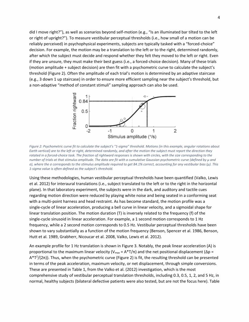
or right of upright?”). To measure vestibular perceptual thresholds (i.e., how small of a motion can be

reliably perceived) in psychophysical experiments, subjects are typically tasked with a “forced-choice”

decision. For example, the motion may be a translation to the left or to the right, determined randomly,

after which the subject must decide and respond whether they felt they moved to the left or right. Even

if they are unsure, they must make their best guess (i.e., a forced-choice decision). Many of these trials

(motion amplitude + subject decision) are then fit with a psychometric curve to calculate the subject’s

threshold (Figure 2). Often the amplitude of each trial’s motion is determined by an adaptive staircase

(e.g., 3 down 1 up staircase) in order to ensure more efficient sampling near the subject’s threshold, but

a non-adaptive “method of constant stimuli” sampling approach can also be used.

Figure 2: Psychometric curve fit to calculate the subject’s "1-sigma" threshold. Motions (in this example, angular rotations about Earth vertical) are to the left or right, determined randomly, and after the motion the subject must report the direction they rotated in a forced-choice task. The fraction of rightward responses is shown with circles, with the size corresponding to the number of trials at that stimulus amplitude. The data are fit with a cumulative Gaussian psychometric curve (defined by µ and σ), where the σ corresponds to the stimulus amplitude required to get 84.1% correct, accounting for any vestibular bias (µ). This 1-sigma value is often defined as the subject’s threshold.

Using these methodologies, human vestibular perceptual thresholds have been quantified (Valko, Lewis

et al. 2012) for interaural translations (i.e., subject translated to the left or to the right in the horizontal

plane). In that laboratory experiment, the subjects were in the dark, and auditory and tactile cues

regarding motion direction were reduced by playing white noise and being seated in a conforming seat

with a multi-point harness and head restraint. As has become standard, the motion profile was a

single-cycle of linear acceleration, producing a bell curve in linear velocity, and a sigmoidal shape for

linear translation position. The motion duration (T) is inversely related to the frequency (f) of the

single-cycle sinusoid in linear acceleration. For example, a 1 second motion corresponds to 1 Hz

frequency, while a 2 second motion corresponds to 0.5 Hz. Vestibular perceptual thresholds have been

shown to vary substantially as a function of the motion frequency (Benson, Spencer et al. 1986, Benson,

Hutt et al. 1989, Grabherr, Nicoucar et al. 2008, Valko, Lewis et al. 2012).

An example profile for 1 Hz translation is shown in Figure 3. Notably, the peak linear acceleration (A) is

proportional to the maximum linear velocity (Vmax = A*T/π) and the net positional displacement (Δp =

A*T2/(2π)). Thus, when the psychometric curve (Figure 2) is fit, the resulting threshold can be presented

in terms of the peak acceleration, maximum velocity, or net displacement, through simple conversions.

These are presented in Table 1, from the Valko et al. (2012) investigation, which is the most

comprehensive study of vestibular perceptual translation thresholds, including 0.3, 0.5, 1, 2, and 5 Hz, in

normal, healthy subjects (bilateral defective patients were also tested, but are not the focus here). Table

5

1 shows the geometric mean across subjects, as thresholds are known to be lognormally distributed

across individuals.

Table 1: Geometric mean translation thresholds from (Valko, Lewis et al. 2012)

Motion Frequency (Hz) 5 2 1 0.5 0.3

Motion Duration (sec) 0.2 0.5 1 2 3.33

Threshold in peak acceleration (cm/s2) 9.11 2.51 1.51 2.12 2.84

Threshold in max velocity (cm/s) 0.58 0.4 0.48 1.35 3.01

Threshold in net displacement (cm) 0.058 0.1 0.24 1.35 5.02

Figure 3: Physical motion profile for "laboratory" translation thresholds at 1 Hz.

In contrast to the laboratory thresholds study of Valko et al. (2012), there was a recent flight experiment

that used a helicopter to investigate perceptual thresholds of linear motion (Brill, Chiasson et al. 2020).

Here the subject was seated in the back of the helicopter (i.e., not flying) and was blindfolded to remove

visual cues. Notably, this study found that their threshold estimates, in terms of peak linear acceleration,

were substantially higher than those typically observed in laboratory studies. Specifically, in seven

subjects, they found thresholds ranged from 0.6 – 2.0 m/s2 (or 60 – 200 cm/s2). The largest thresholds in

terms of linear acceleration in the Valko et al. (2012) study averaged approximately 9 cm/s2 for 5 Hz (0.2

6

second duration) motions, while at more moderate durations, geometric mean thresholds were typically

1-3 cm/s2 (Table 1).

There were several notable differences in methods and the environment between the two studies that

could contribute to the differences in the measured thresholds:

1. Different motion durations (frequencies): In the laboratory, thresholds to linear motion have

been investigated across a range of motion durations from 0.2-3.33 seconds (or 0.3-5 Hz for

single-cycle sinusoids) (Valko, Lewis et al. 2012). Longer duration (i.e., lower frequency) motions

have not been investigated because it requires larger displacements, which exceed the range of

motion for most laboratory motion devices (e.g., Moog/hexapod platforms). In the helicopter

experiment, motions tended to be much longer in duration, taking 10-30 seconds. These longer

motions are common in helicopter maneuvers. Thresholds are expected to be higher for lower

frequencies (i.e., longer durations).

2. Different motion profiles: As shown in Figure 3, laboratory thresholds are typically investigated

using a motion profile consisting of a single-cycle sinusoid in acceleration. This produces a

symmetric acceleration and then deceleration with the peak linear velocity in the middle of the

profile. The translation motions used by Brill et al. (2020) tended to have a quick acceleration

period followed by a longer, more gradual deceleration, such that they were not symmetric and

the peak linear velocity tended to occur earlier in the motion profile (again, not atypical for

helicopter flight).

3. Helicopter motions are not pure single-axis translations: When a helicopter enacts a horizontal

translation, it does so in combination with concurrent tilt. For example, to accelerate left, the

helicopter must also roll to the left and may also potentially pitch. In addition, there may be

“out of axis” translations, such as fore-aft or vertical translations. In contrast, laboratory

motions are always essentially pure single-axis translations. Combinations of tilt and translation

will alter the stimulation to graviceptors (i.e., the otoliths) which sense the combination of

gravity and linear acceleration.

4. Vibrations in the helicopter: While in laboratory threshold studies the motions are generally

quite smooth, and sometimes very smooth (Chaudhuri, Karmali et al. 2013), the motions in

helicopters contain substantial vibrations. Vibrations can be thought of as an external source of

noise, which may combine with sensory noise to increase thresholds.

5. Different psychophysical tasks: The Brill et al. (2020) helicopter study had subjects report their

perceptions continuously using hand motions and verbal reporting. While the hand and verbal

reports agreed, this methodology differs from the two-alternative forced-choice decision

provided after the motion that is standard in laboratory direction-recognition threshold

experiments, such as Valko et al. (2012).

6. Different definition/calculation of threshold: The Brill et al. (2020) helicopter study computed a

threshold based upon the magnitude of the motion that was required such that the subject

always correctly identified which direction they were moving. This contrasts with the

psychometric curve fit and the “1-sigma” threshold definition (Figure 2) used by laboratory

experiments (Valko, Lewis et al. 2012), which corresponds to the stimulus amplitude necessary

to get 84.1% correct.

7

7. Other factors related to the subjects or environment: Various other factors differed between

the two experiments that could have impacted the measured thresholds. These are elaborated

upon in the Discussion below.

Finally, in the laboratory the translations are well-controlled, nearly identical motions, in terms of being

in a single axis (pure translation), single-cycle sinusoids, of a given motion duration/frequency, and

generally very low vibration levels. However, in the helicopter flight experiment, the motions on each

trial are determined by the pilot and environmental factors (e.g., wind gusts) and therefore one trial

may differ somewhat substantially from the next.

In order to explore the impact of potential hypothesized differences between the vestibular perceptual

thresholds for translation observed in the laboratory (Valko, Lewis et al. 2012) and helicopter

experiments (Brill, Chiasson et al. 2020), we aimed to improve and extend the observer model to include

thresholds. Specifically, to model thresholds of self-motion, we have now added the decision-making

high-pass filter (Figure 1) to the existing observer model for human spatial orientation perception. This

was then simulated to produce model predictions of thresholds across a range of scenarios (e.g.,

different motion durations, profiles, and complexities).

8

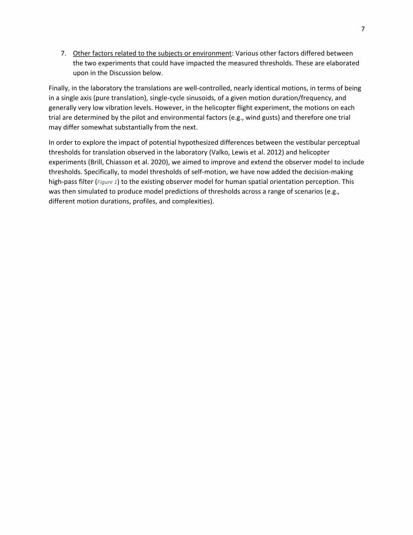
Adding decision-making and thresholds to the observer model

In order to add the decision-making dynamics of Figure 1 to the existing observer model for human

spatial orientation, we focused on just the vestibular pathways of the model (observer includes visual

pathways, as well as proposed pathways of somatosensory and other orientation cues, such as 3D

audio, but these were not activated in our simulations). These pathways are shown in Figure 4 and are

reviewed elsewhere (Clark, Newman et al. 2019). Shown in red in Figure 4 are the additions made to the

model for decision-making. Specifically, to the perception of angular velocity and the translation

perception pathways, we added a high-pass filter associated with decision-making. While here we focus

on vestibular perceptual thresholds for translation, these were also added to the angular velocity

perception pathway, such that rotation thresholds could be captured as well (e.g., “Did I rotate to the

left or to the right?”). A similar approach could be applied to the perception of gravity in order to

capture tilt thresholds (not shown in Figure 4 nor yet implemented).

Figure 4: Additions of decision-making and thresholds to the observer model for human spatial orientation perception. As shown in (Clark, Newman et al. 2019), the vestibular orientation model is after (Merfeld, Young et al. 1993) with updates from (Newman 2009). Bold denotes three-dimensional vectors. The model uses the standard head-fixed, right-handed coordinate system with X out the nose, Y out the left ear, and Z out the top of the head. Hat symbols correspond to brain estimates of that parameter. Body/world dynamics (pink) produce physical stimulation (𝒇 and 𝝎) to the otoliths (OTO) and semicircular canals (SCC, orange), yielding sensory afferent signals (𝜶𝑶𝑻𝑶 and 𝜶𝑺𝑪𝑪). The brain compares these with expected sensory afferent signals (�̂�𝑶𝑻𝑶 and �̂�𝑺𝑪𝑪). Vector differences (red circles) between actual and expected sensory afferent signals produce two sensory conflict signals (𝒆𝒂 and 𝒆𝝎). Similarly, 𝒆𝒇 represents the rotation vector error (direction and magnitude) required to

align the actual and expected otolith measurements (red box, see Merfeld, Young et al. 1993, Equations 15 and 16 for details). Sensory conflict signals are weighted by feedback gains (K’s, green) to produce central estimates (i.e., perceptions of), angular velocity, gravity, and linear acceleration. In Merfeld et al.’s (1993) implementation, the 𝒆𝝎 conflict signal was applied directly to the angular velocity estimate and not its rate of change, as in a formal Kalman filter approach. Merfeld et al. (1993) originally proposed four scalar feedback gains (Ka, Kf, Kfω, and Kω). Highlighted with a thick border, Newman (2009) subsequently added K1=Kω/(Kω+1) to ensure the closed loop gain for angular velocity was unity. Expected sensory afferent signals are produced using

internal models of the otoliths and semicircular canals (𝑂�̂�𝑂 and 𝑆�̂�𝐶, respectively, in purple) and internal models of body/world dynamics (light green). It is assumed the brain has learned internal models that match the physical dynamics well.

For example, the internal model of the semicircular canals (𝑆�̂�𝐶) has the same high pass filter transfer function as that of the physical canals (SCC). As part of this project, we have added those components in red. These include normally distributed sensory noise (N), with zero-mean and standard deviation σOTO and σSCC for the otoliths and semicircular canals, respectively.

9

Decision-making high-pass filtering is added to angular velocity perception and the translation perception pathways. For the translation perception decision-making, we assumed the decision-making was applied to the perception of linear velocity, which is produced through leaky integration of the perception of linear acceleration, added by (Newman 2009), and shown as dotted red lines. These yield a rotational decision variable (dω) and translational decision variable (dvel).

Notably, we applied the high-pass filter for decision-making along the translation pathway to the

perception of linear velocity (as opposed to directly to the perception of linear acceleration). The

perception of linear velocity is computed in the model by leaky integration of the perception of linear

velocity, an addition made by Newman (2009), and is shown as dotted red in Figure 4. In mathematics,

leaky integration is a specific differential equation that takes the integral of an input, but gradually leaks

a small amount of input over time. Finally, Gaussian white noise was added to the otolith and

semicircular canal sensory measurements. Sensory noise is presumably a primary limiting factor for

thresholds (i.e., why humans cannot reliably perceive infinitesimally small self-motions) and determines

an appropriate “decision boundary”. However, the simulations shown below were performed without

including sensory noise. Instead the decision boundary which the decision variable must reach to be

correctly perceived is set to match experimental threshold data. Future work should use the model

implementation to investigate the relationship between sensory noise, its effect on the decision

variable, and associated decision boundaries.

The computational model and additions, shown in Figure 4, were implemented in Matlab/Simulink

(2020a, Mathworks, Inc.).

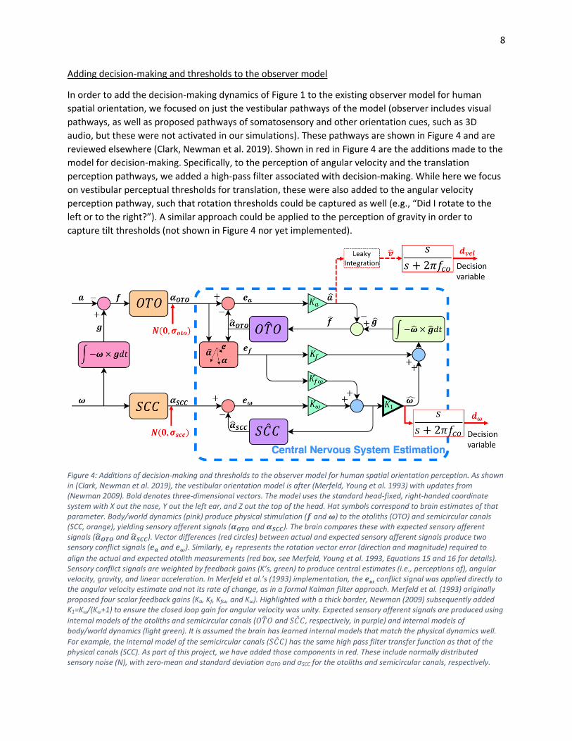
Simulating Thresholds to Single-Cycle Sinusoid Accelerations Across Frequencies (Difference #1):

We begin by simulating a single-cycle sinusoid of acceleration to predict thresholds across a range of

frequencies, including those not previously tested experimentally. Details can be found in the caption of

Figure 5, however there are two primary takeaways: 1) the model predicted thresholds (panel g shows

them in terms of peak linear velocity, while panel h shows maximum linear acceleration) mimic

laboratory experimental thresholds from (Valko, Lewis et al. 2012), and 2) when the model is simulated

at lower frequencies (<0.05 Hz) to better match the motion duration used in the helicopter experiment

(~20 seconds), the predicted thresholds do not mimic those observed (range is shown with dotted gray

lines in panel h). This suggests that the motion duration (and associated frequency) cannot fully explain

the elevated thresholds observed in the helicopter experiment. While the model predicts increased

thresholds at lower frequencies (particularly in terms of peak velocity—panel g), they are still not as

elevated as those observed in the helicopter experiment. Specifically, even at 0.03 Hz (corresponding to

a 33 second long motion) the model predicts the threshold to be approximately 65 cm/s or in terms

linear acceleration approximately 7 cm/s2. In contrast, the helicopter thresholds ranged from 60-200

cm/s2. Thus, the motion frequency/duration is likely a contributing factor but does not fully explain the

elevated thresholds in the helicopter experiment.

10

Figure 5: Simulated translation thresholds across a range of frequencies, as compared to laboratory and helicopter experimental thresholds. Panels a-d show a simulation for a 1 Hz single-cycle sinusoid. The actual motion in panels a-b are shown in orange, while observer’s predicted time course of the perception are in blue. In the example, the motion is fairly well perceived, though the perceived linear velocity is somewhat underestimated due to the leaky integration. For reference, panel c shows the otolith afferent neuron measurement (blue) and that expected by the CNS (orange). As in Figure 4, the perceived linear velocity is then processed by the decision-making high-pass filter to produce the linear velocity decision variable in panel d. The motion stimulus in this example (orange in panels a, b) is such that the decision variable (panel d) just reaches the decision boundary shown as a large red horizontal line in panel d. We set this decision boundary at approximately 0.25 (arbitrary units), such that the resulting thresholds matched laboratory experimental data (orange x’s in panels g-h). The simulation in panels a-d for 1 Hz, was repeated for 0.03, 0.05, 0.1, 0.3, 0.5, 2, and 5 Hz motions, and maximum values shown in panels e-f with the corresponding variables mapped across panels with black arrows. Panel e shows the maximum that the linear velocity perception reaches in each simulation (orange x’s, corresponding to the peak of the blue line in panel a) and the decision variable (blue o’s, found as the peak of the blue line in panel d), each normalized by the maximum of the actual linear velocity to depict a “gain”. As the frequency is reduced in panel e, the linear velocity perception gain decreases (due to the leaky integration from perception of linear acceleration), as does the decision variable gain to an even greater extent (due to the added decision-making high-pass filtering). Panel f shows the corresponding maximum linear acceleration (black line, corresponding to maximum of orange in panel b), perceived linear acceleration (orange o’s, maximum of blue in panel b), and otolith afferent response (OTO Afferent, yellow o’s, maximum of blue in panel c). Notably, for the fixed peak linear velocity in these simulations, the maximum linear acceleration (black) decreases with decreasing frequency. Relative to this, the otolith afferent response (yellow o’s) transduces well (though at frequencies >2 Hz, the otolith mechanics cannot respond quickly enough and the afferent response is reduced as compared to the acceleration stimulation). Despite the effective transduction, the perceived linear acceleration (orange o’s) is relatively reduced at lower frequencies (due to the very low frequency gravito-inertial stimulation being misperceived as tilt, instead of translation—tilt perception is not shown here). In panels g-h, the actual peak linear velocity and maximum linear acceleration (corresponding variables mapped across panels with gray arrows) were scaled and shown to identify those necessary for the decision variable in panel d to reach the fixed decision boundary. This corresponds to the “threshold” (i.e., the physical stimulus large enough to be correctly identified). The model simulation’s predicted threshold (blue o’s), shown in terms of peak linear velocity in panel g and maximum linear acceleration in panel h, are able to capture the laboratory thresholds from Valko et al. (2012) shown as orange x’s (note that the decision boundary—red line in panel d—was a free parameter adjusted to help match the data, but the efficacy in matching the thresholds across frequency is due to the decision-making high-pass filter). Most critically, the model predicted thresholds fail to match the range of helicopter thresholds (dotted gray horizontal lines in panel h), which are shown at the lower “frequencies” due to the motions used in that experiment typically being longer in duration.

11

Simulating Thresholds to Different Motion Profiles (Difference #2):

Next, we consider the effect of an asymmetric motion profile. Recall the standard laboratory motion

profile is a single-cycle sinusoid in which the acceleration and deceleration are symmetric and the peak

velocity is halfway through the motion (Figure 3). In contrast, the helicopter profiles tended to have a

shorter, large acceleration, followed by a longer deceleration period. To simulate this, we produced a

smooth asymmetric profile (Figure 6g-j) in which the peak linear velocity occurs only 20-30% into the

profile, as opposed to halfway. The resulting thresholds (Figure 6a-b) are predicted to differ between

the typical laboratory symmetric profile (blue o’s) and the asymmetric (yellow □’s). In particular, at

lower frequencies (0.03-0.05 Hz, corresponding to 33-20 seconds, similar to that used in the helicopter

experiment), the asymmetric profile actually has lower thresholds, both in terms of peak velocity (panel

a) and maximum acceleration (panel b). Thus the predicted thresholds for the asymmetric profile also do

not match those observed in the helicopter experiment. This suggests the asymmetry of the short, fast

acceleration is not the cause of the elevated thresholds from Brill et al. (2020).

Figure 6: Effect of an asymmetric motion profile on simulated thresholds. Panels a and b show the predicted thresholds in terms of peak linear velocity and maximum linear acceleration, similar to Figure 5g-h. Panels c-f show the example simulation for a 1Hz motion using the symmetric single-cycle sinusoid typically used in laboratory experiments (same as Figure 5a-d). Now, we also simulate an asymmetric motion profile (panels g-j) that includes a short, large acceleration (orange in panel h shows actual linear acceleration profile) followed by a longer deceleration period. The resulting peak linear velocity (orange in panel g) occurs between 0.2-0.3 seconds into the 1 second motion profile. The resulting predicted thresholds of this asymmetric motion profile are shown as yellow □’s in panels a-b. While the thresholds for the asymmetric profile differ from that for the symmetric profile (blue o’s in panels a-b), they do not mimic the elevated threshold range observed in the helicopter experiment (gray dotted lines in panel b).

Simulating Thresholds to Full 6 Degree-of-freedom Helicopter Motion Profile (Difference #3):

Finally, we performed simulations using an actual recorded motion profile from one example trial of Brill

et al. (2020)’s helicopter experiment. This is a full six degree-of-freedom profile, such that when

translating to the left, there is also roll tilt to the left and then to the right (during deceleration), as well

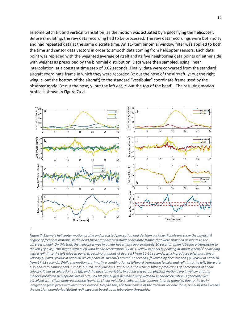
12

as some pitch tilt and vertical translation, as the motion was actuated by a pilot flying the helicopter.

Before simulating, the raw data recording had to be processed. The raw data recordings were both noisy

and had repeated data at the same discrete time. An 11-item binomial window filter was applied to both

the time and sensor data vectors in order to smooth data coming from helicopter sensors. Each data

point was replaced with the weighted average of itself and its five neighboring data points on either side

with weights as prescribed by the binomial distribution. Data were then sampled, using linear

interpolation, at a constant time step of 0.02 seconds. Finally, data were converted from the standard

aircraft coordinate frame in which they were recorded (x: out the nose of the aircraft, y: out the right

wing, z: out the bottom of the aircraft) to the standard “vestibular” coordinate frame used by the

observer model (x: out the nose, y: out the left ear, z: out the top of the head). The resulting motion

profile is shown in Figure 7a-d.

Figure 7: Example helicopter motion profile and predicted perception and decision variable. Panels a-d show the physical 6 degree of freedom motions, in the head-fixed standard vestibular coordinate frame, that were provided as inputs to the observer model. On this trial, the helicopter was in a near hover until approximately 10 seconds when it began a translation to the left (+y axis). This began with a leftward linear acceleration (+y axis, yellow in panel b, peaking at about 20 cm/s2 coinciding with a roll tilt to the left (blue in panel d, peaking at about -8 degrees) from 10-15 seconds, which produces a leftward linear velocity (+y axis, yellow in panel a) which peaks at 340 cm/s around 17 seconds, followed by deceleration (-y, yellow in panel b) from 17-23 seconds. While the motion is primarily a combination of leftward translation (y axis) and roll tilt to the left, there are also non-zero components in the x, z, pitch, and yaw axes. Panels e-h show the resulting predictions of perceptions of linear velocity, linear acceleration, roll tilt, and the decision variable. In panels e-g actual physical motions are in yellow and the model’s predicted perceptions are in red. Roll tilt (panel g) is perceived very well and linear acceleration is generally well perceived with slight underestimation (panel f). Linear velocity is substantially underestimated (panel e) due to the leaky integration from perceived linear acceleration. Despite this, the time course of the decision variable (blue, panel h) well exceeds the decision boundaries (dotted red) expected based upon laboratory thresholds.

13

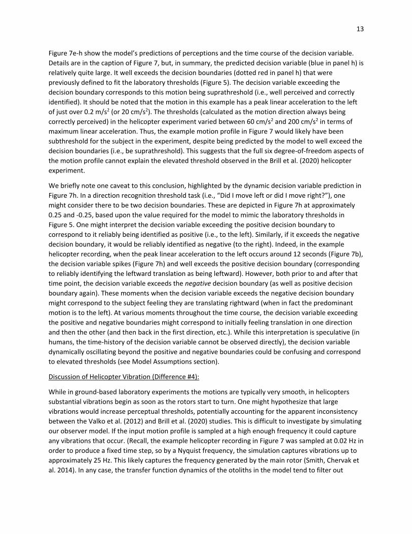
Figure 7e-h show the model’s predictions of perceptions and the time course of the decision variable.

Details are in the caption of Figure 7, but, in summary, the predicted decision variable (blue in panel h) is

relatively quite large. It well exceeds the decision boundaries (dotted red in panel h) that were

previously defined to fit the laboratory thresholds (Figure 5). The decision variable exceeding the

decision boundary corresponds to this motion being suprathreshold (i.e., well perceived and correctly

identified). It should be noted that the motion in this example has a peak linear acceleration to the left

of just over 0.2 m/s2 (or 20 cm/s2). The thresholds (calculated as the motion direction always being

correctly perceived) in the helicopter experiment varied between 60 cm/s2 and 200 cm/s2 in terms of

maximum linear acceleration. Thus, the example motion profile in Figure 7 would likely have been

subthreshold for the subject in the experiment, despite being predicted by the model to well exceed the

decision boundaries (i.e., be suprathreshold). This suggests that the full six degree-of-freedom aspects of

the motion profile cannot explain the elevated threshold observed in the Brill et al. (2020) helicopter

experiment.

We briefly note one caveat to this conclusion, highlighted by the dynamic decision variable prediction in

Figure 7h. In a direction recognition threshold task (i.e., “Did I move left or did I move right?”), one

might consider there to be two decision boundaries. These are depicted in Figure 7h at approximately

0.25 and -0.25, based upon the value required for the model to mimic the laboratory thresholds in

Figure 5. One might interpret the decision variable exceeding the positive decision boundary to

correspond to it reliably being identified as positive (i.e., to the left). Similarly, if it exceeds the negative

decision boundary, it would be reliably identified as negative (to the right). Indeed, in the example

helicopter recording, when the peak linear acceleration to the left occurs around 12 seconds (Figure 7b),

the decision variable spikes (Figure 7h) and well exceeds the positive decision boundary (corresponding

to reliably identifying the leftward translation as being leftward). However, both prior to and after that

time point, the decision variable exceeds the negative decision boundary (as well as positive decision

boundary again). These moments when the decision variable exceeds the negative decision boundary

might correspond to the subject feeling they are translating rightward (when in fact the predominant

motion is to the left). At various moments throughout the time course, the decision variable exceeding

the positive and negative boundaries might correspond to initially feeling translation in one direction

and then the other (and then back in the first direction, etc.). While this interpretation is speculative (in

humans, the time-history of the decision variable cannot be observed directly), the decision variable

dynamically oscillating beyond the positive and negative boundaries could be confusing and correspond

to elevated thresholds (see Model Assumptions section).

Discussion of Helicopter Vibration (Difference #4):

While in ground-based laboratory experiments the motions are typically very smooth, in helicopters

substantial vibrations begin as soon as the rotors start to turn. One might hypothesize that large

vibrations would increase perceptual thresholds, potentially accounting for the apparent inconsistency

between the Valko et al. (2012) and Brill et al. (2020) studies. This is difficult to investigate by simulating

our observer model. If the input motion profile is sampled at a high enough frequency it could capture

any vibrations that occur. (Recall, the example helicopter recording in Figure 7 was sampled at 0.02 Hz in

order to produce a fixed time step, so by a Nyquist frequency, the simulation captures vibrations up to

approximately 25 Hz. This likely captures the frequency generated by the main rotor (Smith, Chervak et

al. 2014). In any case, the transfer function dynamics of the otoliths in the model tend to filter out

14

stimulation >10 Hz, such that including higher frequency vibrations in the inputs file would likely not

impact the observer model predictions of perception or the decision variable.

Instead, we may expect that a high vibration environment would impact where the decision boundaries

are set. In particular, if there are large vibrations it would be logical to set the decision boundaries wider

to avoid identifying the direction of motion based just upon the vibrations. If subjects use this

decision-making strategy (likely subconsciously), we would expect a much higher threshold (i.e., a larger

motion is required to reach the wider decision boundaries and be reliably identified). While this

reasoning is speculative, it could potentially explain the elevated thresholds observed in the helicopter

experiment.

Discussion of Different Tasks and Definition/Calculation of Thresholds (Differences #5-6):

In Difference #5, we note that laboratory threshold experiments typically employ a forced-choice

decision (“Did I move left or right?”) made after the motion is complete. In the helicopter experiment

subjects continuously reported their perception of the motion verbally and using hand motions. The

difference in psychophysical task may produce differences in the resulting threshold. Arguably, the task

used in the helicopter is more of a continuous perceptual reporting task and does not require the same

type of binary decision required in forced-choice threshold tasks. This may affect the resulting data,

since the brain appears to use additional processing (i.e., filtering) when making a decision (Merfeld,

Clark et al. 2016) compared to producing a continuous perception of motion. Exactly how this affects the

computed threshold values remains uncertain.

As noted earlier (Difference #6), laboratory thresholds are typically computed by fitting a psychometric

curve, often a cumulative Gaussian from which the “1-sigma” threshold can be defined which

corresponds to the stimulus magnitude at which 84.1% of trials would be correctly identified. In the

helicopter experiment the threshold was defined as the smallest stimulus magnitude in which the

subject was always able to correctly identify the motion direction across approximately 40 trials

(personal communication, A. Rupert regarding (Brill, Chiasson et al. 2020)). The difference in definition

obscures a direct comparison between threshold values between (Brill, Chiasson et al. 2020) and (Valko,

Lewis et al. 2012). In any case, the definition of 100% correct over 40 trials would be expected to

produce a larger (potentially much larger) threshold, as compared to the 1-sigma definition

(corresponding to 84.1% correct).

Further, in the helicopter experiment the motions were produced by the pilot and thus not identical

across trials. For example, two trials with a similar maximum linear acceleration to the left could occur

over different durations, have different linear acceleration/velocity profiles, and have different

amounts/presence of concurrent roll and pitch tilt and vertical and fore-aft translation. Motions that

differ in these other aspects, but are considered the “same” in terms of maximum linear acceleration for

the purpose of analysis are likely to make the computed threshold larger. These factors likely contribute

to the elevated threshold values observed in the helicopter experiment, though it is difficult to quantify

the magnitude of the contribution. While speculative, we believe the different definitions are not the

lone contributor to the roughly 10x difference in threshold values between studies.

15

Discussion of Other Factors and Future Experiments (Difference #7):

There were several other differences between the Brill et al. (2020) helicopter experiment and those

typical of laboratory threshold experiments that are worth noting as potential factors in the resulting

thresholds. For example, subjects in the helicopter flight experiment were pilots, while those in

laboratory experiments are typically non-pilots. The different motion experiences of pilots may impact

how they perceive motions (Tribukait, Gronkvist et al. 2011). The ages of the two groups differ, with

those in the helicopter study being older than those in most lab experiments, and vestibular perceptual

thresholds increase with age over 40 years (Bermudez Rey, Clark et al. 2016). In the laboratory

experiments, such as Valko et al. (2012), subjects are instructed that motions are pure translations, to

either the left or right and the motion frequency is blocked so the subject knows the duration. In the

helicopter experiment there was more realistic uncertainty of what types of motions were possible and

these expectations (or lack thereof) may influence motion perception and thresholds. Finally, in the

helicopter experiment, the temperature was typically hot and some subjects experienced motion

sickness. In laboratory testing, the room temperature is controlled and tests are usually stopped if the

subject reports motion sickness. While there has not been a systematic investigation of these factors on

vestibular perceptual thresholds, one might hypothesize distracting factors (uncomfortably hot, motion

sickness) could lead to elevated thresholds.

Summary of Conclusions and Proposed Future Investigations:

Using a computational model of human orientation perception and now decision-making dynamics, we

were able to explore potential explanations for the elevated thresholds observed in the helicopter

experiment. While we have not reached a definitive explanation, we have ruled out some alternatives as

unlikely and now propose future investigations to delineate between the remaining potential

contributors.

We added a high-pass filter decision-making element to the observer model for spatial orientation

perception and defined a decision boundary that reasonably predicts translational thresholds across a

range of frequencies (0.3, 0.5, 1, 2, 5 Hz) observed in a laboratory experiment (Valko, Lewis et al. 2012).

We then simulated that model with a fixed decision boundary, using lower frequency (i.e., longer

duration) motions to assess whether the longer duration of the helicopter motions could explain the

higher thresholds observed. While thresholds were predicted to be higher for lower frequencies, they

were not predicted to be as high as observed in the helicopter experiment, ruling out motion duration

(Difference #1) as the lone contributor, though it is likely to contribute. Next, we simulated profiles that

were asymmetric (short, large acceleration followed by a longer deceleration) and similar to those used

in the helicopter experiment. This also affected the predicted thresholds, but not in a manner consistent

with the helicopter data and thus was ruled out (Difference #2). Finally, we simulated an example profile

recording from the helicopter experiment, including full six degree of freedom motions (i.e., during a

translation to the left, there was concurrent roll tilt, as well as slight pitch tilts and out-of-axis

translations). While the example profile had a maximum acceleration of ~20 cm/s2, which was below the

thresholds observed in the helicopter experiment (60-200 cm/s2 across subjects), the model predicted

the decision variable to exceed the decision boundaries (defined to capture the thresholds from Valko et

al., 2012). This suggests the six degree of freedom motions are not the cause of elevated thresholds in

the helicopter experiment (Difference #3). However, in this simulation the decision variable exceeded

both the positive and negative boundaries at different time points, which could be interpreted as being

16

suprathreshold, but confusing and disorienting to the subject such that they may not reliably identify

the direction. We conclude the dynamics of the decision variable warrant more investigation.

We then qualitatively discuss the potential impact of different psychophysical tasks (Difference #4),

definitions/computations of threshold (Differences #5&6) and various other factors (Difference #7). It is

difficult to quantify the exact impact of these, but the different definition of thresholds likely caused the

computed helicopter thresholds to be higher than they would be if defined using the “1-sigma”

definition. We suggest this is a contributing factor, but it likely does not explain the roughly 10x

difference in computed thresholds between investigations.

The findings using the computational model simulations suggest critical future experimental

investigations. First, human vestibular perceptual thresholds in translation should be quantified across a

broader range of frequencies, particularly lower frequencies relative for various helicopter and fixed-

wing maneuvers, using standard laboratory methods. To our knowledge, the most exhaustive

investigation (Valko, Lewis et al. 2012) has only investigated motions of 0.3-5 Hz (0.2-3.33 seconds in

duration). Investigating lower frequencies (longer durations) has historically been limited by the large

displacements required which exceed the capabilities of typical Moog/hexapod platforms. Tilt

thresholds have been shown to vary across a range of frequencies (Karmali, Lim et al. 2014, Lim, Karmali

et al. 2017), rotational thresholds are known to increase at lower frequencies (Grabherr, Nicoucar et al.

2008), and our improved computational model predicts translation thresholds will also increase (Figure

5g). Attempts at quantifying tilt thresholds at 0.02 and 0.01 Hz (50 and 100 second long motions)

suggested subjects may struggle to maintain focus/attention for frequencies lower than ~0.05 Hz,

producing subject lapses that contaminate the data. Effectively extrapolating the model predictions

suggest the lower frequency is not the lone cause of the elevated helicopter thresholds, but these

predictions have not yet been validated. A few modern motion devices, including NAMRU-D’s

Disorientation Research Device or CU-Boulder Tilt-Translation Sled, have enhanced translation

capabilities that enable quantifying translation thresholds at lower frequencies.

In addition to the typical forced-choice task following the motion, we suggest dynamics of perception

(and ideally the decision variable) during the motion be investigated. Several of our simulations suggest

that even when the motion is unidirectional, the perception of linear velocity and decision variable may

include peaks in both the motion direction and opposite to it, a confusion that exemplifies spatial

disorientation. This is most pronounced for the simulation of the six degree-of-freedom helicopter

motion (Figure 7e,h), but can also be observed for pure single-cycle sinusoids in translation (Figure 5a,d).

A continuous perceptual task, even just continuously reporting the direction of perceived translation

velocity, could determine if there is, indeed, bidirectional perception in response to unidirectional

translations. Particularly for small motions, it may be appropriate to allow the subject to respond

continuously with three options: moving left, moving right, or uncertain. Assessing the dynamics of the

decision variable is more difficult, since, presumably, it can only be queried by requiring a decision.

Varied motion profiles and/or time-to-detect tasks (i.e., where the subject responds as soon as they can

tell which direction they are translating) may be used to assess the dynamics of the decision variable.

A ground-based study could also be performed to investigate the effect of vibrations on translation

thresholds (e.g., using a shaker table within a motion device). As discussed above, we might hypothesize

that a vibration environment may cause an increase in the decision boundaries, effectively increasing

the resulting direction-recognition threshold. Experimental threshold data at varying vibration levels,

17

combined with simulations of the computational model could be used to tease apart the contribution of

vibration to translation thresholds in-flight. As well as vibrations, thresholds should be assessed when

the translation is combined with a concurrent tilt. This coupled motion is common in helicopters and

would be expected to impact translation perception (i.e., tilt vs. translation disambiguation), particularly

at lower frequencies. Further, there is evidence (Macauda, Ellis et al. 2019) that when additional

motions (e.g., rotations) precede the translation, it affects the threshold translation perception. These

“self-motion after-effects” are not well understood and should be further investigated. The example

simulation of the six degree-of-freedom helicopter motion (Figure 7), does not appear to fully explain

the elevated thresholds, but to our knowledge translation thresholds have not be quantified when the

motions are paired with tilts.

Similarly, a ground-based experiment could compare the thresholds computed using the typical

laboratory two-alternative forced-choice task and the cumulative Gaussian psychometric curve with

those used in the Brill et al. (2020) helicopter experiment (i.e., the continuous verbal and hand reporting

and identifying the motion required to always be correctly perceived/identified). A laboratory

investigation of these effects would allow for repeated, well-controlled motion profiles. Probabilistic

simulations of an underlying psychometric curve (Karmali, Chaudhuri et al. 2016), with a finite number

of trials (e.g., the 40 trials used in the helicopter experiment), could be used to define a conversion

between the 1-sigma threshold (84.1% correct) and the stimulus expected to produce no incorrect

outcomes over the 40 trials. While it would not require any experimentation, this effort would require

an approximation of how the stimulus magnitudes were selected during the helicopter experiment.

Finally, there are several other factors which were present during the helicopter experiment (and

common during flight) which have not been studied in terms of their effects upon thresholds. For

example, pilots perceive some motions differently (Tribukait, Gronkvist et al. 2011), but it is unknown if

thresholds differ between pilots and non-pilots. In flight, environmental conditions (e.g., turbulence or

wind gusts) commonly cause unpredictable motions in different axes, while in laboratory threshold

experiments subjects are instructed that motions are pure and unidirectional. The impact of uncertainty

about motion axis and duration should be investigated by randomly interleaving trials during testing, as

opposed to presenting them in blocks. Other factors that are common during flight, such as altered

temperature or motion sickness, could also be investigated in a controlled laboratory experiment. Lastly,

during flight pilots have divided attention across multiple tasks in addition to orientation perception.

Typically, in experiments quantifying thresholds subjects are exclusively tasked with focusing on their

own self-motion. The effect of divided attention on vestibular perceptual thresholds could be assessed

experimentally using a relevant secondary task. While each of these could be explored in a flight

experiment, we suggest they could be isolated and investigated at less cost in a series of ground-based

laboratory experiments, to identify the cause(s) of elevated translation thresholds observed by Brill et al.

(2020).

Model Assumptions:

As our main contribution, we added a decision-making element to improve the existing observer model

for orientation perception. In doing so, we applied several modeling assumptions, many of which were

detailed throughout. However, we would like to summarize a few of the key assumptions here and

suggest approaches to validate these assumptions.

18

First, we assumed that for translation thresholds, the decision-making high-pass filter was applied to the

perceived linear velocity signal within the observer model. This is motivated by subjects typically

producing a perception of linear velocity (as opposed to acceleration) when tasked with reporting

sensations of translation motions. Further, as in Newman (2009), we assumed the perception of linear

velocity to be computed via leaky integration of the perceived acceleration signal in the model. There is

some evidence (see Table 1 in (Clark, Newman et al. 2019)) that for large, lower frequency translation

humans imperfectly perceive linear velocity, consistent with leaky integration. However, these

assumptions (in parallel to alternative approaches) should be evaluated by empirically quantifying

thresholds at lower frequencies.

Second, in our implementation the decision-making high-pass filter process produces a time history of

the decision variable during a simulated motion profile. We have assumed that if the peak of this

decision variable (whenever that occurs during the profile) exceeds a fixed decision boundary, then it

would correspond to being suprathreshold or correctly identified. Such an approach contrasts the

concept of “evidence accumulation” in which information is accumulated throughout the stimulation

period. Our current “peak decision variable” assumption has a peculiar prediction in that the motion

profile and associated decision variable response are irrelevant once that peak has occurred. This

peculiarity becomes evident only when considering 1) the decision variable to have a time history and 2)

the stimulus (i.e., physical motion) and associated perceptions to vary over time. Item #1 is typically

ignored in standard signal detection theory (Green and Swets 1966) in which the decision variable is

stationary for a given trial. Item #2 is typically ignored for other (non-vestibular) threshold tasks in which

the stimulus is fixed and thus the evidence accumulation is assumed to be constant. While modeling

vestibular perceptual thresholds for translation requires making these assumptions, it also offers an

opportunity, through empirical assessment, to better understand decision-making dynamics related to

thresholds. In doing so, this will help identify when pilots may misperceive their direction of motion and

enter into a dangerous state of spatial disorientation.

19

References:

Benson, A. J. (1978). Spatial Disorientation - General Aspects. In J. Ernsting, A. N. Nicholson & D. J. Rainford (Eds.), Aviation Medicine (3rd ed., pp. 419-436). Butterworth Heinemann.

Benson, A. J., Hutt, E. C. B., & Brown, S. F. (1989). Thresholds for the Perception of Whole-Body Angular

Movement About a Vertical Axis. Aviation Space and Environmental Medicine, 60(3), 205-213. Benson, A. J., Spencer, M. B., & Stott, J. R. R. (1986). Thresholds for the Detection of the Direction of

Whole-Body, Linear Movement in the Horizontal Plane. Aviation Space and Environmental Medicine, 57(11), 1088-1096.

Bermudez Rey, M. C., Clark, T. K., Wang, W., Leeder, T., Bian, Y., & Merfeld, D. M. (2016). Vestibular

Perceptual Thresholds Increase Above the Age of 40. Frontiers in Neurology, 7(1), 162. Boeing. (2019). Fatalities by CICTT Aviation Occurrence Categories.

http://www.boeing.com/news/techissues/pdf/statsum.pdf. Brill, J. C., Chiasson, J., Kelley, A., Lawson, B., King, M., Basso, J., Chiaramonte, J., Harris, C., & A. H.

Rupert (2020). Perceptual Threshold of Linear Acceleration in Helicopters Applied to Modeling of Spatial Orientation Mishaps. Warfighter Performance Group.

Chaudhuri, S. E., Karmali, F., & Merfeld, D. M. (2013). Whole body motion-detection tasks can yield

much lower thresholds than direction-recognition tasks: Implications for the role of vibration. Journal of Neurophysiology, 110(12), 2764-2772.

Clark, T. K., Newman, M. C., Karmali, F., Oman, C. M., & Merfeld, D. M. (2019). Mathematical Models for

Dynamic, Multisensory Spatial Orientation Perception. Progress in Brain Research, 248, 65-90. Grabherr, L., Nicoucar, K., Mast, F. W., & Merfeld, D. M. (2008). Vestibular thresholds for yaw rotation

about an earth-vertical axis as a function of frequency. Experimental Brain Research, 186(4), 677-681.

Green, D. M. & Swets, J. A. (1966). Signal Detection Theory and Psychophysics. John Wiley and Sons, Inc. Karmali, F., Chaudhuri, S. E., Yi, Y., & Merfeld, D. M. (2016). Determining Thresholds using Adaptive

Procedures and Psychometric Fits: Evaluating Efficiency using Theory, Simulations, and Human Experiments. Experimental Brain Research, 234, 773-789.

Karmali, F., Lim, K., & Merfeld, D. M. (2014). Visual and vestibular perceptual thresholds each

demonstrate better precision at specific frequencies and also exhibit optimal integration. Journal of Neurophysiology, 111(12), 2393-2403.

Lim, K., Karmali, F., Nicoucar, K., & Merfeld, D. M. (2017). Perception precision of passive body tilt is

consistent with statistically optimal cue integration. Journal of Neurophysiology, 117(5), 2037-2052.

20

Macauda, G., Ellis, A. W., Grabherr, L., Di Francesco, R. B., & Mast, F. W. (2019). Canal-otolith interactions alter the perception of self-motion direction. Atten Percept Psychophys, 81(5), 1698-1714.

MacNeilage, P. R., Ganesan, N., & Angelaki, D. E. (2008). Computational Approaches to Spatial

Orientation: From Transfer Functions to Dynamic Bayesian Inference. Journal of Neurophysiology, 100(6), 2981-2996.

Merfeld, D. M., Clark, T. K., Lu, Y. M., & Karmali, F. (2016). Dynamics of Individual Perceptual Decisions.

Journal of Neurophysiology, 115(1): 39-59. Merfeld, D. M., Young, L. R., Oman, C. M., & Shelhammer, M. J. (1993). A Multidimensional Model of the

Effect of Gravity on the Spatial Orientation of the Monkey. Journal of Vestibular Research, 3(2), 141-161.

Newman, M. C. (2009). A Multisensory Observer Model for Human Spatial Orientation Perception.

[Graduate thesis, Massachusetts Institute of Technology]. Newman, R. L., & Rupert, A. H. (2020). The Magnitude of the Spatial Disorientation Problem in Transport

Airplanes. Aerospace Medicine and Human Performance, 91(2), 65-70. Smith, S. D., Chervak, S. G., & Steinhauser, B. (2014). Vibration Characterization and Health Risk

Assessment of the Vermont Army National Guard UH-72 Lakota and HH-60M Medevac. Air Force Research Laboratory 711 Human Performance Wing.

Tribukait, A., Gronkvist, M., & Eiken O. (2011). The Perception of Roll Tilt in Pilots During a Simulated Coordinated Turn in a Gondola Centrifuge. Aviation Space and Environmental Medicine, 82(5), 523-530.

Valko, Y., Lewis, R. F., Priesol, A. J., & Merfeld, D. M. (2012). Vestibular Labyrinth Contributions to

Human Whole-Body Motion Discrimination. Journal of Neuroscience, 32(39), 13537-13542. Williams, H. P., Horning, D. S., Lawson, B. D., Powell, C. R., & Patterson, F. R. (2018). Effects of Various

Types of Cockpit Workload on Incidence of Spatial Disorientation in Simulated Flight. NAMRU-D.