Master Science Thesis Extending SU 2 to Aeroelastic Simulations using MpCCI Manuel Cellarius B.Sc. Supervised by: Dr. Simão Marques School of Mechanical and Aerospace Engineering Stranmillis Road Belfast BT9 5AH Univ.-Prof. Dr.-Ing. Wolfgang Schröder Dr.-Ing. Andreas Henze Chair of Fluid Mechanics and Institute of Aerodynamics Aachen Wüllnerstraße 5a 52062 Aachen October 2013

Welcome message from author
This document is posted to help you gain knowledge. Please leave a comment to let me know what you think about it! Share it to your friends and learn new things together.
Transcript

Master Science Thesis
Extending SU2 to Aeroelastic Simulations
using MpCCI
Manuel Cellarius B.Sc.
Supervised by:
Dr. Simão Marques
School of Mechanical and
Aerospace Engineering
Stranmillis Road
Belfast BT9 5AH
Univ.-Prof. Dr.-Ing. Wolfgang Schröder
Dr.-Ing. Andreas Henze
Chair of Fluid Mechanics and Institute of
Aerodynamics Aachen
Wüllnerstraße 5a
52062 Aachen
October 2013
Contents
1. Introduction 1
2. Coupling Foundation 2
2.1. Transformation Methods . . . . . . . . . . . . . . . . . . . . . . . . . . . . . . . . . . 3
2.1.1. Requirements . . . . . . . . . . . . . . . . . . . . . . . . . . . . . . . . . . . . 3
2.1.2. Infinite Plate Spline . . . . . . . . . . . . . . . . . . . . . . . . . . . . . . . . 4
2.1.3. Finite Plate Spline . . . . . . . . . . . . . . . . . . . . . . . . . . . . . . . . . 5
2.1.4. Boundary Element Method . . . . . . . . . . . . . . . . . . . . . . . . . . . . 6
2.1.5. Radial Basis Function . . . . . . . . . . . . . . . . . . . . . . . . . . . . . . . 6
2.1.6. Constant Volume Tetrahedron . . . . . . . . . . . . . . . . . . . . . . . . . . 8
2.2. Mesh Deformation Methods . . . . . . . . . . . . . . . . . . . . . . . . . . . . . . . . 9
2.2.1. Spring Analogy Method . . . . . . . . . . . . . . . . . . . . . . . . . . . . . . 9
2.2.2. Stabilisation Techniques . . . . . . . . . . . . . . . . . . . . . . . . . . . . . . 10
2.3. Multiphysics Code Coupling Interfaces - MpCCI . . . . . . . . . . . . . . . . . . . . 12
2.3.1. Transformation Method . . . . . . . . . . . . . . . . . . . . . . . . . . . . . . 13
2.3.2. Coupling Algorithm . . . . . . . . . . . . . . . . . . . . . . . . . . . . . . . . 14
3. MpCCI Application Programming Interface 16
3.1. GUI and Perl Script Integration . . . . . . . . . . . . . . . . . . . . . . . . . . . . . . 17
3.1.1. GUI Configuration File . . . . . . . . . . . . . . . . . . . . . . . . . . . . . . 17
3.1.2. Perl Scripts . . . . . . . . . . . . . . . . . . . . . . . . . . . . . . . . . . . . . 19
3.2. Code Adapter Integration . . . . . . . . . . . . . . . . . . . . . . . . . . . . . . . . . 21
3.2.1. Code Structure of SU2 . . . . . . . . . . . . . . . . . . . . . . . . . . . . . . . 22
3.2.2. Coupling Strategy . . . . . . . . . . . . . . . . . . . . . . . . . . . . . . . . . 25
3.2.3. Code Adapter Implementation . . . . . . . . . . . . . . . . . . . . . . . . . . 28
4. Validation 49
4.1. Vortex-Induced Vibration of a Thin-Walled Structure . . . . . . . . . . . . . . . . . 49
4.1.1. Variation of Reynolds Number . . . . . . . . . . . . . . . . . . . . . . . . . . 53
4.1.2. Variation of Mass . . . . . . . . . . . . . . . . . . . . . . . . . . . . . . . . . . 55
4.2. Elastic Flap in a Duct . . . . . . . . . . . . . . . . . . . . . . . . . . . . . . . . . . . 57
4.3. Mesh Deformation . . . . . . . . . . . . . . . . . . . . . . . . . . . . . . . . . . . . . 61
5. Summary and Outlook 62
Bibliography 63
i

Nomenclature
List of Figures 66
A. Appendix 68
B. Instruction for Code Adapter Integration 70
B.1. Adapt the C++ Files . . . . . . . . . . . . . . . . . . . . . . . . . . . . . . . . . . . . 70
B.2. Adapt the Make Files . . . . . . . . . . . . . . . . . . . . . . . . . . . . . . . . . . . 73
B.3. Adapt MpCCI . . . . . . . . . . . . . . . . . . . . . . . . . . . . . . . . . . . . . . . 74
ii

Nomenclature
Latin Symbols
Acronym Definition
API Application programming interfaceBC Boundary conditionCFD Computational fluid dynamicsCGNS CFD general notation systemFEM Finite element methodFSI Fluid-structure interactionGUI Graphical user interfaceMpCCI Multiphysics Code Coupling InterfacesNS Navier-StokesRe Reynolds numberRANS Reynolds averaged Navier-StokesSt Strouhal numberSU2 Stanford University Unstructred
Latin Symbols
Symbol Definition
A Aread DistanceE Young’s modulusf FrequencyF ForceK Stiffness matrixk StiffnessL LengthM Moment~n Normal vectorp Pressurer Distancet TimeT Linear transformation matrixu DisplacementV Volumev Velocity
iii

Nomenclature
Greek Symbols
Symbol Definition
δW Virtual workϕ Phase angleφ Basis functionµ Dynamic viscosityν Poisson’s ratioρ Densityτ Viscous shear stress tensor
Subscripts and superscripts
Symbol Definition
a Aerodynamic gridE Edgeip Interpolantn Normalorg Originalrel relatives Structural grid, source mesht Target mesh, tangential
iv

1. Introduction
In order to perform aeroelastic simulations a robust coupling between CFD and FEM grids is
necessary e.g. considering transonic flow problems; the solution is gained and evaluated from
this excursion. The Fraunhofer Institute for Algorithms and Scientific Computing, SCAI, has
developed MpCCI. MpCCI is an application independent interface for the coupling of different
simulation codes by way of, but not limited to, calculating mesh neighborhoods and interpolating
physical quantity values. The aforementioned software has been used thus far successfully to couple
the CFD solver Fluent with the FEM solver Nastran at the School of Mechanical and Aerospace
Engineering of The Queen’s University Belfast.
The aim of this work is to couple Nastran with the open-source CFD code SU2 developed at the
Aerospace Design Laboratory at Stanford University using MpCCI. To accomplish this, the appli-
cation programming interface of MpCCI will be used to develop a code in C++ and C for coupling
SU2 with MpCCI. SU2 has, incorporated within its design, the feature of deformable models and
grids and therefore is particularly suitable for aeroelastic investigations. Furthermore, its capability
of computing adjoint solutions gives this framework the potential to solve multi-disciplinary design
optimisation problems.
As the coupling is the main topic of this work, different transformation methods are explained in
chapter 2 as well as mesh deformation methods and an overview about the capabilities of MpCCI.
In chapter 3 the integration of the communication between SU2 and MpCCI is described. Therefore
the code structure of SU2 is explained briefly. Before the implementation of the code adapter is
explained in detail, the coupling strategy is described. The implementation is validated with two
test cases in chapter 4. In the first the vortex-induced vibration of a two dimensional thin-walled
structure is analysed. The oscillation of an elastic flap in a three dimensional duct is investigated
in the second. Both cases are simulated with SU2 and Fluent in a coupled simulation with Nastran
using MpCCI.
1

2. Coupling Foundation
Computational aeroelasticity investigation is based on the coupling of Computational Fluid Dy-
namics (CFD) and Computational Structure Dynamics (CSD) dynamics. Two different strategies
are distinguished to solve this problem: the monolithic and the partitioned approach.
The first combines the fluid and structural equations in order to solve and simultaneously integrate
them in time, but requires a new solver and a new grid. In addition referring to Guruswamy and
Byun (1995) the combined system is more difficult to solve. Hübner et al. (2004) and Bendiksen
(2004) use a monolithic approach to fluid-structure interaction.
The purpose of the partitioned approach is the coupling of independent solvers for fluid and struc-
ture through the wetted surface of the structure, which is deformable. As shown in figure 2.1
quantities need to be exchanged between the two solvers. The pressure or force distribution, ob-
tained by the fluid solver, is transferred to the structural solver, which computes the deformation of
the structure. Using the new deformed geometry, the fluid solver computes the resulting pressure
field. Its advantage is the possibility to use existing solvers and grids.
SU2 MD Nastran
Pressure Distribution
Deformation of Coupled Structure
CFD Solver CSD Solver
Figure 2.1.: Typical cycle for partitioned approach
The difficulty in using the partitioned approach is caused by the different discretisations, which
will not generally coincide. In comparison to the CFD grid, the structural model is commonly
simplified and therefore coarser as it usually does not result in high error penalties. Whereas a
wing surface is modeled quite accurately in each section in the CFD domain, the structural model
may just cover the beam of the wing. To overcome the discrepancy between the two grids either
the CSD grid needs to be refined, which results in a longer computation time, or a transformation
method must be used in order to interpolate and exchange the quantities of interest. In this work
transformation methods are used to couple the grids, which are discussed in more detail in section
2.1. An example of the monolithic approach is given by Farhat et al. (2003), who use a detailed
structural model to predict aeroelastic parameters of an F-16 fighter.
Due to the displacements computed by the CSD solver, the CFD grid needs to be deformed so that
mesh deformation techniques are necessary, described in section 2.2. The chapter finishes with an
overview on the coupling software ’Multiphysics Code Coupling Interfaces’ (MpCCI by Fraunhofer
SCAI) used in this work is given in section 2.3.
2

2. Coupling Foundation
2.1. Transformation Methods
Referring to Swift (2011) transformation methods may be divided into local and global methods.
Whereas local methods have low memory requirements and just use local information of the grids
for the transformation, global methods have higher memory requirements and always produce a
smooth grid, as they use more than just local information about the grids. Requirements for
the mesh transformation are described in section 2.1.1. Commonly used methods are explicated
afterwards.
2.1.1. Requirements
There are some physical requirements for the transformation methods formulated by Rendall and
Allen (2008):
(i) Conservation of energy
(ii) Conservation of total force and momentum
(iii) Exact recovery of translation and rotation
(iv) Force and displacement association
Using the principles of virtual work, the conservation of energy is ensured. The virtual work δW
is defined as
δW = ~δusT
· ~Fs = ~δuaT
· ~Fa , (2.1)
where ~δu is the the virtual displacement of the grid points and ~F is the force vector. The subscript
s indicates the structural grid and a the aerodynamic grid. The linear transformation T maps the
structural displacements onto the aerodynamic displacements:
~δua = aT s ~δus . (2.2)
Combining equations 2.1 and 2.2 leads to
~Fs = aT sT ~Fa , (2.3)
which fulfills the global conservation of energy (i) regardless of the method used, Sadeghi et al.
(2004).
The conservation of force and moment (ii) may be written as
ns∑
1
~Fs
∣∣∣i
=na∑
1
~Fa
∣∣∣i
andns∑
1
~Ms
∣∣∣i
=na∑
1
~Ma
∣∣∣i
. (2.4)
Referring to Rendall and Allen (2008) exact force association is only possible in the case of identical
surface grids.
In the case of rigid body motion of the structural grid, the transferred displacements should lead
to the same motion of the aerodynamic surface grid so that the exact recovery of translation and
rotation (iii) is fulfilled.
3
2. Coupling Foundation
To achieve force and displacement association (iv) points, which coincide at the beginning of an
simulation must remain “attached” throughout the entire simulation. Although based on the in-
terpolation scheme other nodes of the aerodynamic grid may contribute a force to the coincided
node, just the force of the node itself has to be transferred to its attached node of the structural
grid, Rendall and Allen (2008).
In addition some weaker requirements are formulated by Sadeghi et al. (2004), Rampurawala (2006)
and Swift (2011) concerning:
· Smoothness
· Complex geometries
· Memory and CPU requirements
If the deformation of the structural grid is smooth, the aerodynamic grid should be smooth as well.
The transformation method should not produce surface distortions as they can result in unnatural
results like shock waves and premature flow separation. Additionally surface distortions may cause
the mesh deformation method to generate an unwanted folded CFD grid e.g. at the junction of
wing and fuselage. Also a smooth pressure distribution should result in a smooth load distribution
on the structural grid despite the occurrence of shock waves.
Complex geometries must not cause any holes in the grid. Regarding a good performance of the
aeroelastic simulation, the CPU time necessary for the transformation method should be small in
comparison to the CFD calculation. The memory usage should be reduced to a minimum amount
as the high fidelity analysis may include large CFD and CSD grids.
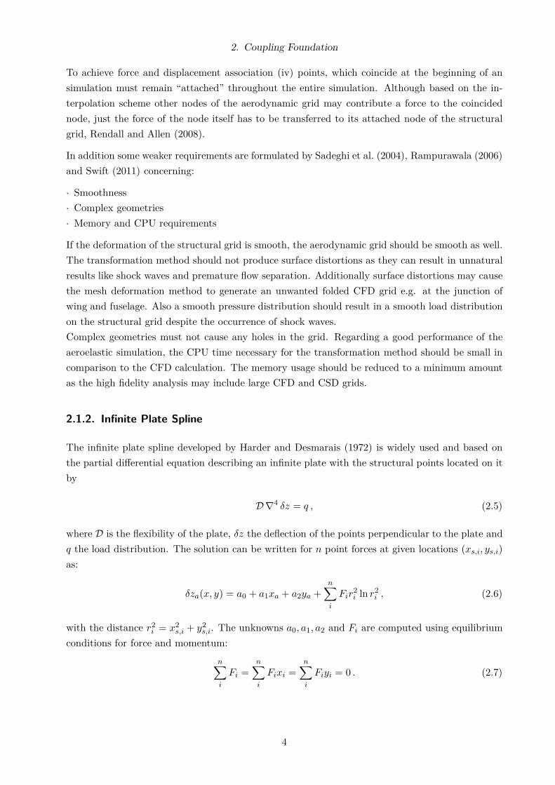
2.1.2. Infinite Plate Spline
The infinite plate spline developed by Harder and Desmarais (1972) is widely used and based on
the partial differential equation describing an infinite plate with the structural points located on it
by
D ∇4 δz = q , (2.5)
where D is the flexibility of the plate, δz the deflection of the points perpendicular to the plate and
q the load distribution. The solution can be written for n point forces at given locations (xs,i, ys,i)
as:
δza(x, y) = a0 + a1xa + a2ya +n∑
i
Fir2i ln r2
i , (2.6)
with the distance r2i = x2
s,i + y2s,i. The unknowns a0, a1, a2 and Fi are computed using equilibrium
conditions for force and momentum:
n∑
i
Fi =n∑
i
Fixi =n∑
i
Fiyi = 0 . (2.7)
4

2. Coupling Foundation
Given the deflection of the structural points, the distance between structural and aerodynamic
points can be computed using r2i = (xa,i − xs,i)
2 + (ya,i − ys,i)2 in order to solve for the deflection
of m aerodynamic points
δza,j(x, y) = a0 + a1xa,j + a2ya,j +n∑
i
Fir2i ln r2
i . (2.8)
It was assumed that all aerodynamic and structural points lie in the same plane. However, if that
is not the case they are projected onto a neutral plane. After computing the deflection the original
offset of the points is added to the result. The transformation matrix T according to transform
displacements and forces (equations 2.2 and 2.3) is derived in the appendix of Swift (2011).
As the infinite plate spline method is a global method, a large transformation matrix is generated,
which raises the memory usage. According to Swift (2011) the extrapolation from the interior
structural grid to the planform of the wing is not always reliable. Also this method is unable to
recover rigid rotation exactly, Goura (2001). In addition it is sensitive to the grid resolution and
its accuracy is poor in comparison, Smith et al. (1995).
2.1.3. Finite Plate Spline
Appa (1989) presented the finite plate spline method, which is based on a finite plate in comparison
to the infinite method presented in section 2.1.2. A virtual surface, lying between the aerodynamic
and structural grid, is generated and discretised into finite elements, which do not necessarily
need to coincide with either of the grids. Some constraints are applied in order to secure the
virtual surface passes through a sufficient number of structural points when the grid is deformed.
With the use of shape functions, displacements within the finite elements of the virtual surface
are calculated. Taking advantage of the shape functions, matrices for mapping displacements
from the virtual surface to the structural grid are derived sΨVS as from the virtual surface to the
aerodynamic grid aΨVS. The transformation matrix mapping the displacements from the structural
to the aerodynamic grid is given by
aT s = aΨVS(δ−1 K + sΨVST
sΨVS)−1
sΨVST
, (2.9)
with the stiffness matrix K and the penalty parameter δ. The full derivation of the transformation
matrix is presented in Appa (1989). The finite plate spline method was applied e.g. by Guruswamy
and Byun (1995) to a fighter aircraft wing. Smith et al. (1995) found out that the memory and
CPU usage is intensive due to the virtual surface.
5

2. Coupling Foundation
2.1.4. Boundary Element Method
Boundary
Elements
CSD grid
Elastic Homogenous Material
CFD grid !"#$% &'() *+, -$%.-/%0- 12 .0 .%$121!3-4% 513#/% 12 -4% -%-$.4%6$10 !7 "!5%0 89 : !;! <= ;&'&><+?#.-!10 &'&& "!5%7 . 010@3!0%.$ $%3.-!1074!A 8%-B%%0 -4% C#!6 .06 7-$# -#$.3 31 .-!107 B4! 4 .0 8% 3!0%.$!7%6 !0 -4% 7-$# -#$.3 6!7A3. %/%0-7 -1 "!5%Æ# !" : $Æ##!$ E%Æ##!% E&Æ##!& ;&'&F<$ : '!%!&% : #$ ! %"#;!<& : &$ E %"#; <" : $ ! G' $;(<%;(< ;&'&H<#;)< : !� I !(! ( (! I !("!( (" I #$% ;&'=I<$;)< : !� (" I II ( II I (! #$% ;&'=J<%;)< : !� (" ( (!(" ( (!(" ( (! #$% ;&'=G<&(
Figure 2.2.: Boundary element method: treatment of an airfoil,Rampurawala (2006)
The boundary element method pro-
posed by Chen and Jadic (1998) con-
siders the space between the CFD
and CSD grid as an elastic homoge-
nous material, with the grids being
an external and internal boundary as
shown in figure 2.2. The derivation
of the transformation matrix can be
found in Chen and Jadic (1998).
This method obtains the exact trans-
formation of rigid body motion and a
smooth grid as all grid points are con-
nected within the elastic homogenous
material, Sadeghi et al. (2004). It can
be also used for three dimensions, but
its memory usage is intense and higher compared to the infinite plane spine method, Rampurawala
(2006).
2.1.5. Radial Basis Function
Radial basis functions have become widely applied interpolation methods within the fields of CFD
and CAE, Bos et al. (2013), Lombardi et al. (2013), Beckert and Wendland (2001) and Wendland
(1996). One of its major advantages is its independence of grid structure and this method may be
used also for scattered data.
Consider a given set ns of values gi at points xi called “centres” in any dimension e.g. displacements
of points of the structural grid. The radial basis function interpolating these values at the centres
has the form
s(x) =ns∑
i=1
αi φ(‖~x − ~xi‖) + p(x) . (2.10)
In equation 2.10 Φ := φ(‖·‖) is the basis function, which is radial in the case of the Euclidean
distance ‖~x‖ =√
x21 + y2
1 + z21 . The polynomial has the order of the number of dimensions of the
physical space. The coefficients αi are determined by fulfilling the given values at the centres
s(xi) = gi , with 1 ≤ j ≤ ns (2.11)
and the additional requirement:
ns∑
i=1
αi q(xi) = 0 . (2.12)
6

2. Coupling Foundation
Referring to Beckert and Wendland (2001) the order of the polynomials q(x) is equal to or smaller
than the order of p(x) and their minimal degree depends on the chosen basis function Φ. If the basis
function is conditionally positive definite, a unique interpolant is obtained. If it is conditionally
positive definite of order m ≤ 2, a linear polynomial may be applied for q(x), which is given in
x-direction by
p(x) = γ0 + γ1 x + γ2 y + γ3 z (2.13)
for the 3-dimensional case. Relating to Bos et al. (2013) a consequence of applying a linear poly-
nomial is the exact recovery of rigid body motion.
As mentioned above there is a large variety of basis functions. Table 2.1 gives an overview of
different basis functions φ(‖·‖), which may be chosen for equation 2.10.
Table 2.1.: Different basis functions φ(‖x‖) where (x)+ states for max(0, x), Rendall and Allen (2008)
Basis Function Definition
Euclidean distance ‖x‖
Gaussian exp−α‖x‖2
Thin Plate Spline ‖x‖2 ln ‖x‖
Multiquadratic(c2 + ‖x‖2
)1/2
Inverse Multiquadratic(c2 + ‖x‖2
)−1/2
Euclid’s Hat π[(
112‖x‖3
)− r2‖x‖ +
(34r3)]
, with r = 2ρ
Wendland’s C0 (1 − ‖x‖)2+
Wendland’s C2 (1 − ‖x‖)4+ (4 ‖x‖ + 1)
Using the Euclidean distance will tend to result in a smooth grid as it has global character and
damps out local effects. This is due to the basis function, which increases the influence of centres
with a higher distance to the interpolant, Swift (2011). Euclid’s Hat function in contrast (first
presented by Wendland 1996) becomes maximal for two identical points and zero for points with a
higher distance than 2r to each other.
To lower the influence of the centres the support radius ρ can be set, which modifies the basis
function: Φ := 1/ρ ‖·‖, Swift (2011). A larger support radius smooths out local effects and vice
versa.
Once chosen a basis function the interpolation matrix sTip can be calculated, which transforms
the interpolant values into the structural grid. sT ip is symmetric and consists among others of the
entries φsi,sj= φ(‖si − sj‖). Notice that the interpolation matrix is not connected with the CFD
grid points. In order to transform the interpolant values into the aerodynamic grid another trans-
formation matrix aT ip is needed, which consists among others of the entries φai,sj= φ(‖ai − sj‖).
The transformation matrix transforming the values from the structural to the aerodynamic grid is
obtained by:
aT s =a T ip · sT ip−1. (2.14)
Using equation 2.14 forces and displacements may be computed with equations 2.2 and 2.3. The
derivation of the transformation matrix can be found in the appendix of Swift (2011).
7

2. Coupling Foundation
Beside the strengths of the radial basis function method to deal with any kind of mesh or scattered
data sets, it also comes with some disadvantages. As the size of the transformation matrix aT s
is of size ns × na for a coupled simulation including mesh motion, its memory and computational
requirements are intense. In order to reduce the used memory, Rendall and Allen (2008) suggest to
save elements in the matrix just above a certain threshold. Also the large variety of basis functions
is advantageous and disadvantageous in the same time. On one side the optimum function can be
chosen for each case. On the other side it may be difficult to find the right basis function.
2.1.6. Constant Volume Tetrahedron
!"#$% &'() *+% ,-./01.0 2-3#4% *%0$1+%5$-. 67$-4 8(9℄;<0 =1/ 7-#.5 !. 8>?℄ 0+10 0+% 3!.%1$!/10!-. %$$-$ !.0$-5# %5 1. /!".!A 1.03B %C% 0 0+% /010! 1.55B.14! $%/D-./%/ -4D#0%5' *+%$%7-$%E 0+% 410$! %/ E ! 1.5 " 1$% #D510%5 %F%$B 0!4% 0+%/#$71 % !/ 4-F%5 /- 0+10 0+% 3!.%1$!/10!-. 1. G% -./!5%$%5 1/ G%!." 1G-#0 0+% 310%/0 H#!5 1.5/0$# 0#$13 D-/!0!-./' *+% F13#%/ -7 0+% 0$1./7-$4%5 5%H% 0!-./ +1F% 0- G% !.0%$D$%0%5 1 -$5!."3B'*+!/ 4%0+-5 !/ 7-#.5 0- "!F% "%-4%0$! 133B !5%.0! 13 $%/#30/ 0- #/!." 0+% 7#33 .-.3!.%1$ 4%0+-5'*+% -/0 -7 -4D#0!." 0+% 410$! %/ !/ F%$B /4133 -4D1$%5 0- 0+% H-= /-3#0!-. !0/%37' *+%$%!/ 1 3!.%1$ $%310!-./+!D 7-$ %1 + 1DD3! 10!-. -7 0+% 0$1./7-$410!-.E 1.5 0+% D$!. !D3% -7 F!$0#13=-$I !/ 0+%. #/%5 0- "!F% 0+% 7-$ % 0$1./7-$410!-.' J%.-0!." 0+% 3!.%1$ $%310!-./+!D 5%A.%5 GBKL#10!-. &'&M 1/ Æ# N !6# "#!;Æ#!" 6&'>&;0+% -.5!0!-. -7 0+% -./%$F10!-. -7 7-$ %/ 7-$ 0+% 0$1./7-$410!-. 1. G% /010%5 1/Æ$"! #! N Æ$" # N Æ$" !# 6&'>>;+%. % 0+% 7-$ % 0$1./7-$410!-. !/ "!F%. 1/Æ$! N !" Æ$ # 6&'>O; !"!# $%&% ()*+ *, (-% $(./ (/.0& 1&%2%+(3*+% /0$# 0#$13 4-5%3/ #/%5 7-$ 1%$-%31/0! D$%5! 0!-./ 1. G% !. 41.B 1/%/ %P0$%4%3B -1$/%8(9℄' *+% 31 I -7 /0$# 0#$13 %3%4%.0/ 4%1./ 0+10 0+% 4%0+-5 #/%5 0- 1//- !10% H#!5 D-!.0/ =!0+&(
Figure 2.3.: Constant Volume Tetrahedron,Woodgate et al. (2005)
The Constant Volume Tetrahedron method
proposed by Goura (2001) is a combined in-
terpolation extrapolation scheme, which assigns
each aerodynamic surface node to a structural
element defined by three structural nodes as
shown in figure 2.3. Therefor the structural grid
is discretised into triangles if necessary.
The position of the aerodynamic node is
~xa,l = ~xs,i + α~a + β~b + γ ~d , (2.15)
with ~a = ~xs,j − ~xs,i, ~b = ~xs,k − ~xs,i and ~d = ~a×~b.
The term α~a + β~b is the projection of ~xa,l on
the triangle. The coefficients α, β and γ are
computed using
α =|~b |
2(~a · ~c ) − (~a ·~b )(~b · ~c )
|~a |2|~b |2
− (~a ·~b )2 , (2.16)
β =|~a |2(~b · ~c ) − (~a ·~b )(~a · ~c )
|~a |2|~b |2
− (~a ·~b )2 and (2.17)
γ =~c · ~d
| ~d |2 . (2.18)
The volume of the tetrahedron V = 1/4~a · (~b × ~c) is kept constant by recalculating γ during the
simulation. Equation 2.15 can be linearised in the structural displacements, Goura (2001):
δ ~xa,l = A δ ~xs,i + B δ ~xs,j + C δ ~xs,k , with (2.19)
A = I − B − C , B = αI − γU · V ·~b , C = βI − γU · V · ~a and (2.20)
U = I − 2|~d|−2
D · ~d · S · ~c . (2.21)
8

2. Coupling Foundation
The matrices V , D and Z are:
V =
0 −z3 z2
z3 0 −z1
−z2 z1 0
, D =
z1 0 0
0 z2 0
0 0 z3
and S =
z1 z2 z3
z1 z2 z3
z1 z2 z3
. (2.22)
Equation 2.19 can be written as a transformation matrix and used to compute the forces and
displacements using equations 2.2 and 2.3.
As pointed out in Goura (2001) the linearisation error using equation 2.19 may have a high impact
on the computed static and dynamic responses wherefore the matrices A, B and C in equation 2.20
should be updated after the surface has moved.
Referring to Swift (2011) the Constant Volume Tetrahedron method is easy to implement and has
low computational and memory requirements, but smoothness is not guaranteed. Also this method
is sensitive to the resolution of the structural grid. Therefore its resolution should be similar to the
one of the aerodynamic grid, Sadeghi et al. (2004).
2.2. Mesh Deformation Methods
Due to the nature of aeroelasticity the CFD solver has to cope with the deformed surface grid
of the coupled area, computed by the CSD solver. Applying the deformed surface as a boundary
requires a volumetric remeshing, which is usually accomplished by the CFD solver. In this section
the mesh deformation is described briefly. As SU2 is using a mesh deformation based on the spring
analogy (Palacios et al., 2013) this technique is reviewed in section 2.2.1. In section 2.2.2 some
improvements are described, which stabilise the spring method.
Apart from the spring analogy there are many other techniques used in the literature. Bos et al.
(2013) use a deformation method based on radial basis function interpolation. A hybrid method us-
ing a moving submesh approach in addition to radial basis function interpolation in order to reduce
the memory storage requirements is presented by Liu et al. (2012). A mesh deformation utilizing a
tree-code optimisation of a simple direct interpolation method, which results are competitive with
radial basis function based methods is proposed by Luke et al. (2012). Zhou and Li (2013) describe
a method based on a disk relaxation algorithm and using a background mesh. With the aid of the
background mesh the transfer of the boundary deformation is accomplished uniformly.
2.2.1. Spring Analogy Method
Consider two nodes i and j of the aerodynamic grid. The edge-vector is defined as ~eij := ~xj − ~xi
with the length Lij = | ~eij | and resulting unit vector
~iij =1
Lij~eij . (2.23)
9

2. Coupling Foundation
The displacements ~ui and ~uj cause the stretching ( ~uj − ~ui) · ~iij of the edge spring. The force on
node i along unit vector ~iij is defined as
~Fij = kij
[( ~uj − ~ui) · ~iij
]~iij = − ~Fji , (2.24)
with the spring stiffness kij usually chosen to be the inverse of the spring’s length: kij := 1/Lij .
Therefore the stiffness of short edges is higher resulting in the benefit of smaller deformation of
small cells and and vice versa.
The new position of each node is gained by applying the equilibrium condition for the node and all
edges nE surrounding it:
nE∑
j=1
~Fij = 0 . (2.25)
The linear equation system can be solved directly or indirectly. If the solution method chosen needs
the assembly of the stiffness matrix, the element stiffness matrices are:
Kii = −kij~iij
~iijT
, Kij = Kji = kij~iij
~iijT
and Kjj = kij~iij
~iijT
. (2.26)
2.2.2. Stabilisation Techniques
As can be seen in figure 2.4a one problem of the spring method is the possibility to deform the
grid in such a way that the volume (in three dimensions) or the area (in two dimensions) of a cell
becomes zero due to the deformation. To stabilise this behavior the edge spring system needs to be
improved with some methods controlling the volume respectively the area. Bottasso et al. (2005)
propose two methods: The ball-vertex spring and the revisited torsional spring based on Degand
and Farhat (2002).
2.2.2.1. Ball-Vertex Spring Method
With the ball-vertex spring method proposed by Bottasso et al. (2005) a new linear spring is added
to the system between any node of the cell and its projection on the opposite face as shown in
figure 2.4b. Its benefit is the counteraction of the cell’s compression to a volume or area equal to
zero. After all additional springs are set up, each vertex is constrained within the polyhedral ball
surrounding the vertex (in this case: tetrahedron cells enclosing the vertex), which prevents negative
volume cells during the mesh deformation. When computing the volumetric deformation using
equation 2.24 the displacement ~up of the virtual node may be interpolated using the displacements
of the other nodes of the cell. Referring to Bottasso et al. (2005) it is also possible to use the ball-
vertex springs without the edge springs for computing the mesh deformation in order to reduce the
computational requirements. The disadvantage is the reduced control of the element deformation.
The validation of some more complicated cases using the ball-vertex spring method among others
is given by Acikgoz and Bottasso (2007).
10

2. Coupling Foundation
i
Rj
k
l
a) Collapse mechanism of a tetrahedron due tospring method, Bottasso et al. (2005)
i
Fi
p
R
j
k
l
b) Ball-vertex spring method, Bottasso et al.(2005)
Figure 2.4.: left: Collapse mechanism; right: Ball-vertex spring method
2.2.2.2. Torsional Spring Method
Another method to prevent the collapse of the cells is the torsional spring method proposed by
Degand and Farhat (2002). In the two dimensional case a torsional spring is added to each vertex.
In three dimensions virtual faces are added to the cell. For a tetrahedron three faces are constructed
per vertex as shown in figure 2.5. Each virtual face should be perpendicular to the face Fi opposite
to node i. Also one edge should lay within the virtual face, which is part of the cell and connected
with node i.
Adding faces following these rules results in twelve virtual faces for any tetrahedron. To reduce
the computational requirements usually just one virtual face is constructed for each node, which
results in four faces for a tetrahedron.
i
Fi pj
Rj
k
l
i
Fi
pk Rj
k
l
i
Fipl
Rj
k
l
F F F
Figure 2.5.: Added faces in torsional spring method, Bottasso et al. (2005)
11

2. Coupling Foundation
After the construction a torsional spring is added at each node of the virtual face, which prevents
the collapse of the cell. Further details e.g. the derivation of the equation system for the torsional
spring system can be looked up in Bottasso et al. (2005).
2.3. Multiphysics Code Coupling Interfaces - MpCCI
MpCCI by Fraunhofer SCAI is a software, which enables the coupling of independent simulation
codes in order to perform multi-physics computations. MpCCI accomplishes the exchange of data
between the codes within the coupled domain. The architecture of this process is shown in figure
2.6. The following information in this section is based on the manual of MpCCI (Fraunhofer, 2012)
and should provide a brief overview.
Figure 2.6.: Architecture of MpCCI, Fraunhofer (2012)
MpCCI consists mainly of:
• MpCCI code adapter
• MpCCI GUI
• MpCCI coupling server
In order to establish the communication between the codes via the coupling server a code adapter
for each code needs to be implemented. The adapter utilises an already existing application pro-
gramming interface (API). Its development is the core of this work and described in detail in
chapter 3. A graphical user interface (GUI) is used to set up the coupled simulation e.g. regions
12

2. Coupling Foundation
and quantities. In most cases of simulating a fluid-structure interaction (FSI) the coupled region
is a surface mesh (three dimensional case) or a line mesh (two dimensional case). There is a huge
choice of quantities to be coupled if the code and the code adapter support it e.g. pressure, mo-
mentum, heat flux, nodal displacements and time step size. The coupling server may be regarded
as the “heart” of MpCCI . It controls the communication between the coupled codes using the code
adapter, performs the transformation of coupled quantities, neighborhood search and interpolation
of the different grids.
Regarding the exchange of data between the coupled codes a distinction between the way of trans-
formation and its point of time is necessary. The transformation method of MpCCI is described in
section 2.3.1 and its coupling algorithm in section 2.3.2.
2.3.1. Transformation Method
Figure 2.7.: Association between nodeand element, Fraunhofer(2012)
As the grids of the coupled domains differ in element size
and node location an interpolation of the exchanged data
is necessary as explained in section 2.1. The algorithm
for the association of the grids in MpCCI is based on a
Kd-tree interpolation. Each point in the target mesh is
associated with an element in the source mesh as shown
in figure 2.7. During the search for the closest neighbors
the following characteristic lengths are computed, where
the indexes s and t denote the source and target mesh:
Lmin =1
2(lmin,s + lmin,t) , (2.27)
Lmax = max (lmax,s , lmax,t) and (2.28)
Lmean =1
2(lmean,s + lmean,t) . (2.29)
The search for the association of a point with a surface element is based on:
(i) Minimal normal and tangential distance
(ii) Multiplicity
(iii) Node tolerance
The normal distance dn = Lmean and the tangential distance dt = Lmin using equations 2.27 and
2.29 are shown in figure 2.8a. The multiplicity parameter mult controls the search distance as
shown in figure 2.8b and is defined as
mult = multuser · min
(Lmax
Lmin, 10
)· corr with corr =
max (Lmin,s , Lmin,t)
Lmin. (2.30)
The factor multuser is defined by the user and by default equal to 1.0. Increasing this value will
raise the searching radius for neighbors.
The node tolerance ntol = min(Lmean,s , Lmean,t)/5 is necessary to find doubly defined nodes for
meshes with multiple parts for the coupling.
13

2. Coupling Foundation
a) Normal distance dn and tagential distance dt b) Multiplicity parameter
Figure 2.8.: Parameters to control the neighborhood search in MpCCI , Fraunhofer (2012)
Once the association is completed shape functions are used for interpolating the exchanged data
during the simulation. Dependent on the quantity a field or flux interpolation is applied. Using the
field interpolation the transferred value is kept constant e.g. for pressure, density or temperature.
Flux interpolation ensures that the integral of the quantity is preserved by scaling it to the elements
size e.g. force or momentum.
In the case that a node could not be associated with an element during the neighborhood search
(orphaned node), it can not receive any data from the other mesh so that MpCCI sends the default
value defined for each quantity during the setup. Alternatively MpCCI may extrapolate these
values. In any case the orphaned nodes are written to the output file.
2.3.2. Coupling Algorithm
The coupling process is made up of three phases:
1. Initialisation
2. Iteration
3. Finalisation
During the initialisation the grid association is carried out and the codes initialise their data. In
the iteration phase the codes compute their part of the problem and exchange data several times.
In the last phase the computation is finished and the codes and MpCCI is stopped.
Depending on the point of time each code exchanges data (usually either before or after the it-
eration) and the type of initial exchange (exchange, receive, send and skip) different coupling
algorithms are possible. After the initial exchange only full exchanges of data (receive and send)
are performed.
14

2. Coupling Foundation
SU2
MD Nastran
1
2
3
4
5
6
7
8
Iteration step
Iteration point
Data transfer
Figure 2.9.: Coupling algorithm with SU2 exchanging after it-eration and NASTRAN before
Figure 2.9 shows a possible coupling
algorithm. SU2 exchanges data af-
ter each iteration step whereas NAS-
TRAN exchanges before. The ini-
tial step is set for SU2 to ’exchange’
and for NASTRAN to ’receive’. More
coupling algorithms are proposed in
Fraunhofer (2012).
In addition to using a fixed time step
size it may be coupled as well. There-
for one code determines the time step size and sends it to the other. It has to be taken into consid-
eration that the time step size determined may be too large for the other code so that convergence
problems can occur.
15
3. MpCCI Application Programming Interface
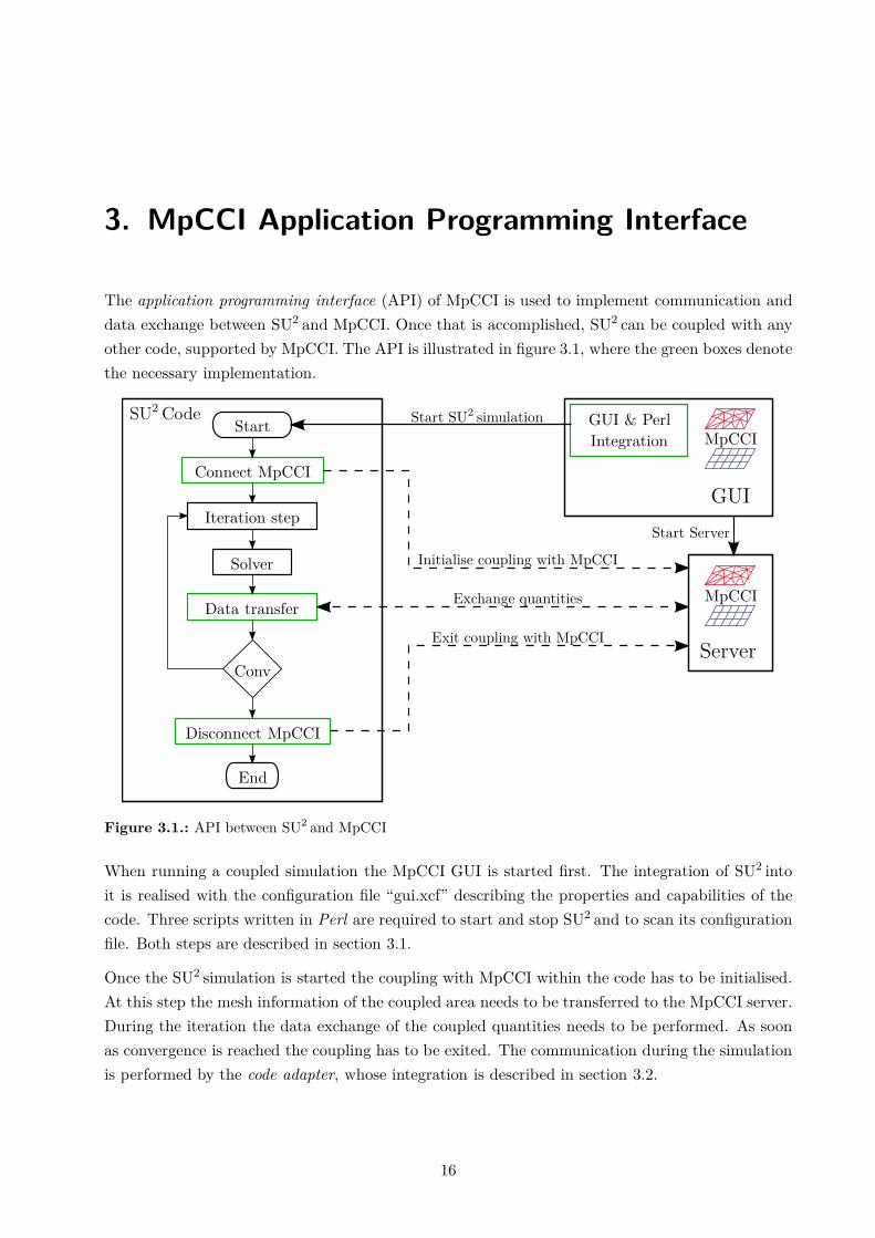
The application programming interface (API) of MpCCI is used to implement communication and
data exchange between SU2 and MpCCI. Once that is accomplished, SU2 can be coupled with any
other code, supported by MpCCI. The API is illustrated in figure 3.1, where the green boxes denote
the necessary implementation.
GUI
Server
GUI & PerlSU2 CodeStart
Connect MpCCI
Iteration step
Solver
Data transfer
Disconnect MpCCI
End
Conv
Start SU2 simulation
Start Server
Initialise coupling with MpCCI
Exchange quantities
Exit coupling with MpCCI
MpCCI
MpCCIIntegration
Figure 3.1.: API between SU2 and MpCCI
When running a coupled simulation the MpCCI GUI is started first. The integration of SU2 into
it is realised with the configuration file “gui.xcf” describing the properties and capabilities of the
code. Three scripts written in Perl are required to start and stop SU2 and to scan its configuration
file. Both steps are described in section 3.1.
Once the SU2 simulation is started the coupling with MpCCI within the code has to be initialised.
At this step the mesh information of the coupled area needs to be transferred to the MpCCI server.
During the iteration the data exchange of the coupled quantities needs to be performed. As soon
as convergence is reached the coupling has to be exited. The communication during the simulation
is performed by the code adapter, whose integration is described in section 3.2.
16
3. MpCCI Application Programming Interface
3.1. GUI and Perl Script Integration
The GUI of MpCCI is started in advance to SU2 and used to set up and start the coupled simulation.
The setup consists of five steps, which will be referred to in this section:
(1) Models
(2) Coupling
(3) Monitors
(4) Edit
(5) Go
As the GUI starts SU2 it needs to contain information about the properties of the code, which are
stored in the file “gui.xcf” located in the folder “<MpCCI_Dir>/codes/SU2” being described
in section 3.1.1. The Perl scripts, which are executed during the setup or the simulation from the
GUI are explained in section 3.1.2.
3.1.1. GUI Configuration File
The GUI configuration file consists of five important groups where the properties are stored in:
(i) Code information
(ii) Model menu entries
(iii) Component type dimensions
(iv) Supported quantities
(v) Go menu entries
(i) The very basic information of the code is stored in code info. The “unit system of” SU2 are set to
SI-units as these are the only supported units. Although SU2 supports for example the simulation
of fluid plasma as well, the “type” of the code is just set to “CFD FLUID” because it is the aim
of this work (“FluidThermal” is another possible code type). SU2 cannot be coupled with itself so
that this option is set to “false”.
Figure 3.2.: MpCCI GUI: Model step (1)
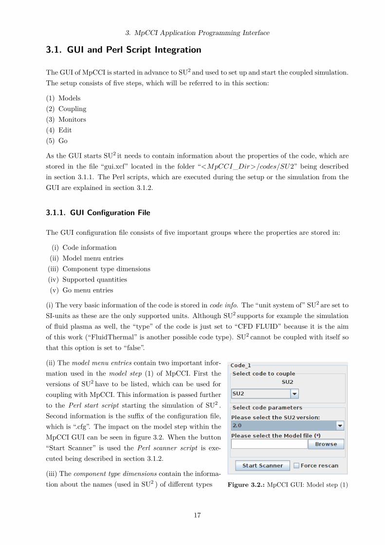
(ii) The model menu entries contain two important infor-
mation used in the model step (1) of MpCCI. First the
versions of SU2 have to be listed, which can be used for
coupling with MpCCI. This information is passed further
to the Perl start script starting the simulation of SU2 .
Second information is the suffix of the configuration file,
which is “.cfg”. The impact on the model step within the
MpCCI GUI can be seen in figure 3.2. When the button
“Start Scanner” is used the Perl scanner script is exe-
cuted being described in section 3.1.2.
(iii) The component type dimensions contain the informa-
tion about the names (used in SU2 ) of different types
17

3. MpCCI Application Programming Interface
(point, line, face, volume) for components (boundary conditions) being coupled with MpCCI. This
information is passed to the Perl scanner script. In the configuration file of SU2 no distinction is
made for the type so that the type “face” is used only for reasons of simplicity - even though for the
two dimensional case the type “line” would be appropriate. The names within the configuration
file for boundary conditions to be coupled potentially are: MARKER_EULER, MARKER_NS,
ADIABATIC_WALL, ISOTHERMAL_WALL, CATALYTIC_WALL.
(iv) The list of quantities for the coupling are defined in supported quantities. Different storage
options for the exchange of quantities may be defined before. For SU2 the standard option “direct”
is chosen. Alternatives are e.g. “user defined memory” or “buffer”.
Table 3.1.: Supported quantities of SU2 defined in “gui.xcf”
Quantity Location Send option Receive option Valid for type
Wall force Node Direct FaceRelative wall force Node Direct FaceNodal position Node Direct FaceDelta time Global Direct -
Table 3.1 shows the defined supported quantities, their saved location and the exchange option.
The aim of this work is to couple SU2 with Nastran so only the supported quantities of Nastran
will be implemented (except the velocity of the mesh’s movement - supported by Nastran). The
wall force has to be computed with the total static pressure, whereas the relative wall force is
based on the relative static pressure (e.g. in relation to the static pressure of the far field). The
quantities are defined at the nodes and are valid for faces within SU2 , which is important for the
interpolation of MpCCI and the implementation of the code adapter in section 3.2. The time step
size is an exception, because it is a global quantity and is not referred to an element type. Due to
a very complicated implementation, which would have been necessary, SU2 is only capable to send
the time step size. The impact on the coupling step (2) in the GUI of MpCCI is shown in figure
3.3a.
a) Coupling step (2) b) Go step (5)
Figure 3.3.: Setup in the GUI of MpCCI
18

3. MpCCI Application Programming Interface
(v) The go menu entries affect the go step (5) as can be seen in figure 3.3b. The initial step of
the coupling scheme may be limited to send, receive or exchange. All option are kept although
the coupling scheme used in this work does an exchange at the initial transfer being described in
section 3.2.2. Further information for the send and receive mode are given in the manual of MpCCI
Fraunhofer (2012).
The file “gui.xcf” also contains information to be passed to the Perl scripts like the configuration
file’s name of SU2 .
3.1.2. Perl Scripts
As mentioned in section 3.1.1 information are passed from the file “gui.xcf” to the Perl scripts.
Reference is made to Schwartz et al. (2005) for more information about the programming language
Perl.
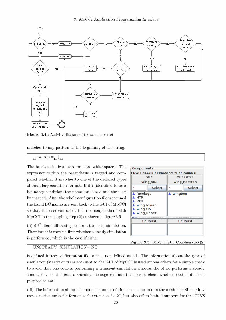
3.1.2.1. Scanner Script
The scanner script is executed in the model step (1) (figure 3.2). Its purpose is to gather the
following information from the configuration file, which is needed either for the further setup steps
or for the simulation:
(i) Names of boundary conditions being coupled potentially
(ii) Solution type: steady state or transient
(iii) Number of the model’s dimension
Furthermore information about the used coordinate system, unit system and precision of the sim-
ulation are necessary for MpCCI. As these are always the same in SU2 , they are set to Cartesian
coordinate system, SI unit system and double precision at the end of the script. The activity
diagram of the script is shown in figure 3.4.
Perl is advantageous in matching of patterns as not complicated loops are necessary. The script is
able to match a string to a regular expression, which is made up of a combination of codes (e.g.
\w+ represents one or more alphanumeric characters and \s∗ represents zero or more white spaces).
Codes and their explanation used in this script are given in table A.1 of the appendix.
(i) Each line of the configuration file is read into a string. If it matches to a comment (identified
by a leading “%”) the next line is read. As an example the regular expression matching to the
boundary condition (BC) is described. In the configuration file of SU2 a boundary condition for a
viscous wing may be defined as
MARKER_NS= ( wing_upper, wing_lower, wing_tip )
The regular expression
/ ̂ \s∗ ( \w+ ) = \s∗ \( \s∗ /
19
3. MpCCI Application Programming Interface
E�� �� ����? N� R�� ��� C� ���?A�� ��
t����
St���� ��
u��t�����
M��� ����
�n � ��
f����t�
N� N� N�
Y���� t !"��
O�!� 1 ��
��� ���?
Y��
S�#� ��
�n �Y��
S�#� f"��t ��
�n �
N�
A��t$�� ��
�n �?
��
%n&� ��'�
�� ����
Y��
S�t �t���� ��
(����n�)
*��
S�#� f"!� ����
�� ��� n�
Y��
��
*��
M���
f����t
S+²�
,-�� ���
����
Y��
L��� �#��
!"���. ��tm$
�� �������
����)
S�#� �u�/��
�� �� �������
��
Figure 3.4.: Activity diagram of the scanner script
matches to any pattern at the beginning of the string:
<word>= (
Figure 3.5.: MpCCI GUI: Coupling step (2)
The brackets indicate zero or more white spaces. The
expression within the parenthesis is tagged and com-
pared whether it matches to one of the declared types
of boundary conditions or not. If it is identified to be a
boundary condition, the names are saved and the next
line is read. After the whole configuration file is scanned
the found BC names are sent back to the GUI of MpCCI
so that the user can select them to couple them with
MpCCI in the coupling step (2) as shown in figure 3.5.
(ii) SU2 offers different types for a transient simulation.
Therefore it is checked first whether a steady simulation
is performed, which is the case if either
UNSTEADY_SIMULATION= NO
is defined in the configuration file or it is not defined at all. The information about the type of
simulation (steady or transient) sent to the GUI of MpCCI is used among others for a simple check
to avoid that one code is performing a transient simulation whereas the other performs a steady
simulation. In this case a warning message reminds the user to check whether that is done on
purpose or not.
(iii) The information about the model’s number of dimensions is stored in the mesh file. SU2 mainly
uses a native mesh file format with extension “.su2”, but also offers limited support for the CGNS
20
3. MpCCI Application Programming Interface
data format. The scanner script identifies file name and format of the mesh, which are defined in
the configuration file as:
MESH_FILENAME= and MESH_FORMAT=
The mesh file is only scanned in the case of the native format. If the cgns file format is used the
model’s number of dimensions is set to unknown, which will result in a warning message of the
GUI to avoid a model of three dimensions is coupled with a model of two dimensions.
3.1.2.2. Starter and Stopper Script
The starter script is executed when the start button in the go step (5) is pressed (figure 3.3b). It
contains the information how SU2 is executed. The name of the executable is “SU2_CFD” and its
first argument is the configuration file. The second arguments is the number of processors to be
used for a parallel simulation, which is not part of this work.
The stopper script is used whenever the user decides during a coupled simulation to perform
an regular stop so that the actual iteration is finished and the flow solution is saved. This is
accomplished by creating the file “SU2.stop” in the directory where SU2 is executed.
3.2. Code Adapter Integration
After finishing the setup (explicated in section 3.1) and starting the MpCCI server together with
the coupled codes, the server has the information about the
1. Names of the coupled parts,
2. Quantities to be exchanged,
3. Type of initial exchange for each code (send, receive or exchange),
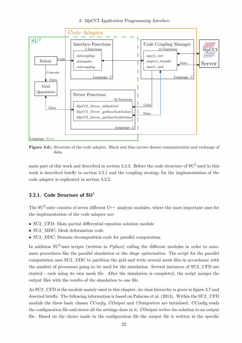
which are of major importance for the code adapter. The structure of the code adapter and its
interaction with SU2 and the MpCCI server is shown in figure 3.6.
The code adapter consists of the interface functions, the code coupling manager and the driver
functions. At run time of SU2 the interface functions have to be called. Within these the commu-
nication with the code coupling manager is established. The code coupling manger is part of the
MpCCI software package and can not be changed. It is a set of functions for the communication
between the code adapter and the MpCCI server. In order to call the functions, the header file
“mpcci.h” has to be included and the object files in “libmpcci*.a” have to be linked for the compi-
lation of the program. The functions of the code coupling manger call the driver functions, which
have to have access to the data of SU2 to gain information about the grid and the quantities of the
coupled parts. The data is then routed to the MpCCI server via the code coupling manager.
The API of MpCCI is written in C to accomplish support for the implementation of codes written
in C, C++ and Fortran. SU2 is written in C++, which has to be taken into account for the data
exchange (between code and code adapter) and the compilation of the program. The implementa-
tion of the intersection of SU2 (green box) and the code adapter (orange box) in figure 3.6 is the
21
3. MpCCI Application Programming Interface
Server
SU2
Solver
Grid
Controls
Language: C++
Calls
Data
Data
Driver Functions
MpCCI_Driver_defineGrid
MpCCI_Driver_getFaceNodeValues
MpCCI_Driver_putFaceNodeValues
32 functions
Language: C
Data
Code Adapter
Interface Functions
Language: C
initcoupling
dotransfer
exitcoupling
3 functions
Code Coupling Manager
mpcci_init
ampcci_transfer
mpcci_quit
15 functions
Language: C
Calls
Quantities
Data
MpCCI
Figure 3.6.: Structure of the code adapter. Black and blue arrows denote communication and exchange ofdata.
main part of this work and described in section 3.2.3. Before the code structure of SU2 used in this
work is described briefly in section 3.2.1 and the coupling strategy for the implementation of the
code adapter is explicated in section 3.2.2.
3.2.1. Code Structure of SU2
The SU2 suite consists of seven different C++ analysis modules, where the most important ones for
the implementation of the code adapter are:
• SU2_CFD: Main partial differential equation solution module
• SU2_MDC: Mesh deformation code
• SU2_DDC: Domain decomposition code for parallel computation
In addition SU2 uses scripts (written in Python) calling the different modules in order to auto-
mate procedures like the parallel simulation or the shape optimisation. The script for the parallel
computation uses SU2_DDC to partition the grid and write several mesh files in accordance with
the number of processors going to be used for the simulation. Several instances of SU2_CFD are
started - each using its own mesh file. After the simulation is completed, the script merges the
output files with the results of the simulation to one file.
As SU2_CFD is the module mainly used in this chapter, its class hierarchy is given in figure 3.7 and
descried briefly. The following information is based on Palacios et al. (2013). Within the SU2_CFD
module the three basic classes CConfig, COutput and CIntegration are initialised. CConfig reads
the configuration file and stores all the settings done in it. COutput writes the solution to an output
file. Based on the choice made in the configuration file the output file is written in the specific
22

3. MpCCI Application Programming Interface
Figure 3.7.: Class hierarchy in SU2_CFD, Palacios et al. (2013)
format for Tecplot or Paraview. CIntegration solves the equations describing the physical problem
(e.g. Euler equations) by calling the child classes CMultiGridIntegration or CSingleGridIntegration
depending on whether the multi-grid technique is used or not. This class initialises and connects
the classes
(i) CGeometry,
(ii) CSolution and
(iii) CNumerics
in order to integrate the equations in time and space.
a) Control volume of the dual-grid
b) Classes related to the class CGeometry
Figure 3.8.: Classes and dual-grid used by SU2_CFD for the geometry processing, Palacios et al. (2013)
(i) CGeometry reads the mesh file and contains several child classes such as CPhysicalGeometry
and CMultiGridGeometry as shown in figure 3.8b. The first generates the dual-grid using the
23

3. MpCCI Application Programming Interface
classes CPrimalGrid and CDualGrid whereas the latter constructs the coarser meshes necessary
for the multi-grid simulation. CPrimalGrid contains the different element types describing both
the volumetric grid and the boundary elements. The children CEdge, CPoint and CVertex of the
class CDualGrid are used for the dual-grid structure. CPoint represents both the grid point of the
primal mesh and the integration point used for solving the governing equations of the dual-grid.
CVertex describes a grid point of a boundary element. As can been seen in figure 3.8a the dual-grid
volume is set up by connecting the centroids, the edge-midpoints and the faces. In the case of an
two dimensional grid the edges and faces coincide.
Figure 3.9.: Fraction of the classes related to the class CSolution, Palacioset al. (2013)
(ii) In figure 3.9 a frac-
tion of the children of
the classes CSolution and
CVariable can be seen. For
a viscous problem the classes
CEulerSolution and CNSSo-
lution are initialised. The
latter class just extends the
first one with the viscous term. They call classes in CNumerics in order to discretise the equations
describing the physical problem. In addition they call CVariable and CSparseMatrix, where the
first’s subclasses contain the solution variables for each point (e.g. the conservative variables) and
the latter stores values for the Jacobians of fluxes and source terms for implicit calculations.
(iii) CNumerics contains several subclasses discretising the convective fluxes, viscous fluxes and
source terms. For an implicit solution scheme the children of CNumerics discretise the fluxes and
compute the Jacobians at each point using the subclasses of CVariable and return the results back
to CSolution, which then calls CSparseMatrix to solve the linear equation system.
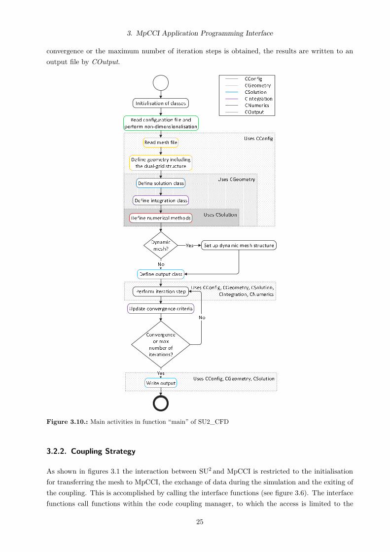
To get an impression of the interaction of the classes within SU2_CFD, the main activities of its
function “main” are described in figure 3.10, where the line colors refer to the class they belong to.
After the initialisation of the classes the configuration file is read by the class CConfig. The non-
dimensionalisation of the input values for the flow equations is performed. In addition to provided
reference values in the configuration file (e.g. for pressure, temperature, density) reference values
for e.g. time and dynamic viscosity are computed. The scheme for the computed values is given in
Palacios et al. (2013).
The mesh file is read by CGeometry and the connectivity (e.g. the neighbour points and elements
of a point) is computed as well as the dual-grid structure. CSolution then initialises different classes
referring to the solution type: Euler equations, Navier-Stokes (NS) equations, turbulence model.
The classes CIntegration and CNumerics are initialised using the information of the configuration
file concerning the definition of multi-grid technology and discretisation scheme to be used, e.g.
JST or Roe. In the case of a dynamic mesh classes for the surface and the volumetric movement
are initialised.
For the iteration step the classes CConfig, CGeometry, CSolution, CIntegration and CNumerics
are necessary. After each iteration step the convergence criteria e.g. the residual is updated. When
24
3. MpCCI Application Programming Interface
convergence or the maximum number of iteration steps is obtained, the results are written to an
output file by COutput.
U��� �������, �C�����, ��� ����
U��� �������, �C�����, ��� ����,
���������, ��������
���� �������
U��� �C�����
U��� ��� ����
����� ������ �� � �����
R��� ����������� �� � ���
p���� ���-���������� ������
R��� ���� �� �
D����� ������ ��� �����
�� ��� -��� �����
D����� �� ���� � ���
D����� �������� � ���
�� �p ������� ���� �����D������
����?
D����� ��p� � ���
P������ � ��! ��� � �"
���#�����$�
� ��o
�n�%�� ��
�������?
Up��� ���&������ �����
W�� � �n "n
Y��
��
'��
N�
(����� �n����$!) �� *�+�
�������
�C�����
��� ����
���������
��������
�.n "n
Figure 3.10.: Main activities in function “main” of SU2_CFD
3.2.2. Coupling Strategy
As shown in figures 3.1 the interaction between SU2 and MpCCI is restricted to the initialisation
for transferring the mesh to MpCCI, the exchange of data during the simulation and the exiting of
the coupling. This is accomplished by calling the interface functions (see figure 3.6). The interface
functions call functions within the code coupling manager, to which the access is limited to the
25

3. MpCCI Application Programming Interface
MpCCI development team. The functions within the code coupling manger use the driver functions
in order to gather information about the mesh and to get and set the exchanged quantities from
and onto the SU2 grid, which means that they need to have access to the data. As described in
section 3.2.1 SU2 uses classes to store information about the solution variables and the grid.
Iteration step
Language: C++
Driver Functions
MpCCI_Driver_getFaceNodeValues
MpCCI_Driver_putFaceNodeValues
Interface Functions
dotransfer
Code Coupling Manager
ampcci_transfer
Language: C
...
...
Get forces of coupled parts
Exchange with
*Forces
NASTRAN
Calls
Calls
SU2_CFD
Put displacements to coupled parts
...
...
...
...
...
...
Iteration step
Deform grid
*Displ.
SU2
Language: C Language: C
Figure 3.11.: Interaction between SU2 and MpCCI during the exchange of the quantities; The star indicatesa pointer to the quantity
The best and most efficient way of passing information of a class from one function to another is
accomplished by sending the references of the class to the other function. Given the procedure for
the exchange of quantities in figure 3.11 this leads to two major problems:
(i) The feature of classes is limited to C++ and the API is written in C.
(ii) The functions of the code coupling manager are given and can not be changed.
(i) As classes can not be handled in C, the information needed for the exchange, which is contained
in the classes (e.g. the forces), has to be extracted and saved in a struct, which can be handled
by C++ and C. The extraction is necessary for the initialisation (providing the grid data) and the
exchange of quantities. The struct and the procedure are described in detail in section 3.2.3.
(ii) The interface function dotransfer can be changed, so that passing the struct to it, which con-
tains the data is possible. Within dotransfer the code coupling manger function ampcci_transfer
has to be called, which can not be changed, so that passing additional data to it is impossi-
ble. As the driver functions need to get and set the exchanged quantities, a global struct is
useful, which is accessible within the driver functions and SU2_CFD. The concept is to save e.g.
the forces within SU2_CFD in the global struct, so that these can be used by the driver function
MpCCI_Driver_getFaceNodeValues. The computed nodal displacements of NASTRAN are saved
in a global struct within the driver function MpCCI_Driver_putFaceNodeValues so that these are
accessible within SU2_CFD to perform the mesh deformation. Three global structs are used for the
data exchange:
26

3. MpCCI Application Programming Interface
1. BOUNDARYMESH of type su2MeshBoundaries
2. SU2DATA of type su2data
3. MPCCIDATA of type mpccidata
The first one contains the information about the surface grids in SU2 needed to initialise the coupling
with MpCCI. The second and the third are used during the iteration for the quantities to be
exchanged. su2data contains the forces computed by SU2 and mpccidata the nodal displacements
computed by the partner code, which is in this work Nastran.
Another aspect to be considered for the implementation is the effort, which is necessary for others in
order to include the implemented code adapter into their version of SU2 . As the code of SU2 is open
source, users may have changed or improved the code to their needs so that a simple replacement
of the files, which are changed in this work is not the optimum. This results in the demand for
minimal changes within the function SU2_CFD and the file “SU2_CFD.cpp” so that the copy and
paste of a few lines is sufficient. On the other side the data contained in the classes of SU2 needs
to be manipulated and saved in a struct as previously mentioned, which can just be accomplished
in C++. In order to fulfill all the requirements the file “transfer.cpp” (written in C++) is created
as shown in figure 3.12, which contains the transfer functions.
Initialise MpCCI
File: SU2_CFD.cpp
Transfer Functions
dotransfer
Interface Functions
File: transfer.cpp
...
...
CConfig, CGeometry
SU2_CFD
...
SU2
File: adapter.c
Exchange data
Exit Coupling
initcoupling
exitcoupling
MpCCI_SendMesh
MpCCI_ExchangeData
MpCCI_ExitCoupling
...
Gather mesh information,write them to global struct
...
CConfig, CGeometry, CSolution
CVolumetricMovementGather pressure, compute forces
...
Perform grid deformation
...
... ...
Section 3.2.3.1
Section 3.2.3.2
Section 3.2.3.3
Figure 3.12.: Data structure for functions involved during the data exchange between SU2 and MpCCI
The transfer functions are called within SU2_CFD and used to manipulate the data given in classes
and store them into the global structs mentioned above, so that they can be used within the
interface and driver functions.
27

3. MpCCI Application Programming Interface
3.2.3. Code Adapter Implementation
The implementation of the code adapter into the SU2 code is accomplished in three steps. The
initialisation of the coupling is described in section 3.2.3.1, the exchange of quantities during the
iteration in section 3.2.3.2 and the finalisation of the coupling in section 3.2.3.3. The implementation
of each section is divided into sub steps referring to the order the functions are called (see figures
3.11 and 3.12):
(I) SU2 main function
(II) Transfer function
(III) Interface function
(IV) Driver function
Also the indexes “a” and “b” are used to indicate steps in advance to the call (a) of the next
function or after (b). (I.a) indicates the implementation within SU2_CFD prior to the call of a
transfer function, whereas (II.b) indicates the implementation within a transfer function after the
call of a interface function.
Due to the order the functions are called and the data structure (figure 3.12) - based on the coupling
strategy described in section 3.2.2 - the header files need to be included as written in algorithm
3.1.
Header file: SU2_CFD.hpp
include transfer.hpp and default header files
Header file: transfer.hpp
include config_structure.hpp, geometry_structure.hpp, solution_structure.hpp,
grid_movement_structure.hpp and adapter.h
Header file: adapter.h
include mpcci.h
Algorithm 3.1.: Header files to be included
The function SU2_CFD needs to call the transfer functions. The transfer functions have to manip-
ulate the data stored in the classes passed to it as shown in figure 3.12 so the header files of these
classes need to be included as well as “adapter.h”, which contains the declaration of the interface
functions. As the interface functions call the code coupling manager functions “mpcci.h” needs to
be included.
3.2.3.1. Coupling Initialisation
During the initialisation of the coupling the connection between the MpCCI server and SU2 is
established. Its main purpose is to provide the mesh so that MpCCI can perform the neighborhood
search and compute the transformation matrices for the exchange of quantities as shown in figure
3.13.
28

3. MpCCI Application Programming Interface
Transfer Functions Interface FunctionsSU2
initcoupling
MpCCI_SendMesh
Gather information
write them to
IV
Driver Functions
MpCCI_Driver_partUpdate
MpCCI_Driver_definePart
MpCCI_Driver_afterCloseSetup
Code CouplingManager
Calls several
mangercode coupling
ampcci_config
Define general information aboutthe grid (coordinate system,
Define the grid of coupled surfaces
Allocate memory for quantities
Allocate memory for
given by MpCCI
quantities provided
III.a
III.b
II.a
II.b
I.a
I.b
about the mesh
BOUNDARYMESH
functions
number of nodes...)
by SU2
...
...
...
...
...
...
...
Figure 3.13.: Sequence during coupling initialisation; blue: reference to the paragraphs
Before the coupling is initialised it is unknown within SU2 which surface grids of SU2 will be coupled
as this information is passed by the MpCCI GUI only to the MpCCI server. In order to provide
this information to SU2 even before the coupling, the CConfig can be modified in order to detect an
entry in the configuration file of SU2 , which contains the information of the surfaces to be coupled.
The advantage of this implementation would be the reduced number surface grids (otherwise all
surface grids have) to be saved in the global struct BOUNDARYMESH (3.2.2), which is used by
the driver functions. This leads to a reduced amount of allocated memory and computation time.
On the other side the aim of this work is to change the code of SU2 as less as possible. Also the
initialisation occurs just once per simulation and the memory used for the struct will be freed
after the initialisation so that it is more advantageous to gather the information of all surface grids
definied in the mesh file of SU2 and write them to the global struct BOUNDARYMESH.
As explicated in section 3.2.2 the transfer function is used to manipulate the information about the
grid and store it into the global struct of type su2MeshBoundaries (listing 3.1), which is initialised
in the header file “adapter.h”. Its information are used by the driver functions partUpdate and
definePart, which calls are shown in figure 3.13. The struct has to contain the information of
all surface grids potentially being coupled. Therefore up to three instances of pointers are used to
create data fields, where the first instance is used for the different surfaces. The second and third
instance can be interpreted as a vector or a matrix respectively. Below the vector and matrix are
used in this context. Vectors are used to store the node numbers composing a surface grid and the
name of each surface grid (the name has to be stored using the data type char as the C language
does not support string). Matrices are used to store the coordinates of each node and the node
numbers each element is composed of. The position in the matrix (the “row”) of the coordinates is
29

3. MpCCI Application Programming Interface
Listing 3.1: Global struct BOUNDARYMESH of type su2MeshBoundaries used for grid data
// adapter . hstruct su2MeshBoundaries {
unsigned short nCouple ;char∗∗ coupleName ;bool threeDim ;unsigned long∗ nPointSurface , nElemSurface ;unsigned long∗∗ coupleNodeNumber ;double ∗∗∗ coupleNodeCoord ;unsigned long ∗∗∗ coupleElemNodes ;unsigned short∗ maxNodeElemType ;
} ;extern su2MeshBoundaries BOUNDARYMESH;
// adapter . csu2MeshBoundaries BOUNDARYMESH;
related to the position in the vector of the variable coupleNodeNumber so that for one position the
corresponding node number and its coordinates can be extracted easily. The struct also contains
some basic information about the dimension of the physical problem and the number of nodes and
elements of each surface grid. The variable maxNodeElemType contains for each surface grid the
used element type, which has most nodes. As this struct has to be of type global it is defined in
the header file and in the c file with the name BOUNDARYMESH. The extern in the header file is
necessary due to the usage of the struct in the external files “transfer.cpp” and “SU2_CFD.cpp”
written in C++. Referring to figure 3.13 the implementation is explicated below.
(I.a) As the information about the grid needs
to be available before the coupling is initialised,
the transfer function MpCCI_SendMesh is called
before the first iteration step of SU2 is per-
formed.
(II.a) The implementation of MpCCI_SendMesh
up to the call of the interface function
initcoupling is shown in algorithm 3.2. Its
purpose is the gathering of the information of
the grid and its storage to the variables of the
struct BOUNDARYMESH. The class CConfig contains the number of surface grids and their names,
which are read from the SU2 configuration file (figure 3.10). The number of grids is necessary among
others for the dynamic allocation of memory. Whenever memory is allocated dynamically, it is made
sure that the heap can provide it or the program is aborted. The names of the grids are necessary
to identify the coupled grids within the interface functions as the SU2 does not use ids for the
grids. The class CGeometry contains the remaining information about the grids. Within SU2 the
boundary conditions are always saved in the same order, which means that e.g. the first name of a
30

3. MpCCI Application Programming Interface
boundary condition matches to the first set of node numbers. The same order is used to write the
data to BOUNDARYMESH.
int MpCCI_SendMesh(CConfig, CGeometry){
/* all the data in this function is written to the variables of
BOUNDARYMESH of type struct su2MeshBoundaries */
get number of dimensions and boundaries −→ threeDim, nCouple;
allocate memory for first instance in BOUNDARYMESH;
for (all surface grids in CConfig){
get name of grid −→ coupleName;
get number of nodes and elements −→ nPointSurface, nElemSurface;
allocate memory for second instance in BOUNDARYMESH;
for (all nodes of each surface grid){
get global node number −→ coupleNodeNumber;
allocate memory for third instance in BOUNDARYMESH;
get coordinates of node −→ coupleNodeCoord;
for (all elements of each surface grid){
allocate memory for third instance in BOUNDARYMESH;
get element type −→ first entry of coupleElemNodes;
set maxNodeElemType to type with least nodes;
for (all nodes of each element){
get node numbers of element −→ coupleElemNodes;
if (element contains more nodes than maxNodeElemType){
set maxNodeElemType to new element type;
get type of simulation, iteration step, current unsteady time step and physical time;
call function initcoupling and pass information of last line;
/* ... continuation in II.b */
Algorithm 3.2.: Implementation of MpCCI_SendMesh before call of initcoupling
CGeometry provides methods to get the number of elements and nodes for a “marker” (marker
is the keyword within the SU2 code for boundary condition). This information is used to allocate
the correct amount of memory for the node numbers, coordinated and elements definition for each
surface grid. CGeometry contains a vector of type CVertex for each marker. This vector contains
dual grid information for each node of the marker e.g. the global node number, relative coordinates
of node (relative to the cell of the dual grid) and normal vector. A method is provided to get the
global node number, which then can be used to get the global coordinates of the node. The class
CVertex is only used for nodes of markers (boundary conditions), whereas a vector of type CPoint
is used in CGeometry to store information about the nodes of the entire CFD grid. The position in
this vector is related to its global node number. CPoint provides a method to get the coordinates
of the node.
The elements of a marker are stored within CGeometry in the matrix of type CPrimalGrid. The
first instance is used for the markers and the second for the elements each marker contains. A
31
3. MpCCI Application Programming Interface
method of CPrimalGrid is used to get the number of nodes the element is composed of to allocate
memory for the corresponding variable of the struct. For each element memory for one additional
entry is allocated, which is used to store the information of the element type in the first entry using
the VTK nomenclature (Kitware 2010) given in table 3.2. The following entries (beginning with
the second) are used for the global node numbers the element is composed of.
Table 3.2.: VTK nomenclature of two dimensional element types used in SU2
Identifier 3 5 9
Element type Line Triangle Rectangle
Number of nodes 2 3 4
The domain the surface grid describes can bet approximated with different types of elements
e.g. a composition of triangles and rectangles. MpCCI needs the information about the element
type containing the most nodes, which is used in the surface grid. As the identification number is
increasing with more nodes used to describe an element (table 3.2), the new identification is written
to the variable maxNodeElemType of the struct BOUNDARYMESH, if it is greater than the one
of the last element. After the loop over all surface grids is finished the struct BOUNDARYMESH
contains all information needed by the driver functions later on.
For the initialisation of the coupling information about the current iteration number, current un-
steady time and time step size is necessary. Also the type of simulation (steady or transient) is im-
portant although most of the aeroelastic cases will deal with unsteady simulations. These informa-
tion are gathered using methods of CConfig and passed to the interface function initcoupling.
(III.a) As shown in figure 3.13 initcoupling
calls several functions of the code coupling man-
ager to initialise the communication between
the MpCCI server and SU2 , for which MpCCI
uses several structs. Four of them (listing A.2
in the appendix) are important for the initialisation and their variables used in this work are de-
scribed briefly. The structs are declared in “mpcci_types.h” and their detailed description is given
in Fraunhofer (2012).
The transfer information are defined in the struct MPCCI_TINFO. It contains more than 40 vari-
ables so that just the most important ones for this work are explained. The state states the status
of the coupling:
-1 : Disconnected from the server
0 : Nothing done before
1 : Initially connected to the server
>1 : Initialisation done and at least one data transferIf MpCCI is used mpcci_used is true. The remaining important variables are the current iteration
number, the current physical time and the current time step size, which need to be updated before
amppci_transfer is called.
The struct MPCCI_CINFO contains some code specific information like the name of the code, the
initial iteration number and physical time. Also the number of server clients and the number of
32

3. MpCCI Application Programming Interface
processors for parallel computing of SU2 are part of it.
The struct MPCCI_JOB contains a chain of structs of type MPCCI_SERVER in the case multiple
servers are used.
MPCCI_DRIVER contains all the driver functions. The complete definition can be found in Fraun-
hofer (2012).
All the structs except MPCCI_CINFO are defined as global variables within the file “adapter.c”
and therefore available withing the interface and driver functions. Algorithm 3.3 shows the imple-
mentation of initcoupling before the call of ampcci_config. Its calling sequence depends on the
specifications of MpCCI given in Fraunhofer (2012).
int initcoupling(ExtIter, Current_UnstTime, Delta_UnstTime, UnsteadySimulation){
if (MpCCI already initialised){
return 0;
define output functions −→ call umpcci_msg_functs;
define a message prefix −→ call umpcci_msg_prefix;
call ampcci_tinfo_init(&MPCCI_TINFO);
if (transfer information is not set up successful){
MPCCI_TINFO.state = -1;
return -1;
set current iteration number, time and time step size −→ MPCCI_TINFO;
set variables of MPCCI_CINFO ; /* 1 client, 1 processor */
get MPCCI_JOB −→ call mpcci_init(MPCCI_CINFO) to establish a connection to the
server;
call ampcci_config(MPCCI_JOB, &MPCCI_DRIVER);
/* ... continuation in III.b */
Algorithm 3.3.: Implementation of initcoupling before call of ampcci_config
In the case MpCCI has been already initialised initcoupling is finished, which can not happen
in the procedure used as the initialisation is done before the iteration loop in SU2 is performed.
Before any other code coupling manger functions are called the message functions for the output
of MpCCI have to be defined by calling umpcci_msg_functs. Two different message functions are
defined in “adapter.c”. The function adapter_output is used for normal messages and warnings,
whereas the function error is used for error messages. In order to identify easily the output of
MpCCI umpcci_msg_prefix is called and passed the message prefix “MpCCI: “.
The reference of mpcciTinfo is passed to ampcci_tinfo_init, which determines the transfer infor-
mation selected in the MpCCI GUI “go step” (figure 3.3b) and stores them in the passed struct.
If the transfer information was not set up successfully the MpCCI state is set to “disconnected
from the server” and initcoupling is finished returning -1. In the case of a successful setup,
the struct MPCCI_CINFO is initialised with initial values for physical time and iteration number
of the simulation. Both are in the current version of SU2 initially always zero. In the case of a
restart of a simulation, SU2 sets both values again to zero. However the current physical time,
time step size and iteration number are gathered in MpCCI_SendMesh (algorithm 3.2) and passed
to initcoupling in the case this is changed in future versions of SU2 . Referring to table 3.3 the
33

3. MpCCI Application Programming Interface
type of coupling can be influenced. For an unsteady simulation, which will cover most cases, the
code can be designed to be explicit or implicit. For an explicit code the iteration number has to be
set to -1, whereas the real iteration number is set for an implicit code, Fraunhofer (2012). Using
the implicit formulation enable the code to request data during the same physical time step. The
number of clients and processors are both set to one as this version of the code adapter is not yet
implemented for parallel computation. MPCCI_CINFO is passed to mpcci_init which establishes
a connection to the server and returns a pointer to the struct MPCCI_JOB.
Table 3.3.: Coupling type depending on values set in the structs MPCCI_CINFO and MPCCI_TINFO
Coupling scheme Iteration number Current unsteady time Current time step size
Steady Real value -1 -1
Transient explicit -1 Real value Real value
Transient implicit Real value Real value Real value
The structs MPCCI_JOB and MPCCI_DRIVER are passed to ampcci_config. MPCCI_JOB
contains the connection information to the MpCCI server and MPCCI_DRIVER the driver func-
tions. As already mentioned there are 32 driver functions, of which six are needed in this work. To
tell the code coupling manager, which driver functions will be used, the one, which are not used, are
defined with “NULL” in the global struct MpCCIDriverFunctions declared in “adapter.c” (listing
A.2). In addition to this information ampcci_config gets the information about the components
(surface grids) to be coupled and the quantities to be exchanged (selected in the MpCCI GUI
figures 3.3a and 3.5). After a loop over all the coupled components is performed and the driver
functions are called in the following order:
1. MpCCI_Driver_partUpdate
2. MpCCI_Driver_definePart
3. MpCCI_Driver_afterCloseSetup
(IV) In addition to the structs mentioned above MPCCI_PART and MPCCI_QUANT are used
by the driver functions during the initialisation and the data exchange (section 3.2.3.2), which
are shown in listing A.1 of the appendix. MpCCI provides macro functions (interpreted by the
preprocessor) in order to access the variables of these structs (using the “#define” command).
The function MpCCI_Driver_partUpdate is
called by the code coupling manager for each
surface grid to be coupled (called “parts” in
MpCCI as their basic information are stored in
MPCCI_PART). For a wing, which consists of
three surface grids (tip, upper and lower side) the function is called three times for SU2 . It is used
to update the components. As shown in algorithm 3.4 a loop over all surface grids in BOUND-
ARYMESH is used to get the index of the surface grid, which name matches to the name of
MPCCI_PART passed to the function. The index is saved to the part as well as the number of
points and elements it contains. Also the number of dimensions of the physical problem and the
used coordinate system (always Cartesian for SU2 ) are set.
34

3. MpCCI Application Programming Interface
int MpCCI_Driver_partUpdate(MPCCI_PART, MPCCI_QUANT){for (all surface grids in BOUNDARYMESH ){
find matching grid in BOUNDARYMESH −→ MPCCI_PART.partID;
get number of points −→ MPCCI_PART.nnodes;get number of elements −→ MPCCI_PART.nelems;if (three dimensional case){
set coordinate system to 3d Cartesian −→ MPCCI_PART.csys;
else{set coordinate system to 2d Cartesian −→ MPCCI_PART.csys;
return 0;
Algorithm 3.4.: Implementation of MpCCI_Driver_partUpdate
To define a mesh two different procedures are provided by MpCCI, Fraunhofer (2012):
1. Definition of MpCCI_Driver_definePart: The code is responsible for the management of
memory.
2. Definition of MpCCI_Driver_partInfo, MpCCI_Driver_getNodes and MpCCI_Driver_getElems:
The coupling manger is responsible for the management of memory.
To have a greater influence the first option is
chosen. As shown in algorithm 3.5 three cou-
pling manager functions need to be called: defp
(define part), pnod (define part nodes) and pels
(define part elements). In addition to values
specific for the function, all of them need the partID and the MPCCI_SERVER the part is asso-
ciated with. The partID of MPCCI_PART is used to obtain the values from BOUNDARYMESH
for the corresponding surface grid and collect them in a vector. The vector of node numbers and
coordinates the part consists of is passed to smppci_pnod in addition to the used coordinate system,
which was already defined in MpCCI_Driver_partUpdate. A distinction is done for the number
of dimensions of the physical problem. It has to be taken into account for the generation of the
structural grid that SU2 defines coordinates of two dimensions in the x-y plane.
Depending on the element type (obtained from BOUNDARYMESH using VTK nomenclature of
table 3.2) the element is defined by its node numbers and the type, which are saved in the corre-
sponding vectors. MpCCI supports many different types of elements, whereof only the linear types
for line, triangle and quadrilateral elements are used by SU2 . The vectors for the element types
and node numbers are passed to smppci_pels and the definition for the part is completed.
Before returning to initcoupling according to
figure 3.13, MpCCI_Driver_afterCloseSetup
(called by the coupling manager) is used among
others for the management of memory. After
the parts are defined it is known (within the
code adapter) which surface grids are coupled. This information is saved in the global struct to
transfer this information to the transfer functions. The initialisation for the struct MPCCIDATA
is done in the header file “adapter.h” (listing 3.2).
35

3. MpCCI Application Programming Interface
int MpCCI_Driver_definePart(MPCCI_SERVER, MPCCI_PART){get partID of MPCCI_PART;call smpcci_defp(*server, partID, csys, nNodes, nElems, name);if (smpcci_defp successful){
allocate memory for *nodenumbers and *coordinates;for (all nodes of MPCCI_PART ){
get node numbers and coordinates −→ *coordinates, *nodenumbers;
call smpcci_pnod(*server, partID, csys, nNodes, *coordinates, *nodenumbers, ...);free memory;
if (smpcci_defp and smpcci_pnod successful){allocate memory for element nodes and types of elements;for (all elements of MPCCI_PART ){
switch (element type){get nodes of element −→ *elemNodes;get element type −→ *elemTypes;
call smpcci_pels(*server, partID, nElems, *elemTypes, *elemNodes, ...);free memory;
if (all function calls were successful){return 0;
else{return -1;
Algorithm 3.5.: Implementation of MpCCI_Driver_definePart
Listing 3.2: Global struct for data received from MpCCI and/or gathered within the interface functions
// adapter . h
struct mpccidata {
bool coup ledS imulat ion ;
unsigned short nSur face ;
bool threeDim ;
unsigned short ∗ sur faceID ;
char ∗∗ surfaceName ;
double ∗∗∗ coup ledSur faceValues ;
bool ∗ remesh ;
double Delta_UnstTime ;
} ;
extern mpccidata MPCCIDATA;
// adapter . c
mpccidata MPCCIDATA;
The implementation of MpCCI_Driver_afterCloseSetup is shown in algorithm 3.6. Its purpose
is to save some basic information about the coupled parts in the global struct MPCCIDATA and
allocate memory for its variables. MpCCI provides some loop functions over objects of a struct
interpreted by the preprocessor. The loops make use of a variable in a struct, which points to the
36

3. MpCCI Application Programming Interface
next struct of the same type (e.g. the struct “part1” contains a variable pointing to the struct
“part2” - both of same type). This pointer always has the name next in all structs it is provided.
MpCCI_Driver_afterCloseSetup does not get any variables so that the global struct MPCCI_JOB
(listing A.2) is used to loop over its servers it is connected with (in the case of serial computation
there is just one server). For each MPCCI_SERVER a loop over its parts is performed to count
the number of coupled surface grids. This number is stored in MPCCIDATA and used to allocate
memory for the first instance of pointers in MPCCIDATA. The same loops are performed again to
store the surfaces’ name and ID to MPCCIDATA. Also the remesh flag for each surface grid is set
to false (more information is given in section 3.2.3.2). Memory is allocated for the second instance
depending on the number nodes. The third instance needs memory for three values to store the
nodal displacements in a vector.
void MpCCI_Driver_afterCloseSetup(void){
get number of dimensions −→ MPCCIDATA.threeDim;
for (each server in MPCCI_JOB){
get parts of MPCCI_SERVER;
for (each part of MPCCI_SERVER){
nSurface++;
set number of coupled surfaces −→ MPCCIDATA.nSurface;
allocate memory for first instance of MPCCIDATA;
for (each server in MPCCI_JOB){
get parts of MPCCI_SERVER;
for (each part of MPCCI_SERVER){
get part’s name −→ MPCCIDATA.surfaceName;
get partID −→ MPCCIDATA.surfaceID;
set MPCCIDATA.remesh to false;
allocate memory for second instance of MPCCIDATA;
for (each node in MPCCIDATA){
allocate memory for third instance of MPCCIDATA;
Algorithm 3.6.: Implementation of MpCCI_Driver_afterCloseSetup
(III.b) After the code coupling manager func-
tion ampcci_transfer has finished the calls of
the driver functions, the control is given back to
the interface function initcoupling as shown
in figure 3.13. The implementation after the
call is shown in algorithm 3.7.
If mpcci_init created an MPCCI_JOB, but ampcci_config was not successful the coupling is
quit and -1 is returned to the transfer function MpCCI_SendMesh to state the failure of initialising
the coupling. This happens for example if MpCCI is not able to match the surface grids. In the
case an MPCCI_JOB could not be created, which should occur only for a bad implementation of
37

3. MpCCI Application Programming Interface
int initcoupling(ExtIter, Current_UnstTime, Delta_UnstTime, UnsteadySimulation){/* continuation after call of ampcci_config */
if ((MPCCI_JOB created) and (ampcci_config not successful)){call mpcci_quit to abort the coupling;return -1;
if (MPCCI_JOB was not created){MPCCI_TINFO.state = -1;return -1;
else{MPCCI_TINFO.state = 1;MPCCI_TINFO.used = 1;return 0;
Algorithm 3.7.: Implementation of initcoupling after call of ampcci_config in algorithm 3.3
the code adapter, the state of MPCCI_TINFO is set to “disconnected from the server” and -1 is
returned. Otherwise the initialisation was successful the state and use of MPCCI_TINFO are set
to 1 and succeed is returned to MpCCI_SendMesh.
(II.b) After the interface function initcoupling
is finished, the control is given back to
MpCCI_SendMesh as shown in figure 3.13.
If the coupling was initialised successfully
initcoupling returns 0 and the flag for a cou-
pled simulation is set to true and vice versa as shown in algorithm 3.8. The variable for a cou-
pled simulation is located in the global struct SU2DATA (listing 3.3) initialised in the header file
“adapter.h”. It is used to store data computed by SU2 .
Listing 3.3: Global struct for data computed by SU2 within the transfer functions
// adapter . h
struct su2data {
double ∗∗∗ coup ledSur faceValues ;
double Delta_UnstTime ;
bool volumeRemeshed ;
} ;
extern su2data SU2DATA;
// adapter . c
su2data SU2DATA;
As can be seen in algorithm 3.8 the allocated memory for the pointers in BOUNDARYMESH is
freed. In addition to allocate memory for the pointer in SU2DATA, the flag for a coupled simulation
is used to skip the data exchange (section 3.2.3.2) in the case SU2 is used without being coupled with
MpCCI. The coupled surface grids are identified in SU2 by matching the name in MPCCIDATA
to the available surface grids in CConfig. The number of coupled surface grids and their number
38
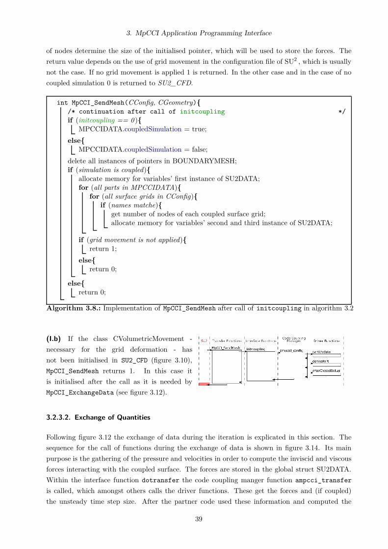
3. MpCCI Application Programming Interface
of nodes determine the size of the initialised pointer, which will be used to store the forces. The
return value depends on the use of grid movement in the configuration file of SU2 , which is usually
not the case. If no grid movement is applied 1 is returned. In the other case and in the case of no
coupled simulation 0 is returned to SU2_CFD.
int MpCCI_SendMesh(CConfig, CGeometry){/* continuation after call of initcoupling */
if (initcoupling == 0 ){MPCCIDATA.coupledSimulation = true;
else{MPCCIDATA.coupledSimulation = false;
delete all instances of pointers in BOUNDARYMESH;if (simulation is coupled){
allocate memory for variables’ first instance of SU2DATA;for (all parts in MPCCIDATA){
for (all surface grids in CConfig){if (names matche){
get number of nodes of each coupled surface grid;allocate memory for variables’ second and third instance of SU2DATA;
if (grid movement is not applied){return 1;
else{return 0;
else{return 0;
Algorithm 3.8.: Implementation of MpCCI_SendMesh after call of initcoupling in algorithm 3.2
(I.b) If the class CVolumetricMovement -
necessary for the grid deformation - has
not been initialised in SU2_CFD (figure 3.10),
MpCCI_SendMesh returns 1. In this case it
is initialised after the call as it is needed by
MpCCI_ExchangeData (see figure 3.12).
3.2.3.2. Exchange of Quantities
Following figure 3.12 the exchange of data during the iteration is explicated in this section. The
sequence for the call of functions during the exchange of data is shown in figure 3.14. Its main
purpose is the gathering of the pressure and velocities in order to compute the inviscid and viscous
forces interacting with the coupled surface. The forces are stored in the global struct SU2DATA.
Within the interface function dotransfer the code coupling manger function ampcci_transfer
is called, which amongst others calls the driver functions. These get the forces and (if coupled)
the unsteady time step size. After the partner code used these information and computed the
39

3. MpCCI Application Programming Interface
nodal displacements, these are saved by the driver function in the global struct MPCCIDATA.
The transfer function MpCCI_ExchangeData moves the coupled surface in accordance with the
computed displacements to the new position. Based on the type of mesh deformation specified
in the configuration file of SU2 the deformation of the volumetric grid is performed and the next
iteration step is done.
Transfer Functions Interface FunctionsSU2
dotransfer
MpCCI_ExchangeData
Gather pressure
inviscid forces
IV
Driver Functions
MpCCI_Driver_getFaceNodeValues
MpCCI_Driver_getGlobValues
MpCCI_Driver_putFaceNodeValues
Code CouplingManager
Update time
informationand iteration
ampcci_transfer
get forces
get time step size
put nodal displacements
Perform grid
III.a
III.b
II.a
II.b
I.a
I.b
compute viscous and
write them to
...
...
...
...
...
...
...
SU2DATA
deformation
Figure 3.14.: Sequence during exchange of data; blue: reference to the paragraphs
The implementation is described below (following the same procedure as in section 3.2.3.1) in
paragraphs referring to figure 3.14.
(I.a) In the case of an successful initialisation
the flag for a coupled simulation is set to true
within MpCCI_SendMesh (algorithm 3.8). If the
simulation is a coupled simulation, the transfer
function MPCCI_ExchangeData is called within
SU2_CFD after each iteration step.
(II.a) As Nastran can be coupled only receiv-
ing forces they need to be computed in advance
using the pressure, which is done in the transfer
function MpCCI_ExchangeData. Its implemen-
tation is shown in algorithm 3.9. Performing a
loop over the coupled surface grids stored in the struct MPCCIDATA the matching surface grids
40

3. MpCCI Application Programming Interface
defined in CConfig are found by comparing their names. During a loop over the vertices of each
coupled grid the
(i) inviscid force due to the static pressure and the
(ii) viscous force due to friction
are computed for each node and stored in the struct SU2DATA.
bool MpCCI_ExchangeData(CConfig, CGeometry, CSolution, CVolumetricMovement){for (each surface grid in MPCCIDATA){
for (each grid in CConfig){if (grids match){
for (each point of coupled surface grid){get pressure and normal vector;compute area of surface element of dual grid;compute inviscid force;if (viscous flow){
get viscosity and velocities;compute viscous force;
compute sum of forces −→ SU2DATA.coupleName;
get unsteady time step size −→ SU2DATA.Delta_UnstTime;get type of simulation, iteration step, current unsteady time step and physical time;call function dotransfer and pass information of last line;/* ... continuation in II.b */
Algorithm 3.9.: Implementation of MpCCI_ExchangeData before the call of dotransfer
(i) CSolution contains the class CVariable for each node. The global node number has to be
used to use the methods of CVariable. In the actual version of SU2 the pressure has to be gathered
differently for compressible and incompressible simulations. For a compressible simulation a method
of CVariable can be used to get the pressure directly. In the incompressible case a method has to
be used to get the solution vector, where the first entry is the pressure. It was explicated in section
3.2.1 that the solution variables are non-dimensionalised in SU2 after the classes are initialised
(figure 3.10). For computing the force it is therefore necessary to multiply the gathered pressure
with the reference pressure stored in CConfig.
During the definition of the dual-grid structure in SU2 (figure 3.10) the normal vector for the surface
grids are computed. Figure 3.15a shows the compuation of the normal vector of a quadrilateral
surface grid. Having the edge based dual grid structure and the center of gravity for each element,
the vectors ~v, ~u1 and ~u2 are computed. Using the cross product of them results in the normal
vectors ~n11 and ~n12. The magnitude of the resulting normal vector is twice the amount of the area
of the triangle, which is composed of ~u1, ~v and the connecting edge. Therefore the magnitude of
~n1 = 1/2 ( ~n11 + ~n12) is equal to the area of the part of the primal grid element, which also belongs
to the dual-grid element. The normal vector of the dual grid element is computed in SU2 by adding
the two normal vectors of each surrounding primal grid element.
Adding the vectors of the primal grid results in an error of magnitude, which is shown in figure
3.15b. The magnitude of the normal vector of the dual grid is smaller than the area of the dual
41

3. MpCCI Application Programming Interface
Primal grid
Dual grid
~v
~u1
~u2~n11
~n22
~n
x
yz
~n2
a) Computation of the normal vector of the dual-grid
x
z
~n1
~n2
~n
b) Error of magnitude of the normal vec-tor of the dual-grid
Figure 3.15.: Normal vector computation of surface grids in SU2
grid element it relates to. This error increase with the angle between the surface elements. This
problem can be solved by normalising the normal vector in accordance to the sum of the magnitudes
of the normal vectors of the primal grid, which compose the normal vector of the dual grid. This
would make changes within the SU2 routines necessary. On the other side this error becomes only
significant for bigger angles with a big element size, which is rare in CFD grids, as usually the
element size decreases with great changes of the surface. For this reason the error is accepted, but
should be taken into account for the interpretation of simulation results.
The normal vector is stored within SU2 in CVertex and a method is provided to get it. Computing
its magnitude and multiplying it with the pressure results in the magnitude of the inviscid force
for each node. The vector of the force is computed by multiplying the magnitude of the force with
the normal vector and inverting it as the normal vector is pointing outwards from the surface, but
the force due to the pressure has to point onto the surface.
When computing the inviscid force for an incompressible flow, it has to be taken into account that
the static pressure is computed as a difference (relative pressure or gauge pressure) to the ambient
pressure (inflow or far field condition) for an incompressible simulation. In this case the ambient
pressure is set to zero during the initialisation, as the solution is independent of it. Therefore the
static pressure on the surface can be negative due to friction losses and accelerated flow conditions.
The negative pressure results in a force pulling on the surface.
Flow
p∞, M∞ < 0.3
p∞ > pl > pu
pl > 0
pu < 0 pu > 0
pl > 0
Incompressible (p∞ = 0) Compressible (p∞ > 0)
Figure 3.16.: Equivalence of applying the forces on a thin plate
Figure 3.16 shows the equivalence of applying the forces on a thin plate. The Mach number of
the flow is smaller than 0.3 so that the flow is treated as an incompressible flow. For these inflow
conditions the impact on the forces using an incompressible and compressible formulation is shown.
42

3. MpCCI Application Programming Interface
As the inflow pressure is set to zero in the case of an incompressible formulation the pressure on
the upper side is negative and the resulting force is pulling on the upper surface. Using the
compressible formulation results in a positive pressure on both sides, whereas the pressure on the
lower side is greater compared with the incompressible formulation. In both cases the difference
between the upper and lower side is the same so that the net force is the same for a surface,
which is wetted with the flow on all sides. The resulting deformation is therefore also the same
assuming the (de)compression of the plate itself due to the pressure is negligible in comparison to
the deformation (e.g. bending) due to pressure difference between upper and lower side.
In the case of a compressible simulation a reference pressure for the non-dimensionalisation can be
defined within the configuration file of SU2 (default: pref = 1 N/mm). For the incompressible case
SU2 overwrites this value by the computed reference pressure pref = ρref ∗ v2ref. This results in the
problem that an absolute pressure can not be computed for an incompressible case as the reference
pressure can not be defined by the user. Adding an additional entry to the configuration file would
result in necessary changes in CConfig, which is not desirable for reasons of easy implementation
of the code adapter by other users. In addition the only problematic situations with coupling an
incompressible flow occur for:
1. coupled surface is only wetted with the flow on one side and
2. the structure of the coupled surface is wetted on all sides, but has a very small Young’s
module resulting in a compression of the structure being not anymore negligible.
(ii) In order to compute the force due to friction the element area and the wall shear stress are
necessary. In (i) the computaion of the element area was already explicated. The wall shear
stress is not stored in any class as a variable so it needs to be computed. Therefore the viscosity
and the velocity for each node have to be gathered. The viscosity is store within CSolution in
CVariable, defined for each node. Depending on the type of flow (compressible or incompressible)
the corresponding method is used to get the viscosity. As is non-dimensionalised this viscosity
needs to be multiplied with the reference viscosity stored in CConfig. The force due to friction is
computed
~F = τ · ~n A , (3.1)
where A is the area, ~n the normal vector of the surface element and τ the viscous shear stress
tensor, which elements are referring to Hirsch (2007) defined as
τij = µ
[(∂vj
∂xi+
∂vi
∂xj
)−
2
3
(~∇ · ~v
)δij
]. (3.2)
This relation is only valid for a Newtonian fluid. The gradients are stored in CVariable and are
gained by using the provided method. The viscous force is computed using equations 3.1 and 3.2 in
the case of an viscous flow. The sum of inviscid and viscous force is stored in the struct SU2DATA.
The interface function dotransfer is called providing the current iteration step, unsteady time
step size, physical time and the type of simulation (steady or transient).
43

3. MpCCI Application Programming Interface
(III.a) The implementation of dotransfer
is shown in algorithm 3.10. After its call
initcoupling is called in the case MpCCI has
not been initialised, which should not occur. In
the case MpCCI was initialised, but it is not
used (due to a failure during the initialisation e.g. the neighborhood search), dotransfer returns
−1 to state that the exchange of data failed. Depending on the simulation type the time step size,
current time and iteration step are set in accordance to table 3.3. After ampcci_transfer is called
passing the mpcciJob created in initcoupling and mpcciTinfo, with the information about time
and iteration.
int dotransfer(ExtIter, Current_UnstTime, Delta_UnstTime, UnsteadySimulation){if (MpCCI is not initialised){
call initcoupling;
if (MpCCI is not used){return -1;
if (transient simulation){mpcciTinfo.iter = -1;mpcciTinfo.time = Current_UnstTime;mpcciTinfo.dt = Delta_UnstTime;
else{mpcciTinfo.iter = ExtIter;mpcciTinfo.time = -1;mpcciTinfo.dt = -1;
call ampcci_transfer(mpcciJob, &mpcciTinfo);/* ... continuation in III.b */
Algorithm 3.10.: Implementation of dotransfer before the call of ampcci_transfer
The code coupling manger function ampcci_transfer checks if any partner code is waiting for
quantities taking the initial transfer action for the code (send, receive, exchange) into account.
After it checks the availability of quantities of each partner code. After its calling the driver
functions of the partner codes for sending and receiving based on the coupling scheme. After it
returns to the calling code. For the current implementation SU2 is supposed to be the partner
code first performing the iteration step (figure 2.9). Therefore ampcci_transfer calls the driver
functions in the following order as shown in figure 3.14:
1. MpCCI_Driver_getFaceNodeValues
2. MpCCI_Driver_getGlobValues
3. MpCCI_Driver_putFaceNodeValues
(IV) The defined driver function specify how
MpCCI needs to treat the coupled quantities.
SU2 stores the values at the nodes and they are
valid on faces. For a two dimensional grid it
44

3. MpCCI Application Programming Interface
would be more precise to couple a line, but for
reasons of less effort in implementation they are treated as faces as well.
As shown in algorithm 3.11 getFaceNodeValue gets the structs MPCCI_PART and MPCCI_PART
(listing A.1) and the pointer to the values of the coupled quantities. The surface ID stored in
MPCCI_PART is used to identify the related surface in SU2 using the struct MPCCIDATA. De-
pending on the coupled quantity’s type (wall force or relative wall force) the values are stored in
the pointer to the values. This function is called several times if the coupled surface consists of
more than one part.
int MpCCI_Driver_getFaceNodeValues(MPCCI_PART, MPCCI_QUANT, *values){get surface ID of MPCCI_PART;get matching surface stored in MPCCIDATA.surfaceID;get number of nodes from MPCCI_PART;switch (quantity type){
for (all nodes of surface){get quantity from SU2DATA −→ *values;
Algorithm 3.11.: Implementation of MpCCI_Driver_getFaceNodeValues
The driver function getGlobValues is only
called if a coupling of the time step size was cho-
sen in the MpCCI GUI. The procedure is very
similar to algorithm 3.11. The time step size,
which is constant in SU2 for the current version
is taken from SU2DATA and stored in the pointer to the values passed to the driver function.
The implementation of putFaceNodeValues is
very similar to getFaceNodeValues with one
important difference shown in algorithm 3.12.
After the quantities (nodal displacements) are
store in the struct MPCCIDATA, the remesh
flag for this part of the surface grid is set to true. The control is given back to ampcci_transfer.
void MpCCI_Driver_putFaceNodeValues(MPCCI_PART, MPCCI_QUANT, *values){get surface ID of MPCCI_PART;get matching surface stored in MPCCIDATA.surfaceID;get number of nodes from MPCCI_PART;switch (quantity type){
for (all nodes of surface){get quantity *values −→ MPCCIDATA.coupledSurfaceValue;set flag to remesh this surface −→ MPCCIDATA.remesh;
Algorithm 3.12.: Implementation of MpCCI_Driver_putFaceNodeValues
45

3. MpCCI Application Programming Interface
(III.b) If an error occurred within
ampcci_transfer it returns −1. If it
was not successful, dotransfer sets the
flag for an uncoupled simulation within the
struct MPCCIDATA and returns −1 to
MpCCI_ExchangeData. In the other case it returns 0.
(II.b) After the transfer of data is performed,
the computed nodal displacements need to be
applied to the grid. Algorithm 3.13 shows the
implementation of MpCCI_ExchangeData after
the call of dotransfer.
bool MpCCI_ExchangeData(CConfig, CGeometry, CSolution, CVolumetricMovement){/* continuation after call of dotransfer */
for (all coupled surfaces){if (remesh flag for this surface is true){
get surface ID from MPCCIDATA;for (all nodes of surface){
get global node number, old and new coordinates of this node;compute and set displacement;
set flag for volumetric remeshing to true;set flag to remesh this surface to false −→ MPCCIDATA.remesh;
if (remesh flag for volumetric grid is true){get type of grid deformation;switch (type of grid deformation){
perform grid deformation;
update all multi-grids;set flag for volumetric remeshing to false;set flag that grid has been remeshed to true −→ SU2DATA.volumeRemeshed;
if (file SU2.stop exists in operating directory){delete file;return true;
if (dotransfer was not successful){return true;
else{return false;
Algorithm 3.13.: Implementation of MpCCI_ExchangeData after call of dotransfer in algorithm 3.9
A loop over the coupled surfaces stored in MPCCIDATA is performed. If the surface has received
nodal displacements during the transfer of data, the flag for remeshing this surface has been set
to true in the driver function putFaceNodeValues (algorithm 3.12). In this case the global node
number, the old node coordinates (stored in CGeometry) and the new coordinates (computed by
the partner code and stored in MPCCIDATA) are gathered. The displacement is computed in
three dimensions (in two dimensions: the third coordinate is zero) and set for each node of this
46

3. MpCCI Application Programming Interface
surface grid using a method provided by the class CVertex, which is part of the class CGeometry.
As soon as on surface grid has a variation in coordinates the volumetric grid needs to be deformed
and therefore a flag for the remeshing is set. Also the flag for remeshing this surface grid is set to
false again.
If any surface grid has been moved, the volumetric grid is deformed with the method specified in the
configuration file of SU2 by using the corresponding method provided by CVolumetricMovement.
Theses methods need the classes CGeometry and CConfig. At the actual version only the method
using the spring analogy can be used in three dimensions. For two dimensions the spring analogy
including torsional springs and an algebraic method are available. Once the the grid is deformed
a loop over all multi-grid levels is performed to deform these grids in accordance with the physical
grid. The flag for remeshing the volumetric grid is set to false and flag within SU2DATA is set to
state the grid has been remeshed.
Before the control is given back to SU2_CFD is is checked whether the file “SU2.stop” exists in the
current working directory, which is created by the stopper script (section 3.1.2.2) being executed
when the “Stop” button of the MpCCI GUI is pressed by the user. In this case the file is deleted
and “true” is returned to SU2_CFD to state the stop the calculation. If dotransfer has not’been
successful “true” is returned as well.
(I.b) If MpCCI_ExchangeData returns true,
the flag in SU2_CFD for an ordinary exit of the
simulation is set so that the results are written.
The current version has an leakage of memory
withe the volumetric grid deformation methods
of CVolumetricMovement, which increases with every time the grid deformation is performed (the
deformation method is called). If a three dimensional grid is deformed, the limit of memory is
reached quick and the operating system is not anymore running fluently. CVolumetricMovement
contains the class CSparseMatrix, which is used to model and solve the stiffness matrix used to
deform the grid. Within a function of CSparseMatrix called at the beginning of the deformation
algorithm several memory is allocated dynamically. These variable are deleted in the destructor
of the class. The destructor of CSparseMatrix is only executed, when CVolumetricMovement is
deleted. To avoid an higher effort for users to include the code adapter into their version of SU2 ,
these methods are not modified to fix the problem. Instead CVolumetricMovement is deleted, if
the flag is set that the grid has been remeshed (algorithm 3.13). After the class is initialised again
and the flag is set to false.
3.2.3.3. Coupling Finalisation
The coupling with MpCCI is either finished in the ordinary way in the case an error occurs or
the simulation reaches the convergence or abortion criteria. The coupling can be finished either
by SU2 or the partner code. The procedure for the functions calls is shown in figure 3.17 for
the finalisation of the coupling by SU2 . The transfer function MpCCI_ExitCoupling is called
within SU2_CFD after the iteration loop if the flag for a coupled simulation is set in MPCCIDATA.
47

3. MpCCI Application Programming Interface
The iteration loop of SU2_CFD is either exited when convergence is reached or an error occurred
during the coupling. In the case the partner code exits the coupling the transfer of data within
ampcci_transfer is not successful and the flag for a coupled simulation is set to false in the
interface function dotransfer. In this case the coupling is already finalised and does not need to
be done by SU2 a second time. In the other cases the interface function exitcoupling is called
within MpCCI_ExitCoupling is called. The code coupling manager function mpcci_quit is called
providing the MPCCI_JOB to be quit and the control is given back to SU2_CFD.
Transfer Functions Interface FunctionsSU2
exitcouplingMpCCI_ExitCoupling
Code Coupling Manager
mpcci_quit...
...
...
Figure 3.17.: Sequence during finalisation of coupling by SU2
48

4. Validation
After the description of the development of the code adapter for SU2 in chapter 3 it is used for
two validation cases, which are also part of the tutorials of MpCCI. In section 4.1 the vortex-
induced vibration of a two dimensional thin-walled structure is analysed. The oscillation of an
elastic flap in a three dimensional duct is investigated in section 4.2. Both cases are simulated
with SU2 and Fluent, both being coupled with Nastran via MpCCI. In section 4.3 the impact of
the mesh deformation is discussed briefly.
4.1. Vortex-Induced Vibration of a Thin-Walled Structure
x
y
1
7 14
6
641
wall vy = 0
pre
ssure
outl
etp
=0
rigid square
0.06
flexible structure
fluid
vel
oci
tyin
let
v x=
31.5
cm/s
wall vy = 0
Figure 4.1.: Vortex-induced vibration: Geometry and boundary conditionswith dimensions in cm, Fraunhofer (2012)
In this section the oscilla-
tion due to a Kármán vor-
tex street of a two dimen-
sional thin-walled structure
is analysed. Its problem
description and boundary
conditions are shown in fig-
ure 4.1. An incompressible
(ρ = 1.18 kgm3 ) and laminar
(µ = 1.82 · 10−5 kgms) flow is
set up in SU2 by using the
Navier-Stokes equations in
incompressible formulation.
As only the velocity in y-
direction is zero, the upper
and lower wall are modeled to be inviscid. The rigid square and flexible structure are modeled as
viscous walls, where the velocity is equal to zero in every direction. The inlet condition is defined
using the mass flow, where density, magnitude and direction of velocity are specified. The boundary
condition at the outlet is set up with the gauge pressure set to zero. The material of the flexible
structure is defined in Nastran to be linear elastic with the Young’s modulus E = 200 · 103 kgms2 , the
density ρ = 2000 kgm3 and the Poisson’s ratio ν = 0.35.
The computational mesh around the flexible structure is shown in figure 4.2. The mesh used by
SU2 and Fluent is colored black and the one of Nastran green. The CFD Domain is composed of
8620 triangular elements and 4404 nodes, whereas the FEM domain is composed of 768 rectangular
49

4. Validation
elements and 903 nodes. The cell size is increased towards the upper and lower wall as well towards
the inlet and outlet.
0 0.005 0.01 0.015 0.02-0.004
-0.002
0
0.002
x
y
Figure 4.2.: Vortex-induced vibration: Grid of fluid domain and flexible structure. Black: SU2 and Fluent,green: Nastran
Before the coupled simulation is started, an unsteady initial solution is gained using a discretisation
scheme of second order in place and first order in time. The magnitude of the velocity of the initial
condition of SU2 and Fluent is shown in figure 4.3. The flow field close to square and flexible
structure is similar in SU2 and Fluent. Differences occur closer to the lower and upper wall, where
the velocity computed by Fluent is decreased closer to the wall but not zero. The coupled quantities
are the relative wall force and the nodal position. The time step size for the transient simulation
is set to a fixed value of ∆t = 0.001 s in all codes.
: 0 0.1 0.2 0.3 0.4 0.5Velocity [ m
s]
a) SU2 b) Fluent
Figure 4.3.: Initial condition used for the coupled simulation: Magnitude of velocity
The vortices induce an oscillation of the flexible structure due to the pressure difference between
upper and lower side. The development of the displacement in y-direction of the tip of the flexible
structure is shown in figure 4.4a. The oscillation’s frequency of SU2 is 4.3 times smaller than Fluent’s
(SU2: 0.86 Hz, Fluent: 3.67 Hz). Whereas the amplitude reaches its maximum at approximately 2 s
in SU2 and remains after on an similar level, the amplitude increases slower in Fluent and further
after the simulated time. The developed shape deformation differs as well as can be seen in figure
50
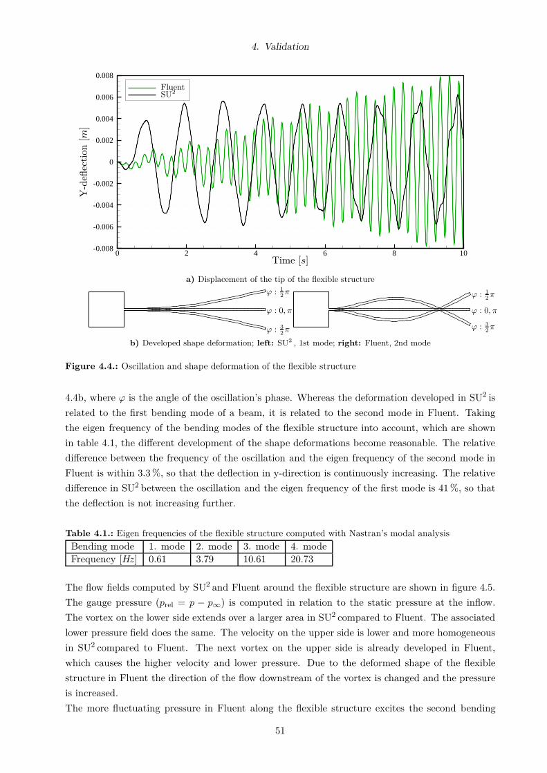
4. Validation
0 2 4 6 8 10-0.008
-0.006
-0.004
-0.002
0
0.002
0.004
0.006
0.008
Time [s]
Y-d
eflec
tion
[m]
FluentSU2
a) Displacement of the tip of the flexible structure
ϕ : 0, π
ϕ : 12π
ϕ : 32π
ϕ : 0, π
ϕ : 12π
ϕ : 32π
b) Developed shape deformation; left: SU2 , 1st mode; right: Fluent, 2nd mode
Figure 4.4.: Oscillation and shape deformation of the flexible structure
4.4b, where ϕ is the angle of the oscillation’s phase. Whereas the deformation developed in SU2 is
related to the first bending mode of a beam, it is related to the second mode in Fluent. Taking
the eigen frequency of the bending modes of the flexible structure into account, which are shown
in table 4.1, the different development of the shape deformations become reasonable. The relative
difference between the frequency of the oscillation and the eigen frequency of the second mode in
Fluent is within 3.3 %, so that the deflection in y-direction is continuously increasing. The relative
difference in SU2 between the oscillation and the eigen frequency of the first mode is 41 %, so that
the deflection is not increasing further.
Table 4.1.: Eigen frequencies of the flexible structure computed with Nastran’s modal analysis
Bending mode 1. mode 2. mode 3. mode 4. mode
Frequency [Hz] 0.61 3.79 10.61 20.73
The flow fields computed by SU2 and Fluent around the flexible structure are shown in figure 4.5.
The gauge pressure (prel = p − p∞) is computed in relation to the static pressure at the inflow.
The vortex on the lower side extends over a larger area in SU2 compared to Fluent. The associated
lower pressure field does the same. The velocity on the upper side is lower and more homogeneous
in SU2 compared to Fluent. The next vortex on the upper side is already developed in Fluent,
which causes the higher velocity and lower pressure. Due to the deformed shape of the flexible
structure in Fluent the direction of the flow downstream of the vortex is changed and the pressure
is increased.
The more fluctuating pressure in Fluent along the flexible structure excites the second bending
51

4. Validation
mode. The longer extension of an homogenous pressure field along both sides of the structure in
SU2 is more synchronised with the first bending mode. As the flow field and the shape deformation
of the flexible structure have an influence on each other, the transient flow field with a rigid structure
needs to be examined in order to identify the reason for the different results of Fluent and SU2 in
figure 4.4a.
: -0.11 -0.074 -0.038 -0.002 0.034 0.07Rel Pressure [Pa]
a) SU2
b) Fluent
Figure 4.5.: Pressure distribution around flexible structure, vectors represent velocity components
Figure 4.6 shows the oscillation of the pressure at a control point due to the Kármán vortex street
downstream of the square applying an rigid structure, where figure 4.6a shows the location of
the control point and figure 4.6b its pressure oscillation. The oscillation of the pressure indicates
the frequency of the vortices. As can be seen the frequency of the pressure oscillation is higher
computed by Fluent compared to SU2 . The oscillation’s frequency of SU2 is 4.48 times smaller
than Fluent’s (SU2: 0.89 Hz, Fluent: 3.99 Hz), matching to the differences in the oscillation of the
flexible structure in figure 4.4a. The frequency of the Kármán vortex street in Fluent is higher,
which leads to the quicker change of pressure and therefore the shape deformation (second bending
mode). As the frequency is close to the eigen frequency of the second bending mode its development
is further supported. The frequency of the Kármán vortex street is smaller in SU2 , which results
52

4. Validation
c
c c12c
Control point
a) Location of the control point
0 0.5 1 1.5 2
-0.07
-0.06
-0.05
-0.04
-0.03
-0.02
-0.01
0
Time [s]R
elati
ve
Pre
ssure
[Pa]
SU2
Fluent
b) Pressure oscillation at control point
Figure 4.6.: Oscillation of the pressure due to the Kármán vortex street downstream of the square with anrigid structure
in the more homogenous pressure field along the structure, resulting in the bending mode of first
order - again supported by the eigen frequency, which is close to the vortex frequency.
In accordance to Roshko (1961) the Strouhal number can be approximated with St = 0.2 for a
cylinder for a wide range of the Reynolds number: 1.5 · 102 < Re < 106. The Reynolds number
is Re = 204 and in this range. The definition of the Strouhal number is used to compute the
frequency:
f =St · v
L= 6.3 Hz (4.1)
It has to be taken into account that the approximation of the Strouhal number is valid for a cylinder
and not a square. Also, the influence of the structure downstream of the square is not considered
within the definition of the Strouhal number, however, the computed frequency is more similar to
the frequency computed by Fluent (f = 3.99 Hz) rather than SU2 (f = 0.89 Hz).
It has been shown that the different developed oscillations of the flexible structure are related to a
different flow solution computed by the solvers and not to the implementation of the code adapter.
The different behavior is, however, examined further. The oscillation is influenced by the material
properties of the flexible structure and the pressure distribution due to the Kármán vortex street.
The vortex street depends on the Reynolds number, which is varied in section 4.1.1. The effect of
the variation of the structure’s mass is analysed in section 4.1.2.
4.1.1. Variation of Reynolds Number
For the analysis of the effect due to a variation of the Reynolds number two additional cases are
considered. For the first case the Reynolds number is reduced to 75 % and for the second it is
53

4. Validation
raised to 200 % of the original (Re = 204). The Reynolds number is changed by varying the inflow
velocity. The pressure oscillation at the control point (shown in figure 4.6a) due to the Kármán
vortex street using a rigid structure downstream of the square is shown in figure 4.7.
0 0.2 0.4 0.6 0.8 1 1.2 1.4
-0.4
-0.3
-0.2
-0.1
0
Time [s]
Rel
.P
ress
ure
[Pa]
Org. Re
0.75 Re
2 Re
a) Fluent
0 0.2 0.4 0.6 0.8 1 1.2 1.4
-0.4
-0.3
-0.2
-0.1
0
Time [s]
Rel
.P
ress
ure
[Pa]
b) SU2
Figure 4.7.: Pressure oscillation at control point for varied Reynold numbers
Applying the different Reynold numbers lead to the frequencies of the pressure oscillation shown in
table 4.2. The change of the frequencies are adequate proportional to the change of the Reynolds
number.
Table 4.2.: Frequencies of the pressure oscillation for different Reynolds numbers
Frequency [Hz]Reynolds number Fluent SU2
0.75 · Reorg 2.94 0.70Reorg 3.99 0.89
2 · Reorg 7.78 1.73
Running coupled simulations with the initial solution of the different Reynold numbers in Fluent
and SU2 results in a different behavior of the structure’s oscillation, which is shown in figure 4.8. The
higher Reynolds number results (in Fluent) in a pressure oscillation’s frequency between the eigen
frequencies of the second and third mode (compare tables 4.2 and 4.1). In the coupled simulation
the flexible structure oscillates with an mixture of the second and third mode, which can be seen
in figure 4.8a (combined higher and smaller frequency of the oscillation). The deflection of the tip
does not increase further within the simulated time, which is related to the greater distance to the
natural frequencies. The higher Reynolds number in SU2 results in an frequency of the pressure
oscillation between the first and the second mode. Within the first five seconds of the coupled
simulation the flexible structure oscillates irregular with a mixture of first and second mode. The
fluid-structure interaction produces after an regular oscillation with an frequency of 3.81 Hz and
the deformation type similar to the second bending mode. The relative difference is with 0.35 %
very close to the second mode so that the deflection of the structure’s tip is increasing further.
54

4. Validation
0 1 2 3 4 5 6 7 8 9 10-0.015
-0.01
-0.005
0
0.005
0.01
0.015
Time [s]
Y-d
eflec
tion
[m]
Org. Re
0.75 Re2 Re
a) Fluent
0 1 2 3 4 5 6 7 8 9-0.015
-0.01
-0.005
0
0.005
0.01
0.015
Time [s]
Y-d
eflec
tion
[m]
b) SU2
Figure 4.8.: Oscillation of the structure’s tip for varied Reynold numbers
The result of the coupled simulation applying the lower Reynolds number in Fluent is an oscillation
of the structure with an mixture of the first and second mode in the beginning. The fluid-structure
interaction results after in an increasing oscillation being related to the first bending mode with an
frequency of 0.81 Hz. The relative difference of 32.87 % to the eigen frequency of the first mode is
small enough for an increase of the oscillation (41 % in the original case in SU2 was too large for
an increase). The lower Reynolds number in SU2 is very close to the natural frequency so that the
first mode develops and increases with an frequency of 0.73 Hz (relative difference to the natural
frequency of the first mode: 20.65 %).
4.1.2. Variation of Mass
For the analysis of the effects due to a variation of the mass of the flexible structure two additional
cases are considered. For the first case the density is reduced to 25 % and for the second it is raised
to 150 %. The eigen frequencies are reduced or increased in accordance to the change of mass as
shown in table 4.3.
55

4. Validation
Table 4.3.: Eigen frequencies of the flexible structure with varied density
Eigen frequency [Hz]Simulation Case 1. Mode 2. Mode 3. Mode 4. Mode
0.25 · ρorg 1.21 7.59 21.21 41.46ρorg 0.61 3.79 10.61 20.73
1.5 · ρorg 0.49 3.10 8.66 16.93
Figure 4.9 shows the oscillation of the structure’s tip for the different masses used for the coupled
simulation. The shapes of the deformation developing during the oscillation can not be explained
with the frequency of the pressure oscillation (due to the vortex street) being close or not to any
natural frequency. Changing the mass of the structure seems to reduce the influence of the eigen
frequency and to increase therefore the influence of other effects on the oscillation of the flexible
structure i.e. the inertia. The lower mass reduces the inertia of the structure, which increases the
influence of the force due to the pressure resulting in an higher motion of the structure compared
to the structure with the same external force and an higher inertia.
0 1 2 3 4 5 6 7 8 9 10-0.02
-0.01
0
0.01
0.02
Time [s]
Y-d
eflec
tion
[m]
morg
0.25 morg
1.5 morg
a) Fluent
0 1 2 3 4 5 6 7 8 9 10-0.02
-0.01
0
0.01
0.02
Time [s]
Y-d
eflec
tion
[m]
b) SU2
Figure 4.9.: Oscillation of the structure’s tip for varied masses of the structure
56
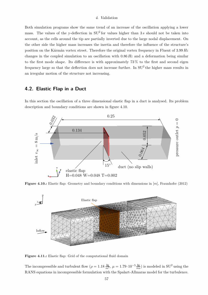
4. Validation
Both simulation programs show the same trend of an increase of the oscillation applying a lower
mass. The values of the y-deflection in SU2 for values higher than 3 s should not be taken into
account, as the cells around the tip are partially inverted due to the large nodal displacement. On
the other side the higher mass increases the inertia and therefore the influence of the structure’s
position on the Kármán vortex street. Therefore the original vortex frequency in Fluent of 3.99 Hz
changes in the coupled simulation to an oscillation with 0.86 Hz and a deformation being similar
to the first mode shape. Its difference is with approximately 73 % to the first and second eigen
frequency large so that the deflection does not increase further. In SU2 the higher mass results in
an irregular motion of the structure not increasing.
4.2. Elastic Flap in a Duct
In this section the oscillation of a three dimensional elastic flap in a duct is analysed. Its problem
description and boundary conditions are shown in figure 4.10.
pre
ssure
outl
etp
=0
0.25
H=0.048 W=0.048 T=0.002elastic flap
0.134
0.03
2
0.05
20.
064
duct (no slip walls)15◦
inle
tv ∞
=8
m/s
Figure 4.10.: Elastic flap: Geometry and boundary conditions with dimensions in [m], Fraunhofer (2012)
x
y
z
Inflow
Elastic flap
Figure 4.11.: Elastic flap: Grid of the computational fluid domain
The incompressible and turbulent flow (ρ = 1.18 kgm3 , µ = 1.79 ·10−5 kg
ms) is modeled in SU2 using the
RANS equations in incompressible formulation with the Spalart-Allmaras model for the turbulence.
57

4. Validation
The grid of the computational fluid domain is shown in figure 4.11, which is the same for SU2 and
Fluent.
x
y
zNastranFluent, SU2
Control point
Figure 4.12.: Elastic flap: Coupled surface grids ofthe CFD and FEM domains
The CFD grid contains 24811 tetrahedral ele-
ments with 5691 nodes, whereas the FEM grid
consists of 800 brick elements with 1323 nodes.
The equations are discretised in space with an
scheme of first order. Figure 4.12 shows the
coupled surface grids of the CFD and FEM do-
mains.
The elastic flap is modeled with a linear elas-
tic material with the density ρ = 1000 kgm3 , the
Young’s modulus E = 108Pa and the Poisson’s
ratio ν = 0.49. The transient simulation is dis-
cretised with an scheme of first order with a
time step size of ∆t = 0.25 ms. The simulation
time is set to 0.2 s. During the coupled simula-
tion the relative wall force and the nodal posi-
tion are exchanged. Also the time step size used
in SU2 is sent to Nastran. As the current ver-
sion of SU2 does not support an adaptive time
step size it remains constant during the entire simulation. At the inlet the mass flow is defined
with a velocity of v = 8 ms . At the outlet the gauge pressure is set to zero and the elastic flap is
modeled as a no slip wall. In Nastran the elastic flap is constraint at the top.
0 0.05 0.1 0.15 0.2
-0.008
-0.006
-0.004
-0.002
0
0.002
SU2
Fluent
Time [s]
X-D
ispla
cem
ent
[m]
Figure 4.13.: Oscillation of the control point of theelastic flap
A control point, which is shown in figure 4.12, is
used to track the oscillation of the elastic flap in
the duct due to the fluid-structure interaction.
The oscillation of the flap is shown in figure
4.13 for the coupled simulation with Fluent and
SU2 . The displacement of the control point in
x-direction is shown over the time. The CFD
solvers develop different solutions. Whereas the
amplitude decreases in the coupled simulation
with Fluent, it increases with SU2 . The first
displacement of the flap is larger in Fluent. The
frequencies of the oscillation is the same in both
simulations.
In order to find the reason for the different de-
veloped solutions the z-plane (compare coordi-
nate system in figure 4.11) in the middle of the
duct is analysed. Figure 4.14 shows the relative
pressure for different time steps. The time steps
58
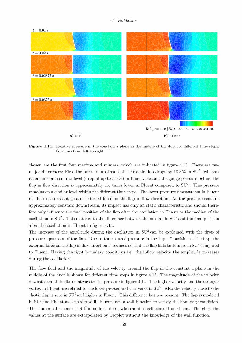
4. Validation
t = 0.01 s
t = 0.02 s
t = 0.02875 s
t = 0.0375 s
a) SU2
: -230 -84 62 208 354 500Rel pressure [Pa]
b) Fluent
Figure 4.14.: Relative pressure in the constant z-plane in the middle of the duct for different time steps;flow direction: left to right
chosen are the first four maxima and minima, which are indicated in figure 4.13. There are two
major differences: First the pressure upstream of the elastic flap drops by 18.3 % in SU2 , whereas
it remains on a similar level (drop of up to 3.5 %) in Fluent. Second the gauge pressure behind the
flap in flow direction is approximately 1.5 times lower in Fluent compared to SU2 . This pressure
remains on a similar level within the different time steps. The lower pressure downstream in Fluent
results in a constant greater external force on the flap in flow direction. As the pressure remains
approximately constant downstream, its impact has only an static characteristic and should there-
fore only influence the final position of the flap after the oscillation in Fluent or the median of the
oscillation in SU2 . This matches to the difference between the median in SU2 and the final position
after the oscillation in Fluent in figure 4.13.
The increase of the amplitude during the oscillation in SU2 can be explained with the drop of
pressure upstream of the flap. Due to the reduced pressure in the “open” position of the flap, the
external force on the flap in flow direction is reduced so that the flap falls back more in SU2 compared
to Fluent. Having the right boundary conditions i.e. the inflow velocity the amplitude increases
during the oscillation.
The flow field and the magnitude of the velocity around the flap in the constant z-plane in the
middle of the duct is shown for different time steps in figure 4.15. The magnitude of the velocity
downstream of the flap matches to the pressure in figure 4.14. The higher velocity and the stronger
vortex in Fluent are related to the lower presser and vice versa in SU2. Also the velocity close to the
elastic flap is zero in SU2 and higher in Fluent. This difference has two reasons. The flap is modeled
in SU2 and Fluent as a no slip wall. Fluent uses a wall function to satisfy the boundary condition.
The numerical scheme in SU2 is node-centred, whereas it is cell-centred in Fluent. Therefore the
values at the surface are extrapolated by Tecplot without the knowledge of the wall function.
59

4. Validation
t = 0.01 s
t = 0.02 s
a) SU2
: 0 6.2 12.4 18.6 24.8 31Velocity [ m
s]
b) Fluent
Figure 4.15.: Flow field in the constant z-plane in the middle of the duct for different time steps
0 0.05 0.1 0.15 0.2
-0.008
-0.006
-0.004
-0.002
0
0.002
Time [s]
X-D
ispla
cem
ent
[m]
vorg
0.75 vorg
0.5 vorg
Figure 4.16.: Oscillation of the control point of the elasticflap for different inflow velocities in SU2
In order to examine the fluid-structure in-
teraction a bit further in SU2 , the mag-
nitude of the velocity at the inflow is var-
ied. Two additional cases are considered
with a reduced inflow velocity to 75 % and
50 % of the original speed (vorg = 8 ms ).
The oscillation of the control point of the
elastic flap is shown in figure 4.16. Re-
ducing the inflow speed has some effects
on the oscillation. The magnitude of the
oscillation’s median is reduced for a lower
inflow velocity, which is reasonable as the
external static force on the flap is reduced.
Also the amplitude does not increase, if the
velocity is reduced to 50 %. The increase
of the amplitude for 75 % of the original
velocity is negligible within the simulated
time. The frequency of the oscillation is
increased slightly.
The variation of the inflow velocity showed that it has not the major influence on the increase or
decrease of the amplitude. This behavior is based on the drop of pressure in SU2 whenever the flap
“opens”.
60
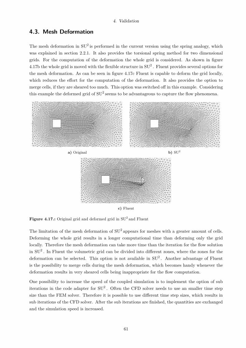
4. Validation
4.3. Mesh Deformation
The mesh deformation in SU2 is performed in the current version using the spring analogy, which
was explained in section 2.2.1. It also provides the torsional spring method for two dimensional
grids. For the computation of the deformation the whole grid is considered. As shown in figure
4.17b the whole grid is moved with the flexible structure in SU2 . Fluent provides several options for
the mesh deformation. As can be seen in figure 4.17c Fluent is capable to deform the grid locally,
which reduces the effort for the computation of the deformation. It also provides the option to
merge cells, if they are sheared too much. This option was switched off in this example. Considering
this example the deformed grid of SU2 seems to be advantageous to capture the flow phenomena.
-0.02 0 0.02 0.04 0.06
2
1
0
1
2
a) Original
-0.02 0 0.02 0.04 0.06
b) SU2
-0.02 0 0.02 0.04 0.06
2
1
0
1
2
c) Fluent
Figure 4.17.: Original grid and deformed grid in SU2 and Fluent
The limitation of the mesh deformation of SU2 appears for meshes with a greater amount of cells.
Deforming the whole grid results in a longer computational time than deforming only the grid
locally. Therefore the mesh deformation can take more time than the iteration for the flow solution
in SU2 . In Fluent the volumetric grid can be divided into different zones, where the zones for the
deformation can be selected. This option is not available in SU2 . Another advantage of Fluent
is the possibility to merge cells during the mesh deformation, which becomes handy whenever the
deformation results in very sheared cells being inappropriate for the flow computation.
One possibility to increase the speed of the coupled simulation is to implement the option of sub
iterations in the code adapter for SU2 . Often the CFD solver needs to use an smaller time step
size than the FEM solver. Therefore it is possible to use different time step sizes, which results in
sub iterations of the CFD solver. After the sub iterations are finished, the quantities are exchanged
and the simulation speed is increased.
61
5. Summary and Outlook
The development of the code adapter to couple SU2 v2.0 with MpCCI in order to perform aeroelastic
simulations was described in this work. The application programming interface (API) of MpCCI,
to be used in the language C, has been used to exchange information with SU2 , which is written
using the language C++. In order to minimise the effort for the integration of the code adapter on
other computer systems, “transfer functions” were developed, which are called by SU2 at run time.
These functions manipulate the data i.e. the coupled grid and the pressure of SU2 and store them
in global structures, which are accessible by the API of MpCCI. Once the exchange of quantities
is accomplished by MpCCI, the transfer functions apply the nodal displacements computed by the
partner code e.g. Nastran and deform the SU2 grid. To use the developed code adapter only some
simple calls of these functions need to be added in the original SU2 files reducing the necessary
changes to a minimum. A detailed instruction for the integration of the code adapter is given in
the appendix.
The code adapter has been validated using a two-dimensional and a three-dimensional test cases. In
the first case a thin-walled structure is excited to oscillate due to a Kármán vortex street, whereas
in the latter case an elastic flap blocking the flow in a duct starts to oscillate. Both cases have been
investigated with SU2 and Fluent - each coupled with Nastran. Although the results differ it has
been shown the developed code adapter is working properly as the changes are related to the flow
solution itself and not the coupling.
The Kármán vortex street developing due to a square in SU2 is a fifth is a 4.48 of the frequency
in Fluent in an uncoupled transient simulation. Therefore different bending modes are excited in
a coupled simulation with Nastran and the structure’s tip oscillates with a frequency 4.3 times
smaller in SU2 compared to Fluent.
The oscillation of the elastic flaps decreases in a coupled simulation with Fluent, whereas it in-
creases with SU2 . It was shown the changes result from a different pressure field. As the pressure
upstream of the flap drops approximately 13.3 % in SU2 and only 3.5 % in Fluent whenever the flap
“opens”, the oscillation in SU2 is excited. Also, the vortex downstream the flap is stronger and
the corresponding pressure lower in all time steps in Fluent compared to SU2 , which increases the
static force in flow direction and therefore the displacement of the flap in Fluent.
The developed code adapter is capable to compute and send the (relative) wall force to MpCCI
and receive and apply the nodal displacements. It is also able to send the time step size used in
SU2 in transient simulations. The coupling scheme is limited to schemes, where SU2 exchanges the
coupled quantities after each iteration step. It appears appropriate to improve the code adapter
further: The code adapter should be extended for parallel simulations. As the bottleneck related
to the simulation speed is the grid deformation of SU2 , the option of sub iterations for SU2 in a
coupled simulation should be implemented to reduce the exchange of quantities to a minimum.
62
Bibliography
Acikgoz, N. and Bottasso, C. (2007). A unified approach to the deformation of simplicial and non-
simplicial meshes in two and three dimensions with guaranteed validity. Computers & Structures,
85:944–954.
Appa, K. (1989). Finite-surface spline. Journal of Aircraft, 26(5):495–496.
Beckert, A. and Wendland, H. (2001). Multivariate interpolation for fluid-structure-interaction
problems using radial basis functions. Aerospace Science and Technology, 5:125–131.
Bendiksen, O. (2004). Modern developments in aeroelasticity. Proceedings of the Institute of
Mechanical Engineers Part G: Journal of Aerospace Engineering, 218:157–177.
Bos, F. M., v. Oudheusden, B. W., and Bijl, H. (2013). Radial basis function based mesh defor-
mation applied to simulation of flow around flapping wings. Computers and Fluids, 79:167–177.
Bottasso, C. L., Detomi, D., and Serra, R. (2005). The ball-vertex method: A new simple spring
analogy method for unstructured dynamic meshes. Computer Methods in Applied Mechanics and
Engineering, 194:4244–4264.
Chen, P. and Jadic, I. (1998). Interfacing of fluid and structural models via innovative structural
boundary element method. AIAA Journal, 36(2):282–287.
Degand, C. and Farhat, C. (2002). A three-dimensional torsional spring analogy method for un-
structured dynamic meshes. Computers and Structures, 80:305–316.
Farhat, C., Geuzaine, P., and Brown, G. (2003). Application of a three-field nonlinear fluid-structure
formulation to the prediction of the aeroelastic parameters of an f-16 fighter. Computers and
Fluids, 32:3–29.
Fraunhofer (2012). MpCCI 4.2.1-3 Documentation. Fraunhofer Institute for Algorithms and Sci-
entific Computing SCAI.
Goura, G. (2001). Time Marching Analysis of Flutter using Computational Fluid Dynamics. PhD
thesis, University of Glasgow.
Guruswamy, G. and Byun, C. (1995). Direct coupling of euler flow equations with plate finite
element structures. AIAA Journal, 33(2):375–377.
Harder, R. and Desmarais, R. (1972). Interpolation using surface splines. Journal of Aircraft,
9(2):189–191.
63

Bibliography
Hübner, B., Walhorn, E., and Dinkler, D. (2004). A monolithic approach to fluid-structure interac-
tion using space-time finite elements. Computer Methods in Applied Mechanics and Engineering,
193:2087–2104.
Hirsch, C. (2007). Numerical Computation of Internal and External Flows: The Fundamentals of
Computational Fluid Dynamics. Butterworth-Heinemann.
Kitware, I. (2010). VTK User’s Guide. Kitware, Inc. 11th Edition.
Liu, Y., Guo, Z., and Liu, J. (2012). Rbfs-msa hybrid method for mesh deformation. Chinese
Journal of Aeronautics, 25:500–507.
Lombardi, M., Parolini, N., and Quarteroni, A. (2013). Radial basis functions for inter-grid inter-
polation and mesh motion in fsi problems. Computational Methods in Applied Mechanics and
Engineering, 256:117–131.
Luke, E., Collins, E., and Blades, E. (2012). A fast mesh deformation method using explicit
interpolation. Journal of Computational Physics, 231:586–601.
Palacios, F., Colonno, M. R., Aranake, A. C., Campos, A., Copeland, S. R., Economon, T. D.,
Lonkar, A. K., Lukaczyk, T. W., Taylor, T. W. R., and Alonso, J. J. (2013). Stanford university
unstructured (SU2): An open-source integrated computational environment for multi-physics
simulation and design. In 51st AIAA Aerospace Sciences Meeting including the New Horizons
Forum and Aerospace Exposition.
Rampurawala, A. (2006). Aeroelastic Analysis of Aircraft with Control Surfaces using CFD. PhD
thesis, University of Glasgow.
Rendall, T. C. S. and Allen, C. B. (2008). Unified fluid-structure interpolation and mesh mo-
tion using radial basis functions. International Journal for Numerical Methods in Engineering,
74:1519–1559.
Roshko, A. (1961). Experiments on the flow past a circular cylinder at very high reynolds number.
Journal of Fluid Mechanics, 10(3):345–356.
Sadeghi, M., Lui, F., Lai, K., and Tsai, H. (2004). Application of three-dimensional interfaces
for data transfer in aeroelastic computations. In 22nd Applied Aerodynamics Conference and
Exhibit, number 2004-5376.
Schwartz, R. L., Phoenix, T., and Foy, B. D. (2005). Learning Perl. O’Reilly, 4th edition.
Smith, M., Hodges, D., and Cesnik, C. (1995). An evaluation of computational algorithms to
interface between cfd and csd methodologies. Technical report, WL-TR-96-3055, U.S. Air Force
Research Lab.
Swift, A. (2011). Simulation of Aircraft Aeroelasticity. PhD thesis, University of Liverpool.
Wendland, H. (1996). Konstruktion und Untersuchung radialer Basisfunktionen mit kompaktem
Träger. PhD thesis, Universität Göttingen.
64

Bibliography
Woodgate, M., Badcock, K., Rampurawala, A., Richards, B., Nardini, D., and Henshaw, M. (2005).
Aeroelastic calculations for the hawk aircraft using the euler equations. Journal of Aircraft,
40(4):1005–1012.
Zhou, X. and Li, S. (2013). A new mesh deformation method based on disk relaxation algorithm
with pre-displacement and post-smoothing. Journal of Computational Physics, 235:199–215.
65
List of Figures
2.1. Typical cycle for partitioned approach . . . . . . . . . . . . . . . . . . . . . . . . . . 2
2.2. Boundary element method: treatment of an airfoil, Rampurawala (2006) . . . . . . . 6
2.3. Constant Volume Tetrahedron, Woodgate et al. (2005) . . . . . . . . . . . . . . . . . 8
2.4. left: Collapse mechanism; right: Ball-vertex spring method . . . . . . . . . . . . . . 11
2.5. Added faces in torsional spring method, Bottasso et al. (2005) . . . . . . . . . . . . . 11
2.6. Architecture of MpCCI, Fraunhofer (2012) . . . . . . . . . . . . . . . . . . . . . . . . 12
2.7. Association between node and element, Fraunhofer (2012) . . . . . . . . . . . . . . . 13
2.8. Parameters to control the neighborhood search in MpCCI , Fraunhofer (2012) . . . . 14
2.9. Coupling algorithm with SU2 exchanging after iteration and NASTRAN before . . . 15
3.1. API between SU2 and MpCCI . . . . . . . . . . . . . . . . . . . . . . . . . . . . . . . 16
3.2. MpCCI GUI: Model step (1) . . . . . . . . . . . . . . . . . . . . . . . . . . . . . . . 17
3.3. Setup in the GUI of MpCCI . . . . . . . . . . . . . . . . . . . . . . . . . . . . . . . . 18
3.4. Activity diagram of the scanner script . . . . . . . . . . . . . . . . . . . . . . . . . . 20
3.5. MpCCI GUI: Coupling step (2) . . . . . . . . . . . . . . . . . . . . . . . . . . . . . . 20
3.6. Structure of the code adapter. Black and blue arrows denote communication and
exchange of data. . . . . . . . . . . . . . . . . . . . . . . . . . . . . . . . . . . . . . . 22
3.7. Class hierarchy in SU2_CFD, Palacios et al. (2013) . . . . . . . . . . . . . . . . . . 23
3.8. Classes and dual-grid used by SU2_CFD for the geometry processing, Palacios et al.
(2013) . . . . . . . . . . . . . . . . . . . . . . . . . . . . . . . . . . . . . . . . . . . . 23
3.9. Fraction of the classes related to the class CSolution, Palacios et al. (2013) . . . . . 24
3.10. Main activities in function “main” of SU2_CFD . . . . . . . . . . . . . . . . . . . . 25
3.11. Interaction between SU2 and MpCCI during the exchange of the quantities; The star
indicates a pointer to the quantity . . . . . . . . . . . . . . . . . . . . . . . . . . . . 26
3.12. Data structure for functions involved during the data exchange between SU2 and
MpCCI . . . . . . . . . . . . . . . . . . . . . . . . . . . . . . . . . . . . . . . . . . . 27
3.13. Sequence during coupling initialisation; blue: reference to the paragraphs . . . . . . 29
3.14. Sequence during exchange of data; blue: reference to the paragraphs . . . . . . . . . 40
3.15. Normal vector computation of surface grids in SU2 . . . . . . . . . . . . . . . . . . . 42
3.16. Equivalence of applying the forces on a thin plate . . . . . . . . . . . . . . . . . . . . 42
3.17. Sequence during finalisation of coupling by SU2 . . . . . . . . . . . . . . . . . . . . . 48
4.1. Vortex-induced vibration: Geometry and boundary conditions with dimensions in
cm, Fraunhofer (2012) . . . . . . . . . . . . . . . . . . . . . . . . . . . . . . . . . . . 49
4.2. Vortex-induced vibration: Grid of fluid domain and flexible structure. Black: SU2 and
Fluent, green: Nastran . . . . . . . . . . . . . . . . . . . . . . . . . . . . . . . . . . . 50
66

List of Figures
4.3. Initial condition used for the coupled simulation: Magnitude of velocity . . . . . . . 50
4.4. Oscillation and shape deformation of the flexible structure . . . . . . . . . . . . . . . 51
4.5. Pressure distribution around flexible structure, vectors represent velocity components 52
4.6. Oscillation of the pressure due to the Kármán vortex street downstream of the square
with an rigid structure . . . . . . . . . . . . . . . . . . . . . . . . . . . . . . . . . . . 53
4.7. Pressure oscillation at control point for varied Reynold numbers . . . . . . . . . . . 54
4.8. Oscillation of the structure’s tip for varied Reynold numbers . . . . . . . . . . . . . . 55
4.9. Oscillation of the structure’s tip for varied masses of the structure . . . . . . . . . . 56
4.10. Elastic flap: Geometry and boundary conditions with dimensions in [m], Fraunhofer
(2012) . . . . . . . . . . . . . . . . . . . . . . . . . . . . . . . . . . . . . . . . . . . . 57
4.11. Elastic flap: Grid of the computational fluid domain . . . . . . . . . . . . . . . . . . 57
4.12. Elastic flap: Coupled surface grids of the CFD and FEM domains . . . . . . . . . . 58
4.13. Oscillation of the control point of the elastic flap . . . . . . . . . . . . . . . . . . . . 58
4.14. Relative pressure in the constant z-plane in the middle of the duct for different time
steps; flow direction: left to right . . . . . . . . . . . . . . . . . . . . . . . . . . . . . 59
4.15. Flow field in the constant z-plane in the middle of the duct for different time steps . 60
4.16. Oscillation of the control point of the elastic flap for different inflow velocities in SU2 60
4.17. Original grid and deformed grid in SU2 and Fluent . . . . . . . . . . . . . . . . . . . 61
B.1. Copy first part from “Copy_to_SU2_CFD.cpp” into “SU2_CFD.cpp” . . . . . . . . 71
B.2. Copy second part from “Copy_to_SU2_CFD.cpp” into “SU2_CFD.cpp” . . . . . . 72
B.3. Copy third part from “Copy_to_SU2_CFD.cpp” into “SU2_CFD.cpp” . . . . . . . 72
67

A. Appendix
Table A.1.: Codes in Perl for regular expressions
Code Meaning
/ <Regular expression> / Match regular expression to a string\w Alphanumeric character\s White space\d Digit\% %\( (\\ \̂ At the beginning of a string∗ Zero or more occurrences+ One or more occurrences[ <Set of items> ] Match any item in the set( <Expression> ) Tag expression
Listing A.1: Structs of MpCCI used during initialisation and data exchange
// mpcci_types . htypedef struct _MPCCI_PART MPCCI_PART;struct _MPCCI_PART {
char ∗name ;MPCCI_QUANT ∗ quants ;int pid ;int nnodes ;int nelems ;unsigned c sy s ;/∗ . . . ∗/
}#define MPCCI_PART_NAME(_p) ( (_p)−>name )/∗ . . . ∗/typedef struct _MPCCI_QUANT MPCCI_QUANT;struct _MPCCI_QUANT {
int qid ;int smethod ;/∗ . . . ∗/
}
68

A. Appendix
Listing A.2: Structs of MpCCI used during initialisation
// mpcci_types . htypedef struct _MPCCI_TINFO MPCCI_TINFO;struct _MPCCI_TINFO {
int mpcci_state ;int mpcci_used ;int i t e r ;double time ;double dt ;/∗ . . . ∗/
}typedef struct _MPCCI_CINFO MPCCI_CINFO;struct _MPCCI_CINFO {
const char ∗codename ;double time ;int i t e r ;int n c l i e n t s ;int nprocs ;/∗ . . . ∗/
}typedef struct _MPCCI_JOB MPCCI_JOB;struct _MPCCI_JOB {
MPCCI_SERVER ∗ s e r v e r s ;/∗ . . . ∗/
}typedef struct _MPCCI_DRIVER MPCCI_DRIVER;struct _MPCCI_DRIVER {
void (∗ a f t e rC los eSetup ) ( void ) ;int (∗ partUpdate ) ( /∗ . . . ∗/ ) ;int (∗ de f in ePar t ) ( /∗ . . . ∗/ ) ;int (∗ getFaceNodeValues ) ( /∗ . . . ∗/ ) ;int (∗ getGlobValues ) ( /∗ . . . ∗/ ) ;void (∗ putFaceNodeValues ) ( /∗ . . . ∗/ ) ;/∗ . . . ∗/
}
// adapter . cstat ic MPCCI_TINFO mpcciTinfo = {0};stat ic MPCCI_JOB ∗mpcciJob = NULL;stat ic MPCCI_DRIVER MpCCIDriverFunctions = {
/∗ . . . ∗/ ,MpCCI_Driver_afterCloseSetup ,NULL,/∗ . . . ∗/MpCCI_Driver_partUpdate ,/∗ . . . ∗/
} ;
69

B. Instruction for Code Adapter Integration
The following sections describe how to integrate the code adapter into you version of SU2 with
Linux. The code adapter was developed for MpCCI v.4.2.1-3 and SU2 v2.0. For other versions
changes might be necessary within the C++ and C files.
B.1. Adapt the C++ Files
1. Create the folder “MpCCI_Adapter” within your SU2 path:
<...>/SU2v2.0/trunk/MpCCI_Adapter/
2. Copy the following source and header files into the created directory “MpCCI_Adapter/”:
· adapter.c
· adapter.h
· transfer.cpp
· transfer.hpp
3. Open the file “adapter.h” and adapt the path to include the header file “mpcci.h” in accordance
to your file system as shown in listing B.1.
Listing B.1: Inclusion of “mpcci.h”
// adapter . h
#include ‘ ‘ <.. . >/MpCCI/4 . 2 . 1/ include/mpcci . h ’ ’
4. If you have not modified the files “SU2_CFD.hpp” and “SU2_CFD.cpp” (and are using
SU2 v2.0) simply replace the originals with the corresponding files provided and continue with
section B.2. The original files to be replaced are located in:
<...>/SU2v2.0/trunk/SU2_CFD/src/SU2_CFD.cpp
<...>/SU2v2.0/trunk/SU2_CFD/include/SU2_CFD.hpp
Continue with the next step, if you have modified the original files “SU2_CFD.hpp” and “SU2_CFD.cpp”
or if you are not using SU2 v2.0.
70

B. Instruction for Code Adapter Integration
4.a If you have modified the “SU2_CFD.hpp” and “SU2_CFD.cpp”, you have to adapt them
individually. Open the original file “SU2_CFD.hpp” and include the header file “transfer.hpp” as
shown in listing B.2.
Listing B.2: Inclusion of “transfer.hpp”
//SU2_CFD. hpp
#include ‘ ‘ . . / . . / MpCCI_Adapter/ t r a n s f e r . hpp ’ ’
4.b Open the provided file “Copy_to_SU2_CFD.cpp” and copy it lines into the original file
“SU2_CFD.cpp” as explicated below. The line numbers in the figures might vary.
4.b.1 Copy the the first part of “Copy_to_SU2_CFD.cpp” into “SU2_CFD.cpp” before the
iteration loop starts and after the convergence history file is opened as shown in figure B.1.
Figure B.1.: Copy first part from “Copy_to_SU2_CFD.cpp” into “SU2_CFD.cpp”
4.b.2 Copy the the second part of “Copy_to_SU2_CFD.cpp” into “SU2_CFD.cpp” before the
solution output is written and after the convergence criteria are checked as shown in figure B.2.
4.b.3 Copy the the third part of “Copy_to_SU2_CFD.cpp” into “SU2_CFD.cpp” before the
final MPI parallelisation is performed and after the convergence history file is closed as shown in
figure B.3.
71

B. Instruction for Code Adapter Integration
Figure B.2.: Copy second part from “Copy_to_SU2_CFD.cpp” into “SU2_CFD.cpp”
Figure B.3.: Copy third part from “Copy_to_SU2_CFD.cpp” into “SU2_CFD.cpp”
72

B. Instruction for Code Adapter Integration
B.2. Adapt the Make Files
5. Adapt the make files “Makefile.am” and “Makefile.in” located in
<...>/SU2v2.0/trunk/SU2_CFD/bin/
to include the following files:
· adapter.c
· adapter.h
· transfer.cpp
· transfer.hpp
Pay attention to use the correct path when including the files. The object files used for the
compilation can be created in the same path as the other object files of SU2_CFD. Pay attention
to use the same spacing. At some points there is a difference for the compiler between a space
and a tab. As an example make files “Makefile.am” and “Makefile.in”, where the source files are
included are provided as well.
6. Execute the configure script of SU2 located in:
<...>/SU2v2.0/
The configure script uses the modified make files “Makefile.am” and “Makefile.in” to create the
make file “Makefile” in the directory:
<...>/SU2v2.0/trunk/SU2_CFD/bin/
7. Include the object files of MpCCI. Open the created make file “Makefile” and add the following
entry after “LIBS =“:
LIBS = <...>/MpCCI/4.2.1/lib/lnx4_x64/libmpcci-64.a
Using a different version MpCCI or a different system architecture might result in including another
library file.
8. Execute the make file in the folder
<...>/SU2v2.0/
or if the other modules of SU2 have been already compiled in advance, only execute the make file
of the module SU2_CFD in the folder:
<...>/SU2v2.0/trunk/SU2_CFD/bin
Note that in the second case the object files for the common files of SU2 must have been created in
advance:
<...>/SU2v2.0/trunk/Common/lib/
73

B. Instruction for Code Adapter Integration
If failures during the compilation occur check the make file “Makefile” whether the correct spacings
(tab instead of simple space) are used. The compiler should give an hint for the line to look at.
B.3. Adapt MpCCI
The path to the modified executable SU2_CFD has to be adapted in the script of MpCCI starting
SU2 . The file is located in the installation directory of MpCCI:
<...>/MpCCI/4.2.1/codes/SU2/
Open the file “Starter.pm” and modify the path to the compiled SU2_CFD.
If the folder for the code adapter for SU2 does not exist in you MpCCI directory copy the provided
folder “SU2 ” in the corresponding folder “codes”. Consider that you need a valid license of MpCCI
and also for the code adapter.
74
Related Documents