Extended Lagrangian Born–Oppenheimer molecular dynamics with dissipation

Extended Lagrangian Born-Oppenheimer molecular dynamics in the limit of vanishingself-consistent field optimization

Petros Souvatzis∗Department of Physics and Astronomy, Division of Materials Theory,

Uppsala University, Box 516, SE-75120, Uppsala, Sweden

Anders M. N. Niklasson†Theoretical Division, Los Alamos National Laboratory, Los Alamos, New Mexico 87545, USA

(Dated: September 6, 2013)

We present an efficient general approach to first principles molecular dynamics simulations basedon extended Lagrangian Born-Oppenheimer molecular dynamics [A.M.N. Niklasson, Phys. Rev.Lett. 100, 123004 (2008)] in the limit of vanishing self-consistent field optimization. The reductionof the optimization requirement reduces the computational cost to a minimum, but without caus-ing any significant loss of accuracy or long-term energy drift. The optimization-free first principlesmolecular dynamics requires only one single diagonalization per time step, but is still able to providetrajectories at the same level of accuracy as “exact”, fully converged, Born-Oppenheimer molecu-lar dynamics simulations. The optimization-free limit of extended Lagrangian Born-Oppenheimermolecular dynamics therefore represents an ideal starting point for robust and efficient first principlesquantum mechanical molecular dynamics simulations.

I. INTRODUCTION

With the rapid growth of available processing power,first principles molecular dynamics simulations, wherethe forces acting on the atoms are calculated on the flyusing a quantum mechanical description of the electronicstructure, are becoming an increasingly powerful tool inmaterials science, chemistry and biology [1]. While someearly applications where performed already four decadesago [2, 3], it was not until the development of efficientplane-wave pseudopotential methods [4–9] based on den-sity functional theory [10, 11] and the fast Fourier trans-form [12], that first principles molecular dynamics simu-lations became broadly applicable.

There are two major approaches to first principlesmolecular dynamics: a) Born-Oppenheimer moleculardynamics [1–3, 7–9] and b) extended Lagrangian Car-Parrinello molecular dynamics [1, 4, 5, 7, 13, 14, 16, 17,17–19]. In Born-Oppenheimer molecular dynamics, theforces acting on the atoms are calculated at the relaxedelectronic ground state in each time step, which providesa well defined and often very accurate approximation. Akey problem, however, is that a straightforward imple-mentation of Born-Oppenheimer molecular dynamics isunstable and does not conserve energy without a highdegree of convergence in the electronic structure calcu-lations. If this is not achieved, the electronic systembehaves like a heat sink or source, gradually drainingor adding energy to the atomic system [5, 20]. Severaltechniques have therefore been developed that attemptsto improve the efficiency of Born-Oppenheimer molecu-lar dynamics and reduce the computational cost of the

∗Email: [email protected]†Email: [email protected]

electronic optimization procedure [20–23]. In extendedLagrangian Car-Parrinello molecular dynamics, on theother hand, the computationally expensive ground stateoptimization is avoided. As in Ehrenfest based molec-ular dynamics [37–39], the electrons are instead treatedas separate dynamical variables oscillating around theground state. This approach permits a stable dynamicswith a low computational cost per time step. Unfor-tunately, Car-Parrinello molecular dynamics simulationstypically require shorter integration time steps and asystem-dependent choice of electron mass parameters toyield reliable results in comparison on an “exact” Born-Oppnheimer molecular dynamics [1, 19].

Recently, an extended Lagrangian formulation fora time-reversible Born-Oppenheimer molecular dynam-ics was proposed [24, 35], which combines some ofthe best features of Car-Parrinello and regular Born-Oppenheimer molecular dynamics, while avoiding someof their most serious shortcomings. Extended LagrangianBorn-Oppenheimer molecular dynamics can be used bothfor metallic and non-metallic materials [35, 36, 40], notuning of electron mass parameters are necessary, and theintegration time step is governed by the slower nucleardegrees of freedom. It has been argued that extended La-grangian Born-Oppenheimer molecular dynamics can beseen as a general framework both for Born-Oppenheimerand Car-Parrinello molecular dynamics [19]. In thismodern formalism of extended Lagrangian first princi-ples molecular dynamics, Car-Parrinello molecular dy-namics appears in the limit of vanishing self-consistentfield optimization [19]. However, the optimization-freelimit can be approached in different ways providing a va-riety of solutions. In this paper we show how extendedLagrangian Born-Oppenheimer molecular dynamics, inthe limit of vanishing self-consistent field optimization,often is able to provide a first principles molecular dy-namics at the same level of accuracy as “exact” Born-

2

Oppenheimer molecular dynamics, but without requir-ing short integration time steps or a material dependenttuning of electron mass parameters as in Car-Parrinellomolecular dynamics. The instability from the system-atic energy drift associated with incomplete convergenceof the electronic structure in regular Born-Oppenheimermolecular dynamics is also avoided. Our work here rep-resents a generalization and first principles extension ofrecent work that was demonstrated for semi-empiricalself-consistent-charge tight-binding simulations [25].

The ability to achieve a high degree of accuracy inthe limit of vanishing self-consistent field optimizationin molecular dynamics simulations serves two main pur-poses: 1) it simplifies the calculations with a reductionof the optimization cost to a minimum, and 2) it pro-vides an ideal and natural starting point for fully con-verged, i.e. “exact”, Born-Oppenheimer molecular dy-namics simulations when the requirement of accuracy isvery high or when rare event and instabilities occur thatrequire special care. The equations of motion given fromthe optimization-free limit of extended Lagrangian Born-Oppenheimer molecular dynamics represents an efficientgeneral framework and starting point for a new gener-ation of first principles molecular dynamics simulationsthat can be applied to a broad class of materials in chem-istry, materials science and biology.

II. EXTENDED LAGRANGIANBORN-OPPENHEIMER MOLECULAR

DYNAMICS

Extended Lagrangian Born-Oppenheimer moleculardynamics [24] can be formulated in terms of a La-grangian,

LXBO(R, R, P0, P0) =12

∑I

MIR2I − U(R;D)

+12µTr[P 2

0 ]− 12µω2Tr[(D − P0)2],

(1)

where the regular Born-Oppenheimer Lagrangian definedat the electronic ground state density matrix D for agiven set of nuclear coordinates, {RI} = R, has beenextended with auxiliary dynamical variables for the elec-tronic degrees of freedom, P0 and P0, that evolve in aharmonic well centered around D. The potential en-ergy U(R;D) is here the Hartree-Fock or Kohn-Shamenergy functional including the ion-ion repulsion energy[26]. The parameter µ is a fictitious electron mass andω is the frequency determining the curvature of the har-monic well. Euler-Lagrange equations, in the limit µ→ 0[24], gives the decoupled equations of motion:

MIRI = − ∂U(R;D)∂RI

∣∣∣∣P0

P0 = ω2(D − P0).

(2)

The partial derivative of U for the nuclear coordinate RI

is taken with respect to a constant P0, since P0 is anindependent dynamical variable. The equations of mo-tion can be integrated using a time-reversible symplecticscheme, both for the nuclear and electronic degrees offreedom [41, 42]. By using a time-reversible P0 as theinitial guess of the iterative self-consistent field (SCF)optimization procedure,

P0 → P1 → . . .→ P∞ = SCF(P0), (3)

where

D = limn→∞

D(Pn) = limn→∞

Zθ(µ0I − ZTH(Pn)Z

)ZT ,

(4)the total Born-Oppenheimer energy,

EBOtot =

12

∑I

MIR2I + U(R;D), (5)

is stable without any long-term energy drift, even inthe case of approximate convergence of Pn [24, 25, 27,35]. The ground state density matrix D in Eq. (4) isgiven from the Heaviside step function, θ, of the con-verged Fockian or Kohn-Sham Hamiltonian, i. e. forlimn→∞H(Pn), in an orthogonal representation, ZTHZ,with the step formed at the chemical potential, µ0, sep-arating the occupied from the unoccupied states. Thecongruence transformation matrix Z is given from theinverse Cholesky or Lowdin factorization of the overlapmatrix, S, determined by ZSZT = I.

A. Fast quantum mechanical molecular dynamics

As n→ 0 in Eq. (4), i.e. in the limit of vanishing self-consistent field optimization, the equations of motion,Eq. (2), are given by

MIRI = − ∂U(R;D(P0))∂RI

∣∣∣∣P0

, (6)

P0 = ω2(D(P0)− P0). (7)

By avoiding the self-consistent-field optimization of P0,these equations of motion require only one single diag-onalization per time step in the construction of D(P0)and therefore provide a computationally fast method forfirst principles quantum mechanical molecular dynam-ics (fast-QMMD) [25]. An alternative derivation of thefast dynamics represented by Eq. (6-7) that is motivatedthrough a different set of arguments is given in Ref. [25].

To guarantee stability in the integration of the elec-tronic degrees of freedom in Eq. (7), using an integrationtime step of ∆t, the dimensionless integration parameter∆t2ω2, typically needs to be rescaled by a factor c ∈ [0, 1][25] compared to the original integration of extendedLagrangian Born-Oppenheimer molecular dynamics [29].This stability condition further assumes convexity of thetotal energy functional between P0 and D(P0) [25].

3

The definition of D ≡ limn→∞D(Pn) in Eq. (4) andour particular choice of sequence of limits both for µ→ 0and n → 0 are important in the derivation of Eq. (6-7).For example, if we instead use D ≡ Pn and let n → 0in the Lagrangian (before deriving the Euler-Lagrangeequations of motion), we end up with a µ-dependent setof unconstrained Car-Parrinello-like equations [19] and ifµ → 0 already in the initial Lagrangian, but with fullself-consistency convergence, we recover (trivially) regu-lar Born-Oppenheimer molecular dynamics. For our par-ticular sequence of limits of µ and n, the fast-QMMDdefined by Eq. (6-7) is formally neither an extended La-grangian nor a Born-Oppenheimer molecular dynamics.However, as will be demonstrated in our examples, thefirst principles fast-QMMD in Eq. (6-7) is a very closeapproximation of “exact”, fully converged, extended La-grangian Born-Oppenheimer molecular dynamics.

III. EXAMPLES

A. Implementation

Our fast-QMMD, Eq. (6-7), has been implementedbased on Hartree-Fock theory in the Uppsala Quan-tum Chemistry (UQuantChem) simulations package [28],which is a freely available suite of programs for parallelab initio electronic structure calculations using Gaussianbasis sets, including Hartree-Fock and Møller-Plesset per-turbation theory, configuration interaction, variationaland diffusion Monte-Carlo, structural optimization, andfirst principles molecular dynamics. The nuclear coordi-nates are integrated using the velocity Verlet scheme andthe electronic degrees of freedom with a modified Verletalgorithm, including a weak dissipation term to removethe accumulation of numerical noise [29, 35]. Since bothP0 and RI are generalized coordinates of the Lagrangianin Eq. (1), the forces, i.e the right hand side of Eq. (6),are calculated under the constraint of P0 being constant.Thus the nuclear forces can be expressed with a simplic-ity that is similar to that of a Hellman-Feynman forceexpression. The difference is that the present expressionalso contains a correctional term taking into account thenuclear coordinate dependence of the basis-set. For thecorrectional term to the forces we use the original expres-sion of the Pulay force term [30], which provides a suffi-ciently accurate approximation [25]. Our first principlesdynamics is implemented based on Hartree-Fock theory[26, 31] for which the nuclear equations of motion, Eq.(6), (within restricted Hartree-Fock theory) are given by

MIRI = −2Tr[hRI]− Tr[DGRI

(D)]

+ 2Tr[DFDSRI]− (EZZ)RI

.(8)

The first two terms have the same form as the regu-lar Hellmann-Feynman force expression where h and Gare the regular Hartree-Fock one and two electron terms

[26, 31]. However, this force expression comes, not fromthe fact that we have self-consistency, but from the factthat P0 occurs as a generalized coordinate of the La-grangian (1). The third term on the right hand sideis the Pulay force term for idempotent density matriceswhere F = F (D) is the regular Fockian. The last term isthe nuclear-nuclear force repulsion. The density matrixD ≡ D(P0), S is the basis-set overlap matrix, and theRI subscripts denotes partial derivatives with respect tonuclear coordinates under constant D. We do not useany additional ad hoc force corrections to adjust for in-complete self-consistency. Only one single density matrixsolution per time step is used, though two constructionsof the Fockian matrix are required.

The Hartree-Fock method is the starting point forcorrelated wavefunction methods and can be usedas the computational prototype for density functionaltheory [10, 11, 32, 33] and hybrid schemes [34].Our optimization-free Hartree-Fock molecular dynam-ics therefore demonstrates applicability for a broad classof first principles methods. Extensions to plane waveschemes should also be straightforward [35]. However,molecular Hartree-Fock theory does limit the avaliableexamples to non-metallic materials. A study of metallicsystems will require further development [35], includingdensity functional theory, periodic boundary conditions,and a free energy total energy functional with finite tem-perature occupation of the electronic states [36].

B. Molecular dynamics simulations

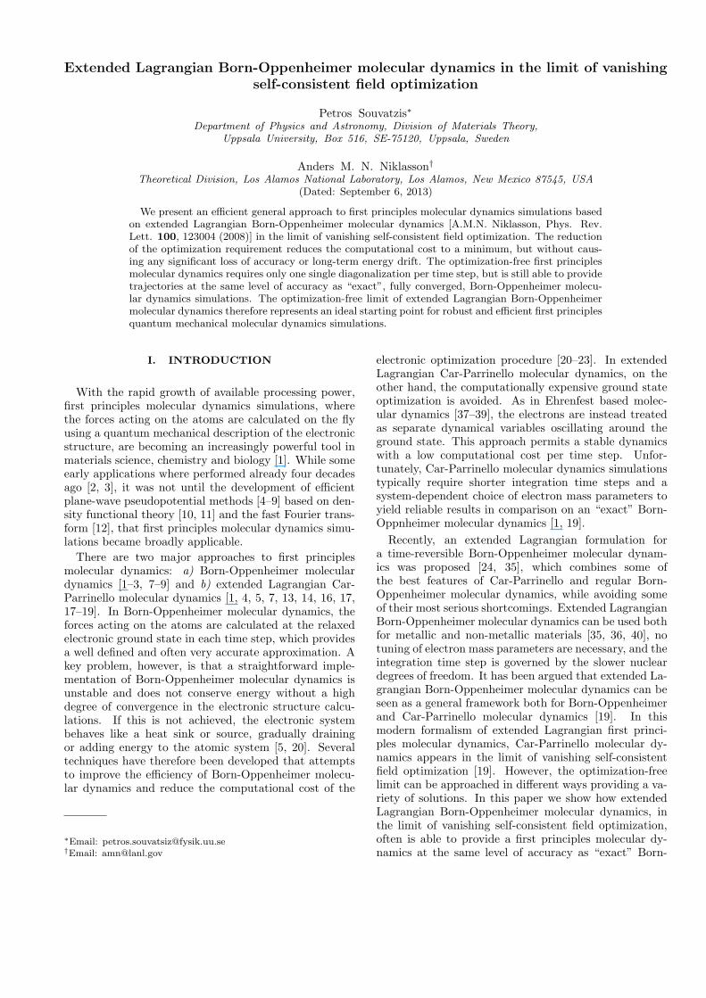
Figure 1 shows the behavior of the total energy, Eq.(5), for the simulation of a single water molecule usinga STO-3G basis set in (a) and a 6-31G∗∗ basis set in(b). The water structure was perturbed from equilib-rium with zero starting velocities as initial boundary con-dition. Regular Born-Oppenheimer molecular dynamics,where the density matrix from the previous time step wasused as the initial guess to the iterative ground-state op-timization, exhibits an unphysical systematic drift in thetotal energy because of the broken time-reversal symme-try [20, 24]. This drift is avoided in the “exact” fully op-timized extended Lagrangian Born-Oppenheimer molec-ular dynamics (XL-BOMD), Eq. (2), which is very closeto the results from the optimization-free fast first princi-ples QMMD (red circles), Eq. (6-7), as seen in the insets.In the lower panel (b) the deviation is slightly larger.However, any deviations between the optimization-freeand the fully optimized Born-Oppenheimer molecular dy-namics simulations are small compared to the local trun-cation error, i.e. the amplitude of the total energy fluc-tuations that are caused by the finite size of the integra-tion time step ∆t = 10 a. u. As in classical moleculardynamics, the dominating integration error is thus deter-mined by our choice of integration scheme and the sizeof the time step. Figure 2 demonstrates the long-termstability of our first principles fast-QMMD, which shows

4

FIG. 1: Total energy fluctuations for water using “exact”(5 SCF/step) Born-Oppenheimer molecular dynamics (XL-BOMD), Eq. (2), and the first principles fast-QMMD, i.e.XL-BOMD in the limit n→ 0, Eq. (6-7), in comparison to reg-ular Born-Oppenheimer molecular dynamics (BOMD), wherethe density matrix form the previous time step is used as theinitial guess to the SCF optimization with the energy con-verged to < 0.01 µHartree. In (a) a STO-3G basis set wasused, in the inset E0 = -74.949 au. In (b) a 6-31G∗∗ basis setwas used, in the inset E0 = -76.0058 au

0 20 40 60 80 100 120t [ps]

-0.1

-0.05

0

0.05

0.1

0.15

0.2

E -

E0 [

10-3

a.u

.]

XL-BOMDfast-QMMD

H2O (HF/STO-3G)

∆t = 10 a.u., T ~ 450 K

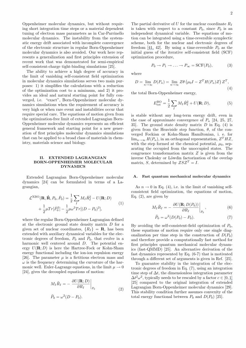
FIG. 2: Total energy fluctuations for a 130 ps simulation, us-ing “exact” (5 SCF/step) Born-Oppenheimer molecular dy-namics (XL-BOMD), Eq. (2), and the fast-QMMD, Eq. (6-7).Here E0 = -74.953 a.u.

0 1 2 3 4 5Time (ps)

-0.2

-0.1

0

0.1

0.2

0.3

0.4

E -

E0 [

10-3

a.u

.] XL-BOMDfast-QMMD

0 0.1 0.2Time (ps)

200

300

400

T [

K]

(H2O)

10

(HF/STO-3G)

∆t = 10 a.u.

E0 = -749.774 a.u.

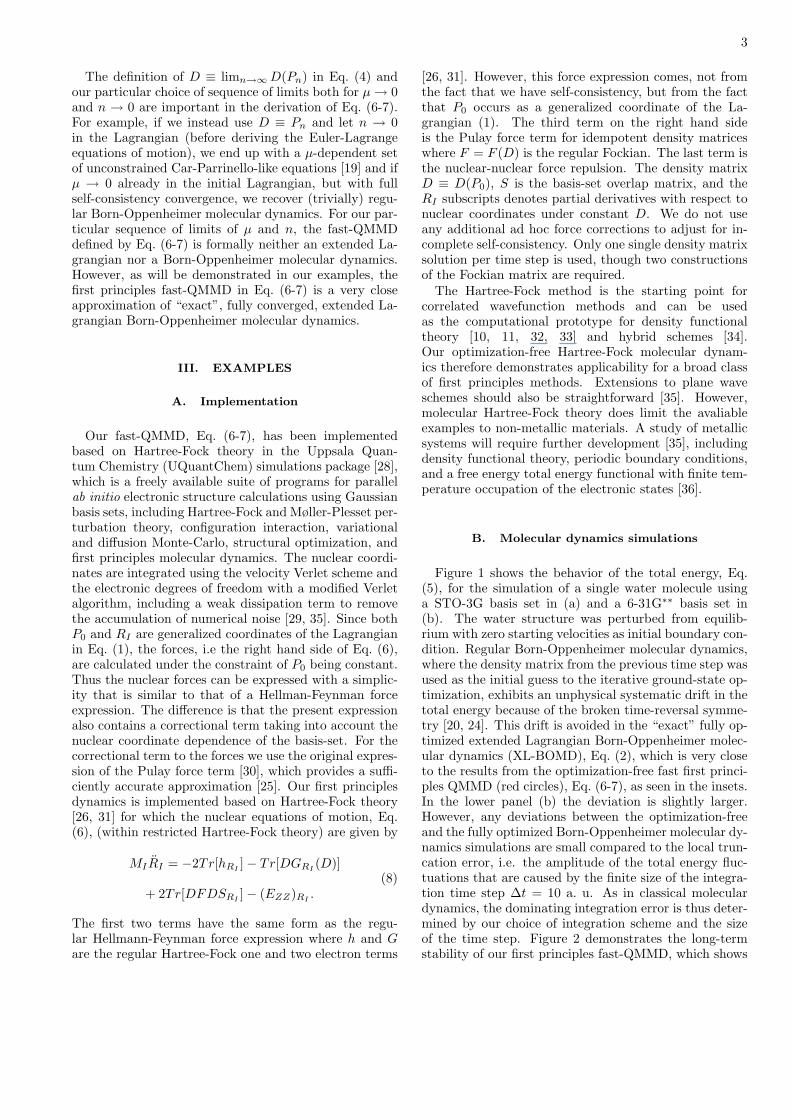
FIG. 3: Total energy fluctuations for a 5 ps simulation ofa small cluster containing 10 water molecules, using “exact”(5 SCF/step) Born-Oppenheimer molecular dynamics (XL-BOMD), Eq. (2), and the fast-QMMD, Eq. (6-7). Here E0 =-749.774 a.u. The inset shows the temperature fluctuationsfor the first 200 fs of simulation.

0.2

0.205

0.21

0.215E

-E0 [

mH

a]

C2H

6 (HF/6-31G**)

∆t = 5 a.u., T~190 K

∆t = 10 a.u., T ~ 190 K

XL-BOMDfast-QMMD

0 0.25 0.5 0.75 1 1.25 1.5t [ps]

0.15

0.16

0.17

0.18

0.190.2

0.21

0.22

E-E

0 [m

Ha]

C2H

6 (HF/6-31G**)

(a)

(b)

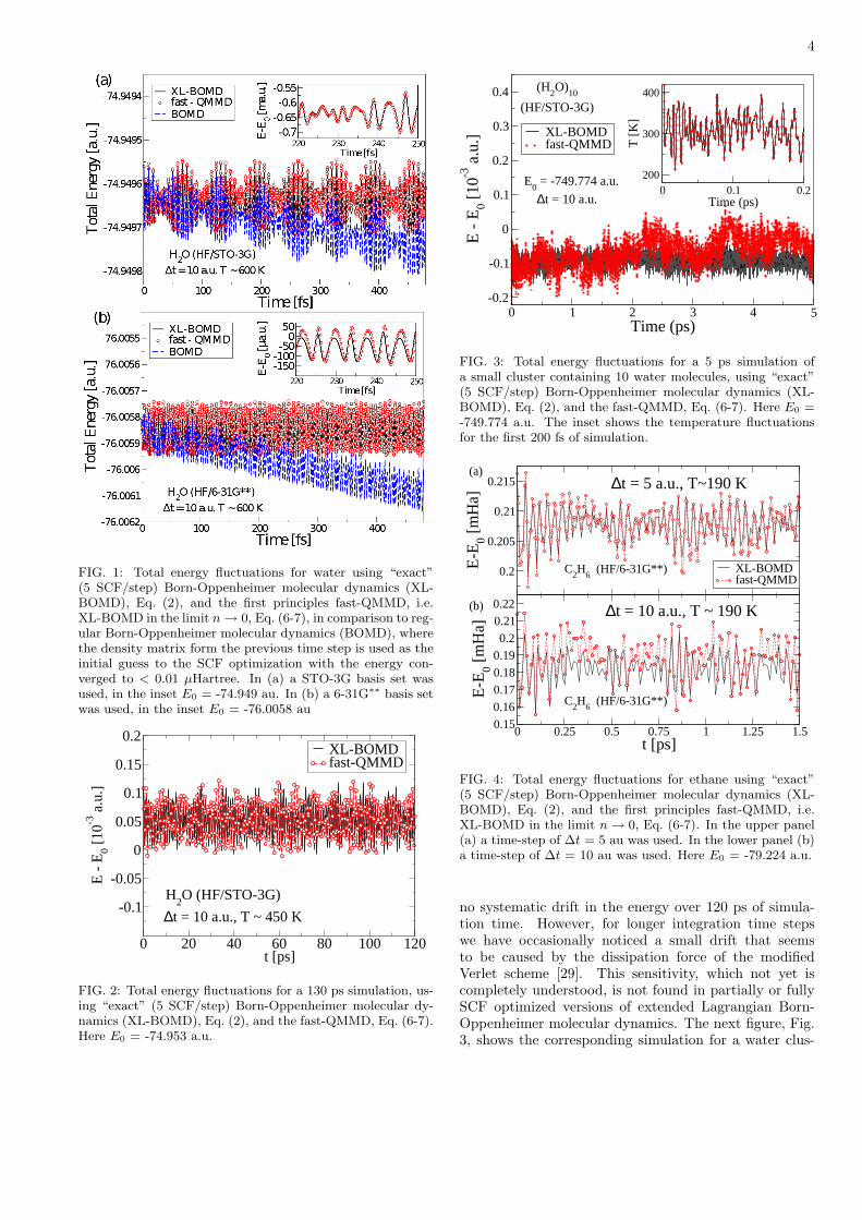
FIG. 4: Total energy fluctuations for ethane using “exact”(5 SCF/step) Born-Oppenheimer molecular dynamics (XL-BOMD), Eq. (2), and the first principles fast-QMMD, i.e.XL-BOMD in the limit n→ 0, Eq. (6-7). In the upper panel(a) a time-step of ∆t = 5 au was used. In the lower panel (b)a time-step of ∆t = 10 au was used. Here E0 = -79.224 a.u.

no systematic drift in the energy over 120 ps of simula-tion time. However, for longer integration time stepswe have occasionally noticed a small drift that seemsto be caused by the dissipation force of the modifiedVerlet scheme [29]. This sensitivity, which not yet iscompletely understood, is not found in partially or fullySCF optimized versions of extended Lagrangian Born-Oppenheimer molecular dynamics. The next figure, Fig.3, shows the corresponding simulation for a water clus-

5

-1

-0.75-0.5

-0.25

00.250.5

E-E

0 [·10

-3 a

.u.] XL-BOMD

fast-QMMD

0 100 200 300 400 500Time [fs]

2.65

2.7

2.75

2.8

2.85

E-E

0 [·10

-3 a

.u.]

H2O (HF/cc-pVTZ)

CF4 (HF/STO-3G)

(a)

(b)∆t = 20 a.u., T ~ 510 K

∆t = 40 a.u., T ~ 390 K

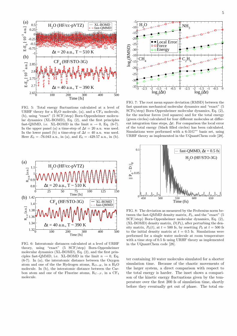
FIG. 5: Total energy fluctuations calculated at a level ofURHF theory for a H2O molecule, (a), and a CF4 molecule,(b), using “exact” (5 SCF/step) Born-Oppenheimer molecu-lar dynamics (XL-BOMD), Eq. (2), and the first principlesfast-QMMD, i.e. XL-BOMD in the limit n → 0, Eq. (6-7).In the upper panel (a) a time-step of ∆t = 20 a.u. was used.In the lower panel (b) a time-step of ∆t = 40 a.u. was used.Here E0 = -76.043 a.u., in (a), and E0 = -429.57 a.u., in (b).

0 25 50 75 100 125 150Time [fs]

0.8

0.9

1

1.1

RO

-H [

a.u.

]

XL-BOMDfast-QMMD

0 100 200 300 400 500Time [fs]

1.32

1.34

1.36

1.38

1.4

1.42

RC

-F [

a.u.

]

H2O (HF/cc-pVTZ)

CF4 (HF/STO-3G)

(a)

(b)

∆t = 20 a.u., T ~ 510 K

∆t = 40 a.u., T ~ 390 K

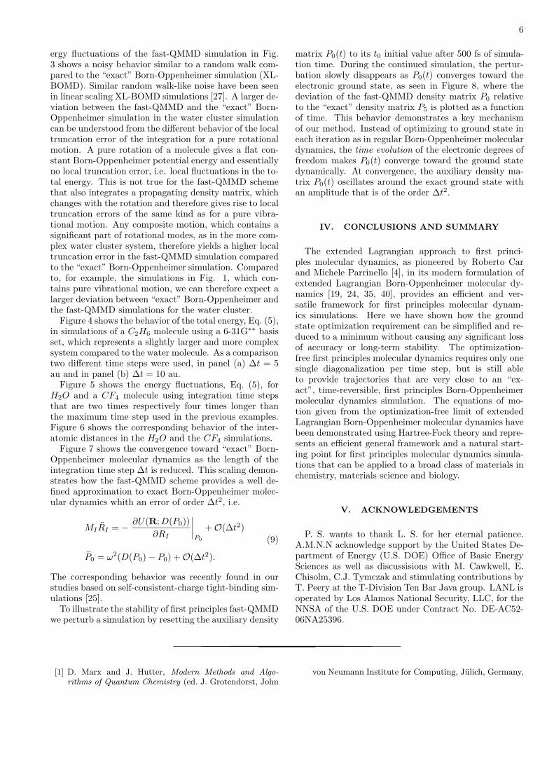
FIG. 6: Interatomic distances calculated at a level of URHFtheory, using “exact” (5 SCF/step) Born-Oppenheimermolecular dynamics (XL-BOMD), Eq. (2), and the first prin-ciples fast-QMMD, i.e. XL-BOMD in the limit n → 0, Eq.(6-7). In (a), the interatomic distance between the Oxygenatom and one of the the Hydrogen atoms, RO−H , in a H2Omolecule. In (b), the interatomic distance between the Car-bon atom and one of the Fluorine atoms, RC−F , in a CF4

molecule.

-30

-25

-20

-15

-10

-5

log 2(R

MSD

)

H2O

Local ErrorForceEnergy

NH3

-3 -2.5 -2 -1.5 -1 -0.5 0log

2(∆t)

-35

-30

-25

-20

-15

-10CH

4

-2.5 -2 -1.5 -1 -0.5 0log

2(∆t)

C2H

6

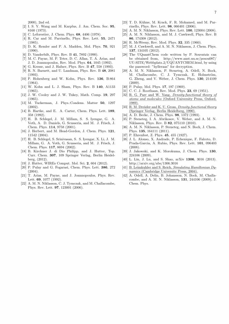
FIG. 7: The root mean square deviation (RMSD) between thefast quantum mechanical molecular dynamics and “exact” (5SCFs/step) Born-Oppenheimer molecular dynamics, Eq. (2),for the nuclear forces (red squares) and for the total energy(green circles) calculated for four different molecules at differ-ent integration time steps, ∆t. For comparison the local errorof the total energy (black filled circles) has been calculated.Simulations were performed with a 6-31G∗∗ basis set, usingURHF theory as implemented in the UQuantChem code [28].

450 500 550 600 650Time (fs)

0

0.05

0.1

|| P 0 -

D ||

F

fast-QMMD, ∆t = 0.5 fs

H2O (HF/STO-3G)

FIG. 8: The deviation as measured by the Frobenius norm be-tween the fast-QMMD density matrix, P0, and the ”exact” (5SCF/step) Born-Oppenheimer molecular dynamics, Eq. (2),(XL-BOMD) density matrix, D(P5), after perturbing the den-sity matrix, P0(t), at t = 500 fs, by resetting P0 at t = 500 fsto the initial density matrix at t = 0.5 fs. Simulations wereperformed for a single water molecule at room temperaturewith a time step of 0.5 fs using URHF theory as implementedin the UQuantChem code [28].

ter containing 10 water molecules simulated for a shortersimulation time. Because of the chaotic movements ofthe larger system, a direct comparison with respect tothe total energy is harder. The inset shows a compari-son of the kinetic energy fluctuations given by the tem-perature over the first 200 fs of simulation time, shortlybefore they eventually get out of phase. The total en-

6

ergy fluctuations of the fast-QMMD simulation in Fig.3 shows a noisy behavior similar to a random walk com-pared to the “exact” Born-Oppenheimer simulation (XL-BOMD). Similar random walk-like noise have been seenin linear scaling XL-BOMD simulations [27]. A larger de-viation between the fast-QMMD and the “exact” Born-Oppenheimer simulation in the water cluster simulationcan be understood from the different behavior of the localtruncation error of the integration for a pure rotationalmotion. A pure rotation of a molecule gives a flat con-stant Born-Oppenheimer potential energy and essentiallyno local truncation error, i.e. local fluctuations in the to-tal energy. This is not true for the fast-QMMD schemethat also integrates a propagating density matrix, whichchanges with the rotation and therefore gives rise to localtruncation errors of the same kind as for a pure vibra-tional motion. Any composite motion, which contains asignificant part of rotational modes, as in the more com-plex water cluster system, therefore yields a higher localtruncation error in the fast-QMMD simulation comparedto the “exact” Born-Oppenheimer simulation. Comparedto, for example, the simulations in Fig. 1, which con-tains pure vibrational motion, we can therefore expect alarger deviation between “exact” Born-Oppenheimer andthe fast-QMMD simulations for the water cluster.

Figure 4 shows the behavior of the total energy, Eq. (5),in simulations of a C2H6 molecule using a 6-31G∗∗ basisset, which represents a slightly larger and more complexsystem compared to the water molecule. As a comparisontwo different time steps were used, in panel (a) ∆t = 5au and in panel (b) ∆t = 10 au.

Figure 5 shows the energy fluctuations, Eq. (5), forH2O and a CF4 molecule using integration time stepsthat are two times respectively four times longer thanthe maximum time step used in the previous examples.Figure 6 shows the corresponding behavior of the inter-atomic distances in the H2O and the CF4 simulations.

Figure 7 shows the convergence toward “exact” Born-Oppenheimer molecular dynamics as the length of theintegration time step ∆t is reduced. This scaling demon-strates how the fast-QMMD scheme provides a well de-fined approximation to exact Born-Oppenheimer molec-ular dynamics whith an error of order ∆t2, i.e.

MIRI = − ∂U(R;D(P0))∂RI

∣∣∣∣P0

+O(∆t2)

P0 = ω2(D(P0)− P0) +O(∆t2).

(9)

The corresponding behavior was recently found in ourstudies based on self-consistent-charge tight-binding sim-ulations [25].

To illustrate the stability of first principles fast-QMMDwe perturb a simulation by resetting the auxiliary density

matrix P0(t) to its t0 initial value after 500 fs of simula-tion time. During the continued simulation, the pertur-bation slowly disappears as P0(t) converges toward theelectronic ground state, as seen in Figure 8, where thedeviation of the fast-QMMD density matrix P0 relativeto the “exact” density matrix P5 is plotted as a functionof time. This behavior demonstrates a key mechanismof our method. Instead of optimizing to ground state ineach iteration as in regular Born-Oppenheimer moleculardynamics, the time evolution of the electronic degrees offreedom makes P0(t) converge toward the ground statedynamically. At convergence, the auxiliary density ma-trix P0(t) oscillates around the exact ground state withan amplitude that is of the order ∆t2.

IV. CONCLUSIONS AND SUMMARY

The extended Lagrangian approach to first princi-ples molecular dynamics, as pioneered by Roberto Carand Michele Parrinello [4], in its modern formulation ofextended Lagrangian Born-Oppenheimer molecular dy-namics [19, 24, 35, 40], provides an efficient and ver-satile framework for first principles molecular dynam-ics simulations. Here we have shown how the groundstate optimization requirement can be simplified and re-duced to a minimum without causing any significant lossof accuracy or long-term stability. The optimization-free first principles molecular dynamics requires only onesingle diagonalization per time step, but is still ableto provide trajectories that are very close to an “ex-act”, time-reversible, first principles Born-Oppenheimermolecular dynamics simulation. The equations of mo-tion given from the optimization-free limit of extendedLagrangian Born-Oppenheimer molecular dynamics havebeen demonstrated using Hartree-Fock theory and repre-sents an efficient general framework and a natural start-ing point for first principles molecular dynamics simula-tions that can be applied to a broad class of materials inchemistry, materials science and biology.

V. ACKNOWLEDGEMENTS

P. S. wants to thank L. S. for her eternal patience.A.M.N.N acknowledge support by the United States De-partment of Energy (U.S. DOE) Office of Basic EnergySciences as well as discussisions with M. Cawkwell, E.Chisolm, C.J. Tymczak and stimulating contributions byT. Peery at the T-Division Ten Bar Java group. LANL isoperated by Los Alamos National Security, LLC, for theNNSA of the U.S. DOE under Contract No. DE-AC52-06NA25396.

[1] D. Marx and J. Hutter, Modern Methods and Algo-rithms of Quantum Chemistry (ed. J. Grotendorst, John

von Neumann Institute for Computing, Julich, Germany,

7

2000), 2nd ed.[2] I. S. Y. Wang and M. Karplus, J. Am. Chem. Soc. 95,

8160 (1973).[3] C. Leforestier, J. Chem. Phys. 68, 4406 (1978).[4] R. Car and M. Parrinello, Phys. Rev. Lett. 55, 2471

(1985).[5] D. K. Remler and P. A. Madden, Mol. Phys. 70, 921

(1990).[6] D. Vanderbilt, Phys. Rev. B 41, 7892 (1990).[7] M. C. Payne, M. P. Teter, D. C. Allan, T. A. Arias, and

J. D. Joannopoulos, Rev. Mod. Phys. 64, 1045 (1992).[8] G. Kresse, and J. Hafner, Phys. Rev. B 47, 558 (1993).[9] R. N. Barnett, and U. Landman, Phys. Rev. B 48, 2081

(1993).[10] P. Hohenberg and W. Kohn, Phys. Rev. 136, B:864

(1964).[11] W. Kohn and L. J. Sham, Phys. Rev. B 140, A1133

(1965).[12] J. W. Cooley and J. W. Tukey, Math. Comp. 19, 297

(1965).[13] M. Tuckerman, J. Phys.:Condens. Matter 50, 1297

(2002).[14] B. Hartke, and E. A. Carter, Chem. Phys. Lett. 189,

358 (1992).[17] H. B. Schlegel, J. M. Millam, S. S. Iyengar, G. A.

Voth, A. D. Daniels, G. Scusseria, and M. J. Frisch, J.Chem. Phys. 114, 9758 (2001).

[16] J. Herbert, and M. Head-Gordon, J. Chem. Phys. 121,11542 (2004).

[17] H. B. Schlegel, S. Srinivasan, S. S. Iyengar, X. Li, J. M.Millam, G. A. Voth, G. Scusseria, and M. J. Frisch, J.Chem. Phys. 117, 8694 (2002).

[18] B. Kirchner J. di Dio Philipp, and J. Hutter, Top.Curr. Chem. 307, 109 Springer Verlag, Berlin Heidel-berg, (2012).

[19] J. Hutter, WIREs Comput. Mol. Sci. 2, 604 (2012).[20] P. Pulay and G. Fogarasi, Chem. Phys. Lett. 386, 272

(2004).[21] T. Arias, M. Payne, and J. Joannopoulos, Phys. Rev.

Lett. 69, 1077 (1992).[22] A. M. N. Niklasson, C. J. Tymczak, and M. Challacombe,

Phys. Rev. Lett. 97, 123001 (2006).

[23] T. D. Kuhne, M. Krack, F. R. Mohamed, and M. Par-rinello, Phys. Rev. Lett. 98, 066401 (2006).

[24] A. M. N. Niklasson, Phys. Rev. Lett. 100, 123004 (2008).[25] A. M. N. Niklasson, and M. J. Cawkwell, Phys. Rev. B

86, 174308 (2012).[26] R. McWeeny, Rev. Mod. Phys. 32, 335 (1960).[27] M. J. Cawkwell, and A. M. N. Niklasson, J. Chem. Phys.

137, 134105 (2012).[28] The UQuantChem code written by P. Souvatzis can

be obtained from, http://www.anst.uu.se/pesou087/UU-SITE/Webbplats 2/UQUANTCHEM.html, by usingthe password: ”hylleraas” for decryption.

[29] A. M. N. Niklasson, P. Steneteg, A. Odell, N. Bock,M. Challacombe, C. J. Tymczak, E. Holmstrom,G. Zheng, and V. Weber, J. Chem. Phys. 130, 214109(2009).

[30] P. Pulay, Mol. Phys. 17, 197 (1969).[31] C. C. J. Roothaan, Rev. Mod. Phys. 23, 69 (1951).[32] R. G. Parr and W. Yang, Density-functional theory of

atoms and molecules (Oxford University Press, Oxford,1989).

[33] R. M. Dreizler and K. U. Gross, Density-functional theory(Springer Verlag, Berlin Heidelberg, 1990).

[34] A. D. Becke, J. Chem. Phys. 98, 1372 (1993).[35] P. Steneteg, I. A. Abrikosov, V. Weber, and A. M. N.

Niklasson, Phys. Rev. B 82, 075110 (2010).[36] A. M. N. Niklasson, P. Steneteg, and N. Bock, J. Chem.

Phys. 135, 164111 (2011).[37] P. Ehrenfest, Z. Phys. 45, 455 (1927).[38] J. L. Alonso, X. Andrade, P. Echenique, F. Falceto, D.

Prada-Garcia, A. Rubio, Phys. Rev. Lett. 101, 096403(2008).

[39] J. Jakowski, and K. Morokuma, J. Chem. Phys. 130,224106 (2009).

[40] L. Lin, J. Lu, and S. Shao, arXiv 1306, 3016 (2013).http://arxiv.org/abs/1306.3016

[41] B. Leimkuhler and S. Reich, Simulating Hamiltonian Dy-namics (Cambridge University Press, 2004).

[42] A. Odell, A. Delin, B. Johansson, N. Bock, M. Challa-combe, and A. M. N. Niklasson, 131, 244106 (2009), J.Chem. Phys.