EXPORT RESPONSE TO THE REDUCTION OF ANTI … · The continual depreciation of the nominal exchange rate, ... liberalisation periods. As mentioned before, Bangladesh initiated the

EXPORT RESPONSE TO THE REDUCTION OF ANTI-EXPORT BIAS: EMPIRICS FROM BANGLADESH

Mohammad A. Hossain and

Neil Dias Karunaratne School of Economics

The University of Queensland Brisbane Qld 4072

January 2002

Discussion Paper No. 303

ISSN 1033-4661

© Hossein and Karunaratne 2001

This discussion paper representations work-in-progress and should not be quoted or reproduced in whole or in part without the written consent of the author.

EXPORT RESPONSE TO THE REDUCTION OF ANTI-EXPORT BIAS: EMPIRICS FROM BANGLADESH

Mohammad A Hossain and Neil Dias Karunaratne

Abstract The paper assesses the relationship between export growth of Bangladesh and trade liberalisation, the latter being proxied by the reduction of anti-export bias. In the empirical analysis, separate supply equations for total exports, (total) manufacturing exports, and textiles and readymade garment exports have been undertaken using quarterly time series data. The empirical results, based on vector error correction modelling (VECM), show that trade liberalisation has both long run and contemporaneous effects on total exports, manufacturing exports, and textiles and readymade garment exports supply. Besides, domestic price, export price, anti-export bias reduction, the degree of openness and production capacity all have either unidirectional or bi-directional causality between them. Key Words: anti-export bias reduction, cointegration, error correction modeling, general-to-specific modeling,

granger causality, trade liberalisation.

(JEL Code: C32, F13, F14.)

1

1. INTRODUCTION

The purpose of the paper is to empirically examine the relationship between expansion of exports

and trade liberalisation as proxied by the trade policy bias (TPB) or anti-export bias, in an

underdeveloped economy. The trade policy bias (TPB) or anti-export bias is defined as the ratio

of the real effective exchange rate applied to exports (REERX) to the real effective exchange rate

applied to imports (REERM)1 REERX and REERM are the weighted indices of the nominal

bilateral exchange rates for exports and imports respectively of Bangladesh's major trading

partners, adjusted for the changes in the domestic consumer prices relative to the partner

countries. The weights used are the 1995 export- and import shares respectively of 22 major

trading partners of Bangladesh.2 This is precisely the method advocated by Bahmani-Oskoooee

(1995) except that we calculate the one-dollar equivalent of Bangladesh taka instead of vice

versa and that we replace the official exchange rate by the nominal exchange rates for exports

and imports. As defined, an increase in REERX or REERM represents depreciation and, hence, an

increase TPB represents anti-export bias reduction

The rationale for the study stems from the contention that recent expansion of exports of the

developing countries in general, and that of the High Performance Asian Economies (HPAEs) in

particular, is the result of the implementation of export-oriented growth strategies in the 1970s

and the 1980s spearheaded by an increase in manufacturing exports. Manufacturing exports have

emerged as the new engine of the export-oriented growth for these countries replacing the total-

export engine [Reidel, 1993; Helleiner, 1994 and 1995; Weiss, 1992; Thomas and Nash, 1991;

1 The definition follows from Bhagwati (1978). A value of REERX/REERM = 1 is described as a pro-export bias strategy. REERX/REERM >1 represents an ultra pro-export bias regime. while REERX/REERM < 1 indicates an anti-export bias policy. 2 The countries considered here include: Australia, Belgium, Canada, Denmark, France, Germany, Hong Kong, India, Indonesia, Italy, Japan, Korea, Malaysia, the Netherlands, Norway, Pakistan, Singapore, Spain, Sweden, Switzerland, UK and USA which accounted for 87% of Bangladesh's exports and 68% of imports in 1995. The two

2

Joshi and little, 1996; and Krueger, 1997]. These two propositions constitute the controversial de

novo hypothesis. The anti-export bias reduction hypothesis formed in this study postulates that a

typical developing country experimented with an import-substituting industrialising (ISI)

strategy and used it as a stepping stone to embark on export-led growth, whilst the de novo

hypothesis denies the stepping stone effect of the ISI and asserts that export oriented

manufacturing industries started a new engine of growth. Several studies (Little et al. (1970),

Balassa (1971 and 1982), Bhagwati (1978), Krueger (1978), Michaely et al. (1991) and

Athukorala (1998)) suggest that there is a positive relationship between trade liberalisation and

export expansion. On the other hand, studies by UNCTAD (1989), Agosin (1991), Shafaeuddin

(1994), Clarke and Kirkpatrick (1992) find that trade liberalisation retarded export expansion.

In this paper we attempt to shed light on this controversial issue by using Bangladesh as a case

study. Bangladesh inherited an inward-oriented policy regime at its independence in 1971, which

it continued until the early part of the 1980's. The country has, in effect, been pursuing an

outward-looking strategy since 1982, when it initiated the structural adjustment programmes at

the behest of the World Bank. The three key areas of the Bangladesh economy, trade, financial

and fiscal, have undergone various types of changes although the trade sector reforms stand out

to be the most significant [World Bank 1996:V]. It is, therefore, worthwhile to examine how

exports responded to these stimuli. Bangladesh experience provides insights on how trade

liberalisation promoted exports [Rahman, 1992 and 1995; Bayes, et al., 1995; Hossain et al.,

1997; Ahmed, 2000]. However, barring Ahmed (2000), these studies are flawed as they are

subject to spurious statistical inferences because of the failure to test for stochastic trends (unit

roots) in the time series data. Ahmed (2000) presents a more rigorous treatment of the issue.

However, the study suffers from two serious drawbacks. First, it uses the ratio of unit export

notable omissions are China and Thailand especially from the point of view of imports. These two countries could not be included due to lack of consistent data set for the exchange rates and the consumer price indices.

3

price of Bangladesh to that of the industrialised countries as the relative price of Bangladesh's

exports. From the exporting country's point of view, this makes sense only if interpreted as an

index of international competitiveness. Even in that case, the unit price index of the

underdeveloped countries would have been more appropriate since these are the countries

Bangladesh competes with in the world export market. Second, the study identifies 1991 as the

breakpoint of the policy regime. But available documents and studies show that the

rationalisation of the trade regime started in 1982 and was further consolidated in 1985-86 before

being overhauled by a third intensive phase beginning in 1991 [Shand and Alauddin, 1996;

Salim, 1999]. The present study overcomes the drawbacks mentioned above by choosing more

appropriate variables. The study also explicitly defines and calculates a trade policy bias index

(TPB) and uses it as a separate argument rather than using REERX to proxy for it. Indeed, the

construction of the anti-export bias index itself constitutes part of the contribution of this study.

Also considered in this study is the degree of openness (DOP) defined as the ratio of total trade

(exports + imports) to gross domestic product (GDP) to represent the intensity of trade and the

importance of the external trade sector. DOP also captures the extent of import liberalisation,

which might have a 'spill-over' effect on exports. Finally, the analysis is extended to examine the

performance of manufacturing exports, and textile and readymade garment exports and thereby

to address the main thrust of the de novo hypothesis. Indeed, as can be seen from Table 3.1

(Section 3), manufacturing, and textile and readymade garment exports grew at rates much

faster than total exports. The analysis is done by estimating three separate supply equations for

total exports, manufacturing exports, and textile and readymade garment exports by applying the

vector error correction modelling. It is intended that an analysis of the export performance at the

disaggregated levels should provide more effective policy implications. The rest of the paper is

organised as follows. Section 2 gives a brief overview of the Bangladesh's exchange rate regime.

Section 3 presents the trends in exports. Section 4 sets out the analytical framework. Section 5

4

describes the data and their time series properties. Section 6 and 7 report the estimated results.

And finally, Section 8 presents the conclusion.

2. A BRIEF OVERVIEW OF BANGLADESH'S EXCHANGE RATE REGIME

Since anti-export bias reduction is defined in terms of the exchange rates, it is worthwhile to

provide a brief preview of the Bangladesh's exchange rate regime. Bangladesh had a pegged

exchange rate system and in August 1979 it was made a managed float. In 1993 the national

currency, taka, was floated and made convertible on the current account. The current account

convertibility is considered as a precondition to further liberalisation of the exchange rate

regime. The continual depreciation of the nominal exchange rate, especially since 1985 provided

an extra impetus on the speed of consolidation of the foreign exchange regime. Since 1974 the

various measures of real exchange rates, defined in terms of domestic currency per US dollar

show secular increase implying the depreciation of the domestic currency, taka. For example, in

1976 the real effective exchange rate for exports (REERX) was 25.31 taka/US dollar. In 1986 it

was 32.59 taka/US dollar and in 1998 the rate was 38.52/US dollar. The real effective exchange

rate for imports (REERM) also shows an upward tendency over time, although the rate of

increase is rather slow. The corresponding figures for REERM for the years mentioned above are

37.97, 39.92 and 39.50 respectively. That very aptly explains why the trade policy bias index

(TPB) registers an upward movement meaning a reduction in anti-export bias over time. The

TPB rose from 0.67 in 1976 to 0.82 in 1986 to 0.98 in 1998. The quarterly data might capture the

dynamics of the exchange rate policy more effectively. We, therefore, present the quarterly data

(index: 1995=100) on REERX, REERM and TPB in Figure 2.1.

5

Figure 2.1: Plots of REERX, REERM and TPB (Index: 1995=100)

3. TRENDS AND CHANGING PATTERNS OF EXPORTS OF BANGLADESH

The depreciation of the domestic currency as discussed in the previous section indicates a

reduction in the anti-export bias. This was proved conducive to the growth of exports. In fact,

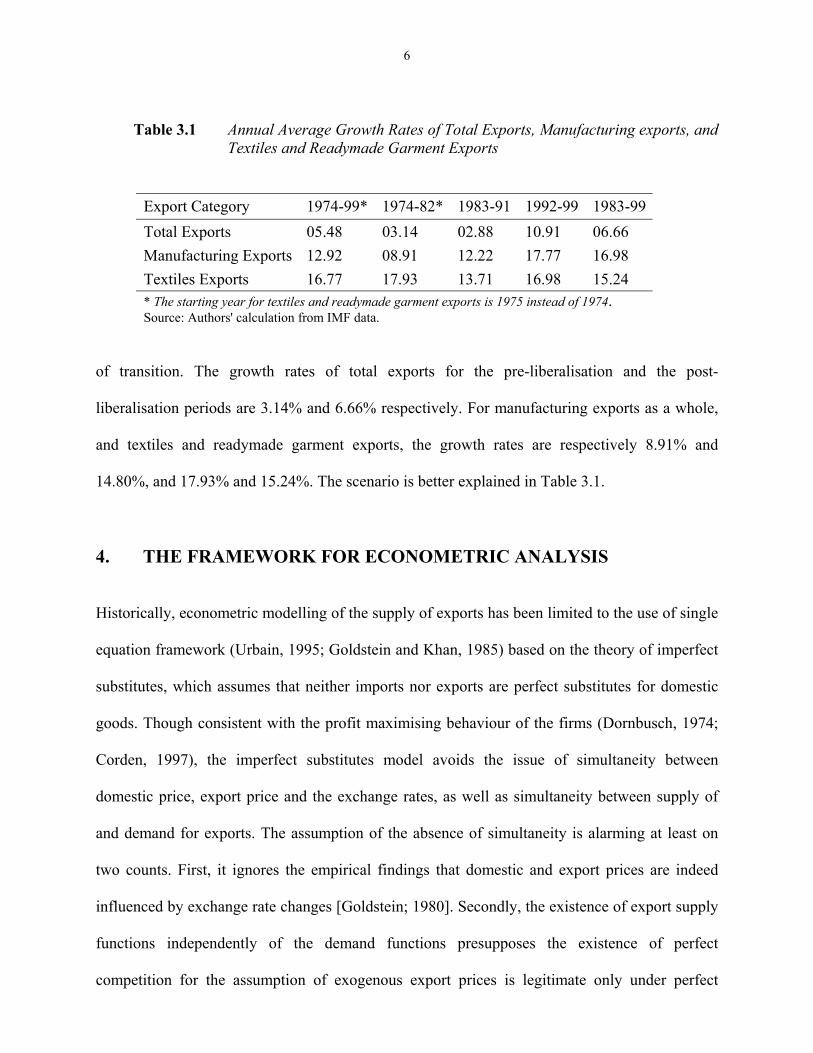
real total exports increased by an average annual rate of 5.48% over the study period 1974-1999.

Real manufacturing exports grew at an average annual rate of 12.92% during the same period

while real textiles and readymade garment exports grew at an average annual rate of 16.78%

during 1975-1999. However, the growth rates differ across the pre-liberalisation and the post-

liberalisation periods. As mentioned before, Bangladesh initiated the transition towards outward-

orientation in 1982 and took a gradualist approach to remove the controls on the external sector.

The 1982 efforts were followed by measures in 1985-86 and 1991. Therefore, we interpret the

period until 1982 as the pre-liberalisation era and the period from 1982 onwards as the post-

liberalisation era of which, period 1983 through 1991 can be described as the period

6

Table 3.1 Annual Average Growth Rates of Total Exports, Manufacturing exports, and

Textiles and Readymade Garment Exports

Export Category 1974-99* 1974-82* 1983-91 1992-99 1983-99 Total Exports 05.48 03.14 02.88 10.91 06.66 Manufacturing Exports 12.92 08.91 12.22 17.77 16.98 Textiles Exports 16.77 17.93 13.71 16.98 15.24 * The starting year for textiles and readymade garment exports is 1975 instead of 1974. Source: Authors' calculation from IMF data.

of transition. The growth rates of total exports for the pre-liberalisation and the post-

liberalisation periods are 3.14% and 6.66% respectively. For manufacturing exports as a whole,

and textiles and readymade garment exports, the growth rates are respectively 8.91% and

14.80%, and 17.93% and 15.24%. The scenario is better explained in Table 3.1.

4. THE FRAMEWORK FOR ECONOMETRIC ANALYSIS

Historically, econometric modelling of the supply of exports has been limited to the use of single

equation framework (Urbain, 1995; Goldstein and Khan, 1985) based on the theory of imperfect

substitutes, which assumes that neither imports nor exports are perfect substitutes for domestic

goods. Though consistent with the profit maximising behaviour of the firms (Dornbusch, 1974;

Corden, 1997), the imperfect substitutes model avoids the issue of simultaneity between

domestic price, export price and the exchange rates, as well as simultaneity between supply of

and demand for exports. The assumption of the absence of simultaneity is alarming at least on

two counts. First, it ignores the empirical findings that domestic and export prices are indeed

influenced by exchange rate changes [Goldstein; 1980]. Secondly, the existence of export supply

functions independently of the demand functions presupposes the existence of perfect

competition for the assumption of exogenous export prices is legitimate only under perfect

7

competition [Goldstein and Khan, 1985]. The fundamental logic behind considering the demand

side alongside the supply side in the imperfect substitutes models, as Orcutt (1950) points out, is

to spell out that the relationship between quantities and prices is simultaneous, at least in theory.

The issue of simultaneity is especially important when it comes to assessing the impact of

alternative trade regimes on trade flows [Urbain, 1995]. In the empirical framework used to test

rival hypotheses in this paper, we apply the Vector Error Correction (VEC) modelling. This

methodology overcomes the limitations of the past empirics

4.1 Explanation of and Rationale for the Choice of the Non-Export Variables

In implementing the vector error correction modelling (VECM), the following variables have

been considered:

TXt = real total exports;

MXt = real (total) manufacturing exports;

TXXt=real textile exports including readymade garments;

PXt = price of exports;

PDt = domestic price

TPBt = REERX / REERM trade policy bias or anti-export bias;

PCt = production capacity;

DOPt = degree of openness;

t = time subscript.

The domestic price here is represented by the domestic wholesale price index. The inclusion of

the domestic price in the model serves two purposes. First, given export price, the profitability of

producing and selling exports decreases as factor costs increase in the export industries. Since

factor costs are likely to be correlated with domestic price, the latter acts as a proxy for the

8

former. Secondly, domestic price includes both the prices of tradables sold at home as well as the

nontradables. Thus domestic price captures supply substitution between the home and export

market for a given tradable good as well as all tradables and nontradables. The inclusion of the

price of export captures the internal profitability of producing and selling export goods. The

trade policy bias (TPB) indicates the degree of export-orientation. The production capacity, PCt,

is represented by the incremental fixed capital formation or investment in the economy as a

whole. While PXt, PDt and TPBt are expected to influence exports as a result of the movement

along the production possibility curve, PCt captures the shifts in the production possibility curve

over time. The latter is alone sufficient to bring about changes in exports in the absence of any

changes in PXt, PDt or TPBt. Defined as the trade-GDP ratio, DOPt measures the importance of

the foreign trade sector and, to an extent, import liberalisation. All the explanatory variables,

except PDt, are expected to have positive coefficients. All the variables including the prices are

expressed in domestic currency.

4.2 The Empirical Technique

As mentioned before, the study applies cointegration and vector error correction modelling in

order to estimate the export supply equations. The literature on time series econometrics suggests

a number of alternatives to deal with non-stationarity in the data, of which the Box-Jenkins

ARIMA approach (Box and Jenkins, 1970), the Vector Autoregression (Sims, 1980),

Cointegration and Error Correction Model (Engle and Granger, 1987) and the Maximum

Likelihood in a Fully Specified Error Correction model (MLECM) (Johansen, 1988 and

Johansen and Juselius, 1992) are the examples. For quite sometime, the Engle-Granger

procedure had been the 'state-of-the-art' methodology in testing causality in economic models

where all the variables are treated as endogenous. However, due to better statistical properties,

9

the Johansen-Juselius MLECM got wider acceptance in empirical applications. 3 One advantage

with the latter is that, unlike the former, it produces identical error correction term irrespective of

the choice of the variable to be normalised. In addition, the MLECM can explain Granger

causality, overcoming the problems of simultaneity bias. In order to specify the Vector Error

Correction Model in the Johansen-Juselius proper, we proceed as follows. Concentrating on total

export supply, the six-variable VAR model can be described as follows:

V = (TXt, PXt, PDt, TPBt, DOPt, PCt)′ (4.1.)4.

The corresponding unrestricted VAR model with the deterministic term can be specified as

Vt = A0 + A(L)Vt + εt (4.2)

where, A(L) = (aij(L)) is a 6 × 6 matrix of the polynomial and aij(L) = Σ aij,1L1, mij is the degree

of the polynomial. A0 = (a10 a20 a30 a30 a50 a60)′ is a constant, and εt is 6 × 1 vector of the

random errors. Assuming exactly one cointegrating vector to exist between the variables and that

the variables are stationary in the first differences, Model (4.1) can be rewritten as

∆

Vt = A0 + A(L) ∆Vt-1 + δ ECt-1 + µt (4.3)

where ECt denotes the error correction term. µt is a 6 × 1 vector of white noise errors, that is,

E(µt) = 0 and E(µt µ t-s) = σ for t = s and zero otherwise. Using the lower case letters to denote

3 For a comparative analysis of the alternative empirical techniques dealing with 'non-stationary data, see for example, Enders, 1995 and Maddala and Kim, 1998. Gonzalo (1994) contains a detailed discussion on the relative merit of the alternative methods suggested for cointegrated systems. Of Ordinary Least Squares (Engle and Granger, 1987), Non-Linear Least Squares (Stock, 1987), Principal Components (Stock and Watson, 1988) and MLECM (Johansen, 1988 and Johansen and Juselius, 1992), Gonzalo finds MLECM to capture the desirable elements in a cointegrated system. 4 The manufacturing export supply and the textiles and readymade garment supply models can be formed in a similar way in that TXt is replaced by MXt and TXXt respectively.

10

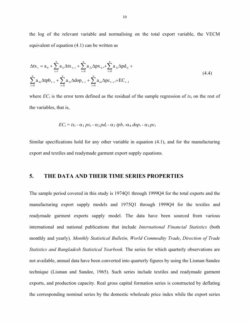
the log of the relevant variable and normalising on the total export variable, the VECM

equivalent of equation (4.1) can be written as

1tit

n

0ii6it

n

0ii5it

n

0ii4

ti

n

0ii3ti

n

0ii2it

n

1ii10t

EC,pcadopatpba

pda,pxatxaatx

−−=

−=

−=

==−

=

+∆+∆+∆

+∆+∆+∆+=∆

∑∑∑

∑∑∑ (4.4)

where ECt is the error term defined as the residual of the sample regression of txt on the rest of

the variables, that is,

ECt = txt - α1 pxt - α2 pdt - α3 tpbt -α4 dopt - α5 pct

Similar specifications hold for any other variable in equation (4.1), and for the manufacturing

export and textiles and readymade garment export supply equations.

5. THE DATA AND THEIR TIME SERIES PROPERTIES

The sample period covered in this study is 1974Q1 through 1999Q4 for the total exports and the

manufacturing export supply models and 1975Q1 through 1999Q4 for the textiles and

readymade garment exports supply model. The data have been sourced from various

international and national publications that include International Financial Statistics (both

monthly and yearly), Monthly Statistical Bulletin, World Commodity Trade, Direction of Trade

Statistics and Bangladesh Statistical Yearbook. The series for which quarterly observations are

not available, annual data have been converted into quarterly figures by using the Lisman-Sandee

technique (Lisman and Sandee, 1965). Such series include textiles and readymade garment

exports, and production capacity. Real gross capital formation series is constructed by deflating

the corresponding nominal series by the domestic wholesale price index while the export series

11

are converted into real figures by deflating them by the unit price index of exports of

Bangladesh. All the variables are expressed in domestic currency.

5.1 The Order of Integration of the Variables

In order to test for 'stationarity' or the order of integration of the time series, first the series have

been tested for the presence of structural breaks or jumps5 by using three pulse dummies, DP1,

DP2 and DP3, for the years 1982, 1986 and 1991 respectively6. The results are presented in Table

5.1. The ‘t’ values corresponding to the coefficients of the pulse dummy variables for each

series, suggest that there is no break in any of the sequences since none of the DPj coefficients

are statistically significant even at a 10% level of significance.

Table 5.1: 't' Values of the Coefficients of the Pulse Dummy Variables*

Series Sample Size 't'-DP1 't'-DP2 't'-DP3 txt 103 0.16 0.04 -0.02 mxt 103 -0.34 1.30 1.12 txxt 99 -0.19 1.42 0.38 pxt 103 1.24 -1.26 -0.24 pdt 103 -0.26 -0.41 -0.93 tpbt 103 0.79 0.11 -0.33 dopt 103 -0.65 0.19 0.37 pct 103 1.37 1.31 -0.38 • 't' values correspond to the equation: yt = yt-1 + ∈t + DP1 + DP2 + DP3 where DP1 =1 for 1982

and 0 otherwise, DP2= 1 for 1986 and 0 otherwise and DP3 = 1 for 1991 and 0 otherwise.

5 The presence of a break or jump have different implications for unit root testing and cointegration [Zivot and Andrews, 1992; Gregory and Hansen, 1996; Ben-David et al., 1997]. 6 Major policy reforms in the form of structural structural adjustments took place in Bangladesh in three phases in the years mentioned. Although some suggest that the location of a breakpoint is unknown, as Maddala and Kim (1998) point out, one may look for a breakpoint around a period when major policy shifts occurred.

12

Table 5.2: Summary Results of the Nested Hypothesis*

Series Sample Size tρ^

tx 102 3.40 mx 102 2.13 txx 97 2.05 px 102 3.02 pd 102 2.53 tpb 102 1.96 dop 102 1.88 pc 102 3.17

*A TSP can be distinguished from a DSP as follows: TSP: yt = α + δ t + ut DSP: yt = α + ρyt-1 + ut

where ut is stationary. The nested model can be written as yt = α + δt + ρyt-1 + et

where et is assumed to be white noise. If the null hypothesis of H0: ρ = 1 and δ = 0 is rejected on the basis of the sample regression, then yt is TSP; else it belongs to the DSP class. The t-values are to be compared with the critical 't'. The one-tailed 't' at 5% level of significance and for a sample of 100 is -3.45 (from Nelson and Plosser, 1982, p. 151).

The absence of a break or jump in the data series implies that the conventional unit root testing

procedure can be used to determine the order of integration of the variables. Applying the

Augmented Dickey-Fuller (ADF) and the Phillips-Perron (PP) unit root tests, we find all the

variables to be non-stationary in their levels. The test statistics are reported in Table 1 in the

Appendix. A non-stationary series can be made stationary by detrending or differencing

depending on whether the series contains a trend stationary process (TSP) or a difference

stationary process (DSP). To see if the variables are TSP or DSP, we carry out a Nelson-Plosser-

Bhargava type hypothesis testing that nests a TSP with a DSP [Nelson and Plosser, 1982;

Bhargava, 1986]. The results, summarized in Table 5.2, show that all of the variables considered

in this study fall into the DSP category.

13

The ADF and the PP tests on the first differences of the variables show that the hypothesis of

unit root can be rejected for all the variables considered. We, therefore, conclude that all the

level variables follow an I(1) process. The results are presented in Table 2 in the Appendix.

5.2 Test for Cointegration

Let us first consider the total export supply model. The relevant variable vector is: (txt, pxt, pdt,

tpbt, dopt, pct)′. To determine the order of the VAR, we begin with an arbitrary lag length of 12 in

the unrestricted VAR that includes three centered seasonal dummies besides the six variables.

While the Akaike Information criterion (AIC) suggests an order of the VAR of 4, the Schwarz

Bayesian Criterion (SBC) suggests an order of 2. Both the orders are supported by the Adjusted

Likelihood Ratio (LR) test. Since the SBC has superior large sample properties while the AIC

favours an overparameterised model in general, one is tempted to applying the SBC. However, in

a situation like this, one must look at the residual serial correlation as well as normality of the

individual equations in the unrestricted VAR [Pesaran and Pesaran, 1997]. Both the orders fail to

satisfy either or both the conditions for the equations for all six variables. As can be seen from

Figure 1 in the Appendix, the first differences of the variables show important outliers in the

years 1974, 1975, 1977, 1978, 1981, 1983, 1984, 1986 and 1994; the most common being 1975

that succeeded the 1974 famine. Using dummies for the outliers, and for the three phases of

microeconomic reforms in 1982, 1986 and 1991, d1, d2 and d3 respectively, we find a third order

VAR to satisfy the serial correlation and normality conditions of the individual equations in the

unrestricted VAR. We, therefore, choose a third order VAR for the total export model.

In order to examine the number of cointegrating vectors (CV) in the model, we compute the

maximum eigen value statistic (λmax) and the trace statistic (λtrace) according to the Johansen-

14

Juselius procedure. Both criteria indicate the existence of two cointegrating relationships

between the I(1) variables in the model. The results are presented in Table 5.3. The λmax test

rejects the null hypothesis of no cointegration (r = 0) against the alternative of one cointegrating

relationship (r = 1) since the test statistic of 46.77 is greater than the 95 percent quintile value of

36.27. The λmax test also rejects the null hypothesis of r ≤ 1 against the alternative hypothesis of r

= 2 at 5 percent level of significance. However, the λmax test cannot reject the null of r ≤ 2

against the alternative of r = 3. Similarly, λtrace test rejects the null hypotheses of r =0 and r ≤ 1

against the alternative hypotheses of r ≥ 1 and r ≥ 2 respectively but not r ≤ 2 against r ≥ 3. The

results lead to the conclusion that there are two cointegrating vectors in the total export supply

model.

It is not surprising that more than one cointegrating relationship exist among the variables. It

might be argued that in the long run, the relevant price to be considered is the price of exports,

px, relative to the domestic price, pdt, such that the coefficients on pxt and pdt should be equal

Table 5.3: Test Statistics for Cointegrating Rank:(zt: txt, pxt,pdt, tpbt, dopt, pct)

Null Alternative Eigen Values

λmax Statistic

95% Quintile

Null Alternative λtrace Statistic

95% Quintile

r = 0 r = 1 0.379 46.67 > 36.27 r = 0 r ≥ 1 111.83 > 83.18 r ≤ 1 r = 2 0.283 32.60 > 29.95 r ≤ 1 r ≥ 2 64.98 > 59.33 r ≤ 2 r = 3 0.156 16.62 < 23.92 r ≤ 2 r ≥ 3 32.55 < 39.81 r ≤ 3 r = 4 0.098 10.11 < 17.68 r ≤ 3 r ≥ 4 15.89 < 24.05

Note: r denotes the number of cointegrating vectors.

but have opposite signs. This presupposes infinite price elasticity for the export demand function.

Relaxation of the assumption suggests that an additional equation be incorporated in order to

capture the export demand response. A merit of a cointegration approach is that it addresses the

15

issue of identification of different long run structural relations, at least in principle. The existence

of both the demand and supply functions in a relation suggests that r should at least be equal to 2

[Patterson, 2000].

5.3 Identification of the Cointegrating Vectors

The fact that the set of variables is cointegrated implies that the long run relationships among

them can be effectively estimated. The Johansen-Juselius MLECM identifies the long run

relationships in terms of the error correction term(s). Since we have two cointegrating

relationships to exist among the variables in question, we must impose at least 1 (=(r - 1))

restriction on each of the cointegrating vectors as a necessary condition for having just-

identification cointegrating vectors. Let (a1 a2 a3 a4 a5 a6)′ be the coefficient vector

corresponding to the variable vector (txt, pxt, pdt, tpbt, dopt, pct)′. We suggest the following two

generically identifying restrictions. For the first vector, we constrain the coefficients on pxt and

pdt to be equal but have opposite signs, that is, a2 = -a3. For the second vector, the coefficient of

tpbt, that is a4, is constrained to be equal to zero, where tpbt = log (REERX / REERM) as defined

before. The restrictions are consistent with the long run purchasing power parity assumption.7

Imposing these restrictions and normalising on the total exports variable, txt, we find the

estimated long run relationships, denoted by ec1t and ec2t, as follows:

ec1t = txt - 1.57 pxt+ 1.57 pdt - 0.46 tpbt + 0.11 -dopt - 0.90 pct (5.1) (0.87) (0.87) (0.26) (0.42) (0.82)

ec2t = txt - 0.88 pxt + 0.54 pdt + 0.24 dopt - 1.15 pct (5.2) (0.49) (0.25) (0.41) (0.46)

The standard errors (in parentheses) of the estimated coefficients show that the coefficients on

dopt and pct in the first and the coefficient on dopt in the second cointegrating vector are not

statistically significant. Hence the two variables can be treated as weakly exogenous with respect

7 For a similar application, see Urbain, 1995.

16

to the respective cointegrating vectors. We therefore impose overidentifying restrictions on the

two vectors, the restrictions being a6 = 0 and a5 = 0 respectively. The two restrictions also follow

from the empirical observation that there exists a substantial amount of excess capacity in the

manufacturing sector of Bangladesh [Krishna and Sahota, 1991: Salim, 1999]. Since

manufacturing exports constitute the lion's share of total exports of Bangladesh, one can

tentatively apply the restrictions to total exports model as well. The overidentifying cointegrating

vectors, as distinct from the just-identifying vectors, are as follows:

ecm1t = txt - 2.86 pxt + 2.86 pdt -0.94 tpbt -0.33 dopt (5.3)

ecm2t = txt - 1.32 pxt + 0.76 pdt -0.69 pct (5.4)

All the coefficients in (5.3) and (5.4) have the correct signs and are found to be statistically

significant. A joint test of the over-identifying restrictions on the adjustment coefficients, aj,

produces a test statistic of 1.345 that is distributed as χ2 (2) under the null hypothesis. The joint

null hypothesis cannot be rejected since the critical value of χ2 at 5 percent significance level,

14.067, far exceeds the calculated value. We, therefore, interpret ecm1t and ecm2t as the long run

relations pertaining to the total exports model.

5.3 Identification of Long Run Relationships in Manufacturing Exports and Textiles and Readymade Garment Exports Models

The AIC suggests a fourth order VAR for both the manufacturing exports model and the textiles

and readymade garment exports models while the SBC suggests a third and second order VAR

respectively. Again, the suggested orders are not consistent with the residual serial correlation

and the normality checks for the individual equations in the unrestricted VAR. Introducing the

intervention dummies, d1, d2 and d3, and the outlier dummies, as suggested by the first

17

Table 5.4: Test Statistics for Cointegrating Rank:(zt: mxt, pxt,pdt, tpbt, dopt, pct)


λmax Statistic

95% Quintile


95% Quintile


Table 5.5: Test Statistics for Cointegrating Rank:(zt: txxt, pxt,pdt, tpbt, dopt, pct)


λmax Statistic

95% Quintile


95% Quintile


Note: r denotes the number of cointegrating vectors.

differences of the relevant variables, for the years 1974, 1975, 1978, 1981, 1983 and 1986 for the

manufacturing exports model and for the years 1975, 1978, 1981, 1983 and 1986 for the textiles

exports model, we find a second order VAR to satisfy all the diagnostic checks for both the

models. Test statistics for cointegration based on a second order VAR are presented in Tables 5.4

and 5.5. Both the λmax and the λtrace test statistics indicate that there are two cointegrating vectors

for each of the models. The just-identifying cointegrating vectors for the two models as found

after imposing the restrictions suggested before are presented below:

ec1tM = mxt - 1.14 pxt + 1.14 pdt - 0.87 tpbt - 0.02 dopt - 1.83 pct (5.5)

(0.62) (0.62) (0.32) (0.42) (0.82)

ec2tM = mxt - 4.26 pxt + 5.18 pdt - 0.56 dopt - 1.17 pct (5.6)

(2.25) (3.70) (0.36) (1.15)

ec1tT = txxt - 2.68 pxt + 2.68 pdt - 0.10 tpbt - 1.13 dopt - 0.13 pct (5.7)

(1.45) (1.45) (0.16) (0.70) (2.03)

ec2tM = txxt - 3.00 pxt + 3.07 pdt- 1.30 dopt - 0.46 pct (5.8)

18

(1.86) (2.28) (1.65) (0.42) where superscripts M and T stand for manufacturing- and textiles exports models respectively. In

the first cointegrating vector for the manufacturing exports model, the coefficients of pxt, pdt,

tpbt, and pct are significant at 10 percent level of significance or less, while the coefficient of

dopt is not statistically significant. In the second cointegrating vector, only the coefficient of pxt

is statistically significant (at 10 percent level). Of the other three variables, pct has the lowest t-

value. Turning to the textiles exports model, the coefficients of tpbt, dopt and pct in the first

cointegrating vector and none in the second cointegrating vector are statistically significant at

even 10 percent level. However, in the first cointegrating vector, the coefficient of dopt and in

the second, the coefficient of pct has the smallest t-value. In order to get over-identifying long

run relationships for the manufacturing exports model, we thus restrict the coefficient of dopt and

pct to zero in the first and second cointegrating vector respectively, and vice versa for the textiles

exports model. The estimated over-identifying cointegrating vectors are presented in Table 5.6,

(which also reproduces the over-identifying cointegrating vectors for the total exports model).

The restrictions cannot be rejected at the 5 percent level of significance on the basis of the joint

tests on the adjustment coefficients, the test statistics being χ2 (2) = 1.280 and χ2 (2) = 3.107

respectively for the manufacturing- and the textiles exports model respectively.

Table 5.6: Over-Identifying Cointegrating Vectors for the Total Exports,

Manufacturing Exports, and Textiles Exports Models Total Exports Manufacturing Exports Textiles Exports Equation ecm1 ecm2 Equation ecm1 ecm2 Equation ecm1 ecm2

txt 1.00 1.00 mxt 1.00 1.00 txxt 1.00 1.00 pxt -2.86 -1.32 pxt -3.64 -1.71 pxt -2.56 -1.29 pdt 2.86 0.76 pdt 3.64 1.09 pdt 2.56 1.08 tpbt -0.94 0.00 tpbt -0.72 0.00 tpbt -0.54 0.00 dopt -0.33 0.00 dopt -0.00 -0.26 dopt -0.60 0.00 pct 0.00 -0.69 pct -0.68 0.00 pct -0.00 -0.89

19

6. ESTIMATION OF THE ERROR CORRECTION MODELS AND THE ESTIMATED RESULTS

Since the variables in each of the three models of the present study are cointegrated, following

Granger Representation Theorem8, each model can be expressed in an error correction model,

which would capture the short run dynamics of the models leading to the long run equilibrium.

Specifically, we estimate three error correction equations using a specification similar to (4.4).

The maximum lag length for each variable in the VAR is determined by using Akaike's

minimum final prediction error criterion. The lag lengths for the variables txt,, mxt, txxt, pxt, pdt,

tpbt,, dopt and pct are 11, 10, 10, 11, 7, 11, 10 and 12 quarters in that order. We then apply the

principle of the 'general-to-specific modelling' (Hendry, 1995) to arrive at a 'parsimonious' and

economically interpretable models. This is a 'testing down' procedure whereby statistically

insignificant lag terms are dropped until a stage is reached when the model passes a battery of

diagnostic tests. The results are shown in Table 6.1.

Total Exports Supply: All the explanatory variables except dopt appear as determinants of total

exports supply. The results reveal that a reduction of anti-export bias or trade policy bias has

significantly contributed to the expansion of the overall exports during the sample period under

study. The trade policy bias index has a combined coefficient of (0.67), which indicates that a

less than 2 percent reduction in the anti-export bias translates into a one- percent increase in total

exports. The negative and significant coefficient of the error correction term, (-)0.23, suggests

the presence of short-term adjustments towards the long run equilibrium, although the speed of

8 The Granger's Representation Theorem states that if a set of variables are cointegrated, then they can be expressed in an error correction model and vice versa [Engle and Granger, 1987].

20

adjustment is rather slow, suggesting a period of adjustment of just over 4 quarters. The positive

coefficient of the intervention dummy d2 connotes that there has been a shift, though very small

in magnitude, in the total export supply curve following the liberalising measures in 1985-86.

Table 6.1 Estimated Regression Results of Exports Supply Equations

(1) Total Exports Manufacturing Exports Textiles Exports

Regressor Parameter Estimate



constant -0.15* constant -0.08* constant 0.04* ∆txt(-2) 0.26* ∆mxt(-4) 0.23* ∆txxt(-1) 0.86*

∆txt(-4) -0.14** ∆mxt(-5) -0.09* ∆txxt(-2) 0.21**

∆pxt(-3) 0.40** ∆pxt(-3) 0.15* ∆txxt(-3) -0.20*

∆pdt(-4) -0.92** ∆pdt(-2) -0.11* ∆pxt(-2) 0.18*

∆pdt(-5) 0.67** ∆pdt(-5) -0.08* ∆pdt(-2) -0.07*

∆tpbt(-2) 0.32** ∆tpbt(-2) 0.38** ∆tpbt(-2) 0.46*

∆tpbt(-4) 0.35** ∆tpbt(-3) 0.44** ∆dopt(-2) 0.08*

∆pct (-3) 0.78* ∆dopt (-2) 0.07* ∆pct (-4) 0.20* ecm1t(-1) - 0.23* ∆pct (-4) 0.27* ecm1t(-1) -0.47** d2 0.04* ∆pct (-5) 0.10* d1 0.04* ecm1t(-1) -0.34** d2 0.14** d2 0.09* R2 = .52 R2 = .47 R2 = .69 Adjusted R2 =.45 Adjusted R2 = .32 Adjusted R2 = .65 F(10,83) = 6.75* F(12,81) = 3.18* F(11,78) = 17.50* DW = 2.16 DW = 2.04 DW = 2.07 LMS = 5.48 (.241) LMS = 2.39 (.664) LMS = 4.96 (.291) RESET = 3.02 (.082) RESET = 2.24 (.134) RESET = 0.74 (.390) NORM = 1.06 (.590) NORM = 5.35 (.069) NORM = 0.82 (.664) HET = 2.93 (.087) HET = 3.07 (.080) HET = 2.59 (.108) Legend: * significant at 5% level or less; * * significant at 10% level. Note: figures in parentheses denote the rejection level of significance. Diagnostic Tests: LMS: Lagrange multiplier test for residual serial correlation. RESET: Ramsey RESET test for functional form mis-specification. NORM: Jarques-Bera test for normality of residuals. HET: Test for heteroskedasticity based on squared residuals.

21

Both exports price and domestic price have statistically significant impacts. Of all the

determinants, however, the production capacity appears to be the most important factor affecting

total exports supply.

(Total) Manufacturing Exports: Similar pattern can be seen, with minor changes of course, in

the case of total manufacturing exports supply. Manufacturing exports responded slightly more

than total exports to reductions in anti-export bias, the coefficient being 0.82. Also the error

correction term has a bigger coefficient (in absolute term), (-)0.34, indicating a short run

adjustment process of roughly 3 quarters. The degree of openness, though has an influence of

manufacturing exports supply, the coefficient is rather small (0.07). The manufacturing exports

supply curve registers a slightly bigger shift, again due to the policy measures of 1985-86. And,

unlike total exports, production capacity does not play a vitally important role in the

manufacturing exports expansion.

Textiles and Readymade Garments: Turning to textiles and readymade garment exports, once

again anti-export bias reduction turns out to be a significant determinant. However, its

coefficient of 0.46 is much smaller than either total exports or manufacturing exports model. The

degree of openness has a slightly bigger coefficient than for the manufacturing exports as a

whole (0.08 against 0.05). As the coefficient of the error correction term suggests, textiles and

readymade garment exports sector adjusts even faster than the manufacturing exports sector as a

whole; the period of (short run) adjustment being just over 2 quarters. Production capacity still

plays a positive role but not as much as in the other two sectors. Unlike the other two sectors,

textiles and readymade garment exports are heavily dependent on the past record of exports.

Clearly, the textiles and readymade garment exports supply curve has undergone a bigger shift

overtime as it responded to both first phase (1982) and second phase (1985-86) reforms.

22

7. GRANGER CAUSALITY, AND A DIGRESSION ON OTHER EQUATIONS IN THE SYSTEM

The results in the previous section show that all the variables simultaneously determine exports

supply except for dopt in the total exports supply equation. It is, however, important to separate

out the contribution of each of the explanatory variables in the short run adjustment process(es)

We do this by estimating parsimonious error correction models for all the non-export variables

and examining the coefficient of the respective error correction term. The process also enables us

to check Granger causality from export variables to the other variables as well as among the

other variables themselves. The estimated equations are presented in Table 3 in the Appendix.

Significant F-values for all three exports supply equations imply that all the explanatory

variables, barring dopt, Granger-cause exports. dopt does not Granger-cause total exports. As to

the relationships among the non-exports variables, let us concentrate on the total exports model.

The causal relations are summarised in Table 6.2. The results reveal that total exports Granger-

cause trade policy bias, degree of openness and to a very small extent production capacity but

not export price or domestic price. The last observation points to the existence of substantial

excess capacity in the exports sector in that additional exports supply can be made possible

without affecting the domestic price and/or the export price. That exports do not Granger cause

domestic price is also evident from the manufacturing exports and textiles and readymade

garment exports models. As can be seen from Table 3 in the Appendix, there is negative

causality from manufacturing exports to domestic price while textiles and readymade garment

exports do not cause domestic price. However, unlike total exports, both have positive effects on

the export price. Also both manufacturing exports as a whole and textiles exports marginally

contribute to production capacity. As to the causality among the non-export variables, there

23

exists bi-directional causality between domestic price and export price, export price and trade

policy bias reduction, and unidirectional causality from reduction of trade policy

Table 6.2: Summary of Causal Relations: Total Exports Model

Variable txt pxt pdt tpbt dopt pct txt … N N Y+ Y+ Y+ pxt Y+ … Y+ Y+ Y+ Y+ pdt Y- Y+ … N Y+ Y- tpbt Y+ Y- Y+ … Y+ Y- dopt N Y- Y+ Y- … N pct Y+ Y+ Y+ N Y- …

ecm1t Y- Y+ Y- Y- Y+ Y- ecm2t N N Y+ N N Y+

legend: Y stands for the presence of causality. N stands for the absence of causality. + denotes positive causality from the variable. - denotes negative causality from the variable. denotes the direction of causality.

bias to domestic price. This suggests simultaneity between domestic price, export price and the

exchange rates. The same also holds for degree of openness and the production capacity. Similar

conclusion can be drawn from the manufacturing and the textiles export models. As to the short

run adjustment process(es) of the non-export variables, as can be seen from the total exports

model, the error correction coefficient for the export price equation is positive (0.02), the

domestic price equation has a combined coefficient of (-)0.02, the trade policy bias has a

coefficient of (-)0.07, the degree of openness equation has a combined coefficient of (-) 0.16 and

the production capacity equation has a combined coefficient of 0.06. Thus the transition to long

run equilibrium for the total exports supply is by and large due to anti-export bias reduction and

openness. The manufacturing exports and textiles and readymade garment exports model also

convey similar conclusion.

24

8. CONCLUSION

The basic objective of the study was to assess the of effect trade liberalisation, as proxied by the

reduction of anti-export bias on the expansion of exports of Bangladesh. While there are a few

studies on total exports, there has been no significant study concerning manufacturing exports as

a whole and its major contributor, textiles and readymade garment exports. The findings of this

study therefore shed light on export performance at disaggregated levels that are useful for policy

purposes.

The findings lend support to the general contention that both total- and manufacturing exports of

Bangladesh have responded positively to anti-export bias reduction and greater openness. Both

anti-export bias reduction and openness have both contemporaneous and long run effects on total

exports, manufacturing exports, and textiles and readymade garment exports supply except that

no contemporaneous effect from openness to total exports supply is discernible. These findings

also confirm that the exports-growth phenomenon is a post-liberalisation consequence. It thus

refutes the structuralist view that the recent expansion of exports is an outcome of the industrial

build-up in the import-substitution era. It is also noteworthy that the expansion of productive

capacity and the past record of exports play a vital role-- the former being more dominant in the

case of total exports while the latter being more important in the case of textiles and readymade

garment exports. Furthermore, trade liberalisation has spearheaded the increase in the imports of

capital goods, which in turn has expanded the productive capacity of these sectors and thus

contributed to the acceleration of growth.

25

REFERENCES Agosin, M.R., 1991: “Trade Policy Reform and Economic Performance: A Review of the Issues and Some

Preliminary Evidence,” UNCTAD Discussion Papers, 41, UNCTAD, Geneva. Ahmed, N., 2000: “Export Response to Trade Liberalisation in Bangladesh: A Cointegration Analysis,” Applied Economics, 32, 1077-1084. Athukorala, P., 1998, "Export Response to Liberalisation: The Sri Lankan Experience," Hitotsubashi Journal of

Economics, 39, 49-65. Bahmani-Oskooee, M., 1995: “Real and Nominal Exchange Rates for 22 LDCs: 1971:1-1990:4,” Applied

Economics, 27(7), 591-604. Balassa, B. 1982: Development Strategies in Semi-Industrilized Economies, New York: Oxford University Press. Banerjee, A., R.L. Lumsdaine and J.A. Stock, 1992: "Recursive and Sequential Tests of the Unit Root and Trend-

Break Hypotheses: Theory and International Evidence,” Journal of Business and Economic Statistics, 10, 271-87.

Bhagawati, J.N., 1978, Foreign Trade Regimes and Economic Development: Anatomy and Consequences of

Exchange Control Regimes, Ballinger Publishing Company, Cambridge, M.A. Bhargava, A., 1986: "On the Theory of Testing for Unit Roots in Observed Time Series," Review of Economic

Studies, 53, 369-84. Clarke, R. and C. Kirkpatrick, 1992: "Trade Policy Reform and Economic Performance in Developing Countries:

Assessing the Empirical Evidence", in R. Adhikari, C. Kirkpatrick, and J. Weiss (eds.), Industrial and Trade Policy Reform in Developing Countries, Manchester: Manchester University Press.

Corden, M., 1997: Trade Policy and Economic Welfare, Clarendon Press, Oxford. Dornbusch, R., 1974: “Tariffs and Non-traded Goods”, Journal of International Economics, 4, 177-85. Enders, W., 1995: Applied Econometric Time Series. New York: Wiley. Engle, R., and C. Granger, 1987: "Co-integration and Error Correction: Representation, Estimation and Testing,"

Econometrica, 55, 251-76. Gonzalo, J., 1994: "Five Alternative Methods for Estimating Long Run Relationships", Journal of Econometrics, 60,

203-33. Granger, C.W.J. and A.A. Weiss, 1983: “Time Series Analysis of Error-Correction Models,” in S. Karlin, T.

Amemiya, and L.A. Goodman (eds.), Studies in Econometrics, Time Series and Multivariate Statistics, Academic Press, New York.

Goldstein, M. and M. Khan, 1985: "Income and Price Elasticities in Foreign Trade", in R. Jones and P. Kenen (ed.)

Handbook of International Economics, Vol. 2, 1041-1105, North-Holland, Armsterdam. Gregory, A.W. and B. E. Hansen, 1996: "Residual-Based Tests for Cointegration in Models with Regime Shifts,"

Journal of Econometrics, 70, 99-126. Helleiner, G.K., 1995: Manufacturing for Exports in the Developing World : Problems and Possibilities, Routledge,

London and New York. Hendry, D.F., 1995: Dynamic Econometrics, Oxford: Oxford University Press. Johansen, S., and K. Juselius, 1990: "Maximum Likelihood Estimation and inference on Cointegration-with

Applications to the Demand for Money," Oxford Bulletin of Economics and Statistics, 52, 169-210.

26

Joshi, V., and I.M.D., Little, 1996: India’s Economic Reforms 1991-2001, Delhi, Oxford University Press. Krueger, A.O., 1997: "Trade Policy and Economic Development: How We Learn", American Economic Review, 87, Little, I.M.D., T. Scitovosky and M. Scott, 1970: Industry and Trade in Some Developing Countries: A Comparative

Study, Oxford University Press for OECD, London. Lisman, J.H.C., and J. Sandee, 1965: "Derivation of Quarterly Figures from Annual Figures", Applied Statistics,

13(2), 87-90. Maddala, G.S. and I-M. Kim, 1998: Unit Roots, Cointegration, and Structural Change, Cambridge: Cambridge

University Press. Murray, T. and P.J. Ginman, 1976: "An Empirical Examination of the Traditional Aggregate Import Demand

Model", Review of Economics and Statistics, 48, 75-80. Michaely, M., D. Papageorgiou and A. Choksi, 1991: Liberalising Foreign Trade, Oxford university Press, vols. 1-

7. Nelson, C.R. and C.I. Plosser, 1982: “Trends and Random Walks in Macroeconomic Time Series,” Journal of

Monetary Economics, 10, 139-62. Orcutt, G., 1950: "Measurement of Price Elasticities in International Trade", Review of Economics and Statistics, 32,

117-132. Patterson, K., 2000: An Introduction to Applied Econometrics: A Time Series Approach, Mcmillan. Perron, P., 1989: "The Great Crash, the Oil Price Shock and the Unit Root Hypothesis," Econometrica, 57, 1361-

1401. Pesaran, H.M. and B. Pesaran, 1997: Microfit 4.0. An Interactive Econometric Software Package, Oxford University

Press, Oxford. Reidel, J., 1993: “Vietnam: On the Trail of the Tigers”, World Economy, 16(4), 401-23. Shand, R. and M. Alauddin, 1997: Economic Profiles in South Asia, Australian National University, Canberra. Sims, C., 1980: “Macroeconomics and Reality,” Econometrica, 48, 1-48. Thomas, V., and J. Nash, 1991: “Reform of Trade Policy: Recent Evidence from Theory and Practice”, The World

Bank Research Observer, 2(6), 219-40. Urbain, J-P., 1995: "Partial Versus Full System Modelling of Cointegrated Systems: An Empirical Illustration",

Journal of Econometrics, 69, 177-210. Weiss, J., 1992: “Export Response to Trade Reforms: Recent Mexican Experience”, Development Policy Review,

10, 1, 43-60. World Bank, 1996: World Development Report 1996, Washington D. C. Zivot, E. and D.W.K. Andrews, 1992: "Further Evidence on the Great Crash, the Oil Price Shock, and the Unit Root

Hypothesis," Journal of Business and Economic Statistics, 10, 251-270.

27

APPENDIX

Table 1: The ADF and the PP Tests for Unit Roots in the Levels of the Variables

Series Test Category t-Values (with constant)

t-Values (with constant & trend)

Comment

txt ADF -0.18 (6)aic, -2.21 (5)aic Not I(0) 0.14 (2) sbc, -1.89 (2) sbc Not I(0) PP -2.09 -3.20 Not I(0)

mx ADF 1.05 (5)aic, -1.80 (6)aic Not I(0) 0.92 (2) sbc -1.76 (2) sbc Not I(0) PP -0.15 -1.45 Not I(0)

txx ADF 0.13 (3)aic,sbc -2.17(3)aic,sbc Not I(0) PP -1.04 -1.70 Not I(0)

px ADF -1.61 (6)sac -1.24 (6)sbc Not I(0) PP -1.45 (3)sbc -1.35 (2)sbc Not I(0) -1.70 -2.28 Not I(0)

pd ADF -2.05 (4) aic,sbc -2.52 (1) sbc Not I(0) PP -0.23 0.96 Not I(0)

tpb ADF -1.83 (1) aic,sbc -2.62 (1) aic,sbc Not I(0) PP 2.47 3.08 Not I(0)

dop ADF -1.25 (5)aic -1.51 (5)aic Not I(0) -2.60 (1)sbc -2.99 (1)sbc Not I(0) PP -2.85 -3.29 Not I(0

pc ADF -0.79 (2)aic,sbc -3.10 (3)aic,sbc Not I(0) PP -1.39) -2.44 (8) Not I(0)

Legend: As in Table 3 below

28

Table 2: The ADF and the PP Unit Root Tests in the First-Differences of the Variables

Series Test Category t-Values (with constant)

t-Values (with constant & trend)

Comment

∆tx ADF -5.19 (6)aic - 5.23 (6)aic I(0) -9.84 (2)sbc - 9.85 (2)sbc I(0) PP -7.25 -7.33 I(0)

∆mx ADF -4.44 (4)aic -4.62 (4)aic I(0) -4.15 (1)sbc -4.40 (1)sbc I(0) PP -5.21 -5.21 I(0)

∆txx ADF -5.14 (4)aic -7.02 (2) aic,sbc I(0) -7.01 (2)sbc I(0) PP -8.55 -8.67 I(0)

∆px ADF -4.40 (5)aic -4.67 (5)aic I(0) -6.92 (1)sbc -7.09 (1)sbc I(0) PP -9.70 -8.70 I(0)

∆pd ADF -4.78 (3)aic,sbc -5.88 (3)aic I(0) -9.91 (1) sbc I(0) PP -3.64 -3.59 I(0)

∆tpb ADF -7.14 (1)aic,sbc -7.22 (2)aic I(0) -8.21 (1) sbc I(0) PP -16.50 -16.53 I(0)

∆dop ADF -6.61 (6)aic -6.57 (6)aic I(0) -7.62 (4)sbc -7.58 (4)sbc I(0) PP -8.30 -8.25 I(0)

∆pc ADF -6.61 (1)aic,sbc -6.57 (2)aic,sbc I(0) PP -10.17 -10.42 I(0)

Legend: aic = Akaike's Information Criterion sbc = Schwartz Bayesian Criterion Notes:(a) numbers within the brackets corresponding to ADF t-statistics are optimal lags specified by AIC or SBC

(b) t-values corresponding to Phillips-Perron (PP) tests are based on 4 truncation lags. similar results are obtained for different lags up to 12, the maximum examined; and (c) Critical values for t-statistics with constant and with constant and trend at 5% significance levels are -2.89 and -3.45 respectively.

29

Table 3: Parsimonious ECM for export price, domestic price, trade policy bias, degree of

openness and production capacity under alternative models

a. Total Exports Model ∆pxt =0.18∆pxt-3 +1.16∆pdt-1 -1.20∆pdt-2 + 1.70∆pdt-3 -0.16 ∆tpb -0.15∆tpbt-2 -0.25∆tpbt-4

(2.34) (3.45) (2.40) (4.58) (-2.18) (-2.13) (-3.69) -0.10∆dopt-2 + 1.22∆pct-1 -1.85∆pct-2 +1.34∆pct-3 +0.02ecm1t-1 +0.09d1 -0.04d2 (-3.62) (4.49) (-4.44) (4.88) (4.86) (4.28) (-2.83) R2 =0.49 Adjusted R2=0.40 F(13,80)=5.80* DW=2.25 ∆pdt =0.021 +0.05∆pxt- -0.04∆pxt-4 +0.04∆pxt-5 +1.01∆pdt-1 -0.92∆pdt-2 +0.38∆pdt-3 +0.02∆dopt-4 (4.42) (8.81) (-7.23) (4.13) (-2.29) (-2.32) (1.88) (2.25) +0.01∆dopt-2 -0.55∆pct +0.88∆pct-3 - 0.75∆pct-2 +0.27∆pct-3 -0.05ecm1t-1 +0.03ecm2t-1 +0.01d1 (1.99) (-11.76) (8.27) (-6.43) (4.01) (-3.34) (3.53) (2.38) R2 =0.79 Adjusted R2=0.75 F(15,78)=20.01* DW=1.97 ∆tpbt =0.03 +0.09∆txt-5 +0.24∆pxt-2 -0.36∆tpbt-1 -0.07∆dopt-3 -0.07ecm1t-1 +0.06dt +0.03d2 (1.59) (2.12) (2.11) (-3.87) (-1.90) (-2.21) (1.77) (1.23) R2 = .27 Adjusted R2 = .21 F(7,86) = 4.58* DW = 2.09 ∆dopt = 0.10 +0.18∆txt + 0.57∆pxt -0.73∆pxt-3 -4.35∆pdt-5 +4.58∆pdt-6 +0.65∆tpbt-1 +0.45∆tpbt-4

(2.00) (1.84) (2.34) (-3.43) (-4.61) (4.37) (3.61) (2.16) -0.35∆dopt-2 -0.48∆dopt4- -2.99∆pct-5 +0.17ecm1t-1 -0.43 ecm2t-1 -0.24d1 -0.20d2

(-3.44) (-4.60) (-2.99) (2.37) (-3.70) (-3.13) (-2.90) R2=0.66 Adjusted R2=.54 F(14,79)=5.84* DW=1.83 ∆pct =0.03 -0.03∆txt-1 +0.04∆txt-1 +0.07∆pxt-6 -1.04∆pdt +0.95∆pdt-1 -0.06∆tpbt-6 +0.82∆pct-1 (3.82) (-1.96) (2.60) (2.25) (-9.33) (7.62) (-2.03) (13.75) -0.17∆pct-3 -0.07ecm1t-1 +0.13ecm2t-1 +0.04d2 (-3.69) (-4.04) (4.39) (3.99) R2=0.82 Adjusted R2 = .79 F(11,82) = 33.57* DW = 1.85

b. Manufacturing Exports Model

∆pxt =0.01 +0.26∆mxt-3 +0.57∆pdt -0.14∆tpbt-4 -0.10∆dopt-2 +0.26∆pct-3 +0.11ecm1t-1 -0.16ecm2t- 1 -0.09d1 (3.24) (2.38) (2.91) (-2.01) (-3.34) (2.28) (3.00) (-2.64) (-3.59) R2 =0.37 Adjusted R2=0.31 F(8,85)=6.40* DW=2.09 ∆pdt =0.04 -0.09∆mxt -0.04∆pxt-4 +0.76∆pdt-1 -0.59∆pdt-2 +0.03∆tpbt-1 +0.02∆tpbt-4 -0.01∆dopt-3 (5.81) (-2.84) (-2.14) (7.31) (-6.26) (1.81) (0.92) (-1.69) -0.50∆pct +0.62∆pct-1 -0.35∆pct-3 +0.01ecm1t-1 -0.01ecm2t-1 (-6.92) (6.92) (-5.48) (2.26) (-2.52) R2 =0.70 Adjusted R2 = .66 F(12,81) = 16.10* DW = 1.97 ∆tpbt = 0.02∆pxt-2 -0.17∆pxt-5 -0.38∆tpbt-1 -0.09∆dopt-1 -0.09∆dopt-2 + 0.24∆pct-4 -0.12ecm1t-2 4 (2.31) (-1.68) (-3.99) (-1.82) (-1.92) (1.86) (-2.71) R2 = .25 Adjusted R2 = .20 F(6,87) = 4.91* DW = 2.02 ∆dopt = -0.48∆mxt-4 -1.16∆mxt-5 +1.05∆mxt--7 +0.58∆pxt -0.47∆pxt-7 -0.63∆pdt-5 +0.62∆tpbt-1 (-1.78) (-4.04) (3.44) (2.55) (-2.53) (2.73) (3.50) -0.61∆dopt-1 -0.17∆dopt-3 -0.63∆pct-4 -0.07ecm2t-1 (-7.42) (-2.24) (-2.37) (-2.52) R2 =0.52 Adjusted R2=46 F(10.83)=8.97* DW=2.11 ∆pct =0.08∆mxt-3 +0.05∆pxt-5 -0.98∆pdt +1.97∆pdtt-1 -1.99∆pdt-2 +0.05∆tpbt-3 +0.02∆dopt-1 +0.18∆pct-5 (2.55) (2.27) (-13.16) (17.06) (-9.48) (2.49) (2.05) (2.08) R2 =0.62 Adjusted R2=0.60 F(7,86)=69.50* DW=2.08

30

c. Textiles and Readymade Garment Exports Model

∆pxt = 0.51∆txxt-5 -0.22∆txxt-7 +0.22∆pxt-4 +0.54∆pdt-2 + 0.14∆tpbt-3 -0.07dopt-2 +0.31∆pct-1 (5.30) (-2.74) (2.55) (2.18) (2.11) (-2.51) (2.83) +0.23∆pct-7 -0.03ec1t-1 + 0.11ecm1t-1 (1.97) (-2.17) (2.34) R2 =0.47 Adjusted R2=0.40 F(10,79)=7.03* DW=2.29 ∆pdt = -0.07∆pxt-4 +1.01∆pdt-1 -0.90∆pdt-2 +0.35∆pdt-3 -0.56∆pct +0.90∆pct-1 -0.75∆pct-2 + 0.29∆pct-3 (-3.25) (8.09) (-6.35) (3.44) (-10.61) (7.86) (-6.01) (3.87) -0.02ecm1t-1 + 0.02ecm2t-1 (-4.25) (1.96) R2 =0.72 Adjusted R2=0.68 F(9,80)=22.50* DW=1.72

Table 3 continued c.Textiles and Readymade Garment Exports Model

∆pxt = 0.51∆txxt-5 -0.22∆txxt-7 +0.22∆pxt-4 +0.54∆pdt-2 + 0.14∆tpbt-3 -0.07dopt-2 +0.31∆pct-1 (5.30) (-2.74) (2.55) (2.18) (2.11) (-2.51) (2.83) +0.23∆pct-7 -0.03ec1t-1 + 0.11ecm1t-1 (1.97) (-2.17) (2.34) R2 =0.47 Adjusted R2=0.40 F(10,79)=7.03* DW=2.29 ∆pdt = -0.07∆pxt-4 +1.01∆pdt-1 -0.90∆pdt-2 +0.35∆pdt-3 -0.56∆pct +0.90∆pct-1 -0.75∆pct-2 + 0.29∆pct-3 (-3.25) (8.09) (-6.35) (3.44) (-10.61) (7.86) (-6.01) (3.87) -0.02ecm1t-1 + 0.02ecm2t-1 (-4.25) (1.96) R2 =0.72 Adjusted R2=0.68 F(9,80)=22.50* DW=1.72 ∆tpbt = 0.23∆pxt-6 +0.70∆pdt-1 -0.28∆tpbt-1 -0.18∆dopt-1 -0.19∆dopt-2 -0.18∆dopt-3 -0.09∆dopt-6 (1.96) (2.00) (-2.95) (-3.60) (-3.53) (-2.32) +0.34∆pct-3 +ecm1t-1 (2.35) (1.56) R2 =0.35 Adjusted R2=0.29 F(8,81)=5.47* DW=2.13

(-3.58)

∆dopt =0.40 -0.55∆txxt-1 -0.42∆pxt-7 +1.91∆pdt--1 -1.31∆pdt-5 -0.32∆tpbt -0.32∆tpbt-2 -0.63∆dopt-1 (4.53) (-1.83) (-2.37) (2.28) (-2.15) (-1.75) (-1.90) (-6.61) -0.36∆dopt-2 -0.42∆dopt-3 +0.86∆pct-1 +0.34ecm1t-1 -0.38ecm2t-1 (-3.54) (-4.62) (2.49) (3.78) (-2.88) R2 =0.62 Adjusted R2=0.54 F(13,76)=7.97* DW=2.02

∆pct = 0.24∆txxt-1 -0.15∆txxt-2 +0.14∆pxt-5 +0.84∆pct-1 -0.33∆pct-2 -0.02ecm1t-3 +0.05ecm2t-1 (2.80) (-2.92) (2.35) (8.75) (-3.35) (-2.62) (1.96) R2 =0.59 Adjusted R2=0.57 F(7,82)=20.32* DW=1.94

Note: Figures in parentheses denote calculated t-values

Figure 1: Plots of the First Differences of the Variables

-0.10

0.10.20.30.4

1974Q1

1976Q3

1979Q1

1981Q3

1984Q1

1986Q3

1989Q1

1991Q3

1994Q1

1996Q3

1999Q1

dmx

-0.2-0.10

0.10.20.30.40.50.6

1975Q2

1977Q3

1979Q4

1982Q1

1984Q2

1986Q3

1988Q4

1991Q1

1993Q2

1995Q3

1997Q4

dtxx

-0.1

-0.05

0

0.05

0.1

1974Q1

1976Q4

1979Q3

1982Q2

1985Q1

1987Q4

1990Q3

1993Q2

1996Q1

1998Q4

dpx

-0.4-0.20

0.20.40.6

1974Q1

1976Q4

1979Q3

1982Q2

1985Q1

1987Q4

1990Q3

1993Q2

1996Q1

1998Q4

dtx

-0.10

0.10.20.3

1974Q1

1976Q4

1979Q3

1982Q2

1985Q1

1987Q4

1990Q3

1993Q2

1996Q1

1998Q4

dpd

-0.2-0.10

0.10.20.3

1974Q1

1976Q4

1979Q3

1982Q2

1985Q1

1987Q4

1990Q3

1993Q2

1996Q1

1998Q4

dtpb

31

-0.6-0.4-0.20

0.20.40.6

1974Q1

1976Q4

1979Q3

1982Q2

1985Q1

1987Q4

1990Q3

1993Q2

1996Q1

1998Q4

ddop

-0.2-0.10

0.10.20.3

1974Q1

1976Q4

1979Q3

1982Q2

1985Q1

1987Q4

1990Q3

1993Q2

1996Q1

1998Q4

dpc

EXPORT RESPONSE TO THE REDUCTION OF ANTI … · The continual depreciation of the nominal exchange rate, ... liberalisation periods. As mentioned before, Bangladesh initiated the

Documents