9.7 Exponentially Weighted Moving Average Control Charts • The exponentially weighted moving average (EWMA) chart was introduced by Roberts (Technometrics 1959) and was originally called a geometric moving average chart. The name was changed to reflect the fact that exponential smoothing serves as the basis of EWMA charts. • Like a cusum chart, an EWMA chart is an alternative to a Shewhart individuals or x chart and provides quicker responses to shifts in the process mean then either an individuals or x chart because it incorporates information from all previously collected data. • To construct an EWMA chart, we assume we have k samples of size n ≥ 1 yielding k individual measurements x 1 ,...,x k (if n = 1) or k sample means x 1 ,..., x k (if n> 1). • We will work with the simpler case of individual measurements (n = 1) when developing the formulas. To work with sample means, replace σ with σ/ √ n in all formulas. • Let z i be the value of the exponentially weighted moving average at the i th sample. That is, z i = (24) where 0 <λ ≤ 1. λ is called the weighting constant. • We also need to define a starting value z 0 before the first sample is taken. – If a target value μ is specified, then z 0 = μ. – Otherwise, it is typical to use the average of some preliminary data. That is, z 0 = x. • Note that the EWMA z i is a weighted average ofall observations that precede it. For example: i =1 z 1 = λx 1 + (1 - λ)z 0 i =2 z 2 = λx 2 + (1 - λ)z 1 = = = λ(1 - λ) 0 x 2 + (1 - λ) 1 λx 1 + (1 - λ) 2 z 0 i =3 z 3 = λx 3 + (1 - λ)z 2 = λx 3 + (1 - λ) = λx 3 + (1 - λ) = (1 - λ) 0 λx 3 + (1 - λ) 1 λx 2 + (1 - λ) 2 λx 1 + (1 - λ) 3 z 0 • In general, by repeated substitution in (24), we recursively can write each z i (if 0 <λ< 1) as z i = λ i-1 X j =0 (1 - λ) j x i-j + (1 - λ) i z 0 (25) 217

Welcome message from author
This document is posted to help you gain knowledge. Please leave a comment to let me know what you think about it! Share it to your friends and learn new things together.
Transcript

9.7 Exponentially Weighted Moving Average Control Charts
• The exponentially weighted moving average (EWMA) chart was introduced by Roberts(Technometrics 1959) and was originally called a geometric moving average chart. The namewas changed to reflect the fact that exponential smoothing serves as the basis of EWMAcharts.
• Like a cusum chart, an EWMA chart is an alternative to a Shewhart individuals or x chartand provides quicker responses to shifts in the process mean then either an individuals or xchart because it incorporates information from all previously collected data.
• To construct an EWMA chart, we assume we have k samples of size n ≥ 1 yielding k individualmeasurements x1, . . . , xk (if n = 1) or k sample means x1, . . . , xk (if n > 1).
• We will work with the simpler case of individual measurements (n = 1) when developing theformulas. To work with sample means, replace σ with σ/
√n in all formulas.
• Let zi be the value of the exponentially weighted moving average at the ith sample. That is,
zi = (24)
where 0 < λ ≤ 1. λ is called the weighting constant.
• We also need to define a starting value z0 before the first sample is taken.
– If a target value µ is specified, then z0 = µ.
– Otherwise, it is typical to use the average of some preliminary data. That is, z0 = x.
• Note that the EWMA zi is a weighted average of all observations that precede it. For example:
i = 1 z1 = λx1 + (1− λ)z0
i = 2 z2 = λx2 + (1− λ)z1 =
=
= λ(1− λ)0x2 + (1− λ)1λx1 + (1− λ)2z0
i = 3 z3 = λx3 + (1− λ)z2
= λx3 + (1− λ)
= λx3 + (1− λ)
= (1− λ)0λx3 + (1− λ)1λx2 + (1− λ)2λx1 + (1− λ)3z0
• In general, by repeated substitution in (24), we recursively can write each zi (if 0 < λ < 1) as
zi = λi−1∑j=0
(1− λ)jxi−j + (1− λ)iz0 (25)
217

• Recalli−1∑j=0
pj =1− pi
1− pfor |p| < 1. If p = 1− λ, then the sum of the weights in (25) is
λ
i−1∑j=0
(1− λ)j + (1− λ)i =
=
=
=
• The fact that the weights decrease exponentially is the reason it is called an exponentiallyweighted moving average chart.
• The weighting constant λ controls the amount of influence that previous observations haveon the current EWMA zi.
– Values of λ near 1 put almost all weight on the current observation. That is, the closerλ is to 1, the more the EWMA chart resembles a Shewhart chart. (In fact, if λ = 1, theEWMA chart is a Shewhart chart).
– For values of λ near 0, a small weight is applied to almost all of the past observations,and the performance of the EWMA chart parallels that of a cusum chart.
• Because the EWMA is a weighted average of the current and all past observations, it isgenerally insensitive to the normality assumption. Therefore, it can be a usefule controlcharting procedure to use with individual observations.
• If the observations xi are independent with common variance σ2, then the variance of zi is
σ2zi
= Var
(λi−1∑j=0
(1− λ)jxi−j + (1− λ)iz0
)
= λ2i−1∑j=0
(1− λ)2jσ2 + 0
= λ21− (1− λ)2i
1− (1− λ)2σ2
= λ21− (1− λ)2i
2λ− λ2σ2 =
λ
2− λ(1− (1− λ)2i
)σ2
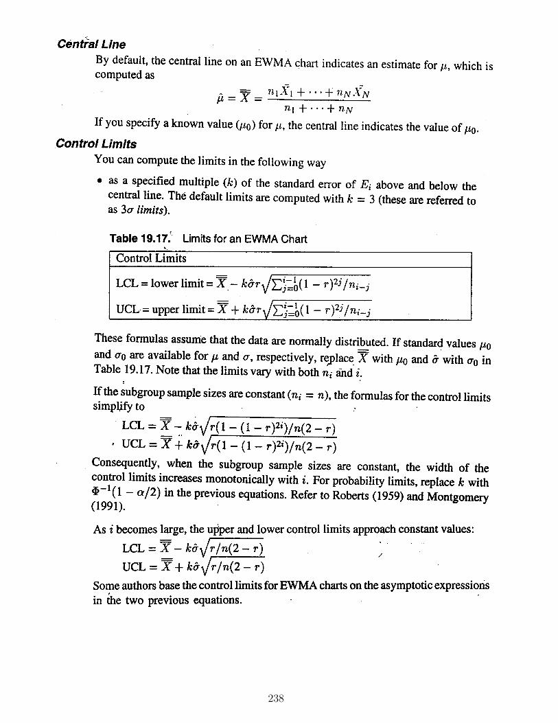
• When µ0 and σ2 are known, the EWMA chart is constructed by plotting zi versus the samplenumber i with control limits at:
UCL = µ0 + Lσ
√λ
2− λ(1− (1− λ)2i)
Centerline = µ0
LCL = µ0 − Lσ√
λ
2− λ(1− (1− λ)2i)
We will discuss the choice of L and λ later.
218

• Note thatλ
2− λ(1− (1− λ)2i
)−→ λ
2− λas i increases. Thus, after the EWMA chart has
been running for several samples, the control limits will approach the following steady-statevalues (called asymptotic control limits):
UCL = µ0 +
LCL = µ0 −
• It is recommended that exact control limits be used for small values of i because it will greatlyimprove the performance of the EWMA chart in detecting an off-target process very soon afterthe EWMA is started.
• SAS plots exact control limits by default. Plotting asymptotic control limits is an option.
• Example: Suppose λ = .25, L = 3, σ = 1, and µ0 = 0. Then, using the asymptotic variance,the control limits are
UCL = 0 + (3)(1)
√.25
1.75≈ LCL = 0− (3)(1)
√.25
1.75≈
The following table summarizes the EWMA calculation for 16 sample values (with comparisoncalculations for a tabular cusum with h = 5 and k = .5). Both the EWMA and the Cusumindicate an out-of-control signal on sample 16.
EWMA zi Tabular Cusumi xi λ = .25 with h = 5, k = .50 — z0 = 0 C+
i = 0 C−i = 0
1 1.0 .250 0.5 0.02 -0.5 .063 0.0 0.03 0.0 .047 0.0 0.04 -0.8 -.165 0.0 0.35 -0.8 -.324 0.0 0.66 -1.2 -.543 0.0 1.37 1.5 -.032 1.0 0.08 -0.6 -.174 0.0 0.19 1.0 .120 0.5 0.010 -0.9 -.135 0.0 0.411 1.2 .199 0.7 0.012 0.5 .274 0.7 0.013 2.6 .855 2.8 0.014 0.7 .817 3.0 0.015 1.1 .887 3.6 0.016 2.0 1.166 5.1 0.0
Sample EWMA calculations of zi = .25xi + .75zi−1
z1 = (.25)(1) + (.75)(0) = .25
z2 = (.25)(−.5) + (.75)(.25) = .0625 ≈ .063
z3 = (.25)(0) + (.75)(.0625) = .046875 ≈ .047
z4 = (.25)(−.8) + (.75)(.046875) = −.16484375 ≈ −.165
219

EWMA Chart Example
The MACONTROL Procedure
EWMA Chart Example
The MACONTROL Procedure
EWMA Chart Example
The MACONTROL Procedure
EWMA Parameters
Sigmas 3
Weight 0.25
Nominal Sample Size 1
Exponentially Weighted Moving Average Chart Summary for response
sample
SubgroupSample
SizeLower
Limit EWMASubgroup
MeanUpper
LimitLimit
Exceeded
1 1 -0.7500000 0.2500000 1.0000000 0.7500000
2 1 -0.9375000 0.0625000 -0.5000000 0.9375000
3 1 -1.0280490 0.0468750 0.0000000 1.0280490
4 1 -1.0756383 -0.1648438 -0.8000000 1.0756383
5 1 -1.1015041 -0.3236328 -0.8000000 1.1015041
6 1 -1.1157901 -0.5427246 -1.2000000 1.1157901
7 1 -1.1237462 -0.0320435 1.5000000 1.1237462
8 1 -1.1281968 -0.1740326 -0.6000000 1.1281968
9 1 -1.1306926 0.1194756 1.0000000 1.1306926
10 1 -1.1320941 -0.1353933 -0.9000000 1.1320941
11 1 -1.1328816 0.1984550 1.2000000 1.1328816
12 1 -1.1333244 0.2738412 0.5000000 1.1333244
13 1 -1.1335734 0.8553809 2.6000000 1.1335734
14 1 -1.1337134 0.8165357 0.7000000 1.1337134
15 1 -1.1337922 0.8874018 1.1000000 1.1337922
16 1 -1.1338365 1.1655513 2.0000000 1.1338365 Upper
220

EWMA Chart for Piston-Ring Diameterslambda weight=0.25 (mu, sigma known)
The MACONTROL Procedure
EWMA Chart for Piston-Ring Diameters with Resetslambda weight=0.25 (mu, sigma known)
The MACONTROL Procedure
221

EW
MA
Ch
art f
or P
isto
n-R
ing
Dia
met
ers
wit
h R
eset
sla
mbd
a w
eigh
t=0.
25 (
mu
, sig
ma
know
n)
Th
e M
AC
ON
TR
OL
Pro
cedu
re
EW
MA
Ch
art f
or P
isto
n-R
ing
Dia
met
ers
wit
h R
eset
sla
mbd
a w
eigh
t=0.
25 (
mu
, sig
ma
know
n)
Th
e M
AC
ON
TR
OL
Pro
cedu
re
EW
MA
Par
amet
ers
Sig
mas
3
Wei
ght
0.25
Nom
inal
Sam
ple
Siz
e5
Exp
onen
tial
ly W
eigh
ted
Mov
ing
Ave
rage
Ch
art
Su
mm
ary
for
dia
met
er
sam
ple
Su
bgr
oup
Sam
ple
Siz
eL
ower
Lim
itE
WM
AS
ub
grou
pM
ean
Up
per
Lim
itL
imit
Exc
eed
ed
1573.99832374.002550
74.01020074.001677
Upper
2573.99832374.000150
74.00060074.001677
3573.99790474.002113
74.00800074.002096
Upper
4573.99832374.000750
74.00300074.001677
5573.99790474.001413
74.00340074.002096
6573.99770173.999959
73.99560074.002299
7573.99759573.999970
74.00000074.002405
8573.99753773.999177
73.99680074.002463
9573.99750574.000433
74.00420074.002495
10573.99748773.999825
73.99800074.002513
11573.99747773.998418
73.99420074.002523
12573.99747273.999164
74.00140074.002528
13573.99746973.998973
73.99840074.002531
14573.99746773.996780
73.99020074.002533
Lower
15573.99832374.001500
74.00600074.001677
16573.99790474.000275
73.99660074.002096
17573.99770174.000406
74.00080074.002299
18573.99759574.002155
74.00740074.002405
19573.99753774.001166
73.99820074.002463
20573.99750574.003175
74.00920074.002495
Upper
21573.99832373.999950
73.99980074.001677
22573.99790474.000363
74.00160074.002096
23573.99770174.000872
74.00240074.002299
24573.99759574.001954
74.00520074.002405
25573.99753774.001015
73.99820074.002463
EW
MA
Ch
art f
or P
isto
n-R
ing
Dia
met
ers
lam
bda
wei
ght=
0.25
(m
u, s
igm
a kn
own
)
Th
e M
AC
ON
TR
OL
Pro
cedu
re
EW
MA
Ch
art f
or P
isto
n-R
ing
Dia
met
ers
lam
bda
wei
ght=
0.25
(m
u, s
igm
a kn
own
)
Th
e M
AC
ON
TR
OL
Pro
cedu
re
EW
MA
Par
amet
ers
Sig
mas
3
Wei
ght
0.25
Nom
inal
Sam
ple
Siz
e5
Exp
onen
tial
ly W
eigh
ted
Mov
ing
Ave
rage
Ch
art
Su
mm
ary
for
dia
met
er
sam
ple
Su
bgr
oup
Sam
ple
Siz
eL
ower
Lim
itE
WM
AS
ub
grou
pM
ean
Up
per
Lim
itL
imit
Exc
eed
ed
1573.99832374.002550
74.01020074.001677
Upper
2573.99790474.002063
74.00060074.002096
3573.99770174.003547
74.00800074.002299
Upper
4573.99759574.003410
74.00300074.002405
Upper
5573.99753774.003408
74.00340074.002463
Upper
6573.99750574.001456
73.99560074.002495
7573.99748774.001092
74.00000074.002513
8573.99747774.000019
73.99680074.002523
9573.99747274.001064
74.00420074.002528
10573.99746974.000298
73.99800074.002531
11573.99746773.998774
73.99420074.002533
12573.99746673.999430
74.00140074.002534
13573.99746573.999173
73.99840074.002535
14573.99746573.996929
73.99020074.002535
Lower
15573.99746573.999197
74.00600074.002535
16573.99746573.998548
73.99660074.002535
17573.99746573.999111
74.00080074.002535
18573.99746574.001183
74.00740074.002535
19573.99746574.000437
73.99820074.002535
20573.99746574.002628
74.00920074.002535
Upper
21573.99746574.001921
73.99980074.002535
22573.99746574.001841
74.00160074.002535
23573.99746574.001981
74.00240074.002535
24573.99746574.002785
74.00520074.002535
Upper
25573.99746574.001639
73.99820074.002535
222

DM ’LOG; CLEAR; OUT; CLEAR;’;ODS PRINTER PDF file=’C:\COURSES\ST528\ewma1.pdf’;* ODS LISTING;OPTIONS LS=76 PS=100 NONUMBER NODATE;
DATA piston;DO sample=1 TO 25;DO item=1 TO 5;
INPUT diameter @@;diameter = diameter + 70; OUTPUT;
END; END;LINES;4.030 4.002 4.019 3.992 4.008 3.995 3.992 4.001 4.011 4.004: : : : :
3.982 3.984 3.995 4.017 4.013;SYMBOL1 V=dot WIDTH=3 ;
PROC MACONTROL DATA=piston;EWMACHART diameter*sample=’1’ / WEIGHT = 0.25
mu0 = 74 sigma0=.005XSYMBOL = mu0 COUTHAXIS = 1 to 25TABLE TABLEOUTLIM; * MEANSYMBOL=plus;
LABEL diameter=’Diameter Ewma’sample = ’Piston Ring Sample’;
TITLE ’EWMA Chart for Piston-Ring Diameters’;TITLE2 ’lambda weight=0.25 (mu, sigma known)’;
PROC MACONTROL DATA=piston;EWMACHART diameter*sample=’1’ / WEIGHT = 0.25
mu0 = 74 sigma0=.005XSYMBOL = mu0 COUT RESETHAXIS = 1 to 25TABLE TABLEOUTLIM; * MEANSYMBOL=plus;
LABEL diameter=’Diameter Ewma’sample = ’Piston Ring Sample’;
TITLE ’EWMA Chart for Piston-Ring Diameters with Resets’;TITLE2 ’lambda weight=0.25 (mu, sigma known)’;RUN;
9.8 Estimating σ for a EWMA chart
• If unknown, the process standard deviation σ must be estimated from the data. In SAS, σ isestimated for the EWMA chart by a method similar to the MSSD used for cusum charts.
• Montgomery provides two alternative formulas for estimating σ:
1. If µ is specified, σ̂2 is the exponentially weighted mean square error (EWMS):
S2i =
– S2i is consistent (E(S2
i )→ σ2 as i→∞).
– S2i is approximately χ2 distributed with ν = (2− λ)/λ degrees of freedom.
– Thus, if σ0 is the in-control σ, we could plot√S2i versus the sample and set up
control limits for an exponentially weighted root mean square error control chart by:
UCL = σ0
√χ2ν,α/2
νand LCL = σ0
√χ2ν,1−α/2
ν
223

2. If µ is not specified, σ̂2 is the exponentially weighted moving variance (EWMV):
S2i =
• Because the points on the EWMA chart are weighted averages of the previous observations,successive EWMA points tend to be highly correlated with one another. As a result the out-of-control modified rules used with Shewhart charts cannot be applied to an EWMA chartbecause these rules apply to points that are statistically independent.
• From a SPC viewpoint, the EWMA is roughly equivalent to the cusum in its ability to monitora process and to detect assignable causes that result in a process shift. The EWMA, however,also provides a forecast of where the process mean will be at time or sample i+ 1. Thus, zi isa forecast of µ at time i+ 1.
• Thus, with an EWMA, we dynamically update our forecast as each new observation x arrives.
• The EWMA chart control limits can be used to determine when an adjustment in the processis necessary. We can determine how much to adjust the process at time i+ 1 by the differencezi − µ (the difference between our current estimate and the target value).
DM ’LOG; CLEAR; OUT; CLEAR;’;ODS PRINTER PDF file=’C:\COURSES\ST528\ewma2.pdf’;* ODS LISTING;OPTIONS LS=76 PS=100 NONUMBER NODATE;
DATA piston;DO sample=1 TO 25;DO item=1 TO 5;
INPUT diameter @@;diameter = diameter + 70; OUTPUT;
END; END;LINES;4.030 4.002 4.019 3.992 4.008 3.995 3.992 4.001 4.011 4.0043.988 4.024 4.021 4.005 4.002 4.002 3.996 3.993 4.015 4.0093.992 4.007 4.015 3.989 4.014 4.009 3.994 3.997 3.985 3.9933.995 4.006 3.994 4.000 4.005 3.985 4.003 3.993 4.015 3.9884.008 3.995 4.009 4.005 4.004 3.998 4.000 3.990 4.007 3.9953.994 3.998 3.994 3.995 3.990 4.004 4.000 4.007 4.000 3.9963.983 4.002 3.998 3.997 4.012 4.006 3.967 3.994 4.000 3.9844.012 4.014 3.998 3.999 4.007 4.000 3.984 4.005 3.998 3.9963.994 4.012 3.986 4.005 4.007 4.006 4.010 4.018 4.003 4.0003.984 4.002 4.003 4.005 3.997 4.000 4.010 4.013 4.020 4.0033.988 4.001 4.009 4.005 3.996 4.004 3.999 3.990 4.006 4.0094.010 3.989 3.990 4.009 4.014 4.015 4.008 3.993 4.000 4.0103.982 3.984 3.995 4.017 4.013;SYMBOL1 V=dot WIDTH=3 ;
PROC MACONTROL DATA=piston;EWMACHART diameter*sample=’1’ / WEIGHT = 0.25
mu0 = 74 RESETXSYMBOL = mu0 COUTHAXIS = 1 to 25 OUTLIMITS=limsetTABLE TABLEOUTLIM;
LABEL diameter=’Diameter Ewma’sample = ’Piston Ring Sample’;
TITLE ’EWMA Chart for Piston-Ring Diameters’;TITLE2 ’lambda weight=0.25 (sigma unknown)’;
PROC PRINT DATA = limset;RUN;
224

EWMA Chart for Piston-Ring Diameterslambda weight=0.25 (sigma unknown)
The MACONTROL Procedure
EWMA Chart for Piston-Ring Diameterslambda weight=0.25 (sigma unknown)
The MACONTROL Procedure
EWMA Parameters
Sigmas 3
Weight 0.25
Nominal Sample Size 5
Exponentially Weighted Moving Average Chart Summary for diameter
sample
SubgroupSample
SizeLower
Limit EWMASubgroup
MeanUpper
LimitLimit
Exceeded
1 5 73.996703 74.002550 74.010200 74.003297
2 5 73.995879 74.002063 74.000600 74.004121
3 5 73.995481 74.003547 74.008000 74.004519
4 5 73.995271 74.003410 74.003000 74.004729
5 5 73.995158 74.003408 74.003400 74.004842
6 5 73.995095 74.001456 73.995600 74.004905
7 5 73.995060 74.001092 74.000000 74.004940
8 5 73.995040 74.000019 73.996800 74.004960
9 5 73.995029 74.001064 74.004200 74.004971
10 5 73.995023 74.000298 73.998000 74.004977
11 5 73.995020 73.998774 73.994200 74.004980
12 5 73.995018 73.999430 74.001400 74.004982
13 5 73.995017 73.999173 73.998400 74.004983
14 5 73.995016 73.996929 73.990200 74.004984
15 5 73.995016 73.999197 74.006000 74.004984
16 5 73.995016 73.998548 73.996600 74.004984
17 5 73.995015 73.999111 74.000800 74.004985
18 5 73.995015 74.001183 74.007400 74.004985
19 5 73.995015 74.000437 73.998200 74.004985
20 5 73.995015 74.002628 74.009200 74.004985
21 5 73.995015 74.001921 73.999800 74.004985
22 5 73.995015 74.001841 74.001600 74.004985
23 5 73.995015 74.001981 74.002400 74.004985
24 5 73.995015 74.002785 74.005200 74.004985
25 5 73.995015 74.001639 73.998200 74.004985
225

EWMA Chart for Piston-Ring Diameterslambda weight=0.25 (sigma unknown)
The MACONTROL Procedure
EWMA Chart for Piston-Ring Diameterslambda weight=0.25 (sigma unknown)
EWMA Chart for Piston-Ring Diameterslambda weight=0.25 (sigma unknown)
Obs _VAR_ _SUBGRP_ _TYPE_ _LIMITN_ _ALPHA_ _SIGMAS_ _MEAN_ _STDDEV_ _WEIGHT_
1 diameter sample STDMU 5 .002699796 3 74 .009829977 0.25
226

***************************************************************************;*** In the manufacture of a metal clip, the gap between the ends of the ***;*** clip is a critical dimension. To monitor the process for change in ***;*** the average gap, subgroup samples of five clips are selected daily. ***;***************************************************************************;DM ’LOG; CLEAR; OUT; CLEAR;’;ODS LISTING;* ODS PRINTER PDF file=’C:\COURSES\ST528\ewma3.PDF’;OPTIONS NODATE NONUMBER LS=76 PS=54;
DATA clips1;INPUT day @@;DO i=1 TO 5;
INPUT gap @@ ; OUTPUT;END;
LINES;1 14.76 14.82 14.88 14.83 15.23 2 14.95 14.91 15.09 14.99 15.133 14.50 15.05 15.09 14.72 14.97 4 14.91 14.87 15.46 15.01 14.995 14.73 15.36 14.87 14.91 15.25 6 15.09 15.19 15.07 15.30 14.987 15.34 15.39 14.82 15.32 15.23 8 14.80 14.94 15.15 14.69 14.939 14.67 15.08 14.88 15.14 14.78 10 15.27 14.61 15.00 14.84 14.9411 15.34 14.84 15.32 14.81 15.17 12 14.84 15.00 15.13 14.68 14.9113 15.40 15.03 15.05 15.03 15.18 14 14.50 14.77 15.22 14.70 14.8015 14.81 15.01 14.65 15.13 15.12 16 14.82 15.01 14.82 14.83 15.0017 14.89 14.90 14.60 14.40 14.88 18 14.90 15.29 15.14 15.20 14.7019 14.77 14.60 14.45 14.78 14.91 20 14.80 14.58 14.69 15.02 14.8521 14.86 15.01 14.67 14.67 15.07 22 14.93 14.53 15.07 15.10 14.9823 15.27 14.90 15.12 15.10 14.80 24 15.02 15.21 14.93 15.11 15.2025 14.90 14.81 15.26 14.57 14.94 26 14.78 15.29 15.13 14.62 14.5427 14.78 15.15 14.61 14.92 15.07 28 14.92 15.31 14.82 14.74 15.2629 15.11 15.04 14.61 15.09 14.68 30 15.00 15.04 14.36 15.20 14.6531 14.99 14.76 15.18 15.04 14.82 32 14.90 14.78 15.19 15.06 15.0633 14.95 15.10 14.86 15.27 15.22 34 15.03 14.71 14.75 14.99 15.0235 15.38 14.94 14.68 14.77 14.83 36 14.95 15.43 14.87 14.90 15.3437 15.18 14.94 15.32 14.74 15.29 38 14.91 15.15 15.06 14.78 15.4239 15.34 15.34 15.41 15.36 14.96 40 15.12 14.75 15.05 14.70 14.74;SYMBOL1 V=dot WIDTH=3;
PROC MACONTROL DATA=clips1 ;EWMACHART gap*day=’1’ / WEIGHT = 0.3 COUT
TABLE TABLEID TABLEOUTLIMXSUMBOL = mu0;
LABEL gap = ’Gap in Clip’day = ’Day’;
TITLE ’EWMA Chart -- weight=0.3 (mu, sigma unknown)’;RUN;
PROC MACONTROL DATA=clips1 ;EWMACHART gap*day=’1’ / WEIGHT = 0.5 COUT
TABLE TABLEID TABLEOUTLIMXSUMBOL = mu0;
LABEL gap = ’Gap in Clip’day = ’Day’;
TITLE ’EWMA Chart -- weight=0.5 (mu, sigma unknown)’;RUN;
227

EWMA Chart -- weight=0.3 (mu, sigma unknown)
The MACONTROL Procedure
EWMA Chart -- weight=0.5 (mu, sigma unknown)
The MACONTROL Procedure
228

EWMA Chart -- weight=0.3 (mu, sigma unknown)
The MACONTROL Procedure
EWMA Parameters
Sigmas 3Weight 0.3Nominal Sample Size 5
Exponentially Weighted Moving Average Chart Summary for gap
SubgroupSample Lower Subgroup Upper Limit
day Size Limit EWMA Mean Limit Exceeded
1 5 14.875545 14.946980 14.904000 15.0552552 5 14.855718 14.967086 15.014000 15.0750823 5 14.847211 14.936760 14.866000 15.0835894 5 14.843258 14.970132 15.048000 15.0875425 5 14.841368 14.986292 15.024000 15.0894326 5 14.840452 15.028205 15.126000 15.0903487 5 14.840005 15.085743 15.220000 15.0907958 5 14.839787 15.030620 14.902000 15.0910139 5 14.839680 14.994434 14.910000 15.091120
10 5 14.839628 14.975704 14.932000 15.09117211 5 14.839602 15.011793 15.096000 15.09119812 5 14.839590 14.981855 14.912000 15.09121013 5 14.839584 15.028698 15.138000 15.09121614 5 14.839581 14.959489 14.798000 15.09121915 5 14.839579 14.954842 14.944000 15.09122116 5 14.839578 14.937190 14.896000 15.09122217 5 14.839578 14.876233 14.734000 15.09122218 5 14.839578 14.927163 15.046000 15.09122219 5 14.839578 14.859614 14.702000 15.09122220 5 14.839578 14.838130 14.788000 15.091222 Lower21 5 14.839578 14.843491 14.856000 15.09122222 5 14.839578 14.867044 14.922000 15.09122223 5 14.839578 14.918331 15.038000 15.09122224 5 14.839578 14.971031 15.094000 15.09122225 5 14.839578 14.948522 14.896000 15.09122226 5 14.839578 14.925565 14.872000 15.09122227 5 14.839578 14.919696 14.906000 15.09122228 5 14.839578 14.946787 15.010000 15.09122229 5 14.839578 14.934551 14.906000 15.09122230 5 14.839578 14.909186 14.850000 15.09122231 5 14.839578 14.923830 14.958000 15.09122232 5 14.839578 14.946081 14.998000 15.09122233 5 14.839578 14.986257 15.080000 15.09122234 5 14.839578 14.960380 14.900000 15.09122235 5 14.839578 14.948266 14.920000 15.09122236 5 14.839578 14.993186 15.098000 15.09122237 5 14.839578 15.023430 15.094000 15.09122238 5 14.839578 15.035601 15.064000 15.09122239 5 14.839578 15.109521 15.282000 15.091222 Upper40 5 14.839578 15.038265 14.872000 15.091222
229

EWMA Chart -- weight=0.5 (mu, sigma unknown)
The MACONTROL Procedure
EWMA Parameters
Sigmas 3Weight 0.5Nominal Sample Size 5
Exponentially Weighted Moving Average Chart Summary for gap
SubgroupSample Lower Subgroup Upper Limit
day Size Limit EWMA Mean Limit Exceeded
1 5 14.815642 14.934700 14.904000 15.1151582 5 14.797965 14.974350 15.014000 15.1328353 5 14.793830 14.920175 14.866000 15.1369704 5 14.792812 14.984088 15.048000 15.1379885 5 14.792558 15.004044 15.024000 15.1382426 5 14.792495 15.065022 15.126000 15.1383057 5 14.792479 15.142511 15.220000 15.138321 Upper8 5 14.792475 15.022255 14.902000 15.1383259 5 14.792474 14.966128 14.910000 15.138326
10 5 14.792474 14.949064 14.932000 15.13832611 5 14.792474 15.022532 15.096000 15.13832612 5 14.792474 14.967266 14.912000 15.13832613 5 14.792474 15.052633 15.138000 15.13832614 5 14.792474 14.925316 14.798000 15.13832615 5 14.792474 14.934658 14.944000 15.13832616 5 14.792474 14.915329 14.896000 15.13832617 5 14.792474 14.824665 14.734000 15.13832618 5 14.792474 14.935332 15.046000 15.13832619 5 14.792474 14.818666 14.702000 15.13832620 5 14.792474 14.803333 14.788000 15.13832621 5 14.792474 14.829667 14.856000 15.13832622 5 14.792474 14.875833 14.922000 15.13832623 5 14.792474 14.956917 15.038000 15.13832624 5 14.792474 15.025458 15.094000 15.13832625 5 14.792474 14.960729 14.896000 15.13832626 5 14.792474 14.916365 14.872000 15.13832627 5 14.792474 14.911182 14.906000 15.13832628 5 14.792474 14.960591 15.010000 15.13832629 5 14.792474 14.933296 14.906000 15.13832630 5 14.792474 14.891648 14.850000 15.13832631 5 14.792474 14.924824 14.958000 15.13832632 5 14.792474 14.961412 14.998000 15.13832633 5 14.792474 15.020706 15.080000 15.13832634 5 14.792474 14.960353 14.900000 15.13832635 5 14.792474 14.940176 14.920000 15.13832636 5 14.792474 15.019088 15.098000 15.13832637 5 14.792474 15.056544 15.094000 15.13832638 5 14.792474 15.060272 15.064000 15.13832639 5 14.792474 15.171136 15.282000 15.138326 Upper40 5 14.792474 15.021568 14.872000 15.138326
230

EWMA Example with Unequal Sample Sizes
DM ’LOG; CLEAR; OUT; CLEAR;’;
* ODS PRINTER PDF file=’C:\COURSES\ST528\EWMA4.PDF’;
OPTIONS NODATE NONUMBER;
************************************;
*** UNEQUAL SAMPLE SIZE EXAMPLE ***;
************************************;
DATA clips4;
INPUT day @@;
DO i=1 TO 5;
INPUT gap @@; OUTPUT;
END;
LINES;
1 14.93 14.65 14.87 15.11 15.18
2 15.06 14.95 14.91 15.14 15.41
3 14.90 14.90 14.96 15.26 15.18
4 15.25 14.57 15.33 15.38 14.89
7 14.68 14.63 14.72 15.32 14.86
8 14.48 14.88 14.98 14.74 15.48
9 14.99 15.16 15.02 15.53 14.66
10 14.88 15.44 15.04 15.10 14.89
11 15.14 15.33 14.75 15.23 14.64
14 15.46 15.30 14.92 14.58 14.68
15 15.23 14.63 . . .
16 15.13 15.25 . . .
17 15.06 15.25 15.28 15.30 15.34
18 15.22 14.77 15.12 14.82 15.29
21 14.95 14.96 14.65 14.87 14.77
22 15.01 15.11 15.11 14.79 14.88
23 14.97 15.50 14.93 15.13 15.25
24 15.23 15.21 15.31 15.07 14.97
25 15.08 14.75 14.93 15.34 14.98
28 15.07 14.86 15.42 15.47 15.24
29 15.27 15.20 14.85 15.62 14.67
30 14.97 14.73 15.09 14.98 14.46
;
SYMBOL1 V=dot WIDTH=3;
PROC MACONTROL DATA=clips4;
EWMACHART gap*day=’1’ / WEIGHT = 0.3 COUT
TABLE TABLEID TABLEOUTLIM;
LABEL gap = ’Gap in Clip’
day = ’April’;
TITLE ’EWMA Chart -- weight=0.3 (unequal sample sizes)’;
RUN;
231

EWMA Chart -- weight=0.3 (unequal sample sizes)
The MACONTROL Procedure
EW
MA
Ch
art -
- w
eigh
t=0.
3 (u
neq
ual
sam
ple
size
s)
Th
e M
AC
ON
TR
OL
Pro
cedu
re
EW
MA
Ch
art -
- w
eigh
t=0.
3 (u
neq
ual
sam
ple
size
s)
Th
e M
AC
ON
TR
OL
Pro
cedu
re
EW
MA
Par
amet
ers
Sig
mas
3
Wei
ght
0.3
Nom
inal
Sam
ple
Siz
eVarying
Exp
onen
tial
ly W
eigh
ted
Mov
ing
Ave
rage
Ch
art
Su
mm
ary
for
gap
day
Su
bgr
oup
Sam
ple
Siz
eL
ower
Lim
itE
WM
AS
ub
grou
pM
ean
Up
per
Lim
itL
imit
Exc
eed
ed
1514.92871415.009169
14.94800015.142055
2514.90517715.034618
15.09400015.165593
3514.89507715.036233
15.04000015.175692
4514.89038515.050563
15.08400015.180384
7514.88814114.987994
14.84200015.182629
8514.88705314.965196
14.91200015.183716
9514.88652314.997237
15.07200015.184246
10514.88626415.019066
15.07000015.184505
11514.88613815.018746
15.01800015.184632
14514.88607515.009522
14.98800015.184694
15214.83696514.985666
14.93000015.233804
16214.81689415.046966
15.19000015.253875
17514.84891715.106676
15.24600015.221852
18514.86681415.087873
15.04400015.203955
21514.87631715.013511
14.84000015.194452
22514.88118715.003458
14.98000015.189582
23514.88363115.049221
15.15600015.187139
24514.88484215.081854
15.15800015.185927
25514.88544015.062098
15.01600015.185330
28514.88573315.107069
15.21200015.185036
29514.88587715.111548
15.12200015.184892
30514.88594815.031884
14.84600015.184821
232

9.9 Design of the EWMA Control Chart
• The design parameters of the EWMA chart are L (the multiple of σzi used in the controllimits) and λ (the weighting constant).
• It is possible to choose L and λ so that the ARL performance of the EWMA chart closelyapproximates the performance of a cusum ARL for detecting small shifts.
• The optimal EWMA design procedure would be to specify a desired in-control ARL, themagnitude of the shift to be detected quickly, and an out-of-control ARL corresponding tothis shift. Then, determine if there exist L and λ values satisfying these conditions.
• Typically, we take the same approach taken with determining cusum parameters h and k.That is, we use EWMA ARL tables to find reasonable L and λ parameter values that bestmeet our desired ARL conditions. You have been supplied with tables of ARLs taken fromthe SAS QC manual (r = λ, k = L).
• Montgomery recommends the following:
1. Use smaller values of λ to detect smaller shifts.
2. Values of λ in the interval 0.05 ≤ λ ≤ 0.25 work well in practice (with λ = 0.05, 0.10, 0.20being commonly used values).
3. Using L = 3 works reasonably well with larger values of λ.
4. Using 2.6 ≤ L ≤ 2.8 works reasonably well with smaller values of λ (λ ≤ 0.10).
5. λ = .10 and L = 2.7 produces a EWMA chart approximately equivalent to a cusumchart with h = 5 and k = .5.
6. If λ > 0.10, the EWMA is often superior to a cusum for large shifts.
7. To improve the sensitivity of the EWMA chart (or cusum chart) to detect large shiftswithout sacrificing the ability to detect small shifts quickly, combine a Shewhart chartwith the EWMA (or cusum). The combined Shewhart-EWMA (or combined Shewhart-Cusum) procedures are effective against both large and small shifts.
• There is also the EWMAARL function in SAS that will generate ARLs for a given shift δσ,L, and λ values.
OPTIONS LS=72 PS=54 NODATE NONUMBER;
*** Designing an EWMA Chart;
DATA ewmaarl;
DO L = 3 TO 3.1 BY .1;
DO lambda = .05 to 1 BY .05;
arl0 = EWMAARL(0,lambda,L);
arl1 = EWMAARL(1,lambda,L);
arl2 = EWMAARL(2,lambda,L); *** 2 sigma shift for comparison;
* IF (148 le arl0 le 152) and (8.5 le arl1 le 9.5) THEN OUTPUT;
OUTPUT;
END; END;
PROC PRINT DATA=ewmaarl;
RUN;
233

The SAS System
Obs L lambda arl0 arl1 arl2
1 3.0 0.05 1383.62 13.5161 6.004672 3.0 0.10 842.15 11.3840 4.669503 3.0 0.15 655.01 10.8303 4.108964 3.0 0.20 559.87 10.8359 3.800855 3.0 0.25 502.90 11.1543 3.616776 3.0 0.30 465.55 11.6986 3.506357 3.0 0.35 439.70 12.4349 3.445538 3.0 0.40 421.16 13.3518 3.422269 3.0 0.45 407.57 14.4500 3.43069
10 3.0 0.50 397.46 15.7378 3.4685011 3.0 0.55 389.89 17.2287 3.5356412 3.0 0.60 384.21 18.9408 3.6337613 3.0 0.65 379.96 20.8959 3.7660314 3.0 0.70 376.81 23.1192 3.9371415 3.0 0.75 374.50 25.6391 4.1534616 3.0 0.80 372.85 28.4873 4.4233617 3.0 0.85 371.70 31.6983 4.7576218 3.0 0.90 370.95 35.3093 5.1699819 3.0 0.95 370.53 39.3605 5.6778020 3.0 1.00 . . .
21 3.1 0.05 1856.77 14.1078 6.2124022 3.1 0.10 1131.69 11.9924 4.8388223 3.1 0.15 885.42 11.5272 4.2664424 3.1 0.20 760.52 11.6638 3.9553925 3.1 0.25 685.96 12.1514 3.7732326 3.1 0.30 637.32 12.9044 3.6689227 3.1 0.35 603.82 13.8922 3.6182228 3.1 0.40 579.96 15.1086 3.6090029 3.1 0.45 562.60 16.5599 3.6355830 3.1 0.50 549.80 18.2612 3.6961031 3.1 0.55 540.31 20.2336 3.7912632 3.1 0.60 533.26 22.5033 3.9237433 3.1 0.65 528.06 25.1014 4.0980934 3.1 0.70 524.25 28.0630 4.3207835 3.1 0.75 521.49 31.4272 4.6004536 3.1 0.80 519.55 35.2369 4.9483037 3.1 0.85 518.22 39.5387 5.3786638 3.1 0.90 517.37 44.3824 5.9096939 3.1 0.95 516.89 49.8214 6.5642640 3.1 1.00 . . .
234

251
235

247
236

248
237
249
238

Choosing the Value of the Weight Parameter
250
239
Related Documents