Dartmouth College Dartmouth College Dartmouth Digital Commons Dartmouth Digital Commons Dartmouth College Undergraduate Theses Theses, Dissertations, and Graduate Essays Spring 6-1-2021 Exploring the Long Tail Exploring the Long Tail Joseph H. Hajjar Dartmouth College, [email protected] Follow this and additional works at: https://digitalcommons.dartmouth.edu/senior_theses Part of the Artificial Intelligence and Robotics Commons, and the Data Science Commons Recommended Citation Recommended Citation Hajjar, Joseph H., "Exploring the Long Tail" (2021). Dartmouth College Undergraduate Theses. 227. https://digitalcommons.dartmouth.edu/senior_theses/227 This Thesis (Undergraduate) is brought to you for free and open access by the Theses, Dissertations, and Graduate Essays at Dartmouth Digital Commons. It has been accepted for inclusion in Dartmouth College Undergraduate Theses by an authorized administrator of Dartmouth Digital Commons. For more information, please contact [email protected].

Welcome message from author
This document is posted to help you gain knowledge. Please leave a comment to let me know what you think about it! Share it to your friends and learn new things together.
Transcript

Dartmouth College Dartmouth College
Dartmouth Digital Commons Dartmouth Digital Commons
Dartmouth College Undergraduate Theses Theses, Dissertations, and Graduate Essays
Spring 6-1-2021
Exploring the Long Tail Exploring the Long Tail
Joseph H. Hajjar Dartmouth College, [email protected]
Follow this and additional works at: https://digitalcommons.dartmouth.edu/senior_theses
Part of the Artificial Intelligence and Robotics Commons, and the Data Science Commons
Recommended Citation Recommended Citation Hajjar, Joseph H., "Exploring the Long Tail" (2021). Dartmouth College Undergraduate Theses. 227. https://digitalcommons.dartmouth.edu/senior_theses/227
This Thesis (Undergraduate) is brought to you for free and open access by the Theses, Dissertations, and Graduate Essays at Dartmouth Digital Commons. It has been accepted for inclusion in Dartmouth College Undergraduate Theses by an authorized administrator of Dartmouth Digital Commons. For more information, please contact [email protected].

Exploring the Long Tail:
A Survey of Movie Embeddings
Joseph H. Hajjar
Advisor: Daniel Rockmore
June 1, 2021
Undergraduate Honors Thesis in Computer Science
Dartmouth College
Abstract
The migration of datasets online has created a near-infinite inventory for big name
retailers such as Amazon and Netflix, giving rise to recommendation systems to assist
users in navigating the massive catalog. This has also allowed for the possibility of
retailers storing much less popular, uncommon items which would not appear in a
more traditional brick-and-mortar setting due to the cost of storage. Nevertheless,
previous work has highlighted the profit potential which lies in the so-called “long
tail” of niche, unpopular items. Unfortunately, due to the limited amount of data in
this subset of the inventory, recommendation systems often struggle to make useful
suggestions within the long tail, lending them prone to a popularity bias.
Our work explores different approaches which recommendation systems typically
employ and evaluate the performance of each approach on various subsets of the Net-
flix Prize data to the end of determining where each approach performs best. We
survey collaborative filtering approaches, content-based filtering approaches, and hy-
brid mechanisms utilizing both of the previous methods. We analyze their behavior on
the most popular items, the least popular items, and a composite of the two subsets,
and we judge their performance based on the quality of the clusters they produce.
KEY WORDS: collaborative filtering, content based filtering, recommendation sys-
tems, clustering, machine learning
1

Contents
1 Introduction 4
2 Objective 4
3 Background 5
3.1 Content-Based Filtering . . . . . . . . . . . . . . . . . . . . . . . . . . . . . 5
3.2 Collaborative Filtering . . . . . . . . . . . . . . . . . . . . . . . . . . . . . . 6
4 Motivation and Related Work 6
5 Dataset 8
5.1 Enriching the Dataset . . . . . . . . . . . . . . . . . . . . . . . . . . . . . . 8
6 Methodology 9
6.1 Similarity and Dissimilarity . . . . . . . . . . . . . . . . . . . . . . . . . . . 11
6.2 Spectral Clustering . . . . . . . . . . . . . . . . . . . . . . . . . . . . . . . . 12
6.3 Ratings-Based Approaches . . . . . . . . . . . . . . . . . . . . . . . . . . . . 13
6.3.1 Cosine Similarity . . . . . . . . . . . . . . . . . . . . . . . . . . . . . 13
6.3.2 Altitude similarity . . . . . . . . . . . . . . . . . . . . . . . . . . . . 13
6.4 Content-Based Approaches . . . . . . . . . . . . . . . . . . . . . . . . . . . . 14
6.4.1 Topic Modeling . . . . . . . . . . . . . . . . . . . . . . . . . . . . . . 15
6.4.2 Kullback–Leibler Divergence . . . . . . . . . . . . . . . . . . . . . . . 16
6.5 Hybrid Approaches . . . . . . . . . . . . . . . . . . . . . . . . . . . . . . . . 17
6.5.1 Chordal Distance . . . . . . . . . . . . . . . . . . . . . . . . . . . . . 18
6.6 Graph Sparsification . . . . . . . . . . . . . . . . . . . . . . . . . . . . . . . 19
7 Evaluation 20
7.1 Customized Homogeneity Metric . . . . . . . . . . . . . . . . . . . . . . . . 21
2

8 Results 21
8.1 Ratings-Based Results . . . . . . . . . . . . . . . . . . . . . . . . . . . . . . 22
8.2 Comparing Ratings-Based and Content-Based Results . . . . . . . . . . . . . 23
8.3 Hybrid Results . . . . . . . . . . . . . . . . . . . . . . . . . . . . . . . . . . 25
9 Conclusion 26
10 Future Work 27
A Graph Visualizations 35
3
1 Introduction
Recommendation systems are born out of a need for assistance in navigating massive datasets.
In this new age of information, there are two primary ways in which these interactions occur.
One way is through a query, user-driven, while the other is through an algorithm, driven
instead by the system. Because of the size of these datasets, it’s difficult for the user to know
where to begin their search. The user may have an idea of a general location where they
want their search to take them, but given the often overwhelming amount of destinations
available, the task can feel overwhelming.
To ease this process, recommendation systems have the power to suggest user-specific
content which may bring to light items for which a user may not have considered to search
specifically. This is particularly useful since retailers are now able to store less popular,
more obscure items which reside in the so-called “long tail” of popularity. This means that
through the use of recommendation systems, retailers are able to cater to larger audiences,
both on the customer side and the supply side.
As a result, recommendation systems can be portrayed as a promising business oppor-
tunity due to their ability to produce user-specific suggestions, targeting end users precisely
while eliminating the likelihood of advertising to which a user would respond poorly [1, 2].
Indeed, Netflix was so keen to improve the quality of its engine that it famously held a com-
petition (The Netflix Prize) awarding one million dollars to the research group which could
come up with the greatest reduction in root mean squared error (RMSE) to its contemporary
algorithm Cinematch [3].
2 Objective
In this paper, we take a look at two common ways which recommendation systems make their
suggestions, content-based filtering and ratings-based filtering (explained in Sections 3.1 and
4

3.2, respectively), and evaluate the quality of the approaches on three different subsets of
the dataset: the most popular items, the least popular items, and a composite of the most
popular items and the least popular items (more on the dataset in Section 5). Following this
survey, we take a look at different hybrid systems which take into account both the ratings
and content based metrics. We compare the performance of each approach and metric by
the quality of the clusters that Algorithm 1 produces. The goal of the paper is to determine
on which subsets of the data different approaches perform best - paying close attention to
which approaches do the best within the least popular items and which approaches connect
the most and least popular items most effectively.
3 Background
In the following sections, we introduce terminology relevant to the analysis, and describe
two of the most popular methods which recommendation systems employ.
3.1 Content-Based Filtering
Content-based filtering (CB) makes recommendations based on a user profile, indicating a
user’s preference for certain features, and the amount to which these features are present
in the items [4, 5]. The user profile can be built through a questionnaire when the user
creates their account, or it can be learned through user’s actions [6]. In this context, items
are embedded based on some notion of their content, users represented by their user profile,
and the similarity between these two is leveraged by recommendation engines to produce
suggestions [4, 7].
CB performs well where items can be described by a set of features, but is not applicable
to all itemsets. CB also benefits from being able to make recommendations about new items
(the “item cold-start problem”). However, it can lead to overspecialization as only items
with certain features will be recommended, which can box users into a corner [7].
5
3.2 Collaborative Filtering
Alternatively, to produce recommendations with collaborative filtering (CF), the system
leverages information from other users to find those which have the most consistent rating
pattern to the active user through some correlation measure (such as k-Nearest Neighbors
or Pearson Correlation) [6, 8]. Then, items which similar users rate positively will be rec-
ommended to the active user. Once again, the notion of similarity is up to the system to
decide.
A common approach used to this end, popularized during the Netflix Prize competition,
is matrix factorization [9]. To understand this approach, we can create the n × m ratings
matrix R. Each entry R(i, j) represents user i’s rating of item j. This matrix is factored
to produce a n × d matrix U and a d ×m matrix V . Each column in the matrix V can be
thought of as representing item j in some d-dimensional space, and each row in matrix U can
be thought of as representing user i in the same d-dimensional space. These representations
can be used to find similar users to the active user and similar items to the active user’s
highly rated items [10].
In this context, items are embedded based on their ratings, completely independent of
what the item actually is. Therefore, CF is advantageous in that it can be applied to any
itemset - the algorithm does not rely on the content of the items, only their ratings. It has
been empirically shown to produce high quality recommendations and generally outperforms
content-based filtering [11, 12, 13]. However, since it is reliant on rating information, CF
struggles with the “cold-start problem” for both items and users.
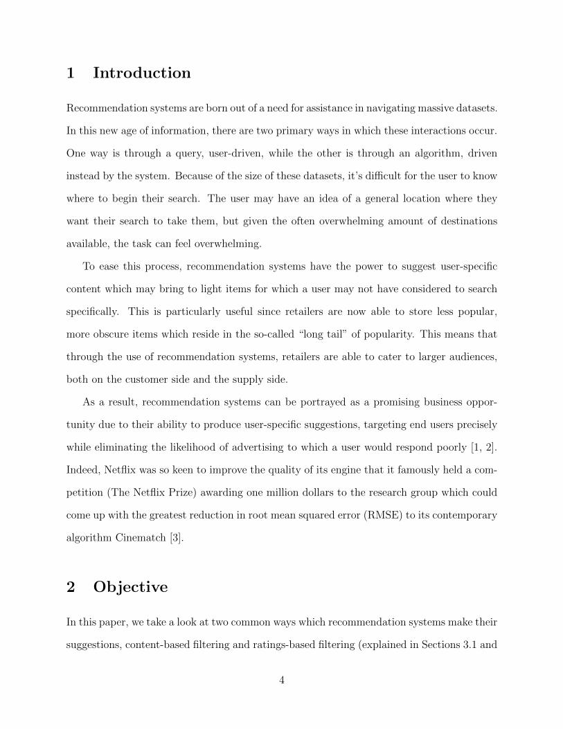
4 Motivation and Related Work
Many recommendation systems struggle to deal with items which are lightly reviewed. An-
derson coined the term “long tail” in [1] to refer to the items in a retailer’s inventory which
6
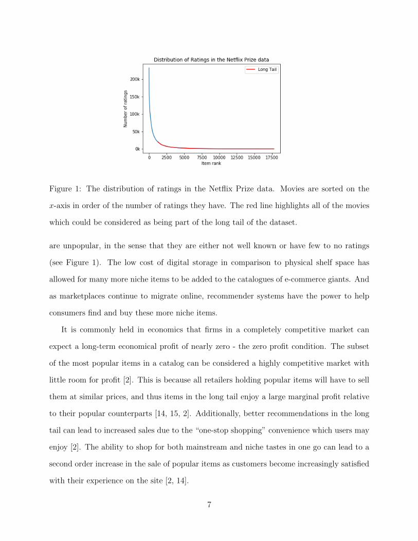
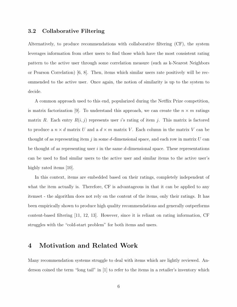
Figure 1: The distribution of ratings in the Netflix Prize data. Movies are sorted on the
x-axis in order of the number of ratings they have. The red line highlights all of the movies
which could be considered as being part of the long tail of the dataset.
are unpopular, in the sense that they are either not well known or have few to no ratings
(see Figure 1). The low cost of digital storage in comparison to physical shelf space has
allowed for many more niche items to be added to the catalogues of e-commerce giants. And
as marketplaces continue to migrate online, recommender systems have the power to help
consumers find and buy these more niche items.
It is commonly held in economics that firms in a completely competitive market can
expect a long-term economical profit of nearly zero - the zero profit condition. The subset
of the most popular items in a catalog can be considered a highly competitive market with
little room for profit [2]. This is because all retailers holding popular items will have to sell
them at similar prices, and thus items in the long tail enjoy a large marginal profit relative
to their popular counterparts [14, 15, 2]. Additionally, better recommendations in the long
tail can lead to increased sales due to the “one-stop shopping” convenience which users may
enjoy [2]. The ability to shop for both mainstream and niche tastes in one go can lead to a
second order increase in the sale of popular items as customers become increasingly satisfied
with their experience on the site [2, 14].
7

Thus, the question of how to bridge the gap between the head and the tail of the dataset
is one relevant for all parties involved: retailers benefit from a more robust bridge as large
share of their profits come from sales in the long tail, creators benefit from being able to find
people who enjoy their content, and users are able to have their unique, uncommon tastes
met [1, 16].
5 Dataset
Our analysis is carried out on the famous Netflix Prize dataset1. This dataset consists of
around 100 million ratings from more than 480 thousand distinct Netflix users on almost 18
thousand different movies, collected between October 1998 and December 2005. The ratings
are integral from 1 to 5 where 1 indicates a negative rating and 5 indicates a positive rating.
The dataset was formed by randomly sampling a subset of all users who had rated at least 20
movies in the time period where ratings were collected. The data was collected in a manner
so as to accurately reflect the distribution of Netflix ratings over that same period of time
[17].
5.1 Enriching the Dataset
With regards to movie metadata, the Netflix Prize dataset leaves a lot to be desired - only
the movie titles and their years of release were given along with the ratings information.
We augmented the data by pulling genres and plot summaries from in full Internet Movie
Database (IMDb)2. Genre information is submitted by users before being approved by indus-
try professionals on IMDb, meanwhile plot summaries can be submitted by any individual3.
Preliminary efforts to merge the datasets (matching on title and year) yielded disappointing,
1https://www.kaggle.com/netflix-inc/netflix-prize-data2https://www.imdb.com/interfaces/3https://help.imdb.com/article/contribution/titles/genres/GZDRMS6R742JRGAG
8

underwhelming intersections.
To investigate further, we took a random sample of 100 Netflix movies and manually
queried the IMDb database to discover that, within our random sample, 46 percent of the
Netflix titles were perfect matches (same title and year), 10 percent of the Netflix movies had
slightly different titles in the IMDb dataset (e. g. Fidel Castro vs Fidel Castro: American
Experience), and 8 percent of the Netflix movies had release years which were off by 1 or 2
years in the IMDb dataset.
Using the IMDbPy Python package, we were able to find the largest intersection between
these two datasets. The package mimicks a search on IMDb’s website, which was useful given
that many of the titles in the IMDb database differed only slightly from those in the Netflix
data. For each movie, out of the first 100 results of the IMDb query, we first looked for
movies which matched exactly on the Netflix year y. If no movies matched, then we looked
for movies which matched on y + 1, and again if no movies matched, we looked for movies
which matched on y − 1. While we had found that some titles were off by 2 years between
the datasets, we restricted our search to titles off by 1 year so as to limit false positive finds
in the IMDb dataset. For movies which had more than 1 plot summary submitted, we chose
to scrape the longest one. We were able to find genre information for 14262 of the 17770
movies and plot summaries for 13350 of the 17770 movies. Previous attempts4 to combine
the two datasets (Netflix Prize and IMDb) yielded much smaller intersections, but those had
worked on more exact title matching [18].
6 Methodology
We evaluated three different ways of moving through the movie space. The first was using
exclusively the user ratings, the second was using the content of the movie plot summaries,
and the last was a hybrid of the first two methods exploring different weights for the content
4https://github.com/bmxitalia/netflix-prize-with-genres
9
Figure 2: Visual representation of the exploration of the dataset.
and the ratings.
For each of the mentioned methods we explored their performance on three different
subsets of the movies. The first was the most popular 2,000 movies, the second was the
least popular 2,000 movies, and the final subset was a combination of the most popular
1,000 movies and the least popular 1,000 movies where popularity was measured in the
number of ratings a movie had independent of the ratings’ values5. This would give us a
good sense of where in the dataset each method was most likely to yield the best results.
In particular, it would give us a sense of which metrics could help bridge the gap in the
quality of recommendations between the most popular items and the least popular ones,
which metrics could most effectively bring lightly reviewed items to the surface.
To quantitatively evaluate the performance of each method, we applied spectral clus-
tering to the data, which would produce labels for movies which showed the most affinity
to each other, and compared these labels to the genre labels we pulled from IMDb. The
spectral clustering algorithm along with the metrics we used to evaluate their performance
are described in Section 6.2.
5It is worthwhile to note that since not all movies had information from IMDb with which to verify our
results, we took the subset of the listed sets which had data from IMDb. This shrank the size of each
subset to 1608 for the most popular movies, 1131 for the least popular movies, and 1368 for the top/bottom
composite.
10

Lastly, for a more visual, qualitative assessment of the metrics, we visualized the data as
a graph to find where the movies fit in the space. Given the overwhelming number of edges,
in a fully-connected graph with 2,000 nodes, we applied a various sparsification techniques
to find a backbone to the network. The first was a naive global threshold while the second
was a more intricate way of retaining only locally significant edges described in Section 6.6.
Aside from Section 6.6, visualizations will not be discussed for the rest of the paper, however
screenshots of the graphs produced can be found in Appendix A.
6.1 Similarity and Dissimilarity
A useful question to consider when performing data analysis is: when are two things similar
or dissimilar? The ability to answer this question greatly reduces the complexity of a dataset
[19].
Let xi and xj be two n-dimensional vectors where n is the number of features. These
vectors can be considered to be n-dimensional embeddings of movies i and j. A similarity
measure is a function which returns high values for two vectors xi and xj if xi and xj are
similar and low values if they are not. Likewise, a dissimilarity measure is a function which
returns high values if xi and xj are dissimilar and low values if they are similar. More
precisely, similarity measures will generally adhere to the following properties:
1. Every vector xi is maximally similar to itself.
2. If xi is similar to xj, then xj is equally similar to xj.
3. If xi is similar to xj and xj is similar to xk, then xi should be similar to xk.
The analogous properties are followed by dissimilarity measures. Our work explores different
similarity and dissimilarity metrics.
11

Algorithm 1 Normalized Spectral Clustering (S, k)
1: Construct the fully connected similarity graph G(V,E) where each edge eij = S(i, j).2: Let W be the weighted adjacency matrix of graph G.
3: Let D be the diagonal degree matrix
(d1
...dn
)where each di represents the degree of
node i.4: Compute the unnormalized Laplacian matrix L = D −W .5: Compute the first k generalized eigenvectors u1, . . . , uk of the generalized eigenproblemLu = λDu.
6: Define U ∈ Rn×k as the matrix with eigenvectors u1, . . . , uk as columns.7: Let yi be the i−th row of the matrix U for i = 1, . . . , n.8: Cluster the points k-dimensional points y1, . . . , yk with k-means to form clustersC1, . . . , Ck
9: return a partition of the data A1, . . . , Ak where Ai = {j | yj ∈ Ci}
6.2 Spectral Clustering
Spectral clustering refers to a family of clustering algorithms which leverage the eigenvalues
of the similarity matrix to form clusters in a graph. A similarity matrix S is a matrix
in Rn×n where n is the number of samples being compared, and each entry S(i, j) stores a
value representing the similarity between samples i and j. Due to the symmetry of similarity
measures, the matrix S is symmetric.
The clustering applied to the dataset was the normalized spectral clustering algorithm
popularized by Shi and Malik [20]. The algorithm takes as input the similarity matrix
S ∈ Rn×n and an integer k where n is the number of samples to cluster and k is the number
of clusters to produce. The procedure is described in Algorithm 1. Although the algorithm
described uses the unnormalized Laplacian matrix, it uses the generalized eigenvalues of the
unnormalized Laplacian, which correspond to the eigenvectors of the normalized Laplacian
matrix L = I − D−1W [21]. Thus, it is referred to as a normalized spectral clustering
algorithm.
12
6.3 Ratings-Based Approaches
One of the ways we parsed the data was through using an exclusively ratings-based approach.
In this realm, the system does not know anything about the content of the items, rather it
only knows how each user in the dataset has rated the item. Thus, the movies are represented
by their ratings vector which is a one-dimensional vector of length n where n is the number
of users in the dataset and each entry nu in the vector is user u’s rating of the movie. Due
to the nature of the Netflix Prize data’s ratings, the fact that they are integral from 1 to 5,
if user j has not rated the movie, the entry nj = 0. This sort of analysis is closely related
to collaborative filtering algorithms, which leverage ratings information to find similar items
and produce recommendations.
6.3.1 Cosine Similarity
As the name suggests, cosine similarity is a similarity metric which computes the cosine of
the angle between the normalized embeddings. Formally, the cosine similarity K between
vectors ~x and ~y is
K(~x, ~y) =~xT · ~y‖~x‖‖~y‖
(1)
The metric returns its maximal value (1) when ~x and ~y are the same and returns its
minimal value (-1) when they are minimally similar. Cosine similarity is one of the most
common similarity measures used in recommendation systems, particularly in collaborative
filtering algorithms which only use ratings information to produce suggestions.
6.3.2 Altitude similarity
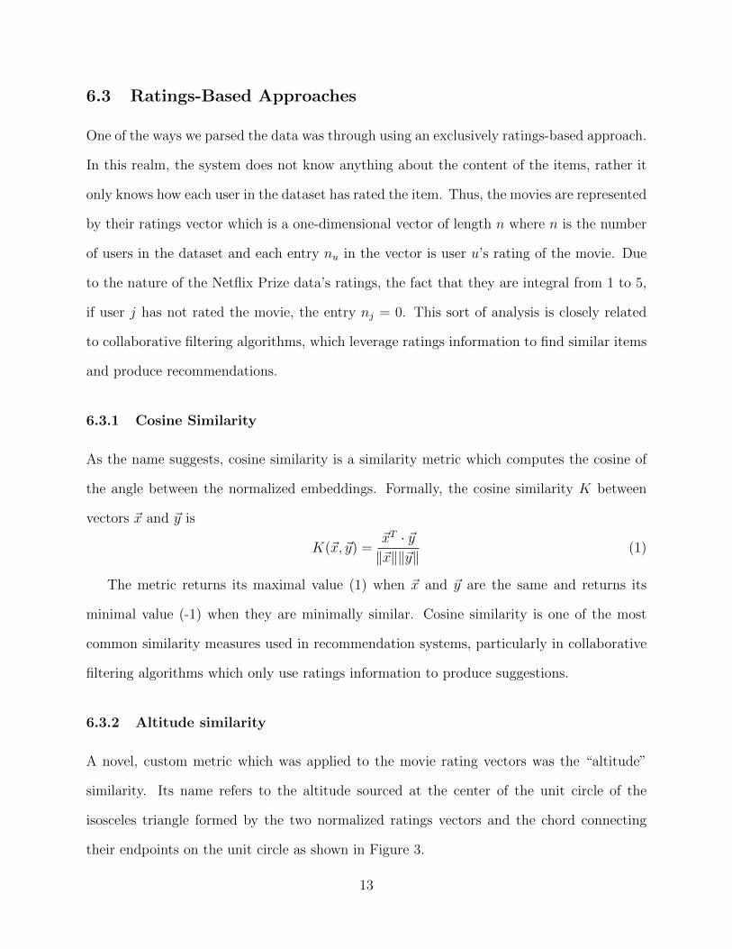
A novel, custom metric which was applied to the movie rating vectors was the “altitude”
similarity. Its name refers to the altitude sourced at the center of the unit circle of the
isosceles triangle formed by the two normalized ratings vectors and the chord connecting
their endpoints on the unit circle as shown in Figure 3.
13

Figure 3: An example of the altitude similarity between two vectors ~CA and ~CB. The
altitude similarity refers to the altitude CD of the triangle4ABC formed by the two vectors
and their chordal distance AB. Note that both vectors are normalized to unit vectors. In
spite of its resemblance to cosine similarity, the altitude similarity produced substantially
different results.
Formally, the altitude similarity A between feature vectors x and y is
A(~x, ~y) = cos
arccos(
~x·~y‖~x‖‖~y‖
)2
(2)
Note that this measure follows all of the properties of a similarity metric. Since it is
bounded by the chord between the endpoints and the center of the unit circle, the range of
the function is [0, 1]. A(~x, ~x) = 1, the maximum of the function, and for two vectors ~u and
~v which are maximally dissimilar to each other, pointing to opposite sides of the unit circle,
A(~u,~v) = 0, the minimum of the function.
6.4 Content-Based Approaches
Another approach we took to analyzing the data was looking at the semantic content of the
movies. This is where the enrichment of the dataset with IMDb came into use. There are
a variety of ways to represent movies given their content: be it the directors, the cast, the
14

genre, the plot of the movies or any combination of them. We chose to use the movie plots
as the basis for our content-based exploration.
6.4.1 Topic Modeling
We chose to use the topic distribution of the movie plots (scraped from IMDb) as the
movie embedding in order to capture the semantic content of the movies. The topics of the
documents were learned via a Latent Dirichlet Allocation (LDA) topic modeling algorithm
[22]. In this context, a topic is a probability distribution over a set of words representing
the likelihood of encountering each word within that topic [23]. The topic model uses word
frequencies to determine the allocation of the words to a topic. Then, every movie summary
can be represented as a distribution of topics [24].
Inspired by [24], several preprocessing steps were taken in order to produce the optimal
topic model. In addition to the traditional steps such as stop-word removal, creating bigrams,
and lemmatizing words, we only chose to analyze documents whose word count was between
50 and 300 in order to guarantee some sort of uniformity in the length of each movie summary.
Furthermore, we removed outlier words from the corpus - specifically, we removed words
which occurred in less than 3 of the documents and those which occurred in more than
20 percent of the documents. To determine the number of topics, we built several models
and compared their CV coherence score to determine which performed the best. The CV
coherence score (i) segments the data into word pairs (ii) calculates word pair probabilities
(iii) calculates a confirmation measure that quantifies how strongly a word set supports
another word set, and finally (iv) aggregates individual confirmation measures into an overall
coherence score [25]. A more comprehensive explanation of the CV coherence measure can
be found in [25]. The highest scoring topic model, and the model with which we represented
the movies, was one with 4 topics and a CV coherence score of 0.417.
To compare the movies with their new embeddings we used the Kullback-Leibler Diver-
15

gence, a dissimilarity measure of their topic distributions described in Section 6.4.2.
To cluster the movies, we wanted to convert the dissimilarity measure into a similarity
measure. There are multiple ways to do this - converting high values to low values - typically
through some strictly decreasing function. We chose to use the Gaussian (also known as RBF
or heat) kernel to convert the metric. That is:
f(xij) = exp−x2ij2σ2
(3)
where xij is the distance between vectors xi and xj (the KL-divergence in this case), and
the “spreading factor” σ is a parameter free for choice to adjust the distribution of the
similarities. The kernel maps the distances onto a bell-curve distribution translating low
values to high ones and high values to low ones. The range of the kernel is (0, 1], and it
is particularly useful in converting distances to similarities because it maps 0 (the minimal
distance) to 1 (the kernel’s maximum value), and it is a one-to-one mapping for positive
values (as distances are).
The parameter σ determines the width of the curve, with higher σ values corresponding
to a wider curve and lower σ values corresponding to a narrower curve. Multiple different σ’s
were explored, with the chosen σ value being that which gave the gave the highest variance in
the new distribution. This was meant to capture the intuition that a similarity distribution
with higher variance would lead to more meaningful clusters. We wanted to spread the
distribution of the similarities out so that we would be able to find the similarities which
were most significant.
6.4.2 Kullback–Leibler Divergence
Kullback-Leibler (KL) divergence, also known as relative entropy, is a common metric for
measuring the difference between probability distributions. Though it is not symmetric, it
is regularly used when comparing two probability distributions, and can be interpreted as
the average difference between the two distributions.
16

Formally, the KL-divergence D of two discrete distributions P and Q in the space X is
D(P || Q) =∑x∈X
P (x) · log
(P (x)
Q(x)
)(4)
To mitigate the issue of symmetry, we used an average of the KL-divergence, so that for two
probability distributions P and Q the KL-divergence was
Dsym(P,Q) =D(P || Q) +D(Q || P )
2(5)
In the context of a topic model, where movies are represented as a vector with their prob-
ability distribution among the various topics, the KL-divergence can be considered a useful
dissimilarity metric between movies. It returns small values when P and Q have similar
distributions and large values when they have dissimilar distributions.
6.5 Hybrid Approaches
The final method of looking at the movies was using a hybrid approach between the ratings
and content based approaches. This was done by defining the similarity between the movies
as a weighted sum between a measure of their ratings vectors and a measure of their proba-
bility distributions. The two metrics we used were the chordal distance between the ratings
vectors (explained in Section 6.5.1) and the KL-divergence of the topic distribution of the
movies (explained in Section 6.4.2) such that the distance between two movies m1 and m2
in this context were
α× dC(m1,m2) + (1− α)×Dsym(m1,m2) (6)
where α ∈ (0, 1), dC(m1,m2) is the chordal distance between movies m1 and m2, and
Dsym(m1,m2) is the symmetric KL-divergence of movies m1 and m2. This weighted method
is one of the most common ways to leverage the power of both content based and ratings
based systems [6].
17
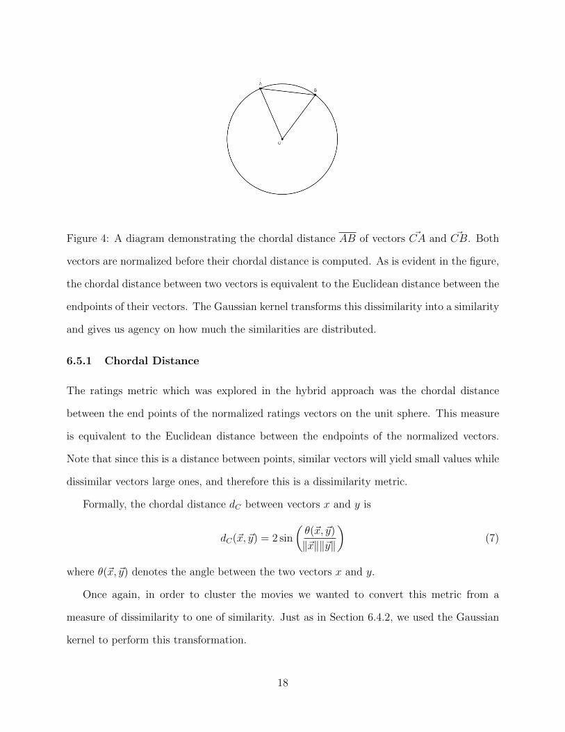
Figure 4: A diagram demonstrating the chordal distance AB of vectors ~CA and ~CB. Both
vectors are normalized before their chordal distance is computed. As is evident in the figure,
the chordal distance between two vectors is equivalent to the Euclidean distance between the
endpoints of their vectors. The Gaussian kernel transforms this dissimilarity into a similarity
and gives us agency on how much the similarities are distributed.
6.5.1 Chordal Distance
The ratings metric which was explored in the hybrid approach was the chordal distance
between the end points of the normalized ratings vectors on the unit sphere. This measure
is equivalent to the Euclidean distance between the endpoints of the normalized vectors.
Note that since this is a distance between points, similar vectors will yield small values while
dissimilar vectors large ones, and therefore this is a dissimilarity metric.
Formally, the chordal distance dC between vectors x and y is
dC(~x, ~y) = 2 sin
(θ(~x, ~y)
‖~x‖‖~y‖
)(7)
where θ(~x, ~y) denotes the angle between the two vectors x and y.
Once again, in order to cluster the movies we wanted to convert this metric from a
measure of dissimilarity to one of similarity. Just as in Section 6.4.2, we used the Gaussian
kernel to perform this transformation.
18

6.6 Graph Sparsification
Algorithm 2 Locally Adaptive Network Sparsification (W,α)
1: Compute the fractional edge weight pij between all pairs of nodes i, j where
pij =wij∑Ni
k=1wik
where Ni denotes the neighborhood or degree of node i.2: For each edge, get the fraction of edges sourced at node i which have a fractional edge
weight less than the edge in question. That is, for each node i and each neighbor j,calculate
F (pij) =1
Ni
Ni∑k=1
1{pik < pij}
3: Construct W ′ ∈ Rn×n where W ′(i, j) = W (i, j) if and only if 1 − F (pij) < α and 0otherwise.
4: return the new weighted adjacency matrix W ′.
Graph sparsification is the process of removing edges from a graph or network in order to
reveal some underlying network structure. This is especially useful in the context of dense
network study where there can be too many edges to perform any meaningful analysis. The
sparsification is typically done by applying a global threshold wherein all edges which meet
or exceed the threshold will be retained in the sparsified graph. This approach is inadequate
when applied to “real-world” data, where the similarity among the data is highly unevenly
distributed [19, 26, 27]. A more promising manner is to consider edges which are locally
significant and keep only those which meet this criteria.
The sparsification approach which was applied to the visualizations was first proposed
by [19] and is called locally adaptive network sparsification (LANS). The method can be
applied to any sort of similarity matrix, independent of its distribution, and has been shown
to be effective in pulling meaningful backbones out of networks where fractional edge weight
distributions are highly heterogeneous [19].
The algorithm takes as input the weighted adjacency matrix W ∈ Rn×n where n is the
number of nodes in the graph and a significance level α ∈ [0, 1]. We use the notation wij
19

to denote the weight of the edge between node i and j. The procedure for this algorithm is
described in Algorithm 2.
7 Evaluation
We evaluated the performance of each approach on the homogeneity of the genres in the
clusters which the spectral clustering algorithm was able to find. If the approach performed
well, it should be able to find the most significant similarities between items which do have
some sort of “ground truth” similarity between them. We chose to use the genre labels
scraped from IMDb as our “ground truth” notion of similarity. These genres were:
1. Action
2. Adventure
3. Animation
4. Biography
5. Comedy
6. Crime
7. Documentary
8. Drama
9. Family
10. Fantasy
11. Film-Noir
12. Game-Show
13. History
14. Horror
15. Music
16. Musical
17. Mystery
18. News
19. Reality-TV
20. Romance
21. Sci-Fi
22. Short
23. Sport
24. Talk-Show
25. Thriller
26. War
27. Western
To measurably assess the success of the clusters, we developed a customized homogeneity
score which would be more flexible than the traditional approach for the purpose of taking
into account the multiple labels which the data had [28]. As is notable from the list above,
there may be movies which are similar to each other on the basis of genre that may take
multiple genre labels to be realized. For example, a movie which is a romantic comedy and
a movie which is a family comedy may not be understood by the computer to be similar
if only looking at the first genre. Even more obvious, a movie which is a romantic comedy
20

and a movie which is a comedic romance may run into the same issue. Thus, we opted to
develop a metric which would mitigate this issue.
7.1 Customized Homogeneity Metric
The score is an analysis of how homogeneous the produced clusters were in terms of the first
n genre tags of each movie. For each cluster, the metric computes the most common genre
tag in the first n tags of each movie in the cluster and finds the proportion of movies in the
cluster which have that genre tag (this is the homogeneity of a cluster). It finds the average
homogeneity among all of the clusters as its final value. Note that this metric is in the range
[0, 1], where 1 implies a perfectly homogeneous clustering among all of the clusters found
and 0 implies a completely heterogeneous clustering. As n increases, the metric gravitates
towards higher values as there are more genres considered for the possibility of a match.
Additionally, the metric is biased towards a larger number of clusters: imagine a clustering
where each movie belongs to its own cluster. Thus, the metric is likely to tend to give
values closer to 1 than to 0, and it is best used when comparing different clusterings to each
other as opposed to different clusterings relative to the ground truth labelling. Formally, the
customized homogeneity metric hn of labels C and G is:
hn(C,G) =∑Ci∈C
# of movies in Ci with label gi| Ci |
(8)
where C is the set of clusters, G the ground truth labeling, n is the number of genre tags to
consider, and gi is the most common label in G of the items in Ci. In this context, gi is the
most frequently occurring genre tag in the first n genre tags of the movies in cluster Ci.
8 Results
For each experiment we carried out, each approach we tried on the various subsets of the data,
we tested the performance of the clusters across a range of different numbers of clusters. We
21

compared our customized homogeneity score to analyze how well the different approaches
worked on the subsets of the data. We computed the average homogeneity score for the
different metrics and subsets across a range of 4 clusters to 24 clusters. A common way
to determine the number of clusters to produce in spectral clustering is to plot the sorted
eigenvalues of the similarity matrix and find the elbow of the curve [21]. The k at which
the curve begins to bend is typically chosen as the number of clusters to produce. For the
similarity matrices with which we dealt, this k was regularly between 10 and 18, so we chose
the numbers 4 and 24 in order to explore different places along the curve to set k while
ensuring that reasonable k’s would be within range to find reasonably sized clusters. When
comparing the different methods, we took the difference in the homogeneity at each distinct
clustering between the methods and then took the average of the differences. That is, for
each subset, we took the difference between the scores for two metrics at 4 clusters, 6 clusters,
and so on, and then took the average of the differences to evaluate their performances relative
each other.
Figures 5, 6, 7 show the results of each approach on the most popular movies, the least
popular movies, and the top and bottom composite respectively. The following sections focus
on the results within the context of the different approaches considered.
8.1 Ratings-Based Results
Within the ratings based approach, we explored two different similarity metrics, cosine sim-
ilarity and altitude similarity.
We found that altitude similarity and cosine similarity performed relatively similarly in
the most popular movies. In particular, in the most popular subset, the clusters produced
with altitude similarity scored an average of 0.044 better on h2 and 0.045 better on h3 than
those found with cosine similarity. There was a much greater difference in performance in
the top and bottom and the lightly reviewed subsets. On average, in the top and bottom
22

Figure 5: Average homogeneity of the clusters of each approach on the most popular 2000
movies in the dataset. We chose to show the best performing hybrid model in the figure.
For this subset, this was the hybrid system with α = 0.75 - weighing more heavily on the
ratings.
subset altitude similarity’s clusters scored 0.085 higher on h2 and 0.084 higher on h3. In
contrast, cosine similarity vastly outperformed altitude similarity in the context of finding
homogeneous clusters in the least popular subset. In particular, cosine similarity was able
to find clusters which were on average 0.13 higher on h2 and 0.15 higher on h3.
These results suggest that altitude similarity could be a promising metric for bridging the
gap between the most and least popular movies, bringing lightly reviewed movies to the eyes
of the customer, particularly in a collaborative filtering system. However, once restricting the
scope of the data to the lightly reviewed items, cosine similarity provides more meaningful
similarity measures between lightly reviewed movies.
8.2 Comparing Ratings-Based and Content-Based Results
We compared the homogeneity of the clusters found with the content-based, topic model
approach to the best clusters in each subset with the ratings based approach, where best is
defined as having the highest homogeneity score. Thus, for the most popular subset and the
23
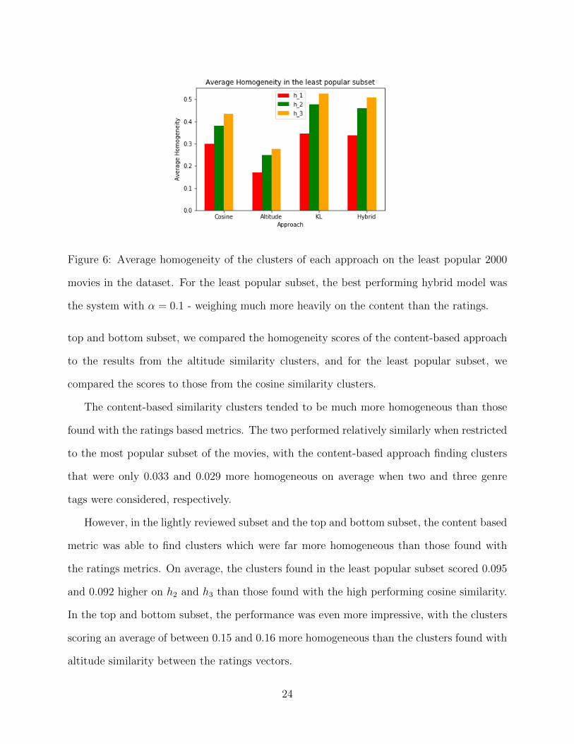
Figure 6: Average homogeneity of the clusters of each approach on the least popular 2000
movies in the dataset. For the least popular subset, the best performing hybrid model was
the system with α = 0.1 - weighing much more heavily on the content than the ratings.
top and bottom subset, we compared the homogeneity scores of the content-based approach
to the results from the altitude similarity clusters, and for the least popular subset, we
compared the scores to those from the cosine similarity clusters.
The content-based similarity clusters tended to be much more homogeneous than those
found with the ratings based metrics. The two performed relatively similarly when restricted
to the most popular subset of the movies, with the content-based approach finding clusters
that were only 0.033 and 0.029 more homogeneous on average when two and three genre
tags were considered, respectively.
However, in the lightly reviewed subset and the top and bottom subset, the content based
metric was able to find clusters which were far more homogeneous than those found with
the ratings metrics. On average, the clusters found in the least popular subset scored 0.095
and 0.092 higher on h2 and h3 than those found with the high performing cosine similarity.
In the top and bottom subset, the performance was even more impressive, with the clusters
scoring an average of between 0.15 and 0.16 more homogeneous than the clusters found with
altitude similarity between the ratings vectors.
24

Figure 7: Average homogeneity of the clusters of each approach on the most popular 1000
movies and the least popular 1000 movies in the dataset. The hybrid model in this figure is
the one with α = 0.66.
The results are certainly impressive, however they are not necessarily surprising given our
metric for evaluation. Since we are assessing the clusters on the homogeneity of the genre
tags, it should follow that a content-based approach which takes into account the movies’
topics will result in clusters with many similar genres - which are themselves a part of the
movies’ content. Nevertheless, it is undoubtedly noteworthy that the content based approach
was able to outperform the ratings based approach in almost every way.
8.3 Hybrid Results
Since the content-based approach outperformed the ratings-based approach on every subset
of the data which we analyzed, we used the content-based approach as a benchmark to
evaluate the performance of our hybrid methods. On the most popular subset, the hybrid
methods showed a promising improvement in performance. We created three different hybrid
systems, one with α = 0.25, one with α = 0.50, and one with α = 0.75. The best performance
came from those which relied more heavily on the ratings data than the plot summaries,
namely the model with α = 0.5 and the model with α = 0.75. This was an unexpected
25

result, since the strictly content-based approach had outperformed the strictly ratings-based
approach. However, when both of the metrics came together, they were able to find clusters
which scored 0.053 and 0.072 higher on h2 and h3, respectively.
In the least popular subset, we found that weighing the topic model more heavily was
advantageous. This was consistent with the results we had obtained when comparing the
previous approaches. We evaluated multiple α values, but none of them were able to outper-
form the strictly content-based approach. The closest match to the content-based filtering
approach was a hybrid system with α = 0.1, relying very heavily on the content-based ap-
proach, which was the smallest α we were willing to consider before losing the complexity of
a hybrid approach. This metric only scored 0.016 and 0.017 lower on h2 and h3, respectively,
than the strictly content-based approach.
Finally, in the top and bottom subset, we found that giving more weight to the ratings
information produced better results. We tested the system at multiple different α values
and saw the greatest jump in performance with α = 0.66. This gave clusters which were
0.051 more homogeneous on 2 genre tags and 0.067 more homogeneous with 3 genre tags
on average. Interestingly, the performance did not necessarily improve as α increased. For
instance, the system with α = 0.8 saw clusters which were on average only 0.044 and 0.053
more homogeneous on 2 and 3 genre tags, respectively.
9 Conclusion
We have performed a survey of what sorts of approaches and what sorts of metrics work
best on different areas of the Netflix Prize data. We evaluate the performance of a metric
by the homogeneity of genres in the clusters which are produced through applying spectral
clustering to the various similarity matrices.
We find that the novel altitude similarity can outperform the more traditional cosine sim-
ilarity in the context of the most popular movies and the top/bottom composite subset, while
26
cosine similarity reigns superior in the least popular subset. The content-based approach
outperforms the ratings-based approach in all subsets and all measures of homogeneity. In
spite of this, in the most popular subset of movies, a hybrid system with a greater emphasis
on the ratings information is able to find the most homogeneous clusters. Similarly, in the
top and bottom composite subset, a hybrid system which leans heavily on ratings - though
not as much as the system in the most popular subset - is most successful at finding uniform
clusters. In the least popular subset, no approach beats the strictly content-based approach
built on the topic distribution of the movies.
The results suggest that a recommendation system which aims for the ability to make
meaningful, sensible recommendations on the least popular items in its catalog should use a
ratings-heavy hybrid approach to connect the head and tail of the dataset, and then move to
using strictly content based system (or a content-heavy hybrid system) to make suggestions
between items in the tail.
10 Future Work
There are many possible areas to go forward from the survey of different approaches accom-
plished in this paper. Firstly, doing a similar experiment with the inclusion of a random
subset of the items would be helpful in determining whether the approaches can be applica-
ble to a portion of the data which has less in common. We evaluated the performance of our
approaches on the homogeneity of the genres found in the clusters which were produced from
the similarity metrics we used. While useful, this is different than evaluating the relevance
of our approaches on suggestions a system may make. Therefore, a useful direction to take
the project would be to apply some of the metrics proposed in [29, 30] to evaluate the per-
formance of the different approaches presented in this paper. This analysis would produce a
better understanding of the applicability of these approaches to full-fledged recommendation
engines.
27

Another direction to take the project would be to create a visual representation of the
similarities between the different movies based on the different approaches. This would
build on the work done in [31, 32, 33, 23] where visual tools are created to demonstrate the
relationship between items. In [32, 33, 23] in particular, a sense of geometry and direction
within the network is explored. This would be particularly be effective in the long tail of
the data where users may be lost regarding the association of different items. Users would
be able to traverse the “terrain” of movies and gain a better understanding of where their
preferred movies fit within the space, and where moving in different directions from a seeded
movie will take them. It would even be interesting for users to investigate what the “path”
between two movies looks like when considering different similarity metrics.
Lastly, this survey of approaches could be applied to another itemset. A similar analysis
on a different itemset would give a better understanding of where each sort of approach is
most effective. A library’s inventory may be a great next itemset to work with given the
similarity between books and movies. In both cases, the items can be represented by their
ratings, their semantic content, or their genres.
Acknowledgments
I would first like to thank my advisor, Professor Daniel Rockmore, for his guidance, support,
and patience throughout this project. Additionally, I would like to acknowledge and thank
Professor Allen Riddell for his assistance and input with the project, and Tommaso Carraro
for his cooperation in helping me combine the Netflix and IMDb datasets. I would like to
thank Dartmouth College for giving me the opportunity to pursue a thesis.
I would like to thank my friends and my family who supported me as I worked on this
study. Lastly, I want to extend my gratitude to the engineers who worked on the following
technologies which I used in my analysis: [34, 35, 22, 36, 37, 38].
28

References
[1] C. Anderson and M. P. Andersson, “Long tail,” 2004.
[2] H. Yin, B. Cui, J. Li, J. Yao, and C. Chen, “Challenging the Long Tail Recommenda-
tion,” arXiv:1205.6700 [cs], May 2012. arXiv: 1205.6700.
[3] B. Hallinan and T. Striphas, “Recommended for you: The Netflix Prize and the pro-
duction of algorithmic culture - Blake Hallinan, Ted Striphas, 2016.”
[4] M. Balabanovic and Y. Shoham, “Fab: content-based, collaborative recommendation,”
Communications of the ACM, vol. 40, pp. 66–72, Mar. 1997.
[5] R. Van Meteren and M. Van Someren, “Using content-based filtering for recommen-
dation,” in Proceedings of the machine learning in the new information age: ML-
net/ECML2000 workshop, vol. 30, pp. 47–56, 2000.
[6] G. Lekakos and P. Caravelas, “A hybrid approach for movie recommendation,” Multi-
media Tools and Applications, vol. 36, pp. 55–70, Jan. 2008.
[7] M. J. Pazzani and D. Billsus, “Content-Based Recommendation Systems,” in The Adap-
tive Web: Methods and Strategies of Web Personalization (P. Brusilovsky, A. Kobsa, and
W. Nejdl, eds.), Lecture Notes in Computer Science, pp. 325–341, Berlin, Heidelberg:
Springer, 2007.
[8] J. L. Herlocker, J. A. Konstan, and J. Riedl, “Explaining collaborative filtering rec-
ommendations,” in Proceedings of the 2000 ACM conference on Computer supported
cooperative work, CSCW ’00, (New York, NY, USA), pp. 241–250, Association for Com-
puting Machinery, Dec. 2000.
[9] A. Mnih and R. R. Salakhutdinov, “Probabilistic matrix factorization,” Advances in
neural information processing systems, vol. 20, pp. 1257–1264, 2007.
29

[10] Y. Koren, R. Bell, and C. Volinsky, “Matrix Factorization Techniques for Recommender
Systems,” Computer, vol. 42, pp. 30–37, Aug. 2009. Conference Name: Computer.
[11] J. B. Schafer, D. Frankowski, J. Herlocker, and S. Sen, “Collaborative Filtering Recom-
mender Systems,” in The Adaptive Web: Methods and Strategies of Web Personalization
(P. Brusilovsky, A. Kobsa, and W. Nejdl, eds.), Lecture Notes in Computer Science,
pp. 291–324, Berlin, Heidelberg: Springer, 2007.
[12] G. Adomavicius and A. Tuzhilin, “Toward the next generation of recommender sys-
tems: a survey of the state-of-the-art and possible extensions,” IEEE Transactions on
Knowledge and Data Engineering, vol. 17, pp. 734–749, June 2005. Conference Name:
IEEE Transactions on Knowledge and Data Engineering.
[13] M.-L. Wu, C.-H. Chang, and R.-Z. Liu, “Integrating content-based filtering with col-
laborative filtering using co-clustering with augmented matrices,” Expert Systems with
Applications, vol. 41, pp. 2754–2761, May 2014.
[14] J. Li, K. Lu, Z. Huang, and H. T. Shen, “Two Birds One Stone: On both Cold-Start and
Long-Tail Recommendation,” in Proceedings of the 25th ACM international conference
on Multimedia, MM ’17, (New York, NY, USA), pp. 898–906, Association for Computing
Machinery, Oct. 2017.
[15] M. Levy and K. Bosteels, “Music recommendation and the long tail,” in 1st Work-
shop On Music Recommendation And Discovery (WOMRAD), ACM RecSys, 2010,
Barcelona, Spain, Citeseer, 2010.
[16] H. Yang, “Targeted search and the long tail effect,” The RAND
Journal of Economics, vol. 44, no. 4, pp. 733–756, 2013. eprint:
https://onlinelibrary.wiley.com/doi/pdf/10.1111/1756-2171.12036.
30
[17] J. Bennett, S. Lanning, and N. Netflix, “The Netflix Prize,” in In KDD Cup and Work-
shop in conjunction with KDD, 2007.
[18] N. Bhatia and P. Patnaik, “Netflix recommendation based on imdb,” 2008.
[19] N. J. Foti, J. M. Hughes, and D. N. Rockmore, “Nonparametric Sparsification of Com-
plex Multiscale Networks,” PLOS ONE, vol. 6, p. e16431, Feb. 2011. Publisher: Public
Library of Science.
[20] J. Shi and J. Malik, “Normalized cuts and image segmentation,” IEEE Transactions on
Pattern Analysis and Machine Intelligence, vol. 22, pp. 888–905, Aug. 2000. Conference
Name: IEEE Transactions on Pattern Analysis and Machine Intelligence.
[21] U. von Luxburg, “A tutorial on spectral clustering,” Statistics and Computing, vol. 17,
pp. 395–416, Dec. 2007.
[22] R. Rehurek and P. Sojka, “Software Framework for Topic Modelling with Large Cor-
pora,” in Proceedings of the LREC 2010 Workshop on New Challenges for NLP Frame-
works, (Valletta, Malta), pp. 45–50, ELRA, May 2010.
[23] R. Blankemeier, “Information Network Navigation,” Dartmouth College Undergraduate
Theses, June 2020.
[24] M. Saxton, “A Gentle Introduction to Topic Modeling Using Python,” Theological Li-
brarianship, vol. 11, pp. 18–27, Apr. 2018.
[25] S. Syed and M. Spruit, “Full-Text or Abstract? Examining Topic Coherence Scores
Using Latent Dirichlet Allocation,” in 2017 IEEE International Conference on Data
Science and Advanced Analytics (DSAA), pp. 165–174, Oct. 2017.
31
[26] P. B. Slater, “Multiscale Network Reduction Methodologies: Bistochastic and Disparity
Filtering of Human Migration Flows between 3,000+ U. S. Counties,” arXiv:0907.2393
[physics, stat], Sept. 2010. arXiv: 0907.2393.
[27] M. A. Serrano, M. Boguna, and A. Vespignani, “Extracting the multiscale backbone of
complex weighted networks,” Proceedings of the National Academy of Sciences, vol. 106,
pp. 6483–6488, Apr. 2009. arXiv: 0904.2389.
[28] A. Rosenberg and J. Hirschberg, “V-Measure: A Conditional Entropy-Based External
Cluster Evaluation Measure,” in Proceedings of the 2007 Joint Conference on Empirical
Methods in Natural Language Processing and Computational Natural Language Learning
(EMNLP-CoNLL), (Prague, Czech Republic), pp. 410–420, Association for Computa-
tional Linguistics, June 2007.
[29] S. Vargas and P. Castells, “Rank and relevance in novelty and diversity metrics for
recommender systems,” in Proceedings of the fifth ACM conference on Recommender
systems, RecSys ’11, (New York, NY, USA), pp. 109–116, Association for Computing
Machinery, Oct. 2011.
[30] Y. Shi, A. Karatzoglou, L. Baltrunas, M. Larson, A. Hanjalic, and N. Oliver, “TFMAP:
optimizing MAP for top-n context-aware recommendation,” in Proceedings of the 35th
international ACM SIGIR conference on Research and development in information re-
trieval - SIGIR ’12, (Portland, Oregon, USA), p. 155, ACM Press, 2012.
[31] K. Wegba, A. Lu, Y. Li, and W. Wang, “Interactive Storytelling for Movie Recom-
mendation through Latent Semantic Analysis,” in 23rd International Conference on
Intelligent User Interfaces, IUI ’18, (New York, NY, USA), pp. 521–533, Association
for Computing Machinery, Mar. 2018.
32

[32] G. Leibon and D. N. Rockmore, “Orienteering in Knowledge Spaces: The Hyperbolic
Geometry of Wikipedia Mathematics,” PLOS ONE, vol. 8, p. e67508, July 2013. Pub-
lisher: Public Library of Science.
[33] C. An and D. N. Rockmore, “Open Personalized Navigation on the Sandbox of Wiki
Pages,” in Companion Proceedings of The 2019 World Wide Web Conference, WWW
’19, (New York, NY, USA), pp. 1173–1179, Association for Computing Machinery, May
2019.
[34] P. Virtanen, R. Gommers, T. E. Oliphant, M. Haberland, T. Reddy, D. Cournapeau,
E. Burovski, P. Peterson, W. Weckesser, J. Bright, S. J. van der Walt, M. Brett, J. Wil-
son, K. J. Millman, N. Mayorov, A. R. J. Nelson, E. Jones, R. Kern, E. Larson, C. J.
Carey, I. Polat, Y. Feng, E. W. Moore, J. VanderPlas, D. Laxalde, J. Perktold, R. Cim-
rman, I. Henriksen, E. A. Quintero, C. R. Harris, A. M. Archibald, A. H. Ribeiro,
F. Pedregosa, P. van Mulbregt, and SciPy 1.0 Contributors, “SciPy 1.0: Fundamental
Algorithms for Scientific Computing in Python,” Nature Methods, vol. 17, pp. 261–272,
2020.
[35] F. Pedregosa, G. Varoquaux, A. Gramfort, V. Michel, B. Thirion, O. Grisel, M. Blondel,
P. Prettenhofer, R. Weiss, V. Dubourg, J. Vanderplas, A. Passos, D. Cournapeau,
M. Brucher, M. Perrot, and E. Duchesnay, “Scikit-learn: Machine learning in Python,”
Journal of Machine Learning Research, vol. 12, pp. 2825–2830, 2011.
[36] J. D. Hunter, “Matplotlib: A 2d graphics environment,” Computing in Science & En-
gineering, vol. 9, no. 3, pp. 90–95, 2007.
[37] C. R. Harris, K. J. Millman, S. J. van der Walt, R. Gommers, P. Virtanen, D. Courna-
peau, E. Wieser, J. Taylor, S. Berg, N. J. Smith, R. Kern, M. Picus, S. Hoyer, M. H.
van Kerkwijk, M. Brett, A. Haldane, J. F. del Rıo, M. Wiebe, P. Peterson, P. Gerard-
Marchant, K. Sheppard, T. Reddy, W. Weckesser, H. Abbasi, C. Gohlke, and T. E.
33

Oliphant, “Array programming with NumPy,” Nature, vol. 585, pp. 357–362, Sept.
2020.
[38] Wes McKinney, “Data Structures for Statistical Computing in Python,” in Proceedings
of the 9th Python in Science Conference (Stefan van der Walt and Jarrod Millman,
eds.), pp. 56 – 61, 2010.
34

A Graph Visualizations
Figure 8: These are all networks formed with the top and bottom 1,000 movies. Clockwise
from the top left: the altitude similarity network, the cosine similarity network, the entropy
network, and the hybrid metric with α = 0.66. The graphs are colored by popularity, where
green implies a movie belongs to the most popular 1,000 movies and pink implies a movie
belongs to the least popular 1,000 movies. The altitude similarity and cosine similarity
networks are shown with a LANS threshold of 0.002, while the entropy and hybrid networks
have a LANS threshold of 0.006.
35

Figure 9: These are some of the networks formed with the most popular subset of the data.
Clockwise from the left, the altitude similarity network, the cosine similarity network, and
the entropy network. The graphs are colored based on the clusters found in the spectral
clustering algorithm, with each graph having 18 clusters. The cosine and altitude similarity
graphs are shown with a LANS threshold of 0.001, while the entropy graph has a LANS
threshold of 0.003.
Figure 10: These are some of the networks formed with the least popular subset of the data.
As is evident, the lack of information in this subset results in poorer clustering. Clockwise
from the left, the altitude similarity network, the cosine similarity network, and the entropy
network. The graphs are colored based on the clusters found in the spectral clustering
algorithm, with each graph again having 18 clusters. The cosine and altitude similarity
graphs are shown with a LANS threshold of 0.001, while the entropy graph has a LANS
threshold of 0.003.
36
Related Documents