Exploring generative adversarial networks for controllable ...

HAL Id: tel-03640610https://tel.archives-ouvertes.fr/tel-03640610

Submitted on 13 Apr 2022

HAL is a multi-disciplinary open accessarchive for the deposit and dissemination of sci-entific research documents, whether they are pub-lished or not. The documents may come fromteaching and research institutions in France orabroad, or from public or private research centers.

L’archive ouverte pluridisciplinaire HAL, estdestinée au dépôt et à la diffusion de documentsscientifiques de niveau recherche, publiés ou non,émanant des établissements d’enseignement et derecherche français ou étrangers, des laboratoirespublics ou privés.

Exploring generative adversarial networks forcontrollable musical audio synthesis

Javier Nistal Hurle

To cite this version:Javier Nistal Hurle. Exploring generative adversarial networks for controllable musical audio synthesis.Sound [cs.SD]. Institut Polytechnique de Paris, 2022. English. �NNT : 2022IPPAT009�. �tel-03640610�

626

NN

T:2

022I

PPA

T009 Exploring Generative Adversarial

Networks for Controllable Musical AudioSynthesis

These de doctorat de l’Institut Polytechnique de Parispreparee a Telecom Paris

Ecole doctorale n◦626 Institut Polytechnique de Paris (EDIPP)Specialite de doctorat : Signal, Images, Automatique et robotique

These presentee et soutenue a Palaiseau, le 9/03/2022, par

JAVIER NISTAL HURLE

Composition du Jury :

Axel RoebelResearch Director, IRCAM (SAS), Paris, France President

Xavier SerraProfessor, Universitat Pompeu Fabra (MTG), Barcelona, Spain Rapporteur

Sølvi YstadResearch Director, CNRS (PRISM), Marseille, France Rapporteuse

Mathieu FontaineAssociate Professor, Telecom Paris, IP Paris, France Examinateur

Gael RichardProfessor, Telecom Paris, IP Paris, France Directeur de these

Stefan LattnerAssociate Researcher, Sony CSL, Paris, France Co-directeur de these

Lonce WyseAssociate Professor, NUS (CNM), Singapore Invite

Jean-Baptiste RollandResearch Senior Software Developer, Steinberg MediaTechnologies, Germany Invite

2

Acknowledgement

First and foremost, I am extremely grateful to my supervisors, Prof. Gaël Richardand Dr. Stefan Lattner, for counting on me for this project and their invaluableadvice, continuous support, and patience during my Ph.D. study. Their immenseknowledge and plentiful experience have encouraged me in all the time of my aca-demic research and daily life. I would especially like to appreciate the implicationof Stefan in any hurdle along the way of this project, you name it: writing, cod-ing, inspiration, bureaucracy, existential... Stefan has spent very long deadlinenights and has been there for any problem I could have. I would like to speciallymention our late-night inspirational discussions at Outland bar, resulting in mostof the crazy ideas behind the work described here and many others to be carriedout. I’m looking forward to our future projects.

I want to thank all the staff at Sony CSL for making this Ph.D. projectpossible. It is their kind help and support that have made my study and life inParis a wonderful time. I would like to send a special thanks to some colleaguesand former colleagues:

• Emmanuel Deruty, for supporting my work and providing unlimited re-sources to make it possible (e.g., data, GPUs, promotion). The impact,reach, and, ultimately, the success of this project has significantly beenpossible thanks to his work. I would also like to appreciate his trust andconfidence in my work and autonomy.

• Cyran Aouameur, for his fellowship and continuous support, in and outsidethe lab. Cyran created DrumGAN’s VST interface and has continuouslysupported me with any matter (e.g., writing, presentations, coding, bureau-cracy, well-being). It’s been an absolute pleasure working with him, and Ihope we’ll continue doing so for long!

• Michael Turbot, for his implication and confidence in my work, and specif-ically in DrumGAN. He was responsible for creating a promotional videoteaser about my work, and he has contributed to the reach and impact ofthis project.

• Michael Anslow, for his friendship and support and, also, our many inspi-rational conversations.

• Dr. Gaëtan Hadjeres, Dr. Leopold Crestel, Dr. Maarten Grachten, andTheis Bazin for their always thoughtful input and support and for theirwork’s inspiration.

• Dr. Matthias Demoucron, for his implication in DrumGAN and his supportwith many legal and bureaucratic issues.

3

• Amaury Delourt, for helping me with any data-related matter, and hisinterest in my work.

• Pratik Bhoir, for his patience and support with any IT matter. Thanks tohim, connecting to servers, using Sony’s internal services, and configuringmy computer has been a piece of cake.

• Dr. Stephane Rivaud, for his excellent lectures on GANs and the inspira-tional talks at the beginning of my Ph.D.

• Ithan Velarde, for his work on DrumGAN’s encoder.

• Jeremy Uzan, for his interest in my work and his support outside the lab.

• Sophie Boucher and Cristina Nunu, for supporting and helping me with anybureaucratic and legal issues I could have.

I would like to thank all the members of the ADASP group at Telecom andthe MIP-Frontiers network. I would like to specially thank my colleagues GiorgiaCantisani, Karim Ibrahim, Kilian Schultz, and Ondrej Cifka for their supportthroughout the project.

Finally, I would like to express my gratitude to my parents, my brother andmy friends. Without their tremendous understanding and encouragement in thepast three years, it would have been impossible for me to complete this work inone piece.

This work was supported by the European Union’s Horizon 2020 research andinnovation programme under the Marie Skłodowska-Curie grant agreement No.765068 (MIP-Frontiers).

4

Abstract

Audio synthesizers are electronic musical instruments that generate artificialsounds under some parametric control. While synthesizers have evolved sincethey were popularized in the 70s, two fundamental challenges are still unresolved:1) the development of synthesis systems responding to semantically intuitive pa-rameters; 2) the design of "universal," source-agnostic synthesis techniques. Thisthesis researches the use of Generative Adversarial Networks (GAN) towardsbuilding such systems. The main goal is to research and develop novel toolsfor music production that afford intuitive and expressive means of sound manip-ulation, e.g., by controlling parameters that respond to perceptual properties ofthe sound and other high-level features.

Our first work studies the performance of GANs when trained on variouscommon audio signal representations (e.g., waveform, time-frequency representa-tions). These experiments compare different forms of audio data in the contextof tonal sound synthesis. Results show that the Magnitude and InstantaneousFrequency of the phase and the complex-valued Short-Time Fourier Transformachieve the best results.

Building on this, our following work presents DrumGAN, a controllable ad-versarial audio synthesizer of percussive sounds. We demonstrate that intuitivecontrol can be gained over the generation process by conditioning the model onperceptual features describing high-level timbre properties. This work results indeveloping a VST plugin generating full-resolution audio and compatible with anyDigital Audio Workstation (DAW). We show extensive musical material producedby professional artists from Sony ATV using DrumGAN.

The scarcity of annotations in musical audio datasets challenges the appli-cation of supervised methods to conditional generation settings. Our third con-tribution employs a knowledge distillation approach to extract such annotationsfrom a pre-trained audio tagging system. DarkGAN is an adversarial synthe-sizer of tonal sounds that employs the output probabilities of such a system (so-called “soft labels”) as conditional information. Results show that DarkGAN canrespond moderately to many intuitive attributes, even with out-of-distributioninput conditioning.

Applications of GANs to audio synthesis typically learn from fixed-size two-dimensional spectrogram data analogously to the "image data" in computer vi-sion; thus, they cannot generate sounds with variable duration. Our fourth paperaddresses this limitation by exploiting a self-supervised method for learning dis-crete features from sequential data. Such features are used as conditional input toprovide step-wise time-dependent information to the model. Global consistencyis ensured by fixing the input noise z (characteristic in adversarial settings). Re-sults show that, while models trained on a fixed-size scheme obtain better audio

5

quality and diversity, ours can competently generate audio of any duration.One interesting direction for research is the generation of audio conditioned

on preexisting musical material, e.g., the generation of some drum pattern giventhe recording of a bass line. Our fifth paper explores a simple pretext tasktailored at learning such types of complex musical relationships. Concretely, westudy whether a GAN generator, conditioned on highly compressed MP3 musicalaudio signals, can generate outputs resembling the original uncompressed audio.Results show that the GAN can improve the quality of the audio signals over theMP3 versions for very high compression rates (16 and 32 kbit/s).

As a direct consequence of applying artificial intelligence techniques in mu-sical contexts, we ask how AI-based technology can foster innovation in musicalpractice. Therefore, we conclude this thesis by providing a broad perspectiveon the development of AI tools for music production, informed by theoreticalconsiderations and reports from real-world AI tool usage by professional artists.

6

Résumé

Les synthétiseurs audio sont des instruments de musique électroniques qui génèrentdes sons artificiels sous un certain contrôle paramétrique. Alors que les synthé-tiseurs ont évolué depuis leur popularisation dans les années 70, deux défis fonda-mentaux restent encore non résolus: 1) le développement de systèmes de synthèserépondant à des paramètres sémantiquement intuitifs; 2) la conception de tech-niques de synthèse «universelles», indépendantes de la source à modéliser. Cettethèse étudie l’utilisation des réseaux adversariaux génératifs (ou GAN) pour con-struire de tels systèmes. L’objectif principal est de rechercher et de développerde nouveaux outils pour la production musicale, qui offrent des moyens intuitifset expressifs de manipulation du son, par exemple en contrôlant des paramètresqui répondent aux propriétés perceptives du son et à d’autres caractéristiques.

Notre premier travail étudie les performances des GAN lorsqu’ils sont en-traînés sur diverses représentations de signaux audio (par exemple, forme d’onde,représentations temps-fréquence). Ces expériences comparent différentes formesde données audio dans le contexte de la synthèse sonore tonale. Les résultats mon-trent que la représentation magnitude-fréquence instantanée et la transformée deFourier à valeur complexe obtiennent les meilleurs résultats.

En s’appuyant sur ce résultat, notre travail suivant présente DrumGAN, unsynthétiseur audio de sons percussifs. En conditionnant le modèle sur des car-actéristiques perceptives décrivant des propriétés timbrales de haut niveau, nousdémontrons qu’un contrôle intuitif peut être obtenu sur le processus de génération.Ce travail aboutit au développement d’un plugin VST générant de l’audio hauterésolution et compatible avec les Stations de Travail Audio Numériques (STAN).Nous montrons un vaste matériel musical produit par des artistes professionnelsde Sony ATV à l’aide de DrumGAN.

La rareté des annotations dans les ensembles de données audio musicales remeten cause l’application de méthodes supervisées pour la génération conditionnelle.Notre troisième contribution utilise une approche de distillation des connaissancespour extraire de telles annotations à partir d’un système d’étiquetage audio pré-entraîné. DarkGAN est un synthétiseur de sons tonaux qui utilise les probabilitésde sortie d’un tel système (appelées « étiquettes souples ») comme informationsconditionnelles. Les résultats montrent que DarkGAN peut répondre modérémentà de nombreux attributs intuitifs, même avec un conditionnement d’entrée horsdistribution.

Les applications des GAN à la synthèse audio apprennent généralement à par-tir de données de spectrogramme de taille fixe, de manière analogue aux «donnéesd’image» en vision par ordinateur; ainsi, ils ne peuvent pas générer de sons dedurée variable. Dans notre quatrième article, nous abordons cette limitation enexploitant une méthode auto-supervisée pour l’apprentissage de caractéristiques

7

discrètes à partir de données séquentielles. De telles caractéristiques sont utiliséescomme entrée conditionnelle pour fournir au modèle des informations dépendantdu temps par étapes. La cohérence globale est assurée en fixant le bruit d’entréez (caractéristique en GANs). Les résultats montrent que, tandis que les modèlesentraînés sur un schéma de taille fixe obtiennent une meilleure qualité et diver-sité audio, les nôtres peuvent générer avec compétence un son de n’importe quelledurée.

Une direction de recherche intéressante est la génération d’audio conditionnéepar du matériel musical préexistant, par exemple, la génération d’un motif debatterie compte tenu de l’enregistrement d’une ligne de basse. Notre cinquièmearticle explore une tâche prétexte simple adaptée à l’apprentissage de tels typesde relations musicales complexes. Concrètement, nous étudions si un générateurGAN, conditionné sur des signaux audio musicaux hautement compressés, peutgénérer des sorties ressemblant à l’audio non compressé d’origine. Les résultatsmontrent que le GAN peut améliorer la qualité des signaux audio par rapportaux versions MP3 pour des taux de compression très élevés (16 et 32 kbit/s).

En conséquence directe de l’application de techniques d’intelligence artificielledans des contextes musicaux, nous nous demandons comment la technologie baséesur l’IA peut favoriser l’innovation dans la pratique musicale. Par conséquent,nous concluons cette thèse en offrant une large perspective sur le développe-ment d’outils d’IA pour la production musicale, éclairée par des considérationsthéoriques et des rapports d’utilisation d’outils d’IA dans le monde réel par desartistes professionnels.

8

Contents

List of Figures 12

List of Tables 15

List of publications 17

Notation 18

Abbreviations 19

1 Introduction 211.1 Deep Learning Meets Audio Synthesis . . . . . . . . . . . . . . . . 221.2 Scope and Contributions . . . . . . . . . . . . . . . . . . . . . . . 251.3 Ethical Considerations . . . . . . . . . . . . . . . . . . . . . . . . 261.4 Document Organisation . . . . . . . . . . . . . . . . . . . . . . . 26

2 Background 292.1 Generative Neural Networks . . . . . . . . . . . . . . . . . . . . . 29

2.1.1 Neural Autoregressive Models . . . . . . . . . . . . . . . . 312.1.2 Normalizing Flows . . . . . . . . . . . . . . . . . . . . . . 322.1.3 Variational Autoencoders . . . . . . . . . . . . . . . . . . 322.1.4 Generative Adversarial Networks . . . . . . . . . . . . . . 342.1.5 Discussion . . . . . . . . . . . . . . . . . . . . . . . . . . . 38

2.2 Knowledge Distillation . . . . . . . . . . . . . . . . . . . . . . . . 392.2.1 Multi-Label KD . . . . . . . . . . . . . . . . . . . . . . . . 392.2.2 Dark Knowledge . . . . . . . . . . . . . . . . . . . . . . . 40

2.3 Self-Supervised Learning of Sequences . . . . . . . . . . . . . . . . 402.3.1 Contrastive Predictive Coding . . . . . . . . . . . . . . . . 412.3.2 Vector Quantization . . . . . . . . . . . . . . . . . . . . . 412.3.3 Vector Quantized Contrastive Predictive Coding . . . . . . 42

2.4 Audio Representations . . . . . . . . . . . . . . . . . . . . . . . . 432.4.1 Waveform . . . . . . . . . . . . . . . . . . . . . . . . . . . 432.4.2 Short-Time Fourier Transform . . . . . . . . . . . . . . . . 432.4.3 Constant-Q Transform . . . . . . . . . . . . . . . . . . . . 442.4.4 Mel Spectrogram . . . . . . . . . . . . . . . . . . . . . . . 442.4.5 Mel Frequency Cepstral Coefficients . . . . . . . . . . . . . 44

3 Related Work 473.1 Neural Audio Synthesizers . . . . . . . . . . . . . . . . . . . . . . 47

3.1.1 Controllable Neural Audio Synthesis . . . . . . . . . . . . 47

9

3.1.2 Neural Autoregressive Models . . . . . . . . . . . . . . . . 483.1.3 Variational Autoencoders . . . . . . . . . . . . . . . . . . 523.1.4 Normalizing Flows . . . . . . . . . . . . . . . . . . . . . . 533.1.5 Generative Adversarial Networks . . . . . . . . . . . . . . 54

3.2 Audio Synthesis Prior the Deep Learning Era . . . . . . . . . . . 553.2.1 Abstract Models . . . . . . . . . . . . . . . . . . . . . . . 553.2.2 Spectral Models . . . . . . . . . . . . . . . . . . . . . . . . 553.2.3 Physical Models . . . . . . . . . . . . . . . . . . . . . . . . 563.2.4 Processed Recording . . . . . . . . . . . . . . . . . . . . . 563.2.5 Knowledge-driven Controllable Audio Synthesis . . . . . . 57

3.3 Discussion . . . . . . . . . . . . . . . . . . . . . . . . . . . . . . . 58

4 Methodology 614.1 Architecture . . . . . . . . . . . . . . . . . . . . . . . . . . . . . . 614.2 Datasets . . . . . . . . . . . . . . . . . . . . . . . . . . . . . . . . 634.3 Evaluation . . . . . . . . . . . . . . . . . . . . . . . . . . . . . . . 64

4.3.1 Inception Score . . . . . . . . . . . . . . . . . . . . . . . . 644.3.2 Kernel Inception Distance . . . . . . . . . . . . . . . . . . 654.3.3 Fréchet Audio Distance . . . . . . . . . . . . . . . . . . . . 66

5 Comparing Representations for Audio Synthesis Using GANs 685.1 Experiment Setup . . . . . . . . . . . . . . . . . . . . . . . . . . . 695.2 Results . . . . . . . . . . . . . . . . . . . . . . . . . . . . . . . . . 70

5.2.1 Evaluation Metrics . . . . . . . . . . . . . . . . . . . . . . 705.2.2 Informal listening . . . . . . . . . . . . . . . . . . . . . . . 72

5.3 Conclusion . . . . . . . . . . . . . . . . . . . . . . . . . . . . . . . 73

6 DrumGAN: Synthesis of Drum Sounds with Timbral FeatureConditioning Using GANs 756.1 Audio-Commons Timbre Models . . . . . . . . . . . . . . . . . . . 776.2 Experiment Setup . . . . . . . . . . . . . . . . . . . . . . . . . . . 776.3 Results . . . . . . . . . . . . . . . . . . . . . . . . . . . . . . . . . 79

6.3.1 Evaluation Metrics . . . . . . . . . . . . . . . . . . . . . . 796.3.2 Informal Listening . . . . . . . . . . . . . . . . . . . . . . 82

6.4 DrumGAN Plug-in . . . . . . . . . . . . . . . . . . . . . . . . . . 826.5 The A.I. Drum-Kit . . . . . . . . . . . . . . . . . . . . . . . . . . 846.6 Conclusion . . . . . . . . . . . . . . . . . . . . . . . . . . . . . . . 84

7 DarkGAN: Exploiting Knowledge Distillation for Comprehen-sible Audio Synthesis with GANs 877.1 Previous Work . . . . . . . . . . . . . . . . . . . . . . . . . . . . 887.2 The AudioSet Ontology . . . . . . . . . . . . . . . . . . . . . . . 89

7.2.1 Pre-trained AudioSet Classifier . . . . . . . . . . . . . . . 897.3 Experiment Setup . . . . . . . . . . . . . . . . . . . . . . . . . . . 907.4 Results . . . . . . . . . . . . . . . . . . . . . . . . . . . . . . . . . 92

7.4.1 Evaluation Metrics . . . . . . . . . . . . . . . . . . . . . . 927.4.2 Informal Listening . . . . . . . . . . . . . . . . . . . . . . 95

7.5 Conclusion . . . . . . . . . . . . . . . . . . . . . . . . . . . . . . . 96

10

8 VQCPC-GAN: Variable-Length Adversarial Audio SynthesisUsing Vector-Quantized Contrastive Predictive Coding 998.1 Previous Work . . . . . . . . . . . . . . . . . . . . . . . . . . . . 100

8.1.1 Time-Series GAN . . . . . . . . . . . . . . . . . . . . . . . 1008.1.2 Contrastive Predictive Coding . . . . . . . . . . . . . . . . 101

8.2 VQCPC-GAN . . . . . . . . . . . . . . . . . . . . . . . . . . . . . 1018.2.1 VQCPC Encoder . . . . . . . . . . . . . . . . . . . . . . . 1028.2.2 GAN Architecture . . . . . . . . . . . . . . . . . . . . . . 102

8.3 Experiment Setup . . . . . . . . . . . . . . . . . . . . . . . . . . . 1048.4 Results . . . . . . . . . . . . . . . . . . . . . . . . . . . . . . . . . 105

8.4.1 Evaluation Metrics . . . . . . . . . . . . . . . . . . . . . . 1058.4.2 Informal Listening . . . . . . . . . . . . . . . . . . . . . . 106

8.5 Conclusion . . . . . . . . . . . . . . . . . . . . . . . . . . . . . . . 107

9 Stochastic Restoration of Heavily Compressed Musical Audiousing GANs 1099.1 Related Work . . . . . . . . . . . . . . . . . . . . . . . . . . . . . 112

9.1.1 Bandwidth Extension . . . . . . . . . . . . . . . . . . . . . 1129.1.2 Audio Enhancement . . . . . . . . . . . . . . . . . . . . . 113

9.2 Experiment Setup . . . . . . . . . . . . . . . . . . . . . . . . . . . 1159.3 Results . . . . . . . . . . . . . . . . . . . . . . . . . . . . . . . . . 119

9.3.1 Objective Evaluation . . . . . . . . . . . . . . . . . . . . . 1219.3.2 Subjective Evaluation . . . . . . . . . . . . . . . . . . . . 122

9.4 Conclusion . . . . . . . . . . . . . . . . . . . . . . . . . . . . . . . 124

10 On the Development and Practice of AI Technology for Con-temporary Popular Music Production 12810.1 Experiment Setup . . . . . . . . . . . . . . . . . . . . . . . . . . . 129

10.1.1 Procedure . . . . . . . . . . . . . . . . . . . . . . . . . . . 13010.1.2 Tools . . . . . . . . . . . . . . . . . . . . . . . . . . . . . . 130

10.2 Results . . . . . . . . . . . . . . . . . . . . . . . . . . . . . . . . . 13110.2.1 Push & Pull Interactions . . . . . . . . . . . . . . . . . . . 13110.2.2 On Machine Interference With the Creative Process . . . . 13210.2.3 Exploration and Higher-level Control . . . . . . . . . . . . 13310.2.4 AI, the New Analog? . . . . . . . . . . . . . . . . . . . . . 133

10.3 Guides . . . . . . . . . . . . . . . . . . . . . . . . . . . . . . . . . 13510.3.1 Lessons Learned on AI-based Musical Research . . . . . . 13510.3.2 On the Validation of AI-driven Music Technology . . . . . 137

10.4 Conclusions . . . . . . . . . . . . . . . . . . . . . . . . . . . . . . 138

11 General Conclusion 14111.1 Future Work . . . . . . . . . . . . . . . . . . . . . . . . . . . . . . 143

Appendices 146A. Figure Acknowledgements . . . . . . . . . . . . . . . . . . . . . . 147B. Attribute Correlation Coefficient Table . . . . . . . . . . . . . . . 148

Bibliography 151

11

List of Figures

1.1 Graphical User Interface (GUI) of SONICBITS Exakt Lite FMsynthesizer. . . . . . . . . . . . . . . . . . . . . . . . . . . . . . . 22

1.2 Problem overview.* The user starts by devising a musical ideathat can integrate various information, including mood, emotionalstate, a melody, preexisting musical content (e.g., a pre-recordedbass line), and more. We call these high-level features becauseof their high degree of abstraction. The user must then adjustthe parameters of the synthesizer to obtain a specific sound. Ifno clear sound is targeted, one can wander around through theparameter space. The sound produced by the synth is perceivedback by the user, who may incorporate this information to makenew adjustments. . . . . . . . . . . . . . . . . . . . . . . . . . . . 23

1.3 Diagram of a DL-driven synthesizer.* The workflow is not any morelinear as in Fig. 1.2. The synthesizer can be directly operated basedon high-level controls and, additionally, it can be controlled basedon preexisting audio content. Once the synthesizer is configuredand sound is produced, the generated sound could be fed back tothe synthesizer for its automated fine-tuning. . . . . . . . . . . . . 24

2.1 Taxonomy of Generative Neural Networks [Goodfellow, 2017]. Meth-ods differ in how they represent or approximate the likelihood. Ex-plicit density estimation methods provide means to directly maxi-mize the likelihood pθ(x). Among these, the density may be com-putationally tractable, as in Autoregressive or Flow-based models,or it may be intractable, as in VAEs, meaning that it is neces-sary to make some approximations to maximize the likelihood. Incontrast, implicit models do not explicitly represent a probabilitydistribution over the data space. Instead, the model provides someway of interacting less directly with this probability distribution,typically by learning to draw samples from it. For example GANscan generate a sample x ∼ pθ(x) but cannot directly compute pθ(x). 30

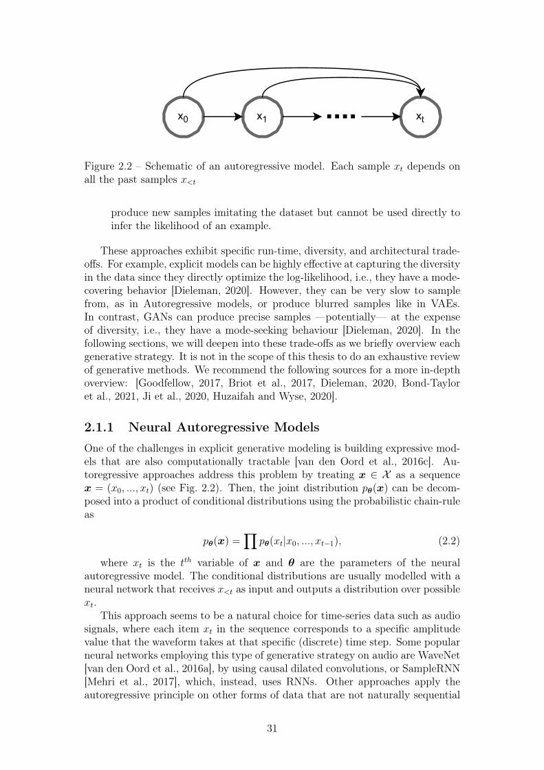
2.2 Schematic of an autoregressive model. Each sample xt depends onall the past samples x<t . . . . . . . . . . . . . . . . . . . . . . . 31

12

2.3 Schematic depiction of Normalizing Flows. The term ‘flow’ refersto the stream followed by samples z0 ∼ N (0, I) as they are moldedby the sequence of transformations f1, ..., fT . The term ‘normal-izing’ refers to the fact that the probability mass is preservedthroughout the transformations. Note that the last iterate in gresults in a more flexible distributions of zT−1 over the values ofthe data x (being zT = x and zt = ft(zt−1)). . . . . . . . . . . . 33

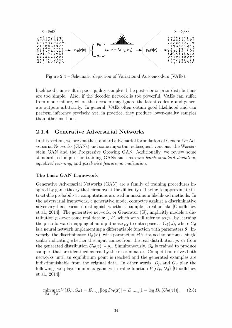
2.4 Schematic depiction of Variational Autoencoders (VAEs). . . . . . 342.5 GAN framework . . . . . . . . . . . . . . . . . . . . . . . . . . . . 352.6 Progressive Growing of GANs as illustrated in [Karras et al., 2017].

Training starts with both G and D having a low spatial resolutionof 4×4 pixels and, as training progresses, new layers containingup-sampling blocks are added to G and D, increasing the spatialresolution of the generated images. . . . . . . . . . . . . . . . . . 37

2.7 Layer fading as illustrated by Karras et al. [2017]. The output ofevery new layer in G and D is interpolated by a factor α with theprevious layer’s output. This transition from low-resolution data,e.g., 16× 16 pixel images (a), to high-resolution data, e.g., 32× 32pixel images (c), is illustrated in the transition (b), where the lay-ers that operate on the new resolution are treated as a residualblock with α increasing linearly from 0 to 1. Here 2× and 0.5×refer to doubling and halving the resolution using nearest neigh-bor up-sampling and average pooling, respectively, for G and D.toRGB is a 1 × 1 convolutional layer that projects feature mapsto the data space (e.g., RGB channels of an image or magnitude,and phase components of a spectrogram) and fromRGB does thereverse. When training the discriminator on a real batch, the datais down-scaled to match the current resolution of the network. . . 37

2.8 Schematic of the VQCPC training framework applied to audio inanalogy to that described by Hadjeres and Crestel [2020] for sym-bolic music. . . . . . . . . . . . . . . . . . . . . . . . . . . . . . . 42

4.1 On the left: the architecture of the generator G; on the right: thearchitecture of D mirroring G’s configuration. . . . . . . . . . . . 62

4.2 Conditional GAN training scheme. . . . . . . . . . . . . . . . . . 634.3 Architecture of the Inception Model for image classification as de-

scribed by Szegedy et al. [2016]. We adapt this architecture toaudio and train our own inception model on instrument, and/orpitch classification. . . . . . . . . . . . . . . . . . . . . . . . . . . 65

6.1 Conditional GAN training scheme. . . . . . . . . . . . . . . . . . 796.2 DrumGAN’s Graphical User Interface (GUI) developed by Cyran

Aouameur. . . . . . . . . . . . . . . . . . . . . . . . . . . . . . . . 836.3 A frame-shot from the teaser . . . . . . . . . . . . . . . . . . . . . 84

7.1 Training diagram for DarkGAN. Note that the temperature valueT is parametrizing a Sigmoid activation function in both the techerPANN and the student D, as explained in Section 2.2 . . . . . . . 91

7.2 Out-of-distribution average attribute correlation ρδ (see Sec. 7.3) . 96

13

7.3 Increment consistency ∆F δk (see Sec.7.3) . . . . . . . . . . . . . . 97

8.1 Updated schematic of VQCPC incorporating the Constant-Q Trans-form (CQT). . . . . . . . . . . . . . . . . . . . . . . . . . . . . . . 103

8.2 Proposed architecture for VQCPC-GAN (see Sec. 8.2.2). . . . . . 1048.3 Proposed architecture for VQCPC-GAN (see Sec. 8.2.2). . . . . . 105

9.1 Schematic depiction of the architecture and training procedure. . 1159.2 Spectrograms of (a) original audio excerpts, (b) corresponding

32kbit/s MP3 versions, and (c), (d), (e) restorations with differentnoise z randomly sampled from N (0, I). . . . . . . . . . . . . . . 119

9.3 Violin plots of objective metrics for stochastic (sto), deterministic(det) models and MP3 baselines (mp3), for different compressionrates (16 kbit/s, 32kbit/s, 64kbit/s). Higher values are better forODG, DI and SNR; lower values are better for LSD and MSE. . . 120

9.4 Frequency profiles of 50 random 4-second-long excerpts from thetest set (in 32kbit/s) for different random input noise vectors z.The blue lines show the profiles of the individual samples, thegreen line shows the mean profile of the excerpts, the dotted redline shows the mean of the high-quality excerpts for comparison.It becomes clear that z is strongly correlated with the energy inthe upper bands and that a specific z yields a consistent overallcharacteristic. . . . . . . . . . . . . . . . . . . . . . . . . . . . . . 125

10.1 Example of BassNet’s behavior when confronted to out-of-domaininput. BassNet(bottom-most track) adjusts its output’s spectralenvelope to the kick’s attacks, and reacts to the percussion’s “tonal-ity”. . . . . . . . . . . . . . . . . . . . . . . . . . . . . . . . . . . 134

10.2 Example of the integration of AI-based prototypes in a popularmusic production workflow . . . . . . . . . . . . . . . . . . . . . . 138

14

List of Tables

3.1 Summary of the most important neural audio synthesis approaches 49

5.1 Audio representation configuration . . . . . . . . . . . . . . . . . 705.2 Unconditional models (i.e., trained without pitch conditioning).

Higher is better for PIS and IIS, lower is better for PKID, IKIDand FAD. . . . . . . . . . . . . . . . . . . . . . . . . . . . . . . . 70

5.3 Conditional models. Higher is better for PIS and IIS, lower isbetter for PKID, IKID and FAD. . . . . . . . . . . . . . . . . . . 71

5.4 Metrics of post-processed real data for lossy transformations. Higheris better for PIS and IIS, lower is better for PKID, IKID and FAD. 71

5.5 Training, sampling and inversion times for each model . . . . . . . 72

6.1 Results of Inception Score (IS, higher is better), Kernel InceptionDistance (KID, lower is better) and Fréchet Audio Distance (FAD,lower is better), scored by DrumGAN under different conditioningsettings, against real data and the unconditional baseline. Themetrics are computed over 50k samples, except for val feats, where30k samples are used (i.e., the validation set size). . . . . . . . . . 81

6.2 Results of Kernel Inception Distance (KID) and Fréchet AudioDistance (FAD), scored by the U-Net baseline [Ramires et al., 2020]when conditioning the model on feature configurations from thereal data and on randomly sampled features. The metrics arecomputed over 11k samples (i.e., the Freesound drum subset size). 81

6.3 Mean accuracy for the feature coherence tests on samples generatedwith the baseline U-Net [Ramires et al., 2020] and DrumGAN. . . 81

7.1 PIS, IIS, KID and FAD (see Sec. 4.3) . . . . . . . . . . . . . . . . 937.2 A few examples of attribute correlation coefficients ρi(α,α) (see

Sec. 7.3). The whole table can be found in Appendix B. . . . . . . 94

8.1 IIS, PIS, KID, and FAD (Sec. 4.3), scored by VQCPC-GAN andbaselines. The metrics are computed over 25k samples. . . . . . . 106

9.1 Architecture details of generator G and discriminator D for 4-second-long excerpts (i.e., 336 spectrogram frames), where (·)-brackets mark information applying only to G, and informationin [·]-brackets applies only to D. During training, no padding isused in the time dimension for G resulting in a shrinking of itsoutput to 212 time steps. . . . . . . . . . . . . . . . . . . . . . . . 117

15

9.2 Results of objective metrics for stochastic (sto), deterministic (det)models and MP3 baselines (mp3), for different compression rates(16kbit/s, 32kbit/s, 64kbit/s). Higher values are better for ODG,DI and SNR; lower values are better for LSD and MSE. . . . . . . 121

9.3 Mean Opinion Score (MOS) of absolute ratings for different com-pression rates. We compare the stochastic (sto) versions againstthe deterministic baselines (det), the MP3-encoded lower anchors(mp3 ) and the original high-quality audio excerpts. . . . . . . . . 123

1 A few examples of attribute correlation coefficients ρi(α, α) (seeSec. 7.3). . . . . . . . . . . . . . . . . . . . . . . . . . . . . . . . . 148

2 Attribute correlation coefficients ρi(α, α) (see Sec. 7.3). . . . . . . 1493 A few examples of attribute correlation coefficients ρi(α, α) (see

Sec. 7.3). . . . . . . . . . . . . . . . . . . . . . . . . . . . . . . . . 150

16

List of publications

〈EUSIPCO2019〉Javier Nistal, Stefan Lattner, and Gaël Richard. Comparing Represen-tations for Audio Synthesis Using Generative Adversarial Networks InProceedings of the 28th European Signal Processing Conference (EUSIPCO2019), pages 161-165, Amsterdam, The Netherlands, November 2019. EU-SIPCO. doi: 10.23919/Eusipco47968.2020.9287799. https://ieeexplore.ieee.org/document/9287799.

〈ISMIR2020〉Javier Nistal, Stefan Lattner, and Gaël Richard. DrumGAN: Synthesisof Drum Sounds with Timbral Feature Conditioning Using Generative Ad-versarial Networks. In Proceedings of the 21st International Society forMusic Information Retrieval Conference (ISMIR), pages 590–597, Mon-treal, Canada, October 2020. ISMIR. URL http://archives.ismir.net/ismir2020/paper/000255.pdf.

〈ISMIR2021〉Javier Nistal, Stefan Lattner, and Gaël Richard. DarkGAN: ExploitingKnowledge Distillation for Comprehensible Audio Synthesis With GANs.In Proceedings of the 22nd International Society for Music InformationRetrieval Conference (ISMIR), Virtual, November 2021. ISMIR. https://hal.archives-ouvertes.fr/hal-03349492/document.

〈WASPAA2021〉Javier Nistal, Cyran Aouameur, Stefan Lattner, and Gaël Richard. VQCPC-GAN: Variable- Length Adversarial Audio Synthesis using Vector-QuantizedContrastive Predictive Coding. In IEEE Workshop on Applications of Sig-nal Processing to Audio and Acoustics (WASPAA), Oct 2021, New Paltz,United States. https://hal.telecom-paris.fr/hal-03413460/document.

〈MDPI2021〉Stefan Lattner, and Javier Nistal. Stochastic Restoration of Heavily Com-pressed Musical Audio using Generative Adversarial Networks. Electronics10, no. 11: 1349. MDPI. https://doi.org/10.3390/electronics10111349.

〈TISMIR2022〉Emanuel Deruty, Martin Grachteen, Stefan Lattner, Javier Nistal, andCyran Aouameur. On the development and practice of AI technologyfor contemporary popular music production. Transactions of the Interna-tional Society for Music Information Retrieval (TISMIR)

17

Notation

We generally use bold symbols to indicate vectors (lowercase) and matrices (up-percase). Uppercase symbols may be also used to indicate constants. Whentheory is applicable to either scalars, vectors or n-dimensional algebraic objects(tensors), we employ lowercase symbols. We indicate probability distribution byp(·). We often add a subscript to probability densities, e.g. pθ(x), to indicate thedistribution of random variables x with distributional parameters θ. The symbolE(·) represents the expected value operator. Finally, we represent the samplingor simulation of variates x from a distribution p(x) using the notation x ∼ p(x).

18

Abbreviations

AE AutoencoderAI Artificial IntelligenceCNN Convolutional Neural NetworkCPC Contrastive Predictive CodingCPM Contemporary Popular MusicCQT Constant-Q TransformCV Computer VisionDAW Digital Audio WorkstationDL Deep LearningDNN Deep Neural NetworkDSP Digital Signal ProcessingFAD Fréchet Audio DistanceFFT Fast Fourier TransformFM Frequency ModulationGAN Generative Adversarial NetworkGNN Generative Neural NetworkGP Gradient PenaltyGUI Graphical User InterfaceIAF Inverse Autoregressive FlowIS Inception ScoreIIS Instrument Inception ScoreKD Knowledge DistillationLFO Low-Frequency OscillatorLSTM Long Short-Term MemoryMIDI Musical Instrument Digital InterfaceMFCC Mel Frequency Cepstrum CoefficientsML Machine LearningNAM Neural Autoregressive ModelNAS Neural Audio SynthesizerNF Normalizing FlowPGAN Progressive Growing GANPIS Pitch Inception ScoreRNN Recurrent Neural NetworkSTFT Short-Time Fourier TransformVAE Variational AutoencoderVST Virtual Studio TechnologyVQ Vector QuantizationWGAN Wasserstein GAN

19

20

Chapter 1

Introduction

“I dream of instruments obedient to my thought and which with theircontribution of a whole new world of unsuspected sounds, will lendthemselves to the exigencies of my inner rhythm”

— Edgard Varèse, 1917

Audio synthesizers are electronic musical instruments that generate artificialsounds under some parametric control. Popularized during the 70s, these devices,now ubiquitous in most of the music we listen to, have since reshaped musicproduction, giving birth to new music genres and novel paradigms for musicalinteraction and expression.

While synthesizers have evolved since they first appeared, two fundamentalchallenges are still faced. One is the development of genuinely accessible anduser-driven synthesis systems, responding to semantically intuitive parameters.Fig. 1.1 shows the interface of Sonicbits’ Exakt Lite, an “intuitive and user-friendlyFM synthesizer plugin.”1 Waveform, filter, frequency modulation, etc.: the vastand complex parameter space that synthesizers afford is an unquestioned sourceof inspiration for a few, yet, for the many, they pose an obstacle that slows downthe creative process. This process may seem analogous to any other musicalinstrument: one must train hard to fully unveil its sonic possibilities, e.g., per-forming vibrato or finger-tapping in a guitar to achieve different timbres requiresexpertise. However, anyone can understand the guitar’s interaction protocol, i.e.,the set of mechanic rules to obtain a specific sound. Synthesizers, on the contrary,require strong signal processing knowledge to guide the system towards a specificsound purposely. The main barrier resides in the semantic gap between the syn-thesis parameters and the musician’s cognitive factors driving creative thoughts.The synthesizer’s language is signal processing, whereas the artist’s language con-cerns abstract properties such as emotions, perception, experiences, or musicalaesthetics, to name a few. Under current systems, it is the user’s responsibilityto translate this unstructured context into the synthesizer’s parameter space andnot the opposite; this is the synth incorporating parameters that can respondto the musician’s language. An overview of this process is further illustrated inFig. 1.2.

The second challenge is designing “universal,” source-agnostic synthesis tech-niques that can approximate any timbre and offer generic workflows. As we

1https://www.sonicbits.com/exakt-lite.html

21

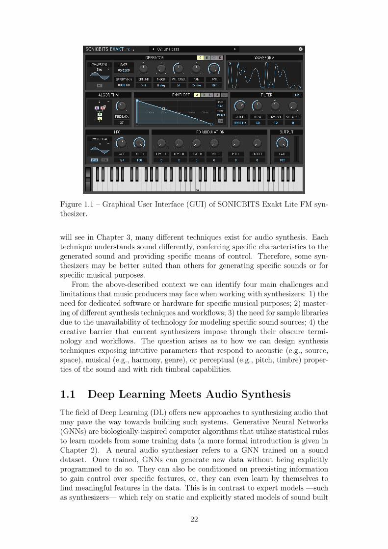
Figure 1.1 – Graphical User Interface (GUI) of SONICBITS Exakt Lite FM syn-thesizer.

will see in Chapter 3, many different techniques exist for audio synthesis. Eachtechnique understands sound differently, conferring specific characteristics to thegenerated sound and providing specific means of control. Therefore, some syn-thesizers may be better suited than others for generating specific sounds or forspecific musical purposes.

From the above-described context we can identify four main challenges andlimitations that music producers may face when working with synthesizers: 1) theneed for dedicated software or hardware for specific musical purposes; 2) master-ing of different synthesis techniques and workflows; 3) the need for sample librariesdue to the unavailability of technology for modeling specific sound sources; 4) thecreative barrier that current synthesizers impose through their obscure termi-nology and workflows. The question arises as to how we can design synthesistechniques exposing intuitive parameters that respond to acoustic (e.g., source,space), musical (e.g., harmony, genre), or perceptual (e.g., pitch, timbre) proper-ties of the sound and with rich timbral capabilities.

1.1 Deep Learning Meets Audio SynthesisThe field of Deep Learning (DL) offers new approaches to synthesizing audio thatmay pave the way towards building such systems. Generative Neural Networks(GNNs) are biologically-inspired computer algorithms that utilize statistical rulesto learn models from some training data (a more formal introduction is given inChapter 2). A neural audio synthesizer refers to a GNN trained on a sounddataset. Once trained, GNNs can generate new data without being explicitlyprogrammed to do so. They can also be conditioned on preexisting informationto gain control over specific features, or, they can even learn by themselves tofind meaningful features in the data. This is in contrast to expert models —suchas synthesizers— which rely on static and explicitly stated models of sound built

22

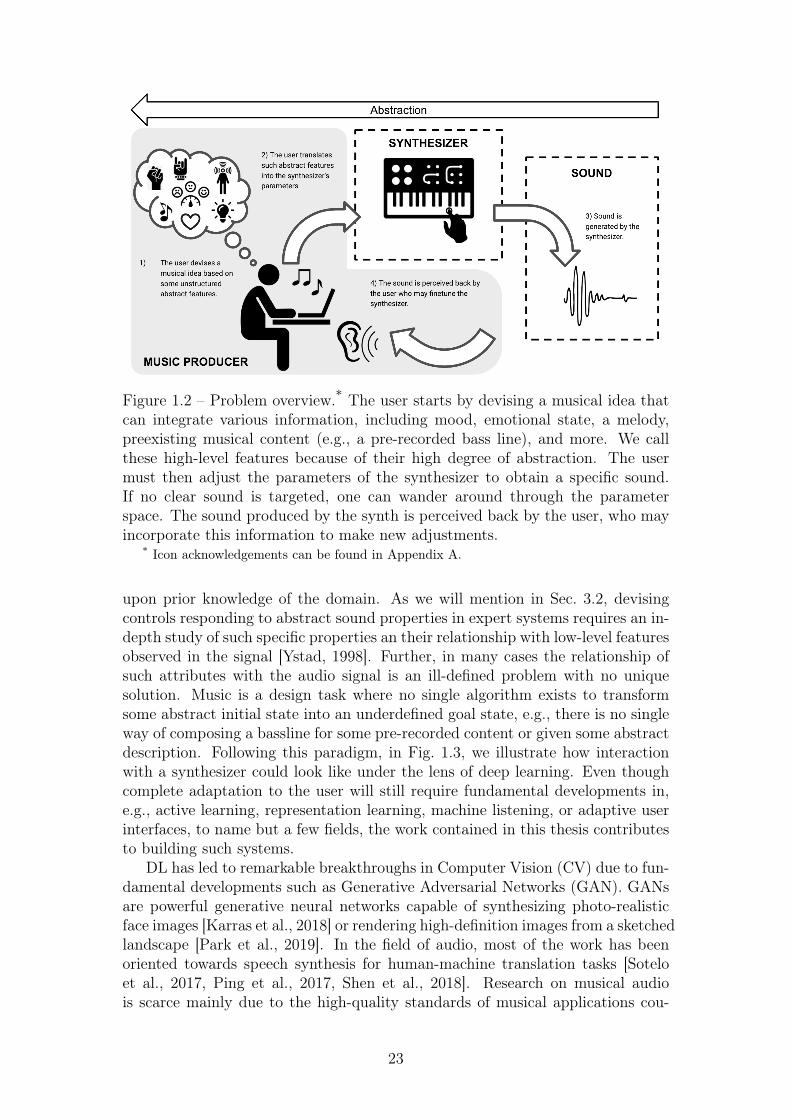
Figure 1.2 – Problem overview.* The user starts by devising a musical idea thatcan integrate various information, including mood, emotional state, a melody,preexisting musical content (e.g., a pre-recorded bass line), and more. We callthese high-level features because of their high degree of abstraction. The usermust then adjust the parameters of the synthesizer to obtain a specific sound.If no clear sound is targeted, one can wander around through the parameterspace. The sound produced by the synth is perceived back by the user, who mayincorporate this information to make new adjustments.

* Icon acknowledgements can be found in Appendix A.

upon prior knowledge of the domain. As we will mention in Sec. 3.2, devisingcontrols responding to abstract sound properties in expert systems requires an in-depth study of such specific properties an their relationship with low-level featuresobserved in the signal [Ystad, 1998]. Further, in many cases the relationship ofsuch attributes with the audio signal is an ill-defined problem with no uniquesolution. Music is a design task where no single algorithm exists to transformsome abstract initial state into an underdefined goal state, e.g., there is no singleway of composing a bassline for some pre-recorded content or given some abstractdescription. Following this paradigm, in Fig. 1.3, we illustrate how interactionwith a synthesizer could look like under the lens of deep learning. Even thoughcomplete adaptation to the user will still require fundamental developments in,e.g., active learning, representation learning, machine listening, or adaptive userinterfaces, to name but a few fields, the work contained in this thesis contributesto building such systems.

DL has led to remarkable breakthroughs in Computer Vision (CV) due to fun-damental developments such as Generative Adversarial Networks (GAN). GANsare powerful generative neural networks capable of synthesizing photo-realisticface images [Karras et al., 2018] or rendering high-definition images from a sketchedlandscape [Park et al., 2019]. In the field of audio, most of the work has beenoriented towards speech synthesis for human-machine translation tasks [Soteloet al., 2017, Ping et al., 2017, Shen et al., 2018]. Research on musical audiois scarce mainly due to the high-quality standards of musical applications cou-

23

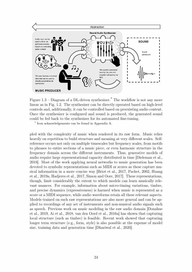
Figure 1.3 – Diagram of a DL-driven synthesizer.* The workflow is not any morelinear as in Fig. 1.2. The synthesizer can be directly operated based on high-levelcontrols and, additionally, it can be controlled based on preexisting audio content.Once the synthesizer is configured and sound is produced, the generated soundcould be fed back to the synthesizer for its automated fine-tuning.

* Icon acknowledgements can be found in Appendix A.

pled with the complexity of music when rendered in its raw form. Music reliesheavily on repetition to build structure and meaning at very different scales. Self-reference occurs not only on multiple timescales but frequency scales, from motifsto phrases to entire sections of a music piece, or even harmonic structure in thefrequency domain across the different instruments. Thus, generative models ofaudio require large representational capacity distributed in time [Dieleman et al.,2018]. Most of the work applying neural networks to music generation has beendevoted to symbolic representations such as MIDI or scores as these capture mu-sical information in a more concise way [Briot et al., 2017, Pachet, 2002, Huanget al., 2019a, Hadjeres et al., 2017, Simon and Oore, 2017]. These representations,though, limit considerably the extent to which models can learn musically rele-vant nuances. For example, information about micro-timing variations, timbre,and precise dynamics (expressiveness) is harmed when music is represented as ascore or a MIDI sequence, while audio waveforms retain all these relevant aspects.Models trained on such raw representations are also more general and can be ap-plied to recordings of any set of instruments and non-musical audio signals suchas speech. Previous work on music modeling in the raw audio domain [Donahueet al., 2019, Ai et al., 2018, van den Oord et al., 2016a] has shown that capturinglocal structure (such as timbre) is feasible. Recent work showed that capturinglonger term structure (e.g., form, style) is also possible at the expense of modelsize, training data and generation time [Dhariwal et al., 2020].

24

1.2 Scope and ContributionsThis thesis researches a broad set of applications of GANs to musical soundsynthesis tasks. The main goal is to study and develop novel tools for musicproduction that can offer the user intuitive and, simultaneously, inspiring meansof sound manipulation, e.g., by controlling parameters that respond to percep-tual properties of the sound or other high-level features. Further motivated inChapter 2, an adversarial scheme is preferred over other generative modelingstrategies (e.g., autoregressive, variational) as GANs evidence a good compromisebetween generation time, sample quality, and diversity. These considerations areof great importance in building commercially viable solutions that can run on aconventional computer while meeting the audio quality standards and real-timeperformance required in music production.

In order to steer the synthesis process, we are interested in conditioning theGAN on information describing musical or perceptual properties of the sound,namely features describing timbre (e.g., brightness, boominess), instrument cat-egories (e.g., violin, piano), or sound event categories (e.g., sonar, mantra).Such annotations are obtained from 1) pre-existing hand-labeled information,2) human-engineered feature extractors, or 3) representations learned using pre-trained automatic audio tagging systems. A sound synthesizer built upon such amodel would have many applications and speed the music production workflowtremendously while making it more intuitive and user-driven.

The contributions of this thesis can be summarized in the following points:

1. We provide insights on the performance of several audio signal represen-tations (e.g., raw waveform, spectrogram) for musical audio synthesis withGANs.

2. We study a variety of conditional generation tasks with GANs, exploringdifferent sources of conditional information in order to provide to the usercreative means of sound manipulation.

3. We demonstrate the capability of a single GAN architecture to model awide variety of sound sources, from percussive and pitched instruments tochainsaw sounds and music.

4. A framework for generating audio with variable duration is proposed byconditioning the GAN on sequential features learned through self-supervisedmethods.

5. As a result of our research, we build two VST plugins for synthesizing highresolution (i.e., 44.1 kHz sample-rate) sounds such as drums in DrumGAN,or chainsaw sounds, in ChainsawGAN.

6. We perform a user study with professional musicians who created musicwith various in-house ML-driven tools for music production. We reporttheir feedback and conclude thereby.

25

1.3 Ethical ConsiderationsAutomation is increasingly becoming part of standard technological solutions andservices (e.g., smartphones, cars, social networks), providing these with intelli-gence to plan and initiate actions autonomously. It is vital to raise awarenessabout the implications that such solutions have in creative activities like music.Deep learning-based generative models fall into one of two control principles: onewhere the user directly controls all aspects of the synthesis, akin to playing aninstrument, and another whereby the system takes complete control. The de-ployment of fully automated audio generation systems can severely obscure andconceal the artist’s role in the music creation process. While such systems areinteresting from a scientific perspective to establish limits on technology, we be-lieve that they do not add any value from a music innovation point of view. Theauthor of this thesis is sensitive to the music community. This work does nothereby seek or claim to replace musicians in any way. On the contrary, we oughtto develop tools that can democratize music production and help artists focus oncreative aspects of music rather than technical ones.

Another critical aspect to be considered is the carbon footprint of traininglarge-scale deep learning systems. We estimate to have emitted an average of 18kg CO2 per model, assuming a standard carbon efficiency of the grid. This isequivalent to 63 Km driven by an average car or to 7.8 Kgs of coal burned. Oneof our aims for future work is to train efficient, compact models that require lessamount of training time and that can run on a personal computer.

1.4 Document OrganisationThe first three chapters of this thesis are dedicated to presenting the backgroundand related work. Chapters 5 to 10 comprise a collection of six articles listedat the beginning of this document. The first four of these (chapters 5 to 8)constitute the main contribution of the thesis and cover several audio synthesistasks with GANs. Chapters 9 and 10 are collaboration journal articles focusingrespectively on: (i) audio enhancement of MP3-music using GANs and (ii) acritical perspective on AI-centered musical research in the context of musicalinnovation in contemporary popular music. More in detail, the rest of this thesisis organized as follows:

Chapter 2: Background. In this chapter we provide some basics ondifferent deep learning strategies and various audio signal representationsthat are required for the proper understanding of this thesis.

Chapter 3: Related work. This chapter overviews all the relevant litera-ture on neural audio synthesis as well as techniques prior the deep learningera.

Chapter 4: Methodology. This chapter describes the common method-ologies followed throughout the experiments, describing in detail the GANarchitecture, the datasets and the evaluation metrics.

26

Chapter 5: Comparing Representations for Audio Synthesis Us-ing GANs. This chapter presents the results of our first work comparingrepresentations for adversarial audio synthesis of tonal instrument sounds.

Chapter 6: DrumGAN: Synthesis of Drum Sounds with TimbralFeature Conditioning Using GANs. In this chapter we present Drum-GAN, a GAN synthesizer of drum sounds that can be controlled based onperceptual features describing timbre. We also introduce a VST plugin im-plementation of DrumGAN capable of generating audio that meets musicproduction standards in terms of quality.

Chapter 7: DarkGAN: Exploiting Knowledge Distillation for Com-prehensible Audio Synthesis with GANs. In this chapter we presentDarkGAN, a framework for learning high-level feature controls in a GANsynthesizer by distilling knowledge from a pre-trained audio-tagging system.

Chapter 8: VQCPC-GAN: Variable-length Adversarial Audio Syn-thesis using Vector-Quantized Contrastive Predictive Coding. Thischapter presents VQCPC-GAN, an adversarial framework for synthesiz-ing variable-length audio by exploiting a self-supervised learning techniquecalled Vector-Quantized Contrastive Predictive Coding (VQCPC).

Chapter 9: Stochastic Restoration of Heavily Compressed MusicalAudio using GANs. In this chapter we describe a GAN that restoresheavily compressed MP3 music to its high-quality, uncompressed form.

Chapter 10: On the Development and Practice of AI Technologyfor Contemporary Popular Music Production. This chapter formu-lates Sony CSL music team’s vision on how to conduct music technologyresearch in practice, involving the artist in the process and by releasingcommercially viable music as a means for implicit validation. To this end,we report on our collaborations with professional musicians, in which weharmonize the use of AI-based tools with their music production workflow.

Chapter 11: General Conclusion. Finally, in this chapter some generalconclusions are drawn, and, ultimately, we suggest directions for futureresearch.

27

28

Chapter 2

Background

This thesis explores the generation of musical sounds using Generative Adver-sarial Networks (GANs) [Goodfellow et al., 2014] by exploiting different sourcesof conditional information. Our goal is to provide insights into musically con-trollable adversarial audio synthesis and, ultimately, implement tools that canhelp professional artists in music production settings to enhance creativity whileoptimizing their workflows.

This chapter provides some ground knowledge on the various topics uponwhich this thesis builds. First, Section 2.1 briefly describes the main approachesto generative modeling (autoregressive, variational autoencoders, adversarial, andflow-based), paying special attention to GANs and some standard techniques suchas progressive growing [Karras et al., 2017] or the Wasserstein objective [Arjovskyet al., 2017] (see Sec. 2.1.4). Section 2.2 introduces Knowledge Distillation (KD)[Hinton et al., 2015] and Dark Knowledge [Hinton et al., 2014] (KD is employedin Chapter 7 to perform data-free learning of semantically meaningful parametersin DarkGAN [Nistal et al., 2021b]). Next, Section 2.3 provides some backgroundon self-supervised learning of sequences and introduces Vector-Quantized Con-trastive Predictive Coding (VQCPC), which is used in Chapter 8 to address theproblem of variable-length audio generation in GANs. Finally, in Section 2.4, wegive an overview of some common representations of audio that will be comparedin the context of audio synthesis with GANs (see Chapter 5).

2.1 Generative Neural NetworksGenerative Neural Networks are a family of generative modeling strategies thatemploy neural networks to model the distribution pX (x) of some random processproducing observations from a dataset X with samples x ∈ X . Specifically, wefocus our attention on likelihood-based models that learn via the principle ofMaximum Likelihood Estimation (MLE): learning the model’s parameters θ sothat the likelihood of observing the data x ∈ X is maximized. This process isformulated as

θ := arg maxθ

∑x∈X

log pθ(x), (2.1)

where pθ(x) is the likelihood or, in other words, the probability of x ∈ Xunder the model with parameters θ. Note that this is done in the log space for

29

Likelihood-based Generative Models

Explicit

-GANs

Implicit

- Autoregressive - Normalizing Flows

Exact

-VAEs

Approximate

Figure 2.1 – Taxonomy of Generative Neural Networks [Goodfellow, 2017]. Meth-ods differ in how they represent or approximate the likelihood. Explicit densityestimation methods provide means to directly maximize the likelihood pθ(x).Among these, the density may be computationally tractable, as in Autoregres-sive or Flow-based models, or it may be intractable, as in VAEs, meaning thatit is necessary to make some approximations to maximize the likelihood. In con-trast, implicit models do not explicitly represent a probability distribution overthe data space. Instead, the model provides some way of interacting less directlywith this probability distribution, typically by learning to draw samples from it.For example GANs can generate a sample x ∼ pθ(x) but cannot directly computepθ(x).

computational simplicity (i.e., products become additions) and numerical stabil-ity. This can also be thought as minimizing the KL-Divergence between the datadistribution pX(x) and the model distribution pθ(x) [Goodfellow, 2017]. Oncetrained, generative models can be used to draw new samples x ∼ pθ(x) as ifthey came from the training distribution pX (x) (i.e., pθ(x) ≈ pX (x)). In order togain control over the samples we draw from the generative model, we can feed aconditioning signal c, containing side information about the kind of samples wewant to generate. The model is then trained to fit the conditional likelihood dis-tribution pθ(x|c) instead of pθ(x). For simplicity, we refer to the unconditionaldistribution in the theoretical descriptions that follow this section.

Generative modeling strategies differ in the way they represent or approximatethe likelihood (see Fig. 2.1). Two main approaches exist:

• Explicit density estimation models provide means of computing pθ(x)and can explicitly maximize the likelihood as formulated in (2.1). Amongthese, two different strategies exist to define a tractable expression. Bycarefully designing the neural network architecture, exact methods can de-fine pθ(x) so that it is computationally tractable. Popular examples ofthese are Neural Autoregressive Models (see 2.1.1) or Normalizing Flows(see 2.1.2). Other methods approximate the likelihood by e.g., maximizinga lower-bound as in Variational Autoencoders (see 2.1.3).

• Implicit density estimationmodels do not explicitly define the likelihoodand, instead, offer indirect ways of interacting with pθ(x). For example,Generative Adversarial Networks [Goodfellow et al., 2014] can be used to

30

x0 x1 xt

Figure 2.2 – Schematic of an autoregressive model. Each sample xt depends onall the past samples x<t

produce new samples imitating the dataset but cannot be used directly toinfer the likelihood of an example.

These approaches exhibit specific run-time, diversity, and architectural trade-offs. For example, explicit models can be highly effective at capturing the diversityin the data since they directly optimize the log-likelihood, i.e., they have a mode-covering behavior [Dieleman, 2020]. However, they can be very slow to samplefrom, as in Autoregressive models, or produce blurred samples like in VAEs.In contrast, GANs can produce precise samples —potentially— at the expenseof diversity, i.e., they have a mode-seeking behaviour [Dieleman, 2020]. In thefollowing sections, we will deepen into these trade-offs as we briefly overview eachgenerative strategy. It is not in the scope of this thesis to do an exhaustive reviewof generative methods. We recommend the following sources for a more in-depthoverview: [Goodfellow, 2017, Briot et al., 2017, Dieleman, 2020, Bond-Tayloret al., 2021, Ji et al., 2020, Huzaifah and Wyse, 2020].

2.1.1 Neural Autoregressive Models

One of the challenges in explicit generative modeling is building expressive mod-els that are also computationally tractable [van den Oord et al., 2016c]. Au-toregressive approaches address this problem by treating x ∈ X as a sequencex = (x0, ..., xt) (see Fig. 2.2). Then, the joint distribution pθ(x) can be decom-posed into a product of conditional distributions using the probabilistic chain-ruleas

pθ(x) =∏

pθ(xt|x0, ..., xt−1), (2.2)

where xt is the tth variable of x and θ are the parameters of the neuralautoregressive model. The conditional distributions are usually modelled with aneural network that receives x<t as input and outputs a distribution over possiblext.

This approach seems to be a natural choice for time-series data such as audiosignals, where each item xt in the sequence corresponds to a specific amplitudevalue that the waveform takes at that specific (discrete) time step. Some popularneural networks employing this type of generative strategy on audio are WaveNet[van den Oord et al., 2016a], by using causal dilated convolutions, or SampleRNN[Mehri et al., 2017], which, instead, uses RNNs. Other approaches apply theautoregressive principle on other forms of data that are not naturally sequential

31

such as images [van den Oord et al., 2016c,b]. In Chapter 3 we review these andother approaches in detail.

Autoregressive models are very precise methods and can accurately capturecorrelations between the elements xt in the sequential data. They also allow forfast inference (i.e. computing pθ(xt|x<t)). However, due to the sequential scheme,autoregressive models can only generate one sample at a time, becoming veryslow to sample from (e.g., WaveNet [van den Oord et al., 2016a] can take minutesto generate just one second of audio). Also, autoregressive models can sufferfrom the exposure bias problem, i.e., the discrepancy between the conditionalsamples x<t used at training time, which come from the dataset, and those usedfor inference, which are generated by the model [Bengio et al.]. As a result, atgeneration time the error increases over time as the generated samples are fedback into the model.

2.1.2 Normalizing Flows

Other approaches for explicit density estimation that also provide an exact defini-tion of the likelihood are Normalizing Flows (NF) [Rezende and Mohamed, 2015].NFs are a family of procedures for learning flexible posterior distributions throughan iterative procedure. The general idea is to start from an initial random variablez0 following a simple base distribution with known and computationally cheapprobability density function, typically a standard Gaussian distribution. Then, acascade of invertible and differentiable transformations g : fT ◦ fT−1 ◦ ... ◦ f1 ◦ f0is applied using the change of variables formula to produce a sample from thedataset as x = g(z0) (see Fig. 2.3). The log-likelihood can then be expressed as

log pθ(x) = log pz0(z)−T∑t=1

log∣∣∣ det

∂ft∂ft−1

∣∣∣ = log pz0(z)− log∣∣∣ det Jg(z0)

∣∣∣, (2.3)

where the Jacobian Jg(z0) is a matrix of all partial derivatives of g w.r.t. z0.The density pθ is tractable if the density pz and the determinant of the Jacobianof g are tractable. We can think of this process as follows: the density of the basedistribution z0 gets molded by each transformation in g in order to produce anincreasingly richer output distribution from which to sample x.

Many types of NFs exist satisfying the invertibility and tractability require-ments for g and Jg respectevely, e.g., Planar Flows (PFs), Masked AutoregressiveFlows (MAFs), Inverse Autoregressive Flows (IAFs). Each formulation exhibitsdifferent inference-sampling time trade-offs, e.g., IAFs can generate samples fastalthough computing the likelihood of new data points is slow [Bond-Taylor et al.,2021]. Also, the invertibility requirement for g enforces the variables z0 to havethe same dimensionality as x, constraining the model’s architecture and parame-ter efficiency. As a result, flow-based models require rather deep architectures tobe effective.

2.1.3 Variational Autoencoders

To overcome some of the disadvantages imposed by the design requirements ofmodels with tractable density functions (e.g., slow sampling time in NAMs, pa-

32

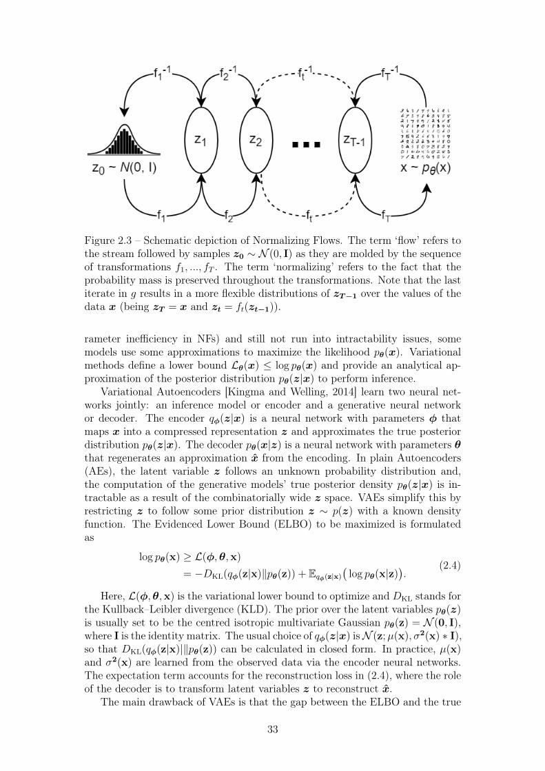
Figure 2.3 – Schematic depiction of Normalizing Flows. The term ‘flow’ refers tothe stream followed by samples z0 ∼ N (0, I) as they are molded by the sequenceof transformations f1, ..., fT . The term ‘normalizing’ refers to the fact that theprobability mass is preserved throughout the transformations. Note that the lastiterate in g results in a more flexible distributions of zT−1 over the values of thedata x (being zT = x and zt = ft(zt−1)).

rameter inefficiency in NFs) and still not run into intractability issues, somemodels use some approximations to maximize the likelihood pθ(x). Variationalmethods define a lower bound Lθ(x) ≤ log pθ(x) and provide an analytical ap-proximation of the posterior distribution pθ(z|x) to perform inference.

Variational Autoencoders [Kingma and Welling, 2014] learn two neural net-works jointly: an inference model or encoder and a generative neural networkor decoder. The encoder qφ(z|x) is a neural network with parameters φ thatmaps x into a compressed representation z and approximates the true posteriordistribution pθ(z|x). The decoder pθ(x|z) is a neural network with parameters θthat regenerates an approximation x from the encoding. In plain Autoencoders(AEs), the latent variable z follows an unknown probability distribution and,the computation of the generative models’ true posterior density pθ(z|x) is in-tractable as a result of the combinatorially wide z space. VAEs simplify this byrestricting z to follow some prior distribution z ∼ p(z) with a known densityfunction. The Evidenced Lower Bound (ELBO) to be maximized is formulatedas

log pθ(x) ≥ L(φ,θ,x)

= −DKL(qφ(z|x)‖pθ(z)) + Eqφ(z|x)(

log pθ(x|z)).

(2.4)

Here, L(φ,θ,x) is the variational lower bound to optimize and DKL stands forthe Kullback–Leibler divergence (KLD). The prior over the latent variables pθ(z)is usually set to be the centred isotropic multivariate Gaussian pθ(z) = N (0, I),where I is the identity matrix. The usual choice of qφ(z|x) isN (z;µ(x), σ2(x) ∗ I),so that DKL(qφ(z|x)|‖pθ(z)) can be calculated in closed form. In practice, µ(x)and σ2(x) are learned from the observed data via the encoder neural networks.The expectation term accounts for the reconstruction loss in (2.4), where the roleof the decoder is to transform latent variables z to reconstruct x.

The main drawback of VAEs is that the gap between the ELBO and the true

33

qΦ(z|x) pθ(x|z)z ~ N(μx, σx)

x ~ pX(x) x ~ pθ(x)

μx

σx

Figure 2.4 – Schematic depiction of Variational Autoencoders (VAEs).

likelihood can result in poor quality samples if the posterior or prior distributionsare too simple. Also, if the decoder network is too powerful, VAEs can sufferfrom mode failure, where the decoder may ignore the latent codes z and gener-ate outputs arbitrarily. In general, VAEs often obtain good likelihood and canperform inference precisely, yet, in practice, they produce lower-quality samplesthan other methods.

2.1.4 Generative Adversarial Networks

In this section, we present the standard adversarial formulation of Generative Ad-versarial Networks (GANs) and some important subsequent versions: the Wasser-stein GAN and the Progressive Growing GAN. Additionally, we review somestandard techniques for training GANs such as mini-batch standard deviation,equalized learning, and pixel-wise feature normalization.

The basic GAN framework

Generative Adversarial Networks (GAN) are a family of training procedures in-spired by game theory that circumvent the difficulty of having to approximate in-tractable probabilistic computations aroused in maximum likelihood methods. Inthe adversarial framework, a generative model competes against a discriminativeadversary that learns to distinguish whether a sample is real or fake [Goodfellowet al., 2014]. The generative network, or Generator (G), implicitly models a dis-tribution pX over some real data x ∈ X , which we will refer to as pr, by learningthe push-forward mapping of an input noise pz to data space as Gθ(z), where Gθis a neural network implementing a differentiable function with parameters θ. In-versely, the discriminator Dβ(x), with parameters β is trained to output a singlescalar indicating whether the input comes from the real distribution pr or fromthe generated distribution Gθ(z) ∼ pg. Simultaneously, Gθ is trained to producesamples that are identified as real by the discriminator. Competition drives bothnetworks until an equilibrium point is reached and the generated examples areindistinguishable from the original data. In other words, Dβ and Gθ play thefollowing two-player minimax game with value function V (Gθ, Dβ) [Goodfellowet al., 2014]:

minGθ

maxDβ

V (Dβ, Gθ) = Ex∼pr [logDβ(x)] + Ex∼pg [1− logDβ(Gθ(z))], (2.5)

34

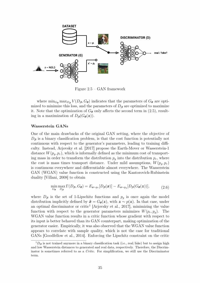
Figure 2.5 – GAN framework

where minGθmaxDβ

V (Dβ, Gθ) indicates that the parameters of Gθ are opti-mized to minimize this loss, and the parameters of Dβ are optimized to maximizeit. Note that the optimization of Gθ only affects the second term in (2.5), result-ing in a maximization of Dβ(Gθ(z)).

Wasserstein GANs

One of the main drawbacks of the original GAN setting, where the objective ofDβ is a binary classification problem, is that the cost function is potentially notcontinuous with respect to the generator’s parameters, leading to training diffi-culty. Instead, Arjovsky et al. [2017] propose the Earth-Mover or Wasserstein-1distanceW (pg, pr), which is informally defined as the minimum cost of transport-ing mass in order to transform the distribution pg into the distribution pr, wherethe cost is mass times transport distance. Under mild assumptions, W (pg, pr)is continuous everywhere and differentiable almost everywhere. The WassersteinGAN (WGAN) value function is constructed using the Kantorovich-Rubinsteinduality [Villani, 2008] to obtain

minGθ

maxDβ

Γ(Dβ, Gθ) = Ex∼pr [Dβ(x)]− Ex∼pg [Dβ(Gθ(z))], (2.6)

where Dβ is the set of 1-Lipschitz functions and pg is once again the modeldistribution implicitly defined by x = Gθ(z), with z ∼ p(z). In that case, underan optimal discriminator or critic1 [Arjovsky et al., 2017], minimizing the valuefunction with respect to the generator parameters minimizes W (pr, pg). TheWGAN value function results in a critic function whose gradient with respect toits input is better behaved than its GAN counterpart, making optimization of thegenerator easier. Empirically, it was also observed that the WGAN value functionappears to correlate with sample quality, which is not the case for traditionalGANs [Goodfellow et al., 2014]. Enforcing the Lipschitz constraint on the critic

1Dβ is not trained anymore in a binary classification task (i.e., real/fake) but to assign highand low Wasserstein distances to generated and real data, respectively. Therefore, the Discrim-inator is sometimes referred to as a Critic. For simplification, we still use the Discriminatorterm.

35

was originally accomplished by clipping the weights of the critic to lie within acompact space [−c, c] [Arjovsky et al., 2017]. The set of functions satisfying thisconstraint is a subset of the k-Lipschitz functions for some k, which depends on cand the critic architecture. An alternative way to enforce the Lipschitz constraintis to constrain the gradient norm of the critic’s output with respect to its input bymeans of Gradient Penalty (GP). GP introduces a penalty on D’s gradient normfor random samples x ∼ pg to circumvent tractability issues [Gulrajani et al.,2017]. Then, the GP-WGAN’s objective is defined as

L = Ex∼pg [Dβ(Gθ(z))]− Ex∼pr [Dβ(x)] + λEx∼pg [(‖∇xDβ(Gθ(z)‖2 − 1)2],(2.7)

where λ is the penalty coefficient and it is typically set to 10, which was found towork well across a variety of architectures and datasets [Gulrajani et al., 2017].Following the original GP-WGAN implementation, normalization methods thatintroduce correlations between the examples in the batch (e.g. batch normaliza-tion) are avoided in favour of layer-wise feature normalization as explained laterin this section.

Progressive Growing of GANs

Progressive growing [Karras et al., 2017] is a training methodology for GANswhere low-resolution data (e.g., down-sampled images or spectrograms) is usedat the beginning of training and then progressively scaled up by adding convo-lutional and up-sampling layers to the networks (see Fig. 2.6). This incrementalprocedure allows the network to first discover large-scale structure in the data andthen progressively shift attention towards finer-grain detail instead of having tolearn the full resolution data directly. Generator and discriminator networks arecommonly mirrored versions of each other and always grow synchronously. Allexisting layers in both networks remain trainable throughout the training pro-cess. When new layers are added to the networks, they are faded in smoothly, asillustrated in Figure 2.7. This reduces any possible perturbations to the alreadywell-trained, smaller-resolution layers. Progressive training has many benefits, in-cluding improved training stability, generation diversity, and a reduced trainingtime.

Mini-Batch Standard Deviation

GANs are prone to cover only a part of the training data variance. Mini-batchdiscrimination [Salimans et al., 2016] is a way of alleviating such a mode failureby providing D with additional information, namely statistics of the respectiveminibatch to simplify the discrimination of real and fake batches. To that end,on the last layers of D, we compute feature statistics across the batch dimension.First, the standard deviation for each feature map in each spatial location (i.e.,the height and width dimensions of the convolutional tensor) is estimated overthe minibatch and averaged over all the features and spatial locations to arriveat a single value. Then, this value is replicated and concatenated to all spatiallocations and over the minibatch, yielding one additional (constant) feature map.

36

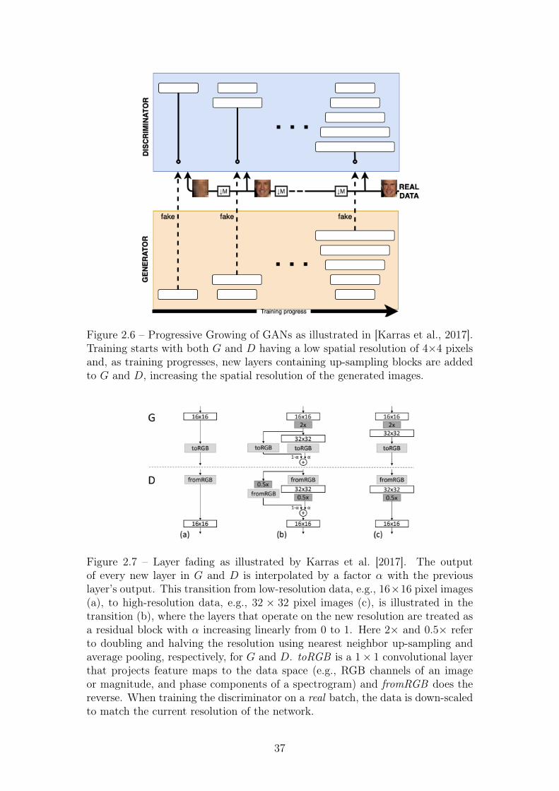
Figure 2.6 – Progressive Growing of GANs as illustrated in [Karras et al., 2017].Training starts with both G and D having a low spatial resolution of 4×4 pixelsand, as training progresses, new layers containing up-sampling blocks are addedto G and D, increasing the spatial resolution of the generated images.

Figure 2.7 – Layer fading as illustrated by Karras et al. [2017]. The outputof every new layer in G and D is interpolated by a factor α with the previouslayer’s output. This transition from low-resolution data, e.g., 16×16 pixel images(a), to high-resolution data, e.g., 32 × 32 pixel images (c), is illustrated in thetransition (b), where the layers that operate on the new resolution are treated asa residual block with α increasing linearly from 0 to 1. Here 2× and 0.5× referto doubling and halving the resolution using nearest neighbor up-sampling andaverage pooling, respectively, for G and D. toRGB is a 1× 1 convolutional layerthat projects feature maps to the data space (e.g., RGB channels of an imageor magnitude, and phase components of a spectrogram) and fromRGB does thereverse. When training the discriminator on a real batch, the data is down-scaledto match the current resolution of the network.

37

The discriminator can use these feature statistics internally, encouraging G togenerate image batches with the same statistics as the real data batches.

Equalized Learning-Rate

GANs are sensible to instabilities in the signal magnitudes as a result of unhealthycompetition between G andD. In order to alleviate this problem, dynamic weightinitialization was proposed in [Karras et al., 2017]. First, weights are initializedto N (0, 1) and then explicitly scaled at run-time as wi = wi/c, where wi arethe weights and c is the per-layer normalization constant from He’s initializer [Heet al., 2015]. The benefit of doing this dynamically instead of during initializationrelates to the scale-invariance in adaptive stochastic gradient descent methodssuch as RMSProp and Adam. These methods normalize the gradient update bythe estimated standard deviation, thus making the update independent of thescale of the parameter. As a result, those parameters exhibiting large dynamicrange will take longer to adjust than others. Using an equalized learning-rateensures that the dynamic range, and thus the learning speed, is the same for allweights.

Pixel-wise Feature Normalization

To further constrain the magnitudes inG andD and prevent signals from spiralingout of control, feature vectors are normalized in each location to unit length aftereach convolutional layer in G as

x = xncwh/

√C−1

∑C

x2ncwh, (2.8)

where n, c, w and h are the batch, channel, width and height respectively and Cis the total number of channels.

2.1.5 Discussion

As we introduced in Chapter 1, we find Generative Adversarial Networks (GANs)better suited than other generative strategies for the task under consideration.We highlighted some important prerequisites that a potential ML-driven audiosynthesizer should meet: fast generation time and high audio quality. Someimportant points influencing the choice of GANs over other generative modelsare:

• Neural Autoregressive Models (NAMs) and Normalizing Flows (NFs) canproduce very expressive and precise samples and provide an exact estimateof the likelihood of a sample. However, NAMs are slow at sampling timeand NFs require very large models to capture rich dependencies in the data.

• Variational Autoencoders (VAEs) provide a more efficient and yet preciseway to perform inference. However, due to the variational approximation,they produce blurred samples with lower quality than other approaches.Also, if the generative network is too powerful, VAEs can suffer from pos-terior collapse.

38

• GANs can be sampled in parallel, and they disregard the inference model.Therefore, they can be sampled faster and more efficiently than NAMs orNFs and generate samples with considerably higher quality than VAEs.

• GANs design of the generator function has very few restrictions as opposedto NAMs, which require autoregressive computations or NFs, which requirethe invertibility of the generator as well as require a latent code z with thesame dimension as the data x.

An important drawback of GANs is that they require large amounts of datato approximate the data distribution accurately. Also, they fail to capture richvariance given the mode-seeking behavior of the adversarial objective. Morever,GANs can be extremely difficult to train due to unhealthy competition betweenG and D. Nonetheless, we believe that the adversarial scheme is a promisingapproach to develop novel audio synthesizers complying with the generation timeand audio quality standards in music production contexts. We hope to justifyfurther this decision in Chapter 3, where we provide a broad review of generativeneural networks applied to audio and music specifically.

2.2 Knowledge DistillationHigh-performing models are often built upon classifier ensembles that aggregatetheir predictions to improve the overall accuracy. Despite having excellent per-formance, these models tend to be large and slow, impeding their use in memory-limited and real-time environments. Different methods exist for optimizing mem-ory consumption and reducing the size of large models or ensembles, e.g., pruning,transfer learning, or quantization. Model compression allows to transfer the func-tion learned by a teacher ensemble or a single large discriminative model into acompact, faster student model exhibiting comparable performance [Bucila et al.,2006]. Instead of training the student model directly on a hand-labeled categoricaldataset, this method employs a pre-trained teacher model to re-label the datasetand then train the compact neural network on this teacher-labeled dataset, usingthe raw predictions as the target. This training framework was shown to yieldefficient models which perform better than if they had been trained on the hand-labeled dataset in a variety of discriminative tasks [Bucila et al., 2006, Ba andCaruana, 2014, Li et al., 2014]. Model compression was further extended and for-malized into the general Knowledge Distillation (KD) framework [Hinton et al.,2015]. This section provides a brief introduction to the knowledge distillationframework and the concept of dark knowledge that we employ in Chapter 7 as ameans to learn interpretable controls in a GAN-driven synthesizer.

2.2.1 Multi-Label KD

Multi-label classifiers typically produce a probability distribution over a set ofclasses by using a sigmoid output layer that converts the so-called logit (theNN output before the activation function), zi, computed for the ith class into a

39

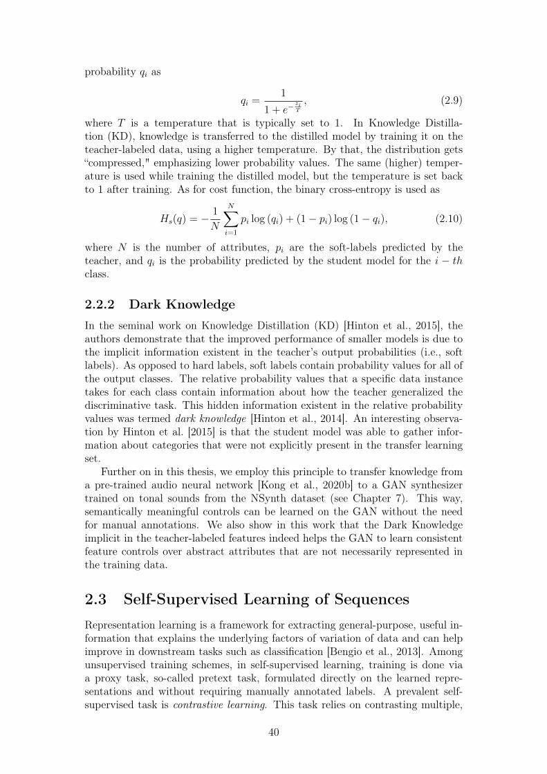
probability qi as

qi =1

1 + e−ziT

, (2.9)

where T is a temperature that is typically set to 1. In Knowledge Distilla-tion (KD), knowledge is transferred to the distilled model by training it on theteacher-labeled data, using a higher temperature. By that, the distribution gets“compressed," emphasizing lower probability values. The same (higher) temper-ature is used while training the distilled model, but the temperature is set backto 1 after training. As for cost function, the binary cross-entropy is used as

Hs(q) = − 1

N

N∑i=1

pi log (qi) + (1− pi) log (1− qi), (2.10)

where N is the number of attributes, pi are the soft-labels predicted by theteacher, and qi is the probability predicted by the student model for the i − thclass.

2.2.2 Dark Knowledge

In the seminal work on Knowledge Distillation (KD) [Hinton et al., 2015], theauthors demonstrate that the improved performance of smaller models is due tothe implicit information existent in the teacher’s output probabilities (i.e., softlabels). As opposed to hard labels, soft labels contain probability values for all ofthe output classes. The relative probability values that a specific data instancetakes for each class contain information about how the teacher generalized thediscriminative task. This hidden information existent in the relative probabilityvalues was termed dark knowledge [Hinton et al., 2014]. An interesting observa-tion by Hinton et al. [2015] is that the student model was able to gather infor-mation about categories that were not explicitly present in the transfer learningset.

Further on in this thesis, we employ this principle to transfer knowledge froma pre-trained audio neural network [Kong et al., 2020b] to a GAN synthesizertrained on tonal sounds from the NSynth dataset (see Chapter 7). This way,semantically meaningful controls can be learned on the GAN without the needfor manual annotations. We also show in this work that the Dark Knowledgeimplicit in the teacher-labeled features indeed helps the GAN to learn consistentfeature controls over abstract attributes that are not necessarily represented inthe training data.

2.3 Self-Supervised Learning of SequencesRepresentation learning is a framework for extracting general-purpose, useful in-formation that explains the underlying factors of variation of data and can helpimprove in downstream tasks such as classification [Bengio et al., 2013]. Amongunsupervised training schemes, in self-supervised learning, training is done viaa proxy task, so-called pretext task, formulated directly on the learned repre-sentations and without requiring manually annotated labels. A prevalent self-supervised task is contrastive learning. This task relies on contrasting multiple,

40

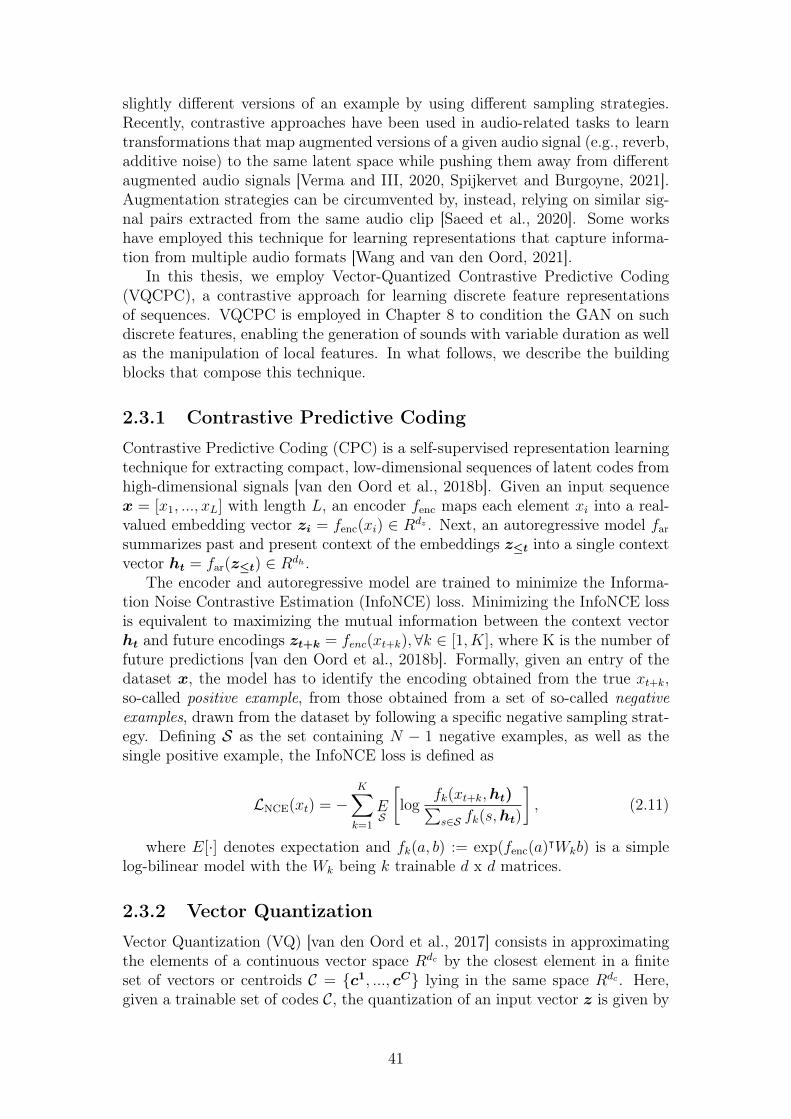
slightly different versions of an example by using different sampling strategies.Recently, contrastive approaches have been used in audio-related tasks to learntransformations that map augmented versions of a given audio signal (e.g., reverb,additive noise) to the same latent space while pushing them away from differentaugmented audio signals [Verma and III, 2020, Spijkervet and Burgoyne, 2021].Augmentation strategies can be circumvented by, instead, relying on similar sig-nal pairs extracted from the same audio clip [Saeed et al., 2020]. Some workshave employed this technique for learning representations that capture informa-tion from multiple audio formats [Wang and van den Oord, 2021].

In this thesis, we employ Vector-Quantized Contrastive Predictive Coding(VQCPC), a contrastive approach for learning discrete feature representationsof sequences. VQCPC is employed in Chapter 8 to condition the GAN on suchdiscrete features, enabling the generation of sounds with variable duration as wellas the manipulation of local features. In what follows, we describe the buildingblocks that compose this technique.

2.3.1 Contrastive Predictive Coding

Contrastive Predictive Coding (CPC) is a self-supervised representation learningtechnique for extracting compact, low-dimensional sequences of latent codes fromhigh-dimensional signals [van den Oord et al., 2018b]. Given an input sequencex = [x1, ..., xL] with length L, an encoder fenc maps each element xi into a real-valued embedding vector zi = fenc(xi) ∈ Rdz . Next, an autoregressive model farsummarizes past and present context of the embeddings z≤t into a single contextvector ht = far(z≤t) ∈ Rdh .

The encoder and autoregressive model are trained to minimize the Informa-tion Noise Contrastive Estimation (InfoNCE) loss. Minimizing the InfoNCE lossis equivalent to maximizing the mutual information between the context vectorht and future encodings zt+k = fenc(xt+k),∀k ∈ [1, K], where K is the number offuture predictions [van den Oord et al., 2018b]. Formally, given an entry of thedataset x, the model has to identify the encoding obtained from the true xt+k,so-called positive example, from those obtained from a set of so-called negativeexamples, drawn from the dataset by following a specific negative sampling strat-egy. Defining S as the set containing N − 1 negative examples, as well as thesingle positive example, the InfoNCE loss is defined as

LNCE(xt) = −K∑k=1

ES

[log

fk(xt+k,ht)∑s∈S fk(s,ht)

], (2.11)

where E[·] denotes expectation and fk(a, b) := exp(fenc(a)ᵀWkb) is a simplelog-bilinear model with the Wk being k trainable d x d matrices.

2.3.2 Vector Quantization

Vector Quantization (VQ) [van den Oord et al., 2017] consists in approximatingthe elements of a continuous vector space Rdc by the closest element in a finiteset of vectors or centroids C = {c1, ..., cC} lying in the same space Rdc . Here,given a trainable set of codes C, the quantization of an input vector z is given by

41

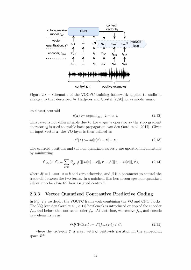
Figure 2.8 – Schematic of the VQCPC training framework applied to audio inanalogy to that described by Hadjeres and Crestel [2020] for symbolic music.

its closest centroidc(z) := argminc∈C||z − c||2. (2.12)

This layer is not differentiable due to the argmin operator so the stop gradientoperator sg is used to enable back-propagation [van den Oord et al., 2017]. Givenan input vector z, the VQ layer is then defined as

zq(z) := sg[c(z)− z] + z. (2.13)

The centroid positions and the non-quantized values z are updated incrementallyby minimizing

LVQ(z, C) =∑c∈C

δczq(z)((||sg[z]− c||2)2 + β(||z − sg[c]||2)2), (2.14)

where δab = 1 ⇐⇒ a = b and zero otherwise, and β is a parameter to control thetrade-off between the two terms. In a nutshell, this loss encourages non-quantizedvalues z to be close to their assigned centroid.

2.3.3 Vector Quantized Contrastive Predictive Coding

In Fig. 2.8 we depict the VQCPC framework combining the VQ and CPC blocks.The VQ [van den Oord et al., 2017] bottleneck is introduced on top of the encoderfenc and before the context encoder far. At test time, we remove far, and encodenew elements xi as

VQCPC(xi) := zq(fenc(xi)) ∈ C, (2.15)

where the codebook C is a set with C centroids partitioning the embeddingspace Rdc .

42

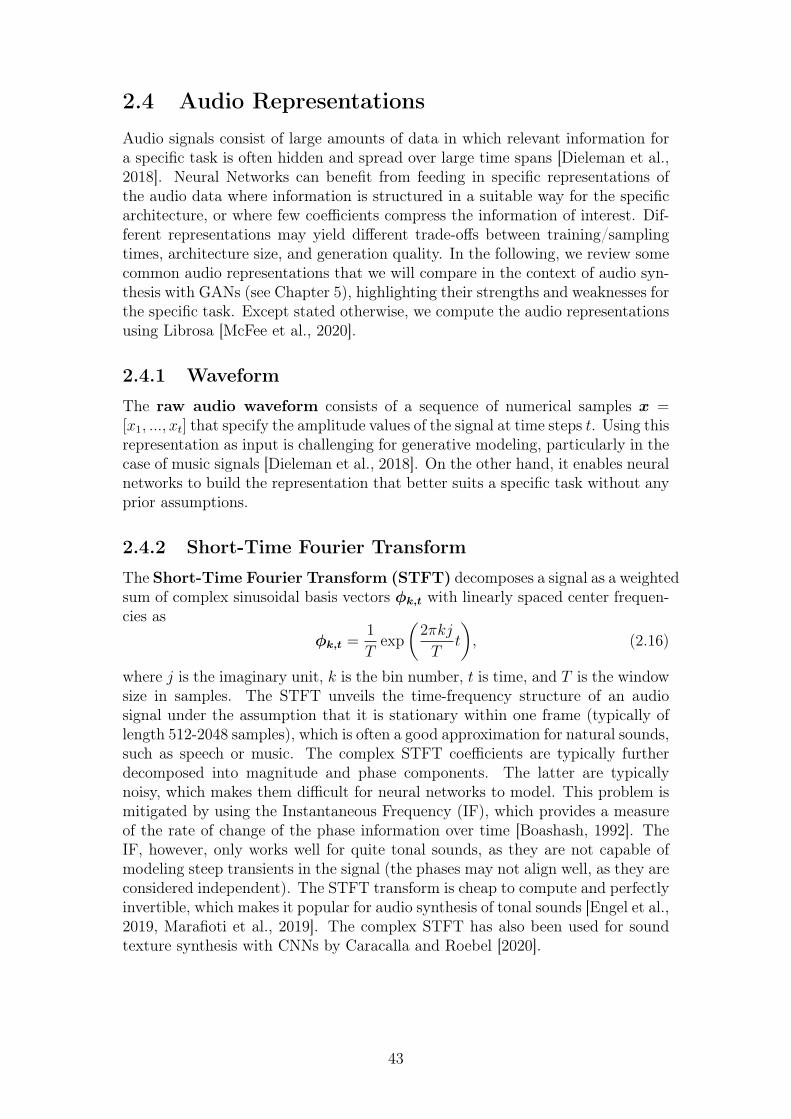
2.4 Audio RepresentationsAudio signals consist of large amounts of data in which relevant information fora specific task is often hidden and spread over large time spans [Dieleman et al.,2018]. Neural Networks can benefit from feeding in specific representations ofthe audio data where information is structured in a suitable way for the specificarchitecture, or where few coefficients compress the information of interest. Dif-ferent representations may yield different trade-offs between training/samplingtimes, architecture size, and generation quality. In the following, we review somecommon audio representations that we will compare in the context of audio syn-thesis with GANs (see Chapter 5), highlighting their strengths and weaknesses forthe specific task. Except stated otherwise, we compute the audio representationsusing Librosa [McFee et al., 2020].

2.4.1 Waveform

The raw audio waveform consists of a sequence of numerical samples x =[x1, ..., xt] that specify the amplitude values of the signal at time steps t. Using thisrepresentation as input is challenging for generative modeling, particularly in thecase of music signals [Dieleman et al., 2018]. On the other hand, it enables neuralnetworks to build the representation that better suits a specific task without anyprior assumptions.

2.4.2 Short-Time Fourier Transform

The Short-Time Fourier Transform (STFT) decomposes a signal as a weightedsum of complex sinusoidal basis vectors φk,t with linearly spaced center frequen-cies as

φk,t =1

Texp

(2πkj

Tt

), (2.16)

where j is the imaginary unit, k is the bin number, t is time, and T is the windowsize in samples. The STFT unveils the time-frequency structure of an audiosignal under the assumption that it is stationary within one frame (typically oflength 512-2048 samples), which is often a good approximation for natural sounds,such as speech or music. The complex STFT coefficients are typically furtherdecomposed into magnitude and phase components. The latter are typicallynoisy, which makes them difficult for neural networks to model. This problem ismitigated by using the Instantaneous Frequency (IF), which provides a measureof the rate of change of the phase information over time [Boashash, 1992]. TheIF, however, only works well for quite tonal sounds, as they are not capable ofmodeling steep transients in the signal (the phases may not align well, as they areconsidered independent). The STFT transform is cheap to compute and perfectlyinvertible, which makes it popular for audio synthesis of tonal sounds [Engel et al.,2019, Marafioti et al., 2019]. The complex STFT has also been used for soundtexture synthesis with CNNs by Caracalla and Roebel [2020].

43

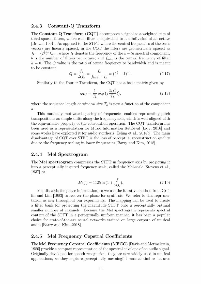
2.4.3 Constant-Q Transform

The Constant-Q Transform (CQT) decomposes a signal as a weighted sum oftonal-spaced filters, where each filter is equivalent to a subdivision of an octave[Brown, 1991]. As opposed to the STFT where the central frequencies of the basisvectors are linearly spaced, in the CQT the filters are geometrically spaced asfk = (2

1b )kfmin, where fk denotes the frequency of the k− th spectral component,

b is the number of filters per octave, and fmin is the central frequency of filterk = 0. The Q value is the ratio of center frequency to bandwidth and is meantto be constant

Q =fk

∆fk=

fkfk+1 − fk

= (21b − 1)−1. (2.17)

Similarly to the Fourier Transform, the CQT has a basis matrix given by

φk,t =1

Tkexp

(j

2πQ

Tkt), (2.18)

where the sequence length or window size Tk is now a function of the componentk.

This musically motivated spacing of frequencies enables representing pitchtranspositions as simple shifts along the frequency axis, which is well-aligned withthe equivariance property of the convolution operation. The CQT transform hasbeen used as a representation for Music Information Retrieval [Lidy, 2016] andsome works have exploited it for audio synthesis [Esling et al., 2018b]. The maindisadvantage of CQT over STFT is the loss of perceptual reconstruction qualitydue to the frequency scaling in lower frequencies [Barry and Kim, 2018].

2.4.4 Mel Spectrogram

The Mel spectrogram compresses the STFT in frequency axis by projecting itinto a perceptually inspired frequency scale, called the Mel-scale [Stevens et al.,1937] as

M(f) = 1125 ln (1 +f

700). (2.19)

Mel discards the phase information, so we use the iterative method from Grif-fin and Lim [1983] to recover the phase for synthesis. We refer to this represen-tation as mel throughout our experiments. The mapping can be used to createa filter bank for projecting the magnitude STFT onto a perceptually optimalsmaller number of channels. Because the Mel spectrogram represents spectralcontent of the STFT in a perceptually uniform manner, it has been a popularchoice for state-of-the-art neural networks trained on large corpora of musicalaudio [Barry and Kim, 2018].

2.4.5 Mel Frequency Cepstral Coefficients

TheMel Frequency Cepstral Coefficients (MFCC) [Davis and Mermelstein,1980] provide a compact representation of the spectral envelope of an audio signal.Originally developed for speech recognition, they are now widely used in musicalapplications, as they capture perceptually meaningful musical timbre features

44

[Ravelli et al., 2010]. For synthesis, we invert MFCC to the Mel scale and useGriffin-Lim algorithm to recover the phase.

45

46

Chapter 3

Related Work

Many works have applied deep generative methods to address general audio syn-thesis. In Chapter 2, we provided a theoretical introduction to each of thesemethods, categorised into exact, approximate, and implicit, depending on theway they estimate the probability distribution of a given training dataset. Fromthe exact family, we highlighted Neural Autoregressive Models (NAMs) and Nor-malizing Flows (NFs), from the approximate methods, we reviewed VariationalAutoencoders (VAEs), and, from the implicit strategies, we described GenerativeAdversarial Networks (GANs). This chapter provides a broad overview of thestate-of-the-art works applying such generative strategies to various audio syn-thesis tasks (see Section 3.1). Special attention is paid to those works focused onmusical audio and the control they offer over the generated sound. We also reviewother audio modeling techniques based on Digital Signal Processing (DSP) andthat, while not relying on deep learning, have been used to study intuitive andcontrollable audio synthesis (see Section 3.2). In Section 3.3, we conclude withsome discussion thereof.

3.1 Neural Audio SynthesizersNeural Audio Synthesizers are generative models that learn from audio data.In this section, we provide an extensive review of the literature on neural audiosynthesis, organized based on the generative principles seen in Chapter 2 (NAMs,NFs, VAEs, and GANs). While there exist many direct applications of thesemethods to audio [van den Oord et al., 2016a, Aouameur et al., 2019, Engelet al., 2019], we will see that many works advocate for distributed solutionscombining various of these techniques, e.g., VAEs and NFs [Kingma et al., 2016],AEs and NAMs [Engel et al., 2017]. Special attention is drawn towards thecontrollability of generative models of audio. Also, we highlight the type of audiosources modeled by each work, the conditional information (if applicable), andthe form of the audio representation.

3.1.1 Controllable Neural Audio Synthesis

One important aspect that we stressed in the introduction of this thesis is that ofintuitive control over the audio synthesis process. Two common strategies existfor achieving controllable generative models: supervised and unsupervised. Su-

47

pervised methods explicitly condition the model on auxiliary information duringtraining. Conditional information is said to be sparse or dense depending on itsamount of information or, in other words, how much of the variance it captures[Dieleman, 2020]. Also, each generative approach supports conditioning differ-ently. Autoregressive models, which operate on a sample-by-sample basis, maybe more inefficient when conditioned on global aspects of the data as informationhas to be repeated at each step in the sequence. GANs, on the contrary, can dealeasily with global properties as they generate the whole piece of data in one pass.

An obvious example of a conditional generative model can be seen in text-to-speech synthesis, where the task of generating realistic speech is conditioned onsome input text information [Shen et al., 2018]. Similarly, singing voice synthe-sizers are generally conditioned on pitch and lyric information [Nishimura et al.,2016, Blaauw and Bonada, 2017]. Neural audio synthesizers of instrument soundscondition on the instrument category and pitch [Engel et al., 2019, 2017, Rocheet al., 2018]. Conditioning is not restricted to symbolic or sparse information(e.g., pitch, words, instrument). Other works use rather dense information andcondition the models on preexisting audio content to drive the generative process.For example, in style transfer tasks, the goal is to take some piece of music in aspecific style (e.g., rock, pop) and transform it into another style while preserv-ing some fundamental content [Huang et al., 2019b, Mor et al., 2018, Cífka et al.,2021]. Other tasks conditioning on dense information are audio enhancement[Michelsanti and Tan, 2017, Biswas and Jia, 2020] or spectrogram inversion [Ku-mar et al., 2019]. While supervised methods rely on preexisting information tocondition the model, unsupervised methods employ feature learning mechanismsto discover important factors of variations of the data autonomously. At testtime, such learned features can potentially be used to guide the generation pro-cess. Some of the most successful applications of unsupervised feature learning forcontrollable generation can be found in face image synthesis tasks, where GANscan autonomously learn high-level attributes (e.g., pose, identity) separately fromstochastic variation (e.g., hair) [Karras et al., 2018].

3.1.2 Neural Autoregressive Models

Neural Autoregressive Models (NAMs) are probably the most popular approachfor building generative neural networks of audio. In the following sections wereview some of the most important works applying NAMs to audio. First wefocus on WaveNet and other popular works down the line which are based oncausal convolutions. Next, we revise some other approaches that use differentoperations (e.g., recurrent, attention). Last, we mention some hybrid approachesthat introduce autoregressive models as part of larger distributed systems. Thisenables, for example, to combine the robustness of autoregressive modeling withthe latent space control that autoencoders offer.

WaveNet-like Architectures

The recently-developed WaveNet architecture [van den Oord et al., 2016a] is oneof the most important architectures used for realistic speech synthesis and themost influential work in autoregressive models for audio generation in general.Inspired by other works in image [van den Oord et al., 2016c], it operates directly

48

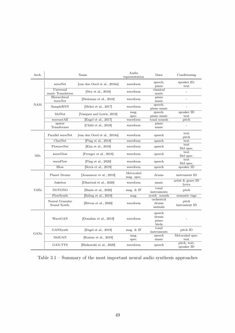
Arch. Name Audiorepresentation Data Conditioning

waveNet [van den Oord et al., 2016a] waveform speech,piano

speaker ID,text

Universalmusic Translation [Mor et al., 2018] waveform classical

music -

NAM

HierarchicalwaveNet [Dieleman et al., 2018] waveform piano

music -

SampleRNN [Mehri et al., 2017] waveform speech,piano music -

MelNet [Vasquez and Lewis, 2019] mag.spec.

speech,piano music

speaker IDtext

wavenetAE [Engel et al., 2017] waveform tonal sounds pitchsparse

Transformer [Child et al., 2019] waveform pianomusic -

Parallel waveNet [van den Oord et al., 2018a] waveform speech textpitch

ClariNet [Ping et al., 2018] waveform speech text

FlowaveNet [Kim et al., 2018] waveform speech textMel spec.

NFs waveGlow [Prenger et al., 2018] waveform speech textMel spec.

waveFlow [Ping et al., 2020] waveform speech textMel spec.

Blow [Serrà et al., 2019] waveform speech speaker ID

Planet Drums [Aouameur et al., 2019] Mel-scaledmag. spec. drums instrument ID

Jukebox [Dhariwal et al., 2020] waveform music artist & genre IDlyrics

VAEs NOTONO [Bazin et al., 2020] mag. & IF tonalinstruments pitch

FlowSynth [Esling et al., 2019] mag. synth. sounds semantic tags

Neural GranularSound Synth. [Bitton et al., 2020] waveform

orchestraldrumsanimals

pitchinstrument ID

WaveGAN [Donahue et al., 2019] waveform

speechdrumspianobirds

-

GANsGANSynth [Engel et al., 2019] mag. & IF tonal

instruments pitch ID

MelGAN [Kumar et al., 2019] mag.spec.

speechmusic

Mel-scaled spec.text

GAN-TTS [Binkowski et al., 2020] waveform speech pitch, text,speaker ID

Table 3.1 – Summary of the most important neural audio synthesis approaches

49

on the raw audio by modelling the probability of a waveform xxx = [x1, ..., xT , fac-torised as a product of conditional probabilities (see Sec. 2.1.1). The architectureis built as a stack of Dilated Causal Convolutional layers. The filters in each con-volutional layer are applied over an area larger than its length by skipping inputvalues with a certain step or dilation. At each layer in the network, the dilationfactor is doubled, allowing the network to grow its receptive field (i.e., the regionof the sensory space that the network observes) exponentially with depth whilepreserving the number of computations. This dilation enables the model to oper-ate on a coarser scale, capturing longer-term audio dependencies while preservingthe information’s resolution throughout the network. The output layer consists ofa Softmax activation unit that models a categorical distribution over 256 possibleamplitude values. Given an additional conditioning input, the authors can guidethe generation of audio with certain characteristics and at different scales. Forexample, when applying WaveNet in speech generation, they can impose globalcharacteristics on the speaker, such as its identity, or local characteristics, such asthe phoneme to be synthesized, by conditioning the network on text information.During training, every causal convolutional layer can process its input in par-allel, making these architectures faster than RNNs, which can only be updatedsequentially. At generation time, however, the waveform has to be synthesizedsequentially as xt must be sampled first to obtain xi>t. Due to this fact, real-timesynthesis is challenging, in particular for music applications [van den Oord et al.,2018a].

Many efforts have been made to improve WaveNet’s time and computationefficiency. Fast WaveNet [Paine et al., 2016] reduces the complexity of the al-gorithm from O(2L) to O(L) time (being L the network’s number of layers) bystoring previous convolution calculations in order to remove redundant opera-tions. This approach requires the use of smaller networks, impacting the qualityof the synthesized audio severely. In Sec. 3.1.4 we review a more recent approach,based on NFs, that introduces Probability Density Distillation [van den Oordet al., 2018a], a method for transferring knowledge from pre-trained WaveNet toa smaller NF with no significant degradation in quality. The resulting system iscapable of generating high-quality speech and in real-time.

The use of WaveNet in speech, singing voice, and music synthesis has beenpredominant. As we will see later in this section, most of these works applyWaveNet as a waveform synthesizing building block, part of a larger distributedparametric system [Gibiansky et al., 2017, Ping et al., 2017, Shen et al., 2018,Roebel and Bous, 2021] or following an encoder-decoder architecture to providemeans of control through the latent space [Engel et al., 2017].

Non-Convolutional Approaches

Neural autoregressive models may employ operations other than dilated con-volutions such as recurrent connections or attention mechanisms. SampleRNN[Mehri et al., 2017] uses multiple RNNs stacked on top of each other, where eachblock in the stack operates at a different rate. Higher-level RNNs update lessfrequently, which means they can more easily capture long-range data dependen-cies and learn high-level features. Conversely, lower layers in the stack runningat a faster rate capture local, fast-varying dependencies of the data (e.g., pitch,timbre, envelope).

50

We mentioned in Section 2.1.1 that autoregressive models, while naturallyfitting the sequential scheme of the audio waveform, can be used on other audiorepresentations. Using spectrograms, for example, one can easily increase thereceptive field of a model (i.e., spectrograms condense the time information ofa whole analysis frame in each frequency bin), simplifying the task of capturingglobal structure in comparison to other autoregressive approaches that work withaudio in the time domain. MelNet [Vasquez and Lewis, 2019] is an RNN-basedautoregressive model that operates on high-resolution time-frequency magnitudespectrograms, capturing long-range dependencies of the data. It combines a fine-grained autoregressive model and a multi-scale generation procedure to capturestructure in a coarse-to-fine-grain manner jointly. The autoregressive model fac-torizes the distribution over both the time and frequency dimensions. Thanks tothe time-condensed representation of magnitude spectrograms, coupled with thepower of autoregressive models, MelNet achieves highly expressive and end-to-endunconditional audio generation for speech and music data.

Plain recurrent blocks tend to be slow during training and have difficultylearning dependencies between distant elements from the sequence. Introducingattention mechanisms allows an autoregressive model to access any part of thepreviously generated output at every step of generation [Vaswani et al., 2017].Works on audio have used attention as part of an encoder-decoder architectureto pass relevant information from a latent space to a decoder generating, e.g.,vocoder parameters [Sotelo et al., 2017], magnitude spectrograms [Wang et al.,2017] or Mel-scaled spectrogram representations [Shen et al., 2018]. Continua-tions of these works were able to generate prosodic speech by conditioning theattention layers on emotion labels [Lee et al., 2017b] as well as to synthesizespeech for multiple speakers [Ping et al., 2017]. Other approaches such as theTransformer [Vaswani et al., 2017, Shaw et al., 2018], abandoned the traditionalencoder-decoder configuration and adopted architectures based solely on atten-tion mechanisms. These architectures have been successfully applied to symbolicmusic [Huang et al., 2019a] and, with the introduction of sparsity, to audio [Childet al., 2019], making it possible to generate minute-long music with rich structureat multiple scales.

Hybrid approaches

A downside of purely autoregressive models is that they do not explicitly producelatent representations of the data, limiting the extent to which they can be con-trolled at generation time. However, it is possible to combine an autoregressivesequence generation model with an encoder-decoder architecture [Engel et al.,2017, Mor et al., 2018, Chorowski et al., 2019]. In these works, an encoder readsa sequence of raw audio samples or feature vectors and extracts a sequence oflatent representations. The decoder reconstructs the utterance by conditioning aWaveNet network on these latent representations and on additional features (e.g.,pitch [Engel et al., 2017], speaker embedding [Chorowski et al., 2019]) to makethe models invariant to specific feature-dependent information. The WaveNetAutoencoder [Engel et al., 2017] yields a pitch-independent timbre latent spacewhere instruments can be morphed together through interpolation, and new typesof sounds can be created that are realistic and expressive. Another work focusedon musical audio style transfer uses WaveNet-like autoencoders to transform the

51

timbre of some input audio to target a specific style [Mor et al., 2018]. The ar-chitecture follows a single-encoder multi-decoder framework with a shared latentspace, enforcing the network to learn a style-invariant latent representation, andeach decoder is therefore responsible for conferring sound style-specific character-istics.

Most of the work in speech [Arik et al., 2017, Gibiansky et al., 2017, Pinget al., 2017, Shen et al., 2018] incorporated an optimized version of WaveNet asa vocoder model for reconstructing speech audio from linguistic features and f0[Arik et al., 2017], linear-scaled log-magnitude spectrograms [Gibiansky et al.,2017] or Mel-scaled spectrograms [Ping et al., 2017], being this last version theone that yields the best performance and a more compact representation of theconditioning audio. Tacotron 2 [Shen et al., 2018] follows the same approach andintroduces a WaveNet vocoder as an improvement of the Griffin-Lim reconstruc-tion module used in Tacotron [Wang et al., 2017]. Tacotron 2 yields some of themost human natural-sounding reconstructions. Similar techniques use WaveNetas part of a distributed system for singing voice synthesis [Blaauw and Bonada,2017]. These works train WaveNet on features produced by a parametric vocoderthat separates the influence of pitch and timbre. This separation allows to mod-ify pitch to match any target melody conveniently, facilitates training on reduceddataset sizes, and significantly improves training and generation times.

3.1.3 Variational Autoencoders

Variational Autoencoders (VAE) [Kingma and Welling, 2014] are one of the mostpopular strategies for generative modeling. One of the main attractive proper-ties behind VAEs is their capability to map data into a structured latent spacethat captures fundamental features. The possibility of controlling the generativeprocess through such a latent space makes them an interesting asset in musicmodeling. Various successful works employ VAEs in symbolic representations[Roberts et al., 2017, Brunner et al., 2018a]. In audio, most initial works weretailored towards synthesis and transformation of speech [Blaauw and Bonada,2016, Hsu et al., 2017]. Even though the latent space of VAEs tends to self-organize according to fundamental dependencies in the data, these can still bedifficult to interpret. Some works in music data focused on regularizing the latentspace of VAEs to accommodate perceptual distances collected from timbre studies[Esling et al., 2018a, Roche, 2020], and synthesize from such latent space audiothat matches a semantically meaningful target descriptor [Esling et al., 2018b].The original VAE formulation, where the inference network is used to parametrizea normal distribution (see Sec. 2.1.3), yields blurred generations [Huang et al.,2018]. Some works use Maximum Mean Discrepancy (MMD) distance instead ofDKL(qφ(z|x)||pθ(z)) 2.4 to alleviate this problem. This approach has been suc-cessfully applied to synthesize percussive sounds, enabling to interpolate betweena wide variety of instruments [Aouameur et al., 2019]. As we will see further onin this section, some other work implicitly imposes the prior distribution by usingan adversarial loss in the latent space [Bitton et al., 2019]. Other works used twoVAEs to implement a granular synthesizer [Bitton et al., 2020]: one that encodesgrain series into compressed codes and a second VAE learning combinations ofcodes to define paths in the latent space of the first VAE. Some other interesting

52

applications of VAEs can encode pre-existing multi-track music material into anintuitive two-dimensional latent space and, from this, generate bass lines fittingthe provided music content [Grachten et al., 2020]. A novel application of VAEsin combination with Normalizing Flows (NFs) can map the learned latent spaceof the VAE to parameters of a synthesizer [Esling et al., 2019]. This formulationenables a single model to perform high-fidelity audio synthesis and automaticparameter inference, macro-control learning, and audio-based preset exploration.

Another problem when generating high-quality audio with VAEs is the poste-rior collapse, by which robust decoding architectures such as WaveNet, may endup ignoring the latent codes. Some techniques discretize the latent space throughparametrization of the posterior distribution using Vector Quantization (VQ),enabling the prior to be learned instead of imposed [van den Oord et al., 2017].This architecture has shown remarkable results in tasks such as speech genera-tion and speaker translation [Chorowski et al., 2019]. Following this line, Jukebox[Dhariwal et al., 2020] is a multi-scale VQ-VAE combined with Transformers thatgenerates minute-long music with a singing voice in the raw audio domain. Itallows conditioning on the artist, genre, and lyric information to steer the musicaland vocal style of the generated content. This work sets a milestone in modelinglong-term structure from large-scale music audio datasets and demonstrates thepower of deep learning to model creative tasks. Other applications of VQ-VAEsinclude in-painting-based synthesis of tonal instruments [Bazin et al., 2020] orone-shot timbre style transfer [Cífka et al., 2021].

3.1.4 Normalizing Flows

Normalizing Flows (NFs) have recently become popular in the speech synthe-sis community. In Section 2.1.2 we studied how Normalizing Flows (NF) canbe used to learn rich and flexible posteriors in DL-based variational inferenceby using neural networks implementing invertible transformations. One of themain shortcomings of NFs is their requirement to have the same input and la-tent dimensions, challenging the modeling of high-dimensional data as is the casein audio signals. A specific type of NF known as Inverse Autoregressive Flow(IAF) [Kingma et al., 2016] scales well to high-dimensional data by implementingthe invertible transformation as an autoregressive neural network. The increasedefficiency of IAFs has been used in audio to accelerate WaveNet-based speechsynthesis to 20x faster than real-time [van den Oord et al., 2018a]. This workintroduces a new method coined Probability Density Distillation, which allowstraining an IAF from a pre-trained teacher WaveNet with no significant differ-ence in quality and enabling parallel sampling. However, this two-stage trainingpipeline is cumbersome and requires highly regularized training to avoid modefailure in the student. Subsequent works combine insights from Glow [Kingma andDhariwal, 2018], and WaveNet [van den Oord et al., 2016a] to design flow-basedmodels that provide fast, efficient, and high-quality speech generation withoutthe need of two-stage training schemes nor additional auxiliary loss terms [Kimet al., 2018, Prenger et al., 2018, Ping et al., 2020]. Some works down this lineemployed similar flow-based architectures for non-parallel voice conversion [Serràet al., 2019]. Applications of NFs to musical audio synthesis are scarce. As wehave seen, some works have used flows in combination with VAEs to learn in-

53

vertible mappings between the VAE’s latent space and a synthesizer’s parameterspace [Esling et al., 2019].

3.1.5 Generative Adversarial Networks

Generative Adversarial Networks (GANs) [Goodfellow et al., 2014] have beenshown successful in various computer vision tasks such as image inpainting [Den-ton et al., 2016], domain translation and style transfer [Zhu et al., 2017, Choi et al.,2018, Liu and Tuzel] or high-fidelity image generation [Gulrajani et al., 2017, Chenet al., 2016b, Karras et al., 2018]. Taking inspiration from these works, applica-tions of GANs to audio synthesis have mainly focused on speech tasks [Saito et al.,2018, Kaneko and Kameoka, 2017, Huang et al., 2019b, Binkowski et al., 2020,Kong et al., 2020a, Kumar et al., 2019, Yamamoto et al., 2020]. Initial worksdemonstrated that adversarial training could convert one speaker into anotherwhile preserving the linguistic content [Kaneko and Kameoka, 2017] or synthesiz-ing realistic speech from text [Saito et al., 2018]. Novel cross-modal applicationsuse conditional GANs to generate sound from image information and vice-versa[Chen et al., 2017, Iashin and Rahtu, 2021]. GANs have been used for symbolicmusic generation using a Recurrent Neural Network generator [Lee et al., 2017a]or in music genre transfer using cycle-consistent architectures [Brunner et al.,2018b]. The first application to musical audio synthesis was WaveGAN [Donahueet al., 2019]. Although it did not match autoregressive baselines such as WaveNet[van den Oord et al., 2016a] in terms of audio quality, it could generate pianoand drum sounds in a short amount of time and in an entirely unconditionalway. Recent work along the line of WaveGAN has achieved some promising re-sults in footstep sound synthesis [Comunità et al., 2021]. General improvementsin the stabilization and training of GANs [Karras et al., 2017, Gulrajani et al.,2017, Salimans et al., 2016] enabled GANSynth [Engel et al., 2019] to outperformWaveNet baselines on the task of audio synthesis of musical notes using sparsepitch conditioning labels. GANSynth follows the principle of Progressive Growingof GANs (PGAN) [Karras et al., 2017], where a generative network, composedof convolutional and up-sampling blocks, is built on the fly while training (seeSection 2.1.4). Follow-up works building on GANSynth applied similar architec-tures to conditional drum sound synthesis using different metadata [Nistal et al.,2020, Drysdale et al., 2020]. DrumGAN [Nistal et al., 2020] synthesizes a varietyof drum sounds based on high-level input features describing timbre (e.g., boomi-ness, roughness, sharpness). Given their mode-seeking behaviour (see Sec. 2.1.4),GANs have been popular in densely conditioned tasks such as Mel-spectrograminversion for speech [Kumar et al., 2019] or singing voice synthesis [Chen et al.,2021], audio domain adaptation [Hosseini-Asl et al., 2018, Michelsanti and Tan,2017] or audio enhancement [Biswas and Jia, 2020]. Some works introduce adver-sarial objectives into the VAE training scheme to synthesize Mel-spectrograms oforchestral instruments given a note class and some latent vector capturing styleparameters [Bitton et al., 2019]. While GANs often require large amounts of datato learn some specific task, recently, patch-based GANs were shown capable oflearning from one single image example, capturing its internal distribution, andenabling to generate variations from it [Shaham et al., 2019]. This approach hasbeen successfully translated to the audio domain for sound effect, speech, or mu-

54

sic generation [Barahona-Ríos and Collins, 2021, Greshler et al., 2021]. A recentwork proposes a combination of the autoregressive and adversarial schemes bysampling large chunks of the waveform during each autoregressive forward pass,bringing together the fast generation capabilities of GANs with the benefits ofthe autoregressive inductive bias [Morrison et al., 2021].

3.2 Audio Synthesis Prior the Deep Learning EraThe interest of humans in crafting machines that can generate sounds and musicdates back to at least the 19th century when Ada Lovelace anticipated the era ofcomputer music [Fuegi and Francis, 2015] and the first generation of ElectronicMusical Instruments (EMI) appeared [Crab, 2016]. A wide variety of sound mod-els have been proposed since then. These can be categorized into abstract, spec-tral, physical, or based on processed recordings, depending on how they modelsound [Smith, 1991]. Essentially, most of these methods start from some fun-damental waveforms, which are combined and transformed in various ways toproduce different sounds. Techniques differ in the shape of such fundamentalwaveforms and the way these are processed to form richer sounds. Also, eachmethod exhibits characteristics that could make it preferable over others depend-ing on the specific musical purposes. In this section, we briefly overview some ofthese modeling strategies and research aimed at devising semantically intuitiveinterfaces for their control. For an in-depth review of these works we refer thereader to Roads et al. [1997], Smith [a], Miranda [2002].

3.2.1 Abstract Models

Abstract methods such as Frequency Modulation (FM) [Chowning, 1973], imple-mented in the famous Yamaha DX7, use algorithmic procedures or conceptualmathematical formulations to model sound [Roads et al., 1997]. As a result,the parameters offered by these types of synthesis techniques do not have a directphysical or perceptual meaning and fail to precisely model existing natural sounds[Miranda, 2002]. However, they have been highly appreciated due to their lowcomputational and memory requirements as well as their rich timbre capabilities,with just a few parameters, that allow synthesizing sounds that would otherwisebe impossible to generate through physical means [Kleimola, 2013]. Today, whileabstract methods have lost some of their original prominence and are consideredobsolete from a research perspective [Serra, 2007], we can find them as a buildingblock of many commercial applications based on other modeling principles (e.g.,subtractive1, wavetable2).

3.2.2 Spectral Models

Spectral models synthesize sound by characterizing its spectral content followingFourier theory. The earliest and simplest form of spectral modeling is additivesynthesis, which forms sound as a sum of discrete sinusoidal components mod-ulated by time-varying amplitude and frequency envelopes [Smith, b]. While

1https://www.waves.com/plugins/flow-motion-fm-synth2https://www.reasonstudios.com/shop/rack-extension/wtfm-wavetable-fm-synthesizer/

55

their parameters are closer to human perception than other strategies [Serraet al., 2007], these require many components to properly model rich sounds,which makes them computationally expensive [Miranda, 2002]. Alternative tech-niques introduce a time-varying filtered noise to model stochastic components inthe sound and also allow for analysis of existing audio signals [Serra and Smith,1990].

Another spectral modeling strategy, and one of the most popular techniquesimplemented in commercial synthesizers (e.g., Minimoog Model D, Roland TR-808), is subtractive synthesis. Loosely categorized as a source-filter modelingtechnique, subtractive synthesis can be seen as the inverse process to additivesynthesis, where rich broadband signals such as square, saw-tooth, pulses, ornoise are filtered to remove undesired frequency components [Roads et al., 1997].While their controls are much less numerous than for additive synthesis and arecomputationally cheap, they are less flexible and fail to capture faithfully manyacoustic instruments [Miranda, 2002].

3.2.3 Physical Models

Physical models can emulate acoustic instruments by mathematically reproducingin a computer their mechanical behavior and solving their associated differentialequations to produce sound [Miranda, 2002]. These techniques can synthesizerealistic sounding instruments and have the benefit of providing intuitive con-trols responding to physical properties of the acoustic source (e.g., the stiffness,tension) or the excitation signal (e.g., strength, friction) [Roads et al., 1997].However, they are computationally expensive and, analogously to their acousticcounterparts, they can only generate a limited variety of timbre. Today, effortsare focused on providing more flexible approaches based on a combination of el-ementary model blocks, physical modeling based on data analysis, or its use incombination with spectral methods [Serra et al., 2007, Smith, a].

3.2.4 Processed Recording

Early examples of sound creation from processed recordings were based on trans-forming and looping short snippets of sounds recorded in tapes to create novelsound compositions. This technique was pioneered in music by many technolo-gists, and music futurists such as Edgard Varèse and Pierre Schaeffer in MusiqueConcrète [Miranda, 2002]. With the increasing storage and computing capabili-ties of computers, these sample-based techniques evolved into more sophisticatedones such as granular synthesis, producing sounds based on short, time-varyingportions of sampled sounds, so-called grains [Roads et al., 1997]. From a moregeneral perspective, wavetable techniques allowed to repeatedly playback arbi-trary wave shapes stored in a lookup table [Smith, 1991]. More recently, andwith the ever-growing availability of audio datasets, concatenative synthesis in-troduced the notion of analysis to assemble the desired sound according to somepredefined sound descriptors or by analysis of an existing sound [Schwarz, 2007].A prominent example of these is Vocaloid,3 a real-time singing voice synthesizer

3https://www.vocaloid.com/en/

56

that can be controlled with some input text and timbre features. Today, many ad-vanced synthesizers are based on samplers such as Native Instruments’ Kontakt4and Steinberg’s HALion,5 achieving some of the most detailed and accurate em-ulations of acoustic instruments, where no other synthesis technique is capable ofthe same levels of realism. Nevertheless, these techniques generally do not allowfor a rich manipulation or require large amounts of data to generate expressivesounds [Smith, 2004].

3.2.5 Knowledge-driven Controllable Audio Synthesis

Audio synthesizers have given birth to a new paradigm for producing soundswhere no a-priory limitation exists on the kind of sounds that can be produced orhow we can interact with them. In contrast, acoustic instruments are limited bytheir specific physical characteristics constraining the sounds they can produceand the means of interaction. However, acoustic instruments offer a very intu-itive interface where the interaction mechanics are directly related to high-levelproperties of the sound, i.e., the pressure of the bow in a violin is directly relatedto the intensity of the produced sound. A question in synthesizers, therefore, ishow to devise means of control that are suitable for the synthesis algorithm insuch a way for actions and expectations to be consistent [Roads et al., 1997].

As computing capabilities became more powerful during the 90s and early2000s, new research directions appeared related to intuitive control of synthe-sizers where perceptual and cognitive aspects are taken into account in order tosteer the sound synthesis process [Ystad et al., 2019]. In other words, these worksstudied how to map a specific control signal (e.g., gestures [Camurri et al., 2000],perceptual attributes [Aramaki et al., 2011a]) into the synthesizer’s parameters.To this end, perceptual and cognitive studies were carried out to understand theprinciples of how a sound is perceived and its relationship to specific acoustic fea-tures present in the signal, so-called invariants, that can be identified from anal-ysis. Identifying such signal invariants makes it possible to propose perceptualcontrol over the sound synthesis processes that enable direct, evocative control ofsuch perceptual properties. Along this line, some works have attempted to drivethe physical synthesis of environmental sounds such as rain, waves, wind, and firebased on semantic labels, gestures, or drawings [Aramaki et al., 2011b]. Otherworks can derive intuitive perceptual controls on synthesizers of impact soundsby careful study of their acoustic features in consonance with human-annotatedcategories of materials [Aramaki et al., 2006, 2011a]. By considering such re-lationships, a synthesizer can then be designed to control the acoustic featuresfound to correlate with the annotated categories. This process is shown to offermanipulation of intuitive parameters responding to the material label (i.e., Wood,Metal, or Glass). Physical and spectral models have been combined to synthesizeflute sounds based on simulation of the wave propagation in the medium and byusing deterministic plus stochastic decomposition to control independent compo-nents [Ystad, 1998]. The authors can obtain a gesture-driven interface to controlthe proposed model by equipping a flute with sensors. Acoustic invariants relatedto the evocation of continuous interacting solids such as rubbing, scratching, and

4https://www.native-instruments.com/en/products/komplete/samplers/kontakt-6/5https://www.steinberg.net/vst-instruments/halion/

57

rolling were also identified and used for sound synthesis purposes [Conan et al.,2014]. A synthesizer was developed where the actions (e.g., from rolling to slip-ping) and the properties of the acoustic source (shape, size, and material) couldbe controlled continuously over time [Pruvost et al., 2015]. Extensions of theseworks propose a cross-synthesis approach to modify the intrinsic properties of agiven sound texture to evoke a particular interaction (rolling or rubbing) in a wayto create sonic metaphors [Conan, 2014]. A broad perspective of this research isfurther described by Ystad et al. [2019].

3.3 DiscussionThis chapter reviewed works for synthesizing audio using deep learning and, lessextensively, techniques based on traditional signal processing methods, which aredriven by expert knowledge. Here we extend the discussion in Chapter 2, on thebenefits of each deep generative modeling technique, by taking into considerationthe specific advancements in neural audio synthesis and by contrasting them withthose methods employing expert knowledge. Following, we highlight some of themost relevant aspects of the works reviewed in this chapter.

• Expert vs. DL-driven audio synthesis. Many expert-driven synthe-sis methods have been proposed, each offering specific manipulation andsound capabilities [Smith, 1991]. While these can generate a wide varietyof timbres, many complex natural sounds are still not faithfully modeledby these techniques, imposing the need for heavy physical models or data-hungry corpus-based synthesis techniques [Roads et al., 1997]. Neural audiosynthesizers, on the contrary, and Generative Adversarial Networks (GANs)specifically, have been shown to model a great variety of sound sources rang-ing from sound effects to music and speech and using general formulations[Barahona-Ríos and Collins, 2021, Engel et al., 2019, Morrison et al., 2021].Also, as opposed to expert systems [Ystad, 1998], GANs can be controlledbased on abstract descriptors without requiring a principled understandingof the perceptual or timbral properties of the sound and their correspon-dence to feature invariants [Engel et al., 2019]. However, a consequence ofthis is that DL models tend to behave as black boxes whose parameters aredifficult to interpret, whereas expert systems are built upon well-establishedrules and understanding.

• Conditioning & Control. Many works have successfully implementedconditional models of audio to allow some degree of control over the gen-erative process [Engel et al., 2019, 2017, Aouameur et al., 2019]. Modelscan be conditioned on sparse, categorical data, for example, to choose aspeaker identity in speech synthesis [van den Oord et al., 2016a, Vasquezand Lewis, 2019] or an instrument in sound synthesis [Aouameur et al.,2019]. Other works have conditioned the model on rather dense informa-tion, such as spectral information, to constrain some target domain featuresin style transfer [Mor et al., 2018] or in Mel-spectrogram inversion [Kumaret al., 2019]. Autoregressive models of audio, such as WaveNet [van denOord et al., 2016a], do not directly offer a latent space that can be ma-nipulated, and their hidden layers are not regularized to follow any prior

58

distribution, which makes them difficult to control without external condi-tioning. Therefore, many works have made use of WaveNet-like blocks inan encoder-decoder fashion to allow encoding and manipulation of soundsin a latent space [Engel et al., 2017]. Variational Autoencoders (VAEs) andNormalizing Flows (NFs) naturally provide encoders that capture funda-mental aspects of the data and that allow encoder sounds, although thesecan often be hard to effectively condition due to their specific inductive bias[Esling et al., 2019]. GANs have no encoder at all, yet they can be easilyconditioned by just concatenating arbitrary external information to theirlatent noise vectors [Engel et al., 2019].

• Inference and synthesis efficiency. One of the main shortcomings ofNeural Autoregressive Models (NAMs) is their slow generation time due totheir inherent sequential generation scheme [van den Oord et al., 2016a].While methods have been proposed to speed up audio generation in au-toregressive models, these are generally based on cumbersome two-stagetraining schemes or careful architecture designs using flows [van den Oordet al., 2018a, Kim et al., 2018]. GANs, however, can generate full audiosamples in a single forward pass much faster than NAMs. While NFs andVAEs can also be fast, the former tend to require rather deep and inefficientnetworks due to the invertibility constraint, or, in the latter, they tend toproduce blurred, lower-quality samples than other generative strategies.

• Sample quality and diversity. NAMs and GANs have the advantageof generating high-quality audio fidelity with relatively simple networks.While VAEs have traditionally produced worse quality than other genera-tive models, recent works introduce vector-quantization and autoregressiveblocks, achieving impressive audio quality and diversity at the expense ofgeneration time [Dhariwal et al., 2020]. Although GANs lack the same de-gree of diversity as other models due to their mode-seeking nature, theycan generate audio much faster and obtain extremely good sample quality.

59

60

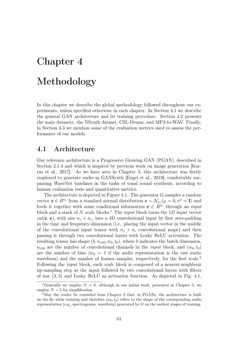
Chapter 4

Methodology

In this chapter we describe the global methodology followed throughout our ex-periments, unless specified otherwise in each chapter. In Section 4.1 we describethe general GAN architecture and its training procedure. Section 4.2 presentsthe main datasets: the NSynth dataset, CSL-Drums, and MP3-to-WAV. Finally,in Section 4.3 we mention some of the evaluation metrics used to assess the per-formance of our models.

4.1 ArchitectureOur reference architecture is a Progressive Growing GAN (PGAN), described inSection 2.1.4 and which is inspired by previous work on image generation [Kar-ras et al., 2017]. As we have seen in Chapter 3, this architecture was firstlyemployed to generate audio in GANSynth [Engel et al., 2019], comfortably sur-passing WaveNet baselines in the tasks of tonal sound synthesis, according tohuman evaluation tests and quantitative metrics.

The architecture is depicted in Figure 4.1. The generator G samples a randomvector zzz ∈ Rnz from a standard normal distribution zzz ∼ Nnz(µ = 0, σ2 = I) andfeeds it together with some conditional information ccc ∈ Rnc through an inputblock and a stack of N scale blocks.1 The input block turns the 1D input vectorcat(zzz, ccc), with size nz + nc, into a 4D convolutional input by first zero-paddingin the time and frequency-dimension (i.e., placing the input vector in the middleof the convolutional input tensor with nz + nc convolutional maps) and thenpassing it through two convolutional layers with Leaky ReLU activation. Theresulting tensor has shape (b, nch0, w0, t0), where b indicates the batch dimension,nch0 are the number of convolutional channels in the input block, and (w0, t0)are the number of bins (w0 = 1 if the audio representation is the raw audiowaveform) and the number of frames/samples, respectively, for the first scale.2Following the input block, each scale block is composed of a nearest-neighbourup-sampling step at the input followed by two convolutional layers with filtersof size (3, 3) and Leaky ReLU as activation function. As depicted in Fig. 4.1,

1Generally we employ N = 6, although in our initial work, presented in Chapter 5, weemploy N = 5 for simplification.

2May the reader be reminded from Chapter 2 that, in PGANs, the architecture is builton the fly while training and therefore (w0, t0) refers to the shape of the corresponding audiorepresentation (e.g., spectrograms, waveform) generated by G on the earliest stages of training.

61

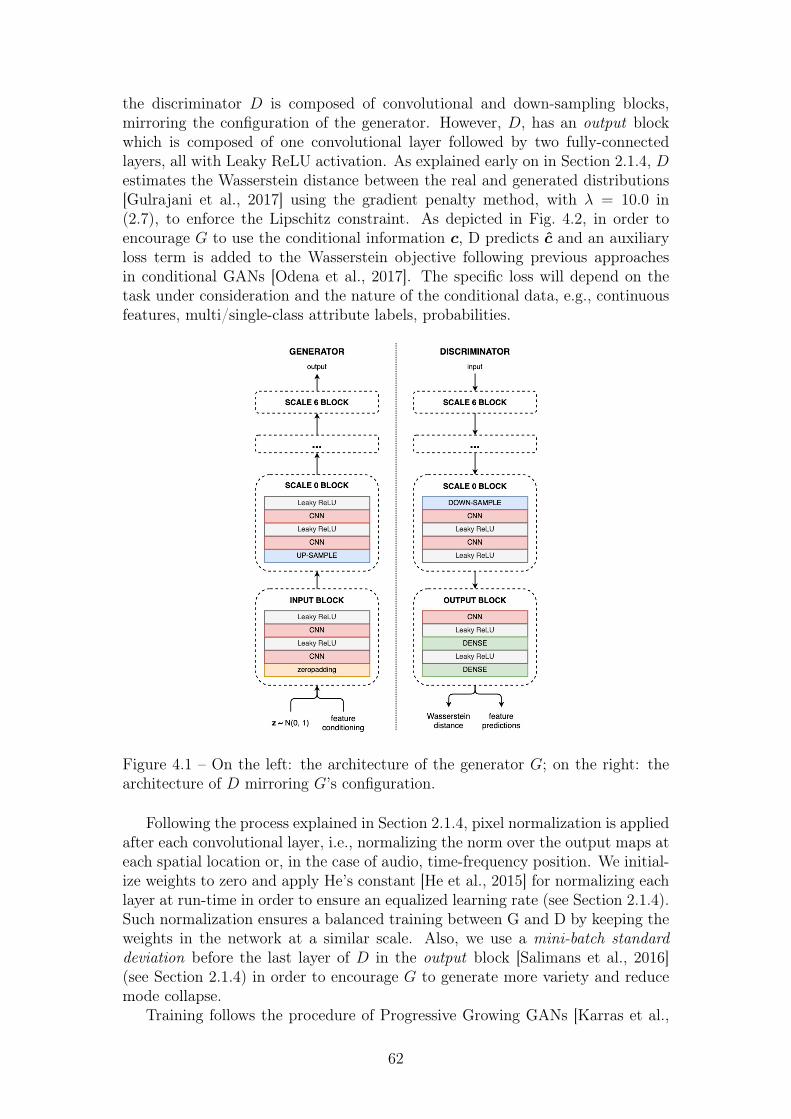
the discriminator D is composed of convolutional and down-sampling blocks,mirroring the configuration of the generator. However, D, has an output blockwhich is composed of one convolutional layer followed by two fully-connectedlayers, all with Leaky ReLU activation. As explained early on in Section 2.1.4, Destimates the Wasserstein distance between the real and generated distributions[Gulrajani et al., 2017] using the gradient penalty method, with λ = 10.0 in(2.7), to enforce the Lipschitz constraint. As depicted in Fig. 4.2, in order toencourage G to use the conditional information c, D predicts c and an auxiliaryloss term is added to the Wasserstein objective following previous approachesin conditional GANs [Odena et al., 2017]. The specific loss will depend on thetask under consideration and the nature of the conditional data, e.g., continuousfeatures, multi/single-class attribute labels, probabilities.

Figure 4.1 – On the left: the architecture of the generator G; on the right: thearchitecture of D mirroring G’s configuration.

Following the process explained in Section 2.1.4, pixel normalization is appliedafter each convolutional layer, i.e., normalizing the norm over the output maps ateach spatial location or, in the case of audio, time-frequency position. We initial-ize weights to zero and apply He’s constant [He et al., 2015] for normalizing eachlayer at run-time in order to ensure an equalized learning rate (see Section 2.1.4).Such normalization ensures a balanced training between G and D by keeping theweights in the network at a similar scale. Also, we use a mini-batch standarddeviation before the last layer of D in the output block [Salimans et al., 2016](see Section 2.1.4) in order to encourage G to generate more variety and reducemode collapse.

Training follows the procedure of Progressive Growing GANs [Karras et al.,

62

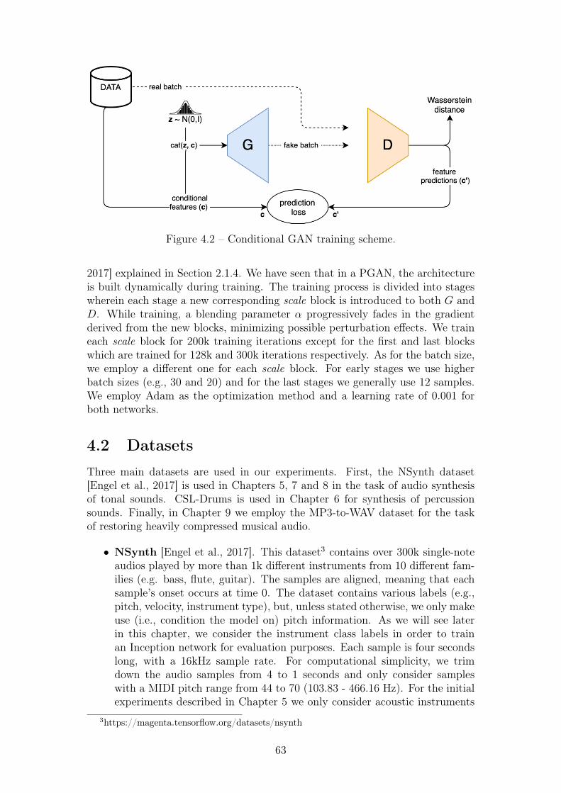
Figure 4.2 – Conditional GAN training scheme.

2017] explained in Section 2.1.4. We have seen that in a PGAN, the architectureis built dynamically during training. The training process is divided into stageswherein each stage a new corresponding scale block is introduced to both G andD. While training, a blending parameter α progressively fades in the gradientderived from the new blocks, minimizing possible perturbation effects. We traineach scale block for 200k training iterations except for the first and last blockswhich are trained for 128k and 300k iterations respectively. As for the batch size,we employ a different one for each scale block. For early stages we use higherbatch sizes (e.g., 30 and 20) and for the last stages we generally use 12 samples.We employ Adam as the optimization method and a learning rate of 0.001 forboth networks.

4.2 DatasetsThree main datasets are used in our experiments. First, the NSynth dataset[Engel et al., 2017] is used in Chapters 5, 7 and 8 in the task of audio synthesisof tonal sounds. CSL-Drums is used in Chapter 6 for synthesis of percussionsounds. Finally, in Chapter 9 we employ the MP3-to-WAV dataset for the taskof restoring heavily compressed musical audio.

• NSynth [Engel et al., 2017]. This dataset3 contains over 300k single-noteaudios played by more than 1k different instruments from 10 different fam-ilies (e.g. bass, flute, guitar). The samples are aligned, meaning that eachsample’s onset occurs at time 0. The dataset contains various labels (e.g.,pitch, velocity, instrument type), but, unless stated otherwise, we only makeuse (i.e., condition the model on) pitch information. As we will see laterin this chapter, we consider the instrument class labels in order to trainan Inception network for evaluation purposes. Each sample is four secondslong, with a 16kHz sample rate. For computational simplicity, we trimdown the audio samples from 4 to 1 seconds and only consider sampleswith a MIDI pitch range from 44 to 70 (103.83 - 466.16 Hz). For the initialexperiments described in Chapter 5 we only consider acoustic instruments

3https://magenta.tensorflow.org/datasets/nsynth

63

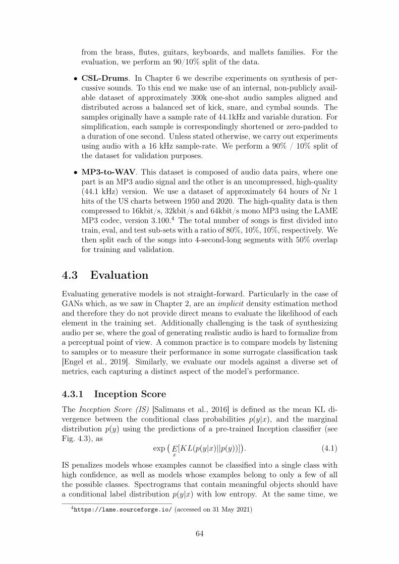
from the brass, flutes, guitars, keyboards, and mallets families. For theevaluation, we perform an 90/10% split of the data.

• CSL-Drums. In Chapter 6 we describe experiments on synthesis of per-cussive sounds. To this end we make use of an internal, non-publicly avail-able dataset of approximately 300k one-shot audio samples aligned anddistributed across a balanced set of kick, snare, and cymbal sounds. Thesamples originally have a sample rate of 44.1kHz and variable duration. Forsimplification, each sample is correspondingly shortened or zero-padded toa duration of one second. Unless stated otherwise, we carry out experimentsusing audio with a 16 kHz sample-rate. We perform a 90% / 10% split ofthe dataset for validation purposes.

• MP3-to-WAV. This dataset is composed of audio data pairs, where onepart is an MP3 audio signal and the other is an uncompressed, high-quality(44.1 kHz) version. We use a dataset of approximately 64 hours of Nr 1hits of the US charts between 1950 and 2020. The high-quality data is thencompressed to 16kbit/s, 32kbit/s and 64kbit/s mono MP3 using the LAMEMP3 codec, version 3.100.4 The total number of songs is first divided intotrain, eval, and test sub-sets with a ratio of 80%, 10%, 10%, respectively. Wethen split each of the songs into 4-second-long segments with 50% overlapfor training and validation.

4.3 EvaluationEvaluating generative models is not straight-forward. Particularly in the case ofGANs which, as we saw in Chapter 2, are an implicit density estimation methodand therefore they do not provide direct means to evaluate the likelihood of eachelement in the training set. Additionally challenging is the task of synthesizingaudio per se, where the goal of generating realistic audio is hard to formalize froma perceptual point of view. A common practice is to compare models by listeningto samples or to measure their performance in some surrogate classification task[Engel et al., 2019]. Similarly, we evaluate our models against a diverse set ofmetrics, each capturing a distinct aspect of the model’s performance.

4.3.1 Inception Score

The Inception Score (IS) [Salimans et al., 2016] is defined as the mean KL di-vergence between the conditional class probabilities p(y|x), and the marginaldistribution p(y) using the predictions of a pre-trained Inception classifier (seeFig. 4.3), as

exp(Ex

[KL(p(y|x)||p(y))]). (4.1)

IS penalizes models whose examples cannot be classified into a single class withhigh confidence, as well as models whose examples belong to only a few of allthe possible classes. Spectrograms that contain meaningful objects should havea conditional label distribution p(y|x) with low entropy. At the same time, we

4https://lame.sourceforge.io/ (accessed on 31 May 2021)

64

Figure 4.3 – Architecture of the Inception Model for image classification as de-scribed by Szegedy et al. [2016]. We adapt this architecture to audio and trainour own inception model on instrument, and/or pitch classification.

expect the model to generate varied sounds, so the marginal∫p(y|x = G(z)) dz

should have high entropy. This metric is found to be useful for the evaluation ofimage models, correlating well with human judgment, although it is not sensibleto over-fitting [Barratt and Sharma, 2018].

Following previous work [Engel et al., 2019], we adapt this metric to audioand train our own Inception network5 to classify the attributes accompanyingthe corresponding dataset, e.g, the instrument and pitch classes in the case ofthose experiments involving the NSynth dataset, or, the instrument class andperceptual features (see Chapter 6) in the case of the CSL-Drums dataset. TheInception model is trained on 1-second long Mel-scaled magnitude STFT spec-trograms with 128 bins. We use a train/validation split of 90% / 10%.

4.3.2 Kernel Inception Distance

The Kernel Inception Distance (KID) [Binkowski et al., 2018] measures the dis-similarity between samples drawn independently from a real pr and generated pgdistributions. It is defined as the squared Maximum Mean Discrepancy (MMD)between representations of the last layer of the same Inception model mentionedin the previous section. A lower MMD means that the generated pg and real prdistributions are close to each other. We employ the unbiased estimator of thesquared MMD [Gretton et al., 2012] between m samples x ∼ pr and n samplesy ∼ pg, for some fixed characteristic kernel function k, defined as

MMD2(X, Y ) =1

m(m− 1)

m∑i 6=j

k(xi, xj)

+1

n(n− 1)

n∑i 6=j

k(yi, yj)

− 2

mn

m∑i=1

n∑j=1

k(xi, yj).

(4.2)

5www.github.com/pytorch/vision/blob/master/torchvision/models/inception.py

65

Here, we use an inverse multi-quadratic kernel (IMQ) k(x, y) = 1/(1 + ||x −y||2/2γ2) with γ2 = 8 [Rustamov, 2019], which has a heavy tail and, hence, it issensitive to outliers.

4.3.3 Fréchet Audio Distance

The Fréchet Audio Distance (FAD) [Kilgour et al., 2018] compares the statisticsof real and generated data computed from an embedding layer of a pre-trainedVGG-like model.6 Viewing the embedding layer as a continuous multivariateGaussian, the mean and co-variance are estimated for real and fake data, and theFAD between these is calculated as

FAD = ||µr − µg||2 + tr(Σr + Σg − 2√

ΣrΣg), (4.3)

where (µr,Σr) and (µg,Σg) are the mean and co-variances of the embedding of realand generated data respectively. Lower FAD means smaller distances betweensynthetic and real data distributions. FAD performs well in terms of robustnessagainst noise, computational efficiency, consistency with human judgments andsensitivity to intra-class mode dropping.

6https://github.com/google-research/google-research/tree/master/frechet_audio_distance

66

67

Chapter 5

Comparing Representations forAudio Synthesis Using GANs

In recent years, deep learning for audio has shifted from using hand-crafted fea-tures requiring prior knowledge, to features learned from raw audio data or mid-level representations such as the Short-Time Fourier Transform (STFT) [Diele-man and Schrauwen, 2014]. Indeed, this has allowed us to build models requiringless prior knowledge, yet at the expense of data, computational power, and train-ing time [Zhu et al., 2016]. For example, deep autoregressive techniques workingdirectly on raw audio [van den Oord et al., 2016a], as well as on Mel-scaled spec-trograms [Vasquez and Lewis, 2019], currently yield state-of-the-art results interms of quality. However, these models can take up to several weeks to train ina conventional GPU, and also, their generation procedure is too slow for typicalproduction environments. On the other hand, GANs [Goodfellow et al., 2014],have achieved comparable audio synthesis quality and faster generation time [En-gel et al., 2019], although they still require long training times and large-scaledatasets when modeling low or mid-level feature representations [Marafioti et al.,2019, Donahue et al., 2019].

It is still subject to debate what the best audio representations are in ma-chine learning in general, and the best choice may also depend on the respectiveapplication and the models employed. In audio synthesis with GANs, differentrepresentations may result in different training and generation times, and mayalso influence the quality of the resulting output. For example, operating onrepresentations that compress the information with respect to perceptual princi-ples, or are structured to better support a specific model architecture, may yieldfaster training and generation times, but may result in worse audio quality. Inthis chapter we compare different audio signal representations, including the rawaudio waveform and a variety of time-frequency representations, for the task ofadversarial audio synthesis with GANs. To this end, we evaluate our models usingthe evaluation metrics described in Sec. 4.3 and report on the respective train-ing, generation, and inversion times. Furthermore, we investigate whether globalattribute conditioning may improve the quality and coherence of the generatedaudio. For that, we perform extensive experimental evaluation when conditioningour models on the pitch information, as well as in a fully unconditional setting.We use the Progressive Growing Wasserstein GAN described in Sec. 4.1.

The content of this chapter is extracted from our paper:

68

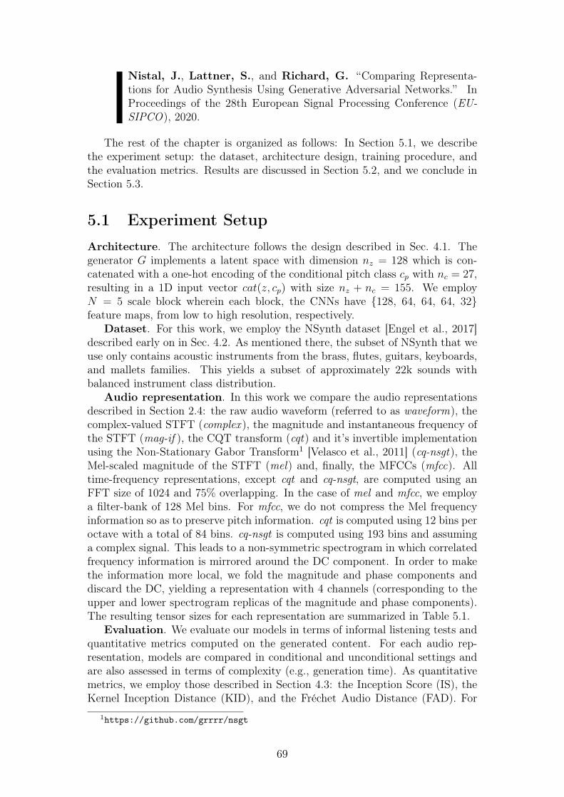
Nistal, J., Lattner, S., and Richard, G. “Comparing Representa-tions for Audio Synthesis Using Generative Adversarial Networks.” InProceedings of the 28th European Signal Processing Conference (EU-SIPCO), 2020.

The rest of the chapter is organized as follows: In Section 5.1, we describethe experiment setup: the dataset, architecture design, training procedure, andthe evaluation metrics. Results are discussed in Section 5.2, and we conclude inSection 5.3.

5.1 Experiment SetupArchitecture. The architecture follows the design described in Sec. 4.1. Thegenerator G implements a latent space with dimension nz = 128 which is con-catenated with a one-hot encoding of the conditional pitch class cp with nc = 27,resulting in a 1D input vector cat(z, cp) with size nz + nc = 155. We employN = 5 scale block wherein each block, the CNNs have {128, 64, 64, 64, 32}feature maps, from low to high resolution, respectively.

Dataset. For this work, we employ the NSynth dataset [Engel et al., 2017]described early on in Sec. 4.2. As mentioned there, the subset of NSynth that weuse only contains acoustic instruments from the brass, flutes, guitars, keyboards,and mallets families. This yields a subset of approximately 22k sounds withbalanced instrument class distribution.

Audio representation. In this work we compare the audio representationsdescribed in Section 2.4: the raw audio waveform (referred to as waveform), thecomplex-valued STFT (complex ), the magnitude and instantaneous frequency ofthe STFT (mag-if ), the CQT transform (cqt) and it’s invertible implementationusing the Non-Stationary Gabor Transform1 [Velasco et al., 2011] (cq-nsgt), theMel-scaled magnitude of the STFT (mel) and, finally, the MFCCs (mfcc). Alltime-frequency representations, except cqt and cq-nsgt, are computed using anFFT size of 1024 and 75% overlapping. In the case of mel and mfcc, we employa filter-bank of 128 Mel bins. For mfcc, we do not compress the Mel frequencyinformation so as to preserve pitch information. cqt is computed using 12 bins peroctave with a total of 84 bins. cq-nsgt is computed using 193 bins and assuminga complex signal. This leads to a non-symmetric spectrogram in which correlatedfrequency information is mirrored around the DC component. In order to makethe information more local, we fold the magnitude and phase components anddiscard the DC, yielding a representation with 4 channels (corresponding to theupper and lower spectrogram replicas of the magnitude and phase components).The resulting tensor sizes for each representation are summarized in Table 5.1.

Evaluation. We evaluate our models in terms of informal listening tests andquantitative metrics computed on the generated content. For each audio rep-resentation, models are compared in conditional and unconditional settings andare also assessed in terms of complexity (e.g., generation time). As quantitativemetrics, we employ those described in Section 4.3: the Inception Score (IS), theKernel Inception Distance (KID), and the Fréchet Audio Distance (FAD). For

1https://github.com/grrrr/nsgt

69

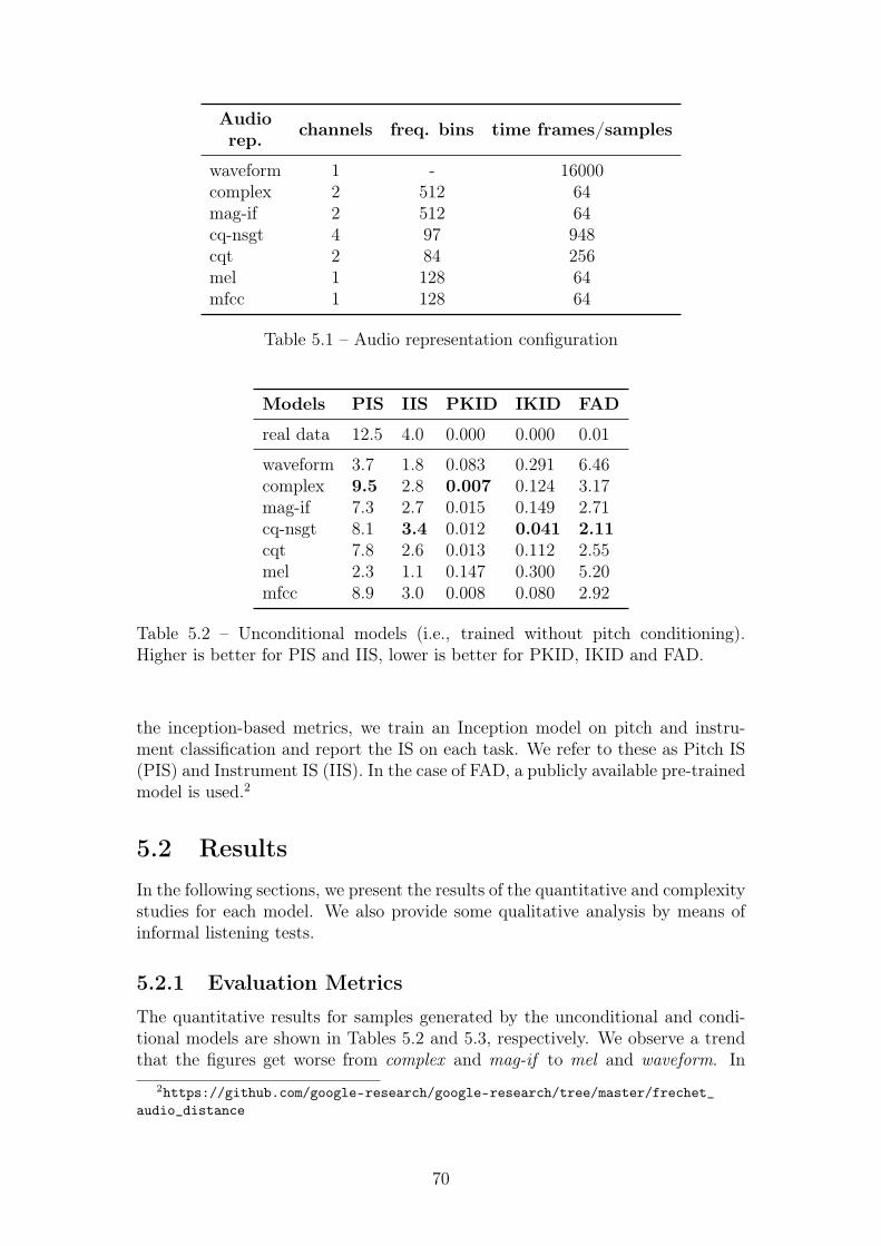
Audiorep. channels freq. bins time frames/samples

waveform 1 - 16000complex 2 512 64mag-if 2 512 64cq-nsgt 4 97 948cqt 2 84 256mel 1 128 64mfcc 1 128 64

Table 5.1 – Audio representation configuration

Models PIS IIS PKID IKID FAD

real data 12.5 4.0 0.000 0.000 0.01

waveform 3.7 1.8 0.083 0.291 6.46complex 9.5 2.8 0.007 0.124 3.17mag-if 7.3 2.7 0.015 0.149 2.71cq-nsgt 8.1 3.4 0.012 0.041 2.11cqt 7.8 2.6 0.013 0.112 2.55mel 2.3 1.1 0.147 0.300 5.20mfcc 8.9 3.0 0.008 0.080 2.92

Table 5.2 – Unconditional models (i.e., trained without pitch conditioning).Higher is better for PIS and IIS, lower is better for PKID, IKID and FAD.

the inception-based metrics, we train an Inception model on pitch and instru-ment classification and report the IS on each task. We refer to these as Pitch IS(PIS) and Instrument IS (IIS). In the case of FAD, a publicly available pre-trainedmodel is used.2

5.2 ResultsIn the following sections, we present the results of the quantitative and complexitystudies for each model. We also provide some qualitative analysis by means ofinformal listening tests.

5.2.1 Evaluation Metrics

The quantitative results for samples generated by the unconditional and condi-tional models are shown in Tables 5.2 and 5.3, respectively. We observe a trendthat the figures get worse from complex and mag-if to mel and waveform. In

2https://github.com/google-research/google-research/tree/master/frechet_audio_distance

70

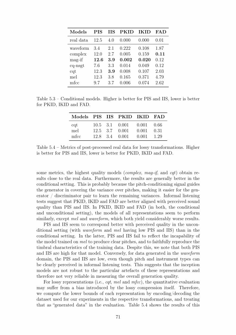
Models PIS IIS PKID IKID FAD

real data 12.5 4.0 0.000 0.000 0.01

waveform 3.4 2.1 0.222 0.108 1.87complex 12.0 2.7 0.005 0.159 0.11mag-if 12.6 3.9 0.002 0.020 0.12cq-nsgt 7.6 3.3 0.014 0.049 0.12cqt 12.3 3.9 0.008 0.107 2.03mel 12.3 3.8 0.165 0.371 4.79mfcc 9.7 3.7 0.006 0.074 2.62

Table 5.3 – Conditional models. Higher is better for PIS and IIS, lower is betterfor PKID, IKID and FAD.

Models PIS IIS PKID IKID FAD

cqt 10.5 3.1 0.001 0.001 0.66mel 12.5 3.7 0.001 0.001 0.31mfcc 12.8 3.4 0.001 0.001 1.29

Table 5.4 – Metrics of post-processed real data for lossy transformations. Higheris better for PIS and IIS, lower is better for PKID, IKID and FAD.

some metrics, the highest quality models (complex, mag-if, and cqt) obtain re-sults close to the real data. Furthermore, the results are generally better in theconditional setting. This is probably because the pitch-conditioning signal guidesthe generator in covering the variance over pitches, making it easier for the gen-erator / discriminator pair to learn the remaining variances. Informal listeningtests suggest that PKID, IKID and FAD are better aligned with perceived soundquality than PIS and IIS. In PKID, IKID and FAD (in both, the conditionaland unconditional setting), the models of all representations seem to performsimilarly, except mel and waveform, which both yield considerably worse results.

PIS and IIS seem to correspond better with perceived quality in the uncon-ditional setting (with waveform and mel having low PIS and IIS) than in theconditional setting. In the latter, PIS and IIS fail to reflect the incapability ofthe model trained on mel to produce clear pitches, and to faithfully reproduce thetimbral characteristics of the training data. Despite this, we note that both PISand IIS are high for that model. Conversely, for data generated in the waveformdomain, the PIS and IIS are low, even though pitch and instrument types canbe clearly perceived in informal listening tests. This suggests that the inceptionmodels are not robust to the particular artefacts of these representations andtherefore not very reliable in measuring the overall generation quality.

For lossy representations (i.e., cqt, mel and mfcc), the quantitative evaluationmay suffer from a bias introduced by the lossy compression itself. Therefore,we compute the lower bounds of each representation by encoding/decoding thedataset used for our experiments in the respective transformations, and treatingthat as “generated data” in the evaluation. Table 5.4 shows the results of this

71

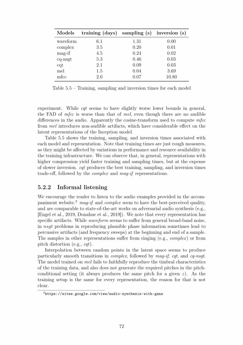
Models training (days) sampling (s) inversion (s)

waveform 6.1 1.31 0.00complex 3.5 0.20 0.01mag-if 4.5 0.24 0.02cq-nsgt 5.3 0.46 0.03cqt 2.1 0.09 0.03mel 1.5 0.04 3.69mfcc 2.0 0.07 10.80

Table 5.5 – Training, sampling and inversion times for each model

experiment. While cqt seems to have slightly worse lower bounds in general,the FAD of mfcc is worse than that of mel, even though there are no audibledifferences in the audio. Apparently the cosine-transform used to compute mfccfrom mel introduces non-audible artifacts, which have considerable effect on thelatent representations of the Inception model.

Table 5.5 shows the training, sampling, and inversion times associated witheach model and representation. Note that training times are just rough measures,as they might be affected by variations in performance and resource availability inthe training infrastructure. We can observe that, in general, representations withhigher compression yield faster training and sampling times, but at the expenseof slower inversion. cqt produces the best training, sampling, and inversion timestrade-off, followed by the complex and mag-if representations.

5.2.2 Informal listening

We encourage the reader to listen to the audio examples provided in the accom-paniment website.3 mag-if and complex seem to have the best-perceived quality,and are comparable to state-of-the-art works on adversarial audio synthesis (e.g.,[Engel et al., 2019, Donahue et al., 2019]). We note that every representation hasspecific artifacts. While waveform seems to suffer from general broad-band noise,in nsgt problems in reproducing plausible phase information sometimes lead topercussive artifacts (and frequency sweeps) at the beginning and end of a sample.The samples in other representations suffer from ringing (e.g., complex ) or frompitch distortion (e.g., cqt).

Interpolation between random points in the latent space seems to produceparticularly smooth transitions in complex, followed by mag-if, cqt, and cq-nsgt.The model trained on mel fails to faithfully reproduce the timbral characteristicsof the training data, and also does not generate the required pitches in the pitch-conditional setting (it always produces the same pitch for a given z). As thetraining setup is the same for every representation, the reason for that is notclear.

3https://sites.google.com/view/audio-synthesis-with-gans

72

5.3 ConclusionThe work described in this chapter compares a variety of audio representations forthe task of adversarial audio synthesis of tonal sounds. We performed quantitativeand qualitative evaluation, and reported on training, generation, and inversiontimes. We found that complex and mag-if yield the best quantitative metrics,which is also aligned with informal listening of the generated samples. Previouswork by Caracalla and Roebel [2020] demonstrated the suitability of the complexspectrogram for sound texture synthesis with CNNs. It is interesting to see thatthis extends to audio generation with GANs. We also found that evaluationmetrics are generally aligned with perceived quality, but in some cases they canbe sensitive to non-audible representation-specific artifacts (e.g., FAD), or yieldfigures which seem over-optimistic when listening to the examples (e.g., PIS andIIS). In the following chapters, we extend this work to explore other types of soundsources such as percussive sounds or music, and experiment with rich conditionalinformation such as perceptual features (see Chapter 6) or semantically intuitiveattributes (see Chapter 7).

73

74

Chapter 6

DrumGAN: Synthesis of DrumSounds with Timbral FeatureConditioning Using GANs

Drum machines are electronic musical instruments that create percussion soundsand allow to arrange them in patterns over time. The sounds produced by someof these machines are often created synthetically using analog or digital signalprocessing. For example, a simple snare drum can be synthesized by generatingnoise and shaping its amplitude envelope [Gordon, 2002b] or, a bass drum, bycombining low-frequency harmonic sine waves with dense mid-frequency compo-nents [Gordon, 2002a]. Generally, drums have been modeled following spectralmodels (see Chapter 3) using subtractive synthesis, or sample-based techniques(e.g., Roland TR-series). The characteristic sound of this synthesis process con-tributed to the cult status of electronic drum machines in the ’80s.

As we have seen throughout Chapters 1 to 3, deep generative neural networksare a viable alternative to traditional signal processing methods for audio synthe-sis. This new paradigm allows us to steer the synthesis process by manipulatinglearned higher-level latent variables or by conditioning the model on preexistingdescriptive information. By doing so, more intuitive controls can be devised foraudio synthesis compared to those systems based on conventional, expert-drivenmechanisms. In addition, as deep learning models can be trained on arbitrarydata, comprehensive control over the generation process can be enabled withoutlimiting the sound characteristic to that of a particular synthesis technique.

We have seen in Chapter 3 that GANs allow to control drum synthesis throughtheir latent input noise [Donahue et al., 2019] and Variational Autoencoders(VAE) can be used to create variations of existing sounds by manipulating theirposition in a learned timbral space [Aouameur et al., 2019]. However, an essentialissue when learning latent spaces in an unsupervised manner is the missing inter-pretability of the learned latent dimensions. This can be a disadvantage in musicapplications, where comprehensible interaction lies at the core of the creativeprocess. Therefore, it is desirable to develop a system which offers expressive andmusically meaningful control over its generated output. A way to achieve this,provided that suitable annotations are available, is to feed higher-level condition-ing information to the model. The user can then manipulate this conditioninginformation in the generation process. Along this line, in previous chapters we

75

studied works on neural audio synthesis that incorporate pitch-conditioning [En-gel et al., 2017, 2019], or categorical semantic tags [Esling et al., 2019], capturingrather abstract sound characteristics. In the case of drum pattern generation,there are approaches that can create full drum tracks conditioned on existingmusical material [Lattner and Grachten, 2019].

In a recent study [Ramires et al., 2020], a U-Net is applied to neural drumsound synthesis, conditioned on continuous perceptual features describing tim-bre (e.g., boominess, brightness, depth). These features are computed using theAudio Commons timbre models.1 Compared to prior work, this continuous fea-ture conditioning (instead of using categorical labels) for audio synthesis providesmore fine-grained control to a musician. However, this U-Net approach learns adeterministic mapping of the conditioning input information to the synthesizedaudio. This limits the model’s capacity to capture the variance in the data, re-sulting in a sound quality that does not seem acceptable in a professional musicproduction scenario.

The work described in this chapter builds upon the same idea of conditionalgeneration using continuous perceptual features, but instead of a U-Net, we em-ploy the Progressive Growing Wasserstein GAN (PGAN) [Karras et al., 2017]described in Chapter 4. Our contribution is two-fold. First, we employ a PGANon the task of conditional drum sound synthesis. Second, we use an auxiliaryregression loss term in the discriminator as a means to control audio generationbased on the conditional features. We are not aware of previous work attemptingcontinuous sparse conditioning of GANs for musical audio generation. We con-duct our experiments on a dataset of a large variety of kick, snare, and cymbalsounds comprising approximately 300k samples (see Sec. 4.2). Also, we investi-gate whether the feature conditioning improves the quality and coherence of thegenerated audio. For that, we perform an extensive experimental evaluation ofour model, both in conditional and unconditional settings. Following the method-ology described in Sec.4.3, we evaluate our models by comparing the InceptionScore (IS), the Fréchet Audio Distance (FAD), and the Kernel Inception Distance(KID). Additionally, we evaluate the perceptual feature conditioning by testingif changing the value of a specific input feature yields the expected change of thecorresponding feature in the generated output. Audio samples of DrumGAN canbe found on the accompaniment website.2

The content of this chapter is extracted from our paper:

Nistal, J., Lattner, S., and Richard, G.. “DrumGAN: Synthesisof Drum Sounds with Perceptual Feature Conditioning using GANs.”In Proceedings of the 28th International Society for Music InformationRetrieval (ISMIR), 2020.

The rest of the chapter is organized as follows: Section 6.1 presents the AudioSet ontology and the pre-trained teacher model; in Section 6.2 we describe theexperiment setup; results are presented in Section 6.3; in Section 6.4 we describethe implementation of DrumGAN as VST plugin and, in Section 6.5, we presentthe AI Drum-Kit; we conclude in Section 6.6.

1https://github.com/AudioCommons/ac-audio-extractor2https://sites.google.com/view/drumgan

76

6.1 Audio-Commons Timbre ModelsIn this work we explore perceptually-driven adversarial audio synthesis of percus-sion sounds. To that end, we condition a GAN on perceptually inspired featuresobtained from the Audio Commons project,3 which offers a publicly availablecollection of perceptual models of features that describe high-level timbral prop-erties of the sound. These features are designed from the study of popular timbreratings given to a collection of sounds obtained from Freesound.4 The models arebuilt by combining existing low-level features found in the literature (e.g., spec-tral centroid, dynamic-range, spectral energy ratios, etc), which correlate withthe target properties enumerated below. All features are defined in the range[0-100] although we normalize them to [0-1]. We employ these features as condi-tioning to the generative model. For more information, we direct the reader tothe project deliverable.3

• brightness: refers to the clarity and amount of high-pitched content in theanalyzed sound. It is computed from the spectral centroid and the spectralenergy ratio.

• hardness: refers to the stiffness or solid nature of the acoustic source thatcould have produced a sound. It is estimated using a linear regression modelon spectral and temporal features extracted from the attack segment of asound event.

• depth: refers to the sensation of perceiving a sound coming from an acous-tic source beneath the surface. A linear regression model estimates depthfrom the spectral centroid of the lower frequencies, the proportion of lowfrequency energy and the low-frequency limit of the audio excerpt.

• roughness: refers to the irregular and uneven sonic texture of a sound. Itis estimated from the interaction of peaks and nearby bins within frequencyspectral frames. When neighboring frequency components have peaks withsimilar amplitude, the sound is said to produce a ‘rough’ sensation.

• boominess: refers to a sound with deep and loud resonant components.5

• warmth: refers to sounds that induce a sensation analogous to that causedby the physical temperature. 5

• sharpness: refers to a sound that might cut if it were to take on physicalform. 5

6.2 Experiment SetupIn this section details are given about the conducted experiments, including thedata used, the model architecture and training details, as well as the metricsemployed for evaluation.

3https://www.audiocommons.org/2018/07/15/audio-commons-audio-extractor.html4https://freesound.org/5Description of the calculation method for this feature is not available to the authors at

current time.

77

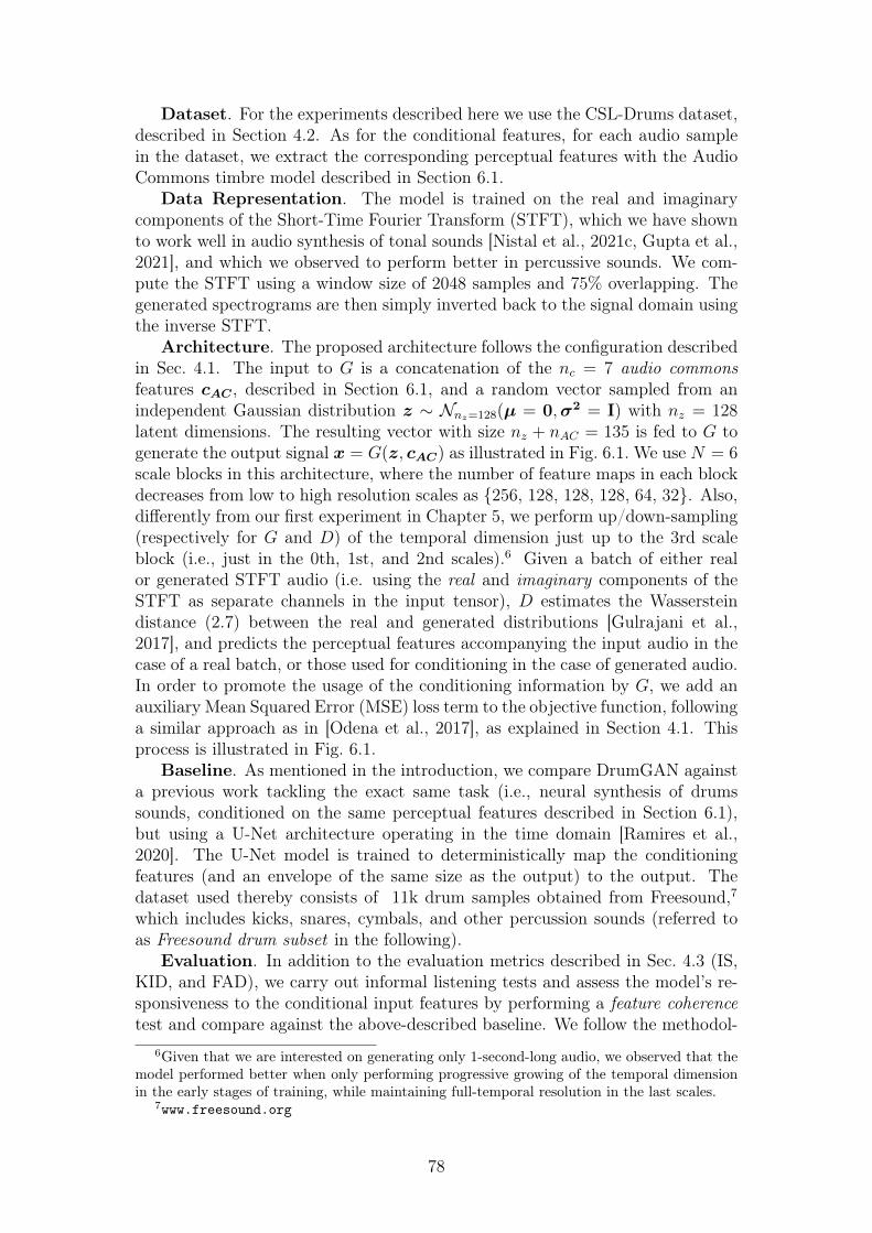
Dataset. For the experiments described here we use the CSL-Drums dataset,described in Section 4.2. As for the conditional features, for each audio samplein the dataset, we extract the corresponding perceptual features with the AudioCommons timbre model described in Section 6.1.

Data Representation. The model is trained on the real and imaginarycomponents of the Short-Time Fourier Transform (STFT), which we have shownto work well in audio synthesis of tonal sounds [Nistal et al., 2021c, Gupta et al.,2021], and which we observed to perform better in percussive sounds. We com-pute the STFT using a window size of 2048 samples and 75% overlapping. Thegenerated spectrograms are then simply inverted back to the signal domain usingthe inverse STFT.

Architecture. The proposed architecture follows the configuration describedin Sec. 4.1. The input to G is a concatenation of the nc = 7 audio commonsfeatures cAC , described in Section 6.1, and a random vector sampled from anindependent Gaussian distribution z ∼ Nnz=128(µ = 0,σ2 = I) with nz = 128latent dimensions. The resulting vector with size nz + nAC = 135 is fed to G togenerate the output signal x = G(z, cAC) as illustrated in Fig. 6.1. We use N = 6scale blocks in this architecture, where the number of feature maps in each blockdecreases from low to high resolution scales as {256, 128, 128, 128, 64, 32}. Also,differently from our first experiment in Chapter 5, we perform up/down-sampling(respectively for G and D) of the temporal dimension just up to the 3rd scaleblock (i.e., just in the 0th, 1st, and 2nd scales).6 Given a batch of either realor generated STFT audio (i.e. using the real and imaginary components of theSTFT as separate channels in the input tensor), D estimates the Wassersteindistance (2.7) between the real and generated distributions [Gulrajani et al.,2017], and predicts the perceptual features accompanying the input audio in thecase of a real batch, or those used for conditioning in the case of generated audio.In order to promote the usage of the conditioning information by G, we add anauxiliary Mean Squared Error (MSE) loss term to the objective function, followinga similar approach as in [Odena et al., 2017], as explained in Section 4.1. Thisprocess is illustrated in Fig. 6.1.

Baseline. As mentioned in the introduction, we compare DrumGAN againsta previous work tackling the exact same task (i.e., neural synthesis of drumssounds, conditioned on the same perceptual features described in Section 6.1),but using a U-Net architecture operating in the time domain [Ramires et al.,2020]. The U-Net model is trained to deterministically map the conditioningfeatures (and an envelope of the same size as the output) to the output. Thedataset used thereby consists of 11k drum samples obtained from Freesound,7which includes kicks, snares, cymbals, and other percussion sounds (referred toas Freesound drum subset in the following).

Evaluation. In addition to the evaluation metrics described in Sec. 4.3 (IS,KID, and FAD), we carry out informal listening tests and assess the model’s re-sponsiveness to the conditional input features by performing a feature coherencetest and compare against the above-described baseline. We follow the methodol-

6Given that we are interested on generating only 1-second-long audio, we observed that themodel performed better when only performing progressive growing of the temporal dimensionin the early stages of training, while maintaining full-temporal resolution in the last scales.

7www.freesound.org

78

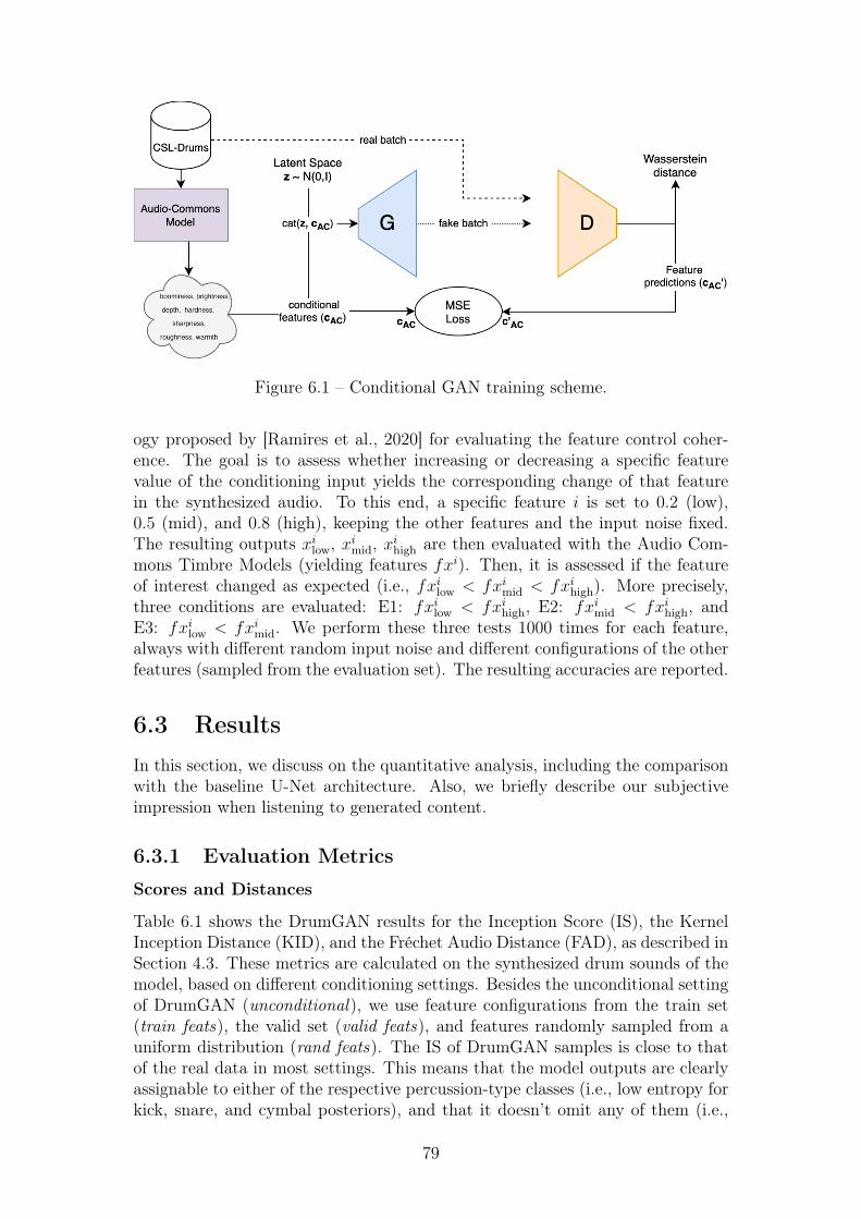
Figure 6.1 – Conditional GAN training scheme.

ogy proposed by [Ramires et al., 2020] for evaluating the feature control coher-ence. The goal is to assess whether increasing or decreasing a specific featurevalue of the conditioning input yields the corresponding change of that featurein the synthesized audio. To this end, a specific feature i is set to 0.2 (low),0.5 (mid), and 0.8 (high), keeping the other features and the input noise fixed.The resulting outputs xilow, ximid, xihigh are then evaluated with the Audio Com-mons Timbre Models (yielding features fxi). Then, it is assessed if the featureof interest changed as expected (i.e., fxilow < fximid < fxihigh). More precisely,three conditions are evaluated: E1: fxilow < fxihigh, E2: fximid < fxihigh, andE3: fxilow < fximid. We perform these three tests 1000 times for each feature,always with different random input noise and different configurations of the otherfeatures (sampled from the evaluation set). The resulting accuracies are reported.

6.3 ResultsIn this section, we discuss on the quantitative analysis, including the comparisonwith the baseline U-Net architecture. Also, we briefly describe our subjectiveimpression when listening to generated content.

6.3.1 Evaluation Metrics

Scores and Distances

Table 6.1 shows the DrumGAN results for the Inception Score (IS), the KernelInception Distance (KID), and the Fréchet Audio Distance (FAD), as described inSection 4.3. These metrics are calculated on the synthesized drum sounds of themodel, based on different conditioning settings. Besides the unconditional settingof DrumGAN (unconditional), we use feature configurations from the train set(train feats), the valid set (valid feats), and features randomly sampled from auniform distribution (rand feats). The IS of DrumGAN samples is close to thatof the real data in most settings. This means that the model outputs are clearlyassignable to either of the respective percussion-type classes (i.e., low entropy forkick, snare, and cymbal posteriors), and that it doesn’t omit any of them (i.e.,

79

high entropy for the marginal over all classes). The IS is slightly reduced forrandom conditioning features, indicating that using uncommon conditioning con-figurations makes the outputs more ambiguous with respect to specific percussiontypes. While FAD is a measure for the perceived quality of the individual sounds(measuring co-variances within data instances), the KID reflects if the generateddata overall follows the distribution of the real data. Therefore, it is interestingto see that rand feats cause outputs which overall do not follow the distributionof the real data (i.e., high KID), but the individual outputs are still plausiblepercussion samples (i.e., low FAD). This quantitative result is in-line with theperceived quality of the generated samples (see Section 6.3.2). In the uncondi-tional setting, both KID and FAD are worse, indicating that feature conditioninghelps the model to both generate data following the true distribution, overall, aswell as in individual samples.

Table 6.2 shows the evaluation results for the U-Net architecture (see Section6.2). As the train / valid split for the Freesound drum subset (on which the U-Net was trained) is not available to the authors, the U-Net model is tested usingthe features of the full Freesound drum subset (real feats), as well as randomfeatures. Also, we do not report the IS for the U-Net architecture, as it wastrained on data without percussion-type labels, making it impossible to train theinception model on such targets. As a baseline, all metrics are also evaluatedon the real data on which the respective models were trained. While evaluationon the real data is straight-forward for the IS (i.e., just using the original datainstead of the generated data to obtain the statistics), both KID and FAD aremeasures usually comparing the statistics between features of real and generateddata. Therefore, for the real data baseline, we split the real data into two equalparts and compare those with each other in order to obtain KID and FAD. Theperformance of the U-Net approach on both, KID and FAD is considerably worsethan that of DrumGAN. While the KID for real feats is still comparable to thatof DrumGAN (indicating a distribution similar to that of the real data), the highFAD indicates that the generated samples are not perceptually similar to thereal samples. When using random feature combinations this trend is accentuatedmoderately in the case of FAD, and particularly in the case of the KID, reachinga maximum of almost 14. This is, however, understandable, as the output ofthe U-Net depends only on the input features in a deterministic way. Therefore,it is expected that the distribution over output samples greatly changes whenperturbating the distribution of the inputs.

Feature Coherence

Table 6.3 shows the accuracy of the three feature coherence tests explained inSection 6.2. Note that, as both models were trained on different data, the figuresof the two models are not directly comparable. However, also reporting the figuresof the U-Net approach should provide some context on the performance of ourproposed model. In addition, as both works use the same feature extractors andclaim that the conditional features are used to shape the same characteristics ofthe output, we consider the figures from the U-Net approach a useful reference.We can see that for about half the features, the U-Net approach reaches close to100% accuracy. Referring to the descriptions on how the features are computed itseems that the U-Net approach reaches particularly high accuracies for features

80

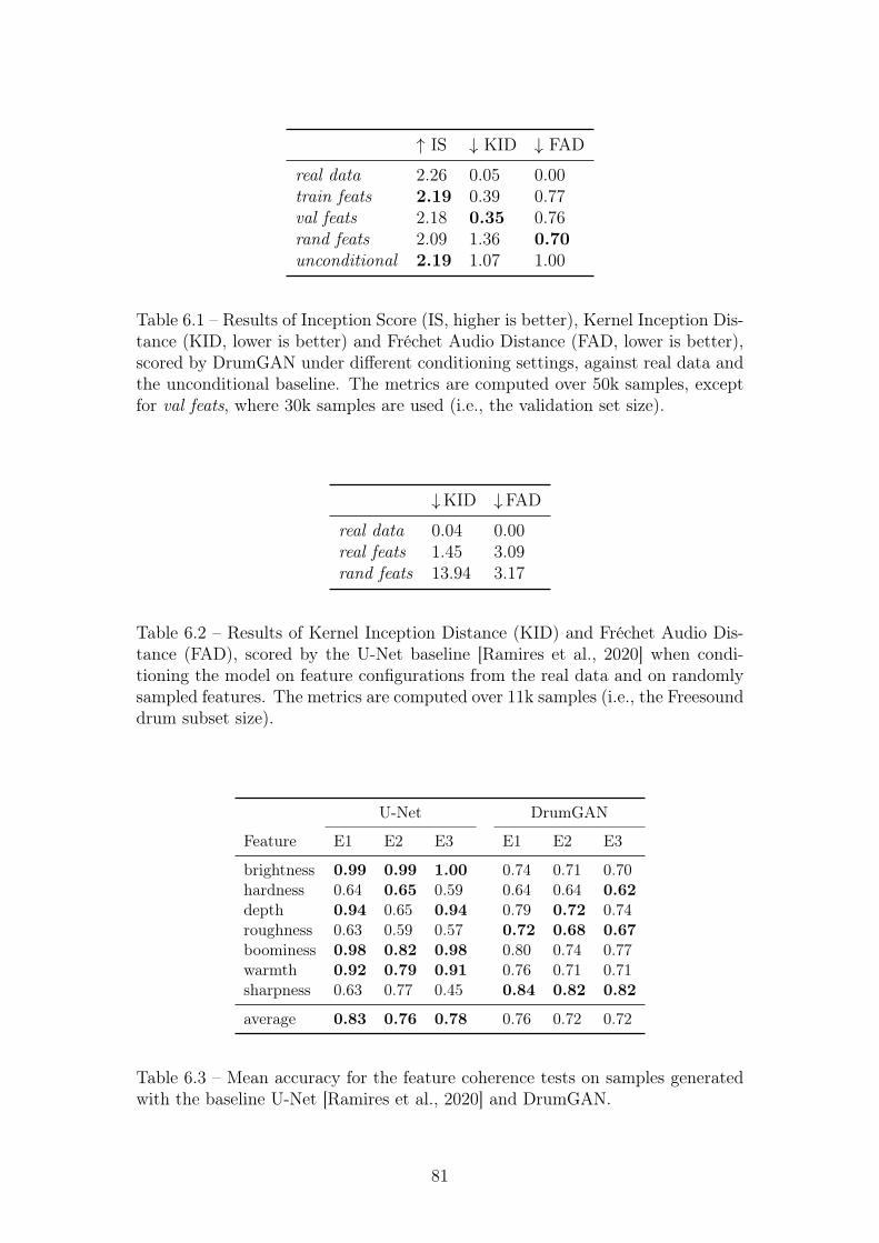
↑ IS ↓ KID ↓ FAD

real data 2.26 0.05 0.00train feats 2.19 0.39 0.77val feats 2.18 0.35 0.76rand feats 2.09 1.36 0.70unconditional 2.19 1.07 1.00

Table 6.1 – Results of Inception Score (IS, higher is better), Kernel Inception Dis-tance (KID, lower is better) and Fréchet Audio Distance (FAD, lower is better),scored by DrumGAN under different conditioning settings, against real data andthe unconditional baseline. The metrics are computed over 50k samples, exceptfor val feats, where 30k samples are used (i.e., the validation set size).

↓KID ↓FAD

real data 0.04 0.00real feats 1.45 3.09rand feats 13.94 3.17

Table 6.2 – Results of Kernel Inception Distance (KID) and Fréchet Audio Dis-tance (FAD), scored by the U-Net baseline [Ramires et al., 2020] when condi-tioning the model on feature configurations from the real data and on randomlysampled features. The metrics are computed over 11k samples (i.e., the Freesounddrum subset size).

U-Net DrumGAN

Feature E1 E2 E3 E1 E2 E3

brightness 0.99 0.99 1.00 0.74 0.71 0.70hardness 0.64 0.65 0.59 0.64 0.64 0.62depth 0.94 0.65 0.94 0.79 0.72 0.74roughness 0.63 0.59 0.57 0.72 0.68 0.67boominess 0.98 0.82 0.98 0.80 0.74 0.77warmth 0.92 0.79 0.91 0.76 0.71 0.71sharpness 0.63 0.77 0.45 0.84 0.82 0.82

average 0.83 0.76 0.78 0.76 0.72 0.72

Table 6.3 – Mean accuracy for the feature coherence tests on samples generatedwith the baseline U-Net [Ramires et al., 2020] and DrumGAN.

81

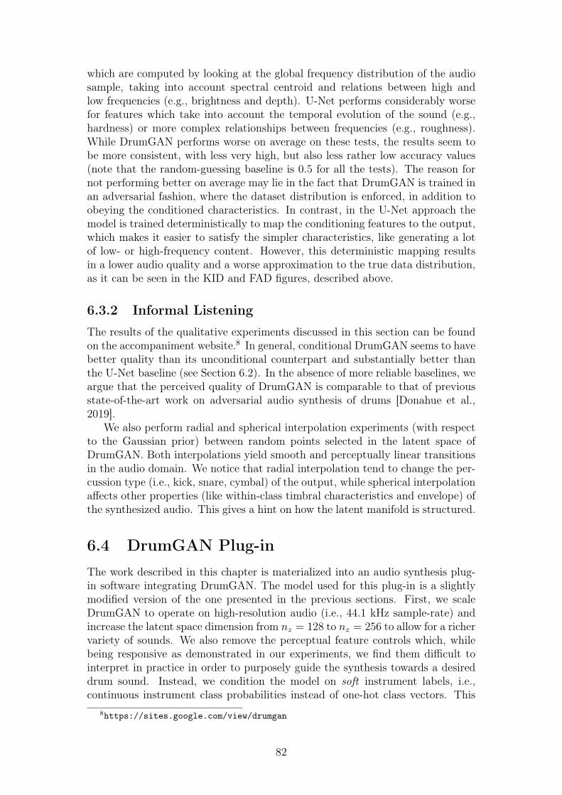
which are computed by looking at the global frequency distribution of the audiosample, taking into account spectral centroid and relations between high andlow frequencies (e.g., brightness and depth). U-Net performs considerably worsefor features which take into account the temporal evolution of the sound (e.g.,hardness) or more complex relationships between frequencies (e.g., roughness).While DrumGAN performs worse on average on these tests, the results seem tobe more consistent, with less very high, but also less rather low accuracy values(note that the random-guessing baseline is 0.5 for all the tests). The reason fornot performing better on average may lie in the fact that DrumGAN is trained inan adversarial fashion, where the dataset distribution is enforced, in addition toobeying the conditioned characteristics. In contrast, in the U-Net approach themodel is trained deterministically to map the conditioning features to the output,which makes it easier to satisfy the simpler characteristics, like generating a lotof low- or high-frequency content. However, this deterministic mapping resultsin a lower audio quality and a worse approximation to the true data distribution,as it can be seen in the KID and FAD figures, described above.

6.3.2 Informal Listening

The results of the qualitative experiments discussed in this section can be foundon the accompaniment website.8 In general, conditional DrumGAN seems to havebetter quality than its unconditional counterpart and substantially better thanthe U-Net baseline (see Section 6.2). In the absence of more reliable baselines, weargue that the perceived quality of DrumGAN is comparable to that of previousstate-of-the-art work on adversarial audio synthesis of drums [Donahue et al.,2019].

We also perform radial and spherical interpolation experiments (with respectto the Gaussian prior) between random points selected in the latent space ofDrumGAN. Both interpolations yield smooth and perceptually linear transitionsin the audio domain. We notice that radial interpolation tend to change the per-cussion type (i.e., kick, snare, cymbal) of the output, while spherical interpolationaffects other properties (like within-class timbral characteristics and envelope) ofthe synthesized audio. This gives a hint on how the latent manifold is structured.

6.4 DrumGAN Plug-inThe work described in this chapter is materialized into an audio synthesis plug-in software integrating DrumGAN. The model used for this plug-in is a slightlymodified version of the one presented in the previous sections. First, we scaleDrumGAN to operate on high-resolution audio (i.e., 44.1 kHz sample-rate) andincrease the latent space dimension from nz = 128 to nz = 256 to allow for a richervariety of sounds. We also remove the perceptual feature controls which, whilebeing responsive as demonstrated in our experiments, we find them difficult tointerpret in practice in order to purposely guide the synthesis towards a desireddrum sound. Instead, we condition the model on soft instrument labels, i.e.,continuous instrument class probabilities instead of one-hot class vectors. This

8https://sites.google.com/view/drumgan

82

way one can continuously and independently control at run-time the specificamount of each instrument class to be synthesized (i.e., some sort of "kickness","snareness" or "cymbalness" control), enabling instrument interpolation. Finally,we also trained an encoder that enables to map any preexisting sound into thelatent space of DrumGAN for its re-synthesis, enabling to generate variations ofit. The interface of this plug-in is illustrated in Fig. 6.2.

Figure 6.2 – DrumGAN’s Graphical User Interface (GUI) developed by CyranAouameur.

The resulting software was showcased at the Sony Technology Exchange Fair2020 (STEF), an internal event for transferring technology across all Sony divi-sions. At STEF, DrumGAN was chosen among 10 projects from more than 300to be demoed in front of some of Sony’s executive officers, including the Vice-President. Also, the visibility in STEF helped foster collaboration around audioGAN research between Sony CSL and other departments such as Sony InteractiveEntertainment (SIE), Sony R&D India, or Sony Music Japan (SMJ).9 Further-more, as part of an ongoing collaboration between Sony CSL and Steinberg,10 apost-doc project is being planned aimed at further extending DrumGAN for itsdeployment and commercialization.

9As a result of the collaboration with SMJ, we created ChainsawGAN, an adaptation ofDrumGAN to chainsaw sound synthesis to be used in the production of a soundtrack for theanime series The Chainsaw Man.

10https://steinberg.net

83

6.5 The A.I. Drum-Kit«The A.I. Drum Kit»11 is a collection of drums generated using DrumGAN andother DL-driven tools built at Sony CSL. It consists of 18 808-like samples, 20kicks, 29 snares, 15 claps, 8 rimshots, 15 hi-hats, 8 open hats, and 12 percs. Thecollection was carefully curated by Sony ATV artist Twenty9 who is a platinumHip-Hop producer collaborating with Sony CSL’s music team. This collectionmelts Twenty9’s know-how experience and lofi trap-like musical style with thecharacteristic sounds of DL-generated drums. The collection was publicly releasedtogether with a teaser (see Fig. 6.3) and can be downloaded for free.12

Figure 6.3 – A frame-shot from the teaser

6.6 ConclusionIn this work, we presented DrumGAN, an adversarial audio synthesizer of drumsounds. DrumGAN’s generation process can be steered using perceptually mo-tivated controls. To this end, we collected the CSL-Drums dataset, described inSection 4.2, and consisting of approximately 300k audio samples containing kicks,snares, and cymbals. We extracted a set of timbral features describing high-levelsemantics of the sound, and used these as conditional input to our model. Weencouraged the generator to use the conditioning information by performing anauxiliary feature regression task in the discriminator and adding the correspond-ing MSE loss term to the objective function. In order to assess whether thefeature conditioning improves the generative process, we trained a model in acompletely unsupervised manner for comparison. We evaluated the models bycomparing various metrics, each reflecting different characteristics of the gener-ation process. Additionally, we compared the coherence of the feature controlagainst previous work. Results showed that DrumGAN generates high-quality

11https://csl.sony.fr/the-a-i-drum-kit-by-twenty9-and-sony-csl/12https://twenty9.beatstars.com/

84

drum samples and provides meaningful control over the audio generation. Theconditioning information was proven to help the network to better approximatethe real distribution of the data. Further, DrumGAN was extended and scaledto operate on high-resolution audio standards (e.g., 44.1kHz sample rate), and itwas implemented in a commercially viable plug-in compatible with any DigitalAudio Workstation (DAW).

85

86

Chapter 7

DarkGAN: Exploiting KnowledgeDistillation for ComprehensibleAudio Synthesis with GANs

In Chapters 2 and 3, we reviewed some of the most outstanding works on audioand image generation using Generative Adversarial Networks (GANs) [Karraset al., 2020, Brock et al., 2019, Park et al., 2019, Engel et al., 2019, Nistal et al.,2020]. An open challenge in GANs is to learn comprehensible features that cap-ture semantically meaningful properties of the data. This has been addressed tosome extent in image generation tasks, where semantic control is achieved us-ing semantic layouts [Park et al., 2019] or high-level attributes learned throughunsupervised methods [Karras et al., 2020]. Other works achieve disentangle-ment of features in the data through regularization terms [Peebles et al., 2020]or by exploring the latent space of the GAN after being trained, in the search forhuman-interpretable factors of variation [Voynov and Babenko, 2020, Shen et al.,2020]. However, the great success of some of these approaches is partly enabledby the availability of large-scale image datasets containing rich semantic annota-tions [Deng et al., 2009, Caesar et al., 2018, Xiao et al., 2017]. Unfortunately, thesituation is different in the musical audio domain, where datasets are scarce andoften limited in size and availability of annotations.

Therefore, the work presented in this chapter studies whether limited annota-tions in audio datasets can be circumvented by taking a Knowledge Distillation(KD) approach (see Section 2.2). To that end, we utilize the soft labels gener-ated by a pre-trained audio-tagging system for conditioning a GAN in an audiogeneration task. More precisely, we train the GAN on a subset of the NSynthdataset [Engel et al., 2017], which contains a wide range of instruments fromacoustic, electronic, and synthetic sources. For that dataset we generate softlabels with a publicly available audio-tagging model [Kong et al., 2020b], pre-trained with attributes of the AudioSet ontology [Gemmeke et al., 2017]. Thisontology contains a structured collection of sound events from many differentsources and descriptions of around 600 attributes obtained from YouTube videos(e.g., "singing bowl", "sonar", "car", "siren", or "bird").

The soft labels produced by such audio tagging system indicate how much ofthe different characteristics are contained in a specific sound (e.g., a synthesizersound may have some similarity with a singing bowl or a sonar pulse). There-

87

fore, it is theoretically possible that attributes that do not explicitly exist in thetraining data (e.g., "sonar", "singing bowl"), can still be somehow sparsely en-coded across many examples. We hope that the generative model can distill suchcharacteristics (e.g., the "essence" of a singing bowl sound) by looking at the softlabels to then be able to emphasize them at generation. The slight similaritiesto specific categories in data that can be distilled using soft labels were coined"Dark Knowledge" [Hinton et al., 2015]. Therefore, we call the proposed modelDarkGAN.

The work contained in this chapter introduces a generic audio cross-task KDframework for transferring semantically meaningful features into a neural audiosynthesizer. We implement this framework in DarkGAN, an adversarial audiosynthesizer for comprehensible and controllable audio synthesis. We perform anexperimental evaluation on the quality of the generated material and the seman-tic consistency of the learned attribute controls. Numerous audio examples areprovided in the accompanying web page,1 and the code is released for repro-ducibility.2

The content of this chapter is extracted from our paper:

Nistal, J., Lattner, S., and Richard, G.. “DarkGAN: Exploit-ing Knoweldge Distillation for Comprehensible Audio Synthesis WithGANs.” In Proceedings of the 29th International Society for Music In-formation Retrieval (ISMIR), 2021.

In what follows, we first mention relevant state-of-the-art works in knowledgedistillation, giving special attention to those works focused on audio (see Section7.1). Next, in Section 7.2 we describe the AudioSet ontology and the pre-trainedaudio tagging system that we use as teacher model. We then present the exper-imental framework of DarkGAN (see Section 7.3). In Section 7.4 we provide adiscussion of the results, and conclude in Section 7.5.

7.1 Previous WorkThe Knowledge Distillation (KD) framework was briefly described in Section 2.2.As mentioned there, KD has been generally used as a model compression tech-nique, although a few works employ it for different purposes [Papernot et al.,2017, Anil et al., 2018, Yuan and Peng, 2020]. For example, some works exploreKD as a means to secure privacy of medical history training data, by releasing tothe public models that are not explicitly trained on the sensible dataset, but onaggregated predictions of teacher ensembles [Papernot et al., 2017]. Other worksemploy KD on-the-fly as a distributed training framework to train very largemodels, and scale beyond the limits of distributed stochastic gradient descent[Anil et al., 2018]. An interesting line of research that is closely related to oursproposes cross-task knowledge distillation from image captioning and classifica-tion systems into an image synthesis generative neural-network [Yuan and Peng,2018, 2020]. In audio, KD was extensively used on Automatic Speech Recogni-tion (ASR) tasks in order to exploit large unlabelled datasets [Li et al., 2014],

1https://an-1673.github.io/DarkGAN.io/2https://github.com/SonyCSLParis/DarkGAN

88

distill the knowledge from deep Recurrent Neural Networks (RNN) [Chan et al.,2015] or, inversely, to improve the performance of deep RNN models by distillingknowledge from simple models as a regularization technique [Tang et al., 2016].Works related to ours use KD as a means to adapt a model to a different audiodomain task [Asami et al., 2017] or even data modality (by distilling knowledgefrom a video classifier) [Aytar et al., 2016], where labeled datasets are scarce,and large models would easily overfit. Some works employ KD to fuse knowl-edge from different audio representations into a single compact model [Gao et al.,2020]. Finally, some works employed probability density distillation to reduce thecomputational complexity of WaveNet and allow parallel generation using stan-dard feed-forward neural-networks [van den Oord et al., 2018a]. Here we employknowledge distillation as a means to learn semantically meaningful controls in anadversarial audio synthesizer. To the best of our knowledge, this is the first timethat such a task has been attempted in audio generation with GANs.

7.2 The AudioSet OntologyAudioSet [Gemmeke et al., 2017] is a large-scale dataset containing audio dataand an ontology of sound events that seeks to describe real-world sounds. Itwas created to set a benchmark in the development of automatic audio eventrecognition systems, similar to those in computer-vision, such as ImageNet [Denget al., 2009]. The dataset consists of a structured vocabulary of 632 audio eventclasses and a collection of approximately 2M human-labeled 10-second soundclips drawn from YouTube videos. The ontology is specified as a hierarchy ofcategories with a maximum depth of 6 levels, covering a wide range of human andanimal sounds, musical genres and instruments, and environmental sounds. Weencourage the reader to visit the corresponding website for a complete descriptionof the ontology.3

In this work, we do not employ all of the AudioSet attributes, as many of themrefer to properties that are too vague for musical sounds or describe broader time-scale aspects of the sound (e.g., music, chatter, sound effect). Instead, we rankthe attributes based on the geometric mean of their 90th percentile (calculatedon the predicted class probabilities for each attribute across the dataset), andthe teacher’s reported accuracy as

√pi90th × acci. Then, we take the first 128

attributes according to this ranking.

7.2.1 Pre-trained AudioSet Classifier

In this work, we distill the knowledge from a pre-trained audio-tagging neuralnetwork (PANN) trained on raw audio recordings from the AudioSet collection[Kong et al., 2020b]. PANNs were originally proposed for transferring knowledgeto other discriminative tasks. However, we use them to transfer the knowledgeto a generative model and enable steering the generation process through a com-prehensible vocabulary of attributes.

We employ the CNN-14 model from the PANNs [Kong et al., 2020b]. CNN-14is built upon a stack of 6 convolution-based blocks containing 2 CNN layers with a

3research.google.com/audioset/ontology/

89

kernel size of 3x3. Batch Normalization is applied after every convolutional layer,and a ReLU non-linearity is used as activation function. After each convolutionalblock, they apply an average-pooling layer of size 2x2 for down-sampling. Globalpooling is applied after the last convolutional layer to summarize the feature mapsinto a fixed-length vector. An extra fully-connected layer is added to extractembedding features before the output Sigmoid activation function. For moredetails on the architecture, please refer to Kong et al. [2020b].

7.3 Experiment SetupIn this section, details are given about the conducted experiments. We describethe AudioSet ontology, provide details about the teacher and student architec-tures, the metrics employed for evaluation, and the baselines used for comparison.

Dataset. For this work, we employ the NSynth dataset [Engel et al., 2017],described early on in Section 4.2. We employ all of the instrument classes (notonly from the acoustic family) yielding to a subset of approximately 90k soundswith balanced instrument class distribution.

Audio representation. Following our previous work comparing represen-tations for audio synthesis [Nistal et al., 2021c] we employ the Magnitude andInstantaneous Frequency of the STFT (mag-if ) as it was shown to work well asa representation for tonal sounds. We use an FFT size of 2048 bins, an overlapof 75%, and a sample-rate of 16kHz.

Architecture. DarkGAN’s architecture, illustrated in Fig. 4.1, follows thearchitecture of DrumGAN [Nistal et al., 2020] (see Chapter 6). The input to G isa concatenation of nAS = 128 teacher-labeled AudioSet attributes cAS ∈ [0, 1]128

(see Sec. 7.2), a one-hot vector cp ∈ {0, 1}26 containing np = 26 pitch classes, anda random vector z ∼ N32(0, 1) with nz = 32 components. The resulting vector isplaced as a column in the middle of a 4D tensor with nC = nz + np + nAS = 186convolutional maps. Then, it is fed through a stack of convolutional and box up-sampling blocks to generate the output signal x = G(z, cp, cAS). We use N = 6scale blocks, wherein each block the number of feature maps decreases from lowto high resolution as {256, 128, 128, 128, 128, 64}. The discriminator D mirrorsG’s configuration and estimates the Wasserstein distance Wd between the realand generated distributions [Gulrajani et al., 2017], and predicts the AudioSetfeatures accompanying the input audio in the case of a real batch, or those used forconditioning in the case of generated audio (see Fig. 7.1). In order to promote theusage of the conditioning information by G, we add to the objective function anauxiliary binary cross-entropy loss term for the distillation task and a categoricalcross-entropy for the pitch classification task [Odena et al., 2017].

Evaluation. This work aims to learn semantically meaningful controls withDarkGAN by distilling knowledge from an audio-tagging system trained on at-tributes from the AudioSet ontology. Therefore, in addition to the evaluationmetrics presented in Sec 4.3, we evaluate if changing an input attribute is reflectedin the corresponding output of DarkGAN. To that end, we examine the changein the prediction of the teacher model (w.r.t. the output of DarkGAN) whenchanging a particular DarkGAN input attribute. A second property to assess iswhether the dark knowledge helps DarkGAN learn well-formed representations ofspecific attributes and generalize to out-of-distribution input combinations. We

90

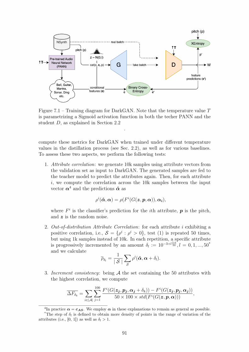
Figure 7.1 – Training diagram for DarkGAN. Note that the temperature value Tis parametrizing a Sigmoid activation function in both the techer PANN and thestudent D, as explained in Section 2.2

.

compute these metrics for DarkGAN when trained under different temperaturevalues in the distillation process (see Sec. 2.2), as well as for various baselines.To assess these two aspects, we perform the following tests:

1. Attribute correlation: we generate 10k samples using attribute vectors fromthe validation set as input to DarkGAN. The generated samples are fed tothe teacher model to predict the attributes again. Then, for each attributei, we compute the correlation across the 10k samples between the inputvector α4 and the predictions α as

ρi(α,α) = ρ(F i(G(z,p,α)),αi),

where F i is the classifier’s prediction for the ith attribute, p is the pitch,and z is the random noise.

2. Out-of-distribution Attribute Correlation: for each attribute i exhibiting apositive correlation, i.e., S = {ρi : ρi > 0}, test (1) is repeated 50 times,but using 1k samples instead of 10k. In each repetition, a specific attributeis progressively incremented by an amount δl := 10−3+l

3.650 , l = 0, 1, ..., 50*

and we calculateρδl =

1

| S |∑S

ρi(α,α+ δl).

3. Increment consistency : being A the set containing the 50 attributes withthe highest correlation, we compute

∆Fδk =∑i∈|A|

100∑j=1

F i(G(zj ,pj ,αj + δk))− F i(G(zj ,pj ,αj))

50× 100× std(F i(G(z,p,α))),

4In practice α = cAS . We employ α in these explanations to remain as general as possible.*The step of δl is defined to obtain more density of points in the range of variation of the

attributes (i.e., [0, 1]) as well as δl > 1.

91

where αj is the jth original feature vector from a set of 100 samples ran-domly picked from the validation set, and δk := k

5, k = 0, 1, ..., 25. Intu-

itively, it is defined as the average difference of the predicted attributesof the generated audios (i.e., the difference before and after the attributeincrement) as a function of the increment δk. We express the result interms of standard deviations of the non-incremented generated examples asstd(G(z,p,α)).

Baselines. We compare the evaluation metrics described above with realdata to obtain a baseline for each metric. Also, GANSynth [Engel et al., 2019],the state-of-the-art on audio synthesis with GANs, is used for comparison.6 AsGANSynth generates 4-second long sounds, the waveform is trimmed down to 1second for comparison with our models. Additionally, we examine the effect thatKD has on these metrics by comparing against a model analogous to DarkGAN,but without using the AudioSet feature conditioning (baseline). Experiment re-sults for DarkGAN are shown for different temperature values T ∈ {1, 1.5, 2, 3, 5}(2.9) as part of the KD process (see Sec. 2.2.1), and we report separate resultsfor conditional attributes obtained from the training (tr) and validation (val) set.

7.4 ResultsIn this section, we present the results from the evaluation procedure described inSec. 7.3. We validate the quantitative results based on an informal assessment ofthe generated content.

7.4.1 Evaluation Metrics

Scores and Distances

Table 7.1 presents the metrics scored by DarkGANT , where T ∈ {1, 1.5, 2, 3, 5}is the temperature value, and the baseline models, as described in Sec. 7.3. Notethat we condition DarkGAN on attribute vectors randomly sampled from the val-idation set. Overall, DarkGANT∈{1.5,2} obtains better results than the baselinesand is close to real data in most metrics. All models score higher PIS than realdata, with GANSynth in the first place, suggesting that the generated exampleshave a clear pitch and that the distribution of pitch classes follows that of thetraining data. This is not surprising, as all the models have explicit pitch condi-tioning. In contrast, we do not provide conditioning attributes for the instrumentclass. Therefore, we observe a slight drop in IIS for all models compared to realdata. DarkGANT∈{1.5,2} achieves the highest IIS, suggesting that the model cap-tured the timbre diversity of the dataset and, also, that the generated soundscan be reliably classified into one of all possible instruments. In terms of KID,DarkGANT∈{1.5,2} and baseline are on a par with real data. A KID equal toreal data indicates that the Inception embeddings are similarly distributed forreal and generated data. As our Inception classifier is trained on pitch and in-strument classification and predicting AudioSet features, similarities in such anembedding space indicate common timbral and tonal characteristics between the

6https://github.com/magenta/magenta/tree/master/magenta/models/gansynth

92

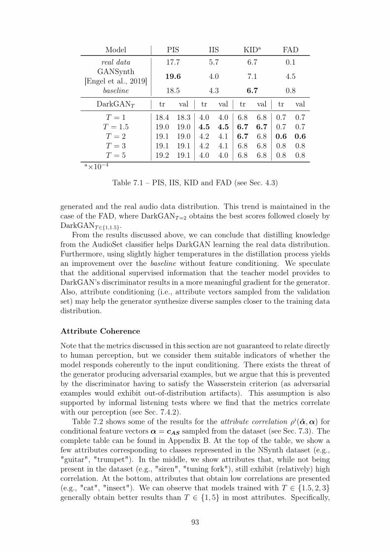
Model PIS IIS KIDa FADreal data 17.7 5.7 6.7 0.1GANSynth

[Engel et al., 2019] 19.6 4.0 7.1 4.5

baseline 18.5 4.3 6.7 0.8

DarkGANT tr val tr val tr val tr val

T = 1 18.4 18.3 4.0 4.0 6.8 6.8 0.7 0.7T = 1.5 19.0 19.0 4.5 4.5 6.7 6.7 0.7 0.7T = 2 19.1 19.0 4.2 4.1 6.7 6.8 0.6 0.6T = 3 19.1 19.1 4.2 4.1 6.8 6.8 0.8 0.8T = 5 19.2 19.1 4.0 4.0 6.8 6.8 0.8 0.8

a×10−4

Table 7.1 – PIS, IIS, KID and FAD (see Sec. 4.3)

generated and the real audio data distribution. This trend is maintained in thecase of the FAD, where DarkGANT=2 obtains the best scores followed closely byDarkGANT∈{1,1.5}.

From the results discussed above, we can conclude that distilling knowledgefrom the AudioSet classifier helps DarkGAN learning the real data distribution.Furthermore, using slightly higher temperatures in the distillation process yieldsan improvement over the baseline without feature conditioning. We speculatethat the additional supervised information that the teacher model provides toDarkGAN’s discriminator results in a more meaningful gradient for the generator.Also, attribute conditioning (i.e., attribute vectors sampled from the validationset) may help the generator synthesize diverse samples closer to the training datadistribution.

Attribute Coherence

Note that the metrics discussed in this section are not guaranteed to relate directlyto human perception, but we consider them suitable indicators of whether themodel responds coherently to the input conditioning. There exists the threat ofthe generator producing adversarial examples, but we argue that this is preventedby the discriminator having to satisfy the Wasserstein criterion (as adversarialexamples would exhibit out-of-distribution artifacts). This assumption is alsosupported by informal listening tests where we find that the metrics correlatewith our perception (see Sec. 7.4.2).

Table 7.2 shows some of the results for the attribute correlation ρi(α,α) forconditional feature vectors α = cAS sampled from the dataset (see Sec. 7.3). Thecomplete table can be found in Appendix B. At the top of the table, we show afew attributes corresponding to classes represented in the NSynth dataset (e.g.,"guitar", "trumpet"). In the middle, we show attributes that, while not beingpresent in the dataset (e.g., "siren", "tuning fork"), still exhibit (relatively) highcorrelation. At the bottom, attributes that obtain low correlations are presented(e.g., "cat", "insect"). We can observe that models trained with T ∈ {1.5, 2, 3}generally obtain better results than T ∈ {1, 5} in most attributes. Specifically,

93

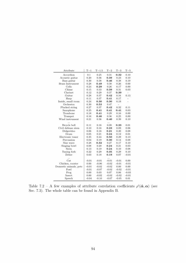
Attribute T=1 T=1.5 T=2 T=3 T=5

Accordion 0.1 0.25 0.31 0.32 0.10Acoustic guitar 0.20 0.36 0.39 0.23 0.10Bass guitar 0.30 0.38 0.46 0.38 0.19

Brass Instrument 0.28 0.49 0.38 0.26 0.00Cello 0.24 0.29 0.26 0.17 0.00Chime 0.15 0.33 0.39 0.31 0.03Clarinet 0.12 0.29 0.37 0.39 -Guitar 0.28 0.37 0.42 0.34 0.13Harp 0.11 0.37 0.41 0.17 -

Inside, small room 0.24 0.30 0.30 0.19 -Orchestra 0.30 0.53 0.47 -

Plucked string 0.27 0.37 0.42 0.32 0.11Saxophone 0.25 0.41 0.41 0.41 0.03Trombone 0.18 0.41 0.29 0.16 0.00Trumpet 0.16 0.46 0.36 0.25 0.00

Wind instrument 0.21 0.36 0.40 0.39 0.10... ...

Bicycle bell 0.11 0.16 0.08 0.23 0.01Civil defense siren 0.10 0.16 0.23 0.09 0.06

Didgeridoo 0.06 0.16 0.21 0.20 0.08Drum 0.05 0.21 0.24 0.12 0.01

Electronic tuner 0.35 0.44 0.50 0.29 0.13Percussion 0.04 0.19 0.30 0.14 0.08Sine wave 0.28 0.32 0.27 0.17 0.10

Singing bowl 0.08 0.20 0.24 0.21 0.03Siren 0.13 0.19 0.24 0.10 0.08

Tuning fork 0.22 0.29 0.35 0.29 0.10Zither 0.03 0.18 0.19 0.07 -0.01... ...Cat -0.01 -0.01 -0.01 -0.01 0.00

Chicken, rooster 0.00 -0.06 -0.02 -0.01 -0.01Domestic animals, pets -0.01 -0.02 -0.02 0.00 0.00

Fowl -0.01 -0.07 -0.02 -0.02 -0.01Frog 0.00 0.03 0.07 0.06 -0.03Insect 0.00 -0.02 -0.02 -0.02 -0.01Speech -0.04 -0.10 -0.07 -0.05 0.01

Table 7.2 – A few examples of attribute correlation coefficients ρi(α,α) (seeSec. 7.3). The whole table can be found in Appendix B.

94

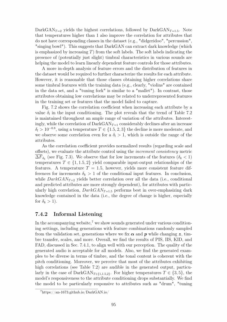
DarkGANT=2 yields the highest correlations, followed by DarkGANT=1.5. Notethat temperatures higher than 1 also improve the correlation for attributes thatdo not have corresponding classes in the dataset (e.g., "didgeridoo", "percussion","singing bowl"). This suggests that DarkGAN can extract dark knowledge (whichis emphasized by increasing T ) from the soft labels. The soft labels indicating thepresence of (potentially just slight) timbral characteristics in various sounds arehelping the model to learn linearly dependent feature controls for those attributes.

A more in-depth analysis of feature errors and the distribution of features inthe dataset would be required to further characterize the results for each attribute.However, it is reasonable that those classes obtaining higher correlations sharesome timbral features with the training data (e.g., clearly, "violins" are containedin the data set, and a "tuning fork" is similar to a "mallet"). In contrast, thoseattributes obtaining low correlations may be related to underrepresented featuresin the training set or features that the model failed to capture.

Fig. 7.2 shows the correlation coefficient when increasing each attribute by avalue δl in the input conditioning. The plot reveals that the trend of Table 7.2is maintained throughout an ample range of variation of the attributes. Interest-ingly, while the correlation of DarkGANT=1 considerably declines after an increaseδl > 10−0.8, using a temperature T ∈ {1.5, 2, 3} the decline is more moderate, andwe observe some correlation even for a δl > 1, which is outside the range of theattributes.

As the correlation coefficient provides normalized results (regarding scale andoffsets), we evaluate the attribute control using the increment consistency metric∆F δk (see Fig. 7.3). We observe that for low increments of the features (δk < 1)temperatures T ∈ {1, 1.5, 2} yield comparable input-output relationships of thefeatures. A temperature T = 1.5, however, yields more consistent feature dif-ferences for increments δk > 1 of the conditional input features. In conclusion,while DarkGANT=2 yields better correlation over all the data (i.e., conditionaland predicted attributes are more strongly dependent), for attributes with partic-ularly high correlation, DarkGANT=1.5 performs best in over-emphasizing darkknowledge contained in the data (i.e., the degree of change is higher, especiallyfor δk > 1).

7.4.2 Informal Listening

In the accompanying website,7 we show sounds generated under various condition-ing settings, including generations with feature combinations randomly sampledfrom the validation set, generations where we fix α and p while changing z, tim-bre transfer, scales, and more. Overall, we find the results of PIS, IIS, KID, andFAD, discussed in Sec. 7.4.1, to align well with our perception. The quality of thegenerated audio is acceptable for all models. Also, we find the generated exam-ples to be diverse in terms of timbre, and the tonal content is coherent with thepitch conditioning. Moreover, we perceive that most of the attributes exhibitinghigh correlations (see Table 7.2) are audible in the generated output, particu-larly in the case of DarkGANT∈{1,1.5,2}. For higher temperatures T ∈ {3, 5}, themodel’s responsiveness to the attribute conditioning drops substantially. We findthe model to be particularly responsive to attributes such as "drum", "tuning

7https://an-1673.github.io/DarkGAN.io/

95

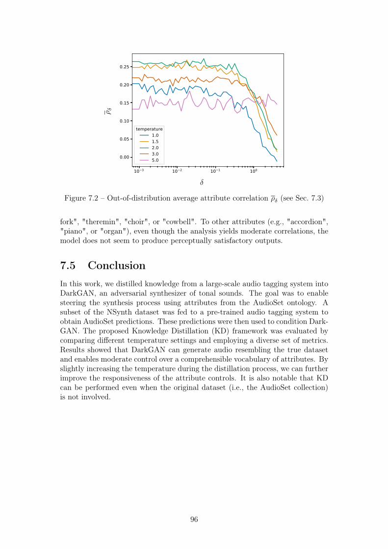
10 3 10 2 10 1 100

0.00

0.05

0.10

0.15

0.20

0.25

F t(G

(z,p

,+

))F t

(G(z

,p,

))st

d

temperature1.01.52.03.05.0

δ

ρδ

Figure 7.2 – Out-of-distribution average attribute correlation ρδ (see Sec. 7.3)

fork", "theremin", "choir", or "cowbell". To other attributes (e.g., "accordion","piano", or "organ"), even though the analysis yields moderate correlations, themodel does not seem to produce perceptually satisfactory outputs.

7.5 ConclusionIn this work, we distilled knowledge from a large-scale audio tagging system intoDarkGAN, an adversarial synthesizer of tonal sounds. The goal was to enablesteering the synthesis process using attributes from the AudioSet ontology. Asubset of the NSynth dataset was fed to a pre-trained audio tagging system toobtain AudioSet predictions. These predictions were then used to condition Dark-GAN. The proposed Knowledge Distillation (KD) framework was evaluated bycomparing different temperature settings and employing a diverse set of metrics.Results showed that DarkGAN can generate audio resembling the true datasetand enables moderate control over a comprehensible vocabulary of attributes. Byslightly increasing the temperature during the distillation process, we can furtherimprove the responsiveness of the attribute controls. It is also notable that KDcan be performed even when the original dataset (i.e., the AudioSet collection)is not involved.

96

0 1 2 3 4 5

0.0

0.5

1.0

1.5

2.0

F t(G

(z,p

,+

))F t

(G(z

,p,

))st

d

temperature1.01.52.03.05.0

δk

∆Fδ k

Figure 7.3 – Increment consistency ∆F δk (see Sec.7.3)

97

98

Chapter 8

VQCPC-GAN: Variable-LengthAdversarial Audio Synthesis UsingVector-Quantized ContrastivePredictive Coding

In recent years, Generative Adversarial Networks (GANs) [Goodfellow et al.,2014] have shown outstanding results in image and audio synthesis tasks [Karraset al., 2017, 2020, Engel et al., 2019, Nistal et al., 2020, Binkowski et al., 2020].As most (initial) studies on GANs focused on generating images, the resultingarchitectures are now often adopted for the musical audio domain, using fixed-sizetwo-dimensional spectrogram representations as the “image data”. However, whileit is a natural choice to use data of fixed dimensionality in the visual domain,fixing the length of musical audio content in generation tasks poses a significantlimitation. As a result, GANs are currently mainly used to generate short audiocontent in the musical audio domain, like single notes of a tonal instrument orsingle percussion samples [Engel et al., 2019, Nistal et al., 2020].

We have seen in Chapter 3 that when dealing with variable-length sequencegeneration, commonly utilized models are Transformer architectures [Hadjeresand Crestel, 2020], causal convolutional architectures (causal CNNs) [van denOord et al., 2016a], and recurrent neural networks (RNNs) [Fan et al., 2014].However, those models suffer various problems like high computational cost (au-toregressive), missing look-back capabilities (recurrent), and, typically, they can-not be parallelized at test time. In contrast, GANs are relatively efficient ingenerating high-dimensional data, as the conditioning on a single noise vectordetermines the values of all output dimensions at once. Therefore, it seems rea-sonable to also adopt the GAN paradigm for generating variable-length musicalaudio content. It has been shown in text-to-speech translation [Binkowski et al.,2020] that GANs can be successful in generating coherent variable-length audiowhen conditioned on meaningful sequences of symbols (i.e., linguistic and pitchfeatures), while the input noise z accounts for the remaining variability.

We adopt a similar strategy by first learning sequences of symbolic audiodescriptors, serving as conditional inputs to a GAN architecture. These descrip-tors are discrete tokens learned through self-supervised training, using Vector-Quantized Contrastive Predictive Coding (VQCPC) [Hadjeres and Crestel, 2020]

99

as explained in Section 2.3. In VQCPC, discrete representations are learnedthrough contrastive learning, by confronting positive and negative examples. Incontrast to reconstruction-based VQ-VAEs, introduced by van den Oord et al.[2017], VQCPC allows to control to some extent which aspects of the (sequential)data are captured in the tokens, by carefully designing a negative sampling strat-egy, thus defining the so-called “pretext” task. In this work, the tokens are trainedto represent time-varying features (i.e., something close to the envelope) of single,pitched audios of different instruments. The proposed model is conditioned onsuch envelope feature sequences, on the noise vector zzz (static, representing the“instrument”), and on pitch information (static). This approach of sequence gen-eration with GANs using discrete tokens is promising for future, more elaborateapplications. While in this work, we are simply up-sampling token sequences togenerate longer sounds, one could also generate plausible token sequences. Sucha system could then be used to hold sounds for an arbitrary time in real-timeperformance with a MIDI input device. Also, token sequences could be gener-ated conditioned on MIDI information, to represent the dynamics of a targetinstrument. The resulting system could then be used for naturalistic renderingof MIDI files. Furthermore, training tokens to also represent pitch informationwould result in a more general variable-length audio generation framework. Tothe best of our knowledge, this is the first work implementing a variable-lengthGAN for musical audio synthesis.

The content of this chapter is extracted from our paper:

Nistal, J., Auoameur, C., Lattner, S., and Richard, G. “VQCPC-GAN: Variable-Length Adversarial Audio Synthesis using Vector-Quantized Contrastive Predictive Coding.” In Workshop on Applicationsof Signal Processing for Audio and Acoustics (WASPAA), 2021.

The rest of this chapter is organized as follows. First, in Section 8.1, we sum-marize previous works on time-series GANs and Contrastive Predictive Coding.In Section 8.2 we describe in detail the proposed framework. Section 8.3 describesthe experiment setup. Next, in Section 8.4, we evaluate the proposed method andcompare results with previous work and other baselines. Finally, in Section 8.5,we draw some conclusions and discuss future directions.

8.1 Previous WorkIn addition to the works presented in Chapter 3, in the following, we review someof the most important works on variable-length time-series generation using GANsand contrastive learning of sequences. We pay special attention to those worksfocused on audio data.

8.1.1 Time-Series GAN

Several studies have adopted the GAN framework within the sequential setting.Early approaches used recurrent neural networks (RNN) for both the generatorand discriminator’s architecture. The first work modeled discrete sequential mu-sical data [Yu et al., 2017] and applied a policy gradient method to cope with the

100

discrete nature of the symbolic representation, using the discriminator to com-pute a reward judged over complete sequences. In contrast to this, C-RNN-GAN[Mogren, 2016] uses a continuous-valued representation, enabling standard back-propagation, to train the whole model end-to-end. Data is generated recurrentlyusing an LSTM-based architecture, taking as inputs a noise vector and the previ-ous step’s generated data. Follow-up work improves C-RNN-GAN by eliminatingthe recursive conditional input from previous time-steps and generating a timeseries with just a random input vector [Esteban et al., 2017]. Most of these ap-proaches rely only on the binary adversarial feedback for learning, which by itselfmay not be sufficient for the network to capture the temporal dynamics in thetraining data efficiently. TimeGAN [Yoon et al., 2019] is a recent work for contin-uous time series generation that combines the unsupervised learning frameworkof a GAN with an autoregressive supervised loss. The supervised objective allowsfor better capturing the temporal behavior of the generated time series trainingdata. Similarly to our approach, in TimeGAN the generator is conditioned onstatic and dynamic sequential random vectors to account for global and temporalfeatures. Similarly, GAN-TTS [Binkowski et al., 2020] synthesizes variable-lengthspeech by conditioning the generator on sequential linguistic and pitch features,as well as a global random vector and a speaker ID. Taking inspiration fromprevious approaches, in this work, we perform variable-length audio synthesis byconditioning the generator on static and dynamic prior information. The staticinformation is represented by a random vector and a pitch class, whereas the dy-namic information is captured by a sequence of discrete tokens learned throughself-supervised techniques.

8.1.2 Contrastive Predictive Coding

Contrastive Predictive Coding (CPC) [van den Oord et al., 2018b] is a self-supervised framework used to learn general features from an unlabeled datasetof sequences by contrasting positive and negative examples in a so-called pre-text task. CPC has been actively studied for speech tasks [van den Oord et al.,2018b, Schneider et al., 2019, Baevski et al., 2020], where it was shown to im-prove the performance of ASR systems when used as front-end in replacement ofspectrograms [Schneider et al., 2019]. Introducing a VQ bottleneck to the CPCimproved the system’s performance by discarding irrelevant information [Baevskiet al., 2020, van Niekerk et al., 2020]. In contrast to previous works exploitingVQCPC for discriminative downstream tasks [van den Oord et al., 2018b, Schnei-der et al., 2019, Baevski et al., 2020], recent approaches explore small codebooksizes to learn compact, discrete representations of symbolic music from which togenerate variations of any music piece [Hadjeres and Crestel, 2020]. We followa similar strategy in this work and use VQCPC to condition a GAN on suchdiscrete codes for synthesizing variable-length audio.

8.2 VQCPC-GANIn Sec. 2.3 we briefly reviewed the theory of Contrastive Predictive Coding (CPC)and it’s Vector-Quantized (VQ) variant. In what follows we describe the im-plementation details of the two building blocks of VQCPC-GAN, the VQCPC

101

encoder and the GAN.

8.2.1 VQCPC Encoder

The VQCPC schematic, depicted in Fig. 8.1, is similar to that presented in Sec-tion 2.3 but with an initial Constant-Q Transform at the input. The encoderfenc is a stack of 4 convolutional blocks operating frame-by-frame. Each block iscomposed of a 1D CNN (in time) with a kernel size of 1 and number of channels(512, 512, 256, dz) respectively for each block in the stack. Each CNN, exceptthe last one, is followed by a ReLU activation function. As opposed to [Chenet al., 2020], there is no projection head. VQ is trained with a squared L2 losswith a commitment component [van den Oord et al., 2017]. We choose a code-book C containing C = 16 centroids, and where dc = dz = 32. The codebooksize is chosen relatively small, enforcing an information bottleneck that only letsthrough the most salient information needed to discriminate between positive andnegative examples [Hadjeres and Crestel, 2020]. The autoregressive model far isa 2-layer GRU with a hidden size of 256 and an output size of 512, and we useits output at timestep t as the context vector ht to predict K = 5 timesteps intothe future. The overall training objective is the VQ and the InfoNCE loss (2.11).

As mentioned earlier, an important choice in contrastive learning is the designof the negative sampling strategy, as this controls what features are representedby the encoding. Usually, the proposal distribution for the negative samples ischosen to be uniform over the training set [Hadjeres and Crestel, 2020, van denOord et al., 2018b, Hénaff et al., 2019]. However, in this work, we sample 16negative examples in an intra-sequence fashion: given an audio excerpt xxx, thenegative examples are all drawn from a uniform distribution over xxx (i.e., the sameaudio excerpt). This intra-sequence sampling forces the network to encode onlyinformation which varies within a sample (i.e., dynamic information such as onset,offset, loudness change, vibrato, tremolo, etc.), while ignoring static informationlike instrument type and pitch. This shows that VQCPC provides a convenientway to control what should be represented by the discrete representations. Inthis work, the remaining information (instrument type and pitch) is representedby the GAN’s input noise and the explicit pitch conditioning.

8.2.2 GAN Architecture

The proposed WGAN is inherited from DrumGAN [Nistal et al., 2020] althoughit slightly differs from that presented in Section 4.1. We adapt the architectureto a sequential scheme by conducting two major changes. First, the input tensorto the generator G is a sequence containing static and dynamic information. Thestatic information refers to the global context and accounts for the pitch class, aone-hot vector ppp ∈ {0, 1}26 with 26 possible pitch values, as well as a noise vectorzzz ∼ N (0, I) ∈ R128 sampled from a standard normal distribution with zero meanand unit variance N (0, I). The dynamic information provides local frame-levelcontext and is composed of a sequence of discrete, one-hot vectors ccc = [c1, ..., cL]where cl ∈ {0, 1}16 and L is the number of frames in the sequence. The tensorccc identifies a sequence of spectrogram clusters obtained by encoding real audiousing VQCPC (see Sec. 2.3). At training time, L is set to 32 frames, which cor-

102

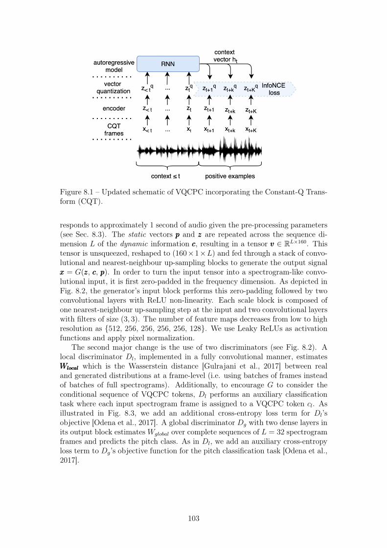
Figure 8.1 – Updated schematic of VQCPC incorporating the Constant-Q Trans-form (CQT).

responds to approximately 1 second of audio given the pre-processing parameters(see Sec. 8.3). The static vectors ppp and zzz are repeated across the sequence di-mension L of the dynamic information ccc, resulting in a tensor vvv ∈ RL×160. Thistensor is unsqueezed, reshaped to (160×1×L) and fed through a stack of convo-lutional and nearest-neighbour up-sampling blocks to generate the output signalxxx = G(zzz, ccc, ppp). In order to turn the input tensor into a spectrogram-like convo-lutional input, it is first zero-padded in the frequency dimension. As depicted inFig. 8.2, the generator’s input block performs this zero-padding followed by twoconvolutional layers with ReLU non-linearity. Each scale block is composed ofone nearest-neighbour up-sampling step at the input and two convolutional layerswith filters of size (3, 3). The number of feature maps decreases from low to highresolution as {512, 256, 256, 256, 256, 128}. We use Leaky ReLUs as activationfunctions and apply pixel normalization.

The second major change is the use of two discriminators (see Fig. 8.2). Alocal discriminator Dl, implemented in a fully convolutional manner, estimatesWlocalWlocalWlocal which is the Wasserstein distance [Gulrajani et al., 2017] between realand generated distributions at a frame-level (i.e. using batches of frames insteadof batches of full spectrograms). Additionally, to encourage G to consider theconditional sequence of VQCPC tokens, Dl performs an auxiliary classificationtask where each input spectrogram frame is assigned to a VQCPC token cl. Asillustrated in Fig. 8.3, we add an additional cross-entropy loss term for Dl’sobjective [Odena et al., 2017]. A global discriminator Dg with two dense layers inits output block estimatesWglobal over complete sequences of L = 32 spectrogramframes and predicts the pitch class. As in Dl, we add an auxiliary cross-entropyloss term to Dg’s objective function for the pitch classification task [Odena et al.,2017].

103

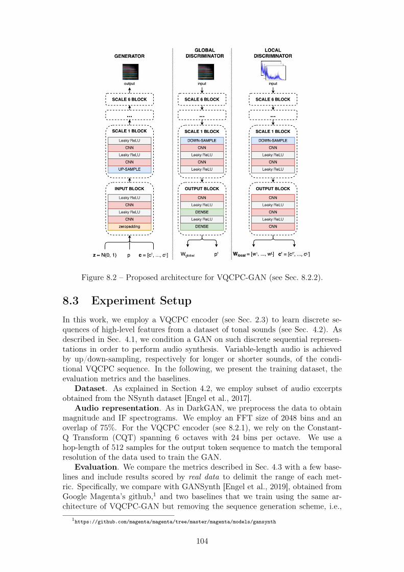
Figure 8.2 – Proposed architecture for VQCPC-GAN (see Sec. 8.2.2).

8.3 Experiment SetupIn this work, we employ a VQCPC encoder (see Sec. 2.3) to learn discrete se-quences of high-level features from a dataset of tonal sounds (see Sec. 4.2). Asdescribed in Sec. 4.1, we condition a GAN on such discrete sequential represen-tations in order to perform audio synthesis. Variable-length audio is achievedby up/down-sampling, respectively for longer or shorter sounds, of the condi-tional VQCPC sequence. In the following, we present the training dataset, theevaluation metrics and the baselines.

Dataset. As explained in Section 4.2, we employ subset of audio excerptsobtained from the NSynth dataset [Engel et al., 2017].

Audio representation. As in DarkGAN, we preprocess the data to obtainmagnitude and IF spectrograms. We employ an FFT size of 2048 bins and anoverlap of 75%. For the VQCPC encoder (see 8.2.1), we rely on the Constant-Q Transform (CQT) spanning 6 octaves with 24 bins per octave. We use ahop-length of 512 samples for the output token sequence to match the temporalresolution of the data used to train the GAN.

Evaluation. We compare the metrics described in Sec. 4.3 with a few base-lines and include results scored by real data to delimit the range of each met-ric. Specifically, we compare with GANSynth [Engel et al., 2019], obtained fromGoogle Magenta’s github,1 and two baselines that we train using the same ar-chitecture of VQCPC-GAN but removing the sequence generation scheme, i.e.,

1https://github.com/magenta/magenta/tree/master/magenta/models/gansynth

104

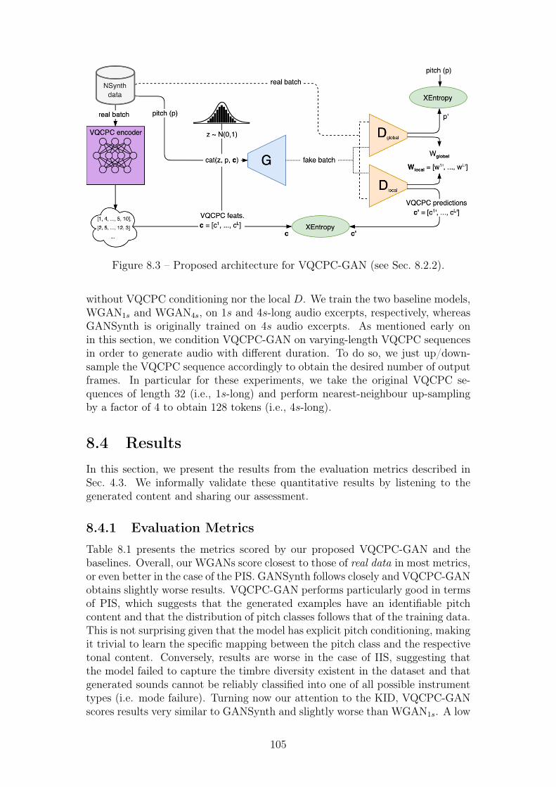
Figure 8.3 – Proposed architecture for VQCPC-GAN (see Sec. 8.2.2).

without VQCPC conditioning nor the local D. We train the two baseline models,WGAN1s and WGAN4s, on 1s and 4s-long audio excerpts, respectively, whereasGANSynth is originally trained on 4s audio excerpts. As mentioned early onin this section, we condition VQCPC-GAN on varying-length VQCPC sequencesin order to generate audio with different duration. To do so, we just up/down-sample the VQCPC sequence accordingly to obtain the desired number of outputframes. In particular for these experiments, we take the original VQCPC se-quences of length 32 (i.e., 1s-long) and perform nearest-neighbour up-samplingby a factor of 4 to obtain 128 tokens (i.e., 4s-long).

8.4 ResultsIn this section, we present the results from the evaluation metrics described inSec. 4.3. We informally validate these quantitative results by listening to thegenerated content and sharing our assessment.

8.4.1 Evaluation Metrics

Table 8.1 presents the metrics scored by our proposed VQCPC-GAN and thebaselines. Overall, our WGANs score closest to those of real data in most metrics,or even better in the case of the PIS. GANSynth follows closely and VQCPC-GANobtains slightly worse results. VQCPC-GAN performs particularly good in termsof PIS, which suggests that the generated examples have an identifiable pitchcontent and that the distribution of pitch classes follows that of the training data.This is not surprising given that the model has explicit pitch conditioning, makingit trivial to learn the specific mapping between the pitch class and the respectivetonal content. Conversely, results are worse in the case of IIS, suggesting thatthe model failed to capture the timbre diversity existent in the dataset and thatgenerated sounds cannot be reliably classified into one of all possible instrumenttypes (i.e. mode failure). Turning now our attention to the KID, VQCPC-GANscores results very similar to GANSynth and slightly worse than WGAN1s. A low

105

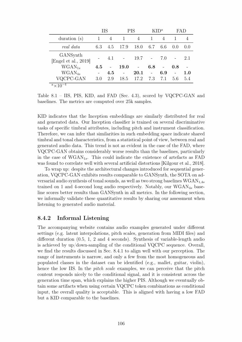
IIS PIS KIDa FADduration (s) 1 4 1 4 1 4 1 4

real data 6.3 4.5 17.9 18.0 6.7 6.6 0.0 0.0

GANSynth[Engel et al., 2019] - 4.1 - 19.7 - 7.0 - 2.1

WGAN1s 4.5 - 19.0 - 6.8 - 0.8 -WGAN4s - 4.5 - 20.1 - 6.9 - 1.0

VQCPC-GAN 3.0 2.9 18.5 17.2 7.3 7.1 5.6 5.4a×10−4

Table 8.1 – IIS, PIS, KID, and FAD (Sec. 4.3), scored by VQCPC-GAN andbaselines. The metrics are computed over 25k samples.

KID indicates that the Inception embeddings are similarly distributed for realand generated data. Our Inception classifier is trained on several discriminativetasks of specific timbral attributes, including pitch and instrument classification.Therefore, we can infer that similarities in such embedding space indicate sharedtimbral and tonal characteristics, from a statistical point of view, between real andgenerated audio data. This trend is not as evident in the case of the FAD, whereVQCPC-GAN obtains considerably worse results than the baselines, particularlyin the case of WGAN1s. This could indicate the existence of artefacts as FADwas found to correlate well with several artificial distortions [Kilgour et al., 2018].

To wrap up: despite the architectural changes introduced for sequential gener-ation, VQCPC-GAN exhibits results comparable to GANSynth, the SOTA on ad-versarial audio synthesis of tonal sounds, as well as two strong baselines WGAN1,4s

trained on 1 and 4-second long audio respectively. Notably, our WGAN4s base-line scores better results than GANSynth in all metrics. In the following section,we informally validate these quantitative results by sharing our assessment whenlistening to generated audio material.

8.4.2 Informal Listening

The accompanying website contains audio examples generated under differentsettings (e.g. latent interpolations, pitch scales, generation from MIDI files) anddifferent duration (0.5, 1, 2 and 4 seconds). Synthesis of variable-length audiois achieved by up/down-sampling of the conditional VQCPC sequence. Overall,we find the results discussed in Sec. 8.4.1 to align well with our perception. Therange of instruments is narrow, and only a few from the most homogeneous andpopulated classes in the dataset can be identified (e.g., mallet, guitar, violin),hence the low IIS. In the pitch scale examples, we can perceive that the pitchcontent responds nicely to the conditional signal, and it is consistent across thegeneration time span, which explains the higher PIS. Although we eventually ob-tain some artifacts when using certain VQCPC token combinations as conditionalinput, the overall quality is acceptable. This is aligned with having a low FADbut a KID comparable to the baselines.

106

8.5 ConclusionIn this work, we presented VQCPC-GAN, an adversarial model capable of per-forming variable-length sound synthesis of tonal sounds. We adapted the WGANarchitecture found in previous works [Engel et al., 2019, Nistal et al., 2020] to asequential setting by conducting two major architectural changes. First, we con-dition G on dynamic and static information captured, respectively, by a sequenceof discrete tokens learned through VQCPC, and a global noise zzz. Additionally, weintroduce a secondary fully-convolutional D that discriminates between real andfake data distributions at a frame level and predicts the VQCPC token associatedwith each frame. Results showed that VQCPC-GAN can generate variable-lengthsounds with controllable pitch content while still exhibiting results comparableto previous works generating audio with fixed-duration. We provide audio ex-amples in the accompanying website. As future work, we plan on investigatinghierarchical VQCPC tokens to condition the GAN on longer-term, compact rep-resentations of audio signals.

107

108

Chapter 9

Stochastic Restoration of HeavilyCompressed Musical Audio usingGANs

An exciting direction for future research is using GANs to learn rather complexmusical relationships between input-output audio pairs, e.g., generating a drumloop given some preexisting recording of a bass-line as musical context. This taskcan be framed as a domain translation problem. However, to train a GAN on sucha task, large amounts of multi-track musical audio data would be required, i.e., adataset where each of the individual audio tracks that compose a music piece isavailable as separate audio files. Gathering a large-scale dataset with such char-acteristics is challenging. Therefore, in this chapter, we address a pretext taskthat is simpler and for which we can create the audio data pairs artificially: audioenhancement of compressed musical audio. Initially, the audio enhancement fieldaimed to bridge legacy technologies for music storage, processing, and transmis-sion with current audio quality standards. Here we present a first attempt atlearning musical audio transformations with GANs by performing musical audiorestoration of heavily compressed MP3 music excerpts. We believe such a task isa feasible first step towards modeling more complex musical audio relationshipsin the future. An important reason is that we can artificially create the datasetby gathering high-quality musical audio and compressing it. Also, the task isconsiderably more straightforward than the end goal as the network is providedwith a denser context (the compressed audio data) while still exhibiting someof the fundamental challenges: generating some missing time-frequency contentthat is musically coherent with the conditional audio data.

The introduction of MP3 (i.e., MPEG-1 layer 3 [Brandenburg and Stoll, 1994])was transformative in how music was stored, transmitted, and shared in digitaldevices and on the internet. MP3 players, sharing platforms, and streamingresulted directly from the possibility to compress audio data without noticeableperceptual compromises. Compared to lossless audio coding formats, which allowfor a perfect reconstruction of the original PCM audio signal, lossy formats (likeMP3) typically lead to better compression by ignoring the parts of the signalto which humans are less sensitive. This process is also called perceptual codingwhich takes into account the physio- and psychological abilities of the humanauditory perception, resulting in so-called psychoacoustic models [Brandenburg,

109

1999].While several different lossy audio codecs (e.g., AAC, Opus, Vorbis, AMR)

exist, MP3 is undoubtedly the most commonly used. It is built upon an analy-sis filter bank and the modified discrete cosine transform (MDCT). In parallel,the signal is analyzed based on a perceptual model that exploits the psychoa-coustic phenomena of auditory masking to determine sound events in the audiosignal that are considered to be beyond human hearing capabilities. Based onthis information, the spectral components are quantized with specific resolutionand coded with variable bit allocation while keeping the noise introduced in thisprocess below the masking thresholds [Musmann, 2006]. This process may in-troduce a variety of deficiencies when configured with incorrect or very extremeparameters. For example, under large compression rates, high-frequency con-tent is susceptible to being removed, resulting in a bandwidth loss. Pre-echoescan occur when decoding very sudden sound events for which the quantizationnoise spreads out over the synthesis window and consequently precede the eventcausing the noise. Other common artifacts are so-called swirlies [Corbett, 2012],characterized by fast energy fluctuations in the low-level frequency content of thesound. Furthermore, there are other problems related to MP3 compression suchas double-speak as well as a general loss of transient definition, transparency, lossof detail clarity, and more [Corbett, 2012].

Many works exist which tackle the problem of audio enhancement, includingthe removal of compression artifacts. The most common recent methods usedfor these types of problems are based on deep learning. Typically, they focuson specific types of impairments present in the audio signals (e.g., reverberation[Williamson and Wang, 2017], bandwidth loss [Kumar et al., 2020], or audio codecartifacts [Zhao et al., 2019, Fisher and Scherlis, 2016, Skoglund and Valin, 2020,Biswas and Jia, 2020, Porov et al., 2018]). Also, different types of neural networkarchitectures have been studied for these tasks. For example, Convolutional Neu-ral Networks (CNNs) [Park and Lee, 2017], WaveNet-like architectures [Fisherand Scherlis, 2016, Gupta et al., 2019], and UNets [Isik et al., 2020, Hu et al.,2020]. However, most of the works in this line of research tackle the enhancementof speech signals [Zhao et al., 2019, Skoglund and Valin, 2020, Gupta et al., 2019,Biswas and Jia, 2020, Fisher and Scherlis, 2016, Park and Lee, 2017, Kontio et al.,2007, Isik et al., 2020, Hu et al., 2020, Li and Lee, 2015, Xu et al., 2015], andonly a few publications exist for musical audio restoration [Lagrange and Gon-tier, 2020, Miron and Davies, 2018, Porov et al., 2018, Deng et al., 2020]. Giventhe wide range of speech enhancement techniques in telephony, automatic speechrecognition, and hearing aids, this focus on speech is understandable. Also, com-pared to musical audio signals, speech signals are easier to study, as they are morehomogeneous, narrow-band, and usually monophonic. In contrast, musical audiosignals, particularly in the popular music genre, are highly varied. It typicallyconsists of multiple superimposed sources, which can be of any type, including(polyphonic) tonal instruments, percussion, (singing) voice, and various sound ef-fects. In addition, music is typically broad-band, containing frequencies spanningover the entire human hearing range.

Given that studies on deep learning-driven audio codec artifact removal formusical audio data are underrepresented in audio enhancement research, in thiswork, we attempt to provide some more insights into this task. We investigate the

110

limits of a generative neural network model when dealing with a general popularmusic corpus comprising music released in the last seven decades. In particu-lar, we are interested in the ability of the model to regenerate lost informationof heavily compressed musical audio signals using a stochastic generator (whichis not very common in audio enhancement, with [Biswas and Jia, 2020, Maitiand Mandel, 2019] being some exceptions). This work is not only relevant forthe restoration of MP3 data in existing (older) music collections. In the light ofcurrent developments in musical audio generation, where full songs can alreadybe generated from scratch [Dhariwal et al., 2020], musical audio enhancementmay soon possess a much more generative aspect. It has already been shown thatstrong generative models can enhance heavily corrupted speech through resynthe-sis with neural vocoders [Maiti and Mandel, 2019]. Along these lines, examininga generative (i.e., stochastic) decoder for heavily compressed audio signals maycontribute to insights about more efficient musical data storage and transmission.Today, music streaming is increasingly common, which poses issues regarding en-ergy consumption and environmental sustainability. When accepting deviationsfrom the original recording, higher compression rates could be reached with agenerative decoder without perceptual compromises in the listening experience.Moreover, there is no single best solution for heavily compressed audio signals torecover the original version. Therefore, it may be interesting for users to generatemultiple recoveries and pick the one they like most.

We introduce a Generative Adversarial Network (GAN) [Goodfellow et al.,2014] architecture for the restoration of MP3-encoded musical audio signals. Wetrain different stochastic (with z ∼ N (µ = 0, σ2 = I) input) and deterministicgenerators on MP3s with different compression rates. Using these models, we in-vestigate if 1) restorations of the models considerably improve the MP3 versions,2) if we can systematically pick samples among the outputs of the stochasticgenerators which are closer to the original in comparison to samples drawn fromthe deterministic generators, and 3) if the stochastic generators generally outputhigher-quality restorations than the deterministic generators. To that end, weperform an extensive evaluation of the different experiment setups utilizing ob-jective metrics and listening tests. We find that the models are successful in points1 and 2, but the random outputs of the stochastic generators are approximatelyon par (i.e., do not improve) the overall quality compared to the deterministicmodels (point 3).

The content of this chapter is extracted from our paper:

Lattner, S., and Nistal, J. “Stochastic Restoration of Heavily Com-pressed Musical Audio Using Generative Adversarial Networks.” MDPI,Electronics 10, no. 11: 1349, 2021.

The rest of this chapter is organized as follows. In Section 9.1 we revise pre-vious works in bandwidth extension and audio enhancement. In Section 9.2 weprovide a brief description of the proposed GAN architecture and the experimen-tal setup. Finally, in Section 9.3 we present and discuss the results and concludewith suggestions for future work in Section 9.4. Audio examples of the work areprovided in the accompanying website.1

1https://sonycslparis.github.io/restoration_mdpi_suppl_mat/

111

9.1 Related WorkThis work employs Generative Adversarial Networks (GANs) to restore MP3-compressed musical audio signals to their original high-quality versions. Thistask falls into the intersection of audio enhancement and bandwidth extension.Therefore, we review works on both these domains.

9.1.1 Bandwidth Extension

Low-resolution audio data (i.e., audio signals with a sample rate lower than44.1kHz) is generally preferable for storage or transmission over band-limitedchannels, like streaming music over the internet. Also, lossy audio encoders cansignificantly reduce the amount of information by removing high-frequency con-tent, but at the expense of potentially hampering the perceived audio quality.In order to restore the quality of such truncated audio signals, bandwidth exten-sion (BWE) methods aim to reconstruct the missing high-frequency content ofan audio signal given its low-frequency content as input [Larsen and Aarts, 2005].BWE is alternatively referred to as audio re-sampling or sample-rate conversionin the field of Digital Signal Processing (DSP), or as audio super-resolution inthe Machine Learning (ML) literature. Methods for BWE have been extensivelystudied in areas like audio streaming and restoration, mainly for legacy speechtelephony communication systems [Bansal et al., 2005, Gupta et al., 2019, Kontioet al., 2007, Li and Lee, 2015] or, less commonly, for degraded musical material[Lagrange and Gontier, 2020, Miron and Davies, 2018].

Pioneering works to speech BWE were originally algorithmic and operatedbased on a source-filter model. In such approaches, the problem of regenerat-ing a wide-band signal is divided into finding an upper-band source and thecorresponding spectral envelope, or filter, for that upper band. While methodsfor source generation were based on simple modulation techniques such as spec-tral folding and translation of a so-called low-resolution baseband [Makhoul andBerouti, 1979], the efforts focused on estimating the filter or spectral envelope[Dietz et al., 2002]. These works introduced the so-called spectral band replica-tion (SBR) method, where the lower frequencies of the magnitude spectra areduplicated, transposed, and adjusted to fit the high-frequency content. Becausein most use-cases for speech BWE the full transmission stack is controlled, most ofthese algorithmic methods rely on side information about the spectral envelope,obtained at the encoder from the full wide-band signal, and then transmittedwithin the bitstream for subsequent reconstruction at the decoder.

Learning-based approaches to speech BWE rely on large models to learn de-pendencies across the lower and higher end of the frequency spectrum, reducingthe need for side information in the transmitted bitstream (i.e., blind BWE).Methods based on Non-negative Matrix Factorization (NMF) treat the spectro-gram as a fixed set of non-negative bases learned from wide-band signals [Bansalet al., 2005]. These bases are fixed at test time and used to estimate the ac-tivation coefficients that best explain the narrow-band signal. The wide-bandsignal is then reconstructed by a linear combination of the base vectors weightedby the activations. These methods efficiently up-sample speech audio signals upto 22.05kHz but are sensitive to non-linear distortions due to the linear-mixing

112

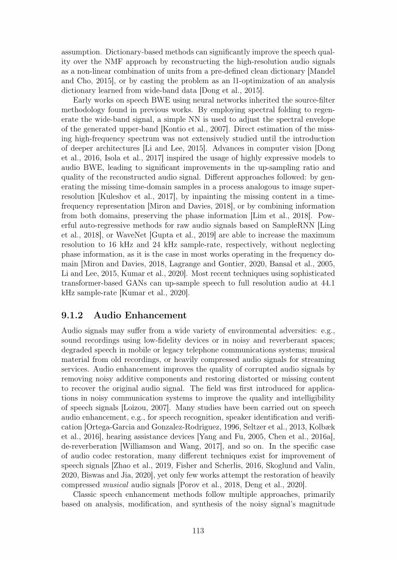
assumption. Dictionary-based methods can significantly improve the speech qual-ity over the NMF approach by reconstructing the high-resolution audio signalsas a non-linear combination of units from a pre-defined clean dictionary [Mandeland Cho, 2015], or by casting the problem as an l1-optimization of an analysisdictionary learned from wide-band data [Dong et al., 2015].

Early works on speech BWE using neural networks inherited the source-filtermethodology found in previous works. By employing spectral folding to regen-erate the wide-band signal, a simple NN is used to adjust the spectral envelopeof the generated upper-band [Kontio et al., 2007]. Direct estimation of the miss-ing high-frequency spectrum was not extensively studied until the introductionof deeper architectures [Li and Lee, 2015]. Advances in computer vision [Donget al., 2016, Isola et al., 2017] inspired the usage of highly expressive models toaudio BWE, leading to significant improvements in the up-sampling ratio andquality of the reconstructed audio signal. Different approaches followed: by gen-erating the missing time-domain samples in a process analogous to image super-resolution [Kuleshov et al., 2017], by inpainting the missing content in a time-frequency representation [Miron and Davies, 2018], or by combining informationfrom both domains, preserving the phase information [Lim et al., 2018]. Pow-erful auto-regressive methods for raw audio signals based on SampleRNN [Linget al., 2018], or WaveNet [Gupta et al., 2019] are able to increase the maximumresolution to 16 kHz and 24 kHz sample-rate, respectively, without neglectingphase information, as it is the case in most works operating in the frequency do-main [Miron and Davies, 2018, Lagrange and Gontier, 2020, Bansal et al., 2005,Li and Lee, 2015, Kumar et al., 2020]. Most recent techniques using sophisticatedtransformer-based GANs can up-sample speech to full resolution audio at 44.1kHz sample-rate [Kumar et al., 2020].

9.1.2 Audio Enhancement

Audio signals may suffer from a wide variety of environmental adversities: e.g.,sound recordings using low-fidelity devices or in noisy and reverberant spaces;degraded speech in mobile or legacy telephone communications systems; musicalmaterial from old recordings, or heavily compressed audio signals for streamingservices. Audio enhancement improves the quality of corrupted audio signals byremoving noisy additive components and restoring distorted or missing contentto recover the original audio signal. The field was first introduced for applica-tions in noisy communication systems to improve the quality and intelligibilityof speech signals [Loizou, 2007]. Many studies have been carried out on speechaudio enhancement, e.g., for speech recognition, speaker identification and verifi-cation [Ortega-Garcia and Gonzalez-Rodriguez, 1996, Seltzer et al., 2013, Kolbæket al., 2016], hearing assistance devices [Yang and Fu, 2005, Chen et al., 2016a],de-reverberation [Williamson and Wang, 2017], and so on. In the specific caseof audio codec restoration, many different techniques exist for improvement ofspeech signals [Zhao et al., 2019, Fisher and Scherlis, 2016, Skoglund and Valin,2020, Biswas and Jia, 2020], yet only few works attempt the restoration of heavilycompressed musical audio signals [Porov et al., 2018, Deng et al., 2020].

Classic speech enhancement methods follow multiple approaches, primarilybased on analysis, modification, and synthesis of the noisy signal’s magnitude

113

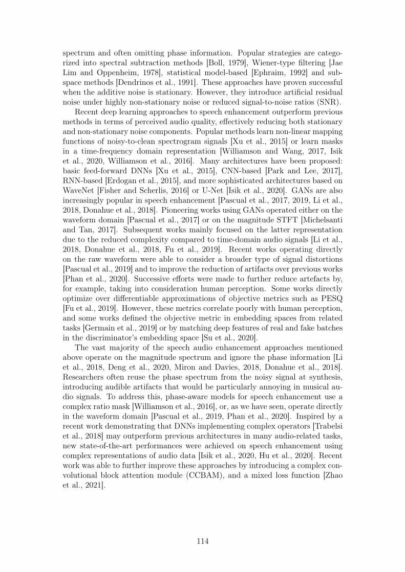
spectrum and often omitting phase information. Popular strategies are catego-rized into spectral subtraction methods [Boll, 1979], Wiener-type filtering [JaeLim and Oppenheim, 1978], statistical model-based [Ephraim, 1992] and sub-space methods [Dendrinos et al., 1991]. These approaches have proven successfulwhen the additive noise is stationary. However, they introduce artificial residualnoise under highly non-stationary noise or reduced signal-to-noise ratios (SNR).

Recent deep learning approaches to speech enhancement outperform previousmethods in terms of perceived audio quality, effectively reducing both stationaryand non-stationary noise components. Popular methods learn non-linear mappingfunctions of noisy-to-clean spectrogram signals [Xu et al., 2015] or learn masksin a time-frequency domain representation [Williamson and Wang, 2017, Isiket al., 2020, Williamson et al., 2016]. Many architectures have been proposed:basic feed-forward DNNs [Xu et al., 2015], CNN-based [Park and Lee, 2017],RNN-based [Erdogan et al., 2015], and more sophisticated architectures based onWaveNet [Fisher and Scherlis, 2016] or U-Net [Isik et al., 2020]. GANs are alsoincreasingly popular in speech enhancement [Pascual et al., 2017, 2019, Li et al.,2018, Donahue et al., 2018]. Pioneering works using GANs operated either on thewaveform domain [Pascual et al., 2017] or on the magnitude STFT [Michelsantiand Tan, 2017]. Subsequent works mainly focused on the latter representationdue to the reduced complexity compared to time-domain audio signals [Li et al.,2018, Donahue et al., 2018, Fu et al., 2019]. Recent works operating directlyon the raw waveform were able to consider a broader type of signal distortions[Pascual et al., 2019] and to improve the reduction of artifacts over previous works[Phan et al., 2020]. Successive efforts were made to further reduce artefacts by,for example, taking into consideration human perception. Some works directlyoptimize over differentiable approximations of objective metrics such as PESQ[Fu et al., 2019]. However, these metrics correlate poorly with human perception,and some works defined the objective metric in embedding spaces from relatedtasks [Germain et al., 2019] or by matching deep features of real and fake batchesin the discriminator’s embedding space [Su et al., 2020].

The vast majority of the speech audio enhancement approaches mentionedabove operate on the magnitude spectrum and ignore the phase information [Liet al., 2018, Deng et al., 2020, Miron and Davies, 2018, Donahue et al., 2018].Researchers often reuse the phase spectrum from the noisy signal at synthesis,introducing audible artifacts that would be particularly annoying in musical au-dio signals. To address this, phase-aware models for speech enhancement use acomplex ratio mask [Williamson et al., 2016], or, as we have seen, operate directlyin the waveform domain [Pascual et al., 2019, Phan et al., 2020]. Inspired by arecent work demonstrating that DNNs implementing complex operators [Trabelsiet al., 2018] may outperform previous architectures in many audio-related tasks,new state-of-the-art performances were achieved on speech enhancement usingcomplex representations of audio data [Isik et al., 2020, Hu et al., 2020]. Recentwork was able to further improve these approaches by introducing a complex con-volutional block attention module (CCBAM), and a mixed loss function [Zhaoet al., 2021].

114

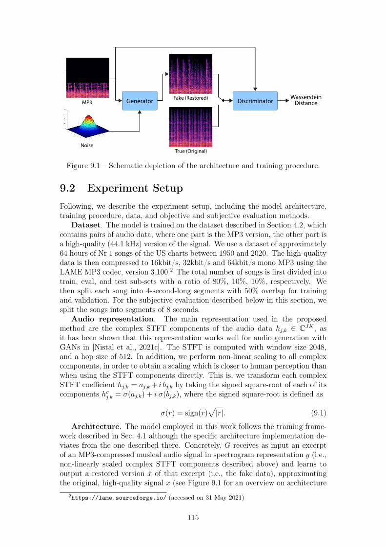
Generator DiscriminatorWasserstein

Distance

True (Original)

Fake (Restored)MP3

Noise

Figure 9.1 – Schematic depiction of the architecture and training procedure.

9.2 Experiment SetupFollowing, we describe the experiment setup, including the model architecture,training procedure, data, and objective and subjective evaluation methods.

Dataset. The model is trained on the dataset described in Section 4.2, whichcontains pairs of audio data, where one part is the MP3 version, the other part isa high-quality (44.1 kHz) version of the signal. We use a dataset of approximately64 hours of Nr 1 songs of the US charts between 1950 and 2020. The high-qualitydata is then compressed to 16kbit/s, 32kbit/s and 64kbit/s mono MP3 using theLAME MP3 codec, version 3.100.2 The total number of songs is first divided intotrain, eval, and test sub-sets with a ratio of 80%, 10%, 10%, respectively. Wethen split each song into 4-second-long segments with 50% overlap for trainingand validation. For the subjective evaluation described below in this section, wesplit the songs into segments of 8 seconds.

Audio representation. The main representation used in the proposedmethod are the complex STFT components of the audio data hj,k ∈ CJK , asit has been shown that this representation works well for audio generation withGANs in [Nistal et al., 2021c]. The STFT is computed with window size 2048,and a hop size of 512. In addition, we perform non-linear scaling to all complexcomponents, in order to obtain a scaling which is closer to human perception thanwhen using the STFT components directly. This is, we transform each complexSTFT coefficient hj,k = aj,k + i bj,k by taking the signed square-root of each of itscomponents hσj,k = σ(aj,k) + i σ(bj,k), where the signed square-root is defined as

σ(r) = sign(r)√|r|. (9.1)

Architecture. The model employed in this work follows the training frame-work described in Sec. 4.1 although the specific architecture implementation de-viates from the one described there. Concretely, G receives as input an excerptof an MP3-compressed musical audio signal in spectrogram representation y (i.e.,non-linearly scaled complex STFT components described above) and learns tooutput a restored version x of that excerpt (i.e., the fake data), approximatingthe original, high-quality signal x (see Figure 9.1 for an overview on architecture

2https://lame.sourceforge.io/ (accessed on 31 May 2021)

115

and training). D learns to distinguish between such restorations x and origi-nal high-quality versions of the signal x (i.e., the true data). In addition to thetrue/fake data, D also receives the MP3 versions of the respective excerpts. Thatway, it is ensured that the information present in the MP3 data is faithfully pre-served in the output of G. We test stochastic and deterministic generators inour experiments. For the stochastic models, we also provide some noise inputz ∼ N (0, I), resulting in different restorations for a given MP3 input, whereas forthe deterministic models we only provide the compressed audio. As the trainingcriterion, we use the WGAN loss [Arjovsky et al., 2017] described in Sec. 2.1.4.The full architecture is described in Table 9.1. Both G and D are based on di-lated convolutions with skip connections, combined with a novel concept which wecall Frequency Aggregation Filters. These are convolutional filters spanning thewhole frequency range, which contribute to the stability of the training and con-stitute a consequent take on the problem of non-local correlations in the frequencyspectrum. We also find that using so-called self-gating considerably reduces thememory requirement of the architecture by halving the number of input maps toeach convolutional layer without degradation of the results. In order to preventmode collapse, we propose a regularization that enforces a correlation betweendifferences in the noise input and differences in the model output. As opposedto most other works (but in line with our previous work [Nistal et al., 2021c]and other U-Net-based architectures [Isik et al., 2020, Hu et al., 2020]), we in-put (and output) directly the (non-linearly scaled) complex-valued spectrum tothe generator, eliminating the need to deal with phase information separately.For further details about the architecture, we encourage the reader to revise ouroriginal paper [Lattner and Nistal, 2021].

Training. Each model is trained for 40k iterations and a batch size of 12,which takes about 2 days on two NVIDIA Titan RTX with 24GB memory each.We use the ADAM optimizer [Kingma and Ba, 2015] with a learning rate of 1e-3and gradient penalty loss, to restrict the gradients of D to 1 Lipschitz [Gulrajaniet al., 2017]. We also use a loss term that penalizes the magnitudes of the outputof D for real input data, preventing the loss from drifting.

Evaluation. For this specific work, we deviate from the evaluation method-ology presented in Sec. 4.3. The main goal here is to assess the similarity betweenthe reference signals (i.e., the high-quality signals) and the signal approximations(i.e., MP3 versions of the audio excerpts or outputs of the proposed model). Theemployed objective metrics are standard in the audio enhancement literature:Log-Spectral Distance (LSD), Mean Squared Error (MSE), Signal-to-Noise Ratio(SNR), Objective Difference Grade (ODG), and Distortion Index (DI). We alsoperform a subjective evaluation in the form of the Mean Opinion Score (MOS).

• Objective Difference Grade and Distortion Index. The ObjectiveDifference Grade (ODG) is a computational approximation to subjectiveevaluations (i.e., the subjective difference grade) of users when comparingtwo signals. It ranges from 0 to −4, where lower values denote worse sim-ilarities between the signals. The Distortion Index (DI) is a metric thatis differently scaled but correlated to the ODG and can be seen as theamount of distortion between two signals. Both the ODG and DI are basedon a highly non-linear psychoacoustic model, including filtering and mask-ing to approximate the human auditory perception. They are part of the

116

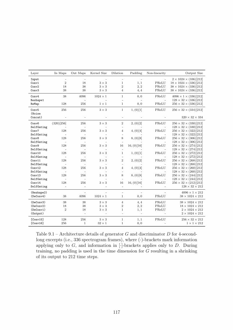
Layer In Maps Out Maps Kernel Size Dilation Padding Non-linearity Output Size

Input - - - - - - 2× 1024× (336)[212]Conv1 2 18 3× 3 1 1, 1 PReLU 18× 1024× (336)[212]Conv2 18 38 3× 3 2 2, 2 PReLU 38× 1024× (336)[212]Conv3 38 38 3× 3 4 4, 4 PReLU 38× 1024× (336)[212]

Conv4 38 4096 1024× 1 1 0, 0 PReLU 4096× 1× (336)[212]Reshape1 - - - - - 128× 32× (336)[212]ReMap 128 256 1× 1 1 0, 0 PReLU 256× 32× (336)[212]

Conv5 256 256 3× 3 1 1, (0)[1] PReLU 256× 32× (334)[212](NoiseConcat) - - - - - - 320× 32× 334

Conv6 (320)[256] 256 3× 3 2 2, (0)[2] PReLU 256× 32× (330)[212]SelfGating - - - - - - 128× 32× (330)[212]Conv7 128 256 3× 3 4 4, (0)[4] PReLU 256× 32× (322)[212]SelfGating - - - - - - 128× 32× (322)[212]Conv8 128 256 3× 3 8 8, (0)[8] PReLU 256× 32× (306)[212]SelfGating - - - - - - 128× 32× (306)[212]Conv9 128 256 3× 3 16 16, (0)[16] PReLU 256× 32× (274)[212]SelfGating - - - - - - 128× 32× (274)[212]Conv10 128 256 3× 3 1 1, (0)[1] PReLU 256× 32× (272)[212]SelfGating - - - - - - 128× 32× (272)[212]Conv11 128 256 3× 3 2 2, (0)[2] PReLU 256× 32× (268)[212]SelfGating - - - - - - 128× 32× (268)[212]Conv12 128 256 3× 3 4 4, (0)[4] PReLU 256× 32× (260)[212]SelfGating - - - - - - 128× 32× (260)[212]Conv13 128 256 3× 3 8 8, (0)[8] PReLU 256× 32× (244)[212]SelfGating - - - - - - 128× 32× (244)[212]Conv14 128 256 3× 3 16 16, (0)[16] PReLU 256× 32× (212)[212]SelfGating - - - - - - 128× 32× 212

(Reshape2) - - - - - 4096× 1× 212(DeConv4) 38 4096 1024× 1 1 0, 0 PReLU 38× 1024× 212

(DeConv3) 38 38 3× 3 4 4, 4 PReLU 38× 1024× 212(DeConv2) 18 38 3× 3 2 2, 2 PReLU 18× 1024× 212(DeConv1) 2 18 3× 3 1 1, 1 PReLU 2× 1024× 212(Output) - - - - - 2× 1024× 212

[Conv15] 128 256 3× 3 1 1, 1 PReLU 256× 32× 212[Conv16] 256 1 32× 1 1 0, 0 - 1× 1× 212

Table 9.1 – Architecture details of generator G and discriminator D for 4-second-long excerpts (i.e., 336 spectrogram frames), where (·)-brackets mark informationapplying only to G, and information in [·]-brackets applies only to D. Duringtraining, no padding is used in the time dimension for G resulting in a shrinkingof its output to 212 time steps.

117

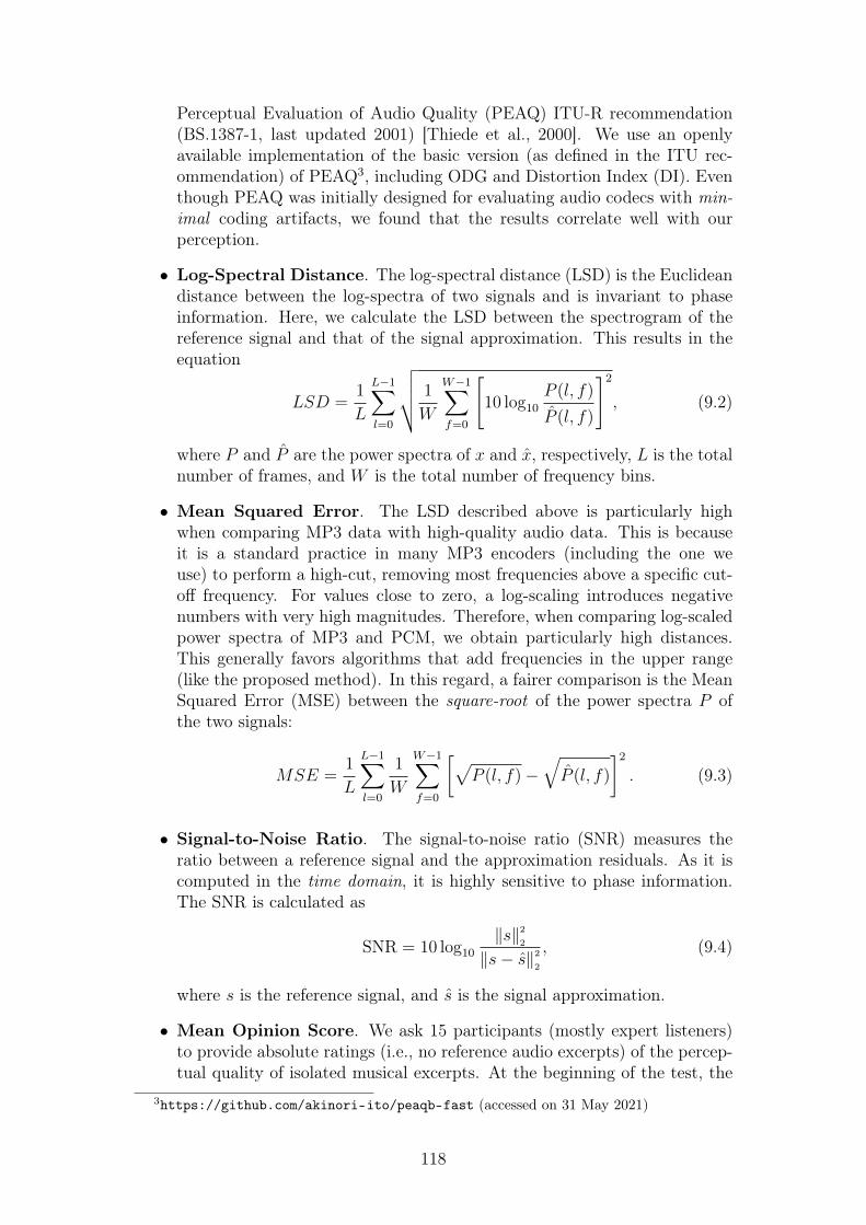
Perceptual Evaluation of Audio Quality (PEAQ) ITU-R recommendation(BS.1387-1, last updated 2001) [Thiede et al., 2000]. We use an openlyavailable implementation of the basic version (as defined in the ITU rec-ommendation) of PEAQ3, including ODG and Distortion Index (DI). Eventhough PEAQ was initially designed for evaluating audio codecs with min-imal coding artifacts, we found that the results correlate well with ourperception.

• Log-Spectral Distance. The log-spectral distance (LSD) is the Euclideandistance between the log-spectra of two signals and is invariant to phaseinformation. Here, we calculate the LSD between the spectrogram of thereference signal and that of the signal approximation. This results in theequation

LSD =1

L

L−1∑l=0

√√√√ 1

W

W−1∑f=0

[10 log10

P (l, f)

P (l, f)

]2, (9.2)

where P and P are the power spectra of x and x, respectively, L is the totalnumber of frames, and W is the total number of frequency bins.

• Mean Squared Error. The LSD described above is particularly highwhen comparing MP3 data with high-quality audio data. This is becauseit is a standard practice in many MP3 encoders (including the one weuse) to perform a high-cut, removing most frequencies above a specific cut-off frequency. For values close to zero, a log-scaling introduces negativenumbers with very high magnitudes. Therefore, when comparing log-scaledpower spectra of MP3 and PCM, we obtain particularly high distances.This generally favors algorithms that add frequencies in the upper range(like the proposed method). In this regard, a fairer comparison is the MeanSquared Error (MSE) between the square-root of the power spectra P ofthe two signals:

MSE =1

L

L−1∑l=0

1

W

W−1∑f=0

[√P (l, f)−

√P (l, f)

]2. (9.3)

• Signal-to-Noise Ratio. The signal-to-noise ratio (SNR) measures theratio between a reference signal and the approximation residuals. As it iscomputed in the time domain, it is highly sensitive to phase information.The SNR is calculated as

SNR = 10 log10

‖s‖22

‖s− s‖22

, (9.4)

where s is the reference signal, and s is the signal approximation.

• Mean Opinion Score. We ask 15 participants (mostly expert listeners)to provide absolute ratings (i.e., no reference audio excerpts) of the percep-tual quality of isolated musical excerpts. At the beginning of the test, the

3https://github.com/akinori-ito/peaqb-fast (accessed on 31 May 2021)

118

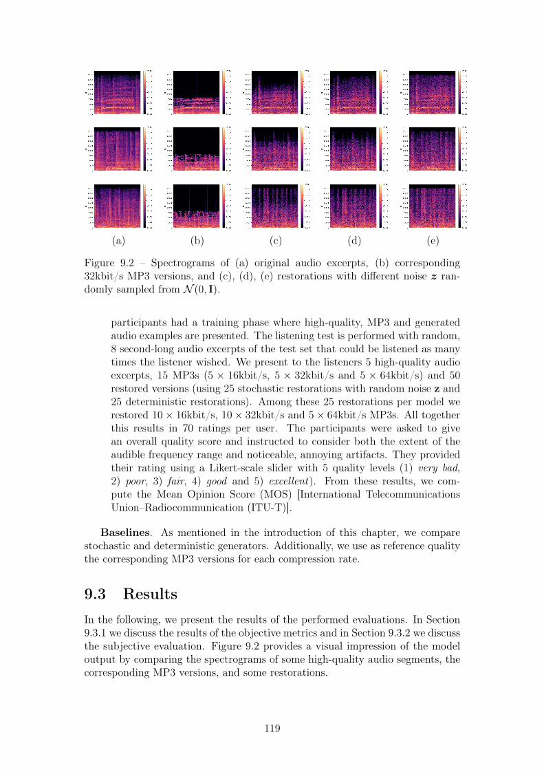
(a) (b) (c) (d) (e)

Figure 9.2 – Spectrograms of (a) original audio excerpts, (b) corresponding32kbit/s MP3 versions, and (c), (d), (e) restorations with different noise z ran-domly sampled from N (0, I).

participants had a training phase where high-quality, MP3 and generatedaudio examples are presented. The listening test is performed with random,8 second-long audio excerpts of the test set that could be listened as manytimes the listener wished. We present to the listeners 5 high-quality audioexcerpts, 15 MP3s (5 × 16kbit/s, 5 × 32kbit/s and 5 × 64kbit/s) and 50restored versions (using 25 stochastic restorations with random noise z and25 deterministic restorations). Among these 25 restorations per model werestored 10× 16kbit/s, 10× 32kbit/s and 5× 64kbit/s MP3s. All togetherthis results in 70 ratings per user. The participants were asked to givean overall quality score and instructed to consider both the extent of theaudible frequency range and noticeable, annoying artifacts. They providedtheir rating using a Likert-scale slider with 5 quality levels (1) very bad,2) poor, 3) fair, 4) good and 5) excellent). From these results, we com-pute the Mean Opinion Score (MOS) [International TelecommunicationsUnion–Radiocommunication (ITU-T)].

Baselines. As mentioned in the introduction of this chapter, we comparestochastic and deterministic generators. Additionally, we use as reference qualitythe corresponding MP3 versions for each compression rate.

9.3 ResultsIn the following, we present the results of the performed evaluations. In Section9.3.1 we discuss the results of the objective metrics and in Section 9.3.2 we discussthe subjective evaluation. Figure 9.2 provides a visual impression of the modeloutput by comparing the spectrograms of some high-quality audio segments, thecorresponding MP3 versions, and some restorations.

119

16k 32k 64kcompression rate

4.0

3.5

3.0

2.5

2.0

1.5

ODG

mp3 baselinestochasticdeterministic

16k 32k 64kcompression rate

3.5

3.0

2.5

2.0

1.5

1.0

0.5

0.0

0.5

1.0

DI

mp3 baselinestochasticdeterministic

16k 32k 64kcompression rate

2

3

5

10

LSD

mp3 baselinestochasticdeterministic

16k 32k 64kcompression rate

0

5

10

15

20

25

SNR

mp3 baselinestochasticdeterministic

Figure 9.3 – Violin plots of objective metrics for stochastic (sto), deterministic(det) models and MP3 baselines (mp3), for different compression rates (16 kbit/s,32kbit/s, 64kbit/s). Higher values are better for ODG, DI and SNR; lower valuesare better for LSD and MSE.

120

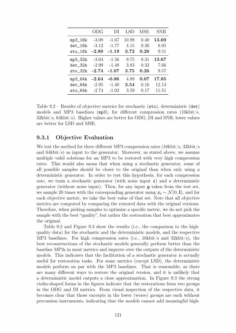
ODG DI LSD MSE SNR

mp3_16k -3.08 -1.67 10.98 0.40 13.69det_16k -3.12 -1.77 4.15 0.30 8.95sto_16k -2.80 -1.19 3.72 0.26 9.51

mp3_32k -3.04 -1.56 9.75 0.31 13.67det_32k -2.99 -1.48 3.83 0.32 7.66sto_32k -2.74 -1.07 3.75 0.26 9.57

mp3_64k -2.64 -0.86 4.89 0.07 17.85det_64k -2.95 -1.40 3.54 0.16 12.13sto_64k -2.74 -1.02 3.59 0.17 11.51

Table 9.2 – Results of objective metrics for stochastic (sto), deterministic (det)models and MP3 baselines (mp3), for different compression rates (16kbit/s,32kbit/s, 64kbit/s). Higher values are better for ODG, DI and SNR; lower valuesare better for LSD and MSE.

9.3.1 Objective Evaluation

We test the method for three different MP3 compression rates (16kbit/s, 32kbit/sand 64kbit/s) as input to the generator. Moreover, as stated above, we assumemultiple valid solutions for an MP3 to be restored with very high compressionrates. This would also mean that when using a stochastic generator, some ofall possible samples should be closer to the original than when only using adeterministic generator. In order to test this hypothesis, for each compressionrate, we train a stochastic generator (with noise input z) and a deterministicgenerator (without noise input). Then, for any input y taken from the test set,we sample 20 times with the corresponding generator using zi ∼ N (0, I), and foreach objective metric, we take the best value of that set. Note that all objectivemetrics are computed by comparing the restored data with the original versions.Therefore, when picking samples to optimize a specific metric, we do not pick thesample with the best “quality”, but rather the restoration that best approximatesthe original.

Table 9.2 and Figure 9.3 show the results (i.e., the comparison to the high-quality data) for the stochastic and the deterministic models, and the respectiveMP3 baselines. For high compression rates (i.e., 16kbit/s and 32kbit/s), thebest reconstructions of the stochastic models generally perform better than thebaseline MP3s in most metrics and improve over the outputs of the deterministicmodels. This indicates that the facilitation of a stochastic generator is actuallyuseful for restoration tasks. For some metrics (except LSD), the deterministicmodels perform on par with the MP3 baselines. That is reasonable, as thereare many different ways to restore the original version, and it is unlikely thata deterministic model outputs a close approximation. In Figure 9.3 the strongviolin-shaped forms in the figures indicate that the restorations form two groupsin the ODG and DI metrics. From visual inspection of the respective data, itbecomes clear that those excerpts in the lower (worse) groups are such withoutpercussion instruments, indicating that the models cannot add meaningful high-

121

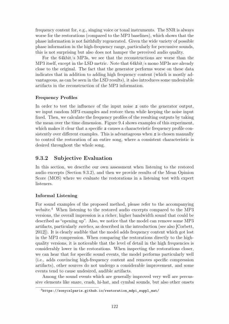
frequency content for, e.g., singing voice or tonal instruments. The SNR is alwaysworse for the restorations (compared to the MP3 baselines), which shows that thephase information is not faithfully regenerated. Given the wide variety of possiblephase information in the high-frequency range, particularly for percussive sounds,this is not surprising but also does not hamper the perceived audio quality.

For the 64kbit/s MP3s, we see that the reconstructions are worse than theMP3 itself, except in the LSD metric. Note that 64kbit/s mono MP3s are alreadyclose to the original. The fact that the generator performs worse on these dataindicates that in addition to adding high frequency content (which is mostly ad-vantageous, as can be seen in the LSD results), it also introduces some undesirableartifacts in the reconstruction of the MP3 information.

Frequency Profiles

In order to test the influence of the input noise z onto the generator output,we input random MP3 examples and restore them while keeping the noise inputfixed. Then, we calculate the frequency profiles of the resulting outputs by takingthe mean over the time dimension. Figure 9.4 shows examples of this experiment,which makes it clear that a specific z causes a characteristic frequency profile con-sistently over different examples. This is advantageous when z is chosen manuallyto control the restoration of an entire song, where a consistent characteristic isdesired throughout the whole song.

9.3.2 Subjective Evaluation

In this section, we describe our own assessment when listening to the restoredaudio excerpts (Section 9.3.2), and then we provide results of the Mean OpinionScore (MOS) where we evaluate the restorations in a listening test with expertlisteners.

Informal Listening

For sound examples of the proposed method, please refer to the accompanyingwebsite.4 When listening to the restored audio excerpts compared to the MP3versions, the overall impression is a richer, higher bandwidth sound that could bedescribed as “opening up”. Also, we notice that the model can remove some MP3artifacts, particularly swirlies, as described in the introduction (see also [Corbett,2012]). It is clearly audible that the model adds frequency content which got lostin the MP3 compression. When comparing the restorations directly to the high-quality versions, it is noticeable that the level of detail in the high frequencies isconsiderably lower in the restorations. When inspecting the restorations closer,we can hear that for specific sound events, the model performs particularly well(i.e., adds convincing high-frequency content and removes specific compressionartifacts), other sources do not undergo a considerable improvement, and someevents tend to cause undesired, audible artifacts.

Among the sound events which are generally improved very well are percus-sive elements like snare, crash, hi-hat, and cymbal sounds, but also other onsets

4https://sonycslparis.github.io/restoration_mdpi_suppl_mat/

122

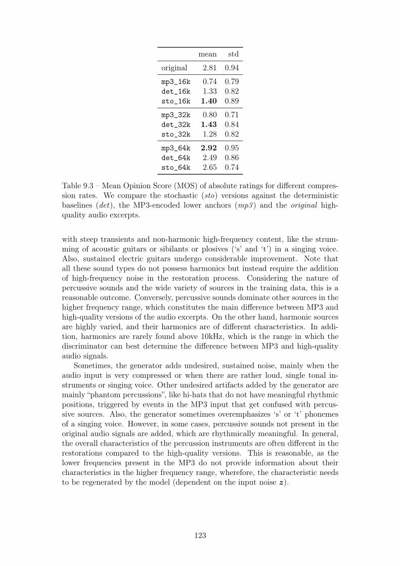
mean std

original 2.81 0.94

mp3_16k 0.74 0.79det_16k 1.33 0.82sto_16k 1.40 0.89

mp3_32k 0.80 0.71det_32k 1.43 0.84sto_32k 1.28 0.82

mp3_64k 2.92 0.95det_64k 2.49 0.86sto_64k 2.65 0.74

Table 9.3 – Mean Opinion Score (MOS) of absolute ratings for different compres-sion rates. We compare the stochastic (sto) versions against the deterministicbaselines (det), the MP3-encoded lower anchors (mp3 ) and the original high-quality audio excerpts.

with steep transients and non-harmonic high-frequency content, like the strum-ming of acoustic guitars or sibilants or plosives (‘s’ and ‘t’) in a singing voice.Also, sustained electric guitars undergo considerable improvement. Note thatall these sound types do not possess harmonics but instead require the additionof high-frequency noise in the restoration process. Considering the nature ofpercussive sounds and the wide variety of sources in the training data, this is areasonable outcome. Conversely, percussive sounds dominate other sources in thehigher frequency range, which constitutes the main difference between MP3 andhigh-quality versions of the audio excerpts. On the other hand, harmonic sourcesare highly varied, and their harmonics are of different characteristics. In addi-tion, harmonics are rarely found above 10kHz, which is the range in which thediscriminator can best determine the difference between MP3 and high-qualityaudio signals.

Sometimes, the generator adds undesired, sustained noise, mainly when theaudio input is very compressed or when there are rather loud, single tonal in-struments or singing voice. Other undesired artifacts added by the generator aremainly “phantom percussions”, like hi-hats that do not have meaningful rhythmicpositions, triggered by events in the MP3 input that get confused with percus-sive sources. Also, the generator sometimes overemphasizes ‘s’ or ‘t’ phonemesof a singing voice. However, in some cases, percussive sounds not present in theoriginal audio signals are added, which are rhythmically meaningful. In general,the overall characteristics of the percussion instruments are often different in therestorations compared to the high-quality versions. This is reasonable, as thelower frequencies present in the MP3 do not provide information about theircharacteristics in the higher frequency range, wherefore, the characteristic needsto be regenerated by the model (dependent on the input noise z).

123

Formal Listening

Table 9.3 shows the results of the listening test (i.e., MOS ratings). Overall,the original and the 64kbit/s MP3s (mp3_64k) obtain the highest ratings andthe restored 64kbit/s MP3s (det_64k and sto_64k) perform slightly worse. Theratings for the restored 16kbit/s and 32kbit/s (det_16k, sto_16k, det_32k andsto_32k) are considerably better than the MP3 versions (mp3_16k and mp3_-32k). This shows that the proposed restoration process indeed results in betterperceived audio quality. However, the random samples from the stochastic gen-erators are not assessed better than the outputs of the deterministic generators(the differences are not significant, as detailed below). We note that for the highcompression rates, we reach only about half the average rating of the high-qualityversions (but about double the rating of the MP3 versions). While overall, a re-stored MP3 version possesses a broader frequency range, weak ratings may resultfrom off-putting artifacts, like the above-mentioned “phantom percussions”. In 8-second-long excerpts, only one irritating artifact can already lead to a relativelyweak rating for the whole example.

As the variance of the ratings is rather high, we also compute t-tests for statis-tical significance comparing responses to the different stimuli. We obtain p-values< 0.05 (< 10−5) when comparing det and sto to mp3 for compression rates below64kbit/s. Conversely, we observe no statistically significant differences betweenratings of det and sto for all compression rates (p-values > 0.15). Responsesto original and mp3_64k also show no statistically significant differences (p-value= 0.49). We also observe no statistical significance between responses to mp3_64kand det_64k (p-value = 0.06), whereas there is a significant difference betweenratings of sto_64k and mp3_64k (p-value = 0.04).

9.4 ConclusionThis chapter presented a GAN architecture for the stochastic restoration of high-quality musical audio signals from highly compressed MP3 versions. We tested1) if the output of the proposed model improves the quality of the MP3 inputs,2) if a stochastic generator improves (i.e., can generate samples closer to theoriginal) over a deterministic generator, and 3) if the outputs of the stochasticvariants are generally of higher quality than deterministic baseline models.

Results show that the restorations of the highly compressed MP3 versions(16kbit/s and 32kbit/s) are generally better than the MP3 versions themselves,which is reflected in a thorough objective evaluation, and confirmed in percep-tual tests by human experts. We also tested weaker compression rates (64kbit/smono), where we found that the proposed architecture results in slightly worseresults than the MP3 baseline. We could also show in the objective metricsthat a stochastic generator can indeed output samples closer to the original thanwhen using a deterministic generator. However, the perceptual tests indicate thatwhen drawing random samples from the stochastic generator, the results are notassessed significantly better than the results of the deterministic generator.

Due to the wide variety of popular music, the task of generating missingcontent is very challenging. However, the proposed models succeeded in addinghigh-frequency content for particular sources resulting in an overall improved

124

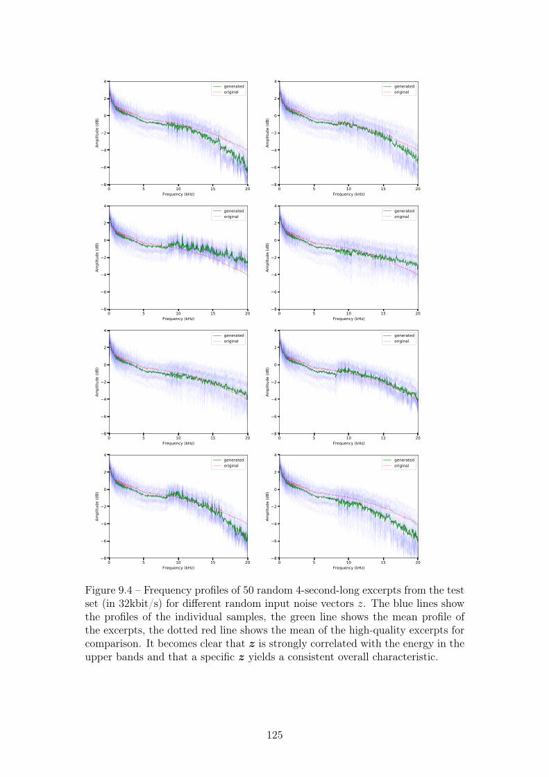
0 5 10 15 20Frequency (kHz)

8

6

4

2

0

2

4

Ampl

itude

(dB)

generatedoriginal

0 5 10 15 20Frequency (kHz)

8

6

4

2

0

2

4

Ampl

itude

(dB)

generatedoriginal

0 5 10 15 20Frequency (kHz)

8

6

4

2

0

2

4

Ampl

itude

(dB)

generatedoriginal

0 5 10 15 20Frequency (kHz)

8

6

4

2

0

2

4

Ampl

itude

(dB)

generatedoriginal

0 5 10 15 20Frequency (kHz)

8

6

4

2

0

2

4

Ampl

itude

(dB)

generatedoriginal

0 5 10 15 20Frequency (kHz)

8

6

4

2

0

2

4

Ampl

itude

(dB)

generatedoriginal

0 5 10 15 20Frequency (kHz)

8

6

4

2

0

2

4

Ampl

itude

(dB)

generatedoriginal

0 5 10 15 20Frequency (kHz)

8

6

4

2

0

2

4

Ampl

itude

(dB)

generatedoriginal

Figure 9.4 – Frequency profiles of 50 random 4-second-long excerpts from the testset (in 32kbit/s) for different random input noise vectors z. The blue lines showthe profiles of the individual samples, the green line shows the mean profile ofthe excerpts, the dotted red line shows the mean of the high-quality excerpts forcomparison. It becomes clear that z is strongly correlated with the energy in theupper bands and that a specific z yields a consistent overall characteristic.

125

perceived quality of the music. Examples for sources where the model clearlylearned to generate meaningful high-frequency content are percussive elements(i.e., snare, crash, hi-hat and cymbal sounds), sibilants or plosives ( ‘s’ and ‘t’) insinging voice, strummed acoustic guitars and (sustained) electric guitars. In thisregard, we believe that the results presented in this work show that GANs can bea promising avenue towards learning intricate relationships between input-outputmusical audio pairs.

We expect future improvements when limiting the style of the training datato particular genres or time periods of production. Also, as we use the complexspectrum directly, the adaption to Complex Networks [Trabelsi et al., 2018] couldimprove the results further. In order to tackle the problem of “phantom percus-sions” (as described in Section 9.3.2), a beat detection algorithm could provideadditional information to the generator so that it is better informed about therhythmic structure of the input. For improvement in learning to restore the har-monics of tonal sources, other representations (e.g., Magnitude and InstantaneousFrequencies (Mag-IF) [Engel et al., 2019]) or a different scaling (e.g., Mel-scaledspectrograms) could be tested for the input and output of the generator.

126

127

Chapter 10

On the Development and Practiceof AI Technology for ContemporaryPopular Music Production

The practice of music creation has since long involved instruments and, more gen-erally, technology. Breakthroughs and paradigm shifts resulting from the devel-opment of technology may significantly influence music-making practice (whichwe refer to as music production in this chapter). An example of this can bewitnessed in the early use of electronic equipment for musical purposes in therecording studios during the 1950s or the popularization of synthesizers in the1970s, allowing for artistic experimentation and enabling new ways to producemusic.

Introducing novel technologies into the music creation workflow is often acomplex process that initially requires specialists to take care of the technicalaspects. In the case of early recording studio technology, an example of this is thecollaboration between engineer Pierre Schaeffer and musician Pierre Henry, whoin the ’50s collaborated closely to find new musical applications of technology[Palombini, 1993]. Another example is the collaboration of analog synthesizerpioneer Robert Moog with several musicians [Pinch and Trocco, 2002]. Over time,the practice of music creation evolved to integrate new technologies, blurring thedistinction between engineer, musician, and music producer [Moorefield, 2005].In contemporary genres such as rap, dance, and, more generally, electronic music,technology has become such an integral part of the music that there is typicallyno meaningful distinction between the composition, recording, and production ofmusic.

Today, as shown in Chapters 2 and 3, advances in artificial intelligence (AI),and in particular machine learning, promise to have a profound transformativeeffect in music practice in general. However, AI-based technology appears tobe at the same stage as the recording studio was in the 1960s: the technologyexists, but making it available as a tool for music production generally requiresspecialists (AI engineers) operating the technology and assisting musicians in itsusage.

The process of technology becoming part of a new music practice does notsolely rely on engineering, nor is it a matter of taking inventory of artists’ needs as“user requirements" and fulfilling these requirements. The term musical research

128

has been proposed to denote this “co-adaptation" of technology and musical prac-tice [Cont, 2013]. Several research institutes are explicitly dedicated to this type ofresearch, such as the Institute for Research and Coordination in Acoustics/Music(IRCAM, Paris, France) or the Center for New Music and Audio Technologies(CNMAT, Berkeley, California). The Magenta Project at Google Brain, with itsfocus on AI-based music technology, contributes to musical research by makingthe technology widely available in the form of open-source software, and in somecases, sharing hardware prototypes of the technology with musicians [Engel et al.,2017].1

Sony CSL’s music team is a musical research lab developing AI-based tools forinnovation in music practice. At CSL, we believe that musicians and engineersworking in unison is a vital part of the innovation process for two main reasons.On the one hand, engineers may gain knowledge of what musicians look for artis-tically, and, on the other hand, musicians may become aware of the opportunitiesthe technology offers for novel music practices. In this chapter, we report onthe collaborations with professional musicians, in which they experiment withdifferent AI-based music tools developed at Sony CSL.

The content of this chapter is extracted from our paper:

Deruty, E., Grachteen, M., Lattner, S., Nistal, J., andAouameur, C.. “On the development and practice of AI technol-ogy for contemporary popular music production.” Transactions of theInternational Society for Music Information Retrieval (TISMIR), 2022.

The chapter is organized as follows. In Section 10.1 we describe the procedureunder which we collaborate with artists and provide a brief overview of the toolsused. In Section 10.2 we give an account of the artists’ feedback, categorizing howthey interact with the tools. Section 10.3 lists observations and lessons learnedthroughout such process, pointing out specific forms that the validation processof AI tools for music production may assume. Finally, in Section 10.4 we presentthe overall conclusions.

10.1 Experiment SetupAt the core of musical research is the interaction between artists and technology.At CSL, this interaction occurs in long-term collaborations with professional mu-sicians working in various musical genres, with a strong focus on recent populartrends. Over the past years, we tested our AI-driven music production prototypes(at different stages of development) with them.

The musicians we worked with include, in no particular order: songwrit-ers/producers Yann Macé and Luc Leroy, from company Hyper Music2; beat-maker/producer Twenty9, currently affiliated with Sony Music Publishing France;composer and conductor Uèle Lamore, currently affiliated with XXXIM / SonyMasterworks Berlin; Donn Healy, independent electronic music producer.

1https://nsynthsuper.withgoogle.com/2https://www.hyper-music.com/

129

10.1.1 Procedure

At the start of the collaboration, we give the artists an overview of AI and machinelearning applied to music and explain our vision of music AI as tools to enrichthe creative workflow in music production. We give them a demonstration of theavailable tool prototypes in the lab where they can try out the software. Whenthe artists are familiar with the ways the tools work, they use them in their ownworking environment, typically for several weeks or months, experimenting withthe tools in their music production process. Typically there are follow-up sessionswhere the artists talk of their experience, what they like about the tools, whatthey dislike, and what changes they would like to see. We gather such feedback inthe form of oral or written interviews, email exchanges, or presentations. Giventhe artist’s feedback, the tools are modified accordingly as long as changes canbe realized within a reasonable effort. Proposals that imply more fundamentalchanges to the tools are used to guide future development. When the artistshave finalized their work, they send us the outcomes and a description of theirworkflow, which typically includes the AI tools, along with several other musicproduction tools they work with.

10.1.2 Tools

The AI tools provided to the artists have been recently developed at our lab andare generally prototypes in the form of either standalone applications, VST plug-ins for digital audio workstations (DAW), or servers accessible through a webinterface. They cover different aspects of the music production process, rangingfrom sound design to mixing/equalization and melodic and rhythmic materialgeneration. The tools have been presented in more detail in prior publications,so here we provide only a brief introduction:

• Notono. An interactive tool for generating instrumental one-shots [Bazinet al., 2020]. It uses VAE architecture that operates on spectrograms andis conditioned on instrument labels. You can start from a sound you likeand interactively modify it by inpainting the spectrogram.

• Planet Drums, DrumGAN, Impact Drums. Three drum sound syn-thesizers. Planet Drums is based on a VAE architecture that allows theuser to explore different drum sounds by traversing a low-dimensional em-bedding of the latent space [Aouameur et al., 2019]. DrumGAN and ImpactDrums are based on GANs [Goodfellow et al., 2014]. DrumGAN is con-ditioned on perceptual features that can be used as controls [Nistal et al.,2020].

• DrumNet. A tool for creating drum tracks conditioned on existing audiotracks like guitar, bass, or keyboard tracks [Lattner and Grachten, 2019].The output adapts to the tempo and rhythm of the existing tracks, andusers can explore different rhythmic variations by traversing a latent space.

• BassNet/LeadNet. A tool for creating bass tracks (BassNet) or leadtracks (LeadNet), conditioned on one or more existing audio tracks [Grachtenet al., 2020]. The output adapts to the tonality of the existing tracks (if

130

the input is tonal), and users can explore different rhythmic and melodicvariations of the output by traversing a latent space. The model outputsboth MIDI and audio and conveys articulation, dynamics, timbre, and into-nation. In terms of model architecture, BassNet and LeadNet are identical.They differ in that BassNet was trained on bass guitar tracks, and LeadNetwas trained on vocal and lead guitar tracks.

• ResonanceEQ, ProfileEQ. Adaptive equalizers for audio mixing andmastering tasks [Grachten et al., 2019]. They consist of hand-designedprocessing pipelines to adjust the spectral characteristics of the sound adap-tively and other feed-forward convolutional neural networks to estimate op-timal control parameters for the equalizer process conditional on the inputaudio.

10.2 ResultsHaving introduced the artists we work with and the AI-driven prototypes theyuse, we will share some of their insights when producing music. We give them thefreedom to use the tools where and how they wish, without particular guidelinesor constraints. We identify and discuss some typical interaction patterns withthe tools. We then use the observations to critically assess current paradigmsand suggest improvements to the current state-of-the-art for interaction with AI-driven music production tools.

10.2.1 Push & Pull Interactions

In the field of creative text writing, two approaches to trigger the machine’soutput are described [Clark E. et al., 2018]: Push (automatically initiated) andPull (person-initiated). Artists often use push interactions when starting a musicpiece. Musician Twenty9 testifies:

“Flow Machines3 (FM) is a true source of inspiration at the startof the composition process, when I face a blank page. I let myselfbeing guided by what FM does. It allows me to spend less timeon the symbolic composition, more time on the sample design, andto have fresh ideas for the drums and the bass, to have fun on theprogramming without being tired by the symbolic composition."

This initial push suggestion triggers a sequence of pull interactions, wherethe artist refines the initial idea by feeding it back to the system and stitchingtogether new suggestions. Still according to Twenty9:

“I really liked the chord sequence generated by FM and mostly themelody too, with a few details ready [...] I interacted with FM torecompose parts of this 16 bars melody, until I could extract 4 barsthat I really liked. It was done very quickly!"

3https://www.flow-machines.com/

131

One particular case of pull is known as priming [Huang et al., 2020]: theartist designs an input to drive the generation process. This amounts to whatis referred to as dense conditioning [Grachten et al., 2020], where the output ofa model is controlled by providing a rich source of information (e.g. an audioor MIDI track) instead of sparser types of information that are provided by thetypical UI elements of a control panel (sliders, buttons, presets...). One exampleof the priming process used in production from Yann Macé:

“Made an 8-bar bounce with kick, snare plus a very simple legato basspart (not used thereafter). Fed this bounce to LeadNet. Tweakedaround until I hear something inspiring : it plays a cool part with a4-note hook that sounds good at the end of the chord cycle."

Note that BassNet, LeadNet, and DrumNet are designed to be conditionedon audio input, which has multiple advantages. First, it better integrates intomusic production workflows, as audio is more general than MIDI (one can alwaysrender MIDI to audio, but not the other way around). Second, audio is richer,as it combines both tonal information, expressivity, and timbral characteristics(including higher pitch resolution, without MIDI quantization). Third, it hasa higher potential to result in unexpected (but valuable) outputs, as audio cancarry much more variety than symbolic music representation. Donn Healy states:

“DrumNet handled this quirky input very well, it followed the expres-sion to a T [very precisely]",

which summarizes the points made above, namely expressivity, richness of theaudio input, and surprise when using "quirky" material.

10.2.2 On Machine Interference With the Creative Process

It has been noted before that AI-driven music tools can interfere with musicalgoals [Huang et al., 2020]. We have experienced that, even at early stages, proto-types require format compatibility (e.g., implementation as DAW plug-ins) andcompatibility with the artist’s method to actually be used.

Even then, artists may be reluctant to use technology proposing musical con-tent. However, doing so may be beneficial in terms of results. Twenty9 testifies:

“[...]. Since I was a fan of this loop [...] I went straight to drums.Honestly, in the euphoria, I wanted to jump on my usual sampler andset a rhythm in 5 min. I forced myself to confront DrumNet [...]. Tomy surprise, [...] I ended up with a pattern that worked well [eventhough] on my own I would not have placed my kicks like that."

“[Working with LeadNet], I am confronted with melodies that I wouldprobably never have thought of."

AI-based approaches interfere with creative goals because they disturb thepreconceived vision of the artist, and it is mostly a desirable design feature (asopposed to interference with the artist’s workflow). From artists’ feedback orfigures such as Moog and Schaeffer, we witness creativity emerging from the ma-chine’s interference. It remains the artist’s prerogative to set the right conditionsand remain attentive for interesting musical combinations.

132

10.2.3 Exploration and Higher-level Control

As witnessed by [Huang et al., 2020], many musicians adopted the generate-then-curate strategy when working with specific AI-driven prototypes; they firstgenerate many samples and then select those they deem valuable for further usage.Artist Uèle Lamore adopted such strategy when working with the prototypes:

“The goal was to generate a selection of percussion/drum samples thatI could see fit to use in any given setting. [...] generating percussionsounds with DrumGAN and Planet Drums. I’m not interested ingenerating sounds that sound like a "real" or "classic" kit. I wantsounds that are very abstract [...] I now had this selection of soundsavailable."

However, note that 1) such strategies are also common outside AI-based ap-proaches and that 2) AI appears to make such strategies more efficient. From ourobservations, a misconception seems to be that AI tools are doomed to spit outa lot of useless material, which then needs to be curated.

AI can potentially free artists from cumbersome workflows involving skip-ping through sample libraries or fiddling with numerous controls of a complexsynthesizer to realize an idea. In particular, when AI model engineering andhuman-computer interaction is developed further in unison, we expect to see ashift from the generate-then-curate strategy to a more efficient and creativelyenriching exploration and higher-level control paradigm. A prominent exampleof exploration in generative models is the navigation of latent spaces, where po-sitions and directions have intuitive meaning so that the desired solution can befound in a more controlled way [Nistal et al., 2020, Aouameur et al., 2019, En-gel et al., 2019]. Such higher-level control was also studied for the generation ofminute-long material [Lattner and Grachten, 2019, Grachten et al., 2020]. Notethat in these works, considerations about the user interaction was an integralpart of the model design process. Keeping the artist in mind in the early stagesof model engineering will increase user empowerment, efficiency, and satisfaction.

10.2.4 AI, the New Analog?

Musicians regularly take advantage of particular prototype behaviors that wouldnot be deemed acceptable in the context of scientific validation. Specifically,behaviors that (1) would be validated as incorrect (i.e., not complying with thetraining data set’s characteristic – “glitches"), or (2) stem from an abnormal usageof the model in which validation is not possible (e.g., out-of-domain input).

Glitches

Musicians sometimes point out that particular artifacts are great, that they havea distinct identity. Twenty9 speaks about the Impact Drums and Planet Drums’prototype:

“[...] I love [the artefacts’] color, it changes from what I hear in thecurrently available packs that do a lot of recycling. [...] Artistically,

133

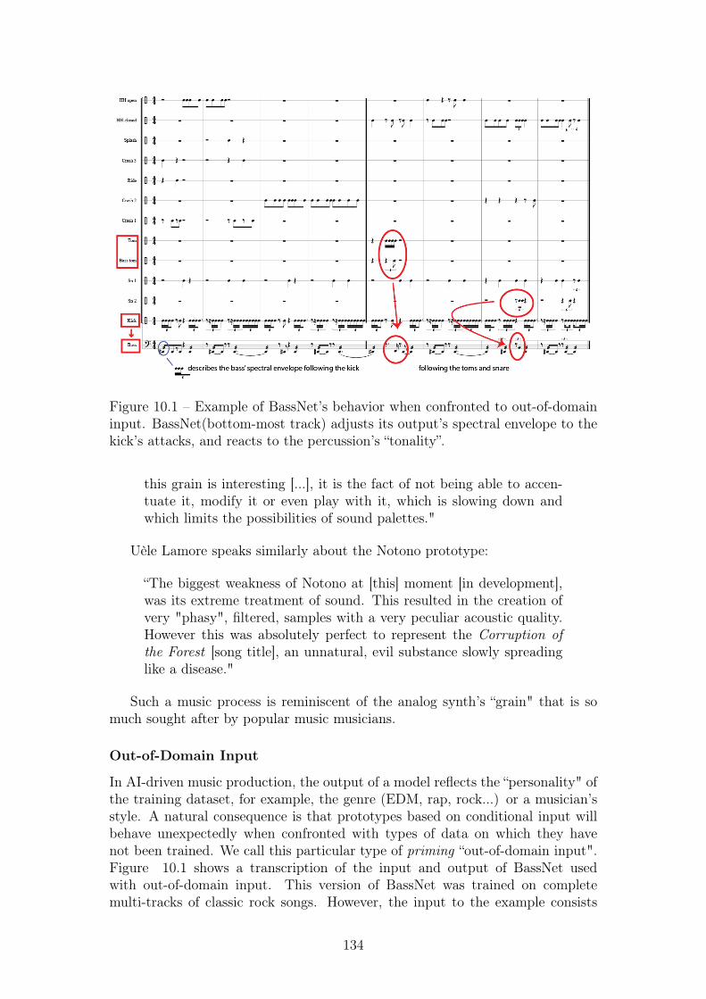
Figure 10.1 – Example of BassNet’s behavior when confronted to out-of-domaininput. BassNet(bottom-most track) adjusts its output’s spectral envelope to thekick’s attacks, and reacts to the percussion’s “tonality”.

this grain is interesting [...], it is the fact of not being able to accen-tuate it, modify it or even play with it, which is slowing down andwhich limits the possibilities of sound palettes."

Uèle Lamore speaks similarly about the Notono prototype:

“The biggest weakness of Notono at [this] moment [in development],was its extreme treatment of sound. This resulted in the creation ofvery "phasy", filtered, samples with a very peculiar acoustic quality.However this was absolutely perfect to represent the Corruption ofthe Forest [song title], an unnatural, evil substance slowly spreadinglike a disease."

Such a music process is reminiscent of the analog synth’s “grain" that is somuch sought after by popular music musicians.

Out-of-Domain Input

In AI-driven music production, the output of a model reflects the “personality" ofthe training dataset, for example, the genre (EDM, rap, rock...) or a musician’sstyle. A natural consequence is that prototypes based on conditional input willbehave unexpectedly when confronted with types of data on which they havenot been trained. We call this particular type of priming “out-of-domain input".Figure 10.1 shows a transcription of the input and output of BassNet usedwith out-of-domain input. This version of BassNet was trained on completemulti-tracks of classic rock songs. However, the input to the example consists

134

of the audio of death metal solo drums. BassNet (bottom-most track) adjustsits output’s spectral envelope to the kick’s attacks and reacts to the percussion’s“tonality," the toms, and the snare.

Uèle Lamore describes her experience with out-of-domain use of a version ofBassNet that was trained on mostly 4/4 beat rock, hip-hop, and EDM multi-tracks, always including a drum section:

“[...] none of my music on this EP is in 4/4, it’s as far as you can getfrom pop or hip-hop and this track had zero percussion at this point.As a result of this, BassNet did not behave the way you would expectit to. However, I had the pleasant surprise to see the generations wereperfect melodies that worked really well in this ambient setting."

Out-of-domain input is reminiscent of the exploratory use of the Moog syn-thesizer [Pinch and Trocco, 2002]. The model is considered a complex and un-predictable music generator whose output can be explored using proper triggers.Working with these tools becomes “a journey of discovery."

Out-of-Domain Output

We denote “out-of-domain output" when an artist uses the output of a tool for adifferent purpose than intended. For example, Donn Healy states:

“I took a new snare pattern that DrumNet suggested and I broughtit into a melodic Omnisphere sound, and I spread the notes in a waythat they told a musically cohesive story [..] I really enjoyed that."

Also, as illustrated by the Uèle Lamore’s quote above, some artists took out-puts of BassNet and pitched it to obtain melodies instead of bass lines. Similarly,we discovered that ResonanceEQ, a tool designed to remove resonances, is usuallyinverted by artists to add resonances to audio.

10.3 GuidesFinally, we want to communicate some of the lessons we learned throughout ourwork in AI-based musical research. They are meant to constitute some practicalguides to pushing research towards creating output that is useful in music produc-tion. AI-based musical research involves more than model design. It is stronglymulti-disciplinary, comprising, among other fields, user experience, and human-computer interaction, music and sound perception, musicology, studio production,and machine learning. With this in mind, we enumerate some “learned lessons,"which may guide the practical work in AI-based musical research (see Section10.3.1). Also, we provide some suggestions for validation in AI-based musicalresearch, which goes beyond typical model evaluation (see Section 10.3.2).

10.3.1 Lessons Learned on AI-based Musical Research

Considering musical research as the simultaneous practice of innovation in musictechnology and music production, the integration of AI and the focus on con-temporary popular music are two novelties in this field. From past innovations

135

in musical research [Palombini, 1993, Pinch and Trocco, 2002] and our activity,we formulate some learned lessons as guidelines for further research in AI-drivenmusic production tools.

Work alongside musicians. The researcher is only part of the story. Aperfectly well-trained model may be irrelevant in music production. Conversely,it is not always a problem in music production if the model does not work per-fectly. Some recognizable problems may even be a mark of style, as was thecase with analog synthesizers. Go beyond the proof of concept to create excitinginstruments.

Foster chance / serendipity. Like Schaeffer, like the Beatles, and likemusicians using a Moog, create situations with rich potential: using differentprototypes together or along with third-party tools, modifying models in an un-orthodox way, or using models for applications they were not conceived for. Inthe most extreme case, AI models do not even need to be trained in order to emitmusically valuable output [Steinmetz and Reiss, 2020].

Include varied music genres. Bob Moog worked with many kinds of musi-cians, from experimental psychedelic musicians to the traditional-sounding Simon& Garfunkel duo [Pinch and Trocco, 2002, p. 66]. On the other hand, most ofSchaeffer’s followers focused on the marginal musique concrète, while the rest ofthe world went on applying Schaeffer’s method to many genres of music.

AI does not need to entail autonomy. In a recent interview,4 Uèle Lam-ore states, “The computer wants to play everything perfectly, but the music Imake isn’t perfect. The human will always add something of their own". Whendeveloping AI-driven music production tools, one is tempted to think fully au-tonomous musical agents. However, AI can be used to drive novel instruments,which are still “played" by humans. Ultimately, humans want to remain undercontrol.

Develop better metrics. In the same interview, Lamore asks: “Ratherthan trying to replace human input, why don’t we push [the AI] to do somethingthat is new, something different? That would be far more interesting!" Whenonly pushing the traditional self-supervised sequence learning (and probabilisticsampling) approach using precision and log-likelihood, we will always need to add(uncontrollable) disturbances to AI models in order to provoke results beyond thedata distribution, and even the most sophisticated models [Dhariwal et al., 2020]will continue suffering from missing long-term structure. What does it take for anAI to emit original (and appealing) musical material, notably different from thatof the training data? We need to investigate additional loss functions that betterreflect human music perception. For example, in [Lattner, 2019, pp. 107-109],information-theoretic metrics are discussed that have perceptual relevance andcould be used complementary to traditional loss functions in music generationsystems.

Understand contemporary popular music. Popular music uses a differ-ent language than Western classical music. This language is not well-documented.Learning from scores is only partially relevant to contemporary popular music.Beyond the music itself, get acquainted with the workflows. Use standard plug-informats. Note that using audio input to AI tools is often more useful for the artist:it provides a richer, more expressive basis for computation and can potentially

4www.musicradar.com/news/uele-lamore

136

produce unexpected results.Produce music. When Schaeffer worked on musical research in the ’50s,

his director Émile Biasini had one word of advice for him: “produce, and youwill be esteemed" [Jeanneney, 1999]. It is perhaps the most important advice ofall. AI-driven music production has no point if it is not used to actually producemusic.

Set practical validation methods. As discussed in the next section (seeSection 10.3.2), traditional model validation is only of limited practical use andalmost certainly not sufficient to validate musical research. Thus, identify morerelevant goals. How well are the prototypes integrated into workflows? Do themusicians find the prototypes helpful? Is it possible to determine whether proto-type inclusion benefits the final result? Are the musicians able to release musicinvolving AI technology?

10.3.2 On the Validation of AI-driven Music Technology

In machine learning, validation is usually performed by measuring how well amodel can replicate the statistics of some dataset. However, musical researchinvolves music production, and music production involves creativity. From thisperspective, a model that reliably produces outputs characteristic of a genre maybe only of limited value to artists who aim for stylistically unexpected output.A common way to obtain unexpected output from adequately trained modelsis by introducing some form of disturbance, such as increasing the temperatureparameter in probabilistic models, using style-transfer approaches [Gatys et al.,2015], or in the case of conditional models, confronting the model with out-of-domain input (see Section 10.2.4).

Nevertheless, the problem remains that when creativity is involved, validationis not as straightforward as how well the model can replicate properties of existingcontent. There is no definitive answer to this problem. However, let us suggest afew possible directions for validation in musical research activities.

Workflow integration. Validation may take into account if a tool finds itsplace in a production workflow. For that, a tool needs to be useful and should notinterrupt the workflow the artist is accustomed to (for example, artists are oftenreluctant to switch from their DAW to an external standalone application). Fig-ure 10.2 shows an example of a successful workflow, in which Luc Leroy and YannMacé use our AI-driven prototypes in conjunction with mainstream technology.

Facilitation of production. Does the prototype simplify a difficult or time-consuming task? For instance, Yann Macé appreciates latent space navigation inDrumGAN, as it provides much quicker results than spending hours browsing adrum sample library. An interesting example is artist Twenty9 appreciating FMPro’s ability to generate melodies, as he prefers to focus on different aspects inmusic production.

Enhanced creativity. Does the prototype stimulate the artist’s creativity?Does it provide a good trade-off between quality and novelty (i.e., it does notfrustrate the artist due to too many useless outputs or cumbersome usability)?For instance, Twenty9 and Uèle Lamore repeatedly mention that BassNet, Lead-Net, and DrumNet provide solutions they would have never considered, but theyended up using.

137

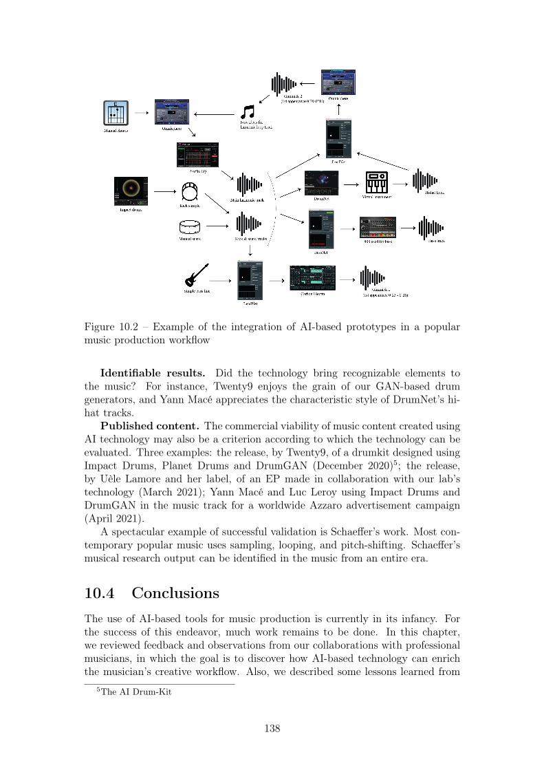
Figure 10.2 – Example of the integration of AI-based prototypes in a popularmusic production workflow

Identifiable results. Did the technology bring recognizable elements tothe music? For instance, Twenty9 enjoys the grain of our GAN-based drumgenerators, and Yann Macé appreciates the characteristic style of DrumNet’s hi-hat tracks.

Published content. The commercial viability of music content created usingAI technology may also be a criterion according to which the technology can beevaluated. Three examples: the release, by Twenty9, of a drumkit designed usingImpact Drums, Planet Drums and DrumGAN (December 2020)5; the release,by Uèle Lamore and her label, of an EP made in collaboration with our lab’stechnology (March 2021); Yann Macé and Luc Leroy using Impact Drums andDrumGAN in the music track for a worldwide Azzaro advertisement campaign(April 2021).

A spectacular example of successful validation is Schaeffer’s work. Most con-temporary popular music uses sampling, looping, and pitch-shifting. Schaeffer’smusical research output can be identified in the music from an entire era.

10.4 ConclusionsThe use of AI-based tools for music production is currently in its infancy. Forthe success of this endeavor, much work remains to be done. In this chapter,we reviewed feedback and observations from our collaborations with professionalmusicians, in which the goal is to discover how AI-based technology can enrichthe musician’s creative workflow. Also, we described some lessons learned from

5The AI Drum-Kit

138

this joint effort. In particular, for AI-based music innovation to work in practice,we believe it is essential to make user interaction an integral part of model designand development from the very start. Also, the characteristics that are relevantfor modeling vary widely from one musical style to another. This implies thatthe design of AI-based music technology cannot be style-agnostic. Lastly, wediscussed several ways of measuring the success of AI-based innovation in music.

Besides any technical limitations of AI, a present challenge for AI-based musicinnovation is a discrepancy between the expectations and perspectives of musi-cians on the one hand and engineers on the other. We believe that over timethese discrepancies will diminish and converge on the commodification of AI-based technology. It is conceivable that in the future, musicians will have anarsenal of AI techniques at their disposal, training and tweaking machine learn-ing models as part of their creative process as easily as they use any other audiosoftware today.

139

140

Chapter 11

General Conclusion

The dream of machines recreating and responding to complex human behaviorpromises to radically transform how we produce music. As seen in Chapter 3,the advent of Deep Learning into the realm of music technology innovation maypave the way towards such a paradigm shift. This dissertation has studied Gen-erative Adversarial Networks (GANs), a specific deep learning technique, for thecontrollable and intuitive audio synthesis of musical sounds.

The use of GANs —and Deep Learning in general— for musical audio gen-eration is still in its infancy. Among the existing challenges in modeling musicalaudio [Dieleman et al., 2018], one that is fundamental is that of choosing thebest audio representation. We have seen in Chapter 2 that this may depend onthe specific type of acoustic source to be modeled (e.g., tonal, percussive) as wellas the neural network architecture (e.g., CNN, RNN). The choice of represen-tation may greatly influence how efficiently the neural network learns from theaudio data and the generation time. Therefore, in our first work, presented inChapter 5, we compared various common audio representations, including theraw audio waveform and several time-frequency representations, on the task ofaudio synthesis of tonal instrument sounds [Nistal et al., 2021c]. This work pro-vided some insights on the performance of these representations on a specificbenchmark convolutional Progressive Growing GAN [Karras et al., 2017]. Re-sults showed that the magnitude and Instantaneous Frequency (IF) of the STFTand the complex-valued STFT obtained the best quantitative metrics amongstall the compared representations.

Another essential aspect that we tackled in this thesis is that of conditioningthe GAN in order to learn controls over the generation process. We explored var-ious sources of conditional information for different means of control. Followingour first work, in Chapter 6, we presented DrumGAN [Nistal et al., 2020], an ad-versarial synthesizer of percussive sounds that can be controlled based on percep-tual features describing timbral properties (e.g., boominess, roughness, hardness).DrumGAN operates on complex-valued STFT audio data, which we observed toperform better than other representations on percussive sounds. As a result ofthis work, we scaled DrumGAN and built a commercially viable plug-in compat-ible with any Digital Audio Workstation (DAW) that generates high-definitiondrum sounds (i.e., 44.1 kHz sample-rate). Additionally, we learned an encoderthat enabled the re-synthesis of preexisting drum samples to generate variationsand, also, we added continuous control over the instrument classes (kick, snare,

141

and cymbals). Further described in Chapter 10, the success of DrumGAN wasembodied in the release of musical content by professional musicians affiliatedwith Sony ATV.

While DrumGAN demonstrated that given some preexisting conditional in-formation, we could induce in the GAN some control over high-level features ofsound, in most cases, we do not have access to such information, either becausedatasets lack the desired annotations or because we simply do not know how toextract a specific feature. Our third experiment, presented in Chapter 7, showsthat a pre-trained discriminative teacher model can be used to generate such la-bels. This work explored the use of Knowledge Distillation (KD) [Hinton et al.,2015], a framework for transferring knowledge from a teacher to a student neu-ral network, as a means to learn semantically intuitive controls in a GAN-drivensynthesizer of tonal sounds [Nistal et al., 2021b]. The teacher model [Kong et al.,2020b], pre-trained on the Audio Set data [Gemmeke et al., 2017], was used togenerate soft labels on the NSynth [Engel et al., 2017] dataset for 128 soundevent categories (e.g., sonar, singing-bowl, mantra, bicycle-bell, etc). Then, aGAN synthesizer was trained using such soft labels as conditional information.An interesting outcome of KD is that the student model can learn abstract rep-resentations of classes that are not explicitly represented in the training data butare somehow sparsely encoded on the aggregate [Hinton et al., 2015]. For exam-ple, the NSynth dataset does not contain any sonar sound, yet, a sonar soundmay be extrapolated from other sounds in the dataset. Learning such unrepre-sented classes is possible thanks to the additional information that exists in therelative probabilities of the soft labels —compared to hard, one-hot labels. Suchadditional information was coined Dark Knowledge [Hinton et al., 2014]; hencewe called our model DarkGAN. Results confirmed that DarkGAN could learnsome degree of control over attributes not directly represented in the trainingdata.

Most initial works on audio synthesis with GANs inherit the architecturefrom the computer vision literature, limiting the generation to fixed-duration au-dio in analogy to the fixed-sized image data [Donahue et al., 2019, Engel et al.,2019]. While this may be a natural choice in images, we are generally inter-ested in synthesizing audio of any duration when modeling sound, particularlyfor musical purposes. Along this line, in Chapter 8, we proposed a frameworkfor conditioning a GAN synthesizer on a sequence of discrete features capturingstep-wise time-dependent information, as well as on static features (a randomnoise vector and the pitch class) that ensured the global consistency of the gen-erated sound [Nistal et al., 2021a]. Such sequential features were learned usinga self-supervised learning technique called Vector-Quantized Contrastive Predic-tive Coding (VQCPC) [Hadjeres and Crestel, 2020], hence, we called our modelVQCPC-GAN. Compared to other forms of unsupervised representation learn-ing, a valuable characteristic of CPC is that one can choose to some extent whatinformation is captured in the learned codes. This is done by carefully designinga negative sampling strategy for the contrastive objective. In VQCPC-GAN, wedesigned the negative sampling in an intra-sequence fashion, forcing the learnedcodes to neglect any global aspects of the data (e.g., the pitch and instrumentclass). While baselines trained following the fixed-duration scheme scored best,results showed that VQCPC-GAN achieved comparable performance even when

142

generating variable-length audio. Also, we observed that the codes affected onlythe envelope of the generated audio and, indeed, did not exert any control overglobal aspects.

As we saw in Chapter 3, generative models can be conditioned on preex-isting audio content, generally, as means to provide dense information to thenetwork for, e.g., spectrogram inversion [Kumar et al., 2019] or audio enhance-ment [Michelsanti and Tan, 2017]. The vision of this thesis is to, one day, devisetools that can respond to rather complex musical dependencies, for example, inthe form of some preexisting sparse, musical audio context, e.g., the generation ofa bass-line given some recorded drums. Learning such intricate musical relation-ships between conditional-generated music audio pairs is complicated and wouldrequire large amounts of data. With this in mind, in Chapter 9, we designed apretext audio enhancement task tailored at learning such kinds of dependenciesin the future. Concretely, we proposed a GAN to restore heavily compressed MP3music to its uncompressed, high-quality form [Lattner and Nistal, 2021]. Resultsshowed that the GAN could improve the quality of the audio signals over theMP3 versions for high compression rates (i.e., 16 kbps, 32 kbps). Also, we notedthat a stochastic generator could generate outputs closer to the original signalsthan those generated by a deterministic generator.

As a direct consequence of the application of Artificial Intelligence to musicalproduction tasks, it is crucial to assess these novel technologies by bringing theartist in the loop. We believe that AI-driven music research should be carriedout as an interdisciplinary effort involving researchers and artists to effectivelydesign tools that can help enhance the music production experience by speedingworkflows and inspiring the creative process. This perspective is plotted in ourfinal work, presented in Chapter 10, where we reported on collaborations withprofessional artists, looking at how various in-house AI tools were used in practiceto produce music. We identified usage patterns, issues and challenges that arosefrom the practical use of these tools. Based on this, some recommendations andvalidation criteria were formulated to develop AI technology for contemporarypopular music.

11.1 Future WorkFollowing, we enumerate some interesting directions for future work:

• Modelling new acoustic sources. An obvious direction for extending ourresearch on adversarial audio synthesis is to broaden the variety of acous-tic sources in the training dataset. In this work, we have mainly focusedon modeling tonal instruments (see Chapters 5, 7, and 8) and percussivesounds (see Chapter 6). We also used in Chapter 9 music mixtures forrestoring heavily compressed MP3 music. An interesting endeavour for fu-ture research would be to consider other types of sound sources such asenvironmental sounds, sound effects, and other natural sound sources. Themain challenge is the availability of large datasets with such types of soundsas well as the design of efficient architectures with enough computationalcapacity to model all of these sound sources.

• Modeling polyphonic sources. In this project we have mainly focused

143

on modeling one-shot, monophonic sound sources. Another way to increasethe amount of training data and learn richer dependencies between instru-ment sources would be to train the model on multiple instruments playingsimultaneously (polyphonic and multitimbral). Adequate architectures anddata representations need to be found which allow for an efficient and cost-effective implementation of such methods. In order to achieve that goal,it is probably necessary for the model to attend to the different sourcesseparately (or perform any implicit or explicit way of source separation).

• Extending intuitive controls on neural audio synthesizers. In thisthesis, we studied various methods for learning controls in a neural network.As part of the prototype development for the continuation of this project,we will further investigate novel sources of conditional information (Attack,Decay, Sustain, and Release curves, MIDI, MEL, Principal Components,Captions), as well as unsupervised learning of factors of variation [Peebleset al., 2020, Karras et al., 2018]. Another possible direction for research is todesign distance measures or trajectory strategies for traversing latent spacesin a meaningful way or reducing their dimensionality for visualization andnavigation purposes.

• Investigating other audio representations. While we have comparedsome important and common audio representations, many other forms ofstructuring audio information exist that could help train lighter models thatcan learn more efficiently from the audio data (e.g., wavelet transforms [Luoet al., 2017], Differentiable Digital Signal Processing [Engel et al., 2020]).

• Reducing model size. Reducing models’ size and computational require-ments becomes crucial when deploying DL models on edge hardware or inmemory-limited settings (e.g., personal computer, a microprocessor). Thisproject aimed to develop DL-driven audio synthesis tools that musicianscan use as a VST plugin on their personal computers. Hence, a require-ment for our models is that they can run in —or close to— real-time ina CPU. Various methods for model compression exist that are worthy ofstudy: distillation [Hinton et al., 2015], pruning [Zhu and Gupta, 2018], lot-tery ticket hypothesis [Kalibhat et al., 2021], quantization [Gholami et al.,2021], and more.

• Adversarial Autoencoders. As opposed to plain GANs [Goodfellowet al., 2014], we saw that VAEs [Kingma and Welling, 2014] feature thepossibility to encode data back into points in the latent space using an en-coder. However, VAEs have the added difficulty of imposing the specificdataset through a reconstruction loss (i.e., explicit density estimation) and,due to the variational encoding, they are known to produce blurry outputs.Following existing research, one interesting avenue for research is Gener-ative Adversarial Autoencoders [Pidhorskyi et al., 2020]. This frameworkwas shown in computer vision to join the data quality and sharpness of theGANs with the autoencoding capabilities of VAEs.

• Hierarchical VQCPC: VQCPC-GAN [Nistal et al., 2021a] proposed touse a sequence of tokens extracted from real audio data as conditional input

144

to a GAN architecture. In this work, a token corresponded to a cluster oftime-frequency frames (i.e., one token per frame). A promising researchline, inspired by previous work [Dhariwal et al., 2020], is to use a hierarchyof VQCPC encoders, where tokens produced by higher VQCPC encodersin the hierarchy account for longer-term segments of audio (i.e., more thanone frame) in order to learn features capturing structure at broader scales.By conditioning the GAN on both fine-grain and long-term tokens of thesequential data, we hope to control the structure of the generated data atvarious time scales.

145

Appendices

146

A. Figure Acknowledgements• Computer Music Icon from pngrepo.com

• Musicians Icon from Free Icons Library

• Hand icon by technology from shareicon.net

• Icon synth made by Hum from NounProject.com

• Sound Waves icon by Alice Noir from NounProject.com

• Hearing by Marek Polakovic from NounProject.com

• Idea Icon by Memed Nurrohmad from NounProject.com

• Extrasensory Perception by Andrew Forrester from NounProject.com

• Rock N Roll by Daouna Jeong from NounProject.com

• Fist by Cesar Reynoso from NounProject.com

• Note by Aleksandr Vector from NounProject.com

• Heart by Unicons Font from NounProject.com

• Customer Satisfaction by Luis Prado from NounProject.com

• Faders by Ashley van Dyck from NounProject.com

147

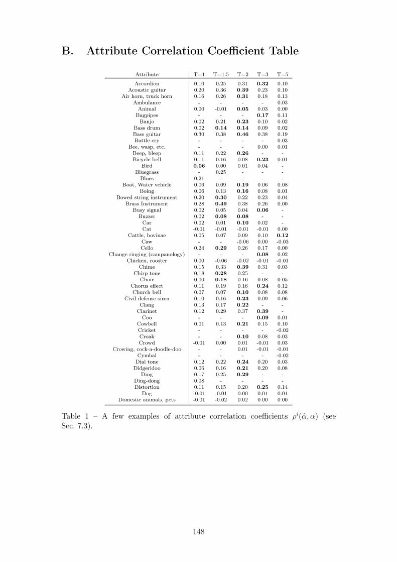
B. Attribute Correlation Coefficient Table

Attribute T=1 T=1.5 T=2 T=3 T=5

Accordion 0.10 0.25 0.31 0.32 0.10Acoustic guitar 0.20 0.36 0.39 0.23 0.10

Air horn, truck horn 0.16 0.26 0.31 0.18 0.13Ambulance - - - - 0.03Animal 0.00 -0.01 0.05 0.03 0.00Bagpipes - - - 0.17 0.11Banjo 0.02 0.21 0.23 0.10 0.02

Bass drum 0.02 0.14 0.14 0.09 0.02Bass guitar 0.30 0.38 0.46 0.38 0.19Battle cry - - - - 0.03

Bee, wasp, etc. - - - 0.00 0.01Beep, bleep 0.11 0.22 0.26 - -Bicycle bell 0.11 0.16 0.08 0.23 0.01

Bird 0.06 0.00 0.01 0.04 -Bluegrass - 0.25 - - -Blues 0.21 - - - -

Boat, Water vehicle 0.06 0.09 0.19 0.06 0.08Boing 0.06 0.13 0.16 0.08 0.01

Bowed string instrument 0.20 0.30 0.22 0.23 0.04Brass Instrument 0.28 0.49 0.38 0.26 0.00

Busy signal 0.02 0.05 0.04 0.06 -Buzzer 0.02 0.08 0.08 - -Car 0.02 0.01 0.10 0.02 -Cat -0.01 -0.01 -0.01 -0.01 0.00

Cattle, bovinae 0.05 0.07 0.09 0.10 0.12Caw - - -0.06 0.00 -0.03Cello 0.24 0.29 0.26 0.17 0.00

Change ringing (campanology) - - - 0.08 0.02Chicken, rooster 0.00 -0.06 -0.02 -0.01 -0.01

Chime 0.15 0.33 0.39 0.31 0.03Chirp tone 0.18 0.28 0.25 - -

Choir 0.00 0.18 0.16 0.08 0.05Chorus effect 0.11 0.19 0.16 0.24 0.12Church bell 0.07 0.07 0.10 0.08 0.08

Civil defense siren 0.10 0.16 0.23 0.09 0.06Clang 0.13 0.17 0.22 - -

Clarinet 0.12 0.29 0.37 0.39 -Coo - - - 0.09 0.01

Cowbell 0.01 0.13 0.21 0.15 0.10Cricket - - - - -0.02Croak - - 0.10 0.08 0.03Crowd -0.01 0.00 0.01 -0.01 0.03

Crowing, cock-a-doodle-doo - - 0.01 -0.01 -0.01Cymbal - - - - -0.02Dial tone 0.12 0.22 0.24 0.20 0.03Didgeridoo 0.06 0.16 0.21 0.20 0.08

Ding 0.17 0.25 0.29 - -Ding-dong 0.08 - - - -Distortion 0.11 0.15 0.20 0.25 0.14

Dog -0.01 -0.01 0.00 0.01 0.01Domestic animals, pets -0.01 -0.02 0.02 0.00 0.00

Table 1 – A few examples of attribute correlation coefficients ρi(α, α) (seeSec. 7.3).

148

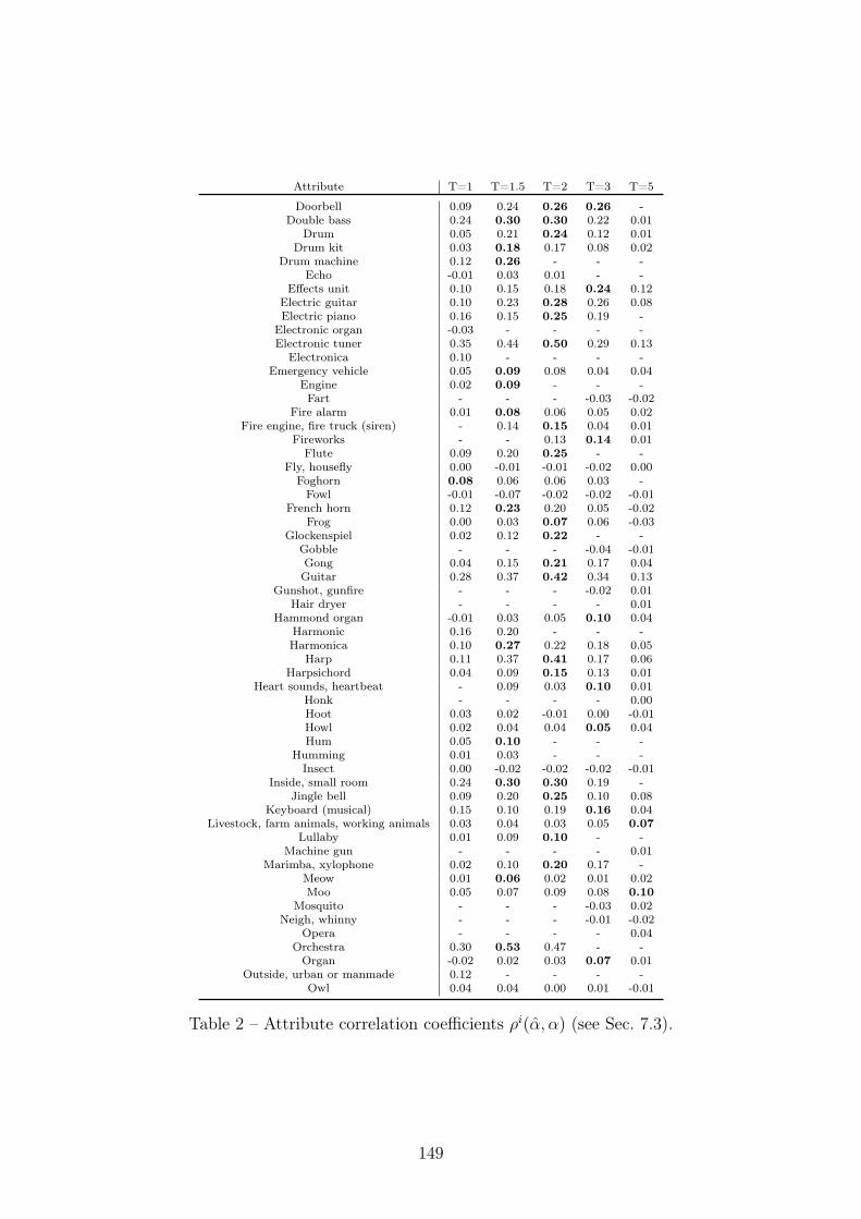
Attribute T=1 T=1.5 T=2 T=3 T=5

Doorbell 0.09 0.24 0.26 0.26 -Double bass 0.24 0.30 0.30 0.22 0.01

Drum 0.05 0.21 0.24 0.12 0.01Drum kit 0.03 0.18 0.17 0.08 0.02

Drum machine 0.12 0.26 - - -Echo -0.01 0.03 0.01 - -

Effects unit 0.10 0.15 0.18 0.24 0.12Electric guitar 0.10 0.23 0.28 0.26 0.08Electric piano 0.16 0.15 0.25 0.19 -

Electronic organ -0.03 - - - -Electronic tuner 0.35 0.44 0.50 0.29 0.13

Electronica 0.10 - - - -Emergency vehicle 0.05 0.09 0.08 0.04 0.04

Engine 0.02 0.09 - - -Fart - - - -0.03 -0.02

Fire alarm 0.01 0.08 0.06 0.05 0.02Fire engine, fire truck (siren) - 0.14 0.15 0.04 0.01

Fireworks - - 0.13 0.14 0.01Flute 0.09 0.20 0.25 - -

Fly, housefly 0.00 -0.01 -0.01 -0.02 0.00Foghorn 0.08 0.06 0.06 0.03 -Fowl -0.01 -0.07 -0.02 -0.02 -0.01

French horn 0.12 0.23 0.20 0.05 -0.02Frog 0.00 0.03 0.07 0.06 -0.03

Glockenspiel 0.02 0.12 0.22 - -Gobble - - - -0.04 -0.01Gong 0.04 0.15 0.21 0.17 0.04Guitar 0.28 0.37 0.42 0.34 0.13

Gunshot, gunfire - - - -0.02 0.01Hair dryer - - - - 0.01

Hammond organ -0.01 0.03 0.05 0.10 0.04Harmonic 0.16 0.20 - - -Harmonica 0.10 0.27 0.22 0.18 0.05

Harp 0.11 0.37 0.41 0.17 0.06Harpsichord 0.04 0.09 0.15 0.13 0.01

Heart sounds, heartbeat - 0.09 0.03 0.10 0.01Honk - - - - 0.00Hoot 0.03 0.02 -0.01 0.00 -0.01Howl 0.02 0.04 0.04 0.05 0.04Hum 0.05 0.10 - - -

Humming 0.01 0.03 - - -Insect 0.00 -0.02 -0.02 -0.02 -0.01

Inside, small room 0.24 0.30 0.30 0.19 -Jingle bell 0.09 0.20 0.25 0.10 0.08

Keyboard (musical) 0.15 0.10 0.19 0.16 0.04Livestock, farm animals, working animals 0.03 0.04 0.03 0.05 0.07

Lullaby 0.01 0.09 0.10 - -Machine gun - - - - 0.01

Marimba, xylophone 0.02 0.10 0.20 0.17 -Meow 0.01 0.06 0.02 0.01 0.02Moo 0.05 0.07 0.09 0.08 0.10

Mosquito - - - -0.03 0.02Neigh, whinny - - - -0.01 -0.02

Opera - - - - 0.04Orchestra 0.30 0.53 0.47 - -Organ -0.02 0.02 0.03 0.07 0.01

Outside, urban or manmade 0.12 - - - -Owl 0.04 0.04 0.00 0.01 -0.01

Table 2 – Attribute correlation coefficients ρi(α, α) (see Sec. 7.3).

149

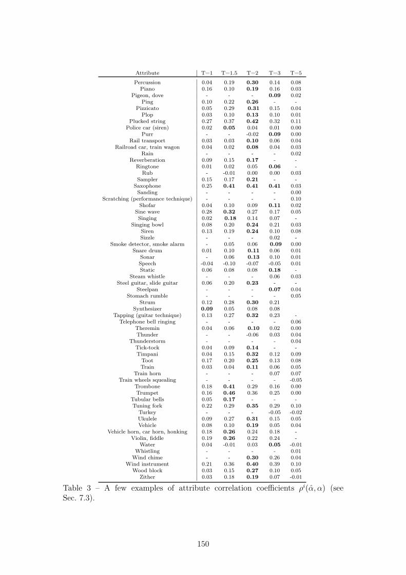
Attribute T=1 T=1.5 T=2 T=3 T=5

Percussion 0.04 0.19 0.30 0.14 0.08Piano 0.16 0.10 0.19 0.16 0.03

Pigeon, dove - - - 0.09 0.02Ping 0.10 0.22 0.26 - -

Pizzicato 0.05 0.29 0.31 0.15 0.04Plop 0.03 0.10 0.13 0.10 0.01

Plucked string 0.27 0.37 0.42 0.32 0.11Police car (siren) 0.02 0.05 0.04 0.01 0.00

Purr - - -0.02 0.09 0.00Rail transport 0.03 0.03 0.10 0.06 0.04

Railroad car, train wagon 0.04 0.02 0.08 0.04 0.03Rain - - - - 0.02

Reverberation 0.09 0.15 0.17 - -Ringtone 0.01 0.02 0.05 0.06 -

Rub - -0.01 0.00 0.00 0.03Sampler 0.15 0.17 0.21 - -

Saxophone 0.25 0.41 0.41 0.41 0.03Sanding - - - - 0.00

Scratching (performance technique) - - - - 0.10Shofar 0.04 0.10 0.09 0.11 0.02

Sine wave 0.28 0.32 0.27 0.17 0.05Singing 0.02 0.18 0.14 0.07 -

Singing bowl 0.08 0.20 0.24 0.21 0.03Siren 0.13 0.19 0.24 0.10 0.08Sizzle - - - 0.02 -

Smoke detector, smoke alarm - 0.05 0.06 0.09 0.00Snare drum 0.01 0.10 0.11 0.06 0.01

Sonar - 0.06 0.13 0.10 0.01Speech -0.04 -0.10 -0.07 -0.05 0.01Static 0.06 0.08 0.08 0.18 -

Steam whistle - - - 0.06 0.03Steel guitar, slide guitar 0.06 0.20 0.23 - -

Steelpan - - - 0.07 0.04Stomach rumble - - - - 0.05

Strum 0.12 0.28 0.30 0.21Synthesizer 0.09 0.05 0.08 0.08

Tapping (guitar technique) 0.13 0.27 0.32 0.23 -Telephone bell ringing - - - - 0.06

Theremin 0.04 0.06 0.10 0.02 0.00Thunder - - -0.06 0.03 0.04

Thunderstorm - - - - 0.04Tick-tock 0.04 0.09 0.14 - -Timpani 0.04 0.15 0.32 0.12 0.09Toot 0.17 0.20 0.25 0.13 0.08Train 0.03 0.04 0.11 0.06 0.05

Train horn - - - 0.07 0.07Train wheels squealing - - - - -0.05

Trombone 0.18 0.41 0.29 0.16 0.00Trumpet 0.16 0.46 0.36 0.25 0.00

Tubular bells 0.05 0.17 - - -Tuning fork 0.22 0.29 0.35 0.29 0.10

Turkey - - - -0.05 -0.02Ukulele 0.09 0.27 0.31 0.15 0.05Vehicle 0.08 0.10 0.19 0.05 0.04

Vehicle horn, car horn, honking 0.18 0.26 0.24 0.18 -Violin, fiddle 0.19 0.26 0.22 0.24 -

Water 0.04 -0.01 0.03 0.05 -0.01Whistling - - - - 0.01

Wind chime - - 0.30 0.26 0.04Wind instrument 0.21 0.36 0.40 0.39 0.10

Wood block 0.03 0.15 0.27 0.10 0.05Zither 0.03 0.18 0.19 0.07 -0.01

Table 3 – A few examples of attribute correlation coefficients ρi(α, α) (seeSec. 7.3).

150

Bibliography

Y. Ai, H.-C. Wu, and Z.-H. Ling. SampleRNN-Based Neural Vocoderfor Statistical Parametric Speech Synthesis. page 91, 2018. URLhttp://mirlab.org/conference_papers/International_Conference/ICASSP2018/pdfs/0005659.pdf.

R. Anil, G. Pereyra, A. Passos, R. Ormándi, G. E. Dahl, and G. E. Hinton.Large scale distributed neural network training through online distillation. In6th International Conference on Learning Representations, ICLR, Vancouver,BC, Canada, May 2018.

C. Aouameur, P. Esling, and G. Hadjeres. Neural drum machine: An interactivesystem for real-time synthesis of drum sounds. In Proc. of the 10th InternationalConference on Computational Creativity, ICCC, Charlotte, North Carolina,USA, June 2019.

M. Aramaki, R. Kronland-Martinet, T. Voinier, and S. Ystad. A percussive soundsynthesizer based on physical and perceptual attributes. Comput. Music. J.,30(2):32–41, 2006. doi: 10.1162/comj.2006.30.2.32. URL https://doi.org/10.1162/comj.2006.30.2.32.

M. Aramaki, M. Besson, R. Kronland-Martinet, and S. Ystad. Controlling thePerceived Material in an Impact Sound Synthesizer. IEEE Trans. Speech AudioProcess., 19(2):301–314, 2011a. doi: 10.1109/TASL.2010.2047755. URL https://doi.org/10.1109/TASL.2010.2047755.

M. Aramaki, R. Kronland-Martinet, and S. Ystad. Perceptual control of environ-mental sound synthesis. In Speech, Sound and Music Processing: EmbracingResearch in India - 8th International Symposium, CMMR, 20th InternationalSymposium, FRSM, volume 7172 of Lecture Notes in Computer Science, pages172–186, Bhubaneswar, India, March 2011b. Springer.

S. Ö. Arik, M. Chrzanowski, A. Coates, G. F. Diamos, A. Gibiansky, Y. Kang,X. Li, J. Miller, A. Y. Ng, J. Raiman, S. Sengupta, and M. Shoeybi. DeepVoice: Real-time Neural Text-to-Speech. In Proceedings of the 34th Interna-tional Conference on Machine Learning, ICML, pages 195–204, Sydney, NSW,Australia, August 2017.

M. Arjovsky, S. Chintala, and L. Bottou. Wasserstein GAN. CoRR,abs/1701.07875, 2017.

T. Asami, R. Masumura, Y. Yamaguchi, H. Masataki, and Y. Aono. Domainadaptation of DNN acoustic models using knowledge distillation. In IEEE

151

International Conference on Acoustics, Speech and Signal Processing, ICASSP,pages 5185–5189, New Orleans, LA, USA, March 2017. IEEE. doi: 10.1109/ICASSP.2017.7953145.

Y. Aytar, C. Vondrick, and A. Torralba. SoundNet: Learning Sound Repre-sentations from Unlabeled Video. In Annual Conference on Neural Informa-tion Processing Systems, NeurIPS, pages 892–900, Barcelona, Spain, December2016.

J. Ba and R. Caruana. Do Deep Nets Really Need to be Deep? In Z. Ghahramani,M. Welling, C. Cortes, N. D. Lawrence, and K. Q. Weinberger, editors, An-nual Conference on Neural Information Processing Systems, pages 2654–2662,Montreal, Quebec, Canada, December 2014.

A. Baevski, S. Schneider, and M. Auli. vq-wav2vec: Self-Supervised Learning ofDiscrete Speech Representations. In ICLR, Addis Ababa, Ethiopia, Apr. 2020.

D. Bansal, B. Raj, and P. Smaragdis. Bandwidth expansion of narrowbandspeech using non-negative matrix factorization. In 9th European Conferenceon Speech Communication and Technology, INTERSPEECH, pages 1505–1508,Lisbon, Portugal, September 2005. ISCA. URL http://www.isca-speech.org/archive/interspeech_2005/i05_1505.html.

A. Barahona-Ríos and T. Collins. SpecSinGAN: Sound Effect Variation SynthesisUsing Single-Image GANs. CoRR, abs/2110.07311, 2021.

S. T. Barratt and R. Sharma. A Note on the Inception Score. CoRR,abs/1801.01973, 2018. URL http://arxiv.org/abs/1801.01973.

S. Barry and Y. Kim. “Style” Transfer for Musical Audio Using Multiple Time-Frequency Representations, 2018. URL https://openreview.net/forum?id=BybQ7zWCb.

T. Bazin, G. Hadjeres, P. Esling, and M. Malt. Spectrogram Inpainting forInteractive Generation of Instrument Sounds. In Joint Conference on AI MusicCreativity, 2020.

S. Bengio, O. Vinyals, N. Jaitly, and N. Shazeer. Scheduled Sampling for SequencePrediction with Recurrent Neural Networks. In Advances in Neural InformationProcessing Systems 28: Annual Conference on Neural Information ProcessingSystems NeurIPS.

Y. Bengio, A. C. Courville, and P. Vincent. Representation Learning: A Reviewand New Perspectives. IEEE Trans. Pattern Anal. Mach. Intell., 35(8), 2013.

M. Binkowski, D. J. Sutherland, M. Arbel, and A. Gretton. Demystifying MMDgans. In ICLR, Vancouver, BC, Canada, Apr. 2018.

M. Binkowski, J. Donahue, S. Dieleman, A. Clark, E. Elsen, N. Casagrande,L. C. Cobo, and K. Simonyan. High Fidelity Speech Synthesis with AdversarialNetworks. In 8th International Conference on Learning Representations, ICLR,Addis Ababa, Ethiopia, April 2020.

152

A. Biswas and D. Jia. Audio Codec Enhancement with Generative AdversarialNetworks. In 2020 IEEE International Conference on Acoustics, Speech andSignal Processing, ICASSP, pages 356–360, Barcelona, Spain, May 2020. IEEE.doi: 10.1109/ICASSP40776.2020.9053113.

A. Bitton, P. Esling, A. Caillon, and M. Fouilleul. Assisted Sound SampleGeneration with Musical Conditioning in Adversarial Auto-Encoders. CoRR,abs/1904.06215, 2019.

A. Bitton, P. Esling, and T. Harada. Neural Granular Sound Synthesis. CoRR,abs/2008.01393, 2020.

M. Blaauw and J. Bonada. Modeling and Transforming Speech Using VariationalAutoencoders. In 17th Annual Conference of the International Speech Commu-nication Association, INTERSPEECH, pages 1770–1774, San Francisco, CA,USA, September 2016. ISCA.

M. Blaauw and J. Bonada. A neural parametric singing synthesizer. In 18thAnnual Conference of the International Speech Communication Association,INTERSPEECH, pages 4001–4005, Stockholm, Sweden, August 2017.

B. Boashash. Estimating and interpreting the instantaneous frequency of a signal.II. Algorithms and applications. Proc. of the IEEE, 80(4):550–568, Apr. 1992.ISSN 1558-2256. doi: 10.1109/5.135378.

S. Boll. Suppression of acoustic noise in speech using spectral subtraction. IEEETransactions on Acoustics, Speech, and Signal Processing, 27(2):113–120, 1979.doi: 10.1109/TASSP.1979.1163209.

S. Bond-Taylor, A. Leach, Y. Long, and C. G. Willcocks. Deep Generative Mod-elling: A Comparative Review of VAEs, GANs, Normalizing Flows, Energy-Based and Autoregressive Models. CoRR, abs/2103.04922, 2021.

K. Brandenburg. MP3 and AAC explained. In Audio Engineering Society Con-ference: 17th International Conference: High-Quality Audio Coding. AudioEngineering Society, 1999.

K. Brandenburg and G. Stoll. Iso/mpeg-1 audio: A generic standard for codingof high-quality digital audio. Journal of the Audio Engineering Society, 42(10):780–792, 1994.

J. Briot, G. Hadjeres, and F. Pachet. Deep Learning Techniques for Music Gen-eration - A Survey. CoRR, abs/1709.01620, 2017. URL http://arxiv.org/abs/1709.01620.

A. Brock, J. Donahue, and K. Simonyan. Large Scale GAN Training for HighFidelity Natural Image Synthesis. In 7th International Conference on LearningRepresentations, ICLR, New Orleans, LA, USA, May 2019. OpenReview.net.

J. C. Brown. Calculation of a constant-Q spectral transform. Journal of theAcoustical Society of America, 89(1):425–434, 1991. ISSN 0001-4966. doi:10.1121/1.400476.

153

G. Brunner, A. Konrad, Y. Wang, and R. Wattenhofer. MIDI-VAE: ModelingDynamics and Instrumentation of Music with Applications to Style Transfer. InProceedings of the 19th International Society for Music Information RetrievalConference, ISMIR, 2018, pages 747–754, Paris, France, September 2018a.

G. Brunner, Y. Wang, R. Wattenhofer, and S. Zhao. Symbolic Music GenreTransfer with CycleGAN. In IEEE 30th International Conference on Toolswith Artificial Intelligence, ICTAI, pages 786–793, Volos, Greece, November2018b.

C. Bucila, R. Caruana, and A. Niculescu-Mizil. Model compression. In T. Eliassi-Rad, L. H. Ungar, M. Craven, and D. Gunopulos, editors, Proceedings of theTwelfth ACM SIGKDD International Conference on Knowledge Discovery andData Mining, pages 535–541, Philadelphia, PA, USA, August 2006. ACM.

H. Caesar, J. R. R. Uijlings, and V. Ferrari. COCO-Stuff: Thing and StuffClasses in Context. In 2018 IEEE Conference on Computer Vision and PatternRecognition, CVPR, pages 1209–1218, Salt Lake City, UT, USA, June 2018.IEEE Computer Society. doi: 10.1109/CVPR.2018.00132.

A. Camurri, S. Hashimoto, M. Ricchetti, A. Ricci, K. Suzuki, R. Trocca, andG. Volpe. EyesWeb: Toward Gesture and Affect Recognition in InteractiveDance and Music Systems. Comput. Music. J., 24(1):57–69, 2000.

H. Caracalla and A. Roebel. Sound Texture Synthesis Using RI Spectrograms.In 2020 IEEE International Conference on Acoustics, Speech and Signal Pro-cessing, ICASSP, 2020, pages 416–420, Barcelona, Spain, May 2020. IEEE.

W. Chan, N. R. Ke, and I. Lane. Transferring knowledge from a RNN to a DNN.In 16th Annual Conference of the International Speech Communication Associ-ation, INTERSPEECH, pages 3264–3268, Dresden, Germany, September 2015.ISCA.

F. Chen, R. Huang, C. Cui, Y. Ren, J. Liu, Z. Zhao, N. Yuan, and B. Huai.SingGAN: Generative Adversarial Network For High-Fidelity Singing VoiceGeneration. 2021.

J. Chen, Y. Wang, S. Yoho, D. Wang, and E. Healy. Large-scale training toincrease speech intelligibility for hearing-impaired listeners in novel noises. TheJournal of the Acoustical Society of America, 139:2604–2612, 05 2016a. doi:10.1121/1.4948445.

L. Chen, S. Srivastava, Z. Duan, and C. Xu. Deep Cross-Modal Audio-VisualGeneration. In Proceedings of the on Thematic Workshops of ACM Multimedia,pages 349–357, Mountain View, CA, USA, October 2017.

T. Chen, S. Kornblith, M. Norouzi, and G. Hinton. A simple framework forcontrastive learning of visual representations. In International conference onmachine learning, pages 1597–1607. PMLR, 2020.

154

X. Chen, Y. Duan, R. Houthooft, J. Schulman, I. Sutskever, and P. Abbeel.InfoGAN: Interpretable Representation Learning by Information MaximizingGenerative Adversarial Nets. In Advances in Neural Information ProcessingSystems 29: Annual Conference on Neural Information Processing Systems,NeurIPS, pages 2172–2180, Barcelona, Spain, December 2016b.

R. Child, S. Gray, A. Radford, and I. Sutskever. Generating Long Sequences withSparse Transformers. CoRR, abs/1904.10509, 2019.

Y. Choi, M. Choi, M. Kim, J. Ha, S. Kim, and J. Choo. StarGAN: Unified Gener-ative Adversarial Networks for Multi-Domain Image-to-Image Translation. InIEEE Conference on Computer Vision and Pattern Recognition, CVPR, pages8789–8797, Salt Lake City, UT, USA, June 2018.

J. Chorowski, R. J. Weiss, S. Bengio, and A. van den Oord. Unsupervised speechrepresentation learning using wavenet autoencoders. CoRR, abs/1901.08810,2019. URL http://arxiv.org/abs/1901.08810.

J. M. Chowning. The synthesis of complex audio spectra by means of frequencymodulation. Journal of the Audio Engineering Society, 21(7):526–534, Septem-ber 1973.

O. Cífka, A. Ozerov, U. Simsekli, and G. Richard. Self-Supervised VQ-VAE ForOne-Shot Music Style Transfer. CoRR, abs/2102.05749, 2021.

Clark E. et al. Creative writing with a machine in the loop: Case studies onslogans and stories. In IUI, pages 329–340. ACM, March 2018. doi: 10.1145/3172944.3172983. URL https://doi.org/10.1145/3172944.3172983.

M. Comunità, H. Phan, and J. D. Reiss. Neural synthesis of footsteps soundeffects with generative adversarial networks, 2021.

S. Conan. Intuitive Control of Solid-Interaction Sounds Synthesis: Toward SonicMetaphors. 2014.

S. Conan, E. Thoret, M. Aramaki, O. Derrien, C. Gondre, S. Ystad, andR. Kronland-Martinet. An Intuitive Synthesizer of Continuous-InteractionSounds: Rubbing, Scratching, and Rolling. Comput. Music. J., 38(4):24–37,2014. doi: 10.1162/COMJ\_a\_00266. URL https://doi.org/10.1162/COMJ_a_00266.

A. Cont. Musical Research at Ircam. Taylor & Francis, Apr 2013. doi: 10.1080/07494467.2013.774121. URL https://hal.inria.fr/hal-00930937.

I. Corbett. What data compression does to your music,2012. URL https://www.soundonsound.com/techniques/what-data-compression-does-your-music. Accessed 31 May 2021.

S. Crab. 120 Years Of Electronic Music - The history of electronic music from1800 to 2015, 2016. URL http://120years.net/https://120years.net/category/date/1800-1900/.

155

S. B. Davis and P. Mermelstein. Comparison of parametric representations formonosyllabic word recognition in continuously spoken sentences. IEEE Trans.Acoust. Speech, Signal Process., pages 357–366, 1980.

M. Dendrinos, S. Bakamidis, and G. Carayannis. Speech enhancement from noise:A regenerative approach. Speech Commun., 10(1):45–57, 1991. doi: 10.1016/0167-6393(91)90027-Q. URL https://doi.org/10.1016/0167-6393(91)90027-Q.

J. Deng, W. Dong, R. Socher, L.-J. Li, K. Li, and L. Fei-Fei. ImageNet: A Large-Scale Hierarchical Image Database. In IEEE Conference on Computer Visionand Pattern Recognition, CVPR, June 2009.

J. Deng, B. W. Schuller, F. Eyben, D. Schuller, Z. Zhang, H. Francois, andE. Oh. Exploiting time-frequency patterns with LSTM-RNNs for low-bitrateaudio restoration. Neural Comput. Appl., 32(4):1095–1107, 2020. doi: 10.1007/s00521-019-04158-0. URL https://doi.org/10.1007/s00521-019-04158-0.

E. L. Denton, S. Gross, and R. Fergus. Semi-Supervised Learning with Context-Conditional Generative Adversarial Networks. volume abs/1611.06430, 2016.

P. Dhariwal, H. Jun, C. Payne, J. W. Kim, A. Radford, and I. Sutskever. Jukebox:A generative model for music. CoRR, abs/2005.00341, 2020.

S. Dieleman. Generating Music in the Waveform Domain. https://benanne.github.io/2020/03/24/audio-generation.html, 2020.

S. Dieleman and B. Schrauwen. End-to-end learning for music audio. In ICASSP,pages 6964–6968, Florence, Italy, May 2014. doi: 10.1109/ICASSP.2014.6854950.

S. Dieleman, A. van den Oord, and K. Simonyan. The challenge of realisticmusic generation: modelling raw audio at scale. In NeurIPS, pages 8000–8010,Montréal, Canada, Dec. 2018.

M. Dietz, L. Liljeryd, K. Kjorling, and O. Kunz. Spectral Band Replication, anovel approach in audio coding. In Audio Engineering Society Convention 112.Audio Engineering Society, 2002.

C. Donahue, B. Li, and R. Prabhavalkar. Exploring Speech Enhancement withGenerative Adversarial Networks for Robust Speech Recognition. In IEEEInternational Conference on Acoustics, Speech and Signal Processing, ICASSP,pages 5024–5028, Calgary, AB, Canada, April 2018. IEEE.

C. Donahue, J. McAuley, and M. Puckette. Adversarial Audio Synthesis. In Proc.of the 7th International Conference on Learning Representations, ICLR, May2019.

C. Dong, C. C. Loy, K. He, and X. Tang. Image Super-Resolution Using DeepConvolutional Networks. IEEE Trans. Pattern Anal. Mach. Intell., 38(2):295–307, 2016. doi: 10.1109/TPAMI.2015.2439281. URL https://doi.org/10.1109/TPAMI.2015.2439281.

156

J. Dong, W. Wang, and J. A. Chambers. Audio super-resolution using anal-ysis dictionary learning. In 2015 IEEE International Conference on DigitalSignal Processing, DSP, pages 604–608, Singapore, July 2015. IEEE. doi:10.1109/ICDSP.2015.7251945. URL https://doi.org/10.1109/ICDSP.2015.7251945.

J. Drysdale, M. Tomczak, and J. Hockman. Adversarial Synthesis of DrumSounds. In DAFX, 2020.

J. Engel, C. Resnick, A. Roberts, S. Dieleman, M. Norouzi, D. Eck, and K. Si-monyan. Neural Audio Synthesis of Musical Notes with WaveNet Autoen-coders. In Proc. of the 34th International Conference on Machine Learning,ICML, Sydney, NSW, Australia, Aug. 2017.

J. Engel, K. K. Agrawal, S. Chen, I. Gulrajani, C. Donahue, and A. Roberts.GANSynth: Adversarial Neural Audio Synthesis. In Proc. of the 7th Interna-tional Conference on Learning Representations, ICLR, May 2019.

J. H. Engel, L. Hantrakul, C. Gu, and A. Roberts. DDSP: Differentiable DigitalSignal Processing. In Proc. of the 8th International Conference on LearningRepresentations, ICLR, Addis Ababa, Ethiopia, Apr. 2020.

Y. Ephraim. Statistical-model-based speech enhancement systems. Proceedingsof the IEEE, 80(10):1526–1555, 1992. doi: 10.1109/5.168664.

H. Erdogan, J. R. Hershey, S. Watanabe, and J. L. Roux. Phase-sensitive andrecognition-boosted speech separation using deep recurrent neural networks.In IEEE International Conference on Acoustics, Speech and Signal Processing,ICASSP, pages 708–712, South Brisbane, Queensland, Australia, April 2015.IEEE.

P. Esling, A. Chemla-Romeu-Santos, and A. Bitton. Bridging Audio Analy-sis, Perception and Synthesis with Perceptually-regularized Variational TimbreSpaces. In Proceedings of the 19th International Society for Music InformationRetrieval Conference, ISMIR, pages 175–181, Paris, France, September 2018a.

P. Esling, A. Chemla-Romeu-Santos, and A. Bitton. Generative timbre spaceswith variational audio synthesis. In Proc. of the 21st International Conferenceon Digital Audio Effects DAFx-18, Aveiro, Portugal, Sept. 2018b.

P. Esling, N. Masuda, A. Bardet, R. Despres, and A. Chemla-Romeu-Santos.Universal audio synthesizer control with normalizing flows. Journal of AppliedSciences, 2019.

C. Esteban, S. L. Hyland, and G. Rätsch. Real-valued (Medical) Time SeriesGeneration with Recurrent Conditional GANs. CoRR, 2017.

Y. Fan, Y. Qian, F. Xie, and F. K. Soong. TTS synthesis with bidirectionalLSTM based recurrent neural networks. In INTERSPEECH, Sept. 2014.

K. Fisher and A. Scherlis. WaveMedic: Convolutional Neural Networks for SpeechAudio Enhancement. 2016.

157

S. Fu, C. Liao, Y. Tsao, and S. Lin. MetricGAN: Generative Adversarial Net-works based Black-box Metric Scores Optimization for Speech Enhancement.In K. Chaudhuri and R. Salakhutdinov, editors, Proceedings of the 36th Inter-national Conference on Machine Learning, ICML, volume 97 of Proceedings ofMachine Learning Research, pages 2031–2041, Long Beach, California, USA,June 2019. PMLR.

J. Fuegi and J. Francis. Lovelace & Babbage and the creation of the 1843 ’notes’.Inroads, 6(3):78–86, 2015. doi: 10.1145/2810201. URL https://doi.org/10.1145/2810201.

L. Gao, K. Xu, H. Wang, and Y. Peng. Multi-Representation Knowledge Distil-lation For Audio Classification. CoRR, abs/2002.09607, 2020.

L. A. Gatys, A. S. Ecker, and M. Bethge. A neural algorithm of artistic style.arXiv preprint arXiv:1508.06576, 2015.

J. F. Gemmeke, D. P. W. Ellis, D. Freedman, A. Jansen, W. Lawrence, R. C.Moore, M. Plakal, and M. Ritter. Audio Set: An ontology and human-labeleddataset for audio events. In Proc. IEEE ICASSP 2017, New Orleans, LA, 2017.

F. G. Germain, Q. Chen, and V. Koltun. Speech Denoising with Deep FeatureLosses. In 20th Annual Conference of the International Speech Communica-tion Association, INTERSPEECH, pages 2723–2727, Graz, Austria, September2019. ISCA.

A. Gholami, S. Kim, Z. Dong, Z. Yao, M. W. Mahoney, and K. Keutzer. ASurvey of Quantization Methods for Efficient Neural Network Inference. CoRR,abs/2103.13630, 2021.

A. Gibiansky, S. Ö. Arik, G. F. Diamos, J. Miller, K. Peng, W. Ping, J. Raiman,and Y. Zhou. Deep Voice 2: Multi-Speaker Neural Text-to-Speech. In Advancesin Neural Information Processing Systems 30: Annual Conference on NeurIPS,pages 2966–2974, Long Beach, CA, USA, December 2017.

I. J. Goodfellow. NIPS 2016 Tutorial: Generative Adversarial Networks. CoRR,abs/1701.00160, 2017. URL http://arxiv.org/abs/1701.00160.

I. J. Goodfellow, J. Pouget-Abadie, M. Mirza, B. Xu, D. Warde-Farley, S. Ozair,A. C. Courville, and Y. Bengio. Generative Adversarial Nets. In NeurIPS,pages 2672–2680, Montreal, Quebec, Canada, Dec. 2014.

R. Gordon. Synthesizing Drums: The Bass Drum. Sound OnSound, Jan. 2002a. URL https://www.soundonsound.com/techniques/synthesizing-drums-bass-drum.

R. Gordon. Synthesizing drums: The snare drum. Sound OnSound, Jan. 2002b. URL https://www.soundonsound.com/techniques/synthesizing-drums-snare-drum.

M. Grachten, E. Deruty, and A. Tanguy. Auto-adaptive Resonance Equalizationusing Dilated Residual Networks. In Proceedings of the 20th ISMIR, Delft, The

158

Netherlands, 2019. URL http://archives.ismir.net/ismir2019/paper/000048.pdf.

M. Grachten, S. Lattner, and E. Deruty. BassNet: A Variational Gated Autoen-coder for Conditional Generation of Bass Guitar Tracks with Learned Interac-tive Control. Applied Sciences, 10(18), 2020. ISSN 2076-3417. doi: 10.3390/app10186627. URL https://www.mdpi.com/2076-3417/10/18/6627.

G. Greshler, T. R. Shaham, and T. Michaeli. Catch-A-Waveform: Learning toGenerate Audio from a Single Short Example. CoRR, abs/2106.06426, 2021.

A. Gretton, K. M. Borgwardt, M. J. Rasch, B. Schölkopf, and A. J. Smola. AKernel Two-Sample Test. J. of Mach. Learn. Res., 13:723–773, 2012.

D. W. Griffin and J. S. Lim. Signal estimation from modified short-time Fouriertransform. In ICASSP, pages 804–807, Boston, Massachusetts, USA, Apr. 1983.doi: 10.1109/ICASSP.1983.1172092.

I. Gulrajani, F. Ahmed, M. Arjovsky, V. Dumoulin, and A. C. Courville. Im-proved training of Wasserstein GANs. In NeurIPS, pages 5769–5779, LongBeach, CA, USA, Dec. 2017.

A. Gupta, B. Shillingford, Y. M. Assael, and T. C. Walters. Speech Band-width Extension with WaveNet. In IEEE Workshop on Applications of Sig-nal Processing to Audio and Acoustics, WASPAA, pages 205–208, New Paltz,NY, USA, October 2019. IEEE. doi: 10.1109/WASPAA.2019.8937169. URLhttps://doi.org/10.1109/WASPAA.2019.8937169.

C. Gupta, P. Kamath, and L. Wyse. Signal Representations for SynthesizingAudio Textures with Generative Adversarial Networks. CoRR, abs/2103.07390,2021.

G. Hadjeres and L. Crestel. Vector Quantized Contrastive Predictive Coding forTemplate-based Music Generation. CoRR, 2020.

G. Hadjeres, F. Pachet, and F. Nielsen. Deepbach: a steerable model for bachchorales generation. In Proceedings of the 34th International Conference onMachine Learning, ICML 2017, Sydney, NSW, Australia, 6-11 August 2017,pages 1362–1371, 2017.

K. He, X. Zhang, S. Ren, and J. Sun. Delving Deep into Rectifiers: SurpassingHuman-Level Performance on ImageNet Classification. In IEEE InternationalConference on Computer Vision, ICCV, Santiago, Chile, Dec. 2015.

O. J. Hénaff, A. Srinivas, J. D. Fauw, A. Razavi, C. Doersch, S. M. A. Eslami, andA. van den Oord. Data-Efficient Image Recognition with Contrastive PredictiveCoding. CoRR, abs/1905.09272, 2019.

G. Hinton, O. Vinyals, and J. Dean. Dark Knowledge. In Toyota TechnologicalInstitute at Chicago, TTIC, 2014.

G. E. Hinton, O. Vinyals, and J. Dean. Distilling the Knowledge in a NeuralNetwork. CoRR, abs/1503.02531, 2015.

159

E. Hosseini-Asl, Y. Zhou, C. Xiong, and R. Socher. A Multi-Discriminator Cy-cleGAN for Unsupervised Non-Parallel Speech Domain Adaptation. In Proc.of the 19th Annual Conference of the International Speech Communication As-sociation, Hyderabad, India, Sept. 2018.

W. Hsu, Y. Zhang, and J. R. Glass. Learning Latent Representations for SpeechGeneration and Transformation. In 18th Annual Conference of the Interna-tional Speech Communication Association, INTERSPEECH, pages 1273–1277,Stockholm, Sweden, August 2017.

Y. Hu, Y. Liu, S. Lv, M. Xing, S. Zhang, Y. Fu, J. Wu, B. Zhang, andL. Xie. DCCRN: Deep Complex Convolution Recurrent Network for Phase-Aware Speech Enhancement. In 21st Annual Conference of the Interna-tional Speech Communication Association, INTERSPEECH, pages 2472–2476,Shanghai, China, October 2020. ISCA. doi: 10.21437/Interspeech.2020-2537.URL https://doi.org/10.21437/Interspeech.2020-2537.

C. A. Huang, A. Vaswani, J. Uszkoreit, I. Simon, C. Hawthorne, N. Shazeer, A. M.Dai, M. D. Hoffman, M. Dinculescu, and D. Eck. Music Transformer: Gener-ating Music with Long-Term Structure. In ICLR (Poster). OpenReview.net,2019a.

C. A. Huang, H. V. Koops, E. Newton-Rex, M. Dinculescu, and C. J. Cai. AISong Contest: Human-AI Co-Creation in Songwriting. CoRR, abs/2010.05388,2020. URL https://arxiv.org/abs/2010.05388.

H. Huang, Z. Li, R. He, Z. Sun, and T. Tan. IntroVAE: Introspective VariationalAutoencoders for Photographic Image Synthesis. In S. Bengio, H. M. Wal-lach, H. Larochelle, K. Grauman, N. Cesa-Bianchi, and R. Garnett, editors,Advances in Neural Information Processing Systems 31: Annual Conferenceon Neural Information Processing Systems, NeurIPS, pages 52–63, Montréal,Canada, December 2018.

S. Huang, Q. Li, C. Anil, X. Bao, S. Oore, and R. B. Grosse. TimbreTron: AWaveNet(CycleGAN(CQT(Audio))) Pipeline for Musical Timbre Transfer. InProc. of the 7th International Conference on Learning Representations, ICLR,New Orleans, LA, USA, May 2019b.

M. Huzaifah and L. Wyse. Deep generative models for musical audio synthesis.CoRR, abs/2006.06426, 2020.

V. Iashin and E. Rahtu. Taming visually guided sound generation. 2021.

R. I.-T. P. International Telecommunications Union–Radiocommunication (ITU-T).

U. Isik, R. Giri, N. Phansalkar, J. Valin, K. Helwani, and A. Krishnaswamy.PoCoNet: Better Speech Enhancement with Frequency-Positional Embed-dings, semi-supervised conversational data, and biased loss. In H. Meng,B. Xu, and T. F. Zheng, editors, Interspeech 2020, 21st Annual Conference of

160

the International Speech Communication Association, pages 2487–2491, Shang-hai, China, October 2020. ISCA. doi: 10.21437/Interspeech.2020-3027. URLhttps://doi.org/10.21437/Interspeech.2020-3027.

P. Isola, J. Zhu, T. Zhou, and A. A. Efros. Image-to-Image Translation withConditional Adversarial Networks. In 2017 IEEE Conference on Computer Vi-sion and Pattern Recognition, CVPR, pages 5967–5976, Honolulu, HI, USA,July 2017. IEEE Computer Society. doi: 10.1109/CVPR.2017.632. URLhttps://doi.org/10.1109/CVPR.2017.632.

Jae Lim and A. Oppenheim. All-pole modeling of degraded speech. IEEE Trans-actions on Acoustics, Speech, and Signal Processing, 26(3):197–210, 1978. doi:10.1109/TASSP.1978.1163086.

J.-N. Jeanneney. L’Écho du siècle, dictionnaire historique de la radio et de latélévision en France. Hachette Littératures et Arte Éditions, 1999.

S. Ji, J. Luo, and X. Yang. A Comprehensive Survey on Deep Music Gener-ation: Multi-level Representations, algorithms, evaluations, and future direc-tions. CoRR, abs/2011.06801, 2020.

N. M. Kalibhat, Y. Balaji, and S. Feizi. Winning Lottery Tickets in Deep Gen-erative Models. In 35th Conference on Artificial Intelligence, AAAI, pages8038–8046, Virtual Event, February 2021. AAAI Press.

T. Kaneko and H. Kameoka. Parallel-Data-Free Voice Conversion Using Cycle-Consistent Adversarial Networks. CoRR, abs/1711.11293, 2017.

T. Karras, T. Aila, S. Laine, and J. Lehtinen. Progressive growing of GANs forimproved quality, stability, and variation. CoRR, abs/1710.10196, 2017.

T. Karras, S. Laine, and T. Aila. A Style-Based Generator Architecture forGenerative Adversarial Networks. CoRR, abs/1812.04948, 2018.

T. Karras, S. Laine, M. Aittala, J. Hellsten, J. Lehtinen, and T. Aila. Analyzingand Improving the Image Quality of StyleGAN. In 2020 IEEE/CVF Confer-ence on Computer Vision and Pattern Recognition, CVPR, pages 8107–8116,Seattle, WA, USA, June 2020. IEEE.

K. Kilgour, M. Zuluaga, D. Roblek, and M. Sharifi. Fréchet Audio Distance: AMetric for Evaluating Music Enhancement Algorithms. CoRR, abs/1812.08466,2018.

S. Kim, S. Lee, J. Song, and S. Yoon. FloWaveNet: A Generative Flow for RawAudio. CoRR, abs/1811.02155, 2018.

D. P. Kingma and J. Ba. Adam: A Method for Stochastic Optimization. InY. Bengio and Y. LeCun, editors, 3rd International Conference on LearningRepresentations, ICLR, San Diego, CA, USA, May 2015.

D. P. Kingma and P. Dhariwal. Glow: Generative Flow with Invertible 1x1Convolutions. In Advances in Neural Information Processing Systems 31: An-nual Conference on Neural Information Processing Systems, NeurIPS, pages10236–10245, Montréal, Canada, December 2018.

161

D. P. Kingma and M. Welling. Auto-Encoding Variational Bayes. In Proc. of the2nd International Conference on Learning Representations, ICLR, Banff, AB,Canada, Apr. 2014.

D. P. Kingma, T. Salimans, and M. Welling. Improving Variational Inferencewith Inverse Autoregressive Flow. CoRR, abs/1606.04934, 2016.

J. Kleimola. Nonlinear abstract sound synthesis algorithms. PhD thesis, Schoolof Electrical Engineering, 2013.

M. Kolbæk, Z. Tan, and J. Jensen. Speech enhancement using Long Short-TermMemory based recurrent Neural Networks for noise robust Speaker Verification.In 2016 IEEE Spoken Language Technology Workshop, SLT 2016, , December13-16, 2016, pages 305–311, San Diego, CA, USA, December 2016. IEEE.

J. Kong, J. Kim, and J. Bae. HiFi-GAN: Generative Adversarial Networks forEfficient and High Fidelity Speech Synthesis. In Annual Conference on Neu-ral Information Processing Systems, NeurIPS, Virtual conference, December2020a.

Q. Kong, Y. Cao, T. Iqbal, Y. Wang, W. Wang, and M. D. Plumbley. PANNs:Large-Scale Pretrained Audio Neural Networks for Audio Pattern Recognition.IEEE ACM Trans. Audio Speech Lang. Process., 28:2880–2894, 2020b.

J. Kontio, L. Laaksonen, and P. Alku. Neural Network-Based Artificial Band-width Expansion of Speech. IEEE Trans. Speech Audio Process., 15(3):873–881, 2007. doi: 10.1109/TASL.2006.885934. URL https://doi.org/10.1109/TASL.2006.885934.

V. Kuleshov, S. Z. Enam, and S. Ermon. Audio Super-Resolution using NeuralNetworks. In 5th International Conference on Learning Representations, ICLR,Toulon, France, April 2017. OpenReview.net. URL https://openreview.net/forum?id=S1gNakBFx.

K. Kumar, R. Kumar, T. de Boissiere, L. Gestin, W. Z. Teoh, J. Sotelo,A. de Brébisson, Y. Bengio, and A. C. Courville. MelGAN: Generative Adver-sarial Networks for Conditional Waveform Synthesis. In Proc. of the AnnualConference on Neural Information Processing Systems, NIPS, Vancouver, BC,Canada, Dec. 2019.

R. Kumar, K. Kumar, V. Anand, Y. Bengio, and A. C. Courville. NU-GAN: highresolution neural upsampling with GAN. CoRR, abs/2010.11362, 2020. URLhttps://arxiv.org/abs/2010.11362.

M. Lagrange and F. Gontier. Bandwidth Extension of Musical Audio SignalsWith No Side Information Using Dilated Convolutional Neural Networks. InIEEE International Conference on Acoustics, Speech and Signal Processing,ICASSP, pages 801–805, Barcelona, Spain, May 2020. IEEE. doi: 10.1109/ICASSP40776.2020.9054194. URL https://doi.org/10.1109/ICASSP40776.2020.9054194.

162

E. Larsen and R. M. Aarts. Audio bandwidth extension: application of psychoa-coustics, signal processing and loudspeaker design. John Wiley & Sons, 2005.

S. Lattner. Modeling Musical Structure with Artificial Neural Networks. PhD the-sis, Institute of Computational Perception, Johannes Kepler University, Linz,2019.

S. Lattner and M. Grachten. High-Level Control of Drum Track Generation UsingLearned Patterns of Rhythmic Interaction. In IEEE Workshop on Applicationsof Signal Processing to Audio and Acoustics, WASPAA, New Paltz, NY, USA,Oct. 2019.

S. Lattner and J. Nistal. Stochastic Restoration of Heavily Compressed MusicalAudio Using Generative Adversarial Networks. Electronics, 10(11), 2021. ISSN2079-9292. doi: 10.3390/electronics10111349. URL https://www.mdpi.com/2079-9292/10/11/1349.

S. Lee, U. Hwang, S. Min, and S. Yoon. A SeqGAN for Polyphonic Music Gen-eration. CoRR, abs/1710.11418, 2017a. URL http://arxiv.org/abs/1710.11418.

Y. Lee, A. Rabiee, and S. Lee. Emotional End-to-End Neural Speech Synthesizer.CoRR, abs/1711.05447, 2017b.

J. Li, R. Zhao, J. Huang, and Y. Gong. Learning small-size DNN with output-distribution-based criteria. In H. Li, H. M. Meng, B. Ma, E. Chng, and L. Xie,editors, 15th Annual Conference of the International Speech CommunicationAssociation, INTERSPEECH, pages 1910–1914, Singapore, September 2014.ISCA.

K. Li and C. Lee. A deep neural network approach to speech bandwidth ex-pansion. In IEEE International Conference on Acoustics, Speech and Sig-nal Processing, ICASSP, pages 4395–4399, South Brisbane, Queensland, Aus-tralia, April 2015. IEEE. doi: 10.1109/ICASSP.2015.7178801. URL https://doi.org/10.1109/ICASSP.2015.7178801.

Z. Li, L. Dai, Y. Song, and I. V. McLoughlin. A Conditional Generative Modelfor Speech Enhancement. Circuits Syst. Signal Process., 37(11):5005–5022,2018. doi: 10.1007/s00034-018-0798-4. URL https://doi.org/10.1007/s00034-018-0798-4.

T. Lidy. CQT-based convolutional neural networks for audio scene classificationand domestic audio tagging. In DCASE, Sept. 2016.

T. Lim, R. A. Yeh, Y. Xu, M. N. Do, and M. Hasegawa-Johnson. Time-frequencynetworks for audio super-resolution. In 2018 IEEE International Conferenceon Acoustics, Speech and Signal Processing, ICASSP, pages 646–650, Calgary,AB, Canada, April 2018. IEEE.

Z. Ling, Y. Ai, Y. Gu, and L. Dai. Waveform Modeling and Generation Using Hi-erarchical Recurrent Neural Networks for Speech Bandwidth Extension. IEEEACM Trans. Audio Speech Lang. Process., 26(5):883–894, 2018.

163

M. Liu and O. Tuzel. Coupled Generative Adversarial Networks. In Advancesin Neural Information Processing Systems 29: Annual Conference on NeuralInformation Processing Systems, NeurIPS.

P. Loizou. Speech Enhancement: Theory and Practice. 01 2007. ISBN9780429096181. doi: 10.1201/b14529.

Z. Luo, J. Chen, T. Takiguchi, and Y. Ariki. Emotional voice conversion us-ing neural networks with arbitrary scales F0 based on wavelet transform.EURASIP J. Audio Speech Music. Process., 2017:18, 2017. doi: 10.1186/s13636-017-0116-2. URL https://doi.org/10.1186/s13636-017-0116-2.

S. Maiti and M. I. Mandel. Parametric Resynthesis With Neural Vocoders. InIEEE Workshop on Applications of Signal Processing to Audio and Acoustics,WASPAA, pages 303–307, New Paltz, NY, USA, October 2019. IEEE. doi:10.1109/WASPAA.2019.8937165. URL https://doi.org/10.1109/WASPAA.2019.8937165.

J. Makhoul and M. G. Berouti. High-frequency regeneration in speech codingsystems. In IEEE International Conference on Acoustics, Speech, and SignalProcessing, ICASSP, pages 428–431, Washington, D. C., USA, April 1979.IEEE. doi: 10.1109/ICASSP.1979.1170672. URL https://doi.org/10.1109/ICASSP.1979.1170672.

M. I. Mandel and Y. S. Cho. Audio super-resolution using concatenative resyn-thesis. In IEEE Workshop on Applications of Signal Processing to Audioand Acoustics, WASPAA, pages 1–5, New Paltz, NY, USA, October 2015.IEEE. doi: 10.1109/WASPAA.2015.7336890. URL https://doi.org/10.1109/WASPAA.2015.7336890.

A. Marafioti, N. Perraudin, N. Holighaus, and P. Majdak. Adversarial Generationof Time-Frequency Features with application in audio synthesis. In K. Chaud-huri and R. Salakhutdinov, editors, Proc. of the 36th International Conferenceon Machine Learning, ICML, volume 97 of Proceedings of Machine LearningResearch, pages 4352–4362, Long Beach, California, USA, June 2019. PMLR.

B. McFee, C. Raffel, D. Liang, D. P. Ellis, M. McVicar, E. Battenberg, et al.librosa/librosa: 0.7.2, Jan. 2020.

S. Mehri, K. Kumar, I. Gulrajani, R. Kumar, S. Jain, J. Sotelo, A. C. Courville,and Y. Bengio. SampleRNN: An Unconditional End-to-End Neural AudioGeneration Model. In 5th International Conference on Learning Representa-tions, ICLR 2017, Toulon, France, April 24-26, 2017, Conference Track Pro-ceedings. OpenReview.net, 2017. URL https://openreview.net/forum?id=SkxKPDv5xl.

D. Michelsanti and Z. Tan. Conditional Generative Adversarial Networks forSpeech Enhancement and Noise-Robust Speaker Verification. In Proc. of the18th Annual Conference of the International Speech Communication Associa-tion, INTERSPEECH, Stockholm, Sweden, Aug. 2017.

164

E. Miranda. Computer Sound Design: Synthesis Techniques and Programming.01 2002. ISBN 9780080490755. doi: 10.4324/9780080490755.

M. Miron and M. Davies. High frequency magnitude spectrogram reconstructionfor music mixtures using convolutional autoencoders. In Proc. of the 21st Int.Conference on Digital Audio Effects (DAFx-18), pages 173–180. IEEE, 2018.

O. Mogren. C-RNN-GAN: Continuous recurrent neural networks with adversarialtraining. CoRR, 2016.

V. Moorefield. The Producer as Composer: Shaping the Sounds of Popular Music,volume 4. 03 2005. doi: 10.1017/S1478572207000564.

N. Mor, L. Wolf, A. Polyak, and Y. Taigman. A Universal Music TranslationNetwork. CoRR, abs/1805.07848, 2018. URL http://arxiv.org/abs/1805.07848.

M. Morrison, R. Kumar, K. Kumar, P. Seetharaman, A. Courville, and Y. Bengio.Chunked Autoregressive GAN for Conditional Waveform Synthesis. 2021.

H. G. Musmann. Genesis of the MP3 audio coding standard. IEEE Trans.Consumer Electron., 52(3):1043–1049, 2006.

M. Nishimura, K. Hashimoto, K. Oura, Y. Nankaku, and K. Tokuda. SingingVoice Synthesis Based on Deep Neural Networks. In 17th Annual Conference ofthe International Speech Communication Association, INTERSPEECH, pages2478–2482, San Francisco, CA, USA, September 2016.

J. Nistal, S. Lattner, and G. Richard. DrumGAN: Synthesis of Drum SoundsWith Timbral Feature Conditioning Using Generative Adversarial Networks.In Proc. of the 21st International Society for Music Information Retrieval,ISMIR, Montréal, Canada, 2020.

J. Nistal, C. Aouameur, S. Lattner, and G. Richard. VQCPC-GAN: Variable-Length Adversarial Audio Synthesis using Vector-Quantized Contrastive Pre-dictive Coding. In IEEE Workshop on Applications of Signal Processing toAudio and Acoustics, WASPAA, New Paltz, NY, USA, November 2021a.

J. Nistal, S. Lattner, and G. Richard. DarkGAN: Exploiting Knowledge Dis-tillation for Comprehensible Audio Synthesis with GANs. Proc. of ISMIR,November 2021b.

J. Nistal, S. Lattner, and G. Richard. Comparing Representations for Audio Syn-thesis Using Generative Adversarial Networks. In Proc. of the 28th EuropeanSignal Processing Conference, EUSIPCO, Amsterdam, NL, Jan. 2021c.

A. Odena, C. Olah, and J. Shlens. Conditional Image Synthesis with AuxiliaryClassifier GANs. In ICML, pages 2642–2651, Sydney, NSW, Australia, Aug.2017.

J. Ortega-Garcia and J. Gonzalez-Rodriguez. Overview of speech enhancementtechniques for automatic speaker recognition. In The 4th International Con-ference on Spoken Language Processing, Philadelphia, PA, USA, October 1996.ISCA.

165

F. Pachet. The Continuator: Musical Interaction with Style. In Proceedings ofthe International Computer Music Conference, ICMC, Gothenburg, Sweden,September 2002.

T. L. Paine, P. Khorrami, S. Chang, Y. Zhang, P. Ramachandran, M. A.Hasegawa-Johnson, and T. S. Huang. Fast Wavenet Generation Algorithm.CoRR, abs/1611.09482, 2016. URL http://arxiv.org/abs/1611.09482.

C. Palombini. Pierre Schaeffer, 1953: towards an experimental music. Music &Letters, 74(4):542–557, 1993.

N. Papernot, M. Abadi, Ú. Erlingsson, I. J. Goodfellow, and K. Talwar. Semi-supervised Knowledge Transfer for Deep Learning from Private Training Data.In 5th International Conference on Learning Representations, ICLR, Toulon,France, April 2017.

S. R. Park and J. Lee. A Fully Convolutional Neural Network for Speech Enhance-ment. In F. Lacerda, editor, Interspeech 2017, 18th Annual Conference of theInternational Speech Communication Association, Stockholm, Sweden, August20-24, 2017, pages 1993–1997. ISCA, 2017. URL http://www.isca-speech.org/archive/Interspeech_2017/abstracts/1465.html.

T. Park, M. Liu, T. Wang, and J. Zhu. Semantic Image Synthesis WithSpatially-Adaptive Normalization. In IEEE Conference on Computer Vi-sion and Pattern Recognition, CVPR 2019, Long Beach, CA, USA, June16-20, 2019, pages 2337–2346. Computer Vision Foundation / IEEE,2019. doi: 10.1109/CVPR.2019.00244. URL http://openaccess.thecvf.com/content_CVPR_2019/html/Park_Semantic_Image_Synthesis_With_Spatially-Adaptive_Normalization_CVPR_2019_paper.html.

S. Pascual, A. Bonafonte, and J. Serrà. SEGAN: Speech Enhancement Gener-ative Adversarial Network. In F. Lacerda, editor, 18th Annual Conference ofthe International Speech Communication Association, INTERSPEECH, pages3642–3646, Stockholm, Sweden, August 2017. ISCA.

S. Pascual, J. Serrà, and A. Bonafonte. Towards Generalized Speech Enhance-ment with Generative Adversarial Networks. In G. Kubin and Z. Kacic, edi-tors, 20th Annual Conference of the International Speech Communication As-sociation, INTERSPEECH, pages 1791–1795, Graz, Austria, September 2019.ISCA. doi: 10.21437/Interspeech.2019-2688. URL https://doi.org/10.21437/Interspeech.2019-2688.

W. S. Peebles, J. Peebles, J. Zhu, A. A. Efros, and A. Torralba. The HessianPenalty: A Weak Prior for Unsupervised Disentanglement. In Computer Vi-sion - ECCV - 16th European Conference, volume 12351 of Lecture Notes inComputer Science, pages 581–597, Glasgow, UK, August 2020. Springer.

H. Phan, I. V. McLoughlin, L. D. Pham, O. Y. Chén, P. Koch, M. D. Vos, andA. Mertins. Improving GANs for Speech Enhancement. IEEE Signal Process.Lett., 27:1700–1704, 2020.

166

S. Pidhorskyi, D. A. Adjeroh, and G. Doretto. Adversarial Latent Autoen-coders. In IEEE/CVF Conference on Computer Vision and Pattern Recog-nition, CVPR, pages 14092–14101, Seattle, WA, USA, June 2020. ComputerVision Foundation / IEEE.

T. Pinch and F. Trocco. Analog Days, the invention and impact of the Moogsynthesizer. Harvard University Press, 2002.

W. Ping, K. Peng, A. Gibiansky, S. Ö. Arik, A. Kannan, S. Narang, J. Raiman,and J. Miller. Deep Voice 3: 2000-Speaker Neural Text-to-Speech. CoRR,abs/1710.07654, 2017.

W. Ping, K. Peng, and J. Chen. ClariNet: Parallel Wave Generation in End-to-End Text-to-Speech. CoRR, abs/1807.07281, 2018.

W. Ping, K. Peng, K. Zhao, and Z. Song. WaveFlow: A Compact Flow-basedModel for Raw Audio. In Proceedings of the 37th International Conferenceon Machine Learning, ICML, volume 119 of Proceedings of Machine LearningResearch, pages 7706–7716, Virtual Event, July 2020. PMLR.

A. Porov, E. Oh, K. Choo, H. Sung, J. Jeong, K. Osipov, and H. Francois.Music enhancement by a novel CNN architecture. In Audio Engineering SocietyConvention 145. Audio Engineering Society, 2018.

R. Prenger, R. Valle, and B. Catanzaro. WaveGlow: A Flow-based GenerativeNetwork for Speech Synthesis. CoRR, abs/1811.00002, 2018.

L. Pruvost, B. Scherrer, M. Aramaki, S. Ystad, and R. Kronland-Martinet.Perception-based interactive sound synthesis of morphing solids’ interactions.pages 1–4, 11 2015. doi: 10.1145/2820903.2820914.

A. Ramires, P. Chandna, X. Favory, E. Gómez, and X. Serra. Neural PercussiveSynthesis Parameterised by High-Level Timbral Features. In IEEE Interna-tional Conference on Acoustics, Speech and Signal Processing, ICASSP, May2020.

E. Ravelli, G. Richard, and L. Daudet. Audio Signal Representations for Indexingin the Transform Domain. IEEE Trans. Audio, Speech, Language Process., 18(3):434–446, 2010. doi: 10.1109/TASL.2009.2025099.

D. J. Rezende and S. Mohamed. Variational Inference with Normalizing Flows. InProceedings of the 32nd International Conference on Machine Learning, ICML,pages 1530–1538, Lille, France, July 2015.

C. Roads, A. Piccialli, G. D. Poli, and S. T. Pope. Musical Signal Processing.Swets & Zeitlinger, USA, 1997. ISBN 9026514832.

A. Roberts, J. Engel, and D. Eck. Hierarchical Variational Autoencoders forMusic. In Workshop on Machine Learning for Creativity and Design, NIPS,2017. URL https://nips2017creativity.github.io/doc/Hierarchical_Variational_Autoencoders_for_Music.pdf.

167

F. Roche. Music sound synthesis using machine learning: Towards a perceptuallyrelevant control space. PhD thesis, 09 2020.

F. Roche, T. Hueber, S. Limier, and L. Girin. Autoencoders for music soundsynthesis: a comparison of linear, shallow, deep and variational models. CoRR,abs/1806.04096, 2018.

A. Roebel and F. Bous. Towards universal neural vocoding with a multi-bandexcited wavenet. CoRR, abs/2110.03329, 2021. URL https://arxiv.org/abs/2110.03329.

R. M. Rustamov. Closed-form Expressions for Maximum Mean Discrepancy withApplications to Wasserstein Auto-Encoders. CoRR, abs/1901.03227, 2019.

A. Saeed, D. Grangier, and N. Zeghidour. Contrastive Learning of General-Purpose Audio Representations. CoRR, 2020.

Y. Saito, S. Takamichi, and H. Saruwatari. Statistical Parametric Speech Synthe-sis Incorporating Generative Adversarial Networks. IEEE/ACM Trans. AudioSpeech Lang. Process., 26:84–96, 2018.

T. Salimans, I. J. Goodfellow, W. Zaremba, V. Cheung, A. Radford, and X. Chen.Improved Techniques for Training GANs. In NeurIPS, pages 2226–2234,Barcelona, Spain, Dec. 2016.

S. Schneider, A. Baevski, R. Collobert, and M. Auli. wav2vec: UnsupervisedPre-Training for Speech Recognition. In INTERSPEECH, Graz, Austria, Sept.2019.

D. Schwarz. Corpus-Based Concatenative Synthesis. IEEE Signal Process. Mag.,24(2):92–104, 2007.

M. L. Seltzer, D. Yu, and Y. Wang. An investigation of deep neural networks fornoise robust speech recognition. In IEEE International Conference on Acous-tics, Speech and Signal Processing, ICASSP, pages 7398–7402, Vancouver, BC,Canada, May 2013. IEEE.

J. Serrà, S. Pascual, and C. Segura. Blow: a single-scale hyperconditioned flowfor non-parallel raw-audio voice conversion. In Advances in Neural InformationProcessing Systems 32, NeurIPS, pages 6790–6800, Vancouver, BC, Canada,December 2019.

X. Serra. State of the Art and Future Directions in Musical Sound Synthesis.In IEEE 9th Workshop on Multimedia Signal Processing, MMSP, pages 9–12.IEEE, October 2007.

X. Serra and J. O. Smith. Spectral Modeling Synthesis: A Sound Analy-sis/Synthesis Based on a Deterministic plus Stochastic Decomposition. Com-puter Music Journal, 14:12–24, 1990. doi: http://doi.org/10.2307/3680788.URL http://hdl.handle.net/10230/33796. SMS.

X. Serra, G. Widmer, and M. Leman. A Roadmap for Sound and Music Comput-ing. The S2S Consortium, 2007. URL http://hdl.handle.net/10230/34060.

168

T. R. Shaham, T. Dekel, and T. Michaeli. SinGAN: Learning a Generative ModelFrom a Single Natural Image. In IEEE/CVF International Conference onComputer Vision, ICCV, pages 4569–4579, Seoul, Korea (South), November2019. IEEE.

P. Shaw, J. Uszkoreit, and A. Vaswani. Self-Attention with Relative PositionRepresentations. In Proceedings of the 2018 Conference of the North Amer-ican Chapter of the Association for Computational Linguistics: Human Lan-guage Technologies, NAACL-HLT, pages 464–468, New Orleans, Louisiana,USA, June 2018.

J. Shen, R. Pang, R. J. Weiss, M. Schuster, N. Jaitly, Z. Yang, Z. Chen, Y. Zhang,Y. Wang, R. Ryan, R. A. Saurous, Y. Agiomyrgiannakis, and Y. Wu. NaturalTTS Synthesis by Conditioning Wavenet on MEL Spectrogram Predictions.In IEEE International Conference on Acoustics, Speech and Signal Processing,ICASSP, pages 4779–4783, Calgary, AB, Canada, April 2018.

Y. Shen, J. Gu, X. Tang, and B. Zhou. Interpreting the Latent Space of GANs forSemantic Face Editing. In 2020 IEEE/CVF Conference on Computer Visionand Pattern Recognition, CVPR, pages 9240–9249, Seattle, WA, USA, June2020. IEEE.

I. Simon and S. Oore. Performance RNN: Generating Music with Expressive Tim-ing and Dynamics. https://magenta.tensorflow.org/performance-rnn,2017.

J. Skoglund and J. Valin. Improving Opus Low Bit Rate Quality with NeuralSpeech Synthesis. In H. Meng, B. Xu, and T. F. Zheng, editors, Interspeech2020, 21st Annual Conference of the International Speech Communication As-sociation, Virtual Event, Shanghai, China, 25-29 October 2020, pages 2847–2851. ISCA, 2020.

J. O. Smith. Physical Audio Signal Processing. http://ccrma.stanford.edu/-˜jos/pasp/, a. online book, 2010 edition.

J. O. Smith. Spectral Audio Signal Processing. http://ccrma.stanford.edu/-˜jos/sasp/, b. online book, 2011 edition.

J. O. Smith. Viewpoints on the History of Digital Synthesis. In Proceedings of theInternational Computer Music Conference, ICMC, Montreal, Quebec, Canada,October 1991. Michigan Publishing.

J. O. Smith. Virtual Acoustic Musical Instruments: Review and Update.Journal of New Music Research, 33:283–304, 09 2004. doi: 10.1080/0929821042000317859.

J. Sotelo, S. Mehri, K. Kumar, J. F. Santos, K. Kastner, and A. Courville.Char2Wav: End-to-End Speech Synthesis. In International Conference onLearning Representations, ICLR 2017, 2017.

J. Spijkervet and J. A. Burgoyne. Contrastive Learning of Musical Representa-tions. CoRR, 2021.

169

C. J. Steinmetz and J. D. Reiss. Randomized Overdrive Neural Networks. CoRR,abs/2010.04237, 2020. URL https://arxiv.org/abs/2010.04237.

S. S. Stevens, J. Volkmann, and E. B. Newman. A scale for the measurement ofthe psychological magnitude pitch. J. Acoust. Soc. Am., 8(3):185–190, 1937.doi: 10.1121/1.1915893.

J. Su, Z. Jin, and A. Finkelstein. HiFi-GAN: High-Fidelity Denoising and Dere-verberation Based on Speech Deep Features in Adversarial Networks. In In-terspeech 2020, 21st Annual Conference of the International Speech Commu-nication Association, Virtual Event, Shanghai, China, 25-29 October 2020,pages 4506–4510. ISCA, 2020. doi: 10.21437/Interspeech.2020-2143. URLhttps://doi.org/10.21437/Interspeech.2020-2143.

C. Szegedy, V. Vanhoucke, S. Ioffe, J. Shlens, and Z. Wojna. Rethinking theInception Architecture for Computer Vision. In IEEE Conference on Com-puter Vision and Pattern Recognition, CVPR, pages 2818–2826, Las Vegas,NV, USA, June 2016. IEEE Computer Society. doi: 10.1109/CVPR.2016.308.

Z. Tang, D. Wang, and Z. Zhang. Recurrent neural network training with darkknowledge transfer. In 2016 IEEE International Conference on Acoustics,Speech and Signal Processing, ICASSP, pages 5900–5904, Shanghai, China,March 2016. IEEE. doi: 10.1109/ICASSP.2016.7472809.

T. Thiede, W. C. Treurniet, R. Bitto, C. Schmidmer, T. Sporer, J. G. Beerends,and C. Colomes. PEAQ-The ITU standard for objective measurement of per-ceived audio quality. Journal of the Audio Engineering Society, 48(1/2):3–29,2000.

C. Trabelsi, O. Bilaniuk, Y. Zhang, D. Serdyuk, S. Subramanian, J. F. Santos,S. Mehri, N. Rostamzadeh, Y. Bengio, and C. J. Pal. Deep Complex Net-works. In 6th International Conference on Learning Representations, ICLR,Vancouver, BC, Canada, April 2018. OpenReview.net.

A. van den Oord, S. Dieleman, H. Zen, K. Simonyan, O. Vinyals, A. Graves,N. Kalchbrenner, A. W. Senior, and K. Kavukcuoglu. WaveNet: A GenerativeModel for Raw Audio. In Proc. of the 9th ISCA Speech Synthesis Workshop,Sunnyvale, CA, USA, Sept. 2016a.

A. van den Oord, N. Kalchbrenner, L. Espeholt, K. Kavukcuoglu, O. Vinyals,and A. Graves. Conditional Image Generation with PixelCNN Decoders. InAdvances in Neural Information Processing Systems 29: Annual Conference onNeural Information Processing Systems, pages 4790–4798, Barcelona, Spain,December 2016b.

A. van den Oord, N. Kalchbrenner, and K. Kavukcuoglu. Pixel Recurrent NeuralNetworks. In Proc. of the 33rd International Conference on Machine Learning,ICML, New York City, NY, USA, June 2016c.

A. van den Oord, O. Vinyals, and K. Kavukcuoglu. Neural Discrete Representa-tion Learning. In NeurIPS, Long Beach, CA, USA, Dec. 2017.

170

A. van den Oord, Y. Li, I. Babuschkin, K. Simonyan, O. Vinyals, K. Kavukcuoglu,G. van den Driessche, E. Lockhart, L. C. Cobo, F. Stimberg, N. Casagrande,D. Grewe, S. Noury, S. Dieleman, E. Elsen, N. Kalchbrenner, H. Zen, A. Graves,H. King, T. Walters, D. Belov, and D. Hassabis. Parallel WaveNet: Fast High-Fidelity Speech Synthesis. In Proceedings of the 35th International Conferenceon Machine Learning, ICML, pages 3915–3923, Stockholmsmässan, Stockholm,Sweden, July 2018a.

A. van den Oord, Y. Li, and O. Vinyals. Representation Learning with ContrastivePredictive Coding. CoRR, 2018b.

B. van Niekerk, L. Nortje, and H. Kamper. Vector-Quantized Neural Networksfor Acoustic Unit Discovery in the ZeroSpeech 2020 Challenge. In INTER-SPEECH, Shanghai, China, Oct. 2020.

S. Vasquez and M. Lewis. MelNet: A Generative Model for Audio in the Fre-quency Domain. CoRR, abs/1906.01083, 2019.

A. Vaswani, N. Shazeer, N. Parmar, J. Uszkoreit, L. Jones, A. N. Gomez,L. Kaiser, and I. Polosukhin. Attention is All you Need. In Advances inNeural Information Processing Systems 30: Annual Conference on NeurIPS,pages 6000–6010, Long Beach, CA, USA, December 2017.

G. A. Velasco, N. Holighaus, M. Doerfler, and T. Grill. Constructing an invertibleconstant-Q transform with nonstationary Gabor frames. Proceedings of the 14thInternational Conference on Digital Audio Effects, DAFx 2011, 09 2011.

P. Verma and J. O. S. III. A Framework for Contrastive and Generative Learningof Audio Representations. CoRR, 2020.

C. Villani. Optimal Transport: Old and New. Grundlehren der mathematischenWissenschaften. Springer Berlin Heidelberg, 2008. ISBN 9783540710509. URLhttps://books.google.es/books?id=hV8o5R7_5tkC.

A. Voynov and A. Babenko. Unsupervised Discovery of Interpretable Directionsin the GAN Latent Space. In Proceedings of the 37th International Conferenceon Machine Learning, ICML, volume 119 of Proceedings of Machine LearningResearch, pages 9786–9796, Virtual Event, July 2020. PMLR.

L. Wang and A. van den Oord. Multi-Format Contrastive Learning of AudioRepresentations. CoRR, 2021.

Y. Wang, R. J. Skerry-Ryan, D. Stanton, Y. Wu, R. J. Weiss, N. Jaitly, Z. Yang,Y. Xiao, Z. Chen, S. Bengio, Q. V. Le, Y. Agiomyrgiannakis, R. Clark, andR. A. Saurous. Tacotron: Towards End-to-End Speech Synthesis. In 18thAnnual Conference of the International Speech Communication Association,INTERSPEECH, pages 4006–4010, Stockholm, Sweden, August 2017.

D. S. Williamson and D. Wang. Speech dereverberation and denoising usingcomplex ratio masks. In 2017 IEEE International Conference on Acoustics,Speech and Signal Processing, ICASSP 2017, New Orleans, LA, USA, March5-9, 2017, pages 5590–5594. IEEE, 2017.

171

D. S. Williamson, Y. Wang, and D. Wang. Complex Ratio Masking for MonauralSpeech Separation. IEEE ACM Trans. Audio Speech Lang. Process., 24(3):483–492, 2016. doi: 10.1109/TASLP.2015.2512042. URL https://doi.org/10.1109/TASLP.2015.2512042.

H. Xiao, K. Rasul, and R. Vollgraf. Fashion-MNIST: a Novel Image Dataset forBenchmarking Machine Learning Algorithms. CoRR, abs/1708.07747, 2017.

Y. Xu, J. Du, L. Dai, and C. Lee. A Regression Approach to Speech Enhance-ment Based on Deep Neural Networks. IEEE ACM Trans. Audio SpeechLang. Process., 23(1):7–19, 2015. doi: 10.1109/TASLP.2014.2364452. URLhttps://doi.org/10.1109/TASLP.2014.2364452.

R. Yamamoto, E. Song, and J. Kim. Parallel Wavegan: A Fast Waveform Gener-ation Model Based on Generative Adversarial Networks with Multi-ResolutionSpectrogram. In IEEE International Conference on Acoustics, Speech and Sig-nal Processing, ICASSP, pages 6199–6203, Barcelona, Spain, May 2020. IEEE.

L.-P. Yang and Q.-J. Fu. Spectral subtraction-based speech enhancement forcochlear implant patients in background noise. The Journal of the AcousticalSociety of America, 117:1001–4, 04 2005. doi: 10.1121/1.1852873.

J. Yoon, D. Jarrett, and M. van der Schaar. Time-series Generative AdversarialNetworks. In NeurIPS, Vancouver, BC, Canada, Dec. 2019.

S. Ystad. Sound Modeling Using a Combination of Physical and Signal Models.PhD thesis, March 1998.

S. Ystad, M. ARAMAKI, and R. Kronland-Martinet. Timbre from SoundSynthesis and High-level Control Perspectives. In Timbre: Acoustics, Per-ception, and Cognition, volume 69 of Springer Handbook of Auditory Re-search Series (SHAR), pages 361–389. Springer Nature, 2019. URL https://hal.archives-ouvertes.fr/hal-01766645.

L. Yu, W. Zhang, J. Wang, and Y. Yu. SeqGAN: Sequence Generative AdversarialNets with Policy Gradient. In AAAI Conference on Artificial Intelligence, SanFrancisco, California, USA, Feb. 2017.

M. Yuan and Y. Peng. Text-to-image Synthesis via Symmetrical DistillationNetworks. In 2018 ACM Multimedia Conference on Multimedia Conference,MM, pages 1407–1415, Seoul, Republic of Korea, October 2018. ACM. doi:10.1145/3240508.3240559.

M. Yuan and Y. Peng. CKD: Cross-Task Knowledge Distillation for Text-to-Image Synthesis. IEEE Trans. Multim., 22(8):1955–1968, 2020. doi: 10.1109/TMM.2019.2951463.

S. Zhao, T. H. Nguyen, and B. Ma. Monaural Speech Enhancement with Com-plex Convolutional Block Attention Module and Joint Time Frequency Losses.CoRR, abs/2102.01993, 2021.

172

Z. Zhao, H. Liu, and T. Fingscheidt. Convolutional Neural Networks to EnhanceCoded Speech. IEEE ACM Trans. Audio Speech Lang. Process., 27(4):663–678,2019. doi: 10.1109/TASLP.2018.2887337. URL https://doi.org/10.1109/TASLP.2018.2887337.

J. Zhu, T. Park, P. Isola, and A. A. Efros. Unpaired Image-to-Image Translationusing Cycle-Consistent Adversarial Networks. CoRR, abs/1703.10593, 2017.

M. Zhu and S. Gupta. To Prune, or Not to Prune: Exploring the Efficacy ofPruning for Model Compression. In 6th International Conference on LearningRepresentations, ICLR, Vancouver, BC, Canada, April 2018. OpenReview.net.

Z. Zhu, J. H. Engel, and A. Y. Hannun. Learning Multiscale Features Directlyfrom Waveforms. In INTERSPEECH, pages 1305–1309, San Francisco, CA,USA, Sept. 2016. doi: 10.21437/Interspeech.2016-256.

173

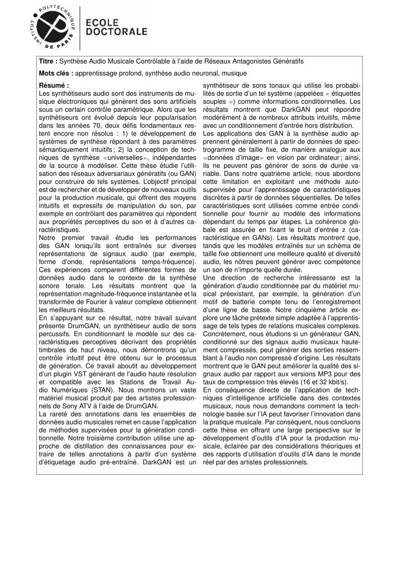
Titre : Synthese Audio Musicale Controlable a l’aide de Reseaux Antagonistes Generatifs

Mots cles : apprentissage profond, synthese audio neuronal, musique

Resume :Les synthetiseurs audio sont des instruments de mu-sique electroniques qui generent des sons artificielssous un certain controle parametrique. Alors que lessynthetiseurs ont evolue depuis leur popularisationdans les annees 70, deux defis fondamentaux res-tent encore non resolus : 1) le developpement desystemes de synthese repondant a des parametressemantiquement intuitifs ; 2) la conception de tech-niques de synthese ≪universelles≫, independantesde la source a modeliser. Cette these etudie l’utili-sation des reseaux adversariaux generatifs (ou GAN)pour construire de tels systemes. L’objectif principalest de rechercher et de developper de nouveaux outilspour la production musicale, qui offrent des moyensintuitifs et expressifs de manipulation du son, parexemple en controlant des parametres qui repondentaux proprietes perceptives du son et a d’autres ca-racteristiques.Notre premier travail etudie les performancesdes GAN lorsqu’ils sont entraınes sur diversesrepresentations de signaux audio (par exemple,forme d’onde, representations temps-frequence).Ces experiences comparent differentes formes dedonnees audio dans le contexte de la synthesesonore tonale. Les resultats montrent que larepresentation magnitude-frequence instantanee et latransformee de Fourier a valeur complexe obtiennentles meilleurs resultats.En s’appuyant sur ce resultat, notre travail suivantpresente DrumGAN, un synthetiseur audio de sonspercussifs. En conditionnant le modele sur des ca-racteristiques perceptives decrivant des proprietestimbrales de haut niveau, nous demontrons qu’uncontrole intuitif peut etre obtenu sur le processusde generation. Ce travail aboutit au developpementd’un plugin VST generant de l’audio haute resolutionet compatible avec les Stations de Travail Au-dio Numeriques (STAN). Nous montrons un vastemateriel musical produit par des artistes profession-nels de Sony ATV a l’aide de DrumGAN.La rarete des annotations dans les ensembles dedonnees audio musicales remet en cause l’applicationde methodes supervisees pour la generation condi-tionnelle. Notre troisieme contribution utilise une ap-proche de distillation des connaissances pour ex-traire de telles annotations a partir d’un systemed’etiquetage audio pre-entraıne. DarkGAN est un

synthetiseur de sons tonaux qui utilise les probabi-lites de sortie d’un tel systeme (appelees ≪ etiquettessouples ≫) comme informations conditionnelles. Lesresultats montrent que DarkGAN peut repondremoderement a de nombreux attributs intuitifs, memeavec un conditionnement d’entree hors distribution.Les applications des GAN a la synthese audio ap-prennent generalement a partir de donnees de spec-trogramme de taille fixe, de maniere analogue aux≪donnees d’image≫ en vision par ordinateur ; ainsi,ils ne peuvent pas generer de sons de duree va-riable. Dans notre quatrieme article, nous abordonscette limitation en exploitant une methode auto-supervisee pour l’apprentissage de caracteristiquesdiscretes a partir de donnees sequentielles. De tellescaracteristiques sont utilisees comme entree condi-tionnelle pour fournir au modele des informationsdependant du temps par etapes. La coherence glo-bale est assuree en fixant le bruit d’entree z (ca-racteristique en GANs). Les resultats montrent que,tandis que les modeles entraınes sur un schema detaille fixe obtiennent une meilleure qualite et diversiteaudio, les notres peuvent generer avec competenceun son de n’importe quelle duree.Une direction de recherche interessante est lageneration d’audio conditionnee par du materiel mu-sical preexistant, par exemple, la generation d’unmotif de batterie compte tenu de l’enregistrementd’une ligne de basse. Notre cinquieme article ex-plore une tache pretexte simple adaptee a l’apprentis-sage de tels types de relations musicales complexes.Concretement, nous etudions si un generateur GAN,conditionne sur des signaux audio musicaux haute-ment compresses, peut generer des sorties ressem-blant a l’audio non compresse d’origine. Les resultatsmontrent que le GAN peut ameliorer la qualite des si-gnaux audio par rapport aux versions MP3 pour destaux de compression tres eleves (16 et 32 kbit/s).En consequence directe de l’application de tech-niques d’intelligence artificielle dans des contextesmusicaux, nous nous demandons comment la tech-nologie basee sur l’IA peut favoriser l’innovation dansla pratique musicale. Par consequent, nous concluonscette these en offrant une large perspective sur ledeveloppement d’outils d’IA pour la production mu-sicale, eclairee par des considerations theoriques etdes rapports d’utilisation d’outils d’IA dans le mondereel par des artistes professionnels.

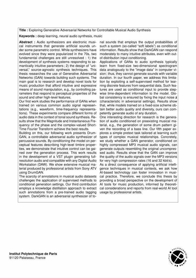
Title : Exploring Generative Adversarial Networks for Controllable Musical Audio Synthesis

Keywords : deep learning, neural audio synthesis, music

Abstract : Audio synthesizers are electronic musi-cal instruments that generate artificial sounds un-der some parametric control. While synthesizers haveevolved since they were popularized in the 70s, twofundamental challenges are still unresolved : 1) thedevelopment of synthesis systems responding to se-mantically intuitive parameters ; 2) the design of ”uni-versal,” source-agnostic synthesis techniques. Thisthesis researches the use of Generative AdversarialNetworks (GAN) towards building such systems. Themain goal is to research and develop novel tools formusic production that afford intuitive and expressivemeans of sound manipulation, e.g., by controlling pa-rameters that respond to perceptual properties of thesound and other high-level features.Our first work studies the performance of GANs whentrained on various common audio signal represen-tations (e.g., waveform, time-frequency representa-tions). These experiments compare different forms ofaudio data in the context of tonal sound synthesis. Re-sults show that the Magnitude and Instantaneous Fre-quency of the phase and the complex-valued Short-Time Fourier Transform achieve the best results.Building on this, our following work presents Drum-GAN, a controllable adversarial audio synthesizer ofpercussive sounds. By conditioning the model on per-ceptual features describing high-level timbre proper-ties, we demonstrate that intuitive control can be gai-ned over the generation process. This work resultsin the development of a VST plugin generating full-resolution audio and compatible with any Digital AudioWorkstation (DAW). We show extensive musical ma-terial produced by professional artists from Sony ATVusing DrumGAN.The scarcity of annotations in musical audio datasetschallenges the application of supervised methods toconditional generation settings. Our third contributionemploys a knowledge distillation approach to extractsuch annotations from a pre-trained audio taggingsystem. DarkGAN is an adversarial synthesizer of to-

nal sounds that employs the output probabilities ofsuch a system (so-called “soft labels”) as conditionalinformation. Results show that DarkGAN can respondmoderately to many intuitive attributes, even with out-of-distribution input conditioning.Applications of GANs to audio synthesis typicallylearn from fixed-size two-dimensional spectrogramdata analogously to the ”image data” in computer vi-sion ; thus, they cannot generate sounds with variableduration. In our fourth paper, we address this limita-tion by exploiting a self-supervised method for lear-ning discrete features from sequential data. Such fea-tures are used as conditional input to provide step-wise time-dependent information to the model. Glo-bal consistency is ensured by fixing the input noise z(characteristic in adversarial settings). Results showthat, while models trained on a fixed-size scheme ob-tain better audio quality and diversity, ours can com-petently generate audio of any duration.One interesting direction for research is the genera-tion of audio conditioned on preexisting musical ma-terial, e.g., the generation of some drum pattern gi-ven the recording of a bass line. Our fifth paper ex-plores a simple pretext task tailored at learning suchtypes of complex musical relationships. Concretely,we study whether a GAN generator, conditioned onhighly compressed MP3 musical audio signals, cangenerate outputs resembling the original uncompres-sed audio. Results show that the GAN can improvethe quality of the audio signals over the MP3 versionsfor very high compression rates (16 and 32 kbit/s).As a direct consequence of applying artificial intelli-gence techniques in musical contexts, we ask howAI-based technology can foster innovation in musi-cal practice. Therefore, we conclude this thesis byproviding a broad perspective on the development ofAI tools for music production, informed by theoreti-cal considerations and reports from real-world AI toolusage by professional artists.

Institut Polytechnique de Paris91120 Palaiseau, France