Exploring B-ISDN Performance Interactions

NTIA Report 96-329

Exploring B-ISDN Performance Interactions:Selected Experiments and Results

D.J. Atkinson

U.S. Department of CommerceMickey Kantor, Secretary

Larry Irving, Assistant Secretaryfor Communications and Information

April 1996

(This page intentionally left blank.)

iii

PREFACE

Funding for this work was provided jointly by the U.S. Department of Commerce and theNational Communication System (NCS). The work was conducted at the Institute forTelecommunication Sciences under the supervision of W. R. Hughes. Technicalmanagement for the NCS funding was provided by G. Kelley.

The author wishes to express gratitude to U S West for the opportunity to participate intheir ATM networking trial, and specifically J. Meissner and P. O’Connor for theirexcellent technical support during the trial. Also, thanks are due to R. Bloomfield, whoreviewed this document multiple times and provided insightful commentary to assist inimproving it.

Certain products, companies and organizations may be mentioned in this report toadequately explain the experiments and their results. In no case does such identificationimply recommendation or endorsement by the National Telecommunications andInformation Administration, nor does it imply that those identified are necessarily the bestavailable for this work.

iv


v

CONTENTS

page

PREFACE . . . . . . . . . . . . . . . . . . . . . . . . . . . . . . . . . . . . . . . . . . . . . . . . . . . . . . . . . . . . . . . iii

ABSTRACT . . . . . . . . . . . . . . . . . . . . . . . . . . . . . . . . . . . . . . . . . . . . . . . . . . . . . . . . . . . . . . . 1

1. INTRODUCTION . . . . . . . . . . . . . . . . . . . . . . . . . . . . . . . . . . . . . . . . . . . . . . . . . . . . . . . . 11.1 B-ISDN: The Emerging Telecommunications Infrastructure . . . . . . . . . . . . . . 11.2 The Importance of B-ISDN . . . . . . . . . . . . . . . . . . . . . . . . . . . . . . . . . . . . . . . . . . 41.3 Report Organization . . . . . . . . . . . . . . . . . . . . . . . . . . . . . . . . . . . . . . . . . . . . . . . 6

2. ASSESSING B-ISDN USER INFORMATION TRANSFER PERFORMANCE . . . . . . . 82.1 Physical Layer (Recommendation G.826) . . . . . . . . . . . . . . . . . . . . . . . . . . . . . . 82.2 ATM Layer (Recommendation I.356) . . . . . . . . . . . . . . . . . . . . . . . . . . . . . . . . 10

3. DEVELOPING A TOOL TO STUDY B-ISDN PERFORMANCE . . . . . . . . . . . . . . . . . 133.1 B-ISDN Network Emulator . . . . . . . . . . . . . . . . . . . . . . . . . . . . . . . . . . . . . . . . 133.2 External Interfaces . . . . . . . . . . . . . . . . . . . . . . . . . . . . . . . . . . . . . . . . . . . . . . . 173.3 Developing an Error Model . . . . . . . . . . . . . . . . . . . . . . . . . . . . . . . . . . . . . . . . 19

4. VALIDATING THE B-ISDN NETWORK EMULATOR . . . . . . . . . . . . . . . . . . . . . . . . 224.1 Purpose of the Validation Experiment . . . . . . . . . . . . . . . . . . . . . . . . . . . . . . . 224.2 Experiment Description . . . . . . . . . . . . . . . . . . . . . . . . . . . . . . . . . . . . . . . . . . . 224.3 Requirements for Validation . . . . . . . . . . . . . . . . . . . . . . . . . . . . . . . . . . . . . . . 234.4 Discussion of Results . . . . . . . . . . . . . . . . . . . . . . . . . . . . . . . . . . . . . . . . . . . . . 244.5 Conclusions Derived from the Validation Experiment . . . . . . . . . . . . . . . . . . 28

5. RELATING PHYSICAL- AND ATM-LAYER PERFORMANCE . . . . . . . . . . . . . . . . 305.1 Case 1: Scattered ES with Sync Loss . . . . . . . . . . . . . . . . . . . . . . . . . . . . . . . . . 315.2 Case 2: Clumped ES with Sync Loss . . . . . . . . . . . . . . . . . . . . . . . . . . . . . . . . . 325.3 Case 3: Scattered ES with High BER . . . . . . . . . . . . . . . . . . . . . . . . . . . . . . . . . 335.4 Case 4: Clumped ES with High BER . . . . . . . . . . . . . . . . . . . . . . . . . . . . . . . . . 345.5 Performance Comparisons . . . . . . . . . . . . . . . . . . . . . . . . . . . . . . . . . . . . . . . . . 34

6. STUDYING PERFORMANCE OF A PROTOTYPE ATM NETWORK . . . . . . . . . . . . 376.1 Network Trial: Initial Architecture . . . . . . . . . . . . . . . . . . . . . . . . . . . . . . . . . . 376.2 Network Trial: Second Phase . . . . . . . . . . . . . . . . . . . . . . . . . . . . . . . . . . . . . . . 416.3 Discussion and Conclusions . . . . . . . . . . . . . . . . . . . . . . . . . . . . . . . . . . . . . . . 47

vi

7. RELATING PHYSICAL-LAYER PERFORMANCE TO VIDEO QUALITY . . . . . . . . 497.1 Experiment Description . . . . . . . . . . . . . . . . . . . . . . . . . . . . . . . . . . . . . . . . . . . 497.2 Results . . . . . . . . . . . . . . . . . . . . . . . . . . . . . . . . . . . . . . . . . . . . . . . . . . . . . . . . . 517.3 Discussion of Results . . . . . . . . . . . . . . . . . . . . . . . . . . . . . . . . . . . . . . . . . . . . . 56

8. SUMMARY . . . . . . . . . . . . . . . . . . . . . . . . . . . . . . . . . . . . . . . . . . . . . . . . . . . . . . . . . . . . 58

9. REFERENCES . . . . . . . . . . . . . . . . . . . . . . . . . . . . . . . . . . . . . . . . . . . . . . . . . . . . . . . . . . 60

APPENDIX A. ACRONYMS AND ABBREVIATIONS . . . . . . . . . . . . . . . . . . . . . . . . . . 63

APPENDIX B. OVERVIEW OF B-ISDN . . . . . . . . . . . . . . . . . . . . . . . . . . . . . . . . . . . . . . . 65

APPENDIX C. PERFORMANCE DATA FROM INITIAL PHASE OF TRIAL NETWORK . . . . . . . . . . . . . . . . . . . . . . . . . . . . . . . . . . . . . . . . . . . . . . . . . . . . . . . . 81

APPENDIX D. PERFORMANCE DATA FROM SECOND PHASE OF TRIAL NETWORK . . . . . . . . . . . . . . . . . . . . . . . . . . . . . . . . . . . . . . . . . . . . . . . . . . . . . . . . 99

The author is with the Institute for Telecommunication Sciences (ITS), National*

Telecommunications and Information Administration (NTIA), U.S. Department ofCommerce, 325 Broadway, Boulder, CO 80303-3328.

EXPLORING B-ISDN PERFORMANCE:SELECTED EXPERIMENTS AND RESULTS

D.J. Atkinson*

ABSTRACT

This report describes experiments conducted to explore the user-informationtransfer performance of the broadband integrated services digital network(B-ISDN), the emerging infrastructure for the global information age. Theseperformance experiments include studying the effect of physical layertransmission performance on asynchronous transfer mode (ATM) celltransfer performance, ATM performance in relationship to networktopology, and the impact of B-ISDN performance on video quality. A toolto help study these performance issues, a B-ISDN network emulator, isdescribed, including its validation. The emulator incorporates a novel modelfor transmission impairments, enabling performance interactions among theB-ISDN protocol layers to be studied based on relevant InternationalTelecommunication Union - Telecommunication Standardization Sector(ITU-T) Recommendations and American National Standards.

Keywords: asynchronous transfer mode; ATM; B-ISDN; broadband; emulation;measurement; network; performance; SONET; standards; synchronousoptical network

1. INTRODUCTION

1.1 B-ISDN: The Emerging Telecommunications Infrastructure

The broadband integrated services digital network (B-ISDN) has been cited as the “master

plan” for the emerging digital telecommunications infrastructure that will provide

advanced high-performance voice, video, data and integrated multimedia services to users

on a worldwide basis [1]. Indeed, B-lSDNs are expected to be a principal component of

the Global Information Infrastructure (GII) proposed by U.S. representatives at the World

Telecommunications Development Conference held by the International

2

Telecommunication Union (ITU) in March 1994 [2]. Recent international conferences

continue to emphasize the importance of B-ISDN within the context of GII development

and its national counterparts (e.g., U.S. National Information Infrastructure, NII; European

Information Infrastructure, EII) [3].

The B-ISDN concept utilizes a unifying architecture and framework for integrating several

innovative technologies (e.g., fiber optic transmission and computer-based switching) in

efficient, interoperable public and private networks that will provide dramatic

improvements in telecommunications capacity, flexibility, and performance to users.

Many international experts agree that the advanced services engendered by B-ISDN

deployment will be essential to ensure a country's economic prosperity and

competitiveness in the global marketplace. Also important is the enhancement of the

security and well-being of citizens by promoting more efficient and effective provision of

social services, including law enforcement, environmental protection, health care, and

national defense. It can strengthen the social fabric by extending the benefits of high-

quality education to all citizens, enriching and stimulating lives through innovation in all

forms of communication.

B-ISDN information transport is via the asynchronous transfer mode (ATM). This cell-

based multiplexing technology gives network providers the unprecedented transmission-

capacity-allocation flexibility required to meet increasingly diverse user needs. The ability

to switch high-bit-rate streams of user data enables the provision of new services, such as

high-quality video telephony and teleconferencing, tele-shopping, remote banking, tele-

medicine, on-demand video and audio entertainment, interactive multiparty games, and

electronic publications.

Technical standards (“Recommendations” ) developed in the ITU's Telecommunication

Standardization Sector (ITU-T) provide the “blueprints” that define B-ISDN technologies

The ITU-T plays a preeminent role in the cooperative planning of global public1

telecommunications systems and services. The Recommendations developed in the ITU-Thave substantial impact on both the evolution of the U.S. telecommunicationsinfrastructure and the international competitiveness of U.S. products and services. TheInstitute for Telecommunication Sciences (ITS) supports ITU-T activities by leading U.S.preparatory committees and international work groups, preparing technical contributionsto advance ITU-T standards development, and drafting proposed Recommendations ontopics of importance to U.S. interests. This report was developed in conjunction with ITS’international standards activities.

3

and services. An initial set of 13 I-series Recommendations defining essential B-ISDN1

characteristics was approved by CCITT (now ITU-T) in December 1990. This set of

Recommendations has evolved into a broad family of ITU-T standards that collectively

provides a detailed specification of B-ISDN transport technology, including network

architectures (I.100 series), services (I.200 series), network capabilities (I.300 series), user-

network and network-network interfaces (I.400 and I.500 series), operations and

maintenance facilities (I.610 series), and equipment (I.700 series). American National

Standards Institute (ANSI)-accredited Committee TI (Telecommunications) contributed

strongly to the development and coordination of the I-series Recommendations and has

developed over a dozen American National Standards (T1.600 series) that affirm,

elaborate, and specialize them for application in North America.

These B-ISDN/ATM cell transfer standards developed in ITU-T and Committee T1 have

already had a profound impact on network planning and are being implemented in

commercial products and services in many countries; however, there is still more to be

done. Current standards development is focused in three areas. First is the development

of advanced B-ISDN /ATM signaling protocols that will allow users to establish

multipoint connections and multiconnection calls and to change dynamically the capacity

or performance of connections to meet their specific communication needs. Second is the

specification of traffic management standards that will allow network managers to access

the full flexibility of ATM resource allocation in meeting their users' needs. Finally, there

This report assumes the reader has a general knowledge of the B-ISDN standards and2

Recommendations. A brief overview of B-ISDN is provided in Appendix B. More detailedinformation can be found by referring to the citations in the bibliography for thatAppendix.

4

is a need to develop advanced standards for performance measurement to enable users

and providers to quantify the improvements observed by using B-ISDN and to promote

more effective matching of offered systems and services with user needs. It is this last

topic that motivates the technical study documented in this report.2

1.2 The Importance of B-ISDN

B-ISDN creates the potential for a global information infrastructure that could empower

nations and enrich societies worldwide. However, the technological advances have

created a striking abundance of product alternatives and an industry environment of

unprecedented complexity, making it difficult to match user requirements to specific

technology and service solutions. An essential means of addressing this challenge is the

standardization of telecommunication service quality measures [4]. These measures

provide the common ground necessary for communication among service providers and

users, allowing providers to design and implement telecommunication systems and

services and users to define telecommunication requirements and select the products that

most effectively meet them [5].

Telecommunication performance standards generally have three parts: performance

parameters, measurement methods, and performance objectives. Performance parameters

and their definitions are the measurable characteristics of the network that can have an

impact on the overall perception of the network quality. Measurement methods are means

of estimating the parameter values. They are standardized to ensure that the performance

parameters are computed correctly and/or always computed in a manner that will give

consistent results from network to network. Finally, performance objectives may be

5

standardized to facilitate the procurement of competitively offered services or as metrics

for equipment manufacturers.

Performance measurement standards generally are addressed to one of two audiences:

users or providers. Since telecommunication services exist to fulfill the needs of users, it

is important to specify and measure the quality of telecommunication services using

performance measurement standards that provide a means for a user to express their

satisfaction (or dissatisfaction) with the delivered service. Such performance measurement

tools are described as “user-oriented.” User-oriented parameters, often referred to as

“quality-of-service,” differ from the provider-oriented network performance parameters

traditionally used in network design and operation, both in where they are applied and

how they are defined [6].

The user-oriented parameters are applied at user interfaces, which typically are more

inclusive than the interfaces between the network provider and the customer premises

equipment. Developing parameters for application at the user's interface ensures that

parameters are observable and relevant to the user. Users of network services are not

intrinsically interested in how the services are implemented, the networks' internal cause

of externally observable service degradations, or the network's architecture. They are,

however, interested in limiting the observable effects of network imperfections and in

comparing network service alternatives.

Currently, performance measurement standards have been adopted for two layers of the

B-ISDN protocol model: the physical layer [7,8] and the ATM layer [9,10]. In order to

relate the performance of these provider-oriented standards to user needs and

requirements, it is essential that the interactions between the different layers of the system

be studied (Figure 1). Questions such as, “What happens to video when an ATM cell is

dropped or the physical layer loses synchronization?” need to be answered to help users

6

Figure 1. Measurement points for provider- and user-oriented performance parameters [4].

determine how B-ISDN can best meet their needs as well as help network providers design

and implement cost-effective competitive systems. Answers to this, and related questions,

provide a “vertical integration” of performance information, giving network providers the

long-sought-after means of relating network performance impairments (or enhancements)

with the performance perceptions (and practical application decisions) of their customers.

The limited availability of B-ISDN performance information further reinforces the need

to study performance interactions within and among the various layers of the B-ISDN

system.

1.3 Report Organization

This report addresses the need for more information on the performance of B-ISDN by

1) describing a tool, based on existing performance measurement standards, that can be

used to assist in such studies; and 2) demonstrating its utility through the conduct of

several experiments. This tool, a B-ISDN network emulator (BNE) is used to

- explore B-ISDN performance under a variety of network conditions,

7

- obtain information about the physical- and ATM-layer performance that might beexpected based on existing performance objectives,

- analyze the performance of a trial ATM network, and- examine video performance when the signal is passed through both the BNE and

the prototype network.

While the paths may be based on a plesiochronous digital hierarchy, synchronous3

digital hierarchy, or some other transport network (e.g., cell based), the Recommendationis generic in that it defines parameters and objectives independent of the physical transportnetwork providing the paths. The Recommendation uses a block-based measurementconcept using error detection codes inherent to the paths under test.

These objective apply to each direction of a 27,500-km hypothetical reference path and4

are intended to satisfy the future needs of the digital networks. Therefore they may notbe readily achieved by all of today’s digital equipment and systems.

8

2. ASSESSING B-ISDN USER INFORMATION TRANSFER PERFORMANCE

The ITU has addressed B-ISDN user information transfer performance assessment through

the July 1993 adoption of Recommendations G.826 and I.356. Recommendation G.826

defines error performance parameters and objectives for international digital paths that

operate at or above the primary rate. Recommendation I.356 defines parameters for

assessing ATM-layer user information (cell) transfer performance. Performance objectives

for the ATM layer have not yet been determined, but provide a focus for standardization

work in the ITU-T (Question 16/13) and in ANSI-accredited Technical Subcommittee T1A1

(Working Group T1A1.3 - Performance of Digital Networks and Services).

2.1 Physical Layer (Recommendation G.826)

The physical-layer performance parameters defined in Recommendation G.826 are

summarized in Table 1. These parameters, background block error ratio (BBER), errored

second ratio (ESR), and severely errored second ratio (SESR), provide information on the

error performance of constant-bit-rate digital paths . Recommendation G.826 specifies3

end-to-end performance objectives for BBER, ESR, and SESR as a function of the bit rate4

of the path; however, this report is only concerned with the objectives for paths operating

at 155 Mbit/s.

STM-1 refers to the SDH designation of a 155.52 Mbit/s channel. The SONET5

designator for this bit rate is STS-3 or STS-3c, depending on overhead configuration. Atthis bit rate, there are 19,440 bits (including overhead) per frame.

9

Table 1. G.826 Performance Parameters and Their Definitions*

Parameter Definition

Background Block The ratio of errored blocks to total blocks during a fixedError Ratio (BBER) measurement interval, excluding all blocks during severely

errored seconds and unavailable time. For SONET/SDH(Synchronous Optical Networks/Synchronous DigitalHierarchy) networks a block is considered equivalent to aSONET/SDH frame.

Errored Second The ratio of errored seconds to total seconds in available timeRatio (ESR) during a fixed measurement interval. An errored second is a

one second period with one or more errored blocks.

Severely Errored The ratio of severely errored seconds to total seconds inSecond Ratio (SESR) available time during a fixed measurement interval. A

severely errored second is a one second period that contains30% or more errored blocks, or at least one network defect.

The performance parameter definitions provided in this table are from the 1993*

version of Recommendation G.826. The ITU has adopted a policy whereRecommendations can be revised as often as every two years. If the reader wishes toconduct performance measurements, the current version of the Recommendationshould be obtained to ensure that the parameter definitions used are correct.

The objectives for paths of that speed are as follows:

BBER 0.00020ESR 0.160SESR 0.0020

In this report, a block size equivalent to one synchronous transfer mode level 1 (STM-1)5

frame is used to measure G.826 defined parameters.

10

2.2 ATM Layer (Recommendation I.356)

Table 2 shows the possible performance-significant outcomes that a cell can have in an

ATM connection as defined in ITU-T Recommendation I.356. These outcomes are used to

develop the ATM-layer performance parameters summarized in Table 3.

Although performance objective have been specified for the physical layer, (see Section

2.1), objectives have not yet been set for ATM-layer cell transfer performance. However,

once set, the objectives will not differentiate the sources of performance degradations (i.e.,

the effects of physical-layer performance and ATM-switch performance will be included

in the objective). As each experiment is conducted, the appropriate parameters and the

relationships between parameters at the various layers will be considered. ATM-layer

performance parameters are not specified during intervals where the ATM cell transfer

service is considered unavailable or when nonconforming user cells are transmitted.

Looking at the definitions, on can conjecture about the relationship between the physical-

layer parameters and the ATM-layer parameters. For example, some ATM-layer

parameters, such as cell delay variation (CDV), should only be minimally affected by

physical-layer performance. The physical layer introduces relatively constant cell transit

delay (CTD), but there is some variation (about 500 nanoseconds) introduced through

packing the ATM cells in amongst the SONET/SDH overhead. It is the delay experienced

in ATM switch queues that should provide the most significant contribution to CDV. Cell

loss ratio (CLR) should usually only be affected by physical-layer performance if the

header error control (HEC) function of ATM is disabled. If the HEC function is enabled,

the forward nature of the error correction function means that many cell losses caused by

physical-layer performance to occur in severely errored cell blocks. Mean CTD is affected

by the physical layer, but is fixed in the laboratory equipment, regardless of the change in

other performance factors. These conjectures for the basis for the performance experiments

conducted and reported in the following sections of this report.

11

Table 2. Recommendation I.356 Transfer Outcomes for an ATM User Cell*

Cell Outcome Definition

Successful sent, 2) with a valid header, and 3) within a specified maximumA cell is received 1) with a payload matching the payload that was

transfer time.

Errored errors, or 2) with an invalid header (after HEC proceduresA cells is received 1) with a payload that contains one or more

completed) but still within a specified maximum transfer time.

LostA cell is not received within a specified maximum transfer time,excluding those cells lost by customer equipment.

Misinserted A cell is received that has no corresponding transmitted cell.

Severely errored More than a specified number (M) of errored, lost, or misinsertedcell block cells occur in a block of N consecutive cells in a connection.**

The definitions summarized here are from the 1993 version of Recommendation I.356.*

In the version of Recommendation I.356 in force at the time of testing, values for M and**

N were listed “for further study.” Provisional values for M and N, based on peak cellrate, are provided in the 1996 revision of I.356. For example, in an ATM connectionusing the full capacity of an STM-1 (353,208 cells per second), N=16,384 and M=512 isspecified.

12

Table 3. I.356 Performance Parameters and Their Definitions*

Parameter Definition

Cell Error Ratio (CER) The ratio of total errored cells to total successfully transferredcells plus errored cells in a population of interest.Transmitted cells that are part of a severely errored cell blockare excluded from the population.

Cell Loss Ratio (CLR) The ratio of total lost cells to total transmitted cells in apopulation of interest. Transmitted cells that are part of aseverely errored cell block are excluded from the population.

Cell Misinsertion Rate The total number of misinserted cells observed during a(CMR) specified time interval divided by the duration of the

interval. Misinserted cells and time intervals associated withseverely errored cell blocks are excluded when calculatingthe value of this parameter.

Severely Errored Cell The ratio of total severely errored cell blocks to total cellBlock Ratio (SECBR) blocks in a population of interest.

Mean Cell Transfer The arithmetic average of a specified number of cell transferDelay (CTD) delays. Cell transfer delay is the (positive) difference

between the time when a successfully transferred cell entersthe network and when it exits the network.

Cell Delay Variation 1. One point definition: if the cells are inserted into the(CDV) network at regular intervals, this is the variation in the

interval between cell exits. 2. Two point definition: thevariation in individual cell transfer delays (the two-pointdefinition is used exclusively in the performance datapresented in this report).

Cell Flow Parameters The parameters for measuring cell flow through the networkare under study.

*The definitions summarized here are from the 1993 version of Recommendation I.356.

13

3. DEVELOPING A TOOL TO STUDY B-ISDN PERFORMANCE

As the Institute for Telecommunication Sciences (ITS) undertook the development of a B-

ISDN network emulator (BNE) to conduct physical- and ATM-layer performance studies,

it became clear that not all capabilities would be available at once. Thus, it seemed logical

to develop the device in phases. Phase 1 implemented internal ATM cell generation

capabilities and controlled physical-layer error generation capabilities to study the effects

of physical-layer performance on the internally-generated ATM cell stream. Phase 2

added functionality to study the performance effects on applications that generated traffic

external to the BNE.

The basic hardware and software platforms used in developing the BNE were obtained

commercially. Although this approach may limit flexibility somewhat, there is significant

benefit in using commercial products - notably, reduced cost. The labor and time required

to design, construct, and validate a SONET/ATM test system “from scratch” would be

substantial.

The specific computer programs used to control the experiments reported here were

developed at ITS. These ITS-developed test programs significantly supplemented those

available from the manufacturer and were essential for achieving the full emulation and

measurement capabilities of the BNE.

3.1 B-ISDN Network Emulator

In Phase 1, the BNE was a closed system as shown in the block diagram in Figure 2. All

of the components, except the controller, were integrated into a single VXI card cage. The

controller was connected to the card cage via GP-IB (General Purpose Instrumentation

Bus).

14

Figure 2. BNE during Phase 1.The simplest system components to describe are the optical transmitter and receiver. Each

of these modules has one function: conversion between an electrical signal and an optical

signal. No protocol work is required as all protocol information is encoded prior to arrival

at the optical transmitter, and the optical receiver leaves it intact when it passes the stream

to the transport overhead (TOH) receiver. The optical interfaces on these cards use a

1310-nm laser to communicate over single mode fiber. This fiber is connected to the

modules via an FC/PC connector. On the other side, the electrical connections consist of

two SMA connectors per module, one for data and one for a clock signal.

The TOH generator is significantly more complex. This module is responsible for adding

the additional protocol to an ATM cell stream required to make a SONET or SDH stream.

A number of TOH parameters can be controlled by the operator. Two particularly useful

operator controls are the ability to turn the frame scrambler on and off, and bytewise

programming of the transport and path overhead. Equally important is the ability to

create impairments in the stream of data passed to the optical transmitter. The impairment

generator can add the following impairments.:

This is true for an STS-3c or STM-1 physical layer used for the experiments presented6

in this report.

15

- frameword errors,- alarm signals,- automatic protection switching signals,- parity byte errors,- Poisson-distributed bit errors in either the overhead portion of the frame, or

across the whole frame.

The bit error generator provided with the basic emulator can generate errors only at ratios

from 10 through 10 in decades. The emulator controller can change the error ratio at-9 -2

approximately 18 ms intervals. The ATM stream is input to this module via the VXI card

cage bus, and output through two SMA connectors (one each for data and clock signals).

As might be expected, the TOH receiver has similar, but opposite responsibilities to those

of the TOH generator. Rather than adding the SONET or SDH protocol, it strips it off.

Rather than generating errors, it measures them. The impairments that can be measured

by the TOH receiver module include pointer errors, parity byte errors, framing errors, and

alarms. As with the TOH generator, connections are made via SMA connectors for the

SONET/SDH-formatted stream and the VXI backplane for the raw ATM stream.

Much of the functionality of the ATM generator module is related to impairment

generation; however for Phase 1 testing, the sole purpose of this module is to provide a

continuous stream of valid ATM cells. These cells are filled with pseudo random data,

segmented in accordance to ATM Adaptation Layer 1 (AAL1) standards, and provided to

the TOH generator at the maximum allowable data rate of 149.76 Mbit/s . It provides this6

stream of ATM cells to the TOH generator via the VXI bus.

While many of the error generation capabilities of the ATM generator are not used in this

experiment configuration, many of the error analysis functions on the ATM receiver are

16

used. Once the ATM stream is received from the TOH receiver, the module analyzes it to

determine if any of the following impairments have occurred in the ATM stream:

- noncorrectable header errors,- lost cells,- pseudorandom sequence errors (i.e., data errors),- alarm indicators,- cell sequence number errors, or- loss of cell synchronization.

Any of these errors can occur from physical-layer impairments.

The final component of the system is the emulator controller. The emulator controller is

the “brain” behind the entire system and performs both controlling and recording

functions. The controller is programmable in the “C” programming language, and

communicates with the other components of the system via a GP-IB. During an

experiment, the controller initializes the components, creates impairments as directed by

the error model (described below), and saves all relevant data to a file. Once the

experiment is finished, the data can be analyzed off-line, and performance parameters can

be calculated. The programs written to control the network emulator are essential to its

utility. Without them, all settings would have to be made manually, and could not be

changed rapidly enough to provide a realistic error model. Also, without the additional

software, the device would have to be instructed manually to extract and record

measurements at each desired measurement interval.

A closed system such as the one described has limited uses, but very important among

those uses is the ability to function in a totally controlled environment. A controlled

environment is essential for validating the BNE and adjusting the parameters in the error

model. These items are discussed Sections 4 and 5, respectively, of this report.

Audio I/O

Video I/O

Data I/O

DS-3

H.261

CODEC

ATMService

Multiplexer

DS-1

OC-3

OpticalTransmitter

Generator

TOH

Error

ControllerEmulator

Audio I/O

Video I/O

Data I/O

CODEC

DS-3

OC-3

ReceiverOptical

Receiver

TOHGenerator

ATMReceiver

w/ T1 CSU/DSU

17

Figure 3. B-ISDN emulator during Phase 2.

3.2 External Interfaces

The usefulness of the emulator was increased substantially by adding external interfaces.

The hardware configuration is shown in Figure 3. The components within the box are the

same as those described in the previous section; however, this configuration takes

advantage of the transport overhead generator's and receiver's ability to exchange payload

data via the VXI bus, rather than through the external interfaces, as shown in Figure 2.

Like the hardware mentioned in the previous Section, all components described here are

commercially available.

The most significant component required to complete this phase of the BNE is the service

multiplexer. This device supports the multiplexing of DS-1 and DS-3 plesiochronous data

A virtual connection is indicated by the address in the header of the ATM cell, a7

combination of the virtual path identifier and the virtual channel identifier. For a PVC, theaddresses are predefined, and the connection is always open.

A 4.5-MHz video signal sampled at 9 MHz (Nyquist frequency) at 8 bits/sample would8

be 72 Mbit/s. More typical is sampling at 14.3 MHz (four times the 3.58 MHz subcarrierfrequency) for a data rate of 114.4 Mbit/s. If more bits per sample were required, thatwould also increase the required bit rate.

18

streams onto a SONET STS-3c/ATM channel. Each plesiochronous data stream is assigned

to a permanent virtual connection (PVC). This PVC can be routed through the network7

impairment generator, a real network, or a hybrid network that consists of both. This

allows for maximum test flexibility.

Also important is the addition of “live” data sources. In this case, two video

coder/decoders (codecs) that operate at significantly different bit rates were chosen. The

first codec conforms to ITU-T Recommendation H.261. This Recommendation provides

for coding of video at multiples of 64 kbit/s, up to 2.048 Mbit/s; however, the CSU/DSU

(channel service unit/data service unit) limits the maximum bit rate of the codec used in

the BNE to 1.536 Mbit/s. Because of the high compression ratio (uncompressed video

requires 72 Mbit/s or more depending on required fidelity [11] ), the video output from8

the decoder contains numerous artifacts. Included among these are blocking, blurring,

slow frame rate (and the resulting jerky motion), and reduced frame size. The codec also

provides audio coding capability at several bit rates and quality levels, and a data

communications capability.

The second codec operates at a significantly higher bit rate (approximately 45 Mbit/s). The

corresponding reduction in compression ratios allows this codec to deliver much higher

quality video. Even so, the proprietary coding algorithm does introduce some artifacts.

These are generally most visible near sharp vertical edges, which can appear slightly

It is not common to have a time driven state machine with a variable state time.9

Therefore, it might help the reader to consider that the state time is 19 ms (half waybetween the maximum and minimum values) with an accuracy of ±2 ms.

19

jagged or contain some noise. This codec can also incorporate stereo audio and low bit rate

data into the 45-Mbit/s stream.

3.3 Developing an Error Model

In order for the BNE to introduce meaningful degradations into a SONET/ATM channel,

it is necessary to use an algorithm, or model, to introduce those degradations. This error

model must work within the limitations in the types of bit errors that can be introduced

by the impairment generator. The errors are limited to a Poisson distribution with error

ratio s from 10 through 10 in decades. This by itself is not particularly useful. However,-9 -2

using software control, it is possible to change the bit error ratio (or turn it off) at intervals

of 17-21 ms, with the overall average being about 18 ms. Assuming the physical layer will

stay at a given error ratio longer than these intervals, this can be used to create a time-

driven state machine. The state machine implemented in this study to emulate9

transmission impairments is a Markov chain.

There are several conditions that define a Markov chain. The most basic definition

involves a set of states and a set of transition probabilities that govern movement between

states. These probabilities are generally defined as p , the probability of a transition fromij

state i to state j (i being the current state and j being the next state). This implies another

condition of a Markov chain: the probability of a given state occurring next is determined

solely by knowledge of the current state, and not from any knowledge of previous states.

To be more precise, the probability of state s occurring at time t+1 (for t greater than or

equal to 1) is the same regardless of whether only the current state is known, or if the

entire state history is known. Stating this mathematically,

for t�1, P{ st�1 st } = P{ st�1 st, st1, # # # , s1 }

P =

p11 p12 p13 p14

p21 p22 p23 p24

p31 p32 p33 p34

p41 p42 p43 p44

.

20

Figure 4. Four state Markov chain.

where s is the state at time t.t

A four state Markov chain, with all transitions labeled, is shown in Figure 4. This chain

is governed by the transition matrix (P) where

The flow of the model between states can be changed by adjusting the transition

probabilities. However, the sum over j of p must equal 1.ij

With the ability to use transition probabilities to control the flow from one state to the next

comes the utility required to

emulate specific network

conditions. For ITS work, the

Markov chain was used to create

a certain level of physical-layer

performance. Once the BNE

was validated, experiments

used a four state Markov chain

to accomplish this. The initial

state, and the state in which the

chain spends the most time, is a

zero error state. The remaining

21

time is divided among the other three states. Two of these states have bit error ratios

(BERs) in the range of 10 to 10 . The fourth state is a severely errored state such as 10-5 -8 -2

BER or service outage. Previous work has shown that this generic model is somewhat

representative of the errors found in optical systems [12]. However, as more data becomes

available on the physical-layer performance, the model can be updated as necessary.

In the experiments described in this report, several of these chains were used to provide

a variety of network impairments. These impairments include a variety of burstiness in

the errors, as well as different types of severe impairments. The transition probabilities

and error conditions for each chain are detailed with the experiment relevant to that chain.

22

4. VALIDATING THE B-ISDN NETWORK EMULATOR

4.1 Purpose of the Validation Experiment

Before the system described in previous sections could be applied to studies of specific

performance issues, it was necessary to demonstrate that the BNE operated correctly under

known, or predictable conditions. An experiment was therefore conducted to confirm

basic information about the effect of distributed errors at the physical layer on ATM

performance, including the effect of using the HEC and scrambling functions of ATM.

4.2 Experiment Description

The experiment introduced bit errors, according to a Poisson distribution, into the

physical-layer channel. It is recognized that this distribution of errors is not likely to occur

in a “real” ATM network [12]. However, using this distribution of errors is sufficient for

this experiment, in that it provides simple predictable conditions that can be used to

validate the functionality and utility of the test equipment.

During the experiment, errors were introduced at a variety of BERs. The applied BERs

were 0 and 10 through 10 in increments of powers of 10. This provided a total of 9 levels-9 -2

of error. For each ER applied to the physical channel, performance parameters were

calculated for the physical layer and the ATM layer. For the physical layer, BBER, ESR,

and SESR were calculated. For the ATM layer, CLR and CER were calculated. These

parameters were calculated as defined in Recommendation G.826 (for physical-layer

performance) and Recommendation I.356 (for ATM-layer performance) and summarized

in Section 2. The only exception to this was that the SECBR was not calculated prior to the

CER. (Recall that CER does not normally include cells that are part of a severely errored

cell block.) This had no effect at the lower error ratios, because the distributed errors do

not cause severely errored cell blocks until the BER is greater than 10 . The effect on higher-5

User Bit Error Ratio = Number of Errored User Bits DeliveredTotal User Bits Transmitted� Lost User Bits

23

error ratios is determined by the percentage of errored cells required to constitute a

severely errored cell block. This topic will be discussed in greater detail in Section 4.4.

In addition to the G.826 and I.356 parameters, a “user” BER was calculated from the data

transported by the ATM layer to the AAL. This BER was calculated in order to verify that

the scrambling function in the emulator behaves in accordance with ITU-T

Recommendation I.432 [13]. (The nature of the ATM scrambling function and ATM HEC

function is explained in Appendix B.4.) The parameter was calculated according to the

following formula:

4.3 Requirements for Validation

In order for the test equipment to be declared valid for use in more complex experiments,

the following phenomena should be observed during the experiment described above:

1) When the ATM scrambling function is disabled, the user BER should be

equivalent to the introduced physical-layer BER. This is because a specific

error ratio introduced into a channel will cause any subchannel to have the

same error ratio if there is no error correction or other processes affecting the

data in that subchannel.

2) When the physical-layer scrambling function is enabled, the user BER should

be doubled when compared to the user BER without the scrambling function.

3) The CER should be 384 times the introduced physical-layer BER until that BER

is approximately 4*10 . There are 384 bits in an ATM cell not protected by error-3

correction. If there are N bits from one errored bit to the next, there are N/384

24

cells from one errored cell to the next. Using the subchannel principle

mentioned above, the CER becomes 384 times the BER. As the BER approaches

4*10 , N/384 approaches 1.0, and the estimation method breaks down.-3

4) When the HEC function is disabled, the cell loss ratio should be 40 times the

introduced physical-layer BER. When the HEC function is disabled, the 40

header bits of an ATM cell are no longer error-protected. When one of these

40 bits is errored, the cell is discarded and reported as lost. Using the

principles mentioned above, the CLR becomes 40 times the BER.

5) When the HEC function is enabled, the Poisson error model should allow

virtually zero cell loss up to a physical-layer BER of 10 , because almost all-3

errored headers will have only one error, a correctable condition. Even after

the BER exceeds that point, the cell loss ratio should be significantly lower than

when the HEC function is not used because many of the headers will still only

have one error.

If these conditions are met, within explainable differences, thethe BNE is considered to be

functioning properly at a basic level, and can be applied to more complex error modeling

scenarios.

4.4 Discussion of Results

4.4.1 Physical Layer

Table 4 shows the experimental results of distributed errors on measured G.826

performance parameters. Upon examination of the table, it is apparent that the errors

introduced into the system saturate the ESR and BBER relatively early in the experiment.

ESR is near the performance objective (0.16) at a bit ER of 10 , and BBER is near the-9

performance objective (0.0002) at a bit ER of 10 . Also, because of the nature of the error-8

25

Table 4. G.826 Performance Parameter Values Resulting from Poisson-distributed Errorsin the Physical Channel*

SDH Bit ER BBER ESR SESR

0 0 0 0

10 1.92*10 0.153 0-9 -5

10 1.94*10 0.99 0-8 -4

10 1.94*10 1 0-7 -3

10 1.94*10 1 0-6 -2

10 1.94*10 1 0-5 -1

10 undefined 1 1-4

10 undefined 1 1-3

10 undefined 1 1-2

No physical-layer scrambling was used in collecting this data.*

model, there are no intermediate values for the SESR. At a bit ER of 10 , SESR jumps from-4

0 to 1, due to the definition of a severely errored second ( � 30% errored blocks ). At this

point, there are no seconds that are not severely errored, and therefore BBER becomes

undefined.

Examination of the experimental results provides some information that is outside the

bounds of the validation experiment. It shows that if errors are distributed (i.e., not

“bursty” ), the maximum permissible error ratio is approximately 10 .-9

4.4.2 ATM Layer

Table 5 shows the results of distributed errors on I.356 parameters CER and CLR, as well

as the effect of using the ATM HEC and physical-layer scrambling functions. The most

obvious conclusion that can be drawn from this data is that the HEC function seems to

work as expected. The HEC function was able to correct all header errors up to a

distributed error ratio of 10 . At that BER, without HEC, almost 4% of all cells were lost.-3

26

Table 5. I.356 Performance Parameter Values Resulting from Application of DistributedErrors to the Physical Channel

SDH HEC/ HEC/ No HEC/ No HEC/Bit ER Scrambling No Scrambling Scrambling No Scrambling

0 CLR 0 0 0 0CER 0 0 0 0

10 CLR 0 0 5.7*10 3.8*10-9

CER 4.0*10 4.1*10 3.7*10 3.8*10-7 -7

-8

-7

-8

-7

10 CLR 0 0 4.1*10 4.2*10-8

CER 3.9*10 3.8*10 3.8*10 3.8*10-6 -6

-7

-6

-7

-6

10 CLR 0 0 4.0*10 4.0*10-7

CER 3.8*10 3.8*10 3.8*10 3.8*10-5 -5

-6

-5

-6

-5

10 CLR 0 0 4.0*10 4.0*10-6

CER 3.8*10 3.8*10 3.8*10 3.8*10-4 -4

-5

-4

-5

-4

10 CLR 0 0 4.0*10 4.0*10-5

CER 3.8*10 3.8*10 3.8*10 3.8*10-3 -3

-4

-3

-4

-3

10 CLR 0 0 4.0*10 4.0*10-4

CER 3.8*10 3.8*10 3.9*10 3.9*10-2 -2

-3

-2

-3

-2

10 CLR 0 0 4.0*10 4.0*10-3

CER 3.8*10 3.8*10 4.0*10 4.0*10-1 -1

-2

-1

-2

-1

10 CLR 1.8*10 1.8*10 3.9*10 3.9*10-2

CER 1 1 1 1

-3 -3 -1 -1

Even at an error ratio of 10 (the point at which the HEC function is no longer able to-2

ensure that cells will not be lost due to errors in the channel) the improvement was still

impressive ( 0.17% loss with HEC, 39% without ).

Severely errored cell block ratios were not calculated from the data because the level of

permissible errored and lost cells in a cell block is not specifically defined in I.356. If the

levels were specified, and the SECBR was calculated, then when the sum of the errored

and lost cells passed through the specified level, the reaction would be very similar to that

observed in the physical layer (i.e., SECBR would transition from 0 to 1, and CER and CLR

27

would become undefined). Based on the data in Table 5, if 3% errored cells in a cell block

constituted a severely errored cell block, SECBR would be 0 for all BERs below 10 and 1-4

for all BERs equal or greater than 10 (the actual transition point would be a BER between-4

10 and 10 , but the resolution of the data in the table does not permit a more accurate-5 -4

assignment of the transition BER). Also, CER and CLR would be undefined for all bit error

ratios in the physical layer greater than or equal to 10 .-4

As determined from Table 5, the relationship between the CER and the physical-layer BER

is approximately 384:1, the expected value. Also notice that the relationship between the

CLR and the physical-layer error ratio is approximately 40:1 when the HEC function is

disabled. This is also as expected. Even though the table indicates that these values are

as expected, there are also some discrepancies.

Notice, for example, that in some cases the CER varies slightly between columns, and in

other cases is almost equal across all columns. It is thought that at BERs of 10 and less,-6

this variation is due primarily to convergence time. The time interval for the experiment

was short enough that the randomness in the Poisson-distributed errors could account for

the variance in the data. However, at ratios of 10 through 10 , the CER is consistently-5 -3

higher when the HEC function is disabled. This variance is not accounted for by the

duration of the experiment because the number of error occurrences is consistent from

column to column. Instead, this is most likely due to cells with errored headers and

unerrored payloads being dropped when the HEC function is disabled. This effectively

reduces the number of cells received (the denominator of the CER equation), while the

number of payload errors remains relatively constant. As an example, for an SDH BER of

10 , the CER with HEC was 0.38, and without HEC was 0.40. To determine the CER value-3

if all lost cells could have had their headers corrected and there were no payload errors,

one would multiply the CER by 1 - CLR, i.e,

Alternative CER = CER(1 - CLR) = 0.40(1 - 0.040) = 0.38.

28

This value is equivalent to the CER measured when HEC was used.

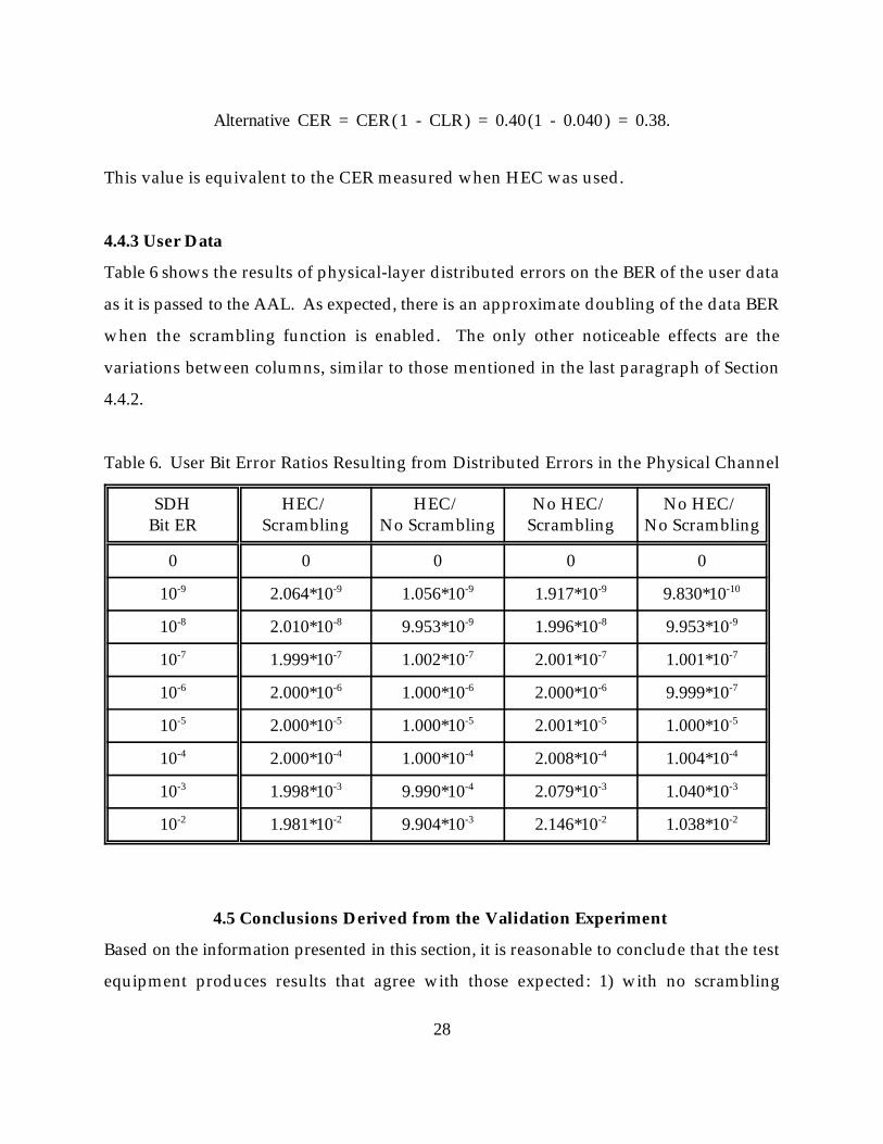
4.4.3 User Data

Table 6 shows the results of physical-layer distributed errors on the BER of the user data

as it is passed to the AAL. As expected, there is an approximate doubling of the data BER

when the scrambling function is enabled. The only other noticeable effects are the

variations between columns, similar to those mentioned in the last paragraph of Section

4.4.2.

Table 6. User Bit Error Ratios Resulting from Distributed Errors in the Physical Channel

SDH HEC/ HEC/ No HEC/ No HEC/Bit ER Scrambling No Scrambling Scrambling No Scrambling

0 0 0 0 0

10 2.064*10 1.056*10 1.917*10 9.830*10-9 -9 -9 -9 -10

10 2.010*10 9.953*10 1.996*10 9.953*10-8 -8 -9 -8 -9

10 1.999*10 1.002*10 2.001*10 1.001*10-7 -7 -7 -7 -7

10 2.000*10 1.000*10 2.000*10 9.999*10-6 -6 -6 -6 -7

10 2.000*10 1.000*10 2.001*10 1.000*10-5 -5 -5 -5 -5

10 2.000*10 1.000*10 2.008*10 1.004*10-4 -4 -4 -4 -4

10 1.998*10 9.990*10 2.079*10 1.040*10-3 -3 -4 -3 -3

10 1.981*10 9.904*10 2.146*10 1.038*10-2 -2 -3 -2 -2

4.5 Conclusions Derived from the Validation Experiment

Based on the information presented in this section, it is reasonable to conclude that the test

equipment produces results that agree with those expected: 1) with no scrambling

29

function, the user BER was equivalent to the physical-layer BER; 2) the scrambling function

doubles the user BER; 3) the CER was approximately 384 times the physical-layer BER,

4) CLR was 40 times the physical-layer BER; and 5) the HEC function eliminated cell losses

until the BER was 10 . These results provide some confidence in the application of the test-2

equipment to situations where Poisson errors are not the norm, and “bursty” errors

dominate.

An important conclusion of this experiment is the is the need to investigate error

distributions other than Poisson. The importance of this is evident by observing the ATM-

layer performance results attained when the physical-layer Poisson error model is used.

For example since the G.826 objectives are just met at a BER of 10 , (see Table 4), the-9

corresponding I.356 parameters are (by averaging across relevant columns for 10 SDH-9

BER in Table 5):

CER 3.9 * 10-7

CLR (with HEC) 0

CLR (without HEC) 4.7 * 10-8

SECBR 0

It would be misleading to provide this information to application developers because it

indicates that they would never have to deal with lost cells or severely errored cell blocks.

Since none of these parameters actually equal zero, and because some events will cause cell

loss and severely errored cell blocks, it is important to consider a more complex model of

physical-layer channel conditions. A model that contains three channel conditions (e.g.,

error-free operation, slightly errored operation, and severely errored operation) would be

required to provide a minimally useful description of the performance characteristics of

a real ATM network. As stated in Section 3 of this report, four channel conditions were

used in the experiments discussed in Sections 5 and 7.

30

5. RELATING PHYSICAL- AND ATM-LAYER PERFORMANCE USING THE BNE

This section describes results using the BNE to study the effects of transmission

impairments on ATM-layer cell transfer performance. In these experiments, empirical data

about ATM-layer performance was collected when the physical-layer performance just met

the objectives of Recommendation G.826. The Phase 1 emulator configuration shown in

Figure 2 and the physical-layer error model described in Section 3.3 were used.

To conduct relevant experiments, the error generator in the BNE must be able to generate

physical-layer conditions that are very close to the (G.826) physical-layer performance

objectives. This is done by assigning appropriate error ratios and transition probabilities

in the error model. The first step is to establish criteria regarding the types of errors to be

injected. Among the characteristics to be considered are the burstiness of the errors and

the type of “severe” degradation that should be injected. Below, we consider two error

scenarios and two severe error conditions.

In the first error scenario, the errored seconds (ES’s) are distributed as widely as possible.

With the ESR objective of 0.160, an error of some sort would be encountered approximately

every sixth second. The physical-layer BER during those seconds is a combination of 10-5

and 10 . In the second scenario, the errored seconds are “clumped,” with an average of-7

10 consecutive errored seconds in every minute. The physical-layer BER during those

errored seconds is a combination of 10 and 10 . The severe error condition established-6 -8

is either a 625 µs (5 SONET/SDH frames) sync loss or an error ratio of 10 . The-2

combinations of these conditions create four case studies of ATM Performance, namely,

scattered ES with sync loss, clumped ES with sync loss, scattered ES with high BER, and

clumped ES with high BER..

Pcase 1 =

0.9968412 0.00232802 0.00083078 0.0

0.1731765 0.826451 0.0003725 0.0

0.9034 0.0 0.057 0.0396

1.0 0.0 0.0 0.0

For all cases, an empirical and iterative process was followed. That is, an initial10

transition probability matrix was calculated based on the desired error conditions and theinformation presented in Section 4. That matrix was then used to generate performancevalues, and those values used to refine the transition probability matrix. This iterativeprocess occurred until the G.826 performance values were within 10% of the objectives,without exceeding them. These values are reported with more precision than the resultsbecause they represent the exact values used in the ‘C’ code implementation.

31

5.1 Case 1: Scattered ES with Sync Loss

The states for case 1 were assigned as follows: state 1 = error free state; state 2 = 10 BER;-7

state 3 = 10 BER; and state 4 = sync loss. In order to create a scattered ES scenario that just-5

met G.826 performance objectives, the following transition probability matrix was10

required:

The performance parameter values for this case are shown in Table 7. The experiment

duration was 40 hours, and ATM user cells totally filled the SONET payload space. Note

that two CLR values were computed. As defined in Recommendation I.356 (see Section

2.2), a cell loss occurring in a severely errored cell block is not actually considered in the

computation of CLR. Because of the types of errors introduced and the efficiency of the

HEC, all cell losses occurred only in severely errored cell blocks. Therefore, the I.356 CLR

is 0.0. Since cells were actually being lost, a user-perceived CLR was calculated. This was

the CLR that a user might have perceived when comparing the cells injected into the

network to the cells delivered by the network; providing an indication of the number of

cells that are being lost (in this case, in severely errored cell blocks).

The BNE has the capability of performing experiments with both the SONET and SDH11

physical layer protocol. For these experiments, the SONET protocol was chosen.

32

Table 7. Performance Parameter Values for Case 1

G.826 Performance Parameter Values I.356 Performance Parameter Values

ESR 0.155 CER 4.2 * 10-6

SESR 0.00182 SECBR 1.34 * 10-6

BBER 0.000198 CLR (I.356) 0.0

CLR (perceived) 1.16 * 10-6

Also important to consider is the creation and result of the sync loss state used in case 1

and case 2. The sync loss was created through inverting the SONET frame word for11

several consecutive frames. SONET loses synchronization after two consecutive inverted

frame words, and resynchronizes after two valid frame words have been received. Given

this, the number of SONET frames “lost” is the same as the number of consecutive frames

in which the frame word was corrupted. During this emulated sync loss, all ATM cells

within the affected SONET frames are lost. Multiplying the number of affected SONET

frames by 44.15 (2340 payload bytes per STS-3c frame/53 bytes per ATM cell) gives the

number of ATM cells that were lost in the event. Because the receiving hardware has no

ability to determine the exact number of cells that were in the lost SONET frames, the

number of lost cells has to be estimated using the a priori information about sync-loss

duration and number of cells in a frame.

5.2 Case 2: Clumped ES with Sync Loss


state 3 = 10 BER; and state 4 = sync loss. In order to create a clumped ES scenario that just-6

met G.826 performance objectives, the following transition probability matrix was

required:

Pcase 2 =

0.99975075 0.0001795 0.00006975 0.0

0.0030953 0.9822713 0.0139429 0.0006905

0.0036053 0.1765714 0.8191428 0.0006805

0.95 0.0 0.0 0.05

Pcase 3 =

0.999751142 0.000179025 0.000069833 0.0

0.00309 0.9852841 0.0109929 0.000633

0.00359 0.1382342 0.8575428 0.000633

0.95 0.0 0.0 0.05

33


duration was 40 hours, and ATM user cells totally filled the SONET payload space. The

two CLR values are explained in Section 5.1.



ESR 0.158 CER 3.8 * 10-6

SESR 0.00193 SECBR 1.56 * 10-6

BBER 0.000189 CLR (I.356) 0.0


5.3 Case 3: Scattered ES with High BER


state 3 = 10 BER; and state 4 = 10 BER. In order to create a clumped ES scenario that just-6 -2


required:



two CLR values are explained in section 5.1. Because the severe error condition for both

Pcase 4 =

0.9971784 0.0022939 0.0005277 0.0

0.132978 0.846451 0.02 0.000571

0.414 0.5 0.05 0.036

0.95 0.0 0.0 0.05

34



ESR 0.160 CER 1.21 * 10-5

SESR 0.00180 SECBR 3.6 * 10-5

BBER 0.000196 CLR (I.356) 0.0


case 3 and case 4 is a 10 BER, all cells actually reach the ATM receiver; it is possible for-2

that component of the system to precisely determine the number of cells lost due to

physical-layer channel conditions. Therefore, the perceived CLRs calculated for these two

cases were observed rather than estimated, as they were for case 1 and case 2.

5.4 Case 4: Clumped ES with High BER


state 3 = 10 BER; and state 4 = 10 BER. In order to create a scattered ES scenario that just-5 -2


required:



need for two CLR values is explained in section 5.1.

5.5 Performance Comparisons

The results of the four physical-layer error scenarios (case 1 through case 4) are

summarized in Table 11. In all four scenarios, the physical-layer performance values are

As noted in previous sections, the values of CLR (I.356) is reported as zero because all12

lost user cells observed during the experiments occurred in severely errored cell blocks.

35



ESR 0.157 CER 2.5 * 10-5

SESR 0.00185 SECBR 3.7 * 10-5

BBER 0.000195 CLR (I.356) 0.0


Table 11. Range of Performance Parameter Values for Cases 1 Through 4


ESR 0.155 - 0.160 CER 3.8 * 10 - 2.5 * 10-6 -5

SESR 0.00180 - 0.00193 SECBR 1.34 * 10 - 3.7 * 10-6 -5

BBER 0.000189 - 0.000198 CLR (I.356) 0.0

CLR (perceived) 7.7 * 10 - 1.34 * 10-8 -6

within 10% of the G.826 objectives. In the ATM-layer performance parameter valus, all

parameters except CLR (I.356) had a significantly larger variation across the cases. For12

the CER, the variation across the four cases is more than a factor of 6 (case 4 to case 2). The

difference in the perceived CLR was even greater: almost a factor of 20 between case 3 and

case 2. Finally, there was more than a factor of 25 difference between the SECBR of case

1 and that of case 4.

These differences are primarily related to the type of severe error condition used for that

case. Those cases that used a sync loss had a higher perceived CLR and a lower CER than

those that used a 10 physical-layer BER for the severe error condition. This is explainable-2

when one considers the effect of the errors on the ATM cell stream. The sync loss caused

36

all ATM cells in the affected SONET/SDH frames to be lost (approximately 220 cells per

occurrence) with no errored cells. On the other hand, during a 10 BER period of 17 ms,-2

an average of only 11 cells were lost, but almost all remaining cells (about 6000) were

errored during that period. Further examination (not detailed here) shows that these

errored cells comprised between 65% and 85% of all errored cells in cases 3 and 4.

The primary conclusion based on these comparisons is that variations in the type and

distribution of errors in the physical layer can produce significantly different performance

parameter values at the ATM layer with very little change in the physical-layer

performance parameter values. This suggests the need for additional, more detailed

studies.

= SONET OC-3 on Single Mode Fiber

= ATM Switch

U.S. Department of CommerceBoulder Laboratories

EmulatorNetwork

Campus Network

The network provided ATM bearer services as part of an exchange carrier’s trial. The13

results reported here should not be construed as an evaluation of the carrier’s services,extant or planned.

37

Figure 5. Phase 1 network configuration.

6. USING THE BNE TO STUDY PERFORMANCE OF A PROTOTYPE ATM NETWORK

This section describes results of applying the BNE to study the ATM cell transfer

performance of a prototype ATM network. The initial phase of the trial consisted of six13

ATM switches, located in customer premises throughout a metropolitan area, connected

in a SONET ring architecture, while the second phase had a significantly different

architecture utilizing two ATM switches at central office (CO) facilities.

6.1 Network Trial: Initial Architecture

As previously mentioned, the initial phase

of the trial consisted of six ATM switches.

The switches were interconnected in the

configuration shown in Figure 5. At each

switch site, local experimenters could

access a connection appropriate for their

respective experiments. In most cases,

those connections were Ethernet, but also

included FDDI (Fiber Distributed Data

Interface), TAXI (Transparent

Asynchronous Transceiver Interface), video (digitally encoded and decoded by an

interface card within the switch), and SONET/STS-3c. ITS test equipment was connected

to the trial network via an STS-3c.

All logical connections through an ATM network are made using virtual connections.

Each ATM cell is assigned to a virtual connection that is identified by the combination of

38

the VPI (virtual path identifier) and the VCI (virtual channel identifier) in the header of the

ATM cell. There are two types of virtual connection: permanent (PVC) and switched

(SVC). For SVCs, every time data needs to be transferred between two terminals, a

connection is established (this is much the same as a voice circuit being set up every time

one user dials another on the public switched telephone network). PVCs are set up once,

and remain available until they are disabled by the ATM switch administrator. The

capabilities of the switches and terminal equipment used in the trial were such that all

logical connections were required to be made via PVCs. Each participant was assigned a

channel or suite of channels to send and receive data for their respective experiments. It

should be noted that even though the connections were not switched for the trial, all ATM

cells passing through the network still had to be switched from one channel to another.

The channels assigned to ITS are shown in Table 12. Odd-numbered channels between 211

and 222 were used for sending data and even-numbered channels were used for receiving.

This choice was somewhat arbitrary, as these connections were configured to be

symmetric. Data was sent on one channel through the indicated number of switches. At

that point, it was switched to the receive channel, and retraced its path back to its origin.

These channels were used to conduct CTD, CDV and CLR measurements (see Section 2.2).

Channels 230 and 231 were routed somewhat differently. The data for this channel entered

the network at the ITS site, passed once around the ring (as shown in Figure 5), and then

returned to the ITS site. These PVCs were used to test network utilization. Finally, PVC

225 was established to allow the testing described in Section 6.1.2.

6.1.1 Test Description for the Initial Phase of the Network Trial

Two types of tests were conducted to determine the feasibility of using the BNE to make

performance measurements of the prototype ATM network. One series of tests was used

to measure CTD, 2-point CDV, and CLR. The second series was used to determine

network utilization.

39

Table 12. Channels Assigned to ITS for Phase 1 of the Network Trial

Send Receive Number of Times Data Number of Switches Channel Channel Was Switched

211 212 1 1

213 214 3 2

215 216 5 3

217 218 7 4

219 220 9 5

221 222 11 6

225 225 3 2

230 231 8 6

6.1.1.1 CTD, CDV, and CLR Measurements

Each measurement of CTD, CDV and CLR was conducted over a 3-hour period and was

repeated for 42 different conditions. CLR was measured continually over the 3-hour

measurement period, but it was not possible to measure CTD and CDV in a continuous

manner. Instead, absolute cell transfer delay was measured for 4096 consecutive cells at

5-minute intervals. For each 4096 cell sample, five data points were noted: maximum,

minimum, mean, and mean plus or minus one sample standard deviation. Points from

consecutive samples can be plotted to provide an indication of how CTD varies with time.

Cell delay variation measurements used the same cells as the CTD measurement. An

initial delay (T0) is the delay of the first cell measured in the 3-hour test; CDV is presented

as the difference between that time and the absolute cell transfer delay of any other cell

measured. In total, CTD and CDV were measured for 147,456 cells during each 3-hour

measurement.

40

6.1.1.2 Network Utilization

The network utilization test determines the amount of the network’s resources used over

time. To accomplish this, a channel that traversed the ring of ATM switches was created

(230/231). ATM cells were transmitted by the test equipment at the maximum allowable

data rate of 149.76 Mbit/s, switched around the ring, and then returned to the point of

origin.

This experiment required consideration of the ATM cell loss priority (CLP) bit setting. The

CLP bit is used to provide a level of importance when cells must be discarded (e.g., during

network congestion). Cells with a CLP of one (CLP=1) are discarded before those with a

CLP of zero (CLP=0). For all user-to-user and maintenance traffic on the trial network,

CLP=0.

If a stream of CLP=1 cells is sent into a network, only those cells that can be passed without

requiring a CLP=0 cell to be dropped will emerge from the network. Injecting CLP=1 cells

at a rate equivalent to channel capacity ensures that all available cells through the network

will be utilized by either a CLP=0 user-to-user or maintenance cell or a CLP=1 cell from

the test instruments. When the CLP=1 cells emerge from the network, the utilization is

equivalent to the difference between the data rate of those emerging cells and the channel

capacity. This does not provide a link-by-link assessment of the network utilization, but

rather the utilization of the busiest link. Also, since this traffic went around the ring in one

direction only, it is only measuring traffic in that direction. The traffic could have been

looped back at the switch which closed the ring to reveal the loading of the busiest link in

the network.

The utilization data was collected continuously over the 24-hour period, and recorded at

5-minute intervals. This data is plotted to show utilization at various times of the day in

Figure C-15 of Appendix C.

41

6.1.2 Network Trial Results for the Initial Phase

Examples of the data collected on CTD and CDV are shown in Figure 6. (For a complete

set of graphical data from the experiments conducted during the initial phase of the

network trial, see Appendix C.) The data covers three configurations when the bit rate of

the ATM cells is 140 Mbit/s (approximately 330,000 cells per second). The configurations

are as follows: 1) the data is passed through a 6-meter loopback cable, 2) the data is

switched three times, and 3) the data is switched 11 times. For each of the three switch

configurations, there are two graphs: a plot of CDV and a plot of CTD. The CDV plot

shows the histogram of cell delay relative to the first cell (with a delay of T0). The CTD

plot shows CTD at 5-minute intervals, including mean (heavy line), plus and minus one

standard deviation (shaded area), maximum (top dashed line) and minimum (bottom

dashed line). From Figure 6 it is obvious that as the number of switches in a connection

increases, the average delay and the delay variation increase. The results available in

Appendix C also make it obvious that delay and delay variation increase as the data rate

increases.

6.2 Network Trial: Second Phase

Building on the knowledge gained in initial phase, the exchange carrier implemented a a

new architecture for the second phase of the trial. The architecture in this phase was

significantly different than that of the initial phase, in that it had only two switches housed

in CO facilities. All test participants were connected to one of these switches. The physical

configuration is shown in Figure 7a. Again, ITS was assigned channels for use in testing

the network. The logical configuration of the channels is shown in Figure 7b. There were

four logical paths for use in testing. Two were looped back at the first switch and two

were looped back at the second switch. At each loopback point, cells could loop back to

the same channel or switch to a second PVC.

42

Figure 6. Example cell delay variation and cell transfer delay measurement results.

43

Figure 7. Physical and logical configuration for the second trial network phase.

In SONET and SDH, network equipment timing clocks can be synchronized through14

a process called “slaving.” One piece of equipment is designated as a master for timingpurposes, and all other equipment derive their timing based on the signal from the master.The derived timers are referred to as “slaves.”

44

Much of the testing on the second phase network was the same as for the first phase,

including the CTD, CLR and CTD tests. In this configuration, however, we did not

perform utilization tests due to scheduling conflicts with the experiments of other

participants. Instead, a study was conducted on long-term measurement of CTD, and the

relationship between CTD and cell loss was studied. The results of the CTD and CDV

testing are in Appendix D; the test description and results of the other studies are

discussed below.

6.2.1 Long-term Measurement of CTD on The Second Phase of the Prototype Network

For the long-term measurement of CTD, two virtual channels were used. On PVC

214/215, cells were sent at a rate of 1 cell every 4.24 seconds (i.e., an average rate of 100

bit/s). The remaining ATM-layer capacity was filled with pseudorandom data sent on

channel 211. This amounted to an average of 353,207.31 cells/s (i.e., 149.7599 Mbit/s). The

individual delays of 4096 consecutive cells on channel 214/215 were recorded. The overall

time of the measurement was approximately 4 hours 49 minutes and 23 seconds, and the

results are shown in Figure 8.

There was a fairly rapid increase in delay for approximately the first 100 cells, and then

a more moderate increase for the next 700 cells. The delay reaches a relatively stable level,

and then plummets. The increasing pattern recurs, with a final stabilization at about

10 msec of delay. We hypothesize that the increasing delay is due to a difference in

SONET transmission timing. In particular, the steep part of the curve is due to the

difference between the SONET timing clock in the host switch and the test instruments,

and the moderate slope is due to a SONET timing clock difference between the two

switches. When these results were presented to the exchange carrier, they noted that the

SONET clocks in their switches had not yet been slaved together. Once the clocks were14

0

2

4

6

8

10

12

0 500 1000 1500 2000 2500 3000 3500 4000 4500

Cells on VC 214/215

45

Figure 8. Long-term cell delay measurement on the Phase 2 network.

synchronized, and the test was conducted again, there was no longer a two-stage increase

in delay, only a single stage (due to the difference between the SONET transmission clock

in the test instrument and that in the host switch).

When the delay seemed stable, a small CLR was observed. Further examination of the

data revealed that the delay was not actually stable during this period; rather, the delay

varied in a sawtooth pattern of a magnitude too small to see clearly on Figure 8. This

phenomenon, also due to a difference in clocks, is investigated further in Section 6.2.2. The

sudden decrease in delay shown in the graph is due to a catastrophic buffer flush. It is

unknown why this occurred, and the effect was not observed again.

46

Figure 9. Evidence of cell loss due to buffer overflow.

6.2.2 Relating CTD and Cell Loss during the Second Phase of the Prototype Network

The need to study the relationship between CTD and cell loss was indicated by the results

of the long-term delay measurements. This phenomenon was also investigated using two

virtual channels. In this case, timing information was sent on PVC 212/213 at a rate of

37.44 Mbit/s (i.e., an average of 88,301.89 cells/s, or ¼ of channel capacity). The remaining

channel capacity, 112.32 Mbit/s (i.e., 264,905.66 cells/s), was filled with pseudorandom

data on PVC 210. The individual delays and interarrival times of 4096 consecutive cells

on PVC 212/213 were measured. The overall time of the measurement was approximately

46 ms, and the results are shown in Figure 9.

The top trace on the graph represents the individual delays for the 4096 cells, and the

bottom trace represents the interarrival times for the same cells. The delay increases

slowly for approximately 3500 cells. This is due to a clocking difference between the ATM

In theory, the problems resulting in a difference in clock speeds could have been15

corrected by slaving the clock of the test instrument to that of the host switch, or vice versa.There was not sufficient time in the trial to enable testing of this theory.

47

cell generator and the host switch. The slope of the graph indicates that there is

approximately 3400 bit/s more than the host switch can properly process (i.e., the ATM

cell generator is sending data slightly faster than the switch can process it). As more data

arrives than the switch can process, it is forced to put the cells into a buffer. As the buffer

approaches its limit, eventually a cell does not exit the buffer in time for the next arriving

cell to be added to the queue. At this point, the buffer overflows, and a cell is lost. As

evidenced by the slow rate of increase in CTD, the discarded cell would be rejected

because only one or two of its bits will not fit into the buffer. By the time the remainder

of the buffer bits are reclaimed from the discarded cell, and another cell exits to be

processed, there is a net reduction in the delay of approximately 2.7 µs, the time it would

have taken to send the lost cell if it had not been lost. This event is indicated in Figure 9.

The interarrival time measurements corroborate this conclusion. There is a single

interarrival time that is approximately double the normal interarrival time, less the 2.7 µs

that the overall delay was reduced. Since the cells were injected into the network with an

accuracy of ± 1.35 µs, this increase cannot be due to an injection error. Likewise, since

delay decreased, there should have been a corresponding decrease in the interarrival time

if no cells were lost. Thus, we concluded that the single increase in the interarrival time

was due to a cell loss.15

6.3 Discussion and Conclusions

There are several observations that can be made based on the data collected. First, for

moderate network loading and a small number of switches, there should be little

performance degradation perceivable to a user. As the number of switches and the

network loading increase, however, this could change. As loading increases, and traffic

48

from multiple sources is multiplexed together, the buffers in the switches will fill and

empty. As the buffers fill, there will be an increase in delay. As buffers empty, delay will

decrease. Terminal equipment will have to buffer enough data to provide continuing

output when cells are delayed more than normal (as the buffers fill), yet provide enough

spare buffering capacity to hold the cells that arrive early (as the buffers empty). In order

to ensure there will be no overflow or underflow, the buffers on the terminal equipment

would have to be as large as the sum of the buffers on all of the switches passed through

by the channel (for a full bandwidth data stream). As the probability of all switch buffers

filling and emptying at the same time is very small, it would be extremely rare that this

much buffering would be necessary. Also, as ATM networks are deployed, traffic flow

mechanisms will be implemented and the potential delay variation should moderate. This

will help reduce the required size of buffers in the terminal equipment.

In addition to CDV, CTD could be an important issue as ATM networks are deployed.

During the test, delays of as much as 3.3 ms/switch was observed. This delay will

accumulate as the cell passes through the network, and, for a voice connection, could

become large enough to cause customer complaints. This is especially true when the

switching delays are coupled with the time that it takes to fill a cell with speech

(approximately 6 ms for audio digitized at 64 kbit/s to fill an ATM cell).

Based on the observed data, it can be concluded that the BNE can be successfully used to

measure the performance of live ATM networks. In addition, this set of measurements has

shown that performance measures can be used by network providers to determine and

resolve network problems. The testing also revealed that some sources of ATM

performance degradation are not intuitively predictable (e.g., SONET clocking differences

leading to ATM cell loss), providing validation for the position of not specifying error

cause when setting objectives for I.356 performance measurement parameters. Finally,

performance degradations that occur can and will have an impact on user applications.

Though some of the scenes were from other sources, including entertainment video,16

many of them were from American National Standard T1.801.01.

49

7. RELATING PHYSICAL-LAYER PERFORMANCE TO VIDEO QUALITY WITH THE BNE

Of ultimate interest in the study of performance interactions in B-ISDN is the impact that

errors in the various protocol layers have on application performance. In this Section, the

relationship between physical-layer impairments and video quality is explored. Video is

an application that is likely to make extensive use of B-ISDN ATM, especially its

multiplexing capabilities. (B-ISDNs will be used for distribution of entertainment video,

video conferencing and video telephony.) The BNE provides essential capabilities to

extend the performance experiments of Section 5 (impact of transmission impairments on

ATM cell transfer performance) to the application layer.

7.1 Experiment Description

For the experiment, a 30-minute test tape was created. Several scenes were selected for

inclusion on this tape in order to cover a full range of spatial and temporal resolution

requirements. [14] The temporal variation of the video scenes ranged from none in still16

images to significant amounts of action and scene cuts in entertainment video. The spatial

resolution of the scenes ranged from low-resolution “head and shoulders” video to highly

detailed scenes of flower gardens and landscapes. The video test tape was recorded in

component format (Y, R-Y, B-Y) from scenes previously recorded in that format. During

a test, the signal was converted to NTSC, digitally encoded, and then injected into the BNE

as shown in Figure 3. The network emulator introduced impairments, and then returned

the signal to the codec, where it was decoded into NTSC, converted to component format,

and recorded on tape.

For this experiment, two video-coding schemes at three data rates were examined. The

first coding scheme examined was ITU-T H.261 [15], a discrete cosine transform (DCT)-

The intent was not to examine impairments introduced by various coders, only those17

additional impairments that might be introduced through the use of an ATM network.Therefore, any comparisons in performance were between coded video passed through theATM network and the same coded video passed through a null network (i.e., loopback).

50

based scheme, at data rates of 1.536 Mbit/s and 384 kbit/s. The second was a proprietary

scheme, based on differential pulse code modulation (DPCM), at a data rate of

44.736 Mbit/s. This combination of coding schemes and data rates was chosen because it

provides three distinct levels of quality. The DPCM system provides a very high level of

quality, each of the 60 fields/second is fully coded, and the minimal amount of

compression (approximately 4:1), ensures little spatial detail will be lost. The H.261

system, because it can operate at any data rate that is a multiple of 64 kbit/s, can provide

a wide range of quality levels. At 1.536 Mbit/s, (approximately 100:1 compression) frame

repetition is limited to periods of high temporal activity, and detail is quite high in periods

of low motion. When the data rate is reduced to 384 kbit/s (approximately 400:1

compression), frame repetition increases and detail decreases, both of which reduce the

overall quality of the video.

Once the video was digitally coded, it was subjected to three different network conditions.

The first was a null error condition, useful for determining if the ATM multiplexing

process intrinsically causes some degradation in the video service. After that, the video

was passed through the network being subjected to the errored conditions described in

Sections 5.3 and 5.4 (case 3 and case 4, respectively). This was done to help determine the

impact that different error distributions have on application performance.

Once the video had been passed through the ATM network and recorded, the tapes were

examined to determine the extent of any impairments introduced by the network or the

BNE. This examination was performed visually in both real-time and on a field-by-field17

basis. The real-time examination allowed for the discovery of major, perceivable

In the case of NTSC video, a field is represented by the odd or even raster lines of an18

interlaced video frame. There are 60 fields per second (i.e., 30 frames per second).

51

impairments, while the field-by-field analysis provided more detail about the exact18

number of fields containing errored video. Because of the exploratory nature of this

experiment we decided visual frame-by-frame analysis was preferable to a subjective test,

which can be very time-consuming and expensive. In addition, reporting video errors in

terms of ES, SES and BBER assists in the comparison of application-layer errors to

physical-layer errors. (A “block” was considered to be one field of video for this

experiment.) Subjective testing may be used for future experiments, and, as they mature,

perception-based objective measures may be applied to this type of data [16].

7.2 Results

There seemed to be no inherent degradation caused by multiplexing the digital video

signal onto an ATM network. In all three cases, the signal multiplexed onto the ATM

network was indistinguishable from the same signal passed through a null network

(loopback). Also apparent was how the two coding schemes responded to errors in the

ommunication channel. The DCT system had better characteristics under moderate error

conditions, but the DPCM system recovered from error effects much faster than the DCT

system.

The DPCM system seemed to have no capacity for error detection and correction. When

a single bit error occurred, a domino effect was started in the video field being transmitted.

When one of these fields was examined, the point where the original error occurred was

apparent (e.g., in the checkerboard pattern of the finish line in the image shown in Figure

10). From the point of origin, the error propagates down and to the right until it

encounters the synch pulse. At that point, the remainder of the field dissolves into

multicolored “confetti.” Even though the effect of an error can be quite severe to a field,

recovery is quick because the DPCM algorithm resynchronizes at the beginning of the next

These parameters were chosen for comparison with physical-layer phenomena. While19

it is intuitive that there will be some relationship between these performance parametersand subjective opinion, the specific relationship between these parameters and subjectiveopinion requires further study.

For video, this corresponds to 59.94 blocks/s. There are 746,346 bits/block for the20

DPCM system and 25,625 bits/block for the H.261 system. This is in contrast to thephysical layer, where there are 8,000 blocks/s and there are 19,440 bits/block.

52

field. In real-time the error is perceived as a momentary flash in the signal. As a single,

isolated event, a viewer would not find this error response annoying. However, when

they come in a burst of several errored fields per second, a strobe-like effect is produced

that viewers would subjectively classify as “very annoying.”

The primary error-related problem that was observed in the DCT system was the length

of time taken to recover from errors. The system seemed to be fairly robust under bit error

ratios of 10 or less, but error-related video impairments began appearing at higher error-5

ratios. The first type of error observed was errored blocks [17], where a square area of the

image changes color, or otherwise becomes disassociated from the rest of the image. The

codec took up to 15 seconds to recover from an errored block. The next level of

impairment is that of the image freezing. This video “freeze” was observed to last up to

30 seconds, with full recovery taking up to 28 additional seconds. Figure 11 shows how

the video looks during recovery.

It is desirable to determine a means of comparing these two error responses with the error

information available on physical-layer performance. To facilitate this comparison, it

would be useful to define parameters for the video signal that are similar to the physical-

layer performance parameters (BBER, ESR, SESR). The definitions for the ESR for the19

video is fairly straightforward: the ratio of errored seconds to total seconds in the

measurement interval. For the other two parameters, it is necessary to define a block. For

the video, a block was considered to be one field of video. With this definition, the20

53

Figure 10. Example of error occurring during transmission of DPCM-encoded video.

Figure 11. Example of video from DCT-based codec recovering from a “freeze.”

54

background block error ratio will be the same as that given for the physical layer in Section

2.1.

Because of the differences in the error responses of the two video systems, it seems that

different definitions for an SES must be considered. In the case of the DCT system, there

is a threshold at which the video freezes. This makes an obvious candidate for the

definition of a severelyerrored second for that system. Table 13 shows performance values

of the DCT-coded video based on this definition of a severely errored second. The “# of

events” category in the table indicates the number of groups of consecutive errored

seconds during the test.

For the DPCM system, every field is fully transmitted, and therefore there is no

corresponding event to indicate that the errors are severe. For the DPCM system, a

threshold must be defined that indicates the number of errored fields allowable before an

errored second becomes a severely errored second. The value of this threshold will affect

the value of both the SESR and the BBER. To demonstrate this effect, performance

parameter values for SESR and BBER are presented as a function of this threshold for both

case 3 and case 4. The effect of the errored field threshold on SESR is shown in Figure 12

and the effect on BBER is shown in Figure 13. Subjective testing is required to determine

Table 13. Performance Parameter Values for the DCT-Based Video Codec

Case Video Bit Rate # of Events ESR SESR BBER*

3384 kbit/s 6 0.026 0.0088 0.0154

1.544 Mbit/s 7 0.090 0.066 0.024

4384 kbit/s 11 0.066 0.0176 0.044

1.544 Mbit/s 9 0.084 0.062 0.021 See Section 5.3 for a description of case 3 and Section 5.4 for a description of case 4.*

55

Figure 12. SESR as a function of the errored field threshold for an SES.

Figure 13. BBER as a function of the errored field threshold for an SES.

56

the exact threshold at which enough fields become errored to constitute a severely errored

second of video. It is expected that this value will be somewhere between 10 and 20

errored fields. This would indicate that the SESR would range between 6 * 10 and 4 * 10-4 -2

and the BBER would range between 5 * 10 and 1 * 10 . The ESR for the DPCM codec is-3 -2

0.115 for case 3 and 0.130 for case 4. The number of groups of errored seconds (# of events)

is 143 for case 3 and 133 for case 4.

7.3 Discussion of Results

One of the most interesting results of this experiment is the wide variety of application

performance that can result from a single set of physical-layer error conditions. For the

same physical-layer error conditions, parameters varied from as little as a factor of two to

as much as two orders of magnitude, depending on the application (video-coding scheme

and bit rates in this case) and definition of the parameters (specifically, the SESR

threshold). This is evidence that there is no simple mathematical relationship between the

performance of the physical layer and that of all applications.

This is further evidenced by looking at the number of groups of errored seconds. The DCT

system had relatively few error events (between 6 and 11) of a long duration while the

DPCM system had 115 to 130 events of a much shorter duration. If the physical-layer error

pattern were to be examined, it would be much closer to the patterns observed in the

DPCM codec than those of the DCT codec. This provides evidence of two different

dependencies for physical layer applications: 1) the relation of the physical-layer and

application error patterns, and 2) the application error recovery time. The first

dependency is generally a function of the application’s ability to detect and/or correct

errors. The second is a function of the handshaking required for the systems to fully

resynchronize communications after an error occurs.

57

In the case of these applications, there seems to be a direct trade-off between error

frequency and recovery time. As B-ISDNs are implemented, users will be able to request

a specific ATM performance class from those that the networks support. While many

details have yet to be standardized, the basic premise is that a user will be willing to pay

for better performance, if it is required to meet application needs. The precise levels of

network performance required for the various applications that users will have is still

under study.

58

8. SUMMARY

This report has explored performance issues arising in the standardization and commercial

deployment of B-ISDN. The exploration included the comparison of ATM-layer cell

transfer performance under a variety of physical-layer error conditions, the performance

assessment of a prototype network, and an initial investigation of the impact of physical-

and ATM-layer transmission impairments on video quality. Relevant performance

measurement standards, specifically ITU-T Recommendations G.826 and I.356, were used

to conduct the experiments.

The exploration into performance interactions began with the development of a B-ISDN

network emulator. Phase 1 of the BNE had no external interfaces, and all emulations were

performed within the box. Phase 2 added external interfaces so that live data from

applications could be incorporated into the experiments. The development of a four-state

Markov model to generate network impairments was presented, along with a simple

validation.

Once the BNE capabilities were validated, the emulator was used to explore the

performance interactions between the physical layer and the ATM layer. Four “cases”

were created based on the four-state Markov model. The cases were based on

combinations of two types of error patterns (“scattered” and “clumped” errored seconds)

and two types of severe impairment conditions (sync loss and 10 bit error ratio). The-2

performance values were compared, and significantly different ATM-layer performance

parameter values were observed for different distributions of physical-layer errors.

The measurement capabilities of the BNE were applied to two developmental phases of

a prototype ATM network. An overall description of the initial and second phases of the

trial network was provided along with measurement results. Results showed that the BNE

59

can be used to measure performance of a live ATM network; physical topology affects the

values of performance parameters; small differences in physical layer timing can have an

impact on performance; performance measurements can be used to diagnose

implementation differences and network problems; and that performance at the physical

and ATM layers will impact application performance.

Finally, physical-layer/application-layer performance interactions were explored using

the BNE and video, an application expected to be common for B-ISDNs. Two different

video-coding schemes, DCT and DPCM, were used at three different bit rates (44.736

Mbit/s for the DPCM system and 1.536 Mbit/s and 384 kbit/s for the DCT system). These

two systems had very different behavior characteristics when the physical-layer stream

was subjected to errors. The DCT system was robust under moderate errors, but had a

long recovery time once affected by a higher bit error ratio. The DPCM system was

susceptible to losing a field of video based on a single physical-layer bit error, but

recovered fully upon transmission of the next field. This indicated that there may be some

application-layer performance trade-offs, even though the application designers may have

no control over physical-layer errors.

We have seen evidence that, in the future, testing over a selection of applications will be

required to provide a representative sample of performance relationships. Some examples

of applications include voice and video, using a variety of coding schemes and for a

variety of uses. Also important would be the study of data and image transfer across a B-

ISDN. The BNE could be useful in such studies. Capabilities could be added to the BNE

to improve the range of studies that can be conducted. Primary among these is a

controlled switching environment. This would enable the addition of controlled delay and

delay variation, as well as the ability to study the effects of network congestion on

performance of both ATM and applications.

60

[1] Alliance for Telecommunications industry Solutions, Committee T1 Secretariat,“Committee T1 - Telecommunications, Year 2000 Strategic Plan (Revised 1995),” in“Defining the Telecommunications Network of the Future.”

[2] Vice President Gore, “Global Information Infrastructure,” before the InternationalTelecommunications Union (ITU) Conference, Buenos Aires, March 21, 1994 in“National Information Infrastructure Progress Report, September 1993-1994,”Secretary of Commerce Ronald H. Brown, Chairman, Information InfrastructureTask Force, Sep. 9, 1994.

[3] ISO/IEC/ITU, “International Seminar on the Standards Aspects of the GlobalInformation Infrastructure (GII),” Geneva, Jan. 24-26, 1995.

[4] J. Richters and C. Dvorak, “A framework for defining the quality of communicationservices,” IEEE Communications Magazine, Vol. 26, No. 10, pp 17-23, Oct. 1988.

[5] N. Seitz, S. Wolf, S. Voran, and R. Bloomfield, “User-oriented measures oftelecommunication quality,” IEEE Communications Magazine, Vol. 32, No. 1, pp 56-66, Jan. 1994.

[6] ITU-T Recommendation I.350, “General Aspects of Quality of Service and NetworkPerformance in Digital Networks, Including ISDNs,” Geneva, 1993.

[7] ITU-T Recommendation G.826, “Error Performance Parameters and Objectives forInternational, Constant Bit Rate Digital Paths at or above the Primary Rate,”Geneva, 1993.

[8] ANSI, Inc,. “American National Standard for Telecommunications - NetworkPerformance Parameters and Objectives for Dedicated Digital Services - SONET BitRates,” ANSI T1.514-1995, New York, 1995.

[9] ITU-T Recommendation I.356, “B-ISDN ATM Layer Cell Transfer Performance,”Geneva, 1993.

[10] ANSI, Inc., “American National Standard for Telecommunications - B-ISDN ATMLayer Cell Transfer - Performance Parameters,” ANSI T1.511-1994, New York, 1994.

[11] J. Watkinson, The Art of Digital Video, London: Focal Press, 1990, pp. 28-30.

[12] Noorchashm, M.R., Relationship Between ATM Layer NP and the NP of the PhysicalLayer, Standards Contribution T1A1.3/92-091, October 1992.

9. REFERENCES

61

[13] ITU-T Recommendation I.432, “B-ISDN User-Network Interface - Physical LayerSpecification,” Geneva, 1993.

[14] ANSI, Inc., “American National Standard for Telecommunications - DigitalTransport of Video Teleconferencing/Video Telephony Signals - Video Test Scenesfor Subjective and Objective Performance Assessment,” ANSI T1.801.01-1995, NewYork, 1995.

[15] ITU-T Recommendation H.261, “Video Codec for Audiovisual Services at p x 64kbit/s,” Geneva, 1993.

[16] ANSI, Inc., “American National Standard for Telecommunications - DigitalTransport of One-Way Video Signals - Parameters for Objective PerformanceAssessment,” ANSI T1.801.03-1996, ANSI, Inc., New York, 1996.

[17] ANSI, Inc., “American National Standard for Telecommunications - DigitalTransport of One-Way Video Signals - Performance Terms, Definition, andExamples,” ANSI T1.801.02-1995, ANSI, Inc., New York, 1995.

62


63

APPENDIX A. ACRONYMS AND ABBREVIATIONS

AAL ATM adaptation layerANSI American National Standards InstituteATM asynchronous transfer modeBBER background block error ratioBER bit error ratioB-ISDN broadband ISDNbit/s bit(s) per secondBNE B-ISDN network emulatorCB cell blockCCITT International Telephone and Telegraph Consultative CommitteeCDV cell delay variationCER cell error ratioCES circuit emulation serviceCL cell lossCLP cell loss priority (bit in ATM cell header)CLR cell loss ratioCMR cell misinsertion rateCO central officeCODEC coder/decoderCRC cyclic redundancy checkCS convergence sublayerCSU channel service unitCTD cell transfer delayDCT discrete cosine transform (coding technology)DPCM digital pulse code modulationDS digital service DS-1 digital service level 1, 1.536 Mbit/sDS-3 digital service level 3, 44.736 Mbit/sDSU digital service unitER error ratioESR errored second ratioFCC Federal Communication CommissionFDDI fiber distributed data interfaceGFC generic flow control (field in ATM cell header)GP-IB general purpose instrumentation bus (IEEE-488)HEC header error control (field in ATM cell header)ISDN integrated services digital networkITS Institute for Telecommunication Sciences (part of NTIA)ITU International Telecommunication Union

64

ITU-T Telecommunication Standardization Sector of the ITUJPEG Joint Picture Experts Groupkbit/s kilobit(s) per second (1,000 bits per second)LM layer managementMbit/s megabit(s) per second (1,000,000 bits per second)MHz MegaHertzms millisecondN-ISDN narrowband ISDNNIU-F North American ISDN User’s ForumNNI network-node interfacensec nanosecondsNTIA National Telecommunications and Information AdministrationNTSC National Television System CommitteeOAM operation, administration and maintenanceOC optical carrierOSI Open Systems InterconnectionPL physical layerPM physical mediumPT payload type (field in ATM cell header)PUC Public Utilities CommissionPVC permanent virtual connectionSAR segmentation and reassemblySDH synchronous digital hierarchySECBR severely errored cell block ratioSES severely errored secondSESR severely errored second ratioSMA service module A (a ¼” threaded coaxial connector)SONET synchronous optical networkSTM synchronous transfer modeSVC switched virtual connectionTAXI transparent asynchronous transceiver interfaceTC transmission convergenceTOH transport overheadUNI user network interfaceusec microsecondVCI virtual channel identifier (field in ATM cell header)VPI virtual path identifier (field in ATM cell header)VXI A standard, open bus architecture that is the successor to the VME busXOR exclusive OR (logical operation)

SONET signals are also referred to with the label OC (for optical carrier). STS is1

generally used with electrical signals while OC is used with optical signals. For simplicity,STS has been used throughout this report.

65

APPENDIX B. OVERVIEW OF B-ISDN

The ITU-T (formerly CCITT) began work on B-ISDN standards during its 1984-1988 study

period. These standards outlined a system that would be a significant departure from any

previous telecommunications system. The system would be built on a foundation that

ITU-T dubbed the synchronous digital hierarchy (SDH) and the asynchronous transfer

mode (ATM). The SDH and ATM standards defined an optical fiber-based network with

channels operating at rates of multiples of 155.520 Mbit/s. U.S. standards bodies

developed the synchronous optical network (SONET) standard, which is similar to the

SDH system. Details of the SONET and SDH protocols are discussed in Section B.1.

The ITU-T continued to work on the development of B-ISDN Recommendations and, in

1991, adopted a protocol reference model for use in B-ISDN, Recommendation I.321. This

protocol reference model is shown in Figure B-1. The protocol reference model is similar

in concept to the OSI protocol stack, however, there are some differences. For example, the

divisions between the layers of the B-ISDN model do not correspond exactly to the levels

of functionality in the OSI model (e.g., some B-ISDN protocol layers are divided up into

sub-layers). The sub-layers and their respective functionalities are shown in Table B-1.

The ATM and AAL protocols are discussed in sections B.2 and B.3, respectively.

B.1 SONET/SDH Protocol

SONET and SDH were developed to provide high-speed reliable transport of digital

signals. During the development process, work was conducted in both the U.S. national

standards committees and the ITU. Table B-2 shows the data rates for a variety of SONET

and SDH channels. SONET channels are refered to with the label STS (for synchronous1

66

Figure B-1. B-ISDN protocol reference model.

transport signal) followed by the multiple of the 51.84 Mbit/s base rate that the channel

carries (e.g, STS-3=51.84 Mbit/s�3=155.520 Mbit/s). SDH channels are referred to with the

label STM followed by the multiple of the 155.520 Mbit/s base rate that the channel carries.

The SONET STS-1 stream is divided into 810-byte frames. This is generally depicted as

a block of information consisting of nine rows of 90 bytes each. (Figure B-2a.) The first

three bytes of each row (i.e., the first three columns of the frame) are transport overhead

information. In addition to this fixed overhead, there is a floating overhead component

that occupies one column of the payload field. This is path overhead. The transport

overhead is used to differing degrees by every device in the network, while the path

overhead is only used when the data in the frame is decoded.

67

Table B-1. Functions of the B-ISDN in Relation to the Protocol Reference Model*

Function Layer

LM

Higher Layer Functions Higher Layers

Convergence CSAAL

Segmentation and reassembly SAR

Generic flow controlCell header generation/extractionCell VPI/VCI translationCell multiplex and demultiplex

ATM

Cell rate decouplingHEC sequence generation/verificationCell delineation TCTransmission frame adaptationTransmission frame generation/recovery

PL

Bit timingPhysical medium

PM

Key:*

AAL ATM Adaptation Layer SAR Segmentation and ReassemblyATM Asynchronous Transfer Mode SublayerCS Convergence Sublayer TC Transmission ConvergenceLM Layer Management Sublayer PL Physical Layer VCI Virtual Channel IdentifierPM Physical Medium Sublayer VPI Virtual Path Identifier

Table B-2. SDH and SONET Channel Rates

Channel Rate (Mbit/s) SDH Level SONET Level

51.840 <not used> STS-1

155.520 STM-1 STS-3

622.080 STM-4 STS-12

1244.160 <not used> STS-24

2488.320 STM-16 STS-48

68

To form higher rate channels, these frames are multiplexed together using byte

interleaving. A 155.52 Mbit/s STS-3 has three of these frames interleaved as shown in

Figure B-2b. Note that all of the overhead information is included in the interleaving, as

well. In the 2430 byte STS-3 frame, there is 108 bytes of overhead information. This is

somewhat different from the overhead structure of an STM-1 frame of the same rate. In

the 155.52 Mbit/s STM-1 frame, there is only one column of path overhead floating in the

payload space as opposed to the three columns in an STS-3. The framing structure of

STM-1 is shown in Figure B-2c.

Note that the number of bytes of overhead in STM-1 is 18 bytes less than that of STS-3. In

order to alleviate this difference and improve the interworking between the international

and national standards, the U.S. national committees adopted a process called

concatenation. In concatenation, the payloads of the STS-1 streams are combined under

one set of path overhead bytes. This essentially equalizes the overhead with that agreed

upon in the international standards bodies. Channels that use a combined path overhead

are denoted by using a ‘c’ with the channel label. For example, the STS equivalent of STM-

1 is called STS-3c. By concatenating the payloads of the three STS-1s, the ability to

demultiplex the channel from an STS-3c to three STS-1s is lost.

There remain some differences in nomenclature and usage of the overhead between STM-1

and STS-3c, but since the aggregate data rate and the amount of overhead are equal

between the two systems, it is possible to achieve interworking between the U.S. standard

protocols and the international standard protocols.

B.2 ATM Cell Structure

In B-ISDN, the SONET or SDH frames are used to transport smaller chunks of data as

ATM cells. The ATM cells are asynchronous because they do not occupy a

fixedspacewithin the payload of the physical-layer frame. Within the physical-layer

69

Figure B-2. Framing structure for SONET and SDH frames.

70

payload, ATM cells can start and end at any point, as long as all cells in the payload space

are adjacent. ATM cells can even be split between two physical-layer frames, as long as

the bytes of the ATM cell are contiguous amongst the two payloads.

An ATM cell is 53 bytes long. The first 5 bytes, the header, are overhead. The remaining

48 bytes are cell payload. There are two different formats for an ATM header. One for the

user-network interface (UNI) and one for the interfaces between network nodes (NNI).

The format of an ATM UNI cell is shown in Figure B-3. The only difference between a

UNI and an NNI ATM cell is that the first 4 bits in an NNI cell are used for an enlarged

virtual path identifier (VPI) rather than for generic flow control (GFC).

In the cell shown in Figure B-3, the VPI and VCI (virtual channel identifier) bits combine

to form an “address” for the cell. This field helps ATM switches route the cell to the proper

destination. The payload type bits indicate whether the cell contains user data, operations,

administration and maintenance data; or resource management data. The cell loss priority

(CLP) bit is used to indicate the cells that should be discarded first in the case of network

congestion (i.e., when cells are entering queues to be transferred faster than the network

elements can transmit them). If the bit is set to one, the cell should be discarded before

discarding cells with a CLP of zero. The header error control field contains a cyclic

redundancy check (CRC) that can detect multiple bit errors in the header, and correct a

single bit error in the header. (See Section B.4 for more information on how the HEC is

generated and used.) The uses of the GFC field are currently under study by the national

and international standards bodies.

The ATM protocols provide few guarantees that a user’s data will arrive at its destination

intact. In fact, the only integrity guarantee is that cells will exit the network in the order

that they were inserted. Notably, ATM does not 1) request retransmission of lost or errored

cells, 2) guarantee that all cells will be delivered or that all cells delivered belong to that

BitByte12345678

1

2

3

4

5

6

to

53

GFC VPI

VCI

VPI VCI

VCI

HEC

Payload

PT CLP

GFC Generic Flow ControlVPI Virtual Path IdentifierVCI Virtual Channel IdentifierPT Payload TypeCLP Cell Loss PriorityHEC Header Error Control

71

Figure B-3. ATM UNI cell structure.

destination, or 3) guarantee that cells

inserted at a constant rate will be

delivered at a constant rate.

Although this seems detrimental to the

use of ATM, a significantly higher

percentage of overhead would be

required to implement these features;

this would leave less room for user

data. Thus, a compromise has been

achieved with the current structure

between throughput efficiency and

accuracy of information transfer. It

allows applications that require the

high data rate achievable in B-ISDN

networks to utilize that rate without

the burdensome overhead that

additional checks require. It also does

not preclude application developers

from providing their own mechanism for these functions in the higher layer protocols.

These developers will be assisted by information that provides a picture of how these ATM

characteristics affect the performance of a given channel.

B.3 ATM Adaptation Layer

The ATM Adaptation Layer (AAL) segments blocks of user data for transmission by the

ATM layer, and reassembles blocks of user data that have been received by the ATM layer.

Because of the flexibility of the underlying ATM network, and the wide range of services

that it is expected to carry, several AAL protocols have been adopted. In general, the use

of an AAL protocol requires that a portion of the payload bytes of an ATM cell be given

72

up to additional overhead specific to a type of service. Some of the service aspects

accounted for in the AALs are bit rate accounting methods, connection orientation, and

transfer of timing. Currently, the service type definitions are in flux, and the reader is

referred to the list of relevant recommendations provided at the end of this appendix..

B.4 Scrambling and HEC Functions

Many digital transmission systems use data scramblers to randomize the data patterns on

the transmission links. Although these data scramblers are similar to those used for

security encryption, the fundamental purpose of these scramblers is to prevent the

transmission of undesirable data patterns, and not to secure data. For example, in many

networks, repetitive data patterns can cause loss of synchronization or cause emission

spectra that interfere with other signals in the network. For SONET/SDH networks, the

scrambling function is used to prevent regular repetition of a sequence that could be

mistaken for framing bytes.

The scrambling process uses the exclusive OR (XOR) operation with the current bit and

specific bits in a feedback shift register. The descrambling process is similar, but uses a

feed-forward shift register. An example scrambler and descrambler are shown in

Figure B-4. In the figure, a represents the unscrambled bit stream, with a being then

current bit; b represents the scrambled bit stream, with b being the current bit and bn n-1

being the previous bit; and U denotes the XOR operation. In the figure, b = a U b U bn n n-2 n-5

and a = b U b U b . n n n-2 n-5

For boundary conditions (i.e., for cases where n is less than the number of bits in the shift

register), there are two possible scenarios. If both the scrambler and descrambler can be

started synchronously, with a predetermined sequence in the shift registers, both elements

will be instantly synchronized. If that is not possible, the descrambler will synchronize to

73

Figure B-4. Example scrambler and descrambler.

the scrambler as soon as enough bits have been received to fill the shift register. In the case

of data being lost in transit, resynchronization will also take that number of bits.

Scrambling functions are usually referred to as polynomials. In the example shown in

Figure B-4, the scrambling polynomial would be 1+x +x , which means that the second-2 -5

and fifth preceding bits are XORed with the current bit. The scrambling polynomial for

B-ISDN is x +1. The sign on the exponent is different, but the effect is to43

scramble/descramble by XORing the current bit with the bit that was sent/received 43 bits

earlier. The ITU does provide a caveat to this, however, by stating that during

transmission of overhead bytes, the scrambler is to be suspended but retain its state.

Therefore, the scrambling bit is not always the 43rd previous bit in the physical-layer

stream, but in the stream of ATM cell payload bits.

The scrambling function can also be represented by a bit sequence that is used to perform

modulo 2 operations on the bit stream being transmitted: division for scrambling and

multiplication for descrambling. The bit string representing the scrambler shown in Figure

B-4 is 101001. An example of scrambling and descrambling a bit stream by this process is

shown in Figure D-2. Note that the modulo 2 addition and subtraction process are

1 0 1 0 10 1 0 01 01 01 0 1 0 1 0 1 01 0 1 0 10

1 0 1

1

1 0 1 0 10

1 0 0

1 1 0 1 01 0 1 0 10

1 1 1

1

1 0 1 0 10

1 0 1 0 10

1

0

1 0 1 0 10

0 0

1 0 0

01

1 0 1 0

a. Scrambling using modulo 2 division.

1 0 1 0 10

b. Descrambling using modulo 2 multiplication.

11

0 0 0

1

0 0

0 0

0 0 0 01

1 0 1 0 0

1

1 00

1 0 01 01 01 0 1 0 1 0 1 0 01

0

1

1

00

1 1 0 0 1 1 0 01 10 0 1 00 00

1 1 0 0 1 1 0 01 10 0 1 00 001 1 0 0 1 1 0 01 10 0 1 00 00

1 1 0 0 1 1 0 01 10 0 1 00 00

0 � 0 0 0 00 � 1 0 1 11 � 0 1 0 11 � 1 1 1 0

74

Figure B-2. Scrambling and descrambling with modulo 2 arithmetic.

(B-1)

somewhat different than those in traditional arithmetic. Modulo 2 addition and

subtraction work only on a single digit (i.e., the subtraction does not “borrow” like

standard base 10 subtraction), and is therefore equivalent to the XOR operation. The

modulo 2 addition and subtraction definitions are

75

Error multiplication is the one negative effect to using a scrambling function. When a bit

error occurs in the scrambled stream, that particular bit remain errored after the

descrambling process. In addition, as that errored bit passes through the descrambler

shift register, every time it is used to descramble another bit, another error will occur in

the output data stream. For B-ISDN, each incoming bit is used twice, once to descramble

itself and once to descramble the bit that arrives 43 bits later. Therefore, a single physical-

layer bit error will actually cause two errors in the data delivered to the higher layer

protocols.

Another use for this type of mathematics is the generation of cyclic redundancy checks

(CRCs). The header error control (HEC) byte of an ATM cell is a CRC and it has three

uses: 1) multiple bit error detection, 2) single bit error correction, and 3) cell delineation.

To generate a CRC, a finite length bit string (e.g., the header of an ATM cell) is divided by

another bit string (generally represented by a polynomial). The remainder of this division

becomes the CRC. The generation of the ATM HEC sequence begins by multiplying the

first four bytes of the header by x (i.e., eight trailing zeros are added to the first 32 bits).8

That 40-bit string is then divided by the polynomial x + x + x + 1 (i.e., the bit string8 2

100000111). The remainder of that division (8 bits or less under the rules of modulo 2

mathematics) is XORed with the sequence 01010101 and placed in the HEC byte of the

ATM cell header.

When an ATM cell is received, the division process is repeated and checked against the

HEC value. If the results do not agree, the receiver determines if there was a single or

multiple bit error. If the header contains a single bit error, the receiver attempts to correct

the error. The exact algorithm for this is not specified in Recommendation I.432 but one

simple algorithm would be to flip individual bits of the header in turn, testing the HEC

for each one. If a single bit flip is found that resolves the HEC then that is the errored bit

and can be corrected.

76

Figure B-3. Cell delineation state diagram.

When more than a certain number of consecutive headers (�) contain errors (ITU

Recommendation I.432 suggests �=7), the receiver determines that it has lost

synchronization, and enters a state where it searches for a valid ATM cell header. It

chooses a 40-bit sequence to act as a proposed header and tests the validity of the HEC.

If it is not valid, it shifts by one bit, and starts this process again.

If the HEC is valid, the receiver enters a pre-sync state and shifts by the length of a cell (53

bytes) to determine if there is a valid header located at the next appropriate place in the

bit stream. When a sufficient number of appropriately placed, valid headers ( ) have been

identified (ITU Recommendation I.432 suggests =6), the receiver returns to the

synchronized state. A state diagram depicting this process is shown in Figure B-3.

B.5 Bibliography

J. Bellamy, Digital Telephony, Second Edition, Wiley Interscience, New York, 1991.

R. Handel and M. Huber, Integrated Broadband Networks - An Introduction to ATM-BasedNetworks, Addison-Wesley Publishers, New York, 1991.

77

M. Nesenbergs and D. Smith, “Mean synchronization times for ATM cells: Derivations andcomputational background,” NTIA Report 91-273, March 1991.

W. Stallings, ISDN and Broadband ISDN, Second Edition, Macmillan Publishing, New York,1992.

In addition to books on the subject, many trade publications are dedicating significant

portions of their content to the topic of B-ISDN. Some specific magazine issues with

significant content dedicated to B-ISDN follows. (This is not intended to be an exhaustive

list, only to provide the reader with a starting point for individual research.)

Data Communication Magazine, Volume 24, Number 13, September 21, 1995.Communications News Magazine, Volume 32, Number 9, September 1995.IEEE Communications Magazine, Volume 34, Number 8, August 1996.IEEE Communications Magazine, Volume 33, Number 9, September 1995.IEEE Communications Magazine, Volume 33, Number 8, August 1995.IEEE Communications Magazine, Volume 32, Number 8, August 1994.IEEE Communications Magazine, Volume 32, Number 4, April 1994.IEEE Communications Magazine, Volume 31, Number 9, September 1993.IEEE Communications Magazine, Volume 31, Number 2, February 1993.IEEE Networks Magazine, Volume 9, Number 5, September/October 1995.IEEE Networks Magazine, Volume 9, Number 2, March/April 1995.IEEE Networks Magazine, Volume 8, Number 6, November/December 1994.IEEE Networks Magazine, Volume 7, Number 2, March/April 1993.IEEE Networks Magazine, Volume 6, Number 5, September/October 1992.

Following are the I series of B-ISDN related Recommendations approved or in the

approval process as reported by the Circular Letters of the ITU. It is current through

Circular Letter 202 dated 8 February 1996. Any Recommendation more than two years old

may be subject to revision at any time. Therefore, it is important to check with the ITU to

obtain the latest version of any Recommendation.

I.113 Vocabulary of Terms for Broadband Aspects of ISDN, 1993I.121 Broadband Aspects of ISDN, 1991I.150 B-ISDN Asynchronous Transfer Mode Functional Characteristics, 1995

Scheduled to be recommended for approval at the ITU-T Study Group 13 meeting2

April 29 - May 10, 1996.

Recommended fro approval at the ITU-T Study Group 15 meeting (November 13-24,3

1995). Currently in the balloting process.

78

I.211 B-ISDN Service Aspects, 1993I.311 B-ISDN General Network Aspects, 19932

I.321 B-ISDN Protocol Reference Model and its Application, 1991I.326 Functional Architecture of Transport Networks Based on ATM, 1995I.327 B-ISDN Functional Architecture, 1991I.3532

I.356 B-ISDN ATM Layer Cell Transfer Performance, 1993I.361 B-ISDN ATM Layer Specification, 1995I.362 B-ISDN ATM Adaptation Layer (Aal) Functional Description, 1993I.363 B-ISDN ATM Adaptation Layer (Aal) Specification, 1993I.364 Support of Broadband Connectionless Data Services on B-ISDN, 1995I.3712

I.413 B-ISDN User-Network Interface, 1993I.414 Overview of Recommendations on Layer 1 for ISDN and B-ISDN Customer

Access, 1993I.432 B-ISDN User-Network Interface - Physical Layer Specification, 1993I.580 General Arrangements for Interworking Between B-ISDN and 64 Kbit/s Based1

ISDN, 1995I.610 Operation and Maintenance Principles of B-ISDN Access, 1995I.731 Types and General Characteristics of ATM Equipment, 19953

I.732 Functional Characteristics of Atm Equipment, 19953

I.751 Asynchronous Transfer Mode (ATM) Management of the Network Element View,3

1995

B.6 Numbers of Interest IN B-ISDN

When conducting experiments in a B-ISDN environment, there are several values that are

used for calculations on a regular basis. Following is a list of values that we found

particularly useful in our work.

Aggregate Data Rate of STM-1/STS-3c 155.520 Mbit/sOverhead Rate for STM-1/STS-3c 5.760 Mbit/sATM Rate for STM-1/STS-3c 149.760 Mbit/s

79

ATM Overhead Rate for STM-1/STS-3c 14.128 Mbit/sATM Payload Data Rate for STM-1/STS-3c 135.632 Mbit/sNumber of ATM Cells per STM-1/STS-3c Frame 44.1509 CellsNumber of ATM Cells per Second at STM-1/STS-3c 353208 Cells/sDS-1 Data Rate 1.536 Mbit/sDS-1 Aggregate rate when ATM encapsulated 1.732 Mbit/s

(Assume full cells with AAL 1)DS-3 Data Rate 44.736 Mbit/sDS-3 Aggregate rate when ATM encapsulated 50.447 Mbit/s

(Assume full cells with AAL 1)

80


81

APPENDIX C. PERFORMANCE DATA FROM INITIAL PHASE OF TRIAL NETWORK

Figures C-1 through C-7 show cell delay variation for a 6-meter loopback cable and for one

to six cascaded switches (as described in Section 6). The histograms were created using

delay measurements from groups of 4096 consecutive cells. A group of cells was captured

at 5-minute intervals for a period of 3 hours. Thus, delay measurements for 147,456 cells

were used to create the histograms. The bin width of the histograms is 250 ns.

Figures C-8 through C-14 show cell transfer delay for a 6-meter loopback cable and for one

to six cascaded switches (as described in Section 6). Statistics were calculated from groups

of 4096 consecutive cells. Statistics include maximum, minimum, mean, and plus/minus

one standard deviation. Groups of cells were captured at 5-minute intervals for a period

of 3 hours. Thus, each graph consists of 36 sets of the statistics described above. On the

graphs, the heavy line indicates the mean; plus/minus one standard deviation is indicated

by the shaded area, and the dashed lines indicate the maximum and minimum.

Figure C-15 shows network utilization results for September 8 and September 15, 1994.

The procedure for conducting this measurement is described in Section 6. The graph

shows a time history of the busiest network link throughout the day of testing. The time

resolution of the graphs is 5 minutes.

Finally, Table C-1 provides a synopsis of the CLRs observed in the experiment. Note that

for any given number of switches, the CLR increases monotonically as the data rate

increases. It is also generally true that for a given data rate, the CLR increases

monotonically as the number of switches increases, although there are two exceptions to

this rule (i.e., 5 switches at 100.0 Mbit/s and 6 switches at 149.76 Mbit/s). This is most

likely due to load variations in the network.

Figure C-1. ATM cell delay variation through a 6-meter single mode fiber loopback cable.

82

0

20000

40000

60000

80000

100000

120000

Num

ber

of C

ells

-1000 -500 0 500 1000 Difference from T0 (nsec)

0.86835 Mbit/s

T0 = 1.4 usec

0

20000

40000

60000

80000

100000

120000

Num

ber

of C

ells


10.0 Mbit/s

T0 = 1.4 usec

0

20000

40000

60000

80000

100000

120000

Num

ber

of C

ells


100.0 Mbit/s

T0 = 1.5 usec

0

20000

40000

60000

80000

100000

120000

Num

ber

of C

ells


140 Mbit/s

T0 = 1.4 usec

0

20000

40000

60000

80000

100000

120000

Num

ber

of C

ells


149.0 Mbit/s

T0 = 1.5 usec

0

20000

40000

60000

80000

100000

120000

Num

ber

of C

ells


149.76 Mbit/s

T0 = 1.4 usec

Figure C-2. ATM cell delay variation for one switch.

83

0

2000

4000

6000

8000

10000

12000

Num

ber

of C

ells

-6000 -4000 -2000 0 2000 4000 6000 8000 10000 Difference from T0 (nsec)

0.86835 Mbit/s

T0 = 12.0 usec

0

5000

10000

15000

20000

Num

ber

of C

ells

-10000 -8000 -6000 -4000 -2000 0 2000 4000 6000 Difference from T0 (nsec)

10.0 Mbit/s

T0 = 16.2 usec

0

5000

10000

15000

Num

ber

of C

ells


100.0 Mbit/s

T0 = 13.5 usec

0

5000

10000

15000

20000

25000

Num

ber

of C

ells


140.0 Mbit/s

T0 = 14.0 usec

0

5000

10000

15000

20000

25000

Num

ber

of C

ells


149.0 Mbit/s

T0 = 13.7 usec

0

5000

10000

15000

20000

25000

Num

ber

of C

ells


149.76 Mbit/s

T0 = 15.8 usec

Figure C-3. ATM cell delay variation for two switches.

84

0

2000

4000

6000

8000

10000

Num

ber

of C

ells

-15000 -10000 -5000 0 5000 10000 15000 Difference from T0 (nsec)

0.86835 Mbit/s

T0 = 138.8 usec

0

2000

4000

6000

8000

10000

Num

ber

of C

ells


10.0 Mbit/s

T0 = 139.4 usec

0

2000

4000

6000

8000

10000

12000

Num

ber

of C

ells


100.0 Mbit/s

T0 = 143.2 usec

0

2000

4000

6000

8000

10000

Num

ber

of C

ells

-20000 -10000 0 10000 20000 30000 40000 Difference from T0 (nsec)

140.0 Mbit/s

T0 = 147.8 usec

0

2000

4000

6000

8000

10000

12000

Num

ber

of C

ells

-20000 -10000 0 10000 20000 30000 40000 50000 Difference from T0 (nsec)

149.0 Mbit/s

T0 = 150.2 usec

0

2000

4000

6000

8000

10000

Num

ber

of C

ells


149.76 Mbit/s

T0 = 268.3 usec

Figure C-4. ATM cell delay variation for three switches.

85

0

2000

4000

6000

8000

10000

Num

ber

of C

ells

-15000 -10000 -5000 0 5000 10000 15000 20000 Difference from T0 (nsec)

0.86835 Mbit/s

T0 = 445.7 usec

0

2000

4000

6000

8000

10000

Num

ber

of C

ells


10.0 Mbit/s

T0 = 449.5 usec

0

2000

4000

6000

8000

10000

Num

ber

of C

ells


100.0 Mbit/s

T0 = 448.3 usec

0

2000

4000

6000

8000

10000

Num

ber

of C

ells

-10000 0 10000 20000 30000 40000 50000 Difference from T0 (nsec)

140.0 Mbit/s

T0 = 441.9 usec

0

2000

4000

6000

8000

10000

Num

ber

of C

ells

-40000 -20000 0 20000 40000 60000 Difference from T0 (nsec)

149.0 Mbit/s

T0 = 468.5 usec

0

2000

4000

6000

8000

10000

Num

ber

of C

ells

-60000 -40000 -20000 0 20000 40000 Difference from T0 (nsec)

149.76 Mbit/s

T0 = 660.4 usec

Figure C-5. ATM cell delay variation for four switches.

86

0

1000

2000

3000

4000

5000 N

umbe

r of

Cel

ls


0.86835 Mbit/s

T0 = 524.7 usec

0

1000

2000

3000

4000

5000

6000

Num

ber

of C

ells


10.0 Mbit/s

T0 = 528.2 usec

0

2000

4000

6000

8000

Num

ber

of C

ells


100.0 Mbit/s

T0 = 523.5 usec

0

2000

4000

6000

8000

Num

ber

of C

ells


140.0 Mbit/s

T0 = 543.2 usec

0

2000

4000

6000

8000

Num

ber

of C

ells

-20000 -10000 0 10000 20000 30000 40000 50000 Difference from T0 (nsec)

149.0 Mbit/s

T0 = 532.5 usec

0

1000

2000

3000

4000

5000

6000

7000

Num

ber

of C

ells


149.76 Mbit/s

T0 = 785.2 usec

Figure C-6. ATM cell delay variation for five switches.

87

0

1000

2000

3000

4000 N

umbe

r of

Cel

ls


0.86835 Mbit/s

T0 = 569.2 usec

0

1000

2000

3000

4000

5000

6000

Num

ber

of C

ells


10.0 Mbit/s

T0 = 566.5 usec

0

2000

4000

6000

8000

Num

ber

of C

ells


100.0 Mbit/s

T0 = 568.8 usec

0

1000

2000

3000

4000

5000

6000

Num

ber

of C

ells


140.0 Mbit/s

T0 = 575.0 usec

0

1000

2000

3000

4000

5000

Num

ber

of C

ells


149.0 Mbit/s

T0 = 575.5 usec

0

1000

2000

3000

4000

Num

ber

of C

ells


149.76 Mbit/s

T0 = 754.4 usec

Figure C-7. ATM cell delay variation for 6 switches

88

0

1000

2000

3000

4000 N

umbe

r of

Cel

ls

-40000 -30000 -20000 -10000 0 10000 20000 Difference from T0 (nsec)

0.86835 Mbit/s

T0 = 677.4 usec

0

1000

2000

3000

4000

Num

ber

of C

ells


10.0 Mbit/s

T0 = 675.1 usec

0

1000

2000

3000

4000

5000

6000

Num

ber

of C

ells


100.0 Mbit/s

T0 = 666.8 usec

0

1000

2000

3000

4000

5000

6000

Num

ber

of C

ells

-20000 0 20000 40000 60000 80000 Difference from T0 (nsec)

140.0 Mbit/s

T0 = 671.8 usec

0

500

1000

1500

2000

Num

ber

of C

ells

-80000 -60000 -40000 -20000 0 20000 40000 60000 80000 Difference from T0 (nsec)

149.0 Mbit/s

T0 = 737.3 usec

0

1000

2000

3000

4000

Num

ber

of C

ells


149.76 Mbit/s

T0 = 947.1 usec

Figure C-8. ATM cell transfer delay versus time through a 6-meter single mode fiber loopback cable(dark line = mean; dotted lines = max and min, shaded area = +/- 1 standard deviation).

89

1200

1250

1300

1350

1400

1450

1500

Abs

olut

e D

elay

(ns

ec)

5 30 55 80 105 130 155 180Elapsed Time (Minutes)

0.86835 Mbit/s

1200

1250

1300

1350

1400

1450

1500

Abs

olut

e D

elay

(ns

ec)


10.0 Mbit/s

1300

1350

1400

1450

1500

1550

1600

Abs

olut

e D

elay

(ns

ec)


100.0 Mbit/s

1200

1250

1300

1350

1400

1450

1500

Abs

olut

e D

elay

(ns

ec)


140 Mbit/s

1300

1350

1400

1450

1500

1550

1600

Abs

olut

e D

elay

(ns

ec)


149.0 Mbit/s

1200

1250

1300

1350

1400

1450

1500

Abs

olut

e D

elay

(ns

ec)


149.76 Mbit/s

Figure C-9. ATM cell transfer delay versus time for one switch (dark line = mean;dotted lines = max and min; shaded area = +/- 1 standard deviation).

90

8000

10000

12000

14000

16000

18000

20000

Abs

olut

e D

elay

(ns

ec)


0.86835 Mbit/s

8000

10000

12000

14000

16000

18000

20000

Abs

olut

e D

elay

(ns

ec)


10.0 Mbit/s

8000

10000

12000

14000

16000

18000

Abs

olut

e D

elay

(ns

ec)


100.0 Mbit/s

8000

10000

12000

14000

16000

18000

Abs

olut

e D

elay

(ns

ec)


140.0 Mbit/s

10000

12000

14000

16000

18000

20000

Abs

olut

e D

elay

(ns

ec)


149.0 Mbit/s

13000

14000

15000

16000

17000

18000

19000

Abs

olut

e D

elay

(ns

ec)


149.76 Mbit/s

Figure C-10. ATM cell transfer delay versus time for two switches ( dark line = mean;dotted lines = max and min; shaded area = +/- 1 standard deviation).

91

130000

135000

140000

145000

150000

155000

160000

Abs

olut

e D

elay

(ns

ec)


0.86835 Mbit/s

130000

135000

140000

145000

150000

155000

160000

Abs

olut

e D

elay

(ns

ec)


10.0 Mbit/s

130000

135000

140000

145000

150000

155000

160000

Abs

olut

e D

elay

(ns

ec)


100.0 Mbit/s

130000

135000

140000

145000

150000

155000

160000

165000

170000

175000

180000

Abs

olut

e D

elay

(ns

ec)


140.0 Mbit/s

130000

140000

150000

160000

170000

180000

190000

200000

Abs

olut

e D

elay

(ns

ec)


149.0 Mbit/s

240000

250000

260000

270000

280000

290000

300000

310000

Abs

olut

e D

elay

(ns

ec)


149.76 Mbit/s

Figure C-11. ATM cell transfer delay versus time for three switches (dark line = mean;dotted lines = max and min; shaded area = +/- 1 standard deviation).

92

430000

435000

440000

445000

450000

455000

460000

465000

Abs

olut

e D

elay

(ns

ec)


0.86835 Mbit/s

435000

440000

445000

450000

455000

460000

465000

Abs

olut

e D

elay

(ns

ec)


10.0 Mbit/s

435000

440000

445000

450000

455000

460000

465000

Abs

olut

e D

elay

(ns

ec)


100.0 Mbit/s

440000

450000

460000

470000

480000

490000

500000

Abs

olut

e D

elay

(ns

ec)


140.0 Mbit/s

440000

450000

460000

470000

480000

490000

500000

510000

520000

Abs

olut

e D

elay

(ns

ec)


149.0 Mbit/s

600000

620000

640000

660000

680000

700000

Abs

olut

e D

elay

(ns

ec)


149.76 Mbit/s

Figure C-12. ATM cell transfer delay versus time for four switches (dark line = mean;dotted lines = max and min; shaded area = +/- 1 standard deviation).

93

500000

510000

520000

530000

540000

550000

Abs

olut

e D

elay

(ns

ec)


0.86835 Mbit/s

510000

515000

520000

525000

530000

535000

540000

545000

Abs

olut

e D

elay

(ns

ec)


10.0 Mbit/s

510000

515000

520000

525000

530000

535000

540000

545000

Abs

olut

e D

elay

(ns

ec)


100.0 Mbit/s

510000

520000

530000

540000

550000

560000

570000

580000

Abs

olut

e D

elay

(ns

ec)


140.0 Mbit/s

520000

530000

540000

550000

560000

570000

580000

Abs

olut

e D

elay

(ns

ec)


149.0 Mbit/s

740000

760000

780000

800000

820000

840000

860000

Abs

olut

e D

elay

(ns

ec)


149.76 Mbit/s

Figure C-13. ATM cell transfer delay versus time for five switches (dark line = mean;dotted lines = max and min; shaded area = +/- 1 standard deviation).

94

540000

550000

560000

570000

580000

590000

Abs

olut

e D

elay

(ns

ec)


0.86835 Mbit/s

530000

540000

550000

560000

570000

580000

590000

Abs

olut

e D

elay

(ns

ec)


10.0 Mbit/s

540000

550000

560000

570000

580000

590000

600000

610000

Abs

olut

e D

elay

(ns

ec)


100.0 Mbit/s

550000

560000

570000

580000

590000

600000

610000

620000

Abs

olut

e D

elay

(ns

ec)


140.0 Mbit/s

540000

560000

580000

600000

620000

640000

660000

680000

700000

Abs

olut

e D

elay

(ns

ec)


149.0 Mbit/s

700000

720000

740000

760000

780000

800000

820000

840000

Abs

olut

e D

elay

(ns

ec)


149.76 Mbit/s

Figure C-14. ATM cell transfer delay versus time for six switches (dark line = mean;dotted lines = max and min; shaded area = +/- 1 standard deviation).

95

640000

650000

660000

670000

680000

690000

700000

Abs

olut

e D

elay

(ns

ec)


0.86835 Mbit/s

640000

650000

660000

670000

680000

690000

Abs

olut

e D

elay

(ns

ec)


10.0 Mbit/s

640000

650000

660000

670000

680000

690000

700000

710000

Abs

olut

e D

elay

(ns

ec)


100.0 Mbit/s

660000

680000

700000

720000

740000

Abs

olut

e D

elay

(ns

ec)


140.0 Mbit/s

660000

680000

700000

720000

740000

760000

780000

800000

Abs

olut

e D

elay

(ns

ec)


149.0 Mbit/s

800000

850000

900000

950000

1000000

1050000

Abs

olut

e D

elay

(ns

ec)


149.76 Mbit/s

a. Utilization on September 8, 1994

b. Utilization on September 15, 1994

Figure C-15. Network utilization on September 8, 1994 and September 15, 1994

96

0

500

1000

1500

2000

2500 U

tiliz

atio

n (k

bit/s

)

0:00 2:00 4:00 6:00 8:00 10:00 12:00 14:00 16:00 18:00 20:00 22:00 0:00Time of Day

1500

2000

2500

3000

3500

4000

4500

5000

Util

izat

ion

(kbi

t/s)

0:00 2:00 4:00 6:00 8:00 10:00 12:00 14:00 16:00 18:00 20:00 22:00 0:00Time of Day

97

Table C-1. Cell Loss Ratios in Phase 1

Data Rate (Mbit/s)

Numberof 0.86835 10.0 100.0 140.0 149.0 149.76

Switches

0 0.0 0.0 0.0 0.0 0.0 0.0

1 0.0 0.0 0.0 0.0 0.0 0.0

2 0.0 0.0 0.0 2.7*10 5.6*10 4.3*10-8 -6 -4

3 0.0 0.0 7.9*10 1.6*10 1.6*10 1.0*10-10 -6 -5 -3

4 0.0 0.0 1.9*10 3.6*10 3.8*10 1.4*10-8 -6 -5 -3

5 0.0 0.0 5.5*10 1.2*10 8.0*10 4.0*10-9 -5 -5 -3

6 0.0 0.0 2.0*10 3.8*10 8.1*10 2.6*10-8 -4 -4 -3

98


99

APPENDIX D. PERFORMANCE DATA FROM SECOND PHASE OF TRIAL NETWORK

Figures D-1 through D-4 show cell delay variation for the four channels used by ITS in

phase 2 of the network trial (as described in Section 6). The histograms were created using

delay measurements from groups of 4096 consecutive cells. A group of cells was captured

at 5-minute intervals for a period of 3 hours. Thus, delay measurements for 147,456 cells

were used to create the histograms. The bin width of the histograms is 250 ns.

Figures D-5 through D-8 show cell transfer delay for the four channels used by ITS in

phase 2 of the network trial (as described in Section 6). Statistics were calculated from

groups of 4096 consecutive cells. Statistics include maximum, minimum, mean, and

plus/minus one standard deviation. Groups of cells were captured at 5-minute intervals

for a period of 3 hours. Thus, each graph consists of 36 sets of the statistics mentioned

above. On the graphs, the heavy line indicates the mean; plus/minus one standard

deviation is indicated by the shaded area; and the thin lines indicate the maximum and

minimum.

Finally, Table D-1 provides a synopsis of the CLRs observed in the experiment. For Phase

2, there were no cell losses except at the highest data rate (149.76 Mbit/s). All CLR values

are similar except for channel 212/213. This is most likely due to load variations in the

network.

Table D-1. PVC and CLR Values for Phase 2 at 149.76 Mbit/s

Channel CLR

210 2.3*10-5

211 2.3*10-5

212/213 5.0*10-6

214/215 2.3*10-5

Figure D-1. ATM cell delay variation on permanent virtual connection (PVC) 210.

100

0

5000

10000

15000

20000

Num

ber

of C

ells


0.86835 Mbit/s

T0 = 59.6 usec

0

5000

10000

15000

20000

Num

ber

of C

ells


10.0 Mbit/s

T0 = 56.8 usec

0

5000

10000

15000

20000

Num

ber

of C

ells


100.0 Mbit/s

T0 = 57.8 usec

0

5000

10000

15000

20000

Num

ber

of C

ells


140 Mbit/s

T0 = 57.5 usec

0

5000

10000

15000

20000

Num

ber

of C

ells


149.0 Mbit/s

T0 = 56.8 usec

0

5000

10000

15000

20000

Num

ber

of C

ells


149.76 Mbit/s

T0 = 1510.3 usec

Figure D-2. ATM cell delay variation on PVC 211.

101

0

5000

10000

15000

20000

Num

ber

of C

ells


0.86835 Mbit/s

T0 = 258.8 usec

0

5000

10000

15000

20000

Num

ber

of C

ells


10.0 Mbit/s

T0 = 260.2 usec

0

5000

10000

15000

20000

Num

ber

of C

ells


100.0 Mbit/s

T0 = 260.7 usec

0

5000

10000

15000

20000

Num

ber

of C

ells


140 Mbit/s

T0 = 261.4 usec

0

5000

10000

15000

20000

Num

ber

of C

ells

-8000 -6000 -4000 -2000 0 2000 4000 Difference from T0 (nsec)

149.0 Mbit/s

T0 = 262.9 usec

0

5000

10000

15000

20000

25000

30000

35000

Num

ber

of C

ells


149.76 Mbit/s

T0 = 3203.9 usec

Figure D-3. ATM cell delay variation on PVC 212/213.

102

0

5000

10000

15000

20000

Num

ber

of C

ells


0.86835 Mbit/s

T0 = 57.2 usec

0

5000

10000

15000

20000

Num

ber

of C

ells


10.0 Mbit/s

T0 = 59.0 usec

0

5000

10000

15000

20000

25000

Num

ber

of C

ells


100.0 Mbit/s

T0 = 57.1 usec

0

5000

10000

15000

20000

25000

Num

ber

of C

ells


140 Mbit/s

T0 = 59.7 usec

0

5000

10000

15000

20000

25000

Num

ber

of C

ells


149.0 Mbit/s

T0 = 57.2 usec

0

10000

20000

30000

40000

50000

Num

ber

of C

ells

-500000 0 500000 1000000 1500000 2000000 Difference from T0 (nsec)

149.76 Mbit/s

T0 = 1412.3 usec

Figure D-4. ATM cell delay variation on PVC 214/215.

103

0

5000

10000

15000

20000

Num

ber

of C

ells


0.86835 Mbit/s

T0 = 260.6 usec

0

5000

10000

15000

20000

Num

ber

of C

ells


10.0 Mbit/s

T0 = 262.0 usec

0

5000

10000

15000

20000

Num

ber

of C

ells


100.0 Mbit/s

T0 = 261.3 usec

0

5000

10000

15000

20000

25000

Num

ber

of C

ells


140 Mbit/s

T0 = 259.8 usec

0

5000

10000

15000

20000

25000

Num

ber

of C

ells


149.0 Mbit/s

T0 = 261.9 usec

0

10000

20000

30000

40000

50000

Num

ber

of C

ells


149.76 Mbit/s

T0 = 2766.1 usec

Figure D-5. ATM cell transfer delay versus time on PVC 210 (dark line = mean;dotted lines = max and min; shaded area = +/- 1 standard deviation).

104

56000

57000

58000

59000

60000

61000

Abs

olut

e D

elay

(ns

ec)


0.86835 Mbit/s

56000

57000

58000

59000

60000

61000

Abs

olut

e D

elay

(ns

ec)


10.0 Mbit/s

56000

57000

58000

59000

60000

61000

Abs

olut

e D

elay

(ns

ec)


100.0 Mbit/s

56000

57000

58000

59000

60000

61000

Abs

olut

e D

elay

(ns

ec)


140 Mbit/s

56000

57000

58000

59000

60000

61000

Abs

olut

e D

elay

(ns

ec)


149.0 Mbit/s

1508000

1509000

1510000

1511000

1512000

1513000

Abs

olut

e D

elay

(ns

ec)


149.76 Mbit/s

Figure D-6. ATM cell transfer delay versus time on PVC 211. (dark line = mean;dotted lines = max and min; shaded area = +/- 1 standard deviation).

105

254000

256000

258000

260000

262000

264000

266000

Abs

olut

e D

elay

(ns

ec)


0.86835 Mbit/s

254000

256000

258000

260000

262000

264000

266000

Abs

olut

e D

elay

(ns

ec)


10.0 Mbit/s

254000

256000

258000

260000

262000

264000

266000

Abs

olut

e D

elay

(ns

ec)


100.0 Mbit/s

254000

256000

258000

260000

262000

264000

266000

Abs

olut

e D

elay

(ns

ec)


140 Mbit/s

254000

256000

258000

260000

262000

264000

266000

Abs

olut

e D

elay

(ns

ec)


149.0 Mbit/s

3160000

3180000

3200000

3220000

3240000

3260000

Abs

olut

e D

elay

(ns

ec)


149.76 Mbit/s

Figure D-7. ATM cell transfer delay versus time on PVC 212/213 (dark line = mean;dotted lines = max and min; shaded area = +/- 1 standard deviation).

106

56000

57000

58000

59000

60000

61000

Abs

olut

e D

elay

(ns

ec)


0.86835 Mbit/s

56000

57000

58000

59000

60000

61000

Abs

olut

e D

elay

(ns

ec)


10.0 Mbit/s

56000

57000

58000

59000

60000

61000

Abs

olut

e D

elay

(ns

ec)


100.0 Mbit/s

56000

57000

58000

59000

60000

61000

Abs

olut

e D

elay

(ns

ec)


140 Mbit/s

56000

57000

58000

59000

60000

61000

Abs

olut

e D

elay

(ns

ec)


149.0 Mbit/s

1000000

1500000

2000000

2500000

3000000

3500000

Abs

olut

e D

elay

(ns

ec)


149.76 Mbit/s

Figure D-8. ATM cell transfer delay versus time on PVC 214/215 (dark line = mean;dotted lines = max and min; shaded area = +/- 1 standard deviation).

107

254000

256000

258000

260000

262000

264000

266000

Abs

olut

e D

elay

(ns

ec)


100.0 Mbit/s

254000

256000

258000

260000

262000

264000

266000

Abs

olut

e D

elay

(ns

ec)


140 Mbit/s

254000

256000

258000

260000

262000

264000

266000

Abs

olut

e D

elay

(ns

ec)


149.0 Mbit/s

2600000

2800000

3000000

3200000

3400000

3600000

3800000

Abs

olut

e D

elay

(ns

ec)


149.76 Mbit/s

254000

256000

258000

260000

262000

264000

266000

Abs

olut

e D

elay

(ns

ec)


0.86835 Mbit/s

254000

256000

258000

260000

262000

264000

266000

Abs

olut

e D

elay

(ns

ec)


10.0 Mbit/s

Exploring B-ISDN Performance Interactions

Documents