Exploration of the Effectiveness of P hysical - MDOL Research · PDF fileust Design, ” e Effe Robus ... gn, Vol. 122 l iveness of P, No. 2, June hysical 2000, ... m, with strict

ExplProg Wei C Atul S Achill Glynn Corresp Achille DistinguMechanSyracusSyracus Email: mTel: (315Fax: (315https://m Bibliog

Chen, WProgrampp. 155-

loratiogramm

Chen

ahai

e Messac

J. Sundar

ponding A

Messac, Phuished Profnical and Aese Universitse, New Yo

[email protected]) 443-2341 5) 443-3099

messac.express

graphical In

W., Sahai, A.,mming in Rob-163.

on of thming in

raraj

uthor

h.D. fessor and Derospace Enty, 263 Linkrk 13244, U

du

ions.syr.edu/

nformation

, Messac, A.bust Design,”

he EffeRobus

Department ngineeringk Hall USA

n

, and Sundar” ASME Jou

ctivenest Desig

Chair

raraj, G. J., “urnal of Mech

ess of Pgn

Exploration hanical Desi

Physica

of the Effectgn, Vol. 122

al

tiveness of P2, No. 2, June

Physical e 2000,

ASME Journal of Mechanical Design1

Exploration of the Effectiveness of Physical Programmingin Robust Design

Wei Chen §, Atul Sahai †University of Illinois at Chicago

Department of Mechanical EngineeringIntegration &Design Engineering Laboratory

Chicago, Illinois 60607-7022

Achille Messac *, Glynn J. Sundararaj †Northeastern University

Department of Mechanical EngineeringMultidisciplinary Design Laboratory

Boston, Massachusetts 02115

Abstract

Computational optimization for design is effective only to the extent that the aggregate objective

function adequately captures designer’s preference. Physical programming is an optimization method

that captures the designer’s physical understanding of the desired design outcome in forming the

aggregate objective function. Furthermore, to be useful, a resulting optimal design must be

sufficiently robust/insensitive to known and unknown variations that to different degrees affect the

design’s performance. This paper explores the effectiveness of the physical programming approach in

explicitly addressing the issue of design robustness. Specifically, we synergistically integrate

methods that had previously and independently been developed by the authors, thereby leading to

optimal – robust – designs. We show how the physical programming method can be used to

effectively exploit designer preference in making tradeoffs between the mean and variation of

performance, by solving a bi-objective robust design problem. The work documented in this paper

establishes the general superiority of physical programming over other conventional methods (e.g.,

weighted sum) in solving multiobjective optimization problems. It also illustrates that the physical

programming method is among the most effective multicriteria mathematical programming

techniques for the generation of Pareto solutions that belong to both convex and non-convex efficient

frontiers.

Keywords: Robust Design, Physical Programming, Multicriteria Optimization, Pareto Solutions,

Design Preference.

Copyright © 1999 by W. Chen, and A. Messac§ Assistant Professor, Member ASME, [email protected],(312) 996-6072.* Associate Professor, [email protected], (617) 373-4743, Member ASME† Graduate Student.

2

1. INTRODUCTION

Recent advances in design methodology attempt to incorporate robustness into design decisions.

This is in contrast to the earlier notion that an optimal design is the one that maximizes the design

performance. Under the notion of robust design, a good design is defined as the one that not only

maximizes performance but also achieves its robustness under the effect of variations.

Although the robust design principle was originally proposed by Taguchi (Taguchi 1993), the

methods Taguchi offered have received much criticism. The advancement of robust design methods

in the statistical community has focused on the improvement of the efficiency of Taguchi’s

experimentation strategy and the modification of the signal-to-noise ratio as the robust design

criterion (Box, 1988; Nair, 1992). In contrast, the developments in the design community have

produced nonlinear programming based robust design methods that can be used in a variety of

applications (Parkinson et al., 1993; Sundaresan et al., 1993; Chen et al., 1996). A comprehensive

review of robust optimization methods developed by the engineering design community is provided

in Su and Renaud (1997), and and in Messac et. al. (2000b).

A general robust design procedure was developed by Chen et. al. (1996) to overcome the

limitations of Taguchi's methods, and to solve two broad categories of robust design problems.

Namely, Type-I robust design, associated with the minimization of variations in performance caused

by noise factors, and Type-II robust design, associated with the minimization of variations in

performance caused by variations in control factors (design parameters). The above work also

illustrated that, in both types of robust design problems, the robust design has two aims:

• optimizing the mean of performance, and

• minimizing the variation of performance

Since performance variation is often minimized at the cost of sacrificing performance, a tradeoff

between the aforementioned two aims is generally present.

The most common way of dealing with the tradeoff between multiple objectives is known as the

weighted-sum (WS) method, in which a single objective is formed to optimize the weighted sums of

several objectives. The use of the WS method for multiobjective optimization has its inherent

3

drawbacks, which have been discussed at length by Das and Dennis (1997). Two notable limitations

of the WS method for multicriteria optimization are as follows.

• It is able to obtain all parts of the Pareto set1 (Steuer, 1989) only when the set is convex.

• An even distribution of weights does not generally produce an even distribution of points on

the Pareto set. (This deficiency actually plagues most methods).

For modeling the designer’s preference structure regarding the two aims of robust design,

different methods have been proposed, which follow different paradigms for multiobjective decision

making. Iyer and Krishnamurty (1998) presented a preference-based metric for robust design using

concepts from utility theory (von Neumann and Morgenstern, 1947; Keeney and Raifa, 1976;

Hazelrigg, 1996) to capture the designer’s intent and preference when making the tradeoffs between

mean and variation of performance. Under the notion of utility theory, the ultimate overall worth of a

design is represented by a single multiattribute utility function, which is assumed to incorporate

designer intent. Steuer writes regarding utility functions (Steuer 1989 – p. 4) “One expects [the utility

function] to be nonlinear. However, this is not the main difficulty with this approach. The main

difficulty is that with many problems it is not possible to obtain a mathematical representation of the

decision maker’s utility function U. It is about such problems that we are concerned.” Steuer further

writes (Steuer 1989 – p. 146) “In this book, we are assuming that, in practice, we will never know a

mathematical representation of the Decision Maker’s utility function U.” These comments point to

the lack of practical usefulness of utility theory in the effort of uncovering the appropriate utility

function.

Chen et al., (1999) used a combination of multiobjective mathematical programming methods

and of principles of decision analysis to address the multiple aims of the objective in robust design.

One of the major elements of the proposed approach is associated with the use of the Compromise

Programming (CP) (Yu, 1973 and Zeleny, 1973) approach, i.e., the Tchebycheff method, in

replacement of the conventional WS method. The basic idea of the CP method is to seek to reach the

ideal solution (utopia point), where each individual attribute under consideration would achieve its

optimum value. In the case of conflicting attributes, the designer seeks a solution that is (in some

1 A point, x0, is called a Pareto solution of a multiobjective minimization problem if there is no other feasible point x,such that fi(x) < fi(x

0), i = 1, ..., m, with strict inequality for at least one index, i. The image, F(x0),of a Pareto solution, x0,

in the objective space is called an efficient solution.

4

sense) the closest possible to the ideal solution. In Chen et al. 1998, the advantages of the CP

approach over the WS method in locating the efficient multiobjective robust design solutions (Pareto

points) are illustrated both theoretically and through example problems.

Building on advancements in the area of multicriteria optimization, in this paper, we aim to apply

another approach known as Physical Programming and hereafter referred to as the PP method, or

simply PP, for the generation of efficient solutions in robust design. The PP method (Messac et. al.,

1996-2000) exploits the qualitative perspective of the design optimization process. It places the

design process into a flexible and natural framework and completely eliminates the need for iterative

weight settings. Using two example problems, we explicitly establish the superiority of the physical

programming method over the popular WS method in solving multiobjective optimization problems.

By comparing the solution obtained from the PP method with those obtained from the CP and WS

methods, we show that the PP method effectively and efficiently generates Pareto solutions that

belong to both convex and non-convex efficient frontiers.

The paper is organized as follows. In Section 2, the mathematical background of robust design is

provided; the drawbacks of the WS method are examined by considering convex and non-convex

efficient frontiers; and a description of the PP method is provided. In Section 3, we illustrate the use

of the PP method for multiobjective robust optimization using example problems. Section 4 provides

concluding remarks.

2 THE TECHNOLOGICAL BASIS

2.1 A Multiobjective Robust Design Formulation

For an engineering design problem stated using the conventional optimization model

Minimize ( )f x

subject to

( ) 0, 1, 2, ..., jg x j J≤ = (2.1)

L Ux x x≤ ≤ ,

the robust design model can be stated as a bi-objective robust design (BORD) problem as

5

Minimize ,f fμ σ⎡ ⎤⎣ ⎦

subject to

i=1

( )+n

jj

i i

gg x x

x∂∂

Δ∑ ≤0, j=1,2,...,J (2.2)

L Ux x x x x+ Δ ≤ ≤ − Δ ,

where μf and σf are the mean and variation of the (aggregate) objective function f(x), respectively. As

we see, in Eq. (2.2) a new term is added to each original constraint. (In statistical analysis, the word

variation could be replaced by standard deviation). The bounds of the design parameter vector, x, are

also modified to ensure feasibility under variations.

2.2 Convex and Nonconvex Efficient Frontiers

When solving multiobjective optimization problems, if the design metrics remain in conflict over

the design space, then it is impossible to find a point at which the design metrics would assume their

minimum values simultaneously. In this situation, the concept of Pareto solutions (see footnote 1) is

in order. The image, F(x0), of a Pareto solution, x0, in objective space is called an efficient solution.

As the set of all efficient solutions is always located on the boundary of the feasible space, it is also

referred to as the efficient frontier.

A common practice for finding Pareto solutions is to use the WS method, which forms a linear

combination of the design metrics. However, in the literature, it is well-known that not every Pareto

solution can be found by solving the weighted-sum formulation. That is, there may not exist a weight

vector, w, that will yield a given Pareto point by solving the weighted-sum problem. Figure 1 shows

the efficient set (frontier) of a bi-objective problem in objective space. The solutions found by

solving the weighted-sum formulation can be geometrically identified by the points of contact

between (i) the Pareto frontier, and (ii) the constant-aggregate-objective-function line supporting the

Pareto frontier. The latter is perpendicular to the vector, w, at the Pareto solution. Figure 1 shows that

the WS method may fail to generate the efficient solutions located on the arc between points A and

B, since for some vector w ≥ 0 it could achieve a better (smaller) weighted sum value by supporting

the Pareto curve outside of the arc. A more detailed related analysis of this situation can be found in

Messac et. al. (1999a).

6

A

B

wf1

f2

Figure 1. Generating Efficient Solutions by the WS method

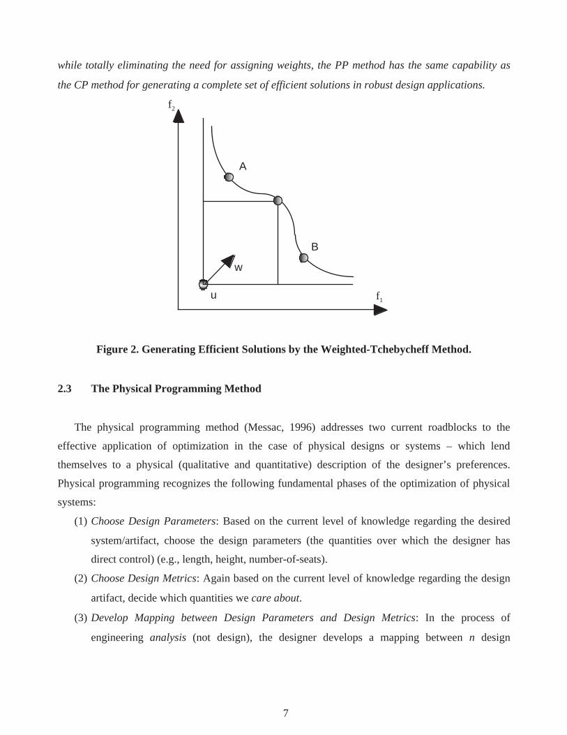
The CP (∞, w) , referred to as the weighted Tchebycheff approach, is found to be very useful in

generating Pareto solutions. The CP formulation is equivalent to the following β-problem

Minimize β

subject to wi( fi(x) − ui) ≤ β , i=1, .., m (2.3)

x ∈ X,

where β is a positive variable, and ui is the ideal solution of the ith design metric. Collectively, the

ui’s define the so-called utopia point. Bowman (1976) shows that for every Pareto solution there

exists a positive vector of weights so that the corresponding CP(∞, w) is solved by this Pareto point.

This result determines the fundamental difference between the WS approach and the weighted

Tchebycheff approach. While the former cannot generate every Pareto solution, the latter can. Figure

2 shows the same efficient frontier that is depicted in Figure 1. For the given utopia point, u, and the

weight vector, w, the solutions of CP (∞, w) can be geometrically identified as the points of contact

between the efficient frontier and the corresponding level curve of the weighted Tchebycheff metric.

We observe that (see Fig. 2), as we change the weights, we may reach all the efficient points located

on the arc between points A and B. In Chen et al. 1999, the CP method is used as a part of an

interactive robust design procedure. The latter guarantees that different combinations of weights

generate a complete set of efficient robust design solutions. In this paper, we aim to illustrate that

7

while totally eliminating the need for assigning weights, the PP method has the same capability as

the CP method for generating a complete set of efficient solutions in robust design applications.

A

B

w

u f1

f2

Figure 2. Generating Efficient Solutions by the Weighted-Tchebycheff Method.

2.3 The Physical Programming Method

The physical programming method (Messac, 1996) addresses two current roadblocks to the

effective application of optimization in the case of physical designs or systems – which lend

themselves to a physical (qualitative and quantitative) description of the designer’s preferences.

Physical programming recognizes the following fundamental phases of the optimization of physical

systems:

(1) Choose Design Parameters: Based on the current level of knowledge regarding the desired

system/artifact, choose the design parameters (the quantities over which the designer has

direct control) (e.g., length, height, number-of-seats).

(2) Choose Design Metrics: Again based on the current level of knowledge regarding the design

artifact, decide which quantities we care about.

(3) Develop Mapping between Design Parameters and Design Metrics: In the process of

engineering analysis (not design), the designer develops a mapping between n design

8

parameters and the m design metrics. This mapping may involve a simple designer-written

code or possibly a large structural analysis software.

(4) Develop Aggregate Objective Function: To reflect the design preference with regard to the

each of the design metrics, these are combined to form an Aggregate Objective Function. The

weighted-sum method is one of the most popular, easiest, – and unfortunately - least effective

methods used in forming this aggregation (Messac, 2000a).

(5) Perform Computational Optimization: Using any number of possible optimization codes,

optimize the aggregate objective function formed in Step-4, subject to provided constraints.

We note that Steps (1), (2), (3), and (5) involve relatively well defined tasks for which generally

mature procedures exist. Parenthetically, we also note that it may be helpful to reverse Steps (1) and

(2) in practice, although in the algorithmic optimization implementation, Step (1) precedes Step (2).

This 5-Step process is only as effective as its weakest links – which in this case is by far Step-4.

There is today no widely-accepted and reliable method for forming the Aggregate Objective Function

in the design process. Performing this task usually involves a largely undefined trial-and-error

weight-tweaking process that may be a source of frustration and significant inefficiency. It is not

uncommon to wait long hours for an optimization run to end, only to realize that the aggregate

objective function was significantly incorrect (one of the weights might have been too small, and the

resulting design undesirable). Therefore, making Step-4 an effective phase of the design optimization

process is one of the two critical aims of the physical programming method.

The other aim of physical programming (PP) is to provide ease of use, as well as robust

computational effectiveness, for novices and experts alike. The notion of dealing with numerical

weights to attempt to describe designer preference is regarded as distinctly unfriendly and ineffective.

When we have to determine, say, six weights, and we discover at the conclusion of an unsuccessful

optimization run that two of these weights are too small (e.g., 100, 0.01) and one is too high (e.g.,

50), we are faced with a truly difficult question. Should we reset these weights at (150, 0.15) and

(30), respectively, or to some other set of numbers? As we can see, this ad hoc weight-tweaking

process can be precarious even for the expert in the art and science of computational optimization.

Physical programming (PP) removes the weight-tweaking process entirely, and allows the designer to

define his/her preference in physically meaningful terms. Physical programming does not require the

designer to specify optimization weights in the problem formulation phase. Rather, the designer

9

specifies ranges of different degrees of desirability for each design metric. PP also addresses the

inherent multiobjective nature of design problems, where multiple conflicting objectives govern the

search of the best solution. Following is a brief description of the procedure for applying physical

programming.

Design Metrics

The problem formulation involves identifying those characteristics of the system or design that

allow the designer to judge the effectiveness of the outcome. Those characteristics, design metrics,

are denoted by gi, and are components of the vector g = {g1, g2 ....}. The elements gi represent

behavior. Design metrics may be quantities that the designer wishes to minimize; maximize; take on

a certain value (goal); fall in a particular range; or be less than, greater than, or equal to particular

values. The designer defines his/her preferences regarding each design metric by specifying

numerical values associated with each. This process is explained later.

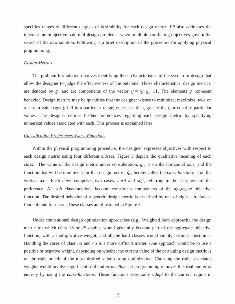
Classification Preferences, Class-Functions

Within the physical programming procedure, the designer expresses objectives with respect to

each design metric using four different classes. Figure 3 depicts the qualitative meaning of each

class. The value of the design metric under consideration, gi , is on the horizontal axis, and the

function that will be minimized for that design metric, gi , hereby called the class-function, is on the

vertical axis. Each class comprises two cases, hard and soft, referring to the sharpness of the

preference. All soft class-functions become constituent components of the aggregate objective

function. The desired behavior of a generic design metric is described by one of eight sub-classes,

four soft and four hard. These classes are illustrated in Figure 3.

Under conventional design optimization approaches (e.g., Weighted Sum approach), the design

metric for which class 1S or 2S applies would generally become part of the aggregate objective

function, with a multiplicative weight; and all the hard classes would simply become constraints.

Handling the cases of class 3S and 4S is a more difficult matter. One approach would be to use a

positive or negative weight, depending on whether the current value of the pertaining design metric is

on the right or left of the most desired value during optimization. Choosing the right associated

weights would involve significant trial-and-error. Physical programming removes this trial and error

entirely by using the class-functions. These functions essentially adapt to the current region in

10

objective space during optimization. Relative emphasis to minimizing or maximizing a given design

metric is dictated by the shape of the class-function. The latter’s shape depends on the stated

preference of the designer.

.

SMALLERIS

BETTER(Class–1)

LARGERIS

BETTER(Class–2)

VALUEIS

BETTER(Class–3)

SOFT HARD

1–S

3–H

2–H

3–S

2–S

1–H

g g

g

gg

g

g

g

g

g

g

g

FEASIBLE

FEASIBLE

FEASIBLE

FEASIBLE

FEASIBLE

INFE

ASIB

LE

INFE

ASIB

LE

INFE

ASIB

LE

INFE

ASIB

LE

INFE

ASIB

LE

INFE

ASIB

LE

INFE

ASIB

LE

INFE

ASIB

LE

RANGEIS

BETTER(Class–4)

4–S

g

INFE

ASIB

LE

INFE

ASIB

LE 4–H

g

g FEASIBLE

INFE

ASIB

LE

INFE

ASIB

LEg

Figure 3. Classification of preference for each design metric

The class functions, shown in Fig. 3, provide the means for a designer to express a range of

preferences for each given design metric. As shown in Figure 3, the soft class functions provide

information that is deliberately imprecise. By design, the utopian value of the class functions is zero.

Next, we explain how quantitative specifications are associated with each design metric.

Physical Programming Lexicon

As mentioned previously, physical programming allows the designer to express preferences with

regard to each design metric. The PP lexicon comprises terms that characterize the degree of

desirability of six ranges for each generic design metric for classes 1S and 2S, ten ranges for classes

11

3S, and eleven for class 4S. Consider for example the case of class 1S, shown in Fig. 4. The ranges

are defined as follows, in order of decreasing preference:

Highly Desirable range (gi ≤ gi1 ): An acceptable range over which the improvement that results

from further reduction of the design metric is desired, but is of minimal additional value.

Desirable range (gi1 ≤ gi ≤ gi2 ): An acceptable range that is desirable.

Tolerable range (gi2 ≤ gi ≤ gi3 ): An acceptable, tolerable range.

Undesirable range (gi3 ≤ gi ≤ gi4 ): A range that, while acceptable, is undesirable.

Highly Undesirable range (gi4 ≤ gi ≤ gi5 ): A range that, while still acceptable, is highly

undesirable.

Unacceptable range (gi ≥ gi5 ): The range of values that the generic design metric may not take.

The parameters gi1 through gi5 are physically meaningful values that are provided by the

designer to quantify the preference regarding the ith generic design metric. These values delineate

ranges of differing degrees of desirability.

The class functions map design metrics into non-dimensional, strictly positive real numbers.

This mapping, in effect, transforms design metrics with disparate units and physical meaning onto a

dimensionless scale through a unimodal function. Figure 4 illustrates the mathematical nature of the

class functions and shows how they allow a designer to express ranges of differing desirability, or

preferences, for a given design metric. Consider the first curve of Figure 4: the class function for a

class 1S design metric. Six ranges are defined. The parameters gi1 through g

i5 are specified by the

designer. When the value of the design metric, gi, is less than g

i1 (highly-desirable range), the value of

the class function is small; thereby requiring little further minimization of the class function. When,

on the other hand, the value of the design metric, gi, is between g

i4 and g

i5 (highly-undesirable range),

the value of the class function is large; which requires significant minimization of the class function.

The behavior of the other class functions is indicated in Figure 4. As we can see, the value of the

class function for each design metric governs the optimization path in objective space with regard to

that design metric.

12

Physical Programming Mappings

We now briefly discuss the various mappings that take place in the implementation of physical

programming, which will define the path from design parameters to aggregate objective function.

The latter is the actual function that the nonlinear programming code minimizes. Figure 5 shows

these various mappings.

TOLE

RA

BLE

HIG

HLY

UN

DE

SIR

AB

LE

UN

AC

CE

PTA

BLE

HIG

HLY

DE

SIR

AB

LE

gi

CLASS-1S

UN

DE

SIR

AB

LE

gi2gi1 gi3 gi4 g i5

g i

TOLE

RA

BLE

TOLE

RA

BLE

DE

SIR

AB

LE

HIG

HLY

UN

DE

SIR

AB

LE

UN

AC

CE

PTA

BLE

HIG

HLY

DE

SIR

AB

LE

gi

UN

DE

SIR

AB

LE

gi2 g i1gi3gi4g i5

gi

TOLE

RA

BLE

CLASS-2S

TOLE

RA

BLE

DE

SIR

AB

LE

HIG

HLY

UN

DE

SIR

AB

LE

UN

AC

CE

PTA

BLE

gi

UN

DE

SIR

AB

LE

gi1

TOLE

RA

BLE

UN

AC

CE

PTA

BLE

DE

SIR

AB

LE

TOLE

RA

BLE

UN

DE

SIR

AB

LE

gi

g i5L g i4L g i3L g i2L g i2R g i3R

HIG

HLY

UN

DE

S.

gi4R g i5R

CLASS-3S

TOLE

RA

BLE

HIG

HLY

UN

DE

SIR

AB

LE

UN

AC

CE

PTA

BLE

gi

UN

DE

SIR

AB

LE

UN

AC

CE

PTA

BLE

DE

SIR

AB

LE

TOLE

RA

BLE

UN

DE

SIR

AB

LE

gi

g i5L

HIG

HLY

-UN

DE

S.

CLASS-4S

HIGHLY-DESIRABLE gi1Rg i4L gi3L g i2L

gi2R g i3Rg i4Rgi5Rg i1L

DE

SIR

AB

LE

TOLE

RA

BLE

DE

SIR

AB

LE

Figure 4. Class-function ranges for the i-th generic design metric.

13

Figure 5. Physical Programming Mappings

As illustrated in Figure 5, we begin with the design parameters, x, over which the designer has

direct control. The design parameters are mapped into the design metrics. Numerically (as

represented by the preference function) the goodness of a given design metric, gi, depends (1) on the

value of the design metric, (2) on the class-type assigned to the design metric (e.g. smaller-is-better),

and (3) on the range of values associated with the design metric (gi1

to gi5

). Loosely speaking, the

sum of all the class functions, which represent mappings of the design metrics, equals the aggregate

objective function (see Messac, 1996, for details).

14

Physical Programming Problem Model

With the mappings described above, the physical programming problem model takes the form

minx g x = log101

nscgi gi xΣ

i =1

n(for soft classes) (2.4)

Subject to

gi(x) ≤ gi 5 (for class 1S design metrics)

gi(x) ≥ gi 5 (for class 2S design metrics)

gi 5L ≤ gi(x) ≤ gi 5R (for class 3S design metrics)

gi 5L ≤ gi(x) ≤ gi 5R (for class 4S design metrics)

gi(x) ≤ giM (for class 1H design metrics)

gi(x) ≥ gim (for class 2H design metrics)

gi(x) = giv (for class 3H design metrics)

gim ≤ gi (x) ≤ giM (for class 4H design metrics)

xjm ≤ x j ≤ x jM (for design var. constraints),

where gim , giM , xjm , and xjM represent minimum and maximum values, and the giv ’s help define

the equality constraints; the range limits are provided by the designer (see Fig. 4); nsc is the number

of soft design metrics that the problem comprises. Note that the aggregate objective function only

comprises class functions associated with soft design metrics. The hard design metrics are, by

definition, treated as constraints. We believe that this lexicographic nature of the design optimization

formulation should be avoided whenever practical. Using the soft classes is often a beneficial

alternative. The log in Eq. 2.4 is present primarily for numerical conditioning purposes.

The above problem model conforms to the framework of most nonlinear programming codes,

with possible minor rearrangements. For further PP-based robust design, see Messac and Sundararaj

2000b. We now apply the above development to two bi-objective robust design problems.

15

3 EXAMPLE PROBLEMS

In this section, two example problems, one a mathematical problem and one a propulsion

system robust design problem, are used to illustrate the effectiveness of the proposed approach.

3.1 A Mathematical Problem

The mathematical problem example is stated as

3 4 21 1 2min ( ) ( 4.0) ( -3.0) ( 5.0) 10.0

xf x x x x= − + + − + (3.1)

Subject to

1 2( ) 6.45 0g x x x= − − + ≤

1 ≤ x1 ≤ 10

1 ≤ x2 ≤ 10

The optimal solution of the above problem is located at the point x = (1.21280, 5.23742), with f(x)

= -1.39378. The bi-objective robust design formulation for the mathematical problem is as follows:

Minimize * *,f f

f f

μ σμ σ

⎡ ⎤⎢ ⎥⎢ ⎥⎣ ⎦

(3.2)

Subject to

1 1 2 1 1 2 2( ) 6.45g x x x k x k x= − − + + Δ + Δ� ≤0

1 + Δx1 ≤ x1 ≤ 10 − Δx1,

1 + Δx2 ≤ x2 ≤10 − Δx2,

where the mean and the variation functions can be approximately derived by using a first-order

Taylor expansion and letting the design parameters’ tolerance be defined as / 3xΔ . This yields

3 4 2

1 1 2( ) ( 4.0) ( 3.0) ( 5.0) 10.0f x x x xμ = − + − + − + (3.3)

and

2 3 2 21 1 2( ) (3.0( 4.0) 4.0( 3.0) ) (2.0( 5.0))

3fxx x x xσ Δ= − + − + − (3.4)

16

When the size of variation is assumed to be 1 2 1x xΔ = Δ = , the ideal solution is obtained as (μ f* ,σ f

* )=

(5.10464, 0.416796), where μ* = μ(xμ f

* ), xμ f

* =(2.00000, 6.45074), σ* = μ f (xσ f

* ) and xσ f

* =(3.50559,

4.99187). After normalization, the ideal solution becomes (μ f* / μ f

* ,σ f* / σ f

* ) = (1, 1). To solve the

above problem using the CP approach based on the formulation in Eq. (2.3), the utopia point is given

as u* =(0.0,0.0).

In Chen et al., 1999, a comparison is made between the solutions obtained from the WS method

and the CP method for the above problem. It was illustrated that, for eighteen evenly distributed

combinations of 1w and 2w , the results obtained from the WS and CP are of radically different

natures. This example clearly illustrates that the CP method can generate a complete efficient set that

has a non-convex portion (which the WS method is unable to generate). We now apply PP to the

same problem.

As mentioned in the description of the PP method (Section 2.3), the foremost task in applying

the PP method is the identification of performance quantities of interest to the designer. Once the

quantities of interest have been identified, they are classified into hard or soft classes. The

mathematical problem under investigation has two objectives. These are: minimization of the mean

(μf ) , and minimization of the variation (σ f ). These two objectives yield two Class-1S design metrics

(Smaller-Is-Better (SIB)). The only constraint, g(x), in Eq. 3.1 is treated, by definition, as a hard

design metric.

Once we determined the preference class of the design metrics, we test a set of preference

structures that capture a variety of design scenarios, which represent different preferences on the

mean and variation of performance. Based on the preliminary study using the CP method, we know

that, after normalization, the best achievable mean is 1 and the worst possible mean (corresponding

to the best achievable variation) is 1.9463. The best achievable variation is 1 and its worst possible

value is 6.8087 (corresponding to the best achievable mean). We formulate a set of preference

structures (see Table 1) with the desirable values falling into the range of the best achievable and the

worst possible values. It should be noted that the use of PP does not require prior knowledge of this

range. In other words, the performance of the PP method is not dependent on whether the desirable

values are chosen inside or outside of this range (Messac et. al. 2000c and 2000d). In this work,

17

different scenarios are constructed to investigate the ability the PP method to generate the complete

efficient frontier. In actual applications, the choice of preference will be problem specific. For further

information on the generation of the Pareto frontier using PP, see Messac et. al. 2000d.

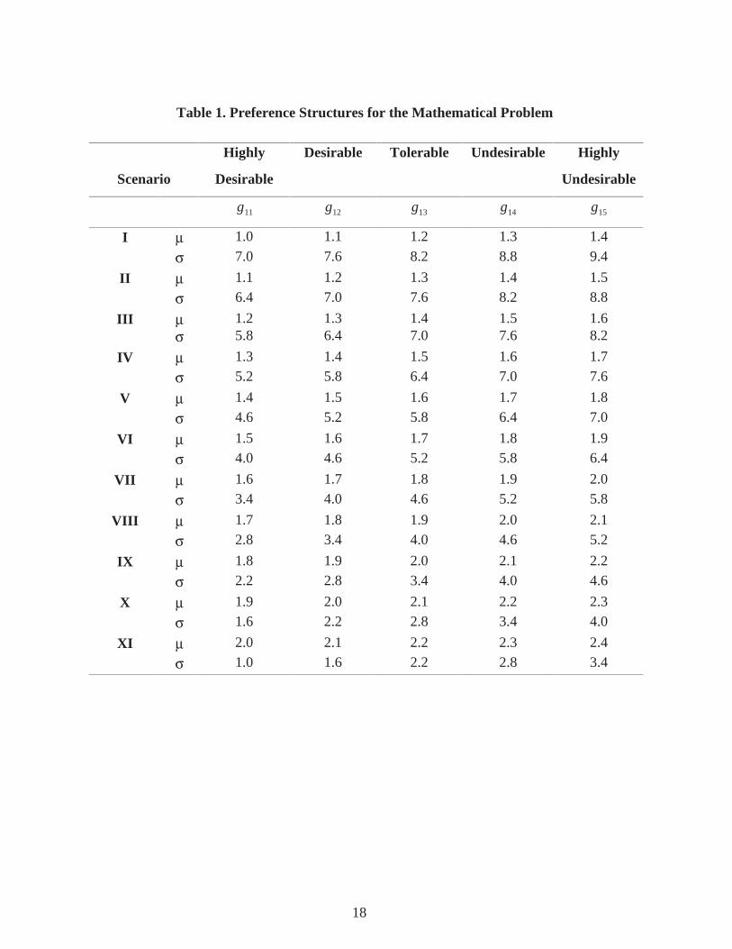
As shown in Table 1, under each scenario for both mean and variation, five values are used to

define the regions highly desirable, desirable, tolerable, undesirable, and highly undesirable. It is

noted that from Scenario I to XI, the designer’s degree of preference for minimizing the mean

decreases, while the degree of preference for minimizing the variation increases. This is reflected in

the shifted regions of the five preference ranges. The simplest approach to choosing the preferences is

to add a constant to each row from scenario to scenario (row to row) in Table 1. In this way, we can

test whether the PP method will be able to generate the Pareto solutions across the entire efficient

frontier. Mean and variation are expressed by specifying their class functions and their associated

ranges.

The robust design problem is solved for each of these scenarios using the PP method and the

solutions are presented in Table 2, and compared with those obtained using the WS and CP methods

for eleven weight settings of (1.0,0.0), (0.9, 0.1), (0.8, 0.2), (0.7, 0.3), (0.6, 0.4), (0.5, 0.5), (0.4, 0.6),

(0.3, 0.7), (0.2, 0.8), (0.9, 0.1), (1.0, 0.0); see Figure 6.

1 1.2 1.4 1.6 1.8 21

2

3

4

5

6

7

Normalized Mean Values

PPCPWS

Nor

mal

ized

Sta

ndar

d D

evia

tion

Valu

es

Figure 6. Comparison of Efficient Solutions for the Mathematical Problem.

18

Table 1. Preference Structures for the Mathematical Problem

Scenario

Highly

Desirable

Desirable Tolerable Undesirable Highly

Undesirable

11g 12g 13g 14g 15g

I μ 1.0 1.1 1.2 1.3 1.4

σ 7.0 7.6 8.2 8.8 9.4

II μ 1.1 1.2 1.3 1.4 1.5

σ 6.4 7.0 7.6 8.2 8.8

III μ 1.2 1.3 1.4 1.5 1.6σ 5.8 6.4 7.0 7.6 8.2

IV μ 1.3 1.4 1.5 1.6 1.7

σ 5.2 5.8 6.4 7.0 7.6

V μ 1.4 1.5 1.6 1.7 1.8

σ 4.6 5.2 5.8 6.4 7.0

VI μ 1.5 1.6 1.7 1.8 1.9

σ 4.0 4.6 5.2 5.8 6.4

VII μ 1.6 1.7 1.8 1.9 2.0

σ 3.4 4.0 4.6 5.2 5.8

VIII μ 1.7 1.8 1.9 2.0 2.1

σ 2.8 3.4 4.0 4.6 5.2

IX μ 1.8 1.9 2.0 2.1 2.2

σ 2.2 2.8 3.4 4.0 4.6

X μ 1.9 2.0 2.1 2.2 2.3

σ 1.6 2.2 2.8 3.4 4.0

XI μ 2.0 2.1 2.2 2.3 2.4

σ 1.0 1.6 2.2 2.8 3.4

19

Table 2. Efficient Solutions of the Mathematical Problem using the PP method

Pareto SolutionsScenario

x1 x2

Normalized

Mean

Normalized

Variation

I 2.00 6.45 1 6.81

II 2.07 6.38 1.07 6.73

III 2.26 6.19 1.26 6.28

IV 2.39 6.06 1.39 5.76

V 2.51 5.94 1.50 5.17

VI 2.63 5.81 1.59 4.51

VII 2.76 5.69 1.68 3.80

VIII 2.90 5.55 1.76 3.01

IX 3.09 5.36 1.84 2.09

X 3.27 5.18 1.89 1.36

XI 3.47 5.00 1.94 1.01

As shown in Table 2, the results obtained using the PP method reflect a tradeoff relationship

between mean, μf , and variation, σf , which is consistent with the preference structures that are

specified. The PP method has been as successful as the CP method in capturing the Pareto set. The

achieved normalized mean varies from 1.0 to 1.9398, and the achieved normalized variation ranges

from 1.0053 to 6.8054. This is very consistent with the range of solutions obtained from the CP

method. From Figure 6, we note that the efficient solutions obtained by the PP method are fairly

evenly spread across the efficient frontier, and that PP captures those points on the Pareto set that lie

in the non-convex region. Since the efficient frontiers obtained from three methods (WS, CP and PP)

overlap with each other, we conclude that the solutions obtained from the PP method belong to the

same efficient frontier as that of the CP method. Hence, the PP and CP methods seem to be equally

effective. Comparing the PP method and the CP method, we observe that it is easier to reach the two

end-points of the efficient frontier when applying the CP method with the weight settings close to

(1.0, 0) or (0, 1.0). We don’t believe this situation to be a hindrance since it is a trivial matter to

obtain these points by minimizing each design metric independently.

20

3.2 Propulsion systems design problem

A propulsion system design problem is used to further illustrate the effectiveness of this paper’s

approach. The design of an aircraft propulsion system is an example of the complex system design

processes that are required for today’s high technology systems. Since the characteristics of the

propulsion system determine approximately 1/3 of the aircraft system direct operating cost and 1/5 of

the total operating cost, it is desirable to select the combination of design parameters that produce the

lowest reasonable cost. There are several fundamental design parameters that relate to the overall

system configuration and to various components, which make up the system. External requirements

and criteria exist from both the airframe manufacturer and the airline that will operate the aircraft. For

example, functional items such as thrust, acoustics and emissions address the suitability of a given

propulsion system to power a particular aircraft; performance items such as fuel efficiency, reliability,

and cost are critical to the operating cost for the airline. In addition, internal company requirements

must be met. These can include technology and manufacturing capability, manufacturing cost and

other profitability parameters, and the potential for adapting existing products to new applications.

The conceptual design of a 30,000 lb. Thrust propulsion system, currently being developed at the

Advanced Engine Programs at Pratt and Whitney for a twin-engine commercial transport is selected

for this study. The results obtained in this paper are based on this propulsion system using the cycle-

module SOAPP (State of the Art Performance Program), with additional weight and drag

correlation’s, as the engine simulation program.

A total of five engine cycle parameters are considered as the design parameters, which are

modeled as the to-be-determined top-level engine design specifications. The upper and the lower

bounds of these parameters are specified in Table 3a. The three constraints, i.e., Overall Pressure

Ratio (OPR), the Fan Diameter (FANDIA), and the High Pressure Turbine Pressure ratio (HPTPR);

and four design metrics, i.e., stream-tube TSFC (SFCWIL), isolated pod TSFC (SFCISO), fuel

burned (FBURN), and range (RANGE) are specified in Table 3b.

Six noise parameters are also introduced for the Robust Design definition. The majority of the

noise factors considered in this study belong to the category of efficiency of the propulsion system

components, such as the fan and compressors. The nominal values for each of them, along with the

21

associated variations, are shown in Table 4. The variations pertain to the final component

characteristics after product design and development.

Table 3. Engine Design Problem IdentificationTop-Level Design Specifications of the Propulsion System Design

Design Parameters Lower Bound Upper Bound Baseline

Fan Pressure Ratio (FPR) 1.25 1.6 1.32Exhaust Jet Velocity Ratio (VJR) 0.6 0.9 0.85Turbine Inlet Temperature (CET) [R] 2400 3000 2750High Compressor Pr. Ratio (HPCPR) 10.2 25 10.2Low Compressor + Fan Root Pressure Ratio (LPCPR) 1.15 4.9 2.14Engine Type TurboFan, Geared TurboFan and ADP GTF

Engine Design – Constraints and ObjectivesConstraints Limits Baseline

Overall Pressure Ratio (OPR) •50 21.8Fan Diameter (FANDIA) • 90 in. 84.3

HP Turbine Pressure Ratio (HPTPR) • 6.0 3.156Objectives Targets Baseline

MIN Streamtube TSFC (SFCWIL) 0.45 lb/hr/lb 0.533MIN Isolated Pod TSFC (SFCISO) 0.45 lb/hr/lb 0.585

MIN Fuel Burn (FBURN) 7500 lbs 8248.1MAX Aircraft Range (RANGE) 3000 nmi 2300.5

Table 4. Noise Parameters for the Engine Design

Noise Parameters Minimum Nominal MaximumFan Efficiency, efnod 0.917 0.927 0.937

Low Compressor Efficiency, elpc 0.89 0.90 0.91High Compressor Efficiency, ehpc 0.881 0.891 0.901

Low Turbine Efficiency, elpt 0.923 0.933 0.943High Turbine Efficiency, ehpt 0.89 0.90 0.91

Fan Duct Loss, product 0.007 0.0075 0.008

In the robust design considered in this study, the ranges of values for engine design parameters,

which are used to optimize the engine performance and minimize the performance deviations, are

identified. The mathematical description of the robust propulsion systems design problem is

presented as follows:

22

Given:

• Models of OPR, FANDIA, HPTPR, RANGE, SFCWIL, SFCISO, and FBURN

• Engine type (TurboFan, Geared TurboFan, ADP), Engine Cycle module configuration

• Noise Factors efnod, elpt, ehpt, elpc, ehpc, and prduct at their mid levels

Find: Robust Engine Design Specifications and the corresponding variations:

• Exhaust Jet Velocity Ratio, VJR, ΔVJR

• Fan Pressure Ratio, FPR, ΔFPR

• Turbine Inlet Temperature, CET, ΔCET

• High Compressor Pressure Ratio, HPCPR, ΔHPCPR

• Low Compressor Pressure Ratio, LPCPR, ΔLPCPR

Satisfy:

• The system constraints

Overall Pressure Ratio, MU_ OPR+ (3*OPR_DEV) ≤ 50

Fan Diameter, MU_ FANDIA + (3*FANDIA_DEV) ≤ 90 inches

High Turbine Pressure Ratio, MU_ HPTPR + (3*HPTPR_DEV) ≤ 6

• The bounds on the system variables:

1.25 ≤ FPR ≤ 1.6 ΔFPR ≥ 3%FPR

0.6 ≤ VJR ≤ 0.9 ΔVJR ≥ 3%VJR

2400 ≤ CET ≤ 3000 ΔCET ≥ 3%CET

10.2 ≤ HPCPR ≤ 25 ΔHPCPR ≥ 3%HPCPR

1.15 ≤ LPCPR ≤ 4.9 ΔLPCPR ≥ 3%LPCPR

Minimize :

[μf , σf ]

where ;

μf =(MU_SFCWIL/0.482) +(MU_SFCISO/0.525) + (MU_FBURN/7364.12) + (2810.24/MU_RANGE)

σf=(DEV_SFCWIL/2.97E-03)+(DEV_SFCISO/1.75E- 03)+(DEV_FBURN/17.28)+(DEV_RANGE/7.99)

The mean and variation values for individual performance (i.e., streamtube TSFC, isolated

pod TSFC, fuel burnt, and aircraft range) have been normalized using the ideal values (best

achievable values). The performance component of the objective function is the sum of the

normalized performance values. Based on the preliminary study using the CP method, we know that

the best achievable μf is 4.04025 and the worst possible μf (corresponding to the best achievable σf) is

4.16256. The best achievable σf is 4.98412 and its worst possible value is 7.92608 (corresponding to

the best achievable μf). A set of preference structures is presented in Table 5. Again, these preference

structures are constructed to test whether the PP method will be able to generate the solutions across

the whole efficient frontier.

23

Table 5 Preference Structures for PP method

Scenario

Highly

Desirable

Desirable Tolerable Undesirable Highly

Undesirable

11g 12g 13g 14g 15g

I μf4.040 4.055 4.067 4.079 4.091

σ f7.926 8.221 8.516 8.811 9.106

II μf4.055 4.067 4.079 4.091 4.103

σ f7.631 7.926 8.221 8.516 8.811

III μf4.067 4.079 4.091 4.103 4.116

σ f7.336 7.631 7.926 8.221 8.516

IV μf4.079 4.091 4.103 4.116 4.128

σ f7.041 7.336 7.631 7.926 8.221

V μf4.091 4.103 4.116 4.128 4.140

σ f6.746 7.041 7.336 7.631 7.926

VI μf4.103 4.116 4.128 4.140 4.152

σ f6.451 6.746 7.041 7.336 7.631

VII μf4.116 4.128 4.140 4.152 4.164

σ f6.156 6.451 6.746 7.041 7.336

VIII μf4.128 4.140 4.152 4.164 4.177

σ f5.861 6.156 6.451 6.746 7.041

IX μf4.140 4.152 4.164 4.177 4.189

σ f5.566 5.861 6.156 6.451 6.746

X μf4.152 4.164 4.177 4.189 4.201

σ f5.271 5.566 5.861 6.156 6.451

XI μf4.164 4.177 4.189 4.201 4.213

σ f4.164 5.271 5.566 5.861 6.156

24

Table 6 Efficient Solutions using the PP method

Scenario Normalized

Mean (μf)

Normalized

Variation (σf)

I 4.0432 7.5989

II 4.0442 7.1601

III 4.0493 6.6869

IV 4.0541 6.3346

V 4.0627 5.8888

VI 4.0704 5.6192

VII 4.0813 5.3858

VIII 4.0955 5.2846

IX 4.1157 5.1845

X 4.1365 5.0838

XI 4.1556 4.9951

The robust design problem is solved for each of these scenarios using the PP method and the

solutions are presented in Table 6, and are compared with those obtained using the WS and CP

methods in Figure 7. The results from the WS and CP methods are obtained by exercising 10 weight

schemes evenly distributed between (0, 1.0) and (1.0, 0).

The efficient frontier formed in the propulsion system design problem is convex. From Figure 7 it

is evident that the WS method generates an uneven distribution of Pareto points for even distribution

of weights. This further confirms the drawbacks of the WS method discussed in the literature. The

CP and PP methods overcome this drawback, which is reflected in Figure 7. This study of the

propulsion systems design problem shows that the numerical procedure employed for the PP method

in this study is in some ways better than that of the CP method. That is, from examining the locations

of the efficient solutions, it is observed that, for a few weight settings, the CP method does not

converge to the global minimum while the PP method does. The preference functions that were used

for the PP method represent the analogs of the weight settings used in the WS and CP methods. The

PP method has been found to generate the most evenly spread set of efficient solutions, when

compared to the WS and CP methods.

25

4.04 4.06 4.08 4.1 4.12 4.14 4.16 4.18

5

5.5

6

6.5

7

7.5

8

Normalized Mean Values

Nor

mal

ized

Dev

iatio

n V

alue

s

PPCPWS

Figure 7. Comparison of Efficient Solutions for Propulsion Systems Design problem

4. CONCLUDING REMARKS

In this paper, we successfully demonstrate the application of the physical programming method

for the generation of efficient robust design solutions that belong to both the convex and non-convex

portions of the efficient frontier. With the PP method, the designer’s preference structure for making

the tradeoffs between the mean and variation attributes are expressed by specifying ranges for each

robustness-related design objective, which indirectly shapes the associated preference function. The

PP method provides a flexible and more natural problem formulation framework for robust design.

Through the example problems, we showed that, in addition to the flexibility it provides in

problem formulation, the PP method also appears to be superior to the popular WS and CP

multiobjective optimization methods in locating the complete set of efficient solutions in an even way.

The PP- and CP-generated solutions may belong to either a convex or non-convex efficient frontier.

The multiple aspects of robust design can thus be addressed explicitly and designers are allowed to

express their preference structures to capture the whole Pareto set. Compared to other robust design

methods, such as the Taguchi’s S/N ratio used as a single criterion, the PP method offers designers he

ability to explicitly address the tradeoff between achieving performance and robustness in the desired

26

proportion. We believe the results of this paper to be of likely general applicability in multiobjective

optimization problems.

ACKNOWLEDEGMENTS

The support from NSF grants DMI 9896300 for Dr. Wei Chen and Grant DMI 97-02248 for Dr.

Achille Messac is gratefully acknowledged. We are also grateful for Pratt & Whitney’s contract on

propulsion systems design.

REFERENCES

Bowman, V. J., 1976, “On the relationship of the Tchebycheff norm and the efficient frontier of

multiple-criteria objectives,” Lecture Notes in Economics and Mathematical Systems, Vol. 135,

pp.76-85.

Box, G., 1988, “Signal-to-Noise Ratios, Performance Criteria, and Transformations,”

Technometrics, Vol. 30, No 1, pp. 1-18.

Chen, W., Allen, J. K., Mistree, F. and Tsui, K.-L., 1996, “A Procedure for Robust Design:

Minimizing Variations Caused by Noise Factors and Control Factors,” ASME Journal of Mechanical

Design, Vol. 118, pp.478-485.

Chen. W., Wiecek, M., and Zhang, J., “Quality Utility: A Compromise Programming Approach

to Robust Design”, ASME Journal of Mechanical Design, 121(2), 179-187, (June 1999).

Das, I. and Dennis, J.E., 1997, “A Closer Look at Drawbacks of Minimizing Weighted Sums of

Objectives for Pareto set Generation in Multicriteria Optimization Problems,” Structural

Optimization, Vol. 14, pp. 63-69.

Hazelrigg, G. A., 1996, Systems Engineering and Approach to Information-Based Design,

Prentice Hall. Upper Saddle River, NJ, USA

Iyer, H.V. and Krishnamurty, S., 1998, “A Preference-Based Robust Design Metric”, 1998

ASME Design Technical Conference, paper no.DAC5625, Atlanta, GA

Keeney, R.L., and Raifa, H., 1976, Decisions with Multiple Objective: Preferences and Value

Tradeoffs, Wiley and Sons, New York.

Messac, A., 1996, "Physical Programming: Effective Optimization for Computational Design",

AIAA Journal, Vol. 34, No. 1, Jan. 96, pp. 149-158.

27

Messac, A., and Hattis, 1996, P., “Physical Programming Design Optimization for High Speed

Civil Transport (HSCT)”, AIAA Journal of Aircraft, Vol. 33, No. 2, pp. 446-449.

Messac, A., and Wilson, B., 1998, “Physical Programming for Computational Control,” AIAA

Journal, Vol. 36, No. 2, pp. 219-226.

Messac, A., Sundararaj, G. J., Tappeta, R. V., and Renaud, J.E., 1999a, "The ability of

Objective Functions to Generate Non-Convex Pareto Frontiers", 40 AIAA/ASME/ASCE/AHS/ASC

Structural Dynamics and Materials Conference, Apr. 12-15, St. Louis, MO. Paper # 99-1211. AIAA

Journal, Vol. 38, No. 3, March 2000.

Messac, A., and Chen, X., 1999b, “Visualizing the Optimization Process in Real-Time Using

Physical Programming,” Engineering Optimization Journal, In Press.

Messac, A., 2000a, “From the Dubious Construction of Objective Functions to the Application

of Physical Programming,” AIAA Journal, Vol. 38, No. 1, pp. 155-163.

Messac, A., and Sundararaj, G. J., 2000b, “A Robust Design Approach using Physical

Programming”, 38th Aerospace Science Meeting, Reno Nevada, January 10-13.

Messac, A., Melachrinoudis, E., Sukam, C. P., 2000c, “Physical Programming: A Mathematical

Perspective”, 38th Aerospace Science Meeting, Reno Nevada, January 10-13.

Messac, A., and Sundararaj, G. J., 2000d “Physical Programming’s Ability to Generate a Well-

Distributed Set of Pareto Points”, 41st AIAA/ASME/ASCE/AHS/ASC Structures, Structural

Dynamics, and Materials Conference, 3-6, April 2000, Atlanta, Georgia.

Nair, V.N., 1992, “Taguchi's Parameter Design: A Panel Discussion,” Technometrics, Vol. 34,

No. 2, pp. 127-161.

Parkinson, A., Sorensen, C. and Pourhassan, N., 1993, “A General Approach for Robust

Optimal Design, ” Transactions of the ASME, Vol. 115, pp.74-80.

Steuer, R.E., 1989, Multiple Criteria Optimization: Theory, Computation and Application, John

Wiley, New York.

Su, J. and Renaud, J. E., 1997, “Automatic Differentiation in Robust Optimization,” AIAA

Journal, Vol. 35, No. 6, pp. 1072.

Sundaresan, S., Ishii, K. and Houser, D.R., 1993, “A Robust Optimization Procedure with

Variations on Design Variables and Constraints,” Advances in Design Automation, ASME DE-Vol.

69-1, pp. 379-386.

Taguchi, G., 1993, Taguchi on Robust Technology Development: Bringing Quality Engineering

Upstream, ASME Press, New York.

28

von Neumann, J., and Morgenstern., O., 1947, Theory of Games and Economic Behavior, 2nd

ed.. Princeton University Press, Princeton, N.J.

Yu, P.L., 1973, “A Class of Solutions for Group Decision Problems,” Management Science,

Vol. 19, pp. 936-946.

Zeleny, M. 1973, Compromise programming, in: Multiple Criteria Decision Making, eds: J. L.

Cochrane and M. Zeleny, University of South Carolina Press, Columbia, SC, pp. 262-301.