Exploration of Nucleon Structure in Lattice QCD with Chiral Quarks MAS by Sergey Nikolaevich Syritsyn L Submitted to the Department of Physics in partial fulfillment of the requirements for the degree of Doctor of Philosophy at the MASSACHUSETTS INSTITUTE OF TECHNOLOGY SACHUSETTS INSTITUTE OF TECHNOLOGY OCT 3 1 2011 LIBRARIES ARCHIVES September 2010 O Massachusetts Institute of Technology 2010. All rights reserved. A uthor ...... .......... - Department of Physics August 2, 2010 Certified by........ John W. Negele William A. Coolidge Professor of Physics Thesis Supervisor Accepted by.. Krishna Rajagopal Associate Head for Education

Welcome message from author
This document is posted to help you gain knowledge. Please leave a comment to let me know what you think about it! Share it to your friends and learn new things together.
Transcript
Exploration of Nucleon Structure in Lattice QCD
with Chiral QuarksMAS
bySergey Nikolaevich Syritsyn L
Submitted to the Department of Physicsin partial fulfillment of the requirements for the degree of
Doctor of Philosophy
at the
MASSACHUSETTS INSTITUTE OF TECHNOLOGY
SACHUSETTS INSTITUTEOF TECHNOLOGY
OCT 3 1 2011
LIBRARIES
ARCHIVES
September 2010
O Massachusetts Institute of Technology 2010. All rights reserved.
A uthor ...... ..........- Department of Physics
August 2, 2010
Certified by........John W. Negele
William A. Coolidge Professor of PhysicsThesis Supervisor
Accepted by..Krishna Rajagopal
Associate Head for Education
2
Exploration of Nucleon Structure in Lattice QCD with
Chiral Quarks
by
Sergey Nikolaevich Syritsyn
Submitted to the Department of Physicson August 2, 2010, in partial fulfillment of the
requirements for the degree ofDoctor of Philosophy
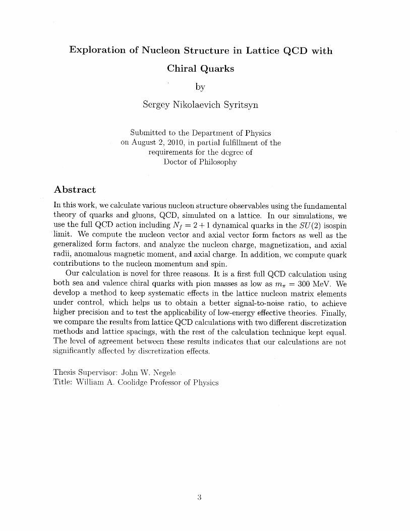
Abstract
In this work, we calculate various nucleon structure observables using the fundamentaltheory of quarks and gluons, QCD, simulated on a lattice. In our simulations, weuse the full QCD action including Nf = 2+ 1 dynamical quarks in the SU(2) isospinlimit. We compute the nucleon vector and axial vector form factors as well as thegeneralized form factors, and analyze the nucleon charge, magnetization, and axialradii, anomalous magnetic moment, and axial charge. In addition, we compute quarkcontributions to the nucleon momentum and spin.
Our calculation is novel for three reasons. It is a first full QCD calculation usingboth sea and valence chiral quarks with pion masses as low as m, = 300 MeV. Wedevelop a method to keep systematic effects in the lattice nucleon matrix elementsunder control, which helps us to obtain a better signal-to-noise ratio, to achievehigher precision and to test the applicability of low-energy effective theories. Finally,we compare the results from lattice QCD calculations with two different discretizationmethods and lattice spacings, with the rest of the calculation technique kept equal.The level of agreement between these results indicates that our calculations are notsignificantly affected by discretization effects.
Thesis Supervisor: John W. Negele .Title: William A. Coolidge Professor of Physics
4
Acknowledgments
This work would not be possible without constant support of many people. I would
like to express my gratitude to my Bachelor's and Master's Thesis supervisor, Mikhail
Polikarpov, who stirred my initial interest in lattice gauge theories by an opportunity
to learn how quantum field theory works in practice and who inspired me with many
exciting examples from quantum physics. A great deal of discussions with Andrew
Pochinsky on the topics of both physics and computer science were often essential
to our progress. During their stay at MIT and after, Harvey Meyer, Massimiliano
Procura, and Meifeng Lin helped tremendously in understanding and interpreting
our calculation results. Michael Engelhardt performed a substantial part of computer
simulations for this project. I am most thankful to my teacher, John Negele, whose
amazing potential to motivate and guide were enormous driving force for this work,
and who has taught me, among other things, how to do Physics with passion.
And, beyond any extent, I am in debt to my family who supported me whole-
heartedly on the difficult path of completing this work.
6
Contents
1 Introduction: Nucleon Structure
1.1 Electromagnetic structure.... . . . . . . . . . . . . . . . . . . . . .
1.2 Axial form factors . . . . . . . . . . . . . . . . . . . . . . . . . . . .
1.3 Generalized form factors.... . . . . . . . . . . . . . . . . . . . . .
2 QCD on a lattice: Overview
2.1 Lattice gauge theory . . . . . . . . . . .
2.1.1 Formulation of QCD on a lattice
2.1.2 Numerical simulation ........
2.2 Discretization of gauge action . . . . . .
2.3 Discretization of fermion action . . . . .
2.3.1 Chiral symmetry on a lattice . . .
2.3.2 Wilson fermions . . . . . . . . .
2.3.3 Domain wall fermions . . . . . .
2.3.4 M ixed action . . . . . . . . . . .
2.4 Rotation symmetry on a lattice .....
3 Nucleon Matrix Elements on a Lattice
3.1 Creating nucleon states on a lattice . . .
3.1.1 Basic nucleon operator . . . . . .
3.1.2 Suppression of excited states
3.1.3 Composite nucleon operators
3.2 Three-point correlators on a lattice . . .
37
. . . . . . 38
. . . . . . 39
. . . . . . 41
. . . . . . 43
. . . . . . 44
. . . . . . 44
. . . . . . 46
. . . . . . 47
. . . . . . 50
. . . . . . 51
3.2.1 Quark-bilinear operators . . . . . . . . .
3.2.2 Connected three-point quark correlators
3.2.3 Composite sources.. . . . . . . . ..
3.3 Form Factors . . . . . . . . . . . . . . . . . . .
3.3.1 Transfer matrix expressions . . . . . . .
3.3.2 Nucleon matrix elements . . . . . . . .
3.3.3 Overdetermined analysis of form factors
3.4 Role of excited states . . . . . . . . . . . . . .
3.4.1 Two-state model...... . . . . . ..
3.4.2 Plateau fits . . . . . . . . . . . . . . . .
4 Renormalization of Lattice Quark-Bilinear Operators
4.1 General aspects of renormalization . . . . . . . . . . . . . . . . . .
4.1.1 Linking lattice calculations and experiment . . . . . . . . .
4.1.2 Mixing of lattice operators . . . . . . . . . . . . . . . . . .
4.1.3 Special cases of lattice renormalization . . . . . . . . . . . .
4.2 Nonperturbative approach to renormalization . . . . . . . . . . . .
4.2.1 Rome-Southampton method . . . . . . . . . . . . . . . . . .
4.2.2 Operators with derivatives . . . . . . . . . . . . . . . . . . .
4.2.3 Quark field renormalization . . . . . . . . . . . . . . . . . .
4.2.4 Vector and axial currents renormalization... . . . . . ..
4.3 Matching to the MS scheme . . . . . . . . . . . . . . . . . . . . . .
4.3.1 Perturbative running of renormalization factors.... . ..
4.3.2 Extraction of scale-independent factors . . . .
4.3.3 Final renormalization coefficients....... ... . . . ..
4.3.4 System atic errors... . . . . . . . . . . . . . . . . . . ..
4.4 Comparison of perturbative and nonperturbative renormalization .
5 Select Results
5.1 I = 1 vector form factors . . . . . . . . . . . . . . . . . . . . . . .
5.1.1 Momentum transfer dependence .
. . . . . . . . . . . . 67
. . . . . . . . . . . . 68
. . . . . . . . . . . . 71
. . . . . . . . . . . . 72
. . . . . . . . . . . . 72
. . . . . . . . . . . . 74
. . . . . . . . . 75
. . . . . . . . . . . . 79
. . . . . . . . . . . . 80
. . . . . . . . . . . . 83
87
87
87
88
90
91
92
93
95
98
99
100
102
104
105
107
111
112
112
5.1.2 Chiral extrapolations using HBChPT+A
5.1.3 Chiral extrapolations using CBChPT
5.2 I 0 vector form factors . . . . . . . . . . . .
5.2.1 Momentum transfer dependence . ..
5.2.2 Chiral extrapolations using HBChPT+A\
5.2.3 Chiral extrapolations using CBChPT .
5.3 Axial form factors . . . . . . . . . . . . . . . .
5.3.1 Axial charge . . . . . . . . . . . . . . .
5.3.2 Momentum transfer dependence . . . .
5.4 Quark energy-momentum tensor . . . . . . . .
5.4.1 CBChPT fits of generalized form factors
5.4.2 Quark momentum fraction . . . . . . . .
5.4.3 Quark angular momentum . . . . . . . .
5.4.4 Quark spin and OAM . . . . . . . . . .
5.5 Generalized form factors . . . . . . . . . . . . .
5.5.1 Momentum transfer dependence . . . . .
. . 118
. . . . . . . . . . . . 126
. . . . . . . . . . . . 129
. . . . . . . . . 129
. . . . . . . . . . . 131
. . . . . . . . . . . . 131
. . . . . . . . . . . . 134
. . . . . . . . . . . . 134
. . . . . . . . . . . . 137
. . . . . . . . . . . . 143
. . . . . . . . . . . . 143
. . . . . . . . . . . . 146
. . . . . . . . . . . . 148
. . . . . . . . . . . . 151
. . . . . . . . . . . . 155
. . . . . . . . . . . . 155
6 Summary
A Lattice QCD simulation ensembles
A. 1 Hybrid action ensembles . . . . . . . . . . . . . . . . . . . . . . . .
A.2 Domain wall fermion ensembles . . . . . . . . . . . . . . . . . . . .
A.3 Wilson-Clover ensembles........ . . . . . . . . . . . . . ...
B Irreducible representations of the hypercubic group H(4)
C Renormalization of lattice operators
C.1 Structure of Born terms and corrections in lattice vertex functions
D Chiral extrapolation formulas
D. 1 Electromagnetic structure................. . . . ...
D.1.1 Small Scale expansion (HBChPT+A ). . . . . . . . . . . .
161
165
165
166
167
169
171
171
173
173
173
D.1.2 Covariant Baryon ChPT (CBChPT ) . . . . . . . . . . . . . . 177
E Abbreviations 183
List of Figures
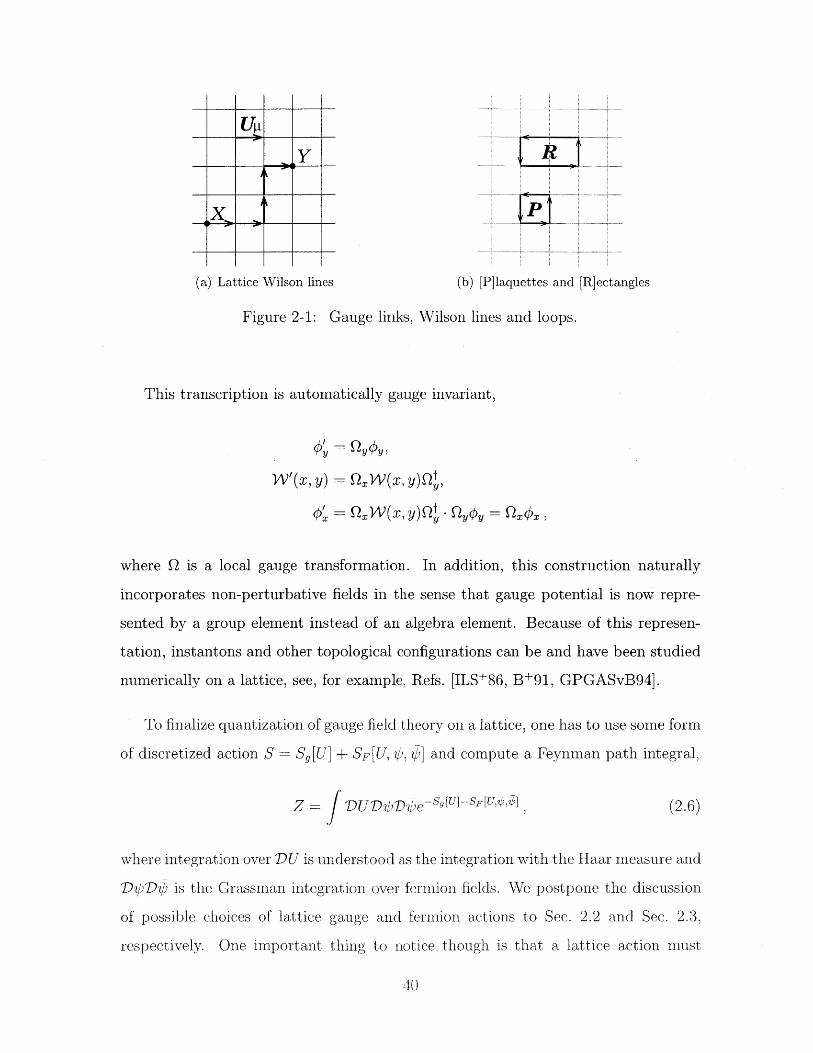
2-1 Gauge links, Wilson lines and loops . . . . . . . . . . . . . . . . . . . 40
3-1 Scan of the Wuppertal and APE smearing parameter space. . . . . . 60
3-2 Source optimization criterion (3.23) vs smeared source r.m.s. radius (3.13).
3-3 Eigenvalues extracted from the nucleon correlator matrix with 8 com-
posite sources and sinks (3.28). . . . . . . . . . . . . . . . . . . . . .
3-4 Wick contractions of quark fields in three-point correlators. . . . . .
3-5 Comparison of the nucleon isovector form factors extracted from the
full overdetermined system, only nonzero equations, uncorrelated fit
the system with averaged equivalent equations (avg-equiv), for the mo-
mentum combinations listed in Tab. 3.2. These types of analysis are
also described in the text......... . . . .............
3-6 Nucleon isovector form factor plateaus for the lightest m, = 297 MeV
ensemble................... . . . . . . . . . . . . . ..
3-7 Illustration of remarkable cancellation between contaminations in all
P' / 0 and P = 0 two-point correlators. ................
3-8 Suppression factor for the excited state contributions Rio(r) (3.56),
as estimated from fitting the two-point function. ...........
3-9 Comparison of the isovector nucleon form factors extracted from plateau
averages and from fitting plateaus to the formula (3.57). Results are
computed on a fine Domain Wall lattice with m, = 297 MeV, with
T = 12 and T = 14 Euclidean time separations. Horizontal axis corre-
sponds to momentum combinations listed in Tab. 3.2. . . . . . . . . 84
3-10 Comparison of Fjd plateau using coherent backward propagators with
T = 12 and independent backward propagators with T = 14. The
momentum transfer Q2 corresponds to (000|011). . . . . . . . . . . . 84
4-1 Analysis of quark momentum components extracted from quark prop-
agators using Eq. (4.21) . . . . . . . . . . . . . . . . . . . . . . . . . 97
4-2 Comparison of vector and axial vector renormalization constants in the
Domain Wall calculations... . . . . . . . . . . . . . . . . . . . . 99
4-3 Comparison of helicity-dependent and helicity-independent renormal-
ization coefficients for Wilson twist-2 operators. . . . . . . . . . . . . 100
4-4 Perturbative 3-loop running of renormalization coefficients in the RI'
schem e. . . . . . . . . . . . . . . . . . . . . . . . . . . . . . . . . . . 101
4-5 Determination of the scale-independent coefficient (4.33) for the Wilson
twist-2, n = 2 operator, T(3) and T(6) representations. . . . . . . . . . 103
4-6 Determination of the scale-independent coefficient (4.33) for the Wilson
twist-2 n = 3 operator, r (4) and r(8 ) representations... . . . ... 103
4-7 Determination of scale-independent renormalization coefficients in the
Hybrid ensemble. See explanations in the text...... . . . . ... 107
5-1 Results for Fd(Q2) at m , = 297 MeV and the dipole fits with three
different Q2 cutoffs (top panels). The ratios of the lattice results for
Fu-d to the dipole fits using Eq. (5.1) (three bottom panels). .U... 115
5-2 Results for G'-"(Q 2) at m, = 297 MeV and the dipole fits with three
different Q2 cutoffs (top panels). The ratios of the lattice results for
G>-jJ to the dipole fits using Eq. (5.1) (three bottom panels). .... 117
5-3 Lattice results for G -d for the fine and coarse Domain Wall ensembles,
compared with a phenomenological fit [Kel04] to experimental data. 118
5-4 Chiral extrapolations for the isovector radii and the anomalous mag-
netic moment using the O(6 ) SSE formula, with (solid curves) or with-
out (dashed curves) the constant term in Eq. (D.5). (rv) 2 and , )2
are fit simultaneously, and K, is fit separately with CA determined from
the sim ultaneous fit. . . . . . .. . . . . . . . . . . . . . . . . . . . . 122
5-5 SSE chiral fits to the isovector radii and the anomalous magnetic mo-
ment constrained to go through the physical points using the input in
Table 5.4 as well as CA = 1.5 and cv = -2.5 GeV- 1 . The mixed-action
results at m, = 355 MeV are shifted slightly to the right for clarity. 124
5-6 Chiral extrapolation for the nucleon mass using the O(p 4) BChPT
formula in Eq. (D.21). The solid line is the fit to only the fine domain
wall data (solid circles). The square is the coarse domain wall result,
and the diamonds are the mixed-action results from Ref. [WL+09]. . 127
5-7 Simultaneous fit to the isovector radii and anomalous magnetic moment
using the CBChPT formula (solid lines). The SSE formula fits without
the constant term for , - (rv)2 (dashed line). . . . . . . . . . . . . . . 128
5-8 The lattice isoscalar Dirac form factor, Fiu+d(Q 2), dipole fits to it and
the phenomenological fit [Ke104] to experimental data. . . . . . . . . 129
5-9 The isoscalar Pauli form factor, F2+d(Q2), const(Q 2) fits and the phe-
nomenological fit [Ke104] to experimental data. . . . . . . . ... 130
5-10 Linear extrapolations for the isoscalar radii and the anomalous mag-
netic moment. Shown also are the phenomenological values for radii
obtained in Ref. [MMD96] and the experimental value [A+08b] for ,,
(sta rs). . . . . . . . . . . . . . . . . . . . . . . . . . . . . . . . . . . 13 2
5-11 Simultaneous(dashed lines) and independent (solid lines) 0(p 4) BChPT
fits to the isoscalar radii and anomalous magnetic moment. . . . . . 133
5-12 Nucleon axial charge to pion decay constant ratio, gA/F, for Domain
Wall , Hybrid and BMW calculations. The upper right panel shows
bare gA/9v ratio. . . . . . . . . . . . . . . . . . . . . . . . . . . . . . 135
5-13 Chiral extrapolations of the nucleon axial charge for the Domain Wall
and Hybrid calculations. In the two-parameter HBChPT fit gi = 2.5
is set. ............. ...... ............ ........ .136
5-14 Q2-dependence of the nucleon isovector axial form factor G-d(Q2). 138
5-15 Nucleon isovector axial radius (rh).. .................. 139
5-16 Nucleon isovector induced pseudoscalar form factor G"-d(Q2). 140
5-17 Pole mass from a fit using Eq. (5.14) and mpole = m,. . . . . . . . . 141
5-18 Check of GT relation. Rp/A(Q 2 ) from Eq. (5.17) should be extrapo-
lated to Q2 -+ 0 to obtain grN9gN . NLO Chiral perturbation theory
predicts that 1 - grN,97rN '~r' 'r --. ''.--.--.-..-..-.--.--142
5-19 Chiral extrapolations of the isovector generalized form factors A'yd,
Bud, Au-d and their slopes PA,B,C using the Domain Wall calculations. 14420 '20
5-20 Chiral extrapolations of the isoscalar generalized form factors A20,
Bu+d, A2+d using the Domain Wall calculations. . . . . . . . . . . . . 145
5-21 Comparison of the isovector quark momentum fraction from the Do-
main Wall and Hybrid calculations.. . . . . . . . . . . . . . . . . 147
5-22 Comparison of the isoscalar quark momentum fraction from the Do-
main Wall and Hybrid calculations. Disconnected contractions are not
included............................ . . . . .. 148
5-23 Comparison of the isovector quark angular momentum J"-d from the
Domain Wall and Hybrid calculations........ . . . . . . . . .. 149
5-24 Comparison of the isoscalar quark angular momentum jti+d from the
Domain Wall and Hybrid calculations. Disconnected contractions are
not included......................... . . . . . .. 150
5-25 Separate u and d quark contributions to the nucleon spin and their
chiral extrapolations. Disconnected contractions are not included. . . 150
5-26 Comparison of the total quark spin contribution to the nucleon spin
from the Domain Wall and Hybrid calculations. Disconnected con-
tractions are not included..... . . . . . . . . . . . . . . . . . .. 152
5-27 Comparison of the quark orbital angular momentum contributions to
the nucleon spin from the Domain Wall and Hybrid calculations. Dis-
connected contractions are not included....... . . . . . . . . .. 153
5-28 Contributions of the u and d quark spin and orbital angular momenta
to the nucleon spin from the Domain Wall calculations. Disconnected
contractions are not included. . . . . . . . . . . . . . . . . . . . . . . 153
5-29 n = 2 spin-independent generalized form factors from the Domain Wall
calculation. Disconnected contractions are not included in the isoscalar
p arts. . . . . . . . . . . . . . . . . . . . . . . . . . . . . . . . . . . . 155
5-30 n = 2 spin-independent generalized form factors from the Hybrid cal-
culation. Disconnected contractions are not included into the isoscalar
p arts. . . . . . . . . . . . . . . . . . . . . . . . . . . . . . . . . . . . 156
5-31 n = 2 spin-dependent generalized form factors from the Domain Wall
calculation. Disconnected contractions are not included into the isoscalar
p arts. . . . . . . . . . . . . . . . . . . . . . . . . . . . . . . . . . . . 158
5-32 Transverse isovector radii as extracted from dipole fits with momentum
cut Q2 < 0.5 GeV 2 to unpolarized Ao and polarized Ano generalized
form factors. . . . . . . . . . . . . . . . . . . . . . . . . . . . . . . . 158
5-33 Dipole fits to the transverse "density" H"( = 0, Q2) from the Domain
Wall calculations. Disconnected contractions are not included into the
isoscalar parts. . . . . . . . . . . . . . . . . . . . . . . . . . . . . . . 159
16
List of Tables
3.1 Parameters for optimal sources as defined in Eq. (3.14) and (3.24).
3.2 A set of momentum combinations satisfying 1pi l < 1 for the high pre-
cision form factors. . . . . . . . . . . . . . . . . . . . . . . . . . . . .
4.1 Results for the renormalization factors Zinal (4.35) in the Domain Wall
calculations. . . . . . . . . . . . . . . . . . . . . . . . . . . . . . . .
4.2 Comparison of different sources of uncertainty contributing to the de-
termination of lattice renormalization factors. Quoted numbers are
fractional errors. . . . . . . . . . . . . . . . . . . . . . . . . . . . . .
4.3 Comparison of perturbative and non-perturbative renormalization fac-
tors for Hybrid ensemble .. . . . . . . . . . . . . . . . . . . . . . . . .
5.1 Comparison of different fits to the isovector Dirac form factors Fi"-d
with different Q2 cutoffs for the fine Domain Wall lattice, m, =
297 M eV.......... .... . . . . . . . . . . . . . . . . . ...
5.2 Comparison of different fits to the isovector Pauli form factors F2-d
with different Q2 cutoffs for the fine Domain Wall lattice, m, =
297 MeV........ ........ ....... . . . . . . . . ...
5.3 Results for the isovector Dirac and Pauli radii and anomalous magnetic
moment from dipole fits with Q2 < 0.5 GeV 2 . . . . . . . . . . . . . .
5.4 Input values for the low-energy constants in the fits: the nucleon axial
charge gA, the pion decay constant F, and the mass difference A -
MA - IN. These values correspond to the chiral limit m, -- 0. . .
104
106
108
114
114
119
120
5.5 Fit parameters from the SSE fits to the isovector Dirac radius (rI)2,
Pauli radius (r) 2 and the anomalous magnetic moment /-. The HBChPT+A
scale is A = 600 MeV.... . . . . . . . . . . . . . . . . . . . . . . 121
5.6 Input values for the covariant baryon chiral fits. . . . . . . . . . . . .
5.7 Low-energy constants from the O(p4 ) BChPT fit to the fine Domain
Wall lattice results of the nucleon mass. In the "Lattice+Exp" fit we
also impose that the curve goes through the physical point. . . . . .
5.8 Fit parameters for the simultaneous fit to (rv) 2, Kv . (rv)2 and rv using
the 0(p') CBChPT formulas. The scale is set to A = MO. . . . . . .
5.9 Results for the isoscalar Dirac and Pauli mean squared radii and the
anomalous magnetic moment from dipole and linear fits. . . . . . . .
5.10 Fit parameters from the simultaneous fit to (r.)2, is (rs)2 and K. using
Eqs. (D.24), (D.25) and (D.26). . . . . . . . . . .. . . . . . . . . . . .
5.11 Fit parameters from independent fits to (rs)2 , K, . (r) 2 and s using
Eqs. (D.24), (D.25) and (D.26). . . . . . . . . . . . . . . . . . . . . .
5.12 Dipole mass for lattice axial form factor G'-d(Q2). . . . . . . . . . .
5.13 Covariant chiral perturbation theory fits to the forward values of n = 2
generalized form factors at p2 = (2 GeV) 2, using the Domain Wall
calculations. . . . . . . . . . . . . . . . . . . . . . . . . . . . . . . . .
126
127
127
130
132
133
139
144
5.14 Covariant chiral perturbation theory fits to the forward values of n = 2
generalized form factors at p2 = (2 GeV) 2 using the Hybrid calculations. 146
5.15 Covariant chiral perturbation theory extrapolations of the quark angu-
lar momentum contributions to the nucleon spin. The renormalization
scale is p2 = (2 GeV) 2 . . .. . . . . . . . . . . . . . . . . . . . . . .
5.16 Covariant chiral perturbation theory extrapolations of the quark spin
contributions to the nucleon spin................. . ...
149
154
5.17 Covariant chiral perturbation theory extrapolations of the quark or-
bital angular momentum contributions to the nucleon spin. The renor-
inalization scale is p = (2 GeV 2)............... . . ... 154
A.1 Summary of Hybrid ensembles. . . . . . . . . . . . . . . . . . . . . . 165
A.2 Hadron masses and decay constants in lattice and physical units in
H ybrid ensem bles. . . . . . . . . . . . . . . . . . . . . . . . . . . . . . 166
A.3 Summary of Domain Wall ensembles. . . . . . . . . . . . . . . . . . 166
A.4 Hadron masses and decay constants in lattice and physical units in
Domain Wall ensembles.. . . . . . . . . . . . . . . . . . . . . . . 167
A.5 Summary of BMW ensembles......... . . . . . . . . . . . . . . 167
20
Chapter 1
Introduction: Nucleon Structure
Since the early days of hadron physics it has been known that the proton and neutron
are not point-like particles, as indicated by the deviation of their magnetic moments
from the Dirac equation values [Ste33]. Generally speaking, the non-elementary mag-
netic moments mean that there are circulating currents inside nucleons. Elastic e - p
and e - n scattering experiments showed that their spatial electric charge distribu-
tion is also not point-like. Extensive studies of the quark density and helicity inside
protons and neutrons at SLAC, Fermilab, CERN and DESY resulted in the under-
standing that quarks contribute only some part to the boosted nucleon momentum
and spin, and also contribute only a negligible part of its mass. The rest must be
carried by gluons, which are thus essential and separately relevant degrees of freedom
inside a nucleon.
A new generation of dedicated experiments are planned or already underway to
further explore the structure of the nucleon, including COMPASS [A+07], HER-
MES [A+99, KNO2), CEBAF at Jefferson Lab, PANDA at FAIR [Gia10], MAMI [Are06],
RHIC Spin [Vog04] and others. These experiments aim at higher levels of precision in
measuring nucleon form factors, as well as mapping out the three-dimensional struc-
ture of the nucleon and resolving the long-standing "spin crisis" puzzle [A+88b], or
the origin of the nucleon spin.
There is definitely a need for a theory which could explain such a rich and compli-
cated system as a nucleon. Such a theory should be able to make predictions about
nucleon structure and constrain phenomenological analyses of experimental data. A
vital example demonstrating the need for theory constraints is generalized parton
distribution functions (GPDs) [Die03], which describe the contents of a boosted nu-
cleon(see also Sec. 1.3). The GPDs Fq can be measured in inelastic scattering exper-
iments through their convolutions with parton scattering kernels T
amplitude Jd T( ) Fq((,)
and thus are not accessible directly. Dependence of GPDs Fq(x, , t) on its kinematic
variables can reveal the full three-dimensional structure of the nucleon. However,
to extract physics information from such measurements, one has to assume some
functional form for the GPDs (see, e.g., Ref. [DFJK05]) inevitably introducing model
dependence into experimental results. Although quite a few phenomenological models
explaining certain aspects of nucleon structure have been proposed, none of them is
able to solve all of the nucleon puzzles consistently. Apparently, one has to use the
fundamental theory of strong interactions, quantum chromodynamics (QCD), to fully
understand how nucleons and other hadrons are formed from the elementary particles,
quarks and gluons.
Quantum chromodynamics has been successful in explaining high-energy processes
where asymptotic freedom permits perturbative treatment of scattering events. How-
ever, the low-energy phenomena such as confinement, spontaneous chiral symmetry
breaking, the light hadron spectrum and hadron structure definitely require non-
perturbative methods. Numerical calculations on a lattice have proven to be the only
viable tool so far to extract quantitative predictions from non-perturbative QCD. Al-
though currently there are certain limitations in this approach, such as finite volume,
finite ultraviolet cutoff and difficulties in making the pion of simulated QCD as light
as the real-world pion, all these obstacles can, at least in principle, be overcome using
more powerful computers. For example, recently the Budapest-Marseille-Wuppertal
lattice QCD collaboration reported the first successful calculation of hadron spectrum
using full QCD with three dynamical flavors [D+08]. It would be fair to say that the
current predictive power of lattice QCD is limited by available computing resources,
and eventually, as they advance, more accurate calculations with smaller systematic
errors will be possible.
Lattice QCD is a solution of quantum field theory in Euclidean space on a discrete
lattice. The transition to Euclidean space is required to make all particles "virtual"
in the sense that their correlators decay exponentially along any direction. Because
there are no massless particles in the spectrum of QCD, this system may be simulated
in a finite box with the size limited from below by the inverse mass of the lightest
particle, the pion. To study hadron structure on a lattice, one computes matrix
elements of local operators between single-hadron states. For example, charge and
magnetization distributions in the nucleon are extracted from the vector current;
quark and gluon contributions to the nucleon momentum and angular momentum
are extracted from the energy-momentum tensor. Computations with local twist-two
operators that are related to the Mellin moments of the parton distribution functions
(PDFs) provide theoretic constraints which complement experimental measurements.
In principle, using lattice QCD methods one can "measure" any local operators that
are inaccessible experimentally and fill in the gaps in our picture of nucleon properties.
Although applying brute-force calculations to lattice QCD may help to improve
its results, in practice only a combination of advanced error-reduction methods and
increased computer time might lead to good quantitative predictions. The main rea-
son for this is that lattice QCD is a Monte-Carlo simulation, and the associated
stochastic variation decreases only as o-~ where N is the number of stochastic
samples. At the same time, the computational cost of each sample increases drasti-
cally with the linear size of the box and with decreasing quark masses. In addition,
the size of Monte-Carlo ensembles necessary to suppress noise may vary depending
on the quantity being computed. For example, in the baryon spectrum calculations
many cancellations occur that aggravate their stochastic variation. This effect is even
worse in the calculations of hadron structure because one has to compute three-point
correlators as opposed to two-point correlators for the hadron spectrum. The devel-
opment of methods to extract the answer with small stochastic uncertainty, and to
set a bound on lattice QCD-specific systematic bias constitutes a major part of this
work.
In this work we study nucleon structure observables using the most advanced and
systematic bias-free lattice QCD framework, calculations which only recently became
feasible. To produce reliable results from lattice QCD, one has to solve a number
of problems. First, as will be discussed in Chapter 2, the simulation of fermions on
a lattice is difficult because simple discretizations of the fermion action break chiral
symmetry. Chiral symmetry is essential if one wants to preserve the original sym-
metries of the theory and connect the results of simulations to low-energy effective
theories such as chiral perturbation theory (ChPT). Also, it reduces dramatically the
lattice-specific systematic effects, or lattice artifacts, such as unphysical mixing be-
tween operators relevant to the hadron structure. A number of approaches have been
devised to avoid chiral symmetry breaking on a lattice. However, all of them increase
the cost of simulations significantly. The second problem is that light quarks and, cor-
respondingly, light pions are expensive to simulate. In addition to purely numerical
handicaps, one needs larger spatial volume to preserve long-range meson dynamics.
Moreover, the Monte-Carlo update is more difficult because lighter fermions produce
more rigid "feedback" on the color gauge field and finer and more accurate calcu-
lations are required. Finally, as mentioned above, the stochastic variation of lattice
QCD calculations grows as the pion mass decreases. All these difficulties limit the
current simulations with chiral quarks' to pion masses m, > 300 MeV and finite
volume < (3.5 fm) 2 .
Because of the high cost of realistic lattice QCD simulations, we focus on reduc-
ing the uncertainty as much as possible and extracting precise results for nucleon
structure by fully utilizing the statistics available from the existing lattice QCD en-
sembles [A+08a, B+09, B+01]. For example, we have been able to compute the
nucleon electromagnetic structure with a remarkable precision for pion masses down
1 Lattice QCD is a rapidly changing field, which progresses at least as fast as computing resources.
The cited limitations applied in 2007 to the generation of the gauge configurations used in this work.
Lattice QCD results for nucleon structure presented here are up-to-date since they require significant
additional calculations.
to 300 MeV [S+10]. Currently, lattice QCD simulations are performed in the isospin
limit mu = md = m < ms, and the electromagnetic interactions of quarks are ne-
glected. We used these results to check existing predictions from Chiral Perturbation
Theory with the conclusion that ChPT (at least, to the approximation order used)
is not applicable in this range of the pion masses. In addition, it is very reassuring
that we are able to reach the precision of existing experiments, albeit with the up
and down quark masses still being too heavy for a direct comparison. Furthermore,
by comparing the results from several different lattice QCD methodologies, we check
whether QCD discretization has any effect on the lattice QCD predictions. Fair agree-
ment between mixed quark action [B+10] and unitary chiral quark action [LHP, S+10]
shows that lattice QCD gives consistent results.
The rest of this chapter is devoted to the discussion of some of the nucleon struc-
ture observables which we compute from lattice QCD and compare to experiments
and other theoretical models. In Chapter 2 we briefly describe and compare the ways
to implement QCD on a lattice, and discuss their respective advantages and potential
problems. Chapter 3 is an overview of the methods to create nucleon states on a lat-
tice and control related systematic effects. Good control over systematic effects allows
one to reduce stochastic errors without inducing systematic bias. Since the operators
computed on a lattice require renormalization, we performed such renormalization
nonperturbatively and describe the methods we used in Chapter 4. Chapter 5 sum-
marizes the most physically interesting results:
" Nucleon vector form factors for the space-like momentum transfer 0 < Q2 <
1 GeV 2 , nucleon charge and magnetization mean squared radii, anomalous mag-
netic moments.
" Nucleon axial form factors, nucleon axial charge and axial r.m.s. radii.
. Quark contributions to the nucleon momentum, as well as quark spin and orbital
angular momentum contributions to the spin of the nucleon.
* Nucleon generalized form factors (GFFs) for u and d quarks corresponding to
n 1, 2 and 3 moments of generalized parton distributions, revealing the
dependence of the latter on their kinematic parameters.
Wherever possible, we apply chiral extrapolation formulas to obtain the values at the
physical pion mass m, ~ 140 MeV which is a factor 2 less than the lightest mass in
our simulations.
1.1 Electromagnetic structure
Electromagnetic form factors characterize fundamental aspects of the structure of
protons and neutrons. In particular, they specify the spatial distribution of charge
and magnetization. For nonrelativistic systems the electric and magnetic Sachs form
factors GE(Q 2 ) and GM(Q 2 ) (see Eqs. (1.2,1.3)) would just be Fourier transforms
of the charge and current densities. A probabilistic interpretation of the Dirac and
Pauli form factors F1(Q2) and F2 (Q2) (See Eq. (1.1)) can be obtained from a two-
dimensional Fourier transformation to impact parameter space in the infinite mo-
mentum frame [BurOO, Bur03]. At high momentum transfer, the elastic form factor
specifies the amplitude for a single quark in the nucleon to absorb a very large mo-
mentum kick and share it with the other constituents in such a way that the nucleon
remains in its ground state instead of being excited. It thus describes the onset of
scaling [BF75, BJY03] and the scale at which quark counting rules become applicable,
which is an unresolved theoretical question in nonperturbative QCD. Given the con-
stantly improving experimental measurements of form factors and their fundamental
significance, it is an important challenge for lattice QCD to calculate them accurately
from first principles.
The nucleon Dirac and Pauli form factors, F1 (Q2) and F2(Q2), respectively, are
defined as follows for each quark flavor (q):
(P', S'gy'ql, S) =U(P', S') 7KFf(Q2) + i 2 " Fj'(Q2) U(P, S), (1.1)
where U(P, S), U(P', S') are the initial and final nucleon spinors; S, S' are the corre-
sponding spin vectors; the momentum transfer is q = P'- P with Q2 -_ 2 > 0; and
MN is the nucleon mass. The Sachs form factors GE (Q 2 ) and GM(Q 2) are defined by
GE(Q 2) F1(Q2) _ 2F2(Q 2), (1.2)(2MN)2
GM(Q 2) F1 (Q2) F2 (Q 2 ). (1.3)
Finally, it is useful to define isoscalar and isovector form factors as the sum and
difference of proton and neutron form factors as follows:
F2(2) = F 2 (Q 2) - F"2 (Q2 ) Fu2(Q2) -- Pf 2 (Q 2) Flud(Q2), (1.4)
F 2 (Q 2) Ff2 (Q 2) + F"2 (Q 2) 1 (F1 2 (Q2 ) + F 2 (Q 2)) F+d(Q2)
where, according to Eq. (1.1), F'" are the form factors of the electromagnetic current
in a proton and a neutron, respectively:
2 1-1Vem,p = - 2 -- dy"d, V'"m, 1 2-ymd. (1.6)3 3 3m n
Although proton and neutron form factors contain both connected diagrams, cal-
culated in this work, and disconnected diagrams, which are currently omitted, the
disconnected diagrams do not contribute to the isovector form factors F>. Hence, we
will devote particular attention in this work to the isovector form factors.
Precise experimental measurements of the set of all four nucleon form factors re-
mains challenging, and the field is marked both by significant recent developments and
open questions. Although the most straightforward measurement is F1 (Q2) for the
proton, the slope at very small values of Q2 remains controversial. Phenomenological
fits to experimental form factors [FW03, AMT07] appear to be inconsistent with anal-
yses based on dispersion theory [H+76, MMD96, BHM07], with phenomenological fits
yielding larger Dirac radii. Hence, a new generation of precision measurements of form
factors at low momentum transfer is currently being undertaken at Mainz [BerO8].
In addition, a recent measurement of the proton charge radius using the Lamb shift
in the pip system [P+10] disagrees with the earlier results, which may be an indica-
tion that not all the theoretical corrections in these experiments have been assessed
and confirmed. Spin polarization experiments [M+98, P+01, G+02, G+01, P+05]
yielded results for F2(Q2) significantly different from traditional measurements based
on Rosenbluth separation, and there is a consensus that two-photon exchange pro-
cesses contribute much more strongly to the backward cross section used in Rosen-
bluth separation than to polarization transfer [AMT07]. However, there are not yet
precise theoretical calculations of two-photon exchange that fully resolve the discrep-
ancy between the two experimental methods, and hence experiments using positron
scattering, for which the relative contribution of the two-photon term changes sign,
are being prepared [A+04a, OLY09]. Neutron form factors are more uncertain than
proton form factors because of the need to know the nuclear wave function to go
from experimental scattering results from deuterium or 3He to a statement about the
neutron form factor. Over the years, nuclear models and theoretical calculations have
been refined, but it is still a challenge to provide a definitive estimate of the uncer-
tainty in the claimed neutron form factors extracted from nuclear targets. Given the
level of precision to which we aspire in lattice calculations, systematic uncertainties in
isovector and isoscalar form factors are not necessarily negligible. In the future when
lattice calculations reliably include precise calculations of disconnected contributions,
it may well be that lattice calculations play a role in guiding the resolution of some
of these experimental questions.
In Section 5.1 we present our results for the momentum dependence of the nucleon
vector form factors F1 (Q2 ) and F2(Q2 ), their r.m.s. radii
2 6 dF1,2r,2)= F1,2 dQ2
and the nucleon anomalous magnetic moment / = F2 (0). We apply chiral pertur-
bation theory to extrapolate the Dirac and Pauli r.m.s. radii to the physical point.
However, such extrapolation is difficult because these quantities diverge in the chiral
limit.
1.2 Axial form factors
Electroweak probes such as (anti)neutrinos interacting with quarks via chiral currents
give access to the nucleon axial structure [BEM02]. The nucleon axial structure is
characterized by the nucleon axial form factors,
(N(P',S)Aa pj S) -(, S/) PGA(Q2)+ (GP)P (Q2) 15aU(P, S),
(1.7)
where AA = qyl ro5 Taq is the non-singlet axial current. GA(Q 2) is called the nucleon
axial form factor and Gp(Q 2) the induced pseudoscalar form factor at the momentum
transfer Q2 - (p' _ p) 2. On a lattice we work in the isospin-symmetric limit with
M,= Mp =MN, and study the proton matrix elements of the isovector current
A3, " yy _ g'y-y 5d which measures the correlation between the spin and isospin
distributions inside a nucleon.
In experimental measurements, the form factor GA(Q 2) in the range Q2 < 1 GeV 2
is usually parameterized phenomenologically with a dipole formula,
GA(Q 2 ) A9A(1 + Q 2/M) 2 '
where the dipole parameter MA is called the axial mass. In the forward limit Q2 = 0
the axial form factor gives the nucleon axial charge gA = 1.1267(3) [A+08b) which is
known precisely from measurements of neutron #-decay lifetime.
There are two methods to measure the nucleon axial form factor GA(Q 2) for
Q2 / 0. One method is based on (anti)neutrino scattering off protons [A+88a],
deuterons [K+90] or nuclei [KLN+69]. In the other method, GA(Q 2 ) is determined
from charged pion electroproduction off protons (e.g., Ref. [B+73]). The resulting
world averages for the axial masses are
MA = 1.026(21) GeV neutrino scattering,
JVIA = 1.069(16) GeV pion electroproduction,
which disagree by - 4%, which is approximately 1.6o- deviation with their errors.
The axial mass is connected to the mean-squared axial radius, defined through the
low-energy behavior of the axial form factor, assuming the dipole form (1.8) holds for
Q2-__ 0
1 2 6 dGA(Q 2 )GA(Q 2 ) =gA( - -rQ 2 + Q)), ( G ~ + Q 2 Q (1.9)6 GA(0) dQ Q=0
From the two experimental values above, one can extract the axial radius,
(r) = 0.666(14) fm neutrino scattering,
(r) = 0.639(10) fm pion electroproduction
The induced pseudoscalar form factor Gp(Q 2) is expected to receive its dominant
contribution from a pion pole, which reflects the pion-mediated coupling of nucleons
to the axial current:
G -(Q 4MNF,g-rN + 0(Q 0 ). (1.10)
where gYrN = 9(rNQ 2 -mi) is the pion-nucleon coupling constant in N -+ rN
processes and F, ~ 93 MeV is the pion decay constant. Because of the chiral Ward
identity the induced pseudoscalar form factor is not independent of the axial form
factor [BKM94]. This fact is reflected in the Goldberger-Treiman relation
gA=
197N1F
MN
which must hold precisely in the chiral limit and approximately for m, / 0 up
to O(m2) corrections from ChPT. Additionally, from ChPT one can find O(Q 0 )
correction to Eq. (1.10) [BKM94, BEM02]:
Gy(Q2 4 MNF , g7 N -2Am 22 2Gp (Q2) -g4I Fng4N 2 2j) +(Q 2 , MD) (1.12)
m2+Q 2 3A
and this formula is believed to describe Gp well for small momentum transfer Q2.
The induced pseudoscalar form factor can be determined experimentally from
ordinary muon capture (OMC) p + p -+ v,, + n in a pp "atom" at the low fixed
momentum transfer Q20Mc = 0.88m'. However, because of systematic difficulties the
uncertainty is quite large, constituting ~ 30% [BEM02]. In radiative muon capture
(RMC) experiments, where an additional photon is emitted, it is possible to study
timelike momentum transfer values up to Q2 = -m2, which are very close to the
pion pole. However, such events are strongly suppressed by the branching ratio.
Analyses based on the hypothesis of pion pole dominance give values for Gp(Q 2
Q2MC) [J+96, W+98, BF89] that are about 50% larger than expected from theory
and determined from OMC.
Another way to determine the form factor Gp(Q 2 ) is pion electroproduction. The
results [C+93] for the Q2-dependence of Gp agree with pion-pole dominance, but the
precision is not sufficient to separate the pion pole contribution from chiral perturba-
tion theory corrections in the spirit of Eq. (1.12). Currently, the induced pseudoscalar
form factor remains the least known of all electroweak nucleon form factors [BEM02],
which makes its theoretical investigation very important.
We investigate the nucleon axial and induced pseudoscalar form factor on a lattice
and present our results in Sec. 5.3. We compute the nucleon axial charge gA and
axial radius (rA). We also compute the momentum dependence of GA and Gp form
factors and compare them to the phenomenological expectations and experimental
results discussed above. In addition, we attempt to check the pion-pole dominance
hypothesis and the Goldberger-Treiman relations [GT58a, GT58b].
1.3 Generalized form factors
Generalized parton distributions (GPDs) unify and extend the notions of nucleon
parton distributions and nucleon elastic form factors, the principal quantities that
provide information on nucleon structure [DieO3]. Compared to the ordinary parton
distribution functions (PDFs), which simply count the partons with a given longitudi-
nal momentum and polarization, GPDs parameterize scattering amplitudes in which
a parton acquires some momentum from external particle(s), both in longitudinal and
transverse directions. At the same time, compared to the elastic form factors, the
GPDs reveal how the nucleon charge and magnetization are distributed over partons
with different longitudinal momentum fraction. As mentioned before, GPDs depend
on the three kinematic parameters, x, (, and t, and experimental study of GPDs
can potentially provide a three-dimensional image of hadron structure [Buroo]. Also,
knowledge of parton distribution in the transverse plane gives access to the orbital
angular momentum (OAM) of partons.
An attractive feature of the generalized parton distributions is that they occur in
a range of different processes, e.g. deeply virtual Compton scattering [A+01, S+01,
C+03, A+05), wide-angle Compton scattering and exclusive meson production, in
addition to the classic processes that probe the forward parton distributions and
form factors. The challenge of GPDs lies in their more complex structure each
generalized parton distribution is a function of three parameters rather than just
one, and different experimental processes provide different constraints on their form.
Typically only convolutions of these functions in the x variable are experimentally
accessible.
In this work we concentrate on the valence quark GPDs of a nucleon. The GPDs
are defined through matrix elements of bi-local light cone quark operators,
Oq(x) f e i2 q(-An) #W)/(-An, An) q(An), (1.13)
0OY (x) = A eC 2ix(-An) #_Y W (--An, An) q (An), (1.14)
where n is a light-cone vector, n2 = 0, and I is the light-cone Wilson line connecting
points ±An:
V(-An, An) = Pexp - ig J da n -A(an)1
The matrix elements of the operators (1.13,1.14) between single-nucleon states are
parameterized according to their Lorentz tensor structure [Die03]:
(P', S'|OqP, S) =U(P', SI) [#rH(x, (,t) +E±(x, (, t)] U(P, S), (1.15)2MN
(P', S'IOg5 lP, S) U(P', S') [7{5Ht(x, , t) + n q 7y55q(x, , t)] U(P, S), (1.16)2MN
where the frame-independent Lorentz scalars H , Eq are the unpolarized and He,
Eq are the corresponding polarized generalized parton distributions. In this work we
do not analyze the so-called transversity distributions Hj,Ej, which are discussed in
a different publication [Bra09]. The parameters in Eqs. (1.15,1.16) are the average
longitudinal momentum fraction of the struck parton x, the longitudinal momentum
transfer fraction ( = -n -q/2 = (P - P') -n/(P'+ P) -n and the total momentum
transfer squared t = Q2 q2, where q = P' - P.
Since lattice calculations deal with operators and matrix elements in Euclidean
space, a direct computation of non-local light-cone operators is not possible. Instead,
to facilitate the lattice calculations one takes x"- 1-moments of Eqs. (1.15) and (1.16),
yielding a tower of local operators whose matrix elements can be related to the corre-
sponding moments of H, E, H and E. In this study, we will compute matrix elements
of the following local generalized currents,
(O Ly5j ) {k =l.. q Yl4L[n5]i}' 2 - - i q
Curly braces around indices represent the symmetrization of the Lorentz i
p[, . . p, and the subtraction of traces over pairs of these indices. The sym
derivative is defined as D D D)
Taking the x"4 -moments of the GPDs we define the generalized moments
(1.17)
ndices
metric
(1.18)H t) J dx x -1H(x, (, t)
E"n( , t ) dx x"-1 E(x, gt) ,
5"((, t) J dx x"- 5(x , t),
Z"' t) dx x" ZE(x, gt) .
The non-forward nucleon matrix elements of the local operators, Eq. (1.17), can in
turn be parametrized according to their Lorentz structure in terms of generalized
form factors (GFFs) Anmi(t), Anm(t), Bnm(t), Bamn(t), and Cnm(t), for n = 1, 2, 3
S') [7.j1A 1o(t) + i"'q, Bio(t)1 U(P, S),
P', S'l 3912} |P, S) = U(P', S') IP{1p17A /2A 2 o(t) + PIPI 2m B 20 (t)
+ q1qtC20(t) U(P,S),
U(P', S') Lp pb2 1 3A 30 (t) + p{i pbP2 2m B 3 0(t)
+ q{IItq/P2 .ybL3A 3 2 (t) + qlq 112 " 0 B 32 (t)] U(P, 5),2m
(1.19)
for the vector operators and
(P',I) S'I (o5 )1|IP, S) =
(P', IS (0 5)/1AP21 1p, S) =
(P', S'1 (0745){ 192n P ,/3 Ip S) =
U(P', 5') 7175A10(t) + 7'5bo(t)1 U(P, S) ,
U(P', S') Pj17/72I5A20 (t) + q 7IP1 5520(t U(P, S),I ~~2m---WI
U(P', S') Pf/i PA27 P31 7 5A 3o(t) + q{P'1 pP'2 PP3} 755f3 o(t)2m
+ q/l1q uA2Y3IT35 A3 2 (t) + q7Pq525qP3 32(t) , U(P, S)2m
(1.20)
for the axial vector operators. Here we have defined the average nucleon 4-momentum
P = (P'+P)/2. By comparing these expressions with the xn4moments of Eqs. (1.15,1.16)
and using Eq. (1.18), one finds that the i-dependence of the moments of the GPDs
is merely polynomial[Die03],
E"=1 (, t) = Bio(t) ,H"n=1 ((, t) = Aio (t) ,
H =2(, t) = A20 (t) + (2 )2 C2 0(t)
Hn=3(, t) - A30(t) + (2 )2A 32 (t)
E n=2 (, t) B20(t) - (2 )2C20 (t) ,(1.21)
E n=3 (, t) = B 30 (t) + (2 )2B 32 (t) ,
(P', IA S'0 IP, S) U(P',
(P', S'1 IOM 1is~n 1P, S)
,t) = 1 0(t) ,
ftn=2 ( t) A 20 (t) ,
ftn=3 (, t) A30(t) + (2 ) 2 A3 2 (t)
E==l ( , t) b 1 0 (t),
n=2(,t) = b 2 0 (t)
5n=3(,, t) _5 30 (t) + (2 )2532 (t)
In the forward limit of Eqs. (1.15,1.15) with P = P', we obtain the well-known parton
distribution functions,
q(x) = Hq(x, = 0, t = 0) , (1.23)
It is interesting that in the case ( = 0 and arbitrary t = q2, that is when the momen-
tum transfer is limited to the transverse direction, the GPDs and the corresponding
GFFs can be interpreted as distributions in both longitudinal momentum and trans-
verse position in the infinite longitudinal momentum frame [Bur00].
Taking together Eqs. (1.18,1.21,1.22) and Eq. 1.23 and setting t = 0 will similarly
yield the PDF moments
(X"~ 1 )Aq = H5(0, 0) = Ano(0) . (1.24)
Note also that for n = 1 from Eqs. (1.19,1.20) we recover the nucleon vector and
axial form factors introduced in Sec. 1.1 and 1.2,
F14(Q 2) = A'e(Q2),
F(Q 2 )
GA(Q2) A-(Q2
Gq (Q2) Au-d(Q 2 )
On a lattice, we compute the set of polarized and unpolarized generalized form
factors for n = 1, 2, 32 and present our results in Sec. 5.5. In particular, the results for
2 Computing the generalized form factors with n > 3 currently presents a difficulty because ofstochastic noise. The GFFs with n > 4 on a lattice will mix with lower-dimensional operatorsbecause of broken rotational symmetry, see Sec. 2.4.
and
(1.22)
Aq(x) = 54q(X, ( = 0, t = 0) .
(X"~-1) q= H"n(0, 0) = Ano (0) ,1
these form factors allow us to make predictions on the transverse size of the nucleon,
the dependence of GPDs on the "skewness" parameter ( and on the validity of some
phenomenological Ansitze for the functional form of GPDs. More importantly, the
access to the energy-momentum tensor through n - 2 moments of GPDs allows us
to compute quark contributions to the nucleon spin and momentum, and we present
our findings in Sec. 5.4.
Chapter 2
QCD on a lattice: Overview
In this chapter we describe the methodology of simulating QCD on a lattice. Since
there are many reviews of lattice QCD basics in the literature, e.g., [MM, Rot05),
we only briefly discuss its formulation and simulation in Sec. 2.1. While lattice QCD
reproduces well many non-perturbative phenomena, such as confinement, chiral sym-
metry breaking, and the hadron spectrum both qualitatively and quantitatively, using
it for precise calculation of hadron structure still remains a challenge. In particular,
one has been limited to pion masses significantly heavier than the physical value, and
only recently the simulations close to or at physical pion mass have begun [D+08].
In addition, the nucleon structure calculations may be affected by systematic effects
arising from a particular way to implement the theory on a lattice, of which the most
important one is the explicit chiral symmetry violation of lattice fermion actions.
Both these problems arise from the fundamental difficulty in regulating any chiral
fermion theory on a lattice [NN81]. We discuss different fermion action choices in
Sec. 2.3.
Another problem in lattice calculations is that the lattice breaks rotational symme-
try. The consequences of such symmetry breaking for nucleon structure calculations
are discussed in Sec. 2.4.
2.1 Lattice gauge theory
Lattice gauge theories are formulated on a discrete Euclidean space-time grid. The
purpose of introducing a grid is twofold. First, a lattice serves as an ultraviolet
regulator with a cutoff Aia a-1 where a is the lattice spacing. For free fields,
the highest energy mode has momentum Pmax ~ -r/a. Such modes behave as # ~
(-1)X, where x is a coordinate, and may potentially introduce lattice-specific artifacts
because they are not smooth. Therefore, the energies of states studied on a lattice
should be limited to E < ir/a. Second, lattice quantum field theories formulated on
a discrete Euclidean lattice can be simulated on a computer analogously to Statistical
Mechanics systems.
The calculations consist in computing the Feynman path integral numerically,
Z =J DAD@De 4(Fg )2 + (.(D(m)) (2.1)
where D(mq) are fermion operators for each quark flavor. Then, computing v.e.v.'s
of various field operators and their correlators,
(O(X1) -.-. O(Xn)) DA,D@DN O(x1) -.-. O(Xn) e gdbFv2EgN Dm)g
(2.2)
one can study the spectrum of states and their matrix elements for various operators,
e.g. vector charge density and energy-momentum tensor.
It is important to note that the parameters one can control while solving gauge
theory in this way are the same parameters that are present in the original theory,
and no model approximations are made. For QCD, they play the role of the bare
coupling as and quark masses mf in the lattice regularization. Doing a series of
calculations at various parameter values, one can tune the parameters so that some
selected set of computed physical observables match their experimental values.
2.1.1 Formulation of QCD on a lattice
In his pioneering work, Wilson [Wil74] showed how to quantize gauge field theory on
a discrete lattice in Euclidean space-time preserving exact gauge symmetry.
The first step is to convert QCD to Euclidean space-time using the Wick rotation
x0 t
p 0 E
(N(t)N (0))
Note that all the correlators
finite box of size L > const-
state.
Scalar and fermion fields
at each site. To transcribe
note that a scalar field #(x)
up a "color phase"
-> -ix 4 -iT
- ip 4
-+eE
(2.3)
decay exponentially and the problem may be solved in a
1 where mo is the lightest excitation above the vacuummno
are naturally represented by variables #x or Ox specified
the gauge field potential1 A"(x) to lattice variables we
in a non-trivial representation of the gauge group picks
(2.4)
when moved along a contour C(x, y), see Fig. 2-1(a). Therefore, it is natural to specify
a gauge potential variable on each link of a lattice and treat it as an elementary gauge
transporter between the two lattice sites it connects:
(2.5)
1 Note that we include a factor g into the definition of the gauge potential A"(x), so thatFj1V = D 1A, - ,Ay +i[A, A,] with F,= Fa'A" and A. = A a.
O5(X) - e-fdIaa~y W(Xj Y)O(Y)
Ux,-, = W(X, X + p) pe-i fT" dx.(AA")
Ut__ __U~l__
............ ...... .............. ..... ........
.................
..... ........&1PI.................. .................. ...............
............. ... .......
(a) Lattice Wilson lines (b) [P]laquettes and [Rectangles
Figure 2-1: Gauge links, Wilson lines and loops.
This transcription is automatically gauge invariant,
)VV'(X, y) =QX44(X, Y) Y)
/= QXW(x, Y)Qt~ - QYOqi QXO
where Q is a local gauge transformation. In addition, this construction naturally
incorporates non-perturbative fields in the sense that gauge potential is now repre-
sented by a group element instead of an algebra element. Because of this represen-
tation, instantons and other topological configurations can be and have been studied
numerically on a lattice, see, for example, Refs. [ILS+86, B+91, GPGASvB94].
To finalize quantization of gauge field theory on a lattice, one has to use some form
of discretized action S = Sg[U] + SF[U, @, @] and compute a Feynman path integral,
Z = JDUD De-sg[U]-SF [U,#] (2.6)
where integration over DU is understood as the integration with the Haar measure and
D@D@ is the Grassman integration over fermion fields. We postpone the discussion
of possible choices of lattice gauge and fermion actions to Sec. 2.2 and Sec. 2.3,
respectively. One important thing to notice though is that a lattice action must
approximate the continuum action,
Liat = E4) + aL(5C) + a2I( 6 ) +(-) (2.7)
with the higher-order discretization terms aLi(5) +a 2L (6) +... vanishing in the contin-
uum limit a -+ 0. A good discretization of the continuum action must suppress the
contribution of the first correction terms L(5) , L() to the Lagrangian to guarantee
fast approach to the continuum limit.
2.1.2 Numerical simulation
Over the years, simulating QCD on a lattice has developed into a highly technical field.
For comprehensive overviews of algorithms and related theory, interested readers are
referred to Refs. [MM, Rot05, Gup97] and references therein. In this section we briefly
discuss the main obstacles preventing lattice QCD theorists from making predictions
exactly at the physical values of all the parameters.
The lattice version (2.6) of Feynman integrals (2.1,2.2) is computed by the Monte-
Carlo method as a statistical average over a set of gauge field configurations {UX,}
that sample the distribution of the action e-s. This set may be generated using the
Metropolis accept-reject algorithm.
One important remark concerns the simulations of dynamic fermions {@f, Of }
which are integrated implicitly using the rules of Grassman variable integration,
DUD D~q e U-sf[M]-efmo J DU detMj e~S [U]. (2.8)
Computing the determinant detMf exactly is a formidable task. Instead, this deter-
minant is estimated using "pseudofermion" fields #, #f,
detMf -f D~fDe)0-01"1 1 (2.9)
and the inverse of the operator Mf arises because of different statistics of fermions
and pseudofermions.
The fact that one has to invert the lattice Dirac operator Mf is the main reason
why simulating QCD with dynamical fermion fields is very expensive. Basically, for
each step of the Metropolis accept-reject algorithm, one has to solve the equation
Mfo = X (2.10)
many times, which is a very expensive task. Inverting the lattice Dirac operator is also
required for computing correlators involving quark fields, i.e. any hadron correlator.
This fact can be illustrated with the simplest case of a quark propagator, which,
according to (2.8), is equal to2
J) = DUDh/) fD)je $x2ye-s-f Mf f DU [M]- detMf e-Sg[U]. (2.11)
Correlators of composite fields such as hadrons must be evaluated according to Wick
contraction rules and may require computing separate solutions of Eq. (2.10).
Below we summarize the main factors contributing to the cost of solving QCD on
a lattice.
1. The light quark mass is so far the most difficult obstacle to overcome. The lattice
Dirac operator Mf in Eq. (2.10) has a bad condition number as the quark mass
approaches zero, and its inversion demands significant computational resources.
2. Finite lattice volume presents a difficulty because increasing the linear size of
the box entails increase of the number of lattice sites to the fourth power.
3. A lattice spacing should be small enough to suppress the discretization effects.
Smaller lattice spacings, or denser grids, evidently lead to increased computa-
tional complexity, if one keeps physical volume fixed.
Presently, lattice QCD calculations approach the physical pion mass. Chirally-
symmetric fermions, however, are more expensive to simulate on a lattice, and so far
2 A quark propagator is a gauge-dependent quantity. Computing the lattice ensemble average
in Eq. (2.11) requires gauge fixing. We discuss the quark propagator merely for the illustration
p)urpose.
thorough studies have been performed only for in, > 300 MeV and current simula-
tions are performed with the pion masses down to m7, ~ 180 MeV. An approximate
scaling formula used recently [RBC07] predicts simulation costs with chiral fermions
in fixed physical volume
Cost - ( L )95_ (M)7. ~ (2.12)fm a 'M '
where L is the box dimension, a is the lattice spacing and m, is the pion mass.
Although superficially it seems that the cost depends on the pion mass much weaker
than on the box size or the lattice spacing, finite volume effects require increasing the
box size L with decreasing m7, as L - 1/m..
One must also take the continuum limit a -- 0 to get rid of discretization effects.
Practically, one has to perform simulations at a few values of a and extrapolate the
results to a -+ 0. Fortunately, with properly chosen chiral fermion action,the limits
a --* 0 and m, -+ 0 are independent [A+08a], and chiral extrapolations may be
performed independently of taking the continuum limit.
2.2 Discretization of gauge action
Because the gauge action must be gauge-invariant, it can be built only from closed
loops W(x, x) [Gup97]. The simplest gauge action consisting of 1 x 1 lattice Wilson
loops, so-called "plaquettes" (see Fig. 2-1(b)),
S~Z ReTr(1 - UP), Up , U,,+v U U , (2.13)
approximates the continuum gauge action up to 0(a 2) corrections, which can be seen
from the Taylor expansion of a plaquette Up, ,
Up I= - ia2Ft, - F2 )2 + 0(a6) , (2.14)
43
where F,,=, A- , A, + i[A,, A,] and F,, and A,, are matrices representing
elements of the algebra of the gauge group.
Sg[U] =ZZ ReTr(1 - Up1 ,) - dx (F1 , )2 , a -- 0. (2.15)
To bring the lattice theory closer to the continuum, one can eliminate the effect
of the 0(a 6 ) terms in the expansion (2.14). This can be done by combining 1 x 1
(plaquettes) and 1 x 2 (rectangles) Wilson loops (see Fig. 2-1(b))
Sgmp [U] = ( 8c1) ZReTr (1 - Up ,) + ci ZReTr (1 - UR1,) (2.16)
with coefficients chosen so that the leading nontrivial term in Eq. (2.14) reproduces
the continuum action term - (F,,,)2 . The value of the parameter ci can be fixed
from the Taylor expansions of Up and UR Wilson loops. Such gauge action is called
Symanzik, or tree level, improved gauge action.
However, the tree-level Symanzik improvement does not take into account quan-
tum fluctuations. The optimal value of ci must be computed either perturbatively [Iwa85]
or non-perturbatively [dF+00), with the criterion that the couplings ci and c2 = 1-Sc1
stay on the same trajectory c1 (c2) under renormalization or blocking, i.e., with chang-
ing the cutoff scale A = a-. Such choice guarantees faster approach to the continuum
limit and restoration of the rotation symmetry even on coarse-grained lattices [HN94].
2.3 Discretization of fermion action
2.3.1 Chiral symmetry on a lattice
As mentioned before, one wants to preserve as many symmetries as possible in lattice
formulation of QCD. One important symmetry is the chiral symmetry of quarks.
Unfortunately, when fermions are regularized on a lattice, chiral symmetry can be
preserved only at the expense of introducing so-called doublers [NN81] 3. On a 4D
hypercubic lattice, one obtains 24 - 1 15 additional fermion species with naive
discretization of the Dirac operator,
Onaive = 7p~V + m , (2.17)
in which the continuum derivatives are replaced with the finite differences [V,@]j12a (qbx+, - Ox-f.). These species appear as poles of the Dirac operator (2.17) at the
wave numbers kl, - {0, Z} with k2 # 0.
Evidently, one must have the correct number of fermion species in order to have
the correct QCD low-energy dynamics. Below in this section, we will discuss the
methods to amend this problem. However, one must realize that this problem has
no simple solution, and avoiding the no-go theorem [NN81] either breaks chiral sym-
metry explicitly (Section 2.3.2) or is expensive (introducing additional dimension,
Section. 2.3.3). Other solutions, so-called overlap fermions [NN93], are currently
even more expensive and prohibit dynamical fermion simulations unless the volume
is unphysically small.
Despite the difficulties involved, it is important to preserve the chiral symmetry
of fermion action for a number of reasons. First and foremost, it is the fundamental
symmetry of the QCD Lagrangian, which is spontaneously broken by QCD vacuum
structure. In order to guarantee the correct chiral dynamics, our simulations must
reproduce this feature. Second, chiral symmetry prevents occurrence of some dis-
cretization error terms in a Lagrangian. For example, an 0(a) term in a fermion
action cannot be chirally symmetric because of its mass dimension, and must disap-
pear provided the Lagrangian does not contain any hard chiral symmetry breaking
terms. Therefore, lattice QCD with a chirally-symmetric Lagrangian will be automat-
ically 0(a 2 ) improved. Third, in a chirally-symmetric lattice theory, renormalization
3 In fact, the theorem proved in Ref. [NN81] states that any regularization of chiral (Weyl)fermions must break one of the following conditions: (1) invariance under gauge symmetry, (2)different number of left- and right-handed fermion species, (3) correct ABJ anomaly or (4) actionbeing bilinear in the Weyl field.
and mixing of operators built of quark fields are significantly simpler.
2.3.2 Wilson fermions
In agreement with Eq. (2.7), one may add irrelevant terms to the lattice QCD La-
grangian that will disappear in the continuum limit. Wilson [Zic77] suggested a
solution to the fermion doubling problem by adding a dimension five operator
a Wilson= -a rVA?/, (2.18)
where A is a lattice Laplacian. Doubler fermion poles appear at the wave numbers
k -- in a naive lattice fermion propagator (2.17), and the term (2.18) lifts the
doubler degeneracy so that their energy is ~ and they decouple from the onlya
physical propagator pole at the wave number close to k,= 0. With the commonly
used value r = 1, the final form of the Wilson action is
Sw kg7] = ax [(amq+ 4)65xx - Z ( 2 Ux,tt6x+X + l+"LUt_ 6-,_Xi) ] .W
(2.19)
The Wilson fermion action is easy to simulate on a lattice and many calculations
with heavy pion masses have been performed with it. As the pion mass goes down,
simulations become more expensive (with any fermion action) because of the cost
of inverting the Wilson-Dirac operator, although the Wilson action (2.19) is still
significantly cheaper than chirally-invariant actions (see Sec. 2.3.3).
However, the term (2.18) breaks the chiral symmetry explicitly. This term gen-
erates -- additive correction to the quark mass, so that the bare quark mass must
be tuned to cancel this effect. Also, the Wilson action has O(a) discretization effects
and requires calculations with very small lattice spacing values to keep systematic
errors under control. A way to get rid of 0(a) effects while keeping only one fermion
species [SW85] is to add another dimension five operator,
SSW = SW- iaCsw oFj'tO (2.20)

with Csw = 1 from tree-level perturbative analysis. This additional, so-called Clover,
term is site-local and adds negligible incremental cost to simulations with the Wilson-
Clover action. With careful tuning, about an order of magnitude reduction of sys-
tematic effects is possible [EHK98].
This type of action allowed the BMW collaboration to succeed in calculating the
hadron spectrum from lattice QCD [D+08]. We perform initial calculations for several
pion masses using gauge configurations generated by the BMW collaborations (see
Appendix A.3) and report preliminary results in Sec. 5.1 and Sec. 5.3.
2.3.3 Domain wall fermions
The domain wall fermions (DWF) [Kap92] and its variation [Sha93] is a method to
simulate chirally-symmetric fermions on a lattice with finite lattice spacing at the
expense of introducing an additional discrete dimension s, sometimes misleadingly
called a "flavor" dimension:
SDw = 4 DDWq' =Jx,s + 6ss' [Dw(-M)], + Txx, [Di(mg)] sss , (2.21)
where Dw is a Wilson fermion operator
[Dw(-M5)]x, = 4 M5 - 15 2 _ ,jz- , + 2 2 Uq52+p,x j
and D1 is a finite-difference "differential" operator in the fifth dimension with a defect
at s = 0,
qP+L-1,s' ~ - 1,', s = 0,
[Di(mq)]ss' = -P+- 1-,s' - -6s+i,s', 1 s < L5 - 2,
-P+Ls-2,s' + nqP-6 0,s', s = L5 - 1,1 ± 5
where P± 2Y2
Because the action is asymmetric with respect to left-handed and right-handed fermions,
the light boundary states that appear at s = 0 and s = L5- 1 are left- and right-
handed, respectively. These chiral modes are thus separated in the fifth dimension
and do not interact with each other. The physical chiral 4D fermion fields are related
to the 5D fermions as
SP±IL5 -1 qL =P-1, (2.22)
qR XIL5 -1 P- , qL = F0 P+,
The chiral symmetry is exact (up to the mass term ~mq) in the limit of infinite extent
of the fifth dimension, L5 -+ oo, at which the boundary states can decay completely
in the bulk in the 5th direction. Because of the - mq mass term in D1 , right- and
left-handed modes can "talk" to each other with the term
rm ~ q [qRqL + qLqRl (2.23)
However, in practice one has to limit the extent of the fifth dimension (an often used
value is L5 = 16), and carefully tune the other parameters such as M 5 and gauge
field parameters to maximize the localization of chiral modes at the boundaries. The
residual interaction of left- and right-handed modes is parameterized as additional
"residual" quark mass,
6Lm~ mres [qRqL + qLqR] (2.24)
and can be extracted as using an analog of PCAC relation for 5D fermions, see below.
Because the interesting states are boundary states decaying exponentially in the 5th
dimension away from the walls, the residual mass, with careful choice of parameters
is decaying as mres ~- L 5 with L5.
Essentially, the domain wall operator (2.21) is a 5D Wilson operator with a defect
in the fifth dimension. Similarly to Wilson fermions, the domain wall fermions have
U(1)v symmetry that generates the 5D conserved current that, after the summation
over s provides the 4D vector current
VX, =L , 2 L UtW, -2''s 2 U,9F+f1S (2.25)
We are, however, more interested in the (partially) conserved axial current that
is constructed by the transformation [B+02]
6A4Fx,s 6X's I~ 65A'Dx,s z7qj,
and e,, has opposite signs in the "left-handed" 0 < s < L5/2 and "right-handed"
L 5/2 < s < L5 halves along the 5th dimension,
{E'eX , 0 < s < Ls/2,+EX , L5/2 < s < L5
The axial current is then
Ax,, - E AX,,S + E
O<s<L 5 |2
AX,,,S, (2.26)L 5 /2<s<L 5
where AXII,, = X+AS 2 UX,,WF,, - q''' 2 UX,1 x+,S
Computing the divergence of such current, we arrive at the Ward identity
V~Ax,, = (Axi - A -, ) 2 m, [q? 5 q] + 2J2q
where V,-A,, =_',(AIL - A ,) is a lattice vector field divergence and
j 5 q- = - L / - 75 1 5 _x,L/2-1-X - x,L 5 /2-1 2 x! ,L5/2 + qjx,L_5 /2 2 xL/-
(2.27)
(2.28)
The second term in Eq. (2.27) plays a role of residual mass mentioned before. Its
modifies the bare quark mass mg > nq + mres according to Eq. (2.24) and it can be
estimated from its matrix elements including the pion,
mres = _ (2.29)(0|qwsqlr)
Similarly, because the axial current (2.26) satisfies the Ward identity (2.27), its
renormalization constant ZA - 14 and it can be used to renormalize the local axial
current [. One usually computes the following ratio using the
ZA _(0|A0|x)
ZA ( _ly o l-q ) . (2.30)
2.3.4 Mixed action
Simulating dynamical fermions is expensive because one has to invert the fermion
operator many times to generate the next sample of a Monte-Carlo sequence. There-
fore, using chiral fermions described in Sec. 2.3.3 can be prohibitively expensive. At
the same time, cheaper actions that break chiral symmetry allow one to accumulate
substantial statistics. Thus, the MILC collaboration have generated large ensembles
at light pion masses and large spatial volumes [B+01] using so-called Asqtad improved
staggered quarks [B+98, OT99, OTS99], which are now freely available to the lattice
community.
It is natural to assume that the type of valence quark action has more influence
on the nucleon observables than the type of sea quarks. For example, the valence
quark-bilinear operators will have the symmetry governed by the symmetry of valence
quarks, and must renormalize accordingly at least at one-loop level. Therefore, a
hybrid scheme of calculations, in which we simulate chiral valence quarks in the gauge
background with the inclusion of non-chiral sea quarks, is advantageous, because we
combine the symmetries of chiral valence quarks and the availability of non-chiral sea
quarks.
We have performed extensive calculations with mixed action where sea (dynami-
cal) quarks are staggered Asqtad quarks and valence quarks are chiral (Domain Wall).
4 See also the discussion in Sec. 4.1.3.
The summary tables of the ensembles used are collected in Appendix A.2. Because
the operators we compute are constructed from valence, hence chirally-symmetric,
quarks, we use the same renormalization procedures as in the Domain Wall calcula-
tions, e.g., Eqs. (2.29,2.30).
Low-energy theory analysis, however, is generally more complicated because one
has to use so-called Partially-Quenched Chiral Perturbation Theory (PQChPT) to
take into account the difference between valence and sea quark actions in the lattice
theory. Doing so would require tracking the dependence of lattice QCD results on
both sea and valence quark masses separately, which is computationally demanding.
Instead, since we do not focus on any aspects of PQChPT, we tune the Domain
Wall valence quark masses to reproduce the pseudoscalar meson mass for each value
of Asqtad quark mass. Then we use the conventional chiral perturbation theory to
analyze our results and extrapolate them to the physical pion mass. One must be
aware, however, that the low-energy constants extracted from such hybrid lattice QCD
calculations may not be directly related to calculations with unitary quark action (in
which SF,sea SF,valence), thus making simultaneous chiral fits with Domain Wall
results impossible.
2.4 Rotation symmetry on a lattice
Introducing a discrete space-time grid breaks the 0(4) symmetry, the rotation sym-
metry of 4D Euclidean space. It has been shown that rotation symmetry is restored
in long-range lattice QCD; one can also choose an action discretization that reduces
rotation symmetry breaking [HN94]. However, short-range effects such as operator
mixing generally cannot be avoided because the rotation symmetry is reduced from
the continuous group 0(4) to the discrete hypercubic group H(4), which leads to
complicated operator renormalization and mixing.
This statement can be illustrated with tensors on a lattice. In the continuum, ten-
sors of any rank n constitute a direct sum of irreducible representations of the rotation
group 0(4). All (symmetric traceless) tensors belong to different representations of
the 0(4) group, which protects them from mixing with each other. There are infinitely
many irreducible representations of 0(4). On the contrary, all tensors on a hypercu-
bic lattice are sums of a finite number of irreducible representations of H(4) [G+96a]:
4 one-dimensional, 2 two-dimensional, 4 three-dimensional, 4 four-dimensional, 4 six-
dimensional, and 2 eight-dimensional. For example, the 0(4) vector corresponds to
the 41 representation. Tensors of rank n = 2 and n = 3 are [Dol00]
(41 )02 = 1- 11 e 1- 31 T 1 -61 T 1 -63 ,
(41 )3 = 4. 41 @ 1- 43 ) 1 44 ( 3- 81 E 2- 82.
One important consequence of the rotation symmetry breaking is that the number
of operators that can be calculated on a lattice is limited. For example, the twist-
two operators (1.17) discussed in Sec. 1.3 can be computed only up to some rank,
because the remnant H(4) symmetry does not discriminate higher-rank operators
from low-rank operators.
Chapter 3
Nucleon Matrix Elements on a
Lattice
In this chapter, we describe the methodology of computing nucleon structure observ-
ables on a lattice. This chapter is based on the analysis performed in [S+10] where
the nucleon electromagnetic form factors were calculated, but the methodology is
applicable to any hadron three-point correlator calculation. We begin with the dis-
cussion of nucleon creation and annihilation operators in Sec. 3.1. In the fundamental
theory we are simulating, the correlation functions may contain any physical states
permitted by the symmetries, not just nucleons. Hence, to keep systematic errors
under control it is essential to choose nucleon operators properly.
To extract the nucleon form factors reliably, we have to compute large sets of nu-
cleon three-point correlators. In Section 3.2 we summarize the common method [BDHS]
to minimize the number of required quark propagator inversions. We also present a
general method to derive the required valence quark field contractions and illustrate
it with an appropriate example.
The nucleon (generalized) form factors are extracted from the nucleon matrix
elements by solving overdetermined systems of equations, see Sec. 3.3. Finally, in
Section 3.4 we discuss our methodology to set bounds on the contamination from the
excited states accompanying a nucleon on a lattice.
3.1 Creating nucleon states on a lattice
Nucleon matrix elements (NJO|N) are computed on a lattice from the three-point
correlators of nucleon fields N, N and the operator 0. Thus, we have to introduce
appropriate nucleon interpolating fields that create and annihilate the nucleon states
on a lattice.
In the Euclidean quantum field theory all on-shell states are exponentially decay-
ing with the (Euclidean) time, and heavy states decay faster than light ones. Hence,
the propagation in Euclidean time can be thought of as a filter selecting the lightest
(ground) state from a set with given quantum numbers. However, for the precise
calculations to be possible, the nucleon field operator must be as close as possible to
the "ideal" one, creating ground states with little admixture of excited states.
3.1.1 Basic nucleon operator
First of all, the nucleon interpolating field should possess correct spin (reduced to the
hypercubic group representations), isospin, parity and be a color singlet. Starting
from the nonrelativistic quark model wave function for an I = , S = baryon
NNRQM E abcua[ujd - 'idc], one has a relativistic generalization [D+02] using
bispinors
Na(u, u, d) =acu"[(u)T CYsdc] (3.1)
where C =Y4 72 and 75 = 717213141. However, such a generalization is not unique.
In particular, one may drop the lower (antiquark) components completely without
significant reduction of the overlap with a nucleon ground state [Gra92] by using the
projected quark fields1 + 74(.2
qp 2 q. (3.2)2
Such a choice may be beneficial for the two reasons discussed below.
One reason is that it automatically projects the nucleon operator (3.1) on the
positive-parity component, thus removing the negative-parity partner of the nucleon
Here and below we use Euclidean conventions for gamma-matrices, -/= .

(corresponding to the ground state with I(JP) = (f), N(1535) [A+08b]) from the
state at rest and also reducing its component in the state moving with small velocity
= < 1. The degree of this suppression in a moving nucleon state can be estimated
from the ratio of the upper and lower bispinor components in the Dirac plane wave
up, (p - m)u, = 0:
lu- (1-4)up| I E _ -mN P3-u+J |(1 + 4 )u,| VE + mN 2mN (
and for a realistic lattice computation with (amN) ~ 0.5 and (ap) 0.2 (for
L 32) the suppression of the negative-parity state amplitude is NN 0.2.( N+IN)I
The other reason to use the projected quark fields in Eq. (3.1) is that such pro-
jection reduces the number of Dirac operator inversions required to compute nucleon
correlators. For example, computing a general hadron two-point correlator requires
solving the Dirac equation for each of the N, - Nc = 12 components. If the projec-
tion (3.2) is used, only six of these components participate in the nucleon field and
thus the cost of the calculation is reduced by a factor of two.
In the discussion of baryon two- and three-point correlators below we will use the
following convenient parameterization of baryon operators [RenO4):
BS (u, u, d) = Cabcf B a, b d' (3.4)
where fagy6 is the spin tensor determining the quantum numbers of the field B. From
Eq.(3.1) with parity-projected quarks, for the nucleon operator we have
2 2 ) 2 )S-Y,(
1 + 74where Sy, (7m3 2
For completeness, we add the expression for the antibaryon field:
B&, (N) (-y4)66 =y (py ud) t(-Y4) 66'-u
(3.6)= f B B
where fB, 1, - *(4)Qa(,4)3 -(4),,(Y4)61 (3.7)
and the antisymmetrization over the color indices is implied.
3.1.2 Suppression of excited states
The operator in Eq. (3.1) creates a superposition of states with the same quantum
numbers. Let |T) - C-1/ 2 VIQ) denote the normalized state obtained by the action
of the nucleon interpolation field on the vacuum, and In) denote the nh eigenstate of
the system. In addition to the nucleon ground state, there are nucleon excited states
as well as multiparticle (scattering) states, for example 7r + N with the pion in a p-
wave to preserve positive parity. These states contaminate the relevant ground-state
nucleon signal and introduce systematic bias to the nucleon matrix elements being
computed. According to the transfer matrix formalism, the contributions of different
states to the three-point function are
(N(t3)O(t 2)N(ti)) - C Z(n)(n|Olm)(mIV)e-En(t3-t2)-Em(t2-ti) (3.8)n'm
In principle, one can rely on the Euclidean time propagation to filter out wrong
states since they have higher energy, E, > Eo, n > 1. However, doing so requires
increasing the distance in the corresponding three-point correlation functions. The
ratio of the signal to stochastic noise in the case of a nucleon falls off with distance
as [Lep]signal -(MN 9')noise
We have two objectives while choosing the nucleon interpolating fields appropriate
for accurate lattice calculations of hadronic matrix elements. The first one is to
minimize the overlap with excited states (1 I (0|[F)|2). Since we cannot construct the
nucleon ground state precisely without knowing its structure, which itself is studied
in this work, we can only attempt to suppress excited states as much as possible
using some general assumptions. So, it is reasonable to assume that quarks in the
ground state are smoothly distributed over the size of the nucleon. As we do not know
these distributions precisely, we approximate them with spatially smeared quark fields
and construct the nucleon interpolating field from them. Our second objective is to
minimize the fluctuations arising from the nucleon interpolating field itself. Such
fluctuations arise because extended (smeared) quark fields must be constructed in a
gauge-covariant way, thus entangling the gauge noise into the nucleon fields.
The extended (smeared) quark fields are created with some smooth kernel K(x),
q(x) dx K(x - x')q(x'), (3.10)
where q(x) is regular quark field, and the smeared nucleon field is then
N(x) = N (ii(x), ii(x), d(x)). (3.11)
Note that a nucleon field has the serious limitation that spatial quark wave functions
in the state created with it are independent, i.e. the 3-quark state wave function
is factorizable into the spatial distributions of separate quarks. We will discuss an
attempt to overcome this limitation in Sec. 3.1.3.
While different choices for the kernel K(x - x') are possible, for example, using
wave functions from non-relativistic potential models [PS], the one whose use is most
wide spread is the Wuppertal [G+89, GO], or equivalently, Gaussian form,
(x) = [(1 + A)Nq] (x), (3.12)4N
where A is the gauge-covariant spatial Laplacian. This form is very easy to imple-
ment on a lattice in a gauge-covariant way and it is hard to outperform in terms of
suppression of excited states [PS]. Another advantage is that Gaussian smearing has
effectively only one parameter, the width ~ -, while the number of iterations N is
chosen so that (3.12) is numerically stable. Finally, this construction is spherically-
symmetric after averaging over a gauge configuration ensemble, which corresponds
to an S-wave distribution of quarks inside the nucleon, and suppresses any states in
which quarks have non-zero orbital angular momentum. Again, it is not given that
quarks in the nucleon are only in the S-wave state, but it is reasonable to assume
that in the nucleon ground state quarks have less angular momentum than in nucleon
excited states.
The first objective of optimizing the nucleon operator is met by using smeared
propagators and treating the r.m.s. radius of the smearing kernel as a variational
parameter,
i __ [f d 11/2rrms = (r2) d3Xq( 2 1 (3.13)
It is clear that the point-like nucleon field Nx = N(ux, ux, dx) may have significant
overlap with various excited states in the spectrum. For example, if the quark wave
function is too narrow, it will have significant overlap with wave functions having
nodes and corresponding to radially-excited nucleon-like states. In the other extreme
case, if the quark wave function is too wide, because of its tails it is likely to have
significant overlap with states including pion(s). Clearly, there must exist an optimal
value for the width of the quark wave function or, equivalently, r.m.s. radius (3.13).
To attain our second objective of minimizing the fluctuations arising from the
source itself, it is highly advantageous to perform so-called APE smearing of the
gauge links [FPPT85] used in generating the source on the time slice of the source.
In each iteration of APE smearing, each link is replaced by a linear combination of
itself and the sum of staples within that time slice, and projected back onto SU(3)
as follows
3
U = ProjsU( 3) Ui + # E U - U U ,(3.14)
where U( 0) is the original field and U(NAPE) is used in the covariant Laplacian in
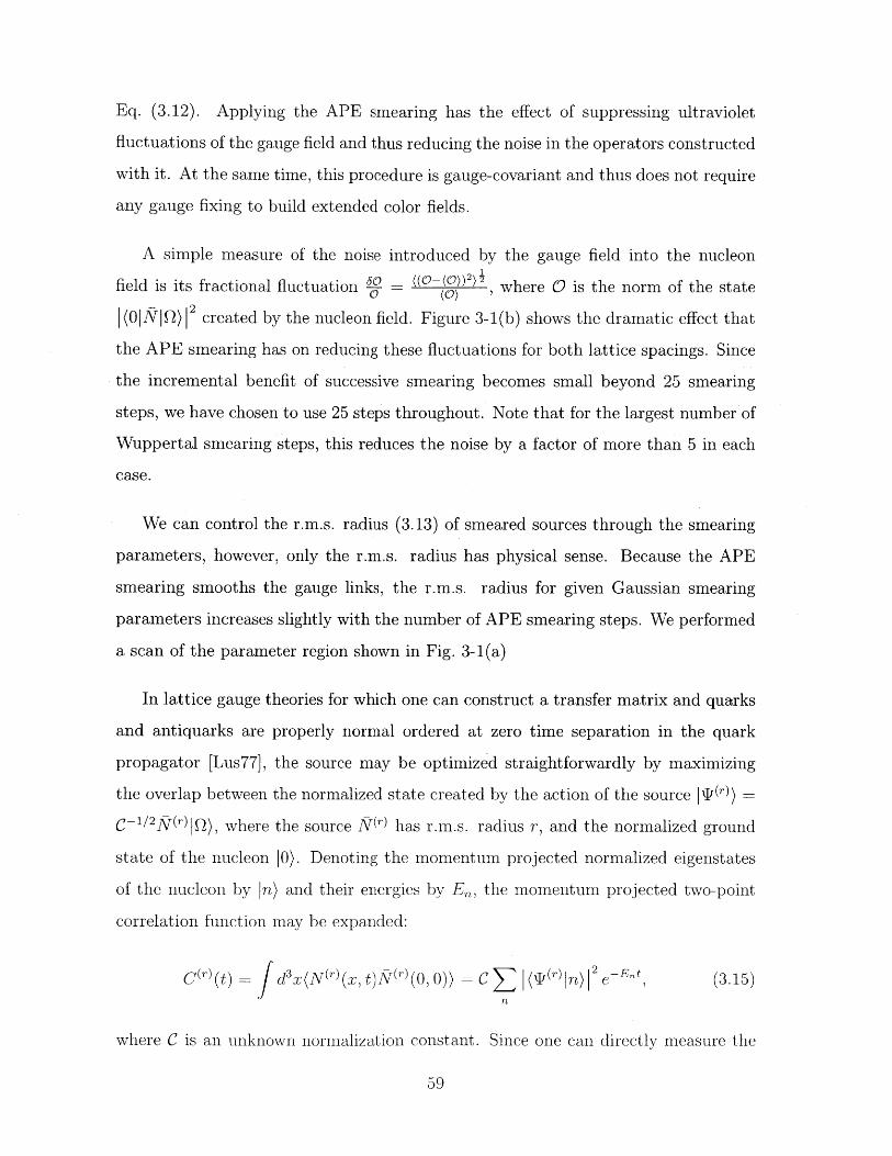
Eq. (3.12). Applying the APE smearing has the effect of suppressing ultraviolet
fluctuations of the gauge field and thus reducing the noise in the operators constructed
with it. At the same time, this procedure is gauge-covariant and thus does not require
any gauge fixing to build extended color fields.
A simple measure of the noise introduced by the gauge field into the nucleon
field is its fractional fluctuation (0) ,where 0 is the norm of the state
( OIIOQ) 2 created by the nucleon field. Figure 3-1(b) shows the dramatic effect that
the APE smearing has on reducing these fluctuations for both lattice spacings. Since
the incremental benefit of successive smearing becomes small beyond 25 smearing
steps, we have chosen to use 25 steps throughout. Note that for the largest number of
Wuppertal smearing steps, this reduces the noise by a factor of more than 5 in each
case.
We can control the r.m.s. radius (3.13) of smeared sources through the smearing
parameters, however, only the r.m.s. radius has physical sense. Because the APE
smearing smooths the gauge links, the r.m.s. radius for given Gaussian smearing
parameters increases slightly with the number of APE smearing steps. We performed
a scan of the parameter region shown in Fig. 3-1(a)
In lattice gauge theories for which one can construct a transfer matrix and quarks
and antiquarks are properly normal ordered at zero time separation in the quark
propagator [Lus77], the source may be optimized straightforwardly by maximizing
the overlap between the normalized state created by the action of the source |-O =
C- 1/ 2N(r)IQ), where the source N(r) has r.m.s. radius r, and the normalized ground
state of the nucleon |0). Denoting the momentum projected normalized eigenstates
of the nucleon by n) and their energies by En, the momentum projected two-point
correlation function may be expanded:
C (r)(t) d3 XKN(r)(x, t)N(r) (0, 0)) C L (rn) 2 ~E"' (3.15)n
where C is an unknown normalization constant. Since one can directly measure the
22
76
3210
800\ 30
40 0Wup. smearing steps 0
0 0 0 APE smearing steps(a) R.m.s radius (3.13) of Wuppertal-smeared (3.12) sources as a function of the coeffi-cient a = (4N/o,2 - 6)-1 and the number of smearing steps N
0/00.80.70.60.50.40.30.20.1
0
Wup. smearing
(b) Fractional variation of the nucleon state norm created with operator (3.11).
Figure 3-1: Scan of the Wuppertal and APE smearing parameter space.
correlation function at zero time separation
A(r) = C(r) (0) = C E (r) 2 ((3.16)
and reliably fit the large t behavior of the correlation function to extract the ground
state contribution
B) = C (q(r) |0) , (3.17)
the probability that the source contains the nucleon ground state may be calculated
by
p) B= = I |(r) 10) 2 (3.18)
For domain wall fermions, which do not have a local transfer matrix, we consider
the following generalization of Eqs. (3.16-3.18), which compares the ratio of the cor-
relation function and the extrapolated ground state contribution at time t instead of
time t = 0:
A(r)(t) C(r)(t), (3.19)
B (r(t) C |(4"|0) 2 , (3.20)
ip~) -BMr(t)p (t) A(r) . (3.21)A (r (t )
This ratio, P(r)(t), ranges from the overlap P(r) at t = 0 to 1 in the limit t -+ oc.
We expect that for small t, it is still a good measure of the presence of excited state
components in the source and should have a maximum close to the maximum in P(r).
This expectation is borne out in the case of Wilson fermions, and we note that this
criterion gets even better as the lattice spacing decreases. Since we are only interested
in the dependence of p)(t) on the r.m.s. radius r and the absolute normalization
for t $ 0 has no physical significance, it suffices to calculate the following ratio for
large toC(r)(to) to CI (r0)|2C-Eoto _ p(r)(t)E -t (3.22)C (t) C(r) (t)
For each value of t, it is convenient to normalize the curve such that its maximum
value is unity. Hence, defining the r.m.s. radius at the maximum as r*, our final
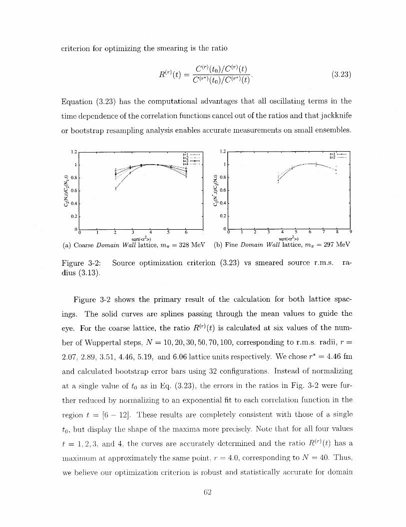
criterion for optimizing the smearing is the ratio
Cr) (to)/C(r)(t)R ((t) = to . (3.23)
Equation (3.23) has the computational advantages that all oscillating terms in the
time dependence of the correlation functions cancel out of the ratios and that jackknife
or bootstrap resampling analysis enables accurate measurements on small ensembles.
1.2 1.2t=2 t=1t 3
1 t=41
S0. 0.8
0.6 . 0.6
04-" 0.4 0.-
0.2 0.2
0 00 0 1 2 1' 4 5 6 7 8 9
sqrt(<r2>) sqrt(<r2 >)(a) Coarse Domain Wall lattice, m,= 328 MeV (b) Fine Domain Wall lattice, m, = 297 MeV
Figure 3-2: Source optimization criterion (3.23) vs smeared source r.m.s. ra-
dius (3.13).
Figure 3-2 shows the primary result of the calculation for both lattice spac-
ings. The solid curves are splines passing through the mean values to guide the
eye. For the coarse lattice, the ratio Rr)(t) is calculated at six values of the num-
ber of Wuppertal steps, N = 10, 20, 30, 50, 70, 100, corresponding to r.m.s. radii, r =
2.07, 2.89, 3.51, 4.46, 5.19, and 6.06 lattice units respectively. We chose r* = 4.46 fm
and calculated bootstrap error bars using 32 configurations. Instead of normalizing
at a single value of to as in Eq. (3.23), the errors in the ratios in Fig. 3-2 were fur-
ther reduced by normalizing to an exponential fit to each correlation function in the
region t = [6 - 12]. These results are completely consistent with those of a single
to, but display the shape of the maxima more precisely. Note that for all four values
t = 1, 2, 3, and 4, the curves are accurately determined and the ratio R(r)(t) has a
maximum at approximately the same point, r - 4.0, corresponding to N - 40. Thus,
we believe our optimization criterion is robust and statistically accurate for domain
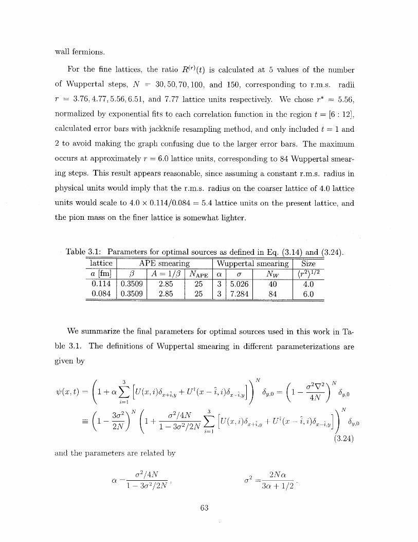
wall fermions.
For the fine lattices, the ratio R(r)(t) is calculated at 5 values of the number
of Wuppertal steps, N = 30, 50, 70, 100, and 150, corresponding to r.m.s. radii
r = 3.76, 4.77, 5.56, 6.51, and 7.77 lattice units respectively. We chose r* = 5.56,
normalized by exponential fits to each correlation function in the region t = [6 : 12],
calculated error bars with jackknife resampling method, and only included t =1 and
2 to avoid making the graph confusing due to the larger error bars. The maximum
occurs at approximately r - 6.0 lattice units, corresponding to 84 Wuppertal smear-
ing steps. This result appears reasonable, since assuming a constant r.m.s. radius in
physical units would imply that the r.m.s. radius on the coarser lattice of 4.0 lattice
units would scale to 4.0 x 0.114/0.084 = 5.4 lattice units on the present lattice, and
the pion mass on the finer lattice is somewhat lighter.
Table 3.1: Parameters for optimal sources as defined in Eq. (3.14) and (lattice APE smearing Wuppertal smearing Sizea [fm] # A = 1/0 NAPE a o- Nw (r2)120.114 0.3509 2.85 25 3 5.026 40 4.00.084 0.3509 2.85 25 3 7.284 84 6.0
3.24).
We summarize the final
ble 3.1. The definitions of
given by
parameters for optimal sources used in this work in Ta-
Wuppertal smearing in different parameterizations are
3 N-2 N2N N
+-1Y U) (x~ yO (1- 4N '
( 2 jN ( + 1 - 2 /4N Ujx, )6 + Ut](X - i, i6 N)I+ - 3u2 /21' -1,] '
(3.24)
and the parameters are related by
o-2 /4N1 - 3u2 /2N
2 2Na3 a + 1/2
3.1.3 Composite nucleon operators
In the conclusion of this section, we discuss a method to tune the nucleon interpolating
field [PS] that could potentially perform better than those discussed in Sec. 3.1.2. This
method is not used for calculations in the present work, however, it may be vital for
the future studies.
As pointed out after Eq. (3.11), its main disadvantage is that the quark wave
functions are independent. A simple way to improve this is to construct a "composite"
nucleon operator
N(x) = aiN (ii(A) (X) jj(Bi) (X), (Ci) (x)), (3.25)
where {A, B, C}2 denote the combinations of different types of spatial smearing of
the quark fields. Then, our goal is to tune the smearing combinations {A, B, C}2 and
their coefficients a so that the interpolating field creates a state which is orthogonal
to a number of the lowest excited states2
In principle, one can combine Gaussian smeared quarks (3.12) with different width
parameters. However, a series of Gaussian-smeared nucleon operators tends to create
states which are very close to being "collinear" in the Hilbert space. For example, if
the nucleon operators smeared with two different values o1 and Or2 create states
N1|I) A(IO) + ai l1)) + other exc. states, (3.26)N2| ) = B(10) + a 2|1)) + other exc. states,
with the main contamination given by the state 1) and a1 is close to a 2, the linear
combination of these states canceling the |1) state will be very noisy. Instead, one can
try adding node(s) to the quark wave functions used in Eq. (3.11) to create a different
superposition of 10) and |1) states and combine it with one of Eq. (3.26). Further, a
number of such operators constitutes a basis of states in which the orthogonalization
2 We emphasize that one has to suppress the excited states that are separated by the smallestgap from the ground state. The rest of the contamination will be suppressed by the evolutionfactor e-AEnot
procedure is more stable and reliable, especially when noisy lattice data are used for
source optimization.
For example, if some potential model is taken as a crude description of a nucleon,
the simplest form one may try is
N (x) = A N i(fO), fi(O), i(0))+B [N(6i), -() J 0 ))+N( ( 0 ,), 1), j(0))+N (6(4) GO), J)),
(3.27)
where 4(o) is the spherically-symmetric ground state wave function (without nodes)
of a quark in some model potential and 4(l) is the first excited state (with one node).
By tuning A and B one may obtain better overlap with the ground state than by
tuning the first term alone.
As a preliminary study, we compute an 8 x 8 two-point nucleon correlator matrix
(N(t)Nj(0)) corresponding to eight different nucleon operators at the source and the
sink using the BMW ensemble,
Ro = N (ft(0), ii(0), j(0))
N1 = N (6l), f(O), jC0))
N2 = N(( 0 ), gi(l), j(O)), (3.28)
N7 =N( , ),
where 0CO) is the Gaussian-smeared quark field (3.12) and 4() is the same profile with
the covariant Laplacian applied,
2
40() = A (1+ ' A)Nq] (x) (3.29)AN
Applying the Laplacian to the Gaussian distribution should produce a profile with a
node, as indicated by the free-field case
1'2 r 2 -3u02 r2
Ae 22 = r2 2-3 2
54
65
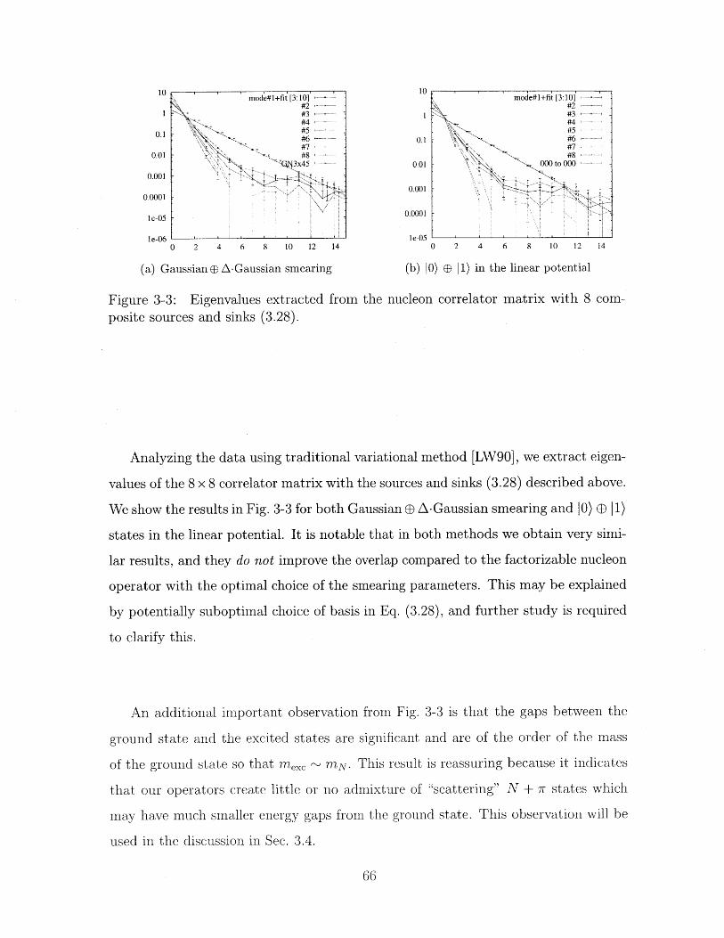
10 1mode#1+fit [3:10] - 10 mode#1+fit [3:10]
#2 #2#3 - 1#3#4 #4
0.1 #5 #5#6 -0.1 #6 -#7 #7
0.01 #8 #80.1 ij'~3x45 .00 \ ~ O~oO
0.001
0.0001 0.01 -
0.0001le-05
le-06 le-050 2 4 6 8 10 12 14 0 2 4 6 8 10 12 14
(a) Gaussian D A -Gaussian smearing (b) 10) e 1) in the linear potential
Figure 3-3: Eigenvalues extracted from the nucleon correlator matrix with 8 com-posite sources and sinks (3.28).
Analyzing the data using traditional variational method [LW90], we extract eigen-
values of the 8 x 8 correlator matrix with the sources and sinks (3.28) described above.
We show the results in Fig. 3-3 for both Gaussian e A-Gaussian smearing and 10) e 11)
states in the linear potential. It is notable that in both methods we obtain very simi-
lar results, and they do not improve the overlap compared to the factorizable nucleon
operator with the optimal choice of the smearing parameters. This may be explained
by potentially suboptimal choice of basis in Eq. (3.28), and further study is required
to clarify this.
An additional important observation from Fig. 3-3 is that the gaps between the
ground state and the excited states are significant and are of the order of the mass
of the ground state so that mexc ' mN. This result is reassuring because it indicates
that our operators create little or no admixture of "scattering" N + 7 states which
may have much smaller energy gaps from the ground state. This observation will be
used in the discussion in Sec. 3.4.
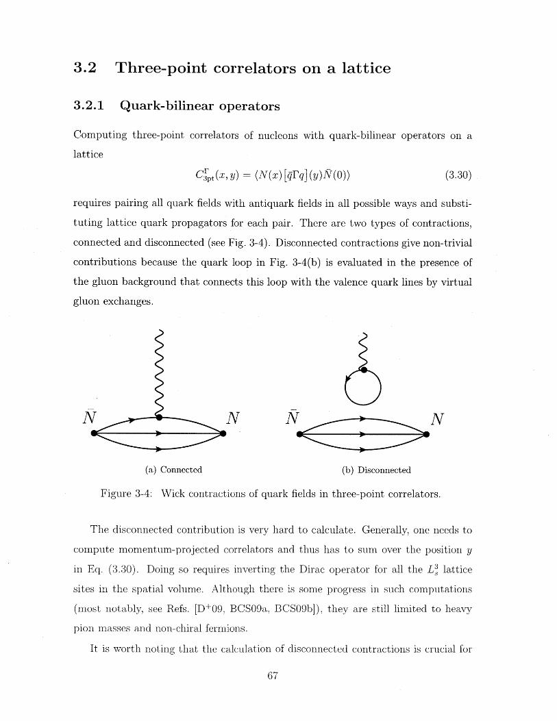
3.2 Three-point correlators on a lattice
3.2.1 Quark-bilinear operators
Computing three-point correlators of nucleons with quark-bilinear operators on a
lattice
C'(x, y) = (N(x) [qFq](y)N (0)) (3.30)
requires pairing all quark fields with antiquark fields in all possible ways and substi-
tuting lattice quark propagators for each pair. There are two types of contractions,
connected and disconnected (see Fig. 3-4). Disconnected contractions give non-trivial
contributions because the quark loop in Fig. 3-4(b) is evaluated in the presence of
the gluon background that connects this loop with the valence quark lines by virtual
gluon exchanges.
N N N N
(a) Connected (b) Disconnected
Figure 3-4: Wick contractions of quark fields in three-point correlators.
The disconnected contribution is very hard to calculate. Generally, one needs to
compute momentum-projected correlators and thus has to sum over the position y
in Eq. (3.30). Doing so requires inverting the Dirac operator for all the L3 lattice
sites in the spatial volume. Although there is some progress in such computations
(most notably, see Refs. [D+09, BCSO9a, BCSO9b]), they are still limited to heavy
pion iasses and non-chiral fermions.
It is worth noting that the calculation of disconnected contractions is crucial for
such problems as the strange quark content of the nucleon, quark spin contributions
to the nucleon spin and, in general, any isosinglet nucleon structure observables or
observables associated with one specific flavor. Computing connected contractions
gives the complete result only for flavor-nonsinglet contributions, for example, the
axial charge and the isovector form factors. However, even if advanced techniques
or resources to compute the disconnected contractions become available, one will
still have to reduce the noise in MC simulations and contaminations from excited
states. Therefore, in this work we focus mostly on isovector observables as a test case
to understand the precision that is possible to achieve, and lay the foundations for
complete nucleon structure calculations in the future.
3.2.2 Connected three-point quark correlators
In our calculations we use the so-called sequential source method [BDHS]. The se-
quential source method in this work is motivated by the same reason as in Ref. [H+08,
D+02]: it allows one to compute quark-bilinear operators with any Dirac matrix in-
sertion in Eq. (3.30) as well as covariant derivatives. However, when using the se-
quential source method, one has to fix the time locations of the nucleon source and
sink, thus making studying the systematic dependence on the source-sink separation
prohibitively expensive. Thus, a separate study of this potential source of systematic
effects is necessary, see Sec. 3.4.
Inversion of the Dirac operator on a lattice is a costly procedure, and, unless one
uses special stochastic estimator techniques [D+09], one can only compute a small
number of fermion propagators x <- y where y is a fixed point on a lattice:
01a(x, y) = (qa (xq(,3 (3.31)
In addition, one can use the so-called y5-hermiticity of Dirac operators, 73'$S - -
(the conjugation is applied to all the pairs of "indices", spin, color and coordinate),
to obtain the propagator x <- y where x is a fixed point:
[$[(x, y)] = 'Y [$ (y, X)Y5] ab (3.32)
Every lattice propagator (3.31) or (3.32) requires 12 inversions of the Dirac operator
7 on a lattice to compute all the combinations of spin and color indices.
The main idea of the sequential propagator method is to represent the three-point
correlator (3.30) as a trace of the product,
C3I4(x, y) = Trspin,color [SqNN(; X) (X, y') Fld(y', y) (y, 0)] (3.33)
where U(y, y') is the product of the gauge links along some path y -+ y' 3 and
SqNN (0; x) is the sequential source for the pair of a nucleon source and a sink at
points 0 and x, respectively. On a lattice, one successively computes the forward
propagator $1(9,0) ', the sequential source SNR(0; x), the backward propagator
SqN(0; x)$W(x, e) and, finally, the three-point function(s) (,y).
A sequential source SNN depends on a particular type of the nucleon interpolating
field, the source and sink locations, the nucleon polarization matrix, and the quark
flavor q. One may think of a sequential source as a two-point correlator with one of
the valence quark lines in Fig. 3-4(a) cut to insert an operator. Symbolically, one can
express a sequential source as
[SgNR(0; X)]" = IPO N6r (x) . g()R(0)) , (3.34)
where the angular brackets (( .)) denote (connected) contractions of the remaining
valence quarks. One usually computes three-point correlators with a momentum-
projected sink, summing S(0; x) over Y with an appropriate phase factor e',, and
3 These link paths allow one to construct the finite differences approximating covariant derivativeson a lattice. Computing the three-point correlators with the full set of link paths up to some length
("building blocks") was first used in Ref. [RenO4] and allows efficient computation of a number ofpoint-split quark-bilinear operators in a single run.
4 The dot "o" here and below denotes any point on the lattice. Thus, 01 (0, 0) is a lattice"vector" of fermion matrices.
using the fact that doing so commutes with the rest of the computation of three-point
functions.
If the nucleon interpolating fields are constructed from smeared quark fields one
has to apply the smearing kernel from Eq. (3.10)
" to both sides of the lattice quark propagators U and D, Q(x, y) -+ Q(x, y)
f dx' dy'K(x - x') Q(x', y')K(y' - y)
e and to the sequential source, S(0; x) -+ S(0; x) = f dx'S(0; x')K(x' - x).
Finally, to illustrate the sequential source method, we derive explicitly the ex-
pression for the sequential source S7 corresponding to the matrix element (ndfujp)
between proton and neutron states. Since we are working in the isospin limit, this
matrix element is equivalent to the (u - d) combination of the proton matrix elements,
Su = u S -S.(3.35)
This derivation is useful for calculations with so-called twisted boundary conditions
(TwBC) in which the spatial boundary conditions on a lattice are non-trivial and
different for the u and d quarks allowing one to have fractional (with respect to the
lattice momentum quantization) momentum transfer values Q2 -(P' - P)2.
We use the definition for the proton and neutron interpolating fields as
p=N(u,u,d), n=N(d,d,u). (3.36)
The variations of the proton and neutron fields with respect to the quark fields are
equal to
Sus -t n 6 a o E f3.-3 dfu
a/ f/ b/ C/12~' = Ec +±ocl1 do, un,,
Substituting the above expressions into Eq. (3.34) and using f, -y (1+_4 ),, 3 and
1+ PO' = FP 2 = , we get22
[ Qril3 o X 1 -a ]pPol ab'c' 6abc [ b D '
du1 (0 xf63,yj5 aa -o /a/ 16 f 16 ±a-y f+'&' [fa 5 ±o f0,]~a/b/c/'Eabc [FPO'/(SUl) bc (DS*)bc + S pl a'(D*)b
-(SUS*) a0(FPO1D) ±o (s oDS*)',a +±S)a0(P'S ~
where U = o=$ (x, 0) and D = (ddo) = .0 (x, 0).
We leave it to the reader to check that the relation (3.35) holds.
3.2.3 Composite sources
In this section we would like to summarize briefly the problems of computing three-
point functions with the composite sources discussed in Sec. 3.1.3. As we have de-
scribed in Sec. 3.2.2 one must plan carefully the order of computing quark propagators
and contracting them into two- and three-point correlators to maximize the useful
output of a calculation. Generally, with simple ("factorizable") sources one has to
compute one forward propagator and, separately, one backward propagator for each
flavor and sink position (or, equivalently, sink spatial momentum). The parity pro-
jection l-PY4 further reduces the number of inversions by a factor of two.
However, if one constructs a nucleon state with a composite nucleon operator,
each term in Eq. (3.25) requires the calculation of a separate full set of inversions
and contractions multiplying the cost by an integer factor. It is remarkable that the
composite nucleon sink does not require additional computations except for smearing
and computing contractions in the sequential sources Sq.
Thus, the most effective strategy is to use a composite nucleon sink and a simple
nucleon source. Unfortunately, such approach will result in asymmetric plateaus even
for forward matrix elements which are usually the "gold-plated" quantities computed
on a lattice. One needs to implement a convoluted fitting procedure to extract nucleon
matrix elements from such plateaus that takes into account the fact that the data
points closer to the sink are more credible than those closer to the source.
In practice, however, calculations with an asymmetric source-sink pair may be
the only reasonable choice to study the nucleon form factors at non-zero momentum
transfer. According to the recent study in Ref. [LCE+10], optimal source parameters
may depend on the momentum of a nucleon state. However, in the present calculations
momentum projection is performed for sink and operator locations while the position
of a source is fixed and thus contains all possible momenta. Hence, it is impossible
to tune both the source and the sink to suppress the most dangerous excited states.
Instead, tuning of the sink can be performed at each sink momentum separately with
negligible additional cost required for separate smearing of quark propagators.
3.3 Form Factors
3.3.1 Transfer matrix expressions
In order to calculate nucleon matrix elements, we compute the three-point polarized
nucleon correlators involving the vector current, along with the two-point correlators
[H+08):
C2 pt(t, P) = e~ (Fpoi). (Ng (2, t)Na(0 , 0)), (3.37)
x o
(3.38)
where N, N, are the lattice nucleon operators; (| NQ(x)I P, o) = \Z(P)USY (P)ewith Z(P) parameterizing the overlap with the nucleon ground state; (P0, 1)C'O
2 1 ~ is the spin and parity projection matrix5 ; and 0 is the operator in ques-
5 In this subsection, we use Euclidean 7-matrices, (7i)t = -y4, { =4, "} =26".
tion. In the transfer matrix formalism, these correlators take the form
C2 ~(t,) -Z(P)e-Et
C2pt(tip) = 2E Tr [Fpoi (i4 + MN)] + excited states, (3.39)
C (P - Z (P ) .Z (P )e E'(T -r)-ErCpt (Ti T; P, P')=x
2E'- 2E
x Tr Kpoi (ip ' + MN) P P) ( MN) (3.40)
+ excited states,
where E and E' are the ground state energies of the initial and final nucleon states
and F (P', P) is the vertex corresponding to an operator 0,
(N(P', S')10(0)1N(P, S)) = U(P', S')F(P', P)U(P, S), (3.41)
which is parameterized with corresponding form factors, e.g. Dirac and Pauli form
factors for the electromagnetic current operator. Excited state contributions have
generally similar forms with different Z-factors, vertices and higher energies Eexc > E.
The systematic effects related to them will be discussed in Sec. 3.4.
Equations (3.39,3.40) describe the evolution of an on-shell particle with energy
E = P 2 + My with the Euclidean time. After the Wick rotation, the Euclidean
4-momentum P must have an imaginary time component, resulting in
PEuc = (, -iE) (j, - p2 + MN). (3.42)
Note that the polarization matrix (iP + MN) constructed with Euclidean 7-matrices (3.43)
directly corresponds to the polarization matrix (P Mink + MN) constructed from Minkowski
4-momentum and 7-matrices,
(7,,)Euc _ -. 1,2,3 Mink, (- )Euc _ ( 4 Mink , (75Euc =-f 1 )a (1234Euc 5)Mink
(3.43).pEuc =( pEuc7 EUc) -'Mn F>)ik (' 0
-jMink . 5 Mlink) (34
3.3.2 Nucleon matrix elements
In order to extract nucleon matrix elements (3.41) we combine lattice nucleon cor-
relators (3.39, 3.40) into the usual ratio of three- and two-point correlation func-
tions [H+08], which we find useful to write in a convenient and illuminating new form
as follows. First, we define two ratios, a normalization ratio, RN, and an asymmetry
ratio, RA,
Cpt(T, T; P, P')
VC2pt (T, P) C2pt (T, P'
RN C2pt(T - r, P)C2pt (T, P') (3.46)FC2p t (T - r, P')C2pt (7, P)
The physical matrix element is then given by the product
C-9pt(T, T; P, P') C2pt(T - r, P)C 2pt(T, P')
RC2pt(T P) C2pt(T P') C2pt (T - T, P')C 2pt (T, P) (3.47){T, r, T-r}-*oo ZSS' (UpP S)FPolU(P', S')) - (P', S' 0 P, S)
2E (E±+ MN ) -2E'( E'±+ MN )
The normalization ratio RN has the property that all the lattice-dependent overlap
factors Z for the ground state cancel out, which motivates its name, and in the case
of forward matrix elements P = P' it yields the final result for the corresponding
matrix element. The asymmetry ratio RA compensates the asymmetric exponential
T dependence of the three-point correlator, thus motivating its name. In the absence
of excited states, it would be equal to exp [-(E' - E)(r - T/2)] and in the forward
case, P' P, this ratio is trivial and equal to one, RA(T) ,s 1. In the general
case, P' -f P, this ratio is still identically one in the center of the plateau, r T/2,
and by construction possesses the following symmetry around the plateau center:
RA(T - T) = 1/RA(r).
The limits {T, -r, T - r} - oc should be taken to get rid of excited state con-
taminations. In practice, this requires adopting a value of source-sink separation T
large enough so that the excited state contributions to Eq. (3.47) are negligible com-
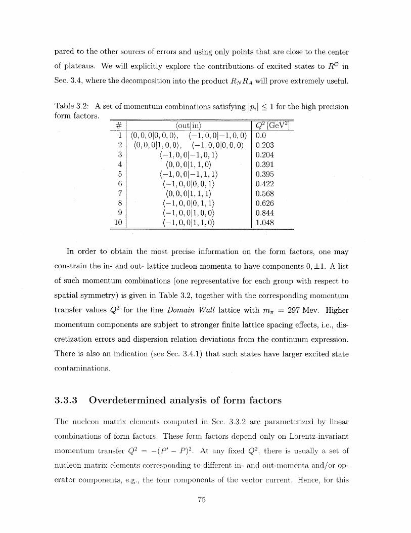
pared to the other sources of errors and using only points that are close to the center
of plateaus. We will explicitly explore the contributions of excited states to R0 in
Sec. 3.4, where the decomposition into the product RNRA will prove extremely useful.
Table 3.2: A set of momentum combinations satisfying 1pi < 1 for the high precisionform factors.
# (outlin) Q2 [GeV2 )1 (0,0 000, 0,0, 0) (-1, 0, 0|-1, 0, 0) 0.02 (0, 0, 011, 0, 0), (-1, 0, 010, 0, 0) 0.2033 (-1, 0, 0|-1, 0, 1) 0.2044 (0, 0, 0|1, 1, 0) 0.3915 (-1, 0, 0|-1, 1, 1) 0.3956 (-1,, 000, 0, 1) 0.4227 (0, 0,1 011, 1) 0.5688 (-1,0 000, 1, 1) 0.6269 (-1, 0, 0|1, 0, 0) 0.844
10 (-1, 0, 0|1, 1, 0) 1.048
In order to obtain the most precise information on the form factors, one may
constrain the in- and out- lattice nucleon momenta to have components 0, ±1. A list
of such momentum combinations (one representative for each group with respect to
spatial symmetry) is given in Table 3.2, together with the corresponding momentum
transfer values Q2 for the fine Domain Wall lattice with m, = 297 Mev. Higher
momentum components are subject to stronger finite lattice spacing effects, i.e., dis-
cretization errors and dispersion relation deviations from the continuum expression.
There is also an indication (see Sec. 3.4.1) that such states have larger excited state
contaminations.
3.3.3 Overdetermined analysis of form factors
The nucleon matrix elements computed in Sec. 3.3.2 are parameterized by linear
combinations of form factors. These form factors depend only on Lorentz-invariant
momentum transfer Q2 (B'_ p )2 . At any fixed Q2, there is usually a set of
nucleon matrix elements corresponding to different in- and out-momenta and/or op-
erator components, e.g., the four components of the vector current. Hence, for this
usual case of multiple matrix elements, one can extract form factor values by solving
an overdetermined system of equations. This is best demonstrated with the vector
current form factors, Dirac F1 and Pauli F2 ,
l'" (P', P) =1(Q 2) 2MNI' q F( -2 -q (3.48)
Transforming the above expression to Euclidean space and substituting it into Eq. (3.40)
and then Eq. (3.47) and neglecting the excited states, we obtain an overdetermined
system of equations for the form factors F1,2(Q2):
Aa1 F1 + Aa 2 F2 - Ru', (3.49)
where a is a composite index specifying the component of the current, "P", and the
initial and final nucleon momenta. The right-hand side in Eq. (3.49), R., is a set of
matrix elements evaluated using Eq. (3.47) from nucleon correlators computed on a
lattice.
We find the solution of the overdetermined system (3.49) from a linear fit, which
minimizes the functional
F = E (AnjF - R,))C-1 (A,, F. - Rl), (3.50)
where C,, is the estimation of the covariance matrix of R0 ,
1CGo3 - (((RKRR)) - ((Ra))K(R))), (3.51)
N - 1
with the double brackets denoting an ensemble average. Using the covariance matrix
is crucial because the lattice correlation functions are often correlated.
Since the estimated covariance matrix may be ill-determined, it can introduce
uncontrollable errors into the extracted form factors. In general, a covariance matrix is
notoriously difficult to estimate reliably in statistical analyses. To make sure the linear
fitting gives correct result, we repeat the analysis with only the diagonal elements of
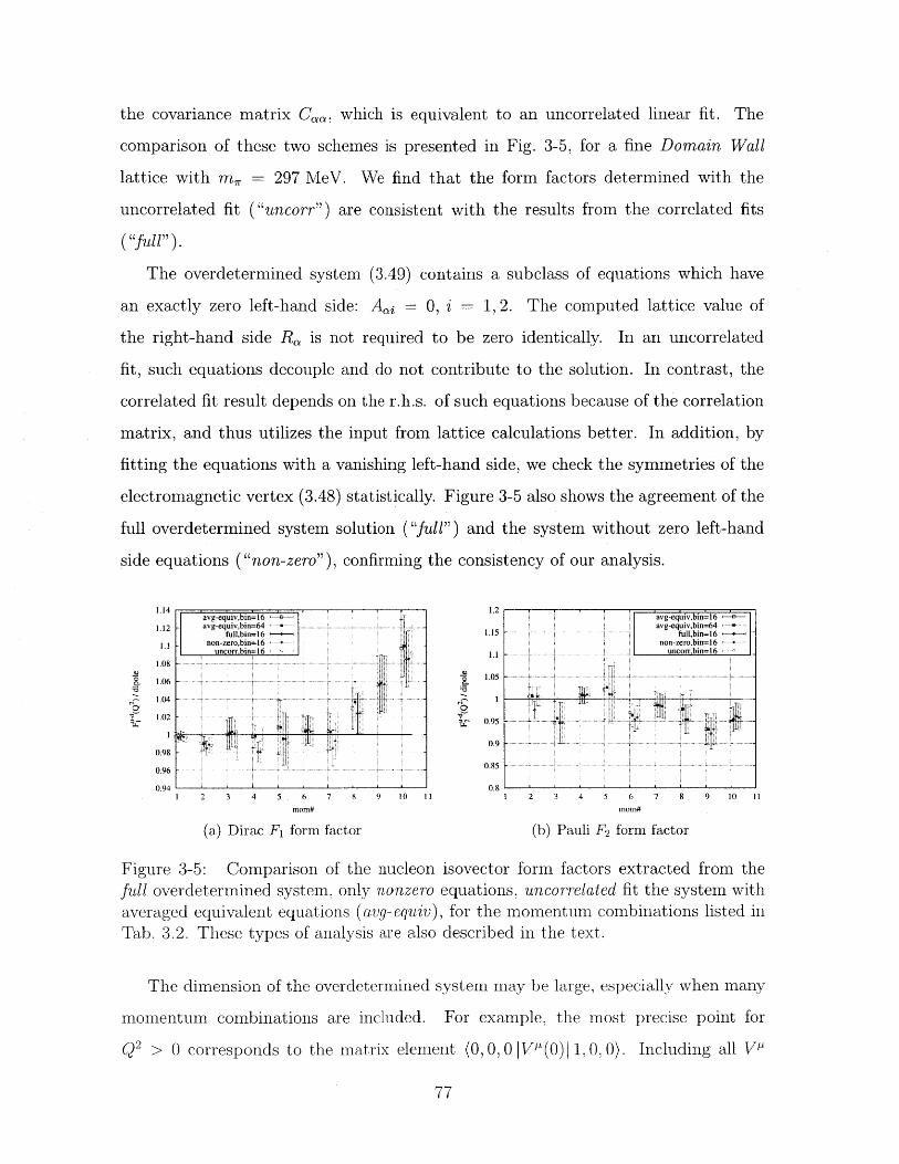
the covariance matrix C,,, which is equivalent to an uncorrelated linear fit. The
comparison of these two schemes is presented in Fig. 3-5, for a fine Domain Wall
lattice with m, = 297 MeV. We find that the form factors determined with the
uncorrelated fit ("uncorr") are consistent with the results from the correlated fits
(C"full" ).
The overdetermined system (3.49) contains a subclass of equations which have
an exactly zero left-hand side: A0 j = 0, i = 1, 2. The computed lattice value of
the right-hand side RQ is not required to be zero identically. In an uncorrelated
fit, such equations decouple and do not contribute to the solution. In contrast, the
correlated fit result depends on the r.h.s. of such equations because of the correlation
matrix, and thus utilizes the input from lattice calculations better. In addition, by
fitting the equations with a vanishing left-hand side, we check the symmetries of the
electromagnetic vertex (3.48) statistically. Figure 3-5 also shows the agreement of the
full overdetermined system solution ("full") and the system without zero left-hand
side equations ("non-zero"), confirming the consistency of our analysis.
1.14 1.2avg-egmyvbm=16 avg-equivbin=16
1.12 avg-equiv, bin 65 - avg-equiv bin=64full bin=16 1.15 full bin- 16
1.1 non-zero bin-16 non zero bin=16 -uncorr bin=16 11ncorrbin=16
1.08
1.06 - 1.05
1.04.1.020.95
g.T *0.9 -0.98
0.96 -. 0.85
0.94 0.81 2 3 4 5 6 7 8 9 10 11 1 2 3 4 5 6 7 8 9 10 11
mom# mom#
(a) Dirac F form factor (b) Pauli F2 form factor
Figure 3-5: Comparison of the nucleon isovector form factors extracted from thefull overdetermined system, only nonzero equations, uncorrelated fit the system withaveraged equivalent equations (avg-equiv), for the momentum combinations listed inTab. 3.2. These types of analysis are also described in the text.
The dimension of the overdetermined system may be large, especially when many
momentum combinations are included. For example, the most precise point for
Q2 > 0 corresponds to the matrix element (0, 0, 0| V(0) 1,0 0). Including all VP
components, together with spatial rotations and reflections gives 48 equations, only
16 of which are nonzero. It is useful to combine all the nucleon matrix elements for
each fixed Q2 into equivalence classes based on the spatial (rotational and reflection)
symmetry. We adopted the following heuristic equivalence criteria 6 for three-point
functions:
1. The momenta of in- and out-states must be equivalent under the spatial sym-
metry.
2. The corresponding coefficients Aj in Eq. (3.49) must be equal up to an overall
sign.
3. The components of the current operator must be both temporal or both spatial
and both real or both imaginary parts of a matrix element.
Blocking the three-point correlators within equivalence classes is advantageous for
two reasons. First, this reduces the dimension of the system of equations (3.49) and
the covariance matrix we need to estimate, and we note that blocking strongly corre-
lated values improves the covariance matrix condition number. Second, we may block
the three- and two-point correlators separately before computing the ratio (3.47). Do-
ing so improves the ratio method in Eq. (3.47) by reducing the fluctuations of the
denominator because of the two-point correlators. We compare the form factor ex-
traction results using this method ("avg-equiv") to other methods in Fig. 3-5 and find
that this averaging does not introduce any systematic errors.
The main method we use to extract the final set of the form factors is the correlated
fit to the reduced (i.e., the system with no equations whose left-hand side is zero)
overdetermined system with blocked equivalent equations.
6 We did not classify the matrix elements according to the hypercubic lattice symmetry. Insteadwe use the relations derived in the continuum theory. Thus these criteria may be thought of asnumerical means to improve the condition number of a linear system we need to solve.
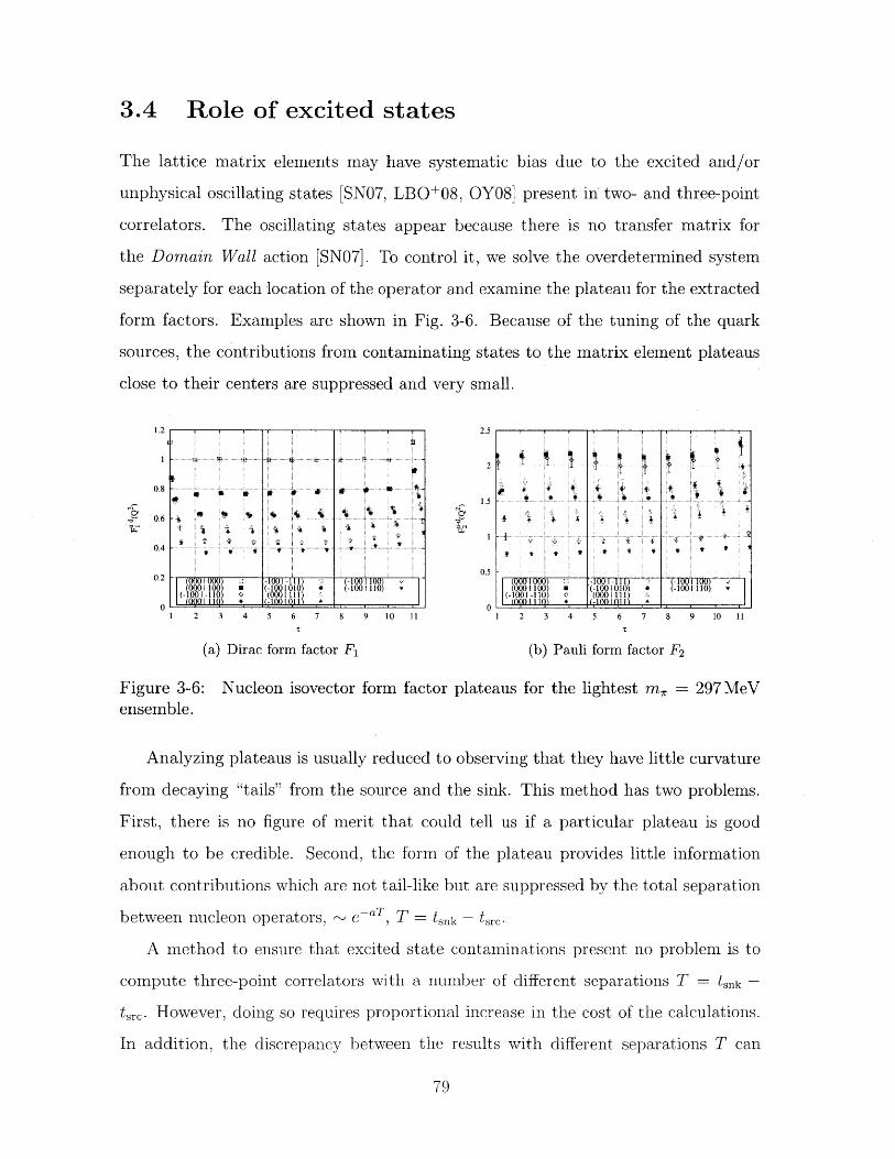
3.4 Role of excited states
The lattice matrix elements may have systematic bias due to the excited and/or
unphysical oscillating states [SN07, LBO+08, OY08] present in' two- and three-point
correlators. The oscillating states appear because there is no transfer matrix for
the Domain Wall action [SN07]. To control it, we solve the overdetermined system
separately for each location of the operator and examine the plateau for the extracted
form factors. Examples are shown in Fig. 3-6. Because of the tuning of the quark
sources, the contributions from contaminating states to the matrix element plateaus
close to their centers are suppressed and very small.
1.2 I 1 1 I i2.5
1
0.8
-~0.6
0.4
0.2
01
... .......* .- .......# V
.. .... . ..... ..... ....
01 1 10 1011 ~71 2 3 4 5 6 7 8 9 10 11 1 2 3 4 5 6 7 8 9 10 11
T T
(a) Dirac form factor F (b) Pauli form factor F2
Figure 3-6: Nucleon isovector form factor plateaus for the lightest m, = 297MeVensemble.
Analyzing plateaus is usually reduced to observing that they have little curvature
from decaying "tails" from the source and the sink. This method has two problems.
First, there is no figure of merit that could tell us if a particular plateau is good
enough to be credible. Second, the form of the plateau provides little information
about contributions which are not tail-like but are suppressed by the total separation
between nucleon operators, ~ e--"T, T =ts k - tsrc.
A method to ensure that excited state contaminations present no problem is to
compute three-point correlators with a number of different separations T= tsnk -
tsrc. However, doing so requires proportional increase in the cost of the calculations.
In addition, the discrepancy between the results with different separations T can
1100 a (-1001010 :10 a0
F- -a 10 1 1-Q 1'1
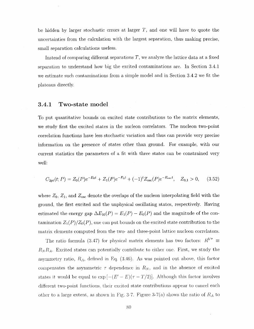
be hidden by larger stochastic errors at larger T, and one will have to quote the
uncertainties from the calculation with the largest separation, thus making precise,
small separation calculations useless.
Instead of comparing different separations T, we analyze the lattice data at a fixed
separation to understand how big the excited contaminations are. In Section 3.4.1
we estimate such contaminations from a simple model and in Section 3.4.2 we fit the
plateaus directly.
3.4.1 Two-state model
To put quantitative bounds on excited state contributions to the matrix elements,
we study first the excited states in the nucleon correlators. The nucleon two-point
correlation functions have less stochastic variation and thus can provide very precise
information on the presence of states other than ground. For example, with our
current statistics the parameters of a fit with three states can be constrained very
well:
C2p (t; P) = Zo(P)eEot i+ Z(P)eElt + (1)tZosc(P)e-Eosct, Zo,1 > 0, (3.52)
where Z0 , Z 1, and Zscs denote the overlaps of the nucleon interpolating field with the
ground, the first excited and the unphysical oscillating states, respectively. Having
estimated the energy gap AEio(P) = E1 (P) - Eo(P) and the magnitude of the con-
tamination Z 1(P)/Zo(P), one can put bounds on the excited state contribution to the
matrix elements computed from the two- and three-point lattice nucleon correlators.
The ratio formula (3.47) for physical matrix elements has two factors: RVP -
RNRA. Excited states can potentially contribute to either one. First, we study the
asymmetry ratio, RA, defined in Eq. (3.46). As was pointed out above, this factor
compensates the asymmetric T dependence in RN, and in the absence of excited
states it would be equal to exp [-(E' - E)(r - T/2)]. Although this factor involves
different two-point functions, their excited state contributions appear to cancel each
other to a large extent, as shown in Fig. 3-7. Figure 3-7(a) shows the ratio of RA to
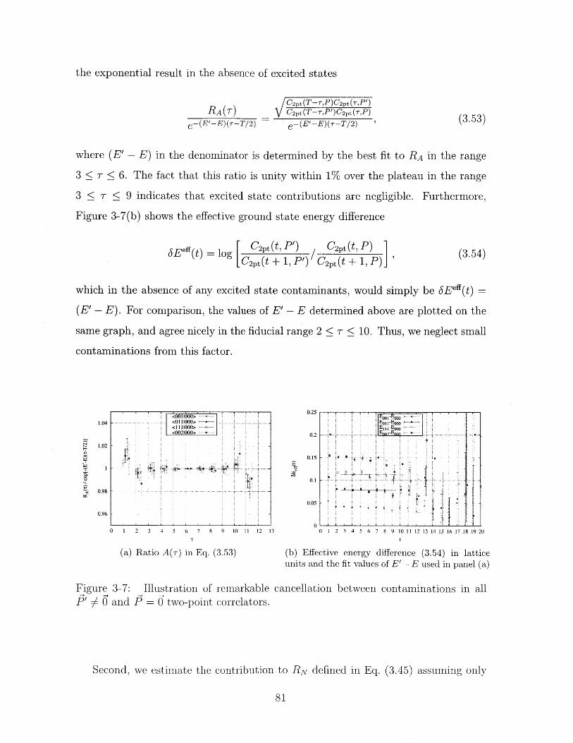
the exponential result in the absence of excited states
RA(T)
-(E'-E)(r -T/2)
C2pt (T-rP)C2pt (-r,P')C2pt(T-/,P)c2pt(,P)
-(E'-E)(-r-T/2) ,
where (E' - E) in the denominator is determined by the best fit to RA in the range
3 < r < 6. The fact that this ratio is unity within 1% over the plateau in the range
3 < T < 9 indicates that excited state contributions are negligible.
Figure 3-7(b) shows the effective ground state energy difference
Furthermore,
JE eff~(t) log C2pt (t, P') C2pt (t, F) ]_ C2pt(t + 1, P') C2pt(t + 1, P)
(3.54)
which in the absence of any excited state contaminants, would simply be 6E*ff(t) =
(E' - E). For comparison, the values of E' - E determined above are plotted on the
same graph, and agree nicely in the fiducial range 2 < T < 10. Thus, we neglect small
contaminations from this factor.
<001100>
<1111000><0021000>
... ......
0 1 2 3 4 5 6 7 8 9 10 11 12 13
(a) Ratio A(r) in Eq. (3.53)
0.25
0.2 --
0.15
0.05
00 1 2 3 4 5 6 7 8 9 10 11 12 13 14 15 16 17 18 19 20
t
(b) Effective energy difference (3.54) in latticeunits and the fit values of E'- E used in panel (a)
Figure 3-7:j' f 0 and
Illustration of remarkableP = 0 two-point correlators.
cancellation between contaminations in all
Second, we estimate the contribution to RN defined in Eq. (3.45) assuming only
(3.53)
one excited state and no oscillating term7 :
C3pt(rT) C3pt(, (T + e-AEr Z{' -AE'(T-)
p 1 0 0010 rZ 0II
Z1Z 1 01'1 -AE'(T-r)-AEr
Z 0ZO 0 010 e
C3pt (T, T) C 3pt (T, T) x1 rR (90 xi 1+ (" 6R'O (T -T)
C2 pt~, (T) Cp, (T) C2pt (T) C2pt (T) ' o' 0
0 - 1+ 0 Rio(T)R'O(T - T) -(6R + 6R')-
00,0 2
(3.55)
where
6R(') (r) e -AE(')r
0
Z(') -AE(')T - [3R( 2 (3.56)
and we have expanded Eq. (3.45) assuming that 6R(' < 1. The value of the suppres-
sion factor SR(')(r) is shown in Fig. 3-8. Its values are estimated using parameters
Zo, 1, E1,0 from the fit using Eq. (3.52), and the errors are computed using the jack-
knife procedure. It is remarkable that 6R(')(T) falls off steeply with T. As a result,
its contribution can be easily detected and removed by fitting the plateau with
R0 ,r) Co + C1 e-AEr + C -AE'(T--r) (3.57)
From Fig. 3-8 one may estimate the last two terms in the contamination formula (3.55),
suppressed by 6R(' and 6Rio(r)OR'O(T - T). If one assumes further that the excited
state matrix elements are at most of the same order as the ground state matrix el-
ements, ':", < 1, the effect of the last two terms in Eq. (3.55) is well below 1%. It
is also worth noting that higher momentum matrix elements with p = (0, 0, 2) may
contain substantially larger contamination, as compared to lower momentum matrix
7 We neglect the contribution of oscillating states because they decay even faster than excited
states.
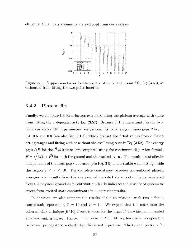
elements. Such matrix elements are excluded from our analysis.
0.1 -
0.01 -
p=(O,O,O) 1p=(O0,I,)
0.0010 1 2 3 4 5 6 7 8 9 10 11 12 13 14
Figure 3-8: Suppression factor for the excited state contributions 6Rio(T) (3.56), asestimated from fitting the two-point function.
3.4.2 Plateau fits
Finally, we compare the form factors extracted using the plateau average with those
from fitting the T dependence to Eq. (3.57). Because of the uncertainty in the two-
point correlator fitting parameters, we perform fits for a range of mass gaps AMN
0.4, 0.6 and 0.8 (see also Sec. 3.1.3), which bracket the fitted values from different
fitting ranges and fitting with or without the oscillating term in Eq. (3.52). The energy
gaps AE for the P # 0 states are computed using the continuum dispersion formula
E = MN + P2 for both the ground and the excited states. The result is statistically
independent of the mass gap value used (see Fig. 3-9) and is stable when fitting inside
the region 2 < T < 10. The complete consistency between conventional plateau
averages and results from the analysis with excited state contaminants separated
from the physical ground state contribution clearly indicates the absence of systematic
errors from excited state contaminants in our present results.
In addition, we also compare the results of the calculations with two different
source-sink separations, T = 12 and T - 14. We expect that the noise from the
coherent sink technique [B+ 101, if any, is worse for the larger T, for which an unwanted
adjacent sink is closer. Hence, in the case of T = 14, we have used independent
backward propagators to check that this is not a problem. The typical plateaus for
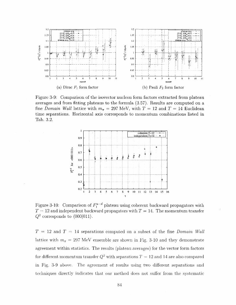
plateau avg[3:9], AMN=0.
4
[3-91,AMN=O06[3:9], AM -08
plateau avg=14
IT i, T:
1 2 3 4 5 6 7 8 9 10 11mom#
(a) Dirac F form factor
2 3 4 5 6 7 8 9 10 11mom#
(b) Pauli F2 form factor
Figure 3-9: Comparison of the isovector nucleon form factors extracted from plateauaverages and from fitting plateausfine Domain Wall lattice with m,
to the formula (3.57). Results are computed on a= 297 MeV, with T = 12 and T = 14 Euclidean
time separations. Horizontal axis corresponds to momentum combinations listed inTab. 3.2.
0.8
0.7
0.6
0.5
0.4
1 2 3 4 5 6 7 8 9 10 11 12 13 14 15 16
Figure 3-10: Comparison of F d plateau using coherent backward propagators withT = 12 and independent backward propagators with T = 14. The momentum transferQ2 corresponds to (000|011).
T 12 and T = 14 separations computed on a subset of the fine Domain Wall
lattice with m, = 297 MeV ensemble are shown in Fig. 3-10 and they demonstrate
agreement within statistics. The results (plateau averages) for the vector form factors
for different momentum transfer Q2 with separations T
in Fig. 3-9 above.
12 and 14 are also compared
The agreement of results using two different separations and
techniques directly indicates that our method does not suffer from the systematic
84
coherent,T=12independent,T= 14+
I I I I I i i I i I
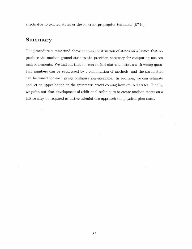
effects due to excited states or the coherent propagator technique [B+10].
Summary
The procedure summarized above enables construction of states on a lattice that re-
produce the nucleon ground state to the precision necessary for computing nucleon
matrix elements. We find out that nucleon excited states and states with wrong quan-
tum numbers can be suppressed by a combination of methods, and the parameters
can be tuned for each gauge configuration ensemble. In addition, we can estimate
and set an upper bound on the systematic errors coming from excited states. Finally,
we point out that development of additional techniques to create nucleon states on a
lattice may be required as lattice calculations approach the physical pion mass.

86
Chapter 4
Renormalization of Lattice
Quark-Bilinear Operators
In this section we discuss how the nucleon structure observables calculated on a lat-
tice should be renormalized before comparing with experimental results. Generally,
it requires matching between lattice and continuum calculations quark correlators.
In Section 4.1 we discuss some general aspects of renormalization of lattice observ-
ables. We mention briefly the renormalization using lattice perturbation theory in
Sec. 4.1.1, and proceed to the nonperturbative renormalization methods in Sec. 4.2,
which is used as the main method in this work. We present the details of match-
ing between continuum and lattice observables in Section 4.3, and analyze possible
sources of systematic bias arising from this matching. The final numbers for lattice
renormalization coefficients are collected in Appendix C.
4.1 General aspects of renormalization
4.1.1 Linking lattice calculations and experiment
Lattice QCD is a gauge theory regularized by the introduction of a space-time lattice,
making path integrals finite-dimensional. Generally an operator constructed on a
lattice requires renormalization since their computed matrix elements are bare values
with fixed ultraviolet cutoff determined by the inverse lattice spacing At = a- 1. To
make comparisons to experimental values possible, one has to convert these values to
an appropriate renormalization scheme, which is usually the MS scheme at the scale
p2 = (2GeV) 2 widely used in phenomenology.
One possible approach to this problem is to compare perturbative calculations in
lattice and continuum theories. While the perturbation theory in continuum QCD
is well-developed and boasts calculations up to four loops, the perturbative compu-
tations in lattice QCD are much more complex. So far, most of lattice perturbative
calculations are limited to one loop. This limitation is especially bad because one
usually has a rather small ultraviolet cutoff; current lattice simulations are performed
with lattice spacing values a- 1 < 4 GeV. One might worry that the strong coupling
o's at this scale is large, and the convergence of lattice perturbation calculations is
expected to be slow, invalidating one-loop calculations. In addition, it is very hard
to estimate the systematic effects due to perturbative series truncation [B+10].
The convergence of perturbative renormalization factors may be improved by the
tadpole improvement of perturbation theory [LM93]. For example, the one-loop per-
turbative renormalization factors were computed for mixed action calculations [Bis05].
Below in this chapter we will compare the calculation in Ref. [Bis05] to the nonper-
turbative calculation (see Sec. 4.4).
4.1.2 Mixing of lattice operators
Under renormalization, different lattice operators can mix with each other. In this
section we discuss what consequences this mixing may have for our calculations and
how it can be avoided.
Firstly, there is physical mixing between flavor-singlet quark and gluon contribu-
tions to the nucleon structure observables, e.g., nucleon momentum, angular momen-
tum and structure functions. In the DGLAP evolution equations this corresponds
to the mixing of quark and gluon distribution functions, if the former are not pro-
tected by conservation laws'. For proper renormalization of the quark contribution
' This is not the case for the isovector components, e.g. u(x) - d(x) which is protected by the
to the nucleon structure the gluon counterpart which mixes with it must also be
computed. However, because of the stochastic noise associated with fluctuations in
the gluon field, the gluon contributions requires roughly the same computational re-
sources as disconnected diagrams and therefore have been neglected in this work.
Therefore, presently we have to neglect the mixing of quark and gluon observables.
The uncertainty because of quark-gluon mixing is relevant only to isosinglet quark
observables. Since the isosinglet channel has also uncertainty from the disconnected
contractions (see Sec. 3.2), we find it useful to concentrate on isovector observables,
which do not have such complications, and treat the results for isoscalar observables
as approximate.
Secondly, the lattice regularization reduces the rotational symmetry, as was dis-
cussed in Sec. 2.4. This results in irreducible "spin" representations of SO(4) breaking
up into a finite number of representations of the hypercubic group H(4) [G+96a]. If
operators of different spins and/or dimensions have components in the same H(4)
representation they can mix; this mixing is unphysical and a pure lattice artifact.
In our study, we compute the matrix elements of twist-2 operators, which are the
series of operators with growing dimension and spin. In the continuum, these op-
erators are protected from mixing because they belong- to different representations
of SO(4). On a lattice, however, the number of representations of the lattice "rota-
tion group" H(4) is finite, and the higher-dimensional operators will imminently mix
with lower-dimensional operators. The mixing coefficient is necessarily dimensionful
and determined by the lattice cutoff Aat = a- 1 and it diverges in the continuum
limit [BBCR95, G+96b] prohibiting reliable calculation of higher-dimensional oper-
ators on a lattice [G+96a]. Practically, we are limited to computing the twist-2
operators up to dimension d = 6. For the operators with d < 6 we have to choose
carefully the H(4) representations to avoid mixing [D+02, H+03].
In principle, it is possible to find the mixing coefficients nonperturbatively and
subtract the lower-dimensional contributions as was done in Ref. [G+05a].
isospin conservation.
4.1.3 Special cases of lattice renormalization
In some special cases the renormalization of lattice operators is not required or is
very simple. For example, in the computation of vector form factors one can use
the forward value of the Dirac form factor as the renormalization factor. Because
the vector current is conserved, the total charge gv = Fen(0) is determined by the
number of valence quarks. Thus, renormalizing the vector current gy Iq is trivial:
(N|sN = Fva ) (N I [q-y" q] atN), (4.1)
where Qvai is the total charge of the valence quarks in the state |N). Although we
say that the vector current is conserved, its particular lattice representation may
still have multiplicative renormalization. There is, of course, the true conserved
current generated by the U(1)v symmetry of the action, but it usually involves fermion
fields from several lattice sites, i.e., it is not site-local, and it is inconvenient for
numerical reasons. Instead of it, one usually employs the site-local current $274#
and renormalizes it with Eq. (4.1).
In the case of Wilson(-Clover) fermions, the conserved current has the form
Vwilson + ___U_' -2 #+ (4.2)
for which one may directly check using the equations of motion for 7P following from
Wilson(-Clover) action (2.19,2.20) that its divergence is zero,
(V -V,) =3 [Vxl - V2 ,,] = 0, [eqn. of motion] (4.3)
and the correlators with this current operator satisfy the corresponding Ward identity.
Using the Ward identity for the conserved current, one can show that Zv = 1 in the
lattice gauge theory with Wilson(-Clover) fermion action. As we will see below in
Sec. 4.2, in the nonperturbative renormalization method one can extract the quark
field renormalization Zp using the fact that the conserved current is not renormalized.
Another important case of renormalization is the 5D partially-conserved axial
current of domain wall fermions. As we have seen in Sec. 2.3.3, one can construct the
axial current A, which is partially conserved. This current should also satisfy the
corresponding Ward identity and have no renormalization, ZA - 1. However, because
of an effect of the residual mass, this equality is not satisfied identically [Sha07). In
Ref. [A+08a] this effect was analyzed and it was found that |ZA - 11 < 1%. For our
current level of precision of results discussed in Chapter 5 such accuracy is definitely
adequate.
4.2 Nonperturbative approach to renormalization
The main idea of nonperturbative renormalization is to compute the Green functions
of operators and quark fields both in the continuum and lattice field theory with
the same renormalization condition. Since the MS scheme is tied with dimensional
regularization and cannot be realized on a lattice, a special (modified) momentum
subtraction-like scheme is used for transformation from the lattice to the continuum.
This scheme, called RI'-MOM [MPS+95), has been well described in the litera-
ture [MPS+95, B+02]. In addition to fixing the external bare quark and operator
momenta, one fixes the Landau gauge. Both these conditions are easy to implement
on a lattice. The matching coefficients between RI'-MOM and MS schemes in the con-
tinuum field theory have been computed with 3 loops of perturbation theory [Gra03a].
Thus, the final matching between the operators renormalized in RI'-MOM and MS
schemes is straightforward, and will be discussed in Sec. 4.3.
In this section we summarize the nonperturbative renormalization method and
illustrate it with the calculations on a Domain Wall ensemble configurations.
4.2.1 Rome-Southampton method
First, we summarize our conventions for the renormalization coefficients:
OR(p) = Zo(p, a)O1at (a), (4.4)
V$ -- a) a(a) , (4.5)
m =Zm(p, a)mat (a). (4.6)
Note that these definitions agree with [Gra03a, Gra06] for operator and renormal-
ization constants Zo. This choice also agrees with the conventions adopted in the
initial [MPS+95 and subsequent works on the nonperturbative renormalization in
lattice QCD.
To find the nonperturbative renormalization constants for lattice operators, one
has to compute on a lattice their amputated correlators with quark fields following
the prescription of RI'-MOM-scheme. In this scheme, the in- and out-quarks have
the same off-shell momentum 2 p - p' determining the scheme scale, [p2 = p 2. It is
understood that the scale is in the window A2CD < 2 < At a 2 because, on one
hand, the scale must be above the non-perturbative regime and, on the other hand,
low enough to suppress discretization errors. As we will see in Sec. 4.4, sometimes
such a window does not exist.
2 Note that in such a scheme the operator insertion momentum is zero. This may lead to ill-
behaved correlators, for example, pseudoscalar density qYq [S+09). In this work we neglect such
effects because we renormalize only the twist-two Wilson operators.
One proceeds by computing the following Fourier-transformed correlators:
Slat(X, p) = (qxgy)eP = ($ I(x, y))e*Y, (4.7)y y
1 1
Sla()~~qxj2(x i(~0(x, y),iPY) i(4.)
Ar"(p) = (Sla) (p)Gr"(p)(Sl4)l'(p), (4.10)
where A la is the amputated Green function for off-shell quarks. The propagator
z <-- eipx with a plane-wave source is reused to compute both correlators (4.8,4.9). In
such a computational scheme we have to compute a separated propagator for each
momentum p, however the gain in statistics from the volume averaging is so large that
20-50 gauge configurations are sufficient to achieve negligible stochastic variation. In
addition, the correlators with non-site-local operators can be computed.
Remembering the definitions in Eqs.(4.4-4.6), for a simple site-local operator Or=
qFq we obtain the following renormalization condition:
Zr i e 14 Tr [Alrt(p) - F]Zrat (P) = ) r. (4.11)Zo 'r F Zr Tr [F - F]
For a multi-component operator Or,,i = griq (e.g., the vector current with {Fi} = {}or any other lattice symmetry multiplet) there is a straightforward generalization that
averages over current components,
Z lat _ Tr [Alrt(p) . Fi(p) = IIr = ' (4.12)
Zr _ETr [Fi - Fj]
4.2.2 Operators with derivatives
Operators with derivatives require more complicated treatment than Eq. (4.12) for
a few reasons. First, a lattice vertex function (4.10) may have a correction with
different (non-Born) spin structure. For example, the Green function of the one-
derivative operator On-2 =qYy{ 1iDq can have two possible structures [Gra03b],
[A 2]vap)1= ) (p2) - [AT]{I + 1j(12 (2) - [AT(]{ ,, (4.13)
where the tree-level structures are
[AIj T(2 -f 1 (.4
In perturbation theory [GraO3b], H(12) appears only as an 0(a) finite correction. One
has to solve the equation system (4.13) to project on the correct vertex structure and
extract the relevant renormalization factor 11(). Similar mixing may occur for other
operators, e.g., the n = 3 twist-two operator can have two terms while transversity
operators can have tree terms. The corresponding spin structures are given in the
Appendix C.1.
The second problem is that the components of the same tensor on a lattice may
renormalize differently if they belong to different H(4) representations. The running
with the scale is the same and should agree with perturbation theory, but the match-
ing coefficients may differ. We solve this problem by extracting separate matching
coefficients for each representation. We renormalize components of each representa-
tion separately before substituting them into the right-hand side of Eq.(3.49) or its
analog to extract form factors.
Equation (4.12) should be modified to extract the relevant components of operator
vertices (4.13). We introduce a "scalar product" in each particular H(4) representa-
tion,
Tr [Ai A] = (Aa, A[) (4.15)
where i enumerates the elements of a given H(4) irreducible representation. Using
this product, one can write the equations for I(4) as follows:
AabIIb =A T(a), Alt), (4.16)b
where Aab - T(a), AT(b) (4.17)
The linear equations (4.16) are fully determined and can be solved directly.
Finally, in the spin structure of operator (4.13), the derivative gets replaced with
the quark field momentum. It is not clear what momentum, lattice P, = sin(k1 ) or
continuum p, = k,,, one should use to reproduce the spin structure (4.14). On one
hand, the discretization of the derivative in the operator is a hint that the lattice
quark momentum P, = sin(kg) should be used in its Fourier transformed vertex; on
the other hand, the quark off-shell momentum,
S Tr [,(Slat (p))l] , (4.18)t'=4Nc
is more natural for the quark polarization matrix P and thus is an additional vector
not necessarily equal to P that can generate other terms in addition to those in
Eq. (4.13). Because we have to match the perturbative RG behavior, we have to use
large momentum p > AQCD comparable to the lattice cutoff leading to the sizable
difference between pw, P, and p, representing discretization effects. We will study the
"quark polarization" momentum p, in Sec. 4.2.3. Unfortunately, we cannot resolve
this issue unambiguously, and we use an extrapolation procedure to get rid of possible
discretization effects (see Sec. 4.3).
4.2.3 Quark field renormalization
A traditional way to compute the lattice quark field renormalization is from the
inverse of a lattice quark propagator [G+101,
,tr [p(aS )- (4.19)Z,() =12 El pl
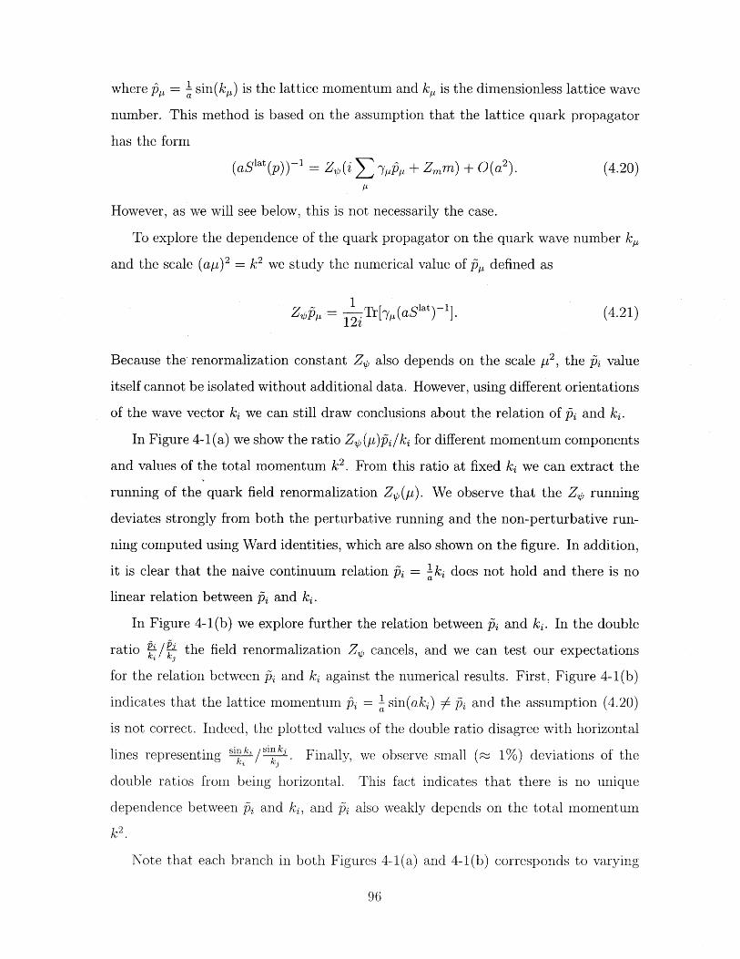
where P, = sin(kg) is the lattice momentum and k, is the dimensionless lattice wave
number. This method is based on the assumption that the lattice quark propagator
has the form
(aSiat (p))-i = Zg (i + ypp, + Zmm) + 0(a 2 ). (4.20)
However, as we will see below, this is not necessarily the case.
To explore the dependence of the quark propagator on the quark wave number kA
and the scale (ap)2 k2 we study the numerical value of &, defined as
Z1 = Tr[-,(aSiat)-1 (4.21)12z'
Because the renormalization constant Z also depends on the scale p 2, the Pi value
itself cannot be isolated without additional data. However, using different orientations
of the wave vector ki we can still draw conclusions about the relation of Pi and ki.
In Figure 4-1 (a) we show the ratio Zp (p)P/kj for different momentum components
and values of the total momentum k2. From this ratio at fixed ki we can extract the
running of the quark field renormalization ZO(p). We observe that the Zp running
deviates strongly from both the perturbative running and the non-perturbative run-
ning computed using Ward identities, which are also shown on the figure. In addition,
it is clear that the naive continuum relation pi = .1ki does not hold and there is no
linear relation between Pi and ki.
In Figure 4-1(b) we explore further the relation between i and ki. In the double
ratio the field renormalization Zp cancels, and we can test our expectations
for the relation between Pi and ki against the numerical results. First, Figure 4-1(b)
indicates that the lattice momentum Pi = i sin(aki) # Pi and the assumption (4.20)
is not correct. Indeed, the plotted values of the double ratio disagree with horizontal
lines representing s /8"7 . Finally, we observe small (~ 1%) deviations of the
double ratios from being horizontal. This fact indicates that there is no unique
dependence between pi and ki, and Pi also weakly depends on the total momentum
k2
Note that each branch in both Figures 4-1(a) and 4-1(b) corresponds to varying
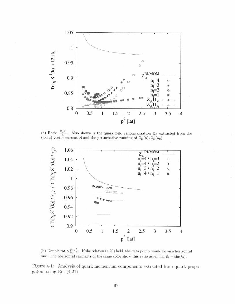
1.05
1
0.95
0.9
0.85
0.8
S RI/MOMni=4ni=3ni=2n.=1 U
* ZA vAZA
0 0.5 1 1.5 2 2.5 3 3.5 4
p2 [lat]
(a) Ratio Z"52. Also shown is the quark field renormalization Zp extracted from the(axial) vector current A and the perturbative running of Zp(p)/Zp(po)
0 0.5 1 1.5 2 2.5 3 3.5 4
p2 [lat]
(b) Double ratio P/2. If the relation (4.20) held, the data points would lie on a horizontalline. The horizontal segments of the same color show this ratio assuming pi = sin(k).
Figure 4-1: Analysis of quark momentum components extracted from quark propa-gators using Eq. (4.21)
C']
H
, G
'RI/MOM 'Zn=4 / n,=3ni=4 / ni=2 .n=3 / n1=2 on1=4 /ni=1
-00+
1.06
1.04
1.02
1
0.98
0.96
0.94
0.92
0.9
HZ
e + o
e WN- an
I I
.. ..... . .
wave number components kj, j # i, thus demonstrating that these branches are
universal and that Pi depends on kj, j # i only through the total momentum k2 .
This dependence cannot be represented through the common factor ZP(k 2 ), and the
general form of a lattice quark propagator is:
(aSlat(p))-l = Z(k2)(i -yap,(ki, k2) + Zm(k 2)m) + O(a2), (4.22)
where the dependence of P,, on k2 is weak but not trivial. Whether this can be
understood as an O(a2) effect is not clear.
Motivated by our findings above, in this work we extract the quark field renor-
malization from vertex functions of operators which satisfy Ward identities and are
not renormalized, instead of Eq. (4.19). In the case of domain wall fermions, we use
the local axial current operator,
A =Op qY5q (4.23)
Because it is only a discretized version of the true partially conserved axial current
A, it is renormalized with a scale-independent factor ZA/ZA =(IAoIQ) and ZA - 1(irjAoIJ2)- 1
(see also Sec. 2.3.3, 4.1.3) also determined from lattice calculations. In the case of
Wilson fermions, there is no conserved axial current, and we have to use the point-
split vector current (4.2) with Zv - 1. In both cases, we extract (eliminate) the
quark field renormalization [B+02, B+04] ZO as
ZV = ZA,VYJA,V, ZO = Z A,v (4.24)'H 0
4.2.4 Vector and axial currents renormalization
Since Domain Wall fermions possess good chiral symmetry, it is instructive to compare
the vertices of local vector and axial vector currents HA and Hv. They are expected to
agree as p 2 -> oc and chiral symmetry breaking effects become less relevant. Figure 4-
2 shows HA,v and their ratio for three quark masses and extrapolation mq -+ 0. The
114
1.13 -0.99
1.12 - - 0.98Zy /OZA
1.11 Cm =0.004111- 0.97 m=0.006
.. .. m =0.0080.96 0
1.09 0.95
1.080.94
1.07_0 2 4 6 8 10 12 141.07 1 2 21 1.5 2 2.5 3 3.5 2 [GeV2
g [GeV]
(a) HA,V for the lightest pion mass m, ~ (b) ZV/ZA - A/fly for three pion masses and300 MeV extrapolation (mq + mres) -> 0
Figure 4-2: Comparison of vector and axial vector renormalization constants in theDomain Wall calculations.
main working region, as we will see below, will be limited to p 2 > 6 GeV 2 or (ap)2 y 1
In Section 4.3.3 we will implicitly use ZA -(11A + Uv) as an estimate of Zp(p), and
from Fig. 4-2 its error is
6ZO 6(UIA -|-Uy) 11A - Uy|~ ~ < 0.25% (4.25)ZI HA + HV IA + HV
because the relative error in ZA is negligible.
Figure 4-3(a) shows ratios of renormalization constants for helicity-dependent and
helicity-independent operators. Because of chiral symmetry, these coefficients must
be equal. All ratios in Fig. 4-3(a) are very close to one indicating that chiral symmetry
breaking effects in the renormalization are negligible. In the following sections, both
helicity-independent and helicity-dependent operators will be renormalized with the
same sets of coefficients.
4.3 Matching to the MS scheme
In order to extract the coefficients which transform the lattice operators to the MS
scheme, we have to
1. Extract the scale-independent (SI) factors between the lattice and RI'-MOM-
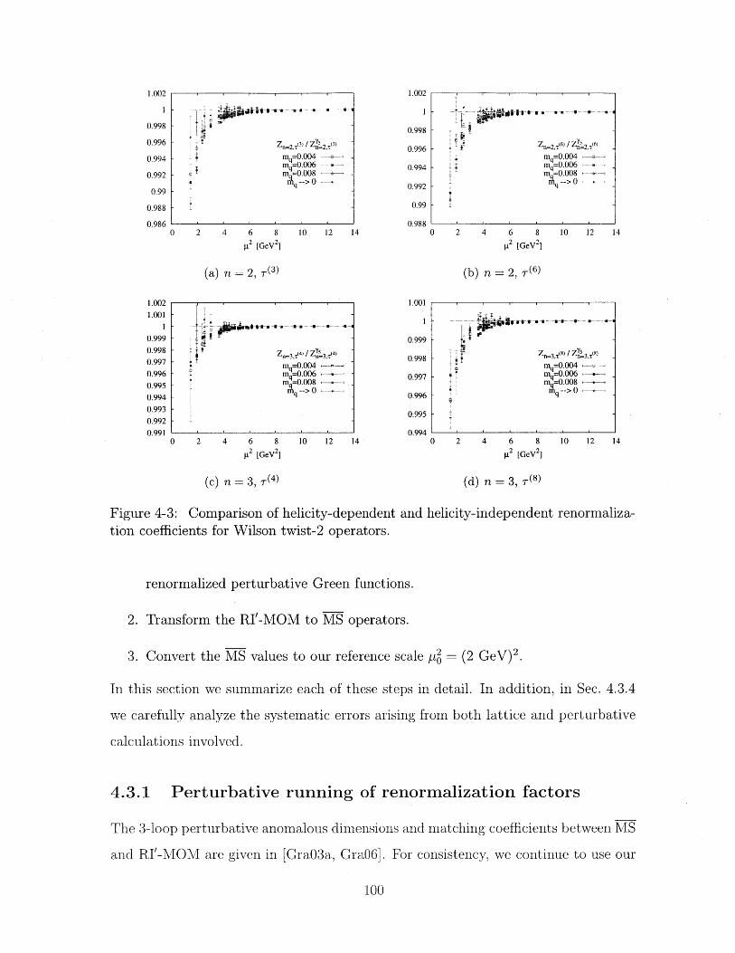
1.002
0.998
0.996
0.994
0.992
0.99
0.9880 2 4 6 8 10 12 14
p2 [GeV2
(a) n = 2, T(3
)
1.001
0.999
0.998
0.997
0.996
0.995
0.994
(4)/Z7 (4)
Zn-3,t Z=34mq=0.0 0 4
- ~ ~ M m=0.006 - -- -mq=0.008
S->0
0 2 4 6 8 10 12 14
s2 [GeV2
(c) n = 3, r(4)
&A
Zn23) Z 2
,(3)
m =0.004mg=0.006
. q m=0 .008q
(d) n = 3, r(8)
Figure 4-3: Comparison of helicity-dependent and helicity-independent renormaliza-tion coefficients for Wilson twist-2 operators.
renormalized perturbative Green functions.
2. Transform the RI'-MOM to MS operators.
3. Convert the MS values to our reference scale yo2 = (2 GeV) 2.
In this section we summarize each of these steps in detail. In addition, in Sec. 4.3.4
we carefully analyze the systematic errors arising from both lattice and perturbative
calculations involved.
4.3.1 Perturbative running of renormalization factors
The 3-loop perturbative anomalous dimensions and matching coefficients between MS
and RI'-MOM are given in [Gra03a, Gra06]. For consistency, we continue to use our
100
1.002
0.998
0.996
0.994
0.992
0.99
0.988
0.986
.... ....
Zn=2,6) / Z 2 6m =0.004mq=O.O
mq=OOO8
m 0008
-q 0
0 2 4 6 8 10 12 14
g2 [GeV2
(b) n 2, r(6)
Zn=3,) / Z1 3 (8)
mq=0.004
mq=0.006
m =0.008- 0
0 2 4 6 8 10 12 14
g2 [GeV2]
1.0021.001
0.9990.9980.9970.9960.9950.9940.9930.9920.991
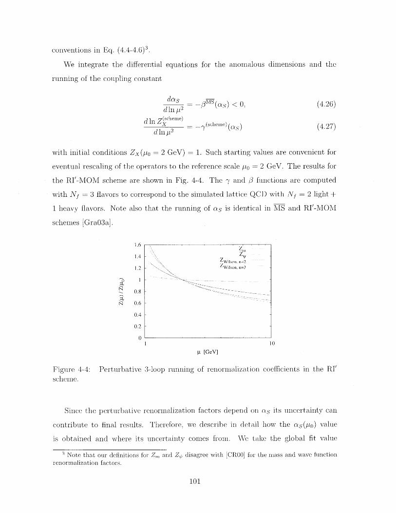
conventions in Eq. (4.4-4.6)3.
We integrate the differential equations for the anomalous dimensions and the
running of the coupling constant
do'das s2 M(as) < 0,d In y
d In Z(chem)scheme)
x 2 (cheme)d hn p_2- -7 (s
(4.26)
(4.27)
with initial conditions Zx(po = 2 GeV) = 1. Such starting values are convenient for
eventual rescaling of the operators to the reference scale pto = 2 GeV. The results for
the RI'-MOM scheme are shown in Fig. 4-4. The -y and # functions are computed
with Nf = 3 flavors to correspond to the simulated lattice QCD with Nf = 2 light +
1 heavy flavors. Note also that the running of as is identical in MS and RI'-MOM
schemes [Gra03a].
pt [GeV]
Figure 4-4: Perturbativescheme.
3-loop running of renormalization coefficients in the RI'
Since the perturbative renormalization factors depend on as its uncertainty can
contribute to final results. Therefore, we describe in detail how the as(po) value
is obtained and where its uncertainty comes from. We take the global fit value
3 Note that our definitions for Zm, and Z, disagree with [CR00] for the mass and wave function
renormalization factors.
101
zn 3Wilson, n=2
ZWfson, n=3-
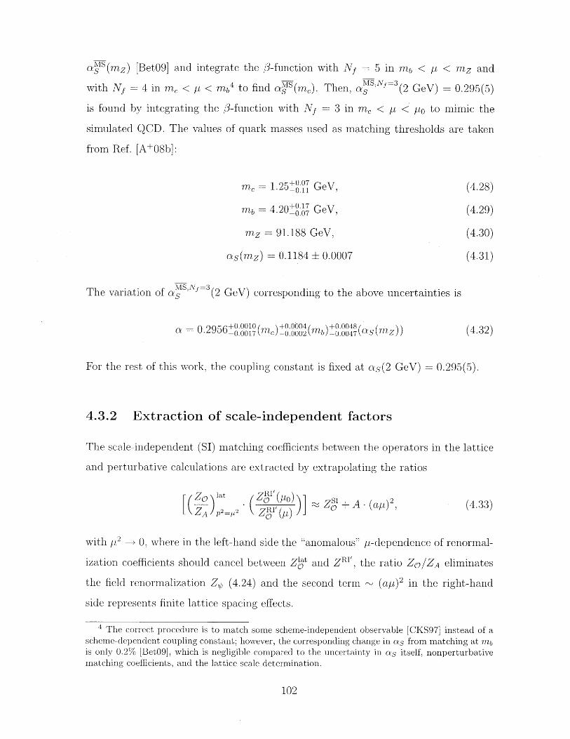
asis(mz) [Bet09] and integrate the /3-function with Nf 5 in mb < p < mz and
with Nf = 4 in mc < p- < mb to find a'(me) Then, aMS,Nf =3(2 GeV) = 0.295(5)
is found by integrating the 7-function with Nf = 3 in m, < p < po to mimic the
simulated QCD. The values of quark masses used as matching thresholds are taken
from Ref. [A+08b]:
mc = 1.25+0 0 GeV,
mb = 4.20+0- GeV,
mz = 91.188 GeV,
(4.28)
(4.29)
(4.30)
(4.31)as(mz) = 0.1184 ± 0.0007
The variation of a MS,Nf:S :3(2 GeV) corresponding to the above uncertainties is
a = 0.2956-.0 -(c0(m7 (a nz)) (4.32)
For the rest of this work, the coupling constant is fixed at as(2 GeV) = 0.295(5).
4.3.2 Extraction of scale- independent factors
The scale-independent (SI) matching coefficients between the operators in the lattice
and perturbative calculations are extracted by extrapolating the ratios
Zo ) latZA p2 12
with [p2 - 0, where in the left-hand side the "anomalous" [[-dependence of renormal-
ization coefficients should cancel between Zat and ZRI', the ratio ZO/ZA eliminates
the field renormalization Zp (4.24) and the second term ~ (ap)2 in the right-hand
side represents finite lattice spacing effects.
4 The correct procedure is to match some scheme-independent observable [CKS97] instead of ascheme-dependent coupling constant; however, the corresponding change in as from matching at mbis only 0.2% [Bet09], which is negligible compared to the uncertainty in as itself, nonperturbativematching coefficients, and the lattice scale determination.
102
(4.33)RI' ~O ZOS + A - (apt) 2,Zo (p)
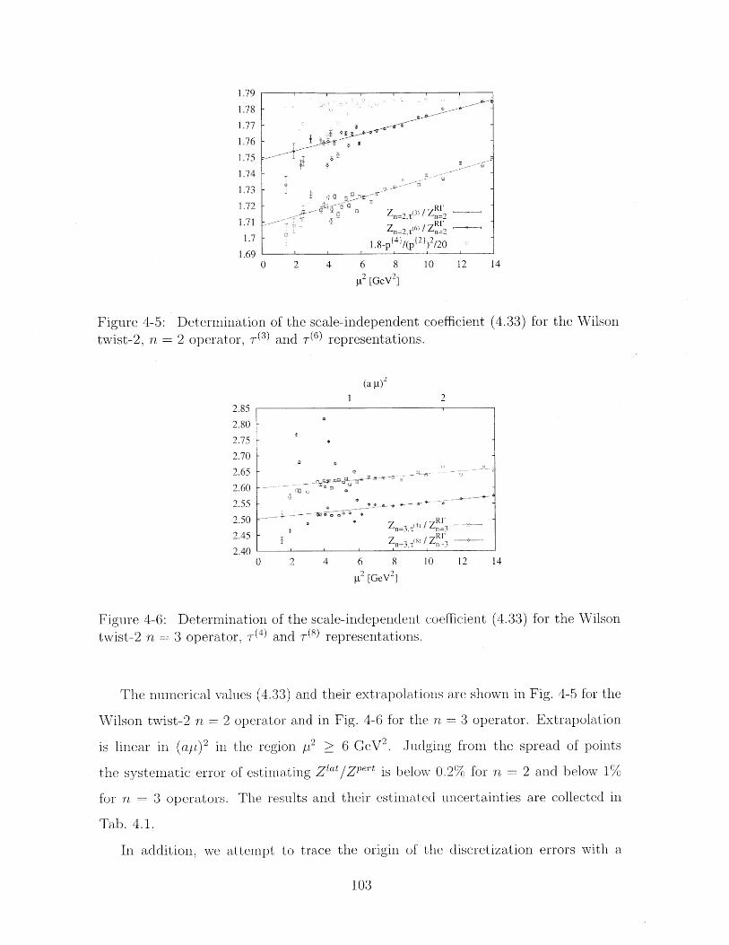
1.79
1.78
1.77
1.76
1.75
1.74
1.73
1.72
1.71
1.7
1.69
Figure 4-5: Determinationtwist-2, n = 2 operator, r(3)
2.85
2.80 -
2.75 -
2.70 -
2.65 -
2.60
2.55
2.50
2.45
2.40
of the scale-independent coefficient (4.33) for the Wilsonand r(6) representations.
(a t)z
0 2 4 6 8 10 12 14
S2 [GeV 2]
Figure 4-6:twist-2 n =
Determination of the scale-independent coefficient (4.33) for the Wilson
3 operator, T() and 7(8) representations.
The numerical values (4.33) and their extrapolations are shown in Fig. 4-5 for the
Wilson twist-2 n = 2 operator and in Fig. 4-6 for the n = 3 operator. Extrapolation
is linear in (at)2 in the region p 2 > 6 GeV 2 . Judging from the spread of points
the systematic error of estimating Zlat/Zpert is below 0.2% for n = 2 and below 1%
for n = 3 operators. The results and their estimated uncertainties are collected inl
Tab. 4.1.
In addition, we attempt to trace the origin of the discretization errors with a
103
z ( 3) Z I
-n-
- Z) 2 / Z
1.8-p 4 /(p 21 220
0 2 4 6 8 10 12 14
.t2 [GeV2
Z 3 (4) RI
Z- 3R1
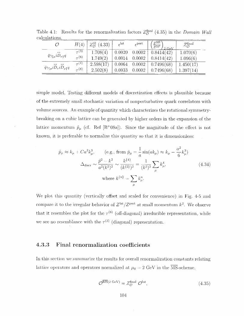
Table 4.1: Results for the renormalization factors Znal (4.35) in the Domain Wallcalculations.
O H (4) Zs' (4.33) at pert Z Zinal7-(3)I
2 GeV
7(3) 1.708(4) 0.0020 0.0002 0.8414(42) 1.070(6)q{,zDL,}q 7(6) 1.749(2) 0.0014 0.0002 0.8414(42) 1.096(6)
r(4) 2.598(17) 0.0064 0.0002 0.7496(68) 1.450(17)q',zDLiDq 7(8) 2.502(8) 0.0033 0.0002 0.7496(68) 1.397(14)
simple model, Testing different models of discretization effects is plausible because
of the extremely small stochastic variation of nonperturbative quark correlators with
volume sources. An example of quantity which characterizes the rotational symmetry-
breaking on a cubic lattice can be generated by higher orders in the expansion of the
lattice momentum , (cf. Ref [B+08a]). Since the magnitude of the effect is not
known, it is preferable to normalize this quantity so that it is dimensionless:
Ca2 k ,2
p2Adiscr 2
(e.g., from p, - I sin(ak,,) k, - k )
- k 2 kN 11
((2)2 {2})2 (k2)2
wh (k " " it
where kO' 1 Zk>r
We plot this quantity (vertically offset and scaled for convenience) in Fig. 4-5 and
compare it to the irregular behavior of Zlat/ZPert at small momentum k2 . We observe
that it resembles the plot for the (6) (off-diagonal) irreducible representation, while
we see no resemblance with the (3) (diagonal) representation.
4.3.3 Final renormalization coefficients
In this section we summarize the results for overall renormalization constants relating
lattice operators and operators normalized at to = 2 GeV in the MS-scheme,
0 Ms(2 Gev) =Zinal 0 iat (4.35)
104
pAt~ kit +
(4.34)
for the quark-bilinear operator studied in Chap. 5. The overall renormalization con-
stant is computed as the combination
Znai =Zia (Zr) Zo lat ZR'(po) )(4.36)OG A 0)Z Zl(p (a/t)2__o'
scale-independent ZS'
where the first factor ZA = 0.74470(6) was determined in Ref. [S+10], the second
factor is a 3-loop conversion function [CRI' (aS(IO))] 1 (ZS/ZRI'), 0 and the third
factor is extracted as described in Sec. 4.3.2. The final results for renormalization
coefficients in the Domain Wall calculations are collected in Tab. 4.1. Column elat
shows fractional error from lattice calculations, and column eper shows fractional
error from perturbative anomalous dimensions. The latter will be discussed in detail
in Sec. 4.3.4. The error from the conversion function CRI'(cs([bo)) is given below
in Tab.4.2. All the uncertainties including 6Zp (4.25) are added in quadrature and
shown in the last column Zinal
4.3.4 Systematic errors
There are several different sources of uncertainty in the determination of non-perturbative
renormalization factors. We study each source separately to find out which has the
most influence. First of all, we note that the stochastic fluctuation of the lattice
correlators is negligible, compared, for example, to the nonlinearity of (Zlat/ZR.I') in
(ap)2 , and it will not be discussed further. The other sources of errors fall into the
following categories:
" irregular (nonlinear) dependence of (Zlat/ZRI') on (at)2 ;
* uncertainty in the strong coupling as;
" perturbative series truncation.
Note that the uncertainty in as and the truncation of perturbative series con-
tribute to Z.nai in two distinct ways. First, the variation in the slope of (Zlat/ZRV)
105
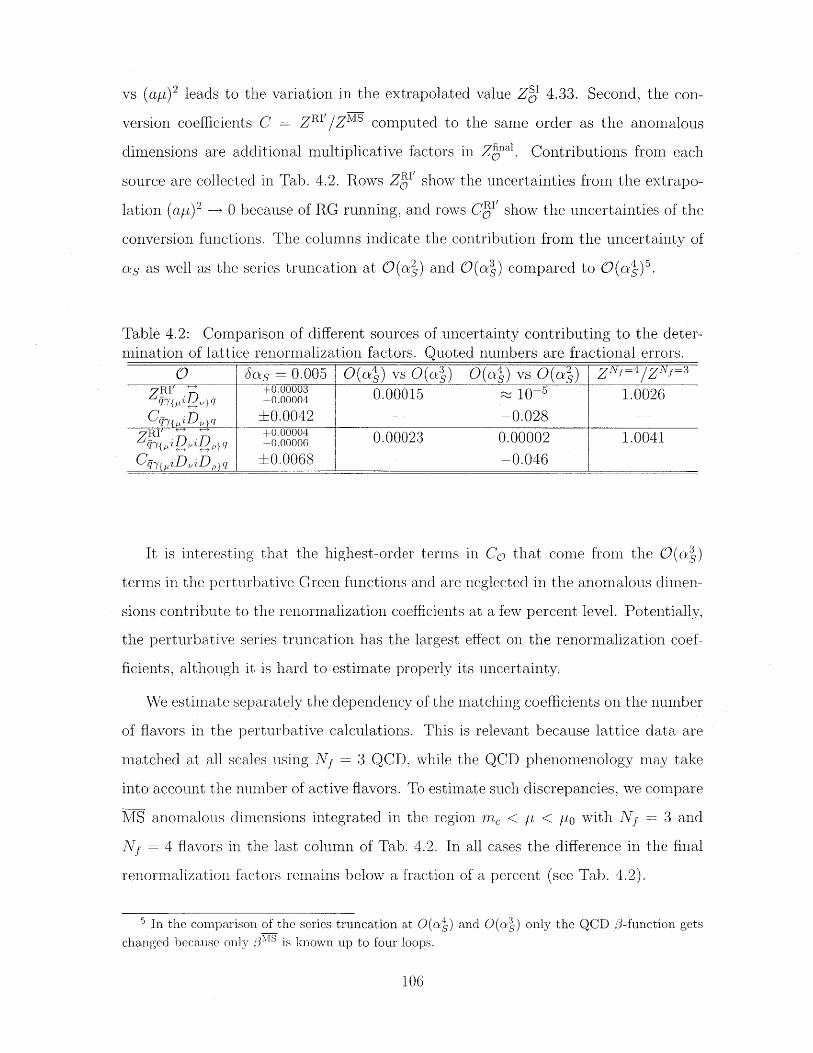
vs (apt) 2 leads to the variation in the extrapolated value Zs' 4.33. Second, the con-
version coefficients C = ZRI'/ZMs computed to the same order as the anomalous
dimensions are additional multiplicative factors in Znal. Contributions from each
source are collected in Tab. 4.2. Rows Z"' show the uncertainties from the extrapo-
lation (ap)2 -> 0 because of RG running, and rows Cs' show the uncertainties of the
conversion functions. The columns indicate the contribution from the uncertainty of
as as well as the series truncation at O(av) and Q(a3) compared to O(a4)'.
Table 4.2: Comparison of different sources of uncertainty contributing to the deter-mination of lattice renormalization factors. Quoted numbers are fractional errors.
O -as = 0.005 O(ac) vs O(as) O(a4) vs O(as) ZNJ=4 /Ng=3
+0.00004 0.00015 10 1.0026
Cqy piDq ±0.0042 -0.028ZtY iD~iDpjq 0.00023 0.00002 1.0041
Cqy{,iDviDP q ±0.0068 -0.046
It is interesting that the highest-order terms in Cc that come from the O(a3)
terms in the perturbative Green functions and are neglected in the anomalous dimen-
sions contribute to the renormalization coefficients at a few percent level. Potentially,
the perturbative series truncation has the largest effect on the renormalization coef-
ficients, although it is hard to estimate properly its uncertainty.
We estimate separately the dependency of the matching coefficients on the number
of flavors in the perturbative calculations. This is relevant because lattice data are
matched at all scales using Nf = 3 QCD, while the QCD phenomenology may take
into account the number of active flavors. To estimate such discrepancies, we compare
IS anomalous dimensions integrated in the region mc < pt < pto with NJ = 3 and
Nf = 4 flavors in the last column of Tab. 4.2. In all cases the difference in the final
renormalization factors remains below a fraction of a percent (see Tab. 4.2).
5 In the comparison of the series truncation at O(a) and O(a.) only the QCD #-function getschanged because only 0"S is known up to four loops.
106
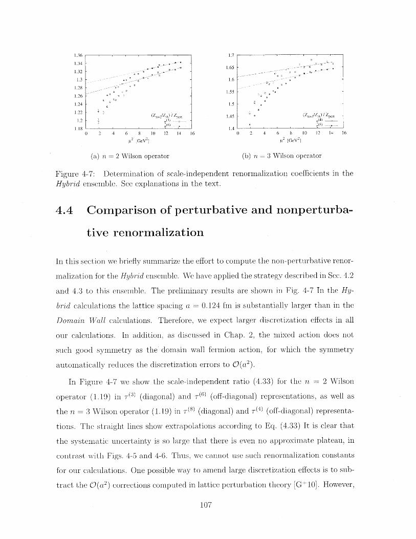
1.36 1.7
1 .3 4 1 .651.6 5
1.32
1.3 - 1.6
1.28 -
1.26 1.55
1.24 1.5
~~ (Z,_2/ZA) ZpeI t 1.45 - (Z _/ZA) /Zprt1.2 T (34
1.18 - 1.4 '
0 2 4 6 8 10 12 14 16 0 2 4 6 8 10 12 14 16
p2 [GeV21 p2 [GeV
2]
(a) n = 2 Wilson operator (b) n = 3 Wilson operator
Figure 4-7: Determination of scale-independent renormalization coefficients in the
Hybrid ensemble. See explanations in the text.
4.4 Comparison of perturbative and nonperturba-
tive renormalization
In this section we briefly summarize the effort to compute the non-perturbative renor-
malization for the Hybrid ensemble. We have applied the strategy described in Sec. 4.2
and 4.3 to this ensemble. The preliminary results are shown in Fig. 4-7 In the Hy-
brid calculations the lattice spacing a = 0.124 fin is substantially larger than in the
Domain Wall calculations. Therefore, we expect larger discretization effects in all
our calculations. In addition, as discussed in Chap. 2, the mixed action does not
such good synmnetry as the domain wall fermion action, for which the symmetry
automatically reduces the discretization errors to 0(a 2).
In Figure 4-7 we show the scale-independent ratio (4.33) for the n = 2 Wilson
operator (1.19) in r(3) (diagonal) and r(6) (off-diagonal) representations, as well as
the n = 3 Wilson operator (1.19) in T(') (diagonal) and r(4) (off-diagonal) representa-
tions. The straight lines show extrapolations according to Eq. (4.33) It is clear that
the systematic uncertainty is so large that there is even no approximate plateau, in
contrast with Figs. 4-5 and 4-6. Thus, we cannot use such renormalization constants
for our calculations. One possible way to amend large discretization effects is to sub-
tract the 0(a 2 ) corrections computed in lattice perturbation theory [G+10]. However,
107
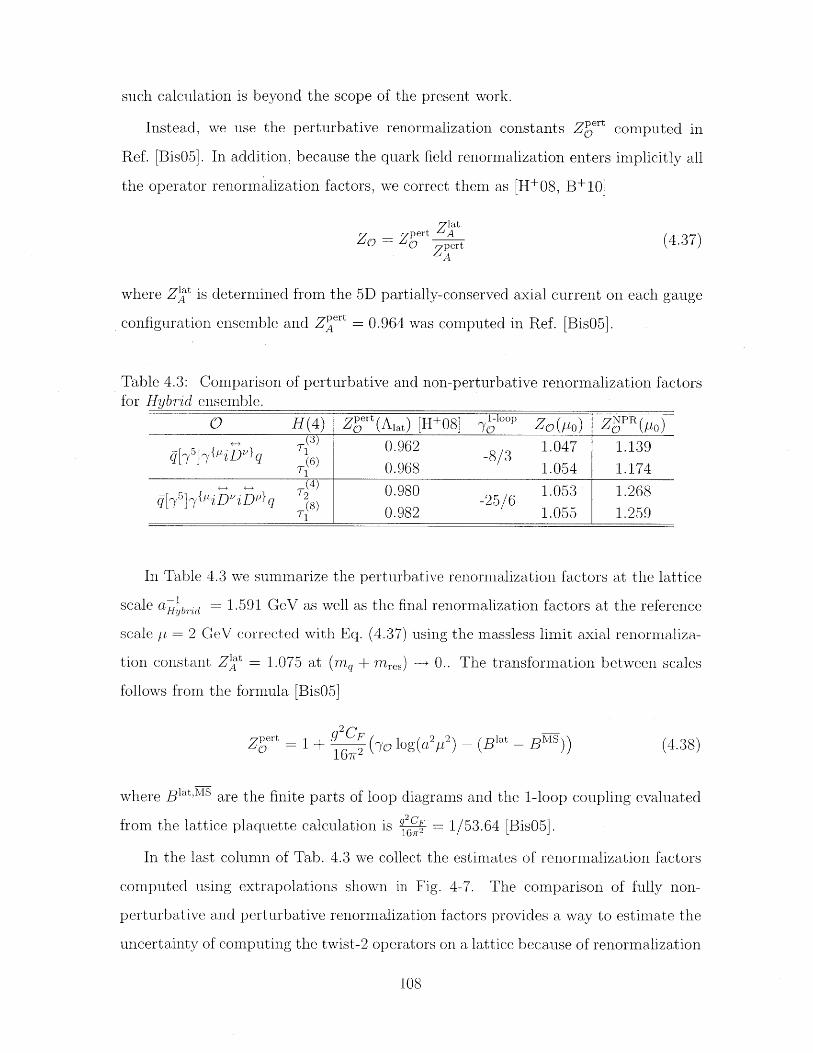
such calculation is beyond the scope of the present work.
Instead, we use the perturbative renormalization constants Zert computed in
Ref. [Bis05]. In addition, because the quark field renormalization enters implicitly all
the operator renormalization factors, we correct them as [H+08, B+10]
ZiatZO = ZPert A (4.37)
where Zlt is determined from the 5D partially-conserved axial current on each gauge
configuration ensemble and Zpert = 0.964 was computed in Ref. [Bis05].
Table 4.3: Comparison of perturbative and non-perturbative renormalization factorsfor Hybrid ensemble.
O H (4) Zpe""(Alt) [H+08] 71-0- Z(po) ZNPR(
[-"(3) 0.962 1.047 1.139q[ (6) 0.968q T -8/3
i0.968 1.054 1.174
T2"4r 0.980 1.053 1.268r( 0.982 1.055 1.259
In Table 4.3 we summarize the perturbative renormalization factors at the lattice
scale a =b = 1.591 GeV as well as the final renormalization factors at the reference
scale y = 2 GeV corrected with Eq. (4.37) using the massless limit axial renormaliza-
tion constant Z>' = 1.075 at (mq + mres) -+ 0.. The transformation between scales
follows from the formula [BisO5]
Zpert = + .162 F ('O log (a2[t
2 ) (Blat -Bus)) (4.38)
where Biat'S are the finite parts of loop diagrams and the I-loop coupling evaluated
from the lattice plaquette calculation is 92c = 1/53.64 [Bis05].
In the last column of Tab. 4.3 we collect the estimates of renormalization factors
computed using extrapolations shown in Fig. 4-7. The comparison of fully non-
perturbative and perturbative renormalization factors provides a way to estimate the
uncertainty of computing the twist-2 operators on a lattice because of renormalization
108
in Hybrid calculations:
n = 2 Zo/Z ~ 6%,
n - 3 6Zo/Zo 10%.
Summary
In this section, we have calculated the renormalization constants for the twist-two
lattice operators of rank n = 2 and n = 3 nonperturbatively for the Domain Wall
lattices. We use the standard procedure described in the literature on lattice opera-
tor renormalization, which provides precise determination of lattice renormalization
factors even with small statistics.
We repeated a similar calculation for the Hybrid lattices, for which perturbative
calculation of renormalization constants previously existed, to compare the lattice and
analytic determinations. Nonperturbative renormalization is problematic because the
scale window AQCD < p < a I nay not exist or very narrow. Nevertheless, the
results of the perturbative and lattice calculations agree within ~ 10% and allow us
to estimate the systematic error because of the renormalization of lattice operators
in the Hybrid calculations.
109

110
Chapter 5
Select Results
Equipped with the methods summarized in the previous chapters, we can compute a
wide array of nucleon structure observables. To demonstrate how these calculations
compare to experiments, in this section we present our results, including vector form
factors and charge/magnetization radii in Sec. 5.1 for isovector and 5.2 for isoscalar
components, axial charge and form factors in Sec. 5.3, quark contributions to nucleon
momentum and spin in Sec. 5.4, and generalized form factors in Sec. 5.5. In addition,
we can assess the systematic uncertainties of our calculations by comparing the results
obtained using different lattice QCD discretizations listed in Appendix A.
Since our calculations are done with pion masses m, > 300 MeV we use chiral ex-
trapolations to obtain physical observables at the physical pion mass m - 140 MeV.
Generally, there is little understanding of whether a particular formulation of baryon
ChPT is adequate for the range of pion masses we are working with. In addition,
the applicability of different formulations of baryon ChPT may depend on nucleon
structure observables in question. Throughout this section we will use the following
baryon ChPT formulations:
" CBChPT , [covariant] baryon chiral perturbation theory, in which baryons and
mesons are relativistic [GSSS8];
" HBChPT , heavy baryon chiral perturbation theory, additional expansion in
m,-/MN with consistent power counting demonstrated in Ref. [BKKM92];
111
* HBChPT+A , heavy baryon chiral perturbation theory including the A(1232)
degree of freedom, also called Small Scale Expansion (SSE) [HHK98].
For completeness, we summarize the details of these formulations in Appendix D.
Although we perform full QCD simulations with dynamical Nf = 2 + 1 flavors, in
all our ensembles the s-quark has a fixed mass near its physical value. Therefore, we
have no means to study how the chiral dynamics changes with the s-quark mass and
constrain the ChPT parameters related to the SU(3)f symmetry breaking. For this
reason, we resort to SU(2)f chiral perturbation theory to analyze our data.
5.1 I =1 vector form factors
In this section we present our results for the isovector Dirac and Pauli form factors and
the corresponding r.m.s. radii. After discussing the momentum transfer dependence
of the form factors, we compare the chiral extrapolations for the nucleon radii using
the SSE (HBChPT+A ) and covariant baryon chiral perturbation theory (CBChPT
5.1.1 Momentum transfer dependence
As will be discussed in the following section, ChPT describes the Q2 -dependence
of the form factors for values of Q2 much less than the chiral symmetry breaking
scale (typically of the order of the nucleon mass). Lacking a model-independent
functional form applicable in the large-Q2 region, we study the Q2 dependence using
the phenomenological dipole and tripole formulas. Although there is no theoretical
understanding of this fact, the dipole formula (5.1,5.3) is used to fit experimental
results for the form factors. We also use fits to the tripole formula to show that
the dependence of the extracted radii and the anomalous magnetic moment on the
functional form is irrelevant at our level of precision.
The Dirac form factor is fixed to 1 at Q2 = 0 under our renormalization scheme,
and we use the following one-parameter dipole or tripole formula to describe the Q2
112
dependence:
F((Q) Q2)
1 + _ 2
1
(1 + AT)3
(one-parameter dipole),
(one-parameter tripole).
The Pauli form factor at Q2 = 0, F2(0), cannot be measured on the lattice directly.
We thus fit the data using the two-parameter dipole or tripole formula,
F( F2 (0)( 1+ D 2 )
F2 (Q2) =F2(0)
(1 + A02)
(two-parameter dipole),
(two-parameter tripole).
We are interested in mean squared Dirac and Pauli radii, which are defined by the
slope of the form factors at small Q2:
F1,2(0) 1 -
and are related to the pole masses by
for the dipole fits, and
(r
for the tripole fits.
- (ri,2) 2 Q2 +6
AD 2 ,
Note that results at different Q2 from the same ensemble may be highly corre-
lated [B+08b], therefore we perform correlated least-X2 fits to the data. We investigate
the extent to which the dipole and tripole Ansaitze describe our data and the stability
of the fits by varying the maximum Q2 values included in the fits.
In Table 5.1 we show the fit results for Flj d(Q2) using the one-parameter dipole
and tripole formulas in Eqs. (5.1) and (5.2) for the fine Domain Wall lattice with
113
F1(Q2) =
(5.1)
(5.2)
(5.3)
(5.4)
C(Q4)]
(5.6)
(5.7)
F1, 2(Q2) =
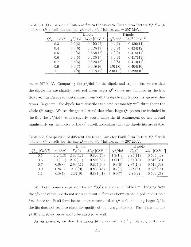
Table 5.1: Comparison of different fits to the isovector Dirac form factors Ff-d withdifferent Q2 cutoffs for the fine Domain Wall lattice, m, = 297 MeV.
Dipole Tripole
QMax [GeV2 2 /dof M3 [GeV 2 /dof M- 2 [GeV -2]0.3 0.2(6) 0.670(22) 0.2(6) 0.436(14)0.4 0.3(6) 0.659(19) 0.8(9) 0.424(12)0.5 0.5(6) 0.653(17) 1.0(9) 0.418(11)0.6 0.4(5) 0.652(17) 1.0(8) 0.417(11)0.7 0.5(5) 0.649(17) 1.2(8) 0.414(11)0.9 0.9(7) 0.638(16) 1.9(1.0) 0.404(10)1.1 1.4(8) 0.632(16) 3.0(1.1) 0.398(10)
m, = 297 MeV. Comparing the X2 /dof for the dipole and tripole fits, we see that
the dipole fits are slightly preferred when larger Q2 values are included in the fits.
However, the Dirac radii determined from both the dipole and tripole fits agree within
errors. In general, the dipole form describes the data reasonably well throughout the
whole Q2 range. We see the general trend that when large Q2 points are included in
the fits, the / 2/dof becomes slightly worse, while the fit parameters do not depend
significantly on the choice of the Q2 cutoff, indicating that the dipole fits are stable.
Table 5.2: Comparisondifferent Q2 cutoffs for
of different fits to the isovector Pauli form factors F L-d withthe fine Domain Wall lattice, m , = 297 MeV.
Dipole Tripole
Qnax [GeV2 2 /dof F2 (0) MD2 [GeV -2] 2 /dof F2 (0) M 2 [GeV-2]0.5 1.2(1.3) 2.89(12) 0.820(70) 1.2(1.3) 2.85(11) 0.505(40)0.6 1.1(1.1) 2.92(11) 0.846(63) 1.0(1.0) 2.87(10) 0.516(36)0.7 0.9(8) 2.93(11) 0.847(60) 0.8(8) 2.87(10) 0.513(33)0.9 0.9(8) 2.98(9) 0.888(46) 0.7(7) 2.89(8) 0.526(15)1.1 0.8(7) 2.97(9) 0.881(41) 0.9(7) 2.85(8) 0.509(21)
We do the same comparison for F2d(Q2) as shown in Table 5.2. Judging from
the X2/dof values, we do not see significant differences between the dipole and tripole
fits. Since the Pauli form factor is not constrained at Q2 = 0, including larger Q2 in
the fits does not seem to affect the quality of the fits significantly. The fit parameters
F2 (0) and MD,T prove rot to be affected as well.
As an example, we show the dipole fit curves with a Q2 cutoff at 0.5, 0.7 and
114
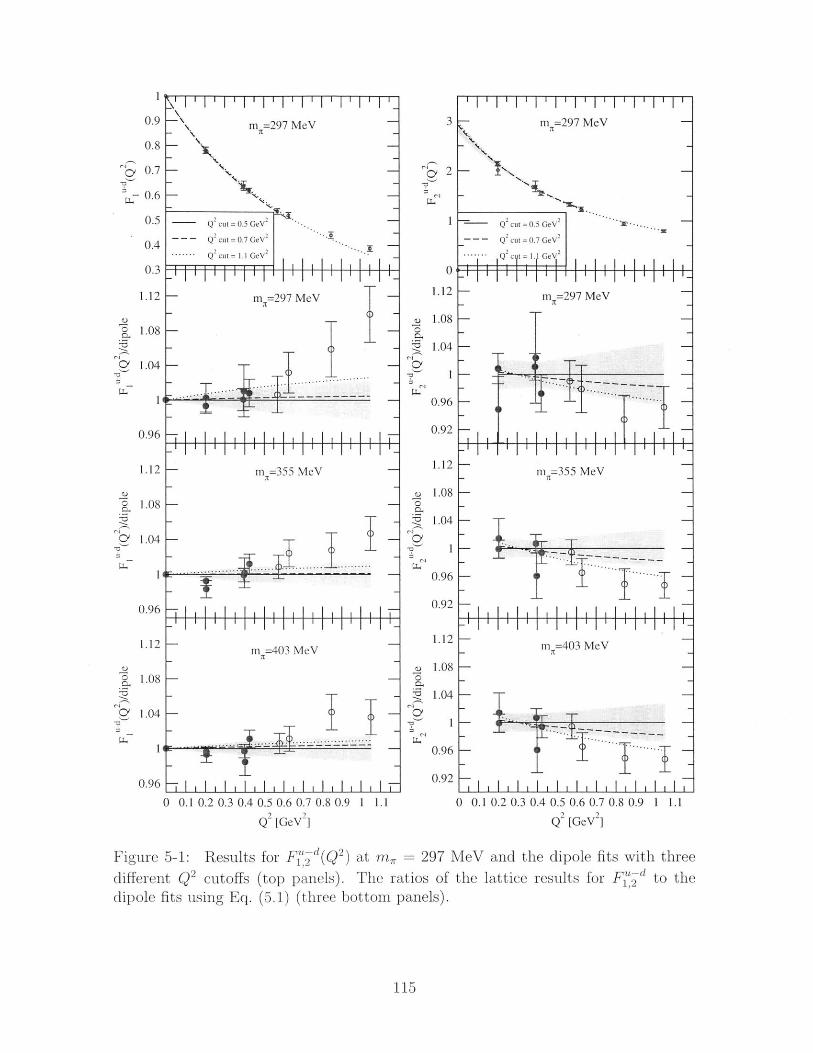
Figure 5-1:
0.9 -m =297 MeV
0.8
0.7
0.6
0.5 - Q2 Cut = .5 GeV -
0.4 Qcut=0.7GeV
0.3
1.1211.12 -m =297 MeV
1.12 m =3 MeV
1.08 -- -
1[04 --
0.96 _
1.12 - m =43 MeV _
1.08 -
1.04 --
0--6
1.12 - m 40G eV .
-3
04
3
2
0
1.12
1.08
1.04
0.96
0.92
1.12
1.08
1.04
1
0.96
0.92
1.12
1.08
1.04
1
0.96
0.92
0 0.1 0.2 0.3 0.4 0.5 0.6 0.7 0.8 0.9 1 1.1
Q [GeV2
Results for F,2d(Q2) at m, = 297 MeV and the dipole fits with threedifferent Q2 cutoffs (top panels). The ratios of the lattice results for Fd to thedipole fits using Eq. (5.1) (three bottom panels).
115
-3
0
1.1 GeV 2 for the m, = 297 MeV ensemble in the top panel of Fig. 5-1. To show
the quality of the fits more clearly, we plot the ratios of the form factor data to the
dipole fit with the Q2 cutoff at 0.5 GeV2 in the bottom three panels of Fig. 5-1.
The error bands reflect the jackknife errors in the dipole fit parameters. We see that
although the data included in the fits can be described reasonably well by the dipole
formula with discrepancies that are generally within 2 to 3 standard deviations, the
clear systematic tendency indicates that the dipole Ansatz is not a good description
of the data over the whole momentum transfer region. In particular, for Fl-d, the
precisely measured points in the region of 0.2 GeV2 are systematically lower than
the dipole fit, whereas at high Q2, the lattice data are systematically higher. For
Fuj , the high Q2 lattice data are systematically lower than the dipole fit. This is
consistent with the empirical fits to the experimental data in Refs. [FW03, AMT07],
where the phenomenological corrections to the dipole form are negative in the region
of 0.2 GeV 2 and positive at about 0.4 GeV 2. For comparison, we also plot the dipole
fits with Q2 cutoffs at 0.7 GeV 2 (dashed line) and 1.1 GeV2 (dotted line) relative to
the 0.5 GeV 2 dipole fit (solid line). The differences between different Q2 cutoffs are
small, indicating that the fits are stable.
It is worth noting that the Dirac and Pauli radii, rj and r', and the anomalous
magnetic moment, rv, are defined in the Q2 = 0 limit. We thus restrict the fits
to the smallest Q2 points possible to extract these quantities while still including
enough data points to constrain the fits. For uniformity we choose to determine these
quantities from the one-parameter dipole fits for F,-- , and the two-parameter dipole
fits for F--d, with a Q2 cutoff at 0.5 GeV2.
We also perform dipole fits to GE(Q 2) and GAI(Q 2) to see how well the dipole
Ansatz describes the data. We find that the dipole fits to G'-d and G'-d are qual-
itatively similar to Ff--d and F2jd. However, it appears that the fits are even more
stable over the whole range of Q2 than Dirac and Pauli form factors. This is indicated
by little change in the ratio plots in Fig. 5-2 with different Q2 cutoffs.
Figure 5-3 shows a comparison of the lattice results for GE at three different pion
masses from the fine ensembles (the lattice spacing a = 0.084 fm) and one pion mass
116
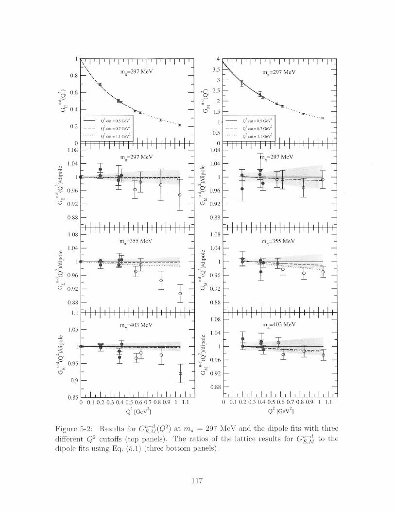
4
0.8 n=297 MeV 3.5 m =297 MeV
0.83-
06 2.5
0.4 1.5
02Q 2cut = 0.5 GeV --.. Q 2cut = 0.5 GeV2Q. cut = 0.7 GeV - -- Q cut = 0.7 GeV-
-... Q Cut = 1. 1 GeV 0 . ... cut = 1.1 GeV
0 01.08 1.08
-m =297 MeV - =297 MeV1.04 -1.04
0.96 -0.96
0.92 0.92
0.88 - 0.88
108 -- 1.08m =355 MeV m =355 MeV
1.04 - 1.04
1 -- -
0.96 --- 0.96
0.92 0 0.92
0.88 0.88
1.08
1.05 rn=403 MeV m =403 MeV1.04
-~Q~ 0.960.95 --- - -
0 0 0.920.9
0.850.880 0.1 0.2 0.3 0.4 0.5 0.6 0.7 0.8 0.9 1 1.1 0 0.1 0.2 0.3 0.4 0.5 0.6 0.7 0.8 0.9 1 1.1
Q [GeV 2 Q [GeV ]
Figure 5-2: Results for G - (Q2) at m, 297 MeV and the dipole fits with threedifferent Q2 cutoffs (top panels). The ratios of the lattice results for G'- d to thedipole fits using Eq. (5.1) (three bottom panels).
117
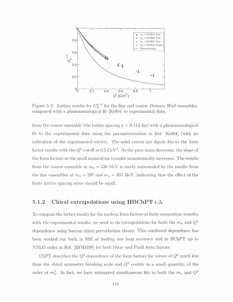
0.6-
0.4-
0.2 --
0 0.2 0.4 0.6 0.8 1
Q2 [GeV2
Figure 5-3: Lattice results for G -d for the fine and coarse Domain Wall ensembles,compared with a phenomenological fit [Ke104] to experimental data.
from the coarse ensemble (the lattice spacing a = 0.114 fin) with a phenomenological
fit to the experimental data using the parameterization in Ref. [Kel04] (with no
indication of the experimental errors). The solid curves are dipole fits to the form
factor results with the Q2 cutoff at 0.5 GeV2 . As the pion mass decreases, the slope of
the form factors at the small momentum transfer mnonotonically increases. The results
from the coarse ensemble at m, = 330 MeV is nicely surrounded by the results from
the fine ensembles at in, = 297 and m, = 355 MeV, indicating that the effect of the
finite lattice spacing error should be small.
5.1.2 Chiral extrapolations using HBChPT+A
To compare the lattice results for the nucleon form factors at finite momentum transfer
with the experimental results, we need to do extrapolations for both the m, and Q2
dependence using baryon chiral perturbation theory. This combined dependence has
been worked out both in SSE at leading one loop accuracy and in BChPT up to
NNLO order in Ref. [BFHM98] for both Dirac and Pauli form factors.
ChPT describes the Q2 dependence of the form factors for values of Q2 much less
than the chiral symmetry breaking scale and Q2 counts as a small quantity, of the
order of m2. In fact, we have attempted simultaneous fits to both the m., and Q2
118
dependences of Ff -d using the SSE formula in Ref. [BFHM98], and found that the
fits fail to describe data even with Q2 < 0.4 GeV 2 (X 2 /dof ~ 10). This is consistent
with the findings of Ref. [BFHM98], where the applicability of the O(cs) SSE results
for the isovector nucleon form factors at physical pion mass was found to be limited
to Q2 < 0.2 GeV 2 . Lacking a model-independent functional form applicable in the
large-Q 2 region, we resort to studying the pion-mass dependence of the mean squared
Dirac radius, (r') 2, Pauli radius, (r-,) 2 , and the anomalous magnetic moment, Ko,
as obtained from the dipole fits discussed in Sec. 5.1.1. We tabulate these values in
Table 5.3.
Table 5.3: Results for the isovector Dirac and Pauli radii and anomalous magneticmoment from dipole fits with Q2 < 0.5 GeV 2.
m, [MeV] (ru) 2 [fm 2 ] (rv) 2 [fm 2] ,norm (r) 2 [fm 2] norm297 0.305(8) 0.382(33) 0.938(117) 2.447(99)
355 0.281(5) 0.372(18) 0.938(66) 2.518(57)403 0.272(5) 0.379(16) 0.954(58) 2.508(51)330 0.290(9) 0.445(26) 1.230(105) 2.758(84)
Our results for the form factor F 2 and sv are given in terms of a nucleon (hence,
quark) mass-dependent "nmagneton" (see Eq. (1.1)), which is not accounted forN
in SSE at the order at which we are working (see Eq. (D.2) in the Appendix). There-
fore, in order to fit our lattice data to the SSE predictions, we follow Refs.[G+05b,
AKNT06] and define 0n"" measured relative to the physical magneton . A,' :
N. NM/phys M/phys
snorrnm N lat __ Na F2(0). (5.8)
We then identify MN in the SSE expressions as the physical nucleon mass. In the
following comparisons of our results with chiral perturbation theories, the normalized
magnetic moment norm will be used throughout, and we drop the superscript "norm"
unless there is an ambiguity.
As specified in Appendix D.1.1, at the order 0( 3 ) all the couplings in Eqs. (D.2
D.4) are meant to be taken in the chiral limit. Replacing them with the corresponding
quantities at the physical point amounts to the inclusion of higher-order effects. As
119
long as the deviation between the values in the chiral limit and at the physical point
is small, one expects such a replacement to yield little effect. To test this statement,
in some cases we have performed the chiral fits using both the physical values and the
chiral limit values for the low-energy constants and found no significant differences.
In the following we will only present results obtained using the chiral limit values as
inputs, which are summarized in Table 5.4.
Table 5.4: Input values for the low-energy constants in the fits: the nucleon axialcharge YA, the pion decay constant F, and the mass difference A = MA - MN. Thesevalues correspond to the chiral limit m, -+ 0.
9A F, [GeV] A [GeV]1.2 0.0862 0.293
Among the low-energy constants discussed in Appendix D.1.1, CA and cv are the
two least known. In addition, we have little knowledge of the counterterms, B] 0 (A)
and E[(A), as well as the anomalous magnetic moment in the chiral limit, <0, from
phenomenology. Lattice calculations in the chiral regime have the potential to con-
strain these parameters to unprecedented accuracy. Our attempt here is to check
the consistency of our data with the predictions of chiral effective field theories, to
estimate the range of applicability of the ChPT formulas, and to determine these
low-energy constants when the formulas are applicable. To disentangle the inves-
tigation of the applicability of the ChPT formula from the possible discretization
effects, we only include the results from the three fine ensembles in the chiral extrap-
olations discussed below. However, we want to point out that including the coarse
results in the extrapolations does not change the central values of the fit parameters
significantly, nor does it reduce the errors on the parameters since it only adds an
additional interpolating point and does not provide a much stronger constraint on
the parameters.
Since CA appears in the formulas (D.2,D.3,D.4) for (rv')2 , (r5)2 and s,, a simulta-
neous fit to all these three quantities would give a better constraint for the value of
CA. However, we have only three data points for each of these quantities, and 1% alone
has four parameters, three of which [cV, E[(A) and K,] are not constrained by any
120
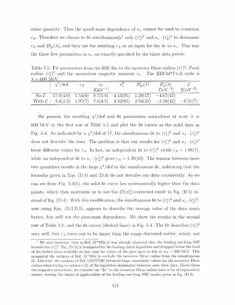
other quantity. Thus the quark-mass dependence of K, cannot be used to constrain
CA. Therefore we choose to fit simultaneously' only (rj)2 and Kv - (rv) 2 to determine
CA and Bljo(A), and then use the resulting CA as an input for the fit to KV. This way
the three free parameters in K. are exactly specified by the three data points.
Table 5.5: Fit parameters from the SSE fits to the isovector Dirac radius (,")2, Pauliradius (r) 2 and the anomalous magnetic moment Ko. The HBChPT+A scale isA = 600 MeV.
2/dof CA cv K 0 B 0 (A) Er[(A) C
[GeV--'] [GeV -3] [GeV -3]No C 17.0(4.0) 1.54(6) 8.7(5.8) 4.13(95) 1.20(17) -4.67(42)
With C 3.8(2.2) 1.97(7) 7.5(4.5) 4.32(95) 2.58(25) -5.58(42) -0.51(7)
We present the resulting y 2 /dof and fit parameters normalized at scale A -
600 MeV in the first row of Table 5.5 and plot the fit curves as the solid lines in
Fig. 5-4. As indicated by a / 2 /dof of 17, the simultaneous fit to (rv) 2 and K., (rK) 2
does not describe the data. The problem is that our results for (r) 2 and i- (rv) 2
favor different values for CA. In fact, an independent fit to (rv) 2 yields CA = 1.98(7),
while an independent fit to 1- (rK) 2 gives CA = 1.39(10). The tension between these
two quantities results in the large X2 /dof in the simultaneous fit, indicating that the
formulas given in Eqs. (D.3) and (D.4) do not describe our data consistently. As we
can see from Fig. 5-4(b), the solid fit curve lies systematically higher than the data
points, which then motivates us to use the ((m0,)-corrected result in Eq. (D.5) in-
stead of Eq. (D.4). With this modification, the simultaneous fit to (r") 2 and V, -(r) 2
now using Eqs. (D.3,D.5), appears to describe the average value of the data much
better, but still not the pion-mass dependence. We show the results in the second
row of Table 5.5, and the fit curves (dashed lines) in Fig. 5-4. The fit describes (r) 2
very well, but cA turns out to be larger than the range discussed earlier, which, not
1 We note however, that in Ref. [G+05b] it was already observed that the leading one-loop SSEformula for (rV)2 [Eq. (D.3)] is dominated by the leading chiral logarithm and dropped below the level
of the lattice data available at that time for values of the pion mass as low as n, < 200 MeV. Thisprompted the authors of Ref. [G+05b] to exclude the isovector Dirac radius from the simultaneousfit. Likewise, the authors of Ref. [AKNT06] obtained huge, unrealistic values for the isovector Diracradius when trying to enforce a fit of the logarithm-dominated behavior onto their data. Given thesetwo negative precedents, we consider our "fit" to the isovector Dirac radius data to be of exploratorynature, testing the limits of applicability of the leading one-loop SSE results given in Eq. (D.3).
121
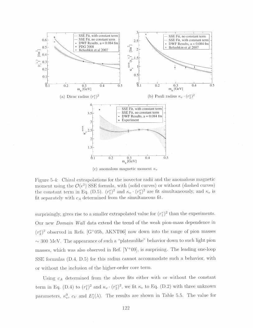
3 I I I I
-- SSE Fit, with constant term - SSE Fit, no constant term0.6 - SSE Fit, no constant term - 2.5 - SSE Fit, with constant term
DWF Results, a = 0.084 fm 5 DWF Results, a = 0.084 fm 0.5B l sna2 2x Belushkin et al 2007_
-XBelushkin et al 2007 2
0.3- 0.3 1.5 -
0.2-
0.1- 0.5-
0.2 0.3 0.4 0.5 l 0.2 0.3 0.4 0.5m [GeV] m, [GeV]
(a) Dirac radius (r,) 2 (b) Pauli radius K, (r2)2
4- --- SSE Fit, with constant term
3.5- - SSE Fit, no constant term- DWF Results, a = 0.084 fm
3 * Experiment
2.5-
2 -
1.5 -
0.2 0.3 0.4 0.5m, [GeV]
(c) anomalous magnetic moment K,
Figure 5-4: Chiral extrapolations for the isovector radii and the anomalous magnetic
moment using the 0(d) SSE formula, with (solid curves) or without (dashed curves)
the constant term in Eq. (D.5). (rv)2 and , (r2) 2 are fit simultaneously, and K, is
fit separately with CA determined from the simultaneous fit.
surprisingly, gives rise to a smaller extrapolated value for (r )2 than the experiments.
Our new Domain Wall data extend the trend of the weak pion-mass dependence in
(rv)2 observed in Refs. [G+05b, AKNT06] now down into the range of pion masses
~ 300 MeV. The appearance of such a "plateaulike" behavior down to such light pion
masses, which was also observed in Ref. [Y+09], is surprising. The leading one-loop
SSE formulas (D.4, D.5) for this radius cannot accommodate such a behavior, with
or without the inclusion of the higher-order core term.
Using CA determined from the above fits either with or without the constant
term in Eq. (D.4) to (rv) 2 and Kv . (r-)2, we fit 'v to Eq. (D.2) with three unknown
parameters, ,, cV and E[(A). The results are shown in Table 5.5. The value for
122
cv from our fit turns out to have a different sign from that determined in [DMW91,
HHK97] mentioned earlier. This is not surprising given that we only have three data
points, which have little or no pion-mass dependence. We do not have the freedom to
check the consistency of the fit, and we do not expect to obtain a reliable estimation
for cv, which, judging from Eq. (D.2), is very sensitive to the curvature of the data.
To compare chiral extrapolations with experiment, we have also plotted selected
experimental data in Fig. 5-4. As noted in the introduction, there are still unresolved
experimental questions, and we have indicated the range of possible values of (r v)2
that can be extracted from present experiments by showing two extreme results from
the literature. The highest value is from PDG 2008 [A+08b] and the lowest value is
from a dispersion analysis including meson continuum contributions [BHM07]. We
note that none of the chiral fits simultaneously yields a good fit to the lattice data
while also agreeing with experiment within statistical errors.
To see how strongly the lattice results deviate from the SSE formulas, we also
try to determine some of the low-energy constants using experimental results at the
physical pion mass. We use the values in Table 5.4 as input, and also set CA =1.5 and
cv = -2.5 GeV-'. Now for (r-v)2, we have only the counter-term B"O to determine.
Constraining the curve to go through the higher experimental value of (r,) 2 = 0.637
fin 2 gives B'0 (A = 600 MeV) = 1.085, resulting in the solid curve shown in Fig. 5-
5(a). For comparison, we also plot the dashed curve that is fixed to go through the
lower experimental value (rv ) 2. The curve rises much more rapidly than the lattice
data as the pion mass decreases. From the slope of the leading one-loop SSE curve
near the physical point and the weak pion-mass dependence displayed by our data we
estimate that the applicability of Eq. (D.3) for (r) 2 may be much less than 300 MeV.
Without the constant term in Eq. (D.5), r% . (r) 2 does not have any free param-
eters, which yields the solid curve in Fig. 5-5(b). The curve undershoots the physical
point by about 5%, which may be well accounted for by the uncertainties in the cho-
sen values of the low-energy constants. Including the higher-order term C of Eq. (D.5)
can of course shift the curve up to exactly reproduce the product of physical Pauli
radius and anomalous magnetic moment. However, the departure of the quark-mass
123
DF R t a = 04 f - - DF R a =DWF Results, a = 0.084 fm DWF Results, a = 0.084 fm
0.6- DWF Results, a =0. 114 fm 2.5- DWF Results, a =0. 114 fmMixed-Action Results, a = 0. 124 fm -. Mixed-Action Results, a 0.124 fm
0.5 - \ * PDG 2008 x Belushkin et al 2007x Belushkin et al 2007 2 -
0.4-1.5-
-0.3 --
0.2 -
0.1 - .. .
1 0.2 0.3 0.4 0.5 0.6 9.1 0.2 0.3 0.4 0.5 0.6m [GeV] m [GeV]
(a) Dirac radius (r") 2 (b) Pauli radius r,. (r )
4DWF Results, a = 0.084 fm
3.5 - DWF Results, a = 0.114 fmMixed-Action Results, a 0.124 fm
3 - * Experiment
~> 2.5
2-
1.5-
0.2 0.3 0.4 0.5 0.6m [GeV]
(c) anomalous magnetic moment K,
Figure 5-5: SSE chiral fits to the isovector radii and the anomalous magnetic momentconstrained to go through the physical points using the input in Table 5.4 as well as
CA = 1.5 and cv = -2.5 GeV-'. The mixed-action results at m, = 355 MeV are
shifted slightly to the right for clarity.
dependent curve from the lattice data displayed in Fig. 5-5(b) indicates that the lead-
ing one-loop SSE formula for r- (rv) 2 of Eqs. (D.4, D.5) should only be trusted for
pion masses much less than the currently available 300 MeV. Judging from the steep
slopes displayed by both the curves for the Dirac and Pauli radii as opposed to the
almost mass-independent nature of the lattice data, it is conceivable that the leading
one-loop SSE formulas may only be applicable at pion masses well below 300 MeV,
as already suggested in Ref. [G+05b].
The anomalous magnetic moment still has two free parameters, Er and K<. In
addition to the physical point, we need another data point to determine both param-
eters. We choose to use our m, = 355 MeV result in the determination, since this
124
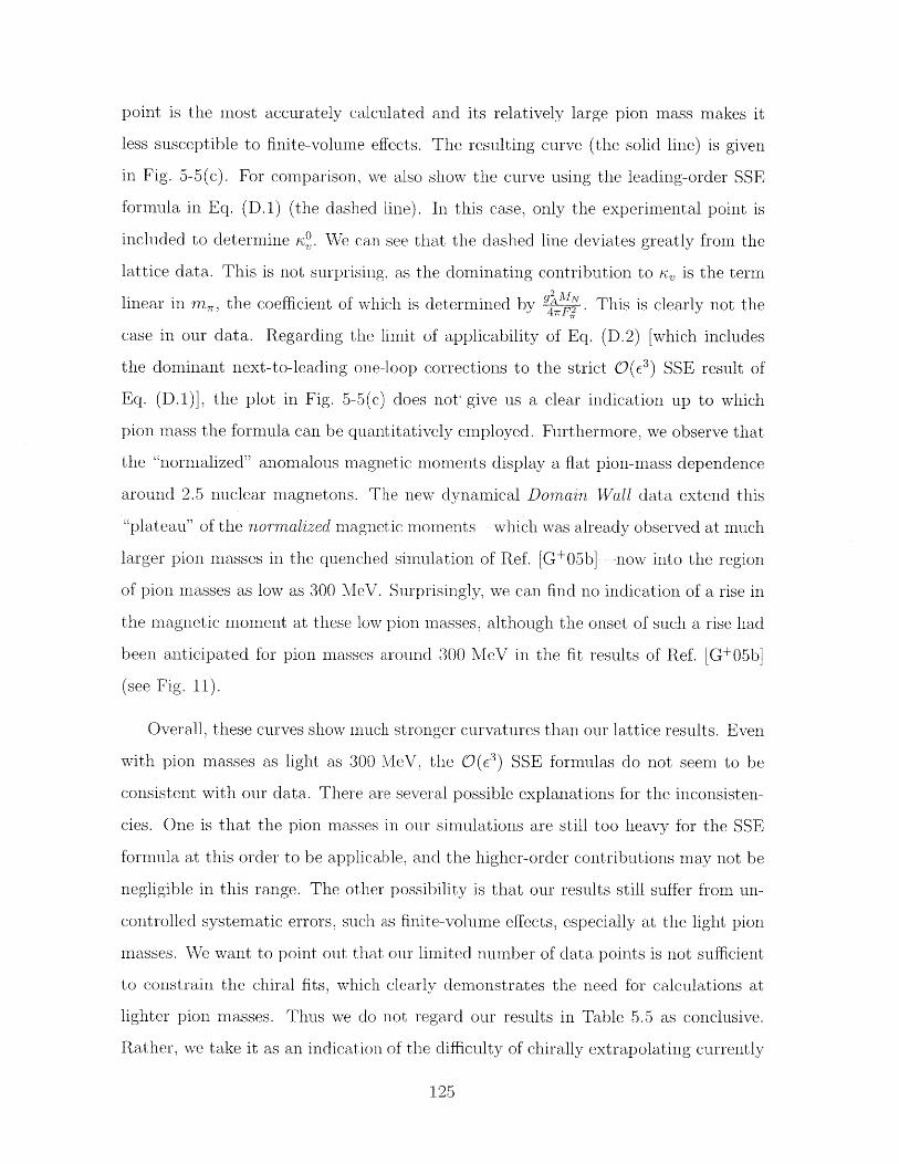
point is the most accurately calculated and its relatively large pion mass makes it
less susceptible to finite-volume effects. The resulting curve (the solid line) is given
in Fig. 5-5(c). For comparison, we also show the curve using the leading-order SSE
formula in Eq. (D.1) (the dashed line). In this case, only the experimental point is
included to determine K<. We can see that the dashed line deviates greatly from the
lattice data. This is not surprising, as the dominating contribution to K. is the term
linear in m, the coefficient of which is determined by . This is clearly not the
case in our data. Regarding the limit of applicability of Eq. (D.2) [which includes
the dominant next-to-leading one-loop corrections to the strict 0(E) SSE result of
Eq. (D.1)], the plot in Fig. 5-5(c) does not give us a clear indication up to which
pion mass the formula can be quantitatively employed. Furthermore, we observe that
the "normalized" anomalous magnetic moments display a flat pion-mass dependence
around 2.5 nuclear magnetons. The new dynamical Domain Wall data extend this
"plateau" of the normalized magnetic moments which was already observed at much
larger pion masses in the quenched simulation of Ref. [G+05b] now into the region
of pion masses as low as 300 MeV. Surprisingly, we can find no indication of a rise in
the magnetic moment at these low pion masses, although the onset of such a rise had
been anticipated for pion masses around 300 MeV in the fit results of Ref. [G+05b]
(see Fig. 11).
Overall, these curves show much stronger curvatures than our lattice results. Even
with pion masses as light as 300 MeV, the 0(E3 ) SSE formulas do not seem to be
consistent with our data. There are several possible explanations for the inconsisten-
cies. One is that the pion masses in our simulations are still too heavy for the SSE
formula at this order to be applicable, and the higher-order contributions may not be
negligible in this range. The other possibility is that our results still suffer from un-
controlled systematic errors, such as finite-volume effects, especially at the light pion
masses. We want to point out that our limited number of data points is not sufficient
to constrain the chiral fits, which clearly demonstrates the need for calculations at
lighter pion masses. Thus we do not regard our results in Table 5.5 as conclusive.
Rather, we take it as an indication of the difficulty of chirally extrapolating currently
125
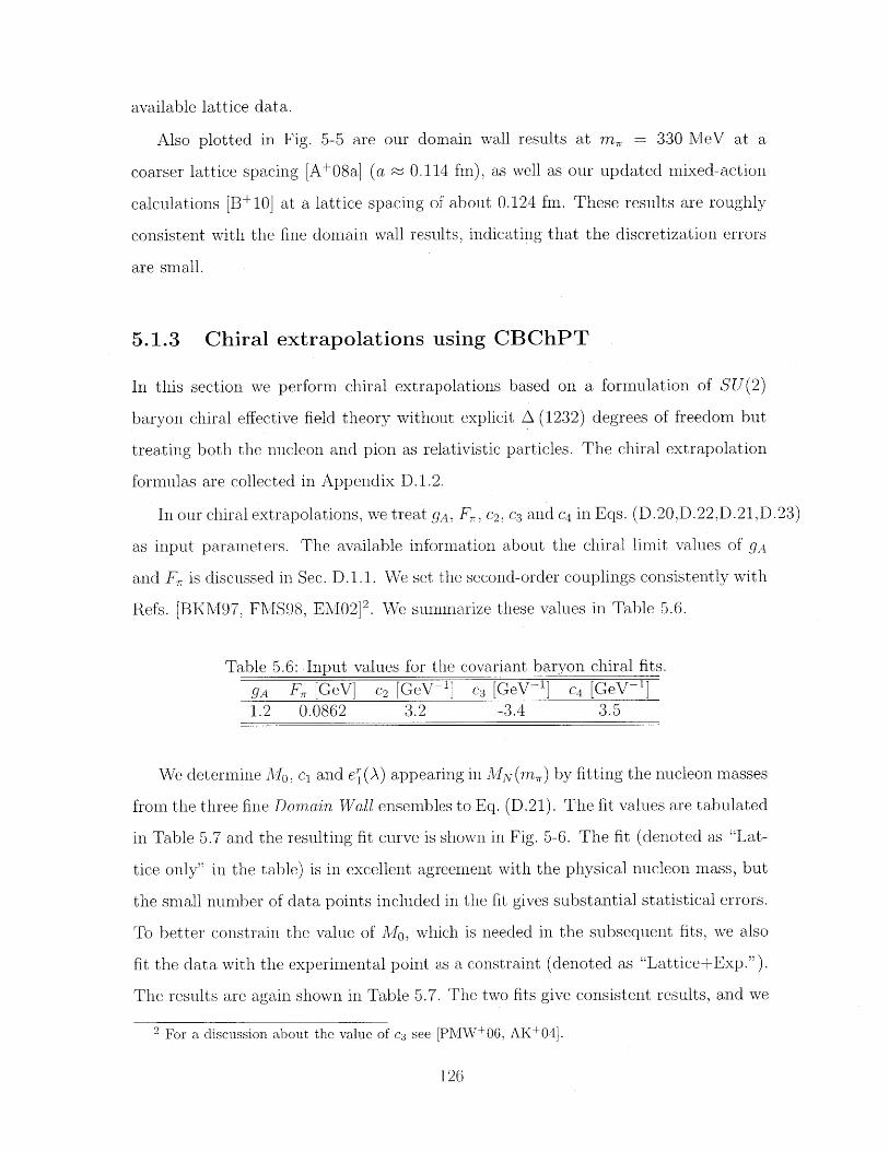
available lattice data.
Also plotted in Fig. 5-5 are our domain wall results at m, = 330 MeV at a
coarser lattice spacing [A+08a) (a ~ 0.114 fm), as well as our updated mixed-action
calculations [B+10] at a lattice spacing of about 0.124 fin. These results are roughly
consistent with the fine domain wall results, indicating that the discretization errors
are small.
5.1.3 Chiral extrapolations using CBChPT
In this section we perform chiral extrapolations based on a formulation of SU(2)
baryon chiral effective field theory without explicit A (1232) degrees of freedom but
treating both the nucleon and pion as relativistic particles. The chiral extrapolation
formulas are collected in Appendix D.1.2.
In our chiral extrapolations, we treat gA, F, c2 , c3 and c4 in Eqs. (D.20,D.22,D.21,D.23)
as input parameters. The available information about the chiral limit values of 9A
and F, is discussed in Sec. D.1.1. We set the second-order couplings consistently with
Refs. [BKM97, FMS98, EM02] 2 . We summarize these values in Table 5.6.
Table 5.6: Input values for the covariant baryon chiral fits.
9A F, [GeV] c2 [GeV-'] c3 [GeV-] c4 [GeV-1]1.2 0.0862 3.2 -3.4 3.5
We determine M10 , ci and ej(A) appearing in M1/,vI(m,) by fitting the nucleon masses
from the three fine Domain Wall ensembles to Eq. (D.21). The fit values are tabulated
in Table 5.7 and the resulting fit curve is shown in Fig. 5-6. The fit (denoted as "Lat-
tice only" in the table) is in excellent agreement with the physical nucleon mass, but
the small number of data points included in the fit gives substantial statistical errors.
To better constrain the value of A10 , which is needed in the subsequent fits, we also
fit the data with the experimental point as a constraint (denoted as "Lattice+Exp.").
The results are again shown in Table 5.7. The two fits give consistent results, and we
2 For a discussion about the value of c3 see [PMW+06, AK+04].
126
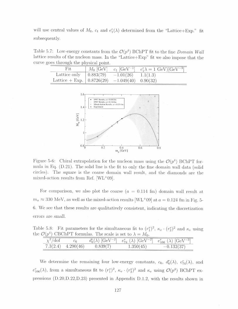
will use central values of MO, ci and er(A) determined from the "Lattice+Exp." fit
subsequently.
Table 5.7: Low-energy constants from the O(p4 ) BChPT fit to the fine Domain Walllattice results of the nucleon mass. In the "Lattice+Exp" fit we also impose that thecurve goes through the physical point.
Fit Mo [GeV] ci [GeV--1] e" A = 1 GeV)([GeV -]Lattice only 0.883(79) -1.01(26) 1.1(1.3)
Lattice + Exp. 0.8726(29) -1.049(40) 0.90(32)
0.2 0.4m, [GeV]
0.6 0.8
Figure 5-6:mula in Eq.
Chiral extrapolation for the nucleon mass using the O(p 4 ) BChPT for-(D.21). The solid line is the fit to only the fine domain wall data (solid
circles). The square is the coarse domain wall result, and the diamonds are themixed-action results from Ref. [WL+09].
For comparison, we also plot the coarse (a = 0.114 fin) domain wall result at
m, a 330 MeV, as well as the mixed-action results [WL+09] at a = 0.124 fin in Fig. 5-
6. We see that these results are qualitatively consistent, indicating the discretization
errors are small.
Table 5.8: Fit parameters for the simultaneous fit to (rz)2 , e- (r")2 and r, usingthe O(p4 ) CBChPT formulas. The scale is set to A = M0 .
2 /dof c d(A) [GeV] e4 (A) [GeV 2 ] e,06 (A) [GeV4]7.3(2.4) 4.290(46) 0.839(7) 1.350(45) -0.132(37)
We determine the remaining four low-energy constants, c6 , dr(A), er4 (A), and
e 06(A), from a simultaneous fit to (rv) 2 , - (r) 2 and v using 0(p 4 ) BChPT ex-
pressions (D.20,D.22,D.23) presented in Appendix D.1.2, with the results shown in
127
1.6
1.4
1. 2
1
I I I I
DWF Results, a - 0.084 fmDWF Results,a 0.I 4Mixed-Action Results, a 0.124 InExperiment
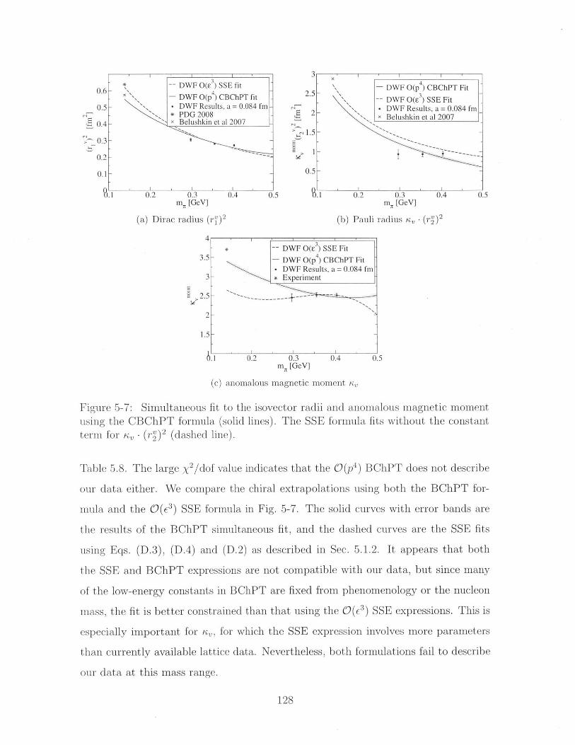
1 13 i
-- DWF O() SSE fit DWF O(p4) CBChPT Fit0.6- 4W (DWF O(p ) CBChPT fit 2.5-- DWF O(E3 ) SSE Fit
0.5- DWF Results, a 0.084 fm - -DWF Results, a = 0.084 fm*PDG 2008 2E
0.4 Belushkin et al 2007 Belushkin et a] 2007
_0.3-
> 0.31
0.21
0.1 0.5
1 0.2 0.3 0.4 0.5 .1 0.2 0.3 0.4 0.5m 7r[GeV) m 71[GeV]
(a) Dirac radius (r' ) 2 (b) Pauli radius K , (r')2
4S-- DWF O(E3) SSE Fit
3.5 - DWF O(p ) CBChPT FitDWF Results, a 0.084 fm
3 * Experiment
2.5 - -----
2-
1.5 -
6.1 0.2 0.3 0.4 0.5m, [GeV]
(c) anomalous magnetic moment K,,
Figure 5-7: Simultaneous fit to the isovector radii and anomalous magnetic momentusing the CBChPT formula (solid lines). The SSE formula fits without the constantterm for K, - (rv) 2 (dashed line).
Table 5.8. The large X2/dof value indicates that the O(p 4 ) BChPT does not describe
our data either. We compare the chiral extrapolations using both the BChPT for-
mula and the 0(E3 ) SSE formula in Fig. 5-7. The solid curves with error bands are
the results of the BChPT simultaneous fit, and the dashed curves are the SSE fits
using Eqs. (D.3), (D.4) and (D.2) as described in Sec. 5.1.2. It appears that both
the SSE and BChPT expressions are not compatible with our data, but since many
of the low-energy constants in BChPT are fixed from phenomenology or the nucleon
mass, the fit is better constrained than that using the 0(6) SSE expressions. This is
especially important for Ko, for which the SSE expression involves more parameters
than currently available lattice data. Nevertheless, both formulations fail to describe
our data at this mass range.
128
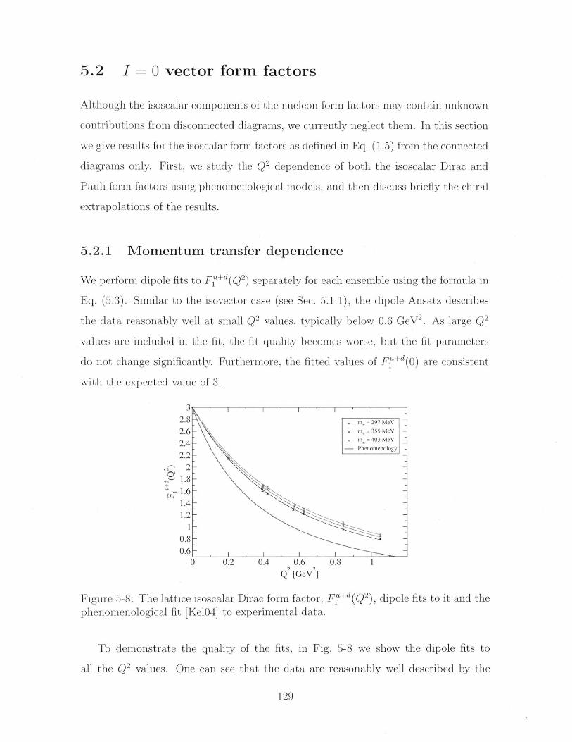
5.2 I = 0 vector form factors
Although the isoscalar components of the nucleon form factors may contain unknown
contributions from disconnected diagrams, we currently neglect them. In this section
we give results for the isoscalar form factors as defined in Eq. (1.5) from the connected
diagrams only. First, we study the Q2 dependence of both the isoscalar Dirac and
Pauli form factors using phenomenological models, and then discuss briefly the chiral
extrapolations of the results.
5.2.1 Momentum transfer dependence
We perform dipole fits to F+d Q 2) separately for each ensemble using the formula in
Eq. (5.3). Similar to the isovector case (see Sec. 5.1.1), the dipole Ansatz describes
the data reasonably well at small Q2 values, typically below 0.6 GeV 2 . As large Q2
values are included in the fit, the fit quality becomes worse, but the fit parameters
do not change significantly. Furthermore, the fitted values of F+d(0) are consistent
with the expected value of 3.
+'
0 0.2 0.4 0.6 0.8 1
Q2 [GeV 2
Figure 5-8: The lattice isoscalar Dirac form factor,phenomenological fit [Kel04] to experimental data.
FT+d(Q 2 ), dipole fits to it and the
To demonstrate the quality of the fits, in Fig. 5-8 we show the dipole fits to
all the Q2 values. One can see that the data are reasonably well described by the
129
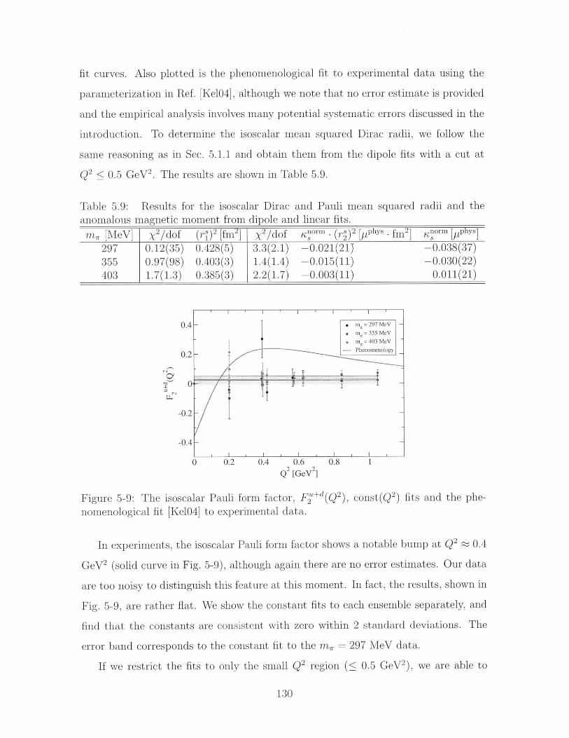
fit curves. Also plotted is the phenomenological fit to experimental data using the
parameterization in Ref. [Ke104], although we note that no error estimate is provided
and the empirical analysis involves many potential systematic errors discussed in the
introduction. To determine the isoscalar mean squared Dirac radii, we follow the
same reasoning as in Sec. 5.1.1 and obtain them from the dipole fits with a cut at
Q2 < 0.5 GeV2 . The results are shown in Table 5.9.
Table 5.9: Results for the isoscalar Dirac and Pauli mean squared radii and theanomalous magnetic moment from dipole and linear fits.
m, [MeV] X2 /dof (rs)2 [fm] X2 /dof r" ""m- (r)2 phys - fmn 3 orm physl
297 0.12(35) 0.428(5) 3.3(2.1) -0.021(21J -0.038(37)355 0.97(98) 0.403(3) 1.4(1.4) -0.015(11) -0.030(22)403 1.7(1.3) 0.385(3) 2.2(1.7) -0.003(11) 0.011(21)
1 T I
0.4- . m = 297 MeV
Sn = 355 MeV
Sm = 403 MeV
Phenomenology0.2 -
-0.2 -
-0.4 --
0 0.2 0.4 0.6 0.8 1
Q [GeV 2]
Figure 5-9: The isoscalar Pauli form factor, F2" d(Q 2), const(Q 2) fits and the phe-
nomenological fit [Ke104] to experimental data.
In experiments, the isoscalar Pauli form factor shows a notable bump at Q2 0.4
GeV 2 (solid curve in Fig. 5-9), although again there are no error estimates. Our data
are too noisy to distinguish this feature at this moment. In fact, the results, shown in
Fig. 5-9, are rather flat. We show the constant fits to each ensemble separately, and
find that the constants are consistent with zero within 2 standard deviations. The
error band corresponds to the constant fit to the m, = 297 MeV data.
If we restrict the fits to only the small Q2 region (< 0.5 GeV 2 ), we are able to
130
perform linear fits to the data and obtain both K - (rs) 2 (from the slope) and K. (from
the intercept), the results of which are also shown in Table 5.93.
5.2.2 Chiral extrapolations using HBChPT+A
As is well known in ChPT (e.g. see the discussion in [BFHM98]), chiral dynamics
in the isoscalar form factors of the nucleon starts at the 3-pion cut, i.e. at two-loop
level, corresponding to 0(c5) in the power-counting of SSE. Hence, the 0(E 3 ) SSE
expressions (D.6) have trivial pion-mass dependence and cannot be used for chiral
extrapolations. Therefore, in this section, we simply extrapolate linearly in m2 the
mean squared Dirac radius to the physical point. This is shown in Fig. 5-10(a), where
we can see that the linear extrapolation gives a result at the physical pion mass which
is much lower than the empirical value. Similarly, we perform a linear extrapolation
for K, . (r-) 2 , which is shown in Fig. 5-10(b).
For K, beyond order E3, additional terms arise including a term linear in the quark
mass. Following Ref. [HW02], we write
Ks = O - 8E 2 MNm2, (5.9)
where K" and £2 are two unknown LECs. This linear dependence describes our data
well, as is shown in Fig. 5-10(c).
5.2.3 Chiral extrapolations using CBChPT
The BChPT formulas up to 0(p 4 ) for (rs)2 , (rs)2 and K,, have also been derived
in [Gai07, GH]. We collect them here for completeness in Appendix D.1.2. We
note, however, that the next-to-leading one-loop BChPT results for the isoscalar
form factors of the nucleon as presented in this section just as in the case of the
leading one-loop SSE-analysis discussed in the previous section do not contain their
dominant chiral dynamics arising from the 3-pion cut. Such effects would only become
3 Like in the isovector case, the anomalous magnetic moment quoted here is normalized to thephysical nuclear magneton according to Eq.(5.8).
131
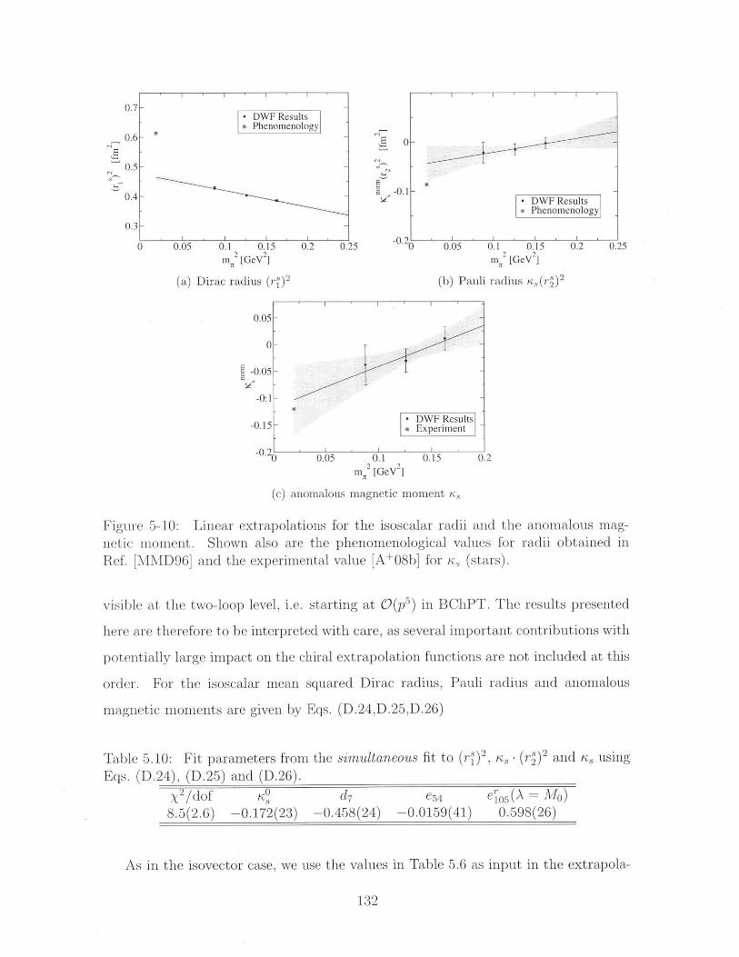
0.05 0.1 0.15m [GeV ]
(a) Dirac radius (r' )2
0.2 0.25 -0.0
m [GeV2
(c) anomalous magnetic moment .,
Figure 5-10:
0.05 0.1 0.15m [GeV 2]
(b) Pauli radius rz@rs)2
SResultsriment
5 0.2
Linear extrapolations for the isoscalar radii and the anomalous mag-netic moment. Shown also are the phenomenological values for radii obtained inRef. [MMD96] and the experimental value [A+08b] for K, (stars).
visible at the two-loop level, i.e. starting at O(p') in BChPT. The results presented
here are therefore to be interpreted with care, as several important contributions with
potentially large impact on the chiral extrapolation functions are not included at this
order. For the isoscalar mean squared Dirac radius, Pauli radius and anomalous
magnetic moments are given by Eqs. (D.24,D.25,D.26)
Table 5.10: Fit parameters from the simultaneous fit to (r) 2 , ,, - (rs)2 and K, usingEqs. (D.24), (D.25) and (D.26).
X2 /dof KO d7 e54 M)8.5(2.6) -0.172(23) -0.458(24) -0.0159(41) 0.598(26)
As in the isovector case, we use the values in Table 5.6 as input in the extrapola-
132
- DWF Results* Phenomenology
*-
DWF Results* Phenomenology _
0.2 0.25
C11
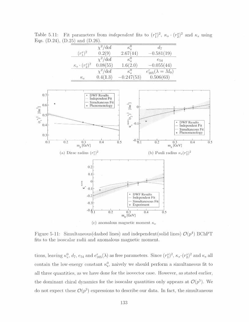
Table 5.11: Fit parameters from independent fitsEqs. (D.24), (D.25) and (D.26).
to (rs) 2 K- (r-) 2 and K8 using
x2 /dof K d(ri)2 0.2(9) 2.67(44) -0.581(19)
X2 /dof K C54S - (if) 2 0.08(55) 1.6(2.0) -0.055(44)
x2 /dof105(el 1-(A Mo)S 0.4(1.3) -0.247(53) 0.506(63)
0.2 0.3mE [GeV]
(a) Dirac radius (r") 2
0.2-
0.1
0-
-0.1 -
-0.2
-0.3_
-0.
(c)
0.4 0
0
-0.1
.5 -0; .1
I I I
-
- DWF ResultsIndependent FitSimultanesous Fit
* Experiment
0.2 0.3 0.4 0m [GeV]
anomalous magnetic moment K,
* rhenomenology
0.2 0.3 0.4 0.5m, [GeV]
(b) Pauli radius aS) 2
Figure 5-11: Simultaneous (dashed lines) and independent (solidfits to the isoscalar radii and anomalous magnetic moment.
lines) O(p4 ) BChPT
tions, leaving i0, d7 , e5 4 and eL 5 (A) as free parameters. Since (rs)2 , -(?-)2 and is all
contain the low-energy constant i, naively we should perform a simultaneous fit to
all three quantities, as we have done for the isovector case. However, as stated earlier,
the dominant chiral dynamics for the isoscalar quantities only appears at O(p 5 ). We
do not expect these O(ps) expressions to describe our data. In fact, the simultaneous
133
0.7
0.6C E
0.5
0.4
0.3
0.
DWF ResultsIndependent Fit
- Simultaneous Fit* Phenomenology
- - -- -- ---- ~----- - - - - -* - DWF Results
- Independent Fit--- Simultaneous Fit
I
fit to these three quantities gives a X2/dof of about 9 (see Table 5.10), showing the
difficulty in fitting these quantities consistently. Looking closely at each quantity
separately, we find that independent fits to (rK2 , s- (rs) 2 and /, lead to an incon-
sistency in the estimation of the common parameter r<, as shown in Table 5.11. For
demonstrative purposes, we compare the resulting fit curves from the simultaneous
fit and the independent fits in Fig. 5-11, from which we see that the independent fits
provide reasonable extrapolations for the data, while the simultaneous fit misses the
data points badly, indicating inconsistencies of the BChPT expressions at this order.
We also note that the extrapolated value for (rs)2 at the physical pion mass is about
20% lower than the phenomenological value. These observations lead us to conclude
that the BChPT expressions at 0(p 3) are not applicable in the pion-mass range of our
calculation. Of course, since we have not included the disconnected diagrams in our
calculations, there are uncontrolled systematic errors which may also affect the pion-
mass dependence. Further investigations are required to draw definitive conclusions
for these isoscalar quantities.
5.3 Axial form factors
5.3.1 Axial charge
The nucleon axial charge is an important phenomenological quantity, which, for ex-
ample, determines the rate of the neutron /-decay (see Sec. 1.2). The lattice axial
current operator [q-y,' 5q] must be renormalized, and the renormalization procedure
for Wilson-clover quarks is different from that for domain wall quarks. We have not
renormalized the axial current. However, we can study the ratios in which the renor-
malization constant cancels to extract, for example, the axial radius in Section 5.3.2.
In order to compare our three calculations, in Figure 5-12 we show the ratio of
the nucleon axial charge to the pion decay constant gA/F, in which the axial current
renormalization ZA is canceled. The values for F, are taken from Ref. [col]. On a
small panel within Fig. 5-12 we show the ratio gA/gv that will give the renormalized
134
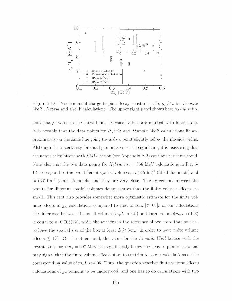
1.2 -3 .
0 0.2 0.4 m_8-
7- Hybrid a=0.124 fm0 Domain Wall a=0.084 fm
BMW 24 *48
BMW 32 *48
1.1 0.2 0.3 0.4 0.5 0.6m, [GeV]
Figure 5-12: Nucleon axial charge to pion decay constant ratio, gA/F, for DomainWall , Hybrid and BMW calculations. The upper right panel shows bare gA/gv ratio.
axial charge value in the chiral limit. Physical values are marked with black stars.
It is notable that the data points for Hybrid and Domain Wall calculations lie ap-
proximately on the same line going towards a point slightly below the physical value.
Although the uncertainty for small pion masses is still significant, it is reassuring that
the newer calculations with BMW action (see Appendix A.3) continue the same trend.
Note also that the two data points for Hybrid m, 356 MeV calculations in Fig. 5-
12 correspond to the two different spatial volumes, (2.5 fm) 3 (filled diamonds) and
(3.5 fm)3 (open diamonds) and they are very close. The agreement between the
results for different spatial volumes demonstrates that the finite volume effects are
small. This fact also provides somewhat more optimistic estimate for the finite vol-
ume effects in gA calculations compared to that in Ref. [Y+09]: in our calculations
the difference between the small volume (mL 4.5) and large volume(m , L ~~ 6.3)
is equal to ~~ 0.006(22), while the authors in the reference above state that one has
to have the spatial size of the box at least L > 6m; 1 in order to have finite volume
effects ,< 1%. On the other hand, the value for the Domain Wall lattice with the
lowest pion mass n , = 297 MeV lies significantly below the heavier pion masses and
may signal that the finite volume effects start to contribute to our calculations at the
corresponding value of mL ~ 4.05. Thus, the question whether finite volume affects
calculations of 9A remains to be understood, and one has to do calculations with two
135

different volumes at the same small pion mass to do a direct comparison.
0.2 0.3 0.4 0.5m, [GeV]
(a) Hybrid data extrapolation
1.4
1.3
S1.2
1.1
. i . 2.7 T .DWJ3-pararn HBChPT JDW1I IHybrid (2.5 fmi) I
--- -2param HBChPT [Hy].3-pararn HBChPTr tHy
0.2 0.3 0.4m. [GeV]
(b) Domain Wall data extrapolation
Figure 5-13: Chiral extrapolations of the nucleon axial charge for the Domain Walland Hybrid calculations. In the two-parameter HBChPT fit gi = 2.5 is set.
The renormalized gA results enable a direct comparison between Hybrid and Do-
main Wall calculations. In Figure 5-13 we show data for both ensembles and perform
a chiral extrapolation using the HBChPT prediction [HPW03]
gA (rr27 ) = 9A - A6w2 +1 7T
4m 2{fC(A)C2
+ CA 155 g1- L7g ]227 2 3
+ 7log 9 + AcgA 8cgm2 [1
277F A 277r2F
+ 81i2 F2 (25g,272
- 57gA){ log
where y = 16r 2F 1
Mn2 1
- ] log R(m)
-log R(m,,)M, A2
2 1 - 2 3cAg1 -gA - ca9g -A
The choice for the chiral limit parameters F1., A = mA - MN, CA = 9 7rNA is
discussed in Sec. D.1.1. In addition, to perform the fits, we have to fix
CA = 1.5,
for a three-parameter fit and also
9g = 2.5 -9A
5[quark-flavor symmetry]
136
0.5 0.6
(5.10)
for a two-parameter fit. The only remaining parameters are the chiral limit value
g A the counterterm C(A). The two-parameter fit is more reliable because there are
data only three distinct values of m, < 500 MeV in both Domain Wall and Hybrid
calculations, and applying the HBChPT+A formula for m, > 500 MeV is question-
able. From the two-parameter fits we extract the values of extrapolated axial charge
9A (m, ~ 140 MeV),
phys 1.160(14) [Hybrid ],
gA4hys = 1.139(20) [Domain Wall ],
in our two calculations. Both results underestimate the experimental value 9A
1.126(3). This disagreement may be the result of the following:
1. heavy pion mass data points used for chiral extrapolations,
2. insufficient order of approximation in HBChPT+A
3. finite-volume effects contributing to the lightest pion mass valuesm, - 300 MeV,
to which the chiral extrapolations are most sensitive.
5.3.2 Momentum transfer dependence
From our lattice calculations we can also extract dependence of the nucleon axial
form factors on the momentum transfer Q2. Currently, the form factor results only
for the Domain Wall and Hybrid calculations are available, because additional work
to renormalize the axial current in the BMW calculation is required.
In Figure 5-14 we show our results for the GA form factor from both Domain
Wall and Hybrid calculations with the two lightest pion masses approximately equal
to m , = 300 and 350 MeV. Additionally, we show the results for the second (larger)
volume V - (3.5 fm) 3 from Hybrid lattice with m, = 350 MeV, which indicate no
noticeable difference from the other (smaller) volume V e (2.5 fm) 3. This agreement
demonstrates that the finite volume effects are small and negligible at our current
137
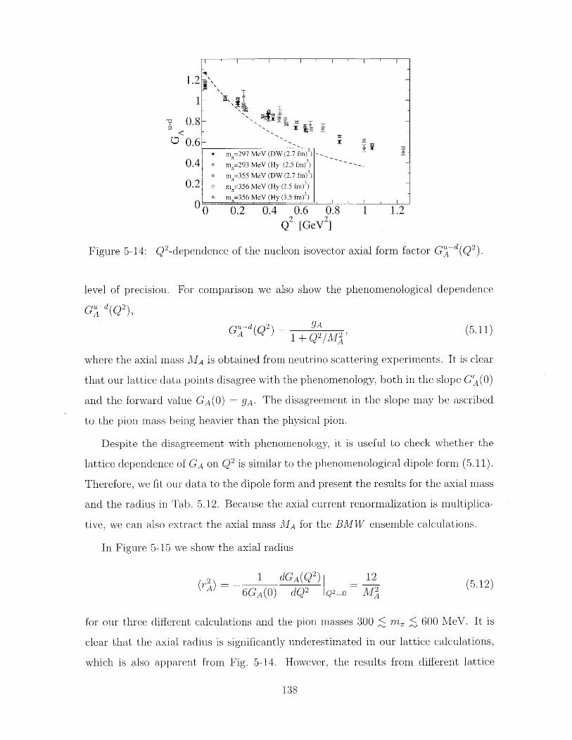
1.2-
1
- 0.8 -
0.6 -m 7=297 MeV (DW (2.7 fm)3)
0.4 40m =293 MeV (Hy (2.5 fm)3 )
n=355 MeV (DW (2.7 fm) )0.2 m 7=356 MeV (Hy (2.5 fm)3)
m m =356 MeV (Hy (3.5 fm)3)
0 0.2 0.4 0.6 0.8 1 1.2
Q 2[GeV2
Figure 5-14: Q2 -dependence of the nucleon isovector axial form factor GA-dQ2
level of precision. For comparison we also show the phenomenological dependence
GG )d(Q2),
G"~d(Q2) 9A (5.11)A 1 _+ Q2/My2
where the axial mass MA is obtained from neutrino scattering experiments. It is clear
that our lattice data points disagree with the phenomenology, both in the slope G' (0)
and the forward value GA(0) = YA. The disagreement in the slope may be ascribed
to the pion mass being heavier than the physical pion.
Despite the disagreement with phenomenology, it is useful to check whether the
lattice dependence of GA on Q2 is similar to the phenomenological dipole form (5.11).
Therefore, we fit our data to the dipole form and present the results for the axial mass
and the radius in Tab. 5.12. Because the axial current renormalization is multiplica-
tive, we can also extract the axial mass MA for the BMW ensemble calculations.
In Figure 5-15 we show the axial radius
Kr2 - 1 dGA(Q 2) 126GA(0) dQ 2 Q2=0 M(
for our three different calculations and the pion masses 300 < m, < 600 MeV. It is
clear that the axial radius is significantly underestimated in our lattice calculations,
which is also apparent from Fig. 5-14. However, the results from different lattice
138
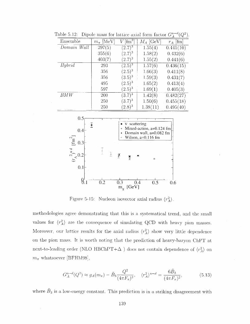
Ensemble M, [MeV] V [fm 3] MA [GeV] rA [fin]Domain Wall 297(5) (2.7) 3 1.55(4) 0.441(10)
355(6) (2.7)3 1.58(2) 0.432(6)403(7) (2.7)3 1.55(2) 0.441(6)
Hybrid 293 (2.5)3 1.57(6) 0.436(15)
356 (2.5)3 1.66(3) 0.411(8)356 (3.5)3 1.59(3) 0.431(7)495 (2.5 )3 1.65(2) 0.413(4)597 (2.5)3 1.69(1) 0.405(3)
BMW 200 (3.7)3 1.42(8) 0.482(27)250 (3.7)3 1.50(6) 0.455(18)250 (2.8)3 1.38(11) 0.495(40)
0.51 1 1 1
0.2 0.3 0.4m1 [GeV]
0.5 0.6
Figure 5-15: Nucleon isovector axial radius (r2).
methodologies agree demonstrating that this is a systematical trend, and the small
values for (r2) are the consequence of simulating QCD with heavy pion masses.
Moreover, our lattice results for the axial radius (r2) show very little dependence
on the pion mass. It is worth noting that the prediction of heavy-baryon ChPT at
next-to-leading order (NLO HBChPT+A ) does not contain dependence of (r 2) on
m, whatsoever [BFHM98],
Q2GAd(Q2) yA rrbr) - 53 (47F,)2 1
where B 3 is a low-energy constant. This prediction is in a striking disagreement with
139
0.4 Hrl
*v scattermngMixed-action, a=0.124 fm
. Domain wall, a=0.082 fmWilson, a=0.116 fm
JE 3-
0.3-
0.2
0.1-
lattice axial form factor G'-d(Q2).Table 5.12: Dipole mass for
gi__
0.1
65f3a -e ,(5.13)rA )u
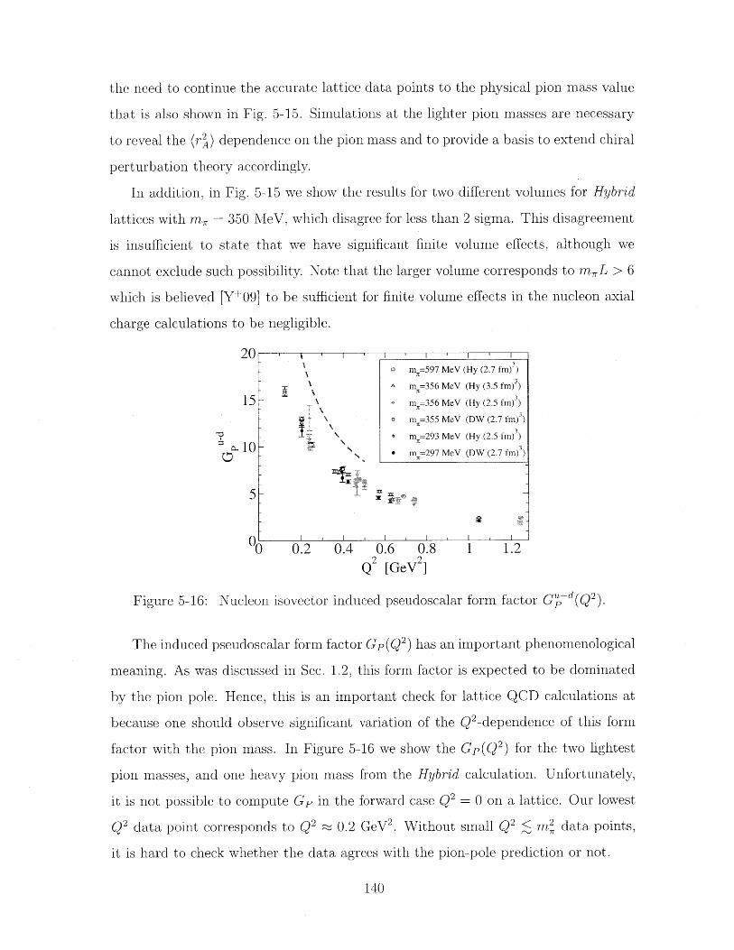
the need to continue the accurate lattice data points to the physical pion mass value
that is also shown in Fig. 5-15. Simulations at the lighter pion masses are necessary
to reveal the (r' dependence on the pion mass and to provide a basis to extend chiral
perturbation theory accordingly.
In addition, in Fig. 5-15 we show the results for two different volumes for Hybrid
lattices with m, = 350 MeV, which disagree for less than 2 sigma. This disagreement
is insufficient to state that we have significant finite volume effects, although we
cannot exclude such possibility. Note that the larger volume corresponds to mL > 6
which is believed [Y+09] to be sufficient for finite volume effects in the nucleon axial
charge calculations to be negligible.
20m,,=597 MeV (Hy (2.7 fm) )
m =356 MeV (Hy (3.5 fm) )
15 m =356 MeV (Hy (2.5 fm) )
m =355 MeV (DW (2.7 fm) )
7)+ m =293 MeV (Hy (2.5 fm) )
10 em =297 MeV (DW (2.7 fm) )
5 -
0 0 0.2 0.4 0.6 0.8 1 1.2
Q2 [GeV2]
Figure 5-16: Nucleon isovector induced pseudoscalar form factor G- d(Q2)
The induced pseudoscalar form factor Gp(Q 2) has an important phenomenological
meaning. As was discussed in Sec. 1.2, this form factor is expected to be dominated
by the pion pole. Hence, this is an important check for lattice QCD calculations at
because one should observe significant variation of the Q2-dependence of this form
factor with the pion mass. In Figure 5-16 we show the Gp(Q 2 ) for the two lightest
pion masses, and one heavy pion mass from the Hybrid calculation. Unfortunately,
it is not possible to compute G in the forward case Q2 = 0 on a lattice. Our lowest
Q2 data point corresponds to Q2 ~ 0.2 GeV 2 . Without small Q2 ,< M data points,
it is hard to check whether the data agrees with the pion-pole prediction or not.
140
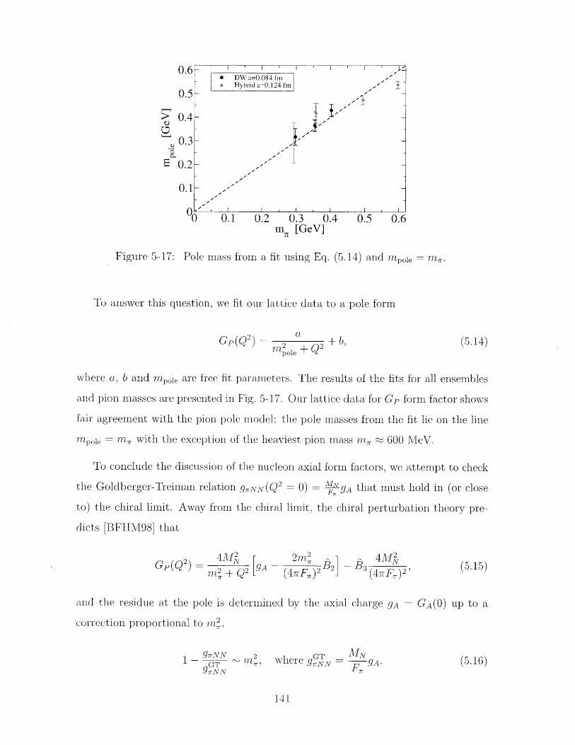
0.1 0.2 0.3 0.4m, [GeV]
Figure 5-17: Pole mass from a fit using Eq. (5.14) and mnpole = mr .
To answer this question, we fit our lattice data to a pole form
Gp (Q2) = 2 + 2 + ,mpoie+Q
(5.14)
where a, b and mpole are free fit parameters. The results of the fits for all ensembles
and pion masses are presented in Fig. 5-17. Our lattice data for Gp form factor shows
fair agreement with the pion pole model: the pole masses from the fit lie on the line
Rpole = m, with the exception of the heaviest pion mass in, ~ 600 MeV.
To conclude the discussion of the nucleon axial form factors, we attempt to check
the Goldberger-Treiman relation 9,NN (Q 2 - 0) 9 MN 9A that must hold in (or close
to) the chiral limit. Away from the chiral limit, the chiral perturbation theory pre-
dicts [BFHM98] that
Gp(Q 2) 4 9A -M2 + Q2 -
2m 2 ~(4 17r, )2 2
~ 4M2(47rF,)2-
and the residue at the pole is determined by the axial charge gA = GA(0) up to a
correction proportional to m1i,
9NN 2GT ~
9 , NN
where gGT MNrNN F,9A
141
0.6
0.5K
>0.4-
0.3-
3 0.2 -
0.1-
0-0
* DW a=0.084 frn+ Hybrid a=O.124 fm
S, I , I . I .
0.5 0.6
(5.15)
(5.16)
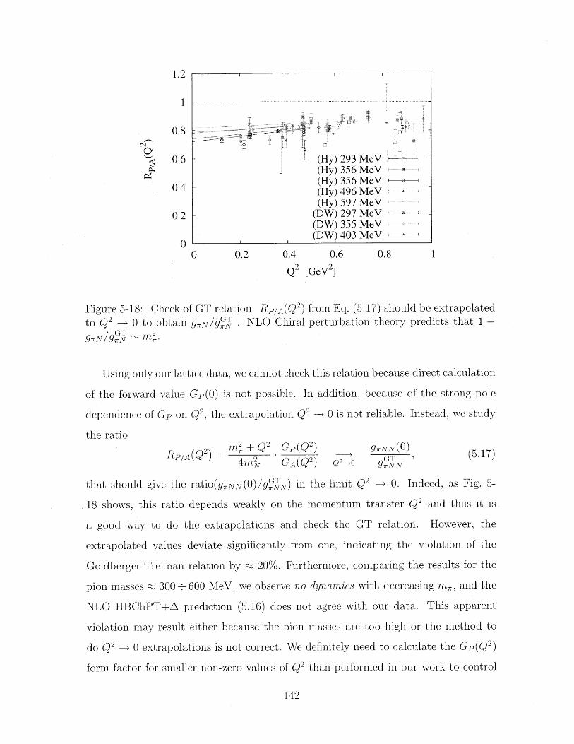
1.2
1 -
0.8CI
0.6 (Hy) 293 MeV(Hy) 356 MeV(Hy) 356 MeV
0.4 - (Hy) 496 MeV(Hy) 597 MeV
0.2 (DW) 297 MeV(DW) 355 MeV
0 ' (DW? 403 MeV
0 0.2 0.4 0.6 0.8 1
Q2 [GeV2
Figure 5-18: Check of GT relation. RPIA(Q 2 ) from Eq. (5.17) should be extrapolated
to Q2 - 0 to obtain gr9NTg . NLO Chiral perturbation theory predicts that 1 -rr7rN
9 rN ,/r
Using only our lattice data, we cannot check this relation because direct calculation
of the forward value Gp(0) is not possible. In addition, because of the strong pole
dependence of Gp on Q2, the extrapolation Q2 -> 0 is not reliable. Instead, we study
the ratiom2 + Q2 Gp(Q 2) 9,rNN (0)
RP/A (Q2) 7TT2 (Q)Q,)0 GT ,(5.17)4N GA(Q 2 ) Q0 9,rNN
that should give the ratio(grNN 9NjTN) in the limit Q2 -+ 0. Indeed, as Fig. 5-
18 shows, this ratio depends weakly on the momentum transfer Q2 and thus it is
a good way to do the extrapolations and check the GT relation. However, the
extrapolated values deviate significantly from one, indicating the violation of the
Goldberger-Treiman relation by ~ 20%. Furthermore, comparing the results for the
pion masses ~ 300 + 600 MeV, we observe no dynamics with decreasing mr, and the
NLO HBChPT+A prediction (5.16) does not agree with our data. This apparent
violation may result either because the pion masses are too high or the method to
do Q2 -- 0 extrapolations is not correct. We definitely need to calculate the Gp(Q 2)
form factor for smaller non-zero values of Q2 than performed in our work to control
142
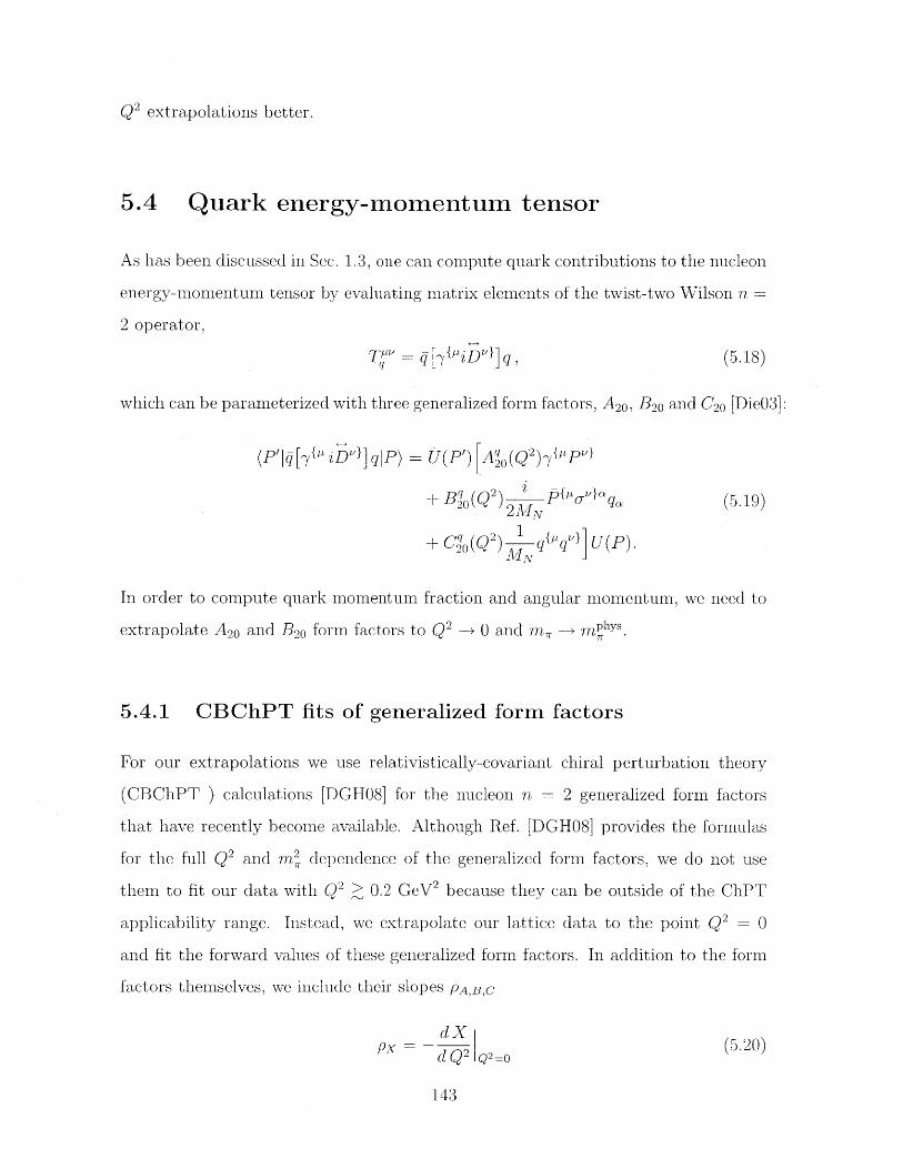
Q2 extrapolations better.
5.4 Quark energy-momentum tensor
As has been discussed in Sec. 1.3, one can compute quark contributions to the nucleon
energy-momentum tensor by evaluating matrix elements of the twist-two Wilson n=
2 operator,
Ta' = g[7}{iDiI]q, (5.18)
which can be parameterized with three generalized form factors, A 20 , B 20 and C20 [Die03]:
(P'q[7y{ iD] qlP) = U(P') FA O(Q2);{Pp
+ Bq (Q2) z" f/ "a (5.19)2MN
+ Ci (Qq2) q'j U(P).MN
In order to compute quark momentum fraction and angular momentum, we need to
extrapolate A 2 0 and B 20 form factors to Q2 -+ 0 and m,_ -_ mphys
5.4.1 CBChPT fits of generalized form factors
For our extrapolations we use relativistically-covariant chiral perturbation theory
(CBChPT ) calculations [DGH08] for the nucleon n = 2 generalized form factors
that have recently become available. Although Ref. [DGH08] provides the formulas
for the full Q2 and m2 dependence of the generalized form factors, we do not use
them to fit our data with Q2 > 0.2 GeV 2 because they can be outside of the ChPT
applicability range. Instead, we extrapolate our lattice data to the point Q2 = 0
and fit the forward values of these generalized form factors. In addition to the form
factors themselves, we include their slopes pA,B,c
dXpOX = - (5.20)
d Q2 Q2=0
143
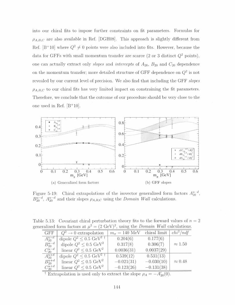
into our chiral fits to impose further constraints on fit parameters. Formulas for
PA,B,c are also available in Ref. [DGH08]. This approach is slightly different from
Ref. [B+10] where Q2 # 0 points were also included into fits.. However, because the
data for GFFs with small momentum transfer are scarce (2 or 3 distinct Q2 points),
one can actually extract only slopes and intercepts of A20 , B 20 and C20 dependence
on the momentum transfer; more detailed structure of GFF dependence on Q2 is not
revealed by our current level of precision. We also find that including the GFF slopes
PA,B,C to our chiral fits has very limited impact on constraining the fit parameters.
Therefore, we conclude that the outcome of our procedure should be very close to the
one used in Ref. [B+10].
0.3
0.2
0.1
0
0.1 0.2 0.3 0.4m [GeV]
0.5 0.6
(a) Generalized form factors
Figure 5-19:
(b) GFF slopes
Chiral extrapolations of the isovector generalized form factors A2d"Bu-d, A2od and their slopes PA,B,c using the Domain Wall calculations.
Table 5.13: Covariant chiral perturbation theory fits to the forward values of n= 2generalized form factors at t2 = (2 GeV) 2 , using the Domain Wall calculations.
GFF Q2 - 0 extrapolation n, = 140 MeV chiral limit chi 2 /ndfAQ220 dipole Q2 <0.5 GeV2 t 0.204(6) 0.177(6)
B- dipole Q2 < 0.5 GeV 2 0.317(8) 0.306(7) 1.50
C2o-d linear Q2 < 0.5 GeV 2 0.0036(31) 0.0037(29)A2"ojd dipole Q2 < 0.5 GeV 2 t 0.539(12) 0.531(13)
B20jd linear Q2 < 0.5 GeV 2 -0.021(31) -0.030(10) 0.48
C0jd linear Q2 < 0.5 GeV2 -0.123(26) -0.131(38)
i Extrapolation is used only to extract the slope PA = -A'20(0).
144
A A
-
-
- -
0 01 02 03 040.5 0.
0.4- m+CoAm
0.3 - + B0
0.2--
0.1-
-0.10 0.1 0.2 0.3 0.4 0.5 0.6
mR [GeV]
Figure 5-20: Chiral extrapolations of the isoscalar generalized form factors A,+d,Bljd, Agjd using the Domain Wall calculations.
To extrapolate the GFFs to the point Q2 = 0, we use a dipole form and switch to
a linear form for form factors that are close to zero. The methods used in each case
are listed in Tab. 5.13. Best fit curves to A'a~d(Q 2 ), B td(Q 2 ) and CoId(Q2) data
are shown in Fig. 5-29 and Fig. 5-30 for the Domain Wall and Hybrid calculations,
respectively. The dependence of the Q2 -- 0 extrapolated values on fit forms used is
not significant, because the estimated uncertainties of the data points are dominated
by their stochastic variations.
We perform a simultaneous fit to the isovector generalized form factors A'-~d, B- d
and C2- d and their slopes PA,B,C using Eq. (28,31,32) and Eq. (34-36) of Ref. [DGH08],
which include the 0(p2 ) terms in the effective Lagrangian. In addition, these formulas
include terms that "estimate" 0(p3) corrections. Our numerical analysis shows that
these terms are important, in agreement with the results in Ref.[DGH08]. We fix
the value of the parameter Aao = 0.165, which is known from the analysis of other
lattice data [E+06a], and the other 8 fit parameters
a'U,0, b2",o, c,O, C7, )C12, 6t, oI 6 o , (5.21)Sf h r oA B C
are free. The results of the fits to the Domain Wall data are shown in Fig. 5-19. In
145
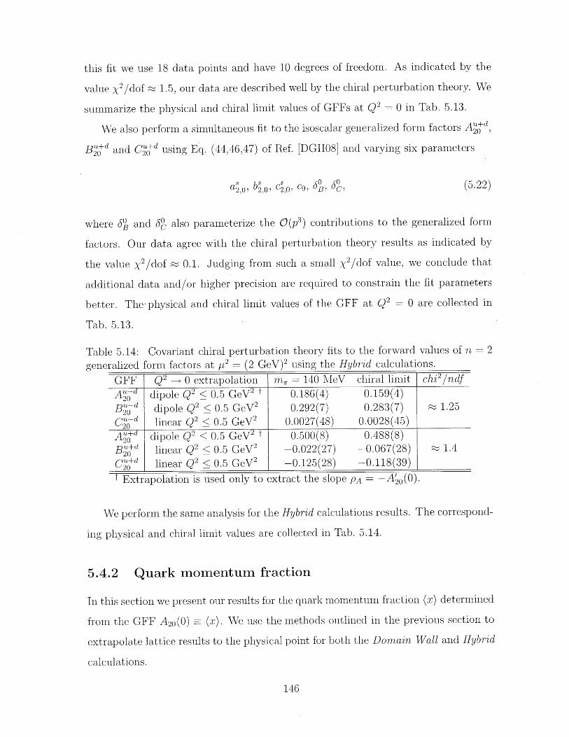
this fit we use 18 data points and have 10 degrees of freedom. As indicated by the
value x 2 /dof a 1.5, our data are described well by the chiral perturbation theory. We
summarize the physical and chiral limit values of GFFs at Q2 = 0 in Tab. 5.13.
We also perform a simultaneous fit to the isoscalar generalized form factors A"d,
Bujd and Cojd using Eq. (44,46,47) of Ref. [DGH08] and varying six parameters
as, , bs0, c0 , c9, o0, 60, (5.22)
where 60 and o' also parameterize the 0(p 3 ) contributions to the generalized form
factors. Our data agree with the chiral perturbation theory results as indicated by
the value X2/dof ~ 0.1. Judging from such a small X2 /dof value, we conclude that
additional data and/or higher precision are required to constrain the fit parameters
better. The physical and chiral limit values of the GFF at Q2 - 0 are collected in
Tab. 5.13.
Table 5.14: Covariant chiral perturbation theory fits to the forward values of n 2
generalized form factors at t 2 = (2 GeV)2 using the Hybrid calculations.
GFF Q2 - 0 extrapolation m, = 140 MeV chiral limit chi 2 /nqf
A20 7 7 dipole Q2 < 0.5 GeV2 t 0.186(4) 0.159(4)
B0u-d dipole Q2 < 0.5 GeV 2 0.292(7) 0.283(7) 1.25
C20ud linear Q2 < 0.5 GeV 2 0.0027(48) 0.0028(45)
A2"fd dipole Q2 < 0.5 GeV 2 t 0.500(8) 0.488(8)B f linear Q2 < 0.5 GeV 2 -0.022(27) -0.067(28) 1.4
Cujd linear Q2 < 0.5 GeV 2 -0.125(28) -0.118(39)
t Extrapolation is used only to extract the slope PA = -A'(0).
We perform the same analysis for the Hybrid calculations results. The correspond-
ing physical and chiral limit values are collected in Tab. 5.14.
5.4.2 Quark momentum fraction
In this section we present our results for the quark momentum fraction (x) determined
from the GFF A 20 (0) (4 We use the methods outlined in the previous section to
extrapolate lattice results to the physical point for both the Domain Wall and Hybrid
calculations.
146
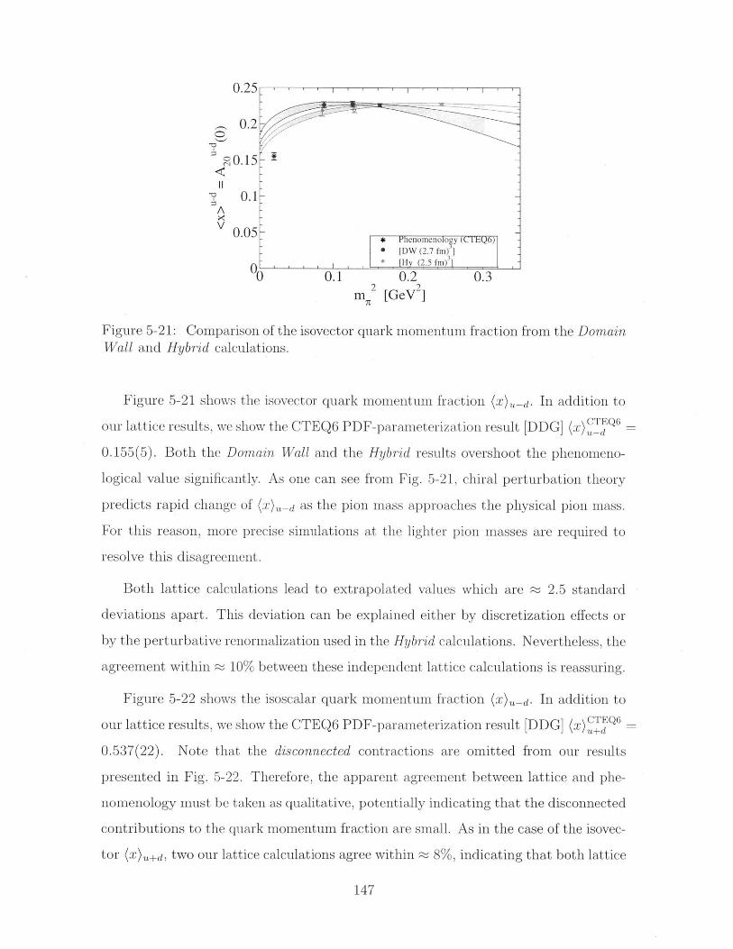
0.2
0.2 -
0.15 -
- 0.1 -A
v 0.05* henomenolg (02y Q
. [DW (2.7 fi)]
0 [Hy (2.5 fn)'-
0 0.1 0.2 0.3m [GeV2
Figure 5-21: Comparison of the isovector quark momentum fraction from the DomainWall and Hybrid calculations.
Figure 5-21 shows the isovector quark momentum fraction (x)ud. In addition to
our lattice results, we show the CTEQ6 PDF-parameterization result [DDG] (X)_TQ6 -
0.155(5). Both the Domain Wall and the Hybrid results overshoot the phenomeno-
logical value significantly. As one can see from Fig. 5-21, chiral perturbation theory
predicts rapid change of (x)ud as the pion mass approaches the physical pion mass.
For this reason, more precise simulations at the lighter pion masses are required to
resolve this disagreement.
Both lattice calculations lead to extrapolated values which are a 2.5 standard
deviations apart. This deviation can be explained either by discretization effects or
by the perturbative renormalization used in the Hybrid calculations. Nevertheless, the
agreement within - 10% between these independent lattice calculations is reassuring.
Figure 5-22 shows the isoscalar quark momentum fraction (x)ud. In addition to
our lattice results, we show the CTEQ6 PDF-parameterization result [DDG] (x) + 6
0.537(22). Note that the disconnected contractions are omitted from our results
presented in Fig. 5-22. Therefore, the apparent agreement between lattice and phe-
nomenology must be taken as qualitative, potentially indicating that the disconnected
contributions to the quark momentum fraction are small. As in the case of the isovec-
tor (x)u+d, two our lattice calculations agree within ~ 8%, indicating that both lattice
147
5-
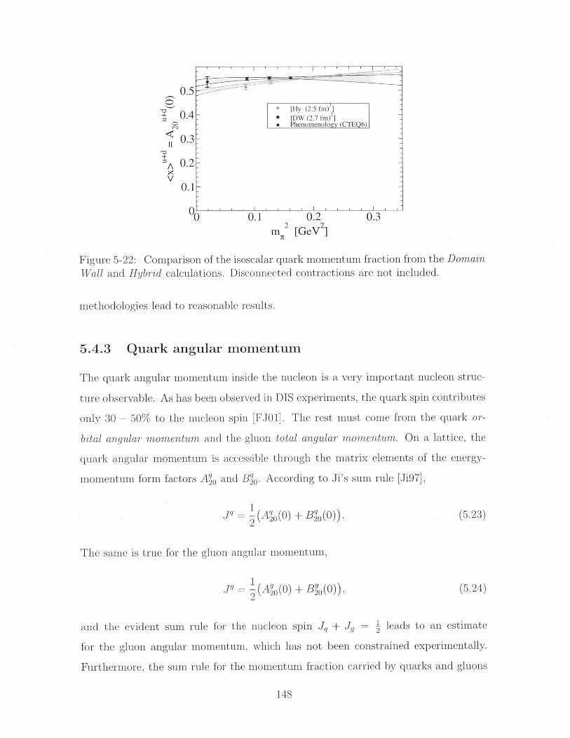
0.5
+ 0.4
0.3
A 0.2V
0.1
0 0.1 0.2 0.3
m 2 [GeV2
Figure 5-22: Comparison of the isoscalar quark momentum fraction from the Domain
Wall and Hybrid calculations. Disconnected contractions are not included.
methodologies lead to reasonable results.
5.4.3 Quark angular momentum
The quark angular momentum inside the nucleon is a very important nucleon struc-
ture observable. As has been observed in DIS experiments, the quark spin contributes
only 30 - 50% to the nucleon spin [FJ01]. The rest must come from the quark or-
bital angular momentum and the gluon total angular momentum. On a lattice, the
quark angular momentum is accessible through the matrix elements of the energy-
momentum form factors A' 0 and B' . According to Ji's sum rule [Ji97],
1jq - (A qo(0) + B q(0)). (5.23)
2 22
The same is true for the gluon angular momentum,
1Jg - (Ago (0) + Bg (0)), (5.24)
2 22
and the evident sum rule for the nucleon spin Jq + Jg = leads to an estimate
for the gluon angular momentum, which has not been constrained experimentally.
Furthermore, the sum rule for the momentum fraction carried by quarks and gluons
148
[Hy (2.5 fm)]* [DW (2.7 fm)~]* Phenomenology (CTEQ6)
SI , , I I
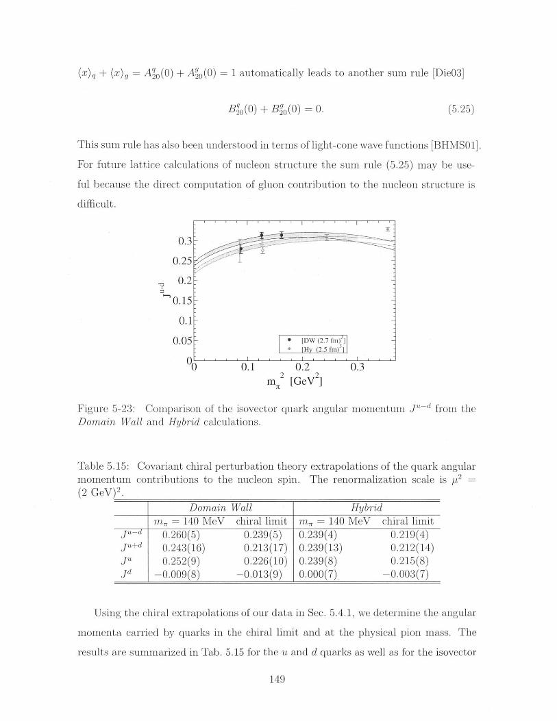
(X)q + (X) = A 0 (0) + A' 0 (0) = 1 automatically leads to another sum rule [Die03]
Bjo(0) + Bg (0) = 0. (5.25)
This sum rule has also been understood in terms of light-cone wave functions [BHMSO1).
For future lattice calculations of nucleon structure the sum rule (5.25) may be use-
ful because the direct computation of gluon contribution to the nucleon structure is
difficult.
0.3
0.25
0.2
0.15
0.1
0.05
0.1 0.22 [GeV2
0.3
Figure 5-23:Domain Wall
Comparison of the isovector quark angular momentum Ju-d from theand Hybrid calculations.
Table 5.15: Covariant chiral perturbation theory extrapolations of themomentum contributions to the nucleon spin. The renormalization
quark angularscale is p2
(2 GeV) 2 .
Domain Wall Hybridm, = 140 MeV chiral limit m, = 140 MeV chiral limit
J"--d 0.260(5) 0.239(5) 0.239(4) 0.219(4)ju+d 0.243(16) 0.213(17) 0.239(13) 0.212(14)J"t 0.252(9) 0.226(10) 0.239(8) 0.215(8)Jd -0.009(8) -0.013(9) 0.000(7) -0.003(7)
Using the chiral extrapolations of our data in Sec. 5.4.1, we determine the angular
momenta carried by quarks in the chiral limit and at the physical pion mass. The
results are summarized in Tab. 5.15 for the u and d quarks as well as for the isovector
149
-A
* [DW (2.7 fm) ]* [Hy (2.5 fm)]
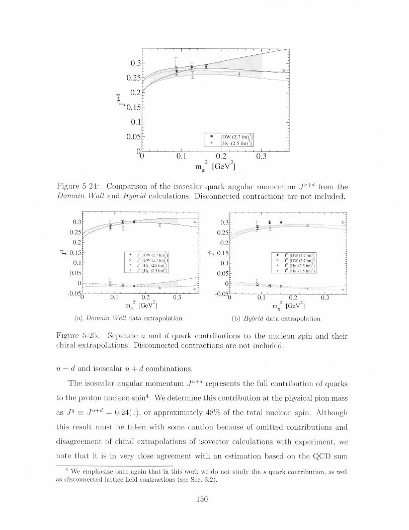
7+
0.2m 2 [GeV ]
Figure 5-24: Comparison of the isoscalar quark angular momentum ju+d from theDomain Wall and Hybrid calculations. Disconnected contractions are not included.
0.3 0.31-
0.25 ' 0.25--
0.2 0.2
0.15 . J DW (2.7 fim) 1 0.15 - J [DW (2.7 fm) ]
[DW (2.7fm ] fl J [DW (2.7 fm)0.1 J' [Hy (2.5 fm)] - J [Hy (2.5 fmi) |3 d 3
0.05 H 2.5 fm) 005 J Hy (2.5 fmi)
0 ~--------- - 07L
-0.0 r . . . . . I ' _0_0'-_ _ __._._._._ _
0 0.1 0.2 0.3 0 0.1 0.2 0.3m 2 [GeV 2] [GeV ]
(a) Domain Wall data extrapolation (b) Hybrid data extrapolation
Figure 5-25: Separate a and d quark contributions to the nucleon spill and theirchiral extrapolations. Disconnected contractions are not included.
u - d and isoscalar u + d combinations.
The isoscalar angular momentum Ju+d represents the full contribution of quarks
to the proton nucleon spin4 . We determine this contribution at the physical pion mass
as jq = Ju+d = 0.24(1), or approximately 48% of the total nucleon spin. Although
this result must be taken with some caution because of omitted contributions and
disagreement of chiral extrapolations of isovector calculations with experiment, we
note that it is in very close agreement with an estimation based on the QCD sum
4 We emphasize once again that in this work we do not study the s quark contribution, as wellas disconnected lattice field contractions (see Sec. 3.2).
150
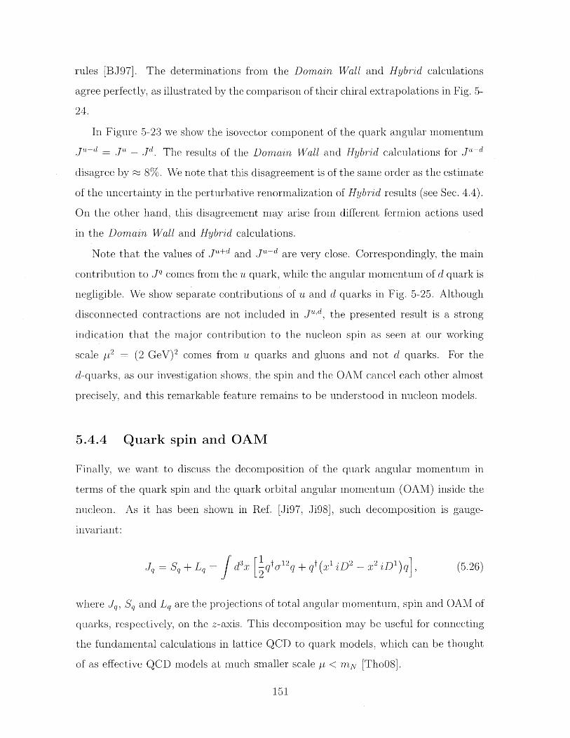
rules [BJ97]. The determinations from the Domain Wall and Hybrid calculations
agree perfectly, as illustrated by the comparison of their chiral extrapolations in Fig. 5-
24.
In Figure 5-23 we show the isovector component of the quark angular momentum
J"a - J"L - Jr'. The results of the Domain Wall and Hybrid calculations for Ju--d
disagree by 8%. We note that this disagreement is of the same order as the estimate
of the uncertainty in the perturbative renormalization of Hybrid results (see Sec. 4.4).
On the other hand, this disagreement may arise from different fermion actions used
in the Domain Wall and Hybrid calculations.
Note that the values of Ju+d and JU d are very close. Correspondingly, the main
contribution to Jq comes from the u quark, while the angular momentum of d quark is
negligible. We show separate contributions of u and d quarks in Fig. 5-25. Although
disconnected contractions are not included in J",d the presented result is a strong
indication that the major contribution to the nucleon spin as seen at our working
scale p 2 = (2 GeV)2 comes from u quarks and gluons and not d quarks. For the
d-quarks, as our investigation shows, the spin and the OAM cancel each other almost
precisely, and this remarkable feature remains to be understood in nucleon models.
5.4.4 Quark spin and OAM
Finally, we want to discuss the decomposition of the quark angular momentum in
terms of the quark spin and the quark orbital angular momentum (OAM) inside the
nucleon. As it has been shown in Ref. [Ji97, Ji98], such decomposition is gauge-
invariant:
Jq = S + L= dJ x [qtg12q + t (x1 iD 2 2 iDl)q], (5.26)
where Jq, S9 and Lq are the projections of total angular momentum, spin and OAM of
quarks, respectively, on the z-axis. This decomposition may be useful for connecting
the fundamental calculations in lattice QCD to quark models, which can be thought
of as effective QCD models at much smaller scale yt < mN [Tho08].
151
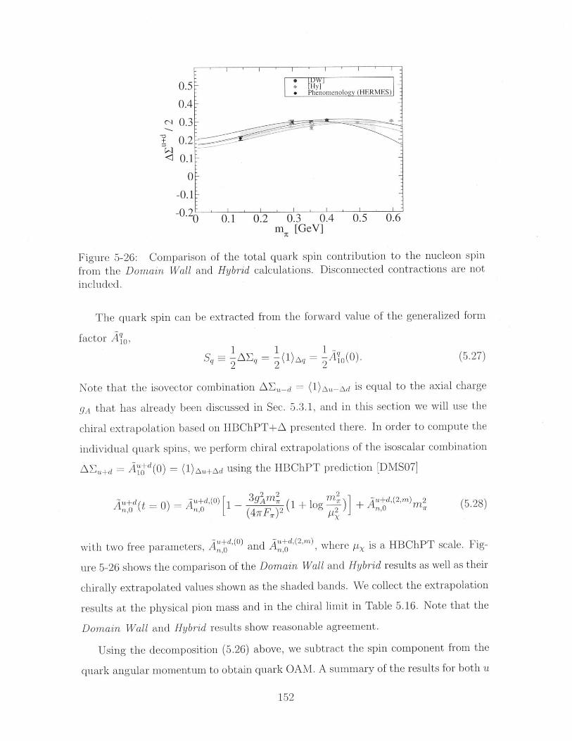
0.57Hy ePhenomenology (HERMES)
0.4--
0. -
<0. 1
0 -
-0.10.2o 0.1 0.2 0.3 0.4 0.5 0.6
m [GeV]
Figure 5-26: Comparison of the total quark spin contribution to the nucleon spin
from the Domain Wall and Hybrid calculations. Disconnected contractions are notincluded.
The quark spin can be extracted from the forward value of the generalized form
factor Aq0 ,1 1 1-
S - A = - -= A (0). (5.27)q 2 2 2
Note that the isovector combination AE-d = (I)Au-Ad is equal to the axial charge
gA that has already been discussed in Sec. 5.3.1, and in this section we will use the
chiral extrapolation based on HBChPT+A presented there. In order to compute the
individual quark spins, we perform chiral extrapolations of the isoscalar combination
AEu+A = A0() =(1)A+Ad using the HBChPT prediction [DMS07]
A"+(t =0) =Au+,(O) ]2(+o Au+d,( 2,m)m20) - AudO) I -gm (I+ og ir nO 7r (5.28)
nO L (47TF 7r )2 ( plo
with two free parameters, A'd() and Au'(2,m), where pX is a HBChPT scale. Fig-
ure 5-26 shows the comparison of the Domain Wall and Hybrid results as well as their
chirally extrapolated values shown as the shaded bands. We collect the extrapolation
results at the physical pion mass and in the chiral limit in Table 5.16. Note that the
Domain Wall and Hybrid results show reasonable agreement.
Using the decomposition (5.26) above, we subtract the spin component from the
quark angular momentum to obtain quark OAM. A summary of the results for both u
152
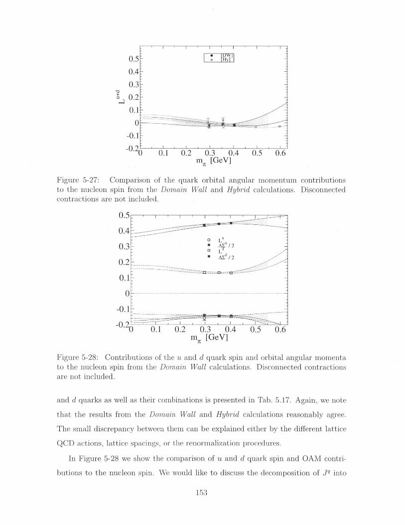
0.50.4
0.3
0.2
0.1
0
-0.1
-0.2 0.1 0.2 0.3 0.4m. [GeV]
Figure 5-27: Comparison of the quark orbital angular momentum contributionsto the nucleon spin from the Domain Wall and Hybrid calculations.contractions are not included.
0.5
0.4
0.3
0.2
0.1
0
-0.1
-0.20() 0.1 0.2 0.3 0.4mR [GeV]
0.5 0.6
Disconnected
Figure 5-28: Contributions of the u and d quark spin and orbital angular momentato the nucleon spin from the Domain Wall calculations. Disconnected contractionsare not included.
and d quarks as well as their combinations is presented in Tab. 5.17. Again, we note
that the results from the Domain Wall and Hybrid calculations reasonably agree.
The small discrepancy between them can be explained either by the different lattice
QCD actions, lattice spacings, or the renormalization procedures.
In Figure 5-28 we show the comparison of u and d quark spin and OAM contri-
butions to the nucleon spin. We would like to discuss the decomposition of jq into
153
.. I 1I. , ,
-.
I I IJ
0.5 0.6
o L"
A/2
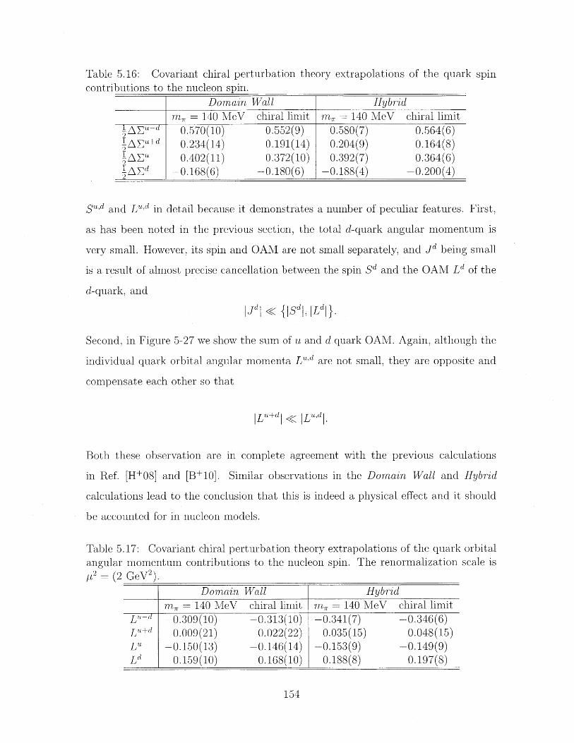
Table 5.16: Covariant chiral perturbation theory extrapolations of the quark spincontributions to the nucleon spin.
Domain Wall Hybridm, = 140 MeV chiral limit m, = 140 MeV chiral limit
1A E-d 0.570(10) 0.552(9) 0.580(7) 0.564(6)2AzE+d 0.234(14) 0.191(14) 0.204(9) 0.164(8)2~AE" 0.402(11) 0.372(10) 0.392(7) 0.364(6)lAzd -0.168(6) -0.180(6) -0.188(4) -0.200(4)
S"Ad and Lud in detail because it demonstrates a number of peculiar features. First,
as has been noted in the previous section, the total d-quark angular momentum is
very small. However, its spin and OAM are not small separately, and jd being small
is a result of almost precise cancellation between the spin Sd and the OAM Ld of the
d-quark, and
jd| < {Sd"| ILd|}.
Second, in Figure 5-27 we show the sum of u and d quark OAM. Again, although the
individual quark orbital angular momenta L'd are not small, they are opposite and
compensate each other so that
| Lu+I <|L"l.
Both these observation are in complete agreement with the previous calculations
in Ref. [H+08] and [B+10]. Similar observations in the Domain Wall and Hybrid
calculations lead to the conclusion that this is indeed a physical effect and it should
be accounted for in nucleon models.
Table 5.17: Covariant chiral perturbation theory extrapolations of the quark orbitalangular momentum contributions to the nucleon spin. The renormalization scale ispL2 = (2 GeV2 ).
Domain Wall Hybrid
m = 140 MeV chiral limit m, = 140 MeV chiral limit
LU-d -0.309(10) -0.313(10) -0.341(7) -0.346(6)Lut+d 0.009(21) 0.022(22) 0.035(15) 0.048(15)L" -0.150(13) -0.146(14) -0.153(9) -0.149(9)Ld 0.159(10) 0.168(10) 0.188(8) 0.197(8)
154
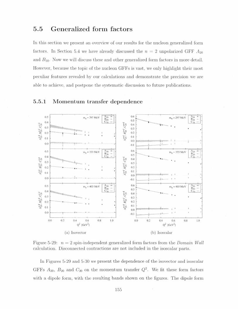
5.5 Generalized form factors
In this section we present an overview of our results for the nucleon generalized form
factors. In Section 5.4 we have already discussed the n = 2 unpolarized GFF A 2 0
and B 20 . Now we will discuss these and other generalized form factors in more detail.
However, because the topic of the nucleon GFFs is vast, we only highlight their most
peculiar features revealed by our calculations and demonstrate the precision we are
able to achieve, and postpone the systematic discussion to future publications.
5.5.1 Momentum transfer dependence
0.2 0.4 0.6
Q2 [GeV2
(a) Isovector
0.8 1.0
0.6in,-
0.5
0.4
0.3
0.2
0.1
0.0 p-0.1
0.6 m -3
0.5
0.4
0.3
0.2
0.1
0 .
-0 .1 .......I II
0.6 -m,, =
0.5
0.4
0.3
0.2
0.1
0.0
-0.1
0.0 0.2 0.4 0.6
Q2 [GeV2]
(b) Isoscalar
Figure 5-29: n = 2 spin-independent generalized form factors from the Domain Wallcalculation. Disconnected contractions are not included in the isoscalar parts.
In Figures 5-29 and 5-30 we present the dependence of the isovector and isoscalar
GFFs A20 , B 20 and C20 on the momentum transfer Q2. We fit these form factors
with a dipole form, with the resulting bands shown on the figures. The dipole form
155
in- 297 McV 20
C7
I -
- - 355 MeV A20B20CNI
-17m 403 MeV 20B20
C ..... ....
0.5
0.4
0.3
0.2
0.1
0.0
0.5
0.4
0.3
0.2
0.1
0.0
0.5
0.4
0.3
0.2
0.1
0.0
0 0.8 1.0.0
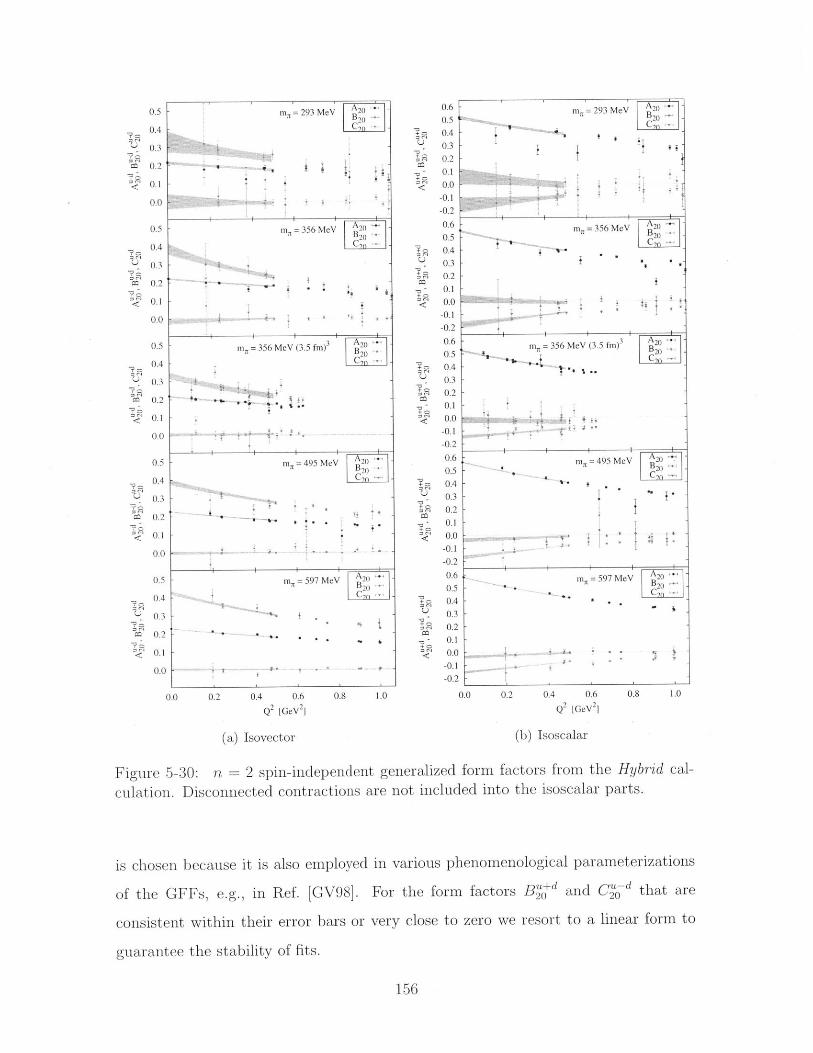
0.5
0.4
0.3
0.2
0.1
0.0
0.5
0.4
0.3
0.2
0.1
0.0
0.0 0.2 0.4 0.6 0.8 1.0
Q2 GeV2 1
(a) Isovector
Figure 5-30:
0.6 i,, 293 MeV 20
0.5 C20
0.4
0.30.20.10.0 K
-0.1-0.2
0.6 mit =356 MeV A20 -
0.5 B20
0.4 -
0.3 -0.20.10.0'. $
-0.1-0.2
in =36M 3 200.5 - m 356 MeV (3.5 fm) B20
0.4
0.30.20.10.0
-0.1 -
-0.2
0.6 mi =495 MeV 200.5 1 20
0.4 * * , Con
0.3-0.2-
0.10.0 t~0.1-0.2
0.6 m 5 97 MeV 200.5 -20.4
0.30.2
0.10.0 4
-0.1
-0.2
0.0 0.2 0.4 0.6 0.8 1.0
Q2 [GeV 2
(b) Isoscalar
n = 2 spin-independent generalized form factors from the Hybrid cal-
culation. Disconnected contractions are not included into the isoscalar parts.
is chosen because it is also employed in various phenomenological parameterizations
of the GFFs, e.g., in Ref. [GV98). For the form factors Be+d and C- d that are
consistent within their error bars or very close to zero we resort to a linear form to
guarantee the stability of fits.
156
Results of both the Domain Wall and Hybrid calculations demonstrate similar
trends for the magnitude of n = 2 unpolarized GFFs,
|Cje"| < |A'd- I< |B d
B ,+d < |Cugd| < |A u/d l.
The relative magnitude of the form factors is of interest because according to Eq. (1.21)
C2o(t) determines the dependence of the generalized moments H n=2(, t) and E n=2( t)
on the longitudinal momentum fraction . The (approximate) independence of the
n = 2 isovector generalized moments H =2 and En=2 may be a relevant constraint
for phenomenological analyses of future experimental data.
In addition, comparing isovector and isoscalar GFFs, we find qualitative agree-
ment with the large-Nc scaling rules [GPV01],
|A u-d|~ Ne <|A jd|~ N ,
|B20 ~0 NC> Bj|~N
Clod 3 N 7<jC~d 2N
|Cqu0-6 ~ Ne < |Cgu|d ~ 2|
The data for spin-dependent form factors has generally more stochastic variation.
In Figure 5-31 we show the Q2-dependence of the spin-dependent generalized form
factors A 2M and B20. There is no spin-dependent counterpart of C20 . We fit A 20 with a
dipole form and B 2 0 with a linear form in the entire available range 0 < Q2 < 1 GeV 2 .
We also present our observations how the Q2-dependence of the zero-skewness
generalized moment H"(( = 0, Q2) = A,,o changes with n. It is easy to see from
Eq. (1.18) that increasing n leads to amplifying the contribution of the quarks with
large longitudinal momentum fraction x to the H"( = 0, Q2) moment. On the other
hand, the 2D Fourier transform of the distribution H(x, = 0, -Q2) in the transverse
plane
H(x, b2) f T$e ib9 q-L H(x, = 0, t = -q) (5.29)
has a probability interpretation [BurOO] for a quark to be found at the transverse
157
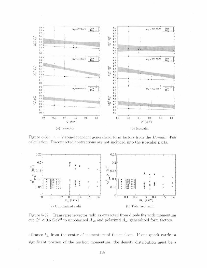
m = 297 MeV0.8B0.70.60.50.40.30.20.10.0
0.9 V 20(0.8 Cm = 355 MeV B,0.70.60.50.40.3 -0.2 - *0.10.0
mit =403 MeV 20070.60.5040.30.20.10.0
0.0 0.2 0.4 0.6 0.8 1.0
Q2 [GeV
21
(a) Isovector
0.9 m =297 MeV
0.70.60.50.40.30.20.10.0
m 355 MeV A,)()0.8 B.-a)r0.70.60.50.40.30.2 -0.10.0
I1 i
0.9m: = 403 MeV 200.8 itB,
0.70.60.50.40.3 -
0.20.1 ...
0.0
0.0 0.2 0.4 0.6 0.8 1.0
Q2 [GeV2
(b) Isoscalar
n = 2 spin-dependent generalized form factors from the Domain Wallcalculation. Disconnected contractions are not included into the isoscalar parts.
I . II I I I
N
~
*DW n =2ADW n= 3
S Hy] n=1
- Hy] n-
0.1 0.2 0.3 0.4m [GeV]
(a) Unpolarized radii
0.5 0.6
0.25 1
0.2-
0.15 -A
. 0.1
0.05- .I
.
DW n 2'DW n 3Hy] n-I IHy] n-2H n n
"0 0.1 0.2 0.3 0.4m, [GeV]
(b) Polarized radii
Figure 5-32: Transverse isovector radii as extracted from dipole fits with momentumcut Q2 < 0.5 GeV 2 to unpolarized Ao and polarized Ao generalized form factors.
distance b_ from the center of momentum of the nucleon. If one quark carries a
significant portion of the nucleon momentum, the density distribution must be a
158
Figure 5-31:
0.25r-
0.2-
0.15-A
1-0. 0. 1
0.05
0.5 0.6
.
5
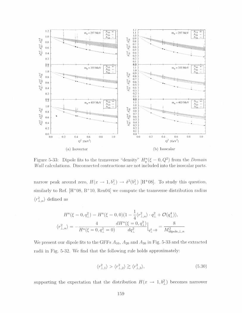
n 297 MeV
m 355 MeV
m7 =403 MeV
A
0.2 0.4 0.6 0.8 1.0
Q2 [GeV 2]
100.90.80.70.60.50.40.30.20.1D.01.11.00.90.80.70.60.50.40.30.20.10.51.11.00.90.80.70.60.50.40.30.20.10.0
0
(a) Isovector
0.2 0.4 . 0.6 0.8 1.0
Q2 1GeV
2]
(b) Isoscalar
Dipole fits to the transverse "density" Hq"( = 0, Q2) from the DomainWall calculations. Disconnected contractions are not included into the isoscalar parts.
narrow peak around zero, H(x -+ 1, bI) -> 62 (bI) [H+08]. To study this question,
similarly to Ref. [H+08, B+10, RenO4] we compute the transverse distribution radius
Kri,) defined as
H"'((=0, q) H(= 0, 0)(11-(ri ,) qj + O(q)),
4 dH"(=0,qg) 8" Hl"( = 0,qi = 0) dqi 2 41=20 M2so
We present our dipole fits to the GFFs A10, A20 and A30 in Fig. 5-33 and the extracted
radii in Fig. 5-32. We find that the following rule holds approximately:
(rI2) > (rI,) > (rI,), (5.30)
supporting the expectation that the distribution H(x -> 1, bI) becomes narrower
159
.0
Mr 297 MeV 10A2 01A.
m11 7 355 MeV 10
Aj.
- -
m 403 MeV toA20
- A.
0.6
0.4 [0.2
0.0 -0.0
Figure 5-33:
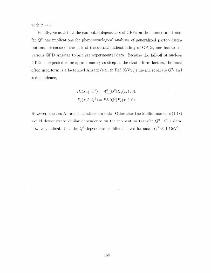
with x -> 1.
Finally, we note that the computed dependence of GFFs on the momentum trans-
fer Q2 has implications for phenomenological analyses of generalized parton distri-
butions. Because of the lack of theoretical understanding of GPDs, one has to use
various GPD Ansdtze to analyze experimental data. Because the fall-off of nucleon
GPDs is expected to be approximately as steep as the elastic form factors, the most
often used form is a factorized Ansatz (e.g., in Ref. [GV98]) having separate Q2- and
x-dependence,
Hq(x, , Q2 ) = Aq0 (Q2)Hq(x, , 0),
Eq(x, 1, Q2) = Bl0 (Q2 )Eq(x, , 0).
However, such an Ansatz contradicts our data. Otherwise, the Mellin moments (1.18)
would demonstrate similar dependence on the momentum transfer Q2. Our data,
however, indicate that the Q2-dependence is different even for small Q2 < 1 GeV 2.
160
Chapter 6
Summary
In this work we have performed high-statistics, high-precision calculations of nucleon
structure observables in the framework of lattice QCD. This is the first calculation
of nucleon structure observables using QCD on a lattice with chiral quarks and pion
masses as low as ~~ 300 MeV. We have carefully studied the systematic effects that
can arise in computing nucleon matrix elements of quark operators, and applied
optimization techniques to eliminate them as much as possible. As a result, we
are able to reduce the Euclidean time distance in the nucleon correlation functions,
which would otherwise be necessary to prevent systematic bias, and thus to improve
considerably the signal-to-noise ratio in our calculations.
We perform our calculations using three different discretizations of the QCD action
with Domain Wall (chiral sea and valence quarks), Hybrid (non-chiral sea and chiral
valence quarks), and Wilson-Clover, (non-chiral valence and sea quarks), or BMW,
fermions. The motivation to use the three different actions is twofold. First, a
direct comparison of the results allows us to estimate systematic effects arising from
simulating QCD on a lattice and assess the level at which different discretizations
affect the observables we calculate. Second, Wilson-Clover action is significantly
cheaper and allows us to obtain results at lighter pion masses at the expense of chiral
symmetry breaking.
Because the differences in fundamental theory can lead to differences in effective
theory parameters, one may not perform simultaneous chiral extrapolations of these
161
calculations Nevertheless, the results of both calculations agree reasonably well for
all the observables we compute, and this fact reassures us that our methodology is
correct and systematic effects are under control. In addition, since the lattice spacing
is different in these two cases, the agreement of our results indicates that discretization
errors in our calculations are small.
The results we report include the nucleon vector and axial form factors, the gen-
eralized form factors, the quark spin and angular momentum contributions to the
nucleon spin. We observe that the dependence of the nucleon form factors on the
momentum transfer is qualitatively similar to phenomenology and experiments. For
example, we successfully use a dipole form to model the isovector Sachs electric form
factor. However, the size parameters we extract from our calculations, such as the
r.m.s. radii of charge, magnetization, and axial distributions in the nucleon, are
considerably smaller than experimental values. This is not surprising since we are
working with pion masses at least twice as heavy as the physical pion mass, and the
nucleon is known to be surrounded by a virtual pion cloud, which contributes to the
nucleon structure probed by experiments and our calculations.
The most precise results of our calculation, the nucleon vector form factors, pro-
vide a unique opportunity to test the predictions of chiral perturbation theory. Pre-
viously, either heavy pion masses or large stochastic variation prohibited testing pre-
dictions of ChPT, as well as extrapolating the results of lattice calculations to the
physical pion mass reliably. Our new data indicate, however, that neither O(Es)
HBChPT+A (also known as small-scale expansion, or SSE) nor 0(p 4 ) CBChPT ef-
fective theories can accommodate both our new lattice data and experimental results
simultaneously. We draw the conclusion that these chiral perturbation theory calcu-
lations of Dirac and Pauli radii, at this specific order of approximation, cannot be
valid in the range of pion masses above m, ;> 300 MeV.
One part of our results is renormalized non-perturbatively, and the other part is
renormalized using perturbative lattice renormalization factors. We compare the per-
turbative renormalization factors to non-perturbative calculations, and estimate their
difference as ~ 10%. We thus establish a remarkable result that lattice perturbative
162

renormalization may introduce a systematic bias of order of 10%. This conclusion is
an important enhancement of the previous studies of the nucleon structure reported
in Refs. [H+08, B+10].
Finally, as has been discussed before, our calculations of nucleon structure are
not complete yet. We do not compute the s-quark contribution to the nucleon struc-
ture, and omit disconnected diagrams contributing to nucleon isoscalar observables.
However, the methods we developed to control the lattice systematic effects in nu-
cleon matrix elements arising from excited state contributions will be necessary for
reliable calculations of these quantities. Therefore, in this work we have laid essential
foundation for studies of full quark contributions to nucleon structure in lattice QCD.
163
164
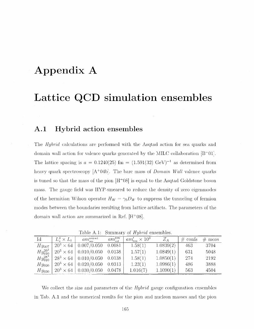
Appendix A
Lattice QCD simulation ensembles
A.1 Hybrid action ensembles
The Hybrid calculations are performed with the Asqtad action for sea quarks and
domain wall action for valence quarks generated by the MILC collaboration [B+01].
The lattice spacing is a = 0.1240(25) fm = (1.591(32) GeV)-' as determined from
heavy quark spectroscopy [A+04b]. The bare mass of Domain Wall valence quarks
is tuned so that the mass of the pion [H+08] is equal to the Asqtad Goldstone boson
mass. The gauge field was HYP-smeared to reduce the density of zero eigenmodes
of the hermitian Wilson operator Hw - 35Dw to suppress the tunneling of fermion
modes between the boundaries resulting from lattice artifacts. The parameters of the
domain wall action are summarized in Ref. [H+08].
Table A.1: Summary of Hybrid ensembles.
Id L3 x Lt am " amDW am/ X 103 ZA # confs # measHy007 203 x 64 0.007/0.050 0.0081 1.58(1) 1.0839(2) 463 3704
Hy20 203 x 64 0.010/0.050 0.0138 1.57(1) 1.0849(1) 631 5048Hy2, 283 x 64 0.010/0.050 0.0138 1.58(1) 1.0850(1) 274 2192Hyo2o 203 x 64 0.020/0.050 0.0313 1.23(1) 1.0986(1) 486 3888Hyo3o 203 x 64 0.030/0.050 0.0478 1.016(7) 1.1090(1) 563 4504
We collect the size and parameters of the Hybrid gauge configuration ensembles
in Tab. A.1 and the numerical results for the pion and nucleon masses and the pion
165
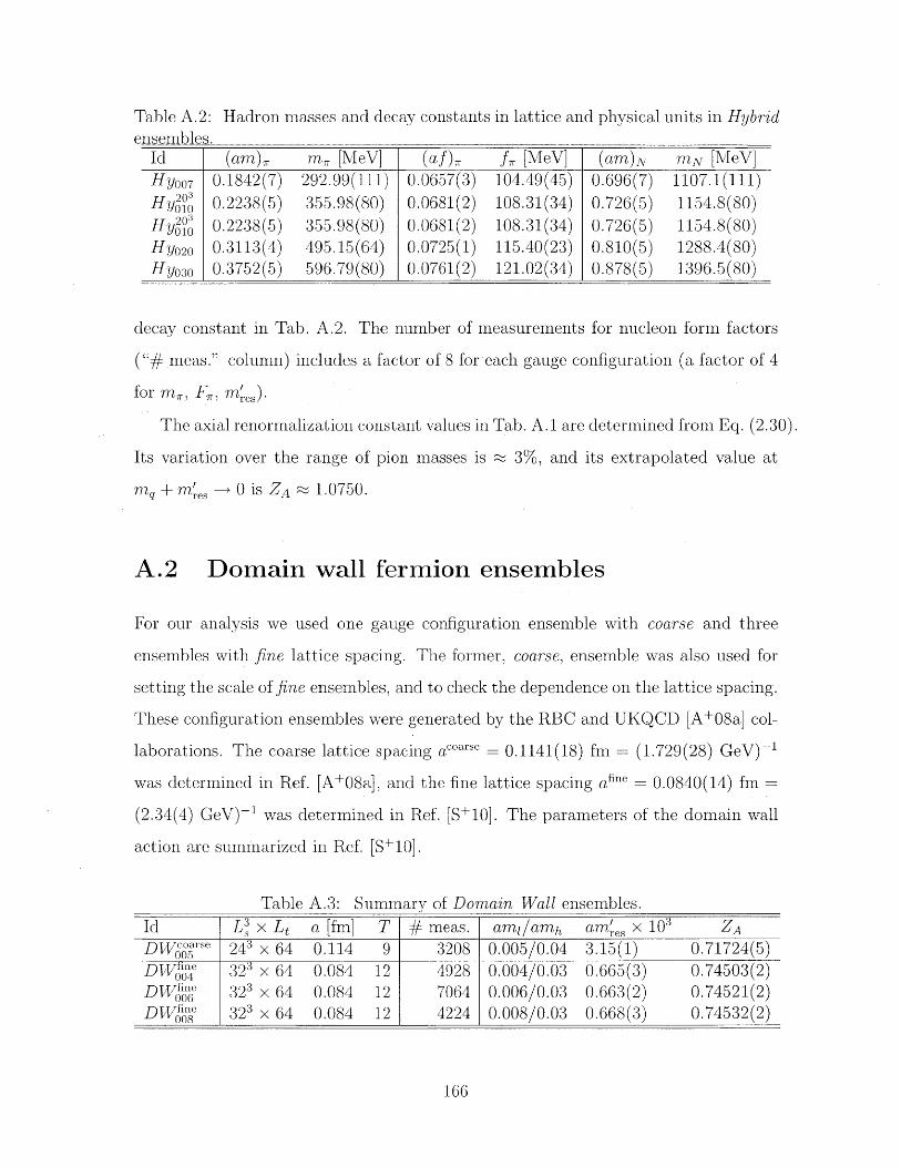
Table A.2: Hadron masses and decay constants in lattice and physical units in Hybridensembles.
Id (am), m, [MeV] (af), f, [MeV] (am)N mN [MeV]Hyoo7 0.1842(7) 292.99(111) 0.0657(3) 104.49(45) 0.696(7) 1107.1(111)Hy 0.2238(5) 355.98(80) 0.0681(2) 108.31(34) 0.726(5) 1154.8(80)Hyoj 0.2238(5) 355.98(80) 0.0681(2) 108.31(34) 0.726(5) 1154.8(80)Hy 0 20 0.3113(4) 495.15(64) 0.0725(1) 115.40(23) 0.810(5) 1288.4(80)
Hy 03 0.3752(5) 596.79(80) 0.0761(2) 121.02(34) 0.878(5) 1396.5(80)
decay constant in Tab. A.2. The number of measurements for nucleon form factors
("# meas." column) includes a factor of 8 for each gauge configuration (a factor of 4
for m,, F,, m'res).
The axial renormalization constant values in Tab. A.1 are determined from Eq. (2.30).
Its variation over the range of pion masses is a 3%, and its extrapolated value at
m +m -* 0 is ZA ~1.0750.
A.2 Domain wall fermion ensembles
For our analysis we used one gauge configuration ensemble with coarse and three
ensembles with fine lattice spacing. The former, coarse, ensemble was also used for
setting the scale of fine ensembles, and to check the dependence on the lattice spacing.
These configuration ensembles were generated by the RBC and UKQCD [A+08a] col-
laborations. The coarse lattice spacing acoarse = 0.1141(18) fm = (1.729(28) GeV)-'
was determined in Ref. [A+08a], and the fine lattice spacing a fine = 0.0840(14) fm =
(2.34(4) GeV)-1 was determined in Ref. [S+10]. The parameters of the domain wall
action are summarized in Ref. [S+10].
Table A.3: Summary of Domain Wall ensembles.
Id L 3 x Lt a [fm] T # meas. ami/amh a res 3 ZADWogrse 243 x 64 0.114 9 3208 0.005/0.04 3.15(1) 0.71724(5)DWfon~e 323 x 64 0.084 12 4928 0.004/0.03 0.665(3) 0.74503(2)DWone"; 323 x 64 0.084 12 7064 0.006/0.03 0.663(2) 0.74521(2)DVWoin" 323 x 64 0.084 12 4224 0.008/0.03 0.668(3) 0.74532(2)
166
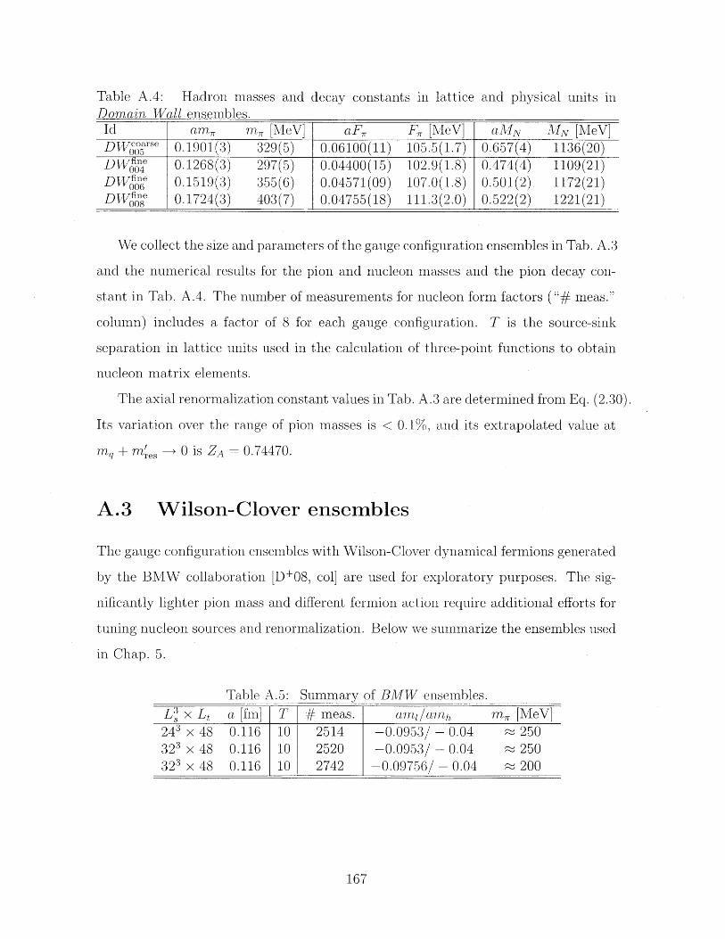
Table A.4: Hadron masses and decay constants in lattice and physical units inDomain Wall ensembles.
Id am, mr (MeV] aF, FT [MeV] aMN MN [MeV]DVesarse 0.1901(3) 329(5) 0.06100(11) 105.5(1.7) 0.657(4) 1136(20)DWne 0.1268(3) 297(5) 0.04400(15) 102.9(1.8) 0.474(4) 1109(21)DWneg 0.1519(3) 355(6) 0.04571(09) 107.0(1.8) 0.501(2) 1172(21)DW 5 s* 0.1724(3) 403(7) 0.04755(18) 111.3(2.0) 0.522(2) 1221(21)
We collect the size and parameters of the gauge configuration ensembles in Tab. A.3
and the numerical results for the pion and nucleon masses and the pion decay con-
stant in Tab. A.4. The number of measurements for nucleon form factors ("# meas."
column) includes a factor of 8 for each gauge configuration. T is the source-sink
separation in lattice units used in the calculation of three-point functions to obtain
nucleon matrix elements.
The axial renormalization constant values in Tab. A.3 are determined from Eq. (2.30).
Its variation over the range of pion masses is < 0.1%, and its extrapolated value at
mq + ms -> 0 is ZA = 0.74470.
A.3 Wilson-Clover ensembles
The gauge configuration ensembles with Wilson-Clover dynamical fermions generated
by the BMW collaboration [D+08, col] are used for exploratory purposes. The sig-
nificantly lighter pion mass and different fermion action require additional efforts for
tuning nucleon sources and renormalization. Below we summarize the ensembles used
in Chap. 5.
Table A.5: Summary of BMW ensembles.x Lt a [fn] T # meas. ami/amh m., MeV]
243 x 48 0.116 10 2514 -0.0953/ - 0.04 250323 x 48 0.116 10 2520 -0.0953/ - 0.04 250323 x 48 0.116 10 2742 -0.09756/ - 0.04 200
167

168
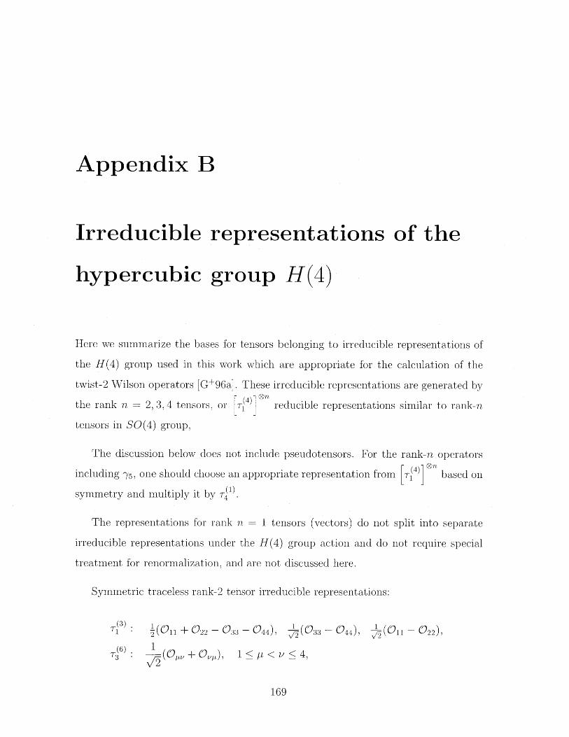
Appendix B
Irreducible representations of the
hypercubic group H(4)
Here we summarize the bases for tensors belonging to irreducible representations of
the H(4) group used in this work which are appropriate for the calculation of the
twist-2 Wilson operators [G+96a]. These irreducible representations are generated by
the rank n = 2, 3, 4 tensors, or r 4)] reducible representations similar to rank-n
tensors in SO(4) group,
The discussion below does not include pseudotensors. For the rank-n operators
including '7, one should choose an appropriate representation from [(4)] based on(1)i
symmetry and multiply it by r.
The representations for rank n = 1 tensors (vectors) do not split into separate
irreducible representations under the H(4) group action and do not require special
treatment for renormalization, and are not discussed here.
Symmetric traceless rank-2 tensor irreducible representations:
(11 + 022 - 033- 044), -(033 - 044), (On -Q22),
(6) 1 +1 (0y < 473 - v2 -v+< 4
169
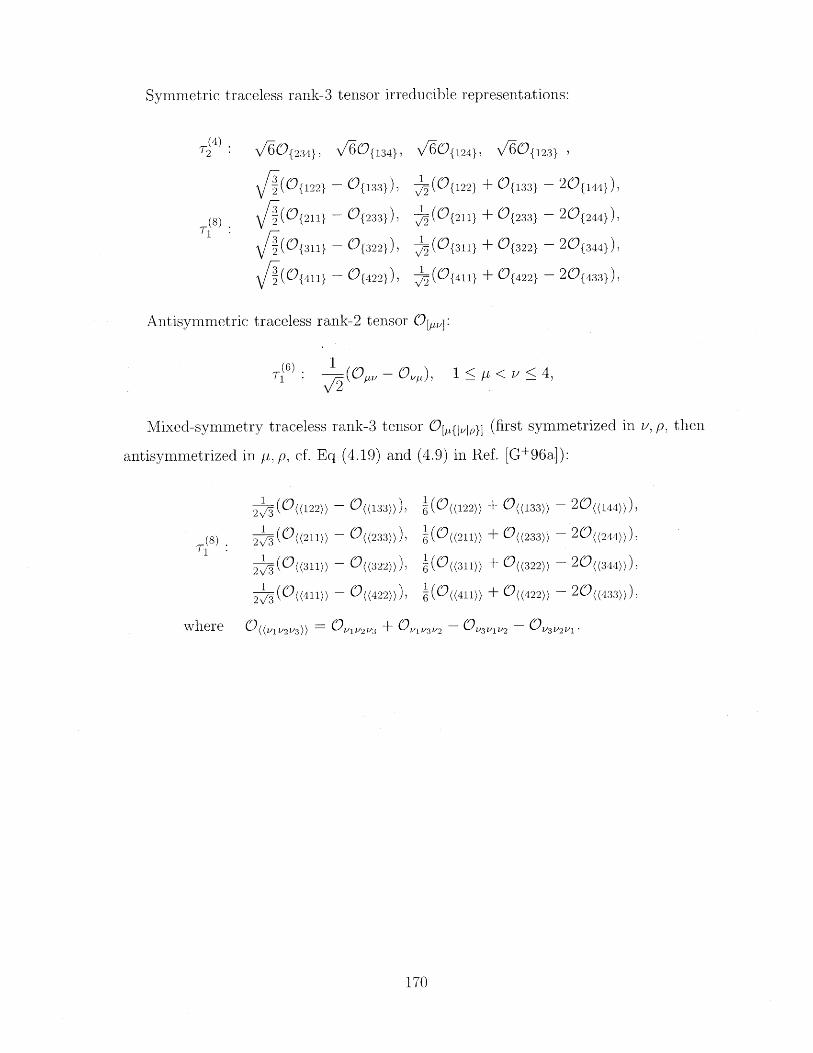
Symmetric traceless rank-3 tensor irreducible representations:
(4)60{234} {60f134}, 60{124}, {60123}
{(Of122} - O{133})
(8) : 2jQ{211} - O{233})
1i -{311} {- O322}),
V(Q{411} - O{422})
2(0{122} + O{133} - 20{144}),
(211 + O{233}
{(0311 + 0{322}
- 20{244}),
- 20{344}))
1411}+ 422 -- 20{433}),
Antisymmetric traceless rank-2 tensor 0
(6) 1 0 -v - LPT 2
Mixed-symmetry traceless rank-3 tensor 0 ,f{I"pj} (first symmetrized in v, p, then
antisymmetrized in y, p, cf. Eq (4.19) and (4.9) in Ref. [G+96a]):
13((122)) O((133))) 1(0((122)) + ((133)) - 20((144))),
1 (G((211)) - O((233))),
13(0((311)) - ((322))>
1 ( (411)) -- ((422))),
6(C((211)) + O((233)) - 20((244))),
6(0((311)) + Q((322)) - 20((344))),
6(O((411)) + O((422)) - 20((433))),
where ( =V23) O-1V 2v 3 + 021V3Vv2 OsV3 1V 2 - OV3V21
170
(8)
I < ti < v < 4,
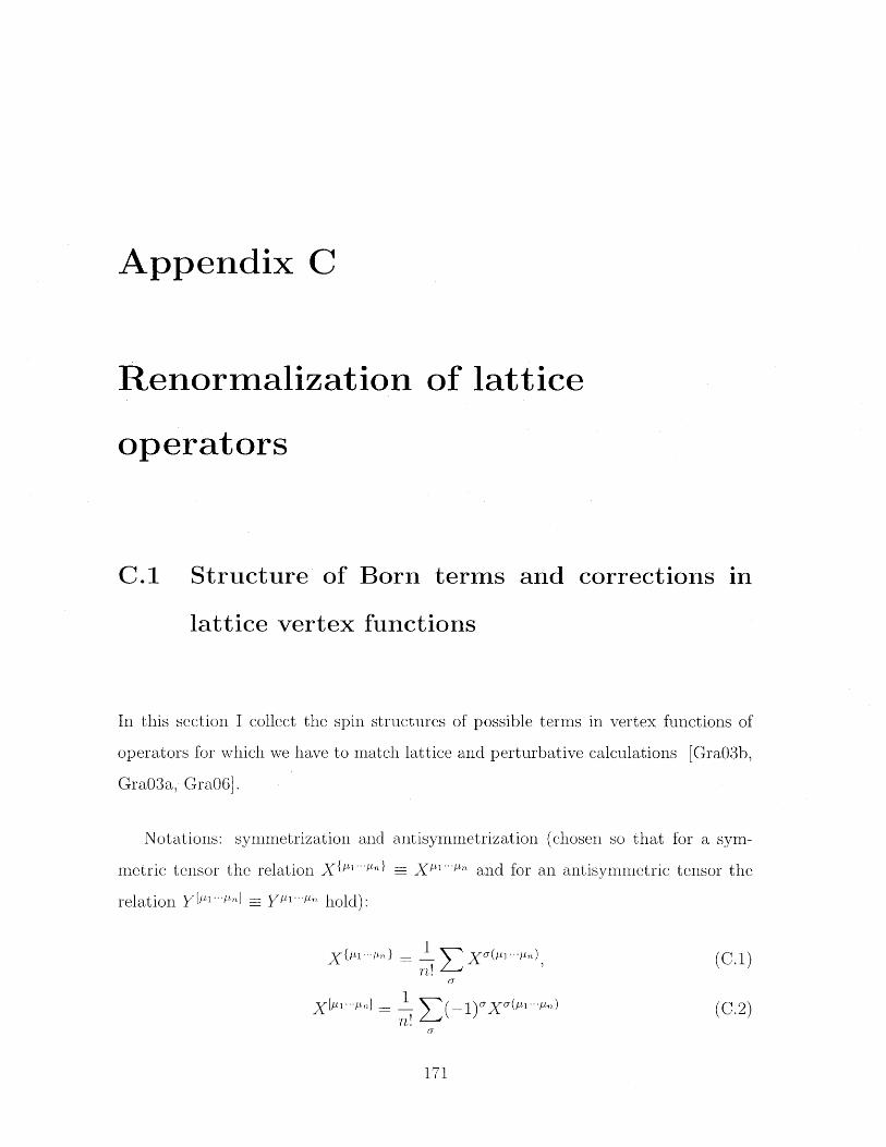
Appendix C
Renormalization of lattice
operators
C.1 Structure of Born terms and corrections
lattice vertex functions
In this section I collect the spin structures of possible terms in vertex functions of
operators for which we have to match lattice and perturbative calculations [Gra03b,
Gra03a, Gra06].
Notations: symmetrization and antisymmetrization (chosen so that for a sym-
metric tensor the relation Xf{1 l X1"'" and for an antisymmetric tensor the
relation Y1"..1-] = Y1./n hold):
1n!
1
a
0~
(C.1)
(C.2)
171
in
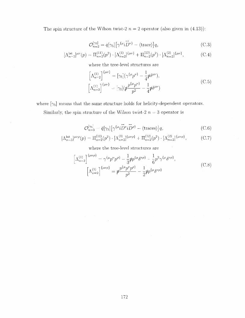
The spin structure of the Wilson twist-2 n = 2 operator (also given in (4.13)):
n=2 [ q[{75] [7Y}iD" - (trace)] q, (C.3)
[A 2a' (p) 2(I)(P2) - [AI)21 P"I + rl(12)(P2) - [A( 2 )]2fv) (CA)
where the tree-level structures are
L21 [7"} - p 1 06[t ) (C 5)
where [Y51 means that the same structure holds for helicity-dependent operators.
Similarly, the spin structure of the Wilson twist-2 n = 3 operator is
-3 75][7{"iD"iDP - (traces)]q, (C.6)
[A> 3 ]a (p) = H()(2) - [A) 2]L""P + Il( 1 2)(P2) . [A (2)] 2"WP" (C.7)
where the tree-level structures are
A(' 7{tW'Pl f vpp{ )P} !2h{LL6NIP}
) 3 6(C.8)
A 2 -- p2P - 2I '
172
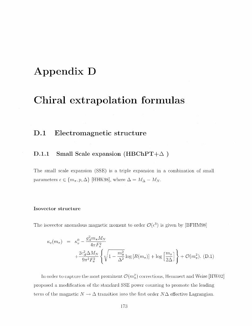
Appendix D
Chiral extrapolation formulas
D.1 Electromagnetic structure
D.1.1 Small Scale expansion (HBChPT+A)
The small scale expansion (SSE) is a triple expansion in a combination of small
parameters E E {m, p, A} [HHK98], where A = JA - MN.
Isovector structure
The isovector anomalous magnetic moment to order 0(E3) is given by [BFHM98)
gmMN-vm) = x 47rF3
+ 2cA N 1 log [R(m)] + log .+ (M 7) (D.1)
In order to capture the most prominent O(m2) corrections, Hennert and Weise [HW02]
proposed a modification of the standard SSE power counting to promote the leading
term of the magnetic N -+ A transition into the first order NA effective Lagrangian.
173
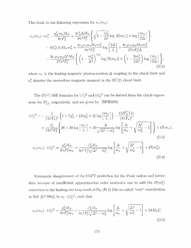
This leads to the following expression for r, (m,):
o 9i mMJrN 2cAMN 147F2 97r 2F LV8 r ~ 4CACVgA-A/I~VM2
- 8E (A)MNm2 + 7cvAN
1 7 972F,2
8cAcvgA A 2MN27-r2F
2)3/2
A2 f)l
(1I
log [R(rn,)1 + log [~rF2A2A
log RA] +
Og [R(mn,)] +
4CACV9AMNm r277FlA
3m022A2 f)
log2A
(D.2)
where cv is the leading magnetic photon-nucleon-A coupling in the chiral limit and
K0 denotes the anomalous magnetic moment in the SU(2) chiral limit.
The 0( 3 ) SSE formulas for (r,) 2 and (r) 2 can be derived from the chiral expres-
sions for F 2, respectively, and are given by [BFHM98]
1(4-rF1,) 2
2
+ CA54r 2F2
+ 7gA + (10g + 2)Alog [7}
LA]* + 30 logA 2 -_M2
+ c AN log9 72 F ? /2 - M,2
12B () (A)(47F,)2
A A2- + 1m m7 I
(D.3)
+ - I + O(MO.
(D.4)
Systematic disagreement of the ChPT prediction for the Pauli radius and lattice
data because of insufficient approximation order motivates one to add the O(m,)
correction to the leading one-loop result of Eq. (D.4) (the so-called "core" contribution
in Ref. [G+05b]) to s' - (r) 2 , such that
gAMN
8irFjm~ +
CAJNF A - log
92F2 /-2 - m2
[A A2
- + 1 + 24MN-
(D.5)
174
riv)2
26 + 30 log
gA MN
87rF m,KV (m,) - (r")2
-
+ O(m) ,
V (m)-(r)2 -
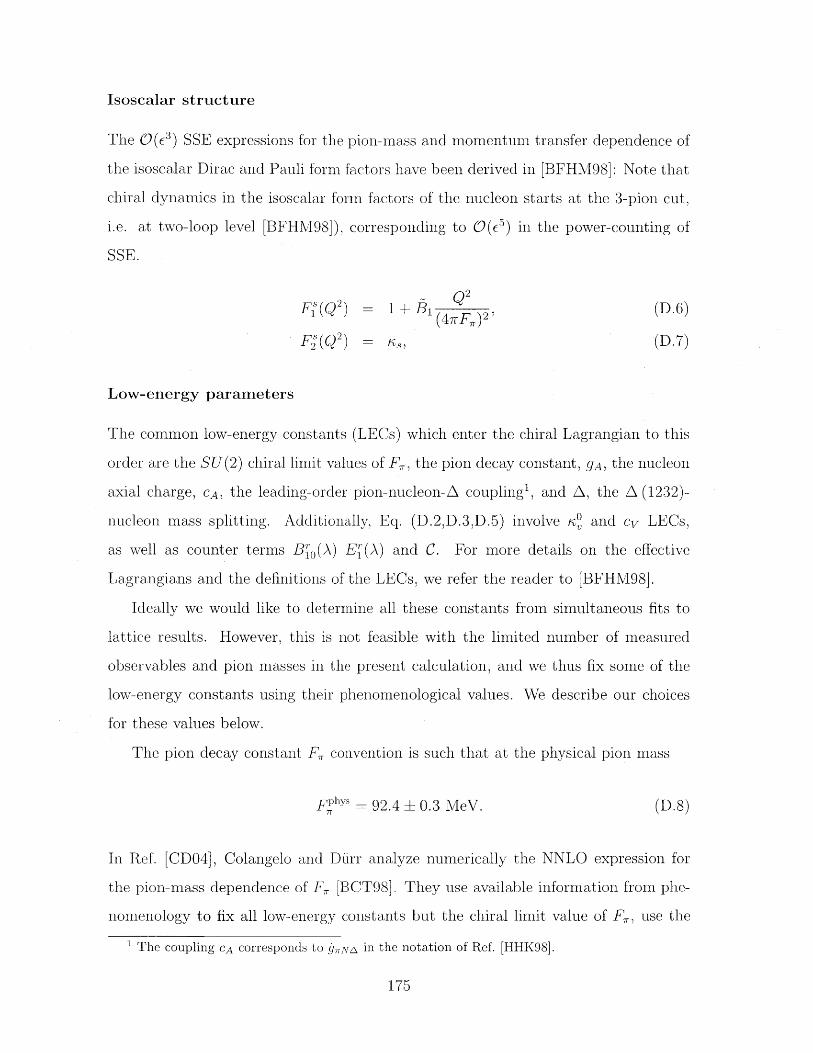
Isoscalar structure
The 0(Es) SSE expressions for the pion-mass and momentum transfer dependence of
the isoscalar Dirac and Pauli form factors have been derived in [BFHM98]: Note that
chiral dynamics in the isoscalar form factors of the nucleon starts at the 3-pion cut,
i.e. at two-loop level [BFHM98]), corresponding to 0(c5) in the power-counting of
SSE.
Fi (Q2 ) = + 51 2, (D.6)
Fj(Q2 ) = 2, (D.7)
Low-energy parameters
The common low-energy constants (LECs) which enter the chiral Lagrangian to this
order are the SU(2) chiral limit values of F., the pion decay constant, gA, the nucleon
axial charge, CA, the leading-order pion-nucleon-A coupling1 , and A, the A (1232)-
nucleon mass splitting. Additionally, Eq. (D.2,D.3,D.5) involve KO and cv LECs,
as well as counter terms Bl(,(A) E[(A) and C. For more details on the effective
Lagrangians and the definitions of the LECs, we refer the reader to [BFHM98].
Ideally we would like to determine all these constants from simultaneous fits to
lattice results. However, this is not feasible with the limited number of measured
observables and pion masses in the present calculation, and we thus fix some of the
low-energy constants using their phenomenological values. We describe our choices
for these values below.
The pion decay constant F, convention is such that at the physical pion mass
F hys : 92.4 ± 0.3 MeV. (D.8)
In Ref. [CD04], Colangelo and Diirr analyze numerically the NNLO expression for
the pion-mass dependence of F, [BCT98]. They use available information from phe-
nomenology to fix all low-energy constants but the chiral limit value of F,, use the
The coupling CA corresponds to y,1rA in the notation of Ref. [HHK98].
175
physical value (D.8) and obtain
F', chiral limit = (86.2 ± 0.5) MeV. (D.9)
In the absence of reliable chiral extrapolations of both nucleon and A (1232)
masses (see the discussion in Ref. [WL+09]) 2, we identify the A-nucleon mass split-
ting in the chiral limit with its value at the physical m, . The position of the A (1232)
resonance pole in the total center-of-mass energy plane has been determined from
magnetic dipole and electric quadrupole amplitudes of pion photoproduction. Ac-
cording to the Particle Data Group average [A+08b], the A-pole position leads to
MA = (1210 + 1) MeV and FA = (100 ± 2) MeV. If one instead defines the A (1232)
mass and width by looking at the 900 rN phase shift in the spin-3/2 isospin-3/2
channel, the PDG averages give MA = (1232 ± 1) MeV and FA = (118 ± 2) MeV.
With MN = 939 MeV, one obtains, respectively,
A = (271 ± 1) MeV, (D.10)
or
A = (293 + 1) MeV. (D.11)
The A (1232) decays strongly to a nucleon and a pion with almost 100% branching
fraction. From the PDG values of masses and widths [A+08b] and from
2
FA-N,= CA (E 2 - m 2 )3 / 2 (MA + MN - E7,), (D.12)12r F2 MA
whereM2 - MN2 + M2
E7, - 2M (D.13)
2 For an analysis of the quark-mass dependence of nucleon and delta masses in the covariant SSEat order c we refer to [BHM05].
176
one obtains, respectively 3,
CAJ = 1.50 ... 1.55 if F = (100 ± 2) MeV and A = (271 ± 1) MeV(D.17)
CA = 1.43. .. 1.47 if F = (118 ± 2) 1\eV and A = (293 ± 1) MeV(D.18)
Chiral extrapolations of different sets of lattice results [HPW03, E+06b, PMHW07,
AK+06] based on SSE at leading-one-loop accuracy lead to a chiral limit value for gA
of about 1.2. From the relativistic tree-level analysis of the process of pion photopro-
duction at threshold -yp - r0p, one obtains [DMW91, HHK97] (for CA =1.5)
cv ( 2.5 ± 0.4) GeV- . (D.19)
D.1.2 Covariant Baryon ChPT (CBChPT)
In this section we collect the nucleon structure results obtained in the formulation
of SU(2) chiral effective field theory in the baryon sector, without explicit A (1232)
degrees of freedom: covariant BChPT as introduced in Ref. [GSS88] with a modi-
fied version of infrared regularization (IR-scheme). For details about the formalism
and differences from the standard infrared regularization introduced by Becher and
Leutwyler [BL99], we refer the reader to Refs. [DGH08, Gai07, GH].
3 Calculating the strong decay width of A (1232) to leading order in (nonrelativistic) SSE kine-matics, one obtains
FAN rr A - M2)3/2. (D.14)
We note that this expression corresponds to the leading term in a 1/MN expansion of the resultgiven in Eq. (D.12), which utilizes the full covariant kinematics. Using the ranges of masses anddecay widths mentioned above, this expression yields the lower values
cAl = 1.11 .. .1.14 if F = (100 ± 2) MeV and A = (271 ± 1) MeV; (D.15)
|cAI = 1.04 ... 1.07 if F = (118 ± 2) MeV and A = (293 ± 1) MeV. (D.16)
Furthermore, SU(4) spin-flavor quark symmetry gives cA = 3 gA/(2 2) = 1.34.
177
Isovector structure
The expressions for the m, dependence of the mean squared isovector Dirac and Pauli
radii and the isovector anomalous magnetic moment have been derived in [Gai07] up
to order p4 i.e. at the next-to-leading one-loop accuracy and are collected below4.
For the isovector mean squared Dirac radius, the expression is given as
()2 = Bc1 + [(rv)2]( 3 ) + [(rv)2](4) + O(m), (D.20)
where
Bc1 = -12dr(A),
r 7gqM 4 + 2(5g2 + 1)M4 log + M - 15gimnM 2167r2FAM4 167 A
+ g2m 2 (15m 2 - 44M 2 ) log
2
+ g[m" 15m 4 - 74m2M 2 + 70M 4] arccos167r2F2M 4 -4M2 -m2 7 2M
(rv)2] _ 32 - 3MJ)arccos m167 2F 2 M 4M 2 - M2 2Mo
+ 4M - m2 MO2 + (M m ) log .]
The terms contributing up to and including 0(pi) are denoted by the superscript
(i). Without any loss of generality, the regularization scale A is set equal to MO, the
nucleon mass in the chiral limit. The low-energy constants d6 and c6 appear, respec-
tively, in the third- and second-order rN effective Lagrangian. The mass function M
must be identified with M0 if one truncates the previous expression at O(p3), whereas
4 In Ref. [Gai07] the form factor slopes pv and pv are used, which are related to our notation forry and r' by p' = 1(r ) 2 and p' = - (r,)2.
178
at order p4 , according to Ref. [Gai07), A should be replaced by [DGHO8]
AN (mr ) =-Ao3g 2m,3
4cim2 + 3 A7r327r2F 4 -
0I 0
12872 I 2 +
4 3Cig 2M 6+ 4e(A)m4 - Ag 7r log
7 8r 2F7 M2
4 (A11
i)
where 5
Bc2 = 24Moe74 (A),
2 m44 + "7_ + 4c1 3
M0 MA/s
- 8c1 + c2 + 4c3)
)arccos
log
(D.21)
where ci, c2 and c3 are second-order low-energy constants and e(A) denotes an effec-
tive coupling consisting of a combination of fourth order low-energy constants. In our
current analysis, we always include terms up to O(p'), hence M in all the BChPT
expressions presented here should be identified with MN(mr).
The pion-mass dependence of the isovector Pauli radius is given by
_ giMo167r2F2M5(m2 - 4M 2)
124M 6
+ 6(3m6 - 22M12m + 44M 4m -
2f -Al0o
87r2F2M 5m, (4jV2
216M 6m2 + 16MA8
+ 105m2M 4 - 18mn4M 2
16M 6) log mI
m)/ 9m8 - 84M 2 n + 246M 4m4
- m )3/2 T r
are cos (M
5 We note that C in Eq.(D.5) is equivalent to e 4(A).
179
m2
N(B 2 + [K- (r")2 (3) + [K- (,")2](4)) + O(m), (D.22)so (m~r) -r") =W
[Kv - (r v)2] (3)
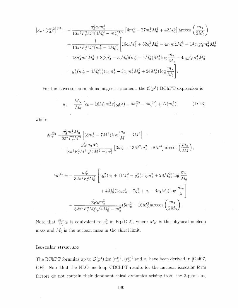
2 3([ - (r4)2((4) - g-c M 2/ [4 - 27m7Mr + 42M] arccos m
167 2 rM (4M - m2 3/2 2Mo)
+ 2F72 4 2 - 4A2) 16c4Mo + 52g AI( - 4c4muM - 14c 6gm M1672j o (m - 4M/1 )
- 13gm MNo4 + 8(3g2 - c4 Mo)(m2 - 4AI)M4 log + 4c6g2m 4 M2
- ginm - 4M,)(4ccn - 3c6 nM, + 24M4) log .
For the isovector anomalous magnetic moment, the 0(p4 ) BChPT expression is
- M c6 - 1o 2 06 ) + 63) + (4) 0(M3MO C 1Mn 160 V V7
(D. 23)
where
(3) g9A27r~
- 82 rF M3 [(3m2 - 7M2) log M
g 4M2
87 rFM3 _ 4M2 - M2
- 3M2I
[3M4 - 13M 2m2 + 8M 4] arccos
3 2
3 2 2 2~M[4g(C 6 + + 1)M - gA(5c 6rm!
+ 4M (2c6g2 + 7g + c-
2 3g cm " (5m2
327 2 F M 4M -m
+ 28Mg) log
4c4Mo) logn ]
- 16M )arccos m(2Mo)
Note that N C6 is equivalent to K< in Eq.(D.2), where MN is the physical nucleon
mass and MO is the nucleon mass in the chiral limit.
Isoscalar structure
The BChPT formulas up to 0(p4) for (rs)2 , (,I)2 and K, have been derived in [Gai07,
GH]. Note that the NLO one-loop CBChPT results for the nucleon isoscalar form
factors do not contain their dominant chiral dynamics arising from the 3-pion cut,
(M r
V
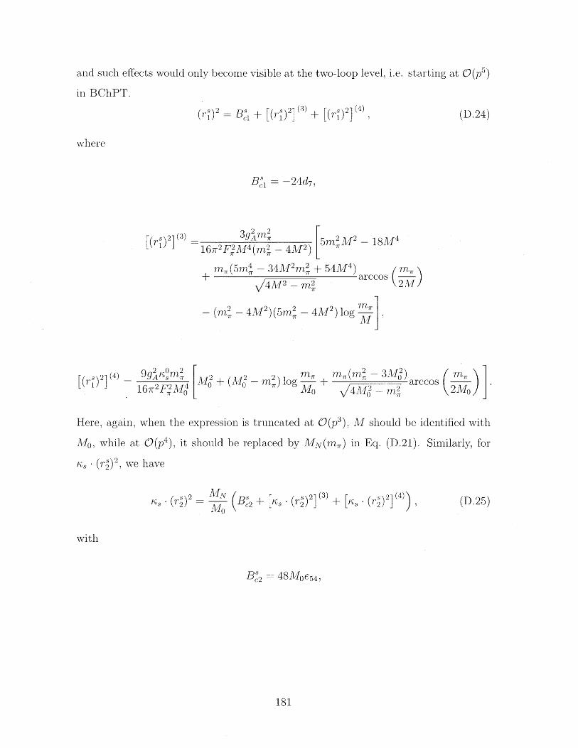
and such effects would only become visible at the two-loop level, i.e. starting at O(p5 )
in BChPT.
(rs)2 = Bs + [(rs)2] ( + [(r)2 ] (4)
where
B = -24d 7 ,
3gm 5m M216r 2F2 M4 (m2 - 4M 2) [
m(5m4 -34M 2m2 + 54M 4)Q4M2 -M2
- 18M 4
maarecos (M
- (M2 - 4M 2)(5m2 - 4M 2 ) log
(r (4) - 9g2irm 0
16 2F2M 4log m + mmi 3M)arcos
Mo Q4M - m2
Here, again, when the expression is truncated at 0(p 3 ), M should be identified with
MO, while at 0(p 4 ), it should be replaced by MN(n) in Eq. (D.21). Similarly, for
(rs)2 , we have
s) (r) 2 MN Be2 + [s (rs) 2] (3) + [n, - (r) 2 ] (4) (D.25)
with
B 2= 48Moe5 4,
181
(D.24)
s)2] (3)
m7
2Mom2 + (M2 - m')2
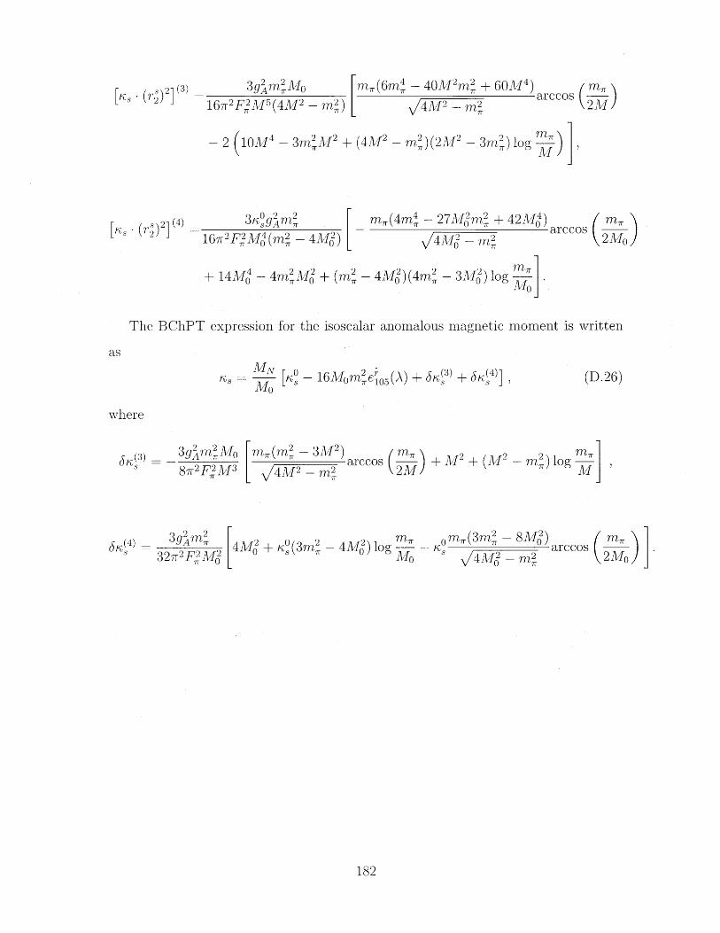
3g2m Mo167 2FM 5 (4M 2 - ml)
mn(6m4 - 40M 2 m + 60M 4) mo
L 4M2 - (2M)
- 2 (1OM4 - 3m2M 2 + (4M 2 - mir)(2M 2 - 3m) log MIT
s)2] (4) 3 g m M 22s ()] 172F2 4d (mT - 4M2)
m (4M4 - 27M( m' + 42MI0)
f4Ms -m
+ 14MO - 4rn M2 + (m 2 - 4M )(4m2 - 3M ) log '.
The BChPT expression for the isoscalar anomalous magnetic moment is written
MNVKS I K - 16MOmn2er5 N A- V,()+ 4 (D.26)
- 3g 2 ri 2MOS 82F2M
M7 (M 2n -3 3M 2 )7F F arccos4M/I 2- ;T ( )+ M2 + (Ml 2
- ml
3g 2m 26(4) = Ag m, 327r2F M02
4M2 + KO(3m2 - 4Mg) log -S 7* Mo- omI(3m - 8MO2) areos
" f4Ms m2,
182
(;.S)2] (3)s (7')2 ]
arcos
where
2Mo
Appendix E
Abbreviations
DWF domain wall fermions
BMW Budapest-Marseille-Wuppertal [collaboration]
(L)QCD (lattice) quantum chromodynamics
CBChPT covariant chiral perturbation theory
HBChPT heavy-baryon chiral perturbation theory
SSE small-scale expansion (HBChPT with A-resonance)
GPD generalized parton distribution(s)
GFF generalized form factor(s)
183
184
Bibliography
[A+88a] L. A. Ahrens et al. A study of the axial vector form-factor and secondclass currents in anti-neutrino quasielastic scattering. Phys. Lett.,B202:284 288, 1988.
[A+88b] J. Ashman et al. A measurement of the spin asymmetry and deter-mination of the structure function g(1) in deep inelastic muon protonscattering. Phys. Lett., B206:364, 1988.
[A+99] K. Ackerstaff et al. Flavor decomposition of the polarized quark distri-butions in the nucleon from inclusive and semi-inclusive deep- inelasticscattering. Phys. Lett., B464:123 -134, 1999.
[A+01) A. Airapetian et al. Measurement of the beam spin azimuthal asym-metry associated with deeply-virtual Compton scattering. Phys. Rev.Lett., 87:182001, 2001.
[A+04a] J. Arrington et al. Two-photon exchange and elastic scattering ofelectrons / positrons on the proton. (Proposal for an experiment atVEPP-3). 2004.
[A+04b] C. Aubin et al. Light hadrons with improved staggered quarks: Ap-proaching the continuum limit. Phys. Rev., D70:094505, 2004.
[A+05] A. Aktas et al. Measurement of deeply virtual Compton scattering atHERA. Eur. Phys. J., C44:1 11, 2005.
[A+07] P. Abbon et al. The COMPASS Experiment at CERN. Nucl. Instrum.Meth., A577:455 518, 2007.
[A+08a] C. Allton et al. Physical Results from 2+1 Flavor Domain Wall QCDand SU(2) Chiral Perturbation Theory. Phys. Rev., D78:114509, 2008.
[A+08b] C. Amsler et al. Review of particle physics. Phys. Lett., B667:1, 2008.
[AK+04] A. Ali Khan et al. The nucleon mass in N(f) = 2 lattice QCD: Finitesize effects from chiral perturbation theory. Nucl. Phys., B689:175194, 2004.
185
[AK+06] A. Ali Khan et al. Axial coupling constant of the nucleon for twoflavours of dynamical quarks in finite and infinite volume. Phys. Rev.,D74:094508, 2006.
[AKNT06] C. Alexandrou, G. Koutsou, John W. Negele, and A. Tsapalis. Thenucleon electromagnetic form factors from lattice QCD. Phys. Rev.,D74:034508, 2006.
[AMT07] J. Arrington, W. Melnitehouk, and J. A. Tjon. Global analysis ofproton elastic form factor data with two-photon exchange corrections.Phys. Rev., C76:035205, 2007.
[Are06] H. J. Arends. Overview of the physics at MAMI (Mainz). AIP Conf.Proc., 870:481 485, 2006.
[B+73] Elliott D. Bloom et al. Measurements of inelastic electron scatteringcross-sections near one pion threshold. Phys. Rev. Lett., 30:1186, 1973.
[B+91] V. G. Bornyakov et al. The Density of monopoles in SU(2) lattice
gauge theory. Phys. Lett., B261:116 122, 1991.
[B+98] Claude W. Bernard et al. Quenched hadron spectroscopy with im-proved staggered quark action. Phys. Rev., D58:014503, 1998.
[B+01] Claude W. Bernard et al. The QCD spectrum with three quark flavors.Phys. Rev., D64:054506, 2001.
[B+02] T. Blum et al. Non-perturbative renormalisation of domain wallfermions: Quark bilinears. Phys. Rev., D66:014504, 2002.
[B+04] T. Blum et al. Quenched lattice QCD with domain wall fermions andthe chiral limit. Phys. Rev., D69:074502, 2004.
[B+08a] P. A. Boyle et al. Parton Distribution Amplitudes and Non-Perturbative Renormalisation. PoS, LATTICE2008:165, 2008.
[B+08b] J. D. Bratt et al. Aspects of Precision Calculations of Nucleon Gen-eralized Form Factors with Domain Wall Fermions on an Asqtad Sea.PoS, LATTICE2008:141, 2008.
[B+09] A. Bazavov et al. Full nonperturbative QCD simulations with 2+1flavors of improved staggered quarks. 2009.
[B+10] Jonathan D. Bratt et al. Nucleon structure from mixed action cal-culations using 2+1 flavors of asqtad sea and domain wall valencefermions. 2010.
186
[BBCR95] Giuseppe Beccarini, Massimo Bianchi, Stafano Capitani, and Gian-carlo Rossi. Deep inelastic scattering in improved lattice QCD. 2.The second moment of structure functions. Nuel. Phys., B456:271295, 1995.
[BCS09a] Gunnar Bali, Sara Collins, and Andreas Schafer. Strangeness andcharm content of the nucleon. 2009.
[BCSO9b] Gunnar S. Bali, Sara Collins, and Andreas Schafer. Effective noisereduction techniques for disconnected loops in Lattice QCD. 2009.
[BCT98] J. Bijnens, G. Colangelo, and P. Talavera. The vector and scalar formfactors of the pion to two loops. JHEP, 05:014, 1998.
[BDHS] Claude W. Bernard, Terrence Draper, G. Hockney, and A. Soni. Cal-culation of weak matrix elements: some technical aspects. In *Wup-pertal 1985, Proceedings, Lattice Gauge Theory*, 199-207.
[BEM02] Veronique Bernard, Latifa Elouadrhiri, and Ulf. G. Meissner. Axialstructure of the nucleon. J. Phys., G28:R1 R35, 2002.
[Ber08] J. C. Bernauer. Nucleon form factor measurements in Mainz: Pastand future. Lect. Notes Phys., 745:79- 91, 2008.
[Bet09] Siegfried Bethke. The 2009 World Average of ac(Mz). Eur. Phys. J.,C64:689 703, 2009.
[BF75] Stanley J. Brodsky and Glennys R. Farrar. Scaling laws for large-momentum-transfer processes. Phys. Rev. D, 11(5):1309 1330, Mar1975.
[BF89] Douglas S. Beder and Harold W. Fearing. Further comments on ra-diative muon capture in hydrogen and nucleon excitation. Phys. Rev.,D39:3493-3496, 1989.
[BFHM98] Veronique Bernard, Harold W. Fearing, Thomas R. Hemmert, andUlf G. MeiBner. The form factors of the nucleon at small momentumtransfer. Nucl. Phys., A635:121 145, 1998.
[BHM05] Veronique Bernard, Thomas R. Hemmert, and Ulf-G. Meifner. Chiralextrapolations and the covariant small scale expansion. Phys. Lett.,B622:141 150, 2005.
[BHM07] M. A. Belushkin, H. W. Hammer, and Ulf-G. MeiBner. Dispersionanalysis of the nucleon form factors including meson continua. Phys.Rev., C75:035202, 2007.
187
Stanley J. Brodsky, Dae Sung Hwang, Bo-Qiang Ma, and IvanSchmidt. Light-cone representation of the spin and orbital angularmomentum of relativistic composite systems. Nucl. Phys., B593:311335, 2001.
[Bis05] Bojan Bistrovie. Perturbative renormalization of proton observablesin lattice QCD using domain wall fermions. PhD thesis, MIT, 2005.
[BJ97] Ian Balitsky and Xiang-Dong Ji. How much of the nucleon spin iscarried by glue? Phys. Rev. Lett., 79:1225 1228, 1997.
[BJY03] Andrei V. Belitsky, Xiang-dong Ji, and Feng Yuan. A perturbativeQCD analysis of the nucleon's Pauli form factor F2(Q**2). Phys. Rev.Lett., 91:092003, 2003.
[BKKM92] Veronique Bernard, Norbert Kaiser, Joachim Kambor, and Ulf G.Meissner. Chiral structure of the nucleon. Nucl. Phys., B388:315-345, 1992.
[BKM94] V. Bernard, Norbert Kaiser, and Ulf G. Meissner. QCD accuratelypredicts the induced pseudoscalar coupling constant. Phys. Rev.,D50:6899 6901, 1994.
[BKM97] V. Bernard, Norbert Kaiser, and Ulf-G. Meiflner. Determination ofthe low-energy constants of the next-to- leading order chiral pion nu-cleon Lagrangian. Nucl. Phys., A615:483-500, 1997.
[BL99] Thomas Becher and H. Leutwyler. Baryon chiral perturbation theoryin manifestly Lorentz invariant form. Eur. Phys. J., C9:643-671, 1999.
[Bra09] J. D. Bratt. PhD thesis, MIT, 2009.
[BurO0] Matthias Burkardt. Impact parameter dependent parton distribu-tions and off-forward parton distributions for zeta - 0. Phys. Rev.,D62:071503(R), 2000.
[Bur03] Matthias Burkardt. Impact parameter space interpretation for gener-alized parton distributions. Int. J. Mod. Phys., A18:173 208, 2003.
[C+93] Seonho Choi et al. Axial and pseudoscalar nucleon form-factors fromlow- energy pion electroproduction. Phys. Rev. Lett., 71:3927 3930,1993.
[C+03] S. Chekanov et al. Measurement of deeply virtual Compton scatteringat HERA. Phys. Lett., B573:46 62, 2003.
[CD04] Gilberto Colangelo and Stephan Dirr. The pion mass in finite volume.Eur. Phys. J., C33:543 553, 2004.
[BHMS01]
[CKS97] K. G. Chetyrkin, Bernd A. Kniehl, and M. Steinhauser. Strong cou-pling constant with flavour thresholds at four loops in the MS-barscheme. Phys. Rev. Lett., 79:2184 2187, 1997.
[col] BMW collaboration. in preparation.
[CR00] K. G. Chetyrkin and A. Retey. Renormalization and running of quarkmass and field in the regularization invariant and MS-bar schemes atthree and four loops. Nucl. Phys., B583:3 34, 2000.
[D+02] D. Dolgov et al. Moments of nucleon light cone quark distributionscalculated in full lattice QCD. Phys. Rev., D66:034506, 2002.
[D+08] S. Durr et al. Ab-Initio Determination of Light Hadron Masses. Sci-ence, 322:1224 1227, 2008.
[D+09] Takumi Doi et al. Nucleon strangeness form factors from Nf = 2 + 1clover fermion lattice QCD. Phys. Rev., D80:094503, 2009.
[DDG] Durham University (UK) Durham Database Group.
[dF+00] P. de Forcrand et al. Renormalization group flow of SU(3) latticegauge theory: Numerical studies in a two coupling space. Nucl. Phys.,B577:263 278, 2000.
[DFJK05] M. Diehl, Th. Feldmann, R. Jakob, and P. Kroll. Generalized partondistributions from nucleon form factor data. Eur. Phys. J., C39:1 39,2005.
[DGH08] Marina Dorati, Tobias A. Gail, and Thomas R. Hemmert. ChiralPerturbation Theory and the first moments of the Generalized PartonDistributions in a Nucleon. Nucl. Phys., A798:96 131, 2008.
[DieO3] M. Diehl. Generalized parton distributions. Phys. Rept., 388:41 277,2003.
[DMS07] M. Diehl, A. Manashov, and A. Schafer. Generalized parton distri-butions for the nucleon in chiral perturbation theory. Eur. Phys. J.,A31:335 355, 2007.
[DMW91] R. M. Davidson, N. C. Mukhopadhyay, and R. S. Wittman. EffectiveLagrangian approach to the theory of pion photoproduction in theDelta (1232) region. Phys. Rev., D43:71 94, 1991.
[DolOO] D. Dolgov. Calculation of the Structure of the Proton using LatticeQCD. PhD thesis, MIT, 2000.
[E+06a] R. G. Edwards et al. Nucleon structure in the chiral regime with do-main wall fermions on an improved staggered sea. PoS, LAT2006:121,2006.
189
R. G. Edwards et al. The nucleon axial charge in full lattice QCD.Phys. Rev. Lett., 96:052001, 2006.
[EHK98] R. G. Edwards, Urs M. Heller, and T. R. Klassen. The effectivenessof non-perturbative O(a) improvement in lattice QCD. Phys. Rev.Lett., 80:3448 3451, 1998.
[EM02] D. R. Entem and R. Machleidt. Chiral 2pi exchange at order four andperipheral N N scattering. Phys. Rev., C66:014002, 2002.
[FJ01J B. W. Filippone and Xiang-Dong Ji. The spin structure of the nucleon.Adv. Nucl. Phys., 26:1, 2001.
[FMS98] Nadia Fettes, Ulf-G. Meiifner, and Sven Steininger. Pion nucleonscattering in chiral perturbation theory. I: Isospin-symmetric case.Nucl. Phys., A640:199 234, 1998.
[FPPT85) M. Falcioni, M. L. Paciello, G. Parisi, and B. Taglienti. Again onSU(3) glueball mass. Nucl. Phys., B251:624 -632, 1985.
[FW03] J. Friedrich and T. Walcher. A coherent interpretation of the formfactors of the nucleon in terms of a pion cloud and constituent quarks.Eur. Phys. J., A17:607-623, 2003.
[G+89] S. G~isken et al. Nonsinglet axial vector couplings of the baryon octetin lattice qcd. Phys. Lett., B227:266, 1989.
[G90) S. Gisken. A Study of smearing techniques for hadron correlationfunctions. Nucl. Phys. Proc. Suppl., 17:361 364, 1990.
[G+96a] M. Gockeler et al. Lattice Operators for Moments of the StructureFunctions and their Transformation under the Hypercubic Group.Phys. Rev., D54:5705 5714, 1996.
[G+96b] M. Gockeler et al. Perturbative Renormalization of Lattice BilinearQuark Operators. Nucl. Phys., B472:309 333, 1996.
[G+01] 0. Gayou et al. Measurements of the elastic electromagnetic formfactor ratio mu pGEp/GMp via polarization transfer. Phys. Rev.,C64:038202, 2001.
[G+02] 0. Gayou et al. Measurement of G(E(p))/G(M(p)) in e(pol.) p-> ep(pol.) to Q2 = 5.6 GeV2 . Phys. Rev. Lett., 88:092301, 2002.
[G+05a] M. Gockeler et al. Investigation of the second moment of the nucleon'sg1 and g2 structure functions in two-flavor lattice QCD. Phys. Rev.,D72:054507, 2005.
[G+05b] M. G6ckeler et al. Nucleon electromagnetic form factors on the latticeand in chiral effective field theory. Phys. Rev., D71:034508, 2005.
190
[E+06b]
[G+10] M. Gockeler et al. Perturbative and Nonperturbative Renormalizationin Lattice QCD. 2010.
[Gai07] T. Gail. Chiral Analysis and Baryon Form Factors. PhD thesis,Technical University Munich, 2007.
[GH] T. A. Gail and T. R. Hemmert. Quark-mass dependence of the formfactors of the nucleon near the photon point. forthcoming.
[Gia1O] Paola Gianotti. The PANDA experiment at FAIR. Nucl. Phys.,A835:96 101, 2010.
[GPGASvB94] Margarita Garcia Perez, Antonio Gonzalez-Arroyo, Jeroen R. Snippe,and Pierre van Baal. Instantons from over - improved cooling. Nucl.Phys., B413:535 552, 1994.
[GPVO1] K. Goeke, Maxim V. Polyakov, and M. Vanderhaeghen. Hard Exclu-sive Reactions and the Structure of Hadrons. Prog. Part. Nucl. Phys.,47:401 515, 2001.
[Gra92] J. M. Grandy. Investigation of hadronic structure by solving QCD ona lattice. PhD thesis, MIT, 1992.
[Gra03a] J. A. Gracey. Three loop anomalous dimension of non-singlet quarkcurrents in the RI' scheme. Nucl. Phys., B662:247 278, 2003.
[Gra03b] J. A. Gracey. Three loop anomalous dimension of the second momentof the transversity operator in the MS-bar and RI' schemes. Nucl.Phys., B667:242-260, 2003.
[Gra06] J. A. Gracey. Three loop anomalous dimensions of higher momentsof the non-singlet twist-2 Wilson and transversity operators in theMSbar and RI' schemes. JHEP, 10:040, 2006.
[GSS88] J. Gasser, M. E. Sainio, and A. Svarc. Nucleons with Chiral Loops.Nucl. Phys., B307:779, 1988.
[GT58a] M. L. Goldberger and S. B. Treiman. Decay of the pi meson. Phys.Rev., 110:1178 1184, 1958.
[GT58b] M. L. Goldberger and S. B. Treiman. Form-factors in Beta decay andmuon capture. Phys. Rev., 111:354 361, 1958.
[Gup97] Rajan Gupta. Introduction to lattice QCD. 1997.
[GV98] Pierre A. M. Guichon and M. Vanderhaeghen. Virtual Compton scat-tering off the nucleon. Prog. Part. Nucl. Phys., 41:125 190, 1998.
[H+76] G. H6hler et al. Analysis of Electromagnetic Nucleon Form-Factors.Nucl. Phys., B114:505, 1976.
191
Philipp Hagler et al. Moments of nucleon generalized parton distri-butions in lattice QCD. Phys. Rev., D68:034505, 2003.
[H+08] Ph. Hagler et al. Nucleon Generalized Parton Distributions from FullLattice QCD. Phys. Rev., D77:094502, 2008.
[HHK97] Thomas R. Hemmert, Barry R. Holstein, and Joachim Kambor. Sys-tematic 1/M expansion for spin 3/2 particles in baryon chiral pertur-bation theory. Phys. Lett., B395:89 95, 1997.
[HHK98] Thomas R. Hemmert, Barry R. Holstein, and Joachim Kambor. Chi-ral Lagrangians and Delta(1232) interactions: Formalism. J. Phys.,G24:1831- 1859, 1998.
[HN94] P. Hasenfratz and F. Niedermayer. Perfect lattice action for asymp-totically free theories. Nucl. Phys., B414:785 814, 1994.
[HPW03] Thomas R. Hemmert, Massimiliano Procura, and Wolfram Weise.Quark mass dependence of the nucleon axial-vector coupling constant.Phys. Rev., D68:075009, 2003.
[HW02] Thomas R. Hemmert and Wolfram Weise. Chiral magnetism of thenucleon. Eur. Phys. J., A15:487-504, 2002.
[ILS+86] Ernst-Michael Ilgenfritz, M. L. Laursen, G. Schierholz, M. Muller-Preussker, and H. Schiller. First Evidence for the Existence of Instan-tons in the Quantized SU(2) Lattice Vacuum. Nucl. Phys., B268:693,1986.
[Iwa85] Y. Iwasaki. Renormalization Group Analysis of Lattice Theories andImproved Lattice Action: Two-Dimensional Nonlinear O(N) SigmaModel. Nucl. Phys., B258:141 156, 1985.
[J+96] G. Jonkmans et al. Radiative muon capture on hydrogen and theinduced pseudoscalar coupling. Phys. Rev. Lett., 77:4512 -4515, 1996.
[Ji97] Xiang-Dong Ji. Gauge invariant decomposition of nucleon spin. Phys.Rev. Lett., 78:610-613, 1997.
[Ji98] Xiang-Dong Ji. Off-forward parton distributions. J. Phys., G24:11811205, 1998.
[K+90] T. Kitagaki et al. Study of neutrino d -> mu- p p(s) and neutrino d-> mu- Delta++ (1232) n(s) using the BNL 7-foot deuterium filledbubble chamber. Phys. Rev., D42:1331-1338, 1990.
[Kap92) David B. Kaplan. A Method for simulating chiral fermions on thelattice. Phys. Lett., B288:342 347, 1992.
192
[H+03]
[Kel04] J. J. Kelly. Simple parametrization of nucleon form factors. Phys.Rev., C70:068202, 2004.
[KLN+69] R. L. Kustom, D. E. Lundquist, T. B. Novey, A. Yokosawa, andF. Chilton. Quasielastic neutrino scattering. Phys. Rev. Lett.,22:1014 1017, 1969.
[KN02] V. A. Korotkov and W. D. Nowak. Future measurements of deeplyvirtual Compton scattering at HERMES. Eur. Phys. J., C23:455 461,2002.
[LBO+08] Huey-Wen Lin', Tom Blum, Shigemi Ohta, Shoichi Sasaki, and TakeshiYamazaki. Nucleon structure with two flavors of dynamical domain-wall fermions. Phys. Rev., D78:014505, 2008.
[LCE+10] Huey-Wen Lin, Saul D. Cohen, Robert G. Edwards, Kostas Orginos,and David G. Richards. Lattice Calculations of Nucleon Electromag-netic Form Factors at Large Momentum Transfer. 2010.
[Lep] G. Peter Lepage. The analysis of algorithms for lattice field theory.Invited lectures given at TASI'89 Summer School, Boulder, CO, Jun4-30, 1989.
[LHP] LHP collaboration. in preparation.
[LM93] G. Peter Lepage and Paul B. Mackenzie. On the viability of latticeperturbation theory. Phys. Rev., D48:2250 2264, 1993.
[Lus77] M. Luscher. Construction of a Selfadjoint, Strictly Positive TransferMatrix for Euclidean Lattice Gauge Theories. Commun. Math. Phys.,54:283, 1977.
[LW90] Martin Luscher and Ulli Wolff. How to calculate the elastic scatter-ing matrix in two-dimensional quantum field theories by numericalsimulation. Nucl. Phys., B339:222 252, 1990.
[M+98] B. D. Milbrath et al. A comparison of polarization observables inelectron scattering from the proton and deuteron. Phys. Rev. Lett.,80:452 455, 1998.
[MM] I. Montvay and G. Munster. Quantum fields on a lattice. Cambridge,UK: Univ. Pr. (1994) 491 p. (Cambridge monographs on mathemati-cal physics).
[MMD96] P. Mergell, Ulf G. MeiBner, and D. Drechsel. Dispersion-TheoreticalAnalysis of the Nucleon Electromagnetic Fornfactors. Nucl. Phys.,A596:367 396, 1996.
193
[MPS+95] G. Martinelli, C. Pittori, Christopher T. Sachrajda, M. Testa, andA. Vladikas. A General method for nonperturbative renormalizationof lattice operators. Nucl. Phys., B445:81 108, 1995.
[NN81] Holger Bech Nielsen and M. Ninomiya. No Go Theorem for Regular-izing Chiral Fermions. Phys. Lett., B105:219, 1981.
[NN93] Rajamani Narayanan and Herbert Neuberger. Chiral fermions on thelattice. Phys. Rev. Lett., 71:3251 3254, 1993.
[OLY09] OLYMPUS Collaboration. An Experiment to Definitively Determinethe Contribution of Multiple Photon Exchange in Elastic Lepton-Nucleon Scattering. http://web.mit.edu/olympus/, 2009.
[OT99] Kostas Orginos and Doug Toussaint. Testing improved actions fordynamical Kogut-Susskind quarks. Phys. Rev., D59:014501, 1999.
[OTS99] Kostas Orginos, Doug Toussaint, and R. L. Sugar. Variants of fatten-ing and flavor symmetry restoration. Phys. Rev., D60:054503, 1999.
[OY08] Shigemi Ohta and Takeshi Yamazaki. Nucleon structure with dynam-ical (2+1)-flavor domain wall fermions lattice QCD. 2008.
[P+01] T. Pospischil et al. Measurement of G(E(p))/G(M(p)) via polarizationtransfer at Q2 = 0.4 GeV/c 2 . Eur. Phys. J., A12:125-127, 2001.
[P+05] V. Punjabi et al. Proton elastic form factor ratios to Q2 = 3.5 GeV 2
by polarization transfer. Phys. Rev., C71:055202, 2005.
[P+10] Randolf Pohl et al. The size of the proton. Nature, 466(7303):213 216,2010.
[PMHW07] M. Procura, B. U. Musch, T. R. Hemmert, and W. Weise. Chiralextrapolation of gA with explicit A(1232) degrees of freedom. Phys.Rev., D75:014503, 2007.
[PMW+06] M. Procura, B. U. Musch, T. Wollenweber, T. R. Hemmert, andW. Weise. Nucleon mass: From lattice QCD to the chiral limit. Phys.Rev., D73:114510, 2006.
[PS] A.V. Pochinsky and S. N. Syritsyn. In private communications.
[RBC07] RBC and LHP collaborations. Simulations with dynamical domainwall fermions. USQCD resource allocation proposal, 2007.
[RenO4] D. B. Renner. Exploring Proton Structure using Lattice QCD. PhDthesis, MIT, 2004.
[Rot05] H. J. Rothe. Lattice gauge theories: An Introduction. World Sci.Lect. Notes Phys., 74:1-605, 2005.
194
[S+01] S. Stepanyan et al. First observation of exclusive deeply virtual Comp-ton scattering in polarized electron beam asyimnetry measurements.Phys. Rev. Lett., 87:182002, 2001.
[S+09] C. Sturm et al. Renormalization of quark bilinear operators in amomentum- subtraction scheme with a nonexceptional subtractionpoint. Phys. Rev., D80:014501, 2009.
[S+10] S. N. Syritsyn et al. Nucleon Electromagnetic Form Factors from Lat-tice QCD using 2+1 Flavor Domain Wall Fermnions on Fine Latticesand Chiral Perturbation Theory. Phys. Rev. D, 81(3):034507, Feb2010.
[Sha93] Yigal Shamir. Chiral fermions from lattice boundaries. Nucl. Phys.,B406:90 106, 1993.
[Sha07] Stephen R. Sharpe. Future of Chiral Extrapolations with DomainWall Fermions. 2007.
[SN07] Sergey Syritsyn and John W. Negele. Oscillatory terms in the domainwall transfer matrix. PoS, LAT2007:078, 2007.
[Ste33] 0. Stern. Nature, 132:169, 1933.
[SW85] B. Sheikholeslami and R. Wohlert. Improved Continuum Limit Lat-tice Action for QCD with Wilson Fermions. Nucl. Phys., B259:572,1985.
[Tho08] Anthony W. Thomas. Interplay of Spin and Orbital Angular Momen-tum in the Proton. Phys. Rev. Lett., 101:102003, 2008.
[Vog04) Werner Vogelsang. QCD spin physics: Status, and prospects forRHIC. Pramana, 63:1251, 2004.
[W+98] D. H. Wright et al. Measurement of the induced pseudoscalar couplingusing radiative muon capture on hydrogen. Phys. Rev., C57:373-390,1998.
[Wil74] Kenneth G. Wilson. Confinement of quarks. Phys. Rev., D10:2445-2459, 1974.
[WL+09] A. Walker-Loud et al. Light hadron spectroscopy using domain wallvalence quarks on an Asqtad sea. Phys. Rev., D79:054502, 2009.
[Y+09] Takeshi Yamazaki et al. Nucleon form factors with 2+1 flavor dy-namical domain-wall fermions. Phys. Rev., D79:114505, 2009.
[Zic77] A. Zichichi, editor. New Phenomena in Subnuclear Physics. PlenumPress, 1977.
195
Related Documents