Exploiting Graph and Geodesic Distance Constraint for Deep ...

�����������������

Citation: Fang, X.; Li, Q.; Li, Q.; Ding,

K.; Zhu, J. Exploiting Graph and

Geodesic Distance Constraint for

Deep Learning-Based Visual

Odometry. Remote Sens. 2022, 14,

1854. https://doi.org/10.3390/

rs14081854

Academic Editors: Yangquan Chen,

Subhas Mukhopadhyay, Nunzio

Cennamo, M. Jamal Deen, Junseop

Lee and Simone Morais

Received: 2 March 2022

Accepted: 9 April 2022

Published: 12 April 2022

Publisher’s Note: MDPI stays neutral

with regard to jurisdictional claims in

published maps and institutional affil-

iations.

Copyright: © 2022 by the authors.

Licensee MDPI, Basel, Switzerland.

This article is an open access article

distributed under the terms and

conditions of the Creative Commons

Attribution (CC BY) license (https://

creativecommons.org/licenses/by/

4.0/).

remote sensing

Article

Exploiting Graph and Geodesic Distance Constraint for DeepLearning-Based Visual OdometryXu Fang 1,2, Qing Li 1,3, Qingquan Li 1,3, Kai Ding 4 and Jiasong Zhu 3,5,*

1 Guangdong Key Laboratory of Urban Informatics, Shenzhen University, Shenzhen 518060, China;[email protected] (X.F.); [email protected] (Q.L.); [email protected] (Q.L.)

2 College of Electronics and Information Engineering, Shenzhen University, Shenzhen 518060, China3 College of Civil and Transportation Engineering, Shenzhen University, Shenzhen 518060, China4 School of Computer Science and Technology, Dongguan University of Technology, Dongguan 523808, China;

[email protected] Shenzhen University Branch, Shenzhen Institute of Artificial Intelligence and Robotics for Society,

Shenzhen 518060, China* Correspondence: [email protected]

Abstract: Visual odometry is the task of estimating the trajectory of the moving agents from con-secutive images. It is a hot research topic both in robotic and computer vision communities andfacilitates many applications, such as autonomous driving and virtual reality. The conventionalodometry methods predict the trajectory by utilizing the multiple view geometry between consecu-tive overlapping images. However, these methods need to be carefully designed and fine-tuned towork well in different environments. Deep learning has been explored to alleviate the challenge bydirectly predicting the relative pose from the paired images. Deep learning-based methods usuallyfocus on the consecutive images that are feasible to propagate the error over time. In this paper,graph loss and geodesic rotation loss are proposed to enhance deep learning-based visual odometrymethods based on graph constraints and geodesic distance, respectively. The graph loss not onlyconsiders the relative pose loss of consecutive images, but also the relative pose of non-consecutiveimages. The relative pose of non-consecutive images is not directly predicted but computed fromthe relative pose of consecutive ones. The geodesic rotation loss is constructed by the geodesicdistance and the model regresses a Lie algebra so(3) (3D vector). This allows a robust and stableconvergence. To increase the efficiency, a random strategy is adopted to select the edges of the graphinstead of using all of the edges. This strategy provides additional regularization for training thenetworks. Extensive experiments are conducted on visual odometry benchmarks, and the obtainedresults demonstrate that the proposed method has comparable performance to other supervisedlearning-based methods, as well as monocular camera-based methods. The source code and theweight are made publicly available.

Keywords: deep learning; graph constraints; visual odometry; geodesic distance

1. Introduction

Visual odometry (VO) is the task of estimating the trajectory of mobile agents (e.g.,robots, vehicles, and unmanned aerial vehicles (UAVs)) from image sequences. It is oneof the fundamental and important remote sensing methods in autonomous driving, pho-togrammetry, and virtual/augmented reality (VR, AR) applications. In the past few decades,visual odometry has attracted significant interest in both robotics and computer visioncommunities [1]. Visual odometry was first proposed in 2004 by Nister [2] for the navi-gation of autonomous ground vehicles. Later, monocular visual navigation was achievedfor autonomous micro helicopters [3]. Visual odometry is also a promising supplement toother localization technologies, such as inertial measurement unit (IMU), global positioningsystem (GPS), LiDAR and ultrasonic rangefinder especially in GPS-denied environments,

Remote Sens. 2022, 14, 1854. https://doi.org/10.3390/rs14081854 https://www.mdpi.com/journal/remotesensing

Remote Sens. 2022, 14, 1854 2 of 19

such as tunnels, underwater, and indoor scenarios [4–6]. The IMU is a lightweight, low-costsensor that can improve the motion tracking performance of visual sensors by integratingthe IMU measurements. The ultrasonic rangefinder can provide the backup for the LiDARrangefinder, due to the LiDAR beam being narrow. Fusing the advantages of differentremote sensing techniques can enhance the reliability of the system. The performance ofvisual odometry is important for various artificial intelligence applications.

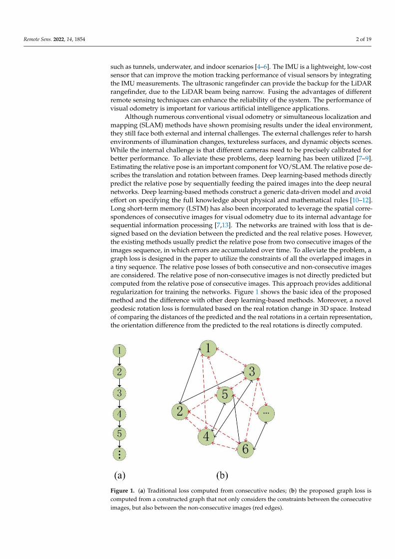
Although numerous conventional visual odometry or simultaneous localization andmapping (SLAM) methods have shown promising results under the ideal environment,they still face both external and internal challenges. The external challenges refer to harshenvironments of illumination changes, textureless surfaces, and dynamic objects scenes.While the internal challenge is that different cameras need to be precisely calibrated forbetter performance. To alleviate these problems, deep learning has been utilized [7–9].Estimating the relative pose is an important component for VO/SLAM. The relative pose de-scribes the translation and rotation between frames. Deep learning-based methods directlypredict the relative pose by sequentially feeding the paired images into the deep neuralnetworks. Deep learning-based methods construct a generic data-driven model and avoideffort on specifying the full knowledge about physical and mathematical rules [10–12].Long short-term memory (LSTM) has also been incorporated to leverage the spatial corre-spondences of consecutive images for visual odometry due to its internal advantage forsequential information processing [7,13]. The networks are trained with loss that is de-signed based on the deviation between the predicted and the real relative poses. However,the existing methods usually predict the relative pose from two consecutive images of theimages sequence, in which errors are accumulated over time. To alleviate the problem, agraph loss is designed in the paper to utilize the constraints of all the overlapped images ina tiny sequence. The relative pose losses of both consecutive and non-consecutive imagesare considered. The relative pose of non-consecutive images is not directly predicted butcomputed from the relative pose of consecutive images. This approach provides additionalregularization for training the networks. Figure 1 shows the basic idea of the proposedmethod and the difference with other deep learning-based methods. Moreover, a novelgeodesic rotation loss is formulated based on the real rotation change in 3D space. Insteadof comparing the distances of the predicted and the real rotations in a certain representation,the orientation difference from the predicted to the real rotations is directly computed.

Figure 1. (a) Traditional loss computed from consecutive nodes; (b) the proposed graph loss iscomputed from a constructed graph that not only considers the constraints between the consecutiveimages, but also between the non-consecutive images (red edges).

Remote Sens. 2022, 14, 1854 3 of 19

The main contributions of this paper are as follows:

• A graph loss is proposed to fully exploit the constraints of a tiny image sequence toreplace the conventional loss module based on two consecutive images, which canalleviate the accumulating errors in visual odometry. Moreover, the proposed graphloss leads to more constraints to regularize the network.

• A new representation of rotation loss is designed based on the geodesic distance, which ismore robust than the usual methods that use the angles difference in Euclidean distance.

• Extensive experiments are conducted to demonstrate the superiority of the proposedlosses. Furthermore, the effects of different sliding window sizes and sequence over-lapping are also analyzed.

The remainder of the paper is organized as follows: Section 2 presents an overview ofrelated works on visual odometry. Section 3 describes the proposed method and the lossfunctions. The experiments are presented in Section 4. Section 5 discusses the effects indifferent experimental settings. Section 6 concludes the paper.

2. Related Work

The various approaches and frameworks proposed for visual odometry can be dividedinto two categories: geometry-based methods and learning-based methods.

2.1. Geometry-Based Methods

Geometry-based methods estimate the relative pose between frame-to-frame basedon the stereo view geometry. A typical pipeline of the geometry-based method containscamera calibration [14], feature extraction [15], feature matching, outlier removal, andoptimization module [16–18]. Based on this theory, numerous visual odometry algorithmsand SLAM systems have been created, demonstrating exceptional performance [19], suchas VINS-MONO [20], ORB-SLAM3 [21], and Kimera-VIO [22]. These methods are robustand versatile visual or visual-inertial odometry methods that utilize the image data andother sensor data. Zhang et al. [23] proposed a series of optimal methods that made 3D re-construction and mapping systems more robust and accurate. Generally, the two dominantgeometry-based methods are feature-based methods and direct methods. The feature-basedmethods use various feature detectors, including FAST [24], SURF [25], BRIEF [26], andcorner detectors [27], to detect the salient features. The feature point tracker is used to trackthese feature points in the next image of the same sequence. Mono-SLAM [28] simulta-neously estimates the camera motion and the 3D structure of an unknown environmentin real-time. LIBVISO2 [29] employs multi-view geometry to estimate relative pose byextracting and tracking the salient feature points. One of the most successful and classicalSLAM systems is ORB-SLAM2 [30] that was adapted to maintain a feature map for driftcorrection along with pose estimation. However, the sparse feature-based methods arecomputationally expensive and do not utilize the information of the whole image.

The direct methods utilize all the pixels and optimize geometry errors for pose estima-tion between consecutive images under the assumption of photometric consistency [31].To improve the computational efficiency, the Direct Sparse Odometry (DSO) [32] adoptedsparse and direct methods for the monocular camera and demonstrated robustness forphotometric consistency. Although many geometry-based methods have shown goodperformance in good environments, they tend to fail in textureless environments ordifferent illuminations.

2.2. Deep Learning-Based Methods

Motivated by the good performance in object detection and classification [33–36],deep learning techniques have been introduced to address the problems of traditionalcamera location methods [37]. K. R. Konda et al. [38] formulated visual odometry asa classification problem. They were the first to apply deep learning methods to visualodometry. The deep learning model was used to predict the velocity and direction withestimated depth from stereo images due to the effective feature representation of the

Remote Sens. 2022, 14, 1854 4 of 19

deep learning model [39,40]. The PoseNet [41] considers the camera relocation as a poseregression problem; a convolutional neural network (CNN) built on the GoogLeNet modelis used to regress the six degrees of freedom (6-DoF) camera pose from a single RGB imagein an end-to-end manner. The KFNet improved the learning-based camera re-localizationmethod by incorporating Kalman filtering [42].

In [43], an image localization has been proposed based on a deep learning methodwith the pose correction by matching the map inferred from images and local map extractfrom 3D map. The main disadvantage of this method is that it needs to be re-trainedor at least fine-tuned for a new environment, limiting its widespread applications. Toaddress this issue, frame-to-frame Ego-Motion estimation based on CNN was proposedin [44], which achieved robust performance under the challenging scene. However, it is atime-consuming process since the model takes dense optical flow rather than RGB imagedata as input. Flowdometry [45] cast the visual odometry as a regression problem usingthe FlowNet [46] to extract the optical flow information and a fully connected layer todirectly predict camera translation and rotation. DeepVO [7] regarded visual odometry asa sequential modeling problem and fed image sequences or videos into a network designedbased on CNN and recurrent neural network (RNN) in an end-to-end framework. ESP-VO [47] presented a sequence-to-sequence probabilistic visual odometry framework basedon DeepVO and predicted the poses and uncertainties of image sequences or videos. M. R.U. Saputra et al. [8] presented a curriculum learning strategy for learning the geometry ofmonocular visual odometry and constructed geometry-aware objective function by jointlyoptimizing relative and composite transformations over small windows. Recently, someunsupervised learning-based VO methods have also achieved comparable performances.SC-Sfmlearner [48] achieved the scale consistent on a long video sequence by geometryconsistency loss and provided full camera trajectory. TrajNet [49] proposed a novel pose-to-trajectory constraint and improved the view reconstruction constraint to constrain thetraining process. The above-mentioned methods utilize stereo images and perform depthestimation jointly with visual odometry, which increases the complexity of these methods.

The method proposed in this paper also belongs to sequential deep learning-basedmethods. The main difference is that the proposed method utilizes the constraints of animage sequence to further regularize the network.

3. Deep Learning-Based Visual Odometry with Graph and GeodesicDistance Constraints

In this section, firstly, a brief introduction to the framework of deep learning-basedvisual odometry is presented, and then the network architecture and the proposed lossfunctions are elaborated.

3.1. Deep Learning-Based Visual Odometry

Visual odometry tries to estimate the trajectory from image sequences or videos. Givenimage sequences I1, I2, . . . , In, they sequentially predict relative poses P1,0, P2,1, P3,2, . . . ,Pn,n−1, and the absolute pose of time t is obtained by accumulating the relative poses accord-ing to Equation (1). The trajectory is the absolute pose set of P0, P1, P2, . . . , Pn. Therefore,the vital component is to estimate the relative pose. The relative pose is comprised ofrotation matrix and translation vector.

Pn = P1,0 · P2,1 · P3,2 · · · Pn,n−1 (1)

where Pn,n−1 =

[Rotn,n−1 tn,n−1

0 1

], Rotn,n−1 ∈ SO(3) is the rotation matrix, and tn,n−1 ∈

R3×1 is the translation vector.Deep learning-based visual odometry trains a neural network to estimate the relative

pose between two overlapped images. To further exploit the spatial and temporal informa-tion, an RNN is used to leverage previous information. The entire process can be trained inan end-to-end manner with the loss designed from the distance between the predicted and

Remote Sens. 2022, 14, 1854 5 of 19

the ground truth poses. The relative pose consists of rotation and translation and both ofthem are of three freedoms. The deep learning-based visual odometry directly learns thehidden mapping function between the paired images and the relative poses as shown inEquation (2).

DNNs :{(

R2×(c×w×h))

1:N

}→{(

R6)

1:N

}(2)

where c, w, and h are the channel, width, and height of the input images, respectively, andN is the number of image pairs.

The network is trained by backpropagation with loss function based on deviationin translation and rotation. The loss function component uses the Euclidean distance oftranslation and angle or quaternion. The existing methods only consider the loss betweenconsecutive frames, while the constraints between non-consecutive images are not wellconsidered. Therefore, the relative constraints of any two nodes in the fixed window rangeare considered and a graph loss is designed. The loss function can be regarded as bundleadjustment of small slide windows in the traditional geometry-based VO methods.

3.2. Network Architecture

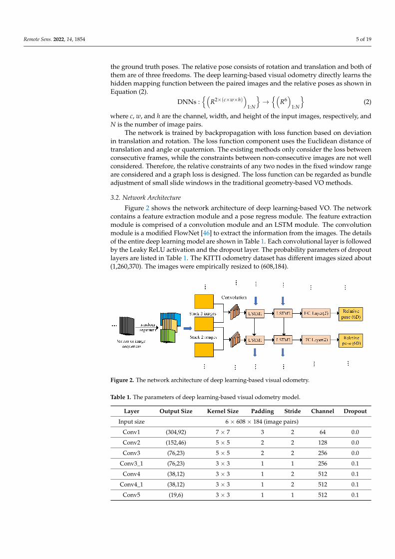
Figure 2 shows the network architecture of deep learning-based VO. The networkcontains a feature extraction module and a pose regress module. The feature extractionmodule is comprised of a convolution module and an LSTM module. The convolutionmodule is a modified FlowNet [46] to extract the information from the images. The detailsof the entire deep learning model are shown in Table 1. Each convolutional layer is followedby the Leaky ReLU activation and the dropout layer. The probability parameters of dropoutlayers are listed in Table 1. The KITTI odometry dataset has different images sized about(1,260,370). The images were empirically resized to (608,184).

Figure 2. The network architecture of deep learning-based visual odometry.

Table 1. The parameters of deep learning-based visual odometry model.

Layer Output Size Kernel Size Padding Stride Channel Dropout

Input size 6 × 608 × 184 (image pairs)

Conv1 (304,92) 7 × 7 3 2 64 0.0

Conv2 (152,46) 5 × 5 2 2 128 0.0

Conv3 (76,23) 5 × 5 2 2 256 0.0

Conv3_1 (76,23) 3 × 3 1 1 256 0.1

Conv4 (38,12) 3 × 3 1 2 512 0.1

Conv4_1 (38,12) 3 × 3 1 2 512 0.1

Conv5 (19,6) 3 × 3 1 1 512 0.1

Remote Sens. 2022, 14, 1854 6 of 19

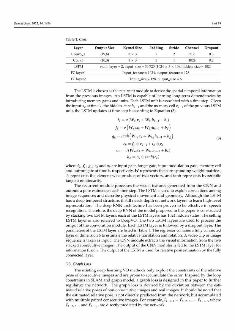
Table 1. Cont.

Layer Output Size Kernel Size Padding Stride Channel Dropout

Conv5_1 (19,6) 3 × 3 1 2 512 0.3

Conv6 (10,3) 3 × 3 1 1 1024 0.2

LSTM num_layer = 2, input_size = 30,720 (1024 × 3 × 10), hidden_size = 1024

FC layer1 Input_feature = 1024, output_feature = 128

FC layer2 Input_size = 128, output_size = 6

The LSTM is chosen as the recurrent module to derive the spatial-temporal informationfrom the previous images. An LSTM is capable of learning long-term dependencies byintroducing memory gates and units. Each LSTM unit is associated with a time step. Giventhe input xk at time k, the hidden state hk−1 and the memory cell ck−1 of the previous LSTMunit, the LSTM updates at time step k according to Equation (3).

ik = σ(Wxixk + Whihk−1 + bi)

fk = σ(

Wx f xk + Wh f hk−1 + b f

)gk = tanh

(Wxgxk + Whghk−1 + bg

)ck = fk � ck−1 + ik � gk

ok = σ(Wxoxk + Whohk−1 + bo)

hk = ok � tanh(ck)

(3)

where ik, fk, gk, ck and ok are input gate, forget gate, input modulation gate, memory celland output gate at time k, respectively, W represents the corresponding weight matrices,� represents the element-wise product of two vectors, and tanh represents hyperbolictangent nonlinearity.

The recurrent module processes the visual features generated from the CNN andoutputs a pose estimate at each time step. The LSTM is used to exploit correlations amongimage sequences and describe physical movement and geometry. Although the LSTMhas a deep temporal structure, it still needs depth on network layers to learn high-levelrepresentation. The deep RNN architecture has been proven to be effective in speechrecognition. Therefore, the deep RNN of the model proposed in this paper is constructedby stacking two LSTM layers; each of the LSTM layers has 1024 hidden states. The settingLSTM layer is also referred to DeepVO. The two LSTM layers are used to process theoutput of the convolution module. Each LSTM layer is followed by a dropout layer. Theparameters of the LSTM layer are listed in Table 1. The regressor contains a fully connectedlayer of dimension 6 to estimate the relative translation and rotation. A video clip or imagesequence is taken as input. The CNN module extracts the visual information from the twostacked consecutive images. The output of the CNN modules is fed to the LSTM layer forinformation fusion. The output of the LSTM is used for relative pose estimation by the fullyconnected layer.

3.3. Graph Loss

The existing deep learning VO methods only exploit the constraints of the relativepose of consecutive images and are prone to accumulate the error. Inspired by the loopconstraints in SLAM and graph model, a graph loss is designed in this paper to furtherregularize the network. The graph loss is devised by the deviation between the esti-mated relative poses of non-consecutive images and real images. It should be noted thatthe estimated relative pose is not directly predicted from the network, but accumulatedwith multiple paired consecutive images. For example, P̂t−2, t = P̂t−2, t−1 · P̂t−1, t, whereP̂t−2, t−1 and P̂t−1, t are directly predicted by the network.

Remote Sens. 2022, 14, 1854 7 of 19

Figure 3 shows the computation of graph loss. To construct the graph, a window isused to slide over the image sequences. Firstly, the image sequences were fed into themodel to predict the relative pose. Then the relative pose was used to calculate the absolutepose. Empirically, the window size was set to 15–20 images to improve the efficiency.For each window, a random strategy was selected to construct the edges of a graph andgenerate more relative edges from the absolute poses. For each iteration edges equal tofour times the window size were randomly selected to further increase the efficiency. Therandom strategy can prevent the network from overfitting compared with using fixededges. The graph loss leads to more edge constraints, which incur some computationalcosts. The computational cost of the loss component is still small compared to the totalnetwork computation.

Figure 3. Computation of graph loss.

For each edge, the relative pose of the model prediction is accumulated into theabsolute pose in a sliding window. The loss function is designed as:

L =1

Ne∑eij∈Epose

d(ζij, ζ̂ij

)(4)

E ={

eij | 1 ≤ |i− j |< windows_size}

(5)

d(ζij, ζ̂ij

)= argmin

(‖t̂ij − tij‖

22 + k ∗ geodesic_rotation_loss(rij, r̂ij)

)(6)

where ζij = (tij, rij) and ζ̂ij =(t̂ij, r̂ij

)are the ground-truth and the predicted value,

respectively. tij and rij denote the translation vector and the rotation vector from frame j toframe i, respectively. d(ζij, ζ̂ij) is the geometric loss function adopted to balance the positionand rotation errors. k is a scale factor to balance the weights of translation and rotation, kwas set to 100 in the experiment.

3.4. Geodesic Rotation Loss

Usually, the traditional rotation loss is designed based on the Euclidean distance ofthe quaternion [7,50], or Euler angle [51–53] between the prediction and the ground truth.It provides a direct difference between the prediction and the ground truth. The Eulerangle and the quaternion themselves are constrained vectors. Using them as optimizationvariables introduces additional constraints on numerical computation making the opti-mization difficult. This leads the network to converge unstably and makes the networkhard to train. Through the transformation relationship between Lie group and Lie algebra,the pose estimation is turned into an unconstrained optimization problem. The geodesicrotation loss is designed to obtain the angle difference on 3D manifold.

Geodesic distance is the appropriate geometric distance that corresponds to the lengthof the shortest path along the manifold [54]. It allows a robust and stable convergence byregressing a Lie algebra so(3): rij. Especially, the Lie algebra so(3) (rij, the output of model)is then converted into Lie group SO(3) according to Equation (7). This is known as theexponential map, an application from so(3) to SO(3). SO(3) is the result of the exponential

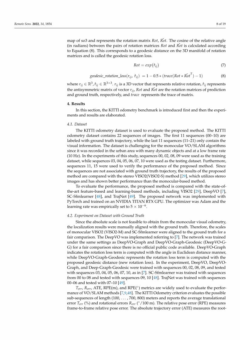
Remote Sens. 2022, 14, 1854 8 of 19

map of so3 and represents the rotation matrix Rot, ˆRot. The cosine of the relative angle(in radians) between the pairs of rotation matrices Rot and ˆRot is calculated accordingto Equation (8). This corresponds to a geodesic distance on the 3D manifold of rotationmatrices and is called the geodesic rotation loss.

Rot = exp(r̂ij)

(7)

geodesic_rotation_loss(rij, r̂ij) = 1− 0.5 ∗ (trace(Rot ∗ ˆRotT)− 1) (8)

where rij ∈ R3, r̂ij ∈ R3×3. rij is a 3D vector that represents relative rotation, r̂ij representsthe antisymmetric matrix of vector rij, Rot and ˆRot are the rotation matrices of predictionand ground truth, respectively, and trace represents the trace of matrix.

4. Results

In this section, the KITTI odometry benchmark is introduced first and then the experi-ments and results are elaborated.

4.1. Dataset

The KITTI odometry dataset is used to evaluate the proposed method. The KITTIodometry dataset contains 22 sequences of images. The first 11 sequences (00–10) arelabeled with ground truth trajectory, while the last 11 sequences (11–21) only contain thevisual information. The dataset is challenging for the monocular VO/SLAM algorithmssince it was recorded in the urban area with many dynamic objects and at a low frame rate(10 Hz). In the experiments of this study, sequences 00, 02, 08, 09 were used as the trainingdataset, while sequences 03, 04, 05, 06, 07, 10 were used as the testing dataset. Furthermore,sequences 11, 15 were used to verify the performance of the proposed method. Sincethe sequences are not associated with ground truth trajectory, the results of the proposedmethod are compared with the stereo VISO2(VISO2-S) method [29], which utilizes stereoimages and has shown better performance than the monocular-based method.

To evaluate the performance, the proposed method is compared with the state-of-the-art feature-based and learning-based methods, including VISO2 [29], DeepVO [7],SC-Sfmlearner [48], and TrajNet [49]. The proposed network was implemented withPyTorch and trained on an NVIDIA TITAN RTX GPU. The optimizer was Adam and thelearning rate was empirically set to 5 × 10−6.

4.2. Experiment on Dataset with Ground Truth

Since the absolute scale is not feasible to obtain from the monocular visual odometry,the localization results were manually aligned with the ground truth. Therefore, the scalesof monocular VISO2 (VISO2-M) and SC-Sfmlearner were aligned to the ground truth for afair comparison. The DeepVO was implemented referring to [7]. The network was trainedunder the same settings as DeepVO-Graph and DeepVO-Graph-Geodesic (DeepVO-G-G) for a fair comparison since there is no official public code available. DeepVO-Graphindicates the rotation loss term is computed with the angle in Euclidean distance manner,while DeepVO-Graph-Geodesic represents the rotation loss term is computed with theproposed geodesic distance (new rotation loss). In the experiment, DeepVO, DeepVO-Graph, and Deep-Graph-Geodesic were trained with sequences 00, 02, 08, 09, and testedwith sequences 03, 04, 05, 06, 07, 10, as in [7]. SC-Sfmlearner was trained with sequencesfrom 00 to 08 and tested with sequences 09, 10 [48]. TrajNet was trained with sequences00–06 and tested with 07–10 [49].

Terr, Rerr, ATE, RPE(m), and RPE(◦) metrics are widely used to evaluate the perfor-mance of VO/SLAM methods [7,9,48]. The KITTI Odometry criterion evaluates the possiblesub-sequences of length (100, . . . , 700, 800) meters and reports the average translationalerror Terr (%) and rotational errors Rerr (◦/100 m). The relative pose error (RPE) measuresframe-to-frame relative pose error. The absolute trajectory error (ATE) measures the root-

Remote Sens. 2022, 14, 1854 9 of 19

mean-square error between the translation of predicted camera poses and ground truth.The RPE and ATE are computed as Equations (9)–(12).

Ei =(

Q−1i Qi+∆

)−1(P−1

i Pi+∆

)(9)

RMSE(E1:n, ∆) =(

1m∑m

i=1‖trans(Ei)‖2) 1

2(10)

RPE =1n∑m

∆=1RMSE(E1:n, ∆) (11)

Fi = Q−1i Pi (12)

ATE =

(1m∑m

i=1‖trans(Fi)‖2) 1

2(13)

where P, Q ∈ SE(3), P and Q represent the predicted and the ground truth poses, respec-tively. ∆ represents the time interval. trans(Ei) can be replaced by rots (Ei). trans(Ei) androts (Ei) represent the translation and the rotation parts of Ei, respectively.

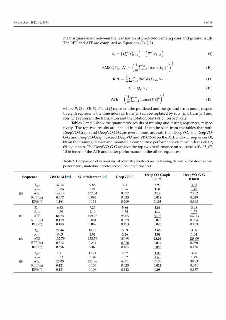
Tables 2 and 3 show the quantitative results of training and testing sequences, respec-tively. The top two results are labeled in bold. It can be seen from the tables that bothDeepVO-Graph and DeepVO-G-G are overall more accurate than DeepVO. The DeepVO-G-G and DeepVO-Graph exceed DeepVO and VISO2-M on the ATE index of sequences 00,08 on the training dataset and maintain a competitive performance on most indexes on 02,09 sequences. The DeepVO-G-G achieve the top two performance on sequences 03, 05, 07,10 in terms of the ATE and better performance on the other sequences.

Table 2. Comparison of various visual odometry methods on the training dataset. (Bold denotes bestperformance, underline denotes second best performance).

Sequence VISO2-M [29] SC-Sfmlearner [48] DeepVO [7] DeepVO-Graph(Ours)

DeepVO-G-G(Ours)

00

Terr 37.14 9.88 4.1 2.99 3.35Rerr 15.84 3.91 1.76 1.37 1.43ATE 142.14 137.34 83.77 31.8 73.02

RPE(m) 0.377 0.093 0.023 0.018 0.029RPE(◦) 1.161 0.134 0.209 0.105 0.198

02

Terr 6.38 7.27 5.86 3.86 3.98Rerr 1.39 2.19 1.75 1.34 1.37ATE 86.73 199.27 95.05 86.98 147.13

RPE(m) 0.119 0.081 0.029 0.023 0.034RPE(◦) 0.183 0.089 0.173 0.093 0.163

08

Terr 24.46 18.26 5.59 2.65 3.38Rerr 8.03 2.01 2.26 1.08 1.54ATE 132.79 133.79 180.91 28.09 128.09

RPE(m) 0.312 0.244 0.026 0.019 0.030RPE(◦) 0.896 0.07 0.164 0.086 0.156

09

Terr 4.41 11.24 4.32 4.04 3.36Rerr 1.23 3.34 1.52 1.49 1.29ATE 18.03 121.96 43.71 37.89 38.83

RPE(m) 0.121 0.106 0.025 0.022 0.031RPE(◦) 0.121 0.106 0.142 0.08 0.137

Remote Sens. 2022, 14, 1854 10 of 19

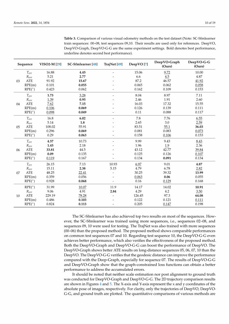
Table 3. Comparison of various visual odometry methods on the test dataset (Note: SC-Sfmlearnertrain sequences: 00–08, test sequences 09,10. Their results are used only for references. DeepVO,DeepVO-Graph, DeepVO-G-G are the same experiment settings. Bold denotes best performance,underline denotes second best performance).

Sequence VISO2-M [29] SC-Sfmlearner [48] TrajNet [49] DeepVO [7] DeepVO-Graph(Ours)

DeepVO-G-G(Ours)

03

Terr 16.88 4.45 - 15.06 9.72 10.00Rerr 5.21 2.77 - 6.6 4.5 4.87ATE 91.92 15.67 - 87.2 46.57 41.92

RPE(m) 0.101 0.055 - 0.065 0.062 0.058RPE(◦) 0.423 0.062 - 0.162 0.109 0.153

04

Terr 1.73 3.28 - 8.04 8.97 7.11Rerr 1.39 0.95 - 2.46 1.91 2.60ATE 7.62 7.15 - 16.03 17.32 15.55

RPE(m) 0.106 0.069 - 0.126 0.139 0.111RPE(◦) 0.098 0.049 - 0.11 0.088 0.117

05

Terr 16.8 6.02 - 7.8 7.76 6.55Rerr 5.14 1.8 - 2.65 3.0 2.59ATE 108.02 55.91 - 83.51 55.1 36.03

RPE(m) 0.296 0.069 - 0.081 0.083 0.073RPE(◦) 0.29 0.063 - 0.158 0.106 0.153

06

Terr 4.57 10.73 - 9.99 9.43 8.43Rerr 1.45 2.18 - 1.96 1.9 2.36ATE 33.81 44.5 - 43.12 42.77 39.84

RPE(m) 0.09 0.135 - 0.125 0.126 0.107RPE(◦) 0.119 0.167 - 0.134 0.091 0.134

07

Terr 26.15 7.13 10.93 6.97 9.01 4.87Rerr 15.11 2.38 5.15 4.79 6.78 2.82ATE 48.25 22.41 - 30.25 39.32 13.99

RPE(m) 0.359 0.056 - 0.063 0.06 0.055RPE(◦) 0.928 0.068 - 0.16 0.129 0.168

10

RPE(◦) 31.99 10.07 11.9 14.17 14.02 10.91Rerr 9.06 4.91 2.84 4.29 4.2 3.50ATE 229.19 78.28 - 126.45 97.3 64.08

RPE(m) 0.486 0.103 - 0.122 0.121 0.111RPE(◦) 0.824 0.113 - 0.205 0.147 0.198

The SC-Sfmlearner has also achieved top two results on most of the sequences. How-ever, the SC-Sfmlearner was trained using more sequences, i.e., sequences 02–08, andsequences 09, 10 were used for testing. The TrajNet was also trained with more sequences(00–06) than the proposed method. The proposed method shows comparable performanceson common test sequences 07 and 10. Regarding test sequence 10, the DeepVO-G-G evenachieves better performance, which also verifies the effectiveness of the proposed method.Both the DeepVO-Graph and DeepVO-G-G can boost the performance of DeepVO. TheDeepVO-Graph shows better ATE results on long-distance sequences 05, 06, 07, 10 than theDeepVO. The DeepVO-G-G verifies that the geodesic distance can improve the performancecompared with the Deep-Graph, especially for sequence 07. The results of DeepVO-G-Gand DeepVO-Graph show that the graph-constrained loss functions can obtain a betterperformance to address the accumulated errors.

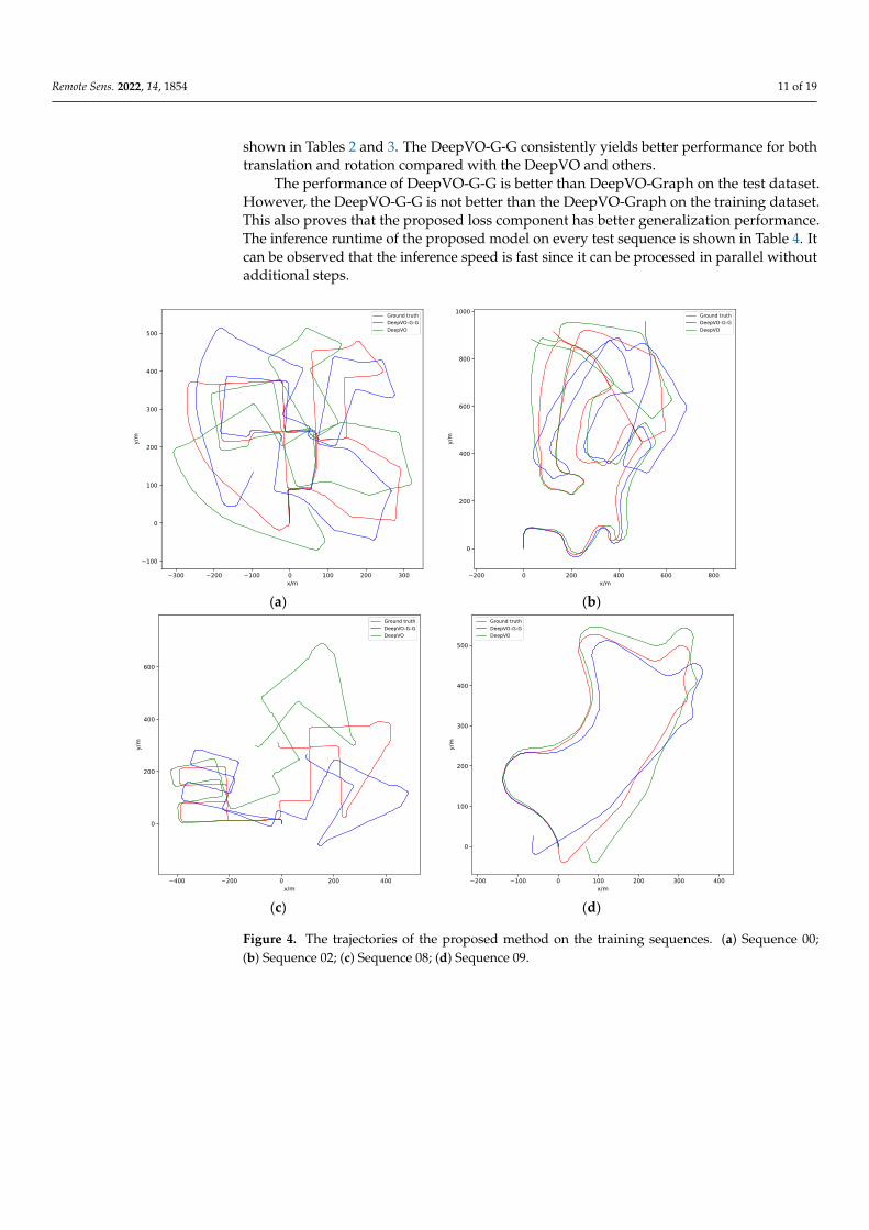
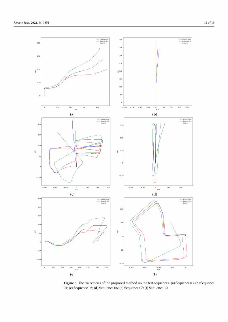
It should be noted that neither scale estimation nor post alignment to ground truthwas conducted for DeepVO-Graph and DeepVO-G-G. The 2D trajectory comparison resultsare shown in Figures 4 and 5. The X-axis and Y-axis represent the x and y coordinates of theabsolute pose of images, respectively. For clarity, only the trajectories of DeepVO, DeepVO-G-G, and ground truth are plotted. The quantitative comparisons of various methods are

Remote Sens. 2022, 14, 1854 11 of 19

shown in Tables 2 and 3. The DeepVO-G-G consistently yields better performance for bothtranslation and rotation compared with the DeepVO and others.

The performance of DeepVO-G-G is better than DeepVO-Graph on the test dataset.However, the DeepVO-G-G is not better than the DeepVO-Graph on the training dataset.This also proves that the proposed loss component has better generalization performance.The inference runtime of the proposed model on every test sequence is shown in Table 4. Itcan be observed that the inference speed is fast since it can be processed in parallel withoutadditional steps.

Remote Sens. 2022, 14, x FOR PEER REVIEW 11 of 19

quences 05, 06, 07, 10 than the DeepVO. The DeepVO-G-G verifies that the geodesic dis-

tance can improve the performance compared with the Deep-Graph, especially for se-

quence 07. The results of DeepVO-G-G and DeepVO-Graph show that the

graph-constrained loss functions can obtain a better performance to address the accu-

mulated errors.

It should be noted that neither scale estimation nor post alignment to ground truth

was conducted for DeepVO-Graph and DeepVO-G-G. The 2D trajectory comparison re-

sults are shown in Figures 4 and 5. The X-axis and Y-axis represent the x and y coordi-

nates of the absolute pose of images, respectively. For clarity, only the trajectories of

DeepVO, DeepVO-G-G, and ground truth are plotted. The quantitative comparisons of

various methods are shown in Tables 2 and 3. The DeepVO-G-G consistently yields better

performance for both translation and rotation compared with the DeepVO and others.

The performance of DeepVO-G-G is better than DeepVO-Graph on the test dataset.

However, the DeepVO-G-G is not better than the DeepVO-Graph on the training da-

taset. This also proves that the proposed loss component has better generalization per-

formance. The inference runtime of the proposed model on every test sequence is shown

in Table 4. It can be observed that the inference speed is fast since it can be processed in

parallel without additional steps.

(a) (b)

(c) (d)

Figure 4. The trajectories of the proposed method on the training sequences. (a) Sequence 00; (b)

Sequence 02; (c) Sequence 08; (d) Sequence 09. Figure 4. The trajectories of the proposed method on the training sequences. (a) Sequence 00;(b) Sequence 02; (c) Sequence 08; (d) Sequence 09.

Remote Sens. 2022, 14, 1854 12 of 19Remote Sens. 2022, 14, x FOR PEER REVIEW 12 of 19

(a) (b)

(c) (d)

(e) (f)

Figure 5. The trajectories of the proposed method on the test sequences. (a) Sequence 03; (b) Se-

quence 04; (c) Sequence 05; (d) Sequence 06; (e) Sequence 07; (f) Sequence 10. Figure 5. The trajectories of the proposed method on the test sequences. (a) Sequence 03; (b) Sequence04; (c) Sequence 05; (d) Sequence 06; (e) Sequence 07; (f) Sequence 10.

Remote Sens. 2022, 14, 1854 13 of 19

Table 4. The inference runtime of the proposed model for different sequences (experiment environ-ment: Ubuntu 18.04, PyTorch Library, Intel Xeon Gold 5222 CPU, RAM 64G, NVIDIA Titan RTXGPU 24G).

Sequence Number of Frames Inference Runtime (s)

03 801 4.604 271 3.605 2761 7.706 1101 4.207 1101 4.210 1201 4.3

4.3. Experiment on Dataset without Ground Truth

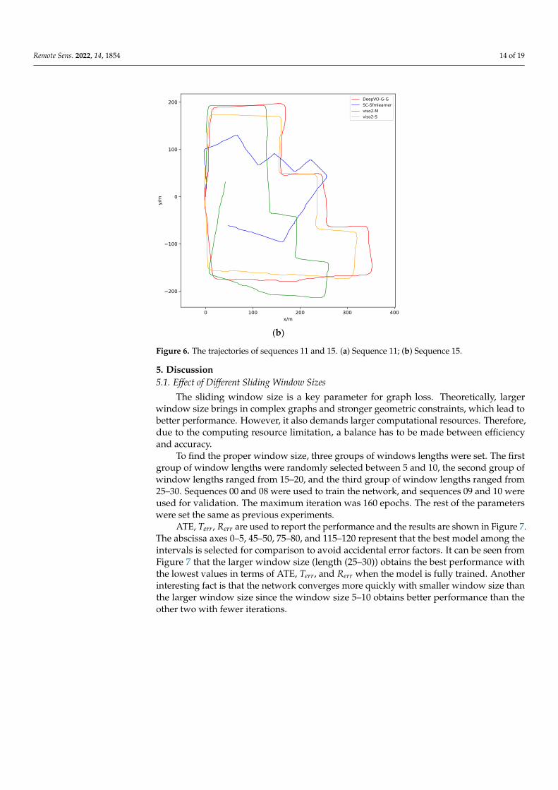
To evaluate the performance of the proposed method, it was tested on test sequences11, 15 using the former experiment model. Since no ground truth trajectory is provided,only the qualitative analysis is performed by generating the trajectory. The VISO2-S ischosen as the ground truth since its effectiveness has been accepted. The proposed methodis also compared with SC-Sfmlearner, DeepVO-G-G, and VISO2-M.

The scale of VISO2-M and SC-Sfmlearner is obtained by aligning to the VISO2-S.The results are shown in Figure 6. The DeepVO-G-G and VISO2-M perform better insequence 11; the SC-Sfmlearner is poorer than the others. Sequence 15 is more challeng-ing (longer distances and scene complexity) than sequence 11. However, the proposedmethod is closer to the VISO2-S than VISO2-M and SC-Sfmlearner on sequence 15, whichdemonstrates that the proposed method achieves better performance than the traditionalmonocular visual odometry and other deep learning-based methods.

Remote Sens. 2022, 14, x FOR PEER REVIEW 13 of 19

Table 4. The inference runtime of the proposed model for different sequences (experiment envi-

ronment: Ubuntu 18.04, PyTorch Library, Intel Xeon Gold 5222 CPU, RAM 64G, NVIDIA Titan

RTX GPU 24G).

Sequence Number of Frames Inference Runtime (sec)

03 801 4.6

04 271 3.6

05 2761 7.7

06 1101 4.2

07 1101 4.2

10 1201 4.3

4.3. Experiment on Dataset without Ground Truth

To evaluate the performance of the proposed method, it was tested on test se-

quences 11, 15 using the former experiment model. Since no ground truth trajectory is

provided, only the qualitative analysis is performed by generating the trajectory. The

VISO2-S is chosen as the ground truth since its effectiveness has been accepted. The

proposed method is also compared with SC-Sfmlearner, DeepVO-G-G, and VISO2-M.

The scale of VISO2-M and SC-Sfmlearner is obtained by aligning to the VISO2-S.

The results are shown in Figure 6. The DeepVO-G-G and VISO2-M perform better in

sequence 11; the SC-Sfmlearner is poorer than the others. Sequence 15 is more challeng-

ing (longer distances and scene complexity) than sequence 11. However, the proposed

method is closer to the VISO2-S than VISO2-M and SC-Sfmlearner on sequence 15,

which demonstrates that the proposed method achieves better performance than the

traditional monocular visual odometry and other deep learning-based methods.

(a)

Figure 6. Cont.

Remote Sens. 2022, 14, 1854 14 of 19Remote Sens. 2022, 14, x FOR PEER REVIEW 14 of 19

(b)

Figure 6. The trajectories of sequences 11 and 15. (a) Sequence 11; (b) Sequence 15.

5. Discussion

5.1. Effect of Different Sliding Window Sizes

The sliding window size is a key parameter for graph loss. Theoretically, larger

window size brings in complex graphs and stronger geometric constraints, which lead to

better performance. However, it also demands larger computational resources. There-

fore, due to the computing resource limitation, a balance has to be made between effi-

ciency and accuracy.

To find the proper window size, three groups of windows lengths were set. The

first group of window lengths were randomly selected between 5 and 10, the second

group of window lengths ranged from 15–20, and the third group of window lengths

ranged from 25–30. Sequences 00 and 08 were used to train the network, and sequences

09 and 10 were used for validation. The maximum iteration was 160 epochs. The rest of

the parameters were set the same as previous experiments.

ATE, 𝑇𝑒𝑟𝑟 , 𝑅𝑒𝑟𝑟 are used to report the performance and the results are shown in

Figure 7. The abscissa axes 0–5, 45–50, 75–80, and 115–120 represent that the best model

among the intervals is selected for comparison to avoid accidental error factors. It can be

seen from Figure 7 that the larger window size (length (25–30)) obtains the best perfor-

mance with the lowest values in terms of ATE, 𝑇𝑒𝑟𝑟 , and 𝑅𝑒𝑟𝑟 when the model is fully

trained. Another interesting fact is that the network converges more quickly with small-

er window size than the larger window size since the window size 5–10 obtains better

performance than the other two with fewer iterations.

Figure 6. The trajectories of sequences 11 and 15. (a) Sequence 11; (b) Sequence 15.

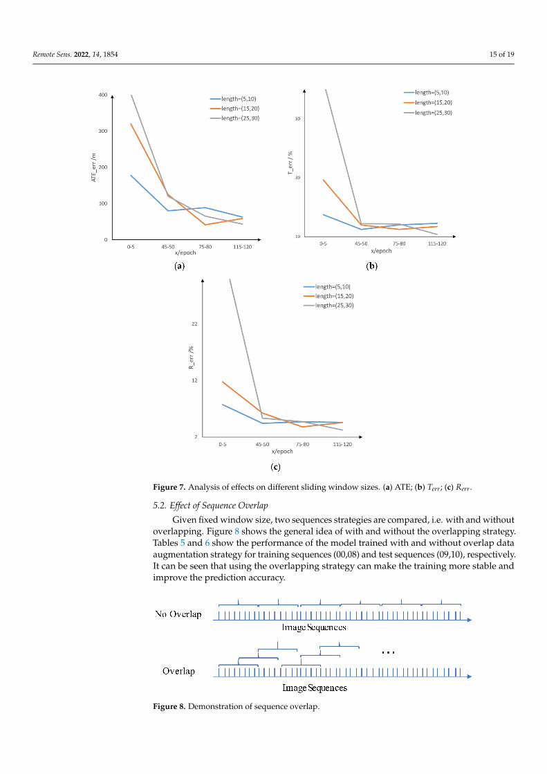
5. Discussion5.1. Effect of Different Sliding Window Sizes

The sliding window size is a key parameter for graph loss. Theoretically, largerwindow size brings in complex graphs and stronger geometric constraints, which lead tobetter performance. However, it also demands larger computational resources. Therefore,due to the computing resource limitation, a balance has to be made between efficiencyand accuracy.

To find the proper window size, three groups of windows lengths were set. The firstgroup of window lengths were randomly selected between 5 and 10, the second group ofwindow lengths ranged from 15–20, and the third group of window lengths ranged from25–30. Sequences 00 and 08 were used to train the network, and sequences 09 and 10 wereused for validation. The maximum iteration was 160 epochs. The rest of the parameterswere set the same as previous experiments.

ATE, Terr, Rerr are used to report the performance and the results are shown in Figure 7.The abscissa axes 0–5, 45–50, 75–80, and 115–120 represent that the best model among theintervals is selected for comparison to avoid accidental error factors. It can be seen fromFigure 7 that the larger window size (length (25–30)) obtains the best performance withthe lowest values in terms of ATE, Terr, and Rerr when the model is fully trained. Anotherinteresting fact is that the network converges more quickly with smaller window size thanthe larger window size since the window size 5–10 obtains better performance than theother two with fewer iterations.

Remote Sens. 2022, 14, 1854 15 of 19

Figure 7. Analysis of effects on different sliding window sizes. (a) ATE; (b) Terr; (c) Rerr.

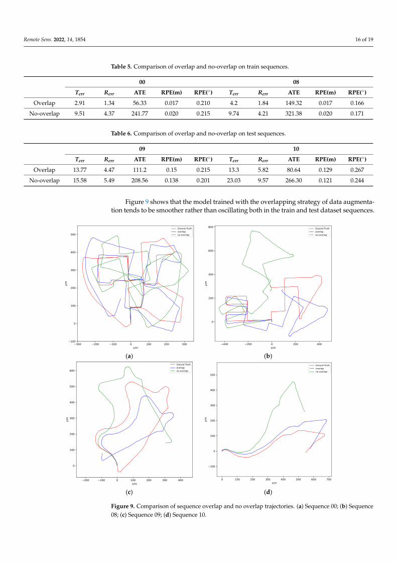
5.2. Effect of Sequence Overlap

Given fixed window size, two sequences strategies are compared, i.e. with and withoutoverlapping. Figure 8 shows the general idea of with and without the overlapping strategy.Tables 5 and 6 show the performance of the model trained with and without overlap dataaugmentation strategy for training sequences (00,08) and test sequences (09,10), respectively.It can be seen that using the overlapping strategy can make the training more stable andimprove the prediction accuracy.

Figure 8. Demonstration of sequence overlap.

Remote Sens. 2022, 14, 1854 16 of 19

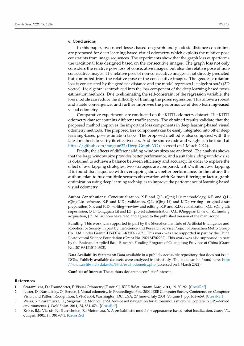
Table 5. Comparison of overlap and no-overlap on train sequences.

00 08

Terr Rerr ATE RPE(m) RPE(◦) Terr Rerr ATE RPE(m) RPE(◦)

Overlap 2.91 1.34 56.33 0.017 0.210 4.2 1.84 149.32 0.017 0.166

No-overlap 9.51 4.37 241.77 0.020 0.215 9.74 4.21 321.38 0.020 0.171

Table 6. Comparison of overlap and no-overlap on test sequences.

09 10

Terr Rerr ATE RPE(m) RPE(◦) Terr Rerr ATE RPE(m) RPE(◦)

Overlap 13.77 4.47 111.2 0.15 0.215 13.3 5.82 80.64 0.129 0.267

No-overlap 15.58 5.49 208.56 0.138 0.201 23.03 9.57 266.30 0.121 0.244

Figure 9 shows that the model trained with the overlapping strategy of data augmenta-tion tends to be smoother rather than oscillating both in the train and test dataset sequences.

Remote Sens. 2022, 14, x FOR PEER REVIEW 16 of 19

Table 5. Comparison of overlap and no-overlap on train sequences.

00 08

𝑻𝒆𝒓𝒓 𝑹𝒆𝒓𝒓 ATE RPE(m) RPE(°) 𝑻𝒆𝒓𝒓 𝑹𝒆𝒓𝒓 ATE RPE(m) RPE(°)

Overlap 2.91 1.34 56.33 0.017 0.210 4.2 1.84 149.32 0.017 0.166

No-overlap 9.51 4.37 241.77 0.020 0.215 9.74 4.21 321.38 0.020 0.171

Table 6. Comparison of overlap and no-overlap on test sequences.

09 10

𝑻𝒆𝒓𝒓 𝑹𝒆𝒓𝒓 ATE RPE(m) RPE(°) 𝑻𝒆𝒓𝒓 𝑹𝒆𝒓𝒓 ATE RPE(m) RPE(°)

Overlap 13.77 4.47 111.2 0.15 0.215 13.3 5.82 80.64 0.129 0.267

No-overlap 15.58 5.49 208.56 0.138 0.201 23.03 9.57 266.30 0.121 0.244

Figure 9 shows that the model trained with the overlapping strategy of data aug-

mentation tends to be smoother rather than oscillating both in the train and test dataset

sequences.

(a) (b)

(c) (d)

Figure 9. Comparison of sequence overlap and no overlap trajectories. (a) Sequence 00; (b) Se-

quence 08; (c) Sequence 09; (d) Sequence 10. Figure 9. Comparison of sequence overlap and no overlap trajectories. (a) Sequence 00; (b) Sequence08; (c) Sequence 09; (d) Sequence 10.

Remote Sens. 2022, 14, 1854 17 of 19

6. Conclusions

In this paper, two novel losses based on graph and geodesic distance constraintsare proposed for deep learning-based visual odometry, which exploits the relative poseconstraints from image sequences. The experiments show that the graph loss outperformsthe traditional loss designed based on the consecutive images. The graph loss not onlyconsiders the relative pose loss of consecutive images, but also the relative pose of non-consecutive images. The relative pose of non-consecutive images is not directly predictedbut computed from the relative pose of the consecutive images. The geodesic rotationloss is constructed by the geodesic distance and the model regresses Lie algebra so(3) (3Dvector). Lie algebra is introduced into the loss component of the deep learning-based posesestimation methods. Due to eliminating the self-constraint of the regression variable, theloss module can reduce the difficulty of training the poses regression. This allows a robustand stable convergence, and further improves the performance of deep learning-basedvisual odometry.

Comparative experiments are conducted on the KITTI odometry dataset. The KITTIodometry dataset contains different traffic scenes. The obtained results validate that theproposed method improves the important loss components in deep learning-based visualodometry methods. The proposed loss components can be easily integrated into other deeplearning-based pose estimation tasks. The proposed method is also compared with thelatest methods to verify its effectiveness. And the source code and weight can be found athttps://github.com/fangxu622/Deep-Graph-VO (accessed on 1 March 2022).

Finally, the effects of different sliding window sizes are analyzed. The analysis showsthat the large window size provides better performance, and a suitable sliding window sizeis obtained to achieve a balance between efficiency and accuracy. In order to explore theeffect of overlapping strategies, two strategies are compared: with/without overlapping.It is found that sequence with overlapping shows better performance. In the future, theauthors plan to fuse multiple sensors observation with Kalman filtering or factor graphoptimization using deep learning techniques to improve the performance of learning-basedvisual odometry.

Author Contributions: Conceptualization, X.F. and Q.L. (Qing Li); methodology, X.F. and Q.L.(Qing Li); software, X.F. and K.D.; validation, Q.L. (Qing Li) and K.D.; writing—original draftpreparation, X.F. and K.D.; writing—review and editing, X.F. and K.D.; visualization, Q.L. (Qing Li);supervision, Q.L. (Qingquan Li) and J.Z.; project administration, Q.L. (Qingquan Li) and J.Z.; fundingacquisition, J.Z. All authors have read and agreed to the published version of the manuscript.

Funding: This work was supported in part by the Shenzhen Institute of Artificial Intelligence andRobotics for Society, in part by the Science and Research Service Project of Shenzhen Metro GroupCo., Ltd. under Grant STJS-DT413-KY002/2021. This work was also supported in part by the ChinaPostdoctoral Science Foundation (Grant No. 2021M702232). This work was also supported in partby the Basic and Applied Basic Research Funding Program of Guangdong Province of China (GrantNo. 2019A1515110303).

Data Availability Statement: Data available in a publicly accessible repository that does not issueDOIs. Publicly available datasets were analyzed in this study. This data can be found here: http://www.cvlibs.net/datasets/kitti/eval_odometry.php (accessed on 1 March 2022).

Conflicts of Interest: The authors declare no conflict of interest.

References1. Scaramuzza, D.; Fraundorfer, F. Visual Odometry [Tutorial]. IEEE Robot. Autom. Mag. 2011, 18, 80–92. [CrossRef]2. Nister, D.; Naroditsky, O.; Bergen, J. Visual odometry. In Proceedings of the 2004 IEEE Computer Society Conference on Computer

Vision and Pattern Recognition, CVPR 2004, Washington, DC, USA, 27 June–2 July 2004; Volume 1, pp. 652–659. [CrossRef]3. Weiss, S.; Scaramuzza, D.; Siegwart, R. Monocular-SLAM–based navigation for autonomous micro helicopters in GPS-denied

environments. J. Field Robot. 2011, 28, 854–874. [CrossRef]4. Kröse, B.J.; Vlassis, N.; Bunschoten, R.; Motomura, Y. A probabilistic model for appearance-based robot localization. Image Vis.

Comput. 2001, 19, 381–391. [CrossRef]

Remote Sens. 2022, 14, 1854 18 of 19

5. Wolf, J.; Burgard, W.; Burkhardt, H. Robust vision-based localization by combining an image-retrieval system with Monte Carlolocalization. IEEE Trans. Robot. 2005, 21, 208–216. [CrossRef]

6. Wiseman, Y. Ancillary ultrasonic rangefinder for autonomous vehicles. Int. J. Secur. Its Appl. 2018, 12, 49–58. [CrossRef]7. Wang, S.; Clark, R.; Wen, H.; Trigoni, N. DeepVO: Towards End-to-End Visual Odometry with Deep Recurrent Convolutional

Neural Networks. In Proceedings of the 2017 IEEE International Conference on Robotics and Automation (ICRA), Singapore,29 May–3 June 2017; pp. 2043–2050. [CrossRef]

8. Saputra, M.R.U.; de Gusmao, P.P.; Wang, S.; Markham, A.; Trigoni, N. Learning monocular visual odometry through geometry-aware curriculum learning. In Proceedings of the 2019 International Conference on Robotics and Automation (ICRA), Montreal,QC, Canada, 20–24 May 2019; pp. 3549–3555.

9. Zhan, H.; Weerasekera, C.S.; Bian, J.-W.; Reid, I. Visual odometry revisited: What should be learnt? In Proceedings of the 2020IEEE International Conference on Robotics and Automation (ICRA), Paris, France, 31 May–31 August 2020; pp. 4203–4210.

10. Clark, R.; Wang, S.; Markham, A.; Trigoni, N.; Wen, H. Vidloc: A deep spatio-temporal model for 6-dof video-clip relocalization.In Proceedings of the IEEE Conference on Computer Vision and Pattern Recognition, Honolulu, HI, USA, 21–26 July 2017;pp. 6856–6864.

11. Li, Q.; Zhu, J.; Cao, R.; Sun, K.; Garibaldi, J.M.; Li, Q.; Liu, B.; Qiu, G. Relative Geometry-Aware Siamese Neural Network for6DOF Camera Relocalization. Neurocomputing 2021, 426, 134–146. [CrossRef]

12. Xue, F.; Wu, X.; Cai, S.; Wang, J. Learning Multi-View Camera Relocalization With Graph Neural Networks. In Proceedingsof the 2020 IEEE/CVF Conference on Computer Vision and Pattern Recognition (CVPR), Seattle, WA, USA, 13–19 June 2020;pp. 11372–11381. [CrossRef]

13. Hochreiter, S.; Schmidhuber, J. Long short-term memory. Neural Comput. 1997, 9, 1735–1780. [CrossRef]14. Zhang, Z. A flexible new technique for camera calibration. IEEE Trans. Pattern Anal. Mach. Intell. 2000, 22, 1330–1334. [CrossRef]15. Kumar, G.; Bhatia, P.K. A detailed review of feature extraction in image processing systems. In Proceedings of the 2014 Fourth

International Conference on Advanced Computing & Communication Technologies, Rohtak, India, 8–9 February 2014; pp. 5–12.16. Kummerle, R.; Grisetti, G.; Strasdat, H.; Konolige, K.; Burgard, W. G2O: A general framework for graph optimization. In Proceed-

ings of the 2011 IEEE International Conference on Robotics and Automation, Shanghai, China, 9–13 May 2011; pp. 3607–3613.[CrossRef]

17. Dellaert, F.; Kaess, M. Factor Graphs for Robot Perception. Found. Trends Robot. 2017, 6, 1–139. [CrossRef]18. Jiang, S.; Jiang, C.; Jiang, W. Efficient structure from motion for large-scale UAV images: A review and a comparison of SfM tools.

ISPRS J. Photogramm. Remote Sens. 2020, 167, 230–251. [CrossRef]19. Ji, S.; Qin, Z.; Shan, J.; Lu, M. Panoramic SLAM from a multiple fisheye camera rig. ISPRS J. Photogramm. Remote Sens. 2020, 159,

169–183. [CrossRef]20. Qin, T.; Li, P.; Shen, S. VINS-Mono: A Robust and Versatile Monocular Visual-Inertial State Estimator. IEEE Trans. Robot. 2018, 34,

1004–1020. [CrossRef]21. Campos, C.; Elvira, R.; Rodriguez, J.J.G.; Montiel, J.M.M.; Tardos, J.D. ORB-SLAM3: An Accurate Open-Source Library for Visual,

Visual–Inertial, and Multimap SLAM. IEEE Trans. Robot. 2021, 37, 1874–1890. [CrossRef]22. Rosinol, A.; Abate, M.; Chang, Y.; Carlone, L. Kimera: An open-source library for real-time metric-semantic localization

and mapping. In Proceedings of the 2020 IEEE International Conference on Robotics and Automation (ICRA), Paris, France,31 May–31 August 2020; pp. 1689–1696.

23. Zhang, G. Towards Optimal 3D Reconstruction and Semantic Mapping. Ph.D. Thesis, University of California, Merced, CA,USA, 2021.

24. Rosten, E.; Drummond, T. Machine learning for high-speed corner detection. In Proceedings of the European Conference onComputer Vision, Graz, Austria, 7–13 May 2006; Springer: Berlin/Heidelberg, Germany, 2006; pp. 430–443.

25. Bay, H.; Ess, A.; Tuytelaars, T.; van Gool, L. Speeded-up robust features (SURF). Comput. Vis. Image Underst. 2008, 110, 346–359.[CrossRef]

26. Calonder, M.; Lepetit, V.; Strecha, C.; Fua, P. Brief: Binary robust independent elementary features. In Proceedings of theEuropean Conference on Computer Vision, Heraklion, Greece, 5–11 September 2010; Springer: Berlin/Heidelberg, Germany,2010; pp. 778–792.

27. Harris, C.; Stephens, M. A combined corner and edge detector. Alvey Vis. Conf. 1988, 15, 10–5244.28. Aguiar, A.; Sousa, A.; Santos, F.N.d.; Oliveira, M. Monocular Visual Odometry Benchmarking and Turn Performance Optimization.

In Proceedings of the 2019 IEEE International Conference on Autonomous Robot Systems and Competitions (ICARSC), Porto,Portugal, 24–26 April 2019; pp. 1–6. [CrossRef]

29. Geiger, A.; Ziegler, J.; Stiller, C. StereoScan: Dense 3d reconstruction in real-time. In Proceedings of the 2011 IEEE IntelligentVehicles Symposium (IV), Baden-Baden, Germany, 5–9 June 2011; pp. 963–968. [CrossRef]

30. Mur-Artal, R.; Tardós, J.D. ORB-SLAM2: An Open-Source SLAM System for Monocular, Stereo, and RGB-D Cameras. IEEE Trans.Robot. 2017, 33, 1255–1262. [CrossRef]

31. Engel, J.; Schöps, T.; Cremers, D. LSD-SLAM: Large-Scale Direct Monocular SLAM. In Proceedings of the Computer Vision—ECCV2014; Fleet, D., Pajdla, T., Schiele, B., Tuytelaars, T., Eds.; Springer International Publishing: Cham, Switzerland, 2014; Volume 8690,pp. 834–849. [CrossRef]

32. Engel, J.; Koltun, V.; Cremers, D. Direct sparse odometry. IEEE Trans. Pattern Anal. Mach. Intell. 2017, 40, 611–625. [CrossRef]

Remote Sens. 2022, 14, 1854 19 of 19

33. Krizhevsky, A.; Sutskever, I.; Hinton, G.E. Imagenet classification with deep convolutional neural networks. Commun. ACM 2017,60, 84–90. [CrossRef]

34. Redmon, J.; Farhadi, A. YOLOv3: An Incremental Improvement. arXiv 2018, arXiv:1804.02767. Available online: http://arxiv.org/abs/1804.02767 (accessed on 21 April 2021).

35. Ren, S.; He, K.; Girshick, R.; Sun, J. Faster R-CNN: Towar ds Real-Time Object Detection with Region Proposal Networks. arXiv2016, arXiv:1506.01497. Available online: http://arxiv.org/abs/1506.01497 (accessed on 19 February 2021). [CrossRef]

36. Kwon, H.; Kim, Y. BlindNet backdoor: Attack on deep neural network using blind watermark. Multimed. Tools Appl. 2022, 81,6217–6234. [CrossRef]

37. Kendall, A.; Cipolla, R. Geometric Loss Functions for Camera Pose Regression With Deep Learning. In Proceedings of the IEEEConference on Computer Vision and Pattern Recognition, Honolulu, HI, USA, 21–26 July 2017.

38. Konda, K.R.; Memisevic, R. Learning visual odometry with a convolutional network. In Proceedings of the VISAPP (1), Berlin,Germany, 11–14 March 2015; pp. 486–490.

39. Vu, T.; van Nguyen, C.; Pham, T.X.; Luu, T.M.; Yoo, C.D. Fast and efficient image quality enhancement via desubpixel convolutionalneural networks. In Proceedings of the European Conference on Computer Vision (ECCV) Workshops, Munich, Germany,8–14 September 2018.

40. Jeon, M.; Jeong, Y.-S. Compact and Accurate Scene Text Detector. Appl. Sci. 2020, 10, 2096. [CrossRef]41. Kendall, A.; Grimes, M.; Cipolla, R. PoseNet: A Convolutional Network for Real-Time 6-DOF Camera Relocalization. In

Proceedings of the 2015 IEEE International Conference on Computer Vision (ICCV), Santiago, Chile, 7–13 December 2015;pp. 2938–2946. [CrossRef]

42. Zhou, L.; Luo, Z.; Shen, T.; Zhang, J.; Zhen, M.; Yao, Y.; Fang, T.; Quan, L. KFNet: Learning Temporal Camera Relocalizationusing Kalman Filtering. In Proceedings of the IEEE/CVF Conference on Computer Vision and Pattern Recognition, Seattle, WA,USA, 13–19 June 2020; pp. 4919–4928.

43. Li, Q.; Zhu, J.; Liu, J.; Cao, R.; Fu, H.; Garibaldi, J.M.; Li, Q.; Lin, B.; Qiu, G. 3D map-guided single indoor image localizationrefinement. ISPRS J. Photogramm. Remote Sens. 2020, 161, 13–26. [CrossRef]

44. Costante, G.; Mancini, M.; Valigi, P.; Ciarfuglia, T.A. Exploring Representation Learning With CNNs for Frame-to-FrameEgo-Motion Estimation. IEEE Robot. Autom. Lett. 2016, 1, 18–25. [CrossRef]

45. Muller, P.; Savakis, A. Flowdometry: An optical flow and deep learning based approach to visual odometry. In Proceedingsof the 2017 IEEE Winter Conference on Applications of Computer Vision (WACV), Santa Rosa, CA, USA, 24–31 March 2017;pp. 624–631.

46. Dosovitskiy, A.; Fischer, P.; Ilg, E.; Hausser, P.; Hazirbas, C.; Golkov, V.; Van Der Smagt, P.; Cremers, D.; Brox, T. Flownet: Learningoptical flow with convolutional networks. In Proceedings of the IEEE International Conference on Computer Vision, Santiago,Chile, 7–13 December 2015; pp. 2758–2766.

47. Wang, S.; Clark, R.; Wen, H.; Trigoni, N. End-to-end, sequence-to-sequence probabilistic visual odometry through deep neuralnetworks. Int. J. Robot. Res. 2018, 37, 513–542. [CrossRef]

48. Bian, J.; Li, Z.; Wang, N.; Zhan, H.; Shen, C.; Cheng, M.M.; Reid, I. Unsupervised scale-consistent depth and ego-motion learningfrom monocular video. Adv. Neural Inf. Process. Syst. 2019, 32, 35–45.

49. Zhao, C.; Tang, Y.; Sun, Q.; Vasilakos, A.V. Deep Direct Visual Odometry. IEEE Trans. Intell. Transp. Syst. 2021, 1–10. [CrossRef]50. Clark, R.; Wang, S.; Wen, H.; Markham, A.; Trigoni, N. VINet: Visual-Inertial Odometry as a Sequence-to-Sequence Learning

Problem. arXiv 2017, arXiv:1701.08376.51. Liu, Q.; Li, R.; Hu, H.; Gu, D. Using Unsupervised Deep Learning Technique for Monocular Visual Odometry. IEEE Access 2019,

7, 18076–18088. [CrossRef]52. Jiao, J.; Jiao, J.; Mo, Y.; Liu, W.; Deng, Z. Magicvo: End-to-end monocular visual odometry through deep bi-directional recurrent

convolutional neural network. arXiv 2018, arXiv:1811.10964.53. Fang, Q.; Hu, T. Euler angles based loss function for camera relocalization with Deep learning. In Proceedings of the 2018 IEEE

8th Annual International Conference on CYBER Technology in Automation, Control, and Intelligent Systems (CYBER), Tianjin,China, 19–23 July 2018.

54. Li, D.; Dunson, D.B. Geodesic Distance Estimation with Spherelets. arXiv 2020, arXiv:1907.00296. Available online: http://arxiv.org/abs/1907.00296 (accessed on 28 January 2022).