Explicit investment rules with time-to-build and uncertainty

Explicit investment rules with time-to-build and uncertainty∗

René Aid† Salvatore Federico‡ Huyên Pham§ Bertrand Villeneuve¶

June 5, 2014

Abstract

We establish explicit socially optimal rules for an irreversible investment deci-sion with time-to-build and uncertainty. Assuming a price sensitive demand functionwith a random intercept, we provide comparative statics and economic interpreta-tions for three models of demand (arithmetic Brownian, geometric Brownian, and theCox-Ingersoll-Ross). Committed capacity, that is, the installed capacity plus the in-vestment in the pipeline, must never drop below the best predictor of future demand,minus two biases. The discounting bias takes into account the fact that investment ispaid upfront for future use; the precautionary bias multiplies a type of risk aversionindex by the local volatility. Relying on the analytical forms, we discuss in detail theeconomic effects.

Keywords: optimal capacity; irreversible investments; singular stochastic control; time-to-build; delay equations.AMS Classification: 93E20, 49J40, 91B38.JEL Classification: C61; D92; E22.

1 IntroductionHow to track demand when the time-to-build retards capacity expansion? When to investand how much? We answer these questions with a model of irreversible investment. Inthis model, the objective of the decision-maker is to minimize the total discounted socialcost. That is, the decision-maker maximizes the standard microeconomic social surplus.We are able to show in particular that the solution is implementable as a competitiveequilibrium. We are able to calculate explicit, compact, decision rules.

In many capitalistic industries, construction delays are essential. In this paper, wefocus on electricity generation. In this sector, construction delays can be considerable:they could be only one year for a small wind-farm but could be three years for a gas turbineand eight to ten years for a nuclear plant. The scenarios of the evolution of demand withtheir trends, their drag force, and their stochastic parts require particular attention. Tothis purpose, we develop the comparative statics and economic interpretations for threedemand models applied to electricity generation. The intercept of the price sensitivedemand function follows either an arithmetic Brownian motion as in Bar-Ilan et al. [2002],or a geometric Brownian motion as in Bar-Ilan and Strange [1996] and Aguerrevere [2003],or the Cox-Ingersoll-Ross (CIR) model. The latter is a mean-reverting process, and, to∗This study was supported by FiME (Laboratoire de Finance des Marchés de l’Energie) and the “Finance

et Développement Durable - Approches Quantitatives” Chair.†EDF R&D and www.fime-lab.org. [email protected]‡Università degli Studi di Milano. [email protected]§LPMA, Université Paris-Diderot. [email protected]¶LEDa, Université Paris-Dauphine. [email protected]

1

arX

iv:1

406.

0055

v1 [

q-fi

n.M

F] 3

1 M

ay 2

014

our knowledge, no real options investment model exists in the literature with time-to-buildand a process of this type. The basic existence and regularity results are provided in acompanion paper (Federico and Pham [2014]), but we simplify the specification for thesake of calculability.

An exact decision rule facilitates the clear understanding of the effects at play. Thedecision rule stipulates what the committed capacity should be, that is, the installedcapacity plus capacity under construction. The action rule, given the current conditions,is that the committed capacity must not fall below the best predictor of demand after thedelay, minus two biases. The first bias is a pure discounting bias unrelated to uncertainty:because the investment is paid for upfront but only produces after the delay, the requiredcommitted capacity is reduced. The second one is a precautionary bias where a riskaversion index is multiplied by local volatility .

Because of this decomposition, we find the following qualitative results. For investmentwith a long construction horizon, we find that uncertainty has very little importancecompared to the trend of demand growth. Thus, an error on the long-term trend is muchmore harmful than an error on volatility. For investment with a short construction horizon,the opposite is true: decision-makers should pay greater attention to volatility. We alsoillustrate the practical importance of a possible saturation of the demand with the CIRmodel. The investors’ behavior is very different depending on whether demand is aboveor below the long-run average, or target. When demand is above the target, the investoris almost insensitive to the current demand, except if the return speed is very slow. Belowthe target, the comparison between the time-to-build and the expected time-to-target iscritical: if the time-to-build is longer, then the optimal committed capacity is practicallythe target itself minus the biases; if the time-to-build is shorter, then the investors observethe process and invest progressively.

The literature on the topic provides a number of insights. Table 1 provides a tentativeclassification. The competitive pressure matters: competition kills the value of waiting andthus accelerates investment. Grenadier [2000, 2002] and Pacheco de Almeida and Zemsky[2003] follow this line of thought. We exclusively use a competitive market and show thatthis effect is completely internalized. The seminal work McDonald and Siegel [1986] on theoption to wait in the case of irreversible decisions shows that uncertainty has a negativeeffect on investment. Strong support for this result is that with greater volatility, invest-ment is triggered by a higher current product price, i.e. a smaller probability of a marketdownturn. Several extensions provide conditions under which this result does not hold ormight be mitigated. Construction delays, that is, the time between the decision and theavailability of the new capacity, have attracted the attention of economists. In particular,the models in Bar-Ilan and Strange [1996], Bar-Ilan et al. [2002], and Aguerrevere [2003]exhibit situations where an increase in uncertainty leads to an increase in investment.

The models that exhibit a positive effect on investment from an increase in uncertainty,do so only for a specific range of parameters. Besides, the quantitative effects are verysmall. Bar-Ilan et al. [2002] show in their simulations that when the uncertainty ondemand is multiplied by five, then the investment threshold moves only by 1%. And asthe authors themselves point out, the investment thresholds are nearly independent of thelevel of uncertainty. The large effects found in Majd and Pindyck [1987] are reconsideredin Milne and Whalley [2000].

In Aguerrevere [2003], a paper with which we share most of the modeling choices, theproduction is flexible, although the capacity accumulation is not. Investors keep the choiceto produce only when it is profitable, and thus the rigidity of investment is attenuated bythe option to produce or not. The capacity reserves are all the more profitable the longerthe time-to-build. In consequence, uncertainty tends to increase the investment rate. Thispaper is significant because of the way it integrates meaningful economic questions, and

2

Paper Objective Competition Investment

Majd and Pindyck 1987 firm no irreversibleBar-Ilan and Strange 1996 firm no reversibleGrenadier 2000 firm perfect irreversibleBar-Ilan et al. 2002 planner no irreversibleGrenadier 2002 firm imperfect irreversibleAguerrevere 2003 planner/firm perfect/imperfect irreversible with

flexible production

Table 1: Papers on investment with uncertainty and time-to-build.

the numerical simulations are instructive.As far as electricity production is concerned, the flexibility of the base production is

limited either for technological reasons (nuclear plants) or because the fixed cost per idleperiod are important (coal- or gas-fired power plants). In which case, the cost differencebetween producing or not is narrow. Our approach fills a gap in the literature.

This paper is organized as follows. Section 2 describes and justifies our modeling ap-proach. Solutions and general properties are provided in Section 3. We give the expressionof the decision rule and we show that the solution to the optimization program can bedecentralized as a competitive equilibrium. The economic analysis of the joint effect oftime-to-build and uncertainty is given in Section 4 for the a geometric Brownian motion,and in Section 5 for the CIR model. Section 6 concludes.

For information on the popular arithmetic Brownian motion application, please seeAppendix A.

2 The modelWe set up a model of an irreversible investment decision in which the objective is to trackthe current demand of electricity as closely as possible.

1. The inverse demand function at date t is

pt(Q) = η + θ(Dt −Q), (1)

with η ≥ 0 and θ > 0, where p is the price and Q is the output.1 The (quasi) intercept(Dt)t≥0 is a diffusion that satisfies the SDE

dDt = µ(Dt)dt+ σ(Dt)dWt,

D0 = d,(2)

where (Wt)t≥0 is a Brownian motion on some filtered probability space (Ω,F , (Ft)t≥0,P).Without loss of generality, we suppose that the filtration (Ft)t≥0 is the one generated bythe Brownian motion W and enlarged by the P-null sets.

2. There is a time lag h > 0 between the date of the investment decision and the datewhen the investment is completed and becomes productive. Thus, the investment decisionat time t brings additional capacity at time t+ h.

1Aguerrevere [2003] takes a similar form and discusses its flexibility.

3

3. At time t = 0, there is an initial stream of pending investments initiated in the interval[−h, 0) that are going to be completed in the interval [0, h). The function that representsthe cumulative investment planned in the interval [−h, s], s ∈ (−h, 0), is a nonnegativenon-decreasing càdlàg function. Therefore, the set where this function lives is

I0 = I0 : [−h, 0)→ R+, s 7→ I0s càdlàg, non-decreasing. (3)

We set

I00− = lim

s↑0I0s , I0 ∈ I0. (4)

4. The decision variable is represented by a càdlàg non-decreasing (Ft)t≥0-adapted pro-cess (It)t≥0 that represents the cumulative investment from time 0 up to time t ≥ 0.Therefore, formally dIt is the investment at time t ≥ 0. The set of admissible strategies,which we denote by I, is the set

I = I : R+ × Ω→ R+, I càdlàg, (Ft)t≥0-adapted, nondecreasing. (5)

5. Due to the considerations above, given I0 ∈ I0, I ∈ I and setting I−h− = 0, weassume that the production capacity (Kt)t≥0 follows the controlled dynamics driven bythe state equation

dKt = dIt−h,K0− = k, Is = I0

s , s ∈ [−h, 0).(6)

The equation above is a controlled locally deterministic differential equation with delay inthe control variable. By solution to this equation, we mean the the càdlàg process:

Kt = k + It−h, ∀t ≥ 0, (7)

where I is the process

It =I0t , t ∈ [−h, 0),I0

0− + It, t ≥ 0.(8)

Significantly, the randomness in (6) enters only through I, and there are no stochasticintegrals.

6. The objective is to minimize over I ∈ I the functional

F (k, d, I0; I) = E[∫ +∞

0e−ρt

(12(Kt −Dt)2dt+ q0dIt

)], (9)

where q0 > 0 is the unit investment cost.

Economic interpretation of the loss function. The program is a maximization ofthe social surplus or conversely the minimization of the deadweight loss. Given (1), theinstantaneous net consumers’ surplus is by standard definition:

St =∫ Kt

0(η + θ(Dt − q)) dq − ptKt. (10)

This is the sum of the values given to each unit consumed minus the price paid for them. Ifthe unit production cost is η and if there is some fixed cost F per year, the instantaneous

4

producer’s profit πt is (pt − η)Kt − F . The total instantaneous surplus TSt = St + πt istherefore:

TSt = θ

∫ Kt

0(Dt − q) dq − F (11)

= −θ2 (Kt −Dt)2︸ ︷︷ ︸Depends on control

+ θ

2D2t − F︸ ︷︷ ︸

Doesn’t

. (12)

Maximizing the discounted social surplus minus the investment costs amounts to program(9), where the true investment cost q0 is divided by θ.

Thus, the solution and (1) generate an electricity price process. It reflects the marginalcost plus a term, which can be negative, that reflects tension in the market.

Diffusion process. The process D satisfies the following conditions:2 we assume thatthe coefficients µ, σ : R → R in (2) are continuous with sublinear growth and regularenough to ensure the existence of a unique strong solution to (2). Further, we assume thatthis solution takes values in an open set O of R and that it is non-degenerate over thisset, that is, σ2 > 0 on O. In the example we shall discuss in the next section, the set Owill be R or (0,+∞). We observe that, due to the assumption of sublinear growth of µ, σ,standard estimates in SDEs (see, e.g., Krylov [1980, Ch. II]) show that there exist κ0, κ1depending on µ, σ such that

E[|Dt|2

]≤ κ0(1 + |d|2)eκ1t, t ≥ 0. (13)

3 SolutionThe problems with delay are by nature of infinite dimension. Referring to our case, thefunctional F defined in (9) depends not only on the initial k but also on the past of thecontrol I0, which is a function. Nevertheless, the problem can be reformulated in terms ofanother one-dimensional state variable not affected by the delay. We rewrite the objectivefunctional to introduce a new state variable, the so-called committed capacity.

The idea of the reformulation in control problems with delay is contained in Bar-Ilanet al. [2002] (cf. also Bruder and Pham [2009]) in the context of optimal stochastic impulseproblems. Here, we develop this idea for singular stochastic control. It is worth stressingthat, unlike Bar-Ilan et al. [2002], we simplify the approach by working not on the valuefunction of the optimization problem but directly on the basic functional.

3.1 Reduction to a problem without delay

For the case of the domain for the couple of variables (k, d) of our problem, the set is:3

S = R×O. (14)

Define the committed capacity as:

Ct := Kt + It − It−h = Kt+h. (15)2A reference for the theory of one-dimensional diffusions is Karatzas and Shreve [1991].3The real problem is meaningful for k ≥ 0; nevertheless, it is convenient from the mathematical point

of view to allow the case of k < 0. Because the problem is irreversible and starts from k ≥ 0, the capitalremains nonnegative.

5

In differential form, the dynamics of Ct isdCt = dIt,C0− = c = k + I0

0− .(16)

Therefore, it does not contain the delay in the control variable.From now on, the dependence of K on k, I0, I; the dependence of C on c, I; and the

dependence of D on d is denoted respectively as Kk,I0,I , Cc,I , and Dd.The crucial facts that allow the removal of the delay are the following.

1. The committed capacity is (Ft)t≥0-adapted. This is due to the special structure ofthe controlled dynamics of K that makes Kk,I0,I

t+h known given the information Ft.

2. Within the interval [0, h), the control I does not affect the dynamics of Kk,I0,I ,which is (deterministic and) fully determined by I0. In other words, Kk,I0,I(1)

t =Kk,I0,I(2)

t for every t ∈ [0, h) and every I(1), I(2) ∈ I. Therefore, we can writewithout ambiguity Kk,I0

t for t ∈ [0, h) to refer to the “controlled” process K withinthe interval [0, h).

Given these observations, we have the following:

Proposition 1.

F (k, d, I0; I) = E[∫ +∞

0e−ρt

(g(Cc,It , Dd

t )dt+ q0dIt)]

+ J(k, d, I0), (17)

where

J(k, d, I0) = 12 E

[∫ h

0e−ρt

(Kk,I0

t −Ddt

)2dt], (18)

and g : S → R+ is defined by

g(c, d) : = 12e−ρhE

[(c−Dd

h)2]

= 12e−ρh(c2 − 2β0(d)c+ α0(d)), (19)

where

α0(d) :=E[∣∣Dd

h

∣∣2], β0(d) := E[Ddh

]. (20)

Proof. Using the definition of g, the time-homogenous property of D, we have:

E[g(Cc,It , Dd

t )]

= 12e−ρhE

[E[(c′ −Dd′

h )2] ∣∣∣c′=Cc,It , d′=Ddt

]= 1

2e−ρhE

[E[(Cc,It −Dd

t+h)2 | Ft]]

= 12e−ρhE

[(Cc,It −Dd

t+h)2]

= 12e−ρhE

[(Kk,I0,I

t+h −Ddt+h)2

]. (21)

6

Therefore, (9) can be rewritten as

F (k, d, I0; I) = E[∫

[0,h)e−ρt

(12(Kk,I0,It −Dd

t

)2dt+ q0dIt

)]

+ E[∫

[h,+∞)e−ρt

(12(Kk,I0,It −Dd

t

)2dt+ q0dIt

)]

= E[∫

[0,h)e−ρt

(12(Kk,I0,It −Dd

t

)2dt+ q0dIt

)]

+ E[∫ +∞

0e−ρ(t+h)

(12(Kk,I0,It+h −Dd

t+h

)2dt+ q0dIt+h

)]= E

[∫ +∞

0e−ρt

(g(Cc,It , Dd

t )dt+ q0dIt)]

+ J(k, d, I0). (22)

Thus, the functional J(k, d, I0) defined in Proposition 1 does not depend on I ∈ I.Therefore, by setting

G(c, d; I) := E[∫ +∞

0e−ρt

(g(Cc,It , Dd

t ) + q0dIt)], (23)

the original optimization problem of minimizing F (k, d, I0; ·) over I is equivalent to theoptimization problem without delay

v(c, d) := infI∈I

G(c, d; I) subject to (16) and (2). (24)

3.2 Solution characterization

In the sequel, to give sense to the problem (i.e., to guarantee finiteness), we make thestanding assumption that the discount factor ρ satisfies

ρ > max(κ1, 0), (25)

where κ1 is the constant appearing in (13). This assumption guarantees that there is someκ depending on µ, σ s.t.

0 ≤ v(c, d) ≤ κ (1 + |c|2 + |d|2), ∀(c, d) ∈ S. (26)

In particular, it implies that the value function v is finite and locally bounded.Federico and Pham [2014] prove the following facts.4

1. v is convex with respect to the variable c

2. v is differentiable with respect to c, and vc is continuous in S

3. The function d 7→ vc(c, d) does not increase for each c ∈ R

4. vc ≥ −q0

4Federico and Pham [2014] deal with reversible problems. We can apply their results by taking aninfinite cost of disinvestment. The irreversible case with a profit maximization criterion is studied withsimilar generality in Ferrari [forth.].

7

In view of these facts, there is now the continuation region

C := (c, d) ∈ S | vc(c, d) > −q0, (27)

and the action region

A := (c, d) ∈ S | vc(c, d) = −q0. (28)

Therefore, C andA are disjoint and S = C∪A. Due to the continuity of vc, the continuationregion is an open set of S, while the action region is a closed set of S. Moreover, due tothe monotonicity of vc(c, ·) and to the convexity of v(·, d), C and A can be rewritten as

C = (c, d) ∈ S | c > c(d), A = (c, d) ∈ S | c ≤ c(d), (29)

where c : O → R is a non-decreasing function. The latter function is the optimal boundaryfor the problem in the sense that it characterizes the optimal control. Thus, in this singularstochastic optimal control, the optimal control consists of keeping the state processeswithin the closure of the continuation region C by reflecting the controlled process on theoptimal boundary along the direction of the control. See Figure 1.

-

d

C

A

6

66

66

6

c(d)c

Figure 1: Continuation region (C) and action region (A) in the demand-committed capac-ity space.

We have an explicit characterization of c, that is, of the optimal control that is providedby the following result.

Theorem 1. The optimal boundary is explicitly written as

c(d) = β0(d)− q0ρeρh + 1

2σ2(d) β

′′(d)ψ′(d)− β′(d)ψ′′(d)ψ′(d) , (30)

where β0(d) is defined in (20) as E[Ddh

],

β(d) :=∫ +∞

0e−ρtE[β0(Dd

t )]dt, (31)

and ψ is the strictly increasing fundamental solution to the linear ODE

[Lφ](d) := ρφ(d)− µ(d)φ′(d)− 12σ

2(d)φ′′(d) = 0, d ∈ O. (32)

The unique optimal control for the problem (24) is the process

I∗t =[c

(sup

0≤s≤tDds

)− c]+

. (33)

8

Proof. Theorem 4.2 and Corollary 5.2 of Federico and Pham [2014] state the above claim5

with

c(d) = ρ

[β(d)− ψ(d)

ψ′(d)β′(d)− q0e

ρh], (34)

Therefore, if (34) can be rewritten in the form (30), then it is more suitable for interpre-tation.

To this purpose, because ψ solves the ODE (32), we have

c(d) = ρβ(d)− µ(d)β′(d)− 12σ

2(d)ψ′′(d)ψ′(d) β

′(d)− q0ρeρh. (35)

On the other hand, it is well-known from the connection between the linear ODE and theone-dimensional diffusions that the function β solves the nonhomogeneous ODE (32) withthe forcing term β0:

Lβ = β0. (36)

Hence, combining (35) and (36), the expression (30) follows.

The socially optimal investment as calculated above is also, given the price process, aprofit-maximizing investment for price-taking investors. Therefore, the optimum can bedecentralized as a competitive equilibrium:

Proposition 2. Let pc,d,∗ be the price process at the optimum. We have

E[∫ +∞

0e−ρt

(pc,d,∗t − η

)dt]≤ q0, (37)

with the equality holding if and only if (c, d) ∈ A.

More precisely, investment is null if the expected present revenue from the additionalunit is strictly lower than its cost, whereas all profitable opportunities are exhausted forthe case of equality. The proof is in Appendix B.

3.3 Interpretation of the boundary

The boundary c(d) defined by (30) and the optimal control defined by (33) are easilyamenable to interpretations. The boundary is composed of three terms:

c(d) = β0(d)− bρ − bσ(d). (38)

1. β0(d) is what d is expected to be h years later: one commits to what demand isexpected to be when the investment becomes operative.

2. The discounting bias bρ = q0ρeρh expresses the fact that the investment is paid right

away, whereas the cost of the insufficient capacity is discounted.This effect can be retrieved with a heuristic non-stochastic version of the model.Denote by ∆, the permanent downward shift in capacity, compared to the bestestimate β0(d). The investor permanently suffers the loss 1

2∆2 per year in which thetotal actuarial cost is 1

2∆2

ρ . The total money saved by shifting capacity is q0∆. Theinvestor minimizes

12e−ρh∆2

ρ− q0∆ (39)

with respect to ∆. The minimizing ∆ is q0ρeρh.

5Note however that here we have the term eρh multiplying q0. This is due to the fact that our functiong is equal to the function g in Section 5 of Federico and Pham [2014] up to the constant e−ρh.

9

3. The precautionary bias

bσ(d) := 12σ

2(d)[β′(d)ψ

′′(d)ψ′(d) − β

′′(d)]. (40)

gives the security margin due to the stochastic nature of the demand process. It isnull if, for example, σ(d) = 0.The calculations go one step further if we assume the affine drift µ(d) = ad + b.Then we have

β0(d) = deah − bh1− eah

ah. (41)

The ratio must be taken as −1 when a = 0. Therefore, β′′ = 0 in this case, and

bσ(d) = 12σ

2(d) eah

ρ− aψ′′(d)ψ′(d) . (42)

For the latter term bσ(d):

• The delay has an impact only if a 6= 0. The sign of a determines the impact of thedelay: the uncertainty about the future grows (diminishes) when h increases if a > 0(a < 0), which justifies a bigger (smaller) bias.

• The factor σ2(d) is local, it takes into account the local risk only.

• The factor ψ′′(d)ψ′(d) > 0 takes into account the global risk.6 This term is a kind of

absolute risk aversion related to the dynamics of D, not the delay.

4 Geometric Brownian Motion

4.1 The boundary

In the case where the demand follows a geometric Brownian motion (GBM):

dDt = µDtdt+ σDtdWt, µ ∈ R, σ > 0, (43)

with initial datum d > 0, the minimal constant κ1 for which (13) is verified is 2µ + σ2.Therefore, according to (25), we assume that

ρ > 2µ+ σ2. (44)

In this case O = (0,+∞) and

β0(d) = eµhd and β(d) = eµh

ρ− µd. (45)

Moreover,

[Lφ](d) = ρφ(d)− µdφ′(d)− 12σ

2d2φ′′(d), φ ∈ C2(O;R), (46)

and the fundamental increasing solution to Lφ = 0 is

ψ(d) = dm, (47)6Rogers and Williams [2000, Prop. (50.3), Ch. V (p.292)] show that ψ strictly increases and is convex.

10

where m is the positive root of the equation

ρ− µm− 12σ

2m(m− 1) = 0. (48)

Due to Theorem 1, we have

c(d) = deµh − q0ρeρh − 1

2σ2 eµh

ρ− µ(m− 1)d, (49)

with

m = 1σ2

(√(µ− 1

2σ2)2

+ 2ρσ2 −(µ− 1

2σ2))

. (50)

Further, (44) implies m > 2.

4.2 Comparative statics

Note that

c(d) = Ad− q0ρeρh, with A = 1

2eµh

ρ− µ

2ρ− µ+ 12σ

2 −

√(µ− 1

2σ2)2

+ 2ρσ2

. (51)

The next result analyzes the sensitivity of the boundary, and thus of the action regionwith respect to the parameters of the model.

Proposition 3. The boundary in the GBM case has the following properties:

1. ∂c(d)∂q0

< 0

2. A > 0

3. hA∂A∂h = µh, and it has the sign of µ

4. σA∂A∂σ = − σ2√

(µ− 12σ

2)2+2ρσ2< 0

5. µA∂A∂µ = µh+ 1

2µρ−µ

1− µ+ 12σ

2√(µ− 1

2σ2)2+2ρσ2

, and it has the sign of µ

6. ρA∂A∂ρ = 1

2ρσ2+µ2− 1

2µσ2−µ

√(µ− 1

2σ2)2+2ρσ2

(ρ−µ)√

(µ− 12σ

2)2+2ρσ2> 0

Proof. Properties 1, 3, and 4 are immediate.The other properties involve the same square root for the denominator. The signs

are determined in all of the cases by showing that the numerators can be rearranged andsimplified to show that their signs depend only on the sign of ρ(ρ − µ), which is positivegiven (44). These determinations ensure that the terms have the same sign for all of therelevant parameters.

Property 2 says that the investment is responsive to the current demand. Property 3shows the importance of µ: when, e.g., µ > 0, a longer delay means above all a higherfuture demand, hence a higher investment. Property 4 confirms that more uncertaintymakes the investor more cautious. A similar logic explains property 5.

11

If the focus is on the precautionary bias only, then

bσ(d) = 12eµh

ρ− µ

(√(µ− 1

2σ2)2

+ 2ρσ2 −(µ+ 1

2σ2))

d > 0. (52)

But,

µ

bσ(d)∂bσ(d)∂µ

= µ

h− 12

1ρ− µ

2ρ−µ+ 12σ

2−√

(µ− 12σ

2)2+2ρσ2√(µ− 1

2σ2)2+2ρσ2

. (53)

In the second factor, the first term is positive and the second one is negative. We takeµ > 0 for the discussion. The overall sign of the elasticity depends, for example, on h: if his small, then the elasticity is negative (the precautionary bias decreases as µ increases);if h is big, then the elasticity is positive (the precautionary bias increases).

Property 6 shows that the discount rate has two clear antagonistic effects: the discount-ing bias increases in absolute value with respect to ρ because the benefits of investmentare discounted, and the precautionary bias decreases in absolute value because the futurecosts are discounted. Thus,

ρ

bσ(d)∂bσ(d)∂ρ

= 12

ρ

ρ− µµ+ 1

2σ2−√

(µ− 12σ

2)2+2ρσ2√(µ− 1

2σ2)2+2ρσ2

< 0. (54)

4.3 Simulations

If ρ = 0.08, µ = 0.03, and σ = 0.1, then the elasticity of A w.r.t. to h is 3% at h = 1 and24% at h = 8. The elasticity of A w.r.t. σ is −21% whatever the h. The elasticity of bσ(d)w.r.t. to h is 3% for h = 1 and 24% for h = 8. The elasticity of bσ(d) w.r.t. σ is 153%whatever the h.

Figure 2 shows a trajectory of demand for h = 8 and σ = 0.06 with a starting pointof d = 103. The committed capacity stops growing during the episode where demand is(fortuitously) stabilized. Given the long delay, the committed capacity is almost alwaysahead of the demand.

0 5 10 15 20 25 30 35 400.5

1

1.5

2

2.5

3

3.5

4

4.5

5x 104

MW

time (years)

Geometric case

Figure 2: Demand, committed, and installed capacity behavior in the geometric case forh = 8 years and when σ = 0.06.

12

5 CIR model

5.1 The boundary

For the case where the demand follows a Cox-Ingersoll-Ross model:

dDt = γ(δ −Dt)dt+ σ√DtdWt, γ, δ, σ > 0, (55)

then, under the assumption 2γδ ≥ σ2, we have O = (0,+∞). We suppose that thisassumption is true. Also in this case (13) is verified with κ1 = ε for any ε > 0. Therefore,according to (25), we assume that ρ > 0.

This case has

β0(d) = e−γhd+ (1− e−γh)δ and β(d) = e−γhd− δρ+ γ

+ δ

ρ. (56)

Moreover,

[Lφ](d) = ρφ(d)− γ(δ − d)φ′(d)− 12σ

2dφ′′(d), φ ∈ C2(O;R), (57)

and the increasing fundamental solution to Lφ = 0 is

ψ(d) = M(ρ/γ, 2γδ/σ2, 2γd/σ2), (58)

where M is the confluent hypergeometric function of the first type.7Hence,

c(d) =e−γhd+ (1− e−γh)δ − q0ρeρh − 1

2σ2 e−γh

ρ+ γ

ψ′′(d)ψ′(d) (59)

=δ + e−γh(d− δ)− q0ρeρh − e−γh σ2

2γδ + σ2

M(2 + ρ

γ , 2 + 2γδσ2 ,

2dγσ2

)M(1 + ρ

γ , 1 + 2γδσ2 ,

2dγσ2

) d. (60)

5.2 Comparative statics

The analysis is done with a stylized version of the boundary based on the following results.

Proposition 4. The boundary in the CIR model verifies:

1. Tangent at d = 0:

Tangent(d) = γδ

γδ + σ2

2e−γhd+

(1− e−hγ

)δ − q0ρe

hρ (61)

2. Asymptote when d→∞:

Asymptote(d) = ρ

ρ+ γe−γhd+

(1− ρ

ρ+ γe−γh

)δ − σ2

2γρ

ρ+ γe−γh − q0ρe

ρh (62)

3. The intersection between the two lines above is(δ + σ2

2γ , δ − q0ρeρh

)(63)

7See Abramowitz and Stegun [1965].

13

Proof. The calculation of the tangent is immediately given by the series expansion of M :

M(a, b, z) =∞∑s=0

(a)s(b)s s!

zs = 1 + a

bz + a(a+ 1)

b(b+ 1)2!z2 + · · · (64)

To calculate the asymptote, we start from (34). Let M(a, b; z) be the confluent hyper-geometric function of the first type with parameters a, b. Then

(i) zM ′(a, b; z) = a(M(a+ 1, b; z)−M(a, b; z)) (here M ′ is the derivative w.r.t. z)

(ii) M(a, b; z) ∼ Γ(b)Γ(a)e

zza−b, when z →∞

Using (i),

M(a, b; z)zM ′(a, b; z) = M(a, b; z)

zM ′(a, b; z) = M(a, b; z)a(M(a+ 1, b; z)−M(a, b; z)) = 1

a(M(a+1,b;z)M(a,b;z) − 1

) , (65)

and using (ii), we get

limz→∞

M(a, b, z)zM ′(a, b; z) = 0. (66)

Thus, the slope of the asymptote of c is

α := limd→∞

c(d)d

= limd→∞

ρβ(d)d

= ρ

ρ+ γe−γh. (67)

The calculation is:

κ := limd→∞

c(d)− αd. (68)

Therefore,

κ = δ

(1− ρ

ρ+ γe−γh

)− κ1

ρ

ρ+ γe−γh − q0ρe

ρh, (69)

where

κ1 := limd→∞

ψ(d)ψ′(d) . (70)

To compute the latter, (i) is used to get

M(a, b; z)M ′(a, b; z) = z

a(M(a+1,b;z)M(a,b;z) − 1

) . (71)

Then, the use of (ii) and aΓ(a) = Γ(a+ 1) gets

limz→∞

M(a, b; z)M ′(a, b; z) = lim

z→∞z

z − a= 1. (72)

Thus, given the function of interest M(ρ/γ, 2γδ/σ2, 2γd/σ2), κ1 = σ2

2γ is obtained. Theexpression of the asymptote follows.

The expression of the intersection is a direct implication of points 1. and 2. of thisProposition.

14

For the economic interpretations, c(d) has the stylized expression:

min Tangent(d),Asymptote(d) . (73)

The kink point(δ + σ2

2γ , δ − q0ρeρh)is close to (δ, δ) if the uncertainty is small compared

to the convergence speed.When h and σ are small, the tangent is the 45 degree line minus the discounting bias:

committed capacity follows demand. The asymptote is conservative because the capacityincreases by only ρ

ρ+γ for each unit increase of demand.With a large convergence speed compared to the volatility (a small σ2/γ), the uncer-

tainty has a negligible impact on the boundary.The tangent and the asymptote become flatter and flatter as h increases: current

conditions as measured by d matter less when the delay is longer. The flattening effect isexponential. Reversion to the mean implies that as the delay increases, the current demandprogressively loses relevance for the prediction of the future demand. No precautionarybias is needed at the limit for the large delays.

5.3 Simulations

The CIR model provides a rich setting to analyze the effects of the time-to-build, of thevolatility, and of different convergence rates.

The following reference parameters are: the initial value demand is 10, the discountrate is ρ = 0.08, the long-term demand is δ = 20, and the demand approaches this limitat a speed γ = 0.8,

The alternative scenarios consider the four cases where the delay h = 1 or 8, and thedemand volatility σ = 0.1 or 0.05. Figure 3 (Left) gives the four boundaries. However,the two boundaries with h = 8 are almost completely flat and confounded. The other twohave very close tangents and asymptotes and are hard to discern visually. The 45 degreeline is also drawn.

Figure 3 (Right) shows a trajectory for h = 8 and σ = 0.2. The committed capacity isimmediately at the maximum and then varies very little except when the demand becomesexceptionally high for the first time.

10 12 14 16 18 20 22 24 26 28 3010

12

14

16

18

20

22

24

26

28

30

Co

mm

ited

Cap

acit

y

Demand

CIR Case large mean reversion

0 5 10 15 20 25 308

10

12

14

16

18

20

22

GW

time (years)

CIR case with large mean−reversion

Figure 3: (Left) Investment boundaries. (Right) Demand, committed and installed ca-pacity behavior with the CIR model for an eight-year delay and a large mean-reversion(γ = 0.8).

Figure 4 (Left) shows four boundaries with the same parameters as in Figure 3 exceptthat γ = 0.08. The boundaries have a less marked kink than with a faster convergence

15

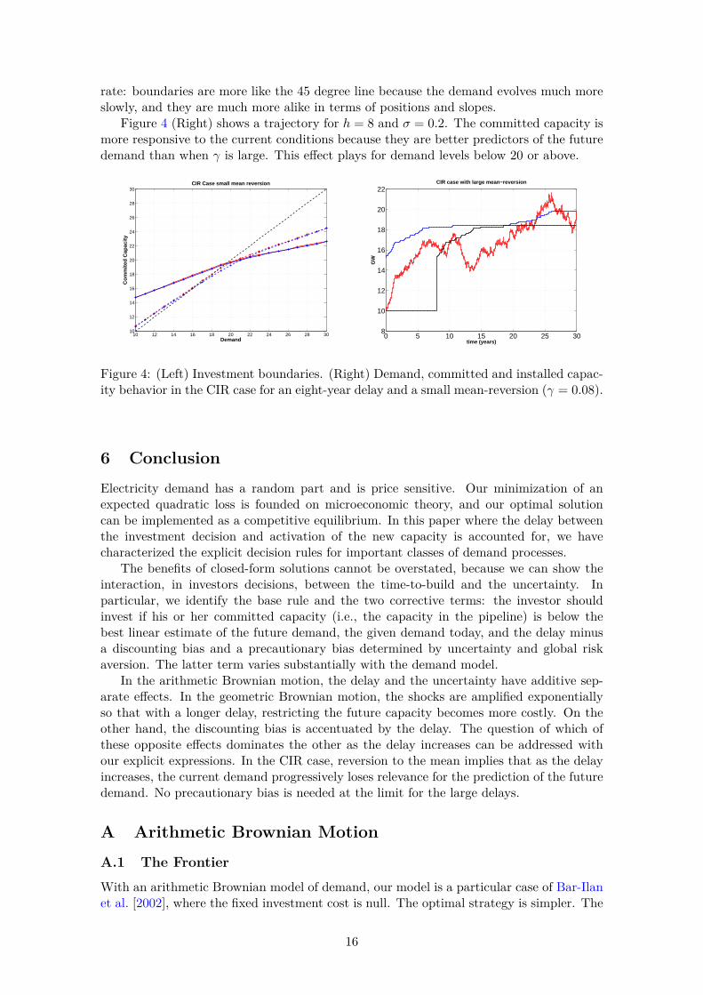
rate: boundaries are more like the 45 degree line because the demand evolves much moreslowly, and they are much more alike in terms of positions and slopes.

Figure 4 (Right) shows a trajectory for h = 8 and σ = 0.2. The committed capacity ismore responsive to the current conditions because they are better predictors of the futuredemand than when γ is large. This effect plays for demand levels below 20 or above.

10 12 14 16 18 20 22 24 26 28 3010

12

14

16

18

20

22

24

26

28

30

Co

mm

ited

Cap

acit

y

Demand

CIR Case small mean reversion

0 5 10 15 20 25 308

10

12

14

16

18

20

22

GW

time (years)

CIR case with large mean−reversion

Figure 4: (Left) Investment boundaries. (Right) Demand, committed and installed capac-ity behavior in the CIR case for an eight-year delay and a small mean-reversion (γ = 0.08).

6 ConclusionElectricity demand has a random part and is price sensitive. Our minimization of anexpected quadratic loss is founded on microeconomic theory, and our optimal solutioncan be implemented as a competitive equilibrium. In this paper where the delay betweenthe investment decision and activation of the new capacity is accounted for, we havecharacterized the explicit decision rules for important classes of demand processes.

The benefits of closed-form solutions cannot be overstated, because we can show theinteraction, in investors decisions, between the time-to-build and the uncertainty. Inparticular, we identify the base rule and the two corrective terms: the investor shouldinvest if his or her committed capacity (i.e., the capacity in the pipeline) is below thebest linear estimate of the future demand, the given demand today, and the delay minusa discounting bias and a precautionary bias determined by uncertainty and global riskaversion. The latter term varies substantially with the demand model.

In the arithmetic Brownian motion, the delay and the uncertainty have additive sep-arate effects. In the geometric Brownian motion, the shocks are amplified exponentiallyso that with a longer delay, restricting the future capacity becomes more costly. On theother hand, the discounting bias is accentuated by the delay. The question of which ofthese opposite effects dominates the other as the delay increases can be addressed withour explicit expressions. In the CIR case, reversion to the mean implies that as the delayincreases, the current demand progressively loses relevance for the prediction of the futuredemand. No precautionary bias is needed at the limit for the large delays.

A Arithmetic Brownian Motion

A.1 The Frontier

With an arithmetic Brownian model of demand, our model is a particular case of Bar-Ilanet al. [2002], where the fixed investment cost is null. The optimal strategy is simpler. The

16

demand dynamics are:

dDt = µdt+ σdWt, µ ∈ R, σ > 0, (74)

then O = R and (13) is verified with κ1 = ε for each ε > 0. Therefore, according to (25),we assume that ρ > 0. Thus,

[Lφ](d) = ρφ(d)− µφ′(d)− 12σ

2φ′′(d), φ ∈ C2(O). (75)

The increasing fundamental solution to Lφ = 0 is ψ(d) = eλd where λ is the positivesolution to

ρ− µλ− 12σ

2λ2 = 0. (76)

Because, in this case,

β0(d) = d+ µh and β(d) = µh

ρ+ d

ρ+ µ

ρ2 . (77)

Due to Theorem 1, c is affine:

c(d) = d+ µh− q0ρeρh −

√µ2 + 2ρσ2 − µ

2ρ . (78)

A.2 Comparative statics

Consider that∂2c(d)∂h∂σ

= 0. (79)

Whatever the time to build h, the investment is retarded in the same way by an increasein σ, and conversely. This additive separability makes it difficult to find the cross effectsbetween the uncertainty and the delay with this model, contrary to Bar-Ilan et al. [2002].

An increase in uncertainty always retards investment:

∂c(d)/∂σ = − σ√µ2 + 2ρσ2 < 0. (80)

The variation of c(d) with respect to the time-to-build h is

∂c(d)/∂h = µ− q0ρ2eρh. (81)

The effect is to hasten investment if µ is relatively large. If h is relatively large, thenthe cost of investment appears large compared to the future discounted damage, andinvestment is retarded. We retrieve the effects encountered in the case of the geometricBrownian motion.

Furthermore,

∂c(d)/∂µ = h+ 12ρ

(1− µ√

µ2+2ρσ2

)> 0, (82)

and

∂c(d)/∂ρ = −q0(1 + hρ)eρh + 12

(µ2 + ρσ2 − µ

√µ2 + 2ρσ2

ρ2√µ2 + 2ρσ2

). (83)

In the latter expression, the first term is negative (the discounting bias is reinforced),whereas the second term is positive (the precautionary bias is attenuated). Thus, we getthe same effects encountered in the case of the geometric Brownian motion.

17

A.3 Simulations

On Figure 5 (Left), b := c(d)− d is given as a function of σ, for two contrasted values ofh (1 and 8 years). The other parameters are: ρ = 0.08, µ = 300, with an initial demandof 10,000 MW and demand, committed capacity, and installed capacity all equal at date0 (D0 = C0 = K0).

Figure 5 (Left) shows that the impact of the time-to-build with these values is muchmore important than the impact of uncertainty. Indeed, numerically, ∂c(d)/∂h is of theorder of 300 whereas ∂c(d)/∂σ is of the order of −1. The first effect largely dominates.

By and large, this result is in line with Bar-Ilan et al. [2002]. In their setting, increasingthe time-to-build from one year to eight years reverses the relation between uncertaintyand investment, which is possible only because they are not separable. Specifically, for along delay, an increase in uncertainty hastens investments but decreases their level. But,these effects are very small (Bar-Ilan et al. [2002, pp. 85, Figure 2]).

The excess of committed capacity does not imply that the system will hold an excessof installed capacity. In fact, the reverse is observed in Figure 5 (Right). In the case ofa delay of eight years, an excess of committed capacity as measured by the value of b is1,873 MW. But in eight years, the demand will grow on average 2,400 MW, which clearlyindicates that the optimal strategy is to avoid excess installed capacity.

100 200 300 400 500 600-500

0

500

1000

1500

2000

2500

σ

b

h = 1h = 8

0 10 20 30 400.8

1

1.2

1.4

1.6

1.8

2

2.2x 104

time (years)

demandcommitted capacityinstalled capacity

Figure 5: (Left) c(d) − d as a function of σ for two values of the time-to-build, h = 1(blue crosses) and h = 8 (red circles). (Right) Demand, committed and installed capacitybehavior for an eight-year delay, σ = 600 MW·year1/2.

B Proof of Proposition 2Let (c, d) ∈ S. We prove first that

vc(c, d) =E[∫ +∞

0e−ρtgc(Cc,∗t , Dd

t )dt], (84)

where C∗ is the optimal state process associated to the optimal control I∗ provided byTheorem 1. Let I∗ ∈ I be optimal for (c, d). Therefore,

G(c+ ε, d; I∗)−G(c, d; I∗)ε

≥ v(c+ ε, d)− v(c, d)ε

. (85)

On the other hand,

G(c+ ε, d; I∗)−G(c, d : I∗)ε

= E[∫ +∞

0e−ρt

g(Cc,I∗

t + ε,Ddt )− g(Cc,I

∗

t , Ddt )

εdt]. (86)

18

Taking the limsup in (85) and taking into account (86), we get

lim supε↓0

v(c+ ε, d)− v(c, d)ε

≤ E[∫ ∞

0e−ρtgc(Cc,∗t , Dd

t )dt]. (87)

On the other hand, arguing symmetrically with c− ε, we get

lim infε↓0

v(c, d)− v(c− ε, d)ε

≥ E[∫ +∞

0e−ρtgc(Cc,∗t , Dd

t )dt]. (88)

Therefore, (87) and (88) assert (84).Because of equation (84), vc ≥ −q0, the definition of A, and because of

gc(Cc,∗t , Ddt ) = e−ρhE

[c−Dd

h

]; (89)

the quadratic surplus application based on equation (1) as an expected discounted revenue(price minus marginal cost) yields the result.

ReferencesM. Abramowitz and I.A. Stegun, eds., Handbook of Mathematical Functions with Formulas, Graphs,

and Mathematical Tables. Chapter 13, New York: Dover, 1965.

F.L. Aguerrevere. Equilibrium Investment Strategies and Output Price Behavior: A Real-OptionsApproach. Review of Financial Studies, 16(4): 1239–1272, 2003.

A. Bar-Ilan and W.C. Strange. Investment Lags. American Economic Review, 86(3): 610–623,June 1996.

A. Bar-Ilan, A. Sulem, and A. Zanello. Time-to-Build and Capacity Choice. Journal of EconomicDynamics and Control, 26: 69–98, 2002.

B. Bruder and H. Pham. Impulse Control Problem on Finite Horizon with Execution Delay.Stochastic Processes and their Applications, 119: 1436-1469, 2009.

S. Federico and H. Pham. Characterization of the Optimal Boundaries in Reversible InvestmentProblems. 2014. To appear in SIAM Journal of Control and Optimization.

G. Ferrari. On an Integral Equation for the Free-Boundary of Stochastic, Irreversible InvestmentProblems. 2013. To appear in Annals of Applied Probability.

S.R. Grenadier. Equilibrium with Time-to-Build: A Real Options Approach. Project Flexibility,Agency and Competition. M. Brennan and L. Trigeorgis (eds), Oxford University Press, 2000.

S.R. Grenadier. Option Exercise Games: An Application to the Equilibrium Investment Strategiesof Firms. Review of Financial Studies, 15(3): 691–721, 2002.

N. Ikeda and S. Watanabe. Stochastic Differential Equations and Diffusion Processes. North-Holland, 1981.

I. Karatzas and S.E. Shreve. Brownian Motion and Stochastic Calculus. Springer-Verlag, 1991.

N.V. Krylov. Controlled Diffusion Processes. Springer-Verlag, 1980.

S. Majd and R.S. Pindyck. Time-to-Build, Option Value and Investment Decisions. Journal ofFinancial Economics, 18: 7–27, 1986.

R. McDonald and D. Siegel. The Value of Waiting to Invest. Quarterly Journal of Economics,101: 707–727, 1986.

A. Milne and A.E. Whalley. ‘Time to Build, Option Value and Investment Decisions’: A Comment.Journal of Financial Economics, 56: 325–332, 2000.

19

G. Pacheco de Almeida and P. Zemsky. The Effect of Time-to-Build on Strategic Investment underUncertainty. RAND Journal of Economics, 34(1): 166–182, 2003.

L.C.G. Rogers and D. Williams. Diffusions, Markov Processes and Martingales. Vol. 2: ItôCalculus, 2nd Edition (2000), Cambridge University Press.

20