EXPLICIT DECONVOLUTION OF WELLBORE STORAGE DISTORTED WELL TEST DATA A Thesis by OLIVIER BAHABANIAN Submitted to the Office of Graduate Studies of Texas A&M University in partial fulfillment of the requirements for the degree of MASTER OF SCIENCE December 2006 Major Subject: Petroleum Engineering

Welcome message from author
This document is posted to help you gain knowledge. Please leave a comment to let me know what you think about it! Share it to your friends and learn new things together.
Transcript
EXPLICIT DECONVOLUTION OF
WELLBORE STORAGE DISTORTED WELL TEST DATA
A Thesis
by
OLIVIER BAHABANIAN
Submitted to the Office of Graduate Studies of Texas A&M University
in partial fulfillment of the requirements for the degree of
MASTER OF SCIENCE
December 2006
Major Subject: Petroleum Engineering
EXPLICIT DECONVOLUTION OF
WELLBORE STORAGE DISTORTED WELL TEST DATA
A Thesis
by
OLIVIER BAHABANIAN
Submitted to the Office of Graduate Studies of Texas A&M University
in partial fulfillment of the requirements for the degree of
MASTER OF SCIENCE Approved by:
Chair of Committee, Thomas A. Blasingame Committee Member, Jerry L. Jensen Wayne M. Ahr Head of Department, Stephen A. Holditch
December 2006
Major Subject: Petroleum Engineering
iii
ABSTRACT
Explicit Deconvolution of Wellbore Storage Distorted Well Test Data. (December 2006)
Olivier Bahabanian,
Diplôme d’Ingénieur Civil, Ecole des Mines de Paris
Chair of Advisory Committee: Dr. Thomas A. Blasingame The analysis/interpretation of wellbore storage distorted pressure transient test data remains one of the
most significant challenges in well test analysis. Deconvolution (i.e., the "conversion" of a variable-rate
distorted pressure profile into the pressure profile for an equivalent constant rate production sequence) has
been in limited use as a "conversion" mechanism for the last 25 years. Unfortunately, standard decon-
volution techniques require accurate measurements of flow-rate and pressure — at downhole (or sandface)
conditions. While accurate pressure measurements are commonplace, the measurement of sandface flow-
rates is rare, essentially non-existent in practice.
As such, the "deconvolution" of wellbore storage distorted pressure test data is problematic.
In theory, this process is possible, but in practice, without accurate measurements of flowrates, this
process can not be employed. In this work we provide explicit (direct) deconvolution of wellbore storage
distorted pressure test data using only those pressure data. The underlying equations associated with each
deconvolution scheme are derived in the Appendices and implemented via a computational module.
The value of this work is that we provide explicit tools for the analysis of wellbore storage distorted
pressure data; specifically, we utilize the following techniques:
Russell method (1966) (very approximate approach),
"Beta" deconvolution (1950s and 1980s),
"Material Balance" deconvolution (1990s).
Each method has been validated using both synthetic data and literature field cases and each method
should be considered valid for practical applications.
Our primary technical contribution in this work is the adaptation of various deconvolution methods for the
explicit analysis of an arbitrary set of pressure transient test data which are distorted by wellbore storage
— without the requirement of having measured sandface flowrates.

iv
DEDICATION
We must never be afraid to go too far, for truth lies beyond.
— Marcel Proust
He who loves practice without theory is like the sailor who boards ship without a rudder and compass, and never knows where he may cast.
— Leonardo da Vinci

v
ACKNOWLEDGEMENTS
I want to express my gratitude and appreciation to:
Dr. Tom Blasingame for his support and guidance during my research and graduate studies.
Dr. Jerry Jensen for his support and guidance during my research and graduate studies.
Dr. Wayne Ahr for serving as a member of my advisory committee.
Dilhan Ilk for his selfless help during the later stages of my research.
vi
TABLE OF CONTENTS
Page
ABSTRACT ......................................................................................................................................... iii
DEDICATION ..................................................................................................................................... iv
ACKNOWLEDGEMENTS.................................................................................................................. v
TABLE OF CONTENTS ..................................................................................................................... vi
LIST OF FIGURES.............................................................................................................................. viii
CHAPTER
I INTRODUCTION ............................................................................................................ 1
1.1 Research Problem............................................................................................ 1 1.2 Research Objective.......................................................................................... 1 1.3 Previous Work................................................................................................. 1 1.4 Summary ......................................................................................................... 3
II THE WELLBORE STORAGE DISTORTION OF WELL TEST DATA ....................... 4
2.1 Wellbore Effects on a Well Test ..................................................................... 4 2.2 The Wellbore Storage Effect ........................................................................... 5
2.2.1 Theoretical Developments............................................................. 6 2.2.2 Practical Issues .............................................................................. 7
2.3 Sandface Flowrate Estimators ......................................................................... 7 2.4 Theoretical Development: Superposition Principle and Convolution ............. 8
III EXPLICIT METHODS FOR THE ANALYSIS OF WELLBORE STORAGE DISTORTED WELL TEST DATA.................................................................................. 10
3.1 Russell Method (1966) .................................................................................... 10 3.2 Rate Normalization ......................................................................................... 10 3.3 Material Balance Deconvolution..................................................................... 11 3.4 β ("Beta") Deconvolution ................................................................................ 11
IV EXAMPLE APPLICATIONS .......................................................................................... 13
4.1 Demonstration using a Synthetic Data Case.................................................... 13 4.2 Demonstration using a Field Case................................................................... 14
V SUMMARY, CONCLUSIONS, AND RECOMMENDATIONS FOR FUTURE WORK .............................................................................................................................. 17
5.1 Summary and Conclusions.............................................................................. 17
vii
Page
5.2 Recommendations for Future Work ................................................................ 19
NOMENCLATURE............................................................................................................................. 20
REFERENCES..................................................................................................................................... 22
APPENDIX A RUSSELL METHOD FOR "CORRECTION" OF WELL TEST DATA
DISTORTED BY WELLBORE STORAGE (RUSSELL, 1966)........................... 25
APPENDIX B DERIVATION OF THE β-DECONVOLUTION FORMULATION .................... 31
APPENDIX C DERIVATION OF THE COEFFICIENTS FOR β-DECONVOLUTION............. 34
APPENDIX D MATERIAL BALANCE DECONVOLUTION RELATIONS FOR
WELLBORE STORAGE DISTORTED PRESSURE TRANSIENT DATA ........ 39
APPENDIX E IMPLEMENTATION STRUCTURE AND VALIDATION OF THE
COMPUTATIONAL MODULE............................................................................ 41
VITA .................................................................................................................................................... 45
viii
LIST OF FIGURES
FIGURE Page
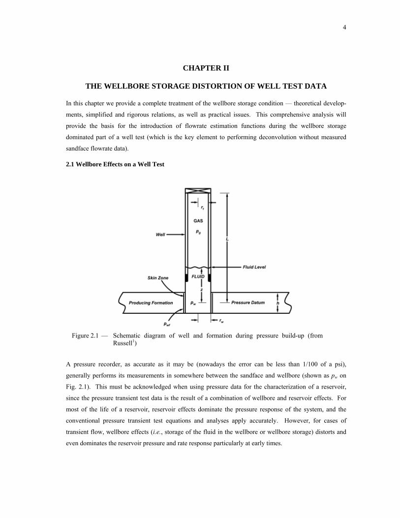
2.1 Schematic diagram of well and formation during pressure build-up (from Russell1) .............. 4
2.2 Typical pressure buildup plot (from Russell1).......................................................................... 5
4.1 Synthetic example using various deconvolution techniques (infinite-acting reservoir case
with wellbore storage effects) .................................................................................................. 13
4.2 (Semilog plot) Bourdet24 field example using various deconvolution techniques (infinite-
acting reservoir case with wellbore storage effects)................................................................. 15
4.3 (Log-log plot) Bourdet24 field example using various deconvolution techniques (infinite-
acting reservoir case with wellbore storage effects)................................................................. 16
1
CHAPTER I
INTRODUCTION
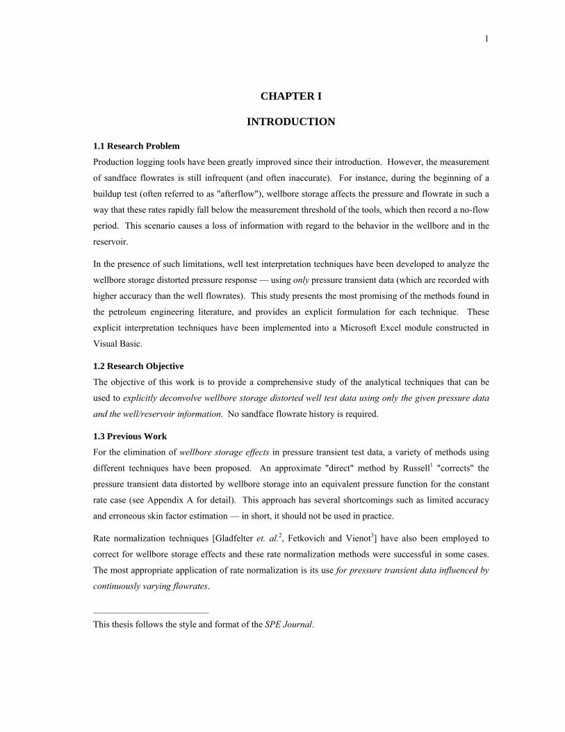
1.1 Research Problem
Production logging tools have been greatly improved since their introduction. However, the measurement
of sandface flowrates is still infrequent (and often inaccurate). For instance, during the beginning of a
buildup test (often referred to as "afterflow"), wellbore storage affects the pressure and flowrate in such a
way that these rates rapidly fall below the measurement threshold of the tools, which then record a no-flow
period. This scenario causes a loss of information with regard to the behavior in the wellbore and in the
reservoir.
In the presence of such limitations, well test interpretation techniques have been developed to analyze the
wellbore storage distorted pressure response — using only pressure transient data (which are recorded with
higher accuracy than the well flowrates). This study presents the most promising of the methods found in
the petroleum engineering literature, and provides an explicit formulation for each technique. These
explicit interpretation techniques have been implemented into a Microsoft Excel module constructed in
Visual Basic.
1.2 Research Objective
The objective of this work is to provide a comprehensive study of the analytical techniques that can be
used to explicitly deconvolve wellbore storage distorted well test data using only the given pressure data
and the well/reservoir information. No sandface flowrate history is required.
1.3 Previous Work
For the elimination of wellbore storage effects in pressure transient test data, a variety of methods using
different techniques have been proposed. An approximate "direct" method by Russell1 "corrects" the
pressure transient data distorted by wellbore storage into an equivalent pressure function for the constant
rate case (see Appendix A for detail). This approach has several shortcomings such as limited accuracy
and erroneous skin factor estimation — in short, it should not be used in practice.
Rate normalization techniques [Gladfelter et. al.2, Fetkovich and Vienot3] have also been employed to
correct for wellbore storage effects and these rate normalization methods were successful in some cases.
The most appropriate application of rate normalization is its use for pressure transient data influenced by
continuously varying flowrates.
_________________________
This thesis follows the style and format of the SPE Journal.
2
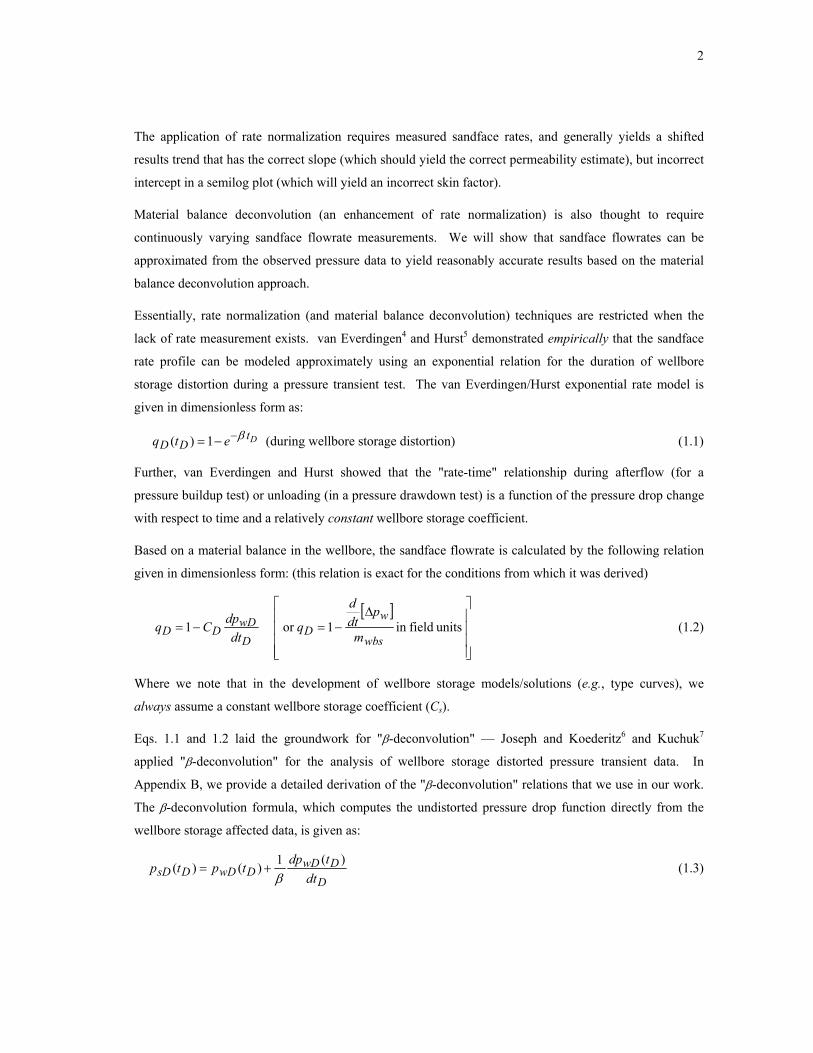
The application of rate normalization requires measured sandface rates, and generally yields a shifted
results trend that has the correct slope (which should yield the correct permeability estimate), but incorrect
intercept in a semilog plot (which will yield an incorrect skin factor).
Material balance deconvolution (an enhancement of rate normalization) is also thought to require
continuously varying sandface flowrate measurements. We will show that sandface flowrates can be
approximated from the observed pressure data to yield reasonably accurate results based on the material
balance deconvolution approach.
Essentially, rate normalization (and material balance deconvolution) techniques are restricted when the
lack of rate measurement exists. van Everdingen4 and Hurst5 demonstrated empirically that the sandface
rate profile can be modeled approximately using an exponential relation for the duration of wellbore
storage distortion during a pressure transient test. The van Everdingen/Hurst exponential rate model is
given in dimensionless form as:
DtDD etq 1)( β−−= (during wellbore storage distortion) (1.1)
Further, van Everdingen and Hurst showed that the "rate-time" relationship during afterflow (for a
pressure buildup test) or unloading (in a pressure drawdown test) is a function of the pressure drop change
with respect to time and a relatively constant wellbore storage coefficient.
Based on a material balance in the wellbore, the sandface flowrate is calculated by the following relation
given in dimensionless form: (this relation is exact for the conditions from which it was derived)
DwD
DD dtdpCq −= 1
[ ]
⎥⎥⎥⎥
⎦
⎤
⎢⎢⎢⎢
⎣
⎡ ∆−= units fieldin 1or
wbs
wD m
pdtd
q (1.2)
Where we note that in the development of wellbore storage models/solutions (e.g., type curves), we
always assume a constant wellbore storage coefficient (Cs).
Eqs. 1.1 and 1.2 laid the groundwork for "β-deconvolution" — Joseph and Koederitz6 and Kuchuk7
applied "β-deconvolution" for the analysis of wellbore storage distorted pressure transient data. In
Appendix B, we provide a detailed derivation of the "β-deconvolution" relations that we use in our work.
The β-deconvolution formula, which computes the undistorted pressure drop function directly from the
wellbore storage affected data, is given as:
DDwD
DwDDsD dttdp
tptp)(1)()(
β+= (1.3)
3
We note that Eq. 1.3 is only valid when the sandface flowrate profile follows an exponential trend as
prescribed by Eq.1.1. In this work, our objective is to generalize Eq. 1.3 by treating β as a variable [β(t) or
β(tD)], rather than as a constant. We develop several schemes to perform "β-deconvolution" directly using
pressure derivative and/or pressure integral and integral-derivative functions. We describe these schemes
in detail in Appendix C.
Once we obtain the β(tD) function, we utilize Eq. 1.3 as the mechanism for directly estimating the
"undistorted pressure drop" function. The obvious advantage of "β-deconvolution" is that the wellbore
storage effects are eliminated using only the given pressure data.
1.4 Summary
This study begins with an in-depth analysis of the wellbore storage condition — theoretical developments,
simplified and rigorous relations, and practical issues. The methods introduced previously are then
derived explicitly (specifically — the Russell method (Appendix A), the β-deconvolution model
(Appendix B), the β-deconvolution coefficients (Appendix C), and the explicit rate normalization and
material balance deconvolution methods (Appendix D). These formulations are then implemented into
Microsoft Excel computation/interface module (description provided in Appendix E).
Synthetic and field data cases are used within the computation module to assess the behavior,
performance, and possible shortcomings of each explicit deconvolution method. The primary product of
this thesis is a workflow for the correction of well test data distorted by wellbore storage without the
requirement of measured flowrates. The individual deconvolution methods are relevant for discussion and
evaluation and the computational module is a major accomplishment as well, but (again) the most
important aspect of this work is the process (or workflow) that one must consider in order to perform
deconvolution of well test data distorted by wellbore storage effects.
For the purposes of inventory, we note that in this work we utilize the explicit deconvolution methods
given below:
Rate Normalization (approximate) Material Balance Deconvolution (rigorous for monotonic rate functions) Beta Deconvolution (rigorous for exponential rate functions)
4
CHAPTER II
THE WELLBORE STORAGE DISTORTION OF WELL TEST DATA
In this chapter we provide a complete treatment of the wellbore storage condition — theoretical develop-
ments, simplified and rigorous relations, as well as practical issues. This comprehensive analysis will
provide the basis for the introduction of flowrate estimation functions during the wellbore storage
dominated part of a well test (which is the key element to performing deconvolution without measured
sandface flowrate data).
2.1 Wellbore Effects on a Well Test
Figure 2.1 — Schematic diagram of well and formation during pressure build-up (from Russell1)
A pressure recorder, as accurate as it may be (nowadays the error can be less than 1/100 of a psi),
generally performs its measurements in somewhere between the sandface and wellbore (shown as pw on
Fig. 2.1). This must be acknowledged when using pressure data for the characterization of a reservoir,
since the pressure transient test data is the result of a combination of wellbore and reservoir effects. For
most of the life of a reservoir, reservoir effects dominate the pressure response of the system, and the
conventional pressure transient test equations and analyses apply accurately. However, for cases of
transient flow, wellbore effects (i.e., storage of the fluid in the wellbore or wellbore storage) distorts and
even dominates the reservoir pressure and rate response particularly at early times.

5
A schematic case of wellbore storage effects imposed on a system is illustrated in the pressure response
shown in Fig. 2.2. A complete knowledge of these "wellbore effects" would permit the "correction" of
these effects (using a process known as "deconvolution") which would provide interpretation and analysis
of well tests for early and very early data (as these are the most distorted data). Simply put, the goal of
this work (and of deconvolution in general) is to correct the pressure data taken at early times which are
affected by "wellbore storage." Lacking the ability to "correct" these data means that we must wait for the
distortion of the data to diminish (sometimes only a few hours, but possibly months or years for very low
permeability gas reservoirs). As well tests are often run for as short as economically feasible for a
particular well, many well tests are often completely distorted by wellbore storage effects.
Figure 2.2 — Typical pressure buildup plot (from Russell1).
These "wellbore" effects have been labeled as "wellbore dynamics" by Mattar and Santo8, and these
effects include the following components: (one or more effects may act at any given time)
Liquid influx/efflux. Phase redistribution. Wellbore and near-wellbore cleanup. Plugging. Recorder effects: drift, hysteresis, malfunction, temperature sensitivity, and fluid PVT changes. Gas/oil solution/liberation. Retrograde condensation. Diverse effects such as leaks, geotidal/microseismic.
6
2.2 The Wellbore Storage Effect
Since its introduction by van Everdingen and Hurst9 in 1949, the issue of wellbore storage distortion has
been extensively treated in the Petroleum Engineering literature. In 1970, Agarwal et al.10 and Watten-
barger and Ramey11 provided the theoretical detail (as well as analytical and numerical solutions) to
support the base relations put forth by van Everdingen and Hurst9. The theoretical issues are relatively
straightforward, the wellbore and reservoir are separate models coupled together, influences in the
wellbore affect the reservoir and vice-versa. For the purpose of this work we treat the "simple" case of a
constant wellbore storage behavior. This condition should be applicable in the vast majority of cases in
practice, and it provides us a basis for extending beyond the constant wellbore storage case in later work.
2.2.1 Theoretical Developments
Whenever a well is shut in, fluid from the formation will flow into the wellbore until equilibrium condi-
tions are reached. Similarly, a part of the fluid produced when a well is put on production is the fluid that
was present is the wellbore prior to the opening of the well. This "ability of the well to store and unload
fluids" (Raghavan12) is the definition of wellbore storage.
dtdp
BCq wf
wb −= (2.1)
Where qwb represents the rate at which the wellbore "unloads" fluids, and C represents the storage constant
of the well. In the specific case where the wellbore unloading is entirely due to fluid expansion, then the
wellbore storage constant is defined by: (Ramey13)
pVC
∆∆
= (2.2)
Where ∆V is the change in volume of fluid in the wellbore — at wellbore conditions — and ∆p is the
change in bottomhole pressure.
When the wellbore is filled with a single fluid phase, Eq. 2.2 becomes
cVC w= (2.3)
where Vw is the total wellbore volume and c is the compressiblility of the fluid in the wellbore at wellbore
conditions. The use of dimensionless pressure functions in most of the derivations of this work leads to
the use of a dimensionless wellbore storage coefficient, CD.
2894.0wt
DhrcCC
φ= (2.4)
As such, wellbore storage affects the sandface flowrate, causing a lag in the sandface flowrate relative to
any change in the surface flowrate. The surface flowrate is the sum of the wellbore rate (qwb) and the
sandface rate (qsf) — i.e., the sum of the wellbore (unloading) rate and the sandface flowrate:
wbsf qqq += (2.5)
7
van Everdigen and Hurst9 expressed the rigorous sandface flowrate relation for wellbore storage and skin
using constant wellbore storage coefficient. The relation is given in dimensionless form as:
DwD
DDD dtdp
Ctq −= 1)( (1.2)
We will make frequent use of this relation in this study, since it directly links the sandface flowrate (for
which we do not have any direct measurements) to the wellbore pressure (for which we typically do have
direct and accurate measurements).
2.2.2 Practical Issues
For more than 40 years, a time-dependent wellbore storage profile has been reported in the technical
literature [Hegeman et al.14]. When this phenomenon occurs, it makes the application of well test analysis
techniques which are based on the constant wellbore storage assumption — such as type-curve matching
— very difficult. A changing wellbore storage condition occurs when the fluid compressibility in the
wellbore (c, defined in Eq. 2.3) varies with changing pressure (or more appropriately, time). Fortunately,
such variations in the wellbore storage coefficient are most often negligible. Well tests strongly affected
by this phenomenon include occurrences of wellbore phase redistribution (segregation), and injection well
testing.
2.3 Sandface Flowrate Estimators
Blasingame et al.15 proposed five different methods of calculating sandface rates from pressure data for
the constant wellbore storage case. These methods will be useful in the implementation of the
computational module since most of the implemented methods require the knowledge (or an estimate) of
the sandface flowrates.
Method 1: Definition of sandface flowrate (exact)
[ ]
wbs
w
DwD
DD m
pdtd
dtdp
Cq∆
−=−= 11 (1.2)
Method 2: Alternative calculation of sandface flowrate based on Method 1 (exact)
wbsw
wDDDD mp
tpCtQ∆
−=−= (2.6)
[ ])(1
tQdtdq DD = (2.7)
Method 3: Average sandface flowrate calculation (exact)
tp
mtpCq w
wbsDwD
DDi∆
−=−=111 (1.2)

8
2D
Dtt
i= (2.8)
Method 4: Semi-empirical sandface flowrate calculation — assumes CD = tD/pwD (approximate)
[ ]pdtd
pt
dtdp
ptq
wDwD
wDD
D ∆∆
−=−= 112
(2.9)
22
DD
tt = (2.10)
Method 5: Semi-empirical sandface flowrate calculation — assumes CD = tD/pwDi (approximate)
[ ]wiwiwDi
wDiwDwDi
wDidD p
dtd
pt
ppp
ppq ∆
∆−=
−−=−= 111
3 (2.11)
43
DD
tt = (2.12)
2.4 Theoretical Development: Superposition Principle and Convolution
Convolution is a mathematical operator which, using two functions f and g, produces a third function
commonly noted as f*g representing the amount of overlap between f and a reversed and shifted version of
g. The convolution operation is defined as:
τττ dtgftgft
)()()()*(0
−= ∫ (2.13)
The convolution operation can by expressed in discrete form as:
∑=
−− ∆−≈n
iii tgftgf
111 )()())(*( τττ (2.14)
The principle of superposition (or convolution) states that, for a linear system, a linear combination of
solutions for a system is also a solution to the same linear system. The superposition (or convolution)
principle applies to linear systems of algebraic equations, and for our field of study — linear partial
differential equations (i.e., the diffusivity equation for flow in porous media)
In well test analysis, the superposition principle is used to construct reservoir response functions, to
represent various reservoir boundaries (by superposition in space), and to determine variable rate reservoir
responses (using superposition in time). However, we must always keep in mind when applying this
principle that it is only valid for linear systems that is when nonlinearities are present (e.g. gas flow),
principle of superposition is not directly applicable. In those cases linearization (via the pseudopressure
transform) must be performed in order to apply the superposition principle to the tranformed system.
The early work by Duhamel16 on heat transfer has since then been used in numerous engineering domains.
Adapted to our domain, petroleum engineering, Duhamel's principle states that the observed pressure drop
9
is the convolution of the input rate function and the derivative of the constant-rate pressure response — at
t=0 the system is assumed to be in equilibrium (i.e., p(r,t=0) = pi).
For reference, the convolution integral is defined as:
τdτpτtqt
tp u )(')(0
)( −=∆ ∫ (2.15)
Eq. 2.15 can be written in a discrete form by assuming that the rate change can be discretized as a series of
rate changes:
))(()()( 111
−−=
−−=∆ ∑ iuin
ii ttpqqtp (2.16)
van Everdingen and Hurst8 introduced the use of Duhamel's principle in the analysis of variable-rate well-
test data and they utilized Duhamel's principle to obtain dimensionless wellbore pressure-drop responses
for a continuously (smoothly) varying flowrate. The underlying idea was to introduce a method to
convolve/superimpose the constant rate pressure response with a continuous (smooth) rate profile to
produce the variable rate wellbore pressure-drop response.
Odeh and Jones17, Agarwal18, Soliman19, Stewart, Wittman and Meunier20, Fetkovich and Vienot3, among
others, applied the convolution guidelines in various settings. However, these methods are inherently
restricted by the use of a particular model for the constant rate pressure function (i.e., presumed reservoir
model) used in the convolution integral.
10
CHAPTER III
EXPLICIT METHODS FOR THE ANALYSIS
OF WELLBORE STORAGE DISTORTED WELL TEST DATA
This work was put forth as an attempt to provide a set of simple, explicit deconvolution formulas that
could be used on wellbore storage distorted pressure transient test data. We evaluated a very old
"correction" method by Russell1 and found this method to be unacceptable for all applications. We also
evaluated the "material balance deconvolution" [Johnston21] for the purpose of evaluating pressure
transient test data without any sandface rate information. This approach was successful and should be
considered sufficiently accurate to be used as a standard tool for field applications.
The other "major" method considered was the direct β-deconvolution algorithm modified to estimate the
β-parameter from pressure rather than flowrate data as originally proposed by van Everdingen4 and Hurst 5. The modification of the β-deconvolution algorithm (given only in terms of pressure variables) was also
successful.
3.1. Russell Method (1966): The pressure "correction" function given by Russell1 is given as:
)(log)hr 1(11
)]0()([
2
tmtf
tC
tptpsl
wfws ∆+=∆=
⎥⎦
⎤⎢⎣
⎡∆
−
=∆−∆ (3.1)
Where the C2-term is derived rigorously using Russell's assumptions of the system. The C2-term is used as
an arbitrary constant to be optimized. In short, the Russell method has an elegant mathematical
formulation, but ultimately, we believe that this formulation does not represent the wellbore storage condi-
tion, and hence, we do not recommend the Russell method under any circumstances.
3.2. Rate Normalization
Gladfelter, Tracy and Wilsey2 introduced the "rate normalization" deconvolution approach — which, in
their words "permits direct measurement of the cause of low well productivity." The objective of rate
normalization is to remove/correct the effects of the variable rate from the observed pressure data. Rate
normalization can also be defined as an approximation to convolution integral (Raghavan11).
)()()( tptqtp u≈∆ (3.2)
Where pu is the constant rate pressure response. Rate normalization has been employed for a number of
applications in well test analysis. For the specific application of "rate normalization" deconvolution, we
must recognize that the approach is approximate — and while this method does provide some "correction"
capabilities, it is basically a technique that can be used for pressure data influenced by continuously
varying flowrates. Most notably, Fetkovich and Vienot3, Winestock and Colpitts22 (1965, pressure
11
transient test analysis) and Doublet et al.23 (1994, production data analysis) have demonstrated the
effectiveness of "rate normalization" deconvolution (albeit for specialized cases). In particular, for the
wellbore storage domination and distortion regimes, rate normalization can provide a reasonable
approximation of the no wellbore storage solution. For this inifinite-acting radial flow case, rate
normalization yields an erroneous estimate of the skin factor by introducing a shift on the semilog straight
line (obvioulsy, the sandface rate profile must be known). This last point, however, makes the application
of rate normalization techniques very limited in our particular problem — we do not have measurements
of sandface flowrate. Therefore, this method must be applied using an estimate of the downhole rate (see
rate estimation relations in Chapter II) — which will definitely introduce errors in the deconvolution
process. Such issues make rate normalization a "zero-order" approximation — that is, rate normalization
results should be considered as a guide, but not relied upon as the best methodology.
3.3. Material Balance Deconvolution
The relations for the deconvolution of wellbore storage distorted well test data using material balance
deconvolution are provided in Appendix D. The wellbore storage-based, material balance time function
for the pressure buildup case is given as:
][11
1
1 ,
,,,
wswbs
wswbs
BUwbs
BUwbspBUmb
ptd
dm
pm
t
qN
t∆
∆−
∆−∆=
−=∆ (3.3)
And the wellbore storage-based, rate-normalized pressure drop function for the pressure buildup case is
given as:
wsws
wbsBUwbs
wsBUs p
ptd
dm
qp
p ∆∆
∆−
=−
∆=∆
][11
11 ,
, (3.4)
In the material balance deconvolution formulation the ∆tmb,BU function is used in place of the time function,
in whatever fashion is required — plotting data functions, modeling, etc. And the ∆ps,BU function is used
as a pressure drop function — in any appropriate manner that pressure drop would be employed.
3.4. β ("Beta") Deconvolution
We also present the application of our new β-deconvolution algorithm derived from wellbore-storage
distorted pressure functions (see Appendices B and C). The final result developed for application in our
present work is given by: (this is the general form for pressure drawdown or buildup cases).
widwdw
wdws p
ppppp ∆
∆−∆∆
+∆=∆)(
(3.5)
12
Where, for the pressure buildup case, we have:
)0( =∆−=∆ tppp wfwsw (pressure drop) (3.6)
tdpd
tp wwd ∆
∆∆=∆ (pressure drop derivative) (3.7)
τdpt
tp wwi ∆
∆
∆=∆ ∫0
1 (pressure drop integral) (3.8)
tdpd
tp wiwid ∆
∆∆=∆ (pressure drop integral-derivative) (3.9)
The more "rigorous" β-deconvolution algorithm [i.e., where an exponential rate profile is required (Eqs.
1.1 and 1.3), and the β-term is constant (i.e., not time-dependent as we have derived in this case)], could be
applied [Kuchuk7] — but the constant β formulation will not perform as well as the time-dependent (and
approximate) β-deconvolution algorithm that we have proposed in this work (see Appendix B for full
details of the β-deconvolution algorithms).
Of the methods reviewed/developed in this work, we believe that our modifications of the "material
balance deconvolution" approach and the β-deconvolution algorithm should perform well in field appli-
cations. We note that both of these methods have been specifically formulated for the analysis of wellbore
storage distorted pressure transient test data — the relations in this chapter are presented for the purpose of
field analysis. For a complete treatment of the β-deconvolution algorithm, see Appendices B and C; and
for a complete treatment of the material balance deconvolution method (for wellbore storage applica-
tions), see Appendix D.
13
CHAPTER IV
EXAMPLE APPLICATIONS
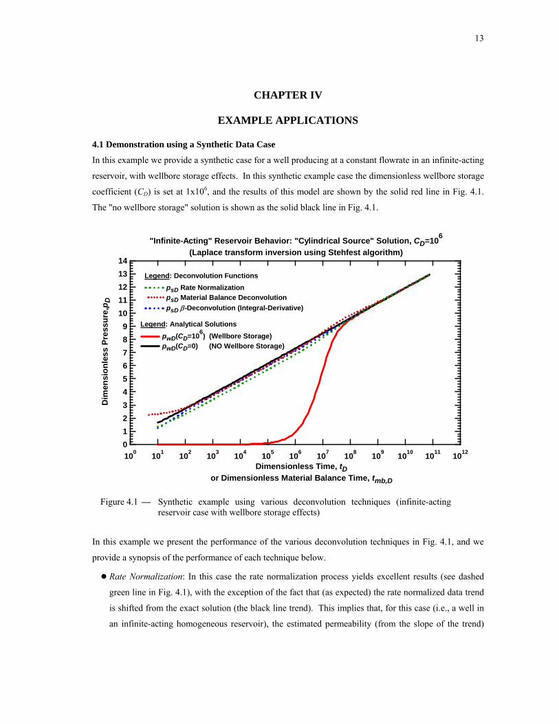
4.1 Demonstration using a Synthetic Data Case
In this example we provide a synthetic case for a well producing at a constant flowrate in an infinite-acting
reservoir, with wellbore storage effects. In this synthetic example case the dimensionless wellbore storage
coefficient (CD) is set at 1x10⁶, and the results of this model are shown by the solid red line in Fig. 4.1.
The "no wellbore storage" solution is shown as the solid black line in Fig. 4.1.
1413121110
9876543210
Dim
ensi
onle
ss P
ress
ure,
p D
100 101 102 103 104 105 106 107 108 109 1010 1011 1012
Legend: Analytical Solutions pwD(CD=106) (Wellbore Storage) pwD(CD=0) (NO Wellbore Storage)
"Infinite-Acting" Reservoir Behavior: "Cylindrical Source" Solution, CD=106
(Laplace transform inversion using Stehfest algorithm)
Legend: Deconvolution Functions
psD Rate Normalization psD Material Balance Deconvolution psD β-Deconvolution (Integral-Derivative)
Dimensionless Time, tDor Dimensionless Material Balance Time, tmb,D
Figure 4.1 — Synthetic example using various deconvolution techniques (infinite-acting reservoir case with wellbore storage effects)
In this example we present the performance of the various deconvolution techniques in Fig. 4.1, and we
provide a synopsis of the performance of each technique below.
Rate Normalization: In this case the rate normalization process yields excellent results (see dashed
green line in Fig. 4.1), with the exception of the fact that (as expected) the rate normalized data trend
is shifted from the exact solution (the black line trend). This implies that, for this case (i.e., a well in
an infinite-acting homogeneous reservoir), the estimated permeability (from the slope of the trend)
14
should be quite accurate — however; the skin factor (which is estimated from the intercept of the
pressure trend) will be in error. The level of error in the skin factor estimated from the rate
normalization technique will depend on the level of wellbore storage imposed on the system (more
wellbore storage, more error). The material balance deconvolution approach should resolve the error
in the skin factor as this approach provides a time correction as well as the pressure drop correction
provided by the rate normalization approach.
Material Balance Deconvolution: The material balance deconvolution technique performs extremely
well for this case, with only minor discrepancies at the start of the data set and at the point where the
wellbore storage and no wellbore storage solutions merge. This performance of this method is
excellent, and suggests that, based on the simplicity of the material balance deconvolution method,
this is probably the most practical approach for the analysis of pressure transient test data distorted by
wellbore storage.
β-Deconvolution: The β-deconvolution technique also performs very well for this case (surprisingly
well, in fact). This performance is most likely due to the analytic nature of the "data" (i.e., the
synthetic dimensionless pressure and auxiliary functions). In other words, the fact that we used the
analytical (i.e., exact) solutions in this process most likely accounts for the remarkable success of the
β-deconvolution technique for this example.
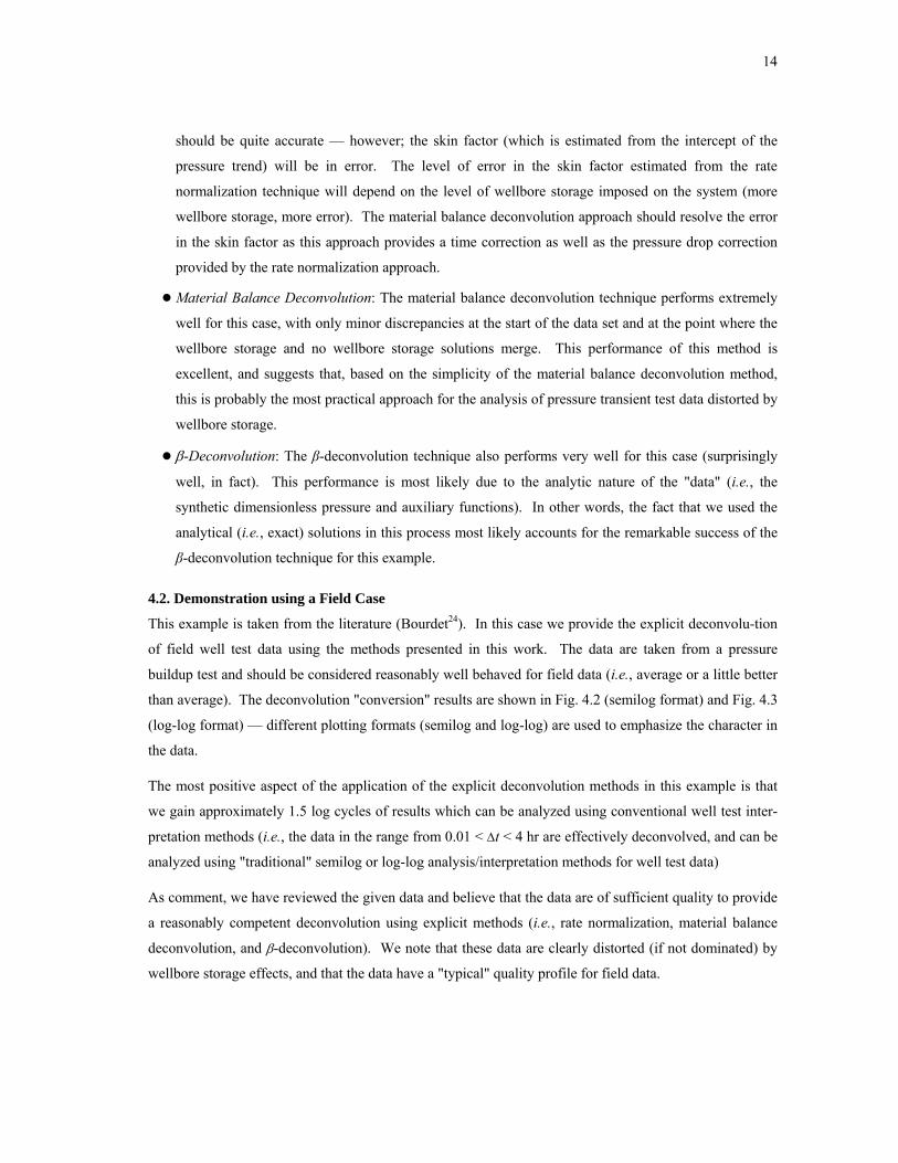
4.2. Demonstration using a Field Case
This example is taken from the literature (Bourdet24). In this case we provide the explicit deconvolu-tion
of field well test data using the methods presented in this work. The data are taken from a pressure
buildup test and should be considered reasonably well behaved for field data (i.e., average or a little better
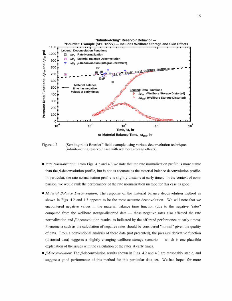
than average). The deconvolution "conversion" results are shown in Fig. 4.2 (semilog format) and Fig. 4.3
(log-log format) — different plotting formats (semilog and log-log) are used to emphasize the character in
the data.
The most positive aspect of the application of the explicit deconvolution methods in this example is that
we gain approximately 1.5 log cycles of results which can be analyzed using conventional well test inter-
pretation methods (i.e., the data in the range from 0.01 < ∆t < 4 hr are effectively deconvolved, and can be
analyzed using "traditional" semilog or log-log analysis/interpretation methods for well test data)
As comment, we have reviewed the given data and believe that the data are of sufficient quality to provide
a reasonably competent deconvolution using explicit methods (i.e., rate normalization, material balance
deconvolution, and β-deconvolution). We note that these data are clearly distorted (if not dominated) by
wellbore storage effects, and that the data have a "typical" quality profile for field data.
15
1100
1000
900
800
700
600
500
400
300
200
100
0
Pres
sure
Dro
p Fu
nctio
ns, ∆
p w a
nd ∆
p s, p
si
10-2 10-1 100 101 102
Legend: Data Functions ∆pw (Wellbore Storage Distorted) ∆pwd (Wellbore Storage Distorted)
"Infinite-Acting" Reservoir Behavior — "Bourdet" Example (SPE 12777) — Includes Wellbore Storage and Skin Effects
Legend: Deconvolution Functions
∆ps Rate Normalization ∆ps Material Balance Deconvolution ∆ps β-Deconvolution (Integral-Derivative)
Time, ∆t, hror Material Balance Time, ∆tmb, hr
Material balancetime has negative
values at early times
Figure 4.2 — (Semilog plot) Bourdet24 field example using various deconvolution techniques (infinite-acting reservoir case with wellbore storage effects)
Rate Normalization: From Figs. 4.2 and 4.3 we note that the rate normalization profile is more stable
than the β-deconvolution profile, but is not as accurate as the material balance deconvolution profile.
In particular, the rate normalization profile is slightly unstable at early times. In the context of com-
parison, we would rank the performance of the rate normalization method for this case as good.
Material Balance Deconvolution: The response of the material balance deconvolution method as
shown in Figs. 4.2 and 4.3 appears to be the most accurate deconvolution. We will note that we
encountered negative values in the material balance time function (due to the negative "rates"
computed from the wellbore storage-distorted data — these negative rates also affected the rate
normalization and β-deconvolution results, as indicated by the off-trend performance at early times).
Phenomena such as the calculation of negative rates should be considered "normal" given the quality
of data. From a conventional analysis of these data (not presented), the pressure derivative function
(distorted data) suggests a slightly changing wellbore storage scenario — which is one plausible
explanation of the issues with the calculation of the rates at early times.
β-Deconvolution: The β-deconvolution results shown in Figs. 4.2 and 4.3 are reasonably stable, and
suggest a good performance of this method for this particular data set. We had hoped for more

16
stability in the β-deconvolution at early times, but all of the explicit deconvolution methods were
affected at early times for this case and the β-deconvolution will not be immune to such effects.
101
102
103
104
Pres
sure
Dro
p Fu
nctio
ns, ∆
p w a
nd ∆
p s, p
si
10-2 10-1 100 101 102
Legend: Data Functions ∆pw (Wellbore Storage Distorted) ∆pwd (Wellbore Storage Distorted)
"Infinite-Acting" Reservoir Behavior — "Bourdet" Example (SPE 12777) — Includes Wellbore Storage and Skin Effects
Legend: Deconvolution Functions
∆ps Rate Normalization ∆ps Material Balance Deconvolution ∆ps β-Deconvolution (Integral-Derivative)
Time, ∆t, hror Material Balance Time, ∆tmb, hr
Material balancetime has negative
values at early times
Figure 4.3 — (Log-log plot) Bourdet24 field example using various deconvolution techniques (infinite-acting reservoir case with wellbore storage effects)
As closure commentary regarding this example, we believe that this example does indicate success for the
methods employed. Obviously the degree of success for any particular case will rely on the quality and
relevance of the data. As for a general recommendation, we encourage vigilance in data acquisition, and
care in the application of the methods used in this work. While these methods are theoretically supported,
these methods are highly susceptible to data errors and bias.
17
CHAPTER V
SUMMARY, CONCLUSIONS AND
RECOMMENDATIONS FOR FUTURE WORK
5.1 Summary and Conclusions
We summarize this work as follows — the expectation of success for the deconvolution of pressure
transient test data using explicit deconvolution techniques (rate normalization, material balance
deconvolution, and β-deconvolution) must be tempered with the knowledge that we create an inherent
bias when we do not use the rate profile — but rather, we infer the rate profile from a wellbore storage
model imposed (in some manner) on the pressure data.
Having made those qualifying comments, we should also recognize that the theory for each method does
provide confidence that these methods should perform well in practice. The primary concern must be the
quality and relevance of the pressure data. The following conclusions have been derived from this work:
Wellbore Storage Rate Models:
Governing relation(s): [mwbs = qB/(24Cs), where Cs is estimated from early time pressure data]
Pressure Drawdown Case:
wfiwf ppp −=∆ (5.1a)
][11, wfwbs
DDwbs pdtd
mq ∆−= (5.1b)
wfwbs
DDwbsDDwbsp pm
tdtqt
N ∆−== ∫ 1 0
,,, (5.1c)
Pressure Buildup Case:
)0( =∆−=∆ tppp wfwsws (5.2a)
][1, ws
wbsBUwbs p
tdd
mq ∆
∆= (5.2b)
wswbs
BUwbsBUwbsp pm
ttdqt
N ∆−∆=∆−∆
= ∫ 1 )1( 0
,,, (5.2c)
Conclusion(s):
Strength: Models are rigorous (based on consistent theory).
Weakness: Assumption of Cs = constant.

18
Rate Normalization:
Governing relation(s):
tvsq
p
DDwbs
wf . ,
∆ (pressure drawdown case) (5.3)
tvsq
p
BUwbsws ∆
−∆ .
1 , (pressure buildup case) (5.4)
Conclusion(s):
Strength: Rate normalization is a reasonably approximate correction.
Weakness: Pressure drop function is in error by a "shift" (i.e., a constant value).
Material Balance Deconvolution:
Governing relation(s):
DDwbs
DDwbsp
DDwbs
wfq
Nvs
qp
,
,,
, .
∆ (pressure drawdown case) (5.5)
BUwbs
BUwbsp
BUwbsws
qN
vsq
p
,
,,
, 1 .
1 −−∆ (pressure buildup case) (5.6)
Conclusion(s):
Strength: Very good correction, essentially best approximate method for practice.
Weakness: Slight "bump" in correction near end of wellbore storage trend (steep rate change).
β-Deconvolution:
Governing relation(s): (integral-derivative formulation for β(t) approximation)
widwdw
wdws p
ppppp ∆
∆−∆∆
+∆≈∆)(
(general — pressure drawdown or buildup case) (5.7a)
where:
dtpd
tp wwd
∆=∆ (pressure drawdown case) (5.7b)
tdpd
tp wwd ∆
∆∆=∆ (pressure buildup case) (5.7c)
dtpdtp wi
wid∆
=∆ where τdpt
tp wwi ∆=∆ ∫0
1 (pressure drawdown case) (5.7d)
td
pdtp wiwid ∆
∆∆=∆ where τdp
t
tp wwi ∆
∆
∆=∆ ∫0
1 (pressure buildup case) (5.7e)

19
β-Deconvolution: (continued)
Conclusion(s):
Strength: The "integral-derivative" formulation (Eq. 5.7a) appears to be most accurate.
Weakness: Erratic at very early times, also needs an exhaustive validation.
5.2 Recommendations for Future Work
The future work on this topic should consider mechanisms for further improvements in the material
balance deconvolution and β-deconvolution methods as these methods are applied to wellbore storage
distorted well test data.

20
NOMENCLATURE
Dimensionless Variables:
CD = dimensionless wellbore storage coefficient
tD = dimensionless time
pD = dimensionless pressure
qD = dimensionless rate Field Variables
Bo = oil formation volume factor, RB/STB
c = fluid compressibility, 1/psi
C2 = arbitrary constant, hr-1
h = net pay thickness, ft
k = formation permeability, md
mwbs = slope of wellbore storage dominated regime, psi/hr
Np = cumulative oil production, vol
p = reservoir pressure, psi
pwf(∆t=0) = wellbore pressure at the time of shut-in, psia
q = volumetric production rate, STB/D
r = radial distance, ft
s = skin factor
u = Laplace variable
t = producting time, hr
∆t = shut-in time, hr Greek
γ = Euler’s constant, γ ≈ 0.557216 …
β = "beta-deconvolution" variable, hr-1
µ = viscosity, cp
ρ = fluid density, lb/cuft Subscripts
a = after production period
d = "well-testing" derivative
D = dimensionless quantity
f = to pressure in the formation

21
i = initial reservoir conditions
i = "well-testing" pressure integral function
n = index number
w = conditions at wellbore radius Supercripts
' = derivative of a function
i = integral of a function
22
REFERENCES
1. Russell, D.G.: "Extensions of Pressure Build-Up Analysis Methods," paper SPE 1513 presented at the
1966 SPE Annual Meeting, Dallas, Texas, 2–5 October.
2. Gladfelter, R.E., Tracy, G.W., and Wilsey, L.E.: "Selecting Wells Which Will Respond to Production-
Stimulation Treatment," Drill. And Prod. Pract., API, Dallas (1955) 117–29.
3. Fetkovich, M.J., and Vienot, M.E.: "Rate Normalization of Buildup Pressure By Using Afterflow
Data," JPT (December 1984) 2211–24.
4. van Everdingen, A.F.: "The Skin Effect and Its Influence on the Productive Capacity of a Well,"
Trans., AIME (1953) 198, 171-76.
5. Hurst, W.: "Establishment of the Skin Effect and Its Impediment to Fluid Flow into a Well Bore," Pet.
Eng. (Oct. 1953) B6–B16.
6. Joseph, J.A., and Koederitz, L.F.: "A Simple Nonlinear Model for Representation of Field Transeint
Responses," paper SPE 11435, available from SPE, Richardson, Texas (1982).
7. Kuchuk, F.J.: "Gladfelter Deconvolution," paper SPE 16377 presented at the 1987 SPE California
Regional Meeting held in Ventura, California, 8–10 April.
8. Mattar, L., and Santo, M.: "How Wellbore Dynamics Affect Pressure Transient Analysis," J. Cdn.
Pet. Tech. (April 1992) 63-70.
9. van Everdingen, A.F., and Hurst, W.: "Application of the Laplace Transformation to Flow Problems
in Reservoirs," Trans., AIME (1949) 186, 305–24.
10. Agarwal, R.G., Al-Hussainy, R., and Ramey, H.J. Jr.: "An Investigation of Wellbore Storage and Skin
Effects in Unsteady Liquid Flow: I. Analytical Treatment," SPEJ (Sept. 1970) 278-290.
11. Wattenbarger, R.A., and Ramey, H.J. Jr.: "An Investigation of Wellbore Storage and Skin Effects in
Unsteady Liquid Flow: II. Finite Difference Treatment," SPEJ (Sept. 1970) 291-297.
12. Raghavan, R.: Well Test Analysis, Prentice Hall, Englewood Cliffs, New Jersey, 1993.
13. Ramey, H.J. Jr.:"Non-Darcy Flow and Wellbore Storage Effects in Pressure Build-up and Drawdown
of Gas Wells," Trans., AIME, (1965) 210, 223-233.
14. Hegeman, P.S., Hallford, D.L., and Joseph, J.A.: "Well-Test Analysis With Changing Wellbore
Storage", paper SPE 21829 presented at the SPE Rocky Mountain Regional/Low Permeability
Reservoirs Symposium in Denver, Colorado, April 15-17 1991.
23
15. Blasingame, T.A., Johnston, J.L., Lee, W.J., and Raghavan, R.: "The Analysis of Gas Well Test Data
Distorted by Wellbore Storage Using an Explicit Deconvolution Method," paper SPE 19099 presented
at the 1989 SPE Gas Technology Symposium, Dallas, TX, 07-09 June 1989.
16. Duhamel, J.M.C.: "Mémoire sur la méthode générale relative au mouvement de la chaleur dans les
corps solides plongés dans les milieux dont la température varie avec le temps," J. de Ec. Polyt.
(Paris) 14 (1833) 20-77.
17. Odeh, A.S. and Jones, L.G.: "Pressure Drawdown Analysis, Variable-Rate Case," Trans., AIME
(1965) 234, 960-64.
18. Agarwal, R.G.: "A New Method to Account for Producing Time Effects When Drawdown Type
Curves Are Used to Analyze Pressure Buildup and Other Test Data," paper SPE 9289 presented at the
1980 SPE Annual Technical Convention and Exhibition, Dallas, TX, 21 September-24 September.
19. Soliman, M.Y.: "New Technique for Analysis of Variable Rate or Slug Test," paper SPE 10083
presented at the 1981 SPE Annual Technical Convention and Exhibition, San Antonio, TX, 5-7
October.
20. Stewart, G., Wittmann, M.J., Meunier, D.: "Afterflow Measurement and Deconvolution in Well Test
Analysis," paper SPE 12174 presented at the 1983 Annual Technical Conference and Exhibition, San
Francisco, CA, 5-8 October.
21. Johnston, J.L.: “Variable Rate Analysis of Transient Well Test Data Using Semi-Analytical
Methods,” M.S. thesis, Texas A&M University, College Station, TX (1992).
22. Winestock, A.G., and Colpitts, G.P.: "Advances in Estimating Gas Well Deliverability," J. Cdn. Pet.
Tech. (July-Sept. 1965) 111–19.
23. Doublet, L.E., Pande, P.K., McCollum, T.J., and Blasingame, T.A.: "Decline Curve Analysis Using
Type Curves—Analysis of Oil Well Production Data Using Material Balance Time: Application to
Field Cases," paper SPE 28688 presented at the 1994 Petroleum Conference and Exhibition of Mexico
held in Veracruz, Mexico, October 10–13.
24. Bourdet, D., Ayoub, J.A., and Pirad, Y.M.: "Use of Pressure Derivative in Well-Test Interpretation,"
SPEFE (June 1989) 293-302 (SPE 12777).
25. Meunier, D., Wittmann, M.J., and Stewart, G.: "Interpretation of Pressure Buildup Test Using In-Situ
Measurement of Afterflow," JPT (January 1985), 143.
26. Abate, J., and Valkó, P.P.: "Multi-precision Laplace Transform Inversion" International Journal for
Numerical Methods in Engineering, 2004 v. 60, pp 979–993.

24
27. Ross, D., and Schoman, K.: "Structured Analysis for Requirements Definitions," IEEE Transactions
on Software Engineering 3(1), Special Issue on Requirements Analysis (Jan. 1977) 86-95.
25
APPENDIX A
RUSSELL METHOD FOR "CORRECTION" OF WELL TEST DATA
DISTORTED BY WELLBORE STORAGE (RUSSELL, 1966)
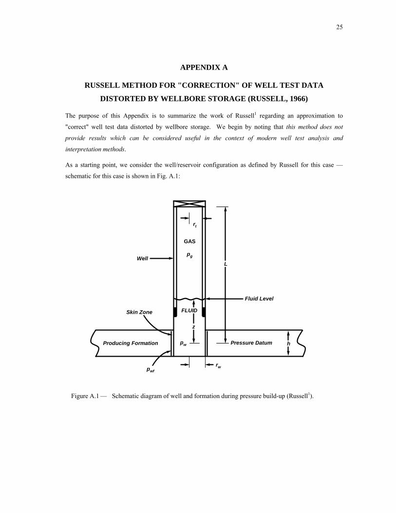
The purpose of this Appendix is to summarize the work of Russell1 regarding an approximation to
"correct" well test data distorted by wellbore storage. We begin by noting that this method does not
provide results which can be considered useful in the context of modern well test analysis and
interpretation methods.
As a starting point, we consider the well/reservoir configuration as defined by Russell for this case —
schematic for this case is shown in Fig. A.1:
h
L
rwpwf
z
GAS
pg
rt
Well
Fluid Level
FLUID
pwProducing Formation Pressure Datum
Skin Zone
Figure A.1 — Schematic diagram of well and formation during pressure build-up (Russell1).
26
Russell made the following assumptions in the derivation of his wellbore storage "correction" solution:
Completely penetrating well in an infinite reservoir.
Slightly compressible liquid (constant compressibility).
Constant fluid viscosity.
Single-phase liquid flow in the reservoir.
Gravity and capillary pressure neglected.
Constant permeability.
Horizontal radial flow (no vertical flow).
Ideal gas (for the gas cushion in the well).
Although the Russell method was derived from analytical considerations, the problem actually solved is a
variation of the true wellbore storage problem, derived using Russell's representation of the gas and liquid
volume in the wellbore as the "wellbore storage" term. This formulation is not based on the same physics
as the wellbore storage problem where the wellbore production (at the start of production or shut-in) is
inversely proportional to the compressibility of the fluids the wellbore (or the influence of a rising/falling
liquid level).
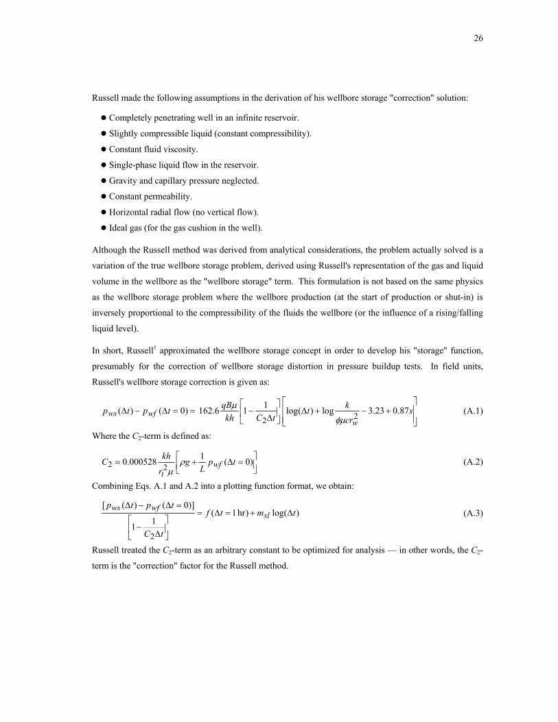
In short, Russell1 approximated the wellbore storage concept in order to develop his "storage" function,
presumably for the correction of wellbore storage distortion in pressure buildup tests. In field units,
Russell's wellbore storage correction is given as:
⎥⎥⎦
⎤
⎢⎢⎣
⎡+−+∆⎥
⎦
⎤⎢⎣
⎡∆
−==∆−∆ scrkt
tCkhqBtptp
wwfws 87.023.3log)(log 116.162 )0()( 22 φµ
µ (A.1)
Where the C2-term is defined as:
⎥⎦⎤
⎢⎣⎡ =∆+= )0(1000528.0 22 tp
Lg
r
khC wft
ρµ
(A.2)
Combining Eqs. A.1 and A.2 into a plotting function format, we obtain:
)(log)hr 1(11
)]0()([
2
tmtf
tC
tptpsl
wfws ∆+=∆=
⎥⎦
⎤⎢⎣
⎡∆
−
=∆−∆ (A.3)
Russell treated the C2-term as an arbitrary constant to be optimized for analysis — in other words, the C2-
term is the "correction" factor for the Russell method.
27
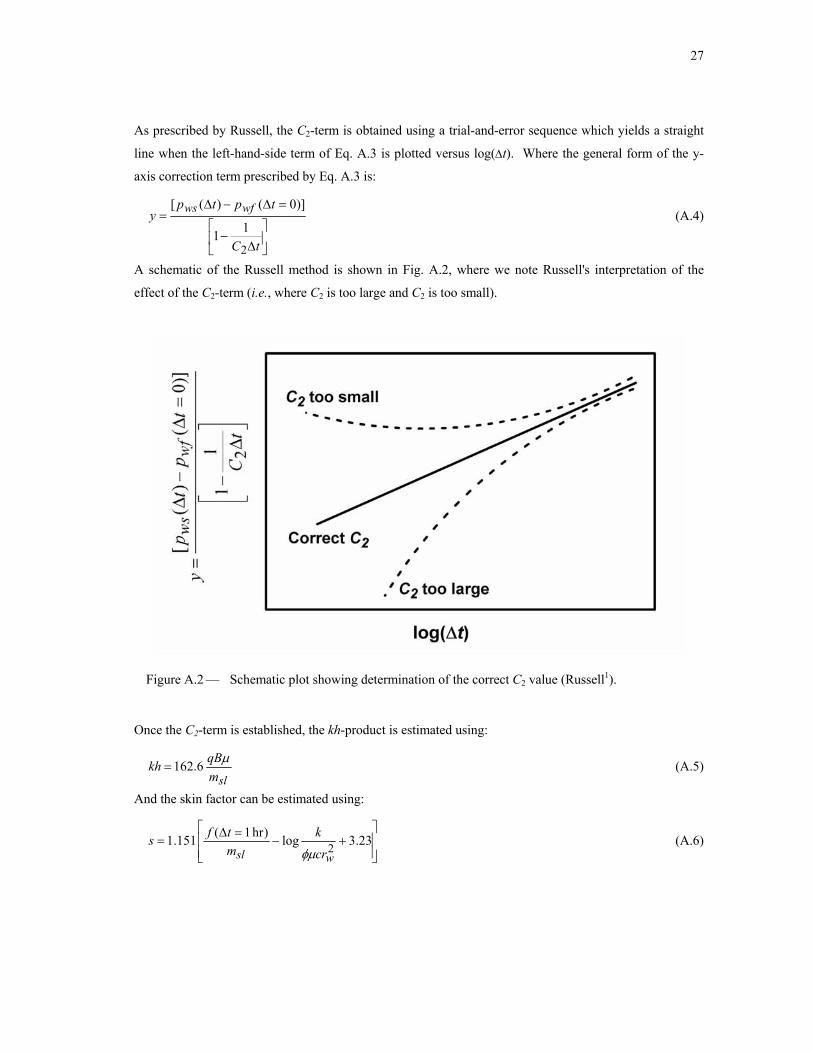
As prescribed by Russell, the C2-term is obtained using a trial-and-error sequence which yields a straight
line when the left-hand-side term of Eq. A.3 is plotted versus log(∆t). Where the general form of the y-
axis correction term prescribed by Eq. A.3 is:
⎥⎦
⎤⎢⎣
⎡∆
−
=∆−∆=
tC
tptpy wfws
2
11
)]0()([ (A.4)
A schematic of the Russell method is shown in Fig. A.2, where we note Russell's interpretation of the
effect of the C2-term (i.e., where C2 is too large and C2 is too small).
Figure A.2 — Schematic plot showing determination of the correct C2 value (Russell1).
Once the C2-term is established, the kh-product is estimated using:
slmqBkh µ 6.162= (A.5)
And the skin factor can be estimated using:
⎥⎥⎦
⎤
⎢⎢⎣
⎡+−
=∆= 23.3log)hr 1( 151.1 2
wsl crk
mtfs
φµ (A.6)
28
Russell1 also proposed a methodology to obtain the "extrapolated" pressure using the results of his
correction procedure. We chose not to demonstrate this methodology; the interested reader is referred to
Russell1 for more detail.
We present two example cases to demonstrate the shortcomings of the Russell method (lack of accuracy,
limited range of application). The first example is for "Well B," an example taken from the original
Russell reference [Russell1]. The second example is taken from data in the reference paper by Meunier, et
al.24.
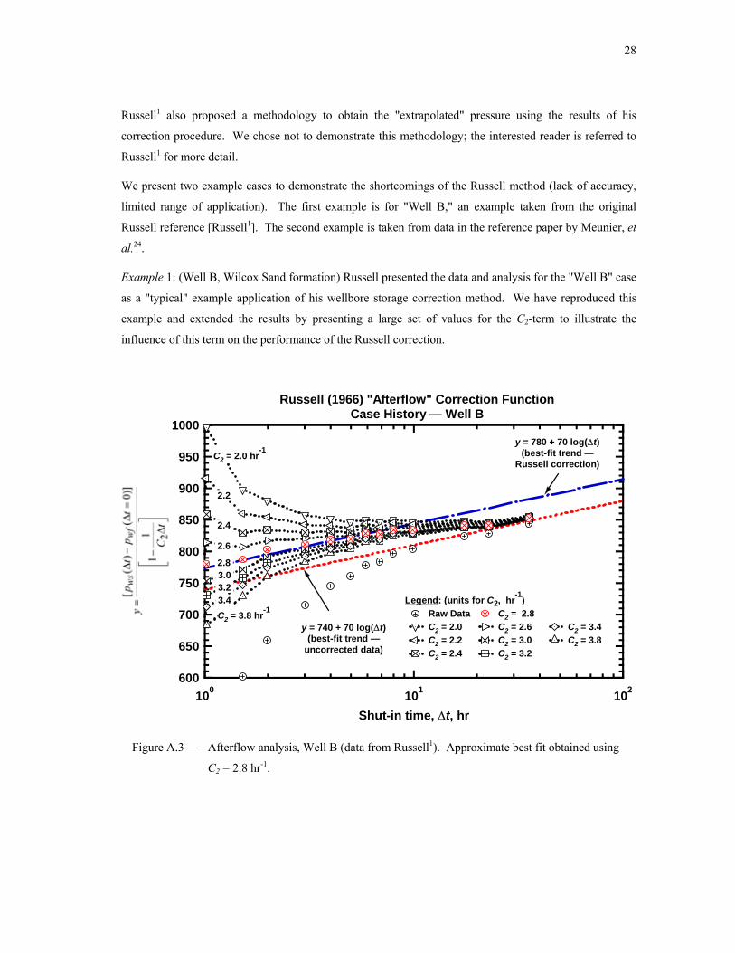
Example 1: (Well B, Wilcox Sand formation) Russell presented the data and analysis for the "Well B" case
as a "typical" example application of his wellbore storage correction method. We have reproduced this
example and extended the results by presenting a large set of values for the C2-term to illustrate the
influence of this term on the performance of the Russell correction.
1000
950
900
850
800
750
700
650
600100 101 102
Shut-in time, ∆t, hr
Legend: (units for C2, hr-1) Raw Data C2 = 2.8 C2 = 2.0 C2 = 2.6 C2 = 3.4 C2 = 2.2 C2 = 3.0 C2 = 3.8 C2 = 2.4 C2 = 3.2
Russell (1966) "Afterflow" Correction FunctionCase History — Well B
C2 = 2.0 hr-1
2.2
2.4
3.0 3.2 3.4
y = 740 + 70 log(∆t)(best-fit trend —
uncorrected data)
2.6
C2 = 3.8 hr-1
2.8
y = 780 + 70 log(∆t)(best-fit trend —
Russell correction)
Figure A.3 — Afterflow analysis, Well B (data from Russell1). Approximate best fit obtained using
C2 = 2.8 hr-1.
29
For our reproduction of this case, we use C2={2.0 2.4, 2.6, 2.8, 3.0, 3.2, 3.4, 3.8 hr-1} in Eq. A.4, and we
plot the results of this exercise on Fig. A.3. The value of the C2-term for which most of the points form a
straight line [y versus log(∆t)] is 2.8 hr-1, and we obtain a straight-line slope (msl) of about 70 psi/log cycle.
A comparison of our results and those obtained by Russell is shown below.
Conventional Analysis*
pws versus log(∆t)
Russell Correction Eq. A.4 versus
log(∆t) Analysis
msl (psi/log cycle)
msl (psi/log cycle)
Russell1 70 67 (C2=3.0 hr-1) This Study 70 70 (C2=2.8 hr-1)
* Conventional analysis based on using the pws vs. log(∆t) for data which are not affected by
wellbore storage effects. The "conventional" straight-line trend is constructed using the data in
the region of 10 < ∆t < 40 hours.
As shown in Fig. A.3, our selection of C2 = 2.8 hr-1 as the approximate best fit value appears to be the case
for which the Russell correction yields an apparent straight line trend. Russell1 noted that that C2=2.75 hr-1
"might well have been chosen instead [of 3.0]."

30
550
500
450
400
350
30010-1 100 101
Shut-in time, ∆t, hr
C2 = 11.9 C2 = 12.5 C2 = 13.5 C2 = 15.0
y = 436 + 53 log(∆t)(best-fit trend —
uncorrected data)
y = 476 + 53 log(∆t)(best-fit trend —
Russell correction)
Legend: (units for C2 hr-1) Pressure Drop C2 = 9.0 C2 = 10.0 C2 = 11.0 C2 = 11.5
C2 = 9.0 hr-1
11.9
10.0
11.5
11.0
12.513.5
C2 = 14.5 hr-1
Russell (1966) "Afterflow" Correction FunctionCase History — Meunier et al. (1985) Dataset
Figure A.4 — Afterflow analysis, Meunier et al.25 data set. Approximate "best" fit obtained using C2
= 11.9 hr-1.
Example 2: The following example is the field case given by Meunier et al.25. We have applied the
Russell "correction" method in this example and we used several values for the C2-term to illustrate the
influence of this term on the performance of the Russell correction. We use C2={9.0 10.0, 11.0, 11.5,
11.9, 12.5, 13.5, 14.5 hr-1} and we present our results in Fig. A.4. We obtained a slope value (msl) of about
53 psi/log cycle using the "best fit" value of the C2-term 11.9 hr-1.
In the analysis of Meunier et al.25, value of the slope was reported as 57 psi/log cycle using the "sandface
rate convolution" method.
If we consider the performance of the Russell method objectively as applied to the data of Meunier et al. 25, we would conclude that the "corrected" pressures (the symbols in Fig. A.4) are of little practical use.
Obviously such data could not be used for pressure derivative analysis — even if we could accept the
(very) approximate straight-line (i.e., the corrected data) such data would yield very erroneous pressure
derivative profiles.
31
APPENDIX B
DERIVATION OF THE β-DECONVOLUTION FORMULATION
We note that the lack of accuracy in flowrate measurements (when these exist) narrows the range of
application of Gladfelter deconvolution method (i.e., rate normalization). Van Everdingen4 and Hurst5
(separately) introduced an exponential model for the sandface rate during the wellbore storage distortion
period of a pressure transient test. The exponential formulation of the flowrate function is given as:
DtDD etq β−−= 1)( (B.1)
Eq. (B-1) is based on the empirical observations made by Van Everdingen and Hurst — and as extended
by others such as Kuchuk7 and Joseph and Koederitz6.
Recalling the convolution theorem, we have:
τττ dtpqt
tp DsD'D
DDwD )()(
0)( −= ∫ (B.2)
Taking the Laplace transform of Eq. B.2 yields:
)()()( upuquup sDDwD = (B.3)
Rearranging Eq. B.3 for the equivalent constant rate pressure drop function, )(upsD , we obtain:
)(1)()(
uquupup
DwDsD = (B.4)
The Laplace transform of the rate profile (Eq. B.1) is:
β+−=
uuuqD
11)( (B.5)
Substituting Eq. B.5 into Eq. B.4, and then taking the inverse Laplace transformation of this result yields
the "beta" deconvolution formula:
DDwD
DwDDsD dttdp
tptp)(1)()(
β+= (B.6)
Where we note that Eq. (B-6) is specifically valid only for the exponential sandface flowrate profile given
by Eq. B-1. This may present a serious limitation in terms of practical application of the β-deconvolution
method.
To alleviate the issue of the exponential sandface flowrate, we propose that Eq. B-6 be solved for the β-
term. Once this identity is established, we will then develop methods for estimating the β-term from data.

32
After that we will use the identity (Eq. B.6) to estimate the pressure drop function for a constant
production rate. Solving Eq. B.6 for the β-term, we have:
DDwD
DwDDsD dttdp
tptp)(
)()(1−
=β (B.7)
Or, multiplying through Eq. B.7 by the CD-term, we have
DDwD
DDwDDsD
D dttdp
Ctptp
C)(
)()(
1
−=β (B.8)
Recalling the definition of the wellbore storage model, we have:
DDwD
DDD dttdp
Ctq)(
1)( −= (B.9)
Assuming wellbore storage domination (i.e., qD ≈ 0) at early times, then Eq. B.9 becomes:
1)(
≈D
DwDD dt
tdpC (early time) (B.10)
Separating and integrating Eq. B.10 (our early time, wellbore storage domination result), we have:
DD
DwD Cttp ≈)( (early time) (B.11)
Substituting Eqs. B.10 and B.11 into Eq. B.8, we obtain:
DD
DsDD
Cttp
C−
=)(
1 β (early time) (B.12)
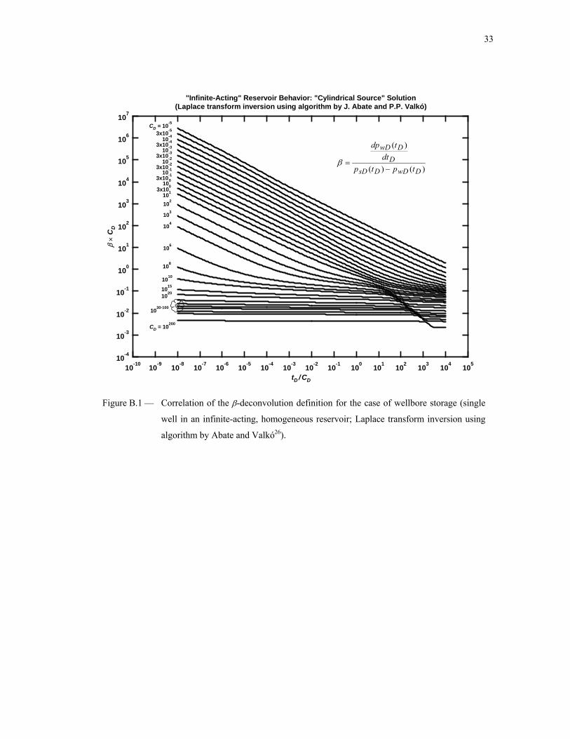
Eq. B.12 suggests that we can "correlate" the βCD product with tD/CD — this observation becomes the
basis for our use of these plotting functions to compare the β-deconvolution relations. The "master" plot
of the β-deconvolution function for the case of a single well in an infinite-acting, homogeneous reservoir
is derived using Eq. B.8 and is shown in Fig. B.1.
33
10-4
10-3
10-2
10-1
100
101
102
103
104
105
106
107β
× C
D
10-10 10-9 10-8 10-7 10-6 10-5 10-4 10-3 10-2 10-1 100 101 102 103 104 105
tD / CD
)()(
)(
DwDDsDD
DwD
tptpdt
tdp
−=β
CD = 10-5
3x10⁻⁵
10-4
3x10⁻⁴
3x10-310-3
10-2
3x10⁻²
10-1
3x10⁻¹
100
3x100
101
103
104
106
108
1010
1015
1020
1030-100
CD = 10200
102
"Infinite-Acting" Reservoir Behavior: "Cylindrical Source" Solution(Laplace transform inversion using algorithm by J. Abate and P.P. Valkó)
Figure B.1 — Correlation of the β-deconvolution definition for the case of wellbore storage (single
well in an infinite-acting, homogeneous reservoir; Laplace transform inversion using
algorithm by Abate and Valkó26).
34
APPENDIX C
DERIVATION OF THE COEFFICIENTS FOR β-DECONVOLUTION
C.1 β-Deconvolution — Derivative Approach
Although our stated goal is to develop a deconvolution approach which does not use the pressure
derivative function, we can at least develop such a methodology as it may be of practical use in the future.
Considering this problem only in terms of dimensionless solutions (and variables), we propose to use the
derivative of the pwD(tD) function as a mechanism to compute the rate function (in our case the β(tD)
function from the van Everdingen4 and Hurst5 exponential approximation for sand-face flowrate).
Recalling this exponential rate model, we have:
DD ttDD etq )(1)( β−−= (C.1)
Taking the time derivative of Eq. C.1 gives:
DD ttD
DD
DD etbdtdqtq )(' )()( β−== (C.2)
Where the b(tD)-term is defined as:
DDDD ttttb )(')()( ββ += (C.3)
Recalling the definition of the wellbore storage model, we have:
DwD
DDD dtdp
Ctq −= 1)( (C.4)
Taking the time derivative of Eq. C.4 gives:
)( ''2
2'
wDDD
wDD
DD
DD pCdt
pdC
dtdqtq −=−== (C.5)
Equating Eqs. C.2 and C.5 gives
DD ttD
D
wDDDwDD etb
dt
pdCtpC )(
2
2'' )()( β−−== (C.6)
Equating Eqs. C.1 and C.4 gives
)(')(DwDD
DwD
Dtt tpC
dtdp
Ce DD ==−β (C.7)

35
Combining Eqs. C.6 and C.7, and solving for b(tD)
DDD
wDdwDdd
D
wD
wDD
tttpp
t
p
ptb
)(')(
1
)( '
''
ββ +=
−=
−=
(C.8)
Where the pwDd and pwDdd terms are defined as:
DwD
DwDd dtdp
tp = (C.9)
2
22
D
wDDwDdd
dt
pdtp = (C.10)
We can use Eq. C.8 to determine β(tD) and β'(tD) — a graphical representation of this technique is shown
in Fig. C.1.
Figure C.1 — β-deconvolution via the derivative approach — β(tD) and β'(tD) determination.
The intercept and slope values [β(tD) and β'(tD), respectively] could be approximated by numerical
methods such as least squares — we do not suggest that this approach is functional, we simply present the
details for possible use in the future.
C.2 β-Deconvolution — Integral Approach
In this case, we assume β(tD) = β (constant) for the purposes of integration and differentiation. We will
use integrals and integral-difference (derivative) functions to estimate β(tD).
36
Recalling Eq. C.7, we have:
DD ttDwDD etpC )(' )( β−= (C.7)
Assuming β(tD) = β (constant), and integrating Eq. C.7 with respect to tD, we obtain
⎥⎦⎤
⎢⎣⎡ −= − DtDwDD etpC β
β11)( (C.11)
Integrating Eq. C.11 with respect to tD yields
⎥⎦
⎤⎢⎣
⎡⎥⎦⎤
⎢⎣⎡ −−= − DtDD
iwDD ettpC β
ββ111)( (C.12)
Where the )( DiwD tp function is given by:
ττ dpt
tp wDD
DiwD )(
0)( ∫= (C.13)
Substituting Eq. C.11 into Eq. C.12, we obtain
)]([1)( DwDDDDiwDD tpCttpC −=
β (C.14)
Dividing through Eq. C.14 by tD gives
⎥⎦
⎤⎢⎣
⎡−=
DDwD
DDwDiD ttpCtpC )(11)(
β (C.15)
Where the )( DwiD tp function in Eq. C.15 is given by:
ττ dpt
ttp wD
D
DDwDi )(
0
1)( ∫= (C.16)
Taking the derivative of Eq. C.15 with respect to tD yields:
⎥⎥
⎦
⎤
⎢⎢
⎣
⎡−−= 2
' )()()(
D
DwDD
DwDDD
DwDiD
t
tpt
tpCdt
tdpCβ
(C.17)
Dividing through by CD, and multiplying both sides by 2Dt
)]()([11)( DwDDwDdD
DwDid tptpt
tp −−=β
(C.18)
Where the )( DwDid tp function in Eq. C.18 is given by:
DDwDi
DDwDid dttdpttp )()( = (C.19)

37
10-4
10-3
10-2
10-1
100
101
102
103
104
105
106
107β
× C
D
10-10 10-9 10-8 10-7 10-6 10-5 10-4 10-3 10-2 10-1 100 101 102 103 104 105
tD / CD
)()(
)(
DwDDsDD
DwD
tptpdt
tdp
−=β
)(
)()(
DwDidDDwDdDwD
tpttptp −
=β
CD = 10-5
3x10⁻⁵
10-4
3x10⁻⁴
3x10-310-3
10-2
3x10⁻²
10-1
3x10⁻¹
100
3x100
101
103
104
106
108
1010
1015
1020
1030-100
CD = 10200
102
"Infinite-Acting"Reservoir Behavior: "Cylindrical Source" Solution(Laplace transform inversion using algorithm by J. Abate and P.P. Valkó)
Legend:
β calculated using (1) β calculated using (2): Integral approach
(1)
(2)
Figure C.2 — β-deconvolution via the integral-derivative approach (approximation of β using Eq. C-
20). (for wellbore storage effects in a single well in an in-finite-acting, homogeneous
reservoir; Laplace transform inversion using algorithm by Abate and Valkó26)
Solving Eq. C.18 for β gives us:
)()]()([1)(
DwDidDwDdDwD
DD tp
tptpt
t−
=≈ ββ (C.20)
Where we assume β ≈ βtD. Eq. C.18 is compared to the analytical formulation for β (Eq. B.7) in Fig. C.2
(βCD versus tD/CD) — and we note a very good correlation at "early" values of tD/CD (which is where
wellbore storage effects are most important).
Recasting Eq. C.20 into any consistent set of units, we have the following results for the "field units" form
of the β-parameter, which we will express as βf. The result for βf is.
widwdw
f ppp
t ∆∆−∆
=)(1β (pressure drawdown) (C.21a)
38
widwdw
f ppp
t ∆∆−∆
∆=
)(1β (pressure buildup) (C.21b)
Where the ∆pw, ∆pwd, ∆pwi, and ∆pwid functions are defined as:
wfiw ppp −=∆ (pressure drawdown) (C.22a)
)0( =∆−=∆ tppp wfwsw (pressure buildup) (C.22b)
dtpd
tp wwd
∆=∆ (pressure drawdown) (C.23a)
tdpd
tp wwd ∆
∆∆=∆ (pressure buildup) (C.23b)
τdpt
tp wwi ∆=∆ ∫0
1 (pressure drawdown) (C.24a)
τdpt
tp wwi ∆
∆
∆=∆ ∫0
1 (pressure buildup) (C.24b)
dtpd
tp wiwid
∆=∆ (pressure drawdown) (C.25a)
tdpd
tp wiwid ∆
∆∆=∆ (pressure buildup) (C.25b)
The ∆ps functions for the pressure drawdown and buildup cases are defined in field units as: (based on Eq.
B-6)
dtpd
pp wf
ws∆
+∆=∆β1 (pressure drawdown) (C.26a)
tdpd
pp wf
ws ∆∆
+∆=∆β1 (pressure buildup) (C.26b)
Substituting the for βf definitions (Eqs. C.21a and C.21b) into the appropriate ∆ps functions (Eqs. C.26a
and C.26b) gives the final "field" relation for β-deconvolution using the "integral-derivative" approach (a
single relation is obtained for both the pressure drawdown and pressure buildup cases).
widwdw
wdws
w
widwdw
ws
ppp
ppp
dtpd
ppp
t
pp
∆∆−∆
∆+∆=∆
∆
∆∆−∆
+∆=∆
)(or
)(1
1
(C.27)
39
APPENDIX D
MATERIAL BALANCE DECONVOLUTION RELATIONS FOR WELLBORE
STORAGE DISTORTED PRESSURE TRANSIENT DATA
Material balance deconvolution is an extension of the rate normalization method. Johnston21 defines a
new x-axis plotting function (material balance time) which provides an approximate deconvolution of the
variable-rate pressure transient problem. There are numerous assumptions associated with the "material
balance deconvolution" methods — one of the most widely accepted assumptions is that the rate profile
must change smoothly and monotonically. In practical terms, this condition should be met for the well-
bore storage problem.
The general form of material balance deconvolution is provided for the pressure drawdown case in terms
of the material balance time function and the rate-normalized pressure drop function. The material
balance time function is given as:
qN
t pmb = (D.1)
The rate-normalized pressure drop function is given by:
qpp
qp wfi )( −
=∆ (D.2)
The wellbore storage rate function for the pressure drawdown case, qwbs,DD, is given as:
][11, wfwbs
DDwbs pdtd
mq ∆−= (D.3)
The wellbore storage rate function for the pressure buildup case, qwbs,BU, is given as:
][1, ws
wbsBUwbs p
tdd
mq ∆
∆= (D.4)
Where the wellbore storage "slope" is defined as:
swbs C
qBm24
= (D.5)
And the pressure drop terms are defined as:
wfiwf ppp −=∆ (D.6)
)0( =∆−=∆ tppp wfwsws (D.7)

40
The wellbore storage cumulative production for the pressure drawdown case, Np,wbs,DD, is given as:
wfwbs
DDwbsDDwbsp pm
tdtqt
N ∆−== ∫ 1 0
,,, (D.8)
The wellbore storage cumulative production for the pressure buildup case, Np,wbs,BU, is given as:
wswbs
BUwbsBUwbsp pm
ttdqt
N ∆−∆=∆−∆
= ∫ 1 )1( 0
,,, (D-9)
The wellbore storage-based, material balance time function for the pressure drawdown case is given as:
][11
1
,
,,,
wfwbs
wfwbs
DDwbs
DDwbspDDmb
pdtd
m
pm
t
qN
t∆−
∆−==∆ (D.10)
The wellbore storage-based, rate-normalized pressure drop function for the pressure drawdown case is:
wfwf
wbsDDwbs
wfDDs p
pdtd
mq
pp ∆
∆−=
∆=∆
][11
1
,, (D.11)
The wellbore storage-based, material balance time function for the pressure buildup case is given as:
][11
1
1 ,
,,,
wswbs
wswbs
BUwbs
BUwbspBUmb
ptd
dm
pm
t
qN
t∆
∆−
∆−∆=
−=∆ (D.12)
The wellbore storage-based, rate-normalized pressure drop function for the pressure buildup case is:
wsws
wbsBUwbs
wsBUs p
ptd
dm
qpp ∆
∆∆
−=
−∆
=∆][11
11 ,
, (D.13)
Plotting the rate-normalized pressure function versus the material balance time function (on log (tmb)
scales) shows that the material balance time function does correct the erroneous shift in the semilog
straight-line obtained by rate normalization. We believe that the material balance deconvolution technique
is a practical approach (perhaps the most practical approach) for the explicit deconvolution of pressure
transient test data which are distorted by wellbore storage and skin effects.
41
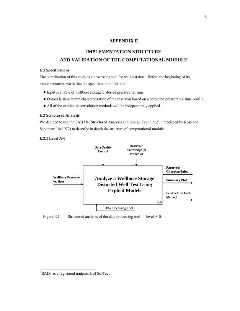
APPENDIX E
IMPLEMENTATION STRUCTURE
AND VALIDATION OF THE COMPUTATIONAL MODULE
E.1 Specifications
The contribution of this study is a processing tool for well test data. Before the beginning of its
implementation, we define the specification of this tool:
Input is a table of wellbore storage distorted pressure vs. time.
Output is an accurate characterization of the reservoir based on a corrected pressure vs. time profile.
All of the explicit deconvolution methods will be independently applied.
E.2 Structured Analysis
We decided to use the SADT® (Structured Analysis and Design Technique1, introduced by Ross and
Schoman27 in 1977) to describe in depth the structure of computational module.
E.2.1 Level A-0
A-0
Wellbore Pressure vs. time
Analyze a Wellbore Storage Distorted Well Test Using
Explicit Models
Reservoir Characteristics
Data Processing Tool
Reservoir Knowledge (if
available)
Feedback on Each Method
Summary Plot
Data Quality Control
A-0
Wellbore Pressure vs. time
Analyze a Wellbore Storage Distorted Well Test Using
Explicit Models
Reservoir Characteristics
Data Processing Tool
Reservoir Knowledge (if
available)
Feedback on Each Method
Summary Plot
Data Quality Control
Figure E.1 — Structured analysis of the data processing tool — level A-0.
1 SADT is a registered trademark of SofTech.
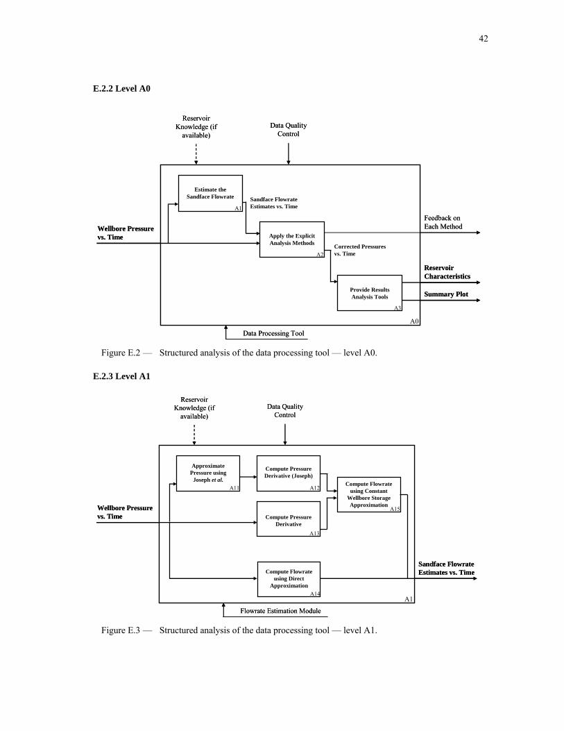
42
E.2.2 Level A0
A0
Wellbore Pressure vs. Time
Reservoir Characteristics
Data Processing Tool
Reservoir Knowledge (if
available)
Feedback on Each Method
Estimate the Sandface Flowrate
Apply the Explicit Analysis Methods
Summary Plot
Data Quality Control
Sandface FlowrateEstimates vs. Time
Provide Results Analysis Tools
Corrected Pressures vs. Time
A3
A2
A1
Figure E.2 — Structured analysis of the data processing tool — level A0.
E.2.3 Level A1
A1
Wellbore Pressure vs. Time
Flowrate Estimation Module
Reservoir Knowledge (if
available)
Approximate Pressure using
Joseph et al.
Compute Pressure Derivative
Sandface FlowrateEstimates vs. Time
Data Quality Control
Compute Flowrateusing Constant
Wellbore Storage Approximation
A13
Compute Pressure Derivative (Joseph)
A12
Compute Flowrateusing Direct
Approximation
A11
A14
A15
Figure E.3 — Structured analysis of the data processing tool — level A1.
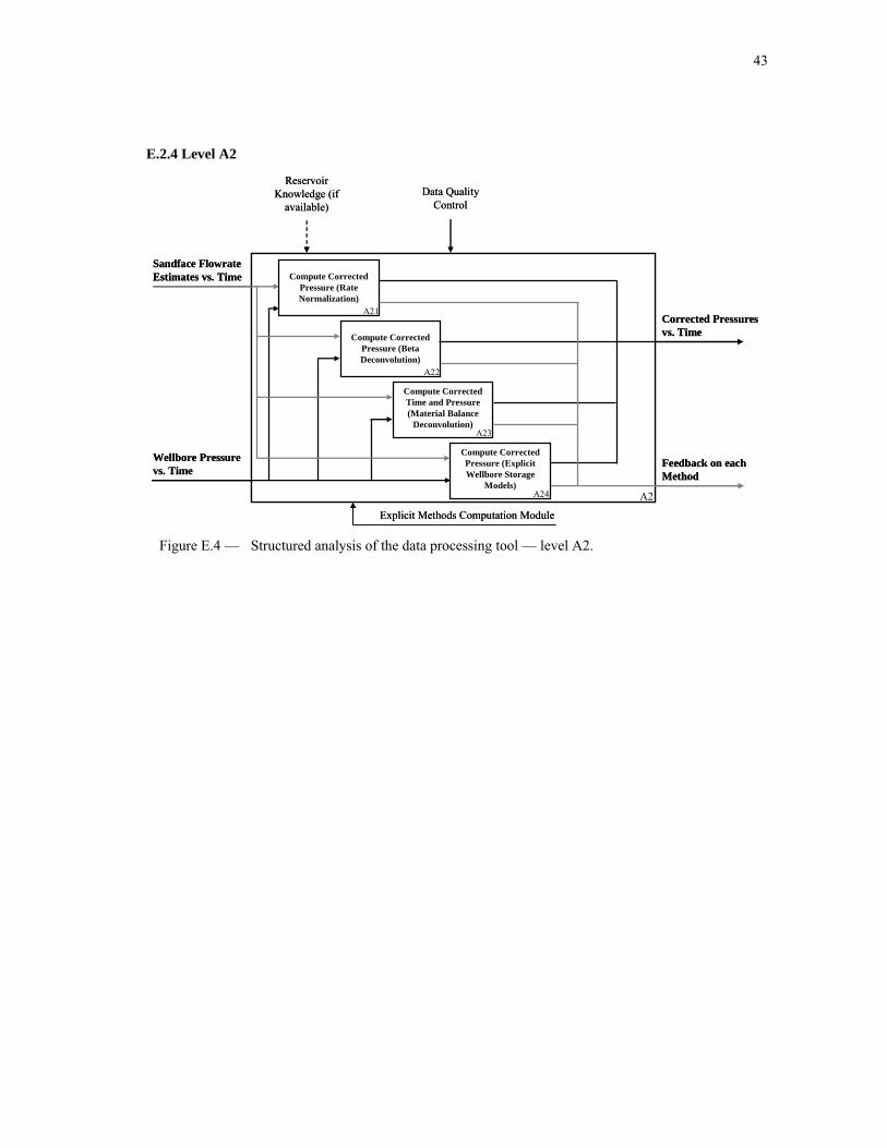
43
E.2.4 Level A2
A2
Wellbore Pressure vs. Time
Sandface FlowrateEstimates vs. Time
Corrected Pressures vs. Time
Explicit Methods Computation Module
Reservoir Knowledge (if
available)
Compute Corrected Pressure (Rate Normalization)
Data Quality Control
A21
A23
Compute Corrected Pressure (Beta Deconvolution)
A22
Compute Corrected Time and Pressure (Material Balance
Deconvolution)
A24
Compute Corrected Pressure (Explicit Wellbore Storage
Models)
Feedback on each Method
Figure E.4 — Structured analysis of the data processing tool — level A2.
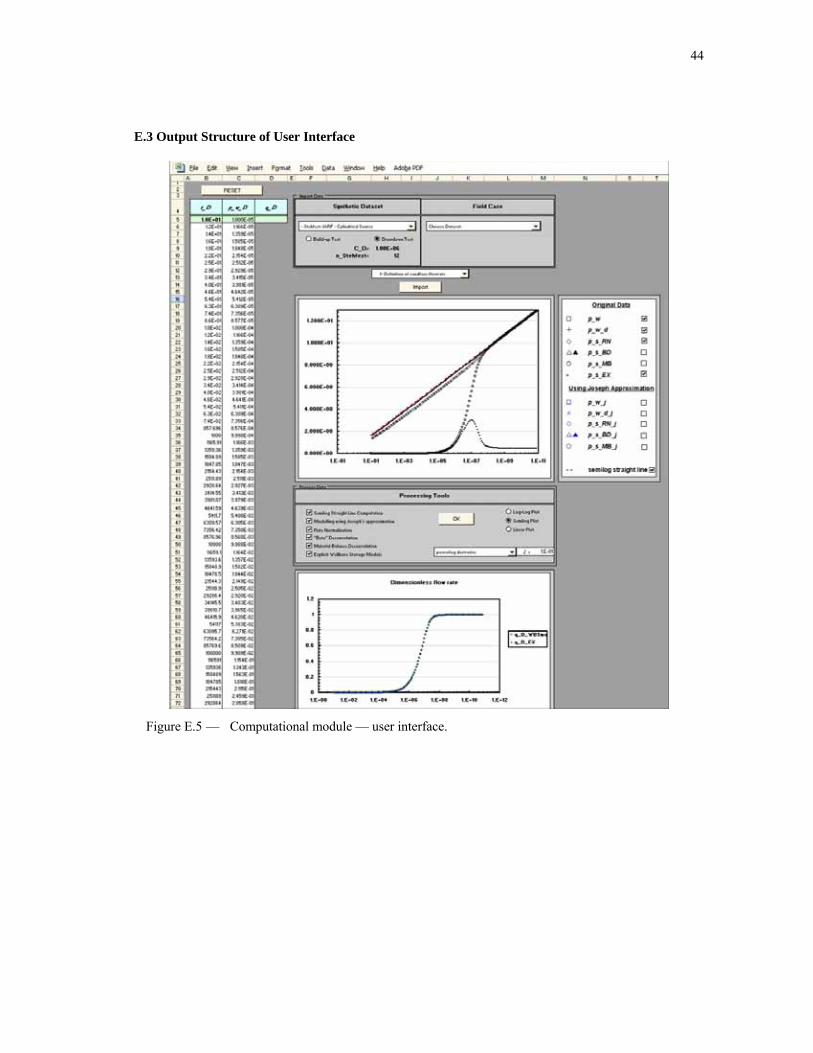
44
E.3 Output Structure of User Interface
Figure E.5 — Computational module — user interface.

45
VITA
Name: Olivier Bahabanian
Permanent Address: 1, route du Petit-Port-la-Claye
85400 Lairoux
France
E-mail Address: [email protected]
Education: Texas A&M University, College Station, Texas, USA
Master of Science Degree in Petroleum Engineering
December 2006
IFP School, Rueil-Malmaison, France
Master of Science Degree in Reservoir Geoscience and Engineering
August 2006
Ecole Nationale Supérieure des Mines, Paris, France
Diplôme d'Ingénieur Civil
July 2004
Affiliations: Society of Petroleum Engineers
Related Documents


