Explaining naïve Bayes classifications

1

Explaining Naïve Bayes Classifications

Duane Szafron [email protected]

Russell Greiner [email protected]

Paul Lu [email protected]

David Wishart [email protected]

Cam MacDonell [email protected]

John Anvik [email protected]

Brett Poulin [email protected]

Zhiyong Lu [email protected]

Roman Eisner [email protected] of Computing Science, University of AlbertaEdmonton AB T6G 2E8, Canada

AbstractNaïve Bayes classifiers, a popular tool for predicting the labels of query instances, are

typically learned from a training set. However, since many training sets contain noisy data, aclassifier user may be reluctant to blindly trust a predicted label. We present a novel graphicalexplanation facility for Naïve Bayes classifiers that serves three purposes. First, it transparentlyexplains the reasoning used by the classifier to foster user confidence in the prediction. Second, itenhances the user's understanding of the complex relationships between the features and the labels.Third, it can help the user to identify suspicious training data. We demonstrate these ideas in thecontext of our implemented web-based system, which uses examples from molecular biology.

1. IntroductionClassifiers are now being used by a variety of scientists to solve a wide range of computational problems.For example, bioinformaticians routinely use classifiers to predict properties of the thousands of new DNAsegments being sequenced every day. Each classifier maps a large set of sequence features to a predictedlabel representing a property of the sequence, such as general function or sub-cellular localization. However,in many cases, scientists may be reluctant to accept classification results without an explanation (Teach &Shortliffe 1984). For example, if a classifier is a "black box" and predicts that a query sequence is in theclass of transport/binding proteins without providing some justification, a scientist may not have muchconfidence in the prediction, even if the scientist agrees with the classifier. A worse situation is if thescientist disagrees with the prediction that a classifier has made for a particular sequence, but is given noinsight into why the classifier made this choice. In that situation, the scientist may distrust the classifieritself and not just the specific prediction. A good explanation not only helps to reinforce an accurateprediction, it also elucidates an inaccurate prediction in a way that identifies the location in the classifier’sreasoning where mis-information or lack of information caused the inaccuracy. In such a situation, theclarity of the explanation maintains, and often extends, the scientist’s overall confidence in the classifier.

We feel that a successful explanation must appeal to the scientist's intuition and must be able to answerthe most common prediction questions. In essence, this makes the classifier more of a “white-box”technique. Towards that goal, we have focused our efforts on Naïve-Bayes (NB) classifiers because they arebased on well-known probability concepts, which are generally understood by scientists. This is in contrastto other classifier techniques, such as Support Vector Machines (SVM) and Artificial Neural Networks(ANN), that may in some circumstances be more accurate than NB, but lack this intuitive basis. We havedeveloped a technique to present our explanations to non-computational scientists in an intuitive graphical(pictorial) format. We have defined a series of explanation capabilities ordered by increasing level of detail,to answer the common questions in the order that they are usually asked: What is the most likelyclassification and how "close" are the other possible classes? What specific evidence contributed to the

2

classification decision? When the evidence supported more than one class, how was the evidence weighedto obtain the final classification? What is the source of the basic evidence and how does that evidencerelate to the specific training set used to build the classifier? What are the application-specificcomputational techniques that were used to transform basic data to features?

1.1 Related WorkThe term explanation has several meanings, especially in the context of Bayesian inference. We aredescribing a process (and a system) to help explain the results of a particular classification or prediction, interms of both the particular query instance provided, and the data sample used to generate this model. Thisfits clearly as one task in the Lacave and Diez (2000) trichotomy as LD-3 – explanation of reasoning, sinceit explains why the classifier returned its specific answer to a query instance.

Our process also addresses another task, LD-2 – explanation of the model, as it relates to the staticmodel of the underlying NB belief net. Our approach differs from most LD-2 task systems, since we donot use this explanation to help justify the NB structure. However, our system does describe how thetraining data affects the parameters of the model, as a way to consider what training data may be suspect,and perhaps cause the model to produce a problematic classification.

Our process does not address one LD task, LD-1 – explanation of the evidence, which corresponds tofinding the most probable explanation (MPE). Finally, we are not trying to explain the general idea ofBayesian reasoning, nor Bayesian belief networks (Myllymäki et al. 2002).

1.2 BackgroundTo explain the context for our process, we first describe NB systems in general, and show how theirparameters are estimated from a data sample. In general, classifiers describe each instance using a set offeature-value pairs

†

F1,vk1( )... Fm ,vkm( ). Probabilistic classifiers typically return the label

†

L j with the largest

posterior probability,

†

Pj* = P L = L j | F1 = vk1

,...Fm = vkm[ ] . In this paper, we consider NB classifiers, which

make the simplifying assumption that the features are independent of each other, given the label (Duda &Hart 1973); see Equation 1.

Any NB classifier can be described by a set of parameters, which are typically learned from labeledtraining data (Heckerman 1998). We let

†

cijki denote the number of training instances labeled by

†

L j , whose

value for feature

†

Fi is

†

vki and call them the information atoms. We can derive the quantities:

†

n j (number

of training instances labeled by

†

L j ) and n (total number of training instances) from these information

atoms. Given the NB assumption, we can derive a formula for each posterior probability,

†

Pj* and define its

maximum likelihood estimator,

†

ˆ P j , in terms of the

†

cijki, where the normalization constant

†

a = P F1 = vk1,...Fm = vkm[ ] ensures that the probabilities add to 1, as shown in Equation 1.

†

Pj* = P L = L j | F1 = vk1

,...,Fm = vkm[ ] =

P L = L j[ ] ¥ P Fi = vki| L = L j[ ]

i=1

m

’

P F1 = vk1,...,Fm = vkm[ ]

ˆ P j =1a

n j

nÊ

Ë Á

ˆ

¯ ˜

cijki

n j

Ê

Ë Á Á

ˆ

¯ ˜ ˜

i=1

m

’

(1)

A classification explanation is a presentation of the evidence used by the classifier to assign eachprobability. Note that we use the term evidence to refer to the way that the information atoms,

†

cijki, are

used to make a classification. We are not referring to the evidence in the posterior distribution,

†

Fi = vki[ ].We address the challenge of effectively displaying this evidence for each query instance probability, using

3

the information atoms. A good explanation should present the evidence in a way that clearly establishes alink between the information atoms and the computed probabilities. In a non-graphical approach, this couldbe provided by a sequence of inferences that explain the factors in Equation 1. However, our goal is toderive an intuitive graphical explanation facility that can be used by scientists who have a basicunderstanding of probabilities, but may not have significant computational knowledge.

In this paper, the terms graph and graphical denote pictorial representations and are not used in themathematical sense of an entity consisting of vertices and edges. For presentation simplicity, we assumeeach feature has two domain values, denoting the presence of some token. We use Fi=1 when theassociated token is present, and Fi=0 when it is absent. However, the results are applicable to the generalcase, when each feature has a finite domain.

1.3 Example – Proteome AnalystWe use a NB classifier built for the Proteome Analyst (PA) web-based application(www.cs.ualberta.ca/~bioinfo/PA) (Szafron et al. 2003) as an example in this paper. This is a real classifierwith 2539 training instances and 1259 different features. It is used by molecular biologists and the queryinstance used in this paper is also real. It is the protein ATKB_Ecoli. However, we show only 8 of the 14labels to avoid distracting the reader with irrelevant details. Note that no knowledge of molecular biologyis required to understand this example, since the features and labels can be viewed as text strings.

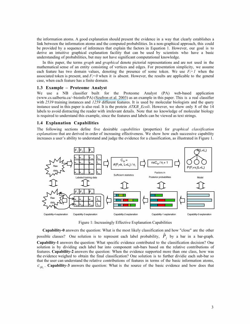
1.4 Explanation CapabilitiesThe following sections define five desirable capabilities (properties) for graphical classificationexplanations that are derived in order of increasing effectiveness. We show how each successive capabilityincreases a user’s ability to understand and judge the evidence for a classification, as illustrated in Figure 1.

Figure 1: Increasingly Effective Explanation Capabilities

Capability-0 answers the question: What is the most likely classification and how "close" are the other

possible classes? One solution is to represent each label probability,

†

ˆ P j by a bar in a bar-graph.

Capability-1 answers the question: What specific evidence contributed to the classification decision? Onesolution is by dividing each label bar into component sub-bars based on the relative contributions offeatures. Capability-2 answers the question: When the evidence supported more than one class, how wasthe evidence weighed to obtain the final classification? One solution is to further dividie each sub-bar sothat the user can understand the relative contributions of features in terms of the basic information atoms,

†

cijki. Capability-3 answers the question: What is the source of the basic evidence and how does that

P(L=Lj)

P(Fj=vij|L=Lj)

Capability-0 explanation

Rawdata

Labeled training data

v11 v12 … v1m

v21 v22 … v2m

… … … …vn1 vn2 … vnm

L1

L1

Lq

…

F1 F2 … Fm

Cijk =#(Fi=k, L=Lj) / ni

Sufficient statistics

nxCijk / ni + 1

Factors inPosterior probabilities Model

Capability-1 explanationCapability-2 explanationCapability-3 explanationCapability-4 explanation

v11 v12 … v1m

v21 v22 … v2m

L1

L1

F1 F2 … Fm

Rawdata

4

evidence relate to the specific training set used to build the classifier? One solution is to allow the to viewfeature information in the context of training data. Capability-4 answers the question: What are theapplication-specific computational techniques that were used to transform basic data to features? A solutionmust allow the user to view the relationship between raw training data and labeled feature lists.

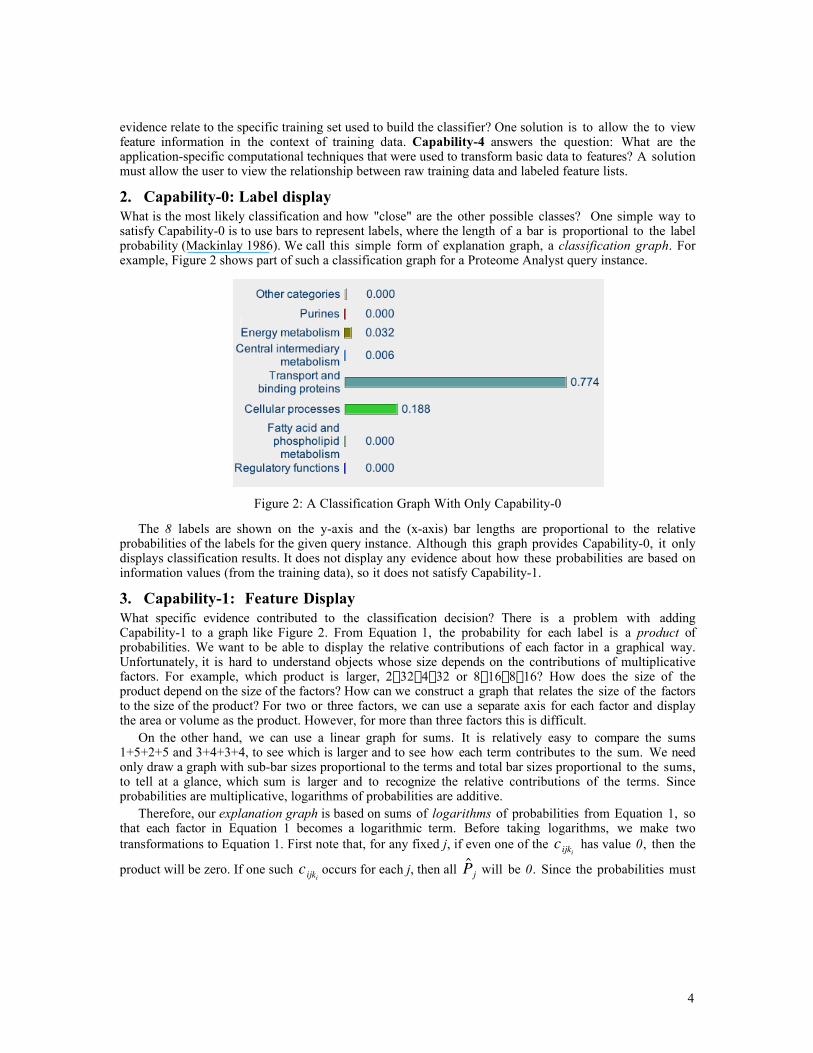
2. Capability-0: Label displayWhat is the most likely classification and how "close" are the other possible classes? One simple way tosatisfy Capability-0 is to use bars to represent labels, where the length of a bar is proportional to the labelprobability (Mackinlay 1986). We call this simple form of explanation graph, a classification graph. Forexample, Figure 2 shows part of such a classification graph for a Proteome Analyst query instance.

Figure 2: A Classification Graph With Only Capability-0

The 8 labels are shown on the y-axis and the (x-axis) bar lengths are proportional to the relativeprobabilities of the labels for the given query instance. Although this graph provides Capability-0, it onlydisplays classification results. It does not display any evidence about how these probabilities are based oninformation values (from the training data), so it does not satisfy Capability-1.

3. Capability-1: Feature DisplayWhat specific evidence contributed to the classification decision? There is a problem with addingCapability-1 to a graph like Figure 2. From Equation 1, the probability for each label is a product ofprobabilities. We want to be able to display the relative contributions of each factor in a graphical way.Unfortunately, it is hard to understand objects whose size depends on the contributions of multiplicativefactors. For example, which product is larger, 2¥32¥4¥32 or 8¥16¥8¥16? How does the size of theproduct depend on the size of the factors? How can we construct a graph that relates the size of the factorsto the size of the product? For two or three factors, we can use a separate axis for each factor and displaythe area or volume as the product. However, for more than three factors this is difficult.

On the other hand, we can use a linear graph for sums. It is relatively easy to compare the sums1+5+2+5 and 3+4+3+4, to see which is larger and to see how each term contributes to the sum. We needonly draw a graph with sub-bar sizes proportional to the terms and total bar sizes proportional to the sums,to tell at a glance, which sum is larger and to recognize the relative contributions of the terms. Sinceprobabilities are multiplicative, logarithms of probabilities are additive.

Therefore, our explanation graph is based on sums of logarithms of probabilities from Equation 1, sothat each factor in Equation 1 becomes a logarithmic term. Before taking logarithms, we make twotransformations to Equation 1. First note that, for any fixed j, if even one of the

†

cijki has value 0, then the

product will be zero. If one such

†

cijkioccurs for each j, then all

†

ˆ P j will be 0. Since the probabilities must

5

still add to 1, the normalization constant a must also be 0 so that Equation 1 becomes indeterminate (zerodivided by zero). Since this occurs frequently in practice, there are standard approaches to deal with thisproblem. The simplest solution is to use a Laplacian correction (Lidstone 1920) to construct a differentestimator,

†

˜ P j . Each factor in the product is replaced by a factor that cannot be zero as shown in Equation

2. The value

†

di is the number of distinct values that can be assigned to feature

†

Fi . In this paper,

†

di = 2for all i, since each feature is Boolean (absence or presence of a token). This is also a standard variance-reduction technique (Ripley 1996), with an obvious Bayesian MAP interpretation.

†

ˆ P j =1a

n j

nÊ

Ë Á

ˆ

¯ ˜

cijki

n j

Ê

Ë Á Á

ˆ

¯ ˜ ˜

i=1

m

’

˜ P j =1a

n j

nÊ

Ë Á

ˆ

¯ ˜

cijki+1

n j + di

Ê

Ë Á Á

ˆ

¯ ˜ ˜

i=1

m

’(2)

There are many variations of this technique (Ristad 1995) and we chose to reduce the bias of this basicestimator by instead using the formula in Equation 3, to define a new estimator,

†

Pj . Recall that

†

n j is the

number of training instances labeled by

†

L j and n is the total number of training instances. Therefore

†

n j

nis strictly less than 1, since if there is only 1 label, the classifier is useless. Also,

†

n j must be larger than

0, since any label without at least one training instance can never be predicted by the classifier and cantherefore be excluded.

†

Pj =1a

n j

nÊ

Ë Á

ˆ

¯ ˜

cijki+

n j

nn j + di ¥

n j

n

Ê

Ë

Á Á Á

ˆ

¯

˜ ˜ ˜ i=1

m

’ (3)

Before taking the logarithms in Equation 3, we make a transformation to this estimator. As each factorin Equation 3 is a probability, it is less than one. Since we will represent the logarithm of each factor as abar in a graph, we want each factor to be greater than or equal to 1, so that its logarithm will be non-negative. Therefore, we multiply each of the m factors by n and compensate by dividing the product by

†

nm . We then simplify the result to obtain Equation 4, where a’ is a new normalization constant.

†

Pj =1a

n j

nm +1

Ê

Ë Á

ˆ

¯ ˜

n ¥ cijki+ n j

n ¥ n j + di ¥ n j

Ê

Ë Á Á

ˆ

¯ ˜ ˜

i=1

m

’ =n j

a 'nn j

Ê

Ë Á Á

ˆ

¯ ˜ ˜ ¥ cijki

+1È

Î Í Í

˘

˚ ˙ ˙ i=1

m

’

where a '= a ¥ nm +1 n + di( )i=1

m

’(4)

Finally, we can take the logarithm of both sides of Equation 4 to obtain Equation 5. Each of thelogarithmic terms in the summation is non-negative since its argument is larger than or equal to 1.

†

log Pj( ) = log cijki¥

nn j

Ê

Ë Á Á

ˆ

¯ ˜ ˜ +1

È

Î Í Í

˘

˚ ˙ ˙ i=1

m

 + log n j( ) - log a '( ) (5)

6

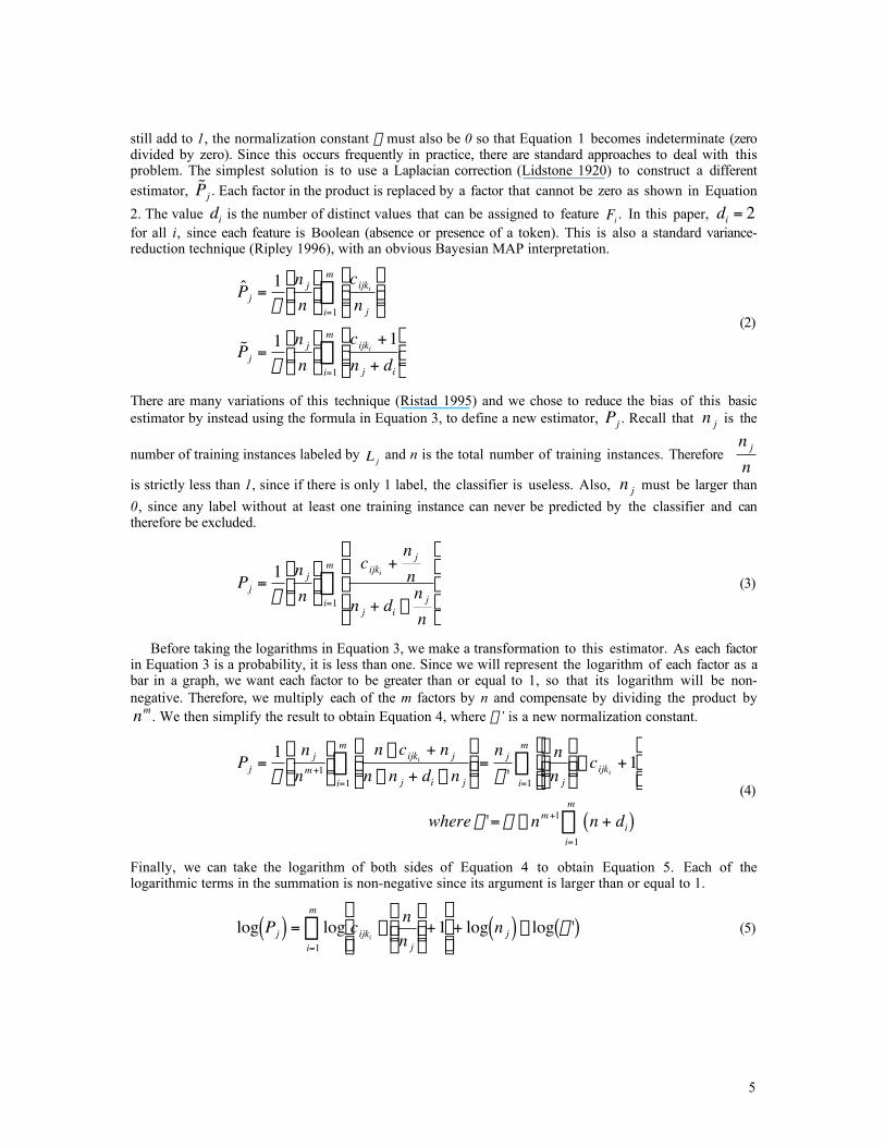
We will use the Proteome Analyst explanation graph shown in Figure 3 as an example. The queryinstance contained the nine features: atp-binding, ipr001454, transmembrane, inner membrane,phosphorylation, magnesium, potassium transport, ipr001757 and hydrolase. Similar to a classificationgraph, each of the eight labels is represented by a horizontal bar.

Figure 3: An Explanation Graph With Feature Sub-bars to Support Capability-1

However, there are two major differences between the Capability-0 classification graph (Figure 2) andthe Capability-1 explanation graph (Figure 3). First, the explanation graph has bars with lengthsproportional to the logarithms of probabilities of the labels. How can we use these lengths to compareprobabilities in order to maintain Capability-0?

We begin by defining the total gain of label Lj over label Lh as a measure of the preference of aprediction for one label over another, as shown in Equation 6.

†

G jhT = log Pj( ) - log Ph( ) (6)

We can use the total gain to compute the ratio of probabilities of the two labels as shown in Equation 7.

†

Pj

Ph

= 2log

Pj

Ph

Ê

Ë Á

ˆ

¯ ˜

= 2log Pj( )- log Ph( ) = 2G jhT

(7)

For example, in Figure 3, the longest bar is for the favorite label (largest probability), Transport andbinding proteins (TBP) with length approximately 45. The second longest bar is for the contender label(second largest probability), Cellular processes (CP) with length approximately 43. Applying Equation 7yields Equation 8.

†

PTBP

PCP

ª 2log 45( )- log 43( ) = 22 = 4 (8)

In fact, the predicted probabilities are 0.774 and 0.188, which have a probability ratio of 4.14. Since thescale is logarithmic, small differences in the logarithms of probabilities translate into large ratios ofprobabilities. Nevertheless, Capability-0 is satisfied.

7

To show Capability-1 compliance, we first decompose each bar in into sub-bars called: feature sub-bars, residual sub-bars and prior sub-bars, corresponding to terms from Equation 5 that are called featureterms, residual terms and prior terms respectively.

3.1 Feature termsFrom Equation 5, we can see that each feature Fi contributes to the probability that the query sequence haslabel Lj by an amount we call a feature term defined by Equation 9.

†

Fij = log cijki¥

nn j

Ê

Ë Á Á

ˆ

¯ ˜ ˜ +1

È

Î Í Í

˘

˚ ˙ ˙

(9)

To represent this information value in an explanation graph, we display a feature sub-bar. The feature sub-bar for label Lj has length proportional to the feature term, Fij. For this paper, we have annotated some ofthe sub-bars in Figure 3 with symbols (a) to (m). For example, from Figure 3, the feature sub-bar (f) ofinner membrane for label TBP has length 8.1. To use this length in a meaningful way, we must compare itto the length of another sub-bar in the graph.

We define the feature gain of a feature Fi relative to the labels Lj and Lh as a measure of how much thisfeature contributes to the probability of one label over the other, as given by Equation 10.

†

GijhF = Fij - Fih (10)

A positive feature gain gives positive evidence for the first label over the second. Otherwise it givesnegative evidence. For example, in Figure 3, the feature gain of inner membrane for label TBP over labelCP is the difference in lengths of the two sub-bars, (f) and (j). This gain of 8.1 - 5.4 = 2.7 is significantsince the difference in total lengths of the TBP bar and the CP bar is only 2.

Since the number of features can be large, we display sub-bars for only a subset of features called thefocus features. Features whose sub-bars are not explicitly displayed are called non-focus features. Forexample, Figure 3 has five focus features: potassium transport, ipr001757, ipr001454, inner membraneand magnesium. All other 1254 features are non-focus features. In Section 3.4, we describe how the defaultfocus features are selected, and present a mechanism for the user to change the focus features.

In general, not every focus feature will provide positive evidence for the predicted label over all otherlabels. For example, from Figure 3, the feature gain of ipr001757 relative to the labels TBP (sub-bar e) andCP (sub-bar i) is 4.2 - 5.2 = -1.0. Therefore, this feature gives negative evidence for the predicted label.Ultimately, the gain of any single feature is not important, only the total gain.

3.2 Residual TermThe focus feature sub-bars represent only a few of the feature terms shown in Equation 9. The non-focusfeature terms are combined into a residual term defined by Equation 11.

†

R j = Fijiœ focusfeatures{ }

 (11)

A residual sub-bar is added to the graph with length proportional to the residual term. However, in the PAexample (and any other application with a large number of features), the number of features in the residualis usually much larger than the number of focus features. Therefore, even though the size of each individualfeature included in the residual sub-bar is small, the total size of the residual sub-bar would often dwarf thesize of the focus feature sub-bars. To allow the user to clearly see the relative contributions of the focusfeatures, we subtract the length of the shortest residual term from all the residual terms to obtain thereduced residual term defined in Equation 12.

8

†

ˆ R j = R j - minh=1..q

Rh{ } (12)

Since only the difference of the bars is used to compute the ratio of probabilities, this effectively zoomsin on the focus features. For example, in Figure 3, the length of the residual sub-bar (a) for the first labelOther categories (OC), is zero, since its residual term is the smallest and this term was subtracted from allthe residual terms.

To compare residual terms across labels, we define the residual gain relative to the labels Lj and Lh byEquation 13.

†

G jhR = R j - Rh = ˆ R j - ˆ R h (13)

For example, in Figure 3, the length of the residual sub-bar (h) for label TBP has approximate size 16.5.All other labels have smaller residual sub-bars, except for the label Central intermediary metabolism (CIM)with length 17.5 (sub-bar c) and the label CP with length 18 (sub-bar l). Even though CIM has a longerresidual sub-bar, this small negative residual gain (-1.0) is more than compensated by the positive focusfeature gains for potassium transport (gain 5 - 0 = 5) and inner membrane (gain 8.1 - 0 = 8.1). Similarly,these two features have positive focus feature gains of 5 – 0 = 5 and 8.1 – 5.4 = 2.7 for TBP over CP. Inother words, the graph provides a simple explanation of why the negative residual gains do not translate tonegative total gains in these two cases.

3.3 Prior Term, Sub-bar and GainEquation 5 also contains a term that is computed directly from the number of training instances with eachlabel, as shown in Equation 14.

†

N j = log n j( ) (14)

This term is called the prior term, since it is independent of the values of the features. Each horizontallabel bar has a sub-bar called the prior sub-bar, whose length is proportional to this prior term. To furtherenhance the visibility of the focus feature sub-bars, we define the reduced prior term by subtracting thesmallest prior term from each of the prior terms, as given by Equation 15.

†

ˆ N j = N j - minh=1..q

N h{ } (15)

Recall that this does not change the ratio of the values associated with the different labels. Forexample, in Figure 3, the prior term for the label OC was the shortest and was subtracted. In this example,both the prior term and residual term were the smallest for the OC label. This is a coincidence. In generalthe smallest prior term and the smallest residual term will occur for different labels.

Since the differences in sub-bar lengths are used to compare probabilities, we define the prior gainrelative to the labels Lj and Lh by Equation 16.

†

G jhN = N j - N h = ˆ N j - ˆ N h (16)

The prior gain accounts for the different number of training instances associated with each label. Forexample, in Figure 3, the prior gain for label TBP (sub-bar g) relative to label CP (sub-bar k) isapproximately 2.7 - 3.0 = -0.3 so Equation 17 gives the ratio of the number of training sequences witheach label.

†

nTBP

nCP

ª 22.7-3.0 = 2-0.3 ª 0.812 (17)

9

In fact, the actual ratio of training sequences was: 291/357 = 0.815. Since the final term in Equation 5,log(a’), is the same for all labels, this term can be ignored in gain calculations, so it is not shown in theexplanation graph.

We have now shown that the explanation graph of Figure 3 has Capability-1. That is, we can computethe sizes of all information display objects (sub-bars) from the information values and vice-versa.Specifically, given the definitions for feature terms, reduced residual terms and reduced prior terms fromEquation 9, Equation 12 and Equation 15, the lengths of the sub-bars of the horizontal bar in theexplanation graph for label Lj are given by the terms in Equation 18.

†

log Pj( ) = Fij + ˆ R j + ˆ N jiŒ focusfeatures{ }

 (18)

The ratio of the probabilities of any two labels Lj and Lh can be computed using Equation 7, where thetotal gain (bar length) can be decomposed into the focus feature gains, the residual gain and the prior gain,using the definitions from Equation 10, Equation 13 and Equation 16, as shown in Equation 19.

†

G jhT = Gijh

F + G jhR + G jh

N

iŒ focusfeatures{ } (19)

The individual focus feature gain terms (sub-bar length differences) can be used to compute ratios ofprobabilities from individual focus features. That is, if only one feature term in Equation 5 varies betweentwo label probabilities, then we can use Equation 7 and Equation 19 to compute the ratio of probabilitiesfor this contributing feature. For example, in Section 3.1, we used Figure 3 to compute the feature gain ofipr001757 relative to the labels TBP (sub-bar e) and CP (sub-bar i) as 4.2 - 5.2 = -1.0. The negativecontribution of this feature to the ratio of probabilities is computed in Equation 20.

†

PTBP

PCP

= 2G TBP( ) CP( )T

= 2G TBP( ) CP( ) ipr 001757( )F

ª 2-1.0 = 0.50 (20)

Similarly, the reduced residual gain (sub-bar length difference) can be used to compute the ratio ofprobabilities contributed by the set of non-focus (residual) features. Finally, the reduced prior gain (sub-barlength difference) can be used to compute the ratio of training instances with two different labels.

3.4 Default Focus FeaturesIn this sub-section, we describe how the five default focus features were selected. We first define thecumulative feature gain of a feature Fi for the label Lj relative to all labels by Equation 21.

†

GijF = Gijh

F

h=1

q

 (21)

The cumulative feature gain is a measure of the amount that a feature contributes to the prediction of aparticular label, compared to its contribution to all other labels. For example, from Figure 3, thecumulative feature gain of the inner membrane feature for label TBP is computed in Equation 22.

†

G innermembrane( ) TBP( )F = 8.1- 7.4( ) + 8.1- 0( ) +K+ 8.1- 5.2( ) = 63.8 (22)

The default focus features are the ones with the largest cumulative feature gain for the highestprobability label. However, a good explanation system should provide a mechanism for changing focusfeatures such as the one that will be described in Section 5.

10

Note that even though some tokens are present in the query instance and some are absent, there is afeature term defined by Equation 9 for all tokens. However, in the PA example, the total number ofdifferent features is high (1259 different features in 2534 training instances) and the number of tokens thatoccur in any training or query instance is low, ranging from 1 to 21 with an average of 6.2 and a standarddeviation of only 2.76. In applications with similar characteristics, the presence of a token becomes muchmore important than its absence. This is because the cumulative gain of most features whose tokens do notappear in the query instance is small. Therefore the default focus feature set almost always consists offeatures that are present in the query instance. We have focused on tokens that are present in the queryinstance, since this case matches our application profile. However, our approach deals with features ingeneral and works just as well when absent tokens are important.

4. Capability-2: Feature DecompositionWhen the evidence supports more than one class, how is the evidence weighed to obtain the finalclassification? The explanation graph of Figure 3 is quite useful for explaining predictions, but it does notsupport Capability-2. For example, Figure 3 explains that the presence of token magnesium (mag) in thequery instance contributes a length of 7.2 to the Energy Metabolism (EM) label bar (sub-bar b) and 8.2 tothe Fatty acid and phospholipids metabolism (FA) bar (sub-bar m). In Section 3.3, we even showed howsuch a feature gain can be used to compute the contribution of a feature to the relative probabilities of thelabels. However, feature gain alone does not explain the direct relationship between the sub-bar lengths andthe individual counts in the training set,

†

cijki. This means that we must be careful in explaining why the

length of the magnesium feature sub-bar equals 7.2 for label EM and equals 8.2 for label FA. In general,from Equation 9, we know that the size of a feature bar depends on the counts,

†

cijki. Given these sub-bar

lengths, we might assume that, of the training instances that contained the token magnesium, there weremore labeled FA than labeled EM. However, this explanation would be wrong!

From Equation 9, all we can compute using Capability-1 are quantities like the ones in Equation 23.

†

cijki= 2Fij -1( ) ¥

nn j

Ê

Ë Á Á

ˆ

¯ ˜ ˜ fi

c mag( ) EM( )1 = 2F mag( ) EM( ) -1( ) ¥n

n EM( )

Ê

Ë Á Á

ˆ

¯ ˜ ˜ ª 27.2 -1( ) ¥

nn EM( )

Ê

Ë Á Á

ˆ

¯ ˜ ˜ ª146.0 ¥

nn EM( )

Ê

Ë Á Á

ˆ

¯ ˜ ˜

c mag( ) FA( )1 = 2F mag( ) FA( ) -1( ) ¥n

n FA( )

Ê

Ë Á Á

ˆ

¯ ˜ ˜ ª 28.2 -1( ) ¥

nn FA( )

Ê

Ë Á Á

ˆ

¯ ˜ ˜ ª 293.1¥

nn FA( )

Ê

Ë Á Á

ˆ

¯ ˜ ˜

(23)

Given the values for n, n(EM) and n(FA) , we can compute the counts, and it turns out that c(mag)(EM)1 is 13 andc(mag)(FA)1 is 7. Of course this is due to the fact that the (n/nj) factors of the

†

cijkiterms are quite different. It

would be advantageous to be able to determine directly from the graph that the count for label EM isactually about twice as big as the count for FA, which is a requirement for Capability-2.

To directly support Capability-2, we can decompose each non-zero feature term of Equation 9 into thetwo sub-terms shown in Equation 24.

†

Fij = log cijki¥

nn j

Ê

Ë Á Á

ˆ

¯ ˜ ˜ +1

È

Î Í Í

˘

˚ ˙ ˙

= log cijki+

n j

nÊ

Ë Á

ˆ

¯ ˜

È

Î Í

˘

˚ ˙ + log n

n j

È

Î Í

˘

˚ ˙ (24)

We define the first sub-term of Equation 24 as the feature count sub-term defined by Equation 25.

11

†

FijC = log cijki

+n j

nÊ

Ë Á

ˆ

¯ ˜

È

Î Í

˘

˚ ˙ ª log cijki( ) (25)

We define the second sub-term of Equation 24 as the feature prior sub-term as given by Equation 26.

†

FijN = log n

n j

Ê

Ë Á Á

ˆ

¯ ˜ ˜ (26)

The feature count component represents the number of training instances with a label that contained thefeature. The feature prior term reflects the relative importance of training instances with a specific label. Forexample, if there is only one training instance with a specific label, then the existence of a token in thattraining instance is more important than the existence of that token in one of several training instances thatshare a different label.

Note that we only perform the decomposition shown in Equation 24 if the feature term is non-zero.This occurs only when

†

cijkiis non-zero, so both sub-terms are positive. The approximation in Equation 25

is useful for approximating the

†

cijkivalues from the sub-bars in the graph. The worst approximation occurs

when n = 2, nj = 1 and

†

cijki= 1. We give an example of using this approximation later.

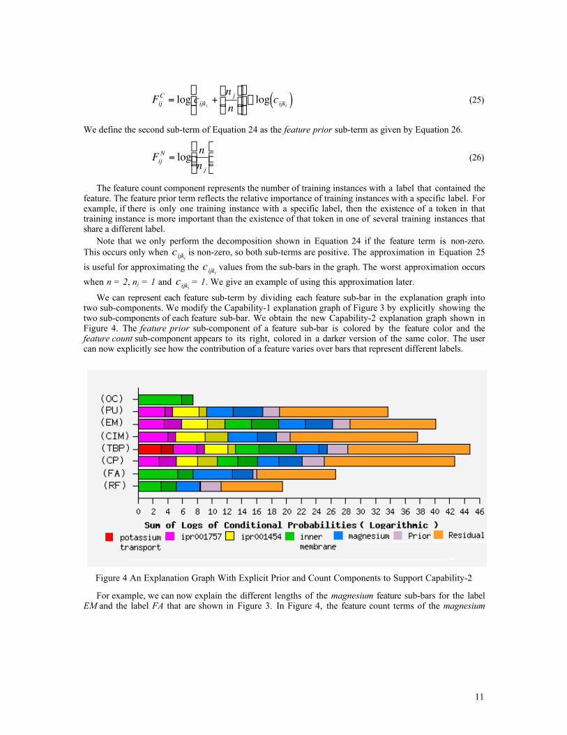
We can represent each feature sub-term by dividing each feature sub-bar in the explanation graph intotwo sub-components. We modify the Capability-1 explanation graph of Figure 3 by explicitly showing thetwo sub-components of each feature sub-bar. We obtain the new Capability-2 explanation graph shown inFigure 4. The feature prior sub-component of a feature sub-bar is colored by the feature color and thefeature count sub-component appears to its right, colored in a darker version of the same color. The usercan now explicitly see how the contribution of a feature varies over bars that represent different labels.

Figure 4 An Explanation Graph With Explicit Prior and Count Components to Support Capability-2

For example, we can now explain the different lengths of the magnesium feature sub-bars for the labelEM and the label FA that are shown in Figure 3. In Figure 4, the feature count terms of the magnesium

12

feature are represented by darker sub-bars whose length is 2.8 for the label FA and 3.7 for the label RF. Wecan use these sub-bar lengths and Equation 25 to approximate the number of labeled training instances thatcontain this feature, as computed in Equation 27.

†

F mag( ) FA( )C ª log c mag( ) FA( )1( ) ª 2.8 fi c mag( ) FA( )1 ª 7

F mag( ) EM( )C ª log c mag( ) EM( )1( ) ª 3.7 fi c mag( ) EM( )1 ª13

(27)

Although Equation 27 shows that the magnesium feature count sub-term is larger for label EM than forlabel FA, the total contribution due to the magnesium feature is the opposite for these two labels. Thedifference is isolated to the feature prior sub-terms defined in Equation 26, as shown in Equation 28.

†

F mag( ) FA( )N = log n

n FA( )

Ê

Ë Á Á

ˆ

¯ ˜ ˜ ª 5.4 fi

nn FA( )

ª 42.2

F mag( ) EM( )N = log n

n EM( )

Ê

Ë Á Á

ˆ

¯ ˜ ˜ ª 3.5 fi

nn EM( )

ª11.3

(28)

The ratio of the values 11.3/42.2 = 0.27 is the ratio of the number of training sequences (nEM) to (nFA).In other words, the feature prior sub-bar for the label FA is longer than the sub-bar for the label EM,because the number of training sequences with the label EM is only about 27% of the number of traininginstances with the label FA. Therefore, the existence of a token in one of the training instances with thelabel EM is more significant. Although we looked at the feature prior term for the feature magnesium,Equation 26 – Equation 28 are independent of features (Fi). Therefore, all non-zero feature prior terms arethe same for a fixed label (Lj).

The decomposition of a feature sub-bar, into feature prior and feature count sub-components, allows theuser to easily see the effects of both the different number of total training sequences with each label and thedifferent number of training sequences with each label that have a specific feature. The existence of even asingle training instance with a specific label that contains a token contributes the feature prior (lightcolored) contribution to the graph. In many applications, this contribution is larger than the (dark colored)contribution of all subsequent training instances with that label that contain the same feature. For example,in Figure 4, there are 24 non-zero feature sub-bars. Of these 24, only 5 cases have larger feature count sub-components (dark colored sub-bars) than feature prior sub-components (light colored sub-bars)

In summary, Capability-2 allows us to directly compare the lengths of display objects (sub-barcomponents) to determine the relationship between feature counts,

†

cijki in training instances with different

labels, and to determine the prior probabilities from the lengths.

5. Selecting Focus FeaturesA user may have a preconceived notion that the contributions of a particular feature to a classificationdecision are very important. If this feature is not included in the default focus feature set, it may benecessary to change the focus feature set to convince the user, either that the feature provides positiveevidence for the classifier’s prediction or that, even though the feature provides negative evidence, thepositive evidence contributed by other features more than compensates for the negative evidence providedby this particular feature. Therefore, an explanation facility requires a mechanism to change the focusfeature set by replacing any features in the focus feature set by any other non-focus features.

Sometimes, the user does not have a particular non-focus feature in mind, but would like to look at thecontributions of those non-focus features that have the largest chance of affecting the classification.Therefore, the mechanism that changes the focus feature set should not only support the ability to replaceany focus feature by any non-focus feature, but should also provide some kind of ranking that indicates

13

which non-focus features have the largest chance of affecting a classification. This mechanism will allow auser to gain confidence in the classification, by exploring the most important features.

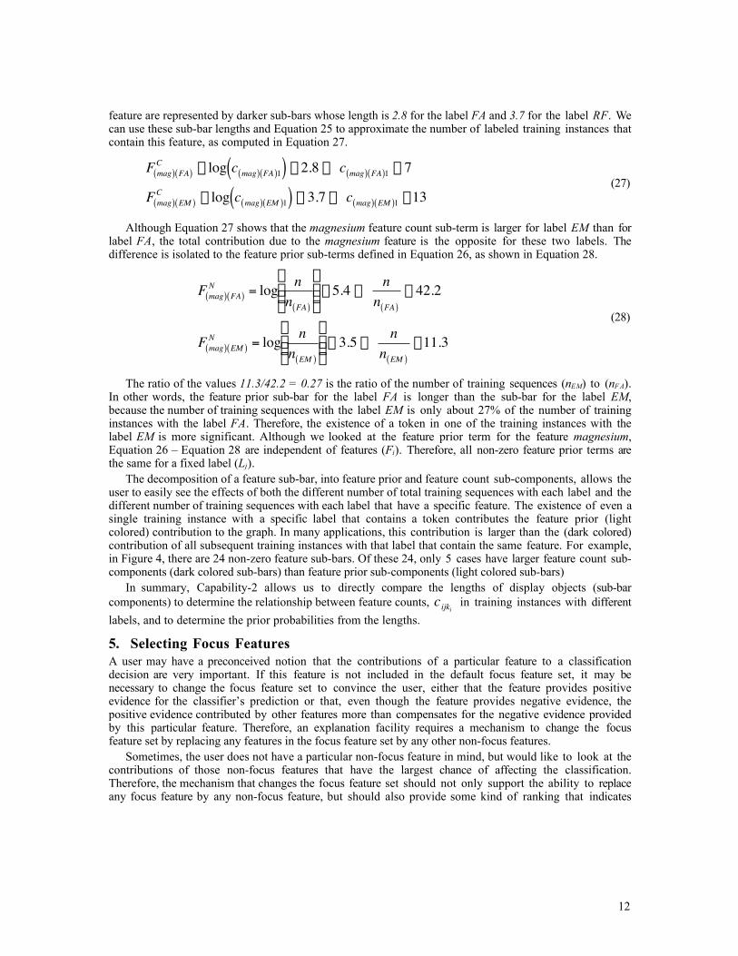
The information content (or information gain) of a feature is a measure of the amount it contributes toclassifications in general (Cover & Thomas 1991). Figure 5 shows a mechanism for replacing focus-features by non-focus features that highlights features with high information content. Features in the top95th, 85th, 70th and 50th percentiles are highlighted in different shades. The figure is clipped so that most ofthe features are not shown. The check-marks denote the 5 current focus features.

Figure 5 Selecting focus features

Since three of the non-focus features, atp-binding, hydrolase and transmembrane are in the top 95th

percentile of information content, they have the highest probability of affecting classification results overthe entire range of potential query instances. However, none of the current focus features are in this top 95th

percentile. This is not a contradiction, since no particular query instance is representative of the entire rangeof potential query instances. This example shows that for any particular query instance, it is better to selectfocus features based on feature gain, rather than information content, since they have the greatest impact onthe classification of that particular query instance.

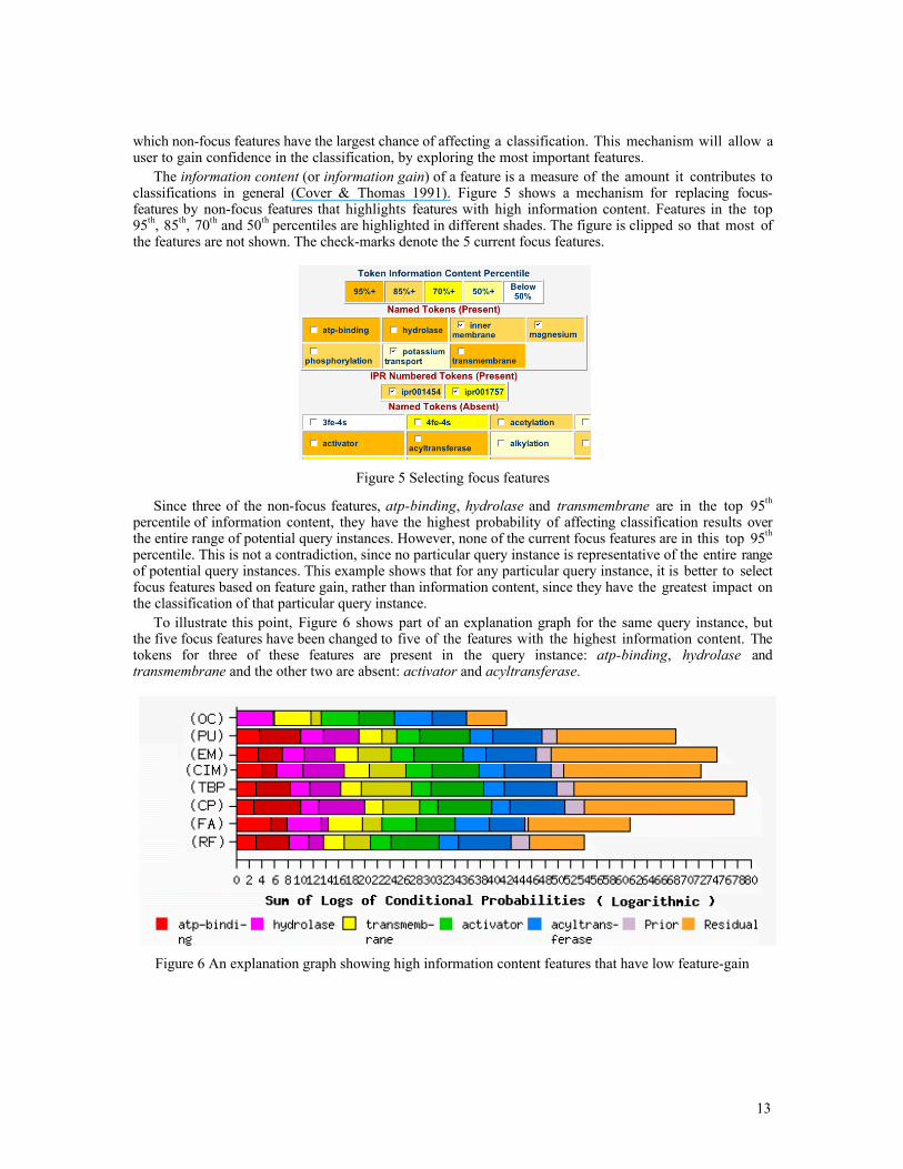
To illustrate this point, Figure 6 shows part of an explanation graph for the same query instance, butthe five focus features have been changed to five of the features with the highest information content. Thetokens for three of these features are present in the query instance: atp-binding, hydrolase andtransmembrane and the other two are absent: activator and acyltransferase.

Figure 6 An explanation graph showing high information content features that have low feature-gain

14

The total gain does not change between the favorite label TBP and any other label. However, thequality of the explanation for the difference has been degraded. First, notice that the feature gain of the twoabsent tokens (activator and acyltransferase) in the favorite label relative to all other labels is almost zero(the feature sub-bars for these two features are the same size in all bars). This is an illustration of the lackof utility of absent features in this class of applications.

Second, notice that the feature gain of the features atp-binding and hydrolase are negative for thefavorite label (TBP) relative to the contender label (CP). If the user’s intuition was highly influenced bythese two features, it would be very important to view these features so that the user can see that althoughthese two features favor the label CP, they do not favor it enough to compensate for the other features liketransmembrane (the other new focus feature), and the previous focus features: inner membrane, ipr001454,ipr001757, and potassium transport (the previous focus features), which all favor the label TBP. Given thefocus features of Figure 6, the important features are buried in the residual bar, which is now much longerfor label TBP than label CP.

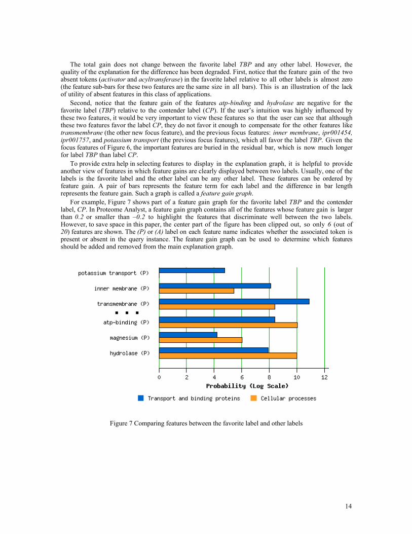
To provide extra help in selecting features to display in the explanation graph, it is helpful to provideanother view of features in which feature gains are clearly displayed between two labels. Usually, one of thelabels is the favorite label and the other label can be any other label. These features can be ordered byfeature gain. A pair of bars represents the feature term for each label and the difference in bar lengthrepresents the feature gain. Such a graph is called a feature gain graph.

For example, Figure 7 shows part of a feature gain graph for the favorite label TBP and the contenderlabel, CP. In Proteome Analyst, a feature gain graph contains all of the features whose feature gain is largerthan 0.2 or smaller than –0.2 to highlight the features that discriminate well between the two labels.However, to save space in this paper, the center part of the figure has been clipped out, so only 6 (out of20) features are shown. The (P) or (A) label on each feature name indicates whether the associated token ispresent or absent in the query instance. The feature gain graph can be used to determine which featuresshould be added and removed from the main explanation graph.

Figure 7 Comparing features between the favorite label and other labels

15

6. Capability-3: Feature ContextWhat is the source of the basic evidence and how does that evidence relate to the specific training set usedto build the classifier? Sometimes, the user may have strong (counter) intuition about contributions of afeature to the prediction probabilities of the labels provided by the classifier, as described in Section 5. Inthis case, it is useful to allow the user to inspect all of the training data related to that feature. In general,this means all of the training instances, since the absence or presence of a token in a training set can beequally important. However, for the class of applications where presence dominates absence (like PA), it isuseful to display all training instances that contain a token, sorted by the instance labels. In general, thisallows the user to see the feature in the context of other features that were present or absent and this mayhelp to convince the user of the correctness of the evidence. In some applications, the feature values may bederived from more basic data. If this is the case, the user should also be able to go back to the basic datathat was used to derive the feature values for each training instance; see Section 7.

The NB assumption states that the value of a feature in a training instance is independent of the otherfeature values. However, in practice, the user often wants to check the context. In some applications, thecontext can be even wider than the other feature values. In these cases, an explanation mechanism shouldprovide a trace of the computation of feature values from raw training instances, to allow the user toinvestigate the relationship between the raw training data, the feature values and the predicted labels. Thetrace part of this capability is very application-dependent. The user can either be convinced by seeing thetraining data, or become suspicious of the training data itself. In either case, the explanation facility hasaccomplished its goal of providing transparency.

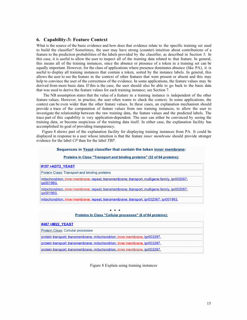
Figure 8 shows part of the explanation facility for displaying training instances from PA. It could bedisplayed in response to a user whose intuition is that the feature inner membrane should provide strongerevidence for the label CP than for the label TBP.

Figure 8 Explain using training instances

16

First, there were 32 training instances with the token inner membrane that were labeled TBP comparedto only 6 that were labeled CP. The web page actually shows all training instances that included the featureinner membrane (sorted by label) but we clipped the figure.

Second, the training instances are listed and can be examined in the context of the other features in thattraining instance. For example, of the 6 training instances labeled CP, 5 also contain the token proteintransport. On the other hand, only 1 of the 32 training instances labeled TBP also contained the tokenprotein transport.

7. Capability-4: Data TraceWhat are the application-specific computational techniques that were used to transform basic data tofeatures? In some applications, the feature values may be derived from more basic data. In this case, theuser should be able to view the basic data that was used to derive the feature values for each traininginstance. The explanation facility should provide a trace of the computation of feature values from rawtraining instances, to allow the user to investigate the relationship between the raw training data, the featurevalues and the predicted labels. The trace part of this capability is very application-dependent.

For example, in the PA application, each training and query instance is a DNA or protein sequence(string of letters). A similarity search is done against a sequence database to find the three best matches,called sequence homologs. A set of features is extracted from the database entries of each homolog of thequery sequence and the union of these three sets of features forms the feature set of the training or queryinstance, as shown in Figure 8. Each feature set is independent evidence of the impact of the feature on atraining instance. In addition, there is raw data available in this application. Each feature set is a web linkthat connects to the genetic sequence homolog of the query instance and contains a vast amount ofinformation about the homolog that a user can use to establish confidence in the computed feature set.

It is not always possible to convince a user that a classification prediction is accurate, even with thisextra data. However, it is not always desirable to convince the user that the classification is correct.Sometimes, the outcome of using an explanation facility is that the user identifies suspicious labeling oftraining data. For example, while using the PA explanation facility to explain the classification of anE.coli sequence, one of our colleagues discovered that three of the Yeast training instances were incorrectlylabeled.

8. ConclusionWe have provided a framework for explanation systems, in the context of NB classifiers (for proteinfunction prediction), and in particular, articulated 5 different capabilities that can answer five importantquestions. In doing this research, we discovered the following five points:

1) The relative contributions of individual features can be displayed in an intuitive manner byusing an additive graphical mechanism, based on logarithms (Capability-1).

2) To explain the classification of a particular instance, our approach zooms in to show thecontributions of a few focus features. These features should be selected on a per-query basis, tomaximize discrimination of the feature between the favorite label and other labels, instead ofbeing based on high information content.

3) Since a user may think that non-focus features are important in a particular classification, weprovide a mechanism to change focus features and to help the user select focus featurecandidates.

4) The contribution of a feature in a label bar depends not only on training instance counts thatexhibited the feature, but also on the relative sizes of the training sets with each label. To fullyunderstand the relative contributions of a feature to different labels, it is necessary todecompose a feature into two components (Capability-2).

5) To convince some users, it is helpful to show the context of features in the original trainingdata (Capability-3) and an application-dependent trace from raw data to features (Capability-4).Sometimes this can help identify suspicious training instances

17

Admittedly, there is more work to be done towards sound, simple and intuitive classifier explanations.However, this work lays the analytical foundation for explaining Naïve Bayes classifications. It presents aprototype system that uses bar graphs and an interactive user interface to present complex explanations in asimplified manner. As future work, we think that an explanation mechanism would benefit from a what-ifcapability. As one example, the user may feel that the query instance should have an extra token present orthat one of the present tokens should be absent. It should be possible for the user to ask how the additionor removal of a token from the query instance would affect the classification, by viewing explanationgraphs that take these hypothetical changes into account. As a second example, the user should be able toask how the classification would be different if some of the training instances were removed, or if somespecific new training instances were added, or if some training instances had their token sets changed in aparticular way. The explanation technique would also be enhanced if it could explain why some resultswere not returned.

While this paper has focused on a specific representation (Naïve Bayes) for a specific application(Proteome Analyst), the basic ideas presented are much more general. In particular, the first 3 capabilities(0-2) are completely representation, domain and application independent. For example, Capability-2 can beused whenever we can go from data samples to sufficient statistics (Ripley 1996) (such as cijk) to classifier;as such, there are definite analogues in general belief networks (Pearl 1988), and may well be analoguesrelated to decision trees (Mitchell 1997), SVMs and other species of classifiers.

AcknowledgementsThis general explanation mechanism grew out of a need to provide an explanation facility for the

Proteome Analyst project, which could be used by molecular biologists. We would like to thank CynthiaLuk, Samer Nassar and Kevin McKee for their contributions to the original prototype of Proteome Analystduring the summer of 2001. We would like to thank molecular biologists, Warren Gallin and Kathy Magorfor their valuable feedback about Proteome Analyst. We would also like to thank Keven Jewell and DavidWoloschuk from the Alberta Ingenuity Centre for Machine Learning for many useful discussions indeveloping the explanation technique. This research was partially funded by research or equipment grantsfrom the Protein Engineering Network of Centres of Excellence (PENCE), the National Science andEngineering Research Council (NSERC), Sun Microsystems and the Alberta Ingenuity Centre for MachineLearning (AICML).

ReferencesCover, T. & Thomas, J. (1991). Elements of Information Theory, New York, Wiley.Duda, R. O. & Hart, P.E. (1973). Pattern Classification and Scene Analysis, New York, Wiley.Heckerman , D.E. (1998). A Tutorial on Learning with Bayesian Networks. In Learning in Graphical

Models, Boston, MIT Press.Lacave, C., & Diez, F. J. (2000). A Review of Explanation Methods for Bayesian Networks, Tech. rep.

IA-2000-01, UNAD, Department Inteligencia Artificial, Madrid.Lidstone, G. (1920). Note on the general case of the Bayes-Laplace formula for inductive or a posteriori

probabilities. Trans. on the Fac. of Act., 8, 182-192.Mackinlay, J. D. (1986). Automatic Design of Graphical Presentations, Tech. rep. STAN-CS-86-1138,

Stanford University, Computer Science Department, Palo Alto.Myllymäki, P., Silander, T., Tirri, H. & Uronen, H. (2002). B-Course: A Web-Based Tool for Bayesian

and Causal Data Analysis. Int. J. on Artificial Intelligence Tools, 11(3), 369-387. (http://b-course.cs.helsinki.fi/)

Mitchell, T. M. (1997). Machine Learning, New York, McGraw-Hill.Pearl, J. (1988). Probabilistic Reasoning in Intelligent Systems: Networks of Plausible Inference, San

Mateo, Morgan Kaufmann.Ripley, B. (1996). Pattern Recognition and Neural Networks, Cambridge, Cambridge University Press.

18

Ristad, E. S. (1995). A Natural Law of Succession , Tech. rep. 495-95, Princeton University, ComputerScience Department, Princeton.

Teach, R. L., & Shortliffe, E. H. (1984). An analysis of physician's attitudes. In Rule-Based ExpertSystems, Reading, Addison-Wesley.

Szafron, D., Lu, P., Greiner, R., Wishart, D., Lu, Z., Poulin, B., Eisner, R., Anvik, J., Macdonell, C. &Habibi-Nazhad, B. (2003). Proteome Analyst – Transparent High-throughput Protein Annotation:Function, Localization and Custom Predictors, Tech. rep. 03-05, University of Alberta, Department ofComputing Science, Edmonton (http://www.cs.ualberta.ca/~bioinfo/PA/).