Explaining changes and trends in the airline industry: Economies of density, multiproduct scale, and spatial scope

Transportation Research Part E 60 (2013) 13–26

Contents lists available at ScienceDirect

Transportation Research Part E

journal homepage: www.elsevier .com/locate / t re

Explaining changes and trends in the airline industry:Economies of density, multiproduct scale, and spatial scope

1366-5545/$ - see front matter � 2013 Elsevier Ltd. All rights reserved.http://dx.doi.org/10.1016/j.tre.2013.09.003

⇑ Corresponding author. Tel.: +56 2 29784380; fax: +56 2 26894206.E-mail addresses: [email protected] (S.R. Jara-Díaz), [email protected] (C.E. Cortés), [email protected] (G.A. Morales).

Sergio R. Jara-Díaz ⇑, Cristián E. Cortés, Gabriela A. MoralesCivil Engineering Department, Universidad de Chile, Casilla 228-3, Santiago, Chile

a r t i c l e i n f o a b s t r a c t

Article history:Received 17 December 2012Received in revised form 12 July 2013Accepted 14 September 2013

Keywords:Air transportNetwork size and shapeRoute structureScale economiesSpatial scope

Changes in the shape and size of airline networks have not been explained clearly from acost perspective based on the finding of increasing returns to density for given route struc-tures and constant returns to scale for variable network size. We reassessed the estimatesof these economies by using new scale and scope indices, finding savings due to changes inroute structures and various types of economies of spatial scope not previously calculated:network size, trunk-local services and domestic-international services. Results contributenew insights on the role of cost incentives in the observed changes and trends in the airlineindustry.

� 2013 Elsevier Ltd. All rights reserved.

1. Introduction

Most of the empirical discussions on the organization of the airline industry have been conducted with the help of empir-ical estimations of cost functions, from which economies of density (RTD) and economies of scale (RTS) can be obtained. RTDaddresses output growth with a constant network size and route structure, whereas RTS considers changes in the networksize. Using these concepts, potential cost savings arising from output and/or network growth have been studied in the spe-cialized literature, where most authors have found increasing RTD and nearly constant RTS. According to the definitions ofboth indices, previous studies have concluded that there are cost advantages arising from increasing the flow while holdingthe network size constant (density of traffic is increased) and that there are no cost advantages for firms in operating largernetworks. However, the behavior observed in the industry has not followed these trends. After deregulation (in the US firstand then in the rest of the world), the concentration and network size of the industry have increased through mergers, acqui-sitions, and alliances. Mergers are often viewed as a way to facilitate marketing management by the airlines to build anti-competitive monopoly power in pricing. Although the search for higher profits commanded by demand has likely had a rolein this evolution, cost studies have attempted to explain network growth along with the emergence of hub-and-spoke oper-ating structures through RTD and RTS.

On the pure cost side, some authors have argued that the observed behavior of airlines can be understood ‘‘as an attemptto exploit economies of traffic density’’ (Brueckner and Spiller, 1994) and that this behavior occurs ‘‘in spite of constant re-turns to scale/network size’’ because ‘‘the addition of a station to a hub and spoke system can result in economies’’ (Oum andTretheway, 1990), which might occur because the density over the existing spokes could increase. As stated by Basso andJara-Díaz (2005), ‘‘although in principle the argument seems reasonable, the increasing returns to density found in manystudies were calculated explicitly keeping the size of the network fixed. This means that economies of density can be usedwithout ambiguity to explain the merging of firms that serve the same set of nodes but, as found in every econometric study

14 S.R. Jara-Díaz et al. / Transportation Research Part E 60 (2013) 13–26

that has considered a network variable, expanding the network is costly and this is not considered in the density justificationfor network growth’’. As shown by Kumbhakar (1990) and Liu and Lynk (1999), economies of density were important beforederegulation but are less important in the post-deregulation period. This observation has been reinforced by Swan (2002),who concluded that the main source of economies of density, namely, aircraft size, has not played as relevant a role as thechange in the route structure in recent decades. This conclusion coincides with the findings of Wei and Hansen (2003)regarding the importance of frequency over aircraft size to accommodate larger flows. Other authors have argued that analternative explanation for merging or the formation of alliances has been economies of spatial scope (see, for example, Hur-dle et al., 1989; Oum et al., 2000). The levels of efficiency that can be achieved in procurement and sharing facilities withlarger airlines have often been viewed as important. However, costs may rise as unions have more concentrated power witha single carrier, and wage rates may shift toward the higher level of the two merging companies.

Thus, the changes observed in the airline industry have been interpreted and explained using estimated cost functions indifferent ways, generating interesting discussions and debate. In this paper, we first review the empirical literature in airtransport from 1984 to 2012, synthesizing the analysis and conclusions regarding industry structure based on estimationsof RTD and RTS. We then present three new indices that have been developed in the literature to replace the prevailing scalemeasures: RTD0, the corrected version of RTD, which examines costs as flows expand holding the route structure constant;the multioutput degree of scale economies (S), which considers costs as flows expand allowing for the readjustment of theroute structure; and economies of spatial scope (SC), which examines the advantages or disadvantages of serving two dis-tinct sets of flows. We find that RTD < RTD0 < S and that there are various types of economies of spatial scope, including net-work size, trunk-local services, and domestic-international services. These results advance beyond previous analyses of therole of cost incentives behind the observed changes and trends in the airline industry. Route forms and network shapes andsizes could also be driven by demand characteristics, although these effects are not analyzed here. Strategic interactionamong competitors also contributes to the structure of air networks (Oum et al., 1995).

In the next section, the concepts of RTD and RTS are presented, and their application to the analysis of the air industry issummarized. The new indices developed in the transport economics literature are then introduced and justified. The use ofthese new indices to re-examine each case is presented in Section 3. Finally, a synthesis and conclusions are offered inSection 4.

2. Cost functions in air transport

2.1. Empirical estimates of returns to density and returns to scale: a synthesis

The multioutput degree of economies of scale, S, is defined by the maximal proportional expansion of output Y that isfeasible after a proportional expansion of inputs X, such that a value of S larger than, equal to, or smaller than one impliesincreasing, constant, or decreasing returns to scale, respectively (Panzar and Willig, 1977). Although S is defined based on thetechnology, S can be calculated from the cost function C(w, Y), which represents the minimum expenditure necessary to pro-duce Y at input prices w, as

S ¼ CðYÞPiyi

@C@yi

¼ 1Pigi; ð1Þ

where gi is the elasticity of C with respect to the ith output. Input prices are omitted for notational simplicity. Note that S > 1implies that a proportional expansion of Y induces an increase in cost by a smaller proportion.

The large size that the output vector Y achieves in the transport sector (i.e., flows in very many origin–destination (OD)pairs) precludes its direct use in the empirical work, as noted by various authors. Thus, cost functions must be estimatedusing aggregate output descriptions, eY ¼ f~yhg, such as ton-kilometers or seat-kilometers, and so-called attributes, such asaverage distance or load factor. When a network size variable N is used, empirical studies of transport industries distinguishbetween two concepts of ‘scale’: returns to density (RTD) and returns to scale (RTS), as first proposed by Caves et al. (1984). Inthe former case, the network is assumed to be fixed as output increases, i.e. traffic density increases. In the latter case, bothoutput and network size increase, with traffic density remaining unchanged. RTD is calculated as the inverse of the sum of asubset of the cost-output elasticities (this subset varies from study to study and has thus become a source of ambiguity). InRTS, the elasticity of the network size is also included in the calculation. Note that RTD represents an attempt at capturingwhat S actually measures, i.e. the change in cost as output expands. RTS was designed to address the cost effects of networkexpansion, i.e., a variation in N.

In the airline market literature, most authors estimate a cost function considering similar outputs and attributes in thespecification. In Table 1, we summarize the literature covering 30 years during and after deregulation of US, Canadian,and European markets. Output and the so-called attributes are assumed to be exogenous in these studies. Overall, a translogform has been used to specify the cost function and, in all cases, the number of points served, PS, is used as the indicator ofnetwork size N. The typical output aggregates are of the form flow � distance, such as revenue passenger mile (RPM) andrevenue ton miles (RTM), as discussed in Oum and Zhang (1991), Liu and Lynk (1999), and Creel and Farell (2001). In somecases, the aggregates are grouped into one variable called multilateral output index (Caves et al., 1984; Kumbhakar, 1990;Windle, 1991; Oum and Yu, 1998). The hedonic output (grouping each aggregate with its associated attributes) introduced

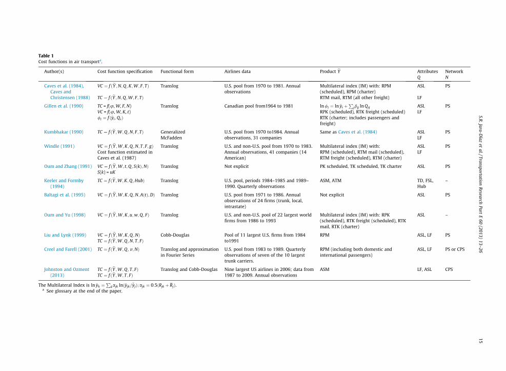
Table 1Cost functions in air transporta.

Author(s) Cost function specification Functional form Airlines data Product eY AttributesQ

NetworkN

Caves et al. (1984),Caves andChristensen (1988)

VC ¼ f ðeY ;N;Q ;K;W ; F; TÞ Translog U.S. pool from 1970 to 1981. Annualobservations

Multilateral index (IM) with: RPM(scheduled), RPM (charter)

ASL PS

TC ¼ f ðeY ;N;Q ;W; F; TÞ RTM mail, RTM (all other freight) LF

Gillen et al. (1990) TC = f(u, W, F, N) Translog Canadian pool from1964 to 1981 ln /i ¼ ln ~yi þP

jbij ln Qij ASL PSVC = f(u, W, K, t) RPK (scheduled), RTK freight (scheduled) LF/i ¼ f ð~yi;QiÞ RTK (charter; includes passengers and

freight)

Kumbhakar (1990) TC ¼ f ðeY ;W;Q ;N; F; TÞ Generalized U.S. pool from 1970 to1984. Annualobservations, 31 companies

Same as Caves et al. (1984) ASL PSMcFadden LF

Windle (1991) VC ¼ f ðeY ;W;K;Q ;N; T; F; gÞ Translog U.S. and non-U.S. pool from 1970 to 1983.Annual observations, 41 companies (14American)

Multilateral index (IM) with: ASL PSCost function estimated inCaves et al. (1987)

RPM (scheduled), RTM mail (scheduled),RTM freight (scheduled), RTM (charter)

LF

Oum and Zhang (1991) VC ¼ f ðeY ;W; t;Q ; SðkÞ;NÞS(k) = uK

Translog Not explicit PK scheduled, TK scheduled, TK charter ASL PS

Keeler and Formby(1994)

TC ¼ f ðeY ;W;K;Q ;HubÞ Translog U.S. pool, periods 1984–1985 and 1989–1990. Quarterly observations

ASM, ATM TD, FSL,Hub

–

Baltagi et al. (1995) VC ¼ f ðeY ;W;K;Q ;N;AðtÞ;DÞ Translog U.S. pool from 1971 to 1986. Annualobservations of 24 firms (trunk, local,intrastate)

Not explicit ASL PS

Oum and Yu (1998) VC ¼ f ðeY ;W;K;u;w;Q ; FÞ Translog U.S. and non-U.S. pool of 22 largest worldfirms from 1986 to 1993

Multilateral index (IM) with: RPK(scheduled), RTK freight (scheduled), RTKmail, RTK (charter)

ASL –

Liu and Lynk (1999) VC ¼ f ðeY ;W;K;Q ;NÞ Cobb-Douglas Pool of 11 largest U.S. firms from 1984to1991

RPM ASL, LF PSTC ¼ f ðeY ;W;Q ;N; T; FÞ

Creel and Farell (2001) TC ¼ f ðeY ;W;Q ;v ;NÞ Translog and approximationin Fourier Series

U.S. pool from 1983 to 1989. Quarterlyobservations of seven of the 10 largesttrunk carriers.

RPM (including both domestic andinternational passengers)

ASL, LF PS or CPS

Johnston and Ozment(2013)

TC ¼ f ðeY ;W;Q ; T; FÞ Translog and Cobb-Douglas Nine largest US airlines in 2006; data from1987 to 2009. Annual observations

ASM LF, ASL CPSTC ¼ f ðeY ;W; T; FÞ

The Multilateral Index is ln ~yk ¼P

kajk lnð~yjk=�~yjÞ;ajk ¼ 0:5ðRjk þ RjÞ.

a See glossary at the end of the paper.

S.R.Jara-D

íazet

al./TransportationR

esearchPart

E60

(2013)13–

2615

16 S.R. Jara-Díaz et al. / Transportation Research Part E 60 (2013) 13–26

by Spady and Friedlaender (1978) has been used only by Gillen et al. (1990). Regarding attributes, the authors typically usethe load factor (LF), representing use of the available capacity, and the average stage length (ASL) as a measure of the networkarcs served by an airline. Based on these aggregates and attributes, policy conclusions were deduced from the calculation ofRTD and RTS obtaining increasing returns to density (RTD > 1) and constant returns to scale (RTS ffi1). The studies also con-sider variables accounting for technical change, including t, T, F, and A(t) as defined in the glossary; these variables control foreffects over time such that RTD and RTS capture the role of outputs and attributes only.

While these studies were being conducted and reported, the scale indices used began to be re-examined from differentangles (Gagné, 1990; Ying, 1992; Xu et al., 1994; Jara-Díaz and Cortés, 1996; Oum and Zhang, 2000). Today, we can interpretthis process based on a general observation: the output measures were largely interrelated, which made the output elastic-ities interdependent. According to Jara-Díaz and Cortés (1996), the connection between the different output measures wasthe underlying vector of flows produced by a transport firm.

2.2. A framework for reassessing the scale and scope indices

Omitting the dimensions ‘‘cargo type’’ and ‘‘period’’ for simplicity, the output of a transport firm is a vector Y of flows yij

between many OD pairs (Jara-Díaz, 1982a,b; Winston, 1985; Ying, 1992; Braeutigam, 1999). Following Jara-Díaz (2007), for agiven OD structure of flows (defined by vector Y), the technical challenge for a transport firm is to decide on the number andcapacity of vehicles, design of ways and terminals, and frequencies, among other considerations. As transport occurs on anetwork, the firm must also choose a service structure (the generic way in which vehicles visit the nodes) and a link se-quence, which are endogenous decisions that define a route structure. The service structure can take the form of a seriesof point-to-point services, a cyclical system, or a hub-and-spoke system, among other options. The route structure is simplythe actual paths that the vehicles follow on a given network within a service structure. Thus, S considers all of these decisionswhen the output expands proportionally on a given physical network (Jara-Díaz and Basso, 2003), which appears to be cap-tured by RTD. Serving new OD pairs means an expansion of the production line, which might induce an expansion of thefirm’s network. This expansion requires one to examine whether it is more cost convenient for a firm to expand its networkto serve new flows or for another firm to serve these new OD pairs. The idea behind RTS is precisely to capture this decisionthrough the impact of a variation in PS. However, there is a specific cost measure that has been developed to analyze outputpartitions: economies of scope.

Let D be the set of all outputs and A and B be an orthogonal partition of D (i.e., A[B = D and A\B = £). Then, the degree ofeconomies of scope is defined as

SCA ¼ SCB ¼CðYAÞ þ CðYBÞ � CðYDÞ

CðYDÞ; ð2Þ

where YA is vector YD with yi = 0, " i R A � D and YB is defined analogously. A negative value for SCA indicates that it is lessexpensive to have a second firm producing YB rather than to expand the production line of a firm already producing YA. If SCA

is positive (economies of scope), it is less expensive for a single firm to produce YD. It is easy to verify that �1 < SC < 1. As Y isa vector of OD flows, the question that RTS attempts to answer through the aggregates is adequately considered when ana-lyzing economies of spatial scope.

Thus, S and SC in transport activities in general and in air transport in particular are unambiguously defined after iden-tifying output, inputs, and technology: S examines the behavior of costs as flows expand proportionally, whereas SC ad-dresses cost changes after the addition of new flows. Both indices help to investigate potential changes in all of theelements mentioned above, including the number and capacity of vehicles, design of ways and terminals, frequencies, routestructures, and network size. Do RTD and RTS perform the same job?

Behind the aggregates included in the vector eY ¼ f~yhg used to estimate air cost functions and to calculate RTD and RTS liesthe real output Y of an airline, i.e., ~yh ¼ ~yhðYÞ. If the estimated function eCðeY ; PSÞ is taken as a good approximation using aggre-gates of the cost function of the firms, then the characteristics of the multi-output cost function should be obtainable fromthe estimated parameters of eCðeY ; PSÞ by noting that eCðeY ; PSÞ ¼ eCðeY ðYÞ; PSÞBeCðYÞ, considered an implicit representation ofthe (true) cost function in terms of Y. Using this approach, Jara-Díaz and Cortés (1996) found that an estimator bS of S canbe calculated as

bS ¼ Xi

gi

" #�1

¼X

j

aj ~gj

" #�1

; aj ¼X

i

eji ð3Þ

where eji is the elasticity of aggregate output ~yj with respect to yi and ~gj is the elasticity of eC with respect to ~yj. The values foreji are obtained from ~yhB~yhðYÞ , and the values for ~gj are estimated from eCðeY ; PSÞ. Thus, the calculation of bS is both rigorousand feasible, as the calculation respects the original definition of S in Eq. (1) while using the estimated cost function eCðeY ; PSÞ.Note that aj is the degree of homogeneity of the jth aggregate with respect to the disaggregated flows, and its calculationavoids the ambiguity previously mentioned regarding which aggregate should be considered in the calculation of S.

As the elasticity of PS is not included in Eq. (3), this method can be viewed as an improved version of RTD, as argued byOum and Zhang (2000). However, this fact does not mean that the corrected RTD (henceforth called RTD0) is actually S, as

S.R. Jara-Díaz et al. / Transportation Research Part E 60 (2013) 13–26 17

suggested by Panzar (1989), because RTD assumes that the route structure also remains unchanged, as noted by Basso andJara-Díaz (2006a), a condition that is also included in RTD0. This condition is required because the idea of estimating RTD is toanalyze whether ‘‘the average costs of a direct connection decreases with proportionate increases in both flows on that con-nection’’ (Hendricks et al., 1995), which means that only the existing links handle the new traffic. If the route structurechanges, some new links may be added, whereas others may disappear. Along these lines, Basso and Jara-Díaz (2006a) pro-posed to use Eq. (3) to calculate both RTD0 and S but assumed that the route structure is fixed in the former and variable inthe latter. This distinction induces differences in the calculation of the aj. For example, in RTD0, the aj of the average distancewill always be zero, as flows grow by the same proportion while holding the route structure fixed. The aj of the average dis-tance could differ from zero in S if the minimum cost is reached using a different route structure once flows increase, as aver-age distance will change (very likely diminish). We consider this distinction to be useful and relevant. Economies of densitywill be useful to know if, for example, there are economies of vehicle size, i.e., if larger flows in non-stop routes implydecreasing average costs in that route due to the use of larger vehicles.1 Hub-and-spoke networks would be strongly influencedby the existence of economies of density. Economies of scale S are important because when traffic increases significantly, it maynot be efficient to increase the size of the vehicles further or to increase frequency, which may be expensive because of conges-tion at airports. However, with a reconfiguration of the route structure, the increases in flows may be handled without increas-ing costs substantially, such as through point-to-point service in certain OD pairs, a phenomenon that has been observed inreality (see Swan, 2002).2 As is evident, S represents the optimal (efficient) adjustment of all inputs and operating rules for agiven network size and is thus expected to be larger than or equal to RTD0 if the route structure is already optimal (Kraus,2008). There is no a priori theoretical relationship between RTD and RTD0 because the relationship will depend on the aj ofthe aggregated outputs and attributes used.

As explained above, RTS is aimed at analyzing the behavior of costs when both traffic and PS increase by the same pro-portion. As the proportional increase is applied simultaneously to the vector of aggregates eY ¼ f~yhg (or to a subset) and to PS(i.e., new OD pairs emerge), analytical conditions are imposed on the OD flow vector that would be indefensible in mostcases, as shown by Basso and Jara-Díaz (2006b). As stated earlier, the variation of the number of OD pairs implied by achange in PS is a variation of the dimension of Y, which should be examined with a scope analysis.3

The empirical problem is that a direct calculation of SC using Eq. (2) is not feasible because of the dimension of the trans-port output vector. However, rescuing the property eCðeY ; PSÞ ¼ eCðeY ðYÞ; PSÞBeCðYÞ suggests a way to address the problem: asmost aggregates ~yh are implicit functions of Y, the (disaggregate) output vectors YA, YB, and YD can be used to evaluate thecorresponding aggregate vectors eY ðYAÞ, eY ðYBÞ, and eY ðYDÞ to calculate SC from eCðeY ; PSÞ as suggested by Jara-Díaz et al.(2001), i.e.,

1 Airlflying u

2 Anonto ma

3 Som

SCA ¼ SCB ¼eCðeY ðYAÞ; PSAÞ þ eCðeY ðYBÞ; PSBÞ � eCðeY ðYDÞ; PSDÞeCðeY ðYDÞ; PSDÞ

ð4Þ

The problem is then reduced to the calculation of the aggregates under different orthogonal partitions of Y when possible.By definition, partitions of Y involve zero values for some flows. As aggregates (such as total passengers or ton-kilometers)

do not go to zero when only some OD flows are zero, the arguments of eCðeY ; PSÞ in Eq. (4) are likely never evaluated at zero, asis the case with some components of YA or YB in C(�) in Eq. (2). Analytically, the challenge is different from the calculationsbehind the coefficients aj for either RTD or S because many orthogonal partitions can be analyzed. Evaluating the aggregatesrequires a careful choice of procedures on a case-by-case basis. Let us provide a simple example.

Consider an aggregate such as ton-kilometers TK. In this case, if dij denotes the distance to travel from origin i to desti-nation j, the function ~yhB~yhðYÞ would be given by

TK ¼X

ij

yijdij � TKðYÞ ð5Þ

For simplicity, assume that the route structure does not change after a variation in the OD flows. Then, the value of aTK isunambiguously equal to one following procedure (3), as shown by Jara-Díaz and Cortés (1996). The elasticity of TK shouldthen be considered to calculate bS, as in Eq. (3), with its full value. When SC is analyzed, a partition of Y should be consideredto calculate Eq. (4). Consider a partition of Y defined by YA and YB so that Y = YA + YB and YA�YB = 0. The challenge is to findTK(YA) and TK(YB), which in this simple case is

TKðYLÞ ¼Xij2TL

yijdij TL ¼ fi; j=yij 2 YLg; L ¼ A; B ð6Þ

Therefore, TK(YA) + TK(YB) = TK(Y). If TK were the only aggregate in eC , then eCðeY ; PSÞ in Eq. (4) would be the aggregate costfunction evaluated at different levels of a scalar different from zero (which might be one reason why this computationhas been viewed as a scale issue in the past; see footnote 3). If other aggregates are present, the challenge is to search for

ines have been trying to move toward 737/A320 type aircraft with lower unit costs and eliminate inefficient regional jet flying, i.e., aircraft capable ofp-to medium-haul routes, carrying no more than 100 passengers.example of the reconfiguration of a route structure is Delta at Memphis – the former Northwest hub which competed with Atlanta – as they refocusedrkets in Texas, Oklahoma, etc., where both Delta and Northwest were previously weak, while reducing duplication with Atlanta in the Southeastern US.e authors have hinted that RTS and SC are somehow related (Daughety, 1985; Hurdle et al., 1989; Borenstein, 1992).

Table 2From RTD and RTS to scale and scope.

Literature Proposed Calculations

RTD ¼P

j2J ~gj

h i�1! RTD0 ¼

Pjaj ~gj

h i�1; aj ¼

Pi@~yj

@yi

yi~yj

constant route structure

S ¼P

jcj ~gj

h i�1; cj ¼

Pi@~yj

@yi

yi~yj

variable route structure

RTS ¼P

j2J ~gj þ ~gPS

h i�1! SCR ¼ eC ðeY ðYRÞ;PSRÞþeC ðeY ðYM�RÞ;PSM�RÞ�eC ðeY ðYM Þ;PSÞeC ðeY ðYM Þ;PSÞ

18 S.R. Jara-Díaz et al. / Transportation Research Part E 60 (2013) 13–26

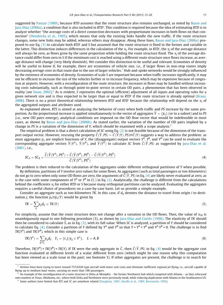
the implicit aggregation function, which will not be always as simple as Eq. (6), as shown in the next section. The choice ofaggregates is not ours; we take what the authors have used and then apply the appropriate treatment to all outputs in thenext section.

For synthesis, and emphasizing the spatial dimension of output in the transport case, with S, one analyzes the behavior ofcosts after an equiproportional expansion of the OD flows, keeping the number of OD pairs constant. In contrast, with SC, oneanalyzes the behavior of cost when new OD flows are added. To perform this analysis properly from cost functions withaggregate output, the relationship between each aggregate and the true output vector must be revealed to calculate scaleand scope consistently for policy analysis. We have shown that this procedure implies replacing the calculation of RTDand RTS by three measures: a corrected RTD (RTD0), the multioutput degree of scale economies S, and spatial SC, as summa-rized in Table 2.

3. Reassessing economies

3.1. Context of calculations

In this section, we summarize our calculations of RTD0, S, and SC for those articles in the air transport industry reported inTable 1 that contain relevant information to apply the approach described in Section 2. The intention of these calculations isto reveal the behavior of costs when output expands proportionally (all flows increase by the same proportion) and whenoutput splits into two distinct subsets of flows (orthogonal partition). The emphasis is on reassessing RTD (which yieldsRTD0), computing S, and calculating SC. As explained above, the consistent computation of the indicators requires identifyingthe relationships between the aggregates used in each case and the output vector (flows). The calculation of the correctionfactors for the (aggregate) elasticities follows the procedure presented by Jara-Díaz and Cortés (1996). However, obtainingthe values of the aggregates for various orthogonal partitions of the output vector (flows) to calculate different types of scopeis not as straightforward as in the example given in Eq. (6) for ton-kilometers; in fact, in most cases, this process can be quitecomplex, as shown in Section 3.2. The SC calculations are performed for those interesting output partitions that satisfy threefeasibility conditions: (i) the data contain observations that include the type of services analyzed (e.g., domestic-interna-tional, local-trunk); (ii) the authors provide sufficient information on cost function-related parameters (e.g., elasticities)and data used (e.g., value of the variables at the point of approximation); and (iii) information needed to complement thedescription of the partition can be collected (e.g., spatial data as cities served during the corresponding period). However,it is important to use the same treatment on each aggregate to construct the partition whenever that aggregate is usedby different authors.

3.2. Examples of the evaluation of aggregates for orthogonal partitions of output

The problem of finding the values of the aggregates for orthogonal partitions of the output vector to evaluate the elementsassociated with firms A, B, and D in Eq. (4) is very simple in some cases, e.g. ton-kilometers in Eqs. (5) and (6), and quitecomplex in other cases. Here, we first present the construction of a partition using this same type of output (flow � distance)from data with overlapping networks. Then, we develop the case of two so-called attributes that are particularly complex.Among the additional information (not reported in the original papers) that is necessary to implement the proposed SC cal-culations regarding space, we can mention the network maps of the airlines for the specific periods of study, from which thetravelled distances (linked to ASL and ALH, among others) and the points served by each company can be obtained and usedfor relevant calculations and a sensitivity analysis. This exogenous information represents actual industry changes ratherthan theoretical constructs. This spatial information is also needed for the critical first step, namely, the construction of spa-tial orthogonal partitions, which could be problematic in some cases, as firms in a cross section could present overlappingservices. In such a case, we require a pre-process to create strict orthogonal partitions of the product, as discussed below.

Let us consider two firms (A and B) with PSAB being the number of overlapping points such that PSAB(PSAB � 1) representsthe overlapping OD pairs. To find a representative value for the aggregates that would correspond to an orthogonal partitionof the disaggregate (true) flow vector, we can correct the original aggregates by subtracting the (unknown) flows served byone firm (say, B) in the shared OD pairs and adding them to the other firm. Let us illustrate this procedure for the case of

S.R. Jara-Díaz et al. / Transportation Research Part E 60 (2013) 13–26 19

aggregates typically called ‘‘product’’ in the literature, e.g., Ton, Pax, RPK, and RTK. How much aggregate flow should betransferred? Following Basso and Jara-Díaz (2005), we assume that the average flow of type j served by firm B, AODB

j (totalflow of firm B over PSB) applies to the overlapping zone as well so that the flows that have to be ‘‘transferred’’ from B to A addup to AODB

j PSABðPSAB � 1Þ. To convert this quantity into the most used aggregate product of the type ‘‘flow � distance’’, itmust be multiplied by the average length of haul ALHj. In this case, the corrected aggregates for the case of freight would be

RTKA0 ¼ RTKA þ ALHBAODBTonPSABðPSAB � 1Þ ð7Þ

RTKB0 ¼ RTKB � ALHBAODBTonPSABðPSAB � 1Þ ð8Þ

Then, RTKD ¼ RTKA þ RTKB ¼ RTKA0 þ RTKB0 would be the aggregate product for firm D in Equation (4). This calculation allowsus to properly compute economies of scope. Note that this correction is not necessary when potential savings from mergingare analyzed.

Next, we develop the detailed procedures to compute, for relevant orthogonal partitions of the true output, the values oftwo aggregates frequently used in air transport: the average stage length (ASL) and the load factor (LF). Both are labeled asattributes, but a label does not preclude their dependence on the disaggregate output vector, as discussed in Section 2.

First, let us describe the analysis for ASL. The original definition of ASL is the total length of all segments served by anyfirm, say, firm k, LTk, divided by the total number of arcs of the firm, NTk. The maximum number of segments served by afirm k, attending PSk points, is PSk(PSk � 1)/2. Therefore, NTk can be written as Nk = hkPSk(PSk � 1) with hk e (0; 1/2). ASLD

can be calculated noting that NTD = NTA + NTB and LTD = LTA + LTB, which yields

ASLD ¼ LTD

NTD ¼hAPSAðPSA � 1ÞASLA þ hBPSBðPSB � 1ÞASLB

hAPSAðPSA � 1Þ þ hBPSBðPSB � 1Þð9Þ

Let us define l = hB/hA as a non-dimensional parameter quantifying the density of the network (in terms of segments or arcs)of B with respect to A. Then, ASLD can be written as a weighted average of ASLA and ASLB associated with firms A and B, respec-tively. Analytically,

ASLD ¼ PSAðPSA � 1ÞPSAðPSA � 1Þ þ lPSBðPSB � 1Þ

ASLA þ lPSBðPSB � 1ÞPSAðPSA � 1Þ þ lPSBðPSB � 1Þ

ASLB ð10Þ

Expression (10) depends on the way in which the information about points served is reported by the authors (Eq. (10) wasused to obtain the hedonic output values as well). Finally, defining s = PSAB/PSB, the points served by firm D are given byPSD = PSA + (1 � s)PSB .

Eq. (10) for ASL cannot always be computed. The correct (feasible) computation follows a case-by-case approach and de-pends on several aspects, such as the information provided by the authors within each application, the combination of aggre-gates used, and the cost function specification, among others. Another relevant aspect is the availability of information thatcan be obtained from other sources (different from the information provided in the paper) corresponding to a similar periodof analysis and preferably for the same sample of firms. For example, in our analysis of Gillen et al. (1990), we could use Eq.(10) to compute ASL for the merged firm as a function of the number of points served (PS) and the specific ASL values of theexisting firms (reported) in combination with other sources. For our analysis of the potential cost of merging the operation oftrunk and local companies from Caves et al. (1984), the value of ASL for different PS levels was obtained by means of a linearregression, including a dummy variable to differentiate trunk from local firms. Analytically,

ASL ¼ �424:567ð�1:61Þ

þ10:19PSð2:45Þ

þ440:41dð10:72Þ

R2 ¼ 0:956 ð11Þ

where the dummy d is one if the firm is trunk and zero otherwise (Student-t values in parentheses). With this formula, cal-ibrated from the paper information together with other reasonable assumptions, several SC calculations were conducted, asdiscussed below.

Another relevant attribute used in cost functions of airlines is LF. We developed ad hoc methodologies for each studiedcase regarding LF to compute different SC indicators. For example, in the analysis of trunk-local SC in Caves et al. (1984), weassumed that the trunk and local OD pairs were served with different fleets. Therefore, the total seat-kilometers (SK) could beconsidered as additive. Under these conditions, if A, B, and D are the trunk, local, and trunk-local firms, respectively, then

SKD ¼ SKA þ SKB ð12Þ

From the definition of LF as the ratio between revenue-passenger kilometers (RPK) and seat-kilometers (SK), we obtain

LFD ¼ RPKA þ RPKB

SKD ¼ SKALFA þ SKBLFB

SKA þ SKB ¼ LFA

1þ ðSKB=SKAÞþ LFB

1þ ðSKA=SKBÞð13Þ

In Eq. (13), the ratio SKB/SKA can be written as a function of the LF values as follows

20 S.R. Jara-Díaz et al. / Transportation Research Part E 60 (2013) 13–26

SKB

SKA ¼RPKB

LFB

LFA

RPKA ¼ð1� kAÞRPMD

LFB

LFA

kARPMD ¼ð1� kAÞ

kA

LFA

LFB ð14Þ

where kA ¼ RPMA=RPMD, a ratio that can be calculated explicitly from the information reported in Caves et al. (1984). Finally,LF for the trunk-local firm can be computed as

LFD ¼ LFALFB

ð1� kAÞLFA þ kALFB ð15Þ

The same method can be adapted to cases where the factor kA cannot be computed directly. In such cases, additional assump-tions should be made to estimate the factor kA properly.

3.3. Summary of the calculations and cost implications

In Table 3, we present a summary of the application of the approach discussed covering a period of 30 years of research inthe area, including the original results for RTD and RTS and the analytical procedures for the reassessment together with thenew results. The reassessed indices are valid around the points of approximation used in the empirical cost functions esti-mated in the papers. Therefore, the analysis of results and the corresponding policy implications should be made consideringthe periods of the observations and the diversity of firms included in the authors’ data, presented in the fourth column ofTable 1. The reassessments are made without questioning either the acquisition and treatment of data or the formulationand estimation of the cost functions. Furthermore, other relevant factors, such as demand behavior or potential efficiencyproblems not analyzed by the authors, are beyond the scope of the analysis of results. These reassessments were made usingcost functions that control for changes in technology in different ways so that our RTD0, S and the scope measures below arenot biased by these effects.

All five articles that compute RTD and RTS explicitly find increasing returns to density and nearly constant or increasing(network) scale, as advanced in the introduction. From the reassessment of the indices we can visualize the existence ofincreasing returns to density (RTD0 > 1) and increasing multioutput economies of scale (S > RTD0 > 1), which shows costsincentives for the firms not only to increase network density but also to restructure schedules and routes, which is an impor-tant result. These concepts are interrelated because increasing density means larger flows on the same network, which couldbe better accommodated by changing the route structure and operational policies. Had routes and operations been optimal,we would have obtained S = RTD0 (Kraus, 2008).

The results from incremental spatial scope (i.e., adding one point served at a time as done in Basso and Jara-Díaz (2005))indicate network merging and trunk-local and domestic-international types of scope economies. The presence of these typesof economies of spatial scope indicates that there are advantages on the cost side from jointly serving markets that generatelarger networks, a conclusion that is also supported by the regional analysis of Windle (1991). The Canadian market analysisindicates that small firms needed to merge both to save costs and compete with large companies. These findings are dis-cussed in more detail below.

From our calculations of SC regarding the North American airline market, we observe the existence of positive economiesof scope of different types and for different periods, which helps in the understanding of some observed phenomena. First,from data collected before the market deregulation in 1976, we computed positive trunk-local economies of scope (refer toCaves et al., 1984), which contributes to the explanation of why firms started working under hub-and-spoke configurationsto obtain cost advantages from the coordination of terminal operations among trunk and local companies. Second, the ob-served expansion of destinations offered by the companies can be better understood from the new analysis of incrementalspatial scope economies using the data from Formby et al. (1990). Over time, the North American companies realized thatthey saved costs when expanding the spatial scope of services, a result supported by our scope calculations complementingthe returns to density already detected.

Third, regarding our finding of positive domestic-international scope economies, we conclude that in the 1980s, the firmsperceived incentives to grow by operating on larger networks. Interestingly, using the results reported by Creel and Farell(2001) based on the seven largest US firms between 1983 and 1989, we obtained SC = 0.12 for domestic-international ser-vices, which is similar to the value obtained for the largest US company using the results from Oum and Yu (1998) coveringthe 1986–1993 period. For the remaining firms (21 largest US-World), we obtained 0.066 6 SC 6 0.078, which is closer to thevalue of 0.05 obtained using the data from Liu and Lynk (1999), who analyzed the 11 largest US airlines in the 1984–1991period. These types of economies of spatial scope suggest cost-saving incentives for the observed behavior of the firms whenforming powerful alliances (such as One World Alliance) to avoid the restriction from operating in certain strategic markets.This reasoning is also supported by the observed change of other relevant firms’ attributes over time, such as ASL (see Sec-tion 3.2), with a relevant impact on costs and SC.

Regarding the Canadian airline market, our computations of SC (using the results of Gillen et al., 1990) to capture poten-tial savings from merging indicate negative values in most cases, with the exception of Nordair-EPA, where SC > 0. To inter-pret this last result, let us note that in terms of both volume and PS, before the 1980s, there was one large firm (Air Canada),several medium-sized firms (such as CPair), and several small companies (such as Nordair and EPA). We concluded thatmerging was convenient only between small firms, not only to increase their destinations but also to save costs as a resultof the joint operation in terminals. Previously, the incremental spatial scope analysis of Basso and Jara-Díaz (2005) had

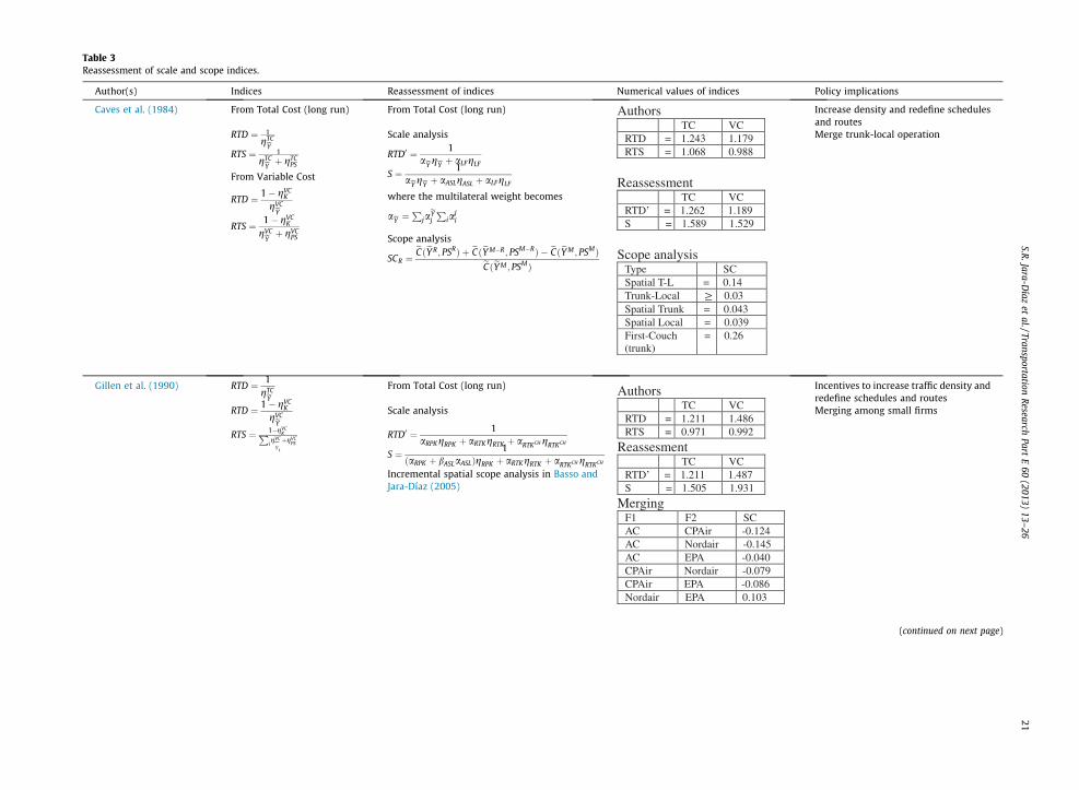
Table 3Reassessment of scale and scope indices.

Author(s) Indices Reassessment of indices Numerical values of indices Policy implications

Caves et al. (1984) From Total Cost (long run) From Total Cost (long run) Increase density and redefine schedulesand routes

RTD ¼ 1

gTCeY Scale analysis Merge trunk-local operation

RTS ¼ 1

gTCeY þ gTCPS

RTD0 ¼ 1aeY geY þ aLFgLF

From Variable Cost S ¼ 1aeY geY þ aASLgASL þ aLFgLF

RTD ¼ 1� gVCK

gVCeY where the multilateral weight becomes

RTS ¼ 1� gVCK

gVCeY þ gVCPS

aeY ¼PjaeYj Piaji

Scope analysis

SCR ¼eCðeY R; PSRÞ þ eCðeY M�R; PSM�RÞ � eCðeY M ; PSMÞeCðeY M ; PSMÞ

Gillen et al. (1990) RTD ¼ 1gTCeY From Total Cost (long run) Incentives to increase traffic density and

redefine schedules and routesRTD ¼ 1� gVC

K

gVCeY Scale analysis Merging among small firms

RTS ¼ 1�gVCKP

igVCeY i

þgVCPS

RTD0 ¼ 1aRPKgRPK þ aRTKgRTK þ aRTKCH gRTKCH

S ¼ 1ðaRPK þ bASLaASLÞgRPK þ aRTKgRTK þ aRTKCH gRTKCH

Incremental spatial scope analysis in Basso andJara-Díaz (2005)

(continued on next page)

Authors TC VC RTD = 1.211 1.486 RTS = 0.971 0.992

Reassesment TC VC RTD’ = 1.211 1.487 S = 1.505 1.931

Merging F1 F2 SC AC CPAir -0.124 AC Nordair -0.145 AC EPA -0.040 CPAir Nordair -0.079 CPAir EPA -0.086 Nordair EPA 0.103

Authors TC VC RTD = 1.243 1.179 RTS = 1.068 0.988

Reassessment

TC VC RTD’ = 1.262 1.189 S = 1.589 1.529

Scope analysis

Type SC Spatial T-L = 0.14 Trunk-Local 0.03 Spatial Trunk = 0.043 Spatial Local = 0.039 First-Couch (trunk)

= 0.26

S.R.Jara-D

íazet

al./TransportationR

esearchPart

E60

(2013)13–

2621

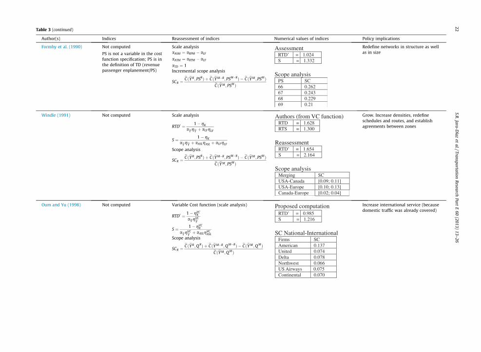
Table 3 (continued)

Author(s) Indices Reassessment of indices Numerical values of indices Policy implications

Formby et al. (1990) Not computed Scale analysis Redefine networks in structure as wellas in sizePS is not a variable in the cost

function specification; PS is inthe definition of TD (revenuepassenger enplanement/PS)

aASM ¼ aRPM � aLF

aATM ¼ aRTM � aLF

aTD ¼ 1Incremental scope analysis

SCR ¼eCðeY R; PSRÞ þ eCðeY M�R; PSM�RÞ � eCðeY M ; PSMÞeCðeY M ; PSMÞ

Windle (1991) Not computed Scale analysis Grow. Increase densities, redefineschedules and routes, and establishagreements between zonesRTD0 ¼ 1� gK

aeY geY þ aLFgLF

S ¼ 1� gK

aeY geY þ aASLgASL þ aLFgLF

Scope analysis

SCR ¼eCðeY R; PSRÞ þ eCðeY M�R; PSM�RÞ � eCðeY M ; PSMÞeCðeY M ; PSMÞ

Oum and Yu (1998) Not computed Variable Cost function (scale analysis) Increase international service (becausedomestic traffic was already covered)

RTD0 ¼ 1� gVCK

aeY gVCeYS ¼ 1� gVC

K

aeY gVCeY þ aASLgVCASL

Scope analysis

SCR ¼eCðeY R;QRÞ þ eCðeY M�R;QM�RÞ � eCðeY M ;QMÞeCðeY M ;QMÞ

Proposed computation RTD’ = 0.985 S = 1.216

SC National-International Firms SC American 0.137 United 0.074 Delta 0.078 Northwest 0.066 US Airways 0.075 Continental 0.070

Assessment RTD’ = 1.024 S = 1.332

Scope analysis PS SC 66 0.262 67 0.243 68 0.229 69 0.21

Authors (from VC function) RTD = 1.628 RTS = 1.300

Reassessment RTD’ = 1.654 S = 2.164

Scope analysis Merging SC USA-Canada [0.09; 0.11] USA-Europe [0.10; 0.13] Canada-Europe [0.02; 0.04]

22S.R

.Jara-Díaz

etal./Transportation

Research

PartE

60(2013)

13–26

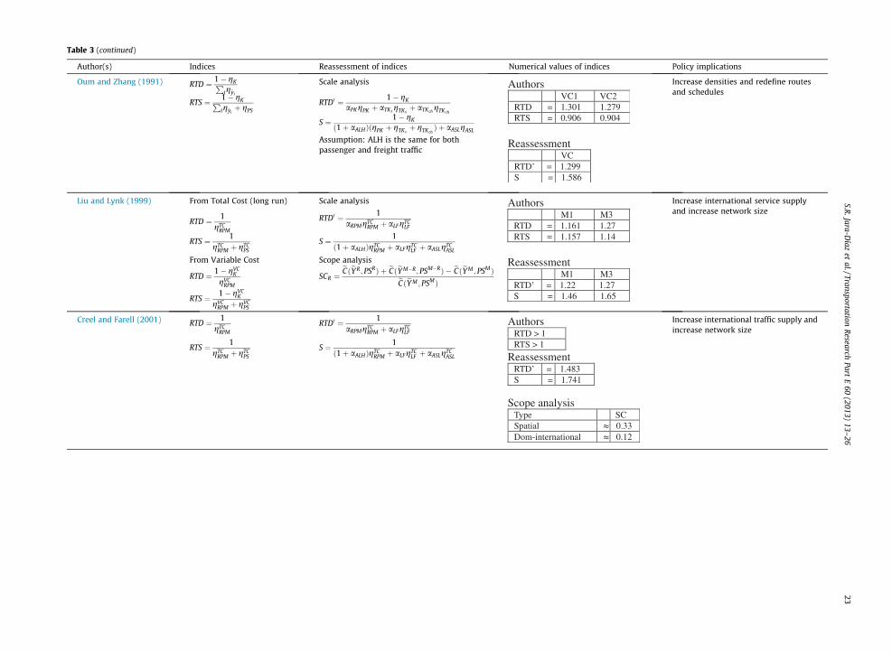
Table 3 (continued)

Author(s) Indices Reassessment of indices Numerical values of indices Policy implications

Oum and Zhang (1991) RTD ¼ 1� gKPig~yi

Scale analysis Increase densities and redefine routesand schedules

RTS ¼ 1� gKPig~yiþ gPS

RTD0 ¼ 1� gK

aPKgPK þ aTKs gTKsþ aTKch

gTKch

S ¼ 1� gK

ð1þ aALHÞðgPK þ gTKsþ gTKch

Þ þ aASLgASL

Assumption: ALH is the same for bothpassenger and freight traffic

Liu and Lynk (1999) From Total Cost (long run) Scale analysis Increase international service supplyand increase network size

RTD ¼ 1gTC

RPM

RTD0 ¼ 1aRPMgTC

RPM þ aLFgTCLF

RTS ¼ 1gTC

RPM þ gTCPS

S ¼ 1ð1þ aALHÞgTC

RPM þ aLFgTCLF þ aASLgTC

ASL

From Variable Cost Scope analysis

RTD ¼ 1� gVCK

gVCRPM

SCR ¼eCðeY R; PSRÞ þ eCðeY M�R; PSM�RÞ � eCðeY M ; PSMÞeCðeY M ; PSMÞ

RTS ¼ 1� gVCK

gVCRPM þ gVC

PS

Creel and Farell (2001) RTD ¼ 1gTC

RPM

RTD0 ¼ 1aRPMgTC

RPM þ aLFgTCLF

Increase international traffic supply andincrease network size

RTS ¼ 1gTC

RPM þ gTCPS

S ¼ 1ð1þ aALHÞgTC

RPM þ aLFgTCLF þ aASLgTC

ASL

Authors RTD > 1 RTS > 1

Reassessment RTD’ = 1.483 S = 1.741

Scope analysis Type SC Spatial 0.33 Dom-international 0.12

Authors VC1 VC2 RTD = 1.301 1.279 RTS = 0.906 0.904

Reassessment VC RTD’ = 1.299 S = 1.586

Authors M1 M3 RTD = 1.161 1.27 RTS = 1.157 1.14

Reassessment M1 M3 RTD’ = 1.22 1.27 S = 1.46 1.65

S.R.Jara-D

íazet

al./TransportationR

esearchPart

E60

(2013)13–

2623

24 S.R. Jara-Díaz et al. / Transportation Research Part E 60 (2013) 13–26

shown that irrespective of possibly increasing RTD (by itself an incentive to merge), the firms with small networks presentedincreasing returns to spatial scope, suggesting the convenience of expanding their networks at constant density. This lastobservation, along with our conclusions from the merging scope analysis, provides a solid explanation for the observed net-work expansion of small firms. Gillen et al. (1990) and Oum and Zhang (1991) obtained an RTS value close to one, from whichthey concluded that airline firms had a cost advantage to increase the flows on a fixed network, which was not observed fromthe 1980s onward. In reality, the small and medium-sized firms finally merged in 1987 to form Canadian Airlines to competewith Air Canada. The small firms disappeared after deregulation, consistent with our analyses based on economies of scopefor different partitions, corrected returns to density, and multioutput scale economies.

4. Synthesis and conclusions

Most of the analyses of airline industry structure have been performed using two scale-like concepts defined in the aggre-gates: returns to density (RTD), which considers output growth keeping network size (and route structure) constant, and re-turns to scale (RTS), which considers variations in the network size (number of points served). With these concepts, potentialcost savings arising from output and/or network growth have been studied, finding increasing returns to density and (typ-ically) constant returns to (network) scale. The explanations for the observed network growth have been based on densityalone. We have re-analyzed the issue using the detailed description of product as the starting point. As a result, we haveadvocated for the calculation of three indices:

– A new value for returns to density, RTD0, which is a recalculation of RTD based on some corrections to the aggregate out-put cost elasticities (Jara-Díaz and Cortés, 1996).

– The multiproduct degree of economies of scale, S, which relaxes the assumption of a fixed route structure implicit in thecomputation of RTD0, using a similar method with potentially different correction factors (Basso and Jara-Díaz, 2006a).

– Economies of spatial scope, SC (Basso and Jara-Díaz, 2005), which addresses the important issue of network size.

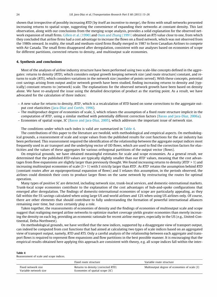
The conditions under which each index is valid are summarized in Table 4.The contributions of this paper to the literature are twofold, with methodological and empirical aspects. On methodolog-

ical grounds, a reassessment of scale and scope values from the published results for cost functions for the air industry hasbeen performed. This reassessment required the identification of the relationship between the aggregate output indices mostfrequently used in air transport and the underlying vector of OD flows, which are used to find the correction factors for elas-ticities and the values of these aggregates for various orthogonal partitions of the output vector (flows).

On empirical grounds, we have obtained meaningful estimates for scale and scope economies. As a general result, wedetermined that the published RTD values are typically slightly smaller than our RTD0 values, meaning that the cost advan-tages from flow expansions are slightly larger than previously thought. We found increasing returns to density (RTD0 > 1) andincreasing multioutput economies of scale (S > 1) with S strictly larger than RTD0. As RTD0 retains the assumption behind RTD(constant routes after an equiproportional expansion of flows) and S relaxes this assumption, in the periods observed, theairlines could diminish their costs to produce larger flows on the same network by restructuring the routes for optimaloperation.

Many types of positive SC are detected, including network size, trunk-local services, and domestic-international markets.Trunk-local scope economies contribute to the explanation of the cost advantages of hub-and-spoke configurations thatemerged after deregulation. The findings of domestic-international economies of scope are particularly appealing, as theyfall within the 5% savings calculated when using large US and world airlines and 12% when using US airlines only. Of course,there are other elements that should contribute to fully understanding the formation of powerful international alliancesremaining over time, but costs certainly play a role.

Taken together, the reassessments of economies of density and the findings of economies of multioutput scale and scopesuggest that realigning merged airline networks to optimize market coverage yields greater economies than merely increas-ing the density on each leg, providing an economic rationale for recent airline mergers, especially in the US (e.g., United-Con-tinental, Delta-Northwest).

On methodological grounds, we have verified that the new indices, supported by a disaggregate view of transport output,can indeed be computed from cost functions that had aimed at calculating two types of scale indices based on an aggregatedview of transport output, namely, RTD and RTS. Only a careful analysis of the relationship between each aggregate and trans-port flows is required to represent flow expansions and flow partitions in the best possible manner. It is encouraging that theempirical results obtained here applying this approach are consistent with theory, e.g. all scope indices fall within the inter-

Table 4Reassessment of scale and scope indices.

Fixed route structure Variable route structure

Fixed network size Returns to density (corrected RTD) Multioutput degree of economies of scale (S)Variable network size Economies of spatial scope (SC)

S.R. Jara-Díaz et al. / Transportation Research Part E 60 (2013) 13–26 25

val (-1, 1), and are appealing as a means to enlighten the analysis of the impact of output growth on costs in the airline indus-try structure by means of scale and scope.

Acknowledgments

This research was partially financed by Fondecyt, Chile, Grant 1120316, and the Institute of Complex Engineering Systems(Grants ICM: P-05-004-F and CONICYT: FB016). We thank Leonardo Basso for his comments and suggestions on earlier draftsof this paper and the referees. We particularly thank the referee who noted some significant evolutions in certain US airlinesregarding networks (route structures) and aircraft sizes. Remaining errors are the authors’ errors alone.

References

Baltagi, B., Griffin, J., Rich, D., 1995. Airline deregulation: the cost pieces of the puzzle. International Economic Review 36, 245–259.Basso, L., Jara-Díaz, S., 2005. Calculation of economies of spatial scope from transport cost functions with aggregate output (with an application to the airline

industry). Journal of Transport Economics and Policy 39 (1), 25–52.Basso, L., Jara-Díaz, S., 2006a. Distinguishing economies of density from economies of scale on a fixed-size transport network. Networks and Spatial

Economics 6 (2), 149–162.Basso, L., Jara-Díaz, S., 2006b. Is Returns to Scale with variable network size adequate for transport industry structure analysis? Transportation Science 40,

259–268.Borenstein, S., 1992. The evolution of U.S. airline competition. Journal of Economic Perspectives 6 (2), 45–73.Braeutigam, R., 1999. Learning about transport costs. In: Gomez-Ibañez, J., Tye, W., Winston, C. (Eds.), Essays in Transportation Economics and Policy.

Brooking Institution Press, USA, Washington, DC, pp. 57–97.Brueckner, J., Spiller, P., 1994. Economies of traffic density in the deregulated airline industry. The Journal of Law and Economics 37 (2), 379–413.Caves, D., Christensen, L., Tretheway, M., 1984. Economies of density versus economies of scale: why trunk and local airline costs differ. Rand Journal of

Economics 15, 471–489.Caves, D., Christensen, L., 1988. The importance of the economies of scale, capacity utilization and density in explaining interindustry differences in

productivity growth. Logistics and Transportation Review 2, 3–32.Creel, M., Farell, M., 2001. Economies of scale in the U.S. airline industry after deregulation: a fourier series approximation. Transportation Research Part E

37, 321–336.Daughety, A., 1985. Transportation research on pricing and regulation: overview and suggestions for future research. Transportation Research Part A 19 (5/

6), 471–487.Formby, J., Thistle, P., Keeler, J., 1990. Cost under regulation and deregulation: the case of US passengers airlines. The Economic Record 66, 308–321.Gagné, R., 1990. On the relevant elasticity estimates for cost structure analysis of the trucking industry. The Review of Economics and Statistics 72, 160–164.Gillen, D., Oum, T., Tretheway, M., 1990. Airline cost structure and policy implications. Journal of Transport Economics and Policy 24, 9–34.Hendricks, K., Piccione, M., Tan, G., 1995. The economics of hubs: the case of monopoly. Review of Economics Studies 62, 83–99.Hurdle, G., Johnson, R., Toskow, A., Warden, G., Williams, M., 1989. Concentration, potential entry and performance in the airline industry. Journal of

Industrial Economics 38 (2), 119–139.Jara-Díaz, S., 1982a. The estimation of transport cost functions: a methodological review. Transport Reviews, 257–278.Jara-Díaz, S., 1982b. Transportation product, transportation function and cost function. Transportation Science 16, 522–539.Jara-Díaz, S., 2007. Transport Economic Theory. Elsevier, Amsterdam.Jara-Díaz, S., Basso, L., 2003. Transport cost functions, network expansion and economies of scope. Transportation Research Part E 39 (4), 271–288.Jara-Díaz, S., Cortés, C., 1996. On the calculation of scale economies from transport cost functions. Journal of Transport Economics and Policy 30, 157–170.Jara-Díaz, S., Cortés, C., Ponce, F., 2001. Number of points served and economies of spatial scope in transport cost functions. Journal of Transport Economics

and Policy 35, 327–341.Johnston, A., Ozment, J., 2013. Economies of scale in the US airline industry. Transportation Research Part E 51, 95–108.Keeler, J., Formby, J., 1994. Cost economies and consolidation in the us airline industry. International Journal of Transport Economics 21 (1), 21–45.Kraus, M., 2008. Economies of scale in networks. Journal of Urban Economics 64, 171–177.Kumbhakar, S., 1990. A Reexamination of returns to scale, density and technical progress in USA. Southern Economics Journal 57 (2), 428–442.Liu, Z., Lynk, E., 1999. Evidence on Market structure of the deregulated us airline industry. Applied Economics 31, 1083–1092.Oum, T., Tretheway, M., 1990. Airline Hub and spoke system. Transportation Research Forum Proceedings 30, 380–393.Oum, T., Yu, C., 1998. Cost Competitiveness of mayor airlines: an international comparison. Transportation Research Part A 32 (6), 407–422.Oum, T., Zhang, Y., 1991. Utilisation of quasi-fixed inputs and estimation of cost functions. Journal of Transport Economics and Policy 25 (2), 121–134.Oum, T., Zhang, Y., 2000. A note on scale economies in transport. Journal of Transport Economics and Policy 31, 309–315.Oum, T., Park, J., Zhang, A., 2000. Globalization and Strategic Alliances: the Case of the Airline Industry. Elsevier Science, Pergamon, Oxford.Oum, T., Zhang, A., Zhang, Y., 1995. Airline network rivalry. Canadian Journal of Economics, 836–857.Panzar, J., Willig, R., 1977. Economies of scale in multioutput production. Quarterly Journal of Economics 91 (3), 481–493.Panzar, J., 1989. Technological Determinants of Firm and Industry Structure. In: Schmalensee, R., Willig, R. (Eds.). Handbook of Industrial Organization,

North-Holland, pp. 3–59.Spady, R., Friedlaender, A., 1978. Hedonic cost functions for the regulated trucking industry. Bell Journal of Economics 9, 59–179.Swan, W., 2002. Airline route developments: a review of history. Journal of Air Transport Management 8, 349–353.Wei, W., Hansen, M., 2003. Cost economics of aircraft size. Journal of Transport Economics and Policy 37, 279–296.Windle, R., 1991. The world’s airlines: a cost and productivity comparison. Journal of Transport Economics and Policy 25 (1), 31–49.Winston, C., 1985. Conceptual developments in the economics of transportation: an interpretive survey. Journal of Economic Literature 23, 57–94.Xu, K., Windle, R., Grimm, C., Corsi, T., 1994. Re-evaluating returns to scale in transport. Journal of Transport Economics and Policy 28, 275–286.Ying, J., 1992. On calculating cost elasticities. The Logistics and Transportation Review 28 (3), 231–235.

Glossary

General variableseY : Aggregate productN: Network indexQ: Product attributesK: Capitalu: Hedonic productW: Input price vector

26 S.R. Jara-Díaz et al. / Transportation Research Part E 60 (2013) 13–26

t: Time associated with technological changeT: Vector of time shiftsF: Vector of firm-specific shiftsA(t): Technical progress indexE: Efficiency indexu: Capital utilization rateIM: Multilateral indexg: Dummy variable representing government propertyv: Dummy variable capturing other effectsS: Capital stock flowD: Dummy variable indicating cost differences among firmsPS: Number of points servedCPS: City pairs servedAggregate products and attributesRPM: Revenue passenger milesRTM: Revenue ton milesRPK: Revenue passenger kilometersRTK: Revenue ton-kilometersASL: Average stage lengthLF: Load factorASM: Available seat-milesATM: Available ton-milesFSL: Flight stage lengthHub: Structure network indicatorTD: Traffic densityAU: Fleet utilizationALH: Average length of haul