Received February 9, 2021, accepted February 18, 2021, date of publication February 26, 2021, date of current version March 16, 2021. Digital Object Identifier 10.1109/ACCESS.2021.3062493 DeepKneeExplainer: Explainable Knee Osteoarthritis Diagnosis From Radiographs and Magnetic Resonance Imaging MD. REZAUL KARIM 1,2 , JIAO JIAO 3 , TILL DÖHMEN 1,2 , MICHAEL COCHEZ 4,6 , OYA BEYAN 1,2 , DIETRICH REBHOLZ-SCHUHMANN 5 , AND STEFAN DECKER 1,2 1 Fraunhofer Institute for Applied Information Technology (FIT), 53754 Sankt Augustin, Germany 2 Computer Science 5-Information Systems and Databases, RWTH Aachen University, D-52056 Aachen, Germany 3 Fraunhofer Institute for Systems and Innovation Research ISI, 76139 Karlsruhe, Germany 4 Department of Computer Science, Faculty of Sciences, Vrije Universiteit Amsterdam, 1081 HV Amsterdam, The Netherlands 5 ZB MED—Information Centre for Life Sciences, 50931 Cologne, Germany 6 Elsevier’s Discovery Lab, 1090 GH Amsterdam, The Netherlands Corresponding author: Md. Rezaul Karim (rezaul.karim@fit.fraunhofer.de) ABSTRACT Osteoarthritis (OA) is a degenerative joint disease, which significantly affects middle-aged and elderly people. Although primarily identified via hyaline cartilage change based on medical images, technical bottlenecks like noise, artifacts, and modality impose an enormous challenge on high-precision, objective, and efficient early quantification of OA. Owing to recent advancements, approaches based on neural networks (DNNs) have shown outstanding success in this application domain. However, due to nested non-linear and complex structures, DNNs are mostly opaque and perceived as black-box methods, which raises numerous legal and ethical concerns. Moreover, these approaches do not have the ability to provide the reasoning behind diagnosis decisions in the way humans would do, which poses an additional risk in the clinical setting. In this paper, we propose a novel explainable method for knee OA diagnosis based on radiographs and magnetic resonance imaging (MRI), which we called DeepKneeExplainer. First, we comprehensively preprocess MRIs and radiographs through the deep-stacked transformation technique against possible noises and artifacts that could contain unseen images for domain generalization. Then, we extract the region of interests (ROIs) by employing U-Net architecture with ResNet backbone. To classify the cohorts, we train DenseNet and VGG architectures on the extracted ROIs. Finally, we highlight class-discriminating regions using gradient-guided class activation maps (Grad-CAM++) and layer-wise relevance propagation (LRP), followed by providing human-interpretable explanations of the predictions. Comprehensive experiments based on the multicenter osteoarthritis study (MOST) cohorts, our approach yields up to 91% classification accuracy, outperforming comparable state-of-the-art approaches. We hope that our results will encourage medical researchers and developers to adopt explainable methods and DNN-based analytic pipelines towards an increasing acceptance and adoption of AI-assisted applications in the clinical practice for improved knee OA diagnoses. INDEX TERMS Knee osteoarthritis, biomedical imaging, deep neural networks, neural ensemble, explain- ability, Grad-CAM++, layer-wise relevance propagation. I. INTRODUCTION Osteoarthritis (OA) is a degenerative joint disease, which is defined as a heterogeneous group of health conditions and a phenomenal chronic disease. OA leads to joint symptoms and The associate editor coordinating the review of this manuscript and approving it for publication was Qi Zhou. signs associated with defective integrity of articular cartilage, associated with changes in the underlying bone at the joint margins [1]. OA can affect joints, often in knees, hips, lower back and neck, small joints of the fingers, and bases of the thumbs and big toes [2]. The increasing prevalence of OA has not only posed an enormous challenge for the health of middle-aged and elderly but also tends to affect younger VOLUME 9, 2021 This work is licensed under a Creative Commons Attribution-NonCommercial-NoDerivatives 4.0 License. For more information, see https://creativecommons.org/licenses/by-nc-nd/4.0/ 39757

Welcome message from author
This document is posted to help you gain knowledge. Please leave a comment to let me know what you think about it! Share it to your friends and learn new things together.
Transcript
Received February 9, 2021, accepted February 18, 2021, date of publication February 26, 2021, date of current version March 16, 2021.
Digital Object Identifier 10.1109/ACCESS.2021.3062493
DeepKneeExplainer: Explainable KneeOsteoarthritis Diagnosis From Radiographs andMagnetic Resonance ImagingMD. REZAUL KARIM 1,2, JIAO JIAO3, TILL DÖHMEN 1,2, MICHAEL COCHEZ 4,6,OYA BEYAN 1,2, DIETRICH REBHOLZ-SCHUHMANN 5, AND STEFAN DECKER 1,21Fraunhofer Institute for Applied Information Technology (FIT), 53754 Sankt Augustin, Germany2Computer Science 5-Information Systems and Databases, RWTH Aachen University, D-52056 Aachen, Germany3Fraunhofer Institute for Systems and Innovation Research ISI, 76139 Karlsruhe, Germany4Department of Computer Science, Faculty of Sciences, Vrije Universiteit Amsterdam, 1081 HV Amsterdam, The Netherlands5ZB MED—Information Centre for Life Sciences, 50931 Cologne, Germany6Elsevier’s Discovery Lab, 1090 GH Amsterdam, The Netherlands
Corresponding author: Md. Rezaul Karim ([email protected])
ABSTRACT Osteoarthritis (OA) is a degenerative joint disease, which significantly affects middle-agedand elderly people. Although primarily identified via hyaline cartilage change based on medical images,technical bottlenecks like noise, artifacts, and modality impose an enormous challenge on high-precision,objective, and efficient early quantification of OA. Owing to recent advancements, approaches based onneural networks (DNNs) have shown outstanding success in this application domain. However, due to nestednon-linear and complex structures, DNNs are mostly opaque and perceived as black-box methods, whichraises numerous legal and ethical concerns. Moreover, these approaches do not have the ability to providethe reasoning behind diagnosis decisions in the way humans would do, which poses an additional risk inthe clinical setting. In this paper, we propose a novel explainable method for knee OA diagnosis basedon radiographs and magnetic resonance imaging (MRI), which we called DeepKneeExplainer. First,we comprehensively preprocess MRIs and radiographs through the deep-stacked transformation techniqueagainst possible noises and artifacts that could contain unseen images for domain generalization. Then,we extract the region of interests (ROIs) by employing U-Net architecture with ResNet backbone. To classifythe cohorts, we train DenseNet and VGG architectures on the extracted ROIs. Finally, we highlightclass-discriminating regions using gradient-guided class activation maps (Grad-CAM++) and layer-wiserelevance propagation (LRP), followed by providing human-interpretable explanations of the predictions.Comprehensive experiments based on the multicenter osteoarthritis study (MOST) cohorts, our approachyields up to 91% classification accuracy, outperforming comparable state-of-the-art approaches. We hopethat our results will encourage medical researchers and developers to adopt explainable methods andDNN-based analytic pipelines towards an increasing acceptance and adoption of AI-assisted applicationsin the clinical practice for improved knee OA diagnoses.
INDEX TERMS Knee osteoarthritis, biomedical imaging, deep neural networks, neural ensemble, explain-ability, Grad-CAM++, layer-wise relevance propagation.
I. INTRODUCTIONOsteoarthritis (OA) is a degenerative joint disease, which isdefined as a heterogeneous group of health conditions and aphenomenal chronic disease. OA leads to joint symptoms and
The associate editor coordinating the review of this manuscript andapproving it for publication was Qi Zhou.
signs associated with defective integrity of articular cartilage,associated with changes in the underlying bone at the jointmargins [1]. OA can affect joints, often in knees, hips, lowerback and neck, small joints of the fingers, and bases of thethumbs and big toes [2]. The increasing prevalence of OAhas not only posed an enormous challenge for the healthof middle-aged and elderly but also tends to affect younger
VOLUME 9, 2021This work is licensed under a Creative Commons Attribution-NonCommercial-NoDerivatives 4.0 License.
For more information, see https://creativecommons.org/licenses/by-nc-nd/4.0/ 39757
M. R. Karim et al.: DeepKneeExplainer: Explainable Knee OA Diagnosis From Radiographs and Magnetic Resonance Imaging
people with risk factors such as obesity and reduced physi-cal activity [3]. Being ranked 13th highest global disabilityfactor [4], OA places a high economic burden on society,in consideration of work absenteeism, early retirement, andjoint replacement [5]. Although the cost began to shrinkas of 2015, due to recent technical advances, an estimatedexpenditure per patient for joint replacement still reaches19,715 EUR per year [3].
Nevertheless, the costs arise, to a great extent, from the cur-rent clinical inability to systematically diagnose the disease atan early stage [6]. However, early diagnosis remains the pri-mary option to prolong the patient’s health in a cost-effectivemanner and the identification of hyaline-cartilage changeon medical images stands as the primary method for saiddiagnosis. The process of measuring cartilage morphologyis a time-consuming process, especially when utilizing MRI.A manual analysis of a 3D knee MRI sequence takes up to6 hours for trained surgeons [7]. An AI-guided diagnosticpipeline could support experts in the process, while drasti-cally reducing the time required for OA grading, and allowingsurgeons or radiologists to dedicate more of their valuabletime to more acute tasks.
Early detection of OA and subsequent prognosis becamemore prevalent and feasible with the rise of digital med-ical imaging [2]. Available biomedical imaging modali-ties include ultrasound, mammograms, X-ray, computedtomography (CT), magnetic resonance imaging (MRI),electroencephalography, electrocardiography, endoscopy,elastography, magnetoencephalography, tactile imaging,thermograph, and nuclear medicine functional imaging [8].CT and radiographs exhibit bone shapes well but carry lessinformation on soft-tissue regions, which can be important forOA diagnosis [9], [10]. MRIs, in turn, are particularly usefulfor the identification of full or partial-thickness changes ofarticular cartilage, but can not capture bone architectureswell, which are a potential indicator for an earliest OAprogression [2], [9], [11]. Accurate analysis of biomedicalimaging not only dependent on feature extraction but alsosegmentation [12], [13].
Therefore, each modality on its own may hence not con-tain sufficient information for an accurate OA quantifica-tion or diagnosis. Further, artifacts such as aliasing, sliceoverlap, truncation, patient motion, and pathological featureslike osteophytes, bone marrow lesions, and surface fibril-lation also impede accurate diagnosis of OA [14]. Deeplearning (DL) techniques propelled recent advancements incomputer vision techniques which again lead to a rise inautomated medical diagnoses solutions and computer-aidedclinical decision-making [15]. However, the reliability ofmany existing approaches that solely focus on segmentationor classification accuracy can be questioned due to severalreasons [16]. Nevertheless, due to the nested non-linear andcomplex structures, DNNs are mostly perceived as ‘‘blackbox" methods [16], which raises numerous legal and ethicalconcerns, especially for clinical applications.
In order to improve the effectiveness of the OA diag-nosis and the interpretability, which are impeded by theuse of single modalities and a lack of explainability, ourstudy establishes a comparative quantification of multipleperspectives of radiographs and MRIs to provide explain-able diagnoses. We propose a novel OA quantificationand diagnosis solution based on explainable neural ensem-ble methods, which we call DeepKneeExplainer. Thediagnosis pipeline of DeepKneeExplainer consists ofa deep-stacked transformation-based image preprocessingstep, ROI extraction, classification, multimodality integra-tion, and decision visualization.
First, we comprehensively preprocess both MRIs andradiographs through the deep-stacked transformation tech-nique against possible noises and artifacts that could containunseen images for domain generalization. Then, to detectand localize knee joints from different perspectives of X-rayimages, we employed U-Net with different ResNet back-bones in which ROIs are detected with a faster region con-volutional neural network (FRCNN) by optimizing binarycross-entropy (BCE) and intersection over union (IoU) losses.On the other hand, VGGNet and DenseNet architectures areused
The rest of the paper is structured as follows: Section IIcovers related work on knee OA quantification and automaticdiagnosis and points out potential limitations. Section IIIdescribes our proposed approach outlining data preprocess-ing, network constructions, training, and decision visualiza-tions. Section IV demonstrates experiment results and dis-cusses the key findings of the study. Section V summarizesthe work and identifies potential limitations, before conclud-ing the paper.
II. RELATED WORKDifferent modalities have a predominant influence on accu-rate quantification and long-term prognosis of OA. Hence,we discuss in detail automatic OA quantification criteria andmechanisms covering radiographs and MRI.
A. RADIOGRAPHSWhile different 3D modality perspectives have emergedrecently, conventional radiographs are still widely used, espe-cially due to their availability and low-costs [17]. Radio-graphs exhibit potential for displaying bone shape OA fea-tures, e.g., osteophytes, Joint Space Width (JSW) narrowing,subchondral sclerosis, and cysts rather than adjacent tissues,which are more explicit characteristics for OA. This par-ticularly holds for the early-stage detection [9], [18], whilethe pathological changes are associated with severe stagesof OA [18], [19]. However, due to the projection nature,radiography is limited to the detection of subtle changesin the longitudinally and stereoscopic space. Incorporatingmore perspectives into the examination process is expectedto increase the likelihood of correct knee OA diagnoses [20].
39758 VOLUME 9, 2021
M. R. Karim et al.: DeepKneeExplainer: Explainable Knee OA Diagnosis From Radiographs and Magnetic Resonance Imaging
1) EVALUATION CRITERIADue to difficulties in measurement, interpretation, andsemi-quantitative grading systems in automatic knee OAdetection, quantitative grading systems such as Kellgren andLawrence (KL) or the osteoarthritis research society inter-national atlas (OARSI) are most common. KL scale definesradiographic OA with a global composite score on a rangefrom 0-4 [21] and reflects an incremental severity of OA.KL grade 0 signifies no presence of OA and grade 4 indicatesserious OA [22], while grade 1 is doubtful narrowing, grade2 is possible narrowing, and grade 3 signifies a definitenarrowing of joint space. Employing KL grading systemfor progression description has entailed additional risks forautomatic OA quantification, since KL grade 3 encompassesall degrees of JSN, regardless of the actual extent [23],[24]. Moreover, knees at KL grade 4 that exhibit a bone-on-bone appearance are still prone to structural changes,e.g., bone marrow lesions, effusion, synovitis, and Hoffa-synovitis, which can only be detected on MRIs [23], [24],making ‘‘end-stage" not equivalent to KL grade 4, where amodified KL definition arises from [25].
The OARSI atlas provides image examples for particulargrades and specific features of OA rather than assigningglobal scores [24] and acts as an alternative to KL grading.The OARSI atlas scores tibiofemoral JSN and osteophytesseparately for each knee compartment in which the medial,lateral, and patellofemoral are each graded on a 0-3 scale:grade 0 represents a normal knee joint, grade 1 a mildknee joint, grade 2 a moderate/mild knee joint, and grade3 signifies severe knee joint condition. KL grading systemis more widely used for automatic OA detection. However,due to its evaluation convenience, the OARSI JSN gradingsystem leads to higher confidence levels in the computer-aiddiagnosis task due to richer training data [23], [25], [26].
2) QUANTIFICATION WORKFLOWSROI detection, extraction, and subsequent classification (i.e.,ROI extraction + classification) and end-to-end classifica-tion, which combines these steps into a single architecture,are two popular approaches for OA quantification followed inthe scientific literature. Although some approaches, e.g., [6],[27] achieved a precision of 0.7, OA quantification accuracyis approaching a bottleneck, which cannot simply be over-come with a better choice of evaluation criteria or workflows,if they are solely based on plain radiographs.
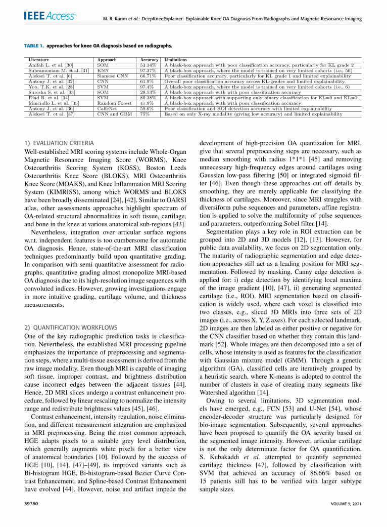
Several approaches for feature extraction are presented inthe literature, e.g., Yoo et al. [28] compute kinematic factorsand use them as features, which are then classified with sup-port vector machines (SVM), yielding an accuracy of 97.4%.Furthermore, Naïve Bayes (NB), Radial Basis Func-tion (RBF) networks, and random forest (RF) are utilizedand attained comparable accuracy [29]. Anifah et al. [30]applied the gray-level co-occurrence matrix (GLCM) withGabor kernel, giving an accuracy of 53.34%. However, only
4% of the radiographs could correctly be classified as KLgrade 2. Subramoniam et al. [31] used the central joint regionas ROI and extracted the features manually, followed by aK-Nearest Neighbor (KNN) for the classification.
Although their approach achieved an accuracy of 95%,the ROI extraction is not robust. Besides, it lacks scien-tific evidence, given that the evaluation was carried outon very limited cohorts. Therefore, due to the shortcom-ings of ML-based approaches, extensive exploration of DLemerged for knee OA analysis and quantification, followedby wavelet transformation of images, Restricted BoltzmannMachine (RBM) for feature extraction. Subsequently, fullyautomated OA quantization based on DNNs emerged. Inparticular, convolutional neural networks (CNN) are widelyused to extract more abstract and salient features, whereboth ROI detection, extraction, and classification are inte-grated into a single pipeline. Antony et al. [36] employedlinear SVM with the Sobel horizontal image gradients todetect knee joints and fine-tuned pre-trained BVLC Caf-feNet and VGG-M-128 models on OAI cohorts. The qualityof the ROI extraction is then evaluated by measuring theJaccard index or IoU, i.e., by computing matching scoresbetween manual annotations and automatic extraction, givinga Jaccard index of 0.36. While a CNN trained on OAI andMOST data sets, reportedly achieved a mean Jaccard indexof 0.83 only [32].
Approach [35] based on a 6-layer trained CNN achieveda 62% accuracy, while the gap between automatic and man-ual localization narrowed down from 4% to 2%. Besides,SVM-based scoring for gradually modifying was proposedfor ROIs extraction in which a Siamese CNN is trainedto detect lateral and medial sides of knee joints [6]. Otherapproaches [38], [39] employed ensemble Grad-CAM onSiamese networks to automatically highlight important fea-tures, giving an accuracy of 66.71%. Despite promisingresults, these approaches (as shown in table 1) could not fulfillclinical requirements. Aleksei T. et al. [6] proposed a multi-modal approach by utilizing radiographs, physical examina-tion, medical history, anthropometric data, and radiologist’sKL-grades to predict structural OA progression, followed bythe OA progression evaluation jointly with the current OAseverity in the analyzed knee, as an auxiliary outcome. Theyattempted to improve the CNN-based prognosis by fusingthe prediction with the clinical data with gradient boostingmachines (GBM).
B. MAGNETIC RESONANCE IMAGINGAs a non-invasive modality with high spatial resolution with-out ionizing radiation and multi-planar capability, MRI cancapture useful structures of the joint, e.g., cartilage mor-phology and biochemical composition [40], [41]. On theother hand, MRI is very sensitive to full or partial-thicknesschanges of articular cartilage over time, albeit it cannot depictclear bone architectures. This is similar to technical charac-teristics of radiography [2], [9].
VOLUME 9, 2021 39759
M. R. Karim et al.: DeepKneeExplainer: Explainable Knee OA Diagnosis From Radiographs and Magnetic Resonance Imaging
TABLE 1. approaches for knee OA diagnosis based on radiographs.
1) EVALUATION CRITERIAWell-established MRI scoring systems include Whole-OrganMagnetic Resonance Imaging Score (WORMS), KneeOsteoarthritis Scoring System (KOSS), Boston LeedsOsteoarthritis Knee Score (BLOKS), MRI OsteoarthritisKnee Score (MOAKS), and Knee InflammationMRI ScoringSystem (KIMRISS), among which WORMS and BLOKShave been broadly disseminated [24], [42]. Similar to OARSIatlas, other assessments approaches highlight spectrum ofOA-related structural abnormalities in soft tissue, cartilage,and bone in the knee at various anatomical sub-regions [43].
Nevertheless, integration over articular surface regionsw.r.t. independent features is too cumbersome for automaticOA diagnosis. Hence, state-of-the-art MRI classificationtechniques predominantly build upon quantitative grading.In comparison with semi-quantitative assessment for radio-graphs, quantitative grading almost monopolize MRI-basedOA diagnosis due to its high-resolution image sequences withconvoluted indices. However, growing investigations engagein more intuitive grading, cartilage volume, and thicknessmeasurements.
2) QUANTIFICATION WORKFLOWSOne of the key radiographic prediction tasks is classifica-tion. Nevertheless, the established MRI processing pipelineemphasizes the importance of preprocessing and segmenta-tion steps, where amulti-tissue assessment is derived from theraw image modality. Even though MRI is capable of imagingsoft tissue, improper contrast, and brightness distributioncause incorrect edges between the adjacent tissues [44].Hence, 2D MRI slices undergo a contrast enhancement pro-cedure, followed by linear rescaling to normalize the intensityrange and redistribute brightness values [45], [46].
Contrast enhancement, intensity regulation, noise elimina-tion, and different measurement integration are emphasizedin MRI preprocessing. Being the most common approach,HGE adapts pixels to a suitable grey level distribution,which generally augments white pixels for a better viewof anatomical boundaries [10]. Followed by the success ofHGE [10], [14], [47]–[49], its improved variants such asBi-histogram HGE, Bi-histogram-based Bezier Curve Con-trast Enhancement, and Spline-based Contrast Enhancementhave evolved [44]. However, noise and artifact impede the
development of high-precision OA quantization for MRI,give that several preprocessing steps are necessary, such asmedian smoothing with radius 1*1*1 [45] and removingunnecessary high-frequency edges around cartilages usingGaussian low-pass filtering [50] or integrated sigmoid fil-ter [46]. Even though these approaches cut off details bysmoothing, they are merely applicable for classifying thethickness of cartilages. Moreover, since MRI struggles withdiversiform pulse sequences and parameters, affine registra-tion is applied to solve the multiformity of pulse sequencesand parameters, outperforming Sobel filter [14].
Segmentation plays a key role in ROI extraction can begrouped into 2D and 3D models [12], [13]. However, forpublic data availability, we focus on 2D segmentation only.The maturity of radiographic segmentation and edge detec-tion approaches still act as a leading position for MRI seg-mentation. Followed by masking, Canny edge detection isapplied for: i) edge detection by identifying local maximaof the image gradient [10], [47], ii) generating segmentedcartilage (i.e., ROI). MRI segmentation based on classifi-cation is widely used, where each voxel is classified intotwo classes, e.g., sliced 3D MRIs into three sets of 2Dimages (i.e., across X, Y, Z axes). For each selected landmark,2D images are then labeled as either positive or negative forthe CNN classifier based on whether they contain this land-mark [52]. Whole images are then decomposed into a set ofcells, whose intensity is used as features for the classificationwith Gaussian mixture model (GMM). Through a geneticalgorithm (GA), classified cells are iteratively grouped bya heuristic search, where K-means is adopted to control thenumber of clusters in case of creating many segments likeWatershed algorithm [14].
Owing to several limitations, 3D segmentation mod-els have emerged, e.g., FCN [53] and U-Net [54], whoseencoder-decoder structure was particularly designed forbio-image segmentation. Subsequently, several approacheshave been proposed to quantify the OA severity based onthe segmented image intensity. However, articular cartilageis not the only determinate factor for OA quantification.S. Kubakaddi et al. attempted to quantify segmentedcartilage thickness [47], followed by classification withSVM that achieved an accuracy of 86.66% based on15 patients still has to be verified with larger subtypesample sizes.
39760 VOLUME 9, 2021
M. R. Karim et al.: DeepKneeExplainer: Explainable Knee OA Diagnosis From Radiographs and Magnetic Resonance Imaging
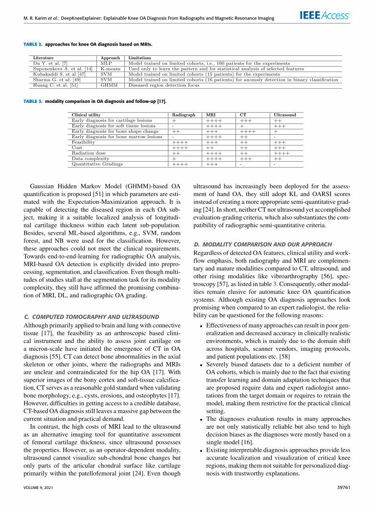
TABLE 2. approaches for knee OA diagnosis based on MRIs.
TABLE 3. modality comparison in OA diagnosis and follow-up [17].
Gaussian Hidden Markov Model (GHMM)-based OAquantification is proposed [51] in which parameters are esti-mated with the Expectation-Maximization approach. It iscapable of detecting the diseased region in each OA sub-ject, making it a suitable localized analysis of longitudi-nal cartilage thickness within each latent sub-population.Besides, several ML-based algorithms, e.g., SVM, randomforest, and NB were used for the classification. However,these approaches could not meet the clinical requirements.Towards end-to-end-learning for radiographic OA analysis,MRI-based OA detection is explicitly divided into prepro-cessing, segmentation, and classification. Even though multi-tudes of studies stall at the segmentation task for its modalitycomplexity, they still have affirmed the promising combina-tion of MRI, DL, and radiographic OA grading.
C. COMPUTED TOMOGRAPHY AND ULTRASOUNDAlthough primarily applied to brain and lung with connectivetissue [17], the feasibility as an arthroscopic based clini-cal instrument and the ability to assess joint cartilage ona micron-scale have initiated the emergence of CT in OAdiagnosis [55]. CT can detect bone abnormalities in the axialskeleton or other joints, where the radiographs and MRIsare unclear and contraindicated for the hip OA [17]. Withsuperior images of the bony cortex and soft-tissue calcifica-tion, CT serves as a reasonable gold standard when validatingbone morphology, e.g., cysts, erosions, and osteophytes [17].However, difficulties in getting access to a credible database,CT-based OA diagnosis still leaves amassive gap between thecurrent situation and practical demand.
In contrast, the high costs of MRI lead to the ultrasoundas an alternative imaging tool for quantitative assessmentof femoral cartilage thickness, since ultrasound possessesthe properties. However, as an operator-dependent modality,ultrasound cannot visualize sub-chondral bone changes butonly parts of the articular chondral surface like cartilageprimarily within the patellofemoral joint [24]. Even though
ultrasound has increasingly been deployed for the assess-ment of hand OA, they still adopt KL and OARSI scoresinstead of creating amore appropriate semi-quantitative grad-ing [24]. In short, neither CT nor ultrasound yet accomplishedevaluation-grading criteria, which also substantiates the com-patibility of radiographic semi-quantitative criteria.
D. MODALITY COMPARISON AND OUR APPROACHRegardless of detected OA features, clinical utility and work-flow emphasis, both radiography and MRI are complemen-tary and mature modalities compared to CT, ultrasound, andother rising modalities like vibroarthrography [56], spec-troscopy [57], as listed in table 3. Consequently, other modal-ities remain elusive for automatic knee OA quantificationsystems. Although existing OA diagnosis approaches lookpromising when compared to an expert radiologist, the relia-bility can be questioned for the following reasons:
• Effectiveness ofmany approaches can result in poor gen-eralization and decreased accuracy in clinically realisticenvironments, which is mainly due to the domain shiftacross hospitals, scanner vendors, imaging protocols,and patient populations etc. [58]
• Severely biased datasets due to a deficient number ofOA cohorts, which is mainly due to the fact that existingtransfer learning and domain adaptation techniques thatare proposed require data and expert radiologist anno-tations from the target domain or requires to retrain themodel, making them restrictive for the practical clinicalsetting.
• The diagnoses evaluation results in many approachesare not only statistically reliable but also tend to highdecision biases as the diagnoses were mostly based on asingle model [16].
• Existing interpretable diagnosis approaches provide lessaccurate localization and visualization of critical kneeregions, making them not suitable for personalized diag-nosis with trustworthy explanations.
VOLUME 9, 2021 39761
M. R. Karim et al.: DeepKneeExplainer: Explainable Knee OA Diagnosis From Radiographs and Magnetic Resonance Imaging
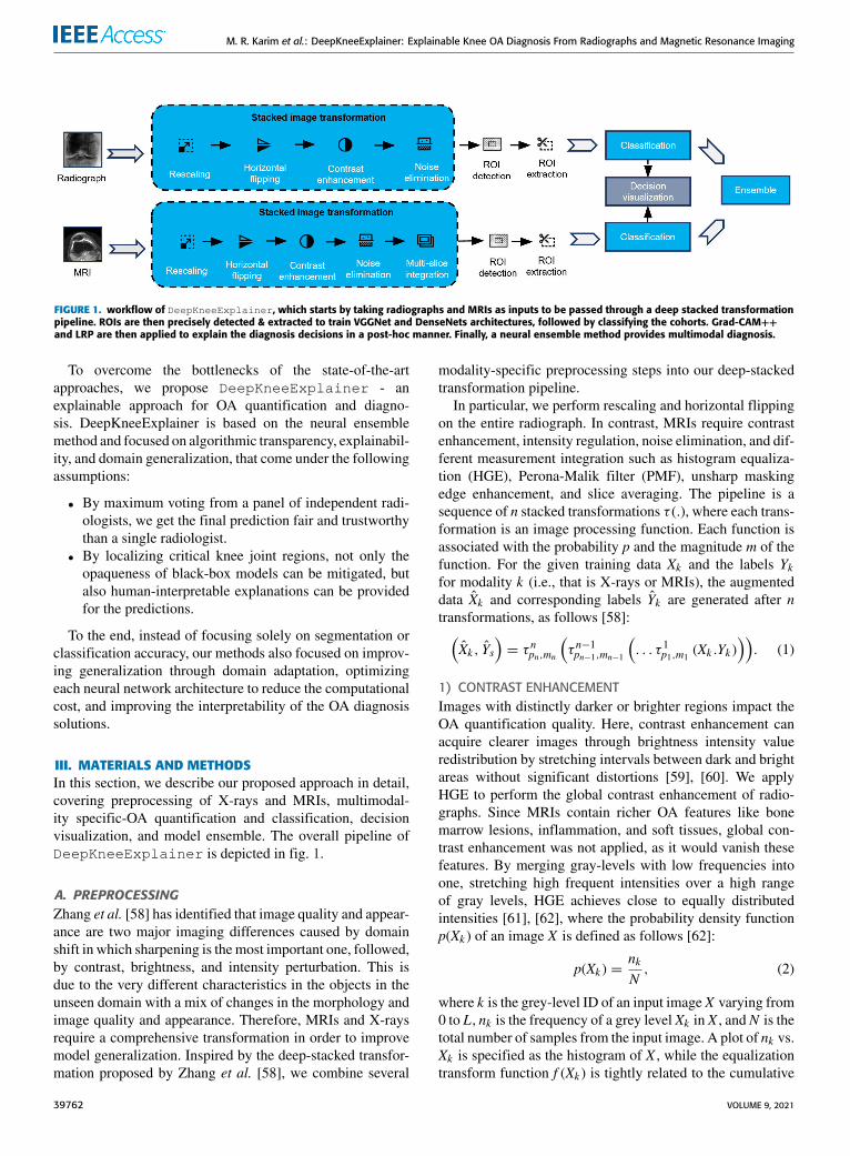
FIGURE 1. workflow of DeepKneeExplainer, which starts by taking radiographs and MRIs as inputs to be passed through a deep stacked transformationpipeline. ROIs are then precisely detected & extracted to train VGGNet and DenseNets architectures, followed by classifying the cohorts. Grad-CAM++
and LRP are then applied to explain the diagnosis decisions in a post-hoc manner. Finally, a neural ensemble method provides multimodal diagnosis.
To overcome the bottlenecks of the state-of-the-artapproaches, we propose DeepKneeExplainer - anexplainable approach for OA quantification and diagno-sis. DeepKneeExplainer is based on the neural ensemblemethod and focused on algorithmic transparency, explainabil-ity, and domain generalization, that come under the followingassumptions:
• By maximum voting from a panel of independent radi-ologists, we get the final prediction fair and trustworthythan a single radiologist.
• By localizing critical knee joint regions, not only theopaqueness of black-box models can be mitigated, butalso human-interpretable explanations can be providedfor the predictions.
To the end, instead of focusing solely on segmentation orclassification accuracy, our methods also focused on improv-ing generalization through domain adaptation, optimizingeach neural network architecture to reduce the computationalcost, and improving the interpretability of the OA diagnosissolutions.
III. MATERIALS AND METHODSIn this section, we describe our proposed approach in detail,covering preprocessing of X-rays and MRIs, multimodal-ity specific-OA quantification and classification, decisionvisualization, and model ensemble. The overall pipeline ofDeepKneeExplainer is depicted in fig. 1.
A. PREPROCESSINGZhang et al. [58] has identified that image quality and appear-ance are two major imaging differences caused by domainshift in which sharpening is themost important one, followed,by contrast, brightness, and intensity perturbation. This isdue to the very different characteristics in the objects in theunseen domain with a mix of changes in the morphology andimage quality and appearance. Therefore, MRIs and X-raysrequire a comprehensive transformation in order to improvemodel generalization. Inspired by the deep-stacked transfor-mation proposed by Zhang et al. [58], we combine several
modality-specific preprocessing steps into our deep-stackedtransformation pipeline.
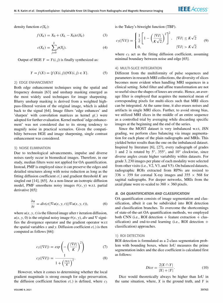
In particular, we perform rescaling and horizontal flippingon the entire radiograph. In contrast, MRIs require contrastenhancement, intensity regulation, noise elimination, and dif-ferent measurement integration such as histogram equaliza-tion (HGE), Perona-Malik filter (PMF), unsharp maskingedge enhancement, and slice averaging. The pipeline is asequence of n stacked transformations τ (.), where each trans-formation is an image processing function. Each function isassociated with the probability p and the magnitude m of thefunction. For the given training data Xk and the labels Ykfor modality k (i.e., that is X-rays or MRIs), the augmenteddata Xk and corresponding labels Yk are generated after ntransformations, as follows [58]:(
Xk , Ys)= τ npn,mn
(τ n−1pn−1,mn−1
(. . . τ 1p1,m1
(Xk .Yk))). (1)
1) CONTRAST ENHANCEMENTImages with distinctly darker or brighter regions impact theOA quantification quality. Here, contrast enhancement canacquire clearer images through brightness intensity valueredistribution by stretching intervals between dark and brightareas without significant distortions [59], [60]. We applyHGE to perform the global contrast enhancement of radio-graphs. Since MRIs contain richer OA features like bonemarrow lesions, inflammation, and soft tissues, global con-trast enhancement was not applied, as it would vanish thesefeatures. By merging gray-levels with low frequencies intoone, stretching high frequent intensities over a high rangeof gray levels, HGE achieves close to equally distributedintensities [61], [62], where the probability density functionp(Xk ) of an image X is defined as follows [62]:
p(Xk ) =nkN, (2)
where k is the grey-level ID of an input image X varying from0 to L, nk is the frequency of a grey level Xk in X , andN is thetotal number of samples from the input image. A plot of nk vs.Xk is specified as the histogram of X , while the equalizationtransform function f (Xk ) is tightly related to the cumulative
39762 VOLUME 9, 2021
M. R. Karim et al.: DeepKneeExplainer: Explainable Knee OA Diagnosis From Radiographs and Magnetic Resonance Imaging
density function c(Xk ):
f (Xk ) = X0 + (XL − X0)c(Xk ) (3)
c(Xk ) =k∑j=0
p(Xj). (4)
Output of HGE Y = Y (i, j) is finally synthesized as:
Y = f (X ) = {f (X (i, j))|∀X (i, j) ∈ X}. (5)
2) EDGE ENHANCEMENTBoth edge enhancement techniques using the spatial andfrequency domain [63] and unsharp masking emerged asthe most widely used techniques for image sharpening.Blurry unsharp masking is derived from a weighted high-pass-filtered version of the original image, which is addedback to the signal [64]. Image filters ’edge enhances’ and’sharpen’ with convolution matrices as kernel g(.) wereadopted for further evaluation. Kernel method ’edge enhance-ment’ was not considered due to its strong tendency tomagnify noise in practical scenarios. Given the compati-bility between HGE and image sharpening, single contrastenhancement was considered.
3) NOISE ELIMINATIONDue to technological advancements, impulse and diversenoises rarely occur in biomedical images. Therefore, in ourstudy, median filters were not applied for OA quantification.Instead, PMF is employed since it can preserve the edges anddetailed structures along with noise reduction as long as thefitting diffusion coefficient c(.) and gradient threshold K aresingled out [14], [65]. As a non-linear an-isotropic diffusionmodel, PMF smoothens noisy images θ (x, y) w.r.t. partialderivative [65]:
∂u∂t= div(c(|∇u(x, y, t)|)∇u(x, y, t)), (6)
where u(x, y, t) is the filtered image after t iteration diffusion,u(x, y, 0) is the original noisy image θ (x, y), div and ∇ signi-fies the divergence operator and the gradient operator w.r.tthe spatial variables x and y. Diffusion coefficient c(.) is thencomputed as follows [66]:
c1(|∇I |) = exp
(−
(|∇I |K
)2)
(7)
c2(|∇I |) =1
1+(|∇I |K
)2 . (8)
However, when it comes to determining whether the localgradient magnitude is strong enough for edge preservation,the diffusion coefficient function c(.) is defined, where c3
is the Tukey’s biweight function (TBF).
c3(|∇I |) =
12
[1−
(|∇I |
K√2
)2]2, |∇I | ≤ K
√2
0, |∇I | > K√2
(9)
where c3 act as the fitting diffusion coefficient, assumingminimal boundary between noise and edge [65].
4) MULTI-SLICE INTEGRATIONDifferent from the multiformity of pulse sequences andparameters in researchMRI collections, the diversity of slicesbecomes more evident when handling MRI sequences in aclinical setting. Sobel filter and affine transformation are notso useful since the shapes of knees are erratic. Hence, an aver-age filter is employed that acquires the numerical mean ofcorresponding pixels for multi-slices such that MRI slicescan be integrated. At the same time, it also erases noises andartifacts in single MRI slices. Further, to avoid strong bias,we utilized MRI slices in the middle of an entire sequenceas a controlled trial by averaging while discarding specificimages at the beginning and the end of the series.
Since the MOST dataset is very imbalanced w.r.t, JSNgrading, we perform class balancing via image augmenta-tion for each plane of the plain radiographs and MRIs. Thisyielded better results than the one on the imbalanced dataset.Inspired by literature [6], [27], every radiograph of grades1 and 2 is rotated by 5◦, 355◦, and 10◦ clockwise, sincediverse angles create higher variability within datasets. Forgrade 3, 230 images per plane of each modality were selectedfrom other visits (i.e., V2, V3, and V5). On balanced datasets,radiographic ROIs extracted from RPNs are resized to336 × 359 for coronal X-ray images and 355 × 568 forsagittal radiographs. For deeper networks, MRIs from theaxial plane were re-scaled to 360 × 360 pixels.
B. OA QUANTIFICATION AND CLASSIFICATIONOA quantification consists of image segmentation and clas-sification, albeit it can be subdivided into ROI detectionand classification branches. To overcome the shortcomingsof state-of-the-art OA quantification methods, we employedboth CNN (i.e., ROI detection + feature extraction + clas-sification) and end-to-end learning (i.e., ROI detection +classification) approaches.
1) ROI DETECTIONROI detection is formulated as a 2-class segmentation prob-lem with bounding boxes, where IoU measures the primesegmentation index and the dice coefficient is calculated firstas follows:
Dice =2|X ∩ Y ||X | + |Y |
. (10)
Dice would theoretically always be higher than IoU inthe same situation, where, X is the ground truth, and Y is
VOLUME 9, 2021 39763
M. R. Karim et al.: DeepKneeExplainer: Explainable Knee OA Diagnosis From Radiographs and Magnetic Resonance Imaging
the prediction. Subsequently, IoU is transformed into a lossfunction of segmentation networks as follows:
IoUl = 1−X ∩ YX ∪ Y
. (11)
IoU measures the detection precision from overlappingperspectives by integrating 4 bounds of a predicted box,as a whole unit. In contrast, cross-entropy function seriesevaluate pixel-wise segmentation. Based on information the-ory, entropy 1I stands for the possible information quantityobtained from resources. Then the distance between two setsL in ROI detection is formulated as a 2-class bounding boxprediction problem:
L = −1N
N∑i=1
yilog(p(yi))+ (1− yi)log(1− p(yi)), (12)
where Pi is the probability of a certain event, yi is the groundtruth for pixel i, p(yi) represents the predicted probabilitythat pixel i is within ROIs, and N is the number of pixels.However, the final averaging lead forces every pixel to ownthe same standing for loss reduction. From the extractedradiographic ROIs from the RPN, grade 3 knee joint imagesare then rotated to 5◦, 10◦, and 15◦ clockwise as well ascounter-clockwise.
2) CNN-BASED APPROACHESThe CNN-based approach starts with ROI detection to iden-tify the knee-joint rectangles containing the most decisivefeatures from an input image. ROIs with masked binaryimages or intrinsically 2D matrices generate the same size ofinput images. If relevant pixels are within the ROIs, groundtruths are marked as 1, otherwise as 0. The final output of thefeature extractor is the last feature map Aijk , where (i, j) arespatial indices, and k is the channel index. Aijk is then passedthrough the fully-connected layer (FCL) to form a classifier toobtain a score yc, which is passed through the softmax layer toget the probability distribution over the classes. As depictedin fig. 2, bounding boxes of ROIs can then be deduced fromthe contour coordinates.
Since approaches based on FCN for ROI detection are alsoemerging, we consider FCN [32] as the baseline. FCN rootsin pixel-wise prediction based on supervised pre-training andfine-tuned fully convolutional layers [67]. FCN adapts stan-dard deep CNN to learn per-pixel labels from ground truthsof entire images by removing FCLs as well as importingdeconvolution layers [67], [68]. By employing non-linearfilters, FCN maps coarse outputs to the dense pixel space,where the final layer generates tensors in the consistent spa-tial dimensions of inputs, except the number of channels isof 2 classes, i.e., ROI and non-ROI whose likelihoods arecalculated with the softmax activation function.
Similar to existing semantic segmentation approaches,FCN, however, faces an inherent trade-off between seman-tics and location: global features resolve semantics, while
local information unveils positions. Deep feature hierar-chies jointly encode location and semantics in a local-to-global pyramid so that FCN defines combination layer byelement-wise addition for fusing deep, coarse, semantic fea-tures and shallow and appearance features [68]. We adoptedthreemodes of FCN network for the target mixture: FCN-32s,FCN-16s, and FCN-8s.Without any fusion, FCN-32s directlyup-samples the output of the last convolutional layer withstride 32, which loses predominantly spatial information [68].FCN-16s adds the output of the penultimate pooling layerand a 2 × up-sampled prediction from the last convolutionoperation, which results in a 16 × upsampling. In FCN-8s,the sum is obtained from a 2 × up-sampled operation ofthe last convolutional layer and the output of penultimatemax-pooling links with the ante-penultimate pooling opera-tion. To perform element-wise addition, the previous sum isincreased by 2, followed by a transposed convolution layer ontop of this combined feature map for the final segmentationmap.
To improve the ROI extraction accuracy, we train alightweight FCN-8s network, which consists of 4 convo-lution blocks followed by a max-pooling layer per blockand 3 upsampling stages. Kernels of convolution andmax-pooling are uniformed with strides of [3×3] and [2×2],while the filter size for convolution operators at each stageis increased to 32, 32, 64, and 96. Batch normalization and arectified linear unit (ReLU) activation are used in each convo-lution layer with a stride of [2×2] in transposed convolution.At the same time, the last stage merely deconvolutes with a[4× 4] stride and Sigmoid activation function. To assemble amore precise segmentation, high-resolution features from thecontracting path of FCN are combined with the up-sampledoutcomes [69]. Feature channels follow this in the expansivepath augmentation, which allows the network to propagatea full stack of context inside the local-to-global pyramidhierarchies to higher layers.
Further, we employed U-Net [69], which applies concate-nation operators instead of element-wise addition. At thesame time, the skip connections provide local informationto the global context during upsampling, so that the decoderat each stage can extract relevant features that are lost whenpooled in the encoder. Although no padding is used in theconvolutional layers [69], still, only valid featuremaps are leftafter convolutions, which brings in the seamless segmentationof arbitrarily large images by an overlap-tile strategy to pre-dict border region pixels. The missing context is extrapolatedby mirroring the input images [69]. The pitfall is croppingfeature maps from the contracting path is indispensable,based on the loss of border pixels in every convolution [69].The prevalence of U-Net is primarily beneficial due to themore flexible contracting path, which could follow any CNNor self-tuned architectures. ResNet is extended to U-Net toachieve faster training convergence. While U-Net has its longskip connections between contracting and expansive paths,ResNet has shortcut connections between convolutionallayers.
39764 VOLUME 9, 2021
M. R. Karim et al.: DeepKneeExplainer: Explainable Knee OA Diagnosis From Radiographs and Magnetic Resonance Imaging
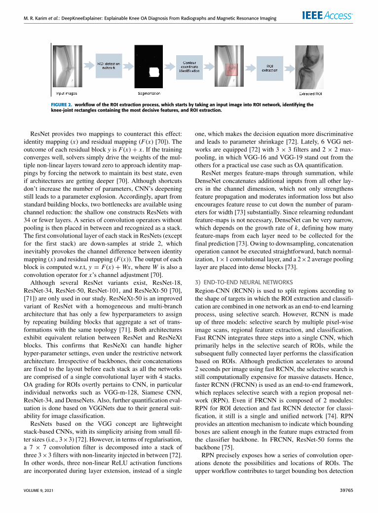
FIGURE 2. workflow of the ROI extraction process, which starts by taking an input image into ROI network, identifying theknee-joint rectangles containing the most decisive features, and ROI extraction.
ResNet provides two mappings to counteract this effect:identity mapping (x) and residual mapping (F(x) [70]). Theoutcome of each residual block y is F(x) + x. If the trainingconverges well, solvers simply drive the weights of the mul-tiple non-linear layers toward zero to approach identity map-pings by forcing the network to maintain its best state, evenif architectures are getting deeper [70]. Although shortcutsdon’t increase the number of parameters, CNN’s deepeningstill leads to a parameter explosion. Accordingly, apart fromstandard building blocks, two bottlenecks are available usingchannel reduction: the shallow one constructs ResNets with34 or fewer layers. A series of convolution operators withoutpooling is then placed in between and recognized as a stack.The first convolutional layer of each stack in ResNets (exceptfor the first stack) are down-samples at stride 2, whichinevitably provokes the channel difference between identitymapping (x) and residual mapping (F(x)). The output of eachblock is computed w.r.t, y = F(x) + Wx, where W is also aconvolution operator for x’s channel adjustment [70].
Although several ResNet variants exist, ResNet-18,ResNet-34, ResNet-50, ResNet-101, and ResNeXt-50 [70],[71]) are only used in our study. ResNeXt-50 is an improvedvariant of ResNet with a homogeneous and multi-brancharchitecture that has only a few hyperparameters to assignby repeating building blocks that aggregate a set of trans-formations with the same topology [71]. Both architecturesexhibit equivalent relation between ResNet and ResNeXtblocks. This confirms that ResNeXt can handle higherhyper-parameter settings, even under the restrictive networkarchitecture. Irrespective of backbones, their concatenationsare fixed to the layout before each stack as all the networksare comprised of a single convolutional layer with 4 stacks.OA grading for ROIs overtly pertains to CNN, in particularindividual networks such as VGG-m-128, Siamese CNN,ResNet-34, and DenseNets. Also, further quantification eval-uation is done based on VGGNets due to their general suit-ability for image classification.
ResNets based on the VGG concept are lightweightstack-based CNNs, with its simplicity arising from small fil-ter sizes (i.e., 3×3) [72]. However, in terms of regularisation,a 7 × 7 convolution filter is decomposed into a stack ofthree 3×3 filters with non-linearity injected in between [72].In other words, three non-linear ReLU activation functionsare incorporated during layer extension, instead of a single
one, which makes the decision equation more discriminativeand leads to parameter shrinkage [72]. Lately, 6 VGG net-works are equipped [72] with 3 × 3 filters and 2 × 2 max-pooling, in which VGG-16 and VGG-19 stand out from theothers for a practical use case such as OA quantification.
ResNet merges feature-maps through summation, whileDenseNet concatenates additional inputs from all other lay-ers in the channel dimension, which not only strengthensfeature propagation and moderates information loss but alsoencourages feature reuse to cut down the number of param-eters for width [73] substantially. Since relearning redundantfeature-maps is not necessary, DenseNet can be very narrow,which depends on the growth rate of k , defining how manyfeature-maps from each layer need to be collected for thefinal prediction [73]. Owing to downsampling, concatenationoperation cannot be executed straightforward, batch normal-ization, 1×1 convolutional layer, and a 2×2 average poolinglayer are placed into dense blocks [73].
3) END-TO-END NEURAL NETWORKSRegion-CNN (RCNN) is used to split regions according tothe shape of targets in which the ROI extraction and classifi-cation are combined in one network as an end-to-end learningprocess, using selective search. However, RCNN is madeup of three models: selective search by multiple pixel-wiseimage scans, regional feature extraction, and classification.Fast RCNN integrates three steps into a single CNN, whichprimarily helps in the selective search of ROIs, while thesubsequent fully connected layer performs the classificationbased on ROIs. Although prediction accelerates to around2 seconds per image using fast RCNN, the selective search isstill computationally expensive for massive datasets. Hence,faster RCNN (FRCNN) is used as an end-to-end framework,which replaces selective search with a region proposal net-work (RPN). Even if FRCNN is composed of 2 modules:RPN for ROI detection and fast RCNN detector for classi-fication, it still is a single and unified network [74]. RPNprovides an attention mechanism to indicate which boundingboxes are salient enough in the feature maps extracted fromthe classifier backbone. In FRCNN, ResNet-50 forms thebackbone [75].
RPN precisely exposes how a series of convolution oper-ations denote the possibilities and locations of ROIs. Theupper workflow contributes to target bounding box detection
VOLUME 9, 2021 39765
M. R. Karim et al.: DeepKneeExplainer: Explainable Knee OA Diagnosis From Radiographs and Magnetic Resonance Imaging
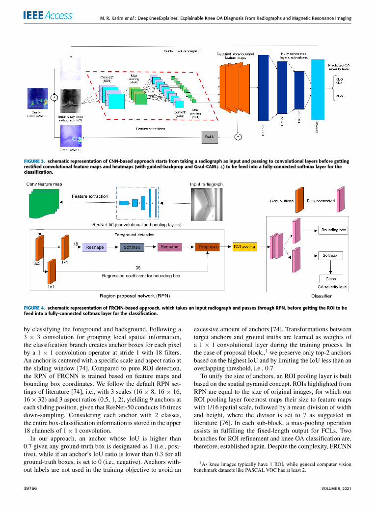
FIGURE 3. schematic representation of CNN-based approach starts from taking a radiograph as input and passing to convolutional layers before gettingrectified convolutional feature maps and heatmaps (with guided-backprop and Grad-CAM++) to be feed into a fully-connected softmax layer for theclassification.
FIGURE 4. schematic representation of FRCNN-based approach, which takes an input radiograph and passes through RPN, before getting the ROI to befeed into a fully-connected softmax layer for the classification.
by classifying the foreground and background. Following a3 × 3 convolution for grouping local spatial information,the classification branch creates anchor boxes for each pixelby a 1 × 1 convolution operator at stride 1 with 18 filters.An anchor is centered with a specific scale and aspect ratio atthe sliding window [74]. Compared to pure ROI detection,the RPN of FRCNN is trained based on feature maps andbounding box coordinates. We follow the default RPN set-tings of literature [74], i.e., with 3 scales (16 × 8, 16 × 16,16× 32) and 3 aspect ratios (0.5, 1, 2), yielding 9 anchors ateach sliding position, given that ResNet-50 conducts 16 timesdown-sampling. Considering each anchor with 2 classes,the entire box-classification information is stored in the upper18 channels of 1× 1 convolution.
In our approach, an anchor whose IoU is higher than0.7 given any ground-truth box is designated as 1 (i.e., posi-tive), while if an anchor’s IoU ratio is lower than 0.3 for allground-truth boxes, is set to 0 (i.e., negative). Anchors with-out labels are not used in the training objective to avoid an
excessive amount of anchors [74]. Transformations betweentarget anchors and ground truths are learned as weights ofa 1 × 1 convolutional layer during the training process. Inthe case of proposal block,,1 we preserve only top-2 anchorsbased on the highest IoU and by limiting the IoU less than anoverlapping threshold, i.e., 0.7.
To unify the size of anchors, an ROI pooling layer is builtbased on the spatial pyramid concept. ROIs highlighted fromRPN are equal to the size of original images, for which ourROI pooling layer foremost maps their size to feature mapswith 1/16 spatial scale, followed by a mean division of widthand height, where the divisor is set to 7 as suggested inliterature [76]. In each sub-block, a max-pooling operationassists in fulfilling the fixed-length output for FCLs. Twobranches for ROI refinement and knee OA classification are,therefore, established again. Despite the complexity, FRCNN
1As knee images typically have 1 ROI, while general computer visionbenchmark datasets like PASCAL VOC has at least 2.
39766 VOLUME 9, 2021
M. R. Karim et al.: DeepKneeExplainer: Explainable Knee OA Diagnosis From Radiographs and Magnetic Resonance Imaging
performs image prediction tasks ten-folds faster than RCNNwhile the whole architecture can be trained synchronouslywithout additional effort.
C. MODEL ENSEMBLESometimes wrong prediction made by the model may leadto the wrong diagnosis, especially when a single practi-tioner makes an OA diagnosis. In such cases, model ensem-bles can help DNNs to achieve improved performance byimplicitly reducing the generalization error. Neural ensem-ble involves training of multiple model snapshots duringa single training run and combine their predictions to anensemble prediction [77], [78]. In the OA diagnosis context,patient risks resulting from one-grade-higher diagnoses aremuch lower than those for one-grade-lower diagnoses. It ismore reasonable to determine the maximum score among thebest standalone model predictions in the ensemble. The bestmodels is selected with WeightWatcher2 [79]. The empiri-cal generalizability study of WeightWatcher shows that thebest trained model tends to show the lowest log-norm andhighest weighted-alpha are only considered. That is, a lowerlog-norm signifies better generalization of network weightsfor unknown test samples [79].
Then, we employ both model fusion and multimodalityintegration to assessing the mean Softmax class posterior andthe maximum among the best performing models regardlessof their architecture type. Inspired by literature [6], [27], [72],[77], averaging their Softmax class posteriors is employed:we pick the best models, ensemble their predictions, andpropagate them through the softmax layer. The class proba-bility of the KL or JSN grade j for a given image x is inferredas follows [6]:
P(y = j|x) =exp
[∑Mm=1 Pm(y = j|x)
]exp
[∑Kk=1
∑Mm=1 Pm(y = k|x)
] , (13)
where M is the number of models in the ensemble, K isthe number of classes, and Pm(y = j|x) is a normalizedprobability distribution. Each module of our multimodalitybased automatic knee OA quantification comprises a set ofmodels, which would be hammered out based on free empir-ical evaluations in section IV.
D. DECISION VISUALIZATIONTo improve knee OA diagnosis transparency and to overcomethe opaqueness, class-discriminating attention map visualiza-tion techniques such as class activation maps (CAM) [80] isproposed to highlight significant features for a class assign-ment. To localize where the model puts more attention onw.r.t classification, CAM computes the number of weightsof each feature map based on the final convolutional layer.CAM aims to calculate the contribution to prediction yc atlocation (i, j), where the goal is to obtain Lcij that satisfiesyc =
∑i,j L
cij. The last feature map Aijk and the prediction
2https://github.com/CalculatedContent/WeightWatcher
yc are represented in a linear relationship in which linearlayers consist of global average pooling (GAP) and FCL: i)GAP outputs Fk =
∑i,j Aijk , ii) FCL that holds weight wck ,
generates the following output [81]:
yc =∑k
wckFk =∑k
wck∑i,j
Aijk =∑i,j
∑k
wckAijk , (14)
where Lcij =∑
k wckAijk [81]. Finally, heat maps (HM) are
plotted to visualize the weighted combination of the fea-ture maps. However, if linear layers replace the classifierarchitecture, re-training of the network is required, and thenon-linearity of the classifier vanishes. Literature [82] cameup with an efficient generalization of CAM called Grad-CAM, where instead of pooling, it globally averages gradi-ents of feature maps as weights.
The guided backpropagation in Grad-CAM can generatemore human-interpretable, but fewer class-sensitive visu-alizations than saliency maps (SM) [83]. Since SM usetrue gradients, trained weights impose substantial biasestowards specific subsets of the input pixels, making theclass-relevant pixels are highlighted instead of producingrandom noise [83]. Therefore, Grad-CAM is used to drawHM to provide attention to discriminating regions, while theclass-specific weights of eachHM are collected from the finalconvolutional layer via globally averaged gradients (GAG) ofFM instead of pooling [84]:
αck =1Z
∑i
∑j
∂yc
∂Akij, (15)
where Z is the number of pixels in an FM, c is the gradient ofthe class, and Akij is the value of k th FM. Based on relativeweights, the coarse SM, Lc is computed as the weightedsum of αck ∗ A
kij of the ReLU activation function. Moreover,
it introduces linear combination to the FM, since only thefeatures with a positive influence on the respective class areof interest [84] and the negative pixels that belong to othercategories in the image are discarded [82]:
Lc = ReLU(∑i
αckAk ). (16)
However, if an image contains multiple objects withslightly different orientations or views of the same class,several objects would fade away in the saliency map createdby Grad-CAM. Moreover, merely parts of objects are spot-lighted by Grad-CAM, as it overlooks significant disparityamong pixels. To improve this bottleneck, Grad-CAM++is proposed [84], which replaces the GAG with a weightedaverage pixel-wise gradients3 via subsequent iterators overthe same activation map Ak , (i, j) and (a, b) [82]:
wck =∑i
∑j
αkcij · ReLU(∂yc
∂Akij) (17)
3As the weights of pixels contribute to the final prediction
VOLUME 9, 2021 39767
M. R. Karim et al.: DeepKneeExplainer: Explainable Knee OA Diagnosis From Radiographs and Magnetic Resonance Imaging
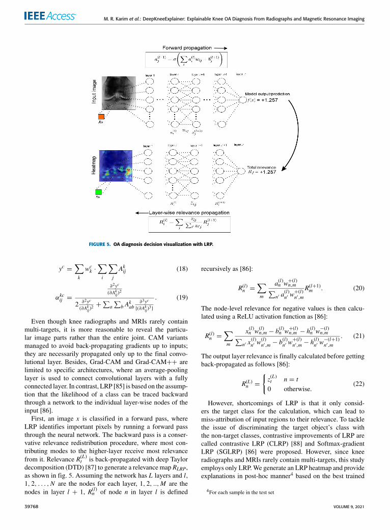
FIGURE 5. OA diagnosis decision visualization with LRP.
yc =∑k
wck ·∑i
∑j
Akij (18)
αkcij =
∂2yc
(∂Akij)2
2 ∂2yc
(∂Akij)2 +
∑a∑
b Akab
∂3yc
{(∂Akij)3}
. (19)
Even though knee radiographs and MRIs rarely containmulti-targets, it is more reasonable to reveal the particu-lar image parts rather than the entire joint. CAM variantsmanaged to avoid back-propagating gradients up to inputs;they are necessarily propagated only up to the final convo-lutional layer. Besides, Grad-CAM and Grad-CAM++ arelimited to specific architectures, where an average-poolinglayer is used to connect convolutional layers with a fullyconnected layer. In contrast, LRP [85] is based on the assump-tion that the likelihood of a class can be traced backwardthrough a network to the individual layer-wise nodes of theinput [86].
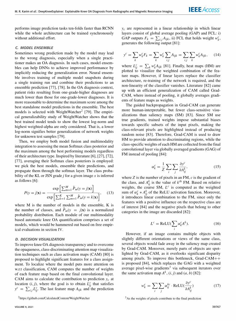
First, an image x is classified in a forward pass, whereLRP identifies important pixels by running a forward passthrough the neural network. The backward pass is a conser-vative relevance redistribution procedure, where most con-tributing modes to the higher-layer receive most relevancefrom it. Relevance R(L)t is back-propagated with deep Taylordecomposition (DTD) [87] to generate a relevance map RLRP,as shown in fig. 5. Assuming the network has L layers and l,1, 2, . . . ,N are the nodes for each layer, 1, 2, ..,M are thenodes in layer l + 1, R(l)n of node n in layer l is defined
recursively as [86]:
R(l)n =∑m
a(l)n w+(l)n,m∑
n′ a(l)n′ w+(l)n′,m
R(l+1)m . (20)
The node-level relevance for negative values is then calcu-lated using a ReLU activation function as [86]:
R(l)n =∑m
x(l)n w(l)n,m − b
(l)n w+(l)n,m − h
(l)n w−(l)n,m∑
n′ x(l)n′ w
(l)n′,m − b
(l)n′ w+(l)n′,m − h
(l)n′ w−(l+1)n′,m
. (21)
The output layer relevance is finally calculated before gettingback-propagated as follows [86]:
R(L)n =
{z(L)t n = t0 otherwise.
(22)
However, shortcomings of LRP is that it only consid-ers the target class for the calculation, which can lead tomiss-attribution of input regions to their relevance. To tacklethe issue of discriminating the target object’s class withthe non-target classes, contrastive improvements of LRP arecalled contrastive LRP (CLRP) [88] and Softmax-gradientLRP (SGLRP) [86] were proposed. However, since kneeradiographs and MRIs rarely contain multi-targets, this studyemploys only LRP.We generate an LRP heatmap and provideexplanations in post-hoc manner4 based on the best trained
4For each sample in the test set
39768 VOLUME 9, 2021
M. R. Karim et al.: DeepKneeExplainer: Explainable Knee OA Diagnosis From Radiographs and Magnetic Resonance Imaging
CNN model,5 where each heatmap indicates the voxel-wiserelevance for the particular classification decision.
IV. EXPERIMENT RESULTSIn this section, we discuss the evaluation results both quanti-tatively and qualitatively, followed by a comparative analysiswith state-of-the-art approaches.
A. EXPERIMENT SETUPAll the programs6 were implemented in Keras andscikit-learn with the TensorFlow backend. Networks weretrained on an Nvidia Titan Xp GPU. Results based on besthyperparameters produced through random search and 5-foldcross-validation are reported empirically.7 We do not ini-tialize network weights with any ImageNet like pretrainedmodels, as they often contain photos of general objects, whichwould activate the internal representation of the network’shidden layers with geometrical forms, colorful patterns,or irrelevant shapes that are usually not present in CXRimages. However, during model inferencing, the test sampleswere preprocessed by passing through the same deep-stackedtransformation pipeline for domain generalization, where theprobability to apply each transformation is set to 0.5. Apartfrom vertex coordinate distances, Adam optimizer is used tooptimize the BCE on the extracted ROIs.
Further, effects of adding Gaussian noise layers8 toimprove model generalization towards unseen test data.Gaussian noise is a natural choice as a corruption processfor real-valued inputs, which makes it suitable to introducenoise to input values or between hidden layers. Althoughaccuracy is an intuitive evaluation criterion for OA severitygrading [89], we report macro-averaged precision, recall,and F1 in the multiclass setting, with widely different classdistributions between different scoring systems, perspectives,and modalities.
B. DATASETRadiographs, 2D MRI slices, and ground truths covering3,026 subjects and their six follow-up examinations arecollected9 from the MOST study [90]. Out of 3,026 kneeradiographic assessments, only 2,406 mutual patients wereengaged in the MRI collection. To mitigate possible decisionbias and out-of-distributions, we do not consider datasets likeThe Osteoarthritis Initiative (OAI).10 However, to maintaindata integrity, this study and the subsequent evaluation arebased on the first visit data (V0) that providesMRI slices from4 perspectives: 4,812 radiographs from the coronal plane,4,748 radiographs from the sagittal plane, 4,676 MRI slicesfrom the axial plane, and 4,678 MRI slices.
5The best model, which we use for the decision visualizations is chosenusing WeightWatcher [79].
6https://github.com/rezacsedu/DeepKneeOAExplainer_7Trained models will be made publicly available8Between the 1st & the 2nd convolution layer for each classifier9http://most.ucsf.edu/10https://oai.epi-ucsf.org/datarelease/
MOST provides 3 types of semi-quantitative scoring sys-tems: KL scale, OARSI JSN progression gauged from themedial tibiofemoral compartment, and OARSI JSN progres-sion assessed from the lateral tibiofemoral compartment.Considering the prevalence of KL in automatic MRI quan-tification and multimodality integration, we assign the sameradiographic semi-quantitative labels for both radiographsandMRIs. However, JSN progressions of lateral tibiofemoralcompartments are excessively imbalanced, and hence onlythe first two grading schemes were adopted.
C. ANALYSIS OF ROI DETECTIONAccurate detection of ROIs highly depends on available seg-mentation ground truths. Therefore, knee joints are manu-ally annotated, regardless of the size as the shapes of kneejoints from the sagittal plane is altered flexibly. According tobounding boxes specification, ground truths of X-ray imagesare converted to binary images with the same sizes as inputimages. FCN and U-Net are thoroughly trained, which helpedto improve previous segmentation loss functions from singleBCE or IoU loss to their standard sum. The combination ofBCE loss and accuracy only measures which percentage ofinput images has a higher IoU score>55%. The recorded IoUlosses and IoU scores, which are void of the pixel-wise plane,are presented in table 4.
The mean IoU of our approach (i.e., 0.846 on MOSTcohort) is quite in line with the baseline (0.81 using FCN-32s on the MOST cohort [32]). It confirms the rationalityand comparability of our evaluation. Further, upgrading fromFCN-32s to FCN-8s improves the IoU score, and the increaseof around 0.01 for X-ray images acquired from both planes isfar away from expectation. Compared to IoUs resulting fromU-Net segmentation, which improves the score by at least 0.1,expose the critical shortcomings of the FCN architecture. Theconcatenation for each pooling layer impeccably preservesall local features, while vast spatial information is still lostduring downsampling and summation. ResNet-18 performsconsistently well, regardless of the X-ray plane and evalua-tion criteria, as outlined in table 5. Norman et al. [27] reporta 98.3% accuracy for ResNet-18, based on the detection rateof coronal radiographs with IoU>0.5. In contrast, we experi-enced an ROI detection rate for IoU>0.55 and IoU>0.77 of100% and a mean IoU of 0.98, for U-Net architecture withthe ResNet-18 backbone.
As knee joints from the coronal plane are moremonotonous than those from the sagittal plane, the averageIoUs of sagittal X-ray images are lower or equal to 4%. How-ever, aiming at 2-class bounding box detection - a relativelysimple segmentation task, U-Net with more complicatedstructures are prone to overfitting. This is reflected by amildly decreasing trend of IoU scores, as reported in table 4.The overfitting issue explains why backbones with morelayers suit smaller batch sizes better and might be preferablefor ROI detection on sagittal radiographs. Overall, U-Netswith complex backbones are found to be more suitable for
VOLUME 9, 2021 39769
M. R. Karim et al.: DeepKneeExplainer: Explainable Knee OA Diagnosis From Radiographs and Magnetic Resonance Imaging
TABLE 4. ROI detection results on radiographs (coronal+sagittal planes).
TABLE 5. IoUs of RPNs vs. pure ROI detection approaches.
accurate segmentation tasks. Hence, we picked U-Net basedon ResNet-18 for ROI detection over CNN.
The comparison between IoUs of RPNs and pure ROIdetection is depicted in table 5. As shown, the more accu-rate radiographs are classified, the more likely RPNs arefostered to attain similar or even better IoU scores thanthe U-Net, which holds for coronal radiographs. However,RPN’s performance is slightly limited by its grading diffi-culty for sagittal radiographs. Although RPN’s architecturesimplicity is an advantage as it merges two model trainingand skips the ROI extraction step by taking a macroscopicview, it ignores ground truths from detail implementationand directly replaces them by bounding box coordinates,which leaves no room for contour detection. Consequently,the predicted bounding boxes from RPNs are extracted rightaway for all the following experiments. Even though RPN’sIoU average for sagittal X-ray images is slightly lower thanthat of U-Net with ResNet-18 backbone, it can still take upthe second rank with superior performance.
D. PERFORMANCE OF INDIVIDUAL MODELSWe provide a detailed analysis of individual models beforeselecting the best ones for the ensemble.
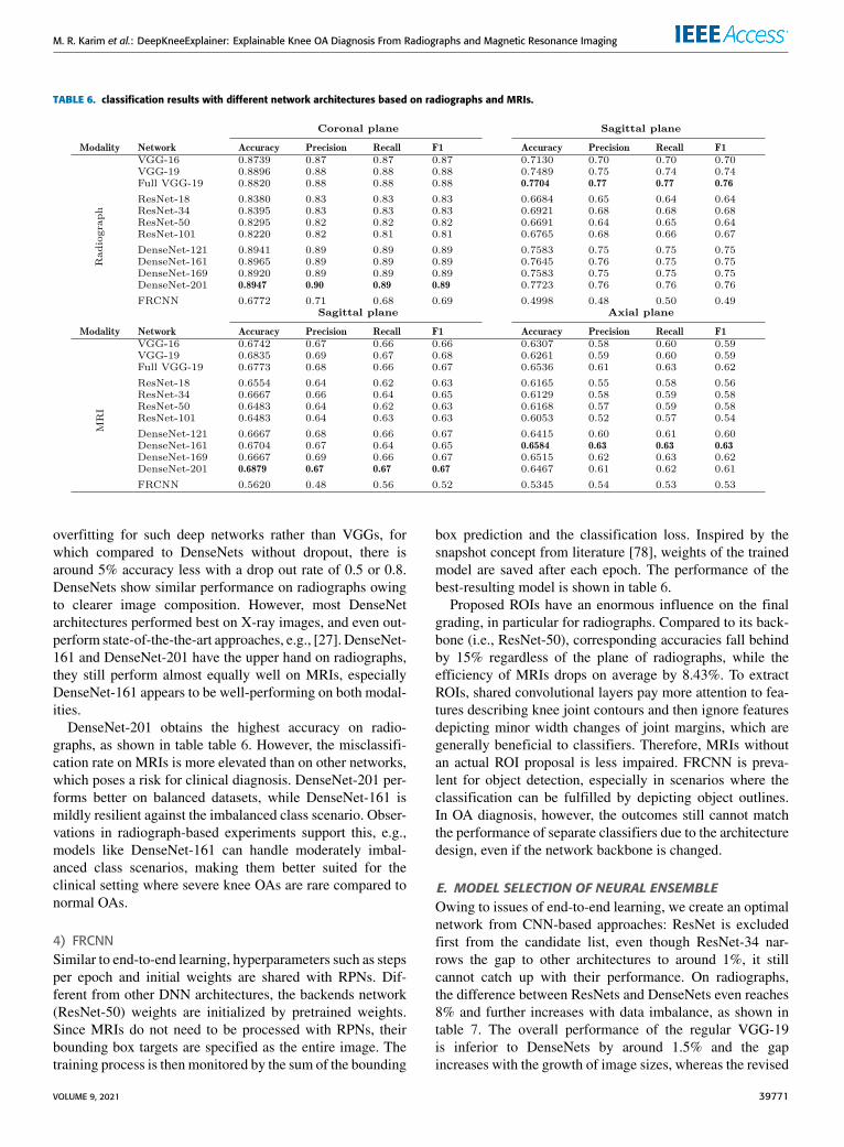
1) VGG ARCHITECTURESAlthough VGG-16 enlarges octuple and quadruple numbersof hidden nodes for each layer, the diagnosis from VGG-19 ismore reliable overall, as shown in table 6. The superiorityis more significant for sagittal knee joints since classifierswith more formations require more fitting of feature maps,which again relies on convolutional layers. The extractionof JSN-related features from the axial MRI plane is morechallenging which leads to a similar performance. The archi-tecturemodification in VGG-19 by setting the number of con-volutional layers to 2 with a filter size of 16, visibly enhancesthe performance of VGG-19 on sagittal radiographs andaxial MRIs as shown in table 6. Moreover, when using bal-anced datasets, macro average precision, recall, and F1 were
improved, given that the training is less biased towards certainclass predictions.
2) ResNetsPre-trained ResNets are not used for the weight initialization;rather, each ResNet was trained from scratch with validationaccuracy monitoring. The results are summarized in table 6.Eventually, ResNet-34 performed the best. However, on themost monotonous dataset - the coronal plane radiographs -smaller networks like the ResNet-18 show an almost similarperformance. For the sagittal plane, ResNet-101 tops sec-ond since shapes of knee joints from the sagittal plane verystrongly. Similar to VGGs, ResNet-18 and ResNet-50 per-form quite similar on axial MRIs. Evidently, due to thestructured residual blocks, the accumulation of layers cannotpromote feature maps extracted from the axial view. Short-cuts may even only connect it, making the axial view is notinformative for JSN scoring.
3) DenseNetsCompared to ResNets, DenseNets improve validation accu-racies quite slowly during training. This is mainly due tomultiple connections within dense blocks, albeit batch sizedoes not have a decisive impact on the performance. Thiscan be accounted for by using more training epochs. Acrossexperiments, the accuracy difference stays roughly within arange of 2%. InDenseNets we keep the growth rate at 12 sinceprevious research found superior performance for image clas-sification tasks [73] using a narrow structure with 12 channelgrowth per layer. Inspired by the method for searching idealfilter numbers in VGG convolutional layers, we set 4, 8,12, and 16 as the initial filter size in which 8 appears tobe optimal, giving the highest accuracy and speed. Filternumbers are set small enough to leave the reduction rateunchanged from the default hyperparameter setting (i.e., 0.5)and preserved the dropout rate at 0.
Besides, since MOST images are supplied in DICOMformat, even though each group of medical images isexpanded by data augmentation, it is still far away from
39770 VOLUME 9, 2021
M. R. Karim et al.: DeepKneeExplainer: Explainable Knee OA Diagnosis From Radiographs and Magnetic Resonance Imaging
TABLE 6. classification results with different network architectures based on radiographs and MRIs.
overfitting for such deep networks rather than VGGs, forwhich compared to DenseNets without dropout, there isaround 5% accuracy less with a drop out rate of 0.5 or 0.8.DenseNets show similar performance on radiographs owingto clearer image composition. However, most DenseNetarchitectures performed best on X-ray images, and even out-perform state-of-the-the-art approaches, e.g., [27]. DenseNet-161 and DenseNet-201 have the upper hand on radiographs,they still perform almost equally well on MRIs, especiallyDenseNet-161 appears to be well-performing on both modal-ities.
DenseNet-201 obtains the highest accuracy on radio-graphs, as shown in table table 6. However, the misclassifi-cation rate on MRIs is more elevated than on other networks,which poses a risk for clinical diagnosis. DenseNet-201 per-forms better on balanced datasets, while DenseNet-161 ismildly resilient against the imbalanced class scenario. Obser-vations in radiograph-based experiments support this, e.g.,models like DenseNet-161 can handle moderately imbal-anced class scenarios, making them better suited for theclinical setting where severe knee OAs are rare compared tonormal OAs.
4) FRCNNSimilar to end-to-end learning, hyperparameters such as stepsper epoch and initial weights are shared with RPNs. Dif-ferent from other DNN architectures, the backends network(ResNet-50) weights are initialized by pretrained weights.Since MRIs do not need to be processed with RPNs, theirbounding box targets are specified as the entire image. Thetraining process is then monitored by the sum of the bounding
box prediction and the classification loss. Inspired by thesnapshot concept from literature [78], weights of the trainedmodel are saved after each epoch. The performance of thebest-resulting model is shown in table 6.
Proposed ROIs have an enormous influence on the finalgrading, in particular for radiographs. Compared to its back-bone (i.e., ResNet-50), corresponding accuracies fall behindby 15% regardless of the plane of radiographs, while theefficiency of MRIs drops on average by 8.43%. To extractROIs, shared convolutional layers pay more attention to fea-tures describing knee joint contours and then ignore featuresdepicting minor width changes of joint margins, which aregenerally beneficial to classifiers. Therefore, MRIs withoutan actual ROI proposal is less impaired. FRCNN is preva-lent for object detection, especially in scenarios where theclassification can be fulfilled by depicting object outlines.In OA diagnosis, however, the outcomes still cannot matchthe performance of separate classifiers due to the architecturedesign, even if the network backbone is changed.
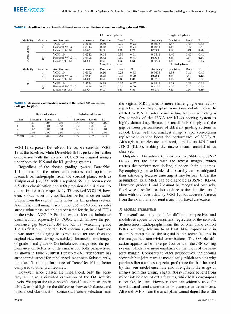
E. MODEL SELECTION OF NEURAL ENSEMBLEOwing to issues of end-to-end learning, we create an optimalnetwork from CNN-based approaches: ResNet is excludedfirst from the candidate list, even though ResNet-34 nar-rows the gap to other architectures to around 1%, it stillcannot catch up with their performance. On radiographs,the difference between ResNets and DenseNets even reaches8% and further increases with data imbalance, as shown intable 7. The overall performance of the regular VGG-19is inferior to DenseNets by around 1.5% and the gapincreases with the growth of image sizes, whereas the revised
VOLUME 9, 2021 39771
M. R. Karim et al.: DeepKneeExplainer: Explainable Knee OA Diagnosis From Radiographs and Magnetic Resonance Imaging
TABLE 7. classification results with different network architectures based on radiographs and MRIs.
TABLE 8. classwise classification results of DenseNet-161 on coronalradiographs (JSN).
VGG-19 surpasses DenseNets. Hence, we consider VGG-19 as the baseline, while DenseNet-161 is picked for furthercomparison with the revised VGG-19 on original imagesunder both the JSN and the KL grading systems.
Regardless of the chosen grading system, DenseNet-161 dominates the other architectures and up-to-dateresearch on radiographs from the coronal plane, such asTiulpin et al. [6], [37] with a reported 66.71% accuracy ona 5-class classification and 0.68 precision on a 4-class OAquantification task, respectively. The revised VGG-19, how-ever, shows superior classification performance on radio-graphs from the sagittal plane under the KL grading system.Assuming a full image resolution of 355× 568 pixels renderstrong robustness, which compensated for the lack of FCLsin the revised VGG-19. Further, we consider the imbalanceclassification, especially for VGGs, which narrows the per-formance gap between JSN and KL by weakening grade1 classification under the JSN scoring system. However,it was more challenging to extract exact features from thesagittal view considering the subtle difference is some imagesof grade 1 and grade 0. On imbalanced image sets, the per-formance on MRIs is quite similar for both perspectives,as shown in table 7, albeit DenseNet-161 architecture hasstronger robustness for imbalanced image sets. Subsequently,the classification performance of DenseNet-161 is bettercompared to other architectures.
However, since classes are imbalanced, only the accu-racy will give a distorted estimation of the OA severitylevels. We report the class-specific classification measures intable 8, to shed light on the differences between balanced andimbalanced classification scenarios. Feature selection from
the sagittal MRI planes is more challenging even involv-ing KL-2 since they display more knee details indirectlyrelated to JSN. Besides, constructing features reflecting afew samples of the JSN-3 (or KL-4) scoring system ishighly demanding. Hence, the recall falls sharply and thegap between performances of different grading systems issealed. Even with the smallest image shape, convolutionreplacement cannot boost the performance of VGG-19.Although accuracies are enhanced, it relies on JSN-0 andJSN-2 (KL-3), making the macro means unsatisfied asobserved.
Outputs of DenseNet-161 also tend to JSN-0 and JSN-2(KL-3), but the class with the fewest images, whichretards the performance decline, supports their outcomes.By employing dense blocks, data scarcity can be mitigatedthan extracting features directing at tiny lesions. Under theassumption, axial MRIs can be diagnosed as JSN-3 (KL-4).However, grades 1 and 2 cannot be recognized precisely.Pixel-wise classification also conduces to the identification ofclass with the fewest data by VGG-19, but accurate featuresfrom the axial plane for joint margin portrayal are scarce.
F. MODEL ENSEMBLEThe overall accuracy trend for different perspectives andmodalities appear to be consistent, regardless of the networkarchitectures. Radiographs from the coronal plane exhibitbetter accuracy, leading to at least 14% improvement inaccuracy compared to the sagittal plane: fewer features inthe images had non-trivial contributions. The OA classifi-cation appears to be more productive with the JSN scoringsystem, which lays more emphasis on the width of the kneejoint margin. Compared to other perspectives, the coronalview exhibits joint margins most clearly, which explains whyprevious literature has a special preference for that. Inspiredby this, our model ensemble also strengthens the usage ofimages from this group. Sagittal X-ray images benefit fromminor interference of extra features, while MRIs encompassricher OA features. However, they are seldomly used forsophisticated semi-quantitative or quantitative assessments.Although MRIs from the axial plane cannot depict the width
39772 VOLUME 9, 2021
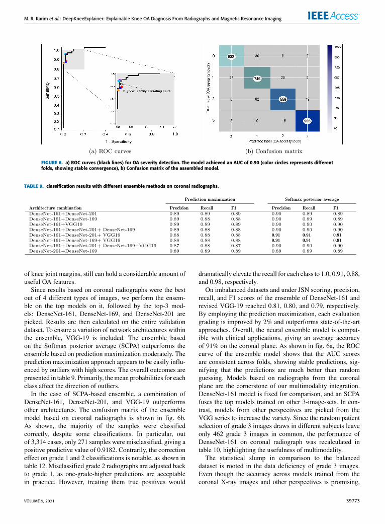
M. R. Karim et al.: DeepKneeExplainer: Explainable Knee OA Diagnosis From Radiographs and Magnetic Resonance Imaging
FIGURE 6. a) ROC curves (black lines) for OA severity detection. The model achieved an AUC of 0.90 (color circles represents differentfolds, showing stable convergence), b) Confusion matrix of the assembled model.
TABLE 9. classification results with different ensemble methods on coronal radiographs.
of knee joint margins, still can hold a considerable amount ofuseful OA features.
Since results based on coronal radiographs were the bestout of 4 different types of images, we perform the ensem-ble on the top models on it, followed by the top-3 mod-els: DenseNet-161, DenseNet-169, and DenseNet-201 arepicked. Results are then calculated on the entire validationdataset. To ensure a variation of network architectures withinthe ensemble, VGG-19 is included. The ensemble basedon the Softmax posterior average (SCPA) outperforms theensemble based on prediction maximization moderately. Theprediction maximization approach appears to be easily influ-enced by outliers with high scores. The overall outcomes arepresented in table 9. Primarily, themean probabilities for eachclass affect the direction of outliers.
In the case of SCPA-based ensemble, a combination ofDenseNet-161, DenseNet-201, and VGG-19 outperformsother architectures. The confusion matrix of the ensemblemodel based on coronal radiographs is shown in fig. 6b.As shown, the majority of the samples were classifiedcorrectly, despite some classifications. In particular, outof 3,314 cases, only 271 samples were misclassified, giving apositive predictive value of 0.9182. Contrarily, the correctioneffect on grade 1 and 2 classifications is notable, as shown intable 12. Misclassified grade 2 radiographs are adjusted backto grade 1, as one-grade-higher predictions are acceptablein practice. However, treating them true positives would
dramatically elevate the recall for each class to 1.0, 0.91, 0.88,and 0.98, respectively.
On imbalanced datasets and under JSN scoring, precision,recall, and F1 scores of the ensemble of DenseNet-161 andrevised VGG-19 reached 0.81, 0.80, and 0.79, respectively.By employing the prediction maximization, each evaluationgrading is improved by 2% and outperforms state-of-the-artapproaches. Overall, the neural ensemble model is compat-ible with clinical applications, giving an average accuracyof 91% on the coronal plane. As shown in fig. 6a, the ROCcurve of the ensemble model shows that the AUC scoresare consistent across folds, showing stable predictions, sig-nifying that the predictions are much better than randomguessing. Models based on radiographs from the coronalplane are the cornerstone of our multimodality integration.DenseNet-161 model is fixed for comparison, and an SCPAfuses the top models trained on other 3-image-sets. In con-trast, models from other perspectives are picked from theVGG series to increase the variety. Since the random patientselection of grade 3 images draws in different subjects leaveonly 462 grade 3 images in common, the performance ofDenseNet-161 on coronal radiograph was recalculated intable 10, highlighting the usefulness of multimodality.
The statistical slump in comparison to the balanceddataset is rooted in the data deficiency of grade 3 images.Even though the accuracy across models trained from thecoronal X-ray images and other perspectives is promising,
VOLUME 9, 2021 39773
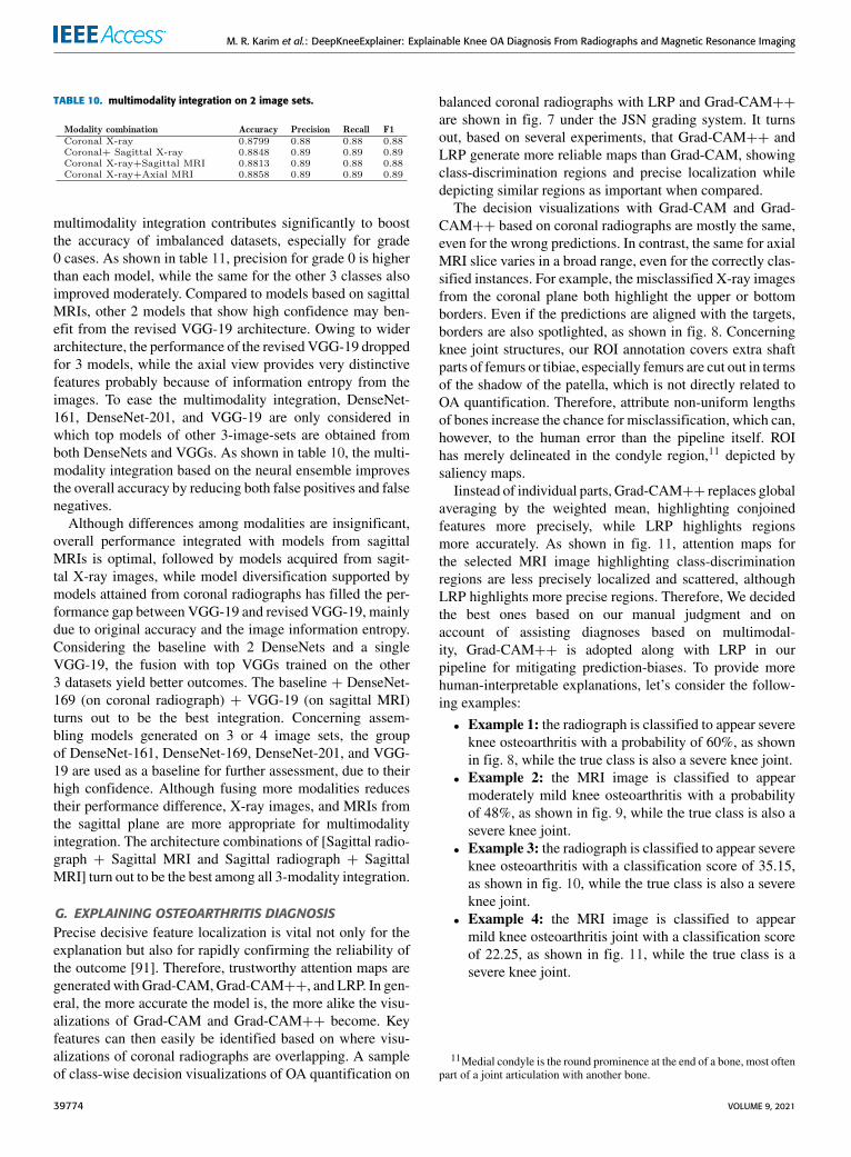
M. R. Karim et al.: DeepKneeExplainer: Explainable Knee OA Diagnosis From Radiographs and Magnetic Resonance Imaging
TABLE 10. multimodality integration on 2 image sets.
multimodality integration contributes significantly to boostthe accuracy of imbalanced datasets, especially for grade0 cases. As shown in table 11, precision for grade 0 is higherthan each model, while the same for the other 3 classes alsoimproved moderately. Compared to models based on sagittalMRIs, other 2 models that show high confidence may ben-efit from the revised VGG-19 architecture. Owing to widerarchitecture, the performance of the revised VGG-19 droppedfor 3 models, while the axial view provides very distinctivefeatures probably because of information entropy from theimages. To ease the multimodality integration, DenseNet-161, DenseNet-201, and VGG-19 are only considered inwhich top models of other 3-image-sets are obtained fromboth DenseNets and VGGs. As shown in table 10, the multi-modality integration based on the neural ensemble improvesthe overall accuracy by reducing both false positives and falsenegatives.
Although differences among modalities are insignificant,overall performance integrated with models from sagittalMRIs is optimal, followed by models acquired from sagit-tal X-ray images, while model diversification supported bymodels attained from coronal radiographs has filled the per-formance gap between VGG-19 and revised VGG-19, mainlydue to original accuracy and the image information entropy.Considering the baseline with 2 DenseNets and a singleVGG-19, the fusion with top VGGs trained on the other3 datasets yield better outcomes. The baseline + DenseNet-169 (on coronal radiograph) + VGG-19 (on sagittal MRI)turns out to be the best integration. Concerning assem-bling models generated on 3 or 4 image sets, the groupof DenseNet-161, DenseNet-169, DenseNet-201, and VGG-19 are used as a baseline for further assessment, due to theirhigh confidence. Although fusing more modalities reducestheir performance difference, X-ray images, and MRIs fromthe sagittal plane are more appropriate for multimodalityintegration. The architecture combinations of [Sagittal radio-graph + Sagittal MRI and Sagittal radiograph + SagittalMRI] turn out to be the best among all 3-modality integration.
G. EXPLAINING OSTEOARTHRITIS DIAGNOSISPrecise decisive feature localization is vital not only for theexplanation but also for rapidly confirming the reliability ofthe outcome [91]. Therefore, trustworthy attention maps aregenerated with Grad-CAM,Grad-CAM++, and LRP. In gen-eral, the more accurate the model is, the more alike the visu-alizations of Grad-CAM and Grad-CAM++ become. Keyfeatures can then easily be identified based on where visu-alizations of coronal radiographs are overlapping. A sampleof class-wise decision visualizations of OA quantification on
balanced coronal radiographs with LRP and Grad-CAM++are shown in fig. 7 under the JSN grading system. It turnsout, based on several experiments, that Grad-CAM++ andLRP generate more reliable maps than Grad-CAM, showingclass-discrimination regions and precise localization whiledepicting similar regions as important when compared.
The decision visualizations with Grad-CAM and Grad-CAM++ based on coronal radiographs are mostly the same,even for the wrong predictions. In contrast, the same for axialMRI slice varies in a broad range, even for the correctly clas-sified instances. For example, the misclassified X-ray imagesfrom the coronal plane both highlight the upper or bottomborders. Even if the predictions are aligned with the targets,borders are also spotlighted, as shown in fig. 8. Concerningknee joint structures, our ROI annotation covers extra shaftparts of femurs or tibiae, especially femurs are cut out in termsof the shadow of the patella, which is not directly related toOA quantification. Therefore, attribute non-uniform lengthsof bones increase the chance for misclassification, which can,however, to the human error than the pipeline itself. ROIhas merely delineated in the condyle region,11 depicted bysaliency maps.
Iinstead of individual parts, Grad-CAM++ replaces globalaveraging by the weighted mean, highlighting conjoinedfeatures more precisely, while LRP highlights regionsmore accurately. As shown in fig. 11, attention maps forthe selected MRI image highlighting class-discriminationregions are less precisely localized and scattered, althoughLRP highlights more precise regions. Therefore, We decidedthe best ones based on our manual judgment and onaccount of assisting diagnoses based on multimodal-ity, Grad-CAM++ is adopted along with LRP in ourpipeline for mitigating prediction-biases. To provide morehuman-interpretable explanations, let’s consider the follow-ing examples:
• Example 1: the radiograph is classified to appear severeknee osteoarthritis with a probability of 60%, as shownin fig. 8, while the true class is also a severe knee joint.
• Example 2: the MRI image is classified to appearmoderately mild knee osteoarthritis with a probabilityof 48%, as shown in fig. 9, while the true class is also asevere knee joint.
• Example 3: the radiograph is classified to appear severeknee osteoarthritis with a classification score of 35.15,as shown in fig. 10, while the true class is also a severeknee joint.
• Example 4: the MRI image is classified to appearmild knee osteoarthritis joint with a classification scoreof 22.25, as shown in fig. 11, while the true class is asevere knee joint.
11Medial condyle is the round prominence at the end of a bone, most oftenpart of a joint articulation with another bone.
39774 VOLUME 9, 2021
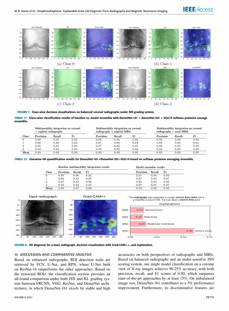
M. R. Karim et al.: DeepKneeExplainer: Explainable Knee OA Diagnosis From Radiographs and Magnetic Resonance Imaging
FIGURE 7. Class-wise decision visualizations on balanced coronal radiographs under JSN grading system.
TABLE 11. Class-wise classification results of baseline vs. model ensemble with DenseNet-161 + DenseNet-201 + VGG19 Softmax posterior averageensemble.
TABLE 12. classwise OA quantification results for DenseNet-161+DenseNet-201+VGG19 based on softmax posterior averaging ensemble.
FIGURE 8. OA diagnosis for a knee radiograph, decision visualization with Grad-CAM++, and explanation.
H. DISCUSSION AND COMPARATIVE ANALYSISBased on enhanced radiographs, ROI detection trails areretrieved by FCN, U-Net, and RPN, where U-Net builton ResNet-18 outperforms the other approaches. Based onthe extracted ROIs, the classification section provides anall-round comparison under both JSN and KL grading sys-tem between FRCNN, VGG, ResNet, and DenseNet archi-tectures, in which DenseNet-161 excels by stable and high
accuracies on both perspectives of radiographs and MRIs.Based on balanced radiographs and an under-sensitive JSNscoring system, our single model classification on a coronalview of X-ray images achieves 90.25% accuracy, with bothprecision, recall, and F1 scores of 0.90, which surpassesstate-of-the-art approaches by at least 15%. On imbalancedimage sets, DenseNet-161 contributes to a 5% performanceimprovement. Furthermore, its discriminative features are
VOLUME 9, 2021 39775
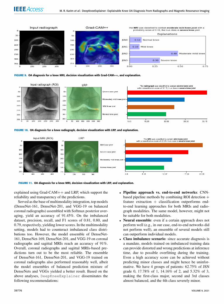
M. R. Karim et al.: DeepKneeExplainer: Explainable Knee OA Diagnosis From Radiographs and Magnetic Resonance Imaging
FIGURE 9. OA diagnosis for a knee MRI, decision visualization with Grad-CAM++, and explanation.
FIGURE 10. OA diagnosis for a knee radiograph, decision visualization with LRP, and explanation.
FIGURE 11. OA diagnosis for a knee MRI, decision visualization with LRP, and explanation.
explained using Grad-CAM++ and LRP, which support thereliability and transparency of the predictions.
Served as the base ofmultimodality integration, topmodels(DenseNet-161, DenseNet-201, and VGG-19 on balancedcoronal radiographs) assembled with Softmax posterior aver-aging, yield an accuracy of 91.45%. On the imbalanceddataset, precision, recall, and F1 scores of 0.81, 0.80, and0.79, respectively, yielding lower scores. In themultimodalitysetting, models had to counteract imbalanced class distri-butions too. However, the model ensemble of DenseNet-161, DenseNet-169, DenseNet-201, and VGG-19 on coronalradiographs and sagittal MRIs reach an accuracy of 91%.Overall, coronal radiographs and sagittal MRIs-based pre-dictions turn out to be the most reliable. The ensembleof DenseNet-161, DenseNet-201, and VGG-19 trained oncoronal radiographs also performed reasonably well, albeitthe model ensembles of balanced prediction mixture ofDenseNets and VGGs yielded a better result. Based on theabove analyses, DeepKneeExplainer disseminates thefollowing recommendations:
• Pipeline approach vs. end-to-end networks: CNN-based pipeline methods by combining ROI detection +feature extraction + classification outperforms end-to-end learning approaches for both MRIs and radio-graph modalities. The same model, however, might notbe suitable for both modalities.
• Neural ensemble: even if a certain approach does notperform well (e.g., in our case, end-to-end networks didnot perform well), an ensemble of several models stillcan outperform individual models.
• Class imbalance scenario: since accurate diagnosis isa mandate, models trained on imbalanced training datacan provide distorted and wrong predictions at inferencetime, due to possible overfitting during the training.Even a high accuracy score can be achieved withoutpredicting minor classes and might hence be uninfor-mative. We have 4 groups of patients: 62.75% of JSNgrade 0, 17.78% of 1, 14.16% of 2, and 5.32% of 3,making the first-class major, second and 3rd classesalmost balanced, and the 4th class severely minor.
39776 VOLUME 9, 2021
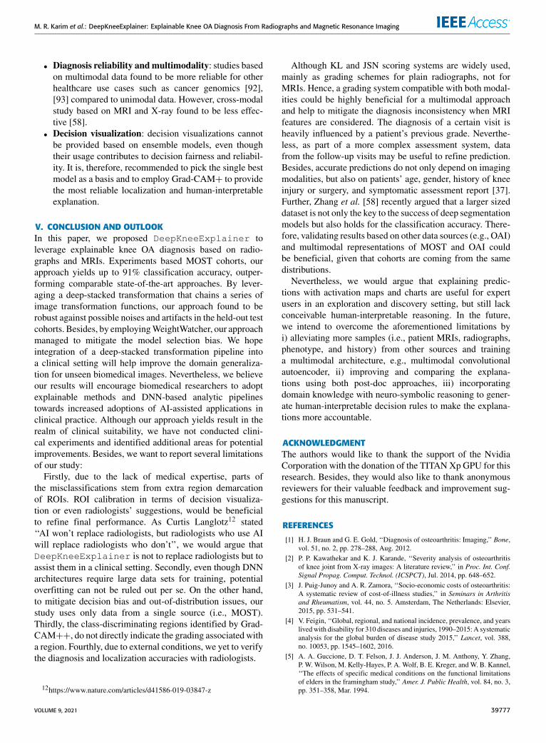
M. R. Karim et al.: DeepKneeExplainer: Explainable Knee OA Diagnosis From Radiographs and Magnetic Resonance Imaging
• Diagnosis reliability andmultimodality: studies basedon multimodal data found to be more reliable for otherhealthcare use cases such as cancer genomics [92],[93] compared to unimodal data. However, cross-modalstudy based on MRI and X-ray found to be less effec-tive [58].
• Decision visualization: decision visualizations cannotbe provided based on ensemble models, even thoughtheir usage contributes to decision fairness and reliabil-ity. It is, therefore, recommended to pick the single bestmodel as a basis and to employ Grad-CAM+ to providethe most reliable localization and human-interpretableexplanation.
V. CONCLUSION AND OUTLOOKIn this paper, we proposed DeepKneeExplainer toleverage explainable knee OA diagnosis based on radio-graphs and MRIs. Experiments based MOST cohorts, ourapproach yields up to 91% classification accuracy, outper-forming comparable state-of-the-art approaches. By lever-aging a deep-stacked transformation that chains a series ofimage transformation functions, our approach found to berobust against possible noises and artifacts in the held-out testcohorts. Besides, by employingWeightWatcher, our approachmanaged to mitigate the model selection bias. We hopeintegration of a deep-stacked transformation pipeline intoa clinical setting will help improve the domain generaliza-tion for unseen biomedical images. Nevertheless, we believeour results will encourage biomedical researchers to adoptexplainable methods and DNN-based analytic pipelinestowards increased adoptions of AI-assisted applications inclinical practice. Although our approach yields result in therealm of clinical suitability, we have not conducted clini-cal experiments and identified additional areas for potentialimprovements. Besides, we want to report several limitationsof our study:
Firstly, due to the lack of medical expertise, parts ofthe misclassifications stem from extra region demarcationof ROIs. ROI calibration in terms of decision visualiza-tion or even radiologists’ suggestions, would be beneficialto refine final performance. As Curtis Langlotz12 stated‘‘AI won’t replace radiologists, but radiologists who use AIwill replace radiologists who don’t’’, we would argue thatDeepKneeExplainer is not to replace radiologists but toassist them in a clinical setting. Secondly, even though DNNarchitectures require large data sets for training, potentialoverfitting can not be ruled out per se. On the other hand,to mitigate decision bias and out-of-distribution issues, ourstudy uses only data from a single source (i.e., MOST).Thirdly, the class-discriminating regions identified by Grad-CAM++, do not directly indicate the grading associated witha region. Fourthly, due to external conditions, we yet to verifythe diagnosis and localization accuracies with radiologists.
12https://www.nature.com/articles/d41586-019-03847-z
Although KL and JSN scoring systems are widely used,mainly as grading schemes for plain radiographs, not forMRIs. Hence, a grading system compatible with both modal-ities could be highly beneficial for a multimodal approachand help to mitigate the diagnosis inconsistency when MRIfeatures are considered. The diagnosis of a certain visit isheavily influenced by a patient’s previous grade. Neverthe-less, as part of a more complex assessment system, datafrom the follow-up visits may be useful to refine prediction.Besides, accurate predictions do not only depend on imagingmodalities, but also on patients’ age, gender, history of kneeinjury or surgery, and symptomatic assessment report [37].Further, Zhang et al. [58] recently argued that a larger sizeddataset is not only the key to the success of deep segmentationmodels but also holds for the classification accuracy. There-fore, validating results based on other data sources (e.g., OAI)and multimodal representations of MOST and OAI couldbe beneficial, given that cohorts are coming from the samedistributions.
Nevertheless, we would argue that explaining predic-tions with activation maps and charts are useful for expertusers in an exploration and discovery setting, but still lackconceivable human-interpretable reasoning. In the future,we intend to overcome the aforementioned limitations byi) alleviating more samples (i.e., patient MRIs, radiographs,phenotype, and history) from other sources and traininga multimodal architecture, e.g., multimodal convolutionalautoencoder, ii) improving and comparing the explana-tions using both post-doc approaches, iii) incorporatingdomain knowledge with neuro-symbolic reasoning to gener-ate human-interpretable decision rules to make the explana-tions more accountable.
ACKNOWLEDGMENTThe authors would like to thank the support of the NvidiaCorporation with the donation of the TITANXp GPU for thisresearch. Besides, they would also like to thank anonymousreviewers for their valuable feedback and improvement sug-gestions for this manuscript.
REFERENCES[1] H. J. Braun and G. E. Gold, ‘‘Diagnosis of osteoarthritis: Imaging,’’ Bone,
vol. 51, no. 2, pp. 278–288, Aug. 2012.[2] P. P. Kawathekar and K. J. Karande, ‘‘Severity analysis of osteoarthritis
of knee joint from X-ray images: A literature review,’’ in Proc. Int. Conf.Signal Propag. Comput. Technol. (ICSPCT), Jul. 2014, pp. 648–652.
[3] J. Puig-Junoy and A. R. Zamora, ‘‘Socio-economic costs of osteoarthritis:A systematic review of cost-of-illness studies,’’ in Seminars in Arthritisand Rheumatism, vol. 44, no. 5. Amsterdam, The Netherlands: Elsevier,2015, pp. 531–541.
[4] V. Feigin, ‘‘Global, regional, and national incidence, prevalence, and yearslivedwith disability for 310 diseases and injuries, 1990–2015: A systematicanalysis for the global burden of disease study 2015,’’ Lancet, vol. 388,no. 10053, pp. 1545–1602, 2016.
[5] A. A. Guccione, D. T. Felson, J. J. Anderson, J. M. Anthony, Y. Zhang,P. W.Wilson, M. Kelly-Hayes, P. A. Wolf, B. E. Kreger, andW. B. Kannel,‘‘The effects of specific medical conditions on the functional limitationsof elders in the framingham study,’’ Amer. J. Public Health, vol. 84, no. 3,pp. 351–358, Mar. 1994.
VOLUME 9, 2021 39777
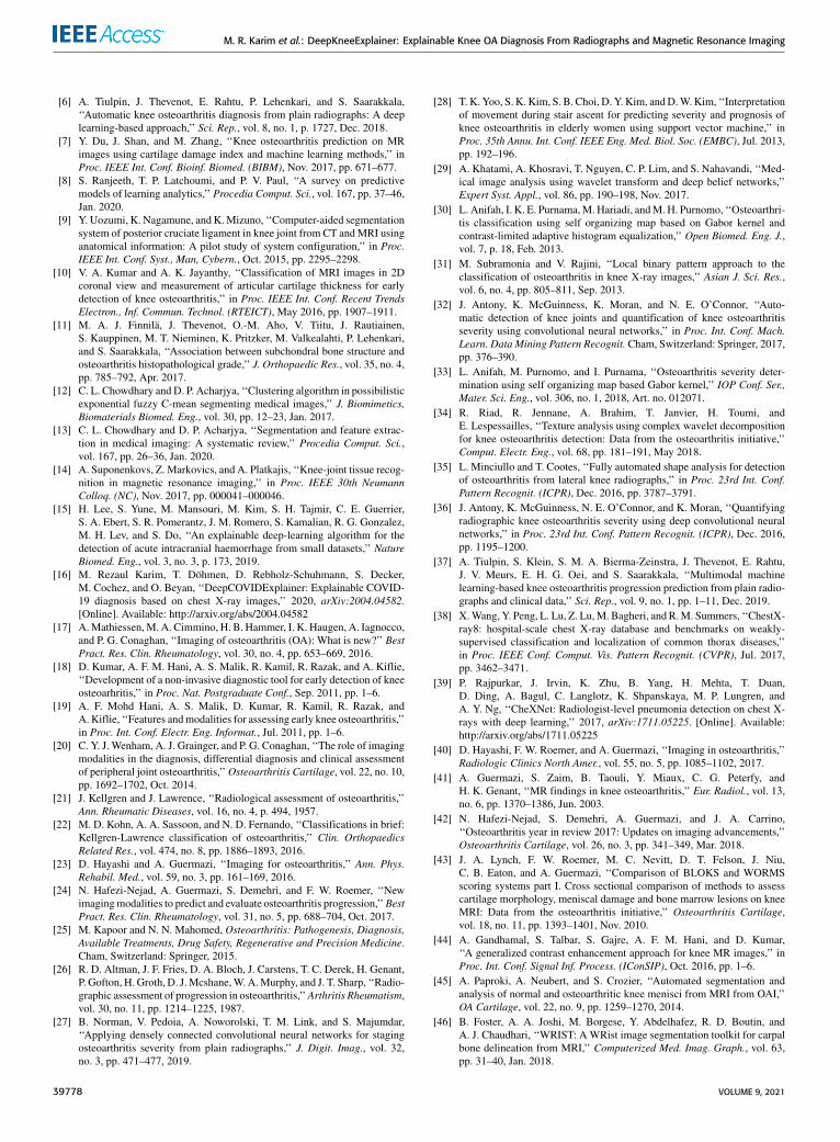
M. R. Karim et al.: DeepKneeExplainer: Explainable Knee OA Diagnosis From Radiographs and Magnetic Resonance Imaging
[6] A. Tiulpin, J. Thevenot, E. Rahtu, P. Lehenkari, and S. Saarakkala,‘‘Automatic knee osteoarthritis diagnosis from plain radiographs: A deeplearning-based approach,’’ Sci. Rep., vol. 8, no. 1, p. 1727, Dec. 2018.
[7] Y. Du, J. Shan, and M. Zhang, ‘‘Knee osteoarthritis prediction on MRimages using cartilage damage index and machine learning methods,’’ inProc. IEEE Int. Conf. Bioinf. Biomed. (BIBM), Nov. 2017, pp. 671–677.
[8] S. Ranjeeth, T. P. Latchoumi, and P. V. Paul, ‘‘A survey on predictivemodels of learning analytics,’’ Procedia Comput. Sci., vol. 167, pp. 37–46,Jan. 2020.
[9] Y. Uozumi, K. Nagamune, and K.Mizuno, ‘‘Computer-aided segmentationsystem of posterior cruciate ligament in knee joint from CT andMRI usinganatomical information: A pilot study of system configuration,’’ in Proc.IEEE Int. Conf. Syst., Man, Cybern., Oct. 2015, pp. 2295–2298.
[10] V. A. Kumar and A. K. Jayanthy, ‘‘Classification of MRI images in 2Dcoronal view and measurement of articular cartilage thickness for earlydetection of knee osteoarthritis,’’ in Proc. IEEE Int. Conf. Recent TrendsElectron., Inf. Commun. Technol. (RTEICT), May 2016, pp. 1907–1911.
[11] M. A. J. Finnilä, J. Thevenot, O.-M. Aho, V. Tiitu, J. Rautiainen,S. Kauppinen, M. T. Nieminen, K. Pritzker, M. Valkealahti, P. Lehenkari,and S. Saarakkala, ‘‘Association between subchondral bone structure andosteoarthritis histopathological grade,’’ J. Orthopaedic Res., vol. 35, no. 4,pp. 785–792, Apr. 2017.
[12] C. L. Chowdhary and D. P. Acharjya, ‘‘Clustering algorithm in possibilisticexponential fuzzy C-mean segmenting medical images,’’ J. Biomimetics,Biomaterials Biomed. Eng., vol. 30, pp. 12–23, Jan. 2017.
[13] C. L. Chowdhary and D. P. Acharjya, ‘‘Segmentation and feature extrac-tion in medical imaging: A systematic review,’’ Procedia Comput. Sci.,vol. 167, pp. 26–36, Jan. 2020.
[14] A. Suponenkovs, Z. Markovics, and A. Platkajis, ‘‘Knee-joint tissue recog-nition in magnetic resonance imaging,’’ in Proc. IEEE 30th NeumannColloq. (NC), Nov. 2017, pp. 000041–000046.
[15] H. Lee, S. Yune, M. Mansouri, M. Kim, S. H. Tajmir, C. E. Guerrier,S. A. Ebert, S. R. Pomerantz, J. M. Romero, S. Kamalian, R. G. Gonzalez,M. H. Lev, and S. Do, ‘‘An explainable deep-learning algorithm for thedetection of acute intracranial haemorrhage from small datasets,’’ NatureBiomed. Eng., vol. 3, no. 3, p. 173, 2019.
[16] M. Rezaul Karim, T. Döhmen, D. Rebholz-Schuhmann, S. Decker,M. Cochez, and O. Beyan, ‘‘DeepCOVIDExplainer: Explainable COVID-19 diagnosis based on chest X-ray images,’’ 2020, arXiv:2004.04582.[Online]. Available: http://arxiv.org/abs/2004.04582
[17] A.Mathiessen,M. A. Cimmino, H. B. Hammer, I. K. Haugen, A. Iagnocco,and P. G. Conaghan, ‘‘Imaging of osteoarthritis (OA): What is new?’’ BestPract. Res. Clin. Rheumatology, vol. 30, no. 4, pp. 653–669, 2016.
[18] D. Kumar, A. F. M. Hani, A. S. Malik, R. Kamil, R. Razak, and A. Kiflie,‘‘Development of a non-invasive diagnostic tool for early detection of kneeosteoarhritis,’’ in Proc. Nat. Postgraduate Conf., Sep. 2011, pp. 1–6.
[19] A. F. Mohd Hani, A. S. Malik, D. Kumar, R. Kamil, R. Razak, andA. Kiflie, ‘‘Features andmodalities for assessing early knee osteoarthritis,’’in Proc. Int. Conf. Electr. Eng. Informat., Jul. 2011, pp. 1–6.
[20] C. Y. J. Wenham, A. J. Grainger, and P. G. Conaghan, ‘‘The role of imagingmodalities in the diagnosis, differential diagnosis and clinical assessmentof peripheral joint osteoarthritis,’’Osteoarthritis Cartilage, vol. 22, no. 10,pp. 1692–1702, Oct. 2014.
[21] J. Kellgren and J. Lawrence, ‘‘Radiological assessment of osteoarthritis,’’Ann. Rheumatic Diseases, vol. 16, no. 4, p. 494, 1957.
[22] M. D. Kohn, A. A. Sassoon, and N. D. Fernando, ‘‘Classifications in brief:Kellgren-Lawrence classification of osteoarthritis,’’ Clin. OrthopaedicsRelated Res., vol. 474, no. 8, pp. 1886–1893, 2016.
[23] D. Hayashi and A. Guermazi, ‘‘Imaging for osteoarthritis,’’ Ann. Phys.Rehabil. Med., vol. 59, no. 3, pp. 161–169, 2016.
[24] N. Hafezi-Nejad, A. Guermazi, S. Demehri, and F. W. Roemer, ‘‘Newimagingmodalities to predict and evaluate osteoarthritis progression,’’BestPract. Res. Clin. Rheumatology, vol. 31, no. 5, pp. 688–704, Oct. 2017.
[25] M. Kapoor and N. N. Mahomed, Osteoarthritis: Pathogenesis, Diagnosis,Available Treatments, Drug Safety, Regenerative and Precision Medicine.Cham, Switzerland: Springer, 2015.
[26] R. D. Altman, J. F. Fries, D. A. Bloch, J. Carstens, T. C. Derek, H. Genant,P. Gofton, H. Groth, D. J.Mcshane,W.A.Murphy, and J. T. Sharp, ‘‘Radio-graphic assessment of progression in osteoarthritis,’’Arthritis Rheumatism,vol. 30, no. 11, pp. 1214–1225, 1987.
[27] B. Norman, V. Pedoia, A. Noworolski, T. M. Link, and S. Majumdar,‘‘Applying densely connected convolutional neural networks for stagingosteoarthritis severity from plain radiographs,’’ J. Digit. Imag., vol. 32,no. 3, pp. 471–477, 2019.
[28] T. K. Yoo, S. K. Kim, S. B. Choi, D. Y. Kim, andD.W.Kim, ‘‘Interpretationof movement during stair ascent for predicting severity and prognosis ofknee osteoarthritis in elderly women using support vector machine,’’ inProc. 35th Annu. Int. Conf. IEEE Eng. Med. Biol. Soc. (EMBC), Jul. 2013,pp. 192–196.
[29] A. Khatami, A. Khosravi, T. Nguyen, C. P. Lim, and S. Nahavandi, ‘‘Med-ical image analysis using wavelet transform and deep belief networks,’’Expert Syst. Appl., vol. 86, pp. 190–198, Nov. 2017.
[30] L. Anifah, I. K. E. Purnama,M. Hariadi, andM.H. Purnomo, ‘‘Osteoarthri-tis classification using self organizing map based on Gabor kernel andcontrast-limited adaptive histogram equalization,’’ Open Biomed. Eng. J.,vol. 7, p. 18, Feb. 2013.
[31] M. Subramonia and V. Rajini, ‘‘Local binary pattern approach to theclassification of osteoarthritis in knee X-ray images,’’ Asian J. Sci. Res.,vol. 6, no. 4, pp. 805–811, Sep. 2013.
[32] J. Antony, K. McGuinness, K. Moran, and N. E. O’Connor, ‘‘Auto-matic detection of knee joints and quantification of knee osteoarthritisseverity using convolutional neural networks,’’ in Proc. Int. Conf. Mach.Learn. Data Mining Pattern Recognit. Cham, Switzerland: Springer, 2017,pp. 376–390.
[33] L. Anifah, M. Purnomo, and I. Purnama, ‘‘Osteoarthritis severity deter-mination using self organizing map based Gabor kernel,’’ IOP Conf. Ser.,Mater. Sci. Eng., vol. 306, no. 1, 2018, Art. no. 012071.
[34] R. Riad, R. Jennane, A. Brahim, T. Janvier, H. Toumi, andE. Lespessailles, ‘‘Texture analysis using complex wavelet decompositionfor knee osteoarthritis detection: Data from the osteoarthritis initiative,’’Comput. Electr. Eng., vol. 68, pp. 181–191, May 2018.
[35] L. Minciullo and T. Cootes, ‘‘Fully automated shape analysis for detectionof osteoarthritis from lateral knee radiographs,’’ in Proc. 23rd Int. Conf.Pattern Recognit. (ICPR), Dec. 2016, pp. 3787–3791.
[36] J. Antony, K. McGuinness, N. E. O’Connor, and K. Moran, ‘‘Quantifyingradiographic knee osteoarthritis severity using deep convolutional neuralnetworks,’’ in Proc. 23rd Int. Conf. Pattern Recognit. (ICPR), Dec. 2016,pp. 1195–1200.
[37] A. Tiulpin, S. Klein, S. M. A. Bierma-Zeinstra, J. Thevenot, E. Rahtu,J. V. Meurs, E. H. G. Oei, and S. Saarakkala, ‘‘Multimodal machinelearning-based knee osteoarthritis progression prediction from plain radio-graphs and clinical data,’’ Sci. Rep., vol. 9, no. 1, pp. 1–11, Dec. 2019.
[38] X.Wang, Y. Peng, L. Lu, Z. Lu,M. Bagheri, and R.M. Summers, ‘‘ChestX-ray8: hospital-scale chest X-ray database and benchmarks on weakly-supervised classification and localization of common thorax diseases,’’in Proc. IEEE Conf. Comput. Vis. Pattern Recognit. (CVPR), Jul. 2017,pp. 3462–3471.
[39] P. Rajpurkar, J. Irvin, K. Zhu, B. Yang, H. Mehta, T. Duan,D. Ding, A. Bagul, C. Langlotz, K. Shpanskaya, M. P. Lungren, andA. Y. Ng, ‘‘CheXNet: Radiologist-level pneumonia detection on chest X-rays with deep learning,’’ 2017, arXiv:1711.05225. [Online]. Available:http://arxiv.org/abs/1711.05225
[40] D. Hayashi, F. W. Roemer, and A. Guermazi, ‘‘Imaging in osteoarthritis,’’Radiologic Clinics North Amer., vol. 55, no. 5, pp. 1085–1102, 2017.
[41] A. Guermazi, S. Zaim, B. Taouli, Y. Miaux, C. G. Peterfy, andH. K. Genant, ‘‘MR findings in knee osteoarthritis,’’ Eur. Radiol., vol. 13,no. 6, pp. 1370–1386, Jun. 2003.
[42] N. Hafezi-Nejad, S. Demehri, A. Guermazi, and J. A. Carrino,‘‘Osteoarthritis year in review 2017: Updates on imaging advancements,’’Osteoarthritis Cartilage, vol. 26, no. 3, pp. 341–349, Mar. 2018.
[43] J. A. Lynch, F. W. Roemer, M. C. Nevitt, D. T. Felson, J. Niu,C. B. Eaton, and A. Guermazi, ‘‘Comparison of BLOKS and WORMSscoring systems part I. Cross sectional comparison of methods to assesscartilage morphology, meniscal damage and bone marrow lesions on kneeMRI: Data from the osteoarthritis initiative,’’ Osteoarthritis Cartilage,vol. 18, no. 11, pp. 1393–1401, Nov. 2010.
[44] A. Gandhamal, S. Talbar, S. Gajre, A. F. M. Hani, and D. Kumar,‘‘A generalized contrast enhancement approach for knee MR images,’’ inProc. Int. Conf. Signal Inf. Process. (IConSIP), Oct. 2016, pp. 1–6.
[45] A. Paproki, A. Neubert, and S. Crozier, ‘‘Automated segmentation andanalysis of normal and osteoarthritic knee menisci from MRI from OAI,’’OA Cartilage, vol. 22, no. 9, pp. 1259–1270, 2014.
[46] B. Foster, A. A. Joshi, M. Borgese, Y. Abdelhafez, R. D. Boutin, andA. J. Chaudhari, ‘‘WRIST: A WRist image segmentation toolkit for carpalbone delineation from MRI,’’ Computerized Med. Imag. Graph., vol. 63,pp. 31–40, Jan. 2018.
39778 VOLUME 9, 2021
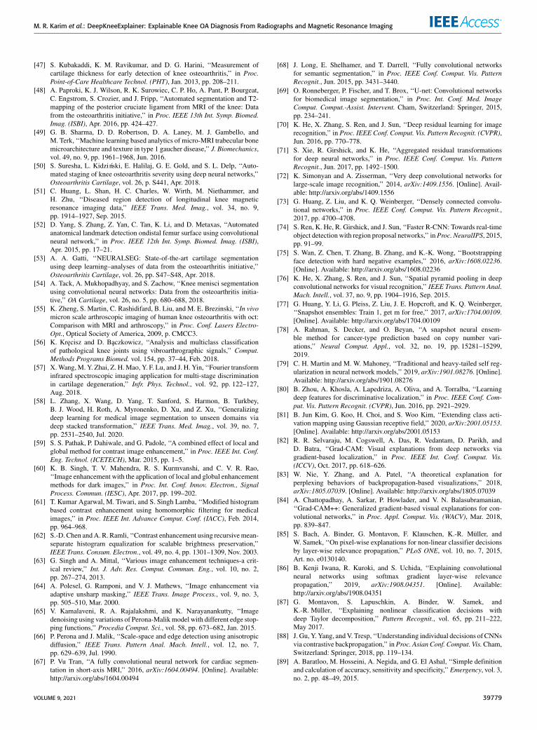
M. R. Karim et al.: DeepKneeExplainer: Explainable Knee OA Diagnosis From Radiographs and Magnetic Resonance Imaging
[47] S. Kubakaddi, K. M. Ravikumar, and D. G. Harini, ‘‘Measurement ofcartilage thickness for early detection of knee osteoarthritis,’’ in Proc.Point-of-Care Healthcare Technol. (PHT), Jan. 2013, pp. 208–211.
[48] A. Paproki, K. J. Wilson, R. K. Surowiec, C. P. Ho, A. Pant, P. Bourgeat,C. Engstrom, S. Crozier, and J. Fripp, ‘‘Automated segmentation and T2-mapping of the posterior cruciate ligament from MRI of the knee: Datafrom the osteoarthritis initiative,’’ in Proc. IEEE 13th Int. Symp. Biomed.Imag. (ISBI), Apr. 2016, pp. 424–427.
[49] G. B. Sharma, D. D. Robertson, D. A. Laney, M. J. Gambello, andM. Terk, ‘‘Machine learning based analytics of micro-MRI trabecular bonemicroarchitecture and texture in type 1 gaucher disease,’’ J. Biomechanics,vol. 49, no. 9, pp. 1961–1968, Jun. 2016.
[50] S. Suresha, L. Kidziński, E. Halilaj, G. E. Gold, and S. L. Delp, ‘‘Auto-mated staging of knee osteoarthritis severity using deep neural networks,’’Osteoarthritis Cartilage, vol. 26, p. S441, Apr. 2018.
[51] C. Huang, L. Shan, H. C. Charles, W. Wirth, M. Niethammer, andH. Zhu, ‘‘Diseased region detection of longitudinal knee magneticresonance imaging data,’’ IEEE Trans. Med. Imag., vol. 34, no. 9,pp. 1914–1927, Sep. 2015.
[52] D. Yang, S. Zhang, Z. Yan, C. Tan, K. Li, and D. Metaxas, ‘‘Automatedanatomical landmark detection ondistal femur surface using convolutionalneural network,’’ in Proc. IEEE 12th Int. Symp. Biomed. Imag. (ISBI),Apr. 2015, pp. 17–21.
[53] A. A. Gatti, ‘‘NEURALSEG: State-of-the-art cartilage segmentationusing deep learning–analyses of data from the osteoarthritis initiative,’’Osteoarthritis Cartilage, vol. 26, pp. S47–S48, Apr. 2018.
[54] A. Tack, A. Mukhopadhyay, and S. Zachow, ‘‘Knee menisci segmentationusing convolutional neural networks: Data from the osteoarthritis initia-tive,’’ OA Cartilage, vol. 26, no. 5, pp. 680–688, 2018.
[55] K. Zheng, S. Martin, C. Rashidifard, B. Liu, and M. E. Brezinski, ‘‘In vivomicron scale arthroscopic imaging of human knee osteoarthritis with oct:Comparison with MRI and arthroscopy,’’ in Proc. Conf. Lasers Electro-Opt., Optical Society of America, 2009, p. CMCC3.
[56] K. Krecisz and D. Baczkowicz, ‘‘Analysis and multiclass classificationof pathological knee joints using vibroarthrographic signals,’’ Comput.Methods Programs Biomed. vol. 154, pp. 37–44, Feb. 2018.
[57] X.Wang,M. Y. Zhai, Z. H.Mao, Y. F. Lu, and J. H. Yin, ‘‘Fourier transforminfrared spectroscopic imaging application for multi-stage discriminationin cartilage degeneration,’’ Infr. Phys. Technol., vol. 92, pp. 122–127,Aug. 2018.
[58] L. Zhang, X. Wang, D. Yang, T. Sanford, S. Harmon, B. Turkbey,B. J. Wood, H. Roth, A. Myronenko, D. Xu, and Z. Xu, ‘‘Generalizingdeep learning for medical image segmentation to unseen domains viadeep stacked transformation,’’ IEEE Trans. Med. Imag., vol. 39, no. 7,pp. 2531–2540, Jul. 2020.
[59] S. S. Pathak, P. Dahiwale, and G. Padole, ‘‘A combined effect of local andglobal method for contrast image enhancement,’’ in Proc. IEEE Int. Conf.Eng. Technol. (ICETECH), Mar. 2015, pp. 1–5.
[60] K. B. Singh, T. V. Mahendra, R. S. Kurmvanshi, and C. V. R. Rao,‘‘Image enhancement with the application of local and global enhancementmethods for dark images,’’ in Proc. Int. Conf. Innov. Electron., SignalProcess. Commun. (IESC), Apr. 2017, pp. 199–202.
[61] T. Kumar Agarwal, M. Tiwari, and S. Singh Lamba, ‘‘Modified histogrambased contrast enhancement using homomorphic filtering for medicalimages,’’ in Proc. IEEE Int. Advance Comput. Conf. (IACC), Feb. 2014,pp. 964–968.
[62] S.-D. Chen andA. R. Ramli, ‘‘Contrast enhancement using recursivemean-separate histogram equalization for scalable brightness preservation,’’IEEE Trans. Consum. Electron., vol. 49, no. 4, pp. 1301–1309, Nov. 2003.
[63] G. Singh and A. Mittal, ‘‘Various image enhancement techniques-a crit-ical review,’’ Int. J. Adv. Res. Comput. Commun. Eng., vol. 10, no. 2,pp. 267–274, 2013.
[64] A. Polesel, G. Ramponi, and V. J. Mathews, ‘‘Image enhancement viaadaptive unsharp masking,’’ IEEE Trans. Image Process., vol. 9, no. 3,pp. 505–510, Mar. 2000.
[65] V. Kamalaveni, R. A. Rajalakshmi, and K. Narayanankutty, ‘‘Imagedenoising using variations of Perona-Malikmodel with different edge stop-ping functions,’’ Procedia Comput. Sci., vol. 58, pp. 673–682, Jan. 2015.
[66] P. Perona and J. Malik, ‘‘Scale-space and edge detection using anisotropicdiffusion,’’ IEEE Trans. Pattern Anal. Mach. Intell., vol. 12, no. 7,pp. 629–639, Jul. 1990.
[67] P. Vu Tran, ‘‘A fully convolutional neural network for cardiac segmen-tation in short-axis MRI,’’ 2016, arXiv:1604.00494. [Online]. Available:http://arxiv.org/abs/1604.00494
[68] J. Long, E. Shelhamer, and T. Darrell, ‘‘Fully convolutional networksfor semantic segmentation,’’ in Proc. IEEE Conf. Comput. Vis. PatternRecognit., Jun. 2015, pp. 3431–3440.
[69] O. Ronneberger, P. Fischer, and T. Brox, ‘‘U-net: Convolutional networksfor biomedical image segmentation,’’ in Proc. Int. Conf. Med. ImageComput. Comput.-Assist. Intervent. Cham, Switzerland: Springer, 2015,pp. 234–241.
[70] K. He, X. Zhang, S. Ren, and J. Sun, ‘‘Deep residual learning for imagerecognition,’’ in Proc. IEEE Conf. Comput. Vis. Pattern Recognit. (CVPR),Jun. 2016, pp. 770–778.
[71] S. Xie, R. Girshick, and K. He, ‘‘Aggregated residual transformationsfor deep neural networks,’’ in Proc. IEEE Conf. Comput. Vis. PatternRecognit., Jun. 2017, pp. 1492–1500.
[72] K. Simonyan and A. Zisserman, ‘‘Very deep convolutional networks forlarge-scale image recognition,’’ 2014, arXiv:1409.1556. [Online]. Avail-able: http://arxiv.org/abs/1409.1556
[73] G. Huang, Z. Liu, and K. Q. Weinberger, ‘‘Densely connected convolu-tional networks,’’ in Proc. IEEE Conf. Comput. Vis. Pattern Recognit.,2017, pp. 4700–4708.
[74] S. Ren, K. He, R. Girshick, and J. Sun, ‘‘Faster R-CNN: Towards real-timeobject detectionwith region proposal networks,’’ inProc. NeuralIPS, 2015,pp. 91–99.
[75] S. Wan, Z. Chen, T. Zhang, B. Zhang, and K.-K. Wong, ‘‘Bootstrappingface detection with hard negative examples,’’ 2016, arXiv:1608.02236.[Online]. Available: http://arxiv.org/abs/1608.02236
[76] K. He, X. Zhang, S. Ren, and J. Sun, ‘‘Spatial pyramid pooling in deepconvolutional networks for visual recognition,’’ IEEE Trans. Pattern Anal.Mach. Intell., vol. 37, no. 9, pp. 1904–1916, Sep. 2015.
[77] G. Huang, Y. Li, G. Pleiss, Z. Liu, J. E. Hopcroft, and K. Q. Weinberger,‘‘Snapshot ensembles: Train 1, get m for free,’’ 2017, arXiv:1704.00109.[Online]. Available: http://arxiv.org/abs/1704.00109
[78] A. Rahman, S. Decker, and O. Beyan, ‘‘A snapshot neural ensem-ble method for cancer-type prediction based on copy number vari-ations,’’ Neural Comput. Appl., vol. 32, no. 19, pp. 15281–15299,2019.
[79] C. H. Martin and M. W. Mahoney, ‘‘Traditional and heavy-tailed self reg-ularization in neural network models,’’ 2019, arXiv:1901.08276. [Online].Available: http://arxiv.org/abs/1901.08276
[80] B. Zhou, A. Khosla, A. Lapedriza, A. Oliva, and A. Torralba, ‘‘Learningdeep features for discriminative localization,’’ in Proc. IEEE Conf. Com-put. Vis. Pattern Recognit. (CVPR), Jun. 2016, pp. 2921–2929.
[81] B. Jun Kim, G. Koo, H. Choi, and S. Woo Kim, ‘‘Extending class acti-vation mapping using Gaussian receptive field,’’ 2020, arXiv:2001.05153.[Online]. Available: http://arxiv.org/abs/2001.05153
[82] R. R. Selvaraju, M. Cogswell, A. Das, R. Vedantam, D. Parikh, andD. Batra, ‘‘Grad-CAM: Visual explanations from deep networks viagradient-based localization,’’ in Proc. IEEE Int. Conf. Comput. Vis.(ICCV), Oct. 2017, pp. 618–626.
[83] W. Nie, Y. Zhang, and A. Patel, ‘‘A theoretical explanation forperplexing behaviors of backpropagation-based visualizations,’’ 2018,arXiv:1805.07039. [Online]. Available: http://arxiv.org/abs/1805.07039
[84] A. Chattopadhay, A. Sarkar, P. Howlader, and V. N. Balasubramanian,‘‘Grad-CAM++: Generalized gradient-based visual explanations for con-volutional networks,’’ in Proc. Appl. Comput. Vis. (WACV), Mar. 2018,pp. 839–847.
[85] S. Bach, A. Binder, G. Montavon, F. Klauschen, K.-R. Müller, andW. Samek, ‘‘On pixel-wise explanations for non-linear classifier decisionsby layer-wise relevance propagation,’’ PLoS ONE, vol. 10, no. 7, 2015,Art. no. e0130140.
[86] B. Kenji Iwana, R. Kuroki, and S. Uchida, ‘‘Explaining convolutionalneural networks using softmax gradient layer-wise relevancepropagation,’’ 2019, arXiv:1908.04351. [Online]. Available:http://arxiv.org/abs/1908.04351
[87] G. Montavon, S. Lapuschkin, A. Binder, W. Samek, andK.-R. Müller, ‘‘Explaining nonlinear classification decisions withdeep Taylor decomposition,’’ Pattern Recognit., vol. 65, pp. 211–222,May 2017.
[88] J. Gu, Y. Yang, andV. Tresp, ‘‘Understanding individual decisions of CNNsvia contrastive backpropagation,’’ inProc. Asian Conf. Comput. Vis.Cham,Switzerland: Springer, 2018, pp. 119–134.
[89] A. Baratloo, M. Hosseini, A. Negida, and G. El Ashal, ‘‘Simple definitionand calculation of accuracy, sensitivity and specificity,’’ Emergency, vol. 3,no. 2, pp. 48–49, 2015.
VOLUME 9, 2021 39779
M. R. Karim et al.: DeepKneeExplainer: Explainable Knee OA Diagnosis From Radiographs and Magnetic Resonance Imaging
[90] N. A. Segal, M. C. Nevitt, K. D. Gross, C. E. Lewis, and J. C. Torner,‘‘The multicenter osteoarthritis study (MOST): Opportunities for rehabil-itation research,’’ PM R, J. Injury, Function, Rehabilitation, vol. 5, no. 8,pp. 1–13, 2013.
[91] H. Lee, S. Yune, M. Mansouri, M. Kim, S. H. Tajmir,C. E. Guerrier, S. A. Ebert, S. R. Pomerantz, J. M. Romero, S. Kamalian,and R. G. Gonzalez, ‘‘An explainable deep-learning algorithm for thedetection of acute intracranial haemorrhage from small datasets,’’ NatureBiomed. Eng., vol. 3, no. 3, pp. 173–182, 2019.
[92] T. Patrick, A. K. Hans, and S. Friedhelm, ‘‘Multimodal deep denoisingconvolutional autoencoders for pain intensity classification based on phys-iological signals,’’ in Proc. Int. Conf. Pattern Recognit. Appl. Methods,2020, pp. 289–296.
[93] M. Liang, Z. Li, T. Chen, and J. Zeng, ‘‘Integrative data analysis of multi-platform cancer data with a multimodal deep learning approach,’’ IEEETrans. Comput. Biol. Bioinf., vol. 12, no. 5, pp. 928–937, Jul./Aug. 2015.
MD. REZAUL KARIM received the M.Sc. degreein computer science from Kyung Hee University,South Korea. He is currently pursuing the Ph.D.degree with RWTH Aachen University, Germany.He is also an Applied and Data Scientist withFraunhofer FIT, Germany. Previously, he workedas a Researcher with the Insight Centre for DataAnalytics, Ireland, and as a Lead Software Engi-neer with Samsung Electronics Company Ltd. Hisresearch interests include machine learning, bioin-
formatics, and explainable artificial intelligence (XAI).
JIAO JIAO received the B.Sc. degree from theBeijing University of Technology, China, and theM.Sc. degree from RWTH Aachen University,Germany. She is currently a Data Scientist withFraunhofer ISI, Germany. Her research interestsinclude explainable AI and text mining.
TILL DÖHMEN received the M.Sc. degree in arti-ficial intelligence from Vrije Universiteit Amster-dam, The Netherlands. He is currently pursuingthe Ph.D. degree with RWTH Aachen Univer-sity, Germany. He is also a Data Science SolutionArchitect with Fraunhofer FIT. His research inter-ests include knowledge graphs, machine learning,and explainable AI.
MICHAEL COCHEZ received the B.Sc. degreein information technology from the Universityof Antwerp, Belgium, and the M.Sc. and Ph.D.degrees in mathematical information technologyfrom the University of Jyväskylä, Finland. He wasformerly a Postdoctoral Researcher with Fraun-hofer FIT. He is currently an Assistant Professorof Artificial Intelligence with Vrije UniversiteitAmsterdam, The Netherlands. His research inter-ests include knowledge representation, machinelearning, and data mining.
OYA BEYAN is currently a Researcher withFraunhofer FIT and RWTH Aachen University,Germany. At Fraunhofer FIT, she’s leading the‘‘FAIR Data & Distributed Analytics’’ group.Her research interests include methods of datareusability and FAIR data, data-driven transforma-tion, and distributed analytics.
DIETRICH REBHOLZ-SCHUHMANN was for-merly the Director of the Insight Centre for DataAnalytics and a Professor with NUI Galway,Ireland. He is currently a Professor of medicinewith the University of Cologne and the Scien-tific Director of the German National Libraryof Medicine (ZB MED), Cologne, Germany. Hisresearch interests include data science, semanticsdriven data analytics, biomedical data mining, andbioinformatics.
STEFAN DECKER was formerly a Professor andthe Director of the Insight Centre for Data Analyt-ics, NUI Galway, Ireland. He is currently the Man-aging Director of Fraunhofer FIT and a Professorof Computer Science with RWTHAachen Univer-sity, Germany. His research interests include infor-mation systems, semantic web and linked data,data science, and knowledge representation.
39780 VOLUME 9, 2021
Related Documents