Experimentally uncertainty quantiﬁcation in numerical … · Experimentally uncertainty quantiﬁcation in numerical and ... to ensure short design cycles while dealing with low

Experimentally uncertainty quantification in numerical andanalytical beam models

P. Langer1; K. Sepahvand2; M. Krause3; S. Marburg2

1,2 Universität der Bundeswehr Munich, 85579 Neubiberg, Germany3 Isko-engineers AG, 80807 Munich, Germany

ABSTRACTIn modern industrial processes such as developing new products, virtual prototyping is state of the art methodto ensure short design cycles while dealing with low cost pressure. In order to meet these criteria, efficient andreliable simulations must be available. Numerical methods, especially the Finite Element Method (FEM) arecommonly used in various industrial fields e.g. the automotive sector, aircraft design and ship construction.The scope of this paper is to enhance the reliability of numerical models utilizing FEM when consideringuncertain parameters of the underlying structure. Such parameters can be system related, i.e. geometry, materialbehavior, boundary conditions and mesh density as well as general assumptions in the process of modeling.Two well-known beam theories, i. e. Euler-Bernoulli and Timoshenko theory, have been utilized. At FElevel, various elements available for modeling of beam structures in ABAQUS have been compared andevaluated. Experimental modal analysis have been performed on beam specimen to validate the results fromanalytical and FE models due to parameter uncertainties. A comparison between the numerical and analyticalsimulations with experiments reveal the element types with minimum deviation with regard to parameteruncertainties. Having sufficient knowledge of the dynamic behavior of simple beam samples, the complexitywill be increased. This investigation developed instructions on how detailed a numerical model must be builtto get satisfactory results.

Keywords: Uncertainty quantification, FE modeling, beam structures, experimental modal analysis

1. INTRODUCTIONA model is an abstraction of reality in which many assumptions are made. It is not possible to evaluate

correct results without knowing the underlying assumptions (1, 2). For this reason it is important to find exactlythe right model that is the most suitable for the conceptual formulation. In the formation of the mathematicalmodels the minimum description length principle (MDL) proposed by Rissanen (3) is one useful approachto finding the shortest description of the data and the model itself. Ross Quinlan and Rives provide a gooddescription of MDL principle in (4). The method, however, does not include the estimation of errors in theresults.Model building and simulation are becoming increasingly important in engineering. In simulation phase, theFinite Element Method (FEM) is manly used to construct a numerical model. Within the past decade increasingin computer capability, FEM has become highly important in model formation for engineers. Additionally,in industry, FEM has crucial importance for reducing the number of experimental examinations. The majorissue is that every FEM model possess some degree of uncertainty due to topological and material parameters,initial and boundary conditions, forcing term, etc. The results from FEM models are trustable if they arevalidated with experimental or results from available analytical models. When comparing the models, however,uncertainties must be taken into account. General recommendations regarding model uncertainties are givenin (5) that are important for model formation and in the development process. A powerful tool in numericalsimulation of engineering problems involve uncertainty is the stochastic finite element method (SFEM), whichis an extension of deterministic FEM in random framework (6). The application of the method on variouspractical engineering problems including uncertainty has been studied in many works, cf. (7, 8, 9, 10, 11, 12)This paper present a comparison of numerical, analytical models and the experimental results for beamstructures involving material and parameter uncertainties. The results have been studied for various quadratictetrahedral and hexahedral elements types with different number of elements to realize the model uncertainties.

[email protected]

Inter-noise 2014 Page 1 of 10

[email protected]

Page 2 of 10 Inter-noise 2014

The one–dimensional solution obtained by Euler–Bernoulli and Timoshenko was used for the analyses in thisstudy. The physical model for experimental results depends on the precision of the measuring equipment andthe apparatus used to perform an experiment. The considered uncertainties include material and shape, whilemodel uncertainties include boundary conditions, model assumptions, model depth and level of detail. Themodel depth, is, by definition, the formation of elements, and the level of detail is the number of elements. Theinvestigation includes a study of the model depth and the level of detail in which the FE model is verified forthe analytical solution is first described, this is followed by verification for an overkill calculation. The physical,numerical and analytical models will be compared using the best regular mesh determined. Later, when themodels get more complexity, it is not possible to mesh the whole geometrical irregularities. Therefore, theinfluence of distortion in numerical mesh is investigated. A recommendation is given since a virtual image forexactly one simple real shape can be made. Abaqus/CAE was used as a pre- and postprocessor for this task. Inthe experimental modal analysis, the free–free beam specimens were contact free excited by a periodic chirpsignal by means of loudspeakers. The resonance frequencies of the first 3 bending modes were measured witha Laser–Doppler–Vibrometer.The remainder of the paper is organized as follows. Section 2 reviews the investigated FEM, analytical andexperimental models. The numerical simulations of the method illustrate in section 3. Section 4 discusses theconclusions.

2. MODEL DESCRIPTIONIn this section, we discuss the details of FEM, analytical and experimental models considered in the

investigation.

2.1 FEM modelsFor this study the model was created in Abaqus/CAE and submitted to the Abaqus/standard implicit solver.

Various types of elements in the mesh module can be selected in the Abaqus element library. Table 1 showsthe elements that were available for the study.

Table 1 – Element description from elements, that were selected in the Abaqus element library for thestudy (13).

Name Nodes Basis function General marks

C3D20 20 quadratic three dimensional quadratic brickC3D20R 20 quadratic three dimensional quadratic brick with reduced integrationC3D20H 20 quadratic three dimensional quadratic brick with linear pressure formulationC3D10 10 quadratic three dimensional tetrahedronC3D10M 10 quadratic three dimensional tetrahedron with hourglass controlC3D10I 10 quadratic three dimensional tetrahedron with improved stress visualizationC3D10H 10 quadratic three dimensional tetrahedron with linear pressure formulationC3D8 8 linear three dimensional linear brick

All elements have a quadratic formulation function because linear formulation functions stiffen the structureat bending. The highest possible precision of the models are investigated and compared in this study.

2.2 Analytical ModelsThe analytical model is based on two well–known Euler–Bernoulli and Timoshenko beam theories. The

Euler–Bernoulli beam theory assumes no shear deflection and rotary inertia. For this reason the Timoshenkotheory is formulated to cover this drawbacks. This theory also includes assumptions. One of these is that, theshear stress distribution across the cross section is assumed to be constant and linear. It is also assumed thatthe cross–sectional area is symmetric so that the neutral and centroidal axes coincide. A comprehensive studyon various beam theories is given in (14). Although many high–order beam theories are available, they will bedisregarded here. The analytical solutions lead to one–dimensional equations, which does not represent manyphysical effects on the structure. That must be clear for the results.

2.3 Physical Models and ExperimentsThe physical model uses experimental modal analysis in which beam samples were suspended from two

elastic strings and activated acoustically with a periodic chirp signal by a loudspeaker. A chirp is a signal inwhich frequency increases or decreases over time. Measurements are carried out in an anechoic chamber to



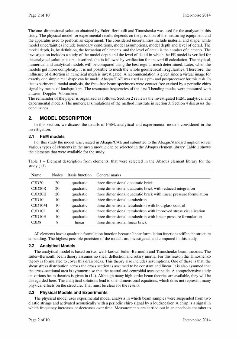
avoid the influence of acoustic reflections from the walls. The microphone measures effective sound pressuregenerated by the loudspeaker to find the input value for the FRF. The deflection shape was measured by aLaser–Doppler–Vibrometer in front of the beam shape. Figure 1 shows the measuring setup seen from theVibrometer: microphone (1), the loudspeaker (2), beam shape (3), elastic strings (4) and anechoic chamber (5).The eigenfrequencies and the associated bending modes were found numerically using ME’scope.

1

2

3

4 5

Figure 1 – Experimental setup of beam samples, suspended by means of two elastic strings and excitatoryacoustically with a periodic chirp signal by a loudspeaker.

3. RESULTSIn this section the study results are presented. The beam samples are made of steel and aluminum and

homogeneous and elastic material properties were assumed. The nominal values of uncertain material andgeometrical parameters of 10 beam samples are given in Table 2. The deviation of the density for the 10

Table 2 – The nominal values of uncertain geometrical and material parameters.

Parameter Steel Aluminum

Length, L [mm] 200 200Width, B [mm] 40 40Thickness, H [mm] 4 4Density [kgm−3] 7817 2663Young’s modulus [Gpa] 211 72Poisson’s ratio [-] 0.30 0.34

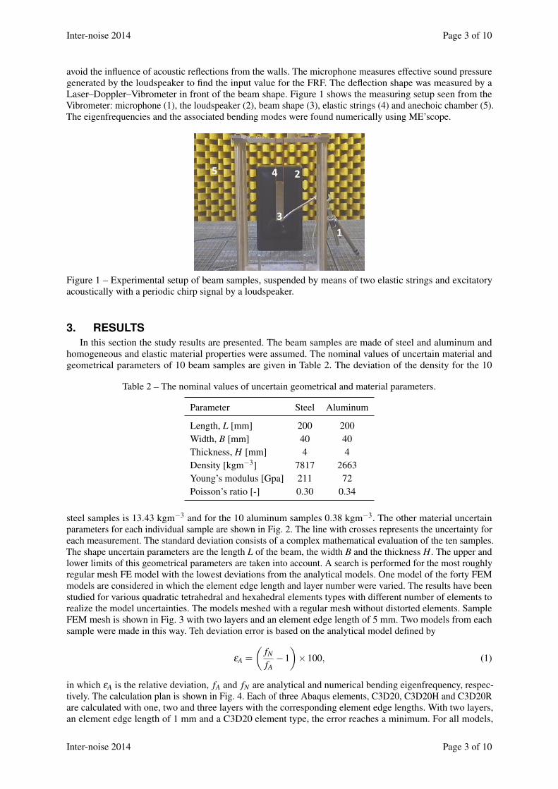
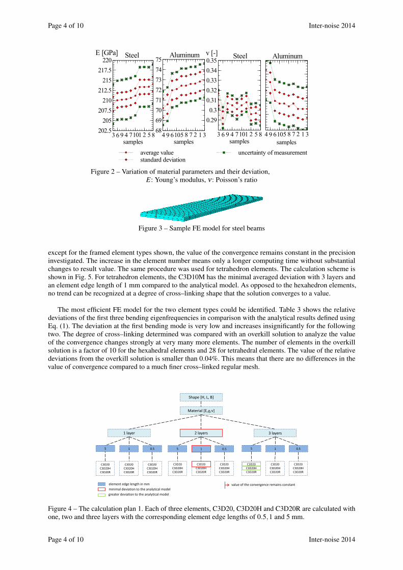
steel samples is 13.43 kgm−3 and for the 10 aluminum samples 0.38 kgm−3. The other material uncertainparameters for each individual sample are shown in Fig. 2. The line with crosses represents the uncertainty foreach measurement. The standard deviation consists of a complex mathematical evaluation of the ten samples.The shape uncertain parameters are the length L of the beam, the width B and the thickness H. The upper andlower limits of this geometrical parameters are taken into account. A search is performed for the most roughlyregular mesh FE model with the lowest deviations from the analytical models. One model of the forty FEMmodels are considered in which the element edge length and layer number were varied. The results have beenstudied for various quadratic tetrahedral and hexahedral elements types with different number of elements torealize the model uncertainties. The models meshed with a regular mesh without distorted elements. SampleFEM mesh is shown in Fig. 3 with two layers and an element edge length of 5 mm. Two models from eachsample were made in this way. Teh deviation error is based on the analytical model defined by

εA =

(fN

fA−1

)×100, (1)

in which εA is the relative deviation, fA and fN are analytical and numerical bending eigenfrequency, respec-tively. The calculation plan is shown in Fig. 4. Each of three Abaqus elements, C3D20, C3D20H and C3D20Rare calculated with one, two and three layers with the corresponding element edge lengths. With two layers,an element edge length of 1 mm and a C3D20 element type, the error reaches a minimum. For all models,



Steel Aluminum

851 2107493 6

v [-] AluminumSteel

0.290.3

0.310.320.330.340.35

samples317 2851064 9

6869707172737475

samples317 2851064 9

samples851 2107493 6

E [GPa]

average valuestandard deviation

uncertainty of measurement

202.5205

207.5210

212.5215

217.5220

samples

Figure 2 – Variation of material parameters and their deviation,E: Young’s modulus, ν : Poisson’s ratio

Figure 3 – Sample FE model for steel beams

except for the framed element types shown, the value of the convergence remains constant in the precisioninvestigated. The increase in the element number means only a longer computing time without substantialchanges to result value. The same procedure was used for tetrahedron elements. The calculation scheme isshown in Fig. 5. For tetrahedron elements, the C3D10M has the minimal averaged deviation with 3 layers andan element edge length of 1 mm compared to the analytical model. As opposed to the hexahedron elements,no trend can be recognized at a degree of cross–linking shape that the solution converges to a value.

The most efficient FE model for the two element types could be identified. Table 3 shows the relativedeviations of the first three bending eigenfrequencies in comparison with the analytical results defined usingEq. (1). The deviation at the first bending mode is very low and increases insignificantly for the followingtwo. The degree of cross–linking determined was compared with an overkill solution to analyze the valueof the convergence changes strongly at very many more elements. The number of elements in the overkillsolution is a factor of 10 for the hexahedral elements and 28 for tetrahedral elements. The value of the relativedeviations from the overkill solution is smaller than 0.04%. This means that there are no differences in thevalue of convergence compared to a much finer cross–linked regular mesh.

F

Shape [H, L, B]

Material [E,ϱ,ν]

1 layer 2 layers 3 layers

5 1 0.5 5 1 0.5 5 1 0.5

C3D20 C3D20H C3D20R

C3D20 C3D20H C3D20R

C3D20 C3D20H C3D20R

C3D20 C3D20H C3D20R

C3D20 C3D20H C3D20R

C3D20 C3D20H C3D20R

C3D20 C3D20H C3D20R

C3D20 C3D20H C3D20R

C3D20 C3D20H C3D20R

minimal deviation to the analytical model value of the convergence remains constant

greater deviation to the analytical model

element edge length in mm

Figure 4 – The calculation plan 1. Each of three elements, C3D20, C3D20H and C3D20R are calculated withone, two and three layers with the corresponding element edge lengths of 0.5,1 and 5 mm.



F

Shape [H, L, B]

Material [E,ϱ,ν]

2 layers 3 layers 4 layers

5 1 0.8 5 1 0.8 5 1 0.8

C3D10 C3D10H C3D10M C3D10I









minimal middle deviation to the analytical model

element edge length in mm

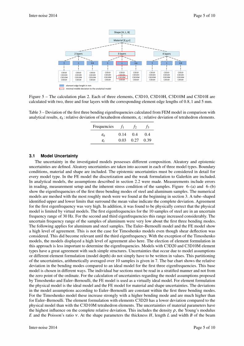
Figure 5 – The calculation plan 2. Each of three elements, C3D10, C3D10H, C3D10M and C3D10I arecalculated with two, three and four layers with the corresponding element edge lengths of 0.8,1 and 5 mm.

Table 3 – Deviation of the first three bending eigenfrequencies calculated from FEM model in comparison withanalytical results, εh : relative deviation of hexahedron elements, εt : relative deviation of tetrahedron elements.

Frequencies f1 f2 f3

εh 0.14 0.4 0.4εt 0.03 0.27 0.39

3.1 Model UncertaintyThe uncertainty in the investigated models possesses different composition. Aleatory and epistemic

uncertainties are defined. Aleatory uncertainties are taken into account in each of three model types. Boundaryconditions, material and shape are included. The epistemic uncertainties must be considered in detail forevery model type. In the FE model the discretization and the weak formulation to Galerkin are included.In analytical models, the assumptions described in section 2.2 were made. Measurements include errorsin reading, measurement setup and the inherent stress condition of the samples. Figure 6–(a) and 6–(b)show the eigenfrequencies of the first three bending modes of steel and aluminum samples. The numericalmodels are meshed with the most roughly mesh were we found at the beginning in section 3. A tube–shapedidentified upper and lower limits that surround the mean value indicate the complete deviation. Agreementfor the first eigenfrequency was very high. In addition, it was found to be physically correct that the physicalmodel is limited by virtual models. The first eigenfrequencies for the 10 samples of steel are in an uncertainfrequency range of 30 Hz. For the second and third eigenfrequencies this range increased considerably. Theuncertain frequency range of the samples of aluminum were very low about the first three bending modes.The following applies for aluminum and steel samples. The Euler–Bernoulli model and the FE model showa high level of agreement. This is not the case for Timoshenko models even though shear deflection wasconsidered. This did become relevant until the third eigenfrequency. With the exception of the Timoshenkomodels, the models displayed a high level of agreement also here. The election of element formulation inthis approach is less important to determine the eigenfrequencies. Models with C3D20 and C3D10M elementtypes have a great agreement with such simple structures. Uncertainties that occur due to model assumptionsor different element formulation (model depth) do not simply have to be written in values. This partitioningof the uncertainties, arithmetically averaged over 10 samples is given in 7. The bar chart shows the relativedeviation in the bending modes compared to an ideal model for the first three eigenfrequencies. This basemodel is chosen in different ways. The individual bar sections must be read in a stratified manner and not fromthe zero point of the ordinate. For the calculation of uncertainties regarding the model assumptions proposedby Timoshenko and Euler–Bernoulli, the FE model is used as a virtually ideal model. For element formulationthe physical model is the ideal model and the FE model for material and shape uncertainties. The deviationsin the model assumptions according to Euler–Bernoulli are constant within the first three bending modes.For the Timoshenko model these increase strongly with a higher bending mode and are much higher thanfor Euler–Bernoulli. The element formulation with elements C3D20 has a lower deviation compared to thephysical model than with the C3D10M tetrahedron elements. The uncertainties of material parameters havethe highest influence on the complete relative deviation. This includes the density ρ , the Young’s modulusE and the Poisson’s ratio ν . At the shape parameters the thickness H, length L and width B of the beam



third bending mode

second bending mode

first bending mode

39610147852

f [H

z]

2800290030003100

samples

f [H

z]

1450147515001525155015751600

BernoulliTimoshenko

LDVC3D20

C3D10M

f [H

z]

530540550560570

(a)

third bending mode

second bending mode

first bending mode

94610728135

f [H

z]

27502800285029002950

samples

f [H

z]

1400142014401460148015001520

BernoulliTimoshenko

LDVC3D20

C3D10M

f [H

z]

515520525530535540545

(b)

Figure 6 – The first three eigenfrequencies of the bending modes with uncertainties. (a): steel samples, (b):aluminum samples

were analyzed. The relative deviation in material parameters and shape parameters is constant for the firstthree eigenfrequencies of the bending modes. With the exception of an analytical Timoshenko beam, the totaldeviation remains constant as the bending modes increase.

Timoshenko

C3D10MC3D20

rela

tive

devi

atio

n [%

]

−2

−1

0

1

2

numbers of bending modes3.2.1.

Steel

Bernoulli - model assumption vs. numerical solutionTimoshenko - model assumption vs. numerical solutionC3D20 - model assumption vs. experimentC3D10M - model assumption vs. experimentmaterialshape

Figure 7 – Individual uncertainties about 10 samples – arithmetic mean values – stacked.

3.2 Influence of distorted elementsThe purpose of this section is to analyze the influence of distorted mesh elements on the total numerical

errors. For simple beam structures, distorted mesh have been analysed on the total numerical errors. Forthe mesh of simple numerical models of beam structures, distorted elements could be avoided. For morecomplex structures that can not be excluded, therefore it is important for the next steps of the work to know theinfluence of distorted elements exactly to the numerical solution. Lee and Bathe (15) classified the distortionof two–dimensional elements in six different categories, which are shown in figure 8. In Fig. 8–(a), a squareelement with evenly spaced nodes is shown as the undistorted element. In Fig. 8–(b), the distortion is thecause of very high aspect ratio in direction of the two coordinates r and s. Lee and Bathe defined in figure8–(c) a state of distortion due to the unequal position of the nodes on the element edges. The displacement ofthe element node to a parallelogram is shown in figure 8–(d). In figure 8–(e) the element is distorted due to acurved edge. Figure 8–(f) shows a distorted element by the large and small angle between two element edgeswith a common node. As Lee and Bathe described, The same principle as described by Lee and Bathe is used



(a) (b) (c)

(d) (e) (f)

s

r

s

r

s

r

s

r

s

r

s

r

Figure 8 – Classification of two-dimensional element distortion (15)

in Abaqus/CAE mesh verification feature to check the quality of mesh elements. For each critical/distortedelement either a warning or an error message is reported. In the former case, despite the warning message,Abaqus solver is capable of handling the model. When the criteria exceed a certain level, however, an errormessage is displayed and Abaqus solver cannot be started. The verification part of the mesh in Abaqus checksthe quality of the elements and gives for each critical element a warning or an error. In the first case, themodel for the solver of Abaqus remains solvable. If these criteria are injured too much, Abaqus issues an errormessage and the solver can not be started.In Abaqus, the surface is differentiated in form and size criteria. Two sub-criteria are used for this study: Theangle criterion and a geometric deviation factor. The former considers the angle between two element edgesthat converge in a node. For angles larger than 10 degrees, no warning or error messages are issued. Thegeometric deviation factor is defined by

delement

lelement< 0.2, (2)

in which delement is the distance between the the distorted and undistorted states of the element edge and lelementis the length of this element edge. The limits for each criterion can be changed in Abaqus manually.

𝐸𝑠 ↓↓ 𝐸𝑠 ↑↑ 𝐸𝑠 ↓↓

𝐸𝑠 ↓↓ 𝐸𝑠 ↑↑ 𝐸𝑠 ↓↓ 𝐸𝑠 ↓↓ 𝐸𝑠 ↑↑

Figure 9 – Total elastic strain energy Es for the first and second bending mode; mesh: 1 layer, 5 mm elementedge length; top: first bending mode; bottom: second bending mode



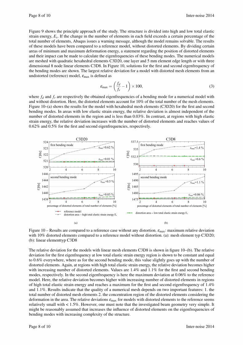
Figure 9 shows the principle approach of the study. The structure is divided into high and low total elasticstrain energy, Es. If the change in the number of elements in each field exceeds a certain percentage of thetotal number of elements, Abaqus issues a warning message, although the model remains solvable. The resultsof these models have been compared to a reference model, without distorted elements. By dividing certainareas of minimum and maximum deformation energy, a statement regarding the position of distorted elementsand their impact can be made to calculate the eigenfrequencies of these bending modes. The numerical modelsare meshed with quadratic hexahedral elements C3D20, one layer and 5 mm element edge length or with threedimensional 8 node linear elements C3D8. In Figure 10, solutions for the first and second eigenfrequency ofthe bending modes are shown. The largest relative deviation for a model with distorted mesh elements from anundistorted (reference) model, εmax is defined as

εmax =

(fd

fr−1

)×100, (3)

where fd and fr are respectively the obtained eigenfrequencies of a bending mode for a numerical model withand without distortion. Here, the distorted elements account for 10% of the total number of the mesh elements.Figure 10–(a) shows the results for the model with hexahedral mesh elements (C3D20) for the first and secondbending modes. In areas with low elastic strain energy, the relative deviation is almost independent of thenumber of distorted elements in the region and is less than 0.03%. In contrast, at regions with high elasticstrain energy, the relative deviation increases with the number of distorted elements and reaches values of0.62% and 0.5% for the first and second eigenfrequencies, respectively.

C3D20

εmax=0.5 %

εmax=0.03 %

second bending mode

f ]H

z]

1438

1440

1442

1444

1446

percentage of distorted elements of total number of elements [%]2 4 6 8 10

εmax=0.62 %

εmax=0.01 %

reference modeldistortion area -- high total elastic strain energy Es

first bending mode

f ]H

z]

520

521

522

523

524

2 4 6 8 10

(a)

C3D8

εmax=1.1 %

εmax=0.06 %

second bending mode

f ]H

z]

1475

1480

1485

1490

1495

percentage of distorted elements of total number of elements [%]2 4 6 8 10

εmax=0.6 %

εmax=1.4 %

distortion area -- low total elastic strain energy Es

first bending mode

f ]H

z]

530

532.5

535

537.5

2 4 6 8 10

(b)

Figure 10 – Results are compared to a reference case without any distortion. εmax: maximum relative deviationwith 10% distorted elements compared to a reference model without distortion. (a): mesh element typ C3D20;(b): linear elementtyp C3D8

The relative deviation for the models with linear mesh elements C3D8 is shown in figure 10–(b). The relativedeviation for the first eigenfrequency at low total elastic strain energy region is shown to be constant and equalto 0.6% everywhere, where as for the second bending mode, this value slightly goes up with the number ofdistorted elements. Again, at regions with high total elastic strain energy, the relative deviation becomes higherwith increasing number of distorted elements. Values are 1.4% and 1.1% for the first and second bendingmodes, respectively. In the second eigenfrequency is here the maximum deviation at 0.06% to the referencemodel. Here, the relative deviation becomes higher with increasing number of distorted elements in regionsof high total elastic strain energy and reaches a maximum for the first and second eigenfrequency of 1.4%and 1.1%. Results indicate that the quality of a numerical mesh depends on two important features: 1. thetotal number of distorted mesh elements 2. the concentration region of the distorted elements considering thedeformation in the area. The relative deviations εmax for models with distorted elements to the reference seemsrelatively small with < 1.5%. However, one must note that the investigated beam geometry very simple. Itmight be reasonably assumed that increases the influence of distorted elements on the eigenfrequencies ofbending modes with increasing complexity of the structure.



3.3 Comparison to experimental modelsIn this section the FE models for which the most efficient mesh for hexahedral and tetrahedral elements

were found, the Euler–Bernoulli beam and Timoshenko beam are compared with reality, that is results fromexperimental modal analysis. Material and shape parameters are mean average values. Figure 11 shows therelative deviation, εP , from experimental (physical) model defined as

εP =

(fn/a

fe−1

)×100, (4)

where fn/a and fe are the numerical/analytical and experimental bending eigenfrequencies. The results for10 models made of steel over the abscissa are connected by lines and colored areas. An area that signifies acomplete deviation for more than 10 samples results for every model type. The surface sections must be readin a stratified manner and not from the zero point of the ordinate. The FE model with the hexahedral elementformulation C3D20 has the lowest relative deviation from the physical model. The deviation decreases evenmore with increasingly higher bending modes. The arithmetic mean values of relative deviation for more than10 samples and the first three eigenfrequencies of bending modes is −0.06%, −0.07% and −0.05%. For theFE model with the C3D10M element type the following deviations were determined: −0.18%, −0.21% and−0.19%. The FE solution for a model with hexahedron elements, an element edge length of 1 mm and a layernumber of 2 are thus closer to physical model. This can be clearly seen by the surface representation in Figure11. The Euler–Bernoulli model still show a good agreement compared the physical model. With increasinglyhigher bending mode the Timoshenko model has the largest deviations from the physical model. Figure 11shows the same results, but for the 10 models made of aluminium. Comparing FE models with the C3D20

39610147852

Steel (C45)

C3D20C3D10M

TimoshenkoBernoulli

ε P [%

]

−4−3

01

samples

ε P [%

]

−4−3−2−1

012

third bending mode

second bending mode

first bending mode

ε P [%

]

−3−2−1

0123

(a)

44610728135

Aluminum (ENAW)

C3D20C3D10M

TimoshenkoBernoulli

ε P [%

]

−5−4

01

samples

ε P [%

]

−4−3−2−1

01

third bending mode

second bending mode

first bending mode

ε P [%

]

−3−2−1

0123

(b)

Figure 11 – Relative deviation about 10 samples to physical model - stacked area. (a): steel samples, (b):aluminum samples

and C3D10M element formulations reveals interesting results. Unlike the steel samples the model is closerto the physical model with the tetrahedron mesh. The arithmetic mean values of relative deviation for morethan 10 samples for the first three eigenfrequencies of bending modes is 0.25%, 0.14% and 0.13%. For theFE model with the C3D20 element type, the deviations were 0.38%, 0.27% and 0.26%. Euler–Bernoulli andTimoshenko beams behave in a similar fashion as in the case of steel samples.



4. CONCLUSIONSThis paper has attempted to provide a recommendation regarding the level of discretization in FE models

with simple structures at which results converge. It provides the engineer with certainty regarding the sufficientnumber degrees of freedom in simple beam structures. An element type for this case was proposed. It wasshown that uncertainties regarding material and shape parameters always have a considerable influence on theeigenfrequencies of bending modes. The uncertainties for the model assumptions according Timoshenko werethe only ones that had a significant increase with the bending modes. Numerical, physical and analytical modelshave a high level agreement up to the third eigenfrequency of the bending modes. It is shown analytical models,this does not converge absolutely to a better result despite a high–order beam theory. In these examinations thesimpler Euler–Bernoulli model has a higher agreement with the physical and FE models. The comparison tophysical models shows that the FE models have the lowest deviation to the reality. For steel samples the mostaccurate element type is C3D20. Otherwise, for aluminum samples the tetrahedron elements C3D10M. Theinfluence of distorted mesh elements on the total numerical errors has been investigated. Results indicated thatthe quality of a numerical mesh depends on the total number of distorted mesh elements and the concentrationregion of the distorted elements considering the deformation in the area. It is demonstrated that mesh areaswith low elastic strain energy, the relative deviation is almost independent of the number of distorted elementsin the region. This is in contrast to regions with high elastic strain energy where the relative deviation increaseswith the number of distorted elements.

REFERENCES1. Balci O. Credibility Assessment of Simulation Results: The State of the Art. In: Eastern Simulation

Conferences. Orlando, Fla.; 1987. p. 1–8.

2. Sevgi L. Modeling and Simulation Concepts in Engineering Education: Virtual Tools. Turkish Journal ofElectrical Engineering and Computer Sciences. 2006;14(1):113–12.

3. Rissanen J. An Introduction to the MDL Principle. Helsinki Institute for Information Technology; Tampereand Helsinki Universities of Technology, Finland, and University of London, England;.

4. Quinlan JR, Rives RL. Inferring Decision Trees Unsing the Minimum Description Length Principle.Massachusetts: Academic Press; 1989.

5. Sargent G. Verification and Validation of Simulation Models. In: Winter Simulation Conferences. Orlando;2005. p. 53–59.

6. Stefanou G. The stochastic finite element method: Past, present and future. Computer Methods in AppliedMechanics and Engineering. 2009;198(9–12):1031–1051.

7. Li R, Ghanem R. Adaptive polynomial chaos expansions applied to statistics of extremes in nonlinearrandom vibration. Probabilistic Engineering Mechanics. 1998;13(2):125–136.

8. Lucor D, Su CH, Karniadakis GE. Generalized polynomial chaos and random oscillators. InternationalJournal for Numerical Methods in Engineering. 2004;60(3):571–596.

9. Soize C. A comprehensive overview of a non–parametric probabilistic approach of model uncertaintiesfor predictive models in structural dynamics. Journal of Sound and Vibration. 2005;288(3):623–652.

10. Sepahvand K, Marburg S, Hardtke HJ. Stochastic free vibration of orthotropic plates using generalizedpolynomial chaos expansion. Journal of Sound and Vibration. 2012;331(1):167–179.

11. Marburg S, Beer HJ, Gier J, Hardtke HJ. Experimental verification of structural–acoustic modelling anddesign optimization. Journal of Sound and Vibration. 2002;252(4):591–615.

12. Sephavand K, Marburg S. On construction of uncertain material parameter using generalized polynomialchaos expansion from experimental data. In: IUTAM Symposium on Multiscale Problems in StochasticMechanics. Karlsruhe; 2012. p. 4–17.

13. Abaqus User and Theory Manual 6.10-3;.

14. Han SM, Benaroya H, Wei T. Dynamics of transversely vibrating beams using four engineering theories.Journal of Sound and Vibration. 1999;225(5):935 – 988.

15. Lee NS, Bathe KJ. Effects of Element distortions on the performance of isoparametric elements. Interna-tional Journal for numerical Methods in engineering. 1993;36:3553–3576.


Experimentally uncertainty quantiﬁcation in numerical … · Experimentally uncertainty quantiﬁcation in numerical and ... to ensure short design cycles while dealing with low

Documents