Experimental studies to overcome the recycling barriers of ...

Doctoral Thesis in Material Science and Engineering

Experimental studies to overcome the recycling barriers of stainless-steel and BOF slagsMATTIA DE COLLE

Stockholm, Sweden 2022

kth royal institute of technology

Experimental studies to overcome the recycling barriers of stainless-steel and BOF slagsMATTIA DE COLLE

Doctoral Thesis in Material Science and EngineeringKTH Royal Institute of TechnologyStockholm, Sweden 2022

Academic Dissertation which, with due permission of the KTH Royal Institute of Technology, is submitted for public defence for the Degree of Doctor of Philosophy on Friday the 11th of March 2022, Stockholm.

© Mattia De Colle ISBN 978-91-8040-123-4TRITA – ITM-AVL 2022:1 Printed by: Universitetsservice US-AB, Sweden 2022

Abstract

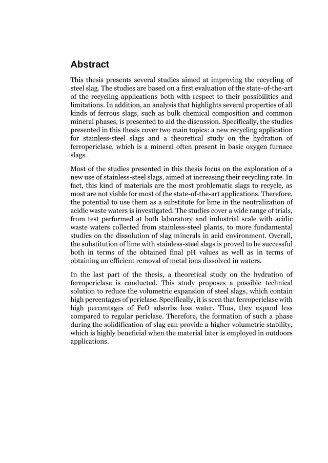
This thesis presents several studies aimed at improving the recycling of

steel slag. The studies are based on a first evaluation of the state-of-the-art

of the recycling applications both with respect to their possibilities and

limitations. In addition, an analysis that highlights several properties of all

kinds of ferrous slags, such as bulk chemical composition and common

mineral phases, is presented to aid the discussion. Specifically, the studies

presented in this thesis cover two main topics: a new recycling application

for stainless-steel slags and a theoretical study on the hydration of

ferropericlase, which is a mineral often present in basic oxygen furnace

slags.

Most of the studies presented in this thesis focus on the exploration of a

new use of stainless-steel slags, aimed at increasing their recycling rate. In

fact, this kind of materials are the most problematic slags to recycle, as

most are not viable for most of the state-of-the-art applications. Therefore,

the potential to use them as a substitute for lime in the neutralization of

acidic waste waters is investigated. The studies cover a wide range of trials,

from test performed at both laboratory and industrial scale with acidic

waste waters collected from stainless-steel plants, to more fundamental

studies on the dissolution of slag minerals in acid environment. Overall,

the substitution of lime with stainless-steel slags is proved to be successful

both in terms of the obtained final pH values as well as in terms of

obtaining an efficient removal of metal ions dissolved in waters.

In the last part of the thesis, a theoretical study on the hydration of

ferropericlase is conducted. This study proposes a possible technical

solution to reduce the volumetric expansion of steel slags, which contain

high percentages of periclase. Specifically, it is seen that ferropericlase with

high percentages of FeO adsorbs less water. Thus, they expand less

compared to regular periclase. Therefore, the formation of such a phase

during the solidification of slag can provide a higher volumetric stability,

which is highly beneficial when the material later is employed in outdoors

applications.

Sammanfattning

Denna avhandling presenterar flera studier som syftar till att förbättra

återvinningen av stålslagger. Studierna är baserade på en första

utvärdering av den senaste tekniken för återvinningsapplikationer både

med avseende på möjligheter och begränsningar. Dessutom presenteras en

studie som belyser flera egenskaper hos alla typer av järnslagger, såsom

bulk-kemisk sammansättning och vanliga mineralfaser, för att underlätta

diskussionen. Specifikt, så omfattar studierna som presenteras i denna

avhandling två huvudämnen: en ny återvinningsapplikation för slagger

från tillverkning av rostfritt stål och en teoretisk studie om hydrering av

ferroperiklas, vilket är ett mineral som ofta förekommer i konverterslagger.

De flesta av de studier som presenteras i denna avhandling fokuserar på

utforskningen av en ny användning av slagger från tillverkning av rostfritt

stål, i syfte att undersöka hur det är möjligt att öka deras återvinningsgrad.

Faktum är att denna typ av material är de mest problematiska slaggerna

att återvinna, eftersom de flesta inte kan behandlas med användandet av

de flesta av de senaste slaggåtervinningsteknikerna. Därför undersöks

deras potential att kunna användas som ersättning för kalk vid

neutralisering av surt avloppsvatten. Studierna omfattar ett brett spektrum

av försök, från laboratorietester till industriella tester med surt

avloppsvatten som samlats från rostfria ståltillverkningsanläggningar, till

mer grundläggande studier om hur upplösning av slaggmineraler sker i en

sur miljö. Sammanfattningsvis, så visar resultaten att ersättningen av kalk

med slagg av rostfritt stål är framgångsrik både med avseende på att

slutliga pH-värden som erhållits samt med avseende på att erhålla ett

effektivt avlägsnande av metalljoner som är lösta i vatten.

I sista delen av avhandlingen så behandlas en teoretisk studie om

hydrering av ferroperiklas. Denna studie föreslår en möjlig teknisk

lösning för att minska den volymetriska expansionen av stålslagg som

innehåller höga halter av periklas. Specifikt så visar resultaten att

ferroperiklas med höga andelar FeO adsorberar mindre vatten och därför

så expanderar dessa slagger mindre i jämförelse med vanlig ferroperiklas.

Därför kan bildandet av en sådan fas under stelning av slagg ge en högre

volymetrisk stabilitet, vilket är mycket fördelaktigt när materialet senare

används i applikationer utomhus.

Acknowledgements

This PhD thesis is only the final step of a journey that saw numerous people

involved, both directly and indirectly. To them I owe my deepest gratitude.

I hope the following few words will be a sufficient token of my appreciation.

I would like to begin by thanking my supervisors Pär G. Jönsson for his

constant positive attitude, general guidance and support and Andrey

Karasev for his rigorous approach to science, valuable feedbacks and

discussions. A warm thank you to Alicia Gauffin too, who introduced me to

the topic and guided me in the first months of my doctorate. Finally, thank

you all for selecting me for this project, giving me this great opportunity.

The success of my studies is also merit of many people outside the

academic community: Gunnar Ruist, Olle Sundqvist, Robert Eriksson and

all the members of TO55 have been crucial in supporting me in carrying

out my studies. The financial support from Jernkontoret is also gratefully

acknowledged.

My sincere gratitude to Shibata sensei, Sukenaga sensei and all the

members of their team, for the wonderful experience that has been living

and working in Sendai. I’ll always cherish your warmth and friendliness in

welcoming me in your team. The work conducted in Japan has been an

insightful experience that tremendously helped me in my growth as a

researcher. Thank you also to David, Guglielmo, and Oscar for such crazy

adventures and wonderful time spent together there.

Thanks to all the people I met through THS MAIN and the International

Reception. Working in those associations have been a crucial part of my

growth as a person. A special mention goes to Federico, Pablo, Alessandro,

Parastu, Albin and Adam for such wonderful experiences and friendship.

Thanks to Lorenzo and Silvia, which made the workplace a more cheerful

and lively environment throughout the years.

To my unofficial brother Paolo and sister Freddie. You had been a major

part of my life in the latest years, giving me plenty of moments to be

extremely grateful for. I hope our friendship will continue through the

borders of our respective countries.

I wish to thank all my long time Italian friends for making my hometown

over these years my favorite place to come back to and the hardest one to

leave. Alfonso, Davide, Filippo, Gabriele, Gherardo, Valentina and

Veronica, thank you for simply all this time spent together.

Lastly, thanks to my mom and dad that never questioned, rather always

supported, my life choices even when they made no sense to them.

Stockholm, December 2021

Mattia De Colle

Supplements

The following supplements have been used for the writing of this thesis:

Supplement 1: De Colle, M. et al. The Use of High-Alloyed EAF Slag for the Neutralization of On-Site Produced Acidic Wastewater: The First Step Towards a Zero-Waste Stainless-Steel Production Process. Appl. Sci. 9, 3974 (2019).

Supplement 2: De Colle, M., Jönsson, P., Gauffin, A. & Karasev, A. Optimizing the use of EAF stainless steel Slag to neutralize acid baths. in Proceedings of the 6th International Slag Valorisation Symposium, 1-5 April 2019, Mechelen, Belgium: Science, Innovation & Entrepreneurship in Pursuit of a Sustainable World (KU Leuven, Materials Engineering, 2019).

Supplement 3: De Colle, M., Kielman, R., Karlsson, A., Karasev, A. & Jönsson, P. G. Study of the Dissolution of Stainless-Steel Slag Minerals in Different Acid Environments to Promote Their Use for the Treatment of Acidic Wastewaters. Appl. Sci. 11, 12106 (2021).

Supplement 4: De Colle, M., Puthucode, R., Karasev, A. & Jönsson, P. G. A Study of Treatment of Industrial Acidic Wastewaters with Stainless Steel Slags Using Pilot Trials. Materials 14, 4806 (2021).

Supplement 5: De Colle, M. et al. Study of the Hydration Behavior of Synthetic ferropericlase with Low Iron Oxide Concentrations to Prevent Swelling in Steel Slags. J. Sustain. Metall. (2021) doi:10.1007/s40831-021-00359-x.

The contribution of the main author of this thesis to the supplements is the

following:

Supplement 1: Literature survey, design of the experimental methods,

sample preparation, performing of the pH buffering trials, general data

analysis and major part of the writing.


part of the sample preparation, performing of the pH buffering trials,

general data analysis and major part of the writing.

Supplement 3: Part of the literature survey, design of the experimental

methods, part of the sample preparation, performing of the pH buffering

trials, most of the XRD analysis, some of the SEM-EDS analysis, general

data analysis and major part of the writing.


performing of the pH buffering trials, general data analysis and major part

of the writing.

Supplement 5: Literature survey, part of the design of the experimental

methods, mineral synthesis, autoclave curing, XRD analysis, TGA analysis,

general data analysis and major part of the writing

List of Tables

• Table 1: Schematic representation of how the experimental setup of each supplement is related by topic, factors impeding the recycling of slag and proposed solutions.

• Table 2: Summary of the experimental methods used from Supplement 1 to Supplement 4

• Table 3: Material code and description of the slag samples used in the pH buffering studies

• Table 4: Compound name, chemical formula and crystal system of each mineral found in the slag samples

• Table 5: Stepwise dosing method applied with powders sifted through a mesh of 1mm and 63µm.

• Table 6: Results of the ICP tests. tracing 6 elements in water samples treated with either slag O1 or lime. The pre-treatment values and the threshold values admitted by the Swedish law are also used a reference.

• Table 7: Mixing time trials with probe positions in A & B

• Table 8: Mixing time trials with probe positions C & D and A & E

• Table 9: Up-scaled stepwise dosing trials characteristics (liters, rpm, total mass of added slag, and final pH value).

• Table 10: TGA trials performed on periclase samples after hydration with autoclave curing.

• Table 11: TGA results after the hydration of the sintered samples performed with autoclave curing

• Table 12: Main findings of each study related to the initial experimental setup and proposed solution

List of Figures

• Figure 1: Schematic of the iron and steelmaking processes with relative slag production

• Figure 2: A schematic representation of a stepwise dosing trial with three additions of reactant

• Figure 3: A schematic representation of a single-step dosing trial with one addition of reactant.

• Figure 4: Graphical example of how mixing time can be calculated given the ratio Ci/Cfinal over time.

• Figure 5: Semi-quantitative analysis of the mineral phases, expressed as % of the total, of the four slag samples O1, S1, O2 and S2.

• Figure 6: Amount in wt% of the most abundant elements of all the slag samples

• Figure 7: PSD of the slag samples after being crushed and sieved through 1 mm mesh

• Figure 8: Laboratory single-step trials with slag sample O1 and S1 sieved through a 1 mm mesh

• Figure 9: Laboratory single-step trials with lime samples from OTK and SVK

• Figure 10: Laboratory single-step trials with slag sample O1, S1 and O2 after ball-milling and sieving through a 63 µm mesh

• Figure 11: Single-step dosing trials of a 0.1M HCl solution performed with 0.5, 1 and 2 g of slag samples O1, S1, O2 and S2 (grouped slag type).

• Figure 12: Single-step dosing trials of a 0.1M HCl solution performed with the slag samples S1, O1, O2 (grouped by added slag weight of 1g and 2g)

• Figure 13: Single-step dosing trials of a 0.1 M solution of HCl performed with 0.5g and 0.25g of CaO

• Figure 14: Single-step dosing trials of the 0.1 M HCl and HNO3 acid solutions performed with 1 g of slag samples S1 and O1 on the left, and O2 and S2 on the right.

• Figure 15: XRD spectra of the residues extracted after the single-step trials of a 0.1M HCl solution performed with 0.25g and 0.5 g of CaO. The peaks related with the phase CaCl2*nH2O are highlighted by dots at their respective peaks.

• Figure 16: XRD spectra of the residues extracted after the single-step trials of a 0.1M HCl solution performed with the slag samples S1, O1, O2 and S2.

• Figure 17: XRD spectra of the residues extracted after the single-step trials of a 0.1M HCl solution performed with 0.25g of CaO and 1g of slag samples S1, O1 and O2. The peaks related with the phase CaCl2*nH2O are highlighted by dots at their respective peaks

• Figure 18: Up-scaled single-step dosing trials with 90L and 70L of wastewaters and slag O1

• Figure 19: BSE images of the cut surface of pellets of the samples 10 wt% FeO (a), 15 wt% FeO (b) and 20 wt% FeO (c).

• Figure 20: XRD spectra of the sintered samples. FP and MF peaks are used as reference to evaluate the samples’ composition.

• Figure 21: Mössbauer spectra of all the samples with velocity from -4 to 4 mm/s on the left, with velocity from -12 to 12 mm/s on the right. Four sites are identified and each contribution to the total spectra is unbundled. The sites are grouped into the phases of origin. The global spectra are also presented (black marker and long-dotted red line). The black arrows point the comparable peak position for the Fe3+site in the FP phase in a previous study84. Yellow markers are used to identify the MF peaks (full marker: peaks that were visible in the -4, +4 mm/s range).

• Figure 22: TG (straight-blue) and T°C (dotted-red) curve obtained during the dehydration of standard grade sample of brucite

• Figure 23: XRD spectra of the sample with 15 wt% of FeO after sintering, autoclave curing, and TGA.

• Figure 24: Pourbaix diagrams (10-6 M) calculated in Factsage 6.1 89. (A) Ca, (B) Mg, (C) Al and (D) Si 81.

• Figure 25: XRD spectra of the residues extracted after the single-step trials of a 0.1M HCl solution performed with 1g and 2g of slag O2. The intensities are normalized to a 100 to aid a proper comparison between the spectra.

• Figure 26: Linear regression of L/S ratio of the 90 L and 70 L single-step dosing trials. L/S ratios belonging to the precedent single-step dosing trials have been added for comparison.

• Figure 27: Reduction of sample weight (ΔW%) after TGA analyses on the hydrated samples plotted as a function of the calculated Fe2+ at%. The dash-dotted line represents the hydration behavior of an unsintered powder mixture consisting of MgO and FeO, where MgO is fully transformed in brucite and FeO acts as bulk material. The dotted line represents the linear regression of all TGA measurements. For comparison, a data point of composition 80mol%MgO−20mol%FeO from the study made by Hou at al. 77 has been added.

List Of Abbreviations

BOF Basic oxygen furnace BF Blast Furnace EAF Electric Arc Furnace AOD Argon oxygen decarburization f-CaO Free CaO f-MgO Free MgO PSD Particle size distribution L/S Liquid to solid FP Ferropericlase OTK Outokumpu Stainless AB SVK Sandvik Materials Technology AB SEM Scanning electron microscope XRD X-ray Powder Diffraction ICP Inductively coupled plasma EDS Energy-dispersive X-ray spectroscopy Tm Mixing time EPMA Electron Probe Micro Analyzer Fe3+ Trivalent Iron Fe2+ Bivalent Iron TGA Thermogravimetric analysis BSE Back-scattered electron MF Magnesioferrite

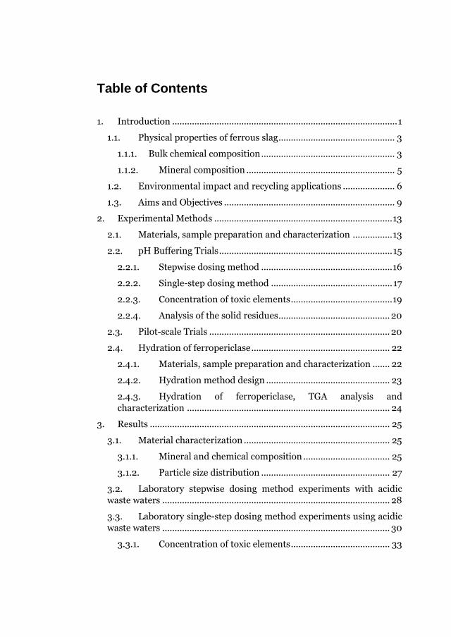
Table of Contents

1. Introduction ........................................................................................... 1

1.1. Physical properties of ferrous slag ............................................... 3

1.1.1. Bulk chemical composition ...................................................... 3

1.1.2. Mineral composition ............................................................ 5

1.2. Environmental impact and recycling applications ..................... 6

1.3. Aims and Objectives ..................................................................... 9

2. Experimental Methods ........................................................................ 13

2.1. Materials, sample preparation and characterization ................ 13

2.2. pH Buffering Trials ...................................................................... 15

2.2.1. Stepwise dosing method ..................................................... 16

2.2.2. Single-step dosing method ................................................. 17

2.2.3. Concentration of toxic elements ......................................... 19

2.2.4. Analysis of the solid residues ............................................. 20

2.3. Pilot-scale Trials ......................................................................... 20

2.4. Hydration of ferropericlase ........................................................ 22

2.4.1. Materials, sample preparation and characterization ....... 22

2.4.2. Hydration method design .................................................. 23

2.4.3. Hydration of ferropericlase, TGA analysis and

characterization .................................................................................. 24

3. Results ................................................................................................. 25

3.1. Material characterization ........................................................... 25

3.1.1. Mineral and chemical composition ................................... 25

3.1.2. Particle size distribution .................................................... 27

3.2. Laboratory stepwise dosing method experiments with acidic

waste waters ............................................................................................ 28

3.3. Laboratory single-step dosing method experiments using acidic

waste waters ............................................................................................ 30

3.3.1. Concentration of toxic elements ........................................ 33

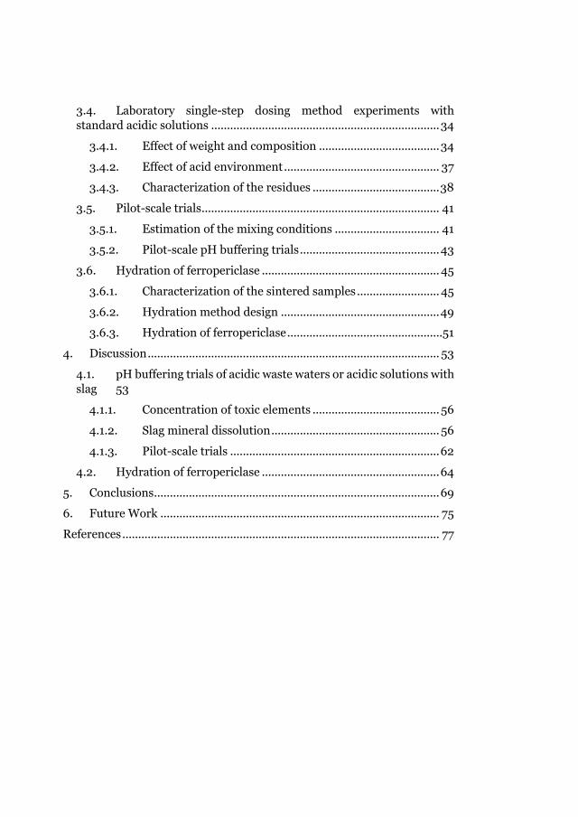
3.4. Laboratory single-step dosing method experiments with

standard acidic solutions ........................................................................ 34

3.4.1. Effect of weight and composition ...................................... 34

3.4.2. Effect of acid environment ................................................. 37

3.4.3. Characterization of the residues ........................................ 38

3.5. Pilot-scale trials ........................................................................... 41

3.5.1. Estimation of the mixing conditions ................................. 41

3.5.2. Pilot-scale pH buffering trials ............................................ 43


3.6.1. Characterization of the sintered samples .......................... 45

3.6.2. Hydration method design .................................................. 49

3.6.3. Hydration of ferropericlase .................................................51

4. Discussion ............................................................................................ 53

4.1. pH buffering trials of acidic waste waters or acidic solutions with

slag 53

4.1.1. Concentration of toxic elements ........................................ 56

4.1.2. Slag mineral dissolution ..................................................... 56

4.1.3. Pilot-scale trials .................................................................. 62


5. Conclusions.......................................................................................... 69

6. Future Work ........................................................................................ 75

References .................................................................................................... 77

1 | Introduction

1. Introduction

Slag is a broad term used to the define the most abundant by-products

generated during the smelting and production of metals. All metallurgical

slags are chemical compounds consisting of many different types of oxides

and metallic inclusions. This is due to the intrinsic nature of slags. In fact,

when metal elements oxidized during the smelting or production of metals,

they float to the surface of the metal bath due to their reduced densities.

Furthermore, slag is not only formed by the oxidation of elements present

in the metal bath, but also due to chemical reactions with several minerals

(generally called flux, flux agents or slag formers) injected during various

steps of the metal productions, that perform different roles. In fact, flux

agents are not only used to protect the metals from the atmosphere, but

also to insulate the molten bath, so that heat losses are avoided. Although,

more importantly their composition ensures the transfer of elements

between the metal bath and the slag, refining the composition of the final

product to the desired targets. Moreover, since the production of metals is

a such a ubiquitous and variegated industry, this category of materials

presents a wide range of bulk chemical compositions and mineral

structures. Thus, this variance makes studying these materials, and their

applications, quite complex if done holistically. Therefore, there’s a need to

define further subcategories that can describe groups of slags with more

homogenous features.

Slag by-products are usually divided into two big categories, namely

ferrous and nonferrous slags. Nonferrous slags are produced by the

smelting and the recovery of nonferrous metals. Specifically, the most

important ones being copper, nickel, phosphorous, lead, and zinc. In this

category the many different materials present a high variance in chemical

and mineral composition, but due to the low production volumes of each

kind of slag, they are often grouped together. Meanwhile, ferrous slags are

the by-products associated with the production of iron and steel. This class

of materials is more homogenous compared to the one related to

nonferrous slags and overshadows the first in terms of generated volumes.

Thus, ferrous slags are treated as a single category. In fact, according to

Yildirim et al.1 0.25 to 0.30 tons of slag are generated per ton of pig iron.

In case of steel, the author claims that the ratio changes to 0.2.

Furthermore, if the recovery of basic oxygen furnace (BOF) slags as flux

agent in the blast furnace (BF) is accounted for, the ratio diminishes to

0.10-0.15 of the total output of steel. However, another source indicates

that in the case of stainless-steel slag the ratio is 0.30 per ton of steel

Introduction | 2

produced2. This translates to roughly 260-300 Mt of iron slags and 150-

220 Mt of steel slags produced worldwide in 2011. In Europe, the European

steel association “Eurofer” estimates that 42 Mt of slags are produced3.

Holappa et al.4 estimate in their review that roughly 600 Mt of slag were

produced by the iron a steel industry in 2019, of which 52 Mt from the

stainless steel production. This numbers are also similar to situation in the

US, where in 2011 the production of steel slag amounted to 10-15 Mt a year,

with a landfilling rate of 15-40%1.

Ferrous slags can be divided into even smaller subcategories, namely iron

slags and steel slags. Iron slags are associated with the production of pig

iron, so they mainly consist of BF slags. On the other hand, depending on

the different furnaces where they are generated, steel slags present distinct

chemical compositions. Specifically, if steel is produced starting from

primary sources, BOF slags are produced. Contrary, if steel is produced by

remelting metal scraps, Electric Arc Furnace (EAF) slag is generated.

Common to both routes of production, the steel composition is further

controlled in the ladle, with the consequent generation of ladle slags, which

also shows different chemical composition compared to the previous two

kinds of slags. One additional step usually characterizes the production of

stainless-steel slags, which is the use of an Argon Oxygen Decarburization

(AOD) converter, which also generates its namesake slag. How the various

steps relate to each other, along with the input materials used, is shown in

Figure 1. As it is possible to notice, flux agents are added at each step of the

steelmaking and iron processes. The quantity and the chemical

composition of these minerals may vary, but the most used are usually lime

or dolomitic lime. Other minerals such as alumina or silica or sources of

several alloying elements can also be included. Stainless steel is a classic

example of this, containing high amounts of Ni and Cr. Coke is also used,

but it is limited to the production of pig iron. The composition of the

metallic melt also varies substantially depending on the step of the process.

For instance, pig iron has a very high carbon content, around 4%, whereas

steel contains carbon contents vary from 2% to very low percentages,

depending on the requirements of the final products. Moreover, stainless

steel usually has a carbon content lower that 1%. In general, it can be said

that depending on the initial composition of the input materials and the

target composition at the end of the process, the chemical reactions which

take place between flux agents and the metallic melt are substantially

different. For instance, despite that steel is produced both in the EAF and

BOF reactors, the reactions happening during the two processes vary

substantially. All these factors reflect on the bulk composition of slag,

3 | Introduction

which will show distinct composition differences depending on which

furnace produces it. This thesis will focus on describing more in detail

ferrous slags, with a particular attention to BOF slags and stainless-steel

slags, as the studies conducted involve those kinds of materials.

Figure 1: Schematic of the iron and steelmaking processes with relative slag production

1.1. Physical properties of ferrous slag

1.1.1. Bulk chemical composition

The bulk chemical composition is common to all ferrous slags, containing

mostly Ca and Si along with Fe, Mg and Al. Despite the ranges varies, all

the ferrous slags can be described mostly by these five elements. Usually

the compositions of slag are expressed in terms of their oxides forms, so

that they can be plotted on ternary diagrams, either using a CaO-SiO2-

Al2O3 system or a CaO-SiO2-FeO system5. In other studies, (CaO+MgO)-

SiO2-(Al2O3+FeOx+CrOx) was also used to classify stainless-steel slags2.

Although, as mentioned before, the input materials, the different ratio of

flux agents and the chemical reactions that take place in the various

furnaces all contribute to the production of different slags, which populate

different regions of the ternary diagrams as a result. For instance, BF slags

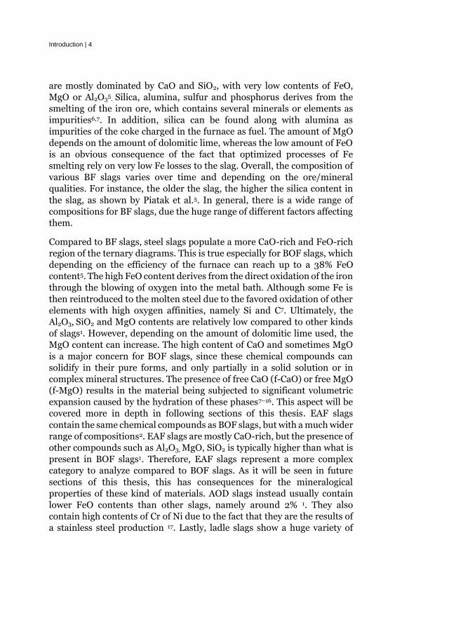
Introduction | 4

are mostly dominated by CaO and SiO2, with very low contents of FeO,

MgO or Al2O35

. Silica, alumina, sulfur and phosphorus derives from the

smelting of the iron ore, which contains several minerals or elements as

impurities6,7. In addition, silica can be found along with alumina as

impurities of the coke charged in the furnace as fuel. The amount of MgO

depends on the amount of dolomitic lime, whereas the low amount of FeO

is an obvious consequence of the fact that optimized processes of Fe

smelting rely on very low Fe losses to the slag. Overall, the composition of

various BF slags varies over time and depending on the ore/mineral

qualities. For instance, the older the slag, the higher the silica content in

the slag, as shown by Piatak et al.5. In general, there is a wide range of

compositions for BF slags, due the huge range of different factors affecting

them.

Compared to BF slags, steel slags populate a more CaO-rich and FeO-rich

region of the ternary diagrams. This is true especially for BOF slags, which

depending on the efficiency of the furnace can reach up to a 38% FeO

content5. The high FeO content derives from the direct oxidation of the iron

through the blowing of oxygen into the metal bath. Although some Fe is

then reintroduced to the molten steel due to the favored oxidation of other

elements with high oxygen affinities, namely Si and C7. Ultimately, the

Al2O3, SiO2 and MgO contents are relatively low compared to other kinds

of slags1. However, depending on the amount of dolomitic lime used, the

MgO content can increase. The high content of CaO and sometimes MgO

is a major concern for BOF slags, since these chemical compounds can

solidify in their pure forms, and only partially in a solid solution or in

complex mineral structures. The presence of free CaO (f-CaO) or free MgO

(f-MgO) results in the material being subjected to significant volumetric

expansion caused by the hydration of these phases7–16. This aspect will be

covered more in depth in following sections of this thesis. EAF slags

contain the same chemical compounds as BOF slags, but with a much wider

range of compositions2. EAF slags are mostly CaO-rich, but the presence of

other compounds such as Al2O3, MgO, SiO2 is typically higher than what is

present in BOF slags1. Therefore, EAF slags represent a more complex

category to analyze compared to BOF slags. As it will be seen in future

sections of this thesis, this has consequences for the mineralogical

properties of these kind of materials. AOD slags instead usually contain

lower FeO contents than other slags, namely around 2% 1. They also

contain high contents of Cr of Ni due to the fact that they are the results of

a stainless steel production 17. Lastly, ladle slags show a huge variety of

5 | Introduction

compositions, and not many studies have been focused on studying their

recycling potential as a separate category1,2,5.

1.1.2. Mineral composition

Highlighting the typical mineral phases present in different kind of slags is

more difficult than determining their bulk chemical compositions. There

are several parameters that cause a wide variety of minerals to form. In

fact, beside the variations in composition, how the slag solidifies affects the

formation of the mineral phases, which is vastly dictated by the cooling

conditions. Moreover, cooling also determines the morphological

properties of the slag, such as the structure, grain size and porosity6.

Different cooling methods are employed for ferrous slags and their choices

is mostly dependent on the final use of the product. For instance, BF slags

can either be air cooled, granulated or expanded6. Air cooled slags are the

ones where the solidification happens due to the cooling in a slag pit in an

open environment, whereas granulated or expanded slags are the results

of quenching with different mixtures of air and water. The changing in

cooling is fundamental to the change in the physical properties of BF slags.

Granulated slags are mostly glassy and dense, whereas air cooled slags

have a high porosity due to the presence of trapped gasses in the solid

matrix. Expanded BF slags are instead more lightweight, and have

different fire resistance and insulation properties than the other two slags6.

Also in the case of steel slags, the formation of glassy phases in BOF and

EAF slag was investigated by Tossavainen et al.18. They showed that BOF

and EAF slags appear to remain crystalline even when subjected to fast

rates of cooling, while presenting similar mineral structures as the original

samples. Another study by Reddy et al.19 investigated how the hydraulic

properties of BOF slags were influenced by the cooling rate of the material.

The study found that depending on the cooling rate, the compressive

strength of the materials changed depending on the cooling conditions. In

addition, in both studies it was reported that the material disintegrates

when dicalcium silicate β turns into dicalcium silicate γ. However, this

phenomenon only occurred for specific compositions and cooling rates18,19.

The combination of the raw chemical compositions and cooling rates

applied determine the mineral phases present in ferrous slags. Piatak et al.5

classify the phases found by the number of occurrences in the different

several studies they analyzed. Minerals belonging to the olivine-group,

which present the general formula (Ca, Fe, Mg, Mn)2*SiO4, are by far the

most re-occurring ones in the studies reviewed, with larnite and

monticellite as the most frequent. This is because most of the studies

Introduction | 6

included in the review focused on the compositions of steel slags, rather

than BF slags. Forsterite and fayalite are also frequent minerals found in

ferrous slags. Another very common phase present in ferrous slags, but

especially in steel slags, are various free oxides of different element, such

as Ca, Mg, Mn, and Fe. As discussed before, the widespread use of lime as

a flux agent and the oxidation of Fe in steelmaking, make those phases

particularly frequent in BOF and EAF slags. Melilite is also a frequent

mineral (either as gehlenite or åkermanite) in BF slags and to a lesser

extent in steel slags. Glass is also present in different compositions and

mostly in BF slags. Spinel phases are also very common mostly in steel

slags. Similar analyses, which investigated the average composition of

stainless-steel slags, confirmed these results and additionally showed that

Cr and Ni, solidify forming Cr-Fe-Ni spinels1. In stainless-steel slags, Cr

and Fe mostly bound as oxides, while Ni was found mostly in metallic

form2,17. The presence in stainless-steel slags of calcium silicates, metallic

oxides, bredigite, merwinite and spinel phase was also confirmed in the

review made by Holappa et. al4.

1.2. Environmental impact and recycling applications

The scientific interest for metallurgical slags has been steadily increasing

since the 1990’s. The studies have been concentrating on two main issues,

namely the environmental impact of these materials and their recycling

applications5. The more conscious humankind becomes on the impact of

the manufacturing sector on the natural environment, and the challenges

that production of goods faces in the nearby future20, the more these kind

of topics are investigated. Moreover, more interest is put in an efficient use

of by-products thanks to the newly born field of circular economy21. Many

scholars have been focusing on conceptualizing a more sustainable and

resource-conservative manufacturing sector22–25, both through the

development of new sustainable business models and by promoting a

paradigm shift which considers waste strictly as a resource to use. A

particularly interesting topic is the implementation of industrial

symbiosis26, which studies the flow of materials/by-products and energy in

a mutually advantageous way. The benefits from this kind of approach are

many, from the lower generation of waste to the reduced need of natural

resources. This translates both in monetary gains for the industries, given

the development of successful technologies, business models and adequate

legislation. It also constitutes a societal benefit since it contributes to

reduce the environmental impact of the manufacturing sector.

7 | Introduction

The technology beyond the recycling of BF slags is quite old and well

established. The materials nowadays are well employed as construction

material, either as concrete or asphalt aggregates. Many BF or steel slags

are dense and hard and they offer great mechanical properties when used

as construction materials, often surpassing natural minerals6,10,27. Contrary

to that, the research focusing on the recycling steel slags is still not so well

established and standard practices application are scarce5. In fact, not all

slags can be safely employed as construction materials. For instance,

Eurofer claims that of the 42 Mt of slag produced in 2019, only which 34

Mt were currently recycled, 65% of which are produced by the production

of iron and 35% from steel3. Jernkontoret, the Swedish steel agency,

published in 2018 a report that indicated the various recycling percentages

per type of slag 28. This report shows that BF and BOF slags are fully or

almost fully recycled in Sweden. The same applies for low alloyed steel

slags produced in the EAF. On the other hand, stainless steel slags coming

from both AOD and EAF processes are mostly landfilled, along with ladle

slags. By comparing the absolute numbers together, despite stainless-steel

slags are approximately the 20% of the total production, they constitute

roughly 80% of the landfilled output in Sweden. The specific difficulties in

recycling stainless-steel slags, compared to low-alloyed ones, are also

highlighted by Holappa et al. 4.

The difficulty in recycling several slags products, and in general their

environmental impact, is mostly caused by the chemical reactions

happening when these materials are subjected to weathering. The contact

with water, or simply the air humidity, can cause mineral changes over

time that impedes some slag products to be successfully employed in

recycling applications. One effect of weathering is on the volumetric

stability. BOF and EAF slags may contain f-CaO or f-MgO, depending on

the process specifications and use of flux agents. These phases hydrates by

absorbing a water molecule per molecule of oxide. This translates into a

volumetric expansion that causes cracks. These fractures expose more

surfaces to weathering, triggering a feedback loop which ultimately

damages the final products in which slags are employed7–16. Several

alternatives have been developed to combat the volumetric stability9,11,13–

16, such as accelerated aging techniques or selective solidification to obtain

hydrophobic phases. However, despite the multiple approaches, in many

cases a complete recycling nor a state-of-the-art solution are yet not

acquired.

The second effect of weathering is commonly known as leaching, which can

be defined as the release of soluble substances from the mineral structures

Introduction | 8

to the outside environment. Leaching is the biggest concern for slags,

especially for steel slags which contains high contents of cancerogenic

elements such Cr and Ni. Nowadays the environmental impact of slags,

even the one disposed, is limited by tight regulations and environmental

practices related to landfills. However, some studies on old slag deposits

show how impactful those materials are when left untreated 29–33. To study

this phenomenon, standard regulations for leaching tests have been

developed. These tests are commonly used to determine whether a material

is classified as hazardous or nonhazardous. This determines whether the

material can be disposed in landfills with or without treatment or

employed for construction materials. Leaching tests consists of batch

experiments where slag is mixed with water. For instance, EN 12457-2 is a

common standard used in Sweden and overall in Europe34, where slag is

ground to a particle size distribution (PSD) <4mm and mixed with

deionized water in a liquid to solid (L/S) ratio of 10 to 1 for 24h. The

concentration of released elements in a liquid phase is then analyzed and

compared to the threshold values allowed by the law. Some studies in the

literature utilize these standards to test the leaching behavior of different

slags and to determine how modification of their structures influence their

leaching35,36. In the literature there are also examples that aim at

simulating dynamic conditions far away from equilibrium leaching, in

attempt to mimic the natural weathering conditions33,37–39. Moreover,

more theoretical studies have been conducted to understand the leaching

mechanisms of steel slags. The development of geochemical models have

been used to predict the transfer of ions, simulating weathering and predict

the long term stability, matching the results with laboratory tests 35,39–41.

Leaching of slags is therefore a deeply studied topic. However, due to its

complexity, the recycling of certain steel slags is still falling short.

The leaching of slag although can be exploited with the right technological

application. Metal recovery is an important part of valorizing slags,

especially for stainless-steel slags which contain high concentrations of

precious metals such as Ni, Cr, Mo, and V. Their tendency to leach these

metals can then be used to extract them from the minerals or from the slag,

if they are present as metallic inclusion. The field of hydrometallurgy has

been conducted several studies focusing on this aspect, with profitable

extractions of Cr and other high valued metals42–44. Another way in which

leaching can be exploited, which will be a major focus of this thesis, is the

use of slag for the neutralization of acidic waste waters. In fact, leachates

from metallurgical slags are usually alkaline due to a high presence of Ca

and Mg. This means that slags can be used for neutralization of acidic

9 | Introduction

solutions and substitute the use of lime, which is currently the common

reactant used in the industry. Several attempts have already been made:

Cunha et al.45,46 used different oxidic by-products, that included some slag

samples, for the neutralization of standard acidic solutions. Also, Forsido

et al.47used a mixture of lime and EAF dust to treat industrial acidic waste

waters, rising both the pH to neutral/basic values, while also removing

metallic ions dissolved in the waters. Lastly, Zvimba et al.48 used BOF slags

for passive neutralization and metallic ions removal of acidic mine

drainage. Developing this technology further can potential be a solution for

slags that currently cannot be safely employed in state-of-the-art

applications as construction materials.

1.3. Aims and Objectives

The current work aims at proposing either new alternatives to valorize

unrecycled steel slags, or to improve their use in current applications. As

previously mentioned, there are several factors impeding a complete, or

even partial, valorization of the materials in the conventional recycling

applications. Among those, the leaching of toxic elements such as Ni and

Cr impedes the use of slags which contain these elements in high levels 4

(such as stainless-steel slags). On the other hand, the presence of f-CaO or

f-MgO in BOF slags shortens the lifespan of the products where these kinds

of materials are employed. In fact, the mineral phases present swell when

coming in contact with water, phenomenon that often causes cracks and

an accelerates failures in use7–16.

The current work covers two distinct projects focusing on the recycling of

steel slags: a novel application for stainless-steel slags, such as their use as

reactants for the pH buffering of acidic wastewaters, and a standalone

study on the hydration of ferropericlase (FP), a mineral which is present in

BOF slags. The first topic is the main part of this work, and it is covered by

supplements from 1 to 4. The investigation is divided into a preliminary

pilot study (Supplement 1), where the experimental methods is developed

in a laboratory setting. In the study, four different slags are tested as pH

buffering agents of industrial acidic wastewaters. Supplement 2 is focused

on improving the investigation methods, mostly by reducing and

homogenizing the particle size distribution, in a way that the materials are

comparable within each other. Thereafter, the effect of the mineral

composition and their influence on the pH of standard acidic solutions is

studied in Supplement 3. Finally, the scalability of this novel application is

tested in Supplement 4, where pilot-scale trials are firstly developed using

a physical model at KTH Royal Institute of Technology. Then, pH buffering

Introduction | 10

trials are conducted at a pilot-scale level at Outokumpu Stainless AB

(Avesta, Sweden).

Supplement 5 studies the hydration properties of several synthetic samples

of FP, a mineral that is often present in BOF slags. The objective of this

work was to improve the recycling of BOF slags, which often is impeded by

the swelling of the material. There are several alternatives that can be

employed to reduce the swelling of the mineral phases 9,11,13–16. Reducing

the formation of f-MgO and f-CaO, in favor of other ones, is the one this

project focuses on. Therefore, the project was conducted to determine how

the water absorption of FP varies, when the percentage of Fe is increased.

FP is a mineral phase already found in BOF slags 49, thus the solidification

of slag could be directed towards the formation of such a phase, rather than

the formation of more hydrophilic phases such as MgO.

11 | Introduction

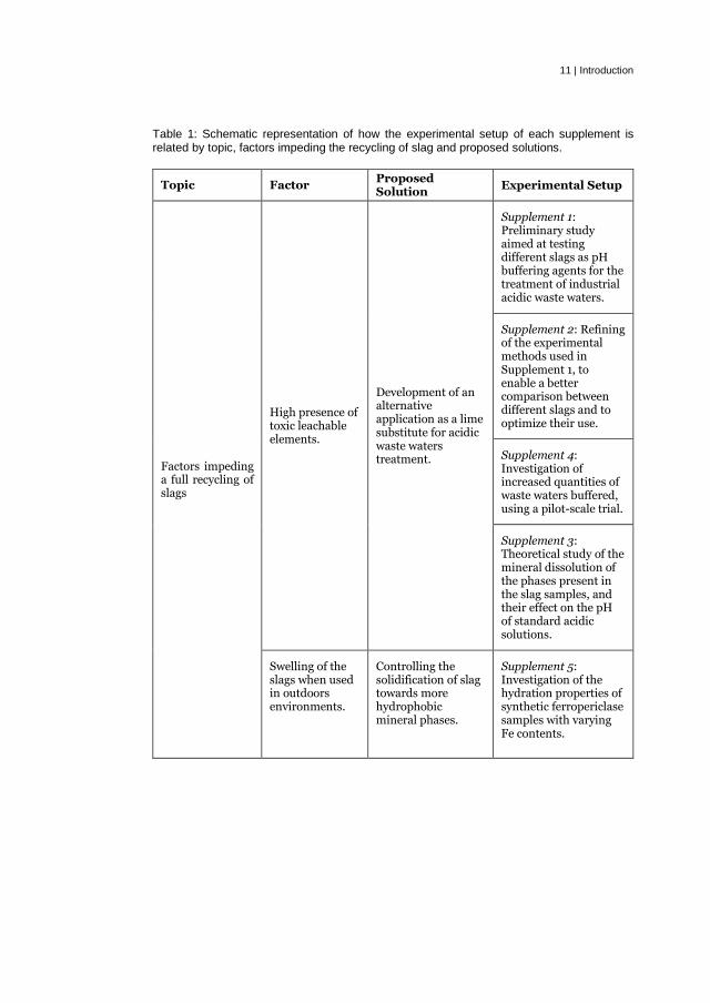
Table 1: Schematic representation of how the experimental setup of each supplement is related by topic, factors impeding the recycling of slag and proposed solutions.

Topic Factor Proposed Solution

Experimental Setup

Factors impeding a full recycling of slags

High presence of toxic leachable elements.

Development of an alternative application as a lime substitute for acidic waste waters treatment.

Supplement 1: Preliminary study aimed at testing different slags as pH buffering agents for the treatment of industrial acidic waste waters.

Supplement 2: Refining of the experimental methods used in Supplement 1, to enable a better comparison between different slags and to optimize their use.

Supplement 4: Investigation of increased quantities of waste waters buffered, using a pilot-scale trial.

Supplement 3: Theoretical study of the mineral dissolution of the phases present in the slag samples, and their effect on the pH of standard acidic solutions.

Swelling of the slags when used in outdoors environments.

Controlling the solidification of slag towards more hydrophobic mineral phases.

Supplement 5: Investigation of the hydration properties of synthetic ferropericlase samples with varying Fe contents.

Introduction | 12

13 | Experimental Methods

2. Experimental Methods

The present chapter gathers all the experimental methods used in this

thesis. Since supplements from 1 to 4 relate to the same topic of

investigation, the methods used in the different studies are grouped

together to highlight differences and similarities developed over time. On

the other hand, the experimental methods utilized in Supplement 5 are

described in a separate subchapter, as they are not the same used in the

other supplements.

This chapter aim at providing only a summary of the methods used, while

the supplements will provide a more thorough explanation of all the

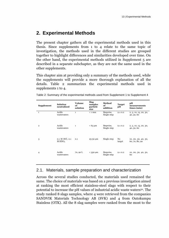
details. Table 2 summarizes the experimental methods used in

supplements 1 to 4.

Table 2: Summary of the experimental methods used from Supplement 1 to Supplement 4

Supplement Solution neutralized

Volume of solution

Slag samples particle size

Method of addition

Target pH

pH measurements times (min)

1 Acidic wastewaters

1 < 1 mm Stepwise, Single-step

9 ± 0.2 2, 5, 10, 15, 20, 30, 40, 50, 60


1 < 63 µm Stepwise, Single-step

9 ± 0.2 2, 5, 10, 15, 20, 30, 40, 50, 60

3 0.1 M HCl, 0.1 M HNO3

0.1 25-50 µm Single-step No target

10, 20, 30, 40, 50, 60, 70, 80, 90


70, 90 L < 350 µm Stepwise, Single-step

9 ± 0.2 10, 20, 30, 40, 50, 60

2.1. Materials, sample preparation and characterization

Across the several studies conducted, the materials used remained the

same. The choice of materials was based on a previous investigation aimed

at ranking the most efficient stainless-steel slags with respect to their

potential to increase the pH values of industrial acidic waste waters50. The

study ranked 8 slags samples, where 4 were retrieved from the companies

SANDVIK Materials Technology AB (SVK) and 4 from Outokumpu

Stainless (OTK). All the 8 slag samples were ranked from the most to the

Experimental Methods | 14

least efficient (lower g/L ratio needed to neutralize the pH of the

wastewaters). Thereafter, the best two performing slags from each

company were selected as materials to be used in this thesis. The material

code and the description of the slag samples is provided in Table 3. The

material code has been changed in this thesis and in all supplements expect

for in Supplement 2, that retained the code used in previous

investigations50. The slags samples have been taken from the same batch,

whenever possible, to provide an easier comparison between the different

studies. In fact, supplements 1, 2 and 3 use the same materials coming from

the same batch. Supplement 4 on the other hand, utilizes the same slag

type O1 but from a different batch compared to other studies, due to the

high amount of slag used in those tests. In addition, the same standard

grade lime powders have been used in several trials to provide a

comparison when the material was substituted with slag.

Table 3: Material code and description of the slag samples used in the pH buffering studies

Old material code Current material code Description

O3 O1 OTK Landfill slag

O1 O2 EAF slag

S4 S1 SVK Landfill slag

S1 S2 AOD slag

The sample preparation also varies across different studies. Due to the

heterogeneous nature of the materials used, several operations have been

conducted in Supplement 1 to produce slag powders that could be used in

the experiments. Slag samples O1 and S1, were already retrieved as fine

powders although the materials were quite wet, due to being stored in

outdoors landfills. On the other hand, slag samples O2 and S2 solidified in

big aggregates that needed to be crushed, but they were overall dry.

Therefore, the landfill slags were dried at 100°C for 24 h with no crushing,

whereas the EAF and AOD slags were crushed in three steps, by a jaw

crusher first, a spider crusher and finally by a horizontal shaft impactor.

After crushing and/or drying, both crushed and uncrushed samples were

sieved through a 1 mm mesh. Thereafter, PSD determinations were


conducted by using laser diffraction in an air media to characterize the

powders. In Supplement 2, the PSD was reduced even more, by ball-milling

all the slag samples and sieving them through a 63 µm mesh. In

Supplement 3, the samples that were ball-milled in Supplement 2 were

further sifted through several meshes and the interval 25-50 µm was

selected for the experiments. In Supplement 4 only slag sample O1 was

used. In this case, the slag sample was dried for 24 h at 105°C and sieved

through a mesh of 350 µm.

The mineral and chemical compositions of the slag samples were assessed

in Supplement 3. Semi-quantitative analysis of the mineral phases present

within each slag was performed using scanning electron microscope (SEM)

and X-ray powder diffraction (XRD), while the bulk chemical composition

was identified by using inductively coupled plasma (ICP) analysis after an

acid digestion.

During the experiments different acidic solutions were used. In

Supplements 1 and 2, the rinsing waters derived from the pickling process

that are commonly treated in the neutralization plants of OTK and SVK,

were sampled and used for the experiments. The waste waters were stored

in several buckets having volumes of 20-30 L each. Usually, a mixture of

several acids is used depending on the steel grade and the specific process

at the company. Thus, the composition across several buckets could not be

maintained the same. Therefore, the pH level varied, but it always ranged

between the values 1 and 2. In addition, only slags and waste waters from

the same company were tested together. In Supplement 4, the focus was

pilot-scale trials. Given the large quantity of wastewaters to treat, they were

extracted with a pump directly from the tanks where they were stored

during the industrial processes in OTK. Therefore, the composition was

also not controlled during all the experiments. In Supplement 3, the waste

waters were substituted by laboratory made acidic solutions. Two 0.1 M

(pH 1) HCl and HNO3 solutions were created by mixing standard grade

chemicals with distilled water. The solutions were used to provide a more

reliable comparison between slags samples, as the goal of the

investigations was to address the different solubilities of slag minerals, as

well as their effect on the pH of the solutions being used.

2.2. pH Buffering Trials

The pH buffering trials are the main focus of this thesis, as the aim was to

develop a new application for stainless-steel slags, substituting lime for the

treatment of acidic waste waters. The pH buffering methods were


developed in Supplement 1, and were kept constant across several sets of

experiments with only some minor variations, depending on the specific

case examined.

2.2.1. Stepwise dosing method

The single stepwise dosing method was developed as a preliminary

investigation that could approximately determine the correct range of slag

weight to use, avoid excessive consumption of materials. In fact, since the

single-step dosing method is a trial-and-error procedure that needs to be

repeated until the right quantity of slag is found, it can be prone to

materials and time waste. The stepwise dosing method consists of

dropping an arbitrary small quantity of slag in the waste waters, either in

a liquid solution or in powder form, until a stable pH value is reached. The

procedure is repeated until the target value pH of 9.0 ± 0.2 is reached. Once

the final pH value is obtained, the total amount of slag used is summed up.

The pH value of 9 was chosen, in collaboration with the industrial partners,

as the minimum value to reach, since it roughly mimics the pH values

obtained during their treatment processes, which over around 11. In

addition, before inserting a new slag quantity, the experiments needed to

define a definition for what can be considered a stable value of pH. In fact,

the dissolution of the slag minerals occurs over several hours, but the main

contribution is in the early stages after the weight is dropped into the acidic

solution. Therefore, it was arbitrary chosen that to determine a stable value

of pH, the rate of increase of the pH should not exceed a variation of 0.3

after 10 min from the last measurement. Specifically, assuming an

arbitrary small quantity of slag is poured in the acidic solution at t = x min,

the pH value is measured at t = x+10 min and subsequently at t = x+ 20

min. If |pHx+20 – pHx+10| ≤ 0.3 and lower than 9.0 ± 0.2, a new quantity of

slag is inserted. If the first condition is not met, a third measurement

occurs at t=x+30 min or until the pH stabilizes, according to the previous

definition. When the pH value reaches 9.0 ± 0.2 the trial is stopped, and

no more slag is dropped into the acidic solution. During the stepwise

dosing method, no limit of time is imposed, and the length of the trial is

determined uniquely by the numbers of iterations performed. The total

amount of slag poured during the trial is then used as a benchmark for the

single single-step dosing method. A schematic representation of how the

pH values increase over time as a result of several slag additions, is shown

in Figure 2. The stepwise dosing method has been used in Supplements 1,

2 and 4. In the first two, the quantity of waste waters used was 1 liter, while

in the third a tank filled with 70 and 90 liters was used.


Figure 2: A schematic representation of a stepwise dosing trial with three additions of reactant

In Supplement 1, 10 trials were conducted using this procedure. Both lime

products from OTK and SVK along with the four slag samples from these

companies were tested. Duplicates were performed for the sample that

neutralized the waste waters the first time. In Supplement 2, each of the

materials used in Supplement 1 were tested once. Thereafter, their results

were compared to the precedent trials. In Supplement 4, the method was

used once again to determine the range of slag quantities to use when the

volumes were upscaled to volumes of 70 L and 90 L. Three trials were

conducted, all of them using slag O1. Two using 90 L of waste waters and

one using 70 L. In Supplement 3, the method has not been used since the

quantities of slag to insert were fixed.

2.2.2. Single-step dosing method

Contrary to the stepwise dosing one, the single-step dosing method was

developed to mimic, as closely as possible, the industrial conditions of the

wastewater’s treatment processes used at OTK and SVK. There, lime is

poured as a single addition to the volume of waste waters, with occasional

further additions if the quantity inserted does not increase the pH values

to the desired targets. Therefore, a method like the stepwise dosing method

is unfit to provide valuable information to the companies, with the respect

to the possibility of substituting lime with slag in their processes. However,


also the single-step dosing method present a limitation being a batch test.

In fact, the industrial processes operate in a condition of constant flow,

with different kinetic conditions than a beaker or tank agitated by a stirring

mechanism. Nonetheless, since a continuous flow could not be replicated,

a time limit of 30 min was set as an approximation of how much time is

spent by the waste waters in the neutralization process, before the mass of

liquid reaches the flocculation and sedimentation phase. Compared to the

previous method, the pH target of 9.0 ± 0.2 was maintained the same, but

a time condition was added. For the single-step dosing trials the optimal

quantity of slag was defined as the one that reaches a pH value of 9.0 ± 0.2

within 30 minutes after the slag injection.

Contrary to the stepwise dosing method, a single addition of slag, which

amount has been calibrated based on the results of the stepwise dosing

methodology, is selected to be dropped at t = 0 min. Then, the pH values

are measured at different intervals for 60 min (in Supplement 3 the time is

extended at 90 min). The times when the pH values are measured varied

depending on the experiments performed. In Supplement 1 the time

intervals were set at t=2/5/10/15/20/30/40/50/60 min, whereas in

Supplement 2 the measurement at minute 2 was eliminated. In

Supplement 3 and 4 also the measurement at minutes 5 and 15 were also

eliminated.

Also, the method of addition of the reactant changed over the course of the

different experiments. In Supplement 1 the quantity of slag chosen was

mixed with distilled water, forming a 40 wt% reactant suspension to be

poured in the waste waters. From Supplement 2 on, the slag was dropped

directly as a powder inside the waste waters. The change was made since it

did not influence the results of the trials and the new method was easier

and more precise. Another variation was introduced in Supplement 3. In

fact, since the goal of the study was to understand the different dissolution

rates of the slag minerals, trials with fixed mass were preferred to the ones

with a pH target value. All slag samples were tested by using fixed

quantities of 0.5, 1, 2 g apart from slag sample S2 were only quantities of 1

and 2 g were used. Therefore, contrary to previous experiment, the

investigation focused on comparing the different pH values reached by

using the same quantity of different slags, rather than aiming at reaching

the same pH value and comparing the different weights to do so.

The quantity of waste waters used in the single-step dosing trials changed

between sets of experiments. In Supplements 1 and 2, 1L beakers were used

to contain the waste waters. In Supplement 4, tanks filled with 70 and 90L


of waste waters were used instead, while in Supplement 3 beakers

containing 100ml of 0.1 M HCl/HNO3 solutions were used. A schematic

representation of how the pH increases over time, corresponding to a

single slag addition, is shown in Figure 3.

Figure 3: A schematic representation of a single-step dosing trial with one addition of reactant.

Finally, not all the slags were tested with all the methods across the

different supplements. In Supplement 1, all the reactants that could bring

the pH to the target value using the stepwise dosing trials were used as well

for the single-step dosing trials. Therefore, only slag samples O1, S1 and

two lime products were tested with the single-step dosing method to find

the optimal quantity that could yield the target pH value. In Supplement 2,

slag samples O2 and S2, which previously did not rise the pH to the target

value during the stepwise dosing method, were successfully employed in

replicated experiments. Thus, the same sample samples had been tested

using the single-step dosing methodology as well. Furthermore, only slag

sample O1 has been employed in stepwise and single-step dosing trials in

Supplement 4, with volumes of 70 and 90L. Finally, in Supplement 3, 19

trials were conducted using different slag types, slag weights and acidic

environments depending on the scope of the investigation.

2.2.3. Concentration of toxic elements

The treatment processes in OTK and SVK aim not only to increase the pH

of the wastewaters, but also to remove traces of metallic elements dissolved

in them, before they can be poured in the regular water streams. Metallic


elements such Cr, Ni, Fe, Mo, and Zn are present in the industrial waste

waters and slags needs to absorb them equally well compared to lime, to be

used as an efficient substitute. Therefore, additional single-step trials were

performed using slag O1 to neutralize the OTK industrial acidic waste

waters. The trials were also conducted using lime with the same setup to

provide a comparison. Flocculants were used to facilitate the collection of

the solid particles and paper filters were used to separate them from the

liquid. Finally, the compositions of the treated and filtered industrial waste

waters samples were determined using ICP-MS, to determine the

concentrations of Cr, Ni, Fe, Mo and Zn. The concentrations of metallic

elements obtained with lime and the ones obtained with slag were

compared to each other. They were also compared to the threshold limits

imposed by the Swedish law.

2.2.4. Analysis of the solid residues

In Supplement 3 analyses of the residues obtained after the pH buffering

of standard 0.1 M HCl/HNO3 solutions are performed, both by using slag

and standard lime products. To do so, the beakers of the neutralized acidic

solutions were put in a ventilated oven at 90°C overnight, so that the liquid

phase could evaporate without boiling. Afterwards, the powders remaining

in the beakers were removed, ground with a mortar, and dried again in the

oven at 105°C for 30 min to eliminate all remaining moisture. The dried

powders were then ground again in a mortar. Thereafter, XRD analyses

were performed on all the samples extracted with this method. In addition,

SEM coupled with energy-dispersive X-ray spectroscopy (SEM-EDS)

analyses were used to determine the chemical compositions of the

powders, when the XRD analyses were not sufficient.

2.3. Pilot-scale Trials

To promote the use of slag as lime substitute for the treatment of acidic

waste waters, pilot-scale trials were performed by upscaling the volumes

tested in previous supplement. From a 1 L volume tested in Supplements 1

and 2, the goal in Supplement 4 was to up-scale the experiments to volumes

of 70 and 90 liters. To do so, a physical model was developed to determine

the mixing conditions that would fit with the scope of the investigation. The

objectives of the physical model trials were two. First, to determine a set of

parameters that, when varying the volume of waste waters tested, would

maintain comparable mixing conditions of trials when using different

volumes. Thereby, the amount of slag used to neutralize the waste waters

would be dependent on the increase on the volume only. Moreover, the


mixing conditions needed to guarantee a fast spread of the slag in the

volume, so that the pH level across the whole volume could be

homogenized as fast as possible, especially by the time when the first pH

measurements occurred, namely after 10 minutes from the start of the trial.

The mixing conditions were firstly tested with the use of a physical model.

A tank was filled with water containing the following volumes: 70, 80 and

90 L. An impeller was used as the stirring mechanism, and it was placed

along with an overhead engine, on top of a steel frame on surrounding the

tank. To simulate the dispersion of slag in the water, 20 ml of a 20 wt%

NaCl solution was added as a tracer. Meanwhile, conductivity probes were

used to measure the conductivity of the solution over time. This is a

common setup used in several reported studies, mostly to determine the

mixing conditions of AOD converters 51–60. To quantify the time when the

tracer is homogenously distributed inside the tank, a parameter called

mixing time (Tm) is defined. Specifically, Tm is the time after which the

conductivity of the solution Ci always satisfies the following condition:

Ci

Cfinal

=1 ±0.05 (1)

Figure 4 shows a graphical example of how Tm can be calculated by using

the conductivity values measured by the probe. Tm is the time after which

the Ci/Cfinal ratio stabilizes within the range of 1.00 ±0.05. In case of

multiple probes, as used in for the current setup, Tm is calculated by taking

the higher value among the mixing times calculated for each probe.


Figure 4: Graphical example of how mixing time can be calculated given the ratio Ci/Cfinal over time.

This parameter was used to determine the variation of the mixing

conditions when several parameters are changed. The goal was to obtain

the same mixing condition. Thus, approximately the same Tm values when

70 and 90 L of waters were stirred. To do so, 30 trials were conducted,

where the conductivity probe positions, the volume of water where the

tracer was inserted where changed. Furthermore, the stirring speed

provided by the impeller. A detailed list of all the parameters used can be

found in Supplement 4. First, the parameters that could ensure a similar

mixing condition between the 70 and the 90 L trials were determined.

Thereafter, the pilot-scale trials were continued using the stepwise and

single-step dosing methods.

2.4. Hydration of ferropericlase

This last subchapter describes the experimental methods used in the

standalone project regarding the hydration of FP. These experiments

cannot be summarized with the ones performed throughout Supplements

1 to 4, as Supplement 5 used an entirely different set of experimental

methods compared to the others.

2.4.1. Materials, sample preparation and characterization

To synthetize FP, the study largely relied on the methods and procedures

developed by the field of geology, where the minerals have been abundantly


studied61–65. Although the structure of FP is hard to evaluate and control,

because it contains both trivalent iron (Fe3+) and bivalent iron (Fe2+), and

the ratio between the two is affected by parameters such temperature,

pressure and oxygen fugacity66. Although, many suitable options are

available to prepare synthetic samples of FP67. This study focused on solid-

solid reactions (i.e sintering). In the literature analyzed, the material used

to prepare the FP samples were MgO and iron oxides (Fe2O3 or FeO)

powders, which have been sintered at temperatures between 1473 and 1873

K for more than 12 h49,61,62,67–70. Moreover, the powders were sintered with

the use of a mixture of CO and CO2 or other inert gases49,67,69. In fact,

decreasing the oxygen partial pressure reduces the formation of Fe3+ in the

FP matrix, while impeding the exsolution of a phase having a composition

(Fe,Mg)Fe2O461,68.

The FP samples were prepared starting from FeO and MgO powders. The

weights have been carefully measured to produce samples containing 0,

90, 85 and 80 wt% of MgO (labeled as “MgO”, “10 wt% FeO”, “15 wt% FeO”

and “20 wt% FeO”). Specifically, the real FeO wt% values of each sample

were 0, 10.20, 15.01 and 21.71, respectively. The powders were firstly mixed

in a mortar and then pelletized. The pellets were then sintered in furnace a

1773 K for 24 h in an Ar atmosphere. The oxygen partial pressure was

estimated to have a value of approximately 10-6 atm71. Thereafter, the

samples were cooled at a rate of 300 K/h. After the first round of sintering,

the pellets were removed. Successively, they were crushed into a powder,

ground in a mortar, re-pelletized and sintered again using the same

parameters. Finally, the pellets were cut longitudinally in half and their

internal surfaces were examined by using an Electron Probe Micro

Analyzer (EPMA). The remaining parts of the samples were crushed into

powders and ground in a mortar. Subsequently, XRD analysis, Mössbauer

spectroscopy and PSD analysis were conducted to evaluate the phase

composition, Fe oxidation state, and particle size distribution, respectively.

2.4.2. Hydration method design

The following step of the study was to develop a reliable hydration method.

The primary objective was to provide a complete hydration of the powders,

meaning that the water absorption needed to be as close as possible to the

theoretical maximum one. Since the amount of water adsorbed by FP is

unknown, MgO was used as a reference material to develop the hydration

method. A chemical model was developed using ideal chemical formulas

and reference values of molar weights. Then, thermogravimetric analysis

(TGA) determinations were performed on an industrial-grade brucite


powder sample. Using an Ar atmosphere, the trial was started by recording

the mass change from 40 °C on, using a heating rate of 15 °C/min up to the

final temperature of 800 °C. Thereafter, the temperature was kept constant

for 20 min before finishing the trial. The dehydration of brucite was

compared to the chemical model predictions, to evaluate if TGA was a

suitable method to determine the amount of water released during the

dehydration of the mineral. Autoclave curing was then utilized to hydrate

MgO powers to form brucite. Thereafter, TGA was performed on the

hydrated MgO samples. The results were compared to the dehydration of

industrial brucite, to determine whether the parameters chosen could

provide a complete hydration of MgO. Autoclave curing is a standard

process used in the cement industry to simulation the hydration of

cements, but it is also used to simulate the weathering of steelmaking

slags72–77. The MgO powders were mixed with different ratios of water and

then heated to a constant temperature of 120°C for 24h. The internal vapor

pressure was estimated to be 2 atm75. The powders were dried in a

ventilated oven for 18 h at 105 °C. Finally, TGA determinations were

conducted on the hydrated MgO powders. The same parameters used for

the dehydration of brucite were selected once again.

2.4.3. Hydration of ferropericlase, TGA analysis and characterization

All FP samples were cured in an autoclave by using the same procedure as

used as for the MgO powders. Compared to the trials performed with MgO,

the ratio between the FP powders and water was fixed to 0.4 g and 5 g,

respectively. Three hydrated batches of each FP sample were produced.

Also, TGA was performed as the dehydration of both brucite and hydrated

MgO powders. The TGA determinations were performed on each batch of

each hydrated sample for a total of 9 trials. Thereafter, a final

characterization using XRD was performed.

25 | Results

3. Results

3.1. Material characterization

3.1.1. Mineral and chemical composition

Semi-quantitative analyses were conducted to determine the mineral

compositions of the four slag samples used throughout all the pH buffering

experiments. The analyses were conducted by combining both XRD and

SEM spectroscopy’s studies performed on the samples. Figure 5

summarizes the mineral phases present in each sample and their contents

expressed in percentage. The results are based on the use of a semi-

quantitative method, which compares the intensity peaks of each phase in

the XRD spectrum and uses SEM to identify the minerals present in the

samples. Therefore, the results are meant to serve as a guideline, rather

than being a precise value describing the slag mineral compositions.

Nonetheless, the results are quite informative and can be used to make

some useful comparisons between the slag samples. A more detailed list of

the minerals, with chemical formulas and crystal system are found in Table

4.

Figure 5: Semi-quantitative analysis of the mineral phases, expressed as % of the total, of the four slag samples O1, S1, O2 and S2.

Results | 26

Table 4: Compound name, chemical formula and crystal system of each mineral found in the slag samples

Compound Name Chemical Formula Crystal System

dicalcium silicate γ Ca2 O4 Si1 Orthorhombic

bredigite (O1) Ca26.93 Ba0.59 Mg3.62 Mn0.86 Si16.00 O64.00

Orthorhombic

bredigite (S1) Ba0.3 Ca13.5 Mg1.8 Mn0.4 O32 Si9 Orthorhombic

fluorite Ca1 F2 Cubic

magnesiochromite (O1) Mg6.96 Fe1.04 Cr16.00 O32.00 Cubic

magnesiochromite (O2) Cr2 Mg1 O4 Tetragonal

magnesiochromite (S1) Al7.78 Fe3.59 Mg4.70 Mn0.05 Si0.01 Zn0.05 Cr7.78 Ni0.01 Ti0.02 O32.00

Cubic

åkermanite (O1) Ca4.00 Mg1.42 Al1.02 Si3.48 O14.00 Tetragonal

åkermanite (S1) Ca4.00 Mg0.92 Al1.98 Si3.04 O14.00 Tetragonal

cuspidine Ca16.00 Si8.00 O28.00 F8.00 Monoclinic

merwinite Ca3 Mg1 O8 Si2 Monoclinic

dolomite Ca3.00 Mg3.00 C6.00 O18.00 Hexagonal

periclase Mg1 O1 Cubic

portlandite H2 Ca1 O2 Hexagonal

magnesioferrite Mg8.00 Fe16.00 O32.00 Cubic

mayenite Al14 Ca12 O33 Cubic

Slag sample S1 is the most complex system among the four studied. In fact,

it contains 6 mineral phases with contents higher than 1%. Conversely, slag

sample S2 is the simplest one, being made up of a binary system consisting

of dicalcium silicate γ and mayenite. The slag samples O1 and O2 both

contain 4 mineral phases each having contents of more than 1% in

concentration. There are also some recurrent phases present in the slag

samples: dicalcium silicate γ, åkermanite and bredigite which are present

in at least 3 samples. These minerals are very common in metallurgical

slags and their presence have been reported in several studies1,4,5,17,78–80.

The bulk chemical compositions of the slag samples were also determined.

Since elements such as Si, Ca and Mg react in aqueous media, altering the

pH of the solutions where they are dissolved 81,82, the total amounts of these

elements was measured using ICP spectroscopy. Figure 6 presents the five

most abundant elements for each slag sample, among the 32 tested using

ICP (the full list is presented in Supplement 3). As seen, Ca is the most

abundant element, which roughly constitutes 30 wt% of all samples.

27 | Results

Except for slag S2, Si is the second most abundant element, which content

is higher than 10 wt% in each sample. Furthermore, Mg is the third most

common element with contents ranging from 4 to 7 wt%. Al is the fourth

most abundant in slags O1 and O2, whereas it is the second most common

element in the slag S2 and the fourth in slag S1. The remaining elements

are Cr, Mn and Fe which contents range from 3 to 1 wt%. The remaining

roughly 50% of each sample is made by oxygen.

Figure 6: Amount in wt% of the most abundant elements of all the slag samples

3.1.2. Particle size distribution

After slags S2 and O2 were crushed, the distributions of the particle sizes

of all slags were analyzed and the results were compared to each other. In

addition, the particle size of the lime powders used in the pH buffering

trials were also determined and the results were compared to the particle

size distributions of the slag samples. As is it possible to notice from Figure

7, the PSDs of the various samples differ. The O2 and S2 powders are the

coarsest, since they were not retrieved already in a powder form. They have

similar D50 and D90 values (meaning the diameters under which 50 and 90

% of the value is contained): 219 and 557 µm for slag O2 and 196 and 542

µm for slag S2. The only difference between these samples is the presence

of higher amounts of finer particles in slag O2 compared to slag S2.

0% 10% 20% 30% 40% 50% 60%

S2

O2

S1

O1

Ca Si Mg Al Fe Mn Cr

Results | 28

Specifically, this is represented by a smaller D10 value of 17.6 µm compared

to a value of 53.0 µm. Slag S1 has a similar D10 value to slag O1 (12.6 µm),

but it also has roughly a third of its D50 value (72.5 µm) and half of its D90

value (261 µm). This is also visible from the particle size distribution shown

in Figure 7. Moreover, compared to slags O2 and S2, slag S1 presents a finer

distribution of particles. In addition, slag O1 has a more spread distribution

of particle sizes. In fact, compared to the other slags, it has the lowest D10

and D50 values (4.18 µm and 32.8 μm, respectively) but a comparable D90

value to slags O2 and S2 (521 μm). Therefore, it is harder to classify slag O1

compared to the other samples. On the contrary, the lime samples are

clearly the finest powders, having D90 values of 50.9 and 39.1 for OTK lime

and SVK lime, respectively.

Figure 7: PSD of the slag samples after being crushed and sieved through 1 mm mesh

3.2. Laboratory stepwise dosing method experiments with

acidic waste waters

The results of the experiments performed with the stepwise dosing method

related to Supplement 1 (<1 mm) and Supplement 2 (<63 μm) are

compounded in Table 5. The methodology was first applied once to all slag

samples with PSD <1 mm. In the first set of trials, only slags S1 and O1

could successfully rise the pH to the target values (9.0 ± 0.2). The trials

0

10

20

30

40

50

60

70

80

90

100

0.1 1 10 100 1000 10000

cum

ula

tiv

e volu

me

(%)

particle size (µm)

O1

O2

S1

S2

Lime OTK

Lime SVK

29 | Results

using slags O2 and S2 were interrupted, since high weights (more than 30

g/L) of the materials could not significantly rise the pH value of the

solution tested. Successively, replicates of the trials were performed using

slags O1 and S1. In the retrial, slag O1 was overdosed, so that a pH value

higher than the target is reached, whereas slag S1 successively reached the

target value once again. Despite the differences in the weights obtained in

the retrial with O1, the results seemed comparable given the differences in

pH values. On the other hand, the slag S1 trial rose the pH to almost the

same values given a very similar weight.

In a subsequent set of trials, the particle size distribution of the powders

was reduced by first ball-milling the samples and then sieving them

through a mesh of a 63 μm size. The weight needed to reach the target pH

values dropped by 35-40% for slags O1 and S1. This, in turn, visibly reduced

the quantity of slag needed to perform the pH buffering of the acidic waste

waters. A similar effect happened when using slags S2 and O2. However,

the first set of trials could not be completed so that no estimation of the

reduction of the weight could be calculated. Nonetheless, contrary to

previous trials, the materials (< 63 µm) successfully reached the target pH

value imposed by the experiments. Slag S2 was overdosed during the trial,

meaning the quantity to reach the target value of pH is lower than the one

showed in Table 5.

Table 5: Stepwise dosing method applied with powders sifted through a mesh of 1mm and 63µm. Successful trials conducted with powders <1mm were replicated once more (slag O1 and S1).

Slag O1 O2 S1 S2

PSD (µm)

< 1000 < 63 < 1000 < 63 < 1000 < 63 < 1000 < 63

weight (g/L)

22.8 28.6 14.7 32.2 23.5 23.6 23.3 14.6 36.3 25.2

pHfinal 9.1 9.4 9.2 5.8 9.1 9.1 9.0 9.2 5.3 10.0

Results | 30

3.3. Laboratory single-step dosing method experiments using

acidic waste waters

The results of the single-step dosing method are the focus of the pH

buffering trials. In fact, this method of slag addition is the one that more

realistically resembles the industrial processes. Thus, it provides a more

insightful information regarding the use of stainless-steel slags for the

treatment of acidic waste waters at industrial conditions. In Figure 8, the

results of six single-step dosing method trials conducted using slag samples

O1 and S1 with PSD < 1mm are reported. For each slag, three trials are

shown. To consider the trial successful, the pH value at the 30th minute

after the beginning of the trial had to be equal to 9.0 ± 0.2. Therefore, for

slag O1, only the one with a 39 g addition was able to reach the desired

target value (pH30=9.1). On the other hand, in case of slag S1, the trials

using 48 g and 49 g additions were both able to reach the correct pH value

by minute 30 (pH30=9.1 and 9.0 respectively). When comparing successful

and unsuccessful trials, some additional considerations can be drawn. All

the six trials present the same trend: there’s a sudden surge of the pH

values when slag is inserted in the batch of acidic waste waters. Thereafter,

the increase rate quickly diminishes during the first 5-10 minutes of the

trial. Successively, the pH value either remains mostly stable or it slowly

increases, until a second (smaller) surge appears. This is more visible when

using slag O1, where the pH value remains mostly stable, compared to slag

S1 that still shows an increase before the second surge. Noticeably, the time

when the second surge happens appears to be dependent on the inserted

slag weight. In fact, in all six trials, the higher the weight of slag used, the

quicker the second rise in pH value appears.

A consequence of the delayed appearance of the second surge in pH value

is that the differences in pH levels between the trials diminish with time.

This is possible to notice by analyzing the pH values at minutes 30 and 60

of the different trials. In case of slag O1, the difference in pH value at

minute 30 between the 39.0 g trial and the 33.9 g trial was 0.7. Compared

to the 28.5 g trial it was 2.5. At minutes 60, the differences are 0.3 and 1.1,

respectively. The same is true for slag S1. At minute 30 the difference in pH

levels between the 48.0 g trial and the 38.9 g trial was 2.0, but only 0.7 by

the end of the trial.

31 | Results

Figure 8: Laboratory single-step trials with slag sample O1 and S1 sieved through a 1 mm mesh

Trials with standard grade lime products were also conducted to compare

the performance of the slag sample with the current reactant used to

neutralize the acidic waste waters. As it is noticeable from Figure 9, the use

of lime makes it possible to reach the final pH value before even the first

measurement (5.9 g of lime SVK or 4.9 g of lime OTK) or by minute 10/15

when the weight is lower.

Figure 9: Laboratory single-step trials with lime samples from OTK and SVK

Additional single-step dosing trials were conducted using slag samples O1

and S1 with a reduced PSD to < 63 µm. Contrary to precedent trials, slag

O2 was successively employed in stepwise dosing trials. Therefore, it could

be employed in single-step trials too. Slag S2 also successively buffered the

pH values in the stepwise trials. However, during the single-step trials the

slag particles were partially deposited on the bottom, forming a hard crust

on the beakers’ walls, rather than forming a suspension within the acidic

bath. This unexpected chemical reaction forced an interruption of the

Results | 32

trials. Nonetheless, Figure 10 shows the single-step trials conducted using

the remaining slag samples.

Figure 10: Laboratory single-step trials with slag sample O1, S1 and O2 after ball-milling and sieving through a 63 µm mesh

As for the stepwise trials, the reduced PSD value also reduces the weight of

slag used to reach the target pH value. The reduction is increased

compared to the stepwise trials, namely from 35-40% to 50%. In fact, slag

O1 buffered the pH to the target value when using a 20 g addition, while

slag S1 needed a 23 g addition to reach the target value. This is roughly half

the amount used in trials with slags with coarser particles size

distributions, which needed additions of 39 g and 49 g, respectively. No

precedent comparison exists for slag O2. However, compared to the other

slags, it reaches the pH target value by using roughly double their weight

(39.0 g). Furthermore, despite the reduction in PSD, the curves of the pH

values over time resemble the ones produced in the precedent single-step

trials. Similar to what was found in previous experiments, there is a rapid

surge in the pH value followed by a plateau that ends with a second surge.

This is more visible in the trials using lower amounts of slag, as this effect

starts to disappear when the weight of slag increases. Specifically, this is

observed for the trial using 25.0 g addition of slag O1. It appears that for

all slag samples the second surge of pH is pushed towards the beginning of

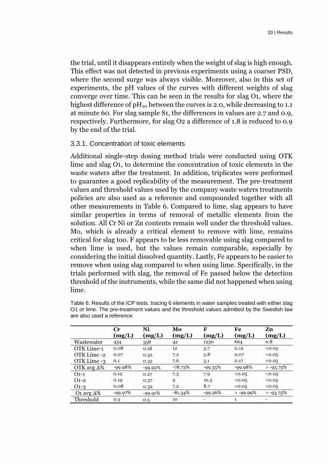
33 | Results

the trial, until it disappears entirely when the weight of slag is high enough.

This effect was not detected in previous experiments using a coarser PSD,

where the second surge was always visible. Moreover, also in this set of

experiments, the pH values of the curves with different weights of slag

converge over time. This can be seen in the results for slag O1, where the

highest difference of pH30 between the curves is 2.0, while decreasing to 1.1

at minute 60. For slag sample S1, the differences in values are 2.7 and 0.9,

respectively. Furthermore, for slag O2 a difference of 1.8 is reduced to 0.9

by the end of the trial.


Additional single-step dosing method trials were conducted using OTK

lime and slag O1, to determine the concentration of toxic elements in the

waste waters after the treatment. In addition, triplicates were performed

to guarantee a good replicability of the measurement. The pre-treatment

values and threshold values used by the company waste waters treatments

policies are also used as a reference and compounded together with all

other measurements in Table 6. Compared to lime, slag appears to have

similar properties in terms of removal of metallic elements from the

solution. All Cr Ni or Zn contents remain well under the threshold values.

Mo, which is already a critical element to remove with lime, remains

critical for slag too. F appears to be less removable using slag compared to

when lime is used, but the values remain comparable, especially by

considering the initial dissolved quantity. Lastly, Fe appears to be easier to

remove when using slag compared to when using lime. Specifically, in the

trials performed with slag, the removal of Fe passed below the detection

threshold of the instruments, while the same did not happened when using

lime.

Table 6: Results of the ICP tests. tracing 6 elements in water samples treated with either slag O1 or lime. The pre-treatment values and the threshold values admitted by the Swedish law are also used a reference.

Cr (mg/L)

Ni (mg/L)

Mo (mg/L)

F (mg/L)

Fe (mg/L)

Zn (mg/L)

Wastewater 434 358 42 1230 664 0.8

OTK Lime-1 0.08 0.18 12 5.7 0.12 <0.05

OTK Lime -2 0.07 0.32 7.2 5.8 0.07 <0.05

OTK Lime -3 0.1 0.32 7.6 5.1 0.17 <0.05

OTK avg Δ% -99.98% -99.92% -78.73% -99.55% -99.98% > -93.75%

O1-1 0.12 0.27 7.3 7.9 <0.05 <0.05

O1-2 0.19 0.37 9 10.5 <0.05 <0.05

O1-3 0.08 0.32 7.2 8.7 <0.05 <0.05

O1 avg Δ% -99.97% -99.91% -81.34% -99.26% > -99.99% > -93.75%

Threshold 0.5 0.5 10 - 1 -

Results | 34

3.4. Laboratory single-step dosing method experiments with

standard acidic solutions

In Supplement 3, the focus of the single-step dosing method trials was to

determine the effect of the chemical and mineral composition in the ability

to buffer the pH levels of acidic solutions. To obtained more precise results,

the time and pH levels restrictions, that were used in the previous single-

step dosing experiments, were removed. Furthermore, for the same reason,

the acidic wastewaters used in previous trials were changed to standard 0.1

M HCl and HNO3 solutions. In addition, since the pH target value

condition was removed, trials with fixed weights of 0.5, 1 and 2 g were

conducted for each slag sample.

3.4.1. Effect of weight and composition

The results of the fixed weight single-step dosing method trials are

compounded in Figure 11. In all the trials, a 0.1 M HCl solution was used.

The trials are grouped based on slag sample, so the effect of weight for each

slag can be visible. For slag samples O1, S1 and O2, a 1 g addition was

sufficient to neutralize the pH value of the acidic solutions. On the other

hand, an addition of 0.5 g could not rise the pH to neutral values. When 2

g of slag are added, the pH value is increased compared to the trials with a

1 g addition. Specifically, the differences in the final pH value are 0.8, 0.9

and 1.4 for the slag samples O2, O1 and S1, respectively. In addition, when

looking at the curves of slag samples S1 and O2, it visible that the reaction

rate when using a 2 g addition is faster, since the difference of the final pH

values is lower than at the initial stages of the trial. In fact, after 10 minutes

after the start of the trial the difference in pH levels between the 1 g curve

and the 2 g curve is 3.6 for slag S1 and 2.9 for slag O2, compared to the pH

value difference beforementioned. However, for slag O1, the difference

remains constant around 1 point of pH for the whole length of the trial.

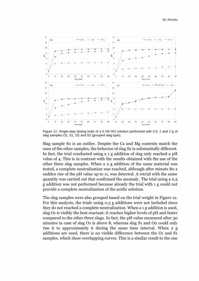
35 | Results

Figure 11: Single-step dosing trials of a 0.1M HCl solution performed with 0.5, 1 and 2 g of slag samples O1, S1, O2 and S2 (grouped slag type).

Slag sample S2 is an outlier. Despite the Ca and Mg contents match the

ones of the other samples, the behavior of slag S2 is substantially different.

In fact, the trial conducted using a 1 g addition of slag only reached a pH

value of 4. This is in contrast with the results obtained with the use of the

other three slag samples. When a 2 g addition of the same material was

tested, a complete neutralization was reached, although after minute 80 a

sudden rise of the pH value up to 11, was detected. A retrial with the same

quantity was carried out that confirmed the anomaly. The trial using a 0.5

g addition was not performed because already the trial with 1 g could not

provide a complete neutralization of the acidic solution.

The slag samples were also grouped based on the trial weight in Figure 12.

For this analysis, the trials using 0.5 g additions were not included since

they do not reached a complete neutralization. When a 1 g addition is used,

slag O1 is visibly the best reactant: it reaches higher levels of pH and faster

compared to the other three slags. In fact, the pH value measured after 30

minutes in case of slag O1 is above 8, whereas slag S1 and O2 could only

rise it to approximately 6 during the same time interval. When 2 g

additions are used, there is no visible difference between the O1 and S1

samples, which show overlapping curves. This is a similar result to the one

Results | 36

obtained during the single-step trials shown in Figure 10. Furthermore,

slag sample O2 reaches final pH levels of approximately 1.3 lower than the

other two slags (pH 9.6, 9.5 and 8.2 for samples O1, S1 and O2

respectively). As discussed before, a 1 g addition of slag S2 was insufficient

to provide a complete neutralization, contrary to the other samples.

However, a 2 g addition of slag provide a complete neutralization, while

also providing the highest pH values obtained in all the trials.

Figure 12: Single-step dosing trials of a 0.1M HCl solution performed with the slag samples S1, O1, O2 (grouped by added slag weight of 1g and 2g)

CaO was used as a reference in this set of experiments as well. As it is

possible to notice from Figure 13, a 0.25 g addition of CaO was insufficient

to neutralize the pH value of the acidic solution. Although the trial

conduced with a 0.5 g addition reaches a pH value of 12.5, which is the

value attributed to the dissolution limit of CaO83. Empirically this is also

shown by examining the content of the beaker. In the first case the solution

did not present any particulate, meaning that the CaO completely dissolved

in the acid. However, in the 0.5 g trial a suspension of lime powder could

be found. This is in line with chemical calculations performed considering

the chemical reactions between CaO and HCl, that shows that a 0.28 g

addition is a suitable quantity to bring the pH to neutral values. Therefore,

the ratio between slag and lime in this set of experiments to reach similar

pH values was found to be approximately 3.

37 | Results

Figure 13: Single-step dosing trials of a 0.1 M solution of HCl performed with 0.5g and 0.25g of CaO

3.4.2. Effect of acid environment

Four additional trials were conducted using 1 g additions of each slag, to

buffer the pH value of a solution of HNO3 with the same molarity as the

HCl one (0.1 M) previously used. The goal was to test whether the slag

samples had different solubilities in different acid environments. This can

be detected by plotting a different pH curve over time between the two

different solutions. Although, as noticeable from the results in Figure 14,

no meaningful variations in pH levels between the trials using two acids

were detected. In fact, the differences in measured pH values between the

two acidic solutions varied between 0.05 and 0.1 for slag samples O1, S1

and S2. For these materials, the HNO3 curves overlap almost perfectly with

the HCl ones. Only for slag O2 there was a slight difference of 0.7 between

the two final pH values. Regarding the remaining slags, the curve of the

test performed with HNO3 overlap almost perfectly with the HCl curves.

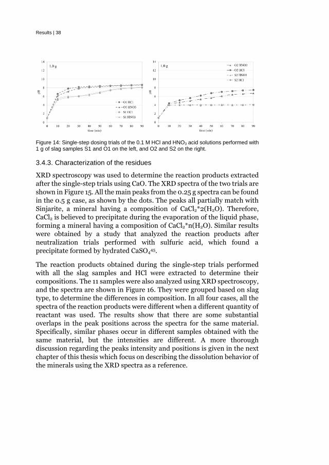
Results | 38

Figure 14: Single-step dosing trials of the 0.1 M HCl and HNO3 acid solutions performed with 1 g of slag samples S1 and O1 on the left, and O2 and S2 on the right.

3.4.3. Characterization of the residues

XRD spectroscopy was used to determine the reaction products extracted

after the single-step trials using CaO. The XRD spectra of the two trials are

shown in Figure 15. All the main peaks from the 0.25 g spectra can be found

in the 0.5 g case, as shown by the dots. The peaks all partially match with

Sinjarite, a mineral having a composition of CaCl2*2(H2O). Therefore,

CaCl2 is believed to precipitate during the evaporation of the liquid phase,

forming a mineral having a composition of CaCl2*n(H2O). Similar results

were obtained by a study that analyzed the reaction products after

neutralization trials performed with sulfuric acid, which found a

precipitate formed by hydrated CaSO445.

The reaction products obtained during the single-step trials performed

with all the slag samples and HCl were extracted to determine their

compositions. The 11 samples were also analyzed using XRD spectroscopy,

and the spectra are shown in Figure 16. They were grouped based on slag

type, to determine the differences in composition. In all four cases, all the

spectra of the reaction products were different when a different quantity of

reactant was used. The results show that there are some substantial

overlaps in the peak positions across the spectra for the same material.

Specifically, similar phases occur in different samples obtained with the

same material, but the intensities are different. A more thorough

discussion regarding the peaks intensity and positions is given in the next

chapter of this thesis which focus on describing the dissolution behavior of

the minerals using the XRD spectra as a reference.

39 | Results

Figure 15: XRD spectra of the residues extracted after the single-step trials of a 0.1M HCl solution performed with 0.25g and 0.5 g of CaO. The peaks related with the phase CaCl2*nH2O are highlighted by dots at their respective peaks.

There is a striking similarity between the spectra obtained by the reaction

products of the single-step trials performed with 1 g additions of slags O1,

S1, O2 and the spectrum obtained by the trial using 0.25 g additions of CaO.

These 4 spectra have been normalized to a value of 100 and they are shown

in Figure 17. As is it possible to notice, all the main peaks of the reaction

products obtained after the single-step dosing method trial made with a

0.25 g addition of CaO are present in the spectra of the residues obtained

with the slag samples. For slag samples O1 and S1 almost the entire spectra

can be described by the CaCl2*nH2O peaks. On the other hand, when

looking at the spectrum obtained by the reaction products made by slag

O2, the match is only partial. In addition, the peaks relative CaCl2*nH2O

seems to decrease in intensity in favor of other phases, either when the

initial weight of slag used for neutralization was reduced or increased.

Results | 40

Figure 16: XRD spectra of the residues extracted after the single-step trials of a 0.1M HCl

solution performed with the slag samples S1, O1, O2 and S2.

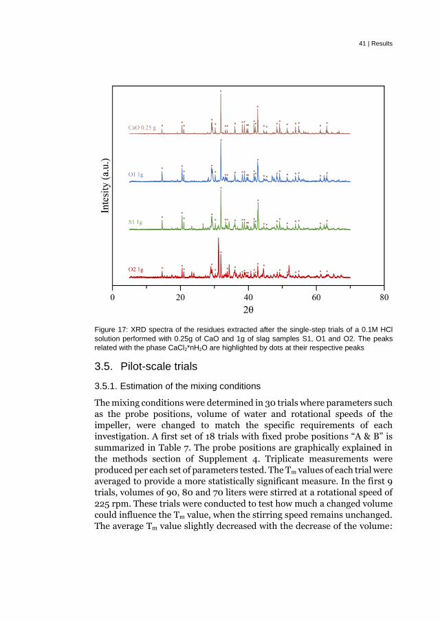
41 | Results

Figure 17: XRD spectra of the residues extracted after the single-step trials of a 0.1M HCl

solution performed with 0.25g of CaO and 1g of slag samples S1, O1 and O2. The peaks

related with the phase CaCl2*nH2O are highlighted by dots at their respective peaks

3.5. Pilot-scale trials

3.5.1. Estimation of the mixing conditions

The mixing conditions were determined in 30 trials where parameters such

as the probe positions, volume of water and rotational speeds of the

impeller, were changed to match the specific requirements of each

investigation. A first set of 18 trials with fixed probe positions “A & B” is

summarized in Table 7. The probe positions are graphically explained in

the methods section of Supplement 4. Triplicate measurements were

produced per each set of parameters tested. The Tm values of each trial were

averaged to provide a more statistically significant measure. In the first 9

trials, volumes of 90, 80 and 70 liters were stirred at a rotational speed of

225 rpm. These trials were conducted to test how much a changed volume

could influence the Tm value, when the stirring speed remains unchanged.

The average Tm value slightly decreased with the decrease of the volume:

Results | 42

from 10.3 s when a volume of 90 L was used to 9.7 s when a volume 80 L

was used, and finally it decreased to 9.3 s when a volume of 70 L was used.

The variation is in the range of 1 s. Nine other trials were conducted using

a volume 80 L stirred and 200 rpm, while volumes of 90 L and 70 L were

stirred at 175 rpm. Compared to the 225 rpm trials of the respective

volumes, when a volume of 80 L was stirred at 200 rpm there was a slight

increase in the Tm value. The average value was 10.3 s. The same average

Tm value of 10.3 s can also be found in the 70 L triplicate trials stirred at

175 rpm. The same average Tm value of 10.3 s was also found when a volume

of 90 L was stirred at 175 rpm.

Table 7: Mixing time trials with probe positions in A & B

Trial # Volume (L) Probe positions Speed (rpm) Tm (s) Average (s)

1 90 A & B 225 11

2 90 A & B 225 10

3 90 A & B 225 10 10.3

4 80 A & B 225 10

5 80 A & B 225 9

6 80 A & B 225 10 9.7

7 70 A & B 225 9

8 70 A & B 225 10

9 70 A & B 225 9 9.3

10 80 A & B 200 10

11 80 A & B 200 12

12 80 A & B 200 9 10.3

13 70 A & B 175 11

14 70 A & B 175 10

15 70 A & B 175 10 10.3

16 90 A & B 175 10

17 90 A & B 175 11

18 90 A & B 175 10 10.3

Twelve more additional trials were performed to test if different probe

positions could alter the Tm values. The results are compounded in Table

8. A water volume of 90 L was stirred at 225 rpm. The probes were

positioned at the bottom at a 90° angle compared to the configurations “A

& B”, namely the positions indicated as “C & D” in Supplement 4. Once

again, the average Tm value was comparable to previous results. The same

can be said when the trials are performed using the probe configuration “C

& D”, applied to volumes of 80 L and 70 L, stirred a 200 and 175 rpm,

43 | Results

respectively. Three more trials were performed with one probe located at

the bottom of the tank in position A and one located in radial symmetry to

it, but on the top of the tank, called position E. The Tm values when the

probes are positioned in positions “A & E” are 10s, 8s and 7s. Therefore,

when two probes are positioned at the bottom of the tank, either one of the

two takes more time to reach its final conductivity value compared to when

one is positioned at the bottom and one is positioned at the top of the tank.

Table 8: Mixing time trials with probe positions C & D and A & E

Trials #

Volume (L)

Probe positions

Speed (rpm) Tm (s)

Average (s)

19 90 C & D 225 10

20 90 C & D 225 9

21 90 C & D 225 9 9.3

22 80 C & D 200 9

23 80 C & D 200 9

24 80 C & D 200 10 9.3

25 70 C & D 175 9

26 70 C & D 175 10

27 70 C & D 175 10 9.6

28 90 A & E 225 10

29 80 A & E 225 8

30 70 A & E 225 7

3.5.2. Pilot-scale pH buffering trials

After the determination of the parameters able to maintain the mixing

conditions constant, regardless of a variation in volume, stepwise dosing

method trials were conducted using slag O1. The goal was to buffer the pH

values of 90 and 70 L of wastewaters. The results of the stepwise dosing

methodology are compounded in Table 9. Also, the trial with a 90 L volume

was replicated to check the replicability of the experiments. Even in this

case, slag O1 was able to reach the target pH value with additions of 33 g/L

and 29 g/L, for the 90 and 70 L volumes, respectively. These weights are

higher than the ones measured in precedent laboratory trials, which were

22.8 g and 14.7 to rise the pH of 1 L of acidic waste waters to the desired

pH target value.

Table 9: Up-scaled stepwise dosing trials characteristics (liters, rpm, total mass of added slag,

and final pH value).

Trial # Volume (L) Speed (rpm) weight (kg) pHfinal I-1 90 175 3 8.8

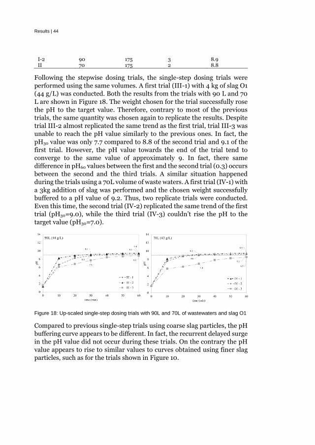
Results | 44

I-2 90 175 3 8.9 II 70 175 2 8.8

Following the stepwise dosing trials, the single-step dosing trials were

performed using the same volumes. A first trial (III-1) with 4 kg of slag O1

(44 g/L) was conducted. Both the results from the trials with 90 L and 70

L are shown in Figure 18. The weight chosen for the trial successfully rose

the pH to the target value. Therefore, contrary to most of the previous

trials, the same quantity was chosen again to replicate the results. Despite

trial III-2 almost replicated the same trend as the first trial, trial III-3 was

unable to reach the pH value similarly to the previous ones. In fact, the

pH30 value was only 7.7 compared to 8.8 of the second trial and 9.1 of the

first trial. However, the pH value towards the end of the trial tend to

converge to the same value of approximately 9. In fact, there same

difference in pH60 values between the first and the second trial (0.3) occurs

between the second and the third trials. A similar situation happened

during the trials using a 70L volume of waste waters. A first trial (IV-1) with

a 3kg addition of slag was performed and the chosen weight successfully

buffered to a pH value of 9.2. Thus, two replicate trials were conducted.

Even this time, the second trial (IV-2) replicated the same trend of the first

trial (pH30=9.0), while the third trial (IV-3) couldn’t rise the pH to the

target value (pH30=7.0).

Figure 18: Up-scaled single-step dosing trials with 90L and 70L of wastewaters and slag O1

Compared to previous single-step trials using coarse slag particles, the pH

buffering curve appears to be different. In fact, the recurrent delayed surge

in the pH value did not occur during these trials. On the contrary the pH

value appears to rise to similar values to curves obtained using finer slag

particles, such as for the trials shown in Figure 10.

45 | Results


3.6.1. Characterization of the sintered samples

EPMA spectroscopy was used to identify the different phases present in the

sintered samples. Figure 19 shows back-scatter electron (BSE) images of

the internal surfaces of the sintered pellets. The same phases are

recognizable across all the samples. The most abundant phase, identified

with the number 1, is the gray matrix which corresponds to FP. Phases

number 2 and 3 show typical signs of exsolution, naming the split in two

immiscible phases which occurs during cooling. Despite that point

determinations of those phases show different compositions, they can all

be expressed using the formula (Fe,Mg)Fe2O4. This has been confirmed by

the results from precedent studies68 also found the exsolution of

magnesioferrite (MgFe2O4, from hereafter MF) in FP. Phase 4 instead

appear to consisting of leftover pockets of FeO which do not recur in the

whole sample. MF visibly increases its presence the higher the FeO content

in the original powder mixture. In fact, it is barely visible in Figure 19a

(FeO 10wt%), while it clearly visible at the grain boundaries and at the

center of the grain in Figure 19b (FeO 15 wt%). Furthermore, it becomes

more prevalent in Figure 19c (FeO 20 wt%).

The qualitative observations made with EPMA spectroscopy are confirmed

with the results of the XRD analyses, as shown in Figure 20. The spectra

present the same peaks with different relative intensities. In particular, the

two phases identified by the analyses are FP and MF. The peaks related to

the latter increase in intensity with an increased initial FeO content, which

is in compliance with the results of EPMA determinations. In addition, FeO

was not detected in the XRD spectra, therefore its percentage can be

considered to be neglectable. Thus, all the sintered samples can be

considered binary system consisting of FP and MP, with an increasing

percentage of the latter, the more the initial FeO content in the sintered

powders.

Results | 46

Figure 19: BSE images of the cut surface of pellets of the samples 10 wt% FeO (a), 15 wt%

FeO (b) and 20 wt% FeO (c).

47 | Results

Figure 20: XRD spectra of the sintered samples. FP and MF peaks are used as reference to

evaluate the samples’ composition.

Mössbauer spectroscopy was used to quantify the amounts of FP and MF in

the samples, by identifying and quantifying the Fe species present in the

sample. In fact, it is expected that an ideal FP phase contains only Fe2+,

whereas Fe3+ belongs to a MF phase. Although, FP often contains Fe3+ as a

result of cation defects, which is a phenomenon that has been reported in

previous studies49,65 attributed to a high oxygen fugacity during sintering.

Nonetheless, different Fe3+ sites will exhibit different characteristics and

positions in the Mössbauer spectra, making it possible to distinguish

between each phase. The spectra were measured using the Doppler velocity

of the gamma-ray source in the range from -4 to +4 mm/s, so that a precise

assessment of the nonmagnetic FP phase can be achieved. The results

identified the presence of four different Fe sites, namely one Fe2+ and three

Fe3+ sites. All the sites are present in all the samples, even though they are

present in different ratios. The -4 to +4 mm/s spectra are shown on the left

side of Figure 21. By analyzing the characteristics and peak positions, it was

possible to assign two Fe3+ sites to the MF phase (short dots blue lines;

Results | 48

dash-dot light blue lines), while the remaining Fe3+ site (straight pink lines)

belongs to the FP phase, along with the sole Fe2+ one (dash-dot-dot green

lines). In this work, the Fe3+ component that belongs to the FP phase is

fitted with high-spin doublets, whereas in a similar study conducted by

Longo et al.84 it is fitted with low-spin singlets at the position marked with

the black arrows. The (FP Fe3+)/ΣFe ratios were calculated to be 1.2%, 2.1%,

2.6% for the 10, 15, 20 wt% FeO, respectively.

Figure 21: Mössbauer spectra of all the samples with velocity from -4 to 4 mm/s on the left,

with velocity from -12 to 12 mm/s on the right. Four sites are identified and each contribution

to the total spectra is unbundled. The sites are grouped into the phases of origin. The global

spectra are also presented (black marker and long-dotted red line). The black arrows point

the comparable peak position for the Fe3+site in the FP phase in a previous study84. Yellow

markers are used to identify the MF peaks (full marker: peaks that were visible in the -4, +4

mm/s range).

Once the slow velocity analyses were conducted to identify the species,

analyses with -12 to 12 mm/s velocities were performed to include all the

phase peaks. This allows for a more precise estimation of the ratios

49 | Results

between the Fe2+ and Fe3+ species. The difference between the two results

is shown by the yellow dots on the right side of Figure 21. Full dots are the

peaks belonging to to the -4 to 4 mm/s analysis, whereas the empty ones

are the peaks included by increasing the velocity. Since it can be

approximated that the MF phase does not contain Fe2+, and by considering

that the FP Fe3+ contribution is negligible (as lower now than calculated

before, given the increased range of analysis), the total Fe present in the FP

phase can be approximated by using the total Fe2+/ΣFe ratio. Thus, this

parameter allows to offset the heterogeneous composition (already shown

with XRD and EPMA analysis) across the sintered samples, when

analyzing their hydration behaviors. The ratios of Fe2+ to the total iron

concentration in the synthesized samples (Fe2+/ΣFe) were 72.3%, 66.6%

and 54.8% per the 10, 15, 20 wt% FeO samples, respectively. Overall,

Mössbauer spectroscopy clarifies what was qualitatively shown with other

characterization techniques. Specifically, the MF phase grows at the

expenses of the FP phase, as more FeO is used in the initial powder

mixture.

3.6.2. Hydration method design

TGA was selected to determine the weight loss associated with the

dehydration reactions of hydrated samples to estimate the amount of

adsorbed water. In addition, to determine whether TGA produces a

complete dehydration, the dehydration of a sample of an industrial grade

brucite was also performed. The weight loss obtained during the trials,

shown in Figure 22, was compared to calculations made by considering the

molar values associated with the dissociation reaction that transform

brucite into periclase. When molar quantities are considered, the

dehydration of brucite reduces its weight by 18 g*mol-1, which corresponds

to a 30.9% weight reduction. The weight loss obtained by TGA trial was

30.2%, which was close to the ideal calculation.

Results | 50

Figure 22: TG (straight-blue) and T°C (dotted-red) curve obtained during the dehydration of

standard grade sample of brucite

Following the validation of TGA, autoclave curing was performed on

industrial grade periclase samples to hydrate them into periclase. Different

ratios between MgO and H2O were tested to find the ideal parameters that

could provide a full hydration of the samples during autoclave curing.

Then, TGA was performed on th66e hydrated periclase samples to evaluate

the water adsorbed during the hydration process. The results of the TGA

trials and the relative parameters of the hydration in autoclave are shown

in Table 10. As is possible to notice, despite the different set of parameters

used, the weight loss associated with the dehydration of hydrated periclase

is roughly 30%. This result is compliant with both the dehydration of

industrial brucite and the ideal chemical calculation. Therefore, any of the

settings used in the trials could be used to hydrate the sintered samples.

Table 10: TGA trials performed on periclase samples after hydration with autoclave curing.

Trial #

MgO weight in autoclave (g)

H2O weight in autoclave (g)

TGA weight (mg)

Weight loss (mg)

Weight loss (%)

I 0.4050 2.5489 13.9000 -4.1848 -30.11 II 0.2192 2.5168 13.4900 -4.0863 -30.29

51 | Results

III 0.5059 6.5786 12.7600 -3.8388 -30.08

3.6.3. Hydration of ferropericlase

After the validation of the parameters of autoclave curing, the sintered

samples were hydrated. Per each sintered sample, three batches were

hydrated separately and TGA measurements were conducted on each

batch. Table 11 summarizes the parameters of the trials. As it is possible to

notice, the more the initial FeO wt%, the less is the weight loss, meaning

less water was adsorbed during the autoclave curing. Although, the

measurements present some scattering, and the differences in weight loss

between samples with different percentages of initial FeO, are sometimes

similar to the scattering of the same material.

Table 11: TGA results after the hydration of the sintered samples performed with autoclave

curing

Trial # FeO wt% TGA weight (mg) Weight loss (mg) Weight loss (%)

IV-1 10.20 12.3300 -3.4252 -27.78 IV-2 10.20 13.0600 -3.8594 -29.55 IV-3 10.20 14.0800 -4.1870 -29.74 V-1 15.01 13.5300 -3.7517 -27.73 V-2 15.01 13.8900 -3.7550 -27.03 V-3 15.01 12.6700 -3.3460 -26.41 VI-1 21.71 14.5500 -3.5460 -24.37 VI-2 21.71 13.0700 -3.2034 -24.51 VI-3 21.71 13.1300 -3.1574 -24.05

The sintered sample containing 15wt% of FeO was chosen for a final

characterization with XRD. The spectra after sintering, after autoclave and

after TGA were compared and collected in Figure 23. The phases present

are FP, MF and ferrobrucite. The XRD results also shows that FP is

completely transformed into ferrobrucite after the hydration with

autoclave curing, since all the FP peaks disappear. The results also show

that MF does not hydrate. In fact, all the MF peaks found in the spectrum

after sintering are also present after curing in autoclave. Finally, when the

material is dehydrated, the spectrum is reverted to its original values,

showing that the TGA determinations also completely dehydrates the

material.

Results | 52

Figure 23: XRD spectra of the sample with 15 wt% of FeO after sintering, autoclave curing,

and TGA.

53 | Discussion

4. Discussion

4.1. pH buffering trials of acidic waste waters or acidic

solutions with slag

Several slag samples have been sufficiently employed as a lime substitute

for the treatment of acidic waste waters. The boundary conditions around

which the slags are used highly affect their use and possible employment

in industrial applications. The weight of slag needed for the treatment of

the waste waters is highly influenced by parameters such as the slag

physical properties, method of addition (i.e. retention time), and the final

desired pH value.

The impact of physical properties on the buffering capability can be seen

first by comparing the effect of different PSDs on slag’s dissolution rates.

Between the single-step dosing method trials performed with slags with

PSD < 1mm and < 63 µm, the weight of slag used to the reach the same pH

values in 30 minutes was halved. This is because the dissolution is faster,

allowing the material to buffer the pH value to the same values in a shorter

time frame, when the average PSD value is lower. In fact, the final pH

values of the successful trials obtained when using the single-step dosing

method trials with PSD values < 63 µm are lower than the ones obtained

when using PSD values < 1mm, despite that they have identical pH30

values. Thus, since the final pH value is lower, it means that the dissolution

of slag happened at a faster rate, reaching the same value after 30 minutes.

This is also visible qualitatively, by observing the different pH curves. In

the PSD < 1mm single-step dosing trials, the pH values slowly rise after an

initial surge, followed by a second surge later in time. Instead, when

powders with PSD values < 63 µm are used, the successful trials are

characterized by a single surge that then plateaus and slowly approaches

the final pH value. The effect of a reduced particle size is also visible in the

results when using slags O2 and S2. When the PSD value of the slags was

< 1mm, the materials could not successfully complete the trials. Although,

when the slag’s PSD value was reduced, the materials were able to complete

the trials successfully (slag S2 only in the stepwise dosing trials). Therefore,

a reduction of the particle size is fundamental to reduce the amount of slag

used and to optimize the process, while allowing a more complete use of

the materials. In fact, the amount of the best performing slag compared to

lime in the single-step trials using a coarse PSD is roughly 8 to 10 times the

amount of lime needed to achieve similar pH values. From an industrial

perspective, this is hardly as a viable option. Although, when the PSD value

Discussion | 54

is decreased the weight of slag is reduced to 4 times the amount of lime.

This result indicates that it is possible to obtain an industrial

implementation of the technology if the PSD of the powders is low enough.

The quantity of slag needed for a successful trial is also dependent on the

method of addition, or the retention time. In fact, the amount of slag used

is different between the single-step and stepwise dosing method trials,

performed with the same slag. In general, the amount of slag needed is

lower for stepwise dosing method trials, compared to the single-step

dosing method trials. This is because the boundary condition to reach a pH

value of 9.0±0.2 by the 30th minute is absent. Also, the retention time of

slag is higher, especially for the weights inserted at the beginning of the

trial. In fact, when the first weight is inserted, its retention time is 30 min

per each slag addition that follows the first addition. This means that the

first weight addition has more time to react with the waste waters and to

increase the pH value. Also, different methods of addition benefit

differently from a reduced PSD value. In fact, the reduction of slag needed

in stepwise dosing method trials is lower than in the single-step dosing

trials. This is in line with the effect of an increased retention time that

allows even for slags with coarser PSD values to react more compared to

the single-step dosing trials. When the retention times are increased, the

ratio between lime and slag weights is also reduced. In fact, during the

stepwise dosing trials with PSD values < 63 µm, only three times the

amount of lime was needed to reach similar pH values. A similar ratio

between lime and slag was also found in the single-step trials when using

standard acidic solutions. When the boundary conditions of pH value and

time to reach it were removed, it was found that 1 g of the slag samples was

enough to reach a complete neutralization of the solutions. In contrast, it

was also calculated that 0.28 g of lime is needed to neutralize the same

solution. Moreover, the effect of a prolonged retention time is visible by

studies from Cunha et al.45,46, which evaluated the amount of sulfuric acid

needed to obtain a stable pH value of 1.5, when different oxidic products

are used. In this case, the dissolution of the minerals goes to completion,

until no more variation of the pH value is detected. In these studies, the

authors found that a sample of ladle slag has a neutralization potential (as

defined by the authors as the amount of sulfuric acid needed to obtain a

stable pH value of 1.5) 1.2 times higher than lime. In case of AOD slags it

was found a neutralization potential ranging from 0.75 to 0.8, BOF slags

from 0.6 to 0.84 and EAF slags from 0.71 to 0.92. Therefore, in these

experiments the slags samples were closer to lime in terms of efficiency

simply by changing the test conditions. In addition, the same effect is not

55 | Discussion

found when using lime, that due to its fast reaction rate and high solubility

yields the same necessary weight no matter on the method of addition.

Another aspect about the single-step dosing method trials is the

progression of the pH value over time. In the PSD < 1mm single-step

dosing trials the curves obtained have a peculiar trend. In fact, in almost

all the cases, the pH values have an initial surge followed by a plateau.

Successively, the pH values start to rise once again. This is more visible

with slag O1, despite the phenomenon appears with slag S1 too (Figure 2

Figure 8). This phenomenon becomes less evident when the PSD value is

reduced (Figure 10), but then it reoccurs also in successive experiments as

illustrated in Figure 11 and Figure 12. It is believed that the explanation for

this slope change in the curves is due to multiple factors. The most

important is that the pH scale is logarithmic, meaning that the difference

in H+ concentration (thereafter [H+]) decreases by 10 folds by each unit

increase. Moreover, the more alkali the solution in which the mineral is in

contact with, the lower is the dissolution rate of slag. This has been proved

both experimentally 81,82 and theoretically based on geochemical models,

used to determine the leaching of mineral phases present in steel slags 35.

In the same study, it is also demonstrated that in batch tests (like the one

conducted in this thesis) where the pH value is not kept constant, there’s a

solubility threshold value that makes it increasingly harder to increase the

pH value. In fact, De Windt et al 35 reported that at high pH values,

reducing the L/S ratio by a factor of 10, meaning using 10 times more the

weight of slag, only increases the pH value from 11.2 to 11.9. Similar results

were obtained by Mombelli et al.85, which found that only at high L/S ratios

the slag is significantly dissolved. However, when the L/S ratio is low, only

cortical reactions are detected. This is also in line with the results shown in

Supplement 3 and in paragraph 3.4.1, where a doubling of the weight of

slag translates to a progressively lower increase of the final pH values.

The two factors should be able to explain by themselves the pH value slopes

of the trials. Among all the trials, there are two recognizable patterns: the

two-plateaus system we mentioned before, compared to a single sharp rise

of the pH followed by a single plateau. The two trends appear to be weight

dependent: the latter occurs when the weight of slag is higher, while the

former occurs when it is lower. This is generally true for almost all the trials

conducted. This is because a low L/S ratio (more weight of slag) increases

the initial pH value to a level where the high alkalinity stifles a further

dissolution of the minerals. In contrast when the L/S ratio is higher, slag

dissolves more slowly and the apparent increase in dissolution rate is only

an artifact of the logarithmic nature of the pH value, coupled with the

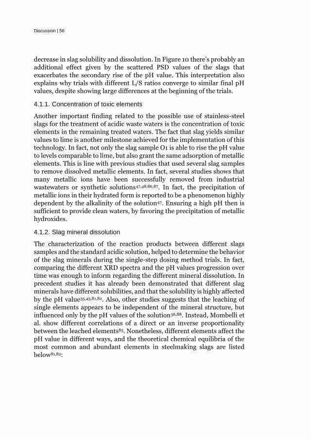
Discussion | 56

decrease in slag solubility and dissolution. In Figure 10 there’s probably an

additional effect given by the scattered PSD values of the slags that

exacerbates the secondary rise of the pH value. This interpretation also

explains why trials with different L/S ratios converge to similar final pH

values, despite showing large differences at the beginning of the trials.


Another important finding related to the possible use of stainless-steel

slags for the treatment of acidic waste waters is the concentration of toxic

elements in the remaining treated waters. The fact that slag yields similar

values to lime is another milestone achieved for the implementation of this

technology. In fact, not only the slag sample O1 is able to rise the pH value

to levels comparable to lime, but also grant the same adsorption of metallic

elements. This is line with previous studies that used several slag samples

to remove dissolved metallic elements. In fact, several studies shows that

many metallic ions have been successfully removed from industrial

wastewaters or synthetic solutions47,48,86,87. In fact, the precipitation of

metallic ions in their hydrated form is reported to be a phenomenon highly

dependent by the alkalinity of the solution47. Ensuring a high pH then is

sufficient to provide clean waters, by favoring the precipitation of metallic

hydroxides.

4.1.2. Slag mineral dissolution

The characterization of the reaction products between different slags

samples and the standard acidic solution, helped to determine the behavior

of the slag minerals during the single-step dosing method trials. In fact,

comparing the different XRD spectra and the pH values progression over

time was enough to inform regarding the different mineral dissolution. In

precedent studies it has already been demonstrated that different slag

minerals have different solubilities, and that the solubility is highly affected

by the pH value35,45,81,82. Also, other studies suggests that the leaching of

single elements appears to be independent of the mineral structure, but

influenced only by the pH values of the solution36,88. Instead, Mombelli et

al. show different correlations of a direct or an inverse proportionality

between the leached elements85. Nonetheless, different elements affect the

pH value in different ways, and the theoretical chemical equilibria of the

most common and abundant elements in steelmaking slags are listed

below81,82:

57 | Discussion

CaO(s)+ 2H+ → Ca2+ + H2O (2)

MgO(s)+ 2H+ → Mg2+ + H2O (3)

Al2O3(s)+ 6H+ → 2Al3+

+ 3H2O (4)

Al3+

+ 3H2O → Al(OH)3 (s) + 3H+ (5)

Al(OH)3(s)+ H2O → Al(OH)4-+ H+ (6)

SiO2(s)+2H2O → Si(OH)4(aq) (7)

Si(OH)4 (aq) → SiO(OH)3-+ H+ (8)

Ca and Mg have a similar chemistry, which leads to a removal of two H+

per ion dissolved. Si and Al have a more complicated chemistry, showing

different reactions that either remove or produce dissolved protons. Si for

instance is first hydrated in contact with water and then it dissociates in an

aqueous media, freeing a proton per each molecule of hydroxide. However,

aluminum oxide reacts with 6 protons, which translates in the dissolution

of two Al ions while forming 3 water molecules. The ions then recombine

with water to form Al hydroxide and a free proton. Successively, the

hydroxide further hydrates, releasing another proton.

Pourbaix diagrams of the aforementioned elements were calculated in a

precedent study using Factsage 6.189, and they are shown in Figure 24 to

determine in what pH ranges specific reactions are favored. In case of Si,

the generation of a proton is favored at high pH values, after reaching a pH

value of approximately 10. Therefore, during the single-step dosing

method trials, Si is not expected to contribute to the modification of the

solution’s pH value, since the pH is always lower than 10. On the other

hand, the removal of H+ due to the dissolution of Al is favored only at pH

values lower than 5. Afterwards, the favored chemical reaction is the free

extra protons by hydrating the Al ion. This means that Al counteracts the

alkalinity induced by Ca and Mg, generating H+ and lowering the pH value.

After reaching approximately a pH value of 9, Al hydroxide further

hydrates again, triggering a new reaction that generates a proton. Pourbaix

diagrams are expressing thermodynamically stable phases, whereas the

single-step trials are experiments far away from the equilibrium.

Nonetheless, it seems like the presence of Al in the slag is detrimental with

respect to the pH buffering capacity of the material.

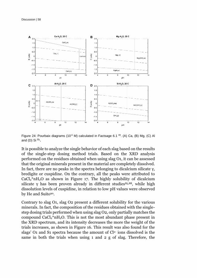
Discussion | 58

Figure 24: Pourbaix diagrams (10-6 M) calculated in Factsage 6.1 89. (A) Ca, (B) Mg, (C) Al

and (D) Si 81.

It is possible to analyze the single behavior of each slag based on the results

of the single-step dosing method trials. Based on the XRD analysis

performed on the residues obtained when using slag O1, it can be assessed

that the original minerals present in the material are completely dissolved.

In fact, there are no peaks in the spectra belonging to dicalcium silicate γ,

bredigite or cuspidine. On the contrary, all the peaks were attributed to

CaCl2*nH2O as shown in Figure 17. The highly solubility of dicalcium

silicate γ has been proven already in different studies85,88, while high

dissolution levels of cuspidine, in relation to low pH values were observed

by He and Suito90.

Contrary to slag O1, slag O2 present a different solubility for the various

minerals. In fact, the composition of the residues obtained with the single-

step dosing trials performed when using slag O2, only partially matches the

compound CaCl2*nH2O. This is not the most abundant phase present in

the XRD spectrum, and its intensity decreases the more the weight of the

trials increases, as shown in Figure 16. This result was also found for the

slags’ O1 and S1 spectra because the amount of Cl2- ions dissolved is the

same in both the trials when using 1 and 2 g of slag. Therefore, the

59 | Discussion

formation of CaCl2*nH2O is capped by the amount of chloric acid present

in the acidic solution. On the other hand, the relative percentage of other

phases increases, which diminishes the relative intensity of the peaks

corresponding to the compound CaCl2*nH2O. Although, this phenomenon

is particularly interesting to notice in slag O2, because it provides

information on the mineral phases. By comparing the results of the XRD

analysis of the residues from both trials, while also comparing them with

the original slag composition, almost all the major peaks can be assigned

to either merwinite, åkermanite or CaCl2*nH2O. In Figure 25 the spectra

of both trials are presented. The peaks belonging to each phase are

highlighted by different symbols. As seen in the trial performed with 1 g of

slag, åkermanite is the most abundant mineral phase, followed by the

compound CaCl2*nH2O and merwinite. In the trial using a 2 g addition of

slag, åkermanite remains the first mineral, while the other two swap

positions in terms of being the most prevalent phase. In fact, the

åkermanite content passes from being roughly 47% of the total sample in

the 1 g trial, to 54% in the 2 g trial. Furthermore, merwinite increases from

9% to 27%, while CaCl2*nH2O drops from 28% to 10% of the total sample.

This is evidence that, contrary to the minerals present in slag O1, the

minerals present in slag O2 are only partially dissolved. This is in line with

previous findings 81, where the solubility of merwinite, åkermanite and

dicalcium silicate γ were studied. At a pH value of 4, the three minerals do

not present meaningful differences in solubilities. Furthermore, at a pH

value of 7 the dissolution rate of åkermanite decreases, while it remains

almost the same for the other two phases. At a pH value 10 the solubility of

åkermanite and merwinite, drastically decreases, whereas the solubility of

dicalcium silicate γ is only modestly reduced. In other studies, åkermanite

is also shown to be less soluble compared to other minerals like bredigite

in a Tri-HCl solution of pH 7.491. This is reflected in the percentages of the

minerals found in the residues. Åkermanite is the mineral that decreases

its solubility the fastest. Therefore, after a certain threshold, the increase

in pH values is mostly determined by the dissolution of merwinite and

dicalcium silicate γ. Subsequently also the solubility of merwinite is

reduced while dicalcium silicate γ is completely dissolved.

Discussion | 60

Figure 25: XRD spectra of the residues extracted after the single-step trials of a 0.1M HCl solution performed with 1g and 2g of slag O2. The intensities are normalized to a 100 to aid a proper comparison between the spectra.

When looking at the XRD spectrum of the residues obtained after the

single-step dosing trials performed using 1 g of slag, similar results to the

ones performed when using slag O1 are found. Specifically, the most

abundant phase present is CaCl2*nH2O. This means that most of the

mineral phases in the starting composition of slag have dissolved during

the trial. Dicalcium silicate γ and bredigite show full dissociations when

using slag O1. However, åkermanite only partially dissolve in slag O2, due

to the low kinetic of its reactions with the acidic solution. In fact, faint

traces of åkermanite can be detected in the XRD spectrum of the residues

obtained with 1 g o f slag S1. This confirms that the mineral does not fully

dissolve during the trials. However, no traces of merwinite can be found in

the XRD spectrum. Therefore, it is assumed that most of it dissolve during

the trial. This is also in line with the behavior of slag O2, that shows that

very low levels of residual merwinite are present when the slag is not

overdosed (1 g trial).

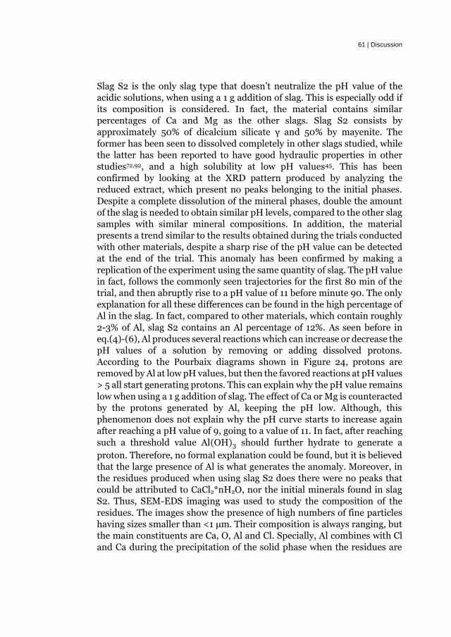
61 | Discussion

Slag S2 is the only slag type that doesn’t neutralize the pH value of the

acidic solutions, when using a 1 g addition of slag. This is especially odd if

its composition is considered. In fact, the material contains similar

percentages of Ca and Mg as the other slags. Slag S2 consists by

approximately 50% of dicalcium silicate γ and 50% by mayenite. The

former has been seen to dissolved completely in other slags studied, while

the latter has been reported to have good hydraulic properties in other

studies72,92, and a high solubility at low pH values45. This has been

confirmed by looking at the XRD pattern produced by analyzing the

reduced extract, which present no peaks belonging to the initial phases.

Despite a complete dissolution of the mineral phases, double the amount

of the slag is needed to obtain similar pH levels, compared to the other slag

samples with similar mineral compositions. In addition, the material

presents a trend similar to the results obtained during the trials conducted

with other materials, despite a sharp rise of the pH value can be detected

at the end of the trial. This anomaly has been confirmed by making a

replication of the experiment using the same quantity of slag. The pH value

in fact, follows the commonly seen trajectories for the first 80 min of the

trial, and then abruptly rise to a pH value of 11 before minute 90. The only

explanation for all these differences can be found in the high percentage of

Al in the slag. In fact, compared to other materials, which contain roughly

2-3% of Al, slag S2 contains an Al percentage of 12%. As seen before in

eq.(4)-(6), Al produces several reactions which can increase or decrease the

pH values of a solution by removing or adding dissolved protons.

According to the Pourbaix diagrams shown in Figure 24, protons are

removed by Al at low pH values, but then the favored reactions at pH values

> 5 all start generating protons. This can explain why the pH value remains

low when using a 1 g addition of slag. The effect of Ca or Mg is counteracted

by the protons generated by Al, keeping the pH low. Although, this

phenomenon does not explain why the pH curve starts to increase again

after reaching a pH value of 9, going to a value of 11. In fact, after reaching

such a threshold value Al(OH)3 should further hydrate to generate a

proton. Therefore, no formal explanation could be found, but it is believed

that the large presence of Al is what generates the anomaly. Moreover, in

the residues produced when using slag S2 does there were no peaks that

could be attributed to CaCl2*nH2O, nor the initial minerals found in slag

S2. Thus, SEM-EDS imaging was used to study the composition of the

residues. The images show the presence of high numbers of fine particles

having sizes smaller than <1 μm. Their composition is always ranging, but

the main constituents are Ca, O, Al and Cl. Specially, Al combines with Cl

and Ca during the precipitation of the solid phase when the residues are

Discussion | 62

extracted. That is why CaCl2*nH2O is not formed. Thus, it can be inferred

that the high solubility of mayenite (no traces of the original mineral are

found in the XRD spectra) mobilized high quantities of Al which

counteracted with the action of Ca and Mg in raising the pH of the acidic

solution.

In general, it is possible to connect the dissolution of the slag minerals with

the pH levels obtained during the single-step trials. In fact, slags O1 and

S1, which shows a complete dissolution of the mineral structure, also rise

the pH value to the highest levels. On the contrary slag O2 which only

partially dissolve its mineral structure, is less successful in rising the pH

per the same unit of mass. In addition, slag S2 dissolves completely, but it

does not perform as well as the other two slag samples.

4.1.3. Pilot-scale trials

Pilot-scale trials were conducted to determine if the technology could be

scalable to higher volumes. To do so, a physical water model was used to

simulate the mixing conditions of slag. This was done to ensure that the

mixing conditions remain the same when different volumes are tested. By

finding sets of parameters that can produce similar mixing conditions,

eventual variations in the L/S ratios in the single-step trials are due to the

chemical reactions alone and not due to kinetic factors. In this way, a

relationship between the amount of slag and waste waters can be drawn.

Another important reason for carrying on these tests was to ensure that a

homogenous mixing of slag was obtained before the first pH measurement

occurred. This, to guarantee that the sample’s value could be

representative of the whole volume. The mixing time trials showed similar

mixing conditions regardless of the choice of stirring speed, probe position

or volume of water being stirred. Therefore, the same stirring speed of 175

rpm was chosen for each volume during the pH buffering trials.

The stepwise and single-step dosing method trials show good replicability

of the experiments outside the laboratory conditions. The pH value

progression over time appears to be very similar to precedent trials

performed in laboratory settings, as seen by comparing Figure 18 with

Figure 10 and Figure 8. Although, the PSD value of the slag used was <350

µm, which constitutes 87% of the particles used in the trials with PSD

values < 1mm. Therefore, it was expected that the pH progression would

be similar to the one shown in Figure 8. However, the curves are more

similar to the trials showed in Figure 10, performed when using finer slag

particles. In fact, the trials are characterized by a sharp rise of the pH value

63 | Discussion

followed by a single plateau until the final pH value is reached. Despite the

attempts to produce comparable results, the different mixing conditions,

the use of a different batch of slag with a different PSD value and a varying

waste waters composition, surely influenced the results of the trials.

Another interesting factor to discuss is the variation of results when the

same mass of slag is used. In fact, both single-step trials using 90 and 70 L

volumes were performed three times using the same mass. Two trials per

each volume show almost overlapping values at each pH measurement, as

seen in Figure 18. This is in line with most of the replications performed

also in previous trials. Usually the same mass of slag, performs almost

identically every time the test is replicated. Although, this time, the third

trial of each set of experiments did not yield the same pH values. This could

be due to multiple factors, but the most probable explanation is the

variation in the waste waters compositions. In fact, both the first and

second trial of each set were conducted successively in the same morning,

whereas the third was performed in the afternoon. Due the large amount

of waste waters to treat, it was extracted from the industrial tanks each time

before the trials. Therefore, the composition was not kept constant. Also,

there is no guarantee that the same waters extracted had the same

composition all the time. Thus, it is possible to assume that a different

composition of the waste waters alters the solubility of the slag minerals,

which affects the progression of the pH values. Thus, it is important for

future trials in industrial trials that the waste waters composition is

checked before each single trial.

The quantity of slag needed to buffer the pH to the desired value seem to

follow a linear correlation with the amount of waste waters to treat, when

the mixing conditions are kept constant. In fact, the results of the single-

step dosing trials performed with 90 and 70 L of waste waters have been

plotted as a function of their L/S ratios. The results from the single-step

dosing trials can be seen in Figure 26. A linear regression between the two

trials has been plotted. Results from previous single-step dosing trials have

also been added as well to enable a comparison. As it is possible to notice,

the linear curve plotted well approximates the trend of the L/S ratio.

Moreover, the L/S ratio of the single-step dosing trials with PSD < 1mm

and < 63µm were included in the analysis. The L/S ratio of the single-step

dosing trials with PSD < 1mm fall very close to the regression line, as

expected since the powders have similar properties. In fact, from the

regression line it is expected that the trials using 1 L of waste waters should

have a weight of slag of almost 44 g. From the previous trials it is known

that the ideal quantity is 39 g. Therefore, considering the difference in

Discussion | 64

waste waters composition, PSD values of the two powders and mixing

conditions, the trials were successfully replicated to higher volumes with

comparable quantities with respect to the measured values during the

laboratory trials.

Figure 26: Linear regression of L/S ratio of the 90 L and 70 L single-step dosing trials. L/S ratios belonging to the precedent single-step dosing trials have been added for comparison.


The ferropericlase samples were successfully sintered using the precursor

material and method chosen, as seen in Figure 19 and Figure 20. Although,

non-negligible amounts of magnesioferrite were exsolved from the

ferropericlase matrix. This is a phenomenon well known in literature 66,

and it is due to the oxygen fugacity during sintering. The presence of

magnesioferrite is favored, the higher the presence of FeO in the

unsintered powders. Therefore, the oxygen fugacity needs to be controlled

in a way that accounts for an easier exsolution of the secondary phase,

rather than having fixed sintering conditions such as the one used in the

current study. Alternatively, the oxygen fugacity can be reduced to the

point where even an increase of the FeO value doesn’t allow for the

exsolution of magnesioferrite. Nonetheless, despite the presence of

65 | Discussion

magnesioferrite, the samples were considered to be homogeneous enough

to conduct the study.

The hydration and dehydration techniques used on the sintered samples

were validated by carrying out several trials. First, a TGA test on a sample

of industrial brucite was performed and the weight loss shown in Figure 22

was compared to ideal calculations made using molar values. The value

measured with TGA was 30.2%, which was very close to the ideal case of

30.9%. Therefore, it was proven that the parameters selected could provide

the complete dehydration of the material. Successfully, the parameters in

autoclave curing were selected and several samples of periclase were

hydrated into brucite. In addition, TGA measurements were conducted to

determine their weight losses. In this way, it was possible to find the

parameters that could provide a full hydration of the materials, by

confronting the weight loss obtained during the TGA determinations

performed on the hydrated periclase and industrial brucite. Once the

parameters were determined with the use of periclase and brucite,

autoclave curing and TGA trials were conducted on the sintered samples.

The weight loss measured during the TGA determinations of the sintered

samples (Table 11), can be plotted as a function of the Fe content in the

samples. Despite that it is known that the sintered samples present non-

neglectable amounts of magnesioferrite, only the Fe present in the

ferropericlase should be considered. As seen in Figure 20, this is because

magnesioferrite does not hydrate during autoclave curing. It is possible to

consider only the Fe2+ content, measured with Mössbauer spectroscopies,

to approximate the amount of ferropericlase present, and obtain a better

estimation of water absorption. This is done by purposely neglecting the

quantity of Fe3+ in the ferropericlase, which although was estimated to be

less than 1% for each sample. In addition, it is not known how much the

presence of Fe3+ in the mineral matrix affects its water absorption. Figure

27 shows the relationship between the weight loss during TGA

measurements as a function of the Fe2+ content. A linear regression has

also been added to the figure. Furthermore the data from a study by Hou

et. al77, which performed a similar analysis to the one conducted in this

section of the thesis, has also been added to the figure. The sample was

chosen as it was the one with composition most similar to the ones from

the current study. In addition, the results from the TGA trials were

compared to an ideal system consisting of unsintered powders of brucite

and FeO. In this ideal case, the powders were dehydrated and thereafter

their weight losses were calculated based on molar values. The weight loss

is caused by the dehydration of brucite only, as FeO acts as a bulk weight.

Discussion | 66

The comparison to this ideal system shows that the weight loss associated

with the increasing presence of Fe in the FP matrix, is higher than what can

be explained by a simple substitution of one molecule of MgO with one

molecule of FeO. If that would have been the case, then the dehydration

should have followed the unsintered powders line. Instead, the reduction

in dehydration, corresponding to the absorption of water, decreases with

an increased Fe content in the FP. Moreover, the point extracted from the

study made by Hou et at.77 shows a good fitting with the regression line.

Thus, the results of this study show that the water adsorption of

ferropericlase decreases linearly with an increase of the Fe content,

although the samples present very low and very similar percentages of Fe

to consolidate this hypothesis. Finally, the reduction in water adsorption

compared to pure MgO is 6%, when the initial FeO content is 20wt%.

Although, it is unknown how much the water adsorption influences the

swelling of the final product. The swelling is influenced mostly by

parameters such as powders compaction, which is in turn is influenced by

powder homogeneity, particle size and the load applied to the powders

during the volumetric expansion tests11. Moreover, the material is not

usually used in isolation but as a blend with other aggregates and binders.

Therefore, the individual effect on swelling are hard to predict and some of

the studies on this topic preferred to focus on the different water

adsorption as a proxy of swelling93.

67 | Discussion

Figure 27: Reduction of sample weight (ΔW%) after TGA analyses on the hydrated samples plotted as a function of the calculated Fe2+ at%. The dash-dotted line represents the hydration behavior of an unsintered powder mixture consisting of MgO and FeO, where MgO is fully transformed in brucite and FeO acts as bulk material. The dotted line represents the linear regression of all TGA measurements. For comparison, a data point of composition 80mol%MgO−20mol%FeO from the study made by Hou at al. 77 has been added.

Hou et al.

Discussion | 68

69 | Conclusions

5. Conclusions

The aim of this thesis was to evaluate possible strategies that could enhance

the recycling of metallurgical slags. In particular, the thesis focused on two

kinds of steel by-products: BOF slags and stainless-steel slags. The

recycling of the latter is the most problematic one, as it currently cannot be

used in the state-of-the-art applications such as in the construction

industry as a binder to produce cement or asphalt. Therefore, most of the

studies related to this thesis focused on designing a new application for its

recycling. From Supplement 1 to Supplement 3, many studies have been

conducted to test the use of stainless-steel slags as a substitute of lime for

the pH buffering of acidic waste waters. In Supplement 1, experiments have

been developed to test this new application, by using 4 different stainless-

steel slags. In addition, pH buffering trials, along with experiments aimed

at testing the concentrations of metallic elements in the treated waters

have been conducted. The results have been compared to the same

experiments performed using a standard grade lime product. In

Supplement 2, the use of slag has been optimized to reduce the amount of

material needed. Furthermore, in Supplement 4 the scalability of the

application is tested, by up scaling the volume of waste waters treated. In

Supplement 3, the dissolution of the minerals present in the slag samples

is evaluated. Supplement 5 focuses on the recycling of BOF slags which is

impeded by the swelling of MgO and CaO when subjected to water or

humidity, which causes the premature degradation of the final product

where the slag is employed. Therefore, the hydration of ferropericlase is

studied, to determine the expansion of this mineral phase.

The main findings of each supplement are summarized in Table 12. The

table used the same framework used in Table 1, to compare the initial

proposed solutions with the obtained results from each supplement. A

more thorough description of the main findings of each supplement follows

the table for a more in-depth look at the results of the several studies.

Table 12: Main findings of each study related to the initial experimental setup and proposed solution.

Proposed Solution Experimental Setup Main Results

Development of an alternative application as lime substitute for acidic

Supplement 1: Preliminary study aimed at testing different slags as pH buffering agents

Two slags, out of four tested, are successfully employed as lime substitutes to rise the pH of industrial acidic waste waters to the desired value. The concentration of

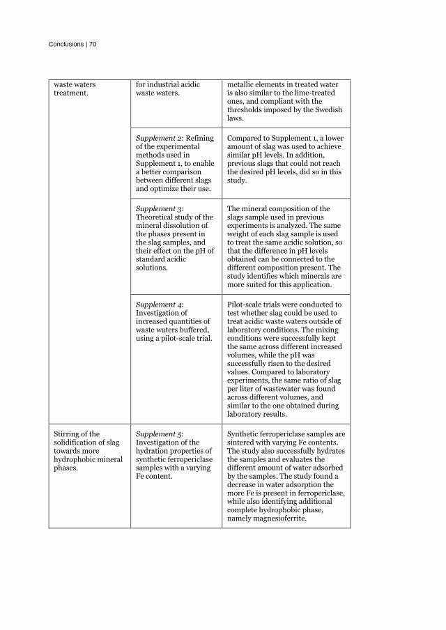
Conclusions | 70

waste waters treatment.

for industrial acidic waste waters.

metallic elements in treated water is also similar to the lime-treated ones, and compliant with the thresholds imposed by the Swedish laws.

Supplement 2: Refining of the experimental methods used in Supplement 1, to enable a better comparison between different slags and optimize their use.

Compared to Supplement 1, a lower amount of slag was used to achieve similar pH levels. In addition, previous slags that could not reach the desired pH levels, did so in this study.

Supplement 3: Theoretical study of the mineral dissolution of the phases present in the slag samples, and their effect on the pH of standard acidic solutions.

The mineral composition of the slags sample used in previous experiments is analyzed. The same weight of each slag sample is used to treat the same acidic solution, so that the difference in pH levels obtained can be connected to the different composition present. The study identifies which minerals are more suited for this application.

Supplement 4: Investigation of increased quantities of waste waters buffered, using a pilot-scale trial.

Pilot-scale trials were conducted to test whether slag could be used to treat acidic waste waters outside of laboratory conditions. The mixing conditions were successfully kept the same across different increased volumes, while the pH was successfully risen to the desired values. Compared to laboratory experiments, the same ratio of slag per liter of wastewater was found across different volumes, and similar to the one obtained during laboratory results.

Stirring of the solidification of slag towards more hydrophobic mineral phases.

Supplement 5: Investigation of the hydration properties of synthetic ferropericlase samples with a varying Fe content.

Synthetic ferropericlase samples are sintered with varying Fe contents. The study also successfully hydrates the samples and evaluates the different amount of water adsorbed by the samples. The study found a decrease in water adsorption the more Fe is present in ferropericlase, while also identifying additional complete hydrophobic phase, namely magnesioferrite.

71 | Conclusions

The following can be concluded by the results of the supplements:

o Several stainless-steel slags have been successfully employed for the

pH buffering of acidic waste waters, as illustrated in Supplements 1 and

2. Depending on the method of addition, properties of the material

used and boundary conditions, different quantities of slag were found

to be needed to rise the pH value to the desired values. When the PSD

of the sample was kept < 1mm (in Supplement 1), the weight of slag to

buffer the pH value of 1 L of acidic waste waters has been found to be

between 39 g/L to 49 g/L, depending on the sample. That correspond

approximately to between 10 to 12 times the mass of lime needed to

buffer the pH value, when using the same quantity of acidic waste

waters. However, in Supplement 2 the PSD values of the slag samples

were reduced to < 63 µm. As a result, the quantities became 20 and 23

g/L, respectively. That translates in 4 to 5 times the weight of lime.

Moreover, samples with coarser PSD values in Supplement 1 were

unable to buffer the pH to the desired values. Although, after the

reduction in PSD all the samples could successfully complete the trials.

In addition, when the PSD value is further reduced to 25-50 µm and

both time and pH values restrictions were removed, as shown in

Supplement 3, successful neutralizations were conducted with

quantities close to 3 times the amount of lime. Depending on the

process specifications and needs, different quantities of slag are

needed. Slag appears to have a slower dissolution rate than lime, so it

requires higher retention times in the acidic baths. In addition, slag

samples cannot reach the same pH values obtained by lime, although

lime is harder to control when pH values close to neutral are needed.

Therefore, when neutral pH values are required, slag can act as a better

reactant compared to lime.

o In Supplement 1 it was found that the water treated with slag does not

possess higher percentages of metallic elements such as Cr, Ni, Mo,

compared to the one treated with lime. This is an important discovery,

considering that the stainless-steel slag is prone to leaching. Also,

that’s why it is not safely employed in current the state-of-the-art

recycling applications. The results show that with the method of

additions and retention times used, the slag is equivalent to lime in

adsorbing metallic elements from the waste waters. Along with the pH

buffering results, the low level of metallic element dissolved in the

waste waters is an important prerequisite for the use of slags in such

applications.

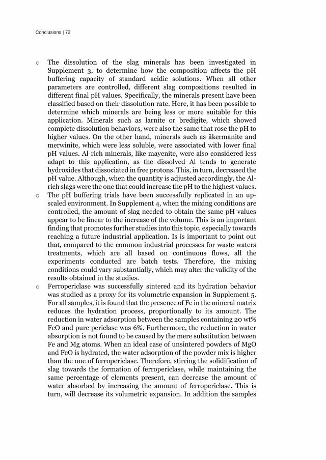
Conclusions | 72

o The dissolution of the slag minerals has been investigated in

Supplement 3, to determine how the composition affects the pH

buffering capacity of standard acidic solutions. When all other

parameters are controlled, different slag compositions resulted in

different final pH values. Specifically, the minerals present have been

classified based on their dissolution rate. Here, it has been possible to

determine which minerals are being less or more suitable for this

application. Minerals such as larnite or bredigite, which showed

complete dissolution behaviors, were also the same that rose the pH to

higher values. On the other hand, minerals such as åkermanite and

merwinite, which were less soluble, were associated with lower final

pH values. Al-rich minerals, like mayenite, were also considered less

adapt to this application, as the dissolved Al tends to generate

hydroxides that dissociated in free protons. This, in turn, decreased the

pH value. Although, when the quantity is adjusted accordingly, the Al-

rich slags were the one that could increase the pH to the highest values.

o The pH buffering trials have been successfully replicated in an up-

scaled environment. In Supplement 4, when the mixing conditions are

controlled, the amount of slag needed to obtain the same pH values

appear to be linear to the increase of the volume. This is an important

finding that promotes further studies into this topic, especially towards

reaching a future industrial application. Is is important to point out

that, compared to the common industrial processes for waste waters

treatments, which are all based on continuous flows, all the

experiments conducted are batch tests. Therefore, the mixing

conditions could vary substantially, which may alter the validity of the

results obtained in the studies.

o Ferropericlase was successfully sintered and its hydration behavior

was studied as a proxy for its volumetric expansion in Supplement 5.

For all samples, it is found that the presence of Fe in the mineral matrix

reduces the hydration process, proportionally to its amount. The

reduction in water adsorption between the samples containing 20 wt%

FeO and pure periclase was 6%. Furthermore, the reduction in water

absorption is not found to be caused by the mere substitution between

Fe and Mg atoms. When an ideal case of unsintered powders of MgO

and FeO is hydrated, the water adsorption of the powder mix is higher

than the one of ferropericlase. Therefore, stirring the solidification of

slag towards the formation of ferropericlase, while maintaining the

same percentage of elements present, can decrease the amount of

water absorbed by increasing the amount of ferropericlase. This is

turn, will decrease its volumetric expansion. In addition the samples

73 | Conclusions

also contained traces of a phase having a composition of (Mg,Fe)Fe2O4,

which was also found to be hydrophobic.

Based on to the results of the supplements, it is possible to show how

different steps can be taken to increase the recycling of metallurgical slags,

in particular BOF slags and different types of stainless-steel slags.

Regarding the former, the thesis proposes a solution to control the

solidification phase of the material, stirring towards the formation of

ferropericlase, and to avoid the formation of f-MgO. Avoiding the

formation of periclase, reduces if not stifles entirely, the water adsorption

of water and thus its volumetric expansion. This increases the possibilities

that the material can be employed more successfully in the applications

where a volumetric stability is required, which coincide with the common

state-of-the-art ones. On the other hand, when slag cannot be employed in

such applications, such as stainless-steel slags, the thesis suggests a new

application that can be explored further, as a substitute to lime in the pH

buffering of acidic waste waters as well for water treatments.

When slag is successfully employed in recycling applications, substituting

the use of raw materials, two main environmental benefits are achieved.

First, the steel producers reduce their landfilled output. This can either

generate more revenues by creating new products, or simply by reducing

the costs associated with landfilling. In addition, the construction industry

is one of the harder sectors to decarbonize. Specifically, a big part of the

emissions is caused by the extraction phase. Therefore, by reusing

secondary mineral sources, less raw materials are employed. This, in turn,

corresponds to a net reduction of CO2 which is generated holistically.

Therefore, it is of the uppermost importance to increase, as much as

possible, the employment of slags in recycling application, reducing its

landfilling.

Conclusions | 74

75 | Future Work

6. Future Work

In this thesis the use of stainless-steel slag as a lime substitute for the

neutralization has been thoroughly studied. The results are encouraging,

as the material matched the performances of lime both with respect to high

levels of pH values reached and low concentrations of metallic ions in the

treated waters. Moreover, the technology has been validated in different

environments than the small beakers where it was tested at first. Industrial

up-scale trial showed that the same results can be achieved even when the

volumes are increased by approximately 100 folds. In addition, the

dissolution of several minerals in steel slag has been investigated, selecting

the most performing one. Overall, slag showed a slower dissolution of lime,

which can be detrimental to applications where the retention time is

limited. The studies conducted only used batch tests conditions, whereas

some industrial processes present situations of constant flow. Therefore,

given the high dependence of the slag dissolution by the kinetic conditions,

the use of slag for such application should be investigated further in more

similar environments. In addition, grinding the powders to appropriate

particle sizes might be necessary to guarantee a good performance of the

materials, especially when the retention times are limited. Therefore, an

evaluation should be conducted to evaluate what operations are

economically feasible in an industrial setting. Finally, the use of slag

instead of lime for the treatment of waste waters necessarily produce new

by-products and changes to the processes where they are employed that

haven’t been investigated in this thesis.

The hydration of ferropericlase showed that the presence of FeO alters

substantially the water absorbed by the material. However, the test

conducted were made on a narrow range of FeO content, meaning that the

relationship between hydration of ferropericlase and Fe content was hard

to evaluate. Moreover, the sintering method produced some external

hydrophobic phases that increased the uncertainties related to the results

of the tests. Nonetheless, the hydration and dehydration tests showed

promising and reliable results. Therefore, the relationship between

hydration and Fe content should be further investigated by increasing the

ranges of FeO contents in the ferropericlase samples. Moreover, the

sintering conditions should be further improved so no exsolution of

magnesioferrite happens. To increase even further the reliability of TGA

tests, more trials on the same samples are recommended. In addition, the

relationship between water absorption and volumetric expansion should

Future Work | 76

be tested once the relationship between the Fe content and water

absorption has been found.

77 | References

References

1. Yildirim, I. Z. & Prezzi, M. Chemical, Mineralogical, and Morphological Properties of Steel

Slag. Adv. Civ. Eng. 2011, 1–13 (2011).

2. Huaiwei, Z. & Xin, H. An overview for the utilization of wastes from stainless steel

industries. Resour. Conserv. Recycl. 55, 745–754 (2011).

3. European Steel in Figures 2020. https://www.eurofer.eu/publications/brochures-

booklets-and-factsheets/european-steel-in-figures-2020/.

4. Holappa, L., Kekkonen, M., Jokilaakso, A. & Koskinen, J. A Review of Circular Economy

Prospects for Stainless Steelmaking Slags. J. Sustain. Metall. (2021) doi:10.1007/s40831-

021-00392-w.

5. Piatak, N. M., Parsons, M. B. & Seal, R. R. Characteristics and environmental aspects of

slag: A review. Appl. Geochem. 57, 236–266 (2015).

6. Lewis, D. W. Properties and uses of iron and steel slags. in 11 (National Slag Association,

1982).

7. Fisher, L. V. & Barron, A. R. The recycling and reuse of steelmaking slags — A review.

Resour. Conserv. Recycl. 146, 244–255 (2019).

8. Verhasselt, A. & Choquet, F. Steel slags as unbound aggregate in road construction:

problems and recommendations. in Unbound Aggregates in Roads 204–211 (Elsevier,

1989). doi:10.1016/B978-0-408-04355-7.50031-5.

9. Mikhail, S. A. & Turcotte, A. M. Thermal behaviour of basic oxygen furnace waste slag.

Thermochim. Acta 263, 87–94 (1995).

10. Motz, H. & Geiseler, J. Products of steel slags an opportunity to save natural resources.

Waste Manag. 9 (2001).

11. Wang, G., Wang, Y. & Gao, Z. Use of steel slag as a granular material: Volume expansion

prediction and usability criteria. J. Hazard. Mater. 184, 555–560 (2010).

12. Xie, J. Recycling of basic oxygen furnace slag in asphalt mixture: Material

characterization & moisture damage investigation. Constr. Build. Mater. 8 (2012).

References | 78

13. Ortega-López, V., Manso, J. M., Cuesta, I. I. & González, J. J. The long-term accelerated

expansion of various ladle-furnace basic slags and their soil-stabilization applications.

Constr. Build. Mater. 68, 455–464 (2014).

14. Chen, Z. et al. Utilization of gneiss coarse aggregate and steel slag fine aggregate in asphalt

mixture. Constr. Build. Mater. 93, 911–918 (2015).

15. Kambole, C., Paige-Green, P., Kupolati, W. K., Ndambuki, J. M. & Adeboje, A. O. Basic

oxygen furnace slag for road pavements: A review of material characteristics and

performance for effective utilisation in southern Africa. Constr. Build. Mater. 148, 618–

631 (2017).

16. Liu, C., Guo, M., Pandelaers, L., Blanpain, B. & Huang, S. Stabilization of Free Lime in

BOF Slag by Melting and Solidification in Air. Metall. Mater. Trans. B 47, 3237–3240

(2016).

17. Shen, H. & Forssberg, E. An overview of recovery of metals from slags. Waste Manag. 23,

933–949 (2003).

18. Tossavainen, M. et al. Characteristics of steel slag under different cooling conditions.

Waste Manag. 27, 1335–1344 (2007).

19. Reddy, A. S., Pradhan, R. K. & Chandra, S. Utilization of Basic Oxygen Furnace (BOF) slag

in the production of a hydraulic cement binder. Int. J. Miner. Process. 79, 98–105 (2006).

20. Crutzen, P. J. Geology of mankind TheAnthropocene. 1.

21. Kirchherr, J., Reike, D. & Hekkert, M. Conceptualizing the circular economy: An analysis

of 114 definitions. Resour. Conserv. Recycl. 127, 221–232 (2017).

22. Rashid, A., Asif, F. M. A., Krajnik, P. & Nicolescu, C. M. Resource Conservative

Manufacturing: an essential change in business and technology paradigm for sustainable

manufacturing. J. Clean. Prod. 57, 166–177 (2013).

23. Lieder, M. & Rashid, A. Towards circular economy implementation: a comprehensive

review in context of manufacturing industry. J. Clean. Prod. 115, 36–51 (2016).

79 | References

24. Ghisellini, P., Cialani, C. & Ulgiati, S. A review on circular economy: the expected

transition to a balanced interplay of environmental and economic systems. J. Clean. Prod.

114, 11–32 (2016).

25. Bocken, N. M. P., Short, S. W., Rana, P. & Evans, S. A literature and practice review to

develop sustainable business model archetypes. J. Clean. Prod. 65, 42–56 (2014).

26. Chertow, M. R. Industrial Symbiosis: Literature and Taxonomy. Annu. Rev. Energy

Environ. 25, 313–337 (2000).

27. Maslehuddin, M., Sharif, A. M., Shameem, M., Ibrahim, M. & Barry, M. S. Comparison of

properties of steel slag and crushed limestone aggregate concretes. Constr. Build. Mater.

17, 105–112 (2003).

28. Jernkontoret. Stålindustrin gör mer än stål. Handbok för restprodukter 2018. 56 (2018).

29. Bayless, E. R. & Schulz, M. S. Mineral precipitation and dissolution at two slag-disposal

sites in northwestern Indiana, USA. Environ. Geol. 45, 252–261 (2003).

30. Bayless, E. R. et al. District Chief U.S. Geological Survey.

31. Bayless, E. R., Bullen, T. D. & Fitzpatrick, J. A. Use of 87Sr/86Sr and δ11B to Identify Slag-

Affected Sediment in Southern Lake Michigan. Environ. Sci. Technol. 38, 1330–1337

(2004).

32. Roadcap, G. S., Kelly, W. R. & Bethke, C. M. Geochemistry of Extremely Alkaline (pH >

12) Ground Water in Slag-Fill Aquifers. Groundwater 43, 806–816 (2005).

33. Navarro, A., Cardellach, E., Mendoza, J. L., Corbella, M. & Domènech, L. M. Metal

mobilization from base-metal smelting slag dumps in Sierra Almagrera (Almería, Spain).

Appl. Geochem. 23, 895–913 (2008).

34. Standard - Characterization of waste - Leaching - Compliance test for leaching of granular

waste materials and sludges - Part 2: One stage batch test at a liquid to solid ratio of 10

l/kg for materials with particle size below 4 mm (without or with size reduction)SS-EN

12457-2. Svenska institutet för standarder, SIS

https://www.sis.se/en/produkter/environment-health-protection-safety/wastes/solid-

wastes/ssen124572/.

References | 80

35. De Windt, L., Chaurand, P. & Rose, J. Kinetics of steel slag leaching: Batch tests and

modeling. Waste Manag. 31, 225–235 (2011).

36. Loncnar, M. et al. Study of the leaching behaviour of ladle slags by means of leaching tests

combined with geochemical modelling and mineralogical investigations. J. Hazard.

Mater. 317, 147–157 (2016).

37. Engström, F. et al. Leaching Behavior of Aged Steel Slags. Steel Res. Int. 85, 607–615

(2014).

38. Seignez, N., Gauthier, A., Bulteel, D., Damidot, D. & Potdevin, J.-L. Leaching of lead

metallurgical slags and pollutant mobility far from equilibrium conditions. Appl.

Geochem. 23, 3699–3711 (2008).

39. Bäverman, C., Sapiej, A., Moreno, L. & Neretnieks, I. Serial batch tests performed on

municipal solid waste incineration bottom ash and electric arc furnace slag, in

combination with computer modelling. Waste Manag. Res. 15, 55–71 (1997).

40. Piatak, N. M., Seal, R. R. & Hammarstrom, J. M. Mineralogical and geochemical controls

on the release of trace elements from slag produced by base- and precious-metal smelting

at abandoned mine sites. Appl. Geochem. 19, 1039–1064 (2004).

41. Parsons, M. B., Bird, D. K., Einaudi, M. T. & Alpers, C. N. Geochemical and mineralogical

controls on trace element release from the Penn Mine base-metal slag dump, California.

Appl. Geochem. 16, 1567–1593 (2001).

42. Gbor, P. K., Ahmed, I. B. & Jia, C. Q. Behaviour of Co and Ni during aqueous sulphur

dioxide leaching of nickel smelter slag. Hydrometallurgy 57, 13–22 (2000).

43. Kim, E. et al. Selective recovery of Cr from stainless steel slag by alkaline roasting followed

by water leaching. 10 (2015).

44. Pikna, L. et al. Recovery of Chromium from Slags Leachates by Electrocoagulation and

Solid Product Characterization. Metals 10, 1593 (2020).

45. Cunha, M. L., Gahan, C. S., Menad, N. & Sandström, Å. Leaching Behaviour of Industrial

Oxidic By-Products: Possibilities to Use as Neutralisation Agent in Bioleaching. Adv.

Mater. Forum IV 5.

81 | References

46. Cunha, M. L., Gahan, C. S., Menad, N. & Sandström, Å. Possibilities to use oxidic by-

products for precipitation of Fe/As from leaching solutions for subsequent base metal

recovery. Miner. Eng. 21, 38–47 (2008).

47. Forsido, T., McCrindle, R., Maree, J. & Mpenyana-Monyatsi, L. Neutralisation of acid

effluent from steel manufacturing industry and removal of metals using an integrated

electric arc furnace dust slag/lime process. SN Appl. Sci. 6 (2019).

48. Zvimba, J. N., Siyakatshana, N. & Mathye, M. Passive neutralization of acid mine drainage

using basic oxygen furnace slag as neutralization material: experimental and modelling.

Water Sci. Technol. 75, 1014–1024 (2017).

49. Qian, G. R., Sun, D. D., Tay, J. H. & Lai, Z. Y. Hydrothermal reaction and autoclave

stability of Mg bearing RO phase in steel slag. Br. Ceram. Trans. 101, 159–164 (2002).

50. Brännberg Fogelström, J., Lundius, A. & Pousette, H. Neutralizing acidic wastewater

from the pickling process using slag from the steelmaking process : A pilot study in

project "Neutralsyra" (2017).

51. Figueira, R. M. & Szekely, J. Turbulent Fluid Flow Phenomena in a Water Model of an

AOD System. Metall. Trans. B 16, 67–75 (1985).

52. Bjurström, M., Tilliander, A., Iguchi, M. & Jönsson, P. Physical-modeling Study of Fluid

Flow and Gas Penetration in a Side-blown AOD Converter. ISIJ Int. 46, 523–529 (2006).

53. Cabaret, F., Bonnot, S., Fradette, L. & Tanguy, P. A. Mixing Time Analysis Using

Colorimetric Methods and Image Processing. Ind Eng Chem Res 46, 5032–5042 (2007).

54. Wuppermann, C. et al. A Novel Approach to Determine the Mixing Time in a Water Model

of an AOD Converter. ISIJ Int. 52, 1817–1823 (2012).

55. Samuelsson, P., Ternstedt, P., Tilliander, A., Appell, A. & Jönsson, P. G. Use of physical

modelling to study how to increase the production capacity by implementing a novel

oblong AOD converter. Ironmak. Steelmak. 45, 335–341 (2018).

56. Wei, J.-H., Zhu, H.-L., Chi, H.-B. & Wang, H.-J. Physical Modeling Study on Combined

Side and Top Blowing AOD Refining Process of Stainless Steel: Gas Stirring and Fluid

Flow Characteristics in Bath. ISIJ Int. 50, 17–25 (2010).

References | 82

57. Wei, J.-H., Zhu, H.-L., Chi, H.-B. & Wang, H.-J. Physical Modeling Study on Combined

Side and Top Blowing AOD Refining Process of Stainless Steel: Fluid Mixing

Characteristics in Bath. ISIJ Int. 50, 26–34 (2010).

58. Wei J.-H. et al. Water modelling study of fluid flow and mixing characteristics in bath

during AOD process. Ironmak. Steelmak. 26, 363–371 (1999).

59. Zhou, X., Ersson, M., Zhong, L., Yu, J. & Jönsson, P. Mathematical and Physical

Simulation of a Top Blown Converter. Steel Res. Int. 85, 273–281 (2014).

60. Ternstedt, P., Tilliander, A., Jönsson, P. G. & Iguchi, M. Mixing Time in a Side-Blown

Converter. ISIJ Int. 50, 663–667 (2010).

61. Narygina, O. et al. High-pressure experimental and computational XANES studies of ( Mg

, Fe ) ( Si , Al ) O 3 perovskite and (Mg,Fe)O ferropericlase as in the Earth’s lower mantle.

Phys. Rev. B 79, (2009).

62. Kung, J., Li, B., Weidner, D. J., Zhang, J. & Liebermann, R. C. Elasticity of (Mg 0.83 ,Fe

0.17 )O ferropericlase at high pressure: ultrasonic measurements in conjunction with X-

radiation techniques. Earth Planet. Sci. Lett. 203, 557–566 (2002).

63. Holzapfel, C., Rubie, D. C., Mackwell, S. & Frost, D. J. Effect of pressure on Fe–Mg

interdiffusion in (FexMg1−x)O, ferropericlase. Phys. Earth Planet. Inter. 139, 21–34

(2003).

64. Otsuka, K. & Karato, S. The influence of ferric iron and hydrogen on Fe–Mg interdiffusion

in ferropericlase ((Mg,Fe)O) in the lower mantle. Phys. Chem. Miner. 42, 261–273 (2015).

65. Ohta, K., Yagi, T., Hirose, K. & Ohishi, Y. Thermal conductivity of ferropericlase in the

Earth’s lower mantle. Earth Planet. Sci. Lett. 465, 29–37 (2017).

66. Otsuka, K., Longo, M., McCammon, C. A. & Karato, S. Ferric iron content of ferropericlase

as a function of composition, oxygen fugacity, temperature and pressure: Implications for

redox conditions during diamond formation in the lower mantle. Earth Planet. Sci. Lett.

365, 7–16 (2013).

67. Xiao, Y., Sun, T. & Zhao, Y.-H. Experimental Study on Preparation of Ferropericlase by

Oxalate Coprecipitation. Minerals 10, 179 (2020).

83 | References

68. McCammon, C., Peyronneau, J. & Poirier, J.-P. Low ferric iron content of (Mg,Fe)O at

high pressures and temperatures. Geophys. Res. Lett. 25, 1589–1592 (1998).

69. Heidelbach, F., Terry, M. P., Bystricky, M., Holzapfel, C. & McCammon, C. A simultaneous

deformation and diffusion experiment: Quantifying the role of deformation in enhancing

metamorphic reactions. Earth Planet. Sci. Lett. 278, 386–394 (2009).

70. Keppler, H., Kantor, I. & Dubrovinsky, L. S. Optical absorption spectra of ferropericlase

to 84 GPa. Am. Mineral. 92, 433–436 (2007).

71. Tashiro, M., Sukenaga, S. & Shibata, H. Control of crystallization behaviour of

supercooled liquid composed of lithium disilicate on platinum substrate. Sci. Rep. 7, 6078

(2017).

72. Shi, C. & Hu, S. Cementitious properties of ladle slag fines under autoclave curing

conditions. Cem. Concr. Res. 33, 1851–1856 (2003).

73. Aydın, S. & Baradan, B. Mechanical and microstructural properties of heat cured alkali-

activated slag mortars. Mater. Des. 35, 374–383 (2012).

74. Kourounis, S., Tsivilis, S., Tsakiridis, P. E., Papadimitriou, G. D. & Tsibouki, Z. Properties

and hydration of blended cements with steelmaking slag. Cem. Concr. Res. 37, 815–822

(2007).

75. TETENS, O. Uber einige meteorologische Begriffe. Z Geophys 6, 297–309 (1930).

76. Okamoto, A., Futamura, E. & Kawamura, K. Hydration Behavior of LD Slag at Autoclave

Test. Trans. Iron Steel Inst. Jpn. 21, 16–24 (1981).

77. Hou, J., Chen, Z. & Liu, J. Hydration Activity and Expansibility Model for the RO Phase

in Steel Slag. Metall. Mater. Trans. B (2020) doi:10.1007/s11663-020-01847-3.

78. Ter Teo, P., Seman, A. A., Basu, P. & Sharif, N. M. Characterization of EAF Steel Slag

Waste: The Potential Green Resource for Ceramic Tile Production. Procedia Chem. 19,

842–846 (2016).

79. Luxán, M. P., Sotolongo, R., Dorrego, F. & Herrero, E. Characteristics of the slags

produced in the fusion of scrap steel by electric arc furnace. Cem. Concr. Res. 30, 517–

519 (2000).

References | 84

80. Babenko, A. A. et al. Phase composition of magnesia converter slag and improved wear

resistance of the lining’s slag coating. Steel Transl. 42, 114–117 (2012).

81. Engström, F., Adolfsson, D., Samuelsson, C., Sandström, Å. & Björkman, B. A study of the

solubility of pure slag minerals. Miner. Eng. 41, 46–52 (2013).

82. Strandkvist, I., Björkman, B. & Engström, F. Synthesis and dissolution of slag minerals -

a study of β-dicalcium silicate, pseudowollastonite and monticellite. Can. Metall. Q. 54,

446–454 (2015).

83. Ropp, R. C. Group 16 (O, S, Se, Te) Alkaline Earth Compounds. in Encyclopedia of the

Alkaline Earth Compounds 105–197 (Elsevier, 2013). doi:10.1016/B978-0-444-59550-

8.00003-X.

84. Longo, M., McCammon, C. A. & Jacobsen, S. D. Microanalysis of the iron oxidation state

in (Mg,Fe)O and application to the study of microscale processes. Contrib. Mineral.

Petrol. 162, 1249–1257 (2011).

85. Mombelli, D. et al. The effect of microstructure on the leaching behaviour of electric arc

furnace (EAF) carbon steel slag. Process Saf. Environ. Prot. 12.

86. Dimitrova, S. V. Use of granular slag columns for lead removal. Water Res. 36, 4001–

4008 (2002).

87. Oh, C., Rhee, S., Oh, M. & Park, J. Removal characteristics of As(III) and As(V) from acidic

aqueous solution by steel making slag. J. Hazard. Mater. 213–214, 147–155 (2012).

88. Engelsen, C. J. et al. Leaching characterisation and geochemical modelling of minor and

trace elements released from recycled concrete aggregates. Cem. Concr. Res. 40, 1639–

1649 (2010).

89. Bale, C. W. et al. FactSage thermochemical software and databases. Calphad 26, 189–228

(2002).

90. He, H. & Suito, H. Leaching Behavior of Fluorine-containing Minerals in Seawater. ISIJ

Int. 42, 132–138 (2002).

85 | References

91. Wu, C. & Chang, J. Degradation, bioactivity, and cytocompatibility of diopside,

akermanite, and bredigite ceramics. J. Biomed. Mater. Res. B Appl. Biomater. 83B, 153–

160 (2007).

92. Adolfsson, D., Robinson, R., Engström, F. & Björkman, B. Influence of mineralogy on the

hydraulic properties of ladle slag. Cem. Concr. Res. 41, 865–871 (2011).

93. Ji, X., Hou, J., Liu, Y. & Liu, J. Effect of CaO-FeO-MnO system solid solution on the

hydration activity of tri-component f-CaO in steel slag. Constr. Build. Mater. 225, 476–

484 (2019).

Experimental studies to overcome the recycling barriers of ...

Documents