Experimental Methods and Instrumentation for Chemical Engineers

Welcome message from author
This document is posted to help you gain knowledge. Please leave a comment to let me know what you think about it! Share it to your friends and learn new things together.
Transcript

Experimental Methods and Instrumentation
for Chemical Engineers

AMSTERDAM • BOSTON • HEIDELBERG • LONDONNEW YORK • OXFORD • PARIS • SAN DIEGO
SAN FRANCISCO • SINGAPORE • SYDNEY • TOKYO
Experimental Methods and Instrumentation
for Chemical Engineers
Gregory S. Patience

Elsevier225 Wyman Street, Waltham, MA 02451, USAThe Boulevard, Langford Lane, Kidlington, Oxford OX5 1GB, UKRadarweg 29, PO Box 211, 1000 AE Amsterdam, The Netherlands
First edition 2013
Copyright © 2013 Elsevier B.V. All rights reserved.
No part of this publication may be reproduced or transmitted in any form or by any means, electronic or mechanical, including photocopying, recording, or any information storage and retrieval system, without permission in writing from the publisher. Details on how to seek permission, further information about the Publisher’s permissions policies and our arrangements with organizations such as the Copyright Clearance Center and the Copyright Licensing Agency, can be found at our website: www.elsevier.com/permissions.
This book and the individual contributions contained in it are protected under copyright by the Publisher (other than as may be noted herein).
NoticesKnowledge and best practice in this field are constantly changing. As new research and experience broaden our understanding, changes in research methods, professional practices, or medical treatment may become necessary.
Practitioners and researchers must always rely on their own experience and knowledge in evaluating and using any information, methods, compounds, or experiments described herein. In using such information or methods they should be mindful of their own safety and the safety of others, including parties for whom they have a professional responsibility.
To the fullest extent of the law, neither the Publisher nor the authors, contributors, or editors, assume any liability for any injury and/or damage to persons or property as a matter of products liability, negligence or otherwise, or from any use or operation of any methods, products, instructions, or ideas contained in the material herein.
British Library Cataloguing-in-Publication DataA catalogue record for this book is available from the British Library
Library of Congress Cataloging-in-Publication DataA catalog record for this book is available from the Library of Congress
ISBN: 978-0-444-53804-8
For information on all Elsevier publications visit our website at store.elsevier.com
This book has been manufactured using Print On Demand technology. Each copy is produced to order and is limited to black ink. the online version of this book will show color figures where appropriate.

xi
Preface
Throughout the day, we constantly make use of experimental methods, whether or not we are aware of it: we estimate physical properties like time, distance, and weight, as well as probability and expectation. For example, what is the prob-ability that I will be late if I sleep another five minutes? (What is the probability that I will only sleep an additional five minutes?) Many of us look at the weather forecast to gauge what clothes to wear. Following a recipe to bake or prepare a meal is an example of an experimental procedure that includes the classic engi-neering quantities of temperature, time, mass (volume) and length.
The principles of chemistry and chemical engineering were perhaps first formulated in the kitchen.
The undergraduate course on Experimental Methods offered in my depart-ment was, in the beginning, primarily based on the textbook written by J.P. Holman entitled “Experimental Methods for Engineers.” This is an excellent textbook and is particularly suited for mechanical (and perhaps electrical) engi-neers, but elements particular to Chemical Engineering are lacking. For this reason, we embarked on the daunting task of compiling a version suited to the needs of Chemical Engineers.
The chapters often begin with a historical perspective to recognize the work of early pioneers but also to stimulate the imagination of the students. For example, 10 000 years ago, man created plaster from limestone. Plaster requires temperatures nearing 900 ºC, which is well over 100 ºC hotter than an open pit fire. This technology required considerable resources: 1 t of wood (chopped by stone axes), 500 kg of limestone, a pit 2 m in diameter and 0.7 m deep, rocks to insulate, and two days to burn. Modern manufacturing errors are costly and a nuisance; in prehistoric times, errors would have been considerably more than just an inconvenience.
In Chapter 1, the rules of nomenclature are reviewed—units of physical quantities, abbreviations, conversion between SI and British Units—and the various national and international standards bureaus are mentioned. Chapter 2 introduces significant figures and concepts of accuracy, precision and error analysis. Experimental planning is discussed in some detail in Chapter 3. This subject is enormous and we try to distil the essential elements to be able to use the techniques. Chapters 4 and 5 cover many aspects of measuring pressure and temperature. The industrial context is often cited to provide the student with a picture of the importance of these measurements and some of the issues with making adequate measurements. Flow measurement instrumentation is the subject of Chapter 6. A detailed list of the pros and cons of most commercial

xii Preface
flow meters is listed. Example calculations are detailed throughout the book to help the students grasp the mechanics of solving problems but also to underline pitfalls in making these calculations. Chapter 7 deals with the three major physi-cochemical properties in Chemical Engineering, including thermal conductivity, viscosity, and diffusion. Measuring gas and liquid concentration is the subject of Chapter 8—many analytical instruments are mentioned but chromatography is primarily described. Finally, in Chapter 9 we discuss powder and solids analysis—physical characterization as well as practical examples in Chemical Engineering.
This manuscript has been a collaborative effort from the beginning. I would particularly wish to recognize the contributions of Melina Hamdine who early on in the project drafted several chapters in French including Physicochemical Properties, Analysis of Powders and Solids, and Design of Experiments. Much of the material on DOE was based on the contribution of Prof. Bala Srinivasan. Katia Senecal was “instrumental” in gathering the essential elements for the chapters including Measurement Analysis, Pressure, Temperature and Flow Rate. Prof. Bruno Detuncq collaborated in the revision of these chapters. Danielle Beland led the redaction of the chapter on chromatography to deter-mine concentration with some assistance from Cristian Neagoe. He also wrote the section concerning spectroscopy. Amina Benamer contributed extensively to this project, including preparing solutions to the problems after each chapter, writing sections related to refractometry and X-ray and translating. Second-year students from the Department also participated by proposing original problems that were added at the end of each chapter (together with the name of the author of the problem). Ariane Berard wa devout at identifying errors and proposing additional problems. I would particularly like to recognize Paul Patience for his tremendous contribution throughout the creative process of preparing this manu-script. The depth of his reflection has been appreciated tremendously (LATEX). He also co-authored the section on pyrometry. Christian Patience prepared many of the drawings and Nicolas Patience helped with translating from French to English, as did Nadine Aboussouan.

Chapter 1
Introduction
1.1 OVERVIEW
Experimental methods and instrumentation—for the purpose of systematic,quantifiable measurements—have been a driving force for human developmentand civilization. Anthropologists recognize tool making, together with languageand complex social organizations, as a prime distinguishing feature of Homosapiens from other primates and animals. However, the animal kingdom sharesmany concepts characteristic of experimentation and instrumentation. Mostanimals make measurements: cheetahs, for example, gauge distance betweenthemselves and their prey before giving chase. Many species are known to usetools: large arboreal primates use branches as levers for displacement from onetree to another; chimpanzees modify sticks as implements to extract grubs fromlogs; spiders build webs from silk to trap their prey; beavers cut down trees anduse mud and stones to build dams and lodges. Adapting objects for a definedtask is common between man and other animals. If the act of modifying a twigto extract grubs is considered “tool making” then a more precise differentiatingfactor is required. Man uses tools to make tools and a methodology isadapted to improve an outcome or function. One of the earliest examples ofapplying methodology is in the manufacture of chopping and core tools—axes and fist hatchets—that have been used since before the Lower Paleolithicperiod (from 650 000 to 170 000 BC): blades and implements were producedthrough cleaving rocks with a certain force at a specific angle to producesharp edges. The raw material—a rock—is modified through the use of animplement—a different rock—to produce an object with an unrelated function(cutting, scraping, digging, piercing, etc.). Striking rocks (flint) together led tosparks and presumably to the discovery of how to make fire.
Experimental Methods and Instrumentation for Chemical Engineers. http://dx.doi.org/10.1016/B978-0-444-53804-8.00001-0© 2013 Elsevier B.V. All rights reserved. 1

2 Experimental Methods and Instrumentation for Chemical Engineers
Throughout the day, we make measurements and employ instrumentation.The clothes that we wear, the food that we eat, the objects that we manipulatehave all been developed and optimized through the use of standardizedprocedures and advanced instrumentation. The transportation sector is anexample where instrumentation and sensors are commonplace: gauges in thecar assess speed, engine temperature, oil level, fuel level, and even whether ornot the seat belt is engaged. One of the key factors in homes is maintaining thecorrect temperature either in rooms, refrigerators, hot water heaters, ovens, orelements on the stove. Advanced scales now display not only body weight butalso percent fat and percent water!
Development is the recognition and application of unrelated or non-obviousphenomena to a new or improved application—like making fire. Optimization ofinnovations and technology can be achieved through accidents, trial-and-errortesting, or systematic approaches. Observation is the fundamental basis for mea-suring devices and it was the main technique employed by man to understandthe environment in which we lived as interpreted by our senses: sight, sound,smell, touch, hearing, time, nociception, equilibrioception, thermoception, etc.
The manufacture of primitive stone tools and fire required a qualitativeappreciation for the most common measures of mass, time, number, andlength. The concept of time has been appreciated for millennia. In comparativeterms it is qualified by longer and shorter, sooner and later, more or less.Quantitatively, it has been measured in seconds, hours, days, lunar months, andyears. Calendars have existed for well over 6000 yr and clocks—instrumentsto measure time intervals of less than a day—were common as long as 6000 yrago. Chronometers are devices that have higher accuracy and laboratory modelshave a precision of 0.01 s.
One of the first 24-h clocks was invented by the Egyptians with 10 h duringthe day, 12 h at night, and 1 h at dawn and dusk—the shadow hours. The nighttime was measured by the position of the stars in the sky. Sun dials were used atthe same time by Babylonians, Chinese, Greeks, and Romans. The water clock(clepsydra) was developed by Egyptians to replace the stars as a means of tellingtime during the night: Prince Amenemhet filled a graduated vessel with waterand pierced a hole in the bottom to allow the water to drain (Barnett, 1998).Records of the hourglass date back to the early 13th century but other means to“accurately” measure time included burning candles and incense sticks.
Recording time required a numbering system and a means of detecting achange in quantity. In the simplest form of a water clock, time was read basedon the liquid level in the vessels as indicated by a notch on the side. The systemof using notches on bones, wood, stone, and ivory as a means of record-keepingdates before the Upper Paleolithic (30 000 BC). Notch marks on elongatedobjects are referred to as tally sticks. Medieval Europe relied on this system torecord trades, exchanges, and even debt, but it was mainly used for the illiterate.It was accepted in courts as legal proof of a transaction. Western civilizationcontinues to use tally marks as a means of updating intermediate results.

3Chapter | 1 Introduction
This unary numeral system is written as a group of five lines: the first fourrun vertically and the fifth runs horizontally through the four.
Perhaps one of the driving forces throughout the ancient civilizations fornumbering systems was for taxation, lending, land surveying, and irrigation.The earliest written records of metrology come from Sumerian clay tabletsdated 3000 BC. Multiplication tables, division problems, and geometry weresubjects of these tablets. The first abacus—an ancient calculator used to performsimple arithmetic functions—appeared around 2700–2300 BC. Later tablets—1800–1600 BC—included algebra, reciprocal pairs, and quadratic equations.The basis for 60 s in a minute, 60 min in an hour, and 360◦ in a circle comes fromthe sexagesimal numeral system of the Sumerians (Mastin, 2010). Moreover,unlike the Greeks, Romans, and Egyptians, they also had a decimal system. ThePythagorean doctrine was that mathematics ruled the universe and their mottowas “all is number.”
1.2 UNITS OF PHYSICAL QUANTITIES
The notion of weight, or mass, emerged during the same period as counting.Throughout history, systems have been developed for weights, measures, andtime. Often these systems were defined by local authorities and were basedon practical measures—the length of an arm, a foot, or a thumb. In the late18th century the French National Assembly and Louis XVI commissioned theFrench Academy of Science to conceive a rational system of measures. Thebasis for the modern standards of mass and length was adopted by the NationalConvention in 1793.
Originally, the meter was to be defined as the length of a pendulum for whichthe half cycle was equal to 1 s:
t = π
√L
g, (1.1)
where L is the length of the pendulum and g is the gravitational constant.Eventually, the Assemblée Constituante defined the meter as one ten-millionthof the distance between the equator and the North Pole. In 1795, the gramwas defined as the mass of melting ice occupying a cube whose sides equal0.01 m the reference temperature was changed to 4 ◦C in 1799. At the MetreConvention of 1875, the Système international (SI) was formally establishedand a new standard for measuring mass was created: an alloy composed of 90%Pt and 10% Ir that was machined into a cylinder of height and diameter equal to39.17 mm. Iridium was included in the new “International Prototype Kilogram”to increase hardness. The kilogram is the only unit based on a physical artifactand not a property of nature as well as the only base unit with a prefix.
The definition of the meter and the techniques used to assess it have evolvedwith technological advances. In 1799, a prototype meter bar was fabricated

4 Experimental Methods and Instrumentation for Chemical Engineers
to represent the standard. (It was later established that this bar was too shortby 0.2 mm since the curvature of the Earth had been miscalculated.) In 1889,the standard Pt bar was replaced with a Pt(90%)-Ir(10%) bar in the form ofan X. One meter was defined as the distance between two lines on the barmeasured at 0 ◦C. In 1960, the standard was changed to represent the numberof wavelengths of a line in the electromagnetic emission of 86Kr under vacuum.Finally, in 1983, the standard was defined as the distance that light travels in avacuum in 1/299 792 458 s.
The standard to measure the base unit of time—the second—has evolvedas much as the standard to measure distance. During the 17–19th centuries, thesecond was based on the Earth’s rotation and was set equal to 1/86 400 of a meansolar day. In 1956, recognizing that the rotation of the earth slows with time asthe Moon moves further away (about 4 cm yr−1), Ephemeris Time became theSI standard: 1/31556925.9747 the length of the tropical year of 1900. In 1967,the second was based on the number of periods of vibration radiation emittedby a specific wavelength of 133Cs.
The International System of Units (Système international d’unités or SI)recognizes seven base properties as summarized in Table 1.1—time, length,mass, thermodynamic temperature, amount of matter, electrical current, andluminous intensity. Other measures include the plane angle, solid angle, soundintensity, seismic magnitude, and intensity. The standard changed from thecgs—centimeter, gram, second—standard to the present one in 1960. In 1875at the Convention du Mètre, three international organizations were formed tooversee the maintenance and evolution of the metric standard:
● General Conference on Weights and Measures (Conférence générale despoids et mesures—CGPM).
● International Bureau of Weights and Measures (Bureau international despoids et mesures—BIPM).
● International Committee for Weights and Measures (Comité internationaldes poids et mesures—CIPM).
�
�
�
�
TABLE 1.1 SI Base Units
Property Quantity Measure Unit Symbol
Time t T second s
Length l, x, y, z, r L meter m
Mass m M kilogram kg
Amount of matter n N mole mol
Temperature T θ kelvin K
Luminous intensity lv J candela cd
Electrical current I,i I ampere A

5Chapter | 1 Introduction
1.3 WRITING CONVENTIONS
Table 1.1 lists not only the seven standard properties recognized by theInternational System of Quantities (SIQ) but also the symbols representingeach property and its dimension as well as the base unit and its symbol. Allother quantities may be derived from these base properties by multiplicationand division (Bureau International des Poids et Mesures, 2006). For example,speed equals distance (or length) divided by time and is expressed as L/T .Several forms of energy have now been defined—kinetic, potential, thermal,etc.—but energy was originally defined by Leibniz as the product of the massof an object and its velocity squared. Thus, energy is expressed as ML2/T 2
and the units are kg m2 s−2. The kg m2 s−2 has also been designated as theJoule (J) in honor of the contributions of the 19th century English physicist.Pressure is defined as the force (ML/T 2) exercised on a unit area and has unitsof ML−1T −2. The standard unit for pressure is the Pascal (Pa) after the Frenchphysicist who demonstrated the change in atmospheric pressure with elevation.
Quantities or properties may either be extensive—properties that are additivefor subsystems, for example mass and distance—or intensive, in which case thevalue is independent of the system, like temperature and pressure. Prefixes areadded to some properties to further qualify their meaning, for example “specific”and “molar.” Specific heat capacity is the heat, or energy, required to raise thetemperature of a given mass by an increment. The SI units for specific heatcapacity are J kg−1 s−1. The units of molar heat capacity are J mol−1 s−1. Thevolume occupied by 1 mol of a substance is referred to as the molar volume.Several derived quantities together with their SI derived unit, symbol, and SIbase units are shown in Table 1.2. Those units that are a combination of the firstfour derived units will have their name omitted for reasons of space.
Other symbols that are recognized as part of the SI unit system but falloutside the standardized nomenclature are shown in Table 1.3.
Units with multiple symbols should be separated by a space or a half-high dot: the viscosity of water at 0 ◦C equals 0.001 Pa s. Negative exponents,a solidus, or a horizontal line may be used for the case of derived units formedby division. Only one solidus should be used, thus atmospheric pressure may beexpressed as 101 325 kg
m s2 or 101 325 kg m−1 s−2. As in the case for the symbolfor pressure “Pa,” symbols of units named after a person are capitalized (“N”—Newton, “Hz”—Hertz, “W”—Watt, “F”—Faraday). Note that since symbolsare considered as mathematical entities, it is incorrect to append a period afterthe symbol—“min.” is unacceptable (except at the end of a sentence). Moreover,symbols do not take an “s” to indicate the plural. Regardless of the font used,unit symbols should be expressed in roman upright type.
The CGPM has made several recommendations and standards to representa quantity including the numerical value, spacing, symbol, and combinationsof symbols. A space should follow the numerical value before the unit symbol:454 kg. In the case of exponential notation, the multiplication symbol should bepreceded and followed by a space: 4.54 × 10³ kg. The plane angular symbols

6 Experimental Methods and Instrumentation for Chemical Engineers�
�
�
�
TABLE 1.2 SI Coherent Derived Units
Quantity Unit Symbol SI Base Units
Force Newton N kg m s-2
Pressure Pascal Pa kg m-1 s-2
Energy Joule J kg m2 s-2
Power Watt W kg m2 s-3
Moment of force – N m kg m2 s-2
Surface tension – N m-1 kg s-2
Dynamic viscosity – Pa s kg m-1 s-1
Heat flux density, irradiance – W m-2 kg s-3
Entropy – J K-1 kg m2 s-2 K-1
Specific entropy, heat capacity – J kg-1 K-1 kg m2 s-2 K-1
Specific energy – J kg-1 m2 s-2 K-1
Molar energy – J mol-1 kg m2 s-2 mol-1
Energy density – J m-3 kg m-1 s-2
Molar entropy – J mol-1 K-1 kg m2 s-2 K-1 mol-1
Thermal conductivity – W m-1 K-1 kg m s-3 K-1
�
�
�
�
TABLE 1.3 SI Recognized Units
Unit Symbol SI
minute min 60 s
hour h 3600 s
day d 86 400 s
hectare ha 10 000 m2
liter l or L 0.001 m3
tonne t 1000 kg
decibel dB –
electronvolt eV 1.60217653 ×10⁻¹⁹ J
knot kn 1852 m h-1
fathom ftm 1.82880 m
nautical mile M 1852 m
representing degrees, minutes, and seconds are exceptions and should be placedimmediately after the numerical value without a space. Note that for temperatureexpressed in degrees Celsius, a space is required between the numerical valueand the symbol—25.0 ◦C. In 2003, both the comma and period were recognized

7Chapter | 1 Introduction�
�
�
�
TABLE 1.4 SI Prefixes
Multiples FractionsName Symbol Factor Name Symbol Factor
deca da 101 deci d 10−1
hecto h 102 centi c 10−2
kilo k 103 milli m 10−3
mega M 106 micro µ 10−6
giga G 109 nano n 10−9
tera T 1012 pico p 10−12
peta P 1015 femto f 10−15
exa E 1018 atto a 10−18
zetta Z 1021 zepto z 10−21
yotta Y 1024 yocto y 10−24
as decimal markers. In practice, English-speaking countries and most Asiancountries have adopted a period while other nations typically use a comma.To avoid confusion in writing large quantities, it is recommended that a space canbe used as the thousand separator (c = 299 792 458 m s−1). For numbers from−1 to 1, the decimal marker is preceded by zero: R = 0.008314 kJ mol−1 K−1.
Prefixes may be added to the unit as a matter of practice and, in many cases,they are standardized conventions of particular fields. For instance, the unit MWis common to the power industry. The unit nm is used in crystallography for thephysicochemical characterization of solids—pore diameter is an example. Allprefixes are multiples of ten and are summarized in Table 1.4. The symbol iscapitalized for multiple factors greater than 103. The symbols for 1021 and 1024
are the same as for 10−21 and 10−24 , the only difference being the former arecapitalized and the fraction factors are in lower case. The only Greek letter usedas a symbol is for 10−6—micro—and the only two-letter symbol is da (whichis rarely used in practice, especially combined with meters).
1.4 UNIT CONVERSION
Together with the SI system, two other unit systems commonly used are thecgs (centimeter-gram-second) and the fps (foot-pound-second). While the cgssystem was essentially supplanted by SI units (also termed mks), the fps systemis still in use in different parts of the world and most notably in the United States.Conversion between the cgs and SI systems is generally straightforward—usually a factor of 10 or 1000 is involved. Conversion between fps (also knownas the Imperial system of units) and SI is more complicated.

8 Experimental Methods and Instrumentation for Chemical Engineers
In the cgs system, the standard of mass is the gram and thus the conversionbetween cgs and mks is a factor of 1000. In the fps system the standard unitof mass is the avoirdupois (which means “to have weight” in French) withthe abbreviation lb (or lbm—pound-mass), which is derived from the Latinword libra (meaning scale or balance). The factor to convert from pounds tokilograms, by definition, is:
1 lb = 0.45359327 kg.
The length standard is the centimeter for the cgs system and the foot for thefps system, with the abbreviation ft:
1 ft = 0.3048 m = 30.48 cm.
Other commonly used length measures in the fps system include the inch(12 in. ft−1), the yard (3 ft yd−1), and the mile (5280 ft mi−1).
Volume measures in both cgs and SI are derived readily from units of length.The most common measure of volume in the fps system is the gallon (gal) ofwhich there are two standards: the US gallon is approximately equal to 3.79 lwhile the imperial gallon equals 4.54 l. A barrel of oil equals 0.159 m3.
The time standard is the same for all three systems. The cgs and SI systemsshare the standards for temperature and for quantity of matter (mol). Thestandard for thermodynamic temperature in fps is the Rankine:
1.8 ◦R = 1 K.
The Fahrenheit scale is the equivalent of the Celsius scale and the two arerelated as shown below:
TFahrenheit = 32 ◦F + 1.8 ◦F ◦C−1 × TCelsius.
At 0 ◦C, the temperature in the Fahrenheit scale is 32 ◦F. The boiling pointof water is 212 ◦F and absolute zero (0 K) equals −459.67 ◦F (which is equalto 0 ◦R).
In most practical applications, the mol is too small and thus chemicalengineers often adopt the unit kg-mol (also written kmol), which is 103 mol. Tominimize ambiguity, often the mol will be written as g-mol. In the fps system,the lb-mol is the standard:
1 lb-mol = 453.59237 g-mol = 0.453592378 kg-mol.
Mixed units are often used in chemistry: molar concentration should beexpressed as mol m−3 but almost all chemical literature employs mol dm−3 ormore commonly mol l−1. Industrially, the unit kmol m−3 is also used. Theseunits are referred to as molar with the designation of M. Prefixes may be addedto M for low values. Thus, µM represents µmol l−1 and nM refers to nmol l−1.
9Chapter | 1 Introduction
As with SI units, important derived units have been assigned independentsymbols such as force, energy, and power. The unit for force in SI is the Newton(N), which is equal to the product of mass and acceleration:
1 N = 1 kg m s−2.
The dyne is the unit for force in the cgs system:
1 dyn = 1 g cm2 s−1,
1 N = 105 dyn.
The dyne is most commonly used to measure surface tension: the surfacetension of distilled water is 72 dyn cm−1 (at 25 ◦C), which equals 72 mN m−1.
In the fps system, the pound force (lbf) is the quantity measured by anavoirdupois pound at the surface of the earth and is equal to 4.448 N. The lbfand lbm are related through the gravitational constant:
1 lbf = 1 lbm · gc = 1 lbm · 32.174 ft2 s−1.
Pressure is a derived unit that represents the force applied to an areaperpendicular to the force. The SI derived unit is the Pascal with the symbol Pa:
1 N m−2 = 1 kg m−1 s−2 = 1 Pa.
Atmospheric pressure equals 101 325 Pa at sea level and other derived unitsare common, such as bar and atm:
1 bar = 100 000 Pa,
1 atm = 101 325 Pa.
The common unit for pressure in the fps system is the lbf in−2 andthe commonly accepted symbol is psi. One atmosphere of pressure equals14.696 psi.
The Joule (J) has been adopted to represent energy in the SI system whereasthe erg is used in the cgs system:
1 J = 1 kg m2 s−2 = 107 erg = 107 g cm2 s−2.
A more common unit of energy in the cgs system is the calorie, definedas the energy necessary to raise the temperature of 1 g of water by 1 K. Thefollowing conversion factors are required to convert to ergs and Joules:
1 cal = 4.184 × 10⁷ erg = 4.184 J.
The unit for energy in the fps system is the British thermal unit (Btu):
1 Btu = 1055.06 J.

10 Experimental Methods and Instrumentation for Chemical Engineers
Finally, power is another common derived unit in SI that is represented bythe Watt (W), which is the rate of change of energy conversion:
1 W = 1 J s−1 = 1 kg m2 s−3.
In the fps system, power is represented by horse power (hp):
1 hp = 745.7 W.
1.5 METROLOGY
Metrology is the science of measurement and is derived from the Greekwords metron (measure) and logos (logic, study, calculation, reason, etc.). Ithas been defined by the International Bureau of Weight and Measures as ascience that encompasses theoretical and experimental measures at any levelof uncertainty in the fields of science and engineering. It comprises not onlythe instruments applied to quantify the magnitude of a physical phenomenonbut also standards, procedures, quality control, training, documentation, etc.Analysis and quantification of uncertainty is a core element, as is traceability—which relates to an instrument’s measurements to known standards as well asthe documented accreditations to national and international standards.
Together with the physical aspects of recording data accurately and repeat-edly, metrology requires the verification and validation of the data collectedby the test equipment and may also include its enforcement. Enforcement is acritical aspect not only for consumer goods—baby carriages, helmets, and thelike—but also for industrial equipment such as vessel design (pressure vessels),materials of construction (quality of steel), and safety procedures.
Along with international organizations that maintain standards for the basicmeasures of distance, weight, etc. most countries also maintain their own systemof metrology (Table 1.5). For example, the National Institute of Standards and
�
�
�
�
TABLE 1.5 International Standards Organizations
Organization Founded
ASTM (American Society for Testing and Materials) 1898
BSI (British Standards Institute—BS) 1901
SAE (Society of Automotive Engineers) 1905
DIN (Deutsches Institut fur Normung) 1917
JIS (Japanese Industrial Standard) 1921
ISO (International Organization for Standards) 1926
NF (Norme Francaise) 1926
CEN (European Committee for Standardization) 1961

11Chapter | 1 Introduction
Technology (NIST), formerly the National Bureau of Standards founded in1918, is responsible for maintaining both scientific and commercial metrologyin the United States. Its mission is to promote American innovation andcompetitiveness and supplies industry, academia and government with certifiedstandard reference materials, including documentation for procedures, qualitycontrol, and materials for calibration. The German Institute for Standards (DIN)was founded in 1917 while in the United Kingdom the BSI was formed in 1901.
Further to national standards, many industries have promoted andmaintained their own standards. One of the most well-known and oldestnon-governmental standards organizations is the American Society for Testingand Materials (ASTM), which was established in 1898. It collects and maintainsover 12 000 standards that are available to the public and include 82 volumes(at a price of $9700 in 2010). The origin of the organization was the desire toimprove the quality of the rail system that had been plagued by breaks.
Although the International Organization for Standards—ISO—is a non-governmental organization, it has the ability to set standards that becomelaw through treaties or through the national standards organizations that arerepresented in the organization. Of the 203 nations in the world, 163 aremembers of ISO. The making of a standard in ISO follows a ten-step procedure:
1. Preliminary work item.2. New work item proposal.3. Approved new work item.4. Working draft.5. Committee draft.6. Final committee draft.7. International standard draft.8. Final international standard draft.9. Proof of a new international standard.
10. International standard.
Three common standards include:
● ISO 5725: Accuracy of Measurement Methods and Results Package.● ISO 9001:2008: Quality Systems Management—Requirements.● ISO 17025:2005: General Requirements for Calibration Laboratories.
The ISO 9001 standard was originally based on BS 5750. A primaryobjective of this standard is to ensure the commitment of management toquality with respect to the business as well as to customer needs. The QualitySystems Management standard recognizes that employees require measurableobjectives. In addition to a detailed record system that shows the origin ofraw materials and how the products were processed, it includes auditing (bothinternal and external, in the form of certification) at defined intervals to checkand ensure conformity and effectiveness.

12 Experimental Methods and Instrumentation for Chemical Engineers
The standard for calibration laboratories (ISO 17025) is closely alignedwith the ISO 9001 standard but includes the concept of competency. Moreover,continual improvement of the management system itself is explicitly requiredas well as keeping up to date on technological advances related to the laboratory.
1.6 INDUSTRIAL QUALITY CONTROL
Industrial metrology concerns accuracy as much in the laboratory as in the fieldbut it is more constrained in that measurements must often be made in hostileenvironments including high temperature, dust, vibration, and other factors.Moreover, the factor of time and financial cost must also be considered. Qualitycontrol systems have been implemented to take these aspects into account. Theability to measure accurately and consistently and then interpret the resultscorrectly to make coherent decisions is the basis of modern manufacturing.In advanced commercial chemical installations, thousands of independentmeasurements are collected at frequencies greater than 1 Hz and stored inmassive databases. Operators read data in real time through consoles in a centrallocation (control room) through distributive control systems (DCS). Moderndatabases and information management systems can easily be interrogated forboth offline analysis and online monitoring. They serve to control the plant,troubleshoot, detect deviations from normal operation, analyze tests designedfor process optimization, and are also a historical record in the case of accidents.Additionally, the databases may be used for environmental reporting to theauthorities. The most common measurements are temperature and pressure.Many flow rate measurements are calculated based on pressure and temperaturereadings. Online analytical devices are less common but increase the level ofconfidence in operations and allow for mass balance and process performancecalculations in real time—this greatly enhances production tracking as well asone’s ability to troubleshoot.
Duplicate and triplicate measurements of pressure and temperature ofcritical pieces of equipment are common in order to ensure safe operation.When a reading exceeds a certain threshold value, an alarm might sound or areading may appear on the console for the operator to take action. Generally,there are different levels of alarms as well as interlocks. Alarms generally requireoperator intervention while an interlock condition usually will shut the processor equipment down automatically.
In addition to pressure and temperature measurements, duplicates of somepumps and control valves are installed in parallel. This allows the equipment tobe bypassed and serviced during operation of the plant, which avoids the costlynecessity to shut down the process. The choice of installing spares dependson many factors but it is generally recommended for major feed and productstreams and for lines that are considered critical for safe operation of the plant.
Although redundant measurements and equipment such as fail-safe devicesand the like are often mandatory, accidents still happen. The 2010 Macondo

13Chapter | 1 Introduction
well disaster in the Gulf of Mexico is an example where instrumentation wasinsufficient to warn operators of an impending blowout. Accidents may beattributed to human error, instrument error, mechanical failure, or a combinationof these factors. At times, a process may be operated near design limits andthus alarms become a nuisance and are ignored. Shutting down a processto fix instrumentation or equipment outside the normal maintenance cycleis very expensive and can represent millions of dollars of lost production.Engineers and managers may choose unorthodox methods to keep a plantrunning. In one example, a vessel operating over 600 ◦C lost the refractorylined bricks that insulated the metal wall from the high temperature. To avoidshutting down the plant, cold water was sprayed on the outer wall. This operationis clearly non-standard and introduced a potentially hazardous situation—if thewater spray were inadvertently shut off, the wall temperature could increasesufficiently high to cause a perforation and result in an explosion. The chemicalindustry has made tremendous efforts in producing goods and services in such away as not to impact the health and well being of society. Before commissioninga new plant or equipment, detailed operating procedures are written and allaspects are considered to minimize hazards. Different methodologies are maybe followed to assess the risks and include a What-if, Checklist (HumanFactor Checklist or General Hazards Idenitification Checklist, for example),Hazard and Operability Study (HAZOP), Failure Mode and Effect Analysis(FMEA) or a Fault Tree Analysis. Together with general safety, other aspectsthat are assessed include occupational health, ergonomics, fire safety, processsafety, product stewardship. Instrumentation is a cornerstone to process safetymanagement.
1.7 EXERCISES
1.1 (a) Derive the value of the gas constant R (8.314 J mol−1 K−1) in Britishunits (ft3 psi lb-mol−1 ◦R−1).
(b) What is the value of R in units of atm l mol−1 K−1?
1.2 The operating temperature of a reactor is approximately 50.00 ◦C and theeffluent stream is theoretically at the same temperature. Ten measurementsof the effluent (in ◦C) are: 50.12, 50.03, 49.97, 50.09, 60.2, 50.05, 50.00,49.99, 49.98, and 50.13. The range of the instrument is 0–60 ◦C and itsprecision is to within 0.1%FS (full scale).
(a) Represent the data graphically neglecting measurement error (in K).(b) Calculate the absolute and relative error of each measurement.(c) Is it possible that all these values are reliable because they were
measured electronically?(d) List three sources of error and how to reduce them.
14 Experimental Methods and Instrumentation for Chemical Engineers
1.3 The pressure gauge of a distillation column indicates 1500 mbar at theexit. The pressure differential across the column is 150 inH2O. What isthe absolute pressure in atm at the bottom of the column?
1.4 Calculate the temperature at which the numerical value on the Celsiusscale coincides with that of the Fahrenheit scale.
1.5 The standard unit for vacuum is the Torr and 1 Torr is equivalent to1 mmHg pressure. Convert 5 mTorr to kPa.
1.6 In the development of a new mosquito repellent, you are required toestimate if a 100 ml spray bottle is sufficient for an individual for 3 monthsof standard use. Make a detailed list of assumptions and the experimentalequipment necessary to make such an estimate.
1.7 Sieving is a standard operation for separating powders according toparticle size using woven wire screens. The Tyler mesh size representsthe number of openings per inch or the number of parallel wires that formthe opening.
(a) What is the diameter of a spherical particle that can pass through a200 Tyler mesh with a 0.0021 in diameter wire?
(b) Calculate the minimum diameter retained by a 60 Tyler mesh screenwith a 0.0070 in diameter metal wire.
1.8 How many seconds have we lost in the last 2000 yr since the adoptionof the modern definition of the second compared to the one used before1956?
1.9 A scale records your weight as 160 lb on Earth.
(a) How much do you weigh on the Moon, in SI units, where the forceof gravity is one-sixth that of Earth?
(b) What is your mass on Uranus, its mass being 14 times that of Earth?
1.10 A brewer racks beer from an 800 l fermentation tank into 7.93 gal (US)conditioning tanks. How many tanks are filled if 0.200 ft3 are lost for eachtank and they are filled to 98% of their capacity? M. Bourassa-Bédard
REFERENCES
Barnett, J.E., 1998. Time’s Pendulum: From Sundials to Atomic Clocks, the FascinatingHistory of Timekeeping and How Our Discoveries Changed the World. Plenum Press, NY.ISBN: 0-15-600649-9.
Boyer, C.B., 1991. A History of Mathematics. John Wiley & Sons, Inc.Bureau International des Poids et Mesures, 2006. The International System of Units (SI), eighth ed.
<http://www.bipm.org/utils/common/pdf/si_brochure_8_en.pdf>.ISO 17025, 2005. General Requirements for Calibration Laboratories.ISO 5725, 1998–2005. Accuracy of Measurement Methods and Results Package.ISO 9001, 2008. Quality Management Systems—Requirements.Mastin, L., 2010. Sumerian/Babylonian Mathematics. Retrieved 2011, from The Story of
Mathematics: <http://www.storyofmathematics.com/sumerian.html>.

Chapter 2
Measurement and Analysis
2.1 OVERVIEW
The paradigm shift from qualitative observation to quantitative measurementis the cornerstone of science. This shift was advocated by Sir Francis Baconin the 17th century who insisted that repeated observations of a phenomenonwere the first step in a scientific methodology that included experimentation(Jardine 2011). The objective of an experiment might be to test a hypothesis,maximize or minimize a process operation, improve a formulation, reducevariability, compare options, etc. Experiments may be carefully controlledmeasurements in a laboratory in which extraneous factors are minimized orthey may be observational studies of nature, such as an epidemiological study,or field studies.
2.2 SIGNIFICANT FIGURES
Regardless of the care taken in measuring a variable, the measurement is subjectto uncertainty or errors. The reliability of an instrument is a critical factor inits selection and in the interpretation of collected data. There are few quantitiesthat are known or can be measured precisely. One exception is the speed oflight in a vacuum that is exactly 299 792 458 ms−1. For other quantities, theuncertainty in the value is expressed in two ways: the first is to define thevalue with a limited number of digits (or figures) and the second is to includea second number indicating the probability that the measured value lies withina defined interval—its uncertainty, which is discussed in detail later in thischapter. It represents an interval in which the true value of a measurement lies.If the uncertainty of the measured volume in a graduated cylinder equals ±1 ml,
Experimental Methods and Instrumentation for Chemical Engineers. http://dx.doi.org/10.1016/B978-0-444-53804-8.00002-2© 2013 Elsevier B.V. All rights reserved. 15

16 Experimental Methods and Instrumentation for Chemical Engineers
the volume of a one-quarter liter graduated cylinder would be expressed as:
V = (250. ± 1) ml.
Significant figures include digits—1, 2, 3, 4, 5, 6, 7, 8, 9, and 0—in a number.The number of significant figures for the graduated cylinder is three when thevolume measured is greater than 100 ml but it is only two for volumes less than100 ml. The period after 250 in the example above indicates that the zero issignificant. The distance 0.0254 m has three significant figures, as does 25.4 mmand both represent the value of 1 inch. To represent the three significant figuresof 1 in, we should write 1.00 in. For a process vessel that costs 100 000 $, onlyone significant figure is expressed. To express three significant figures for thisvessel, we could write 100. k$ or 1.00 × 10⁵ $.
A single convention has yet to be universally accepted for the numberof significant figures of the uncertainty. The simplest convention is thatthe uncertainty has one significant figure and has the same magnitude asthe rightmost digit of the measurand. Uncertainty may be either derivedfrom statistical analysis of repeated measurements (Type A) or a rectangularprobability distribution is adopted (Type B) for which the interval is derivedfrom the instrument resolution. This convention is respected in the exampleof the graduated cylinder. A standard 250 ml Erlenmeyer flask has graduationmarks at 25 ml intervals and its uncertainty equals 12 ml (Type B uncertainty).(The resolution for physical instruments is at least half of the value of thedemarcation and can be as low as 10%.) The uncertainty of the Erlenmeyerflask is to the tens digit, while the graduation marks go down to the ones digit—five.
V = (250 ± 25/2) ml.
The choice for the uncertainty could be ±12.5 ml, ±20 ml, or ±10 ml. Whiletwo significant digits may be acceptable in similar small-scale circumstances,for most engineering applications one significant figure is adequate. Addingsignificant figures to the uncertainty may lead to a false appearance of precision.In this case, we could choose either ±10 ml or ± 20 ml.
Rounding is an operation that reduces the precision of a numerical value.For example, π is an irrational number that cannot be expressed as a ratioof two integers and its decimal representation never repeats. Often it will berepresented by six significant figures: 3.14159. To round it to a lower precisioninvolves discarding the digits to the nth level of significance. Rounding π to five,four, and three significant figures gives 3.1416, 3.142, and 3.14, respectively.Another approximation to π is the fraction 22/7, which equals 3.1429.
To minimize rounding errors, the digit of the nth level of significance isincreased by 1 when the digit of the n(th+1) level of significance is greater than5 and it remains constant if it is less than 5. Thus, when π is rounded to fivedigits, 3.14159 becomes 3.1416: the 5 in the fifth digit increases to 6. Whenrounding π to four digits, 3.14159 changes to 3.142: the 1 in the fourth digit

17Chapter | 2 Measurement and Analysis
becomes 2. However, the value of the third digit remains unchanged when it isrounded to three significant figures. In the case that the digit preceding the nthlevel of significance equals 5, no general rule has been accepted. Several ruleshave been proposed such as the “round half to even” convention that stipulatesthe digit should be increased by 1 when the resulting digit is an even numberand to leave it unchanged if the number is already even. According to this rule,24.5 would be rounded down to 24 while 25.5 would be rounded up to 26.
When summing a series of numbers, the resulting value will generally havethe same number of significant figures as the number with the greatest absoluteuncertainty. In the following example, liquid from two graduated cylinders, oneof 250 ml and one of 10 ml, are added together with a volume of liquid from agraduated flask:
(250. ± 1) ml + (5.6 ± 0.4) ml + (125 ± 13) ml = (380.6 ± 14.4) ml
= (381 ± 13) ml∼= (380 ± 15) ml.
Theoretically, the final volume of liquid equals 380.6 ml but since theuncertainty in the value of the graduated flask is so high, it is unreasonableto carry four or even three significant figures. Thus, the best estimate of thecombined volume is (380 ± 13) ml. (Note that the uncertainty in the totalvolume is the square root of the sum of the squares—the variance—of eachmeasure.)
Subtracting a series of numbers leads to a loss in accuracy. Compared tothe preceding example, the calculated absolute error is the same but the relativeerror increases substantially:
(250. ± 1) ml − (5.6 ± 0.4) ml − (125 ± 13) ml = (119.4 ± 13) ml
= (119 ± 13) ml∼= (120 ± 15) ml.
As with addition and subtraction, the result of a multiplication or divisionshould have as many significant figures as contained in the least accuratenumber. Often the proper use of significant figures is neglected in scientificand engineering literature. Too many significant figures are carried in modelsdeveloped to characterize experimental data. A mass balance for even a simplereaction is seldom within a relative error of 1%. However, rate expressionsand activation energies derived from this data often have five significant digits.Correlations involving exponents should rarely have more than two significantfigures. Calculating equipment and investment costs is an example whereengineers frequently carry too many significant figures: prices of equipmentcosting over $1000 and certainly over $1 000 000 should never be reported tothe cent! In typical engineering economic calculations, three significant figuresare sufficient to communicate the cost of an item or process. The uncertainties

18 Experimental Methods and Instrumentation for Chemical Engineers
in installation, commissioning, etc. are sufficiently large that most times eventwo significant figures are enough to represent cost.
Empirical models are used to correlate thermodynamic properties, unitoperations, heat transfer, fluid dynamics, etc. but often the parameters in theseequations also carry too many significant figures. Heat capacity, for example, isapproximated by polynomials of up to three degrees and the coefficients in somemodels carry as many as seven significant figures (Reid et al. 1977, Himmelblau1962, Howell and Buckius 1992, Spencer 1948 the NIST1 correlations, forexample):
● 273–1800 K, Kyle (1984)
C p,N2 = 28.90 − 0.001571T + 0.8081 × 10⁻⁵T 2 + 2.873 × 10⁻⁹T 3,
● 298–3000 K, Kelley (1960)
C p,N2 = 28.58 − 3.77 × 10⁻³T − 0.50 × 10⁵T −2,
● 300–3500 K, Van Wylen and Sonntag (1978)
C p,N2 = 39.060 − 512.79T −1.5 + 1072.7T −2 − 820.4T −3,
● 100–500 K, NIST
C p,N2 = 28.98641 + 1.853978T − 9.647459T 2
+16.63537T 3 + 0.000117T −2,
● 500–2000 K, NIST
C p,N2 = 19.50583 + 19.88705T − 8.598535T 2
+1.369784T 3 + 0.527601T −2,
where T is the temperature (K) and C p,N2 is the molar heat capacity of nitrogen(J mol−1 K−1).
Correlations and models approximate physical phenomena and often thefitted parameters—coefficients and exponents—have no physical meaning.Thus, the number of significant digits for these values should seldom exceed 3for coefficients or 2 for exponents. Coefficients with seven significant figuresgive a false sense of certitude.
1http://webbook.nist.gov/cgi/cbook.cgi?ID=C74828&Units=SI&Type=JANAFG&Table=on#JANAFG.

19Chapter | 2 Measurement and Analysis
2.3 STATISTICAL NOTIONS
By how much has the mean temperature of the world increased over the last 50or 100 yr and how has it changed? What is the mean temperature of a particularcity in the world and can its variation from year to year be representative of thevariation of the world’s temperature? Figure 2.1 is a histogram of 1950 pointsof the mean daily temperature of the month of May in Montreal over 64 yr.The mean of this population is simply the sum of all the recorded temperaturesdivided by the number of days sampled (the result is 13.2 ◦C):
μ = 1
n
n∑i=1
xi . (2.1)
Representing this data with a single value is only the first step in characteriz-ing the population. The graph shows that the maximum measured average dailytemperature was 26 ◦C and the minimum temperature was around 0 ◦C. More-over, there are few occurrences at these two extremes. What is the likelihood thatthe mean daily temperature next year will be greater than 20 ◦C or conversely,what is the likelihood that the temperature will average less than 10 ◦C? Thesequestions relate to the variability of the population and it is best characterizedby the standard deviation, which equals the square root of the variance (σ 2):
σ =√√√√1
n
n∑i=1
(xi − μ)2 =√√√√1
n
n∑i=1
x2i − μ2. (2.2)
Data points are grouped closely together around the mean when the standarddeviation is low and they are spread out for a large standard deviation. For acontinuous set of data, the standard deviation equals σ and the mean is μ, but fora subset of the population or when the population standard deviation is unknown,
FIGURE 2.1 Histogram of the Average Daily Temperature in May in Montreal

20 Experimental Methods and Instrumentation for Chemical Engineers
the sample standard deviation and sample mean are used, s and x , respectively.The sample standard deviation includes the Bessel correction
√n/(n − 1). The
sample standard deviation is higher than the standard deviation of the entirepopulation but the difference between the two is less than 2% for a samplepopulation of 30 or more:
s =√√√√ 1
n − 1
n∑i=1
(xi − x)2 =√√√√ 1
n − 1
n∑i=1
x2i − n
n − 1x2. (2.3)
Typically, a variable should be measured at least five times to have a goodidea of the average and at least 10 times (if not 20) to have a good estimate ofthe standard deviation.
Example 2.1. One hundred milliliters of water was measured 10 times in a100 ml volumetric flask, a 250 ml graduated cylinder, and a 150 ml graduatedErlenmeyer flask—Table E2.1. Each flask was washed, dried then weighed on abalance with a resolution of 0.01 g. The flask was filled with deionized/distilledwater so that the bottom of the meniscus barely touched the top of the graduationmark. Water along the tube neck was then wiped with a paper towel to removeany water drops. Calculate the mean and standard deviation for the flasks andthe graduated cylinder.
Solution 2.1. The density of water at 20 ◦C equals 0.998, so that 99.49 g ofwater—the mean mass of the 10 samples from the volumetric flask—is in factequal to 99.69 ml. Using
xi = 1
n
n∑j=1
xi, j
�
�
�
�
TABLE E2.1 Measurements (g)
Vol. Flask Grad. Cyl. Erlenmeyer
99.69 97.74 104.23
99.42 98.18 103.96
99.51 98.17 102.97
99.47 97.91 104.24
99.44 97.44 103.17
99.50 97.44 102.71
99.51 97.69 102.90
99.47 97.02 103.05
99.42 97.53 102.65
99.50 97.79 102.76
21Chapter | 2 Measurement and Analysis
and
si =√√√√ 1
n − 1
n∑j=1
(xi, j − xi )2.
results in x1 = 99.69 ml, x2 = 97.89 ml, x3 = 103.47 ml and s1 = 0.08 ml,s2 = 0.35 ml, s3 = 0.63 ml.
The mean mass of the volumetric flask was closest to the target at 99.69 gwith a sample standard deviation of 0.08 (including the Bessel correction).
2.3.1 Normal (Gaussian) Distribution
As shown in Figure 2.1, the daily average temperature in May appears to beuniformly distributed around a central point situated at about 13 ◦C, whichhappens to equal its mean temperature. This bell-shaped curve is common toall processes in which the variability (variance) in the data is random followsa normal, or Gaussian distribution. The continuous mathematical function thatcharacterizes this is of an exponential form:
f (x) = 1√2πσ 2
e− 1
2
(x−μσ
)2
. (2.4)
The mean value, μ, shifts the curve along the abscissa while the variance, σ 2,modifies the shape of the curve. In the case of a large variance—correspondingto a higher level of variation—the curve becomes more spread out and shorter,while a small variance indicates a lower level of variation and a correspondinglytaller and narrower curve. These effects are demonstrated in Figure 2.2 in whichhistograms of the mean temperature in January and July are compared on thesame graph with the same axis. The average daily temperature in January was−10 ◦C but varies from −30 ◦C to +9 ◦C. The standard deviation equals 7.7 ◦C.The standard deviation of the mean temperature in July was less than half thatof January’s at 3.1 ◦C with a much lower range of 13–30 ◦C. As a consequence,the data is more closely grouped together around the mean, which equals 21 ◦C,and the peak height is over double the mean (it is higher in proportion to theratio of the standard deviation).
In order to compare data with different means and variance quantitatively,a parameter z is introduced to normalize the exponential factor:
z = x − μ
σ. (2.5)
With this transformation, the equation describing the Gaussian distributionbecomes:
p(z) = 1√2π
e− 12 z2
. (2.6)

22 Experimental Methods and Instrumentation for Chemical Engineers
FIGURE 2.2 Mean Temperature in January and July
The area under the curve bounded by ±∞ equals 1 and this equation isreferred to as the probability distribution. It has many powerful characteristicsnecessary to analyze data. The area of the curve bounded by one standarddeviation (±σ) represents 68% of the total area while 95.4% of the area lieswithin ±2σ . Another way of expressing the area with respect to probability is tosay that 95.4% of the variance in the data is found within ±2σ of the mean—themeasurement of a randomly distributed variable will be within ±2σ of the mean95.4% of the time. Two other common reference points are the variance in thedata bounded by ±2.57σ and ±3σ , which equal 99.0% and 99.7%, respectively.
The probability, p(z), that a random variable lies between an interval z andz + �z is given by:
P(z < zm < z + �z) =∫ z+�z
zp(z)dz =
∫ z+�z
z
1√2π
e− 12 z2
dz. (2.7)
Assuming there is global climate change but that it is imperceptible fromone year to the next and that temperature is a randomly distributed variable,there is a 68% probability that the mean temperature July 1st next year liesbetween 18 ◦C and 24 ◦C; the probability of it lying between 15 ◦C and 25 ◦Cis over 95%.
It is easier to derive the probabilities of events and measurements from a tablerather than computing the integral of the probability distribution. Table 2.1 liststhe value of the probability as a function of z to a precision of three digits after thedecimal point. The value quoted in the table corresponds to only half the curve:the interval bounded from zero (the mean) to a positive or negative integer a, asshown in Figure 2.3. The value of the integer a is comprised of two parts. Thefirst column corresponds to the value of a to two significant figures. The valueof the probability to three significant figures corresponds to the intersectionof the row with two significant figures and that of the corresponding digit in

23Chapter | 2 Measurement and Analysis�
�
�
�
TABLE 2.1 Probability as a Function of z
z 0 0.01 0.02 0.03 0.04 0.05 0.06 0.07 0.08 0.09
0 0 0.004 0.008 0.012 0.016 0.020 0.024 0.028 0.032 0.036
0.1 0.040 0.044 0.048 0.052 0.056 0.060 0.064 0.068 0.071 0.075
0.2 0.079 0.083 0.087 0.091 0.095 0.099 0.103 0.106 0.110 0.114
0.3 0.118 0.122 0.126 0.129 0.133 0.137 0.141 0.144 0.148 0.152
0.4 0.155 0.159 0.163 0.166 0.170 0.174 0.177 0.181 0.184 0.188
0.5 0.192 0.195 0.199 0.202 0.205 0.209 0.212 0.216 0.219 0.222
0.6 0.226 0.229 0.232 0.236 0.239 0.242 0.245 0.249 0.252 0.255
0.7 0.258 0.261 0.264 0.267 0.270 0.273 0.276 0.279 0.282 0.285
0.8 0.288 0.291 0.294 0.297 0.300 0.302 0.305 0.308 0.311 0.313
0.9 0.316 0.319 0.321 0.324 0.326 0.329 0.332 0.334 0.337 0.339
1.0 0.341 0.344 0.346 0.349 0.351 0.353 0.355 0.358 0.360 0.362
1.1 0.364 0.367 0.369 0.371 0.373 0.375 0.377 0.379 0.381 0.383
1.2 0.385 0.387 0.389 0.391 0.393 0.394 0.396 0.398 0.400 0.402
1.3 0.403 0.405 0.407 0.408 0.410 0.412 0.413 0.415 0.416 0.418
1.4 0.419 0.421 0.422 0.424 0.425 0.427 0.428 0.429 0.431 0.432
1.5 0.433 0.435 0.436 0.437 0.438 0.439 0.441 0.442 0.443 0.444
1.6 0.445 0.446 0.447 0.448 0.450 0.451 0.452 0.453 0.454 0.455
1.7 0.455 0.456 0.457 0.458 0.459 0.460 0.461 0.462 0.463 0.463
1.8 0.464 0.465 0.466 0.466 0.467 0.468 0.469 0.469 0.470 0.471
1.9 0.471 0.472 0.473 0.473 0.474 0.474 0.475 0.476 0.476 0.477
2 0.477 0.478 0.478 0.479 0.479 0.480 0.480 0.481 0.481 0.482
2.1 0.482 0.483 0.483 0.483 0.484 0.484 0.485 0.485 0.485 0.486
2.2 0.486 0.486 0.487 0.487 0.487 0.488 0.488 0.488 0.489 0.489
2.3 0.489 0.490 0.490 0.490 0.490 0.491 0.491 0.491 0.491 0.492
2.4 0.492 0.492 0.492 0.492 0.493 0.493 0.493 0.493 0.493 0.494
2.5 0.494 0.494 0.494 0.494 0.494 0.495 0.495 0.495 0.495 0.495
2.6 0.495 0.496 0.496 0.496 0.496 0.496 0.496 0.496 0.496 0.496
2.7 0.497 0.497 0.497 0.497 0.497 0.497 0.497 0.497 0.497 0.497
2.8 0.497 0.498 0.498 0.498 0.498 0.498 0.498 0.498 0.498 0.498
2.9 0.498 0.498 0.498 0.498 0.498 0.498 0.499 0.499 0.499 0.499
the top row for the third significant digit. For example, the probability of theinterval bounded by the value of a between 0 and 1.98 equals 47.7%, which isthe twentieth column after the top row and the ninth column after the leftmostcolumn. The probability that the mean temperature on July 1st lies between21 ◦C and 24 ◦C is 1.00σ , which is 34.1%.

24 Experimental Methods and Instrumentation for Chemical Engineers
p(z)
Zm
µ
FIGURE 2.3 Gaussian Probability Distribution (One-Tailed)
Example 2.2. A gas chromatography column to evaluate the concentration ofnepetalactone—a new mosquito repellent—has a 3.0 yr life expectancy with astandard deviation of 0.5 yr:
(a) What is the probability that the column will last 2.2 yr?(b) What is the probability that it will last longer than 3.8 yr?
Solution 2.2a. x = 2.2, μ = 3, σ = 0.5, z = x−μσ
= 2.2−30.5 = −1.60, P(x <
2.2) = P(z < −1.60).As shown in Figure E2.2Sa, the area of interest is to the left of the curve boundedby the value of z = −1.60. The probability that the column will last longer than2.2 yr is to the right of −1.60 and the probability that it will last less than 2.2 yris to the left. From Table 2.1, the value of P(0 < z < −1.60) is 0.445, thus the
p(z)
µ
—1.6 0 zFIGURE E2.2Sa Probability Distribution for Columns Lasting Less than 2.2 yr

25Chapter | 2 Measurement and Analysis
p(z)
µ
1.60 zFIGURE E2.2Sb Probability Distribution for Columns that Last Beyond 3.8 yr
probability that it will last only 2.2 yr equals:
P(−∞ < z < −1.60) = P(−∞ < z < 0) − P(−1.60 < z < 0)
= 0.5 − 0.445 = 0.055 = 5.5%.
Remember that the half curve from −∞ to zero represents 50% of the variance.Another way of looking at it is to say that the probability that it lasts at least2 yr is the sum of the probability from −1.60 to +∞:
P(−1.60 < z < +∞) = P(−∞ < z < +∞) − [P(−1.60 < z < 0)
+P(0 < z < +∞)]= 1 − [0.445 + 0.5] = 0.055 = 5.5%.
Solution 2.2b. x = 3.8, μ = 3, σ = 0.5, z = x−μσ
= 3.8−30.5 = +1.60, P(x >
3.8) = P(z > +1.60).Figure E2.2Sb demonstrates that the region of interest lies beyond the boundof 3.8 yr—from 3.8 to +∞. The probability P(−1.60 < z < 0) equals 0.455and this is the same as it is for P(0 < z < +1.60) but we are interested in theregion of +1.60 to +∞:
P(+1.60 < z < +∞) = P(0 < z < +∞) − P(0 < z < 1.60)
= 0.5 − 0.445 = 0.055 = 5.5%.
2.3.2 Criterion of Chauvenet
The normal distribution characterizes data with random variability. However,during the course of running an experiment, recording the data, calculating aparameter, etc. one or more of the data points will appear appreciably different
26 Experimental Methods and Instrumentation for Chemical Engineers
compared to the entire population or expectation. These data points are referredto as outliers. For very large data sets (perhaps 30 samples or more), a singleoutlier will have only a marginal impact on the sample standard deviation andeven less on the sample mean. In the case of small data sets (less than 10samples), outliers may affect the mean noticeably and the effect on the standarddeviation could be substantial.
Before adopting statistical tests to assess the reliability of data, outliersshould be first analyzed carefully to identify any anomaly in instrumentfidelity, calibration, procedure, environmental conditions, recording, etc. Thefirst objective is to reject an outlier based on physical evidence that the data pointwas unrepresentative of the sample population. If this exercise fails to identifyprobable cause (or if details on the experimental methods are unavailable),Chauvenet’s criterion may be applied to assess the reliability of the data point(Holman 2001). Simply put, the criterion recommends rejecting a data point ifthe probability of obtaining the deviation is less than the reciprocal of two timesthe number of data points—1/(2n). For an outlier smaller than the mean, thedata point may be rejected when:
P(−∞ < z < −a) <1
2nor
0.5 − P(−a < z < 0) <1
2n.
An outlier greater than the mean is rejected when:
1 − P(−∞ < z < a) <1
2nor
0.5 − P(0 < z < a) <1
2n.
If the data point is rejected, a new mean and standard deviation should becalculated. Eliminating more than one outlier from the population is generallydiscouraged.
Example 2.3. The viscosity of transparent liquids can be measured with afalling ball viscometer. A glass tube is filled with the liquid of interest. A ballis allowed to drop through the liquid in the tube and the time it takes the ball totravel between two lines separated by an precisely defined distance is measured.The results (in s) were: 12.4, 11.6, 13.9, 11.8, 12.4, 10.0, 11.6, 12.8, 11.5,and 11.9.
(a) For the 10 measurements taken, apply Chauvenet’s criterion and statewhether or not any points may be rejected.
(b) Report the mean and sample deviation of the time of descent thatapproximates the data best.

27Chapter | 2 Measurement and Analysis
(c) Would a stopwatch with a resolution of 0.01 s improve the precision?
Solution 2.3a. xo = 10.0 s, x = 12.0 s, s = 1.0 s, z = xo−xs = 10.0−12.0
1.0 =2.0, P(−a < z < 0) = 0.477 from Table 2.4, 0.5 − 0.477 = 0.023 < 0.05,therefore, the data point should be rejected.
Solution 2.3b. x = 12.2 s, s = 0.77 s ∼= 0.8 s.
Solution 2.3c. The measuring system comprises the reaction time of the personrecording the data and the chronometer. The reaction time of an individual ison the order of 0.1 s. So, increasing the chronometer resolution to 0.01 s doesnot improve the overall precision (of the measurement) and thus it should haveno effect.
2.3.3 Uncertainty (Type B)
Measuring liquids in flasks demonstrates the concept of uncertainty: a 250 mlgraduated cylinder has marks on the side at intervals of 2 ml. The bottom ofthe meniscus corresponding to the adjacent graduation mark when read at eyelevel represents the volume. The resolution of the cylinder is 2.
The uncertainty in any given measurement may be related to the resolution.Figure 2.4 demonstrates the interval that characterizes uncertainty. If Z is themeasured value (the volume of liquid measured in a graduated cylinder), thenthe uncertainty in the measured volume lies between a lower limit Z− and anupper limit Z+.
The height of a meniscus in a graduated flask may be read with a greaterprecision than 2 ml and most probably better than 1 ml (the midpoint betweentwo graduation marks). However, to calculate the interval requires as many as 10measurements. In the absence of these values, the uncertainty may be assumedto be equal to the half point of the resolution of the instrument. Therefore, asa first approximation, the uncertainty of the 250 ml graduated cylinder with2 ml graduation marks equals ±1 ml. The uncertainty of a 250 ml graduated
Z ZZ
Lowerlimit
Upperlimit
unrealistic values unrealistic valuesrealistic values
- +
FIGURE 2.4 Uncertainty Interval

28 Experimental Methods and Instrumentation for Chemical Engineers
Erlenmeyer flask with marks at 25 ml intervals would be ±13 ml, which shouldbe truncated to ±10 ml.
The simplistic approach to uncertainty is to assign a value based on a physicalcharacteristic of the instrument or measuring device. However, to assign anaccurate value requires a statistical approach—standard deviation or confidenceintervals, which are described in the next sections.
2.3.4 Confidence Intervals and Uncertainty (Type A)
Thus far, we have related the measurement of uncertainty to the resolution—thescale divisions on a thermometer, the graduation marks on a beaker. It may alsobe defined by an engineer or a scientist with a significant amount of experience.In circumstances where measurements of the mean and standard deviation havebeen made, it is often simply expressed as the standard deviation σ :μ ± σ .
A more rigorous definition of uncertainty (Type A) relies on the statisticalnotion of confidence intervals and the Central Limit Theorem. The confidenceinterval is based on the calculation of the standard error of the mean, sx , whichis derived from a random sample of the population. The entire population has amean μ and a variance σ 2. A sample with a random distribution has a samplemean and a sample standard deviation of x and s, respectively. The CentralLimit Theorem holds that the standard error of the mean equals the samplestandard deviation divided by the square root of the number of samples:
sn = s√n. (2.8)
Confidence intervals are somewhat arbitrary but the generally acceptedcriterion requires a 95% probability of the true value falling within theconfidence interval. For very large samples, (n > 30), the confidence intervalis calculated assuming the distribution is Gaussian. For sample sizes less than30, the value of s2 fluctuates substantially from sample to sample and thusthe distribution is no longer a standard normal distribution. For this case, werepresent the distribution with a statistic that is known as the Student’s t-statistic.
The uncertainty, �, is defined as the product of the standard error of themean and a confidence interval (arbitrarily defined by the experimenter) andfor a Gaussian distribution it is calculated according to the following relation:
� = ±k(α)σ. (2.9)
For an interval in which there is a 95% probability (α) of finding the truevalue, the confidence interval (k(α)) equals 1.96. It equals 1.0 for a 68%confidence interval and 2.6 for a 99% confidence interval. When the number ofsamples is less than 30, the uncertainty becomes:
� = ±t(α,n − 1)sn = ±t(α,n − 1)s√n. (2.10)

29Chapter | 2 Measurement and Analysis�
�
�
�
TABLE 2.2 Values of the Student’s t-Statistic
α, % t50 t80 t90 t95 t98 t99 t99.9
n − 1
1 1.000 3.078 6.314 12.706 31.821 63.657 636.619
2 0.817 1.886 2.920 4.303 6.965 9.925 31.599
3 0.765 1.638 2.353 3.183 4.541 5.841 12.924
4 0.741 1.533 2.132 2.777 3.747 4.604 8.610
5 0.727 1.476 2.015 2.571 3.365 4.032 6.869
6 0.718 1.440 1.943 2.447 3.143 3.707 5.959
7 0.711 1.415 1.895 2.365 2.998 3.500 5.408
8 0.706 1.397 1.860 2.306 2.897 3.355 5.041
9 0.703 1.383 1.833 2.262 2.821 3.250 4.781
10 0.700 1.372 1.813 2.228 2.764 3.169 4.587
11 0.697 1.363 1.796 2.201 2.718 3.106 4.437
12 0.696 1.356 1.782 2.179 2.681 3.055 4.318
13 0.694 1.350 1.771 2.160 2.650 3.012 4.221
14 0.692 1.345 1.761 2.145 2.625 2.977 4.141
15 0.691 1.341 1.753 2.132 2.603 2.947 4.073
16 0.690 1.337 1.746 2.120 2.584 2.921 4.015
17 0.689 1.333 1.740 2.110 2.567 2.898 3.965
18 0.688 1.330 1.734 2.101 2.552 2.878 3.922
19 0.688 1.328 1.729 2.093 2.540 2.861 3.883
20 0.687 1.325 1.725 2.086 2.528 2.845 3.850
21 0.686 1.323 1.721 2.080 2.518 2.831 3.819
22 0.686 1.321 1.717 2.074 2.508 2.819 3.792
23 0.685 1.320 1.714 2.069 2.500 2.807 3.768
24 0.685 1.318 1.711 2.064 2.492 2.797 3.745
25 0.684 1.316 1.708 2.060 2.485 2.787 3.725
26 0.684 1.315 1.706 2.056 2.479 2.779 3.707
27 0.684 1.314 1.703 2.052 2.473 2.771 3.690
28 0.683 1.313 1.701 2.048 2.467 2.763 3.674
29 0.683 1.311 1.699 2.045 2.462 2.756 3.659
inf 0.675 1.282 1.645 1.960 2.326 2.576 3.291
Values of the Student’s t-statistic are summarized in Table 2.2. For a samplesize of six (five degrees of freedom, n − 1) and a 95% confidence interval(α = 95%), the value of the Student’s t is 2.571 (∼2.6). It is approximatelyequal to 2 for a Gaussian distribution. Table 2.3 compares the Student’s t withthe Gaussian distribution for several common combinations of sample numbers

30 Experimental Methods and Instrumentation for Chemical Engineers�
�
�
�
TABLE 2.3 Comparison of Student’s t with Gaussian Distribution forCommon Combinations
α 90.0 95.0 99.0
t(α,5) 2.020 2.570 4.030
t(α,10) 1.810 2.230 3.170
t(α,25) 1.708 2.060 2.787
k(α) 1.640 1.960 2.570
and confidence intervals. As the number of samples increases, the Student’st-statistic approaches the values of the Gaussian distribution.
Example 2.4. The average residence time distribution (RTD—also knownas the contact time) of a fluid in a vessel is a parameter indicative of theinhomogeneities in the fluid flow and is particularly useful for troubleshooting.An inert fluid is fed to the vessel at a constant rate and is switched to anotherfluid while the effluent is monitored at a high frequency. Figure E2.4 shows theexit concentration of oxygen from a vessel. The feed gas was switched fromargon to air at t = 0 and it took more than 5 s before the oxygen was firstdetected. The average residence time is equivalent to the first moment and iscalculated according to:
t =∑
i Ci ti∑i Ci
. (2.11)
The gas phase RTD of a reactor was measured six times and the averageresidence times (in s) are: 34.4, 34.8, 33.7, 35.3, 34.0, and 34.1:
(a) Calculate the sample mean and standard deviation.(b) Calculate the uncertainty of the mean residence time from the point of
injection to the point of detection.
FIGURE E2.4 Residence Time Distribution (Heaviside Step Impulse Function)

31Chapter | 2 Measurement and Analysis
Solution 2.4a. The sample mean and sample standard deviation are x = 34.4and s = 0.585.
Solution 2.4b. To calculate the uncertainty, first the standard error of the meanis calculated and the 95% confidence interval of the Student’s t-statistic (withfive degrees of freedom—n − 1) is read from the table: � = ±t(α,n − 1)sx =±t(α,n − 1) s√
n= 2.57 0.58√
6= 0.61, t = (34.4 ± 0.6) s.
In Example 2.1, the resolution of the graduated cylinder was 2 ml. Thesimplest assignment of the uncertainty interval would be ±1 ml. A secondway to assign the uncertainty interval would be to subtract the highest value ofthe measured volume (98.18 ml) from the lowest value (97.02 ml) and divideit by two. In this case, the uncertainty would equal 0.6 ml. The uncertaintycalculated assuming a confidence interval of 95% (with 9 degrees of freedom)gives � = 0.25 ml, which is the lowest value of the three methods. Often theuncertainty is confused with the standard deviation, σ . The standard deviationcharacterizes the population of a random variable. Note that the standarddeviation of the 10 samples was 0.35, which is closer to � than the othertwo methods.
2.3.5 Uncertainty Propagation
Few measurements rely on a single factor; velocity, for example, is a product oftime and distance—two factors. The volumetric flow rate through an orificedepends on the pressure drop, fluid density, and geometry, which adds upto three factors or more. Thermal conductivity, k, is the ratio of heat flux totemperature gradient—this measurement could have as many as six factors. Allfactors have an associated uncertainty that contributes to the overall uncertaintyof the measurand.
To calculate the compounding factors on the measurand, f is expressed as:
f = f (x1,x2,x3, . . . ,xn). (2.12)
The uncertainty � f is simply the sum of the squares of the product ofthe uncertainty of the individual factor and the first partial derivative of f withrespect to that factor:
�2f =
(∂ f
∂x1�1
)2
+(
∂ f
∂x2�2
)2
+(
∂ f
∂x3�3
)2
+· · ·+(
∂ f
∂xn�n
)2
. (2.13)
Rather than differentiating the functions to derive the uncertainty, there aretwo common cases with simple expressions for the uncertainty: the first isfor functions that are products of the factors and the second is for arithmeticfunctions that are simply the addition and subtraction of the factors.
f = xa11 xa2
2 xa33 xa4
4 · · · xann (2.14)

32 Experimental Methods and Instrumentation for Chemical Engineers
and
f = a1x1 + a2x2 + a3x3 + a4x4 + · · · + an xn =∑
i
ai xi . (2.15)
In the case of a function equal to the product of, let us, three factors, the firstderivative of f with respect to each is:
∂ f
∂x1= a1xa1−1
1 xa22 xa3
3 , (2.16)
∂ f
∂x2= a2xa1
1 xa2−12 xa3
3 , (2.17)
∂ f
∂x3= a3xa2
1 xa22 xa3−1
3 , (2.18)
and so:
�2f = (a1xa1−1
1 xa22 xa3
3 �1)2 + (a2xa1
1 xa2−12 xa3
3 �2)2 + (a3xa2
1 xa22 xa3−1
3 �3)2.
(2.19)By dividing both the right- and left-hand sides of this equation by the original
function squared, we can simplify the expression to:
� f
f=
√(a1
x1�1
)2
+(
a2
x2�2
)2
+(
a3
x3�3
)2
. (2.20)
The general expression for the uncertainty of a function that is a product ofn factors is:
� f
f=
√√√√ n∑i=1
(ai
xi�i
)2
. (2.21)
For an arithmetic expression involving addition and subtraction, theuncertainty becomes:
� f
f=
√√√√ n∑i=1
(ai�i
)2. (2.22)
The next example combines the concepts of uncertainty propagation as wellas confidence intervals. The problem is related to measuring the viscosity of atransparent fluid in a falling ball viscometer, in which the time it takes a ballto cross two lines separated by a distance is measured. The ball falls through atube filled with the fluid and is assumed to reach a steady velocity by the time itreaches the first line. The velocity is determined by the geometry and density ofthe ball as well as the density and, most importantly, the viscosity of the liquid:
μ = (ρb − ρ f )V g
6πr Lt, (2.23)

33Chapter | 2 Measurement and Analysis
where μ is the viscosity, V is the volume of the falling ball, r is its radius, ρb isits density, ρ f is the density of the fluid, and L is the distance between the twomarks.
Example 2.5. The viscosity of a new polymer was measured at 85 ◦C with afalling ball viscometer. Nine measurements were made and the time it took theball to travel 300 mm was measured to be:
ti (s) = 23.5, 21.9, 22.8, 20.8, 24.8, 23.3, 26.6, 23.7, 22.3.
The density of the polymer equaled 852 kg m−3 ± 80 kg m−3. The ball wasmade of stainless steel (ρb = 7850 kg m−3), with a diameter of 2.00 cm.
(a) Calculate the viscosity of the polymer.(b) Calculate its uncertainty assuming a confidence interval of 95%.
Solution 2.5a. x = 23.3 s, s = 1.69, sx = 0.56, r = 0.01 m, V =4.19×10⁻⁵ m3, ρb = 7850 kg m−3, ρ f = 852±80 kg m−3, L = 0.300, μ =(ρb−ρ f )V g
6πr L t = (7850−852)4.19×10−59.816π0.010.3 23.3 = 1185 Pa s = 1.19 cP.
Solution 2.5b. The calculation of the uncertainty involves both an arithmeticfunction and a function of the product of the variables. The equation belowrelates the uncertainty of the viscosity with the difference in density betweenthe steel ball and the polymer fluid as well as the measurement of time:
�μ
μ=
√(��ρ
�ρ
)2
+(
�t
t
)2
. (2.24)
The uncertainty in the difference of the densities is calculated according to thearithmetic function:
��ρ =√√√√ n∑
i=1
(ai�i )2 =√
(aρb�ρb)2 + (aρ f �ρ f )2
= �ρ f
= ±80 kg m−3.
Since the uncertainty around the density of the steel was not quoted, we assumeit equal to zero (�ρb = 0) and the coefficient aρ f is equal to one. So theuncertainty in the difference in density is simply equal to the uncertainty in themeasure of the density of the polymer.
The uncertainty with respect to time is calculated using the Student’s t-statistic, with 8 degrees of freedom and a 95% confidence interval:
�t = ±t(α,n − 1)sx = ±t(95%,8)s√n
= 2.306 · 1.69√9
= 1.3 s.

34 Experimental Methods and Instrumentation for Chemical Engineers
The uncertainty in the measure of viscosity is:
�μ =√(
��ρ
�ρ
)2
+(
�t
t
)2
μ =√(
80
6998
)2
+(
0.56
23.4
)2
1.19 cP = 0.03 cP.
When the relative uncertainty of one of the factors is smaller than the others,it may be neglected without the significance because the uncertainty dependson the sum of the squared terms. For the case of the product of two factors, thesecond factor represents only 10% of the uncertainty if the ratio of the relativeuncertainties of the factor is less than one third and therefore it can be neglected(for the case where a2�2 > a1�1):
a2
x2�2 >
1
3
a1
x1�1.
In the case of an addition or a subtraction:
a2�2 � 1
3a1�1.
Example 2.6. Compare the relative uncertainty in the flow rate through anorifice meter for the case where the volumetric flow rate of a fluid is 2.69 m3 s−1,a density of (450 ± 5) kg m−3, and a pressure drop of 5190 ± 160 Pa. ArianeBérard
Q = C0 X A√1 − β4
√2
ρ�P .
Solution 2.6. Since the volumetric flow rate is related to the product of densityand pressure drop:
� f
f=
√√√√ n∑i=1
(ai�i
xi
)2
,
�Q
Q=
√(aρ�ρ
ρ
)2
+(
a�P��P
�P
)2
,
�Q = Q
√(−1
2
�ρ
ρ
)2
+(
1
2
��P
�P
)2
,
Including both the pressure and density terms give:
�Q = 2.69
√(−1
2
5
450
)2
+(
1
2
160
5190
)2
= 0.04 m3 s−1.
35Chapter | 2 Measurement and Analysis
Comparing the relative uncertainty of pressure versus density, we see that therelative uncertainty for density is less than one third that of pressure:
12 · 160 · 450
− 12 · 5 · 5190
= 2.77 � 3.
Thus it can be ignored and the uncertainty in the volumetric flow rate remainsthe same (to one significant figure):
�Q = 1
2
��P
�P· Q = 1
2
160
5190· 2.69 = 0.04 m3 s−1.
2.4 INSTRUMENTATION CONCEPTS
The three common measurement techniques are direct, comparative, andindirect. Rulers and callipers are examples of instruments that assess lengthdirectly. The oldest instrument to assess weight is the balance and this is acomparative method: an unknown weight is placed in a pan hanging from ahorizontal beam on one side and known weights are placed in a pan on theother side to balance the unknown weight. Although these two techniques arethe oldest and simplest, most physical properties are measured indirectly. Forexample, the volume of a liquid in a cylinder or beaker is assessed by graduationmarks. Graduation marks are positioned along the side of the vessel to representa volume. The same principle is applied for a spring scale, which measures thedeflection—distance—due to an applied load.
Indirect measuring instruments are generally comprised of three parts: adetector, an amplifier, and an indicator. A thermometer is an indirect measuringdevice that depends on the dilation of a fluid to represent a change intemperature. The fluid detects a change in temperature and either contractsor dilates. The fluid is connected to a narrow tube that amplifies the change.Graduation marks are positioned along the tube to indicate the temperature.
An instrument is characterized by several factors including its accuracy,robustness, sensitivity, etc. The following glossary will be used throughout thisbook (BIPM JCGM 200:2008):
2.4.1 Interval
The set of real numbers, x, that lie between two endpoints a and b is designatedby [a; b]. The number 323 is halfway between the interval [273; 373].
2.4.2 Range
The range is the difference between the two endpoints of an interval. The rangeof the interval [273; 373] is 100. This term is also called the span or the full

36 Experimental Methods and Instrumentation for Chemical Engineers
scale (FS). It is recommended not to operate sensors at less than 10% of fullscale; some instruments will also specify a maximum allowable measure greaterthan the full-scale measure. Pressure instruments often quote a value greaterthan full scale: operating at a higher value (even momentarily) risks damagingthe measuring device.
2.4.3 Resolution, Sensitivity, Detection Limit, Threshold
The resolution of an instrument is the smallest increment that can be displayedor recorded. The detection limit or threshold is often equal to the resolution butthe ability to record a consistent value at the limit is very poor. The resolution ofa 250 ml graduated cylinder with graduation marks every 2 ml is 2 ml. Typically,the first graduation mark on these cylinders is at 10 ml, which makes this itsthreshold value or detection limit.
The sensitivity of electronic instruments is quoted with respect to anelectrical signal—14 bit analog-to-digital converter (ADC), for example. Thesensitivity is calculated based on the full-scale input voltage of the data logger,Vdl, the full-scale output voltage of the instrument, VI , the bit resolution, n, anda conversion factor, E:
S = Vdl
VI 2nE, (2.25)
To illustrate the calculation, consider a pressure transducer with a 5 V full-scale range rated at 100 bar connected to a data logger with 8 bit ADC resolutionand a 1 V full-scale range. According to the equation, the resolution equals0.08 bar or about 0.08%:
S = Vdl
VI 2nE = 1
5 · 28 · 100
= 0.08 bar.
Sensitivity is an absolute quantity that represents the smallest changedetectable by an instrument and is often measured in mV, mA or μ. In thiscase, the resolution of the instrument will be the lowest increment displayedby the data logger. If the ADC is configured for bipolar operation (+−10 V,for example), the exponent in Equation 2.6 becomes (n − 1) rather than n, thusreducing the sensitivity versus a unipolar range by a factor of 2.
2.4.4 Precision
The concepts of precision and resolution (sensitivity) are often confused. Whileresolution represents the smallest measurable unit that can be read, precision isthe smallest measurable unit that can be read repeatedly and reliably. Considerthe difference between a digital chronometer with a resolution of 0.01 s andan analog stop watch with tick-marks at intervals of 0.1 s. The total measuringsystem not only includes the chronometer but also the person using it. Since the
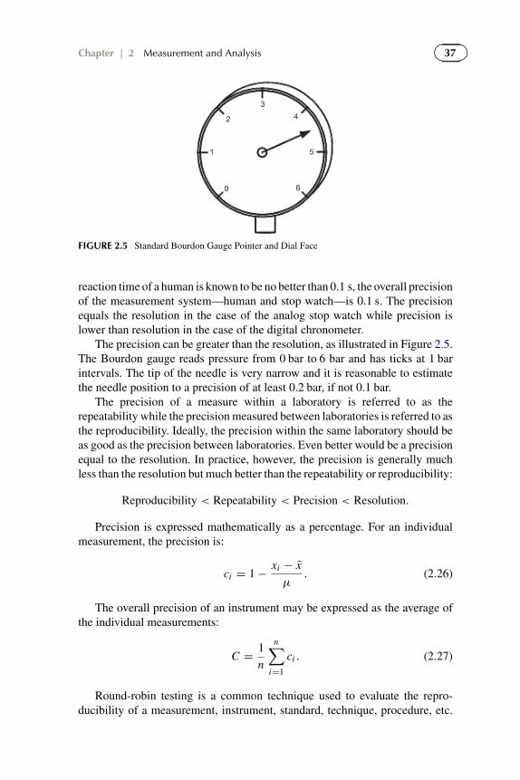
37Chapter | 2 Measurement and Analysis
FIGURE 2.5 Standard Bourdon Gauge Pointer and Dial Face
reaction time of a human is known to be no better than 0.1 s, the overall precisionof the measurement system—human and stop watch—is 0.1 s. The precisionequals the resolution in the case of the analog stop watch while precision islower than resolution in the case of the digital chronometer.
The precision can be greater than the resolution, as illustrated in Figure 2.5.The Bourdon gauge reads pressure from 0 bar to 6 bar and has ticks at 1 barintervals. The tip of the needle is very narrow and it is reasonable to estimatethe needle position to a precision of at least 0.2 bar, if not 0.1 bar.
The precision of a measure within a laboratory is referred to as therepeatability while the precision measured between laboratories is referred to asthe reproducibility. Ideally, the precision within the same laboratory should beas good as the precision between laboratories. Even better would be a precisionequal to the resolution. In practice, however, the precision is generally muchless than the resolution but much better than the repeatability or reproducibility:
Reproducibility < Repeatability < Precision < Resolution.
Precision is expressed mathematically as a percentage. For an individualmeasurement, the precision is:
ci = 1 − xi − x
μ. (2.26)
The overall precision of an instrument may be expressed as the average ofthe individual measurements:
C = 1
n
n∑i=1
ci . (2.27)
Round-robin testing is a common technique used to evaluate the repro-ducibility of a measurement, instrument, standard, technique, procedure, etc.

38 Experimental Methods and Instrumentation for Chemical Engineers
Analytical equipment such as gas chromatographs and especially particle sizedistribution instruments require significant attention to achieve a high level ofreproducibility. For particle size measurements, some chemical plants histori-cally based all measurements on a single instrument and then used these valuesto compare with others—variation between instruments and even technicianswas very high for particle fractions below 44 µm.
2.4.5 Error
Lord Kelvin stated that “to measure is to know” (Unnamed 2011). In fact, itwould be more precise to say that “to measure is to know … better.” Almost allmeasurements have errors with respect to their absolute value, be it temperature,pressure, flow rate, or any of several other standard measurements necessaryto evaluate a phenomenon, characterize an instrument, or run a chemical plant.Error is defined as the absolute or relative difference between the measuredvalue and the true value as measured by a recognized standard. Note that theterm “recognized standard” is mentioned, and not “true value” since the truevalue can rarely, if ever, be known exactly.
For an individual measurement the deviation of the value with respect to thetrue value is expressed by:
di = xi − μ, (2.28)
where xi is an individual measurement and μ is the true value of the mean ofan entire population. When comparing a sample of the population with the truevalue of the mean, error is expressed in the following way:
δ = x − μ. (2.29)
At this point it would be useful to compare the concepts of uncertainty anderror. Error is the difference between the measured value and a standard—the“true value”—while uncertainty is an interval or the range of values withinwhich the true value has a probability to be found. The size of this interval isrelated to the degree of probability defined by the experimenter.
There are three classes of errors: systematic errors are reproducible and thecause is related to some physical law and may be eliminated by appropriatecorrective actions; random errors are unpredictable and irreproducible and canbe characterized by the laws of statistics; finally, inadmissible errors occur asa result of mishandling, incorrect instrument operation, or even poor recordkeeping. Figure 2.6 shows a hierarchical chart that outlines the three types oferrors (Chaouki et al., 2007). Most treatments of error consider systematic andrandom errors. Inadmissible errors might somehow be related to outliers, whichare values that appear to be completely unrelated to a rational data set.
An example of a systematic error would be reading the volume of a graduatedcylinder from the top of the meniscus instead of the bottom. Systematicerrors may also be introduced through improper calibration or changes in the

39Chapter | 2 Measurement and Analysis
Experimental error
Systematic error
Calibration Procedural
Random error
Conditions Interpretation
Inadmissable error
Omission Blunder
FIGURE 2.6 Types of Experimental Error
FIGURE 2.7 Offset and Gain Error
instrument due to use or environmental factors (scale build-up, rust, metalfatigue—localized damage as a result of cyclic loadings—and more).
The zero offset is a common error in measuring pressure with electronictransducers or even typical Bourdon gauges. When the gauge is operated closeto the maximum, a random pressure surge can deform the transducer. The unitmay still be operational (and perhaps give a linear signal) but when the pressureis released the gauge may appear to read a value (either positive or negative).Figure 2.7 demonstrates the zero offset error—at the origin, the reading is greaterthan zero (positive differential). The signal increases linearly with the measuredvariable and it is proportional to the true signal (Patience et al. 2011). Readingthe top of a meniscus to represent volume would be an offset error. A scaleerror (gain error), like the zero offset error, may be caused by an overpressure(or underpressure), mechanical wear, etc. in the case of a pressure transducer.With electronic instruments, it corresponds to the difference between the outputvoltage (or current) at full scale and the calibrated output voltage. A negativegain is illustrated in Figure 2.7.

40 Experimental Methods and Instrumentation for Chemical Engineers
FIGURE 2.8 Instrument Hysteresis
Zero drift represents a variation in the value of the reading with no load asa function of time. A stable instrument maintains the system characteristics forlong periods.
Hysteresis error is the difference between the value of a quantity when it ismeasured going up in scale versus going down in scale, as shown in Figure 2.8.To increase the precision of an instrument that suffers from hysteresis error, themeasurement should always be approached from the same side. This of coursemay not increase accuracy.
Instrument linearity refers to the measurement deviation from an idealstraight-line performance. For instruments that have a nonlinear response, itmust be calibrated along the whole range. The relationship between conductivityand acid concentration is nonlinear: the conductivity increases less thanproportionally with acid concentration (see Figure 2.9).
Errors of omission result from an insufficient rigor in following strictlaboratory protocols. For example, to determine the rate kinetics of a gas-phase reaction, the necessary measurements include composition at the entranceand exit, reactor volume, flow rate, pressure, and temperature. When thereactor is operated at “atmospheric” pressure—that is, the effluent exits tothe atmosphere—the actual operating pressure is invariably different from1.01325 bar. Not only does it depend on the elevation above sea level but also themeteorological conditions. Within hours, the barometric pressure may changeby as much as 5%.
Consider the textile industry and assessing fabric weight (mass per unitarea). It is a parameter used for quality purposes as well as to assess cost. Itwould seem to be a straightforward operation: cut a piece of fabric, calculate itssurface area, and weigh it on a scale. However, procedures have been writtenby many (if not all) standards organizations for this apparently simple test.The procedure is covered in ISO 3801:1977, ASTM D3776:2007, and BS EN

41Chapter | 2 Measurement and Analysis
FIGURE 2.9 Nonlinear Response
12127:1998, to name a few. Measuring the fabric weight essentially considerssix factors:
1. Human factors: The personnel making the measurement should be trainedand qualified;
2. Environmental conditions: The measurement should be made in acontrolled environment maintained at a temperature of (21 ± 2) ◦C and65% relative humidity;
3. Calibration: Experimental instruments must be calibrated—balances,temperature, and relative humidity instruments—on a specified scheduleand a record of the calibration documented;
4. Instrumentation: The measurement must be made with appropriateinstruments—balances, scissors, and rulers;
5. Sampling: The sample of the fabric should come from the center of the roll;6. Conditioning: The sample should be maintained at 21 ◦C and 65% relative
humidity for a period of 24 h before taking the measurement.
The context of a chemical plant is quite different than that of an analyticalor process laboratory: the focus in the laboratory might be to understandthe minimum error allowable to interpret or extrapolate a phenomenon. Thechallenge in the chemical plant is to choose the appropriate measuring intervaland the frequency at which it is measured and stored, how much data is needed,and what precision is necessary to take an action.
The most formidable decision that can be taken in a plant is to initiatean uncontrolled shutdown based on a perceived threat to personnel safety,to the environment, or to equipment integrity. Shutdowns represent a majoreconomic penalty due to lost production but also due to the risk of contaminatingequipment that might require a costly cleanup. Besides operator interventions,automatic triggers are implemented to halt production and bring plants into a

42 Experimental Methods and Instrumentation for Chemical Engineers
stable and safe operating point: interlocks. A high-high (or low-low) interlock isthe most severe trigger and must be carefully set to ensure personnel safety and atthe same time set far enough from standard operating conditions to make sure itwon’t be “accidentally” tripped at a condition that is not particularly hazardous.Temperature and pressure are the two most common interlock triggers. Steelmay be operated at very specific maximum pressures and temperatures, whichare mandated by legislation. In the case of temperature, an interlock might beset at a value of 10–20 ◦C below this value. However, often production ratesmay be increased by increasing temperature and thus in times of high demandthe operating envelope will be increased, thus bringing it closer to the interlocktemperature. Clearly, in this case, the measurement precision must be high inorder to operate with a minimum risk.
Instruments may record chemical plant data at a frequency of severalhundred hertz but storing all these measurements would require enormousdatabases and is both impractical and unnecessary. High frequency data isrecorded and stored temporarily before it is archived in a database managementsystem at a lower frequency—every 15 s is typical. The frequency of thearchived data is increased in the case where variables change suddenly above apredefined threshold value. This threshold value is higher than the resolution ofthe instrument and represents an arbitrary value chosen by the experiencedinstrument engineer. For example, temperature may be recorded at highfrequency with a precision of 0.001 ◦C but generally a precision of ±0.2 ◦C issufficient to monitor a process safely.
2.4.6 Accuracy
An instrument may be precise, but if the measurement deviates from the truevalue, it is inaccurate. Accuracy is a measure of an instrument’s ability toreproduce the true value—it is the degree of closeness to it. It is also known asbias and may be expressed as a fraction or a percentage:
β = 1 − |δ|μ
. (2.30)
In general, accuracy may be improved by increasing sample size—thenumber of measurements. The purpose of calibrating an instrument is to ensurethat the measurement is accurate (Taraldsen 2006, ISO 1995). Calibration willnot improve precision but will reduce the error or increase the exactness.
Figure 2.10 illustrates the difference between accurate precise measure-ments using the target analogy. In Figure 2.10a, the measured values arerandomly off the target, so they are neither accurate nor precise. To improvethe accuracy of the instrument, it must be calibrated and then the values willbecome more evenly distributed around the center, as shown in Figure 2.10b.Calibration will no longer improve the precision: this instrument is accurate butnot precise. Increasing sample size will improve accuracy. In Figure 2.10c, the

43Chapter | 2 Measurement and Analysis
(a) (b) (c) (d)FIGURE 2.10 Accuracy Versus Precision: (a) Imprecise and Inaccurate Measurements; (b)Imprecise but Accurate Measurements; (c) Precise but Inaccurate Measurements; (d) Precise andAccurate Measurements
measured values are close to each other in one area of the target. In this case, themeasurements are precise but they are inaccurate. Calibration would improvethe accuracy of the instrument. Finally, in Figure 2.10d, the measurements areboth precise and accurate: all measurements are close together and clusteredaround the target value.
Example 2.7. The accuracy written on the side of the Erlenmeyer flask ofExample 2.1 was 5%, while it was 1.4 ml for the graduated cylinder and only0.08 ml for the volumetric flask.
(a) What is the precision and accuracy of each?(b) How do these values compare with the reported accuracy and the standard
deviation?(c) How would the accuracy and precision change if you were to read in between
the graduation marks of the Erlenmeyer flask at a value of 110 ml?
Solution 2.7a. To calculate the accuracy, first the error of each sample must becalculated: �1 = 100 ml − 99.69 ml = 0.31 ml, �2 = 100 ml − 97.89 ml =2.11 ml, �3 = 100 ml − 103.47 ml = 3.47 ml.
Together with the absolute error and the true value of the mean, the accuracyis determined from the following expression:
βi = 1 − |δ|μi
,
resulting in β1 = 99.69%, β2 = 97.9%, and β3 = 96.5%.The overall precision of each measuring vessel is determined by calculating
the difference between the values of the individual measurements and the samplemean:
ci = 1 − |xi − x |μ
.

44 Experimental Methods and Instrumentation for Chemical Engineers
The average of these values gives the overall precision:
Ci = 1
n
n∑j=1
ci, j
with C1 = 99.95%, C2 = 99.73%, and C3 = 99.47%.In terms of volume, the precision of each vessel is C1 = 0.05 ml, C2 =
0.27 ml, and C3 = 0.53 ml.
Solution 2.7b. The precision of all measuring devices is close to an order ofmagnitude higher than the accuracy. The precision is lower than the standarddeviation on average by 75%.
Solution 2.7c. Both the accuracy and the precision of the Erlenmeyer flask arebetter than expected because the volume was measured at a graduation mark.Moving away from the graduation mark would decrease both the accuracy andprecision because of a lack of reference with which to assess the volume in aconsistent manner.
2.4.7 Repeatability and Reproducibility
Both the concepts of repeatability and reproducibility are related to accuracy:repeatability is defined as “the closeness of agreement between the results ofsuccessive measurements of the same measurand carried out subject to all ofthe following conditions: the same measurement procedure, the same observer,the measuring instrument used under the same conditions, the same location,and repetition over a short period of time.” The definition of reproducibility is:“the closeness of agreement between the results of measurements of the samemeasurand, where the measurements are carried out under changed conditionssuch as: different principles or methods of measurement, different observers,different measuring instruments, different locations, different conditions of use,or different periods of time.”
The basics of inter-laboratory (between laboratories) and intra-laboratory(within a laboratory) studies have been summarized in the ISO-5725 standard(Feinberg 1995). Recognizing that measurements are often laborious toundertake, examples cited in the standard have often only three measurementsper test and only four laboratories. A single reported measurand, y, is the sumof the true value, x, a component of the accuracy, B, and a component of randomvariability during any measurement, e (within the laboratory variance):
y = x + B + e. (2.31)
Figure 2.11 illustrates the inter-laboratory variance, s2L , at the top and
the intra-laboratory variance, s2r —the repeatability variance—, at the bottom,
which is much narrower. Assuming equality of variance for each laboratory

45Chapter | 2 Measurement and Analysis
FIGURE 2.11 Intra- and Inter-Laboratory Variance
participating in an inter-laboratory study, the repeatability variance is equal tothe mean of the repeatability variance of each laboratory:
s2r = 1
n
n∑i=1
s2r ,i . (2.32)
The inter-laboratory variance is calculated based on the variance of themeans of the individual laboratories, where xi is the mean of each individuallaboratory and xL is the mean of the value of the means of the laboratories.However, the intra-laboratory variance includes part of the repeatabilityvariance that must be subtracted out (the second term of the left-hand side):
s2L = 1
n − 1
n∑i=1
(xi − xL)2 − s2r
n. (2.33)
The reproducibility variance, s2R , equals the sum of the intra-laboratory
variance and the inter-laboratory variance:
s2R = s2
L + s2r , (2.34)

46 Experimental Methods and Instrumentation for Chemical Engineers
from which the reproducibility standard deviation is calculated:
sR =√
s2L + s2
r . (2.35)
Example 2.8. An international program has been undertaken to develop amosquito repellent based on nepetalactone (NPL). A sample has been preparedto share between three laboratories to be analyzed by gas chromatography. Themeasurements (in mol%) of the first laboratory were 73.8, 71.4, 77.2, and 76.0;those of the second were 69.3, 72.1, 74.3, and 65.5; and those of the third were74.9, 76.3, 73.7, and 73.0. Calculate the standard deviation of repeatability andreproducibility for the study.
Solution 2.8. The mean and variance for each laboratory are calculated:x1 = 74.6, s2
1 = 6.5, x2 = 70.3, s22 = 14.4, x3 = 74.6, s2
3 = 2.1.The repeatability variance equals the mean of the individual variances of eachlaboratory: s2
r = 1n
∑ni=1 s2
r ,i = 7.7, sr = 2.8 mol%.The inter-laboratory variance is derived from the variance of the mean values ofeach laboratory subtracted by the repeatability variance divided by the numberof degrees of freedom:
s2L = 1
n − 1
n∑i=1
(xi − xL)2 − s2r
n= 12.3 − 7.7
3= 9.7
The reproducibility variance is the sum of the repeatability variance and theinter-laboratory variance: s2
R = s2r + s2
L = 7.7 + 8.7 = 17.4, sR = 4.2.Thus the standard deviation of repeatability, sR , equals 1.6 mol% and that ofreproducibility, SR , is 4.2 mol%.
A more rigorous definition of repeatability has been described in the DIN 1319standard. According to this definition, data is measured at the full-scale readingof the instrument and then reduced to 50% of full scale and measured again.This procedure is repeated for a total of 10 measurements each. The mean valuesat 100% FS and 50% FS are calculated:
X50% = 1
n
n∑i=1
Xi,50%,
X100% = 1
n
n∑i=1
Xi,100%.
47Chapter | 2 Measurement and Analysis
The relative standard deviations at 50% FS and 100% FS are:
Srel,50% = 1
X100% − X50%
√√√√ 1
n − 1
n∑i=1
(Xi,50% − X50%)2,
Srel,100% = 1
X100% − X50%
√√√√ 1
n − 1
n∑i=1
(Xi,100% − X100%)2.
2.5 REPRESENTING DATA GRAPHICALLY
Graphs are an efficient means to identify trends, establish relationships, andevaluate the extent of errors or outliers. They are powerful tools to communicateideas and concepts. The scales on the abscissa and ordinate are generallyselected to cover the whole range of the data—from the origin to the maximumof the experimental data. By expanding the scales to fit the entire data range,the variation in the data becomes more evident.
Scatter plots are the most common type of graph used to show relationshipsbetween a dependent variable (responses) and independent variables (factors).Judiciously selecting and sizing the symbols in scatter plots allows one tocommunicate trends and the measured values’ associated error. Frequently, toshow the effect of more than one independent variable, different symbol typesor colors can be used. Three-dimensional plots, surface plots, and contour plotsare becoming more common to illustrate the effect of two or more factors on thedependent variable. Bar charts (and pie charts) are popular for presentations, andhistograms are useful to compare the distribution of populations. Ternary plotsare used in thermodynamics and to demonstrate explosion limits of differentcompositions of gases.
Plotting experimental data on ordinary rectangular coordinates is the firststep to assess the quality of the data as well as to begin to understand therelationship between dependent variables and factors. Figure 2.12 illustratesthe trend of the pressure drop as a function of volumetric flow rate of oxygenthrough multiple nozzles entering a reactor. It is clear that due to the curvaturein the data a simple linear relationship is inapplicable. The shape of the curveis typical of a power law function that passes through the origin: the pressuredrop equals zero when there is no flow.
Q �= a�P + b. (2.36)
The next step is to plot the data on logarithmic scales for both the abscissaand ordinate as in Figure 2.13 (known as a log-log plot). A standard conventionis that experimental data should be represented by symbols while correlationsand models should be represented by lines. The plant data shows significantscatter at low volumetric flow rates but from approximately 1 m3 h−1 and

48 Experimental Methods and Instrumentation for Chemical Engineers
FIGURE 2.12 Linear Plot of Volumetric Flow Rate Versus Pressure Drop
FIGURE 2.13 Log-Log Plot of Nozzle Volumetric Flow Rate Versus Pressure Drop
beyond, the data falls on a straight line. The slope of the line corresponds tothe exponent. The concave down shape indicates that the exponent is less than1 (and that the first derivative is negative) while a concave up shape wouldindicate an exponent greater than 1 (and a positive first derivative).
Q = a�Pn . (2.37)
The scatter in the data at the lower end may be a result of perturbationsduring start-up and shut-down, instrument error, or it may simply mean thatthe plant is out of the range of standard operation. Later, we will discuss underwhat conditions experimental measurements may be ignored.
Models should normally be included in a figure whenever possible. Often,lines may be introduced in a figure to demonstrate tendencies more clearly—trend lines—but they do not represent a physical phenomenon. In the case of

49Chapter | 2 Measurement and Analysis
FIGURE 2.14 Butane Conversion Versus Contact Time
the pressure drop, when the exponent n equals 0.5, the volumetric flow rateincreases with the square root of the pressure drop. This relationship agreeswith orifice theory that relates the volumetric flow rate (Q), to pressure drop(�P), density (ρ), cross-sectional area (X A), and the ratio of orifice diameterto pipe diameter (β):
Q = 0.61X A√
1 − β4
√2�P
ρ. (2.38)
Another exponential relationship common to reactor engineering is thatbetween conversion and the ratio of the reactor (or catalyst) volume, V, andthe volumetric flow rate, Q. This ratio is referred to as the contact time, τ .Maleic anhydride (MA) is an important chemical intermediate that is formedby the partial oxidation of butane over a vanadium pyrophosphate. Figure 2.14plots n-butane conversion, X, against contact time, τ—collected in an idealmicro-reactor on ordinary rectangular co-ordinates. Since the shape of the datais concave down, we might assume that the relationship is a power law with anegative exponent. However, the data points do not fall on the trend line drawnin Figure 2.15.
In this case, we may be tempted to assume that the data has experimentalerror and simply calculate the slope of the line. Changing the scales of theordinate and abscissa can squeeze the data together, enforcing a tendency toreject the possibility of a different functional relationship. However, in the caseof an ideal reactor in which conversion is independent of the concentrationof the reactants, the differential equation relating the conversion to theconditions is:
Qd X
dV= −k(1 − X), (2.39)
where k is the first-order rate constant. The solution to this equation gives anexponential function. The value of the rate constant that best fits the data is

50 Experimental Methods and Instrumentation for Chemical Engineers
FIGURE 2.15 Log-Log Plot of n-Butane Conversion Versus Contact Time
�
�
�
�
TABLE 2.4 Graphical Transformations Commonly Used to Linearize Data
y = a + bxn In this case, the y intercept is first determined(graphically) and then a log-log plot of y−a versusx will give a straight line with slope equal to n
y = a + bx The dependent variable, y , is simply plotted as a
function of the inverse of the dependent variable.Rate constants of chemical reactions follow anArrhenius-type expression, k = A exp
(− Ea
RT
). A
plot of ln k versus 1T gives a straight line with slope
equal to − EaR
y = abx This should be linearized by plotting ln y versus x
0.3 s−1. The agreement between the experimental data and this model is good,as demonstrated in Figure 2.14.
X = 1 − e−kτ . (2.40)
Other graphical transformations that can be used to linearize data are shown inTable 2.4.
Figure 2.16 shows the trend of selectivity versus conversion for thepartial oxidation of n-butane to maleic anhydride in a fluidized bed reactor.Besides the by product acids (acrylic and acetic), CO and CO2 are the principalproducts either formed directly from butane (parallel reaction) or via maleic

51Chapter | 2 Measurement and Analysis
FIGURE 2.16 MA Selectivity Versus n-C4H10 Conversion
anhydride (series reaction):
C4H10 + 7
2O2→C4H2O3 + 4H2O,
C4H10 + 11
2O2→2CO2 + 2CO + 5H2O,
C4H2O3 + 2O2→2CO2 + 2CO + H2O.
The range of conversion varies from about 5% to almost 80% and theselectivity is greater than 20% but less than 80%. The scale was chosen torepresent the absolute limits of conversion and selectivity possible. They couldalso have been chosen to span only the range of the data, as shown in Figure 2.13and Figure 2.14.
In Figure 2.17, the symbols of all collected data at 350 ◦C are circular andblack. The symbols of the 380 ◦C data are red inverted triangles while the400 ◦C data is represented by green squares. When figures are reproduced inblack and white, the difference between white (or “empty”) and black symbolsis clearly obvious but even colors appear as different shades of gray. Usingdifferent colors and shapes ensures that the differences between separate sets ofdata are distinguishable. This graph shows that selectivity is highest at 350 ◦Cand the lowest selectivity is at 410 ◦C—more information is communicated byadding color and shapes compared to Figure 2.16.
The third graph of the same data, Figure 2.18, is plotted to highlight theeffect of changing feed concentrations (mol% or vol%) of butane and oxygen.The experiments were conducted with six combinations from low butane andoxygen (2% and 4%, respectively) to high butane and oxygen concentrations(9% and 10%, respectively). Again, independent symbols and colors wereadopted for each condition. All symbols were outlined with a black edge forclarity. The trends in the data set become more obvious by plotting the data
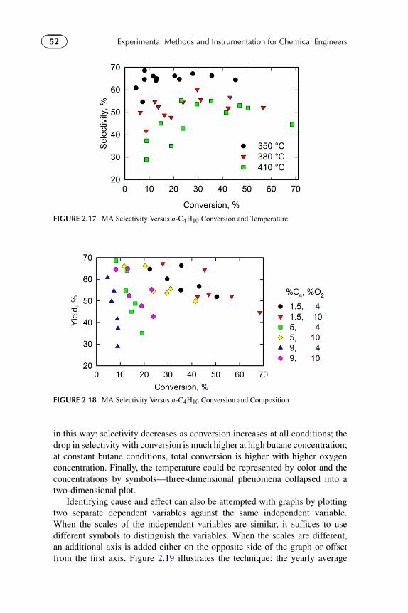
52 Experimental Methods and Instrumentation for Chemical Engineers
FIGURE 2.17 MA Selectivity Versus n-C4H10 Conversion and Temperature
FIGURE 2.18 MA Selectivity Versus n-C4H10 Conversion and Composition
in this way: selectivity decreases as conversion increases at all conditions; thedrop in selectivity with conversion is much higher at high butane concentration;at constant butane conditions, total conversion is higher with higher oxygenconcentration. Finally, the temperature could be represented by color and theconcentrations by symbols—three-dimensional phenomena collapsed into atwo-dimensional plot.
Identifying cause and effect can also be attempted with graphs by plottingtwo separate dependent variables against the same independent variable.When the scales of the independent variables are similar, it suffices to usedifferent symbols to distinguish the variables. When the scales are different,an additional axis is added either on the opposite side of the graph or offsetfrom the first axis. Figure 2.19 illustrates the technique: the yearly average

53Chapter | 2 Measurement and Analysis
FIGURE 2.19 Global CO2 Concentration and Local Temperature Versus Time
local temperature in Montreal, Canada (Environnement Canada 2011) is plottedcoincidentally with the atmospheric CO2 concentration (in ppm) as recorded atthe Mauna Loa observatory in Hawaii (Keeling and Whorf 1999).
Global warming has attracted significant interest in scientific literature, forboth government policy makers and the general public. It is commonly heldthat greenhouse gases (GHG), particularly CO2, are a major contributor toa measurable increase in the average world temperature. A plot of averagetemperature and CO2 concentration should demonstrate a similar rising trend.In North America, meteorological stations record local temperatures every hour.A yearly average consists of almost 9000 readings. The left ordinate representsthe concentration of CO2, the right ordinate depicts the average temperaturewhile the abscissa is time. Whereas over the 50-yr period starting in 1959 theCO2 concentration has steadily risen from below 320 ppm to over 380 ppm—a 21% increase—the average temperature varies between 4.6 ◦C in 1980 and8.6 ◦C in 2006. The five highest temperatures were recorded between 1998 and2006 but between 1959 and 2006, when the CO2 concentration rose by 40 ppm,the temperature would appear to have been constant. In fact, from the mid-1950sup until the 1980s, the temperature arguably decreased.
2.5.1 Plotting Pitfalls
When plotting data, the extremes of the axes should be chosen so that theindependent and dependent variables just fit within the graph. Choosing largervalues for the axes’ extremes will compress the data and give the appearance oflinearity where none might exist. Another common error is to plot a variable thatis itself a multiple of the factor being plotted. This will linearize the functionand will again lead to a false impression with respect to the phenomenon.
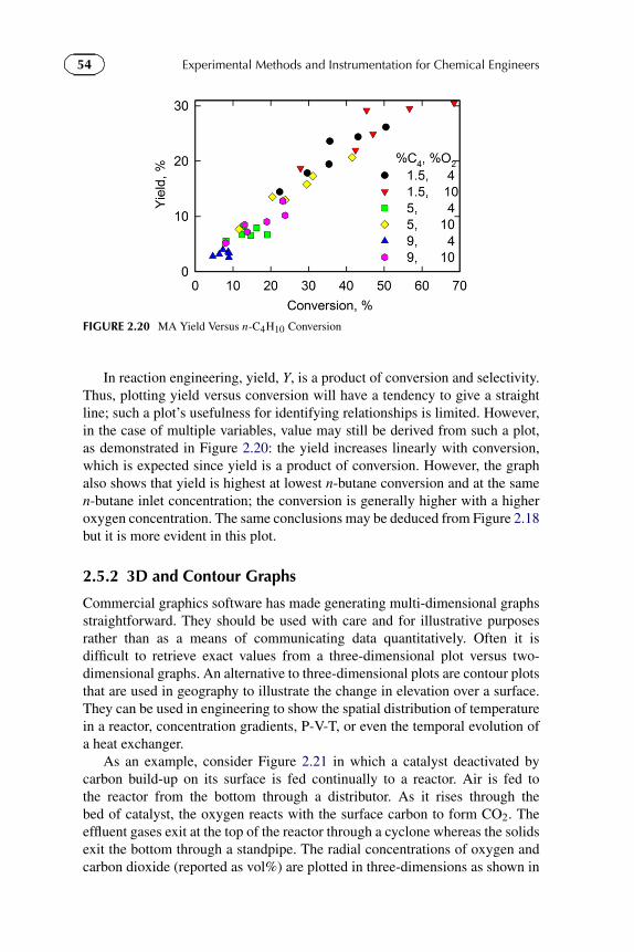
54 Experimental Methods and Instrumentation for Chemical Engineers
FIGURE 2.20 MA Yield Versus n-C4H10 Conversion
In reaction engineering, yield, Y, is a product of conversion and selectivity.Thus, plotting yield versus conversion will have a tendency to give a straightline; such a plot’s usefulness for identifying relationships is limited. However,in the case of multiple variables, value may still be derived from such a plot,as demonstrated in Figure 2.20: the yield increases linearly with conversion,which is expected since yield is a product of conversion. However, the graphalso shows that yield is highest at lowest n-butane conversion and at the samen-butane inlet concentration; the conversion is generally higher with a higheroxygen concentration. The same conclusions may be deduced from Figure 2.18but it is more evident in this plot.
2.5.2 3D and Contour Graphs
Commercial graphics software has made generating multi-dimensional graphsstraightforward. They should be used with care and for illustrative purposesrather than as a means of communicating data quantitatively. Often it isdifficult to retrieve exact values from a three-dimensional plot versus two-dimensional graphs. An alternative to three-dimensional plots are contour plotsthat are used in geography to illustrate the change in elevation over a surface.They can be used in engineering to show the spatial distribution of temperaturein a reactor, concentration gradients, P-V-T, or even the temporal evolution ofa heat exchanger.
As an example, consider Figure 2.21 in which a catalyst deactivated bycarbon build-up on its surface is fed continually to a reactor. Air is fed tothe reactor from the bottom through a distributor. As it rises through thebed of catalyst, the oxygen reacts with the surface carbon to form CO2. Theeffluent gases exit at the top of the reactor through a cyclone whereas the solidsexit the bottom through a standpipe. The radial concentrations of oxygen andcarbon dioxide (reported as vol%) are plotted in three-dimensions as shown in

55Chapter | 2 Measurement and Analysis
GasDistributor
Solids’Exit
ExhaustGas
Cyclone
Solids’Entry
FIGURE 2.21 Fluidized Bed Regenerator
FIGURE 2.22 3D Plot of Oxygen Distribution Across a 4 m Diameter Regenerator (For colorversion of this figure, please refer the color plate section at the end of the book.)
Figures 2.22 and 2.23, respectively. The oxygen concentration is lowest in thecenter of the reactor parallel to the solids entry point and is highest on bothsides perpendicular to the entry point. Figure 2.23 shows the variation of the
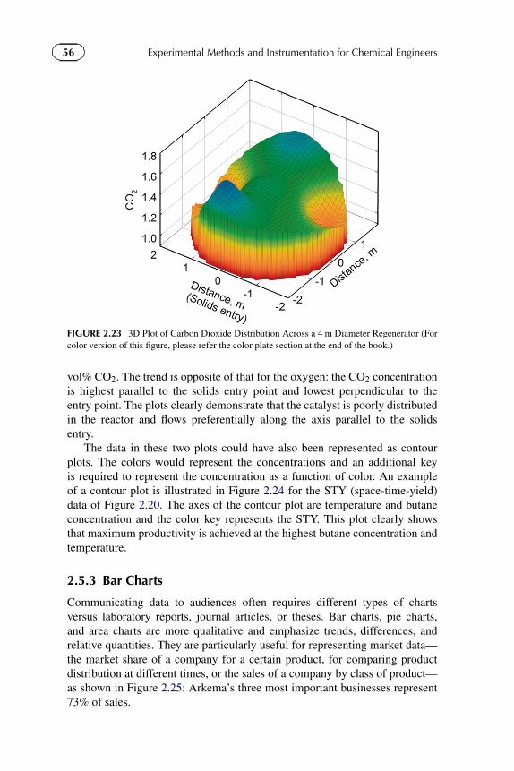
56 Experimental Methods and Instrumentation for Chemical Engineers
FIGURE 2.23 3D Plot of Carbon Dioxide Distribution Across a 4 m Diameter Regenerator (Forcolor version of this figure, please refer the color plate section at the end of the book.)
vol% CO2. The trend is opposite of that for the oxygen: the CO2 concentrationis highest parallel to the solids entry point and lowest perpendicular to theentry point. The plots clearly demonstrate that the catalyst is poorly distributedin the reactor and flows preferentially along the axis parallel to the solidsentry.
The data in these two plots could have also been represented as contourplots. The colors would represent the concentrations and an additional keyis required to represent the concentration as a function of color. An exampleof a contour plot is illustrated in Figure 2.24 for the STY (space-time-yield)data of Figure 2.20. The axes of the contour plot are temperature and butaneconcentration and the color key represents the STY. This plot clearly showsthat maximum productivity is achieved at the highest butane concentration andtemperature.
2.5.3 Bar Charts
Communicating data to audiences often requires different types of chartsversus laboratory reports, journal articles, or theses. Bar charts, pie charts,and area charts are more qualitative and emphasize trends, differences, andrelative quantities. They are particularly useful for representing market data—the market share of a company for a certain product, for comparing productdistribution at different times, or the sales of a company by class of product—as shown in Figure 2.25: Arkema’s three most important businesses represent73% of sales.
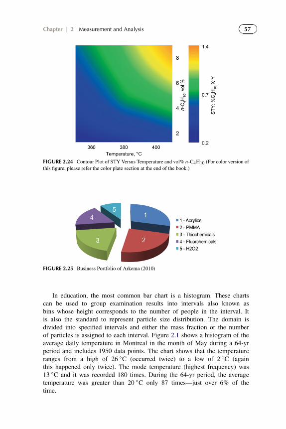
57Chapter | 2 Measurement and Analysis
FIGURE 2.24 Contour Plot of STY Versus Temperature and vol% n-C4H10 (For color version ofthis figure, please refer the color plate section at the end of the book.)
FIGURE 2.25 Business Portfolio of Arkema (2010)
In education, the most common bar chart is a histogram. These chartscan be used to group examination results into intervals also known asbins whose height corresponds to the number of people in the interval. Itis also the standard to represent particle size distribution. The domain isdivided into specified intervals and either the mass fraction or the numberof particles is assigned to each interval. Figure 2.1 shows a histogram of theaverage daily temperature in Montreal in the month of May during a 64-yrperiod and includes 1950 data points. The chart shows that the temperatureranges from a high of 26 ◦C (occurred twice) to a low of 2 ◦C (againthis happened only twice). The mode temperature (highest frequency) was13 ◦C and it was recorded 180 times. During the 64-yr period, the averagetemperature was greater than 20 ◦C only 87 times—just over 6% of thetime.

58 Experimental Methods and Instrumentation for Chemical Engineers
2.6 FAST FOURIER TRANSFORM (FFT)
Whereas the data in Figure 2.1 is distributed essentially evenly around themean, there are instances where data repeats at certain intervals or at a certainfrequency. For reciprocating equipment—compressors, pumps, blowers, etc.—the pressure downstream will typically vary with the period of rotation. Anotherexample is heart rate: the heart beats at a regular frequency that may varydepending on the time of day—morning or evening—or the exertion at a givenmoment. When diagnosing problems in equipment or in a patient, it is useful torecord the data and then analyze the characteristic frequencies to help identifyany problem that might exist.
Figure 2.26 plots the voltage as measured by a cardiogram versus time fora healthy patient—the voltage increases at regular intervals. At a frequencyof 1 Hz, the curve repeats. Deriving conclusions from data plotted in the time
FIGURE 2.26 Cardiogram
FIGURE 2.27 Cardiogram FFT

59Chapter | 2 Measurement and Analysis
domain is difficult. Rather, the data may be compared in the frequency domainto identify anomalies. Figure 2.27 is a graph of the power, as calculated byFFT, versus the frequency. The peaks represent the dominant frequencies.By measuring the heart rate at different parts of the body and comparingtheir signals, cardiac diseases may be detected. Moreover, if the FFT hasmultiple peaks (beyond the standard for a healthy individual), that would alsobe indicative of heart disease.
2.7 EXERCISES
2.1 Calculate the numerical value of each operation, taking into account thenumber of significant figures.
(a) (5.2 × 10−4 · 1.635 × 106)/2.67 .(b) 3.57 · 4.286 .(c) 1530 − 2.56 .(d) 0.036 + 0.22 .
2.2 The mass of a single application of mosquito repellent is determinedby spraying a tissue and subtracting the tare weight of the tissue fromthe total weight measured in a precision balance. The tissue is weighedimmediately after spraying to minimize mass loss due to evaporation.The mass of a single pump action of a mosquito repellent was measured10 times (in g): 0.1155, 0.1192, 0.1106, 0.1137, 0.1075, 0.1158, 0.1076,0.0982, 0.1028, and 0.108.
(a) Calculate the average, variance, and standard deviation.(b) If the true value of the mass of a single application (spraying
once) is 0.1140 g, calculate the absolute and relative error of eachmeasurement.
(c) What is the sensitivity of the instrument?(d) Calculate the standard deviation of the error.(e) Comment on the reproducibility and the accuracy of the
measurements.
2.3 According to the Chauvenet criterion, could we reject one of the followingexperimental points: 32, 34, 25, 33, 37, and 10? Calculate μ,σ , and α.Calculate the value of P.
2.4 To increase the precision of the measurement of the mass of a singleapplication of mosquito repellent, the spray is directed toward analuminum boat, which is weighed after the 10th consecutive spray. Theresults after 10 runs (in g) are: 1.1516, 1.1385, 1.141, 1.1391, 1.1385,1.148, 1.1271, 1.1354, 1.1439, and 1.1153.
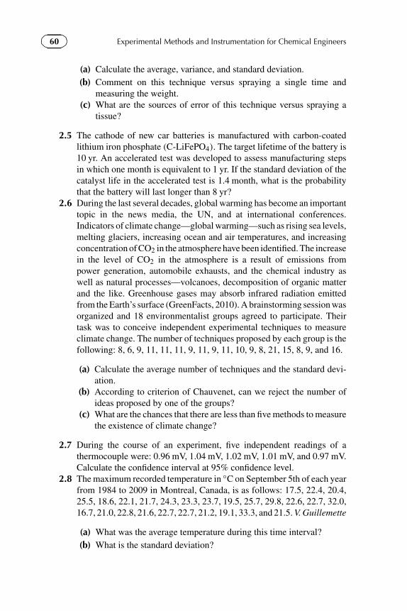
60 Experimental Methods and Instrumentation for Chemical Engineers
(a) Calculate the average, variance, and standard deviation.(b) Comment on this technique versus spraying a single time and
measuring the weight.(c) What are the sources of error of this technique versus spraying a
tissue?
2.5 The cathode of new car batteries is manufactured with carbon-coatedlithium iron phosphate (C-LiFePO4). The target lifetime of the battery is10 yr. An accelerated test was developed to assess manufacturing stepsin which one month is equivalent to 1 yr. If the standard deviation of thecatalyst life in the accelerated test is 1.4 month, what is the probabilitythat the battery will last longer than 8 yr?
2.6 During the last several decades, global warming has become an importanttopic in the news media, the UN, and at international conferences.Indicators of climate change—global warming—such as rising sea levels,melting glaciers, increasing ocean and air temperatures, and increasingconcentration of CO2 in the atmosphere have been identified. The increasein the level of CO2 in the atmosphere is a result of emissions frompower generation, automobile exhausts, and the chemical industry aswell as natural processes—volcanoes, decomposition of organic matterand the like. Greenhouse gases may absorb infrared radiation emittedfrom the Earth’s surface (GreenFacts, 2010). A brainstorming session wasorganized and 18 environmentalist groups agreed to participate. Theirtask was to conceive independent experimental techniques to measureclimate change. The number of techniques proposed by each group is thefollowing: 8, 6, 9, 11, 11, 11, 9, 11, 9, 11, 10, 9, 8, 21, 15, 8, 9, and 16.
(a) Calculate the average number of techniques and the standard devi-ation.
(b) According to criterion of Chauvenet, can we reject the number ofideas proposed by one of the groups?
(c) What are the chances that there are less than five methods to measurethe existence of climate change?
2.7 During the course of an experiment, five independent readings of athermocouple were: 0.96 mV, 1.04 mV, 1.02 mV, 1.01 mV, and 0.97 mV.Calculate the confidence interval at 95% confidence level.
2.8 The maximum recorded temperature in ◦C on September 5th of each yearfrom 1984 to 2009 in Montreal, Canada, is as follows: 17.5, 22.4, 20.4,25.5, 18.6, 22.1, 21.7, 24.3, 23.3, 23.7, 19.5, 25.7, 29.8, 22.6, 22.7, 32.0,16.7, 21.0, 22.8, 21.6, 22.7, 22.7, 21.2, 19.1, 33.3, and 21.5. V. Guillemette
(a) What was the average temperature during this time interval?(b) What is the standard deviation?

61Chapter | 2 Measurement and Analysis
(c) What is the likelihood that the temperature drops below 20 ◦C?(d) According to the criterion of Chauvenet, can we reject some of the
values for the temperature?(e) Is there a statistical trend in the data (any evidence of climate
change)?
2.9 A pharmaceutical company requires a ventilation system to purify theair of a biohazard containment laboratory. HEPA, ULPA, and SULPAtechnologies were considered but the ULPA filters were deemed sufficientfor the particle size of the likely contaminants. The life span (in days) ofthe air filter given by the different suppliers is: 80, 110, 100, 150, 170,60, 90, 90, 80, 110, 90, 110, 80, 90, 160, 110, 90, 210, 160, 120, 110, and110. A. R. Nassani
(a) What are the average life, variance, and standard deviation of thefilters?
(b) Based on the criterion of Chauvenet, are all of the life spans claimedby the suppliers credible?
2.10 Differential pressure in vessels and pipes containing gases is oftenmeasured with U-tube manometers. The difference in pressure from onepoint to another is proportional to the difference in height between thevertical legs of the manometer:
�P = (ρmano − ρfluid)g�H ,
where ρmano is the density of the fluid in the gauge and ρfluid is the densityof the fluid in the vessel or pipe. Often, ρmano � ρfluid and thus ρfluidmay be neglected. Six measurements were recorded for air near STP witha U-tube: 0.154, 0.146, 0.149, 0.161, 0.152, and 0.144. The manometerfluid has a density of 830 kg m−3. N. Fadlallah
(a) Calculate average pressure drop, variance, and standard deviation.(b) Determine the confidence interval at a 99% confidence level.(c) What is the uncertainty in the calculated pressure differential?
2.11 During a trek in the mountains, you feel lightheaded and presume it is dueto lack of oxygen. Based on an altimeter reading, you are at an elevationof (2750±50) m above sea level. Calculate the partial pressure of oxygenand the uncertainty. The relationship between pressure and elevation (Zin m) is given by:
P = Po(1 − 2.255 × 10⁻⁵ Z)5.255.

62 Experimental Methods and Instrumentation for Chemical Engineers
2.12 Your laboratory is responsible for the development of a submersible todetect oil leaks at a maximum pressure of 250 MPa. You estimate thedensity of sea water as (1030 ± 15) kg m−3 and that your depth gaugeis accurate to ±1.00% at a full-scale reading of 300 MPa.
(a) What is the maximum allowable depth at a 95% confidence levelthat you recommend for standard operation?
(b) What is the maximum allowable depth at a 99% confidence level?
2.13 Solvent tanks must be purged prior to maintenance operations to ensurethat the level of oxygen is sufficient and that the vapor concentration isbelow the flash point and the limit authorized by OHSA (OccupationalSafety and Health Association)—(500 ± 5) ppm. The volume of eachtank is (8.0 ± 0.3) m3, all liquid was drained beforehand, and the vaporis initially saturated. G. Alcantara
Determine the time and uncertainty needed to purge each tank toreach the maximum permitted by OSHA on the basis that the purge rateis (2.00 ± 0.05) m3 m−1 at a pressure of 0.1 MPa and a temperature of22 ◦C. Use the following expression:
yi,final = yi,initial exp
(− Vpurge
Vreservoirt
).
2.14 Five equations to correlate the molar heat capacity (C p—J mol−1 K−1)as a function of temperature are given in Section 2.2.
(a) Assuming that one of the equations is correct, calculate the errorbetween this value and values predicted by the other correlations at0 ◦C, 100 ◦C, 1000 ◦C, and 2000 ◦C.
(b) The fitted constants in the NIST equations carry seven significantfigures. What is the error at 0 ◦C, 100 ◦C, 1000 ◦C, and 2000 ◦Cwith only six, five, and four significant figures?
2.15 A student must carry out a chemical engineering laboratory test featuringthe following reaction: A + B → C. For this reaction to take place, hemust boil the reagents. He collects 20 ml of A and B with a volumetricpipette of 20 ml (its uncertainty is 0.03 ml). After bringing the mixture to aboil, the student collects the product in a graduated cylinder. The reactionis complete (no reactants are left over). The experimental volume of Cis 48.5 ml (the uncertainty of the specimen is 0.5 ml). The density of Cis 0.825 kg l−1, its molecular mass is 28.0 g mol−1, and the theoreticalmolar yield is 1.50 mol. S. Deacken
(a) Calculate the theoretical volume of C.(b) Calculate the relative error of the volume.(c) Calculate the relative uncertainty of the experimental volume.(d) Describe what kinds of errors could have been committed.

63Chapter | 2 Measurement and Analysis
2.16 Calculate the molecular mass of air, assuming a relative humidity of 0%.The molar composition equals: 21.0% O2, 78.1% N2, and 0.9% Ar.
2.17 Nube wishes to purchase a laptop. His single criterion is the lifetimeof its battery. He compares the battery lifetimes of 15 of his colleaguespossessing a laptop and obtains the following results (in min): 182, 130,167, 198, 145, 156, 165, 181, 176, 120, 90, 123, 179, 201, and 137. M.Brière-Provencher
(a) What are the average, the standard deviation, and the variance of thebatteries’ lifetimes?
(b) What is the probability that Nube’s computer will operate for over170 min if the samples respect a normal distribution?
(c) Determine if data can be eliminated by applying Chauvenet’scriterion.
2.18 As of 2005, the maximum permissible concentration of sulfur in gasolineis 30 ppm. Table Q2.18 summarizes the measured sulfur content for threegrades of fuel in 2001—before the new regulations—and in 2005. É.Michaud
(a) The units of parts per million (ppm) are 10−6 g m−3. Comparethe concentration of sulfur in gasoline permitted by law versusthe measured values in 2001 and 2005. Express the differences inabsolute and relative concentrations. Comment.
(b) What is the 95% confidence interval for both ordinary and superfuels in 2001 and 2005?
�
�
�
�
TABLE Q2.18 Sulfur in Liquid Fuels (wt % Sulfur)
2001Ordinary 0.028 0.038 0.029 0.025
Super 0.020 0.019 0.011 0.011
Aviation <0.001 <0.001 <0.002 <0.001
2005Ordinary 0.0018 0.0021 0.0026 0.0022
Super 0.0001 0.0002 0.0001 0.0002
Aviation <0.0001 <0.0001 <0.0001 <0.0001
2.19 At high shear rates, the viscosity of a polymer melt behaves like a powerlaw fluid characterized by the Carreau equation:
η = ηo(1 + λ2γ )(β−1)/2,

64 Experimental Methods and Instrumentation for Chemical Engineers
F= 100 kmol/h
z=0.5
L
V = 70 kmol/hy = ?
FIGURE Q2.20 Flash Separation
where ηo is the consistency index (25 ± 1) mPa s, λ is the characteristictime of fluid 4 s ±10%,β is the rheo-plasticizer index (0.72±0.05), andγ is the shear rate (s−1).
Calculate the polymer melt’s viscosity and uncertainty at a shear rateof 0.112 s−1. E. Nguyen
2.20 A mixture of benzene and toluene (50 ± 1%) is fed to an evaporator ata rate of 100 kmol h−1, as shown in Figure Q2.20. The vapor effluentstream is 70 kmol h−1. The uncertainty of each flow rate is 1%. Thevapor-liquid equilibrium constant equals 1.78. Determine the fraction ofbenzene in the vapor phase and the uncertainty. The fraction of benzenein the vapour phase maybe calculated from the formula: L.-D. Lafond
y = Fz
V + L/K.
2.21 A student who struggles to arrive on time for his first class in the morningdecides to make a statistical study of the time it takes to travel to school onrollerblades. After 10 consecutive days of measurement, his results were:58′39′′, 56′43′′, 59′32′′, 52′36′′, 54′42′′, 56′37′′, 57′25′′, 58′36′′, 54′39′′,and 52′27′′. How long before his class starts should he leave the house toarrive on time 90% of the time? J.-S. Boisvert
2.22 HadCRUT32 is a record of global temperatures that spans 160 yr andis compiled from both land measurements (Climate Research Unit—CRU—of the University of Anglia) and sea surface measurements(Hadley Center). Figure Q2.22 shows the temperature data together withthe atmospheric CO2 measurements collected at Mauna Loa.
2 http://www.cru.uea.ac.uk/cru/data/temperature/hadcrut3gl.txt

65Chapter | 2 Measurement and Analysis
FIGURE Q2.22 HadCRUT3 Average Global Temperature
(a) Does the change in CO2 concentration correlate with the rise inglobal temperature? Discuss.
(b) How is the temperature data different from that reported in Figure2.19?
(c) What are the likely sources of error of the HadCRUT3 temperaturedata?
(d) The following equation characterizes the rise in CO2 concentrationin the atmosphere as reported by the Mauna Loa observatory:
ppmCO2= 316 + 0.38(t − 1958)4/3,
where t is the calendar time (yr). What was the rate at which CO2accumulated in the atmosphere in 1965 and 2005? What will the ratebe in 2025? Estimate the concentration and temperature in 2020,2050, and 2100.
(e) The mass of the atmosphere is 5 × 10¹⁸ kg and in 2011, 84 millionbarrels of oil were consumed per day. Assuming that the oilconsumption represents 50% of the total carbon emissions, whatshould be the theoretical yearly rise in the CO2 concentration? Howdoes that compare with the value reported by Mauna Loa?
2.23 The following data was recorded to determine the viscosity of a fluidusing a falling ball viscometer: 20.1, 19.5, 22.1, 18.7, 12.0, 21.1, 19.7,23.4, 23.0, and 23.2. The equation used to determine viscosity is thefollowing:
μ = (ρ − ρo)V gt
6πr L,
where ρ is 7850 kg m−3,ρo is (850 ± 4) kg m−3, r is 1.5 cm, and L is0.4 m. C. Mayotte

66 Experimental Methods and Instrumentation for Chemical Engineers
(a) Calculate the mean, variance, and standard deviation of the time.(b) Can we reject a value of the time data according to Chauvenet’s
criterion?(c) Calculate the viscosity and its uncertainty with a confidence interval
of 95% without rejecting any values.
REFERENCES
ASTM D3776-09, 2007. Standard Test Methods for Mass Per Unit Area (Weight) of Fabric.BIPM JCGM 200:2008, International vocabulary of metrology—basic and general concepts and
associated terms (VIM).BS EN 12127, 1998. Textiles. Fabrics. Determination of mass per unit area using small samples.Bureau International des Poids et Mesures, 2006. The International System of Units (SI), eighth
ed. ( <http://www.bipm.org/utils/common/pdf/si_brochure_8_en.pdf>).Chaouki, J., Klvana, D., Pepin, M.-F., Poliquin, P.O., 2007. Introduction à l’analyse des données
expérimentales, fifth ed. Dept. Chemical Engineering, Ecole Polytechnique de Montreal.Environnement Canada. (n.d.). Mean daily temperature of the month of May in Montreal over the
last 60 years. Retrieved 2011, from Environnement Canada:<http://www.ec.gc.ca/default.asp?lang=fr>.
Feinberg, M., 1995. Basics of interlaboratory studies: the trends in the new ISO 5724 standardedition. Trends in Analytical Chemistry 14 (9), 450–457.
Himmelblau, D.M., 1962. Basic Principles and Calculations in Chemical Engineering, PrenticeHall.
Holman, J.P., 2001. Experimental Methods for Engineers, seventh ed. McGraw-Hill, Inc.Howell, J.R., Buckius, R.O., 1992. Fundamentals of Engineering Thermodynamics, second ed.
McGraw Hill.ISO 1995, Guide to the Expression of Uncertainty in Measurement, International Organisation for
Standardization, Geneva.ISO 3801 1977. Textiles—woven fabrics—determination of mass per unit length and mass per unit
area.ISO 5725-2 1994. Accuracy (trueness and precision) of measurement methods and results—
Part 2. Basic method for the determination of repeatability and reproducibility of a standardmeasurement method.
Jardine, L., 2011. The empire of man over things. Retrieved 2011, from Britain and the Rise ofScience: <http://www.bbc.co.uk/history/british/empire_seapower/jardineih_01.shtml>.
Keeling, C.D., Whorf, T.P. 1999. Atmospheric CO2 Concentrations (ppmv) Derived In Situ AirSamples Collected at Mauna Loa Observatory, Hawaii. Carbon Dioxide Information AnalysisCenter. <http://cdiac.esd.ornl.gov/ftp/ndp001/maunaloa>.co2.
Kelley, K.K., 1960. Contributions to the Data on Theoretical Metallurgy. XIII. High TemperatureHeat-Content, Heat-Capacity, and Entropy Data for the Elements and Inorganic Compounds. USDept. of the Interior, Bureau of Mines, Bulletin 584.
Kyle, B.J., 1984. Chemical and Process Thermodynamics, Prentice-Hall.Patience, G.S., Hamdine, M., Senécal, K., Detuncq, B., 2011. Méthodes expérimentales et
instrumentation en génie chimique, third ed. Dept. Chemical Engineering, Ecole Polytechniquede Montreal.
Reid R.C., Prausnitz, J.M., Sherwood, T.K., 1977. The Properties of Gases and Liquids, McGraw-Hill, p. 629.
Spencer, H.M., 1948. Empirical heat capacity equations of gases and graphite. Industrial andEngineering Chemistry 40, 2152–2154.
Taraldsen, G., 2006. Instrument resolution and measurement accuracy. Metrologia 43, 539–544.Unnamed. (2008, December 14). Quotations. Retrieved 2011, from Lord Kelvin:
<http://zapatopi.net/kelvin/quotes/>.Van Wylen, G.J., Sonntag, R.E., 1978. Fundamentals of Classical Thermodynamics SI Version,
second ed. Wiley.

Chapter 3
Experimental Planning
3.1 OVERVIEW
Tools and techniques to plan, execute, analyze, and apply results of experimentalor developmental programs range from the most basic forms such as trial-and-error to detailed statistical strategies that begin with screening designsto identify important factors (variables) and then proceed to surface responsemodels for optimization. Trial-and-error has been, and remains, one of theprimary methods with which we learn, solve problems, and design experiments(Thomke et al., 1998). According to E. Thorndike, trial-and-error is the mostbasic form of learning. In some cases, it is as efficient or applicable as any otherdetailed statistical strategy. Finding the combination of a lock is an examplewhere previous trials provide no insight in to subsequent trials (accept to notrepeat). This is referred to as a flat topological information landscape; it isan extreme example. Most process topological landscapes include hills andvalleys—these structural morphologies are used as a basis to choose futureexperiments: in the case of a chemical process, an example of a hill would bean increase in product yield with an increase in operating temperature; a valleywould represent a decrease in product yield with increasing temperature. Trial-and-error combined with intuition (experience) is effective when beginning tounderstand a problem but in most cases, this strategy is inefficient versus anexperimental design in which factors are modified in defined increments atspecific levels.
Planning experiments statistically—design of experiments (DOE)—is notonly driven by economic issues but also by the need to derive the correct(unique) solution. Running experiments is time consuming and/or expensiveand thus it becomes imperative to minimize their number while maximizingthe information generated. Various experimental methodologies have been
Experimental Methods and Instrumentation for Chemical Engineers. http://dx.doi.org/10.1016/B978-0-444-53804-8.00003-4© 2013 Elsevier B.V. All rights reserved. 67

68 Experimental Methods and Instrumentation for Chemical Engineers
developed throughout history. Perhaps the first mention of a controlledexperiment is that of J. Lind (1747), who identified the cause of scurvy (Dunn,1997). He selected 12 “similar” individuals suffering from the disease anddivided them into six pairs. He supplemented each pair’s basic daily diet withdifferent remedies previously proposed to treat scurvy:
1. Cider;2. 25 drops of sulfuric acid (elixir vitriol) thrice daily on an empty stomach;3. 125 ml of sea water;4. A mixture of garlic, mustard, and horse radish;5. 20 ml of vinegar three times a day;6. Two oranges and one lemon.
Although all of the men improved somewhat, after 6 days one of the individualstreated with the sixth remedy became well enough to take care of the others.
Fisher was a pioneer in developing and using statistics to design and interpretexperiments. He coined the term variance (Fisher, 1918) and wrote what becamethe standard reference entitled “Statistical Methods for Research Workers.” Headvocated the use of statistics to design experiments systematically.
3.2 DATA AND EXPERIMENTS
The choice between following a structured approach to collect and interpret dataversus “intuition plus trial-and-error” depends on the type of data required,the availability of time, budget as well as the experience of the individualsconducting the tests. The pharmaceutical industry has well documented itsproduct cycle together with the associated costs of developing new drugs. Itinvolves three phases: discovery and optimization in which pre-clinical trialsare conducted on promising new compounds; next, during clinical developmentthe safety and efficacy of the drugs are established; finally, regulatory agenciesreview the clinical trials and grant or reject commercialization. In the chemicalindustry, similar approaches are adopted. The different categories of data andexperiments include monitoring, qualifications, prove-outs, scouting, processdevelopment, and troubleshooting.
3.2.1 Monitoring
Environmental conditions—temperature, barometric pressure, accumulatedprecipitation, wind speed, direction, etc.—have been monitored and recordedfor hundreds of years. The oldest continuous recording of monthly temperatureis the Central England Temperature record (CET) that began in 1659 (Legg,2012). This data is used to relate changes in climate to factors that include

69Chapter | 3 Experimental Planning
FIGURE 3.1 Monitoring of Catalyst Surface Area in a Pilot Plant
the increase in greenhouse gas (GHG) concentrations, sunspot activity, andother phenomena. Ice cores from the Antarctica ice sheet have been drilled todepths exceeding 3000 m to produce a historical record extending 890 000 yr(EPICA) (White, 2004). Temperature variations together with atmosphericconcentrations of GHGs are derived from the core.
In modern chemical plants, thousands of measurements are recorded atfrequencies that can exceed 1 Hz. Aside from plant operating conditionsincluding pressures, temperatures, flow rates, and stream composition, otherrecorded variables include product purity, contamination levels (air, water,soil), and even safety compliance. All this information is stored in enormousdatabases. This historical record may be interrogated to monitor processperformance, and control, for troubleshooting, to demonstrate environmentalcompliance and modeling. Often smoothing techniques are required to helpidentify trends in the data that may be masked by low signal-to-noise ratios.
Figure 3.1 is an example of the variation of the surface area of a catalystwithdrawn from a pilot plant over a 60-day period. The catalyst area started at26 m2 g−1 but declined steadily to 20 m2 g−1 and was thereafter steady or atleast declined less rapidly. Catalytic performance was independently shown tovary linearly with surface area and thus the question that needs to be answeredis why does the surface area decline and what tests are required to identify thedrop (troubleshooting).
3.2.2 Qualification
As in the pharmaceutical industry, when a new product, process, or ingredientis introduced, extensive testing is required to demonstrate the potentialconsequences. Testing costs may be elevated; for example, testing costs in
70 Experimental Methods and Instrumentation for Chemical Engineers
the aerospace industry represent as much as 40% of the total cost of anaircraft. Qualifying leather for automotive interiors requires a battery of teststhat include tensile strength and elongation, thickness, abrasion, resistance towater penetration, flame resistance, UV resistance, delamination, heat aging,and environmental cycling, to name a few. A key factor in qualifying materialsis to determine testing frequency, which will affect cost directly. Statisticaldesigns may be used in the selection of frequency and samples to test.
3.2.3 Prove-Out
While qualification tests may be conducted by a single customer or bythe organization proposing the modification in question, prove-outs involvemultiple customers simultaneously. It is equivalent to a limited marketintroduction. During this time, the product is tested not only for its operatingperformance by the customer but also for end-use applications. A significantamount of data is generated as a result of these trials and statistical tests arenecessary to identify the adequacy of the product in the market.
3.2.4 Scouting/Process Development
Prove-outs and qualification testing are generally done as a result of newproducts developed from scouting tests. The pharmaceutical industry iscontinually seeking new compounds with which to treat diseases rangingfrom Amyotrophic Lateral Sclerosis (ALS) to tuberculosis. Besides developingprocesses for drugs, the chemical industry has been developing new productsfor consumers as well as adapting processes with organic renewable resources.Over many decades, the trend has been to replace saturated hydrocarbonswith unsaturated hydrocarbons: ethane will replace ethylene that has largelydisplaced acetylene as a raw material. Economics is the main drive for thissubstitution and catalysis is one agent that has advanced this transition.
Scouting tests are conducted at the bench scale, in which production ratesare on the order of mg h−1 to g h−1. Depending on the complexity of thetechnology and market size, several scales of pilot facilities may be tested. Oftenscale factors of as much as 200:1 are adopted between scales. At each scale,costs increase while the uncertainty with respect to feasibility decreases. Theobject of piloting is to identify the factors that influence operability includingproductivity, selectivity, by-product formation, purity, energy consumption, andsafety. As a result of the pilot study, the ideal scenario would be to develop aphenomenological model that perfectly characterizes all aspects of the process.However, the general philosophy is to generate a sufficient amount of data tounderstand and minimize the risk of commercialization. Risks may be analyzedat several levels—from a purely economic point of view (market penetration)to one that involves assessing the consequences of an earthquake or other eventpotentially causing damage to equipment and as a consequence to personnel,

71Chapter | 3 Experimental Planning
the public, and the environment. In the case of hydrocarbon partial oxidation(ethane to acetic acid, for example), the highest level of risk is that a flammablemixture forms and causes a detonation. A lower level of risk is that thehydrocarbon combusts to form carbon oxides. In the former, the personnel,environment, and public are at risk. In the latter, the risk is a lower product yieldand thus lower revenues. Each of these possible scenarios should be analyzedwith dedicated experimental programs.
Although structured experimental designs are preferred for scoutingprograms and process development, both trial-and-error and accidents haveplayed a role in product development: the highly successful polymer Teflon®was discovered due to a laboratory accident.
3.2.5 Troubleshooting
Trial-and-error is the most common technique to troubleshoot the mundaneproblems we face every day from electronic equipment malfunctioningto perceived glitches in computer software. In the process industry,troubleshooting is the most stressful activity—when the plant is down orproducing off-spec material, the pressure to bring it back on stream is enormous,as is the economic penalty for lost production. Experience drives the initialtesting, which is based on trial-and-error or the process of elimination. Thefirst tests are those that are easiest to conduct and have the least likelihoodof causing further harm. When obvious solutions are rejected or the rootcause is ambiguous even to the experienced engineer, the total process mustbe analyzed to identify possible cause-effect scenarios. Every instrumentshould be independently verified. Afterwards, the internal integrity of eachpiece of equipment should be examined. This task can be facilitated by usingradioactive sources to scan columns. Otherwise, the process needs to be cooleddown and inspected manually. Rarely are statistical methods applicable totroubleshooting plant operations; creativity is required to consider possibleunobvious scenarios.
3.3 DATA ANALYSIS
As discussed in Chapter 2, after collecting data, it should be plotted to assess ifthere are any trends or relationships between response variables and factorsthat should be identified. Uncertainties should be calculated to verify thattrends are due to physical phenomena and not random processes. Theoriesand relationships can then be derived between the responses—independentvariables—and the factors—dependent variables—as shown in Figure 3.2.
Chauvenet’s criterion should be applied to data significantly different thanthe mean but it should be used infrequently. Rejecting data should be limited tocases where evidence exists that it is incorrect: a malfunctioning instrument orone that was miscalibrated or suffered physical damage, etc.

72 Experimental Methods and Instrumentation for Chemical Engineers
Process
Responses (y)Dependent variables
Noise,Co-factors
Factors (x)Independent variablesFIGURE 3.2 Black Box Representation of Inputs and Outputs to a Process
In process development, factors are purposely changed for a variety ofreasons: reactor temperature may be increased to improve conversion; costlyraw materials may be substituted by less expensive raw materials to reduce cost;mixing intensity of blenders may be changed to reduce cycle time. Under thesecircumstances, the change in the factor is obvious and the question is whetheror not the desired effect is substantial—is the change in the response variablestatistically different?
In this section, we first define hypothesis testing—a statement of whetheror not a change in a factor resulted in a change in a response variable. Thismethodology is applied to many statistical tests: the Student’s t-test comparesthe mean of two populations; analysis of variance (ANOVA) considers multiplepopulations; the Fisher test evaluates the difference between the variance of twopopulations; finally, the χ2 (chi-square) test is used to determine whether or notthe distributions of two populations are dissimilar. Whereas statistical tests areadapted for identifying differences in continuous data sets and populations,regression analysis is commonly used to analyse factors and response variablesthat vary continuously—the relationship between the pressure and volume of anideal gas, between heat capacity and temperature, or between catalyst activityand time. As engineers, we seek to understand processes and thus attempt todevelop mathematical and even physical models to characterize them. In thisway, we are better able to identify factors that are most likely to optimize theresponse variables of interest. The level of complexity of the models shouldbe sufficient to faithfully represent the relationship between the factors andresponse variables over the range of interest. Often establishing the relationshipsbetween factors and response variables is complicated due to interactionsbetween the factors. For example, the productivity of a reactor depends on thecomposition of the reactants, temperature, flow rate, pressure, volume, residencetime, etc. Increasing flow rate might increase pressure drop as well as modifythe temperature profile—all three affect productivity. Simple models often help

73Chapter | 3 Experimental Planning
guide decisions but most often these models are inadequate to fully capture alltrends in the data and thus it is necessary to use nonlinear regression analysis.Finally, in this section we introduce the concept of smoothing. When the signal-to-noise ratio is high, smoothing the data may be necessary to at least recognizetrends.
3.3.1 Hypothesis Testing
A hypothesis test is an assertion (or assumption) concerning two populationsthat may or may not be true. The null hypothesis is a statement that assertsa relationship (together with a confidence interval) while the alternativehypothesis asserts the opposite relationship. As an example, compare theaverage heights between adults in North America and Europe. A statementof a null hypothesis would assert that the average height of adults in the twocontinents is the same. The alternative hypothesis is that the average heightsare different. Another example of a null hypothesis is that the mean worldtemperature in 1950 is the same as the mean temperature in 2010. It is written as:
H0 : μ1 = μ2, (3.1)
where H0 is the null hypothesis, μ1 is the mean temperature in 1950, and μ2 isthe mean temperature in 2010.
The alternative hypothesis is that the mean temperatures are different andthis is written as follows:
H1 : μ1 �= μ2. (3.2)
A hypothesis statement should be accompanied by a confidence interval. Anull hypothesis could be that the mean consumption of petroleum has remainedunchanged over the last 5 yr at a 95% confidence level.
Rejecting the null hypothesis is equivalent to accepting the alternativehypothesis—that the two populations are unequal. Accepting the null hypoth-esis is equivalent to accepting the statement; accepting that the mean worldtemperature was not the same in 1950 and in 2010.
Note that “accepting” or “rejecting” a hypothesis does not necessarily implytruth, which leads to a discussion around two types of errors in statistics: a Type Ierror accepts the null hypothesis when in fact it is false; a Type II error is whenthe null hypothesis is rejected when in fact it is true.
British common law (the presumption of innocence) clearly demonstratesthe consequences of Type I and Type II errors: “ei incumbit probatio qui dicit,non qui negat” is Latin meaning that the burden of proof rests with the personasserting and not the person denying. The null hypothesis in law can be statedas “innocent until proven guilty.” Accepting the null hypothesis is equivalentto finding the accused person innocent. A Type I error is to accept the nullhypothesis when it is false: the accused is in fact guilty but found innocent.

74 Experimental Methods and Instrumentation for Chemical Engineers
A Type II error is to reject the null hypothesis when it is in fact true: the accusedis found guilty when the person is in fact innocent.
3.3.2 Statistical Tests
Ingredient substitution is an effective means to reduce the cost of manufacture.Suppliers compete by offering improved services, incentives, or cheaper and/oralternative ingredients. Substituting ingredients may reduce raw material costsor they may allow a process to operate at a higher rate. In the latter case, highermaterial costs are offset by increased productivity or performance for which themanufacturer may also command a higher price for the end product. Generally,in most manufacturing organizations, there is a tremendous resistance tochange—their mandate is to produce and change implies uncertainty, whichputs production at risk. Therefore, strict protocols are adopted to minimizerisks and they often involve a non-objection from management as well as adetailed plan to execute the test schedule including a closure report containingstatistical analysis demonstrating the benefit (or not).
In addition to ingredient substitutions, plant trials to improve productivitycould include a change in catalyst formulation and modifying operatingconditions or even vessel configuration. Aside from purposeful changes,monitoring plant operations is an important undertaking—has the productchanged over the course of a specified time, are the physical properties thesame, have the impurities increased (or decreased), and to what level?
These questions may be addressed with a Student’s t-test. The independentone-sample t-test compares the sample population mean, x , to a specified value,μ0. An example of this would be to compare the concentration of dust in theair versus a target mandated by governmental environmental regulations in aspray drying facility to produce powders. A dependent t-test for paired samplescompares data before and after a controlled test: modifying the concentrationof carbon nanotubes on the mechanical properties of polymer composites is anexample of a dependent t-test. A Student’s t-test for unpaired samples comparesdata that was collected independently of each other. This test could be used tocompare the performance of competing products or to compare the productsmade at two plant sites. The difference between the sample means of the twoplants is expressed as x1 − x2. This difference is compared to a standard that isconsidered to be significant and is expressed as μ1 − μ2. A confidence intervalof 95% is often chosen for comparing samples. The t-statistic, t(α,d f ), forunpaired samples that are normally distributed is:
t(α,d f ) = (x1 − x2) − (μ1 − μ2)√s2
1/n1 + s22/n2
, (3.3)
where df represents the degrees of freedom, s1 and s2 are the sample standarddeviations, and n1 and n2 are the number of measurements taken for eachpopulation.

75Chapter | 3 Experimental Planning
The degrees of freedom are calculated according to the followingrelationship:
d f = (s21/n1 + s2
2/n2)2
(s21/n1)2
n1−1 + (s22/n2)2
n2−1
. (3.4)
The following inequality is then used to determine whether or not thedifference is significant:
x1 − x2 − t(α,d f )
√s2
1/n1 + s22/n2 < μ1 − μ2
< x1 − x2 + t(α,d f )
√s2
1/n1 + s22/n2. (3.5)
Alternatively, the t-statistic used to test whether the sample means aredifferent may be calculated according to:
t(α,d f ) = x1 − x2√s2
1/n1 + s22/n2
. (3.6)
Table 2.3 (from Chapter 2) summarizes the t-statistic as a function of the“two-tailed” confidence interval. When a hypothesis is formulated, testingwhether or not a mean is greater than or less than a specific value implies aone-tailed confidence interval. The t-statistic of a null hypothesis to test theequality of means at a 95% confidence interval with five degrees of freedomequals 2.571. To test if the same mean is greater than (or less than) the specifiedvalue at a 95% confidence interval is equivalent to the 90% confidence intervalof a two-tailed test: the value equals 1.943.
Example 3.1. An elastic textile fiber is manufactured at two sites andtheir elongation at break—a characteristic parameter indicative of quality—is measured on a tensile measuring instrument (Instron, for example): a 10 cmsample is clamped at both ends and stretched and the distance traversed isrecorded until the filament breaks. The two plants performed 10 tests to measurethe percent elongation at break. The results of the first plant are: 725, 655, 715,670, 660, 710, 690, 670, 680, and 690. The results of the second plant are: 600,630, 650, 710, 620, 670, 650, 670, 720, and 610. Consider that a difference of5% elongation is significant:
(a) Formulate a null hypothesis and an alternative hypothesis.(b) Test the hypothesis.(c) Are the fibers produced at one plant superior to the other?
Solution 3.1a. The null hypothesis is H0 : μ1−μ2 � x1− x2. This hypothesisstates that the sample mean between the two plants is less than 5% elongationat break. The alternative hypothesis is H1 : μ1 −μ2 < x1 − x2. The alternativeis that the difference between the mean of the data collected in the two plantsis greater than 5% elongation at break.

76 Experimental Methods and Instrumentation for Chemical Engineers
Solution 3.1b. The sample mean and variances of the two populations arefirst calculated as well as the difference which is deemed to be significant,μ1 − μ2 : x1 = 687%, x2 = 653%,μ1 − μ2 = 0.05(687 + 653)/2 = 34%,
s21 = 23.92, s2
2 = 40.32. The next step is to calculate the degrees of freedom:
d f = (s21/n1 + s2
2/n2)2
(s21/n1)2
n1−1 + (s22/n2)2
n2−1
= (23.92/10 + 40.32/10)2
(23.92/10)2
10−1 + (40.32/10)2
10−1
= 14.6 = 14.
Note that if the two population variances can be assumed to be equal, σ 21 = σ 2
2 ,the pooled estimate of the common variance becomes:
s2p = (n1 − 1)s2
1 + (n2 − 1)s22
n1 + n2 − 2.
Further, if n1 = n2, the pooled sample variance becomes the average of the twosample variances and the degrees of freedom would be: s2
p = 1/2(s21 + s2
2 ) =33.12, d f = n1 + n2 − 2 = 18. In this example, we assume that the populationvariances are unequal and thus there are 14 degrees of freedom. The t-statisticfor a two-tailed confidence interval of 95% with 14 degrees of freedom equals2.145 and the inequality for the null hypothesis is expressed as:
t(α,d f ) = t(95,14) = 2.145,
x1 − x2 − t(α,d f )
√s2
1/n1 + s22/n2 < μ1 − μ2
< x1 − x2 + t(α,d f )
√s2
1/n1 + s22/n2,
x1 − x2 = 34,√s2
1/n1 + s22/n2 =
√23.92/10 + 40.32/10 = 14.8,
34 − 2.145 · 14.8 < μ1 − μ2 < 34 + 2.145 · 14.8,
2 < μ1 − μ2 < 66.
Since the difference between the means considered to be significant (μ1 −μ2 =34%) lies within the 95% confidence interval, we are therefore unable to rejectthe null hypothesis (which is a more correct way of saying that we accept thenull hypothesis).
Solution 3.1c. Since the confidence interval is greater than zero on the lowend (as well as on the upper end), one might be able to say that the elongationat the first plant is superior to that at the second plant.

77Chapter | 3 Experimental Planning
3.3.3 Regression Analysis
While statistical tests are usually limited to comparing two populations forequality with respect to means, variances, distributions, etc., regression analysisis a methodology that characterizes the relationship between factors andresponse variables. Ideally, this analysis leads to an exact representation ofthe relationship but in practice the most we can hope for is to model the dataover a narrow range. Extrapolating beyond the range of data is discouragedparticularly when the exact relationship is unknown. Linear regression with asingle factor implies that the response variable changes in proportion to theindependent variable:
y = β0 + β1x . (3.7)
Examples of linear relationships in engineering include: the volume of anideal gas in a closed vessel and the temperature (at constant pressure), V = β1T(where β1 = n R/P); the hydrostatic pressure head in the bottom of a tank andthe height of the liquid, �P = β1h (where β1 = ρg); the heat flux through asolid slab of a fixed thickness and the temperature differential, q/A = β1�T(where β1 = k/�x).
At every single data point, the response variable is fitted to the experimentaldata by including the residual, ei , which is the difference between the calculatedvalue of y from the regression equation and the experimental value:
yi = β0 + β1xi + ei . (3.8)
The regression coefficients are chosen to minimize the sum of the squaresof the residuals. The minimization procedure is known as the method of leastsquares:
SSe =n∑
i=1
e2i =
n∑i=1
(yi − β0 − β1xi )2. (3.9)
The values of the regression coefficients may be derived by differentiatingthe sum of the squares of the error (SSe) with respect to β0 and β1:
∂
∂β0SSe = −2
n∑i=1
(yi − β0 − β1xi ) = 0, (3.10)
∂
∂β1SSe = −2
n∑i=1
(yi − β0 − β1xi )2xi = 0. (3.11)
Solving for the coefficients gives:
β1 = n∑n
i=1xi yi − ∑ni=1xi
∑ni=1 yi
n∑n
i=1x2i − (∑n
i=1xi)2 , (3.12)
β0 = y − β1 x . (3.13)

78 Experimental Methods and Instrumentation for Chemical Engineers
3.3.4 Coefficient of Determination
Deriving a regression equation is an important step in characterizingexperimental data. The following step is to evaluate whether or not the equationrepresents the trends in the data. Graphs are useful to assess the goodness-of-fit qualitatively as well as to identify outliers. Calculating the coefficient ofdetermination (also known as R2) provides a more quantitative assessment ofthe model. It represents the proportion of variance in the dependent variablewith respect to the independent variable:
R2 = 1 − SSe
SStot, (3.14)
where SSe is the residual sum of the squares of the error, shown above, andthe total sum of the squares is simply the variance multiplied by the degrees offreedom:
SStot =n∑
i=1
(yi − y2)2 = (n − 1)σ 2. (3.15)
A perfect model—one in which the predicted values of the response variableequal the experimental values exactly—gives an R2 equal to one. If the valueof R2 is 0.90, for example, then the regression model accounts for 90% of thevariance in the data. The remaining 10% of the variance remains unexplained.This unexplained variance may represent scatter in the data or it could meanthat the model poorly characterizes the relationship between factor and responsevariable.
Example 3.2. One liter of glycerol is produced for every 10 l of biodiesel.By 2019, the OECD estimates that the yearly production of glycerol will be3600 kt, which far exceeds the current and projected demand. As a result ofthe worldwide glut, the price of glycerol will remain depressed and storage ofunwanted glycerol will become problematic. Many research projects examineglycerol as a feedstock to produce fine chemicals; its dehydration to acroleinis an example. Glycerol is vaporized and then reacts with an iron phosphatecatalyst:
C3H5(OH)3 → C3H4O + 2H2O.
Carbon quickly builds up on the catalyst’s surface and thus the reaction ratedeclines. To regenerate the catalyst, the glycerol feed is replaced with air toburn the coke and produce CO and CO2.Based on the data in Table E3.2:
(a) Derive a regression model for the relationship between acrolein productionrate and coke deposition (as measured by the COx produced during theregeneration step).
(b) Calculate the coefficient of determination and the adjusted value, thencomment.

79Chapter | 3 Experimental Planning�
�
�
�TABLE E3.2 Acrolein Production Versus Carbon Deposition (mol h−1)
C3H4O production 0.11 0.45 0.94 0.95 1.21 1.43 1.55 1.91 2.28
COx deposition 0.0 0.10 0.13 0.13 0.23 0.19 0.27 0.42 0.42
FIGURE E3.2Sa Carbon Deposition Versus Acrolein Production
Solution 3.2a. The first step in examining this problem is to plot carbondeposition (the response variable) as a function of acrolein production rate,which is shown in Figure E3.2Sa.
The graph shows an approximately linear relationship between acroleinproduction and carbon deposition (as measured by the COx evolution duringthe regeneration step). Note that the data does not pass through the origin,although it should: evidently, when no acrolein is produced, no carbon is bedeposited on the surface (unless all of the glycerol forms coke).
The second step is to calculate the sums of the factors and responsevariables and their product: n
∑ni=1 xi yi = 27.3,
∑ni=1 xi
∑ni=1 yi = 20.6,
n∑n
i=1 x2i = 150.8,(
∑ni=1 xi )
2 = 117.3.These values are used to calculate the regression coefficient β1. This
represents the slope of the regression line which equals 0.20:
β1 = n∑n
i=1xi yi − ∑ni=1xi
∑ni=1 yi
n∑n
i=1x2i − (
∑ni=1xi )2
= 27.3 − 20.6
150.8 − 117.3= 0.20.
Finally, the average of the dependent and independent variables is calculated toderive β0 : β0 = y − β1 x = 0.21 − 0.20 · 1.2 = −0.03.
Solution 3.2b. The next step is to add the regression line to the graph and thento calculate the coefficient of determination. As shown in Figure E3.2Sb, it fits

80 Experimental Methods and Instrumentation for Chemical Engineers
FIGURE E3.2Sb Carbon Deposition versus Acrolein Production with Regression Line
the data quite well. The sum of the squares of the error is 0.118 and the totalsum of the squares is 0.161:
SSerr =n∑
i=1
(yi − b0 − b1xi )2 =
n∑i=1
(yi − ( − 0.03) − 0.20xi )2 = 0.012,
SStot =n∑
i=1
(yi − y)2 =n∑
i=1
(yi − 0.21)2 = 0.16.
The coefficient of determination, R2, equals 0.93, which represents a goodfit between experimental data and linear model. Only 7% of the variance isunexplained with this model:
R2 = 1 − SSerr
SStot= 1 − 0.012
0.16= 0.93.
In this example, the fit between the experimental data and a linear regressionmodel was shown to be very good with a coefficient of determination equal to0.93. Considering that the production of carbon oxides is expected to be equalto zero when the production of acrolein is zero, the regression analysis may becompleted by assuming that the curve begins at the origin. In this case, the slopeof the curve equals 0.18 and the coefficient of determination becomes 0.91.
3.3.5 Nonlinear Regression Analysis
In many situations, the relationship between response variables and factorsis unclear. Linear regression analysis is a first step in identifying significantfactors. However, many physical processes vary nonlinearly with factors andthus much of the variance in the data may not be accounted for with simplelinear regression. To account for nonlinear behavior, response variables may be

81Chapter | 3 Experimental Planning
expressed as a power law function of the factors:
y = β0xβ11 xβ2
2 xβ33 · · · xβn
n . (3.16)
Linear regression analysis may be applied to this relationship by taking thenatural logarithm of both sides of the equation to give:
ln y = ln β0 + β1 ln x1 + β2 ln x2 + β3 ln x3 + · · · + βn ln xn . (3.17)
This is now a linear relationship in which the modified response variableis the natural log of the original, as are the factors. The exponents are simplythe regression coefficients. Factors with regression coefficients close to zeromay be ignored. Coefficients of less than zero indicate an inverse relationshipwith the response variable while coefficients greater than zero show a positiverelationship between factor and response variable. Note that in most cases,regression coefficients should be expressed with at most two significant figures.
To illustrate a simple case of nonlinear regression analysis, consider theprevious example but with additional experiments collected beyond the originaldata set, as shown in Figure 3.3.
The additional data indicates that the rate of carbon deposition appears tofollow a parabolic relationship. The original regression equation derived inthe previous example predicts that the carbon oxide production rate equals0.54 mmol h−1 at a production rate of 3 mmol h−1 of acrolein as shownin Figure 3.4. The experimental data shows a production rate of double thatpredicted by this equation, thus indicating that the original linear regressionis unsuitable. Regressing the new data set (with the additional two points)improves the model fit to the data; however, it overpredicts the evolution ofCOx at low acrolein production rates and underpredicts accumulated carbon onthe surface at high acrolein production rates. By taking the natural logarithm of
FIGURE 3.3 Carbon Deposition Versus Acrolein Production with Additional Data (Round Points)

82 Experimental Methods and Instrumentation for Chemical Engineers
mmol/h acrolein0 1 2 3
mm
ol/h
CO
x
0.0
0.2
0.4
0.6
0.8
1.0 Original DataNew data
Q COx=0.25 Q acr
QCOx=0.18 Q acr
Q COx=0.1
1(Qac
r)2
FIGURE 3.4 Nonlinear Regression Fit Relating Accumulated Carbon to Acrolein Production
the production rate of acrolein as well as that of the carbon monoxide and thenapplying the regression formula, the coefficient of regression approaches 0.96and the best-fit parameters β0 and β1 are 0.11 and 2—a parabolic function fitsthe experimental data well. The best-fit parameter for the linear model, β0, is0.25 but the multiple R2 is only 0.80.
3.3.6 Data Smoothing
Although many algorithms have been published to smooth data, generally itis discouraged because this operation causes a loss of information. Smoothingis most often used to identify trends and to locate approximate maxima andminima or points of inflection. It may also be used to interpolate. Determiningif the fluctuations are real or is they are a low frequency component of the noisecan also be important. These questions may be easily addressed by runningmore experiments—increasing the population of the data set but treating datanumerically is a more efficient allocation of resources. Standard applications arerelated to enhancing the resolution of spectroscopic data or for the analysis oftime-series radioactive data. Reducing the signal-to-noise ratio is one objectiveand this is particularly useful for radioactive data in which signal variationequals the square-root of the signal. Small changes in the signal are difficult todetect unless a large population is sampled. The moving average (also known asthe rolling average or the running mean) is the simplest type of filter to smoothdata. It consists of replacing all points with an average of neighboring data. Asimple moving average (SMA) is the mean of the previous n data points. Theequation for a five-point moving average is:
μSMA,5 = xi−2 + xi−1 + xi + xi+1 + xi+2
5. (3.18)

83Chapter | 3 Experimental Planning
The cumulative moving average (CMA) is calculated according to thefollowing equation:
μCMA,i = xi + i xCMA,i−1
i + 1. (3.19)
In the expression for the simple moving average, the central point iscalculated based on both previous and following points. The cumulative movingaverage relies solely on past points and thus any peaks or valleys will lag (thegreater the number of points in the averaging, the longer the lag).
In a weighting moving average, coefficients are assigned to each value of i inthe filtering formula. The most common weighted average polynomials are thoseproposed by Savitzky and Golay (1964) and are summarized in Table 3.1. Datawith sharp changes are smoothed out with CMA and it becomes worse with anincrease in the number of data points in the weighting factor. However, as shownin Figure 3.5, the Savitzky-Golay smoothing technique captures the trend in theheart over time extremely well: all features are captured including the initialpeak, as well as the following two peaks. The CMA underestimates the first peakand the predicted peak height is shifted by 0.025 s. Furthermore, the second peak
�
�
�
�
TABLE 3.1 Savitzky-Golay Polynomial Coefficients
i −3 −2 −1 0 1 2 3
35 −3 12 17 12 −3
21 −2 3 6 7 6 3 −2
First derivative 12 1 −8 0 8 −1
First derivative 252 15 −55 20 135 −30 55 −15
Time, s0.0 0.2 0.4 0.6 0.8 1.0
Nor
mal
ized
pul
se
Heart beat data5 point Savitzky-Golay5 point CMA
FIGURE 3.5 Comparing Savitzky-Golay Smoothing Versus CMA Over One Heart Beat
84 Experimental Methods and Instrumentation for Chemical Engineers
is shifted by the same amount and it is somewhat larger than the true data. Thevalley after the initial first peak is completely absent in the CMA approximation.
Other smoothing techniques include the low-pass filter, LOESS, gainfiltering, kernel smoothing, and cubic spline interpolation. Another means toidentify trends is to fit a regression equation to the data.
3.4 DESIGN OF EXPERIMENTS (DOE)
When rapid decisions are required to “fight fires” in a plant environment,planning and designing experiments may seem like a luxury. Experience,combined with trial-and-error, is the first level of “design.” The next level maydepend on the historical database to identify trends or correlations. The thirdlevel most often adopted is the “one-factor-at-a-time” experimental design.The highest level of design is when experiments are planned, executed, andanalyzed with a systematic design of experiments: DOE. In general, DOE refersto the process of gathering information; however, it may also refer to othertypes of studies like opinion polls, statistical surveys, or natural experiments(epidemiology and economics are fields that rely on natural experiments).
Detailed experimental designs are undertaken at all levels of processdevelopment—discovery, scouting, product and process development andimprovement, qualification, prove-outs, even start-up. With respect to start-up in an industrial environment, not only will DOE quantify the relationshipbetween operating conditions and product specifications, it can also helpdevelop standard operating procedures as well as optimize stand-by conditions(conditions at which the plant runs at reduced capacity due to poor marketconditions or problems downstream). DOE is an efficient means to assess theeffect and interaction of factors. The effect is defined as the variation of theresponse variable with respect to a change in a factor while interactions assessthe relative change in the response variable with respect to two or more factors.
In pneumatic transport and gas-solids reactors operated at high gas veloc-ity (known as Circulating Fluidized Beds), gas velocity and solids mass fluxhave a large effect on pressure drop and solids suspension density. As shownin Figure 3.6, the suspension density drops by 100 kg m−3 with an increase ingas velocity of 2.5 m s−1. The effect is large but there is no interaction betweenmass flux and gas velocity: the proportionate change in suspension densityis independent of the solids mass flux (for the range of conditions tested).Figure 3.7 illustrates the relationship between selectivity and temperature attwo concentrations of oxygen. Selectivity drops with increasing temperaturebut the decrease is much more pronounced for the case with 5 vol% oxygencompared to 10 vol% oxygen. In this case, oxygen concentration and temper-ature strongly affect selectivity. When the two factors have an effect on theindependent variable, parallel lines indicate no interaction between them whileintersecting lines indicate the opposite.

85Chapter | 3 Experimental Planning
FIGURE 3.6 Solids Suspension Density Versus Gas Velocity at Conditions of Mass Flux:Illustration of Large Effect but No Interaction
FIGURE 3.7 Selectivity Versus Temperature at Varying Degrees of Inlet Oxygen Concentration:Illustration of Large Effect with Interactions
Historical data, although pertinent to identify trends, at best only describespractice, not capability. Extrapolating performance or identifying optimalconditions requires a data set that covers a wide range of conditions. Historicaldata may also be compromised by correlated factors or by unrecorded controlactions or process upsets that confound the data—making the determination ofcause and effect ambiguous. Figure 3.8 illustrates the production of an organiccompound (maleic anhydride) from the gas-phase partial catalytic oxidationof n-butane as a function of temperature and n-butane and oxygen vol% atthe entrance. The data represents 523 days of operation and over 8000 hourlyaverage data points.

86 Experimental Methods and Instrumentation for Chemical Engineers
FIGURE 3.8 Maleic Acid Production as a Function of Temperature and Feed Concentrations
There is an “evident” positive linear correlation between both temperatureand n-butane/oxygen feed concentrations and the production rate of maleicanhydride. The data contains what could be considered outliers, which are notnecessarily due to “blunders” but may be a result of non-standard operatingconditions (shut down, start-up, or stand-by) or defects in the analytical systemor instrumentation. Although there appears to be an interaction between then-butane and oxygen concentrations, the two are in fact directly related bystoichiometry:
n-C4H10 + 7
2O2 → C4H2O3 + 4H2O,
n-C4H10 + 9
2O2 → CO + 5H2O,
n-C4H10 + 13
2O2 → CO2 + 5H2O.
So, if selectivity is relatively insensitive to feed composition, the slope ofthe oxygen curve will be higher in proportion to the ratio of oxygen to butanerequired to form maleic anhydride. At 100% selectivity, the ratio would be 3.5and at 50% selectivity (assuming CO:CO2 = 1) it is 4.5.

87Chapter | 3 Experimental Planning
One-factor-at-a-time experimental designs are inefficient. Moreover, theyoverlook experimental error and interactions between variables. Althoughthe understanding of one effect may become evident, typically the overallunderstanding is insufficient.
Good experimental strategy is based on several principles. Experienceis important: the environment should be well understood—the number andnature of the factors and response variables. The objectives should be clearlystated so that all relevant responses and factors are considered. The designshould be statistically balanced. To increase precision, experiments shouldbe blocked—experimental units arranged into groups that are similar. Forexample, experimental results from two distinct catalysts should be collectedand analyzed independently. For experiments that vary with time-on-stream, thetime factor should also be blocked. Together with blocking, experiments shouldbe randomized in order to minimize the possibility of confounding the data.The values of the factors should cover the broadest range possible. Just enoughruns should be completed to achieve the desired resolution and to estimatethe experimental error. Finally, repeat runs should be specified at intervals toaccount for the effect of time but also to estimate the experimental error.
Three classes of DOE include screening designs, interaction designs, andresponse surface designs. Screening designs are capable of identifying keyfactors for systems with more than six factors and include the Plackett-Burmanand fractional factorial designs. Interaction designs are best for systems withbetween three to eight factors and include full and fractional factorial designs.Response surface designs are capable of generating models for prediction andoptimization and are suited for situations with two to six factors. Box-Behnkenand Central Composite Face-Centered Cube designs are examples.
Most corporations go beyond DOE and have developed strategies aimedat minimizing variability to eliminate (reduce) defects as well as to promotecontinuous improvement. These strategies are applied at all levels of business,from research to manufacturing to marketing. Quality control, TQM (total qual-ity management), and Zero Defects were among earlier methodologies and inthe late 1990s more than half of the Fortune 500 had adopted Six Sigma, whichrepresents a level of performance in which there are only 3.4 defects per millionobservations.
3.4.1 Models
The relationships between response variables, y, and factors, x, are representedthrough mathematical expressions that take the form of correlations orregression equations. These linear or nonlinear mathematical expressions areoften expressed as a polynomial, logarithmic, exponential, or trigonometricfunction. For example, the variation of the specific heats of gases, C p, has beenexpressed as a third-order polynomial with respect to temperature:

88 Experimental Methods and Instrumentation for Chemical Engineers
C p = β0 + β1 + β2T 2 + β3T 3. (3.20)
Reaction rates are correlated with temperature exponentially following theArrhenius equation:
k = k0 e−Ea/R[1/T −1/T0]. (3.21)
The minimum number of experiments that should be conducted is at leastequal to the number of parameters in the model. A linear model has twoparameters, β0 and β1. (Strictly speaking, y = β1x1 is a linear model andy = β0+β1x1 is nonlinear but this nuance will be disregarded in our discussion.)A quadratic model has three parameters (β0,β1, and β2) while there are fourparameters in a cubic expression (see the relationship between specific heat andtemperature above). The number of parameters for a simple polynomial is atmost equal to m + 1, where m represents the order of the polynomial.
In the case of polynomials with multiple factors, x1,x2, . . . ,xn , the minimumnumber of parameters required for a linear model excluding interactions is n+1.When interactions are included, the total number of fitted parameter equals 2n.For example, a model with three factors including interactions will have eightfitted parameters:
y = β0 + β1x1 + β2x2 + β3x3 + β12x1x2 + β13x1x3
+ β23x2x3 + β123x1x2x3. (3.22)
For polynomials of order m and n factors, the maximum number ofparameters would be (m+1)n . A third degree polynomial with four independentvariables would have (3 + 1)4 = 256 fitted parameters (and thus a minimumof 256 experiments would be required).
3.4.2 Experimental Designs
The potential inefficiency of the one-factor-at-a-time experimental plan isdemonstrated in Figure 3.9. The factors are X1 and X2 and the topographicalmap of the response variable is depicted with ellipses that increase in shadingdepth with an increase in value. Test 1 is shown at the bottom left-hand corner.The response variable X2 is increased with no change in the value of the responsevariable in Test 2. The factor is increased again in Test 3 and the responsevariable increases as well (since it enters the shaded region). In Test 4, the factoris increased with no apparent change in the response variable but a subsequentincrease in Test 5 indicates a drop in the response variable. The next step in thetest is to return to step 4 and decrease the value of the factor X2. In this casethe response variable decreases; therefore, in Tests 7–9, the response variableis increased and the “local” maximum for this design would then be identifiedas Test 7 or 8. Additional iterations with X1 would then be required to locatethe true maximum.

89Chapter | 3 Experimental Planning
X1
X2
46
98
1 2 3 5
7
FIGURE 3.9 One-Factor-At-A-Time Experimental Plan
A statistical design should be capable of locating the absolute maximumwith much fewer trials than the one-factor-at-a-time experimental design. Anexcellent example of DOE application is the Halon Replacement Programinitiated by the USAF. The program objective was to replace the fire-extinguishing agent, Halon (a class of compounds consisting of various differentalkanes with linked halogens that destroy the ozone), with one that is inert whenreleased to the atmosphere. The Air Force identified many factors that lead tofires and the ability to extinguish them. They retained 14 for the experiments. Inorder to test each factor at two levels would require a total of 2×1014 = 16 384tests. By statistically selecting the experiments they constructed a program of32 tests and were able to deliver an alternative to Halon on time and withinbudget.
3.4.3 Factorial Designs
A full factorial design is an experimental program that consists of two or morefactors and each of these factors is tested at two or more levels. Most experimentsare only conducted at two levels and they are designated as + and −, the formerindicating the higher value of the factor and the latter representing the lowervalue. The designation for the case of three levels is +, 0, and −. Considerthe extraction of the active phase of a spent precious metal catalyst in whichthe factors are solvent concentration and temperature. The full factorial designat two levels would consist of four experiments, 22 (an example of a squareHadamard matrix). Adding extraction time as a factor increases the number ofexperiments to 23, as shown in Table 3.2.
Full factorial designs may be contemplated for up to five factors at twolevels but perhaps only three factors at three levels, which translate to 32and 27 experiments, respectively (excluding repeat runs). For more than about
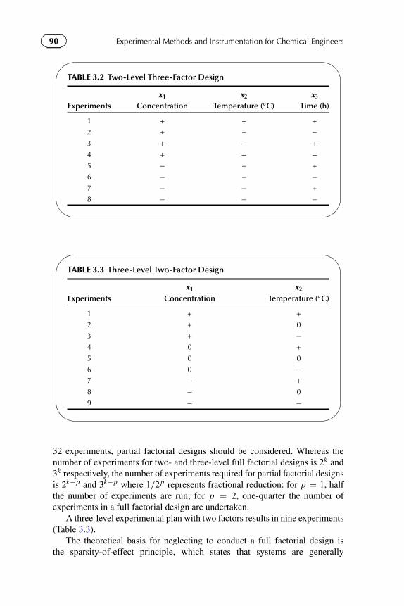
90 Experimental Methods and Instrumentation for Chemical Engineers�
�
�
�
TABLE 3.2 Two-Level Three-Factor Design
x1 x2 x3
Experiments Concentration Temperature (◦C) Time (h)
1 + + +
2 + + −3 + − +
4 + − −5 − + +
6 − + −7 − − +
8 − − −
�
�
�
�
TABLE 3.3 Three-Level Two-Factor Design
x1 x2
Experiments Concentration Temperature (◦C)
1 + +
2 + 0
3 + −4 0 +
5 0 0
6 0 −7 − +
8 − 0
9 − −
32 experiments, partial factorial designs should be considered. Whereas thenumber of experiments for two- and three-level full factorial designs is 2k and3k respectively, the number of experiments required for partial factorial designsis 2k−p and 3k−p where 1/2p represents fractional reduction: for p = 1, halfthe number of experiments are run; for p = 2, one-quarter the number ofexperiments in a full factorial design are undertaken.
A three-level experimental plan with two factors results in nine experiments(Table 3.3).
The theoretical basis for neglecting to conduct a full factorial design isthe sparsity-of-effect principle, which states that systems are generally
91Chapter | 3 Experimental Planning
dominated by main effects and low-order interactions (Montgomery, 2008).Thus, a subset of the full factorial is usually sufficient to characterize the entiresystem. The resolution of a fractional design is the difference k − p and is aproperty of a fractional design that indicates the ability to discriminate maineffects (x1,x2,x3, . . . ,xn) from low-order interactions (xi x j ). A resolution oftwo confounds main effects and is pointless. A resolution greater than five maydifferentiate higher-order effects but since most physical systems are bestdescribed by low-order effects, the effort to include them is unwarranted. Aresolution of three (k − p = 4 − 1 or k − p = 5 − 2, for example) and four aremost common. A resolution of three can estimate main effects but may be con-founded if two-factor interactions are significant. For example, in the followingequation, if the constant β12 is in the same order of magnitude or greater thanβ1/x2 or β2/x1 then a higher resolution is necessary:
y = β1x1 + β2x2 + β12x1x2. (3.23)
A resolution of four is adequate to identify main effects and two-factor inter-actions that are unconfounded with the main effects.
The assignments of the levels for each experiment are similar to those of afull factorial design except for columns greater than k − p. These columns areassigned based on a generator function. This function is typically a product ofthe columns less than or equal to k − p. Two restrictions apply to the columnsgenerated: their sequence must be different from any other column (or the matrixwill be confounded) and it must not be equal to any term that is a product oftwo or more factors already defined in the equation.
The Plackett-Burman design is a special case of partial factorial design thatapplies to experiments in which the number of runs (n) is a multiple of fourwith up to n − 1 factors. The Plackett-Burman design, as with other partialfactorial designs, is considered a screening design: it is adequate to identifythe main effects but higher-order effects and interactions are difficult to assess(Jeff Wu and Hamada, 2009). In this design, as shown in Table 3.4, each row isa cyclic permutation of the previous row (except for repeat runs or supplementruns needed to complete the square matrix).
Example 3.3. For the following equation, create a fractional factorial designwith a resolution of three and define three generator functions:
y = β1x1 + β2x2 + β2x3 + β4x4 + β12x1x2 + β23x2x3.
Solution 3.3. The design is shown below in Table E3.3. The generator functioncan be one of the following: the product x1x3 or x1x2x3, a constant value, or +or −. Although x1x2 and x2x3 would normally be possible generator functions,they are excluded because their products are part of the equation. If β0 were

92 Experimental Methods and Instrumentation for Chemical Engineers�
�
�
�
TABLE 3.4 Plackett-Burman Design for Eight Experiments and Six Factors
Experiments x1 x2 x3 x4 x5 x6
1 − + + − + −2 + + − + − −3 + − + − − +
4 − + − − + +
5 + − − + + −6 − − + + − +
7 + + + + + +
8 − − − − − −
�
�
�
�
TABLE E3.3 Partial Factorial Design
Experiments x1 x2 x3 x4 (1) x5 (2) x6 (3)x1x3 x1x2x3
1 + + + + + −2 + + − − − −3 + − + + − −4 + − − − + −5 − + + − − −6 − + − + + −7 − − + − + −8 − − − + − −
part of the function then a constant value for x4 would also be excluded to avoidconfounding.
3.4.4 Response Surface Designs
Response surface designs are the advanced stage of design. Screening designs—Plackett-Burman or fractional factorial, for example—identify the importantfactors; interaction designs—full factorial or fractional factorial with aresolution of five—substantiate the interactions between factors; finally,response surface designs allow for optimization, prediction, calibration, andeven process control adjustments. Examples of response surface designs includeBox-Behnken, Central Composite, and Face-Centered Cube. These topics areexamined in more advanced books on statistics.

93Chapter | 3 Experimental Planning
3.5 EXERCISES
3.1 (a) How many fitted parameters are there in the NIST equation for thespecific heat of methane?
C p,CH4 = −0.703029 + 108.4773T − 42.52157T 2 + 5.862788T 3
+ 0.678656T −2,
C p,CH4 = 85.81217 + 11.26467T − 2.114146T 2 + 0.138190T 3
− 26.42221T −2.
(b) How many parameters are there for the correlation proposed by VanWylen and Sonntag?
C p,CH4 = −672.87 − 439.74T −0.25 − 24.875T 0.75 − 323.88T −0.5.
3.2 The local television network wished to examine the accuracy of gas pumpsand collected 5 l samples from 10 different gas stations in the city. Theybrought gasoline samples to the university and were poured into a (2×2) lgraduated cylinder and a 1 l graduated cylinder and the temperature wasmeasured. After pouring the gasoline to the 2 l mark, the cylinder wasemptied then dried with paper towel before measuring again. Avoidingspillage was difficult because of the cramped space in the fume hood.The measured volume of gasoline, Vm , and the temperature data aresummarized in Table Q3.2. The reference temperature for the gasolinedispensed is 15 ◦C. To account for the thermal expansion of the gas, thefollowing equation is used to correct the measured volume to the volumeat the reference temperature, Vref:
Vref = Vm(Tm − 15) · 0.00124.
The NIST requires an accuracy of 0.3 vol%:
(a) Formulate a hypothesis statement for this experiment.(b) Are the gas stations compliant with the NIST regulation (i.e. does the
television station have something newsworthy to report)?(c) How could this experiment be improved?(d) Recommend five areas to improve the accuracy of this experiment.
�
�
�
�TABLE Q3.2 Volume of Gasoline Collected at 10 Stations
Vm (ml) 4978 5013 5000 5010 5010 5048 5000 5000 5020 4974
Tm (◦C) 21.8 21.9 21.9 22.4 22.5 22.4 22 21.8 21.8 21.4

94 Experimental Methods and Instrumentation for Chemical Engineers
(e) As a gas station operator and knowing that the uncertainty of thepump is 0.05%, how would you set the pump to avoid prosecutionbut to maximize profit?
3.3 Engineering students preferred Basmati rice over another well-knownbrand of long grain rice (Brand UB) and the reason cited for the prefer-ence was because the former was longer. The class was divided into 17groups and the grains were measured 10 times each. The measured lengthof the Basmati rice (in mm) was: 6.9, 7.0, 7.0, 6.9, 7.0, 6.8, 7.0, 6.5, 6.8,and 7.1. That of UB rice (also in mm) was: 6.5, 6.1, 6.6, 6.7, 6.2, 6.3, 6.9,6.3, 6.4, and 6.3:
(a) Formulate a null hypothesis and an alternative hypothesis statementto compare the length of the grains of rice for each type.
(b) Test the hypothesis and conclude if it should be accepted in favor ofthe alternative.
(c) As much as 10% of the Brand UB is broken in half. Should thesegrains be included in the study? If they were rejected, would thischange the conclusion?
3.4 (a) Propose a regression equation for a subset of the HadCRUT3 globaltemperature data given in Table Q3.4.
(b) Based on this equation, what will be the average global temperaturein 2020, 2050, and 2010?
(c) What is the likelihood that the global temperatures rise as high as thepredicted values from the regression equation? What are the possibleconsequences?
3.5 Let there be three factors whose variations are normalized from −1 to 1.The base case uses the combination (0,0,0). You can use eight additionalexperiments to build a regression model. Three models are considered:Bala Srinivasan
Y = β0 + β1 X1 + β2 X2 + β3 X3 + β12 X1 X2,
Y = β0 + β1 X1 + β2 X2 + β3 X3 + β11 X21,
Y = β0 + β1 X1 + β2 X2 + β3 X3 + β12 X1 X2 + β11 X21 .
(a) Propose eight new experiments using a full factorial design at twolevels.
(b) Propose eight new experiments using a fractional factorial design atthree levels (take X3 = X1 X2).
(c) What are the combinations of (a) and (b) with each of the modelsfor which there is a confounding factor when using only new exper-iments?
(d) What do you observe when using the base case in addition to newexperiments in the third model?

95Chapter | 3 Experimental Planning�
�
�
�
TABLE Q3.4 HadCRUT3 Global Temperature Data from 1960
Year �T (K) Year �T (K) Year �T (K)
1960 −0.1247 1977 0.0174 1994 0.1718
1961 −0.0236 1978 −0.0646 1995 0.2752
1962 −0.0219 1979 0.0492 1996 0.1371
1963 0.0015 1980 0.0762 1997 0.3519
1964 −0.2958 1981 0.1203 1998 0.5476
1965 −0.2161 1982 0.0100 1999 0.2971
1966 −0.1481 1983 0.1766 2000 0.2705
1967 −0.1495 1984 −0.0208 2001 0.4082
1968 −0.1590 1985 −0.0383 2002 0.4648
1969 −0.0109 1986 0.0297 2003 0.4753
1970 −0.0677 1987 0.1792 2004 0.4467
1971 −0.1902 1988 0.1799 2005 0.4822
1972 −0.0578 1989 0.1023 2006 0.4250
1973 0.0768 1990 0.2546 2007 0.4017
1974 −0.2148 1991 0.2126 2008 0.3252
1975 −0.1701 1992 0.0618 2009 0.4430
1976 −0.2550 1993 0.1058 2010 0.4758
3.6 Identify all combinations of four experiments to develop the followingmodel:
Y = β0 + β1 X1 + β3 X3 + β12 X1 X2.
See Table Q3.6.
3.7 The Young’s modulus (E) of an immiscible polymer depends on the fol-lowing: stretch during injection (ε), injection temperature (T), and theaddition of a fraction of fiberglass (F): B. Blais�
�
�
�
TABLE Q3.6 Example Model
Experiments Plan
1 −1 −1 −1
2 −1 −1 1
3 −1 1 −1
4 −1 1 1
5 1 −1 −1
6 1 −1 1
7 1 1 −1
8 1 1 1

96 Experimental Methods and Instrumentation for Chemical Engineers
(a) How many parameters are there for a linear model with no interac-tions?
(b) How many experiments are required to estimate the parameters? Out-line a full factorial design.
(c) During the first set of experiments, it is apparent that there is an inter-action between the stretch during injection and the injection temper-ature. Propose a new model to account for this interaction.
(d) How many experiments are required to determine the new parameterbased on a partial factorial experimental plan?
3.8 The fiber strength of electrospinning a new polymer depends on flow rate,solution concentration, electric potential, and temperature:
(a) Propose an experimental plan of eight experiments for a linear modelwith interactions. Assume the generator function for the fourth factoris X4 = X1 X2 X3.
(b) Discuss the problems of confounding for each of the following models:
Y = β0 + β1 X1 + β2 X2 + β3 X3 + β4 X4 + β123 X1 X2 X3,
Y = β0 + β1 X1 + β2 X2 + β3 X3 + β4 X4 + β124 X1 X2 X4,
Y = β0 + β1 X1 + β2 X2 + β3 X3 + β4 X4 + β12 X1 X2.
3.9 Typing speed varies based on the total number of words (Lt ) and thecomplexity of the vocabulary (Ct ) as shown in Table Q3.9 (TypeRacer®).Develop a linear model with interactions. Your equation must be of thetype:
P = β0 + β1Lt + β2Ct + β12 Lt Ct .�
�
�
�
TABLE Q3.9 Typing Speed
Typing Speed (wpm) Length of Text (words) Word Complexity (a.u.)
20 40 3
40 30 2.5
60 30 2.1
80 50 1.8
100 50 1.7
120 30 1
140 30 0.5
3.10 The distillation of ethanol and water solutions depends on concentrationand temperature (assuming near atmospheric pressure operation). Derivea cubic model with interactions up to third order. How many experimentsare needed? Would a fractional factorial design be sufficient to identifyall model parameters?
3.11 A paper bag manufacturer wishes to improve paper strength. The tearresistance is a function of the concentration of hardwood pulp from 5%

97Chapter | 3 Experimental Planning
to 20%. An experimental study designed to establish the relationshipbetween tear resistance and concentration includes four levels with sixrepeats at each level. The 24 specimens are tested randomly by a labora-tory dynamometer and the results are given in Table Q3.11. M.B. Moudio
(a) At a 99% confidence interval is the resistance independent of con-centration?
(b) If not, which concentration provides the greatest resistance?(c) Is this a multi-factorial problem?�
�
�
�
TABLE Q3.11 Hardwood Concentration
Hardwood Concentration (%) 1 2 3 4 5 6 Total Average
5 7 8 13 11 9 10 60 10.00
10 12 17 15 18 19 15 94 15.67
15 14 18 19 17 16 18 102 17.00
20 19 25 22 23 18 20 127 21.17
383 15.96
3.12 The Kraft process is the most common papermaking technique. Woodis chopped into pieces and cooked in caustic soda in a digester (reactor)operating at a constant temperature of 180 ◦C. The performance of thedigester (Y) depends on the type of wood:
Y = f (A,B,n),
where A,B, and n are factors related to the wood. T. Yasser
(a) Submit eight experiments using full factorial design at two levels.(b) Propose eight experiments using fractional factorial design at three
levels. Take n = AB.(c) We propose the following models:
Y = β0 + β1 A + β2 B + β3n + β12 AB + β13 An + β23 Bn
+ β11 A2 + β22 B2 + β33n2,
Y = β0 + β1 A + β2 B + β3n + β13 An + β23 Bn,
Y = β0 + β1 A + β2 B + β3n + β23 Bn.
(i) Write the regression matrix for each case.(ii) What are the models for which there is “confounding”? Justify
your answer using the regression matrix .(iii) If there is more than one model with no “confounding,” which do
you choose if we want to get better accuracy for the parametersof regression? Why?
(iv) Can we neglect the interaction between A and n (β13)? Why?

98 Experimental Methods and Instrumentation for Chemical Engineers
(d) We have 10 species of wood. For each case we have a value of A,B,and n (see Table Q3.12d). We propose the following model:
Y = β0 + β1 A + β2 B + β3n + β12 AB + β13 An + β23 Bn
+ β11 A2 + β22 B2 + β33n2.
�
�
�
�
TABLE Q3.12d Model Parameters for Wood
Species of Wood A B n
Western Hemlock (1) 96.8 4.84 0.41
Western Red Cedar (2) 84.1 4.68 0.35
Jack Pine (3) 94.3 5.88 0.35
Trembling Aspen (4) 85.5 1.37 0.76
Alpine Fir (5) 89.3 4.46 0.40
Balsam Fir (6) 87.5 4.32 0.40
Douglas Fir (7) 83.1 3.84 0.40
Hard Maple (8) 73.4 0.57 0.95
Red Alder (9) 66.1 0.41 0.95
Yellow Birch (10) 68.9 0.15 1.35
(i) Verify that the data allows us to find the regression coefficients.Justify your answer.
(ii) Find the values of regression coefficients.(iii) Propose two alternatives to reduce the variance of regression
parameters.
3.13 The relationship between the temperature and the pressure and the quan-tity of solvent to produce a pesticide follows a linear relationship withinteractions of the form: T.-V. Ton
Y = β0 + β1x1 + β2x2 + β12x1x2.
(a) Build a factorial design at two levels: x1 and x2 represent the quantityof solvent.
(b) Determine the matrix representing the problem.(c) Write the system to be solved.
3.14 Students in a biology class are experimenting on growing medicinalplants. They note that, at maturity, the length, x1, of the plant’s leavesranges from a minimum of 7 cm to a maximum of 15 cm. The height ofthe plant, x2, ranges from a minimum of 110 cm to a maximum of 135 cm.M.-M.L. Gilbert
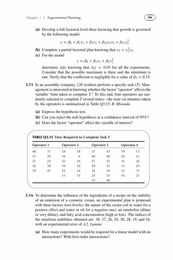
99Chapter | 3 Experimental Planning
(a) Develop a full factorial level three knowing that growth is governedby the following model:
y = β0 + β1x1 + β2x2 + β12x1x2 + β11x21 .
(b) Complete a partial factorial plan knowing that x3 = x31 x2.
(c) For the modely = β0 + β1x1 + β2x2
1
determine �β2 knowing that �y = 0.03 for all the experiments.Consider that the possible maximum is three and the minimum isone. Verify that the coefficient is negligible for a value of β2 = 0.15.
3.15 In an assembly company, 120 workers perform a specific task (T). Man-agement is interested in knowing whether the factor “operator” affects thevariable “time taken to complete T.” To this end, four operators are ran-domly selected to complete T several times—the time (in minutes) takenby the operators is summarized in Table Q3.15. R. Miranda
(a) Express the hypothesis test.(b) Can you reject the null hypothesis at a confidence interval of 95%?(c) Does the factor “operator” affect the variable of interest?�
�
�
�
TABLE Q3.15 Time Required to Complete Task T
Operator 1 Operator 2 Operator 3 Operator 4
48 37 24 18 37 43 19 13
31 29 16 6 40 40 26 21
31 24 22 24 51 35 31 26
36 38 10 30 49 33 13 24
39 41 25 24 36 39 12 12
11 15 24 55 16 21
35 40
3.16 To determine the influence of the ingredients of a recipe on the stabilityof an emulsion of a cosmetic cream, an experimental plan is proposedwith three factors (two levels): the nature of the cream (oil in water for apositive effect and water in oil for a negative one), an emulsifier (diluteor very dilute), and fatty acid concentration (high or low). The indices ofthe emulsion stabilities obtained are: 38, 37, 26, 24, 30, 28, 19, and 16,with an experimental error of ±2. Lamine
(a) How many experiments would be required for a linear model with nointeractions? With first-order interactions?

100 Experimental Methods and Instrumentation for Chemical Engineers
(b) Build an experimental plan for the model with first-order interactions.
3.17 The volume contraction, α, of aqueous glycerol solutions as a function ofweight fraction of glycerol is given in Table Q3.17.
(a) Determine the constant a for following expression that best fits thedata:
ρ = ax(1 − x2),
where x represents the glycerol mass fraction.(b) Calculate the coefficient of correlation, R2.�
�
�
�
TABLE Q3.17 Volume Contraction of Glycerol-Water Solutions at 20 ◦C
x 0 0.1 0.2 0.3 0.4 0.5 0.6 0.7 0.8 0.9 1
α (%) 0 0.225 0.485 0.705 0.948 1.08 1.101 1.013 0.814 0.503 0
Gerlach 1884.
3.18 The potential generated for a copper-constantan thermocouple versus tem-perature is given in Table Q3.18 (Holman, 2001):
(a) For each of the polynomial models given below, derive the coeffi-cients:
E = β0 + β1T ,
E = β0 + β1T + β2T ,
E = β0 + β1T + β2T + β3T .
(b) For each relationship, calculate the coefficient of correlation.
�
�
�
�
TABLE Q3.18 Copper-Constantan Thermocouple Potential VersusTemperature
◦C mV ◦C mV
−250 −6.18 100 4.279
−200 −5.603 150 6.704
−150 −4.648 200 9.288
−100 −3.379 250 12.013
−50 −1.819 300 14.862
0 0 350 17.819
50 2.036 400 20.872

101Chapter | 3 Experimental Planning
3.19 Derive a relationship between the emf and temperature differential of aType K thermocouple (see Table Q3.19).�
�
�
�
TABLE Q3.19 emf and Temperature Differential of Type K Thermocouple
�T (◦C) emf (mV) �T (◦C) emf (mV)
0 0 300 12.209
25 1 400 16.397
50 2.023 500 20.644
75 3.059 600 24.906
100 4.096 800 33.275
150 6.138 1000 41.276
200 8.139
3.20 A brigantine commutes between Tortuga Island and Cuba. The crossingtime depends on the load (in tonnes of rum), the phase of the moon,and the age of the crew (in years). The boatswain, using a full factorialexperimental design, noted the times in hours (Table E3.20): R. Taiebi
(a) Propose a linear model and a linear model with interactions.(b) Derive the constants for the linear model.(c) Is the age of the crew a significant factor?
�
�
�
�
TABLE E3.20 Crossing Time Between Cuba and Tortuga
Moon New Full New Full New Full New Full
Loading 20 20 100 100 20 20 100 100
Age 30 30 30 30 50 50 50 50
Time (h) 24 16 23 31 18 14 17 22
REFERENCES
Dunn, P., 1997. James Lind (1716–94) of Edinburgh and the treatment of scurvy. Archive ofDisease in Childhood Foetal Neonatal, United Kingdom: British Medical Journal PublishingGroup 76(1), 64–65. doi: http://dx.doi.org/10.1136/fn.76.1.F64. PMC 1720613. PMID 9059193.Retrieved 17.01.2009.
Fisher, R.A., 1918. The correlation between relatives on the supposition of mendelian inheritance.Philosophical Transactions of the Royal Society of Edinburgh 52, 399–433.
Gerlach, G.T., 1884. Chemistry Industry 7, 277–287.Jeff Wu C.F., Hamada, C.J., 2009. Experiments Planning, Analysis, and Optimization, 2nd ed.
Wiley.

102 Experimental Methods and Instrumentation for Chemical Engineers
Legg, T., 2012, April 4. Hadley Center Central England Temperature Dataset. Retrievedfrom Met Office Hadley Centre observations datasets: <http://www.metoffice.gov.uk/hadobs/hadcet/>.
Montgomery, D.C., 2008. Design and Analysis of Experiments, 7th ed. Wiley.Savitzky, A., Golay, M.J.E., 1964. Analytical Chemistry 36, 1627–1639.Thomke, S., Von Hippel, E., Franke, R., 1998. Modes of experimentation: an innovation process—
and competitive—variable. Research Policy 27, 315–332.White, J.W., 2004, June 11. VOL 304. Retrieved 2011, from sciencemag: <http://www.
climate.unibe.ch/stocker/papers/white04sci.pdf>.

Chapter 4
Pressure
4.1 OVERVIEW
In April 2010, gas and liquids from the Macondo oil well unexpectedly rosethrough the production casing (riser) to the surface and detonated on the DeepHorizon ultra-deepwater offshore drilling rig. Two days later, the rig sank andgas and oil continued to gush from the well on the sea floor 1600 m below thesurface for several months causing the worst environmental disaster in Americanhistory. The blow out was caused by a combination of mechanical failure, poorjudgment, and operational design, but correctly interpreting the pressure testcould have averted this catastrophe. During the preparation for the temporaryabandonment, BP replaced drilling mud (density of 1740 kg m−3) with seawater (density of 1030 kg m−3) (Graham et al, 2011). The hydrostatic head ofthe sea water (ρgh) was presumably insufficient to avoid hydrocarbons fromentering the well. Consequently, gas and liquids rose up through the well fromseveral thousand meters below the surface of the floor bed. When it reached theplatform, the methane gas entered the ventilation system and ignited, resultingin a fireball that was visible for over 35 mi. Oil and natural gas leaked throughthe riser for three months and the rate peaked at over 62 000 bbl d−1 and someestimate that it could have been more than 80 000 bbl d−1.
Pressure measurement is a critical factor not only in the oil and gas industrybut also for the operation of process equipment including reactors, distillationcolumns, pipelines, and for the measurement of flow rate. It is a scalar quantityand equals the perpendicular force exerted on a surface with the units of forceper surface area:
P = F
A= N
m2 = Pa. (4.1)
Experimental Methods and Instrumentation for Chemical Engineers. http://dx.doi.org/10.1016/B978-0-444-53804-8.00004-6© 2013 Elsevier B.V. All rights reserved. 103

104 Experimental Methods and Instrumentation for Chemical Engineers
Pressure together with temperature, flow rate, and concentration are theessential macroscopic properties required to operate chemical processes.Various units are frequently used to report pressure and some common unitsand their conversions are reported in Table 4.2.
Atmospheric pressure is a result of the hydrostatic head of air ρgh andequals 101 325 Pa (at sea level and a clear day). However, the Aristotelianview was that air was weightless. It wasn’t until the Renaissance that Toricellichallenged this postulate. To avoid being accused of witchcraft and sorcery, heworked secretly and invented the mercury (“quicksilver”) barometer to conductexperiments in an instrument measuring only 80 cm in height compared to awater column of over 10 m that was commonly used at the time. Pascal wasthe first to demonstrate that pressure changed with elevation by measuring theheight of mercury in a barometer at the base of the Puy de Dome and along itsheight to the summit at 1464 m.
Together with columns of liquids, other forms of pressure common tothe process industry include the pressure of gases in vessels, vapor pressure,dynamic pressure, and pressure drop across pipes, flow meters and throughporous materials. At constant pressure and a fixed mass, Boyle’s law states thatfor an ideal gas, the volume and absolute pressure are inversely proportional:
PV = c (4.2)
orP1V1 = P2V2. (4.3)
As the pressure of an ideal gas increases, its volume decreasesproportionately. Charles’ law describes the relationship between the volumeand temperature of an ideal gas at constant pressure:
V1
T1= V2
T2. (4.4)
The volume increases proportionally with temperature. Amontons’ lawrelates pressure and temperature and can be derived from Boyle’s and Charles’laws:
P1
T1= P2
T2. (4.5)
The ideal gas law relates the product of pressure and volume to temperatureand the number of moles:
PV = n RT , (4.6)
where n is the number of moles and R is the ideal gas constant (which is equalto 8.314 J mol−1 K−1).
This relation may be derived from the kinetic theory of gases. Pressureis a result of momentum exchange between molecules and a confining wall
105Chapter | 4 Pressure
(in the example of a vessel). This exchange varies with the frequency ofcollisions together with the speed of the molecules and is given by
P = 1
3nmv2
rms, (4.7)
where n is the number of molecules per unit volume (N/V ), m is the molecularweight (mass) of the gas molecule, and vrms is the root mean square molecularvelocity.
The root mean square velocity is related to absolute temperature andmolecular mass by the following relation:
1
2mv2
rms = 3
2kT , (4.8)
where k is Boltzmann’s constant (1.3806 × 10⁻²³ J mol−1 K−1). Thus:
P = 1
3nmv2
rms · 3kT = 1
VNkT = 1
Vn RT . (4.9)
The ideal gas constant, R, is the product of Boltzmann’s constant andAvogadro’s number—the number of molecules in one mole (6.022 × 10²³).
Example 4.1. What is the temperature and the root mean square velocity ofone mole of helium in a one liter flask maintained at
(a) 1 atm.(b) 10 atm.(c) At what pressure will the temperature in the flask reach 0 ◦C.
Solution 4.1a. First the temperature is calculated based on the ideal gas law.The value of the temperature is then used in the equation relating kinetic energyand temperature:
PV = n RT ,
so
T = PV
nR.
We know that V = 1 l, n = 1 mol, and R = 8.314 J mol−1 K−1, so:
T = 1 atm · 101 325 Pa atm−1 · 1 l · 0.001 m3 l−1
1 mol · 8.314 J mol−1K−1 = 12.2 K.
Finally:1
2mv2
rms = 3
2kT ,
106 Experimental Methods and Instrumentation for Chemical Engineers
so
m = 4 g mol−10.001 kg g−1
6.023 × 10²³ molecule mol−1 = 6.641 × 10⁻²⁷ kg molecule−1
and
vrms =√
3
mkT
=√
31.3806 × 10⁻²³ J molecule−1 K−112.2 K
6.641 × 10⁻²⁷ kg molecule−1
=√
76 088 m2 s2 = 276 m s−1.
Solution 4.1b. We can apply Charles’ law to calculate the temperature at thehigher pressure:
P1V1
T1= P2V2
T2,
T2 = T1P2V2
P1V1= 12.2 K
10 atm
1 atm= 122 K,
vrms,122 = vrms,12.2
√122
12.2= 872 m s−1.
Solution 4.1c. In this example, pay attention to the units: there are 4 g of Hein one liter, which translates to 4 kg of He in 1 m3. SI units require kg and m3
but all the values are given in cgs:
vrms,273 = vrms,12.2
√273
12.2= 1300 m s−1,
P = 1
3nmv2
rms,273
= 1
36.023 × 1026molecule m−3 · 6.641 × 10−27 kg molecule−1
·(1300 m s−1)2
= 2253 kPa = 22.2 atm.
The ideal gas law characterizes the relationship between pressure,temperature, and volume for gases. Both the Clausius-Clapeyron and Antoineequations characterize the vapor-liquid equilibrium of pure components andmixtures. At atmospheric pressure and ambient temperature, water is a liquidbut an equilibrium exists with its vapor phase concentration—its vapor pressure.The vapor pressure is a function of temperature. The formula for the Clausius-Clapeyron equation is:
ln P◦ = −�HvRT
+ BCC , (4.10)
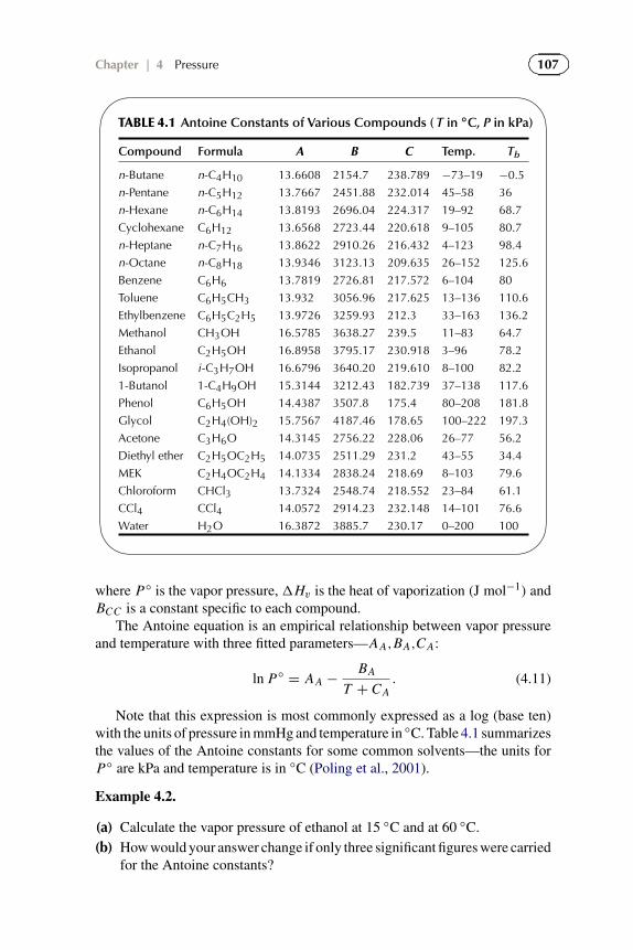
107Chapter | 4 Pressure�
�
�
�
TABLE 4.1 Antoine Constants of Various Compounds ( T in ◦C, P in kPa)
Compound Formula A B C Temp. Tb
n-Butane n-C4H10 13.6608 2154.7 238.789 −73–19 −0.5
n-Pentane n-C5H12 13.7667 2451.88 232.014 45–58 36
n-Hexane n-C6H14 13.8193 2696.04 224.317 19–92 68.7
Cyclohexane C6H12 13.6568 2723.44 220.618 9–105 80.7
n-Heptane n-C7H16 13.8622 2910.26 216.432 4–123 98.4
n-Octane n-C8H18 13.9346 3123.13 209.635 26–152 125.6
Benzene C6H6 13.7819 2726.81 217.572 6–104 80
Toluene C6H5CH3 13.932 3056.96 217.625 13–136 110.6
Ethylbenzene C6H5C2H5 13.9726 3259.93 212.3 33–163 136.2
Methanol CH3OH 16.5785 3638.27 239.5 11–83 64.7
Ethanol C2H5OH 16.8958 3795.17 230.918 3–96 78.2
Isopropanol i-C3H7OH 16.6796 3640.20 219.610 8–100 82.2
1-Butanol 1-C4H9OH 15.3144 3212.43 182.739 37–138 117.6
Phenol C6H5OH 14.4387 3507.8 175.4 80–208 181.8
Glycol C2H4(OH)2 15.7567 4187.46 178.65 100–222 197.3
Acetone C3H6O 14.3145 2756.22 228.06 26–77 56.2
Diethyl ether C2H5OC2H5 14.0735 2511.29 231.2 43–55 34.4
MEK C2H4OC2H4 14.1334 2838.24 218.69 8–103 79.6
Chloroform CHCl3 13.7324 2548.74 218.552 23–84 61.1
CCl4 CCl4 14.0572 2914.23 232.148 14–101 76.6
Water H2O 16.3872 3885.7 230.17 0–200 100
where P◦ is the vapor pressure,�Hv is the heat of vaporization (J mol−1) andBCC is a constant specific to each compound.
The Antoine equation is an empirical relationship between vapor pressureand temperature with three fitted parameters—AA,BA,CA:
ln P◦ = AA − BA
T + CA. (4.11)
Note that this expression is most commonly expressed as a log (base ten)with the units of pressure in mmHg and temperature in ◦C. Table 4.1 summarizesthe values of the Antoine constants for some common solvents—the units forP◦ are kPa and temperature is in ◦C (Poling et al., 2001).
Example 4.2.
(a) Calculate the vapor pressure of ethanol at 15 ◦C and at 60 ◦C.(b) How would your answer change if only three significant figures were carried
for the Antoine constants?
108 Experimental Methods and Instrumentation for Chemical Engineers
Solution 4.2a. The Antoine constants for ethanol are AA = 16.8958,BA = 3795.17,CA = 230.918:
ln P◦ = AA − BA
T + CA= 16.8958 − 3795.17
15 + 230.918,
P◦15 = e1.46314 = 4.3 kPa,
P◦60 = e3.85030 = 47 kPa.
Solution 4.2b. This is a clear example where too many significant figuresare carried with respect to the constants in the correlation (with respect to thenumber of significant figures reported for temperature)
ln P◦ = AA − BA
T + CA= 16.9 − 3800
15 + 231,
P◦15 = e1.453 = 4.3 kPa,
P◦60 = e3.841 = 47 kPa.
4.2 UNITS OF PRESSURE
The SI unit for pressure is the Pa but for many calculations the kPa is adopted toreduce the number of digits in calculations. Until 1999, 1 atm had been acceptedas the standard reference pressure in chemistry, in the oil and gas industry, forequipment specifications, etc. However, the IUPAC (International Union of Pureand Applied Chemistry) redefined standard pressure to equal 100 kPa and thisis designated as 1 bar. In the Imperial system of units, the measure of pressureis psi and, as shown in Table 4.2, 14.696 psi equals 1 atm; 14.504 psi equals1 bar. For assessing vacuum, standard units are Torr, mmHg, and µm. Thereare 760 mmHg in 1 atm and 1 Torr equals 1 mmHg; 1 µm is 0.001 Torr. Whilemercury is commonly used in barometers to measure atmospheric pressure,water is used in manometers; its lower density offers a greater precision (for thesame pressure drop). In the Imperial system, the units of differential pressureare often quoted in are inH2O (1 inH2O = 25.4 mmH2O).
4.3 TYPES OF PRESSURE
Pressure in the chemical industry covers a range of at least 12 orders ofmagnitude: natural gas pipelines operate at 200 bar; in three-phase gas-liquid-solid hydrogenation reactors, pressures can exceed 150 bar to achieve a highconcentration of hydrogen in the liquid phase; many catalytic processes operatebetween 1 bar and 10 bar; vacuum distillation towers in oil refineries maybe as large as 15 m in diameter and operate at 25 mmHg; freeze drying iscommon for preparing vaccines and antibiotics and to store blood and plasma

109Chapter | 4 Pressure�
�
�
�
TABLE 4.2 Common Pressure Units and Their Conversions
kPa mmH2O mmHg psi inH2O inHg
kPa – 101.975 7.5006 0.14504 4.0147 0.2953
mmH2O 0.009806 – 0.073556 0.001422 0.03937 0.002896
mmHg 0.133322 13.595 – 0.019337 0.53524 0.03937
psi 6.894757 703.0875 51.7151 – 27.6787 2.03601
inH2O 0.249082 25.4 1.86833 0.036129 – 0.07356
inHg 3.3864 345.313 25.4 0.49116 13.595 –
FIGURE 4.1 Types of Pressure
at pressures around 10−4 Torr; pressures below 10−6 Torr are required foranalytical equipment such as electron microscopes and mass spectrometers.The lowest recorded pressure (up until 1991) was by a Japanese team whoreached 7 × 10⁻¹³ mbar. Standard definitions of pressure are illustrated inFigure 4.1.
4.3.1 Atmospheric Pressure
Atmospheric pressure at sea level is 101 325 Pa and this is defined as 1 atm.The pressure reported by meteorological stations is usually the mean sea levelpressure (MLSP): this is the pressure that would be calculated if the station wereat sea level. Thus, the MLSP reported by the meteorological service at Denver,Colorado (at 1665 m) is much higher than the actual reading of a barometerlocated in the city.

110 Experimental Methods and Instrumentation for Chemical Engineers
4.3.2 Gauge Pressure
Pressure gauges often read zero at atmospheric conditions, whereas in realitythey should read one atmosphere (or the barometric pressure); therefore, whena pressure indicator reaches a value of 2 atm, for example, the true pressureis in fact 3 atm. The value of 2 atm is referred to as the gauge pressure.To distinguish between gauge and absolute pressure, the letter “g” or“a” is added to the end of the unit: 4.5 barg = 5.5 bara = 65 psig = 80 psia.Remember that there is a relative difference between bar and atm of1.3%, which is negligible when carrying two significant figures but mustbe accounted for when carrying more significant figures or calculatingdifferential pressure or very high pressures. Thus, if the gauge is quoted inbar, 4.500 barg = 5.513 bara = 5.4410 atma.
4.3.3 Differential Pressure
Ideally differential pressure is measured with a single instrument: the upstreampressure in a flowing fluid is at the higher pressure and the pressure tapdownstream is at the lower pressure. The precision of differential pressure gaugeis significantly greater than subtracting the difference between two pressuregauges.
Example 4.3. Compare the precision of a differential pressure gauge versusthat of subtracting the measurements of two pressure gauges in a systemoperating at 3 barg. The full-scale pressure on the gauges is 5 barg whereas it is100 mbar for the differential pressure gauge and the precision of the instrumentsis ±0.01%.
Solution 4.3. Manufacturers may quote the precision either as an absolutevalue or as a percentage. When it is quoted as a percentage, the reference pointis the full-scale measurement. In this case, the precision of the differentialpressure gauge is 0.01 bar, whereas it is 0.05 bar for the two pressure gauges.The uncertainty of the differential pressure measured by the two gaugesindependently is calculated according to:
� f =√√√√ n∑
i=1
(ai�i )2. (4.12)
So,
��P =√�2
P1+�2
P2= �P1
√2 = 0.05 bar · √
2 = 0.07 bar.
4.3.4 Vacuum Pressure
Vacuum is measured relative to atmospheric pressure. Outer space is close toabsolute vacuum: the pressure is close to 0 bar but the vacuum is approximately

111Chapter | 4 Pressure
1.01325 bar. Various analytical instruments operate below 10−6 Torr and someprocesses in the pharmaceutical industry may operate at these low pressures.Chemical processes—distillation columns, for example—may operate at25 Torr.
Example 4.4. A process is designed to operate at a vacuum of 0.60 bar. Whatis its operating pressure in Torr?
Solution 4.4. Taking atmospheric pressure equal to 1.01 bar, the pressure ofthe process equals:
P = (1.01 bar − 0.60 bar) · 1 atm
1.0133 bar· 760 Torr
1 atm= 308 Torr ∼ 310 Torr.
The vacuum pressure is seldom used for instrumentation equipment—theabsolute pressure is quoted.
4.3.5 Static vs. Dynamic Pressure
Pressure manifests itself under both static and dynamic conditions—the bottomof a lake or the sea is an example of static conditions while both wind blowing orliquid flowing through a pipe are examples of dynamic pressure. The pressure(Pa) at the bottom of a tank or reservoir is equal to the hydrostatic head of theliquid:
P = ρgh, (4.13)
where ρ is the fluid density (kg m−3), g is the gravitational constant (m2/s)and h is the height of liquid in the vessel (m).
Note that the pressure exerted is independent of the geometry: for each of thevessels shown in Figure 4.2 the pressure at the bottom of the column of liquidis equal. The general integral to calculate pressure is expressed as a function ofvertical distance, z (m):
∫ 2
1d P =
∫ 2
1ρ(z)g dz. (4.14)
h
FIGURE 4.2 Equivalence of Static Head

112 Experimental Methods and Instrumentation for Chemical Engineers
In many cases, the fluid density is constant along the column length. Thusthe integral becomes:
P2 − P1 = ρg(z2 − z1),
�P = ρg�z.
For the case where the vessel is open to atmosphere, P1 = 0 atmg and thusthe gauge pressure is simply equal to the hydrostatic head.
For multi-phase fluid flow (gas-solid, gas-liquid, gas-solid-liquid, etc.)through vertical pipes and vessels, the density often decreases with height.As a first approximation, the pressure drop is assumed to be due entirely to thehydrostatic head of the fluid and the solids (frictional and inertial contributionsto the pressure drop are assumed to be negligible—which can introduce an errorof up to 10%). The suspension density for a gas-solids system is:
ρ = ρgε + ρp(1 − ε),
where ρg is the gas density (kg m−3), ρp is the particle density (kg m−3), andε is the void fraction.
In the case of air transporting a catalyst at near-atmospheric conditions, thisequation may be simplified by neglecting the contribution of the gas density.The transport of petroleum from oil reservoirs is more complicated: (a) gasdensity in deep wells may be significant; (b) the gas density increases along thelength of the pipe; and (c) because of the higher gas velocity the velocity of theliquid phase also increases and thus the void fraction also increases.
Dynamic pressure is measured normal to the direction of a flowing fluid andincreases with both an increase in velocity and fluid density:
P = 1
2ρu2
f . (4.15)
Example 4.5. When you extend your arm outside the window of an automobiletraveling at a high velocity, the air pushes the arm backwards—it experiencesdynamic pressure. At what velocity would a car have to travel for a handextended out of a window to feel the same dynamic pressure as what it wouldfeel in water?
Solution 4.5. The first assumption is that the pressure is atmospheric and thetemperature is 25 ◦C (and the relative humidity is zero). We calculate the densityof the air from the composition of the major constituents—nitrogen (78.1%),oxygen (20.%), and argon (0.9%).
Mm ≈ yO2 Mm,O2 + yN2 Mm,N2 + yAr Mm,Ar
= 0.210 · 32.0 + 0.781 · 28.0 + 0.009 · 40.0 = 28.948 = 28.9,
ρ = P
RT= 1.01325 atm
0.082059 m3 atm kmol−1 K−1 298.15 K= 0.041415 kmol m−3
ρ = Mm ρ = 28.9 kg kmol−10.0414 kmol m−3 = 1.20 kg m−3.

113Chapter | 4 Pressure
The density of water is 1000 kg m−3 and to achieve the same dynamic velocityin air as water, the air velocity will equal the product of the water velocity andthe square root of the ratio of the densities:
PH2O = Pair = 1
2ρu2
f ,
uair = uH2O
√ρH2O
ρair= uH2O
√1000
1.20= 28.9 uH2O ≈ 30 uH2O.
The sum of the static and dynamic pressures is termed the stagnation pressureor total pressure.
4.3.6 Barometric Pressure
Barometric pressure changes throughout the day and may even change severalpercent in an hour: skies are clear at high pressure whereas low pressures areaccompanied by clouds and often precipitation. Figure 4.3 illustrates the changein barometric pressure in Montreal during an entire year. The maximum pressurewas 103.1 kPa, while the minimum pressure was 96.5 kPa. The maximumchange in pressure from one day to the next during the year was 4.5 kPa.The lowest barometric pressure ever recorded at sea level was during a typhoonin the Pacific Ocean at 87.0 kPa in 1979.
Together with barometric pressure, two other factors that are generallyneglected in experimental data analysis are the effects of elevation and gravity.The gravitational “constant,” g, varies with latitude. Its value is greatest at thepoles at approximately 9.83 m2 s−1, as shown in Figure 4.4, and it is lowerby 0.5% at the equator at 9.78 m2 s−1. The following equation adequatelyapproximates the variation of gravity with latitude for most engineeringcalculations:
g = 9.780372(1 + 0.0053024 sin2 θ − 0.0000058 sin2 (2θ)). (4.16)
FIGURE 4.3 Variation of Atmospheric Pressure During 2006 in Montreal (Environment Canada,2011)

114 Experimental Methods and Instrumentation for Chemical Engineers
FIGURE 4.4 Relationship Between the Gravitational Constant, g, and Latitude
Elevation has a more appreciable impact on barometric pressure comparedto the gravitational constant as shown in Table 4.3. Pascal proved that barometricpressure was caused by the weight of air and that as the elevation increases thepressure decreases.
d P
d Z= ρg.
For an ideal gas, the molar density is a function of temperature, pressure,and gas composition:
ρ = Mm P
RT= P
RT.
The molar mass, Mm , of air is 28.95 kg kmol−1 and thus the value of R is287 J kg−1 K−1. Substituting this relation into the differential equation relatingpressure and elevation gives:
d P
d Z= P
RTg.
This equation, when integrated, approximates the pressure poorly because itignores the change in temperature with height: Figure 4.5 illustrates the variationof atmospheric temperature with elevation. The temperature decreases linearlywith elevation in the troposphere and mesosphere but it increases with elevationin the stratosphere and thermosphere:
T = To + mθ Z .

115Chapter | 4 Pressure�
�
�
�
TABLE 4.3 Atmospheric Pressure Variation with Elevation
z (m) P (Pa) z (m) P (Pa)
0 101 325 12 192 18 822
457 95 950 15 240 11 665
1067 89 150 21 336 4488
1524 84 309 30 480 1114
1676 82 745 40 000 270
1981 79 685 42 672 201
2591 73 843 45 000 130
3048 69 693 50 000 70
6096 46 599 58 000 30
9144 30 148 63 000 13
10 668 23 988 77 000 1.3
FIGURE 4.5 Atmospheric Temperature Variation with Elevation
To accurately calculate the pressure variation, the temperature variation withelevation must necessarily be included:
d P
d Z= P
R(To + mθ Z)g.
Isolating pressure and elevation gives:∫ P
Po
d P
P=∫ Z
0
g
R(To + mθ Z)d Z .

116 Experimental Methods and Instrumentation for Chemical Engineers
The integral becomes:
lnP
Po= − g
mθ Rln (To + mθ Z)− ln To.
This expression may be rearranged to give the following:
P = Po
(1 + mθ Z
To
)−mθ R/g
.
In the troposphere, the temperature drops by about 6.5 ◦C for every1000 m (mθ = −0.0065 K m−1) while it increases by about 1.8 ◦C forevery 1000 m in the stratosphere (mθ = 0.0018 K m−1).
So, from 0 km to 11.5 km, the equation relating pressure to elevation is:
P = Pbaro(1 − 0.0000226Z)5.25. (4.17)
The value of Pbaro equals the barometric pressure (which equals 1 atm onsunny days!). From 20 km to 50 km, the equation relating pressure to elevationis:
P = 0.0628
(1 + 0.0018
216(Z − 20000)
)−19.0
. (4.18)
The pressure at any elevation may be derived analytically by consideringthe temperature variation in each zone. At 70 km, for example, the temperatureis constant in part of the stratosphere and mesosphere and varies with elevationin both these zones as well as the troposphere. The resulting expression iscumbersome and remains an approximation if the change in the gravitationalconstant with elevation is ignored:
gZ = g
(re
re + Z
)2
, (4.19)
where re is the radius of the earth (6.371 × 10⁶ m). Rather than calculatingthe exact pressure variation analytically, an approximate model may be derivedthrough a regression analysis—curve fitting. Parameters in models representphysical phenomena, whereas in curve fitting models they generally have nophysical significance. The advantage of curve fitting is that simple expressionsmay be derived that adequately approximate the data.
Figure 4.6 demonstrates the pressure as a function of elevation and inFigure 4.7 the data is replotted in terms of the log of pressure. (Note thatindependent variables are usually reserved for the vertical—y-axis. In this case,the dependent variable, P, is shown on the x-axis and elevation is on the y-axis.This designation was adopted to represent the physical phenomena—elevationis in the vertical direction.) While it would be difficult to read the data at

117Chapter | 4 Pressure
FIGURE 4.6 Atmospheric Pressure Variation with Elevation
FIGURE 4.7 Atmospheric Pressure (log) Variation with Elevation
elevations above 25 km, the data is more obvious in Figure 4.7—the log ofpressure appears to drop linearly with elevation.
The fit between the experimental data and the expression for the elevationin the troposphere is incredibly good with an R2 = 0.9999996. (The agreementbetween data and model is so good that it is unlikely that the data is experimentalbut rather derived from the model.) The CRC reports an expression for theelevation as a function of pressure:
P = 100
(44331.514 − Z
11880.516
)1/0.1902632
. (4.20)
This expression has several fundamental deficiencies: in the first place,there are too many significant figures. Considering that atmospheric pressuremay vary by as much as 4% in a single day, it is unreasonable to carry eightsignificant figures for any fitted parameter (ever). Also, there are too many

118 Experimental Methods and Instrumentation for Chemical Engineers
fitted parameters: the coefficients 100 and 11 880.516 are 100% correlated. Infact, this expression is almost exactly equivalent to the model derived for thetroposphere!
Regardless of the formulation, Figure 4.7 shows that the expression deviatessignificantly from the data at elevations above 12 000 m, which is expected sincethe model was derived for the troposphere. Recognizing that log P decreaseslinearly with elevations up to 70 km, we propose a two-parameter model (wherethe units of Z are km):
P = Po exp(−0.114Z1.07
). (4.21)
At sea level (Z = 0), the pressure equals 1.01325 kPa and it increasesexponentially with Z to the power 1.07. Based on Figure 4.7, we could concludethat this relationship fits the data very well up to 80 km. Figure 4.8 showsa deviation of no more than 10 mbar up until 20 km and then the absolutedeviation approaches a very small number. The deviation between the predictedand experimental pressure of the physical model reaches 2 mbar up until thestratopause and then reaches a maximum of 12 mbar before dropping again.The percent deviation in the troposphere is superior for the physical model butthe curve fit characterizes the entire data set very well. The error is as high as50% in the mesosphere but the absolute difference between data and curve fitis only 0.006 mbar at 77 km.
As a practical example of the significance of elevation in chemical processes,consider the steam extraction of essential oils. Low temperatures are preferredto extract oil from plants because of their susceptibility to degradation. Thus,an alternative to vacuum extraction would be to operate at higher elevation.
ΔP, mbar-20 0 20 40 60
Elev
atio
n, k
m
0
20
40
60
80
Δ Pmodel, %
-20 0 20 40 60
FIGURE 4.8 Model Comparisons versus Elevation (mbar and %)

119Chapter | 4 Pressure
Example 4.6. Using the Clausius-Clapeyron equation, calculate at whatelevation water boils at 90 ◦C. The heat of vaporization of water is40.66 kJ mol−1.
Solution 4.6. Since the boiling point of water at atmospheric pressure isknown, the Clausius-Clapeyron equation can be rearranged to replace theconstant BCC :
lnP
◦2
P◦1
= −�HvR
(1
T2− 1
T1
).
Therefore, the pressure at which water boils at 90 ◦C becomes:
P2◦ = P1
◦ exp
(−�Hv
R
(1
T2− 1
T1
))
= 1 · exp
(− 40 660 J mol−1
8.314 J mol−1 K−1
(1
363 K− 1
373 K
))= 0.70 atm.
Expressing the elevation as a function of pressure gives:
Z = 1
0.0000226
((P1
P2
)0.19
− 1
)= 1
0.0000226
((1
0.7
)0.19
− 1
)=3100 m.
4.4 PRESSURE MEASUREMENT INSTRUMENTATION
As with most physical properties such as pressure, temperature, humidity,viscosity, etc. analytical instruments measure something other than the propertyof interest. A signal is recorded—current, voltage, change in height, ordeflection—and is then compared to a standard. A basic limitation of allmeasurements is the necessity of a standard or reference point. In the caseof pressure, a good reference point would be absolute vacuum, which is, inpractice, impossible to achieve and thus a non-zero quantity is adopted as astandard. The standard for most industrial applications is atmospheric pressure,which is itself a poor standard as we have already seen that atmospheric pressurechanges by as much as 6% throughout the year.
Several terms for pressure measuring devices are used interchangeablyincluding transmitters, transducers, gauges, sensors, and manometers. Moreprecisely, a gauge is a self-contained device that converts a force fromthe process to a mechanical motion of needle or other type of pointer.A manometer is a term reserved for an instrument that measures the hydrostatichead of a liquid and generally operates near atmospheric pressure. A transduceror transmitter combines the sensor with a power supply and a converter—generally mechanical-to-electrical or mechanical-to-pneumatic. The sensor

120 Experimental Methods and Instrumentation for Chemical Engineers
refers to the element that is sensitive to changes in pressure and may eitherbe a mechanical deviation or a change in electrical current.
In general, pressure measurement devices may be classified as eitherelectrical or mechanical. The first sensors were mechanical and relied onflexible elements. Because of the limitations of mechanical motion devices,wire strain gauges were then adapted to measure pressure. Capacitancetransducers were developed for vacuum applications. A potentiometric deviceis attached to a bellows element and converts a mechanical deflection into anelectrical signal using a Wheatstone bridge circuit. Resonant wire transducersmeasure a wide range of pressures from vacuum at 10 Torr up to 42 MPa.They consist of a wire attached to a sensing diaphragm at one end and fixed atthe other. The wire vibrates at its resonant frequency due to an oscillator circuit.Changes in pressure result in a change in the resonant frequency of the wire.
Factors influencing the choice of an instrument depend primarily on thepressure of the application and whether the gauge is required for control orsimply as an indicator. For control, electronic transmitters are preferred whereasmechanical devices are suitable as indicators. Mechanical indicators are easyto read and interpret but may be difficult to install in tight areas or mayrequire extensive tubing. Electronic transmitters may be easier to install in tightareas or remote connections but require a power supply and wire, as well asadditional displays. The dynamic response of electrical instruments is superiorto mechanical indicators since the data can be recorded at high frequency.
4.4.1 Barometer
The barometer is perhaps the simplest pressure gauge and it is still commonlyfound in laboratories to assess barometric pressure. It is one of the fewinstruments that measures absolute pressure. Before Toricelli, water columnsof 10.3 m were necessary to study pressure. Toricelli invented the mercurybarometer with a density 13.6 times that of water thus the column height isnever much more than 0.9 m. The barometer is composed of a tube, a pool ofmercury as well as a scale to measure distance and a vernier used to assess theexact position on the scale to a precision of 0.1 mm.
The tube filled with mercury is immersed in the reservoir of mercury.The height of mercury in the column increases as the pressure increases (theatmospheric pressure exerts itself on the pool of mercury forcing the liquid levelto rise). At 1 atm of pressure, the height of the Hg column should equal 760 mmat sea level. At 1 bar pressure, the height of the column is 750.06 mm.
4.4.2 U-Tube Manometer
In undergraduate laboratories, the most common differential pressuremeasurement device is the U-tube manometer. As shown in Figure 4.9, the

121Chapter | 4 Pressure
FIGURE 4.9 U-Tube Manometer
principal component is a tube in the shape of a U half filled with a fluid with adensity, ρm . In the figure, a restriction in the pipe causes a pressure drop suchthat the pressure at point 1 is higher than at point 2. The difference in height,�z, reflects the magnitude of the pressure differential. When the pressure atpoint 1 equals that at point 2 (when there is no flow), the height of the fluid ineach leg of the tube is equal. As the flow increases, the height z1 will begin todrop and z2 will rise correspondingly (as long as the diameters on both sidesof the tube are equal). The change in height,�z, is calculated based on a forcebalance: the pressure at the top of the meniscus in leg 1 is equal to the sum ofthe pressure and the hydrostatic head of the fluid. In leg 2, the pressure at thesame height equals the sum of the hydrostatic head of the fluid (z2), the headof the fluid in the manometer (�z), and the pressure at point 2:
P1 + ρflgz1 = P2 + ρflgz2 + ρm g�z, (4.22)
where ρfl is the fluid density in the pipe (kg m−3) and ρm is the fluid density inthe manometer (kg m−3).
The pressure differential is written as:
P1 − P2 = ρflgz2 − ρflgz1 + ρm g�z,
�P = (ρm − ρfl)g�z.
Under most conditions when measuring the pressure drop of a gas, its densitymay be ignored, as ρm � ρfl. When the second leg is open to atmosphere, themanometer reading represents the gauge pressure—the absolute pressure willequal the pressure differential plus the barometric pressure.

122 Experimental Methods and Instrumentation for Chemical Engineers
FIGURE 4.10 Inclined U-Tube Manometer
Common fluids used in the manometer are mercury, water, and oil.Maximum pressure differentials achievable are higher with mercury but theprecision is much less than one-tenth compared to water. Certain types of oilshave a density of around 800 kg m−3 and thus the measured �P has a 25%higher sensitivity versus water. In order to increase the sensitivity, the secondleg may be inclined, as shown in Figure 4.10.
Example 4.7. The low pressure leg of a U-tube manometer is exposed toatmospheric pressure and is inclined at an angle of 30◦ from the horizontal. Thetube diameter is 0.005 m and water is used as the measuring fluid. The resolutionof the ruler to measure the displacement along the inclined leg equals 1 mm andthe meniscus is 6 mm in the inclined leg.
(a) What is the resolution of the pressure differential in mbar?(b) What are the differential pressure and its uncertainty, if the length of fluid
in the inclined leg equals 140. mm (in mbar and %, respectively)?(c) The percentage accuracy of the manometer may be improved by (True or
False):
(i) Reducing the angle.(ii) Using a tube with a larger diameter.(iii) Using oil with a specific gravity of 0.8.(iv) Increasing the precision of the ruler.
Solution 4.7a. The difficulty in determining the resolution resides in themeasure of the height in the vertical leg and length in the inclined leg.The meniscus is reported to be equal to 6 mm but may not necessarily correspondto the uncertainty in the height. The bottom of the meniscus is the reference

123Chapter | 4 Pressure
point: in the vertical leg, the height might be read to ±0.5 mm (since the rulerhas a resolution of 1 mm) and most likely ±1 mm in the length direction in theinclined leg. Therefore, the uncertainty of the height of the inclined leg will be:
�z2 = 1 mm · sin (30◦) = 0.5 mm.
The uncertainty in the length direction corresponds to a lower uncertainty inthe vertical direction of the inclined leg.
�z1 = 0.5 mm.
According to the theorem of error propagation:
�2�z =
∑(ai�xi )
2,
��z =√�2�z1
+�2�z2
=√
0.5 mm2 + 0.5 mm2 = 0.5 mm · √2 = 0.7 mm,
��P = ρg��z
= 1000 kg m−3 · 9.81 m s−1 · 0.0007 m
= 7 Pa · 1 bar
100 000 Pa· 1000 mbar bar−1
= 0.07 mbar.
Solution 4.7b. As a first approximation, gas density is neglected, so thepressure drop is calculated according to:
�P = ρg�z.
The liquid displacement along the inclined tube equals 140 mm above themeniscus in the vertical leg. Its vertical height is:
�z = 140 mm · sin (30◦) = 70 mm = 0.070 m,
�P = 1000 · 9.81 · 0.070 · 1000
100 000= 6.9 mbar,
�P = 6.9 mbar ± 0.07
6.9· 100 = 6.9 mbar ±1%.
Solution 4.7c.
(i) True: Reducing the angle will increase the % accuracy (assuming thatthe ability to read the meniscus remains unchanged).
(ii) False: Using a tube with a larger diameter should have little impact onthe ability to read the meniscus and thus the precision should remainthe same.
(iii) True: Using oil with a specific gravity of 0.8 will increase the precisionby 25% since the height change will increase 25% more for the samepressure differential.
(iv) False: It would be difficult to be able to read the ruler better than 1 mm.
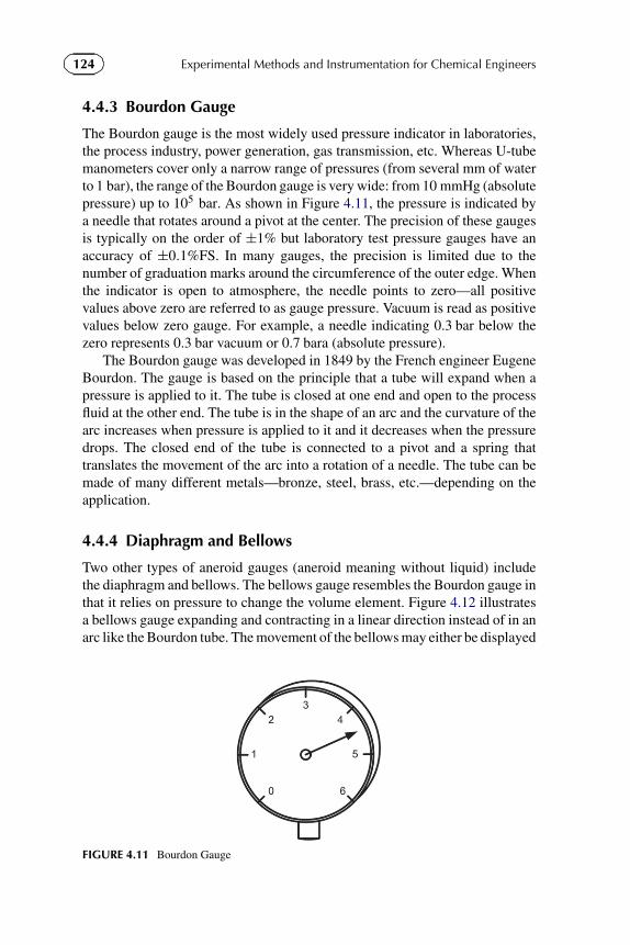
124 Experimental Methods and Instrumentation for Chemical Engineers
4.4.3 Bourdon Gauge
The Bourdon gauge is the most widely used pressure indicator in laboratories,the process industry, power generation, gas transmission, etc. Whereas U-tubemanometers cover only a narrow range of pressures (from several mm of waterto 1 bar), the range of the Bourdon gauge is very wide: from 10 mmHg (absolutepressure) up to 105 bar. As shown in Figure 4.11, the pressure is indicated bya needle that rotates around a pivot at the center. The precision of these gaugesis typically on the order of ±1% but laboratory test pressure gauges have anaccuracy of ±0.1%FS. In many gauges, the precision is limited due to thenumber of graduation marks around the circumference of the outer edge. Whenthe indicator is open to atmosphere, the needle points to zero—all positivevalues above zero are referred to as gauge pressure. Vacuum is read as positivevalues below zero gauge. For example, a needle indicating 0.3 bar below thezero represents 0.3 bar vacuum or 0.7 bara (absolute pressure).
The Bourdon gauge was developed in 1849 by the French engineer EugeneBourdon. The gauge is based on the principle that a tube will expand when apressure is applied to it. The tube is closed at one end and open to the processfluid at the other end. The tube is in the shape of an arc and the curvature of thearc increases when pressure is applied to it and it decreases when the pressuredrops. The closed end of the tube is connected to a pivot and a spring thattranslates the movement of the arc into a rotation of a needle. The tube can bemade of many different metals—bronze, steel, brass, etc.—depending on theapplication.
4.4.4 Diaphragm and Bellows
Two other types of aneroid gauges (aneroid meaning without liquid) includethe diaphragm and bellows. The bellows gauge resembles the Bourdon gauge inthat it relies on pressure to change the volume element. Figure 4.12 illustratesa bellows gauge expanding and contracting in a linear direction instead of in anarc like the Bourdon tube. The movement of the bellows may either be displayed
FIGURE 4.11 Bourdon Gauge

125Chapter | 4 Pressure
Bello
ws
Dis
plac
emen
t
Pressure
Spring Bellows
Connection to indicator
FIGURE 4.12 Bellows Gauge
FIGURE 4.13 Diaphragm
mechanically with a needle or converted to an electrical signal. Because of therelatively large displacement, it is unsuitable for transient measurements.
The diaphragm gauge, on the other hand, has a low mass and a smalldisplacement, which makes it ideal for transient applications. It is essentially athin disk separating two regions as shown in Figure 4.13. When a pressureis applied to one side, the disk deforms elastically. The displacement isproportional to the applied pressure differential and can measure differentialsas low as 1 Pa (approximately 0.01 Torr). The range and sensitivity may beincreased by corrugating the disk but in this case a mechanical device isgenerally used as the sensing element. Otherwise, the deformation may besensed with a strain gauge, which is a device bonded to the surface of thediaphragm. The deformation of the diaphragm causes a change in the electricalresistance of the strain gauge, which is measured with a Wheatstone bridge.
The deformation of the diaphragm depends on the physical geometry of thegauge as well as on the properties of the material of the disk. An important design

126 Experimental Methods and Instrumentation for Chemical Engineers�
�
�
�
TABLE 4.4 Physical Properties of Materials
Material E, GPa G, GPa ν ρ, kg m−3
Carbon steel 200 79 0.29 7760
Stainless steel 190 73 0.31 7760
Nickel steel 200 76 0.29 7760
Monel 179 66 0.32 8870
Inconel 214 79 0.29 8590
Cast iron 100 41 0.21 7200
Aluminum alloys 70 27 0.33 2720
Beryllium copper 124 48 0.29 8310
criterion of the diaphragm is that the maximum allowable displacement, ymax(mm), should be no more than one-third the thickness, t (mm). The displacementis calculated according to the following equation:
y = 3�P
16Et3 r4(1 − ν2), (4.23)
where r is the radius of the diaphragm (mm, E is the modulus of elasticity(Young’s modulus) and ν is Poisson’s ratio.
Table 4.4 summarizes the physical properties of common metals used fordiaphragms. Young’s modulus is a measure of the stiffness of elastic materialsand is defined as the ratio of stress (uniaxial) versus the strain (uniaxial), i.e. theratio of the change in length of an elastic material as a function of a tensile orcompressive load. The Poisson’s ratio is a measure of a material’s tendency tocontract under a tensile load, i.e. the contraction in the direction normal to thedirection in which the material is stretched. The symbol for the shear modulusof elasticity is G.
Example 4.8. Calculate the thickness of a diaphragm to measure a differentialpressure of 10.0 kPa in air at 1.00 atm and 20.0 ◦C. The membrane is made ofstainless steel and has a diameter of 1.0 in.
Solution 4.8. The properties of stainless steel are given in Table 4.4:
E = 200 GN m−2 = 200 × 109 N m−2,
ν = 0.3,
�P = 10 000 Pa,
D = 1 in · 25.4 mm in−1 = 25.4 mm,
r = D/2 = 12.7 mm.

127Chapter | 4 Pressure
The maximum deflection of the diaphragm should be no more than one-thirdthe thickness:
ymax = 3�P
16Et3 r4(1 − ν2) <1
3t .
Substituting ymax for t/3 and rearranging the expression in terms of thicknessgive:
t4 = 9�P
16Er4(1 − ν2).
So, the thickness to the fourth power is related to the radius to the fourth power:
t4 = 9�P
16Er4(1 − ν2) = 9 · 10 000 Pa
16 · 200 × 109 Pa(12.7 mm)4 · (1 − 0.312)
= 6.61 × 10⁻⁴,
t = 0.160 mm.
4.4.5 Vacuum
The first gauge to measure very high vacuum (low absolute pressure) wasinvented by McLeod in 1874. The gauge is capable of assessing pressuresas low as 10−6 bar or 10−4 Torr. They are still common to laboratories andserve well as calibration tools but they have been largely replaced by electronicvacuum gauges for analytical instruments.
Throughout antiquity, the notion of a vacuum has been abhorred. Greekphilosophers posed the question “How can nothing be something?” The CatholicChurch considered it heretical and against nature in medieval times since theabsence of anything translated to the absence of God. In a practical sense,vacuum in the form of cavitation had restricted the ability to pump greater thanten meters of water—one atmosphere—up until medieval times. Cavitation isthe rapid formation and implosion of voids—localized cavities. However, theRomans in Pompeii had a dual-action suction pump which allowed them topump greater than ten meters of water. Suction pumps were also describedby Al-Jazari in the thirteenth century. The Mayor of Magdeburg (Germany)Otto van Guericke invented the first vacuum pump. He demonstrated the conceptby evacuating the air from two hemispheres: a team of eight horses was attachedto each hemisphere, and they pulled until they could no more. From 1850until 1970 the technology to create a vacuum improved continually—every tenyears, the maximum vacuum produced dropped by an order of magnitude from10−1 mbar to 10−13 mbar during this period.
The suction pressure of vacuum cleaners is about 80 kPa and the pressurein an incandescent light bulb varies from 1 Pa to 10 Pa. The vacuum inintergalactic space is estimated to be equal to 10−22 mbar, which is equivalent to4 molecule m−3. Table 4.5 classifies the different categories of vacuum togetherwith the types of instruments generally used for each type. A single instrument isincapable of covering the full range of 10 mbar vacuum to 10−11 mbar. Severaltypes of gauges are required to cover the range continuously.
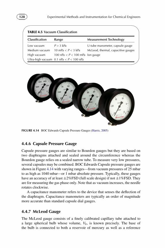
128 Experimental Methods and Instrumentation for Chemical Engineers�
�
�
�
TABLE 4.5 Vacuum Classification
Classification Range Measurement Technology
Low vacuum P > 3 kPa U-tube manometer, capsule gauge
Medium vacuum 10 mPa < P < 3 kPa McLeod, thermal, capacitive gauges
High vacuum 100 nPa < P < 100 mPa Ion gauge
Ultra-high vacuum 0.1 nPa < P < 100 nPa
FIGURE 4.14 BOC Edwards Capsule Pressure Gauges (Harris, 2005)
4.4.6 Capsule Pressure Gauge
Capsule pressure gauges are similar to Bourdon gauges but they are based ontwo diaphragms attached and sealed around the circumference whereas theBourdon gauge relies on a sealed narrow tube. To measure very low pressures,several capsules may be combined. BOC Edwards Capsule pressure gauges areshown in Figure 4.14 with varying ranges—from vacuum pressures of 25 mbarto as high as 1040 mbar—or 1 mbar absolute pressure. Typically, these gaugeshave an accuracy of at least ±2%FSD (full scale design) if not ±1%FSD. Theyare for measuring the gas phase only. Note that as vacuum increases, the needlerotates clockwise.
A capacitance manometer refers to the device that senses the deflection ofthe diaphragm. Capacitance manometers are typically an order of magnitudemore accurate than standard capsule dial gauges.
4.4.7 McLeod Gauge
The McLeod gauge consists of a finely calibrated capillary tube attached toa large spherical bulb whose volume, Vb, is known precisely. The base ofthe bulb is connected to both a reservoir of mercury as well as a reference

129Chapter | 4 Pressure
0
1
2
3
4
5
zc0
1
2
3
4
5
0
1
2
345
FIGURE 4.15 McLeod Gauge: (a) Open to Process Gases; (b) Trapped Process Gas P1;(c) Compressed Pressure Pc
column that leads to the process. Initially, as shown in Figure 4.15, the bulband capillary communicate with the reference column and process so that thepressure throughout equals P1. Mercury is then pumped into the system until itreaches the cut-off point which effectively seals that bulb and capillary from theprocess; the pressure throughout remains at P1. More mercury is pumped intothe system such that the level increases in the bulb and the reference column.It is pumped into the system until the mercury reaches the zero point on thereference column. The height of the gap in the capillary, zc, represents themercury level difference on the reference column and thus the hydrostatic headin the capillary, Pc.
The volume of gas in the capillary, when the mercury reaches the zero pointon the reference column, is equal to the product of the cross-sectional area andthe gap distance, X A,czc.
According to Boyle’s law, as the volume decreases, the pressure increasesproportionately. Therefore, we can equate the pressure and volume in thecapillary when the mercury reaches the cut-off point to that in the capillary:
P1(Vb + Vc) = Pc X A,czc, (4.24)
where Vc is the capillary volume and Pc is the capillary pressure.Therefore, the process pressure is expressed as a function of the capillary
pressure and volumes:
P1 = PcX Azc
Vb + Vc. (4.25)
The gap distance in the capillary, zc (the hydrostatic head of mercury),equals the difference in the capillary pressure and the process pressure (allunits in mmHg):
zc = Pc − P1. (4.26)

130 Experimental Methods and Instrumentation for Chemical Engineers
By design, Vb � Vc and as a consequence, Pc � P1. Therefore, theexpression relating the process pressure to geometry and capillary pressurebecomes:
P1 = X A
Vbz2
c . (4.27)
Example 4.9. Calculate the gap distance of a McLeod gauge measuring apressure of 0.400 Pa. The bulb volume is 15.0 cm3 and the diameter of thecapillary is 0.300 mm.
Solution 4.9.
P1 = 0.400 Pa · 760 mmHg/101 325 Pa = 0.00300 mmHg,
zc = ?
P1 = Xah2
VB,
h =√
P1VB
Xa=√
0.00300 mmHg · 15 000 mm3
π4 0.300 mm)2
= 25.2 mm.
4.4.8 Pirani Gauge
The Pirani gauge is based on heat transfer and thermal conductivity and has awide operating range—from atmospheric to 10−4 mbar. A filament (platinumor tungsten) is placed in the measuring chamber and is connected to an electricalcircuit (Wheatstone bridge). The circuit can be operated such that the wire ismaintained at a constant temperature or so that it heats up or cools down with theoperating pressure. When the pressure is high, there are more frequent collisionsbetween molecules and the wire that cause the temperature to drop. Conversely,when the pressure is low, the wire temperature will be high. The resistance ofthe wire is proportional to its temperature. The thermocouple gauge is basedon the same principle as the Pirani gauge except that the temperature of thefilament is monitored by a thermocouple. The useful range of the thermocouplegauge is somewhat lower at between 1 mbar and 10−2 mbar.
4.5 PROCESS EQUIPMENT AND SAFETY
Pressure is measured at the exit of most vessels, at the discharge ofpumps, inlet and outlet of compressors, and flow meters, along columns—distillation, extraction, reactors—sample lines and analytical equipment.Operating pressure has a significant impact on vessel design, metallurgy,control and operation. At moderate pressures (between 1 barg and 20 barg),the overall investment costs may be relatively insensitive to pressure. For gassystems, higher pressures result in smaller vessels, pipes, control valves, flow

131Chapter | 4 Pressure
PI PIS
FIC
MFC
PI
PI
MFC
FIC
SPI
ATO
ATCON-OFF
ON-OFF
FILTER
FIGURE 4.16 Elements of a P&ID to Feed Air from a Compressor and N2 from a Cylinder
meters, etc. However, beyond 2 bara, compressors are required and cost anorder of magnitude more than blowers and fans. Safety precautions and controlsystems must be more robust at higher pressures. Moreover, higher-grade steelmay be required to conform to vessel code standards. With respect to carbonsteel, 304SS and 316SS are approximately three times more expensive, whileMonel and Titanium are between 5 and 10 times the cost. Besides the type ofmetal, investment cost depends on vessel weight, fabrication cost, complexity aswell as operating pressure. The vessel wall thickness, t, from which the weightis derived, is calculated according to the following equation:
t = Pr
2SE + 0.4P, (4.28)
where r is the radius (mm), S is the maximum allowable stress (psi) (e.g.S = 18 800 psi for SA-516 grade 70), and E is the weld efficiency (0.95for radioagraphed first-class vessels and 0.6 for nonradiographed third-classvessels).
Figure 4.16 is a process flow diagram of the instrumentation for nitrogenand air leading to a reactor. Air is compressed then filtered and the dischargepressure is measured. Following the discharge of the compressor is an on-off valve and two check valves in series to prevent backflow of gas to thecompressor. (Reliability of one-way valves is poor and so two have been placedin the line. Dust, oil, or other debris will block the seating of the valve and forthis reason redundancy is recommended.) After the one-way valves, there is apressure indicator and a ball valve to maintain the pressure at a certain level atthe discharge of the compressor. An air-to-on (ATO) solenoid valve and a massflow controller come after the needle valve: if electricity is lost, the solenoidvalve automatically closes. Flow meters are calibrated at specified pressures andthus a needle valve is placed downstream of the meter plus a pressure gauge.

132 Experimental Methods and Instrumentation for Chemical Engineers
InstrumentProcess
Capped (or flanged)drain connection
Capped (or flanged)test connection
FIGURE 4.17 Typical Line Configuration for Process Instrumentation
The configuration shown in Figure 4.17 is recommended to connect aninstrument to a process. The instrument line leads to a four-way connector;one line goes to the process, another to the vent (or drain), and a third toa test line. Each of the three lines has a valve to isolate the line from theinstrument. During normal operation, the valves to the vent and test line (alsocapped) are closed and the line leading to the process is open. To calibrate theinstrument (or replace/service it), the process line is first closed and the ventline is opened to evacuate the fluid and to drop the operating temperature. Ifthe instrument is to be calibrated, the cap is removed, the valve is opened,and the line to the vent is then closed. To bring the line back on service,the test-line valve is closed and capped. The vent valve is opened, whichdrops the line pressure to atmospheric and then it is closed. Finally, thevalve to the process line is opened. In some cases, the lines may be purgedin order to clear the lines of any potential contaminates (like oxygen forexample).
In many cases, opening and closing the vent lines must be done carefully toreduce sudden changes in pressure that could destroy the instrument. To bringthe instrument back on service, for example, a secondary line may be attachedto the vent line to pressurize the instrument slowly. The line may beoverpressurized so that when the valve to the process line is opened, the purgefluid flows into the process instead of process fluid entering the instrument line.
4.5.1 Pressure Regulator
Instrumentation in the nitrogen line is similar to that of the air line. A gaugewith a range of up to 4000 psig measures the cylinder pressure. It is an integralpart of the pressure regulator that drops the line pressure closer to the desiredoperating pressure to maintain the line at safe and operable value. Often it willbe set at 100 psig to 200 psig, which is measured by the second gauge on theregulator. Pressure regulators are specialized valves that interrupt flow when the

133Chapter | 4 Pressure
line upstream drops below the set pressure: it will shut off when the cylinderpressure drains to the set point pressure. Two-stage regulators are common forgas cylinders, as is the case for nitrogen.
Check valves are infrequent on inert gas lines since there is no inherentsafety risk if a hydrocarbon (or oxygen) were to flow back to the regulator.Backflow of hydrocarbon to an oxygen cylinder—or vice versa—presents aserious hazard.
As opposed to the air line, the nitrogen line has an air-to-close solenoidvalve (ATC). In the case of an emergency, it is preferable to sweep thelines with an inert gas to reduce the possibility of forming a flammablemixture.
The air line and nitrogen line meet at a four-way valve. The valve has twoentrances and two exits. One exit goes to the reactor and the other goes to a vent.To measure the hydrodynamics of the reactor—the gas flow pattern—the valveposition is such that nitrogen sweeps the reactor. When the valve is switched,the air goes to the reactor and the nitrogen exits the vent. The oxygen in the air isanalyzed at a high frequency and the signal is used to interpret the flow pattern orany flow abnormalities such as bypassing. Note that when the reactor and ventare open to atmosphere, the operating pressure equals the barometric pressureand this varies as much as 6% throughout the year with daily fluctuations of asmuch as 3%.
4.5.2 Back Pressure Regulator
When the valve switches from nitrogen to air, the flow of gas will changeabruptly if the vent line and reactor line are inadequately equilibrated; thepressure at both exits of the four-way valve must be equalized. This maybe accomplished by a back pressure regulator. Whereas a pressure regulatorreduces the supply pressure at the inlet to a lower pressure at the outlet, aback pressure regulator throttles the flow downstream to maintain the inletpressure. A needle valve or a back pressure regulator is required at the ventline to match the pressure across the reactor, process lines, and analyticalequipment.
4.5.3 Relief Valves
Back pressure regulators provide steady-state control; relief valves provideon-off protection from overpressure or vacuum conditions. When the setpressure threshold is exceeded, the valve opens either to atmosphere or toan auxiliary line (where the fluid may go to a flare or storage tank or evento recycling). Once the vessel pressure drops to a predetermined pressure, thevalve reseats. The difference in pressure between when the valve relieves andwhen the valve reseats is referred to as the blowdown; it is typically 2–20%lower than the relief pressure.

134 Experimental Methods and Instrumentation for Chemical Engineers
FIGURE 4.18 Vessel Failure Due to Vacuum
4.5.4 Rupture Disk
Most pressure vessels require rupture disks for which designs are specifiedaccording to ASME or other international standards codes. They may protectfrom either overpressure or vacuum conditions. It is composed of a membranethat will instantaneously fail (within milliseconds) at a specified differentialpressure. Figure 4.18 shows a horizontal vessel that failed because it was poorlyvented or due to a failure in the rupture disk.
Example 4.10. Methanol from a 10 m3 reservoir at 20 ◦C is pumped to a railcar for shipment. The total volume of methanol in the reservoir is 9 m3 and thevapor space is blanketed with nitrogen at a pressure of 1.2 bara:
(a) Calculate the vacuum pressure in the vessel when 1 m3 of methanol remainsin the reservoir (assuming the vent line was not opened, the rupture diskfailed, and atmospheric pressure is 1 bar).
Solution 4.10. As a first approximation, assume that the methanol volatilityis negligible, then:
P1V1 = P2V2,
P2 = P1V1
V2= 1.2 bara
1 m3
8 m3 = 0.15 bar.
Vacuum pressure is the difference between atmospheric pressure and absolutepressure:
Pvac = 1 bar − 0.15 bar = 0.85 bar.

135Chapter | 4 Pressure
FIGURE 4.19 Burst Pipe
4.5.5 Pressure Test
The design, fabrication, operation, and inspection of pressure vessels and linesare strictly regulated by engineering agencies such as the ASME (AmericanSociety of Mechanical Engineers). The legal codes are very specific withrespect to the materials of construction, wall thickness, design allowances, andoperating conditions. Several tests may be used to verify the integrity of thevessel, welds, fittings, and ancillary equipment. They may be carried out atpressures lower than the specified operating pressure or at substantially higherpressures. Buried gas and oil pipelines are tested at 125% of the maximumoperating pressure (MAOP). Some codes require vessels to be tested at 150%MAOP.
Many countries enact legislation regarding the frequency of testing theintegrity of pressure vessels. Gas cylinders (high pressure) are generally testedevery two years while fire extinguishers might be tested on a frequency of everyfive to ten years.
Generally, water or another incompressible fluid, like oil, is preferred overgases for pressure testing (Saville et al., 1998). If the vessel fails at high pressure,a sound wave (loud bang) may develop. When using a compressible gas, a shockwave (a pressure wave propagating at supersonic speeds) can be generated. Anadditional hazard in both cases is the possibility of forming high-speed missiles.Figure 4.19 is a picture of a ruptured pipe: the pipe had been mislabelled andwas installed on a steam line at a higher pressure than was specified for the typeof metal.
4.5.6 Leak Test
Leak testing is not only mandatory for testing pressure vessels, it isrecommended for all process lines and analytical equipment. Besides the

136 Experimental Methods and Instrumentation for Chemical Engineers
FIGURE 4.20 Leak Test of a Glass Joint
obvious safety hazards of leaking gases or liquids, very small leaks on thelines leading to pressure gauges may have a profound effect on the recordedsignal. In the laboratory, the most common technique to detect leaks is to bathethe outer surface of the connector with soapy water. Figure 4.20 shows a verylarge bubble forming on the ball joint connecting a quartz reactor to the feedline. Large bubbles are indicative of large gas velocities whereas small bubblesrepresent slow leak rates. Large bubbles are obvious immediately whereas smallbubbles might take some time before they appear. Bubbles can also foam. Attimes, soapy water is insufficient to detect leaks and in these cases a verysensitive detector may be used. These leak detectors are described in the sectionconcerning gas chromatography and are explained in Chapter 8.
4.6 EXERCISES
4.1 Derive an expression for the gas constant, R, as a function ofBoltzmann’s constant based on the kinetic theory of gases.
4.2 Calculate the temperature, Vrms, and concentration of 1 mole of O2 and1 mole of H2 in a one L flask at 1 atm and 10 atm pressure.
4.3 What is the partial pressure of oxygen on the summit of K2 (elevation8611 m)?
4.4 A reservoir 1 m in diameter open to atmosphere contains 10 m3 ofwater at 12 ◦C. The barometric pressure is 770 mmHg. Calculate theabsolute pressure at the bottom of the reservoir.
4.5 A U-tube manometer is filled with mercury at a specific gravity of 13.6to measure the pressure of air exiting a pipe. The low pressure end of thepipe is open to atmosphere at a pressure of 99.2 kPa. The differentialheight of the manometer is 20.5 cm at 25 ◦C. What is the pressure inthe pipe?

137Chapter | 4 Pressure
4.6 A mass spectrometer (MS) is an analytical instrument that determinesthe composition and concentration of compounds—mixtures of gases,liquids, or solids. A sample is ionized to form charged moleculesor fragments and the mass-to-charge ratio (m/z) is then analyzed.Most mass spectrometers operate at 10−6 Pa to minimize collisionswith other molecules. Dual pumps are required. The first brings thepressure down to 0.1 Pa while the second brings it down to the operatingpressure:
(a) Calculate the number of molecules in an MS vacuum chamberoperating at 10−6 Pa (V = 2.0 l,T = 25 ◦C).
(b) The New York City meteorological service reports a barometricpressure of 30.30 inHg. The pressure gauge after the first pumpindicates a vacuum of 760.1 Torr. Is the pump operating correctly?
(c) If the instrument were located in Albany at an altitude of99 m, would your conclusion in (b) change? (Note that themeteorological service corrects the barometric pressure to sealevel.)
4.7 The level of oil in a reservoir is measured with a U-tube manometer(see Figure Q4.7. The pressure at the top of the liquid is 2.5 psig.The barometric pressure at sea level is 780 mmHg. The reservoir islocated at Machu Pichu at an elevation of 2450 m. The manometercontains mercury (ρHg = 13 600 kg m−3) and the density of the oil is865 kg m−3:
Oil
Air
Patm
h2
h1
2'
FIGURE Q4.7 Machu Pichu Oil Reservoir
(a) What is the atmospheric pressure at Machu Pichu in mbar?(b) Calculate the height of the oil in the reservoir (h1)when the height
in the manometer (h2) is equal to 1.45 m.
138 Experimental Methods and Instrumentation for Chemical Engineers
(c) What is the uncertainty in the measure of h1 if the uncertainty inthe measure of h2 is 1.0 cm?
(d) You decide to replace the U-tube manometer with a diaphragm.What would be the ideal diameter for the reservoir if the maximumheight, h1, is 15 m? The diaphragm is made of steel (E =190 GPa, μ = 0.29, and thickness of 0.07 mm).
4.8 A U-tube manometer measures the pressure differential of air in a pipeoperating at 20 MPa and 22 ◦C. The fluid in the manometer is a 50/50(volumetric) mixture of water and glycerine. C. Abou-Arrage
(a) Calculate the weight fraction and density of the manometer fluidknowing that the mixture volume contracts thereby increasing thedensity according to the following relationship:
ρmix = ρthγ,
where:
ρth = ρgl
x − (1 − x)ρgl/ρH2O,
γ = 1 + 0.0283x(1 − x2),
and ρgl equals 1.262, ρH2O is 1000, and x is the mass fraction ofglycerine.
(b) What is the pressure differential for a differential height of 124 mm(in ψ) with a 50/50 mixture of glycerine and water as the fluid inthe manometer.
(c) How much would the pressure drop change with pure water? Withpure glycerine (and the same 124 mm differential height)?
4.9 A transducer is made of aluminum with a Poisson’s ratio of 0.35and a modulus of elasticity of 69 000 MPa. Its diameter is 1 cm. Fora diaphragm that is 0.265 mm thick, what is the maximum pressuredifferential that it can measure? If the thickness is reduced by a factorof 5, what pressure can it measure?
4.10 The temperature of skating rink ice is maintained at −7 ◦C bycirculating a mixture of water and ethylene glycol underneath the ice. Itis important to control the composition of the mixture and samples aretaken from time to time. A simple technique to quantify the compositionis to measure the density, from which the composition may be inferred.Table Q4.10 summarizes voltage measurements for different liquidlevels in a U-tube manometer of the sample. The calibration curverelating the pressure and voltage is given by:
P = 0.924V + 0.800,

139Chapter | 4 Pressure
where P is the pressure (kPa) and V is the voltage (mV). Assumethat the densities of water and ethylene glycol are 1000 kg m−3 and1132 kg m−3, respectively. F.-X. Chiron�
�
�
�
TABLE Q4.10 Pressure Voltage Readings as a Function of Liquid Level
Level (mm) Pressure Transducer Voltage (mV)
21 −0.636
129 0.541
354 3.030
583 5.519
(a) Based on the measurements, calculate the weight percent ofethylene glycol.
(b) The target composition is 48 wt.% ethylene glycol. To reach thisvalue, should water or ethylene glycol be added?
(c) What is the mass and volume of liquid required if the total volumein the reservoir equals 900l?
4.11 The summit of the mountain shown in Figure Q4.11 reaches an altitudeof 3648 m (Point A). The lake is 20 m deep and is situated at analtitude of 1097 m (Point B). Point D is situated at a depth of 150 mbelow the surface of the water. Note that ρair@20 ◦C = 1.20 kg m−3,
ρocean = 1030 kg m−3, and ρlake = 1000 kg m−3. C. Mathieu
FIGURE Q4.11 Pressure at Different Elevations (Patience et al., 2011)

140 Experimental Methods and Instrumentation for Chemical Engineers
(a) Determine the absolute pressure at Points A,B,C , and D.(b) If the uncertainty in the depth of the ocean is ±10 m and that of
the density of water is ±10 kg m−3, what is the uncertainty in theabsolute pressure at Point D?
4.12 An inclined U-tube manometer is filled with water as the measuringfluid. The vertical leg is connected to the upstream of a venture meterand the downstream leg is at an angle of 30◦ with respect to thehorizontal. The ruler has marks at intervals of 1 mm:
(a) Calculate the uncertainty in the pressure in mmH2O if theuncertainty in the angle is ±3◦.
(b) Calculate the pressure differential and uncertainty if thedisplacement of the fluid in the inclined leg reaches a distanceof 1.110 m.
4.13 As shown in Figure Q4.13, a U-tube manometer measures the pressuredrop of water in a pipe. If the height difference in the two legs ofthe manometer filled with mercury is 15.2 cm, what is the pressuredifference between points A and B?
Hg
BA
15.2 cm
FIGURE Q4.13 U-Tube Manometer for Gas Phase Streams
4.14 A U-tube manometer is built with one end open to atmosphere as shownin Figure Q4.14. Oil, with a density of 0.750 kg m−3, flows in the pipeand mercury is charged to the U-tube:
(a) What is the pressure in the pipe if the difference in elevation of themercury is 340 mm and the difference between the height of thelower end of the pipe and the top of the mercury is 1.200 mm?
(b) What is the pressure if the mercury level increases by 10.0 cm?
4.15 In the eighteenth century, the Prince of Conde undertook renovations forthe castle of Chantilly and built canals and fountains. The centerpiece of

141Chapter | 4 Pressure
Hg
0.34 m
1.2 m
FIGURE Q4.14 U-Tube Manometer for Liquid (Low Pressure) Streams
the work was a fountain with a volumetric flow rate of 1 m3 h−1 capableof projecting water to a height of 10 m. Water for the fountain wasavailable from the Oise River to the west of the castle (at an elevationof 40 m above sea level) and the Nonette River to the east 105 m abovesea level). The castle is at an elevation of 70 m. B. Carrier
(a) Calculate the absolute pressure of the water at the base of thefountain.
(b) Which of the two rivers should serve as the source for the fountain?(c) To avoid the use of pumps, the Prince’s architect, Le Nôtre, built a
reservoir upstream at an elevation sufficient to project the water andto compensate for the pressure loss due to friction. If the frictionloss equals 50% of the total head required, at what elevation shouldthe reservoir be built?
(d) If the architect built the reservoir at a distance 40% further awayat an elevation of 90 m higher, and the volumetric flow rateincreased by 20%, calculate the height of the fountain. Note thath f = u2
2g
( LD · const.
).
4.16 You wish to check your electronic altimeter with two portable U-tubemanometers closed at one end (Figure Q4.16). The vertical height ofthe manometer is 0.50 m and you fill one with mercury and the otherwith water at sea level. Note that ρHg = 13 600 kg m−3, ρH2O =1000 kg m−3, g = 9.81 m s−2. J. Fortin
(a) What is the uncertainty in the height and pressure measurement?(b) What is the maximum altitude that can be read with the mercury
U-tube?(c) What is the maximum altitude that can be read with the water
U-tube?

142 Experimental Methods and Instrumentation for Chemical Engineers
=10mm
FIGURE Q4.16 Portable U-Tube Manometer Closed at One End
4.17 A spring type diaphragm pressure transducer is made of carbon steelto measure a pressure differential of 1000 psi. The diameter of thediaphragm is 0.5 in. Calculate the thickness of the diaphragm, in mm,so that the maximum deflection is less than one third its thickness.
4.18 The reservoir of a McLeod has a volume of 15 cm3 and its capillarydiameter is 0.3 mm. Calculate the height of mercury in the capillary ata pressure of 4 Pa.
4.19 A manometer contains an unknown liquid. To identify the liquiddensity, air pressure is applied at one end of the manometer andit is measured with a transducer. Table Q4.19 gives the reading ofthe transducer together with the corresponding height differential ofthe manometer. The relationship between the transducer reading andpressure (in psi) is given by:
P = 87.0V − 307.
(a) Calculate the pressure differential corresponding to eachmeasurement (in kPa).
(b) Identifythe unknown liquid. Note that ρwater = 1000 g l−1, ρacetone =790 g l−1, ρglycerine = 1260 g l−1, ρoliveoil = 920 g l−1, andρether = 710 g l−1.
�
�
�
�TABLE Q4.19 Manometer Calibration Measurements
E, mV 4.00 5.00 6.00
�P , cm 16.0 49.7 83.4
4.20 A high pressure manometer is made to measure a pressure differential ofair of up to 14.0 MPa 20.0 ◦C. Supposing the oil in the tube has a specific

143Chapter | 4 Pressure
0.1 m
0.1 m
0.1 m
0.1 mh = ?
FIGURE Q4.21 Mercury Manometer Connected to Multiple Cylinder Tank
gravity of 0.830, calculate the differential pressure corresponding to adifferential height of 135 mm. If the fluid pressure was lowered to3 MPa, how much would the differential pressure change with the samedifferential height?
4.21 A mercury manometer is connected to the bottom of a tank built witha series of cylinders. Each cylinder contains a different substance: oil(SAE 30), water or glycerin. The cylinder diameters are respectively0.40 m, 0.30 m, and 0.20 m. Calculate the height h, shown in FigureQ4.21. C.-G. Castagnola
4.22 What is the pressure at an altitude of 5000 m on Venus?4.23 A 20.0 ± 0.1 mm diameter beryllium copper diaphragm measures
the differential pressure between a column of water and atmosphericpressure on Table Mountain (Cape Town, SA) at an elevation of1086 m. The column of water causes the diaphragm to deflect by0.030±0.001 mm and its thickness is .210±0.003 mm. (a) What is themaximum permissible deflection of the diaphragm? (b) Calculate thepressure drop due to the column of water. (c) How high is the columnof water? (d) What would the deflection of the diaphragm be if thecolumn of water was brought down to Cape Town (at sea level)? (e)What is the uncertainty in the pressure drop. V. Labonté
4.24 Knowing that the gravitational constant may be approximated by thefollowing relationship (in the range of 0–100 km, with Z in m):
g(z) = g − 0.00000303Z .
(a) Derive an exact expression for pressure as a function of elevationin the troposphere.
(b) What is the error in the predicted pressure at an elevation of 1000 mwhen the variation of the gravitational “constant” with elevationis neglected?

144 Experimental Methods and Instrumentation for Chemical Engineers
REFERENCES
Environnement Canada. (n.d.). Pressure measurement. Retrieved 2011, from EnvironnementCanada: <http://www.ec.gc.ca/default.asp?lang=fr>.
Graham, B., Reilly, W.K., Beinecke, F., Boesch, D.F., Garcia, T.D., Murray, C.A., Ulmer, F., "DeepWater: The Gulf Oil Disaster and the Future of Offshore Drilling", Report to the President,National Commission on the BP Deepwater Horizon Oil Spill and Offshore Drilling, January,2011.
Harris, N., 2005. Modern Vacuum Practice, third ed. McGraw-Hill.Haynes, W.M. (Ed.), 1996. CRC Handbook of Chemistry and Physics, 92nd ed. CRC Press.Patience, G.S., Hamdine, M., Senécal, K., Detuncq, B., 2011. Méthodes expérimentales et
instrumentation en génie chimique, third ed. Dept. Chemical Engineering, Ecole Polytechniquede Montréal.
Poling, B.E., Prausnitz, J.M., O’Connell, J.P. 2001. The Properties of Gases and Liquids, 5th ed.,App. A, McGraw-Hill, New York.
Saville, G., Richardson, S.M., Skillerne, B.J., 1998. Pressure Test Safety, HSE Books.
Chapter 5
Temperature
5.1 OVERVIEW
The five senses that everyone recognizes are sight (ophthalmoception),hearing (audioception), taste (gustaoception), smell (oflacception), andtouch (tactioception). Other senses that are less frequently cited includebalance (equilibrioception), acceleration (kinesthesioception), kinestheticsense (proprioception), pain (nociception) and, of course, temperature—thermoception. The receptors in our body sense heat and cold on our skin,but they are also sensitive to infrared radiation. Although the body sensestemperature and changes in temperature, it is unreliable for quantitativemeasurements: many factors are required to constitute a reliable measureincluding reproducibility and a scale—both are lacking with respect to thebody. The skin senses relative temperature—hotter and colder—but the rangeis narrow and unreliable. For example, if you place your left hand in ice waterand your right hand in hot water, then put both hands in lukewarm water, thesensation will be different for each hand.
Although temperature measurement and control is critical in thedevelopment of many processes throughout history, a universally acceptedscale was only developed in the last couple of centuries. Besides agriculture,temperature control and pyrotechnology were the most important developmentsresponsible for the advancement of civilization. Pyrotechnology was used as anengineering tool in the development of prehistoric societies perhaps as far backas 164 000 yr ago (ka) in South Africa (Brown et al., 2009). Fire was used forwarmth, light, and cooking up to 790 ka, as shown in Table 5.1. Evidence of theuse of fire dates back more than twice that at over 1500 ka. The technologicaljump to using fire to alter and improve raw materials is poorly documentedor understood. However, heat treatment of silcrete (a type of rock) to form
Experimental Methods and Instrumentation for Chemical Engineers. http://dx.doi.org/10.1016/B978-0-444-53804-8.00005-8© 2013 Elsevier B.V. All rights reserved. 145
146 Experimental Methods and Instrumentation for Chemical Engineers
tools predominates in multiple sites in South Africa at about 71 ka. The firstevidence of heated silcrete to make tools dates back as far as 160 ka, which isapproximately the same time that the fire-hardening of wood (Thieme, 1997)to make tools and weapons seems to have emerged. Other processes have beendeveloped in which temperature control has been critical, including mundaneapplications like drying wood for firewood or drying malted barley for brewinghops to highly sophisticated and demanding applications including firing clayto make pottery—earthenware, stone wares, and porcelain—or smelting copperand iron ores (Nicholson and Shaw, 2000).
The early applications could be easily achieved with the heat from firein which temperatures are generally less than 600 ◦C such as fire settingfor mining and quarrying (Weisberger and Willies, 2001). The productionof earthen pottery requires temperatures higher than 800 ◦C and high-qualitypottery requires temperatures as high as 1200 ◦C: to achieve and control thesetemperatures in 8000 BC necessitated an understanding of heat transfer, air flow,insulation, time, and temperature! Smelting (copper and iron), glass, cement,and porcelain are processes that were developed subsequently to the majorinnovations required to make pottery (Hummel, 2005).
How did the ancients achieve and control high temperatures for extendedperiods of time in order to make pottery? Modern kitchen ovens typicallyoperate at less than 250 ◦C whereas gas barbecues can reach perhaps as high as400 ◦C. The early use of fire to boil water, cook food, or harden wood wouldhave required temperatures below 200 ◦C. Firing clay in order to make potteryrequires much higher temperatures. To vitrify even low-fire clays requirestemperatures in the vicinity of 1000 ◦C, while the coal bed of a campfire istypically around 600 ◦C it can get as high as 750 ◦C when it glows red hot(Berna et al., 2007).
Pottery requires both a high degree of precision around the temperatureramp as well as extremely high temperatures. In the first stage, “bone dry” clayis heated to drive off adsorbed water trapped in the interstices. If this is donetoo rapidly, steam is generated, which expands and will crack and destroy thepottery. In the second stage (from 300 ◦C to 800 ◦C), carbon and sulfur combust.In the third stage, kaolin clays dehydrate, beginning at 550 ◦C (and continuingup to 900 ◦C).
Al2O3 · 2α-SiO2 · 2H2O573 ◦C−→ Al2O3 · 2β-SiO2 + 2H2O.
At 573 ◦C, the quartz inversion temperature where the α-SiO2 crystal phaseconverts reversibly to theβ-SiO2 phase, the volume changes by 2%. This volumechange can introduce cracks if the temperature on one side of the pottery is muchdifferent from the other side. At 900 ◦C, the clay sinters (the particles begin tofuse together)—fifth stage. In the sixth stage, alumina silicate forms during theprocess of vitrification.

147Chapter | 5 Temperature�
�
�
�
TABLE 5.1 Pyrotechnology and Temperature in History (Prior to 1000 AD)
Year Pyrotechnology Temp. (◦C)
790 ka Demonstrable evidence for the use of fire 200–300
400 ka Fire-hardening wood (for tools andweapons)
<200
70 ka Widespread use of stone tools made fromfire—South Africa
∼ 450
70 ka Smoking animal skins to produce leather <100
50 ka Ground, fired iron oxide producing variouspigments (maybe as far as 400 ka)
300–350
23 ka Baked clay figurine—Venus of Vestonice 300–400
14 ka Pottery vessels 500–800
8800 BC Line-plaster from limestone (quicklime—CaO)
870
8000 BC Ceramic pottery 800–1200
7000 BC Quarrying using fire-setting 600
5500 BC Copper smelting 1084
4500 BC Fire-setting malachite/azurite (copper ores)at Rudna Glava
480
3000 BC Glazed earthenware to reduce porosity
Bread making (adding cold water, hotwater, baking, hot stones, fire oven)
Brewing beer
Steam distillation (essential oilextraction—Frankincense)
100
2500 BC Fire-setting by Chefryn to quarry stone forpyramids
480
2400 BC Glass-making by Akkadians
2000 BC Fire-setting by Egyptians in gold mining 480
1400 BC Stoneware 1200–1300
800 BC Chinese glazed pottery
300 BC Distillation of sea water by Greek sailors 100
200 BC Cement 1450
50 BC Glassblowing—Phoenicia
618 AD Porcelain 1400

148 Experimental Methods and Instrumentation for Chemical Engineers
FIGURE 5.1 Pit Kiln Time-Temperature Profile
Open fires are insufficient to produce a ceramic material. Before brickkilns were developed (mud brick houses were common across the Indus valleybefore 3200 BC), the high temperatures were produced in pit-kilns: a fire wasbuilt in a hole in the ground, clay was placed in the pit and then coveredwith more combustible material, rocks, broken pottery, and dirt to reduceheat losses. Figure 5.1 demonstrates the time-temperature history of a pit-kiln built to produce lime plaster—CaO (Goren and Goring-Morris, 2008;Goren-Inbar et al., 2004) from limestone (CaCO3). The experiment wasconducted by digging a 2.5 m diameter hole 75 mm deep, then filling it with500 kg of limestone and 1 t of fuel—logs, branches, and cow and horse dung.The logs were first placed radially, leaving a 0.5 m diameter circle in the center.Dung and branches were placed between the logs to fill the spaces and limestonepebbles were placed on top of the fuel. Four successive layers were made afterwhich large boulders were placed around the outer perimeter and more boulderswere added to form a dome. The dome in the middle was then filled with looselypacked fuel. As shown in the figure, a maximum temperature of 870 ◦C wasachievable.
5.2 TEMPERATURE SCALES
Achieving high temperature for an extended period of time for earthenware, tosmelt copper or iron and to manufacture cement is a tremendously energy-intensive operation. To produce 250 kg of lime clay (Figure 5.1), 1 t offuel was necessary. Nowadays cement production, which requires calcinationtemperatures of 1450 ◦C, contributes between 2% and 5% of global CO2emissions. It is hard to imagine that ancient civilizations had limited or nomeans of assessing temperature considering the substantial economic impact

149Chapter | 5 Temperature
Temp., °C Cone
1400 Brilliant white 14
1300 White 11
1200 Yellow (white) 5 ½
1100 Yellow-orange 1
1000 Orange 06
900 Red-orange 010
015800
700 018
600 Dark red 021
500 Dull red glow
400 Black
300
200
100
Dull red
Cherry red
FIGURE 5.2 Kiln Firing Chart (For color version of this figure, please refer the color plate sectionat the end of the book.)
for incorrectly firing pottery or making cement. Throughout history, hominidshave recognized the difference between hot and cold, freezing and boiling.Although temperature was not quantitatively measured, it must have beenprecisely controlled. The most obvious means of assessing the energy levelof a fire is by looking at its color. Figure 5.2 shows the kiln firing chart thatrelates color to temperature in Kelvin and a scale used in the pottery industrybased on the deformation of cones.
The first recorded temperature scale was developed by the Greco-Romanphysician Galen around 170 AD. He proposed combining proportions of ice andboiling water to form a scale. The neutral point was equal masses of water andice. There were four degrees above and below this neutral point. Coincidentally,while the temperature scale we now use was being developed, the Englishpotter Josiah Wedgewood proposed a scale above the boiling point of mercury

150 Experimental Methods and Instrumentation for Chemical Engineers
(356 ◦C). The starting point was defined as 580.5 ◦C but the actual startingtemperature was closer to 269 ◦C. The steps were approximately 16.9 ◦C, whichis much lower than the 54 ◦C increments that were originally quoted. By theeighteenth century, as many as 35 temperature scales had been conceived.
Galileo is credited with inventing the first instrument to assess the changein temperature, referred to as a thermoscope. Thermoscopes show changes intemperature but lack a quantitative scale. Jean Rey in 1632 was the first to usethe dilation properties of liquids. In 1641, Ferdinand II, Grand Duke of Tuscany,hermetically sealed alcohol in a glass contraption with graduation marks.
He, together with Prince Leopold of Medici, created the Academia delCimento and in 1667, the academy published five treatises: the first instrumentwas that invented by Fredinand, consisting of a long necked-tube on top of aspherical bulb with 50 increments. The second instrument was similar to thefirst but with 100 increments. The third instrument was much larger and had 200hundred increments. These instruments are commonly referred to as Florentinethermometers.
Hooke (1664) improved on the design with an expanding liquor (a reddyed alcohol) in a tube four feet long that would reach the top in the heatof the summer and approach the bottom at the coldest point in the winter. Hegraduated the stem of the thermomenter by marking zero at the height of thefluid in the stem when the bulb was placed in freezing water. One year later,the Dutch Mathematician Huyghens proposed freezing and boiling water astwo reference points to designate a scale. Fabri, a French Jesuit, constructedan instrument with the zero reference equal to the freezing point of water andselected the highest heat of the summer as the upper reference point. He thendivided the distance between the two points into eight equal parts in 1669. In1701, the Danish Astronomer Romer defined the zero point equal to the freezingpoint of a mixture of water and salt and the boiling point of water was set toequal 60. Newton also developed a temperature scale but rejected using boilingwater as a reference point because it begins to boil at one point and then boilsvehemently at another point. In fact, the temperature of boiling water dependson atmospheric pressure, chemical purity, the shape of the vessel as well as theposition of the thermometer (Sherwood-Taylor, 1942).
Fahrenheit was the first to construct a mercury thermometer (although atleast ten others long before him had tested the use of Hg) and adapted a newscale from Romer’s in 1714. Originally, he used the Florentine scale (−90,0, 90). Then he developed his own scale (0, 12, 24) which was derived fromfoot measurements (Bolton, 1900). Because the graduations were imprecise, headded a factor of 4 to the scale so that it ranged from 0 to 96. The zero point waschosen to be the freezing point of brine; a mixture of ice and water was set toequal 32◦; and the average body temperature was designated as 96◦. (The scalewas later refined such that the boiling point of water equaled 212◦ exactly andthe temperature of melting water was 32◦.)

151Chapter | 5 Temperature
Ferchault de Reaumur de Facheur (1731) used alcohol diluted with 20%water and showed that this mixture expanded from 1000 to 1080 volumesbetween the freezing point and boiling point of water. Thus, his scale variedbetween zero at the freezing point of water and 80 at the boiling point. Aprofessor of astronomy in St. Petersburg, Joseph Nicolas de l’Isle, proposeda scale in which 0 represented the boiling point of water and 150 its freezingpoint. In 1742, A. Celsius—a professor of astronomy—adopted 100 as thefreezing point of water and zero as its boiling point. Shortly thereafter, twoscientists reversed the Celsius scale independently in Uppsala (Marten Stromer)and Lyons (Christin). Up to 18 different temperature scales were used in 1840.In 1900, three scales were in common use but no nation adopted the scale of itsown citizen: English-speaking countries adopted the Fahrenheit scale (German),Germany chose the Reaumur scale, and the Celsius (Swedish) scale as modifiedby Christin of Lyon was popular in France, Belgium, and Switzerland.
Jacques Charles discovered in 1787 that at constant pressure, the volume of agas drops by 1/273 per ◦C, which suggested that gases would disappear if cooledbeyond −273 ◦C. In 1848, Lord Kelvin proposed that molecular translationalenergy and not volume becomes zero at this value. The Kelvin scale assigns thevalue of zero as this point and 273.15 K as the melting point of water. It wasselected as the metric unit for temperature in 1954 and changed from ◦K to Kin 1967. In 1859, William J. Rankin assigned 0 as the thermodynamic absolutezero and 459.67 as the melting point of water.
Table 5.2 summarizes some characteristic temperatures of importantphysical properties. The range is from absolute zero to the temperature of theouter surface of the sun at close to 6000 K
Although the Kelvin scale is the accepted international standard, it isinfrequently used except in scientific articles. Even in journals the Celsius scaleis often used. The Fahrenheit scale remains the official scale in the United Statesand Belize. To convert from ◦C to ◦F:
T◦F = 1.8 T◦C + 32.
Whereas standard pressure has recently been defined by the IUPAC as 1bar, the conditions of the term “standard” have not as of yet been universallyaccepted. In the gas industry, standard conditions (STP) are 1 atm and 60 ◦F(15.6 ◦C). The IUPAC definition of standard temperature is 0 ◦C, whereas someassign 25 ◦C as standard temperature. Its definition of normal temperatureand pressure is 20 ◦C and 1 bar, respectively. Whenever a new instrument—particularly flow meters—is brought into service, the manufacturer’s definitionof STP must be verified to avoid introducing a systematic error.
5.2.1 Wet-Bulb, Dry-Bulb Temperature, Dew Point
A class of process equipment (Unit Operations) of Chemical Engineering isconcerned with either condensing a vapor from a gas stream or saturating a

152 Experimental Methods and Instrumentation for Chemical Engineers�
�
�
�
TABLE 5.2 Characteristic Temperatures
◦C K ◦F
55067 5780 9944 Temperature on the surface of the sun
3410 3683 6170 Melting point of tungsten
1668 1941 3034 Melting point of titanium
1064 1337 1948 Melting point of gold
420 693 787 Melting point of zinc
100 373 212 Boiling point of water
58 331 136 Highest temperature recorded on earth
37 310 98.6 Body temperature
20 293.15 68 Ambient temperature
3.97 277 39 Temperature of water at its maximum density
0.01 273.16 32 Triple point of water
−17.78 255 0 Zero on the Fahrenheit scale
−89 184 −129 Coldest temperature recorded on earth
−219 54 −362 Triple point of oxygen
−259 13.8 −435 Triple point of hydrogen
−273.15 0 −459.67 Thermodynamic absolute zero
gas stream with a vapor—“gas” refers to the non-condensable component ofthe stream and vapor refers to the condensable component. In humidificationand dehumidification operations, water is the vapor component and air is thegaseous component. A saturated gas is one in which the vapor concentration isin equilibrium with the gas. Relative humidity is the ratio of the water partialpressure to the saturated water vapor pressure at the same conditions (100%humidity). The Antoine equation may be used to calculate absolute humidity, asa function of temperature (see Table 4.1), but other more complex and accuratecorrelations have also been proposed.
Note that the partial pressure of water vapor in air at 100% humidity and5 ◦C is much less than at 50% relative humidity and 30 ◦C. This has importantimplications with respect to drying operations; the driving force for evaporationis proportional to the difference between the water vapor pressure and the web-bulb temperature, which is equivalent to what the body would feel when theskin is wet and then exposed to a moving stream of air. It is measured byplacing a damp wick over a liquid-in-glass thermometer and then spinning thethermometer at a high enough rate to simulate an air stream.
The dry-bulb temperature is the thermometer reading in the absenceof humidity and radiation; it is the temperature most often reported bymeteorological agencies. The dew point is the temperature at which the watervapor in the air first begins to condense: the dew point equals the measuredtemperature when air is 100% saturated—100% humidity.

153Chapter | 5 Temperature
5.2.2 Humidex, Heat Index
The sensation of heat is more pronounced when the humidity is high compared toa dry environment at the same dry-bulb temperature. Perspiration (sweat) coolsthe body when it evaporates. The evaporation rate depends on many factors ofwhich the relative humidity is possibly the most important: at 100% relativehumidity, air is saturated with water vapor and so at this condition there is nodriving force to evaporate perspiration from the body. This effect is accountedfor by two scales: in the United States, meteorologists report the Heat Indexwhile in Canada they report the Humidex (Steadman, 1979). The Humidex isbased on the dew point temperature, Tdew and the dry-bulb temperature, T, andis expressed as:
THX = T + 0.5555
(6.11e
5417.7530(
1273.15 − 1
Tdew
)− 10
).
A Humidex of 30 is mildly uncomfortable—it feels like 30 ◦C with nohumidity. A value of 40 is extremely uncomfortable and 45 is dangerous. Heatstroke is probable at values above 54.
This expression was developed when Canada was still officially using theFahrenheit scale and could be simplified by multiplying the constants in thebrackets by 0.5555. Furthermore, there is an inconsistency with respect to thecoefficients—eight significant figures for the coefficient in the exponential andonly two for the value “10”. Clearly two significant figures would be sufficientto communicate the sensation of heat due to humidity.
The Heat Index (Rothfusz, 1990) is rather more complicated and isexpressed as:
THI = −42.379 + 2.04901523T + 10.14333127HR − 0.22475541T HR
−6.83783 × 10⁻³T 2 − 5.481717 × 10⁻² H2R
+1.22874 × 10⁻³T 2 HR + 8.5282 × 10⁻⁴T H2R
−1.99 × 10⁻⁶T 2 H2R .
The variable T refers to the dry-bulb temperature in ◦F and HR is the relativehumidity in %. As with the expression for Humidex the coefficients with10 significant figures are excessive. However, with higher order polynomialexpressions many significant figures are often required: the difference in thecalculated value of THI between the equation above and with coefficients withonly four significant figures is 18 (at 90 ◦F and 80% HR).
5.2.3 Wind Chill Factor
Whereas the Humidex accounts for the effect of humidity on how the bodyperceives temperatures above 20 ◦C, the wind chill factor accounts for theenhanced cooling effect caused by wind. The sensation of temperature depends

154 Experimental Methods and Instrumentation for Chemical Engineers
on various phenomena including the evaporation rate, conduction, convectionand, during sunny days, radiation. The heat lost from the body increases withincreasing wind speed due to higher local convection rates on the skin andaround the body. As in the seventeenth to nineteenth centuries, a world standardto account for the wind chill has yet to be adopted. Since 2001, the weatherservices in Canada and the US report Wind Chill according to the followingrelationship:
TWC = 13.12 + 0.6215T − 11.37V 0.16 + 0.3965T V 0.16,
where T is the dry-bulb temperature in ◦C and V is the wind speed measured ata height of 10 m (km h−1).
5.3 MECHANICAL INSTRUMENTS
According to the second law of thermodynamics, heat flows from a hot bodyto a cold body (unless work is done to reverse the direction). Temperature is anintensive thermodynamic property—unlike length and mass, whose values canonly be compared to a standard—and represents the level of molecular energyof molecules.
Many instruments have been developed to measure the change in molecularenergy and they can be broadly classified as mechanical, electrical, or based onthe detection of electromagnetic waves (infrared and visible light). Although10 000 yr ago the concept of temperature must have been well understood andquantitatively measured (most probably based on color), the first documentedevidence of a device to measure it dates back to around 240 BC. Philo ofByzantium observed that bubbles would escape a tube immersed in water whichwas connected at the other end to a (sealed) hollow sphere when it was placedin the sun. When it was placed in the shade, water would rise into the tube. Heroof Alexandria (10–70 AD) further developed this concept, which later inspiredFludd (English physician, 1538), Galileo (1592), and Sanctorius (1612).
5.3.1 Gas Thermometers
Mechanical-based instruments used to measure temperature are based on thedilation properties of gases, liquids, and solids. The first thermometers werebased on gases. The volume of an ideal gas will change in direct proportion toits temperature (under isobaric conditions). According to Charles’ Law:
T = TrefV
Vref.
Figure 5.3 illustrates the thermoscope of Sanctorius, reproduced from anillustration by Biancani. The long tube is immersed at the bottom in a pool ofwater and at the top by a hollow sphere. When the top sphere is heated, the

155Chapter | 5 Temperature
Capillarystem
Reservoir,bulb
Overflow bulb
FIGURE 5.3 Thermoscope of Sanctorius
volume of gas expands and the liquid level drops. The liquid level increaseswhen the sphere at the top is cooled. Temperature gradients along the tubelength will make a precise measurement of the temperature difference.
The range of a constant-pressure gas thermometer is limited by the volumeof the instrument of the graduated tube recording the change in height of thefluid. High pressure and low pressure ranges may be examined independently bypressurizing the tube. Higher ranges may be achieved with pressure-measuringconstant-volume gas thermometers. For ideal gases, temperature increasesproportionally with pressure at constant volume.
A special case of “constant-volume” gas thermometry is that based on thevapor pressure of a liquid. As the temperature of a solvent is increased, itsvapor pressure increases proportionately over a wide range of conditions. Thetemperature range is limited to temperatures between the boiling point andfreezing point of the solvent and it must also be lower than the critical pointof the fluid. These thermometers are easy to adapt to common experimentalequipment.
The pressure can be measured by a Bourdon gauge or a U-shapedmanometer, as shown in Figure 5.4. In the case of a Bourdon gauge, the volumeis constant and the pressure increases. In the case of a U-tube manometer, thevolume increases with pressure and therefore, may not strictly be considered a“constant-volume” gas thermometer. Although the simplicity of the apparatusis attractive, it is extremely difficult to achieve a high degree of accuracy.
The volume of the solvent immersed in the medium to be measured mustbe much larger than all connecting lines between the pressure instrument andthe solvent. In the case of Figure 5.4, the solvent will condense on all surfacesat temperatures lower than the bath temperature. In fact, the tubing of a U-tube

156 Experimental Methods and Instrumentation for Chemical Engineers
FIGURE 5.4 U-Shaped Manometer Configured to Measure Temperature
should be heated to a greater temperature than that of the bath to minimizecondensation.
Example 5.1. The temperature of the water in a beaker on a hot plateis measured by a “constant-volume” thermometer. The cylindrical body ofthe thermometer is 200 ml. It is connected directly to a Bourdon gauge.The barometric pressure is 750 mmHg. Assume that the following experimentsare conducted rapidly such that the tubing operates isothermally.
(a) What is the temperature of the water if the bourdon gauge reads 1.0 psig?(b) In the second case, 50 ml of ethanol is placed in the body of the thermometer.
What is the pressure recorded on the Bourdon gauge if the temperatureincreases to 55 ◦C?
(c) In the third case, the thermometer is connected to a U-tube manometer ofwhich the total length of tubing (1/4 in. diameter) between the top and thezero point of the manometer is 1m. What is the temperature of the water ifthe differential height in the U-tube is 14 in.? (The cylindrical body containsonly air.)
Solution 5.1a. The Bourdon gauge should be placed as close to the cylindricalbody to minimize the total volume of gas that remains unheated. Assumingthat this dead volume is negligible, Amontons’ Law of Pressure-Temperatureapplies:
P1/T1 = P2/T2.
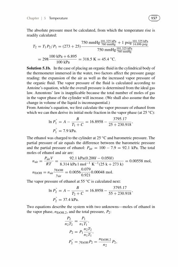
157Chapter | 5 Temperature
The absolute pressure must be calculated, from which the temperature rise isreadily calculated:
T2 = T1 P2/P1 = (273 + 25)750 mmHg 101.325 kPa
760 mmHg + 1 psig 101.325 kPa14.696 psig
750 mmHg 101.325 kPa760 mmHg
= 298100 kPa + 6.895
100 kPa= 318.5 K = 45.4 ◦C.
Solution 5.1b. In the case of placing an organic fluid in the cylindrical body ofthe thermometer immersed in the water, two factors affect the pressure gaugereading: the expansion of the air as well as the increased vapor pressure ofthe organic fluid. The vapor pressure of the fluid is calculated according toAntoine’s equation, while the overall pressure is determined from the ideal gaslaw. Amontons’ law is inapplicable because the total number of moles of gasin the vapor phase of the cylinder will increase. (We shall also assume that thechange in volume of the liquid is inconsequential.)From Antoine’s equation, we first calculate the vapor pressure of ethanol fromwhich we can then derive its initial mole fraction in the vapor phase (at 25 ◦C):
ln P◦1 = A − B
T1 + C= 16.8958 − 3795.17
25 + 230.918,
P◦1 = 7.9 kPa.
The ethanol was charged to the cylinder at 25 ◦C and barometric pressure. Thepartial pressure of air equals the difference between the barometric pressureand the partial pressure of ethanol: Pair = 100 − 7.9 = 92.1 kPa. The totalmoles of ethanol and air are:
nair = PairV
RT= 92.1 kPa(0.200l − 0.050l)
8.314 kPa l mol−1 K−1(25 k + 273 k)= 0.00558 mol,
nEtOH = nairyEtOH
yair= 0.0056
0.079
0.9210.00048 mol.
The vapor pressure of ethanol at 55 ◦C is calculated next:
ln P◦2 = A − B
T2 + C= 16.8958 − 3795.17
55 + 230.918,
P◦2 = 37.4 kPa.
Two equations describe the system with two unknowns—moles of ethanol inthe vapor phase, nEtOH,2, and the total pressure, P2:
P2
n2T2= P1
n1T1,
P2 = P1n2T2
n1T1,
P◦2 = yEtOH P2 = nEtOH,2
n2P2,

158 Experimental Methods and Instrumentation for Chemical Engineers
wheren2 = nEtOH,2 + nair.
We can solve for the total moles of ethanol in the vapor phase by substitutingthe expression for the total pressure (from the ideal gas law) into the expressionfor the vapor pressure:
P◦2 = nEtOH,2
n2P1
n2T2
n1T1,
from which
nEtOH,2 = n1P
◦2
P1
T1
T2= 0.00606
37.4
100
298
328= 0.00206 mol.
With the total number of moles of ethanol in the vapor phase together with themoles of air, the pressure is now calculated:
P2 = nEtOH,2 + nair
nEtOH,2P
◦2 = 0.00206 mol + 0.00558
0.0020637.4 kPa = 139 kPa.
This pressure is substantially greater than when only air is placed in the cylinderand thus the precision is superior. However, the design of the thermometer ismuch more difficult due to the possibility of vapor condensation in the Bourdontube or in the tubing connecting the two. Furthermore, the lines connecting thetube to the gauge should also be completely immersed in the measured fluid toreduce ambiguity with respect to possible temperature variations.
Solution 5.1c. The situation with the U-tube manometer is a little morecomplicated. There are two systems that are coupled. The cylinder immersedin the water is a constant-volume vessel. The pressure and temperature willincrease and there will be an outflow of moles to the tube. The tube is operatedisothermally and the volume increases as the liquid level drops in the U-tube.The pressure in the cylinder equals the temperature in the tubing. The conditionsin the cylinder before heating are:
P1 = 750 mmHg101.325 kPa
760 mmHg= 100 kPa,
Vc = 200 mm,
T1 = 25 + 273 = 298 K,
nc,1 = P1Vc
RT1= 100 kPa200 × 10−31
8.314 kPa l mol−1 K−1298 k= 0.008 07 mol.
The pressure and temperature in the tubing are the same as in the cylinder. Thenumber of moles and volume are:
nt,1 = P1Vt,1
RT1= 100 · 31.7 × 10−3
8.314 · 298= 0.00128 mol.

159Chapter | 5 Temperature
As the cylinder heats up, the pressure increases and the gas expandscoincidentally such that the total number of moles in the cylinder decreases.The decrease in the number of moles in the cylinder corresponds to the increasein moles in the tubing, �n, which equals the volume displacement of themanometer fluid. We assume that the tubing temperature is constant, but thepressure increases, which is calculated based on the displacement of the fluidin the manometer:
Vt,2 = Vt,1 + �V = V1 + π
4d2h
= 31.7 + π
4
(0.0254
4
)2
· 0.0254 · 14 × 106 = 43.0 ml,
P2 = P1 + �P = P1 + ρgh = 100
+1000 · 9.8 · 0.0254 · 14/1000 = 103.48 kPa.
Again from the ideal gas equation, the total number of moles in the tube maybe calculated including the volume expansion and the increased pressure:
nt,2 = P2Vt,2
RT1= 103.48 · 43.0 × 10−3
8.314 · 298= 0.00180 mol.
So, the number of moles exiting the cylinder and entering the tubing is thedifference between the moles in the tubing before and after heating:
�n = nt,2 − nt,1 = 0.00180 − 0.00128 = 0.00052 mol.
For the conditions in the cylinder for which we wish to calculate the temperature,we can again apply the ideal gas equation since all of the conditions are nowdefined:
nc,2 = nc,1 − �n = 0.00807 − 0.00052 = 0.00755 mol,
T2 = P2V2
nc,2 R= 103.48 · 200 × 10−3
0.00755 · 8.314= 330 K = 57 ◦C.
5.3.2 Liquid Thermometers
Liquid thermometers are the most common instrument employed to measureatmospheric temperature. They have an excellent range and can measuretemperatures from as low as −200 ◦C to above 600 ◦C. Similarly to gasthermometers, they are based on the dilation properties of liquids when subjectto changes in temperature. Many liquids have been used to measure temperatureincluding water, alcohols, mercury, paraffins, and aromatics.
The liquid-in-glass thermometer consists of a bulb containing a reservoirof fluid. A stem, connected to the bulb, contains a capillary tube on the orderof less than 0.5 mm in diameter. As the bulb is heated or cooled, the fluid in

160 Experimental Methods and Instrumentation for Chemical Engineers
the capillary will rise or fall. A scale is etched along the stem to represent thetemperature. Often, a small bulb at the other end of the capillary is added forsafety: if the bulb is accidentally overheated, excess fluid will accumulate in thisregion, thus reducing the risk that the thermometer bursts. To improve accuracy,the stem is notched to indicate the height to which the thermometer should beimmersed in the fluid. The fluid and glass expansion properties are different,which must be accounted for in the calibration of the thermometer.
Among the first commercial thermometers were those manufactured byFahrenheit with mercury. The advantages of mercury over most other fluidsinclude its very low vapor pressure, excellent temperature range—from −38 ◦Cto 650 ◦C—and short response time. Short response time is a convenient,if not important, factor with respect to medical applications. AlthoughSanctorius’ “thermoscope” was used for medical purposes up until 1866,clinical thermometers were 300 mm long and took 20 min to record a patient’stemperature. In 1866, Albutt invented a thermometer half that length thatrequired only 5 min (Adler, 1974).
Despite the advantages of Hg, alcohol thermometers are replacing mercuryas the liquid of choice principally driven by safety considerations. Mercuryis toxic. Moreover, when the thermometer breaks, mercury beads into smallspheres making it difficult to clean, which increases both its environmentaland health hazard. Disadvantages of solvents include their lower thermalconductivity, which are as much as 50 times lower than mercury and theirhigh vapor pressure resulting in a lower level in the capillary and thus in thepossible underestimation of the true temperature.
Amyl alcohols, as shown in Table 5.3, have a higher coefficient of expansioncompared to mercury, which increases their sensitivity. By pressurizing thecapillary with an inert gas (nitrogen or argon), the evaporation of the solventcan also be minimized and at the same time the higher pressure increases theeffective temperature range. This technique is also used for Hg thermometers:the boiling point of mercury is 357 ◦C but temperatures as high as 650 ◦C arepossible with pressure.
Eutectic alloys, such as galinstan, are also used as fluids for thermometersdue to their excellent properties—high thermal conductivity, low vapor pressure,and excellent temperature range (Knoblauch et al., 1999).
The design parameters of a dilation thermometer depend mostly on theproperties of the liquid—its melting point, boiling point, and thermal expansioncoefficient—together with the range of operations. In many cases, when thetemperature range is narrow, the thermal properties of the glass may be ignoredand a linear expansion of fluid may be assumed.
In cases where a high precision is required, both these factors must beconsidered. A second-order polynomial characterizes the relationship betweentemperature and density very well, and thermal expansion is expressed in termsof volume as:
�V = Vo[α(T − To) + β(T − To)2]. (5.1)

161Chapter | 5 Temperature�
�
�
�
TABLE 5.3 Physical Properties—Liquid-in-Glass Thermometers(Holman, 2001)
MP BP k Therm. Vap. Press.Exp. Coeff.
(◦C) (◦C)( W
mK)
(m3m−3K−1) mmHgα × 103 β × 106
Amyl alcohol −117–8 102–138 0.15 0.900 0.657 1.5 @20 ◦C
Mercury −38 3.7 8.34 0.182 0.0078 0.27 @100 ◦C
Ethanol −110 1.0 0.171 0.750 40 @19.0 ◦C
n-Pentane −200 20 0.136 1.58 4.0 @18.5 ◦C
Toluene −95 1.1 0.151 1.07 40 @31.8 ◦C
Water 0 1.0 0.607 −0.064 8.505 101.3 @100 ◦C
Galinstan −19 > 1300 16.5 0.115 < 10−8 @500 ◦C
Glass ∼ 1500 0.9–1.3 0.0255
Pyrex 8.21 1.005 0.0099
The height change in the capillary is related to its diameters and theexpansion properties of the liquid as well as the initial volume, Vo:
h = �V
X A= Vo
X A[α(T − To) + β(T − To)
2]. (5.2)
Example 5.2. Consider a mercury thermometer fabricated for a customexperimental apparatus that reads from −20 ◦C to 300 ◦C with a 3 mm insidediameter.
(a) The density of mercury is 13596 kg m−3 at 0 ◦C. What is its density at−20 ◦C (the temperature at which the mercury is charged to the bulb)?
(b) If the bulb of the thermometer was charged with 100 mg of Hg, what isthe length of the capillary at its maximum temperature?
(c) If the capillary is initially pressurized to 1 barg with argon and the sphericalhead space (bulb) at the top is 1mm in diameter, what would its pressurebe at 300 ◦C when the thermometer is entirely immersed in the apparatus?Neglect the thermal expansion properties of the glass.
Solution 5.2a. The expansion coefficients shown in Table 5.3 relate the changein volume with respect to temperature. This may be rewritten in terms of density:
VT = Vo[1 + 1.82 × 10⁻⁴(T − To) + 7.8 × 10⁻⁹(T − To)2],
ρ = m
V= m
Vo
1
1 + 1.82 × 10⁻⁴(T − To) + 7.8 × 10⁻⁹(T − To)2 ,

162 Experimental Methods and Instrumentation for Chemical Engineers
ρ−20 = ρ0
1 + 1.82 × 10⁻⁴(T − To) + 7.8 × 10⁻⁹(T − To)2 ,
ρ−20 = 13596
1 + 1.82 × 10⁻⁴( − 20 − 0) + 7.8 × 10⁻⁹( − 20 − 0)2 ,
ρ−20 = 13 646 kg m−3 = 13 600 kg m−3.
Solution 5.2b. The initial volume of mercury charged to the thermometer, Vo,equals the quotient of the mass charged and density:
Vo = m
ρ−20= 0.1g
13.646 g l−1
1000 ml
l= 7.32 ml.
The minimum volume of mercury must be at least twice the volume that risesin the capillary. Since the glass will also expand, let us assume that we require20% more Hg than VT . The volume rising into the capillary, �V , equals:
�V = X Ah = π
4(0.3 mm)2 h = 0.0707h,
VT = 1.2 · 2�V = 0.170h,
�V = Vo(1.82 × 10⁻⁴[300 − ( − 20)] + 7.8 × 10⁻⁹[300 − ( − 20)]2)
= 7.32 ml · 0.0590,
h = VT
0.170= 7.32 ml
0.170 mm2 = 43 mm.
Solution 5.2c. The total gas volume of the thermometer (Vg,o) is the sum ofthe capillary volume, �V , and the capillary bulb, Vcb:
Vg,o = �V + Vcb = VT
1.2 · 2+ π
6D3
cb = 7.32 ml
2.4+ π
6.
The volume occupied by the gas at high temperature is simply Vcb. ApplyingCharles’ law:
P1V1
T1= P2V2
T2,
P300 = PoT300
To
Vg,o
V300= 1 barg
300 + 273 K
−20 + 273 K
3.57 ml
0.52 ml= 13.3 barg (unsafe!).
Clinical thermometers are classified as partial immersion thermometerssince only bulb and part of the stem enter the mouth. Optimally, the thermometeris calibrated and an immersion line is etched onto the side of the stem to indicateto what point the thermometer should be immersed. This type of thermometer isbest for a narrow temperature range (such as for measuring body temperature)since the expected variation in temperature is much less than 10 ◦C. Totalimmersion thermometers are those in which it is immersed to the same level asthe height of the liquid column of the thermometer. The entire thermometer—bulb, stem, and capillary bulb—is exposed to the temperature being measured
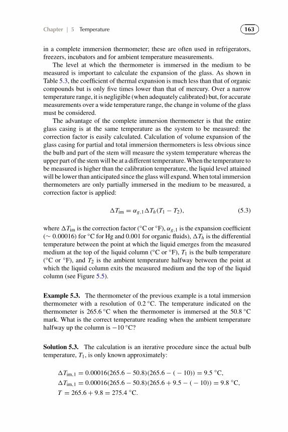
163Chapter | 5 Temperature
in a complete immersion thermometer; these are often used in refrigerators,freezers, incubators and for ambient temperature measurements.
The level at which the thermometer is immersed in the medium to bemeasured is important to calculate the expansion of the glass. As shown inTable 5.3, the coefficient of thermal expansion is much less than that of organiccompounds but is only five times lower than that of mercury. Over a narrowtemperature range, it is negligible (when adequately calibrated) but, for accuratemeasurements over a wide temperature range, the change in volume of the glassmust be considered.
The advantage of the complete immersion thermometer is that the entireglass casing is at the same temperature as the system to be measured: thecorrection factor is easily calculated. Calculation of volume expansion of theglass casing for partial and total immersion thermometers is less obvious sincethe bulb and part of the stem will measure the system temperature whereas theupper part of the stem will be at a different temperature. When the temperature tobe measured is higher than the calibration temperature, the liquid level attainedwill be lower than anticipated since the glass will expand. When total immersionthermometers are only partially immersed in the medium to be measured, acorrection factor is applied:
�Tim = αg,1�Th(T1 − T2), (5.3)
where �Tim is the correction factor (◦C or ◦F), αg,1 is the expansion coefficient(∼ 0.00016) for ◦C for Hg and 0.001 for organic fluids), �Th is the differentialtemperature between the point at which the liquid emerges from the measuredmedium at the top of the liquid column (◦C or ◦F), T1 is the bulb temperature(◦C or ◦F), and T2 is the ambient temperature halfway between the point atwhich the liquid column exits the measured medium and the top of the liquidcolumn (see Figure 5.5).
Example 5.3. The thermometer of the previous example is a total immersionthermometer with a resolution of 0.2 ◦C. The temperature indicated on thethermometer is 265.6 ◦C when the thermometer is immersed at the 50.8 ◦Cmark. What is the correct temperature reading when the ambient temperaturehalfway up the column is −10 ◦C?
Solution 5.3. The calculation is an iterative procedure since the actual bulbtemperature, T1, is only known approximately:
�Tim,1 = 0.00016(265.6 − 50.8)(265.6 − ( − 10)) = 9.5 ◦C,
�Tim,1 = 0.00016(265.6 − 50.8)(265.6 + 9.5 − ( − 10)) = 9.8 ◦C,
T = 265.6 + 9.8 = 275.4 ◦C.

164 Experimental Methods and Instrumentation for Chemical Engineers
T2
T1
ΔTh
ΔTh1/2
FIGURE 5.5 Thermocouple Immersion
5.3.3 Bimetallic Thermometers
Gas volume (or pressure) increases proportionately with temperature. Thevolume of organic liquids, aqueous solutions, mercury and eutectic alloysincreases linearly over a narrow range of temperatures but their coefficientof expansion is several orders of magnitude lower than for gases. Thermalexpansion coefficients of metals are even lower—three orders of magnitudelower than for liquids (Table 5.4). However, when two metals are bondedtogether, the difference in their thermal expansion coefficients causes the strip tocurve. When the strip is heated beyond the temperature that they were weldedtogether, the strip will bend away from the metal with the highest thermalexpansion coefficient. When it is cooled, the curvature will be toward the metalwith the highest heat transfer coefficient.
The strips may be bands or even coils. Coils are more sensitive tochanges in temperature. Although they may operate up to temperatures ashigh as 1000 ◦C, they are more typically used as thermostats for applicationsnear ambient temperature and in typical household appliances includingrefrigerators, freezers, irons, and hair and clothes dryers.
Thermostats may be used to indicate temperature but their main applicationis in the regulation of heating and cooling and as circuit breakers. They aremuch less sensitive than liquid-in-glass thermometers and achieving accuracybelow 0.1 ◦C is unrealistic. The strip is fixed at one end which is attached toan electrical power supply. The other end is free to move up and down. Forheating applications, the dial sets the position in which the free end completesan electrical circuit, which will then heat the strip. When the strip temperaturerises beyond the set-point (the desired temperature set by the manual dial), theband will move in the opposite direction, thus breaking the contact. At this

165Chapter | 5 Temperature�
�
�
�
TABLE 5.4 Mechanical and Thermal Properties of Metals Used inBimetallic Strips
Metal Therm. Exp. Coeff. Modulus of Elast.×106 K,α GPa, E
316 Stainless Steel 15.3 214
Zinc 31.0 69.4
Chromium 6.5 279
Copper 17.0 138
Tin 23.5 58.2
Aluminium 23.5 75.2
Brass 20.2 96.5
Invar (Fe/Ni—64:36) 1.7 147
Nickel 13.3 177
Monel 400 13.5 179
Inconel 702 12.5 217
Rivet Contact
Bimetallic Strip
Dial
Wire
Heating
FIGURE 5.6 Thermostat Configuration with a Bimetallic Strip
point, the band will begin to cool and move back toward the contact point tocomplete the circuit. Figure 5.6 demonstrates the curvature of the band togetherwith a typical configuration for a heating application.
The radius of curvature depends on the physical properties of the bondedmetals, their thicknesses, as well as the temperature at which they were welded:
r = t[3(1 + m)2 + (1 + mn)(m2 + 1/mn)]6(α2 − α1)(T − To)(1 + m)2 , (5.4)
where r is the radius of curvature, t is the sum of the thickness of each strip, α1is the coefficient of expansion of the metal with the lowest coefficient, α2 is thecoefficient of expansion of the metal with the highest coefficient, m is the ratioof the thickness t1/t2 where t1 corresponds to α1 (m � 1), G1 is the Young’smodulus of the metal with the lowest modulus, G2 is the Young’s modulus of
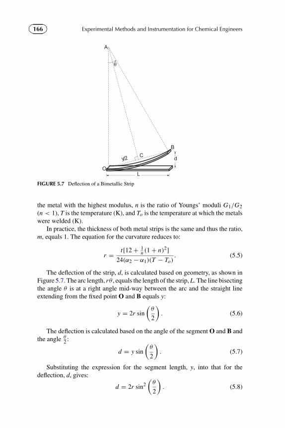
166 Experimental Methods and Instrumentation for Chemical Engineers
y/2
L
dC
O
A
B
θ
FIGURE 5.7 Deflection of a Bimetallic Strip
the metal with the highest modulus, n is the ratio of Youngs’ moduli G1/G2(n < 1), T is the temperature (K), and To is the temperature at which the metalswere welded (K).
In practice, the thickness of both metal strips is the same and thus the ratio,m, equals 1. The equation for the curvature reduces to:
r = t[12 + 1n (1 + n)2]
24(α2 − α1)(T − To). (5.5)
The deflection of the strip, d, is calculated based on geometry, as shown inFigure 5.7. The arc length, rθ , equals the length of the strip, L. The line bisectingthe angle θ is at a right angle mid-way between the arc and the straight lineextending from the fixed point O and B equals y:
y = 2r sin
(θ
2
). (5.6)
The deflection is calculated based on the angle of the segment O and B andthe angle θ
2 :
d = y sin
(θ
2
). (5.7)
Substituting the expression for the segment length, y, into that for thedeflection, d, gives:
d = 2r sin2(
θ
2
). (5.8)

167Chapter | 5 Temperature
At low levels of deflection, typical of thermostats, sin(
θ2
)is approximately
equal to(
θ2
), so the expression for deflection may be simplified to:
d = 2r sin2(
θ
2
)= 2r
(θ
2
)2
= 2r
(L
2r
)2
= L2
2r. (5.9)
Example 5.4. Brass and Inconel strips 10.0 cm long are welded together at50 ◦C. The thickness of each strip is 0.30 mm. Calculate the radius of curvaturetogether with the deflection when the strip is heated to 150 ◦C.
Solution 5.4. The physical properties for the metals are given in Table 5.4:
n = 96.5/217 = 0.445,
α2 = 2.02 × 10⁻⁵ K−1,
α1 = 1.25 × 10⁻⁵ K−1,
m = 0.30 mm/0.30 mm = 1.0,
t = 0.30 + 0.30 mm = 0.60 mm,
T = 150 ◦C,
To = 50 ◦C.
Since the thickness of each strip is equal, the simplified form to calculate thecurvature is applicable:
r = t[12 + 1n (1 + n)2]
24(α2 − α1)(T − To),
r = 0.60[12 + 10.445 1.4452]
24(2.02 × 10⁻⁵ − 1.25 × 10⁻⁵)(150 − 50.)= 542 mm ≈ 0.54 m.
The simplified expression to calculate the deflection gives:
d = L2
2r= 1002
2 · 542= 9.2 mm.
To verify, we calculate the complete expression for the deflection: the radius ofcurvature of the 100 mm strip is 542 mm and so the angle from the fixed pointto the other end is:
θ = L/r = 0.1/0.542 = 0.185,
and thus
d = 2r sin2(
θ
2
)= 2 · 542 · sin2 0.185/2 = 9.2 mm.
The simplified expression is an excellent approximation for the deflection atlow angles, which is the case for most flat bimetallic strips.
168 Experimental Methods and Instrumentation for Chemical Engineers
5.4 ELECTRICAL INSTRUMENTS
Electrical instrumentation, including thermistors and resistance temperaturedetectors (RTDs), is virtually the only type of instrumentation used inchemical processes for monitoring and control due to their versatility, accuracy,repeatability, and rapid response time. Each relies on an electrical signal, whichmay then be amplified, compensated (for calibration) and filtered before a signalis relayed either to a database or displayed. Thermistors rely on the change ofelectrical resistance with temperature of semi-conductors whereas RTDs arefabricated from pure metals. Thermocouples are the most widely used deviceand they are based on measuring the change in electrical potential (emf) withtemperature: when two dissimilar metals come into contact, emf is generatedand this emf varies with temperature.
5.4.1 Thermistors
Common thermistors are based on semiconductors whose resistancedecreases significantly as the temperature increases. Currently, thermistorsare manufactured from many different materials including polymers andother ceramics and their resistance may either increase with temperature(positive temperature coefficient—PTC) or decrease with temperature (negativetemperature coefficient—NTC). The conductivity of pure metals increases withincreasing temperatures and instruments based on metals are referred to asRTDs.
Because of their the sensitivity to temperature, thermistors made with semi-conductors are among those with the highest precision of any of the electricaltransducers with a resolution as good as 0.01 ◦C. Together with the highsensitivity, thermistors are inexpensive to manufacture and are compact. Onesubstantial limitation is that they only work over a narrow temperature range,which is typically lower than 150 ◦C and higher than −80 ◦C.
Over a very narrow range of temperatures, the resistance, R, varies linearlywith temperature:
�R = k�T , (5.10)
but to calculate the temperature accurately, a third-order nonlinear polynomialexpression is necessary—the Steinhart-Hart equation:
1
T= a + b ln R + c ln3 R, (5.11)
where a,b, and c are constants specific to each thermistor. The constant a maybe eliminated from the equation but measuring the resistance, Ro, at a knownreference temperature To, to give:
1
T= 1
To+ b ln R/Ro + c ln3 R/Ro. (5.12)

169Chapter | 5 Temperature
The value of c is often negligible for NTC resistors, thus the variation ofresistance as a function of temperature may be written as:
R = Roeβ(1/T −1/To), (5.13)
where the factor β typically varies from 3500 K to 4600 K.
Example 5.5. The factor β has a value of 1420 K and its resistance equals785 ± 4 � at 100 ◦F.
(a) What would the temperature reading be for a measured resistance of2315� ± 6�.
(b) Estimate the uncertainty in the temperature.(c) If the uncertainty in the reference temperature were 0.2, what would be the
uncertainty in temperature?
Solution 5.5a. The first step is to convert ◦F into K:
To = (100 ◦F − 32 ◦F)/(1.8 ◦C) + 273.15 K = 310.9 K.
The next step is to express the temperature as a function of resistance:
R = Ro exp
(β
(1
T− 1
To
)),
1/T = 1/To + 1/β lnR
Ro.
Substituting the values of To,Ro(311 K) = 785� and R(T ) = 2315� into theequation gives:
1/T = 1/310.9 + 1/1420 ln 2315/785 = 0.00398,
T = 251.4 K = −21.8 ◦C.
Solution 5.5b. From Chapter 2, the uncertainty of a quantity is a sum of thesquares of the uncertainties of each of factor:
�2f =
(∂ f
∂x1�1
)2
+(
∂ f
∂x2�2
)2
+(
∂ f
∂x3�3
)2
+ · · · +(
∂ f
∂xn�n
)2
.
For the case of exponential functions, f = xa11 xa2
2 xa33 xa4
4 . . . xann , a simple
expression was derived that gives:
� f
f=
√√√√ n∑i=1
(ai
xi�i )2.
170 Experimental Methods and Instrumentation for Chemical Engineers
However, in this case, the functional relationship involves a logarithm andtherefore, the partial derivatives with respect to each of the factors must bederived as given below:
∂T
∂ R= − β/R
[ln R/Ro + β/To]2 = − 1420/2315
[ln 2315/785 + 1420/311]2 = 0.0192,
∂T
∂ Ro= − β/Ro
[ln R/Ro + β/To]2 = − 1420/785
[ln 2315/785 + 1420/311]2 = 0.0567.
The uncertainty in the resistance at the reference temperature, �Ro , and themeasured temperature, �R , was 4� and 6�, respectively:
�T =√(
∂T
∂ R�R
)2
+(
∂T
∂ Ro�Ro
)2
.
5.4.2 Resistance Temperature Devices (RTDs)
As with thermistors, in order to record a signal, a DC current must be appliedacross the filament to generate a voltage from which the resistance is thenderived:
R = V /I . (5.14)
RTDs are manufactured with pure metals as opposed to semi-conductors(for thermistors) and their resistance increases with temperature, which makesthem among the most expensive instruments to measure temperature.
Over most temperature ranges the variation is linear:
αT = R − Ro
Ro(T − To)= 1
Ro
d R
dT, (5.15)
where αT is the temperature coefficient of resistance (K −1),Ro is the referenceresistance (�), and To is the reference temperature (K or ◦C).
The resistance is expressed as a function of temperature and the standardconditions by:
R = Ro[αT (T − To) + 1]. (5.16)
Platinum wire is the metal of choice because of its linearity, its chemicalinertness, and its accuracy, which increases with purity. Other metals are alsoused and their characteristics are given in Table 5.5. Temperature ranges for PtRTDs range from −260 ◦C to 660 ◦C, which is significantly greater than forthermistors. Temperatures as high as 850 ◦C are also possible but it is difficultto avoid contamination of the platinum by the thermometer metal sheath.
Commercial thermistors are manufacture to certain standards, the mostcommon of which is the Pt100—a platinum metal element with a standardresistance of 100 � (Ro) at a standard temperature of 0 ◦C (To).

171Chapter | 5 Temperature�
�
�
�
TABLE 5.5 Resistance Properties of Selected Metals Used in RTDsTo = 20◦C (Haynes, 1996)
Metal αT (K−1) R (µ� cm)
Ni 0.0067 6.85
W 0.0048 5.65
Al 0.0045 2.65
Cu 0.0043 1.67
Pb 0.0042 20.6
Ag 0.0041 1.59
Au 0.004 2.35
Pt 0.00385 10.5
Semiconductor −0.068 to 0.14 109
For a very large temperature range, the resistance no longer varies linearlywith temperature and a quadratic expression becomes necessary:
R = Ro(1 + aT + bT 2). (5.17)
In addition to the nonlinearity of the resistance with respect to temperature,another critical factor that may introduce error in the measurement is due tothe heating caused by the electrical current required to generate the signal. Thepower (heat) generated, qE , by an electrical current through a wire is related tothe resistance and current:
qE = I 2 R = I V = V 2/R. (5.18)
The change in temperature induced by the current is related to the powerproduced and the rate of energy dissipated to the surroundings (qdiss), which isrepresented by a coefficient KT :
qdiss = KT (TR − T ), (5.19)
where TR is the temperature of the thermistor and T is the ambient temperature(quantity of interest).
Solving for the temperature as a function of resistance gives the temperaturedifference between the ambient conditions and the thermistor:
T = TR − 1
KT
V 2
R. (5.20)
The dissipation coefficient, KT , is on the order of 1.5 m W K−1 in still air.Values double that are realistic in flowing situations. The temperature of the

172 Experimental Methods and Instrumentation for Chemical Engineers
thermistor, TR , is calculated based on either the linear or quadratic expressionfor resistance as a function of temperature to calculate:
TR = To − 1
αT(R/Ro − 1). (5.21)
Example 5.6. Calculate the temperature of gas estimated by a Pt100 thermistorfor which the resistance equals 200 � when a voltage of 40 mV is applied. Whatis the temperature difference between the thermistor and the gas?
Solution 5.6. For a Pt100 thermistor, the resistance, Ro, is 100 � at atemperature of 0◦C(To). The temperature coefficient of resistance, αT , for Ptequals 0.00385 K. In stagnant air, we assume that the dissipation coefficient,KT , equals 1.5 m W k−1. The temperature of the resistor, assuming a linearrelationship, is:
TR = To − 1
αT(R/Ro − 1) = 0 − 1
0.00385(100/200 − 1) = 129.9 ◦C.
The temperature of air is calculated from:
T = TR − 1
KT
V 2
R= 129.9 − 1
1.5
402
200= 124.6 ◦C = 125 ◦C.
The temperature difference due to heating is simply T − TR = 5 ◦C.
5.4.3 Thermocouples
Thermocouples are the most common instrument to measure temperature inthe chemical industry. They are versatile, compact, are applicable over a widetemperature range, and are relatively inexpensive. Not only are they used asa means to monitor the process, they are used to troubleshoot, identify areasof non-uniformity, and even determine the hydrodynamic pattern of fluids inmotion. The technique of detecting flow maldistribution based on measuring theconcentration is demonstrated in Figures 2.10 and 2.11. In Figure 5.8, both theconcentration profile and temperature profile of an experimental methanationfluidized bed reactor are illustrated:
CO + 3H2 → CH4 + H2O.
The reaction is highly exothermic and to maximize performance and avoidoverheating that might destroy the catalyst, it is important to avoid hot spots.Hot spots are regions in which the local temperature rises significantly above thedesired operating temperature and can easily exceed 100 ◦C. They result whenthe heat generated by the reaction is much greater than the heat transfer rate.

173Chapter | 5 Temperature
FIGURE 5.8 Fluidized Bed Methanation: Concentration and Temperature Axial Profiles(Kopyscinski, 2009)
The CO and H2 are fed to the fluidized bed as a stoichiometric mixture (threemoles of hydrogen for every one mole of carbon monoxide). Within the first 1cm, the concentration of hydrogen drops from 60% to 10%. If the temperaturewere not measured simultaneously with the concentration, several hypothesescould adequately account for the drop—for example, one might consider thatthe mass transfer rate throughout the bed was extremely high. However, thetemperature at the entrance drops from a maximum of approximately 400 ◦Cto around 300 ◦C coincidentally with the drop in concentration.
These measurements are based on steady-state conditions. Thermocouplesare also used to measure transients and are linked to safety alarms and interlocksto avoid hazardous conditions. For example, catalyst oxides can selectivelyconvert alkanes and alkenes (paraffins and olefins) to oxygenated products.Oxygen is often co-fed to these processes and under some conditions maycombust the hydrocarbon or form an explosive mixture (Hutchenson et al.,2010). When these conditions arise, it is critical for the instrumentation todetect changes in temperature in less than a second to change to non-hazardousoperating conditions, i.e. reducing the oxygen or hydrocarbon feed rate orflooding the system with nitrogen, etc. Thermocouples are used for theseconditions not only because of their rapid response times but also becausethey may be easily adapted to different geometries as well as being robust.
In 1821, T.J. Seebeck discovered that when two distinct metals were joinedat a point as part of a circuit at different temperatures, a compass needle couldbe deflected. Later he determined that the temperature difference caused anelectrical current and the voltage generated was close to proportional to the�T . An example of a circuit is shown in Figure 5.9, where Th is referred toas the hot junction and Tc represents the cold junction and A and B representtwo dissimilar metals (or alloys). The voltage resulting from joining two metals

174 Experimental Methods and Instrumentation for Chemical Engineers
Cu
BA
Tc
ATh
Junction 1
Junction 2
Ice Water
Potentiometer
•
•
••
B Cu
FIGURE 5.9 Thermocouple Configuration
at different temperatures is referred to as the Seebeck effect (although it wasNobili in 1829 who invented the first thermocouple).
Peltier showed in 1834 that by passing a current through two dissimilarmetals, the junction would heat up in one direction and cool down in the oppositedirection. This is known as the Peltier effect and can be used to liqueify nitrogen(−196 ◦C).
Over a narrow range of temperatures, the electromotive force (�E or emf)is directly proportional to the temperature differential (�T ):
�E = αs�T , (5.22)
where αs is the Seebeck coefficient (µV K−1).The Seebeck coefficient varies with the metal pair and many combinations
are used. Table 5.6 lists common metal pairs together with their temperaturerange and corresponding voltage and the Seebeck coefficient. The most commonthermocouples are the Types J and K. The Type J thermocouple is composed ofiron and constantan, which is a copper-nickel alloy. It has a wide temperaturerange from −210 ◦C to 760 ◦C and the second highest Seebeck coefficientof 50.2µ VK−1, resulting in a higher degree of precision. The Type Kthermocouple is made of two alloys—chromel (nickel and chromium) andalumel (nickel, manganese, and aluminum). Its Seebeck coefficient is lowerbut it can be used at temperatures as high as 1372 ◦C. A Type C thermocouplemeasures temperatures almost 1000 ◦C higher than that of a Type K and containstungsten and rhenium.
To achieve a better accuracy over a large temperature range, the emf iscorrelated to a third-order polynomial with respect to temperature:
E = AT + BT 2/2 + CT 3/3. (5.23)
Alternatively, the emf may be read from NIST thermocouple reference tablesthat list the voltages as a function of temperature differential in 1 ◦C increments

175Chapter | 5 Temperature�
�
�
�
TABLE 5.6 Principal Thermocouple Types, Compositions, and OperatingRange (Holman, 2001)
Temp. Emf Seebeck Coeff.Type Composition, Polarity (◦C) (mV) (µV K−1) T (◦C)
T ( + ) Copper −270 to 400 −6.258 to 20.872 38 0
( − ) Constantan [55% Cu, 45% Ni]
J ( + ) Iron −210 to 760 −8.095 to 42.919 50.2 0
( − ) Constantan [55% Cu, 45% Ni]
K ( + ) Chromel [90% Ni, 10% Cr] −270–1372 −6.458 to 54.886 39.4 0
( − ) Alumel [94% Ni, 3% Mn, 2% Al,1% Si]
E ( + ) Chromel [90% Ni, 10% Cr] −270 to 1000 −9.835 to 76.373 58.8 0
( − ) Constantan [55% Cu, 45% Ni]
S (+) Platinum—10% Rhodium −50 to 1768 −0.2356 to 18.693 10.3 600
( − ) Platinum
R ( + ) Platinum—13% Rhodium −50 to 1768 −0.226 to 21.101 11.5 600
( − ) Platinum
C ( + ) Tungsten—5% Rhenium 0–2320 0–33.0 19.5 600
( − ) Tungsten—26% Rhenium
(Burns et al., 1993). The voltages for Type J, K, and T thermocouples aregiven in Tables 5.7–5.9, respectively, at 10 ◦C increments (Burns et al., 1993).Note that since 0 ◦C is selected as the reference temperature, the temperaturedifferential is simply equal to the temperature. Standardizing the voltage to 0 ◦Cas a reference point (cold junction) has an advantage with respect to simplicityin reporting temperature but also experimentally: it is the most reproducibletemperature.
The choice of thermocouple type is generally related to the temperatureand the “bare wire environment” but accuracy can also be an importantconsideration; it depends on the chosen metals (or alloy) but the geometry of theapplication is also a factor. Besides the Seebeck and Peltier effects a third effectthat might need consideration is the Thomson effect: a potential could be createddue to a temperature gradient along the length of the thermocouple wires.
Together with these effects, multiple grades of thermocouples for each typeare available. For Type J thermocouples, the error of the standard grade is 2.2 ◦C(or 0.75%, whichever is greater); the error of the special grade is 1.1 ◦C (or 0.4%,whichever is greater). The Type K thermocouple has the same error (for bothgrades) above 0 ◦C but below 0 ◦C, the error is 2.2 ◦C or 2.0% for the standardgrade. The Type T thermocouple has a slightly lower error limit at 1.0 ◦C and0.75% above 0 ◦C and 1.0 ◦C and 1.5% below zero. The special grade has anerror of only 0.5 ◦C or 0.4%.
Example 5.7. The potential of a thermometer is approximated by the followingthird-order polynomial.
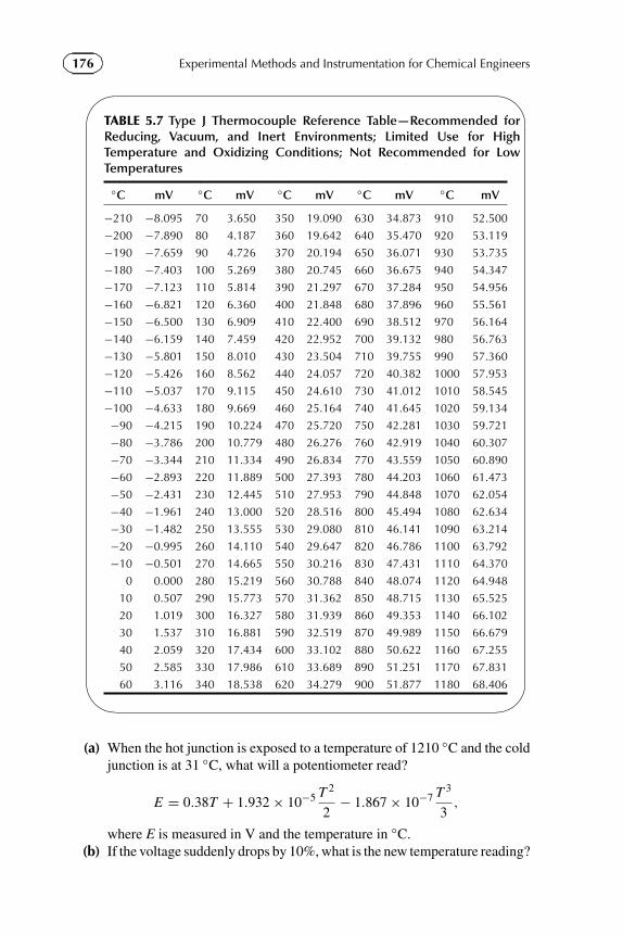
176 Experimental Methods and Instrumentation for Chemical Engineers�
�
�
�
TABLE 5.7 Type J Thermocouple Reference Table—Recommended forReducing, Vacuum, and Inert Environments; Limited Use for HighTemperature and Oxidizing Conditions; Not Recommended for LowTemperatures
◦C mV ◦C mV ◦C mV ◦C mV ◦C mV
−210 −8.095 70 3.650 350 19.090 630 34.873 910 52.500
−200 −7.890 80 4.187 360 19.642 640 35.470 920 53.119
−190 −7.659 90 4.726 370 20.194 650 36.071 930 53.735
−180 −7.403 100 5.269 380 20.745 660 36.675 940 54.347
−170 −7.123 110 5.814 390 21.297 670 37.284 950 54.956
−160 −6.821 120 6.360 400 21.848 680 37.896 960 55.561
−150 −6.500 130 6.909 410 22.400 690 38.512 970 56.164
−140 −6.159 140 7.459 420 22.952 700 39.132 980 56.763
−130 −5.801 150 8.010 430 23.504 710 39.755 990 57.360
−120 −5.426 160 8.562 440 24.057 720 40.382 1000 57.953
−110 −5.037 170 9.115 450 24.610 730 41.012 1010 58.545
−100 −4.633 180 9.669 460 25.164 740 41.645 1020 59.134
−90 −4.215 190 10.224 470 25.720 750 42.281 1030 59.721
−80 −3.786 200 10.779 480 26.276 760 42.919 1040 60.307
−70 −3.344 210 11.334 490 26.834 770 43.559 1050 60.890
−60 −2.893 220 11.889 500 27.393 780 44.203 1060 61.473
−50 −2.431 230 12.445 510 27.953 790 44.848 1070 62.054
−40 −1.961 240 13.000 520 28.516 800 45.494 1080 62.634
−30 −1.482 250 13.555 530 29.080 810 46.141 1090 63.214
−20 −0.995 260 14.110 540 29.647 820 46.786 1100 63.792
−10 −0.501 270 14.665 550 30.216 830 47.431 1110 64.370
0 0.000 280 15.219 560 30.788 840 48.074 1120 64.948
10 0.507 290 15.773 570 31.362 850 48.715 1130 65.525
20 1.019 300 16.327 580 31.939 860 49.353 1140 66.102
30 1.537 310 16.881 590 32.519 870 49.989 1150 66.679
40 2.059 320 17.434 600 33.102 880 50.622 1160 67.255
50 2.585 330 17.986 610 33.689 890 51.251 1170 67.831
60 3.116 340 18.538 620 34.279 900 51.877 1180 68.406
(a) When the hot junction is exposed to a temperature of 1210 ◦C and the coldjunction is at 31 ◦C, what will a potentiometer read?
E = 0.38T + 1.932 × 10⁻⁵ T 2
2− 1.867 × 10⁻⁷ T 3
3,
where E is measured in V and the temperature in ◦C.(b) If the voltage suddenly drops by 10%, what is the new temperature reading?

177Chapter | 5 Temperature�
�
�
�
TABLE 5.8 Type K Thermocouple Reference Table—Recommended forClean Oxidizing and Inert Environments; Limited Use for Vacuum orReducing Conditions; Wide Temperature Range
◦C mV ◦C mV ◦C mV ◦C mV ◦C mV
−270 −6.458 60 2.436 390 15.975 720 29.965 1050 43.211
−260 −6.441 70 2.851 400 16.397 730 30.382 1060 43.595
−250 −6.404 80 3.267 410 16.820 740 30.798 1070 43.978
−240 −6.344 90 3.682 420 17.243 750 31.213 1080 44.359
−230 −6.262 100 4.096 430 17.667 760 31.628 1090 44.740
−220 −6.158 110 4.509 440 18.091 770 32.041 1100 45.119
−210 −6.035 120 4.920 450 18.516 780 32.453 1110 45.497
−200 −5.891 130 5.328 460 18.941 790 32.865 1120 45.873
−190 −5.730 140 5.735 470 19.366 800 33.275 1130 46.249
−180 −5.550 150 6.138 480 19.792 810 33.685 1140 46.623
−170 −5.354 160 6.540 490 20.218 820 34.093 1150 46.995
−160 −5.141 170 6.941 500 20.644 830 34.501 1160 47.367
−150 −4.913 180 7.340 510 21.071 840 34.908 1170 47.737
−140 −4.669 190 7.739 520 21.497 850 35.313 1180 48.105
−130 −4.411 200 8.138 530 21.924 860 35.718 1190 48.473
−120 −4.138 210 8.539 540 22.350 870 36.121 1200 48.838
−110 −3.852 220 8.940 550 22.776 880 36.524 1210 49.202
−100 −3.554 230 9.343 560 23.203 890 36.925 1220 49.565
−90 −3.243 240 9.747 570 23.629 900 37.326 1230 49.926
−80 −2.920 250 10.153 580 24.055 910 37.725 1240 50.286
−70 −2.587 260 10.561 590 24.480 920 38.124 1250 50.644
−60 −2.243 270 10.971 600 24.905 930 38.522 1260 51.000
−50 −1.889 280 11.382 610 25.330 940 38.918 1270 51.355
−40 −1.527 290 11.795 620 25.755 950 39.314 1280 51.708
−30 −1.156 300 12.209 630 26.179 960 39.708 1290 52.060
−20 −0.778 310 12.624 640 26.602 970 40.101 1300 52.410
−10 −0.392 320 13.040 650 27.025 980 40.494 1310 52.759
0 0.000 330 13.457 660 27.447 990 40.885 1320 53.106
10 0.397 340 13.874 670 27.869 1000 41.276 1330 53.451
20 0.798 350 14.293 680 28.289 1010 41.665 1340 53.795
30 1.203 360 14.713 690 28.710 1020 42.053 1350 54.138
40 1.612 370 15.133 700 29.129 1030 42.440 1360 54.479
50 2.023 380 15.554 710 29.548 1040 42.826 1370 54.819
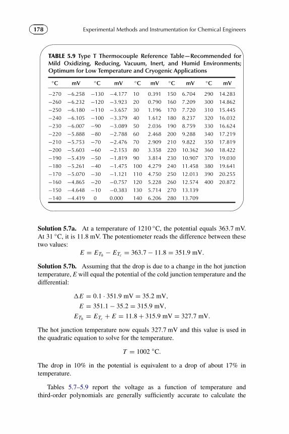
178 Experimental Methods and Instrumentation for Chemical Engineers�
�
�
�
TABLE 5.9 Type T Thermocouple Reference Table—Recommended forMild Oxidizing, Reducing, Vacuum, Inert, and Humid Environments;Optimum for Low Temperature and Cryogenic Applications
◦C mV ◦C mV ◦C mV ◦C mV ◦C mV
−270 −6.258 −130 −4.177 10 0.391 150 6.704 290 14.283
−260 −6.232 −120 −3.923 20 0.790 160 7.209 300 14.862
−250 −6.180 −110 −3.657 30 1.196 170 7.720 310 15.445
−240 −6.105 −100 −3.379 40 1.612 180 8.237 320 16.032
−230 −6.007 −90 −3.089 50 2.036 190 8.759 330 16.624
−220 −5.888 −80 −2.788 60 2.468 200 9.288 340 17.219
−210 −5.753 −70 −2.476 70 2.909 210 9.822 350 17.819
−200 −5.603 −60 −2.153 80 3.358 220 10.362 360 18.422
−190 −5.439 −50 −1.819 90 3.814 230 10.907 370 19.030
−180 −5.261 −40 −1.475 100 4.279 240 11.458 380 19.641
−170 −5.070 −30 −1.121 110 4.750 250 12.013 390 20.255
−160 −4.865 −20 −0.757 120 5.228 260 12.574 400 20.872
−150 −4.648 −10 −0.383 130 5.714 270 13.139
−140 −4.419 0 0.000 140 6.206 280 13.709
Solution 5.7a. At a temperature of 1210 ◦C, the potential equals 363.7 mV.At 31 ◦C, it is 11.8 mV. The potentiometer reads the difference between thesetwo values:
E = ETh − ETc = 363.7 − 11.8 = 351.9 mV.
Solution 5.7b. Assuming that the drop is due to a change in the hot junctiontemperature, E will equal the potential of the cold junction temperature and thedifferential:
�E = 0.1 · 351.9 mV = 35.2 mV,
E = 351.1 − 35.2 = 315.9 mV,
ETh = ETc + E = 11.8 + 315.9 mV = 327.7 mV.
The hot junction temperature now equals 327.7 mV and this value is used inthe quadratic equation to solve for the temperature.
T = 1002 ◦C.
The drop in 10% in the potential is equivalent to a drop of about 17% intemperature.
Tables 5.7–5.9 report the voltage as a function of temperature andthird-order polynomials are generally sufficiently accurate to calculate the
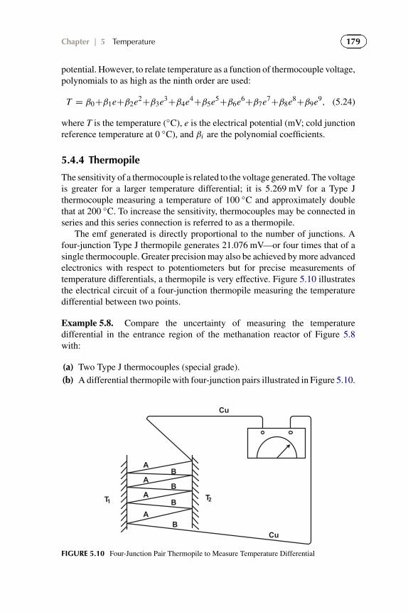
179Chapter | 5 Temperature
potential. However, to relate temperature as a function of thermocouple voltage,polynomials to as high as the ninth order are used:
T = β0+β1e+β2e2+β3e3+β4e4+β5e5+β6e6+β7e7+β8e8+β9e9, (5.24)
where T is the temperature (◦C), e is the electrical potential (mV; cold junctionreference temperature at 0 ◦C), and βi are the polynomial coefficients.
5.4.4 Thermopile
The sensitivity of a thermocouple is related to the voltage generated. The voltageis greater for a larger temperature differential; it is 5.269 mV for a Type Jthermocouple measuring a temperature of 100 ◦C and approximately doublethat at 200 ◦C. To increase the sensitivity, thermocouples may be connected inseries and this series connection is referred to as a thermopile.
The emf generated is directly proportional to the number of junctions. Afour-junction Type J thermopile generates 21.076 mV—or four times that of asingle thermocouple. Greater precision may also be achieved by more advancedelectronics with respect to potentiometers but for precise measurements oftemperature differentials, a thermopile is very effective. Figure 5.10 illustratesthe electrical circuit of a four-junction thermopile measuring the temperaturedifferential between two points.
Example 5.8. Compare the uncertainty of measuring the temperaturedifferential in the entrance region of the methanation reactor of Figure 5.8with:
(a) Two Type J thermocouples (special grade).(b) A differential thermopile with four-junction pairs illustrated in Figure 5.10.
Cu
Cu
T2T1
AB
AB
AB
AB
FIGURE 5.10 Four-Junction Pair Thermopile to Measure Temperature Differential

180 Experimental Methods and Instrumentation for Chemical Engineers
The uncertainty in the potentiometer reading is 0.1% FS for case (a) and itmeasures voltages up to 150 mV. For case (b), the full-scale reading is 15 mVwith a 0.1% error at full scale.
Solution 5.8a. The simplest approach to this problem is to calculate theuncertainty based on the square root of the sum of the squares of the twotemperature measurements. The uncertainty of the temperature reported forType J thermocouples at 400 ◦C is 1.6 ◦C (0.4% × 400 ◦C):
�T = T2 − T1,
��T = (�2T2
+ �2T1
)1/2 = (1.62 + 1.62)1/2 = 2.2 ◦C.
This approach ignores the uncertainty related to the potentiometer. To derivea more precise value, the sensitivity of the thermocouple should be taken intoconsideration either with the high-order polynomial or by deriving a lower-order polynomial in the vicinity of the temperature of interest. For a Type Jthermocouple in the range of 0–1000 ◦C, a second-order polynomial accountsfor 99.994% of the variance in the data (i.e. R2 = 0.99994):
TJ = 19.1e − 0.0328e2,
where TJ is the thermocouple temperature given in the NIST tables (Table 5.7)in ◦C and e is the voltage from Table 5.7 (mV).The error in the measured temperature, �TJ (from Chapter 2) is the partialderivative of the temperature function with respect to the voltage:
�2TJ
=(
∂TJ
∂e�e
)2
=(
∂
∂e(19.1e − 0.0328e2)�e
)2
,
�TJ = (19.1 − 0.0656e)�e.
At 400 ◦C, the emf generated is approximately 21.8 mV. The uncertainty of theinstrument is 0.1% of 150 mV, which equals ± 0.15 mV. So, the uncertainty ofa single temperature measurement will be:
�TJ = (19.1 ◦C mV−1 − 0.0656 · 21.8 ◦C mV−1)0.15 mV = 2.7 ◦C.
The uncertainty, ��T , is calculated in the same way as for the simple approachand equals
√2 · 2.7 = 3.8 ◦C, which is almost twice as high as the previously
calculated value of 2.2 ◦C.
Solution 5.8b. The second case involves a four-junction pair thermopile. Thetotal emf recorded by the potentiometer is four times greater than for a singlejunction but the temperature difference is very small—it could be as little as1 ◦C, whereas in case (a) the emf recorded was based on a temperature of 400 ◦C.The voltage read from the potentiometer, Et , is a product of the sensitivity, S,the number of junctions, n, and the temperature differential:
Et = nS�T .

181Chapter | 5 Temperature
The expression for the temperature differential becomes:
�T = Et
nS.
The sensitivity is calculated by differentiating the potential with respect totemperature:
S = d E
dT.
In the same way a polynomial expression was derived to express the temperatureas a function of voltage, a polynomial may also be formulated that approximatesthe emf as a function of temperature:
E = β1TJ − β2T 2J .
The constants for the polynomial expression are β1 = 0.05185 and β2 =6.20 × 10⁻⁶. This relationship accounts for 99.92% of the variance in the datafor a range of temperatures from 0 ◦C to 1000 ◦C. The sensitivity is then equalto:
S = d E
dTJ= 0.05185 − 12.4 × 10⁻⁶TJ ,
S400 ◦C = 0.05185 − 12.4 × 10⁻⁶(400) = 0.469 mV ◦C−1.
Again from Chapter 2, since the expression for the temperature differential is asimple product, the expression for the uncertainty:
�2�TJ
=(
∂�TJ
∂ Et�Et
)2
+(
∂�TJ
∂S�S
)2
,
is simplified to:
��T
�T= [(�Et /Et )
2 + (�S/S)2]1/2,
��T = [(�Et /nS�T )2 + (�S/S)2]1/2�T .
The uncertainty of the potentiometer �Et = 0.00115 mV = 0.015 mVand the sensitivity of the special grade thermocouple wire is 0.4% (�S/S).The equation for the uncertainty in temperature is a function of the temperaturelevel:
��T =[(
0.015 mV
4 · 0.0469
)2
+ (0.04�T )2
]1/2
= [0.08002 + (0.04�T )2]1/2.
The uncertainty in a 5 ◦C temperature differential equals 0.22 ◦C and it is aboutdouble that (0.41 ◦C) at a differential of 10 ◦C.

182 Experimental Methods and Instrumentation for Chemical Engineers
5.4.5 Radiation
The temperature measured by a thermocouple is related to several phenomenaincluding convection, conduction, humidity, and radiation. In fluid applications,stagnant regions should be avoided. Probes should be placed in areas wherethe fluid is in motion—thus increasing the convective heat transfer rate.Radiation effects are often neglected but can be significant, particularly inlaboratory applications with electrical heating and glass/quartz equipment. Inorder to minimize complications arising from radiation, it is best to purchasethermocouples that are shielded. In the case of a probe placed in flowing gas,conduction is negligible and a heat balance gives:
h A(Tg − Tp) = σεA(T 4p − T 4
w), (5.25)
where h is the heat transfer coefficient (W m−2 K−1,A is the surface area(m2),Tg is the gas temperature (K), Tp is the probe temperature (K), Tw
is the wall temperature (K), σ is the Stefan-Boltzmann constant (5.669 ×10⁻⁸ W m−2 K−4), and ε is the surface emissivity of the probe (0 < ε < 1,i.e. 1 equals a black body).
When probes are immersed in opaque solids—catalytic reactors, forexample—the solids temperature, probe temperature, and surroundingtemperature are equal—Tp = Tw. Above the bed of solids, the reading willdepend on the surrounding environment: it may remain unchanged if the vesselwall temperature is at the same temperature as the fluid (and the stream ishighly convective); if the wall is cooler than the gas, the thermocouple willirradiate heat resulting in a lower than expected temperature; in the case wherethe walls are heated electrically, the thermocouple will be hotter than the fluidtemperature. Regardless of whether or not the stream is highly convective, thetemperature reading will be determined by the surroundings!
5.5 PYROMETRY
Co-author: Paul PatienceA pyrometer is a non-contacting temperature measurement instrument that isusually used for temperatures above 500 ◦C, although with some modificationsit can measure temperatures below room temperature. The word pyrometrycomes from the Greek words pyro (fire) and meter (measure). The basic principlerelies on the notion that all bodies emit thermal radiation proportional to theirtemperature. Pyrometers detect this thermal radiation and through Planck’s lawthe temperature can be determined.
5.5.1 Thermal Radiation
Thermal radiation is essentially a conversion of thermal energy intoelectromagnetic energy. All bodies at a temperature above absolute zero radiate

183Chapter | 5 Temperature
thermal energy. However, they can also absorb, reflect, and transmit energyfrom other sources. Absorptivity (α), reflectivity (ρ), and transmissivity (τ )
are related through the following equation:
α + ρ + τ = 1. (5.26)
Gases approach ideal transmissivity, highly polished surfaces approachideal reflectivity, and a small opening in a large hollow body approachesideal absorptivity. An ideal absorber is called a black body, as opposed to agray or non-gray body. Black bodies are perfect absorbers: they absorb allincoming energy. This makes them perfect emitters as well, because at constanttemperature, a body emits the same amount of energy it absorbs; otherwise thetemperature would either rise or drop. Kirchhoff’s law states that the absorptivityof an object is equal to its emissivity (ε), or:
ε = α. (5.27)
Planck’s distribution law relates the energy emitted by a black body to theabsolute temperature and the wavelength of the radiation:
Eλ,b = C1λ−5
exp (C2/λT ) − 1, (5.28)
where Eλ,b is the energy emitted by a black body at wavelength λ(W m−2),Tis the temperature (K), λ is the wavelength (µm), C1 is 374.18 MW µm4 m−2,and C2 is 14 388 µm K.
As temperature increases, the amount of energy emitted increases, and thepeak radiation wavelength (the wavelength at which the radiation is the highest)decreases.
Non-black bodies emit less energy than black bodies since they are notperfect absorbers (they reflect and transmit incoming radiation as well as absorbit). Non-black bodies include gray bodies and non-gray bodies. Gray bodies havea constant emissivity with respect to wavelength, while the emissivity of non-gray bodies varies with wavelength. Planck’s law can be adapted for non-idealbodies by multiplying the emissivity by the black body equation:
Eλ = ε(λ)C1λ−5
exp (C2/λT ) − 1, (5.29)
where ε(λ) is the emissivity.
5.5.2 Pyrometers
Pyrometers, also known as radiation thermometers (since they measuretemperature through radiation), essentially consist of an optical system anda detector. The optical system detects energy given off by a body and focuses

184 Experimental Methods and Instrumentation for Chemical Engineers
it onto the detector. The detector returns a value proportional to the energyradiated and is used to determine the object’s temperature.
Radiation thermometers are non-contact instruments—they can be used at adistance from the object being measured. This is useful in situations where othermethods of temperature measurement are difficult or impossible to use. Theyare classified based on the wavelength measured. Broadband pyrometers absorbenergy over a very broad range of wavelengths, while narrowband pyrometersonly absorb energy over a single wavelength. Ratio pyrometers measure radiatedenergy at two wavelengths and compare them to determine the temperature.Optical pyrometers, also known as disappearing filament pyrometers, comparethe object’s color to that of a heated filament inside the pyrometer.
Broadband pyrometers can measure thermal radiation from 0.3 µm to20 µm, depending on the instrument. No filters are used to narrow the rangeof wavelengths detected, unlike other pyrometers. In the case of broadbandpyrometers, the Stefan-Boltzmann law is used to calculate the temperature:
q = εσ T 4, (5.30)
where q is the radiant heat flux emitted by source (W m−2), ε is the emissivityof the source, σ is the Stefan-Boltzmann constant (which equals 5.6074 ×10⁻⁸ W m−2 K−4), and T is the temperature (K).
It is important that the path to the object be free of particles such asdust, gases, vapor, smoke, etc., since these obstructions will cause error in thepyrometer’s reading—these particles might absorb some of the body’s radiation,causing the pyrometer to read a lower temperature than is correct.
Narrowband pyrometers operate at a single wavelength. This isaccomplished through the use of filters. The choice of wavelength depends onthe temperature range required. Since peak radiation is achieved at decreasingwavelengths with increasing temperature, a narrowband pyrometer measuringtemperature over a shorter wavelength will tend to be used for highertemperatures. These radiation thermometers are generally used at above 500 ◦C,with a wavelength ranging from 0.65 µm to 0.85 µm.
Ratio pyrometers are a variation of narrowband pyrometers used to reducethe influence of the emissivity of the object being measured (they are especiallyuseful in cases where the emissivity varies with time). The intensity of radiationis measured at two wavelengths (λ1 and λ2) and Planck’s law is used:
Eλ1
Eλ2
=(
λ1
λ2
)5 eC2/λ2T − 1
eC2/λ1T − 1. (5.31)
If the emissivity varies little with time and the two wavelengths are close, itwill cancel out and thus not affect the result.
Disappearing filament pyrometers were among the first pyrometers used.The original optical pyrometers used red filters to limit the wavelength around0.65 µm. A tungsten filament is located inside the pyrometer and will initially

185Chapter | 5 Temperature
appear hot or cold compared to the source (the operator looks into the eyepieceto compare the filament and the source). A current is run through the filamentto adjust its temperature, and therefore its color. This current is changed untilthe filament “disappears” inside the source: they will both have the same color.A calibration curve relates the current sent through the tungsten filament andthe equivalent temperature of the source.
5.6 EXERCISES
5.1 Repeat the first example in Chapter 5 where the cylinder body is chargedwith 100 ml of acetone and mercury is the operating fluid in the U-tubemanometer (differential height is 14 in.). Discuss the potential sources oferror in this measurement and how to minimize them.
5.2 How did Sir Thomas Allbutt reduce the size of the clinical thermometerfrom 30 cm to 15 cm and reduce the response time from 20 min to 5 min?
5.3 A thermometer with a 0.4 mm ID capillary may be charged with eithergalinstan or toluene.
(a) Which of the two fluids will give a higher resolution?(b) A higher temperature range?(c) At 100 ◦C which fluid is higher in the column and by how much?
5.4 The temperature of water in a beaker on a hot plate is measuredby a “constant-volume” thermometer. The cylindrical body of thethermometer is 250 ml. It is connected directly to a Bourdon gauge andthe barometric pressure is 1.0 bar. One hundred grams of isopropanol isplaced in the body of the thermometer. What is the temperature of thewater if the pressure recorded on the Bourdon gauge is 10 kPa?
5.5 To prepare a dish of rice well, it must be cooked at a temperature of 90 ◦C.Room temperature is 25 ◦C and a Type T thermocouple is available.N. Ly
(a) Will the dish of rice be well prepared if the thermocouple indicatesa value of 3.814 mV?
(b) Calculate the value that the potentiometer should indicate to obtaina temperature of 90 ◦C.
5.6 A total immersion Hg thermometer with a range from −20 ◦C to 200 ◦Cis 40 cm in length. It is immersed in a boiling fluid in a beaker on a hotplate to a depth of 5 cm. If the thermometer reads 160 ◦C, what is theactual temperature?
5.7 (a) Derive an expression for the radius of curvature of a bimetallic stripwhen the thickness of each strip is equal and the Young’s moduli areapproximately the same.

186 Experimental Methods and Instrumentation for Chemical Engineers
(b) At what value of n does the error in the calculated value of the radiusof curvature exceed 5%?
5.8 In the sixth example in Chapter 5, what would be the uncertainty in thetemperature if the uncertainty in the reference temperature was 2 ◦F?
5.9 Derive an expression for the uncertainty of the resistance, R, of an RTDwith respect to reference resistance and temperature for the case that theresistance varies with the following quadratic:
R = R0(1 + aT + bT 2).
5.10 For the same conditions of the sixth example in Chapter 5, would thetemperature differential between the thermistor and air be greater withNi? How much lower would the temperature rise in the case of a flowinggas? Assume a Ni100 thermistor.
5.11 Derive a second-order polynomial expression relating the temperatureand emf for a Type K thermocouple from 0 ◦C to 1000 ◦C.
5.12 The internal temperature of a camel can vary from 34 ◦C to 42 ◦C inorder to adapt to the Sahara’s temperature changes—usually from 10 ◦Cto 50 ◦C during the summer. In the desert of southern Tunisia (TozeurCity), a camel’s temperature was studied during the day with a Type Tthermocouple. A voltmeter is used as a cold junction and its temperatureis estimated at 25 ◦C, 50 ◦C, 10 ◦C at 9 AM, 3 PM and 9 PM. The otherjunction is placed in the camel’s mouth. B. Sana
(a) If voltage drops are negligible, what is the temperature of thecamel if the voltmeter shows a voltage of 0.486 mV, 0.959 mV, and−0.355 mV at 9 AM, 3 PM, and 9 PM?
(b) What would the voltage indicated by the voltmeter be if the referencetemperature suddenly dropped from 10 to −1 ◦C overnight (at9 PM)?
(c) Assuming that the voltmeter measuring the emf has an uncertaintyof 0.003 mV and the temperature of the cold junction is set at a 1 ◦Cresolution, calculate the accuracy in measuring the temperature ofthe camel for Tref = 25 ◦C (9 PM).
5.13 Determine the emf indicated on three thermocouples of Types J, T, and K ifthe sample temperature is 290 K and the cold junction is in a refrigerator at4 ◦C. Keeping the junction in the refrigerator, what would the temperatureof a beer be if the emf indicated by the thermocouple is 0.203 mV?P. Malo-Couture
5.14 Repeat part (c) of the second example in Chapter 5 taking into accountthe thermal expansion properties of glass.
5.15 A copper-constantan thermocouple (Type T) is exposed to a temperatureof 500 ◦F. The cold junction temperature is estimated to be 50 ◦F.A. Benamer

187Chapter | 5 Temperature
(a) Calculate the electromotive force (emf) indicated by thepotentiometer.
(b) If the potentiometer indicates an emf of 3.723 mV, what temperature(in ◦C and ◦F) will the thermocouple be exposed to?
(c) If the temperature of the cold junction were to hit 5 ◦F, what would(a) be?
5.16 Determine the radius of curvature of a metallic strip thermometer’sbimetallic strip, composed of yellow brass and chrome. The two metalsare sealed at 60 ◦C and each band has a thickness of 0.20 mm. The striphas a length of 15.0 cm when exposed to a temperature of 250 ◦C. J. Tran
5.17 An expansion thermometer—with graduations of 1 ◦C—and twothermocouples—Types T and K—are used to observe the evolution oftemperature in a heated water bath. The temperature is read directlyoff the expansion thermometer. The reference temperature for the twothermocouples is 25 ◦C and the data is summarized in Table Q5.17. Notethat the thermocouples’ precision is 0.05 mV. C. Neagoe�
�
�
�
TABLE Q5.17 Thermocouple Reference Temperature
# Exp. Therm. (◦C) Type T (mV) Type K (mV)
1 21 −0.147 −0.144
2 25 0.039 0.030
3 29 0.170 0.190
4 33 0.344 0.408
5 39 0.550 0.550
6 42 0.720 0.725
7 47 0.910 0.880
8 51 1.063 1.020
(a) Calculate the calibration curves for both thermocouples.(b) Calculate the absolute and relative errors for each device.(c) Based on the temperature values and the error of each instrument,
what can you conclude?
5.18 A butcher discovers some of his beef has putrefied from what appears tobe poor temperature control in the freezer and thus decides to replace thecontroller and measuring device. The new system consists of a thermistorwith a resitance of (800 ± 4) � at 80 ◦F and β = 3400 K. Ludmilla
(a) Determine the temperature of the freezer for a resistance of (2424 ±5) �.
(b) Determine the uncertainty of the temperature.

188 Experimental Methods and Instrumentation for Chemical Engineers
REFERENCES
Adler, M. J. 1974. Albutt, Sir Thomas Clifford. Encyclopaedia Britiannica. Micropaedia 1, 251.Berna, F., Behar, A., Shahack-Gross, R., Berg, J., Boaretto, E., Gilboa, A., Shaorn, I., Shalev,
S., Shilstein, S., Yahalom-Mack, N., Zorn, J.R., Weiner, S., 2007. Sediments exposed to hightemperatures: reconstructing pyrotechnological processes in Late Bronze and Iron Age Strata atTel Dor (Israel). Journal of Archaeological Science 34, 358–373.
Bolton, H.C., 1900. Evolution of the thermometer. The Chemical Publishing Co., pp. 1592–1743.Brown, K.S., Marean, C.W., Herries, A.I.R., Jacobs, Z., Tibolo, C., Braun, D., Roberts, D.L., Meyer,
M.C., Bernatchez J., 2009. Fire as an engineering tool of early modern humans. Science 325,859–862.
Burns, G. W. , Strouse, G. F., Croarkin, M. C., Guthrie, W.F., 1993. NIST Mono. 175 ThermocoupleReference Functions on ITS–90.
Goren, Y., Goring-Morris, A.N., 2008. Early pyrotechnology in the near east: experimental lime-plaster production at the pre-pottery neolithic B site of Kfar HaHoresh, Israel. Geoarchaelogy:An International Journal 23 (6), 779–798.
Goren-Inbar, N., Alperson, N., Kislev, M.E., Simchoni, O., Melamed, Y., Ben-Nun, A., Werker, E.,2004. Evidence of hominin control of fire at gesher benot ya’aqov, Israel. Science 304 (5671),725–727.
Haynes, W.M. (Ed.), 1996. CRC Handbook of Chemistry and Physics, 92nd ed. CRC Press.Holman, J.P., 2001. Experimental Methods for Engineers, seventh ed. McGraw-Hill Inc., New
York.Hummel, R.E., 2005. Understanding Materials Science: History, Properties, Applications, second
ed. Springer.Hutchenson, K .W., LaMarca, C., Patience, G.S., Laviolette, J.-P., Bockrath, R.E., 2010. Parametric
study of Homogeneous Oxidation of Butane in a Circulating Fluidized Bed Reactor. ApplicationsCatalysis A: General 376, 91–103.
Knoblauch, M., Hibberd, J.M., Gray, J.C., van Bel, A.J.E., 1999. A galinstan expansionfemtosyringe for microinjection of eukaryotic organelles and prokaryotes. Nature Biotechnology17, 906–909.
Kopyscinski, J., Schildhauer, T.J., Biollaz, S.M.A. 2009. “Employing Catalyst Fluidization toEnable Carbon Management in the Synthetic Natural Gas Production from Biomass”, Chem.Eng. Technol., 32 (3) 343–347.
Temperature Measurement, Wiley.Nicholson, P.T., Shaw, I., 2000. Ancient Egyptian materials and Technology, Cambridge University
Press.Rothfusz, L.P., 1990. The Heat Index “Equation” (or, More Than You Ever Wanted to Know About
Heat Index), Scientific Services Division (NWS Southern Region Headquarters) SR 90–23.Sherwood-Taylor, F., 1942. The origin of the thermometer. Annals of Science 5 (2), 129–156.Steadman, R.G., 1979. The Assessment of sultriness. Part I: a temperature-humidity index based
on human physiology and clothing science. Journal of Applied Meteorology 18, 861–873.Thieme, H., 1997. Lower palaeolithic hunting spears from Germany. Nature 385, 807.Weisberger, G., Willies, L., 2001. The use of fire in prehistoric and ancient mining: firesetting.
Paleorient 26 (2), 121–149.

Chapter 6
Fluid Metering
6.1 OVERVIEW
Fluid flow is not only a critical aspect of the process industry: it had a tremendousimportance in the development of ancient civilizations. The Sumerians in4000 BC were the first to use canals for irrigation. Babylon is known to havehad toilets and Sargon II’s (700 BC) palace had drains connected to a 1 mhigh and 5 m long sewer that ran along the outer wall of the city. Sargon II’sson, Sennacherib, was the first to build an aqueduct (65 km long), which wasconstructed for the Assyrian capital city Nineveh. In the Persian AchaemenianEmpire, qanats were invented that tapped ground water and relied on gravityas the driving force for transport: underground tunnels were dug to the levelof the ground water at one point and sloped downwards toward the exit.Nebuchadnezzar is credited for erecting the Hanging Gardens of Babylon: Waterwas fed to the gardens through the use of a noria—a water wheel, which couldbe considered one of the first automatic pumps. Norias were been designed todeliver water for irrigation at rates of up to 2500 l h−1. The largest water wheelwas 20 m tall and was built in Hama, Syria. Prior to water wheels, manual pumpscalled shadoofs were used to raise water from wells in Mesopotamia (2000 BC)and from the Nile in Egypt. Maximum rates are of the order of 2500 l d−1 at amaximum height of about 3 m. In 200 BC the reciprocating pump was inventedby Ctesibius and Archimedes described the screw pump (some believe that thescrew pump was used 500 years earlier in Babylon). Bellows may be consideredthe first air pump and were used by the Egyptians in 1490 BC. In the fifth centuryBC, the Chinese developed double-action piston bellows and Du Shi of Chinaadapted a water wheel to power a bellows used for smelting iron.
Experimental Methods and Instrumentation for Chemical Engineers. http://dx.doi.org/10.1016/B978-0-444-53804-8.00006-X© 2013 Elsevier B.V. All rights reserved. 189

190 Experimental Methods and Instrumentation for Chemical Engineers
The Romans mastered hydraulic engineering, which is principallyconcerned with the transport of water and sewage. Fresh water was supplied toRome through 10 independent aqueducts that varied in length from 15 km to91 km, the first of which was built in 312 BC. Estimates of the daily flow raterange from 300 kt d−1 to 1000 kt d−1. Transporting water over these greatdistances required regulation basins, culverts, and energy dissipaters calledstepped and dropshaft cascade chutes. The design tolerances for the aqueductsdownward gradient were as low as 20 cm km−1.
Together with the aqueducts, the Romans also advanced the technologyof water distribution from the aqueducts to multiple sites—baths, residences,fountains, etc. Plumbing is derived from the Latin word plumbum which meanslead. Piping used in Roman times included lead pipes, masonry channels aswell as earthenware pipes. The water was delivered to baths and some publichomes at a constant rate. The cost of the water was charged based on the pipecross-sectional area, which served as a restriction orifice (Chanson, 2002, 2008).
Whereas the transport of water to major centers allowed civilizations toflourish, the measurement and control of fluid flow has been a critical aspect ofthe development of industrial processes. Not only is metering flow importantto maintaining stable and safe operating conditions, it is the prime means toaccount for the raw materials consumed and the finished products manufactured.While pressure and temperature are critical operating parameters for plantsafety, the measurement of flow rate has a direct impact on process economics.For basic chemicals (as opposed to specialty chemicals or pharmaceuticals) likeethylene, propylene, methanol, sulfuric acid, etc. profit margins are relativelylow and volumes are large, so high precision instruments are required to ensurethe economic viability of the process.
Flow meters are instruments that measure the quantity of movement of afluid in a duct, pipe, or open space. The fluid can be water, a liquid solution, achemical product or slurry, gas or vapor, and even solid—powders, for example.In everyday life, we use flow meters to pump gasoline into automobile fuel tanks,methane gas is metered to houses and metering water to houses is becomingmore common. With respect to anatomy, the heart’s pumping action ensuresblood circulation and lung health is assessed by measuring the volume of airthe lungs can hold. Trees are amazing for their ability to transport water inxylem and phloem for vertical distances exceeding 100 m!
Despite the importance of transporting water and its contribution to the riseof many great civilizations, most of the ancient technology used to build andmaintain aqueducts, water distribution, and sewage systems was lost. Romedeclined from a city of 1.6 million habitants at its zenith in 100 AD to lessthan 30 000 during the dark ages up until the Renaissance partly because of thedestroyed aqueducts that remained in disrepair.

191Chapter | 6 Fluid Metering
6.2 FLUID DYNAMICS
Modern fluid dynamics was pioneered by the Swiss physicist Bernoulli whopublished the book entitled “Hydrodynamica” in 1738. Bernoulli’s workis based on the principle of the conservation of energy, which holds thatmechanical energy along a streamline is constant. He demonstrated thatincreasing the potential energy of a flowing fluid (by raising the elevation ofa pipe, for example) reduces the pressure of the fluid in the pipe (above thatwhich would be expected based on wall friction); decreasing the cross-sectionof the pipe increases the velocity head and decreases the pressure head.
Consider the flow restriction of a pipe in Figure 6.1. The fluid acceleratesfrom left to right as it passes through the restriction. Based on continuity—conservation of mass—the mass flow rate, m, crossing point 1 equals that atpoint 2:
m1 = m2,
m = ρ1 X A,1u1 = ρ2 X A,2u2, (6.1)
where ρ is the fluid density (kg m−3), X A is the cross-sectional area (m2), andu is the velocity (m s−1).
For an incompressible fluid, the fluid accelerates in proportion to the ratioof the cross-sectional areas.
Bernoulli derived an equation based on an energy balance around a fluidflowing in a pipe and is expressed in a simplified form as:
�P
ρ+ 1
2�u2 + g�Z = hf , (6.2)
where hf is the head loss due to friction.In the case of Figure 6.1, besides neglecting friction losses (as well as some
other simplifying assumptions), the change in elevation is equal to zero andthus the pressure drop going from point 1 to point 2 is simply calculated based
u1 u2
P 1, T 1, ρ
ρ
1, X A1
P 2, T 2, 2, X A2
FIGURE 6.1 Fluid Flow Through a Constriction
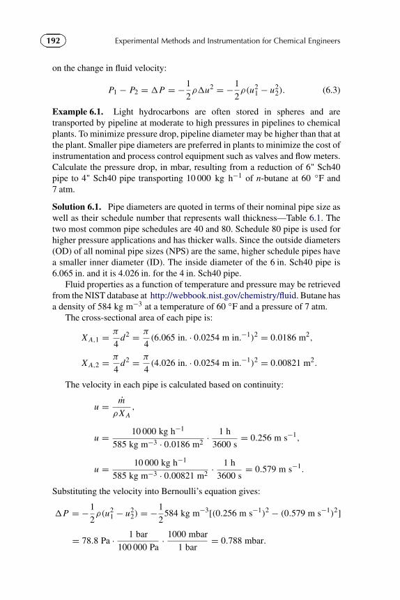
192 Experimental Methods and Instrumentation for Chemical Engineers
on the change in fluid velocity:
P1 − P2 = �P = −1
2ρ�u2 = −1
2ρ(u2
1 − u22). (6.3)
Example 6.1. Light hydrocarbons are often stored in spheres and aretransported by pipeline at moderate to high pressures in pipelines to chemicalplants. To minimize pressure drop, pipeline diameter may be higher than that atthe plant. Smaller pipe diameters are preferred in plants to minimize the cost ofinstrumentation and process control equipment such as valves and flow meters.Calculate the pressure drop, in mbar, resulting from a reduction of 6" Sch40pipe to 4" Sch40 pipe transporting 10 000 kg h−1 of n-butane at 60 ◦F and7 atm.
Solution 6.1. Pipe diameters are quoted in terms of their nominal pipe size aswell as their schedule number that represents wall thickness—Table 6.1. Thetwo most common pipe schedules are 40 and 80. Schedule 80 pipe is used forhigher pressure applications and has thicker walls. Since the outside diameters(OD) of all nominal pipe sizes (NPS) are the same, higher schedule pipes havea smaller inner diameter (ID). The inside diameter of the 6 in. Sch40 pipe is6.065 in. and it is 4.026 in. for the 4 in. Sch40 pipe.
Fluid properties as a function of temperature and pressure may be retrievedfrom the NIST database at http://webbook.nist.gov/chemistry/fluid. Butane hasa density of 584 kg m−3 at a temperature of 60 ◦F and a pressure of 7 atm.
The cross-sectional area of each pipe is:
X A,1 = π
4d2 = π
4(6.065 in. · 0.0254 m in.−1)2 = 0.0186 m2,
X A,2 = π
4d2 = π
4(4.026 in. · 0.0254 m in.−1)2 = 0.00821 m2.
The velocity in each pipe is calculated based on continuity:
u = m
ρX A,
u = 10 000 kg h−1
585 kg m−3 · 0.0186 m2 · 1 h
3600 s= 0.256 m s−1,
u = 10 000 kg h−1
585 kg m−3 · 0.00821 m2 · 1 h
3600 s= 0.579 m s−1.
Substituting the velocity into Bernoulli’s equation gives:
�P = −1
2ρ(u2
1 − u22) = −1
2584 kg m−3[(0.256 m s−1)2 − (0.579 m s−1)2]
= 78.8 Pa · 1 bar
100 000 Pa· 1000 mbar
1 bar= 0.788 mbar.

193Chapter | 6 Fluid Metering�
�
�
�
TABLE 6.1 Nominal Pipe Sizes
NPS OD (in.) Sch. No. Wall Thickness (in.) ID (in.)
1/8 0.40540 0.068 0.269
80 0.095 0.215
1/4 0.5440 0.088 0.364
80 0.119 0.302
3/8 0.67540 0.091 0.493
80 0.126 0.423
1/2 0.8440 0.109 0.622
80 0.147 0.546
1 1.31540 0.133 1.049
80 0.179 0.957
2 2.37540 0.154 2.067
80 0.218 1.939
3 3.540 0.216 3.068
80 0.300 2.900
4 4.540 0.237 4.026
80 0.337 3.826
5 5.56340 0.258 5.047
80 0.375 4.813
6 6.62540 0.280 6.065
80 0.432 5.761
8 8.62540 0.322 7.981
80 0.500 7.625
The head loss due to friction has been neglected in the calculations but it isvery important for long pipelines and in the case of elbows, valves, tees, andother restrictions. In the case of aqueduct design, restrictions were necessaryto control flow rate. In the case of pipe flow, straight lines are preferred and allobstructions and changes in direction should be minimized to minimize pressuredrop.
The pressure drop in a straight pipe is determined by factors including fluidvelocity and viscosity, pipe surface roughness as well as flow regime—whetheror not the flow is turbulent or laminar, a concept introduced by Stokes in 1851.In 1888, Osborne Reynolds conducted experiments that clearly delineated thedifference between the different flow regimes. He injected a fine filament ofcolored water in a pipe together with water. At low flow rates, the filament

194 Experimental Methods and Instrumentation for Chemical Engineers
u
FIGURE 6.2 Laminar Velocity Profile, NRe < 2000
maintained a parallel line from one end to the other. When the flow ratewas increased beyond a certain value, the colored filament would break upforming eddies and vortices. The eddies and vortices promoted mixing of thecolored water such that the filament disappeared and the color became uniformlydistributed throughout the cross-section.
At the low velocities, before the filament broke up, the velocity profile wasparabolic—the centerline velocity was twice as high as the average and the wallvelocity was essentially equal to zero, as shown in Figure 6.2.
At higher velocities the filament would form eddies and the velocity profilebecame more flat at the center—the wall velocity remained zero (Figure 6.3).
Reynolds studied the conditions at which the flow pattern transitioned fromlaminar to turbulent and derived the following relationship that is now knownas the Reynolds number, NRe:
NRe = ρu Dh
μ, (6.4)
where μ is the fluid viscosity (Pa s or kg m−1 s−1) and Dh is the hydraulicdiameter (m).
This dimensionless number is a ratio of the inertial forces, ρu Dh , to theviscous forces, μ. For circular pipes, the hydraulic diameter equals the pipediameter. For square ducts, it is equal to four times the cross-sectional areadivided by the perimeter. Subsequent experiments demonstrated that at about aReynolds number of 2000, the flow regime was no longer laminar but neither wasit entirely turbulent—this regime was designated as the intermediate regime.The turbulent regime is often considered to begin at a Reynolds number of 4000.
To calculate the Reynolds number in the previous example, all quantities areknown except for the viscosity. From the NIST (2011) database, the viscosity ofbutane at 60 ◦F and 7 atm is reported as 0.000175 Pa s. The Reynolds number
u
FIGURE 6.3 Turbulent Velocity Profile, NRe > 4000

195Chapter | 6 Fluid Metering
in the 6 in. pipe is 132 000 while it is 198 000 in the 4 in. pipe—the flow regimeis turbulent.
Non-dimensional numbers are useful to size equipment but also as scalingparameters to design experiments. Engineers use scaled models to studyphenomena that are difficult to study or prohibitively expensive: fluid flowexperiments in a 6 in. pipe or larger would require large pumps or blowers, flowmeters, valves, fittings, etc. The conditions of the experiments are chosen suchthat there is a similarity between the full-scale system and the model. Thus,the fluid, diameter, and velocities are chosen to maintain the same Reynoldsnumber.
Example 6.2. Xylem vessels are the conduits through which water istransported from the roots throughout trees and other plants up to the leaves.They have a peculiar helical geometry, as shown in Figure E6.2 and varysubstantially in diameter (and length). Design an experimental model to studythe hydrodynamics of the fluid flow using glycerol whose viscosity is 2500 cPand density equals 1250 kg m−3.
Solution 6.2. The density and viscosity of water are nominally 1000 kg m−3
and 0.001 Pa s. So, neglecting the helical inner construction and assuming acircular geometry and a linear velocity of 1 mm s−1, the Reynolds number inthe xylem is:
NRe = ρu D
μ= 1000 · 0.001 · 150 × 10−6
0.001= 0.15.
Since we have chosen to use glycerol as the model fluid because of its highviscosity and transparency, the only choice left to make is the diameter of theapparatus (which will then determine the operating velocity):
u D = μNRe
ρ= 2500 cP · 1 × 10−3 Pa s/cP · 0.15
1250 kg m−3 = 0.00030 m2 s−1.
Operating in small diameter tubes is inconvenient not only to assemblebut also because it results in high fluid velocities. With a 5 cm diameter tube
LigninCell Wall
FIGURE E6.2 Schematic of a Xylem Vessel

196 Experimental Methods and Instrumentation for Chemical Engineers
and to maintain hydrodynamic similarity, the operating fluid velocity would be6 mm s−1, which is a reasonable value to conduct visualization experiments.
6.3 FLOW METER SELECTION
Just as with the measurement of temperature and pressure, many technologieshave been invented to quantify the flow rate of gases and liquids. Crabtree(2009) identified 33 distinct technologies and divided them into eight categories.Table 6.2 includes an additional category for rotameters, which are also knownas variable area meters. The classification has lumped thermal mass flow meterstogether with Coriolis meters as “mass flow” meters. Although they do measuremass flow (as opposed to volumetric flow), the operating principles are entirelyunrelated: thermal mass flow meters measure heat transfer rates to deduce massflow while the Coriolis meter relies on the force induced by a fluid passingthrough a moving pipe that has a semicircular (or arch) shape.
The types of instruments used in an industrial setting are often differentfrom those used in the laboratory. The most common high precision laboratoryinstrument is the mass flow controller and rotameters are frequent forapplications for both gases and liquids but are much less accurate. In industry,obstruction flow meters, Coriolis meters, and vortex shedders are more standard.
Selecting a flow meter for a given application depends on several criteriaincluding:
● Process conditions.● Required precision.● Robustness.● Size.● Response time.
�
�
�
�
TABLE 6.2 Flow Meter Categories
Category Example
Positive displacement Wet test flow meters, pumps, gears, and impellers
Differential pressure Orifice, Venturi, Tuyère, Pitot tube
Variable area meter Rotameter
Mass flow Thermal mass, Coriolis
Inferential Turbine
Oscillatory Vortex
Electromagnetic Magmeters
Ultrasonic Doppler
Open channel Weir, flume

197Chapter | 6 Fluid Metering
● Resolution.● Facility of installation.● Price.● Maintenance frequency.● Operator preference (familiarity).● Repeatability.
Crabtree (2009) detailed most of the flow meters used in industrial plants.His classification for selecting measuring technology with respect to processapplication is reproduced in Table 6.3. All flow meters are suitable for cleanliquids except for the Ultrasonic-Doppler instrument and only electromagneticinstruments are unsuitable for low conductivity fluids. Most instruments aresuitable for high temperature operation or application under certain conditionsexcept for the ultrasonic instruments. Many flow meters are suitable for gases.Few instruments can be used for open channel flow or pipes that are semifilledwith the exception of weirs and flumes.
The more common flow meters are discussed in some detail further on.The following is a brief discussion of the open channel, ultrasonic, andelectromagnetic flow meters. Open channel meters are found in irrigationapplications as well as in waste water treatment, mining beneficiation, andsewage. The principle is to change the level of the water by introducing ahydraulic structure in the flow then inferring the flow rate by the change in level.
Electromagnetic flow meters (magmeters) are considered to be the idealflow meter for conductive fluids—they are unsuitable for hydrocarbons, gases,steam, or ultra-pure water. They have a high range of operability, an accuracyof ±0.1%, low space requirements, and are non-intrusive (that is, they do notaffect the flow field). The principle is based on measuring the voltage inducedwhen a conductive object passes a magnetic field. The voltage is proportionalto the velocity.
Ultrasonic meters have been available for several decades and are analternative to magmeters for measuring flow non-intrusively. They are suitablefor a large range of pipe sizes and are particularly economic versus othermethods for large diameter pipe with an accuracy of about 1%. Three typesof meters are manufactured: Doppler, transit time, and frequency difference.The Doppler-effect meter relies on measuring the change of frequency when anultrasonic beam is directed toward or away from a moving fluid. The time-of-flight meter measures the difference in time it takes an ultrasonic beam to reachone detector upstream of the beam (in the counter-current direction of flow)and another downstream of the beam (in the co-current direction). Finally, thefrequency method sends an ultrasonic pulse to each detector and after eachsuccessive pulse reception, another signal is transmitted. The difference in thefrequency of the downstream and upstream pointing beams is related to thevelocity of the fluid. These meters require as much as 25 ppm of particles or
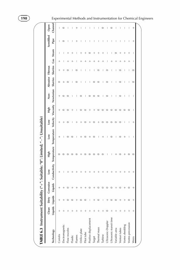
198 Experimental Methods and Instrumentation for Chemical Engineers
� �
� �
TAB
LE6.
3In
stru
men
tSu
itab
ility
(“+”
:Sui
tab
le;“
0”:L
imit
ed;“
−”:U
nsui
tab
le)
Cle
anD
irty
Co
rro
sive
Low
Hig
hLo
wLo
wH
igh
No
n-A
bra
sive
Fib
rous
Sem
ifille
dO
pen
Tech
nolo
gyLi
qui
ds
Liq
uid
sLi
qui
ds
Co
nduc
tivi
tyTe
mp
erat
ure
Tem
per
atur
eVe
loci
tyV
isco
sity
New
toni
anSl
urri
esSl
urri
esG
asSt
eam
Pip
eC
hann
el
Cor
iolis
++
++
0+
++
+0
++
−−
−El
ectr
omag
netic
++
+−
0−
+0
0+
+−
−0
0
Flow
nozz
les
+0
0+
00
00
00
0+
+−
−Fl
uidi
c+
0+
+0
0−
+−
−−
++
−−
Flum
es+
++
+0
−+
−−
00
−−
++
Ori
fice
plat
e+
0+
++
++
00
−−
++
−−
Pito
ttub
e+
0+
+0
00
0−
−−
++
−−
Posi
tive
disp
lace
men
t+
−0
+0
++
+0
−−
+0
−−
Targ
et+
++
+0
00
+0
0−
++
−−
Ther
mal
mas
s+
00
+0
−+
00
00
++
−−
Turb
ine
+−
0+
0+
00
−−
−+
+−
0
Ultr
ason
ic-D
oppl
er0
+0
+−
−0
00
00
−−
−−
Ultr
ason
ic-t
rans
ittim
e+
00
+−
00
0−
−−
+−
−0
Var
iabl
ear
ea+
0+
++
−0
0−
−−
+0
−−
Ven
turi
tube
s+
+0
+0
00
00
00
++
−−
Vor
tex
shed
ding
++
++
++
−0
−−
−+
+−
−V
orte
xpr
eces
sion
+0
0+
0−
−0
−−
−+
+−
−W
eirs
++
++
0−
+−
−0
0−
−+
+

199Chapter | 6 Fluid Metering
bubbles with a minimum 30 µm diameter: the amplitude of the Doppler signaldepends on the number of particles or discontinuities.
6.4 POSITIVE DISPLACEMENT
Positive displacement meters—direct volumetric totalizers—are often used inlaboratories for calibration. The principle is based on delivering a discretevolume of fluid in aliquots. In fact, water wheels and shadoofs could beconsidered as positive displacement meters. Pumps may also be consideredas meters.
In the medical profession, infusion pumps introduce fluids at rates as lowas 0.1 ml h−1—much lower than a drip. Peristaltic pumps force larger volumesof fluids—solutions sufficient to feed a patient—at higher rates: a roller rotatesaround a cylinder on which flexible tubing is mounted. At each rotation, theroller pinches the tube around the cylinder thereby trapping the fluid and movingit forward. Infusion pumps consist of a motor turning a screw that advances theplunger of a syringe, as shown in Figure 6.4, and can deliver aliquots of 500 nl.High pressure syringe pumps such as Isco can deliver fluids at rates of nl min−1
and pressures of 1380 bar. These types of pumps are popular for analyticalequipment such as High Performance Liquid Chromatography (HPLC).
Bubble meters are used calibrate laboratory meters that have low flow rates.The gas passes through a tee at the bottom connected to a balloon filled withsoapy water. The balloon is squeezed to force the water into the neck andthen a bubble forms as the gas passes through the liquid. The bubble ascendsin the body of the vessel and passes the graduated marks. The volumetricflow rate is determined by recording the time the bubble takes to pass twograduated marks. Remember that reference conditions to calculate the volumedisplacement correspond to the pressure and temperature of the bubble meter.
Graduated Syringe Barrel
Plunger
Plunger Block
Screw
FIGURE 6.4 Syringe Pump

200 Experimental Methods and Instrumentation for Chemical Engineers
Rubber Tube
Entrance
Exhaust DisengagementSection
Balloon with soapy water
1000 mL
800 mL
0 mL
200 mL
400 mL
600 mL
FIGURE E6.3 Bubble Flow Meter
Often meters report flow rates at standard conditions. Standard conditions mustalso be precisely defined (as mentioned in Chapter 1).
Example 6.3. The bubble flow meter, shown in Figure E6.3, consists of a1 l cylinder with graduation marks every 200 ml. The time a bubble takes tocross two graduation marks (400 ml) is recorded with a precision stopwatchwith a resolution of 0.01 s. Ten measurements are made, and the bubble meterrecording at 400 ml intervals is (in s): 4.83, 4.95, 4.78, 5.01, 5.12, 4.85, 5.09,4.70, 4.99, and 5.30.
(a) Calculate the volumetric flow rate and uncertainty assuming STP.(b) Calculate the absolute error.(c) How would the error and uncertainty change if the time was recorded
between four graduation marks instead of two?
Solution 6.3a. The mean time equals 4.96 s, which corresponds to a volumetricflow rate of 80.6 ml s−1 at ambient conditions. The volumetric flow rate atstandard conditions (sc) is calculated using the ideal gas law by convertingfrom ambient temperature and pressure (Ta and Pa , respectively):
Q = QaTa
Tsc
Psc
Pa.

201Chapter | 6 Fluid Metering
If the laboratory was operating at 1 atm and 25 ◦C, then the volumetric flowrate at STP is:
Q = Qa25 + 273.15
273.15
1
1.01325= 86.8 ml s−1 = 86.8 sccm.
The units of volumetric flow rate in the laboratory are often quoted as sccm—standard cubic centimeters per minute.
The uncertainty in the measured time, �t , is the product of the samplestandard deviation and the Student’s t-statistic for 10 sample points at a 95%confidence interval (Table 2.2):
�t = ±t(α,n − 1) · st,x = ±t(95,9)st√
n,
�t = ±2.2620.2√
10= 0.14 s ∼= 0.1 s.
The uncertainty in the time measurement as a fraction is 0.02% or 2%. Notethat although the resolution of the stop watch is 0.01 s, it is generally acceptedthat the accuracy (including the response time of an individual) is only about0.1 s.
The uncertainty in the volumetric flow rate is a function of the uncertaintyof measuring both time and volume:
�Q =√√√√ n∑
i=1
(ai�i )2 =√
(aV �V )2 + (at�t )2.
Assuming that the uncertainty in identifying the point at which the meniscuspasses each graduation mark is less than 1% (4 ml), the uncertainty in thevolume, �V , equals the sum of the errors due to each graduation mark:
�V =√
0.012 + 0.012 = 0.014.
The uncertainty in the volumetric flow rate is then:
�Q =√
0.0142 + 0.022 = 0.025 = 2.1 sccm.
Therefore, the volumetric flow rate should be expressed as 87 ± 2 sccm.
Solution 6.3b. A systematic error of the volume is introduced by neglectingto correct for the pressure and temperature. It equals the difference between thetrue value and the measured value. In this case, it equals the difference betweenthe true value and the reported value:
eQ = Qsc − Qa = 87 sccm − 81 sccm = 6 sccm.
At an atmospheric pressure of 1.03 atm (the highest recorded pressure inFigure 2.2), the ambient flow rate would equal 79 sccm and the error wouldbe 8 sccm. The uncertainty is the same at standard and ambient conditions.

202 Experimental Methods and Instrumentation for Chemical Engineers
Solution 6.3c. The uncertainty in the volume at 400 ml is 4 ml (1%) and it is4 ml at 800 ml (0.5%). The uncertainty in the time measurements should alsobe equal to 0.1 s. Therefore, the uncertainty in doubling the volume is:
�Q =√
(0.014/2)2 + (0.1/10)2 = 0.012 = 1 sccm.
The uncertainty in the volumetric flow rate is twice as high when measuring thetime at 400 ml versus 800 ml. Note that the effect of humidity has been ignoredin these calculations. If a bone dry gas is fed to the bubble meter, the soapywater will have a tendency to humidify the gas: the volumetric flow rate willincrease in proportion to the humidity and could be as large as 2%.
6.5 DIFFERENTIAL PRESSURE
6.5.1 Obstruction Meters—Orifice
The three most common obstruction meters include the orifice, Venturi, andTuyère. The operating principle is based on reducing the cross-section of thepipe normal to the flow field and measuring the increase in pressure drop:the velocity head (u2/2) increases at the expense of the pressure head (P/ρ).The reduction in pressure head is measured at two points in the pipe—oneimmediately downstream and the other upstream—Figure 6.5.
The orifice meter is the simplest to manufacture and occupies the leastspace. It consists of a thin plate with a round hole perforated such that the holeis in the center of the pipe. Upstream, the hole has a sharp edge; downstream,the edge may be bevelled. The position of the taps is somewhat arbitrary—the
Flow
Z1Z2
fl
ΔZ
m
1 2
D
D D/2
ρ
ρ
FIGURE 6.5 Orifice Meter

203Chapter | 6 Fluid Metering
upstream tap is often placed at a distance equivalent to one pipe diameter. For themaximum pressure differential reading, the downstream tap should be locatedat the vena contracta (the point at which the flow converges to its narrowestpoint and at which the velocity head is maximum) at between 0.3 and 0.8 pipediameters. For pipes below 150 mm ID, the flanges from the tap may overlap theoptimum tap location and thus larger distances will be required. For applicationswhere compression costs are considerable, this meter is not recommended.
The equation relating volumetric flow rate and pressure drop is derived fromBernoulli’s equation and is expressed as:
Q = Co X A2√1 − β4
√2
ρ(P1 − P2), (6.5)
where Q is the volumetric flow rate (m3 s−1), P1 is the upstream pressure (Pa),P2 is the downstream pressure (Pa), ρ is the fluid density (kg m−3), X A2 isthe cross-sectional area of the orifice (m2), β is the ratio of orifice diameterto pipe diameter (d/D), and Co is the discharge coefficient (about 0.61 forNRe > 20 000).
For a given flow rate, larger diameter orifices result in a lower pressure dropand, therefore, lower precision. Recent advances of the single orifice meterinclude introducing multiple perforations, eccentric holes, and hemisphericaltype geometries that may increase operability, accuracy, and/or reduce pressuredrop. Eccentric holes located near the bottom of the pipe are for applications inliquids containing solids or dense fluids or gases that carry liquid droplets. Thedense phase could become trapped and accumulate at the bottom of the pipebehind the orifice; positioning the hole near the bottom reduces this tendency.
When properly designed, an orifice plate can have an precision as low as0.6% (2–3% is more typical) but it generally rises with time due to changes in theorifice bore caused by corrosion or other wearing mechanisms. The precisionis best when operated at a turndown ratio greater than four to one—when theflow rate drops below 25% of the design full-scale rate, precision suffers. Theaccuracy depends on the length of straight pipe upstream and downstream of theorifice. Upstream pipe length is more critical than downstream length. The ISO5167 standard specifies 60 pipe diameters as the minimum length upstream ofthe orifice and seven pipe diameters downstream. Crabtree (2009) suggests thatthe minimum pipe length upstream and downstream of the orifice depends on theβ ratio: for β equal to 0.5, the minimum upstream is 25 D and 4 D downstream;for β equal to 0.7, the minimum upstream is 40 D and 5 D downstream.
Another parameter in the design of the orifice plate is its thickness: platethickness must increase with increasing pipe diameter in order to minimizedeflection (ISO 5167, ASME-MFC-3M). For pipes less than 150 mm indiameter, the plate should be around 3.2 mm thick; from 200 to 400 mm ID,the plate should be about 6.1 mm thick; and, for pipes greater than 450 mm indiameter, the plate should be 9.5 mm.

204 Experimental Methods and Instrumentation for Chemical Engineers
Example 6.4. An orifice meter is installed in a 4 in. Sch40 pipeline to measurethe mass flow rate of butane up to 10 000 kg h−1. Consider that butane is anincompressible fluid with a density of 600 kg m−3 and a viscosity of 0.230 cP.The orifice diameter is exactly half of the pipe diameter:
(a) Calculate the orifice Reynolds number.(b) Determine the pressure drop across the orifice at the maximum flow rate.(c) What is the uncertainty in the mass flow rate if the uncertainty in the
pressure drop is ±0.05 psi?
Solution 6.4a. The Reynolds number is a straightforward calculation and isrequired to ensure that it is at least greater than 20 000 (in order to assume thatCo = 0.61). The inside diameter of a 4 in. Sch40 pipe equals 4.026 in. and theorifice diameter is one-half the pipe diameter:
D = 4.026 in. · 0.0254 m in.−1 = 0.1023 m,
d = β D = 0.0511 m.
The Reynolds number may be expressed as a function of mass flow rate,diameter, and viscosity:
NRe = ρud
μ= 4
π
m
dμ= 4
π
10 000 kg h−1
0.0511 m · 0.23 × 10−3
1 h
3600 s= 300 900.
Solution 6.4b. By multiplying the equation for volumetric flow by density, theequation relating the mass flow rate and pressure drop can be derived:
m = Co X A2√1 − β4
√2ρ(P1 − P2).
Rearranging this equation to relate pressure drop as a function of the givenconditions gives:
�P = 1 − β4
2ρ
(m
Co X A2
)2
= 1 − 0.54
2 · 600
×(
10 000 kg h−1
0.61 · π4 (0.0511)2
1 h
3600 s
)2
= 3860 Pa.
Solution 6.4c. Since the equation relating mass flux to pressure drop andgeometry can be expressed as a simple power law, the simplified form foruncertainty is applicable:
�f
f=
√√√√ n∑i=1
(ai
�i
xi
)2
.

205Chapter | 6 Fluid Metering
Since only the uncertainty in the measured pressure drop was specified, theequation for uncertainty reduces to:
�m
m=
√√√√ n∑i=1
(a�P
��P
�P
)2
= 1
2
��P
�P.
The uncertainty in the pressure drop equals ±0.05 psi, which is 345 Pa.Therefore, the uncertainty in the mass flux equals:
�m = 1
2
��P
�Pm = 1
2
345
386010 000 = 447 kg h−1 ∼= 500 kg h−1.
6.5.2 Obstruction Meters—Venturi
A Venturi meter consists of a converging truncated cone that leads to a straightcylindrical throat followed by a divergent cone, as shown in Figure 6.6.Pressure taps are located upstream of the converging cone and at the middle ofthe cylindrical neck, which corresponds to the vena contracta and will result inthe highest pressure drop. Both the precision and accuracy of Venturi metersare good and at the same time the permanent pressure loss is lower comparedto an orifice meter. Other advantages include minimal wear, lower tendency tobecome contaminated, and a higher turndown ratio—eight to one. However,Venturi meters are much more expensive to install and they are significantlylarger, which limits their use for applications in which space is a constrainingfactor.
The equation relating the volumetric flow rate to pressure drop is similar tothat for the orifice. The only difference is that the coefficient Co is replaced bythe Venturi coefficient, Cv . This coefficient approaches 0.99 in. large pipes athigh Reynolds numbers. Figure 6.7 illustrates the variation of Cv as a functionof pipe diameter and Reynolds number at the throat.
Other variants of the standard Venturi geometry include the Dall tube,Venturi nozzle, and Tuyère (or simply flow nozzle). The Venturi nozzle lacks theconverging inlet but retains the flared outlet. A Tuyère (or simply flow nozzle) isan extreme variant of a Venturi in that it is essentially only the throat section—the converging and diverging sections are absent. It resembles an orifice because
u d DD
FIGURE 6.6 Venturi Meter

206 Experimental Methods and Instrumentation for Chemical Engineers
NRe,throat
100010000
100000
1000000
Cv
0.85
0.90
0.95
1.00
1/4"1/2"
1"2" 4" 8" 15"
(Numbers on curves representthroat diameters; β= 0.5)
FIGURE 6.7 Variation of the Venturi Coefficient, Cv , with NRe and Pipe Diameter (Holman,2001)
dD
1 2
D D/2
FIGURE 6.8 Tuyère
the fluid discharges from a single point, as illustrated in Figure 6.8. One pressuretap is located one pipe diameter upstream of the face of the converging coneand the second pressure tap is located at half a pipe diameter downstream of theface of the converging cone. It has the highest permanent pressure loss, whilethe Venturi has the lowest permanent pressure loss, as summarized in Table 6.4.
6.5.3 Compressible Flow
The compressible flow equations are suitable for liquids but in many cases alsofor gases—particularly at high pressure or when the pressure drop is less than1% of the operating pressure. For cases where the compressibility of the gas issignificant, an additional non-dimensional term, Y, is included in the expression

207Chapter | 6 Fluid Metering�
�
�
�
TABLE 6.4 Permanent Pressure Loss of Obstruction Meters as a Functionof β (Holman, 2001)
β Square-Edged Orifice Tuyère Venturi
0.4 0.86 0.8 0.1
0.5 0.78 0.7 0.1
0.6 0.67 0.55 0.1
relating mass flow rate and operating conditions:
m = CY X A2√1 − β4
√2ρ1(P1 − P2). (6.6)
The value of the term Y—the expansion factor—can be derived for a Venturimeter by assuming that the fluid is an ideal gas and the flow is isentropic:
Yv =(
P2
P1
)1/γ√
γ (1 − β2)(1 − P2/P1)1−1/γ
(γ − 1)(1 − P2/P1)(1 − β4(P2/P1)2/γ ), (6.7)
where γ is the specific heat ratio C p/Cv (1.4 for air).When the pressure drop is low, Y equals 1 and it decreases as the pressure
ratio P2/P1 decreases (i.e. increasing pressure drop). It also decreases withincreasing β.
For a standard sharp-edged orifice, the expansion factor is calculated basedon an empirical relationship:
Y0 = 1 − 0.41 + 0.35β4
γ
(1 − P2
P1
). (6.8)
The tendencies for the orifice expansion factor are the same as those for theVenturi but the values are higher—at a pressure ratio of 0.6 and β equal to 0.7,Yv is 0.7 while Y0 is 0.86. The critical pressure ratio for air is 0.53 at whichpoint the flow is sonic and these equations are inapplicable.
6.5.4 Restriction Orifice
The first practical restriction orifice—also known as “choked flow”—wasintroduced by the Romans who were able to deliver a prescribed flow ofwater to a fountain, bath, or residence by selecting the appropriate pipediameter. The advantage of a restriction orifice is that it functions unattendedwith no additional instrumentation. It is popular in the process industry inwhich low flow rates of gases can be delivered at a steady rate. In gas-solids

208 Experimental Methods and Instrumentation for Chemical Engineers
systems, restriction orifices are used as “blowbacks” for pressure measurements.Instead of filters, pressure taps are purged with a steady flow of gas deliveredthrough a restriction orifice.
In gas systems, the flow becomes choked when the exit velocity through theorifice plate reaches sonic velocity. The mass flow rate is essentially independentof downstream conditions but can be increased by increasing the upstreampressure or decreasing the temperature. For an ideal gas and isentropic flow, thepressure ratio to calculate the onset of sonic conditions depends on the ratio ofthe specific heats, g, and is often known as the isentropic expansion factor:
P2
P1=
(2
γ + 1
)γ /(γ−1)
. (6.9)
At 20 ◦C, the value of γ is 1.67 for monatomic gases (Ar, He, etc.), 1.4for diatomic gases (H2,N2,O2,CO, etc.), and approximately 1.3 for triatomicgases. The following relationship correlates the value of γ as a function of thenumber of atoms in the molecule (nmol) for many inorganic gases (excludingNH3, for which γ equals 1.31):
γ = 1 + 2(nmol + 1)
1 + 2nmol. (6.10)
The values of γ for low molecular weight alkanes are: CH4 = 1.32,C2H6 =1.22,C3H8 = 1.13,C4H10 = 1.09. The isentropic expansion coefficientgenerally decreases with increasing temperature.
Under choked flow conditions, the mass flow rate is calculated based on thefollowing conditions:
m = Co A2
√ρ1 P1γ
(2
γ + 1
)(γ+1)/(γ−1)
, (6.11)
where Co is the discharge coefficient, A2 is the cross-sectional area of theorifice (m2), ρ1 is the fluid density upstream of the orifice (kg m−3), and P1 isthe pressure upstream of the orifice (Pa).
The volumetric flow rate is reasonably constant as the flow reaches sonicconditions, but the mass flow rate increases with increasing pressure anddecreases with increasing temperature. It is proportional to the open area ofthe orifice.
6.5.5 Pitot Tube
The Pitot tube measures pressure, from which the speed of the fluid can bededuced by application of Bernoulli’s equation. It consists of a tube whose tipface is perpendicular to the direction of the fluid flow, as shown in Figure 6.9,and an additional pressure tap to measure the static pressure. The kinetic energy

209Chapter | 6 Fluid Metering
Pilot Tube
TotalPressure
DynamicPressure
StaticPressure
1
2
FIGURE 6.9 Pitot Tube
of the gas impinging on the opening of the tube is converted to potential energy.The total pressure of a fluid in motion is composed of the static and dynamicpressures. The static pressure is the force exercised perpendicular to the flowdirection while the dynamic pressure is due to the motion of the fluid. For anincompressible fluid, Bernoulli’s equation for a Pitot tube is given by:
P1
ρ+ 1
2u2
1 = P2
ρ. (6.12)
The total pressure (also known as the stagnation pressure) equals P2 andthe static pressure equals P1. The difference between the two is the dynamicpressure:
Pdyn = Ptot − Pstat = P1 − P2 = �P . (6.13)
The equation to calculate the velocity of the fluid is simply:
u1 =√
2(P1 − P2)
ρ. (6.14)
Note that this relationship applies to ideal Pitot tubes. The instrumentshould be calibrated and the deviation from ideal conditions is accounted forby including a constant factor Kp:
u1 = Kp
√2(P1 − P2)
ρ. (6.15)

210 Experimental Methods and Instrumentation for Chemical Engineers
The factor depends on the geometry including the position of the staticpressure tap in relation to the Pitot tube. Each design requires a calibration.
Note that, whereas obstruction devices give an average flow rate, Pitot tubesonly give the local velocity. Several measurements must be made across theflow field in order to calculate the average volumetric flow rate.
For incompressible flow, the following simplification can be used tocalculate velocity:
u1 =√
2(P1 − P2)
ρ1(1 + N 2
Ma/4) , (6.16)
where NMa is the Mach number (u1/us) and us is the speed of sound(m s−1; √
γ P1/ρ1).The calculation of the velocity, u1, requires an iterative procedure in which
NMa is first estimated to give a value of u1. This value is subsequently used toupdate the estimate of NMa.
One of the common applications for Pitot tubes is to calculate the speedof aircraft. In fact, contamination of the Pitot tube or freezing of the line hasbeen cited as a probable cause of several aviation disasters including AustralLíneas Aéreas Flight 2553, Birgenair Flight 301, Northwest Airlines Flight6231, AeroPeru Flight 603, and even Air France Flight 447 (although this claimhas not been substantiated).
These instruments are also being developed to assess solids, velocity andmass flux in two-phase systems. The tip of the probe is placed perpendicularto the flow field and a vacuum is applied to the tube so that the gas (fluid) iswithdrawn isokinetically with respect to the gas in the process.
6.6 ROTAMETERS
Rotameters consist of a vertically oriented tapered tube with a graduated scalealong the length. As shown in Figure 6.10, a float (also known as a “bob”) isplaced in the tube and when a fluid enters from the bottom, it rises to a point atwhich the inertial and buoyancy forces acting upward equal the gravitation forceacting downward. Since the tube is tapered, the velocity changes with height.Very large ranges may be achieved with the same rotameter by changing thefloat—steel versus glass, for example, as shown in Table 6.5.
At equilibrium, the force balance is given by:
Fg = FD + FA, (6.17)
where Fg is the gravitational force acting downward (N; mbg), FD is thedrag force acting upward (N), and FA is the buoyancy (Archimedes’ force;N; ρf Vbg).

211Chapter | 6 Fluid Metering
u
D
db
D + az
Bob Seat
Tapered Tube
Graduated Marks
FIGURE 6.10 Rotameter
The gravitational force, Fg , depends on the mass of the bob, mb, which isthe product of its density and volume ρbVb. Increasing the mass of the bob byincreasing its density will increase the range of measurable volumetric flow ratesof the rotameter. Increasing the volume of the bob increases the gravitationalforce acting downward but at the same time it increases the buoyancy forceacting upward. Since ρb > ρf , increasing the bob volume will increase therange of the rotameter but proportionately less than increasing its density.
The buoyancy force was discovered by Archimedes in 212 BC in Syracuse.He found that an object that is partially or wholly immersed in a fluid is buoyedby a force equal to the weight of fluid displaced by the object (up to the pointat which it is submerged). In the case of a bob in a rotameter, since it is entirelysubmerged, the buoyancy force is simply the product of the fluid density, ρf ,the bob volume, Vb, and the gravitational constant.

212 Experimental Methods and Instrumentation for Chemical Engineers�
�
�
�
TABLE 6.5 Density of Float Materials
Float Material Density (kg m−3)
Teflon 2200
Glass 2500 (varies depending on type)
Sapphire 3970
Titanium 4510
Carbon Steel 7850
316 SS 8000 (Mo-based steel)
Hastelloy C 8890 (Ni-based steel)
Carboloy 15 000 (Tungsten-based alloy with Co or Ni)
Tantalum 16 600
We experience the drag force on a daily basis—walking on a windy day,for example. It is the result of a moving fluid across an object (or a movingobject through a stationary fluid). The drag force increases with velocity and thiscontributes to the increase in automobile fuel consumption with increased speed.Minimizing drag on airplanes, race cars, boats, etc., directly affects both fuelconsumption as well as maximum speed because it increases proportionatelywith surface area. The force exerted by a fluid on a body perpendicular to thedirection of flow is called drag while the force exerted parallel to the directionof flow is called shear.
Because of the complexity of the fluid dynamics, correlations are used toestimate the drag coefficient, CD , from which the drag force is calculated.The drag coefficient is defined as the ratio of the force per area (FD/Ap,b,perpendicular to the fluid flow and where Ap,b = πd2
b/4 is the projected surfacearea of the bob) to the product of the fluid density and the velocity head:
CD = FD/Ap,b
ρf u2m/2
. (6.18)
For spheres at low flow rates, the drag coefficient is inversely proportionalto the particle Reynolds number:
CD = 24
NRe,p, (6.19)
where NRe,p = ρumdp/μ, and dp is the particle diameter (and not the tubediameter; m).
Spherical floats are often used in rotameters but more complex geometriesare also common.

213Chapter | 6 Fluid Metering
Combining the expressions for the drag, buoyancy, and gravitational forces,the volumetric flow rate as a function of conditions gives:
Q = Aaum = Aa
√1
CD
2gV f l
Ap,b
(ρb
ρf− 1
), (6.20)
where Aa is the annular area between the bob and the tube.Because of the taper in the tube, the annular region increases with height
and is approximated by the following relationship:
Aa = π
4((D + az)2 − d2
b ), (6.21)
where db is the bob diameter at its widest point (m), D is the tube diameter atthe inlet (m), and az is the taper variation with height (z; m).
The tube can be designed such that the quadratic relationship between areaand height is nearly linear. When the rotameter is calibrated for the operatingconditions, the variation of the physical properties related to the Reynoldsnumber, and hence the drag coefficient, may be lumped together to give thefollowing relationship:
m = CRz√
ρf (ρb − ρf ), (6.22)
where CR is the characteristic constant of the rotameter at calibration conditions.For gas applications, the manufacturer will calibrate the rotameter with air.
Since its density is three orders of magnitude lower than the bob, the relationshipmay be simplified to:
m = CR,az√
ρf , (6.23)
where CR,a is the rotameter constant that includes the density of the bob.Note that this constant is specific to each type of bob: changing the bob
of the rotameter will necessarily change the constant by the square root of theratio of the bob densities. For liquid applications, the density of the fluid isnon-negligible compared to the float and this simplified form is inapplicable.
Example 6.5. A rotameter measures the flow of air with a maximum of1.00 std m3min−1 at standard conditions (0 ◦C and 1 bar):
(a) Calculate the mass and volumetric flow rate of air when the float is at 50%of its maximum value and the air is at 40 ◦C and 5.0 atm.
(b) What is the volumetric flow rate at standard conditions?
Solution 6.5a. The conditions at the entrance of the tube are different fromthe standard conditions at which the tube was calibrated. We assume that therotameter constant, CR,I G , remains unchanged, which may be a reasonableassumption since the viscosity only changes marginally from 25 ◦C to 40 ◦C.

214 Experimental Methods and Instrumentation for Chemical Engineers
At standard conditions, 1 bar and 0 ◦C, the density of air is:
ρf ,std = Mw P
RT= 29 kg kmol−1 · 1 bar
0.08314 m3 bar kmol−1K−1 · 273 K= 1.28 kg m−3.
At operating conditions, 5 atm and 40 ◦C, the density of air is:
ρf = Mw P
RT= 29 kg kmol−1 · 5 atm
0.082056 m3 atm kmol−1 K−1 · 313 K= 5.65 kg m−3.
To convert from standard conditions to operating conditions, the followingrelationship may be derived for the volumetric flow rate and mass flow rate,respectively:
Q2 = Q1z2
z1
√ρ f ,1
ρ f ,2,
m2 = m1z2
z1
√ρ f ,2
ρ f ,1.
In this example, the calibration and operating gas are both air, so these equationscan be simplified to:
Q2 = Q1z2
z1
√P1
P2
T2
T1,
m2 = m1z2
z1
√P2
P1
T1
T2.
The volumetric flow rate with the bob at 50% of the maximum is:
Q2 = 1 m3 min−1 0.5
1
√1 bar
5.0 atm · 1.01325 bar atm−1
313 K
273 K= 0.238 m3 min−1 ∼= 0.24 m3 min.
The mass flow rate is simply:
m2 = ρ f , 2Q2 = 5.65 kg m−3 · 0.228 m3 min−1
= 1.35 kg min−1 ∼= 1.4 kg min−1.
Solution 6.5b. The volumetric flow converted to standard conditions is:
Q2,std = m
ρ f ,1= 1.35 kg min−1
1.28 kg m−3 = 1.08 m3 min−1 ∼= 1.1 m3 min−1.
Rotameters are most common in laboratories and for instrumentationin industrial processes. Their precision is perhaps no better than 2–5%.

215Chapter | 6 Fluid Metering
The precision of a float with sharp edges may be superior to spherical floats.Often, the floats will “bob”—rise and fall at a regular frequency, which decreasesthe precision. They are very sensitive to contamination—vapor, dirt, or oil—which can cover the surface and thereby change the drag coefficient. At times,when there is a sudden surge of fluid, the bob gets stuck at the top of the tube.Gentle tapping at the top of the tube can dislodge the float. Often rotametersmay be installed in line with more precise instruments because they offer aneasy means of verifying if there is flow. This is a major plus with respect totroubleshooting a process.
6.7 THERMAL MASS FLOW METERS
The most common high precision laboratory instruments are the thermal massflow meters. (They are among the most expensive and can cost over 2000 $.) Theprinciple is based on an energy balance: either the entire flow or a slipstream isheated at a constant rate and the temperature rise is recorded. The temperature (ortemperature difference) of the fluid is measured and amplified; it is proportionalto the mass flow rate:
S = K C pm, (6.24)
where C p is the specific heat of the fluid and K is a constant that includes heatconductivity, viscosity, and density.
Generally, the meters are calibrated for a specific fluid at the manufacturer.Careful calibration is recommended if a different fluid is to be measured.Thermal mass flow meters are generally instrumented with a controller to beable to set the flow rate at a desired level. These instruments are known as massflow controllers (MFCs).
One of the major limitations of gas MFCs is that there is susceptibilityto contamination by liquids. In many cases, when a fluid enters the MFC, itbecomes entirely blocked. It is recommended to send it back to the manufacturerfor conditioning. Alternatively, heating the block to a modest temperature of50 ◦C, for example, can often unblock the sensing element.
6.7.1 Hot Wire Anemometry
Anemometry is a general term to represent the measurement of wind speed—anemos is the Greek word for wind. The earliest anemometer for meteorologyis credited to Alberti in 1450. Hooke reinvented the device, which relied oncups or disks mounted on a pole that would rotate by the force of wind. Moderninstruments to measure wind speed rely on laser Doppler shift, ultrasonic waves,propellers, and hot wire anemometers. The hot wire anemometer is commonlyused for fluid flow measurements and in particular for research applicationsthat require a detailed analysis of velocity in localized areas or for conditions

216 Experimental Methods and Instrumentation for Chemical Engineers
that vary rapidly. They are used to measure fluctuations in turbulent flow at afrequency of 1000 Hz in air with a 0.0001 in. diameter Pt or W wire.
The concept of hot wire anemometry is similar to that of thermal mass flowmeters as well as the Pirani gauge to measure pressure: a fine wire is placed ina flow stream and then heated electrically. The heat transfer rate from the fluidto the wire equals the rate heat is generated by the wire.
The heat, q, generated by the wire is the product of the square of the electricalcurrent, i, and the resistance of the wire R at the fluid temperature, Tw:
q = i2 R(Tw). (6.25)
The resistance of the wire varies linearly with temperature and is calculatedwith respect to a reference temperature, T0:
R(Tw) = R(T0)(1 + α(Tw − T0)), (6.26)
where α is the temperature coefficient of resistance.The coefficient for platinum wires is 0.003729 K−1 and that for tungsten
is 0.004403 K−1. This heat must be carried away by the fluid. King (1914)expressed this rate as a function of fluid velocity, uf , and the temperaturedifferential between the wire and fluid temperatures, Tw − Tf :
q = a + bu2f (Tw − Tf ), (6.27)
where a and b are constants determined through calibration.Together with thin wires, anemometers have been made by coating a metallic
film with a thickness of about 5 µm over an insulated cylinder. These devicesare extremely sensitive and rapid and can measure frequencies of 50 000 Hz.
6.8 CORIOLIS
Electromagnetic and ultrasonic meters are truly non-intrusive meters since theydo not alter the flow pattern or perturb the flow by introducing a probe. A majorlimitation of hot wire anemometry is that, although they are small, the probescan perturb the flow stream, which introduces error in the measurement. Coriolismeters have no intrusive probes but they rely on diverting the flow through tubesthat are vibrated by an actuator in an angular harmonic oscillation. The vibrationcauses the tube to deflect due to the Coriolis effect. The instruments consist ofa straight single tube or a dual curved tube. Depending on the geometry of thetube, the vibration ranges from 80 Hz to 1000 Hz. The accuracy is as good as±0.1% for liquids and 0.5% for gases (although it might be as high as 2%) witha turndown ratio of 100:1. Small Coriolis meters are available with flow rangesfrom as low as 20 g h−1 to as high as 350 t h−1.

217Chapter | 6 Fluid Metering
The mass flow rate is calculated by the following equation:
m = Ku − Iuω2
2K d2 τ, (6.28)
where Ku is the stiffness of the tube (temperature dependent), Iu is the inertia ofthe tube, K is the shape factor, d is the width (m), ω is the vibration frequency,and τ is the time lag.
6.9 INFERENTIAL—TURBINE
Inferential meters include instruments in which the volumetric flow rate isinferred by the movement of a turbine, propeller, or impeller. The fluidimpinging on a blade causes it to rotate at an angular velocity that is proportionalto the flow rate. The early anemometers made with plates and cups are examples.These types of meters are becoming less and less common due to the needto calibrate and compensate for effects like viscosity. According to Crabtree(2009), the Coriolis and ultrasonic meters are replacing the turbine meters inmost industrial applications.
6.10 OSCILLATORY—VORTEX
Vortex meters are intrusive because they rely on disturbing the flow regimeby placing an object in the fluid stream to produce an oscillatory motiondownstream. The object can take many shapes but often a thin wire is used,as shown in Figure 6.11, which minimizes the pressure drop. The oscillatorymotion is referred to as a vortex and may be detected by piezoelectrictransducers, or magnetic or optical sensors. The number of vortices presentis proportional to the volumetric flow rate.
The frequency of vortex shedding ( f ) is proportional to the product ofthe Strouhal number (NSt) and the diameter of the wire (dw) or some othercharacteristic dimension of the object used to generate the vortices and isinversely proportional to the fluid velocity (uf ):
f = NStuf
dw
. (6.29)
The Strouhal number varies as a function of the Reynolds number: as shownin Figure 6.12, its value is close to 0.2 over a large range of Reynolds numbers—from 200 to 200 000.

218 Experimental Methods and Instrumentation for Chemical Engineers
u
u
FIGURE 6.11 Vortices Induced by a Cylinder
0.30
0.25
NSt 0.20
0.15
0.10
NRe
100010000
1000001000000
100
FIGURE 6.12 Strouhal Number as a Function of Reynolds Number
6.11 FLOW METERS IN AN INDUSTRIAL SETTING
Most chemical processes require many different types of flow meters to monitorgases and liquids as well as for control purposes. Crabtree (2009) has itemizedthe important considerations when installing flow meters including:
• Geometrical considerations:
– Position (vertical, horizontal).– Provision for sufficient straight pipe upstream and downstream.– Allowance for piping expansion.– Sufficient clearance for installation and maintenance.– Provision of bypass lines for servicing.

219Chapter | 6 Fluid Metering
• Process considerations:
– Minimize, eliminate gas or vapor in liquid lines (and pressure taps).– Minimize, eliminate dust, vapor, or liquids in gas/vapor lines (and
pressure taps).– Filtration upstream.– Maintain pressure tap lines full.
• Mechanical considerations:
– Avoid, minimize vibration.– Avoid, minimize strong electromagnetic fields in the vicinity.– Avoid, minimize pressure, flow surges.– Design and implement a maintenance schedule.
To illustrate the extent of the use of flow meters in an industrial context,we will use the process to manufacture maleic anhydride from butane in acirculating fluidized bed reactor over a vanadium phosphorous catalyst. Aschematic of the plant is shown in Figure 6.13. The catalyst is transportedbetween two zones in the riser-fast bed a butane-rich stream reacts with thecatalyst to form maleic anhydride and in the stripper-regenerator air reacts withthe catalyst to re-oxidize the catalyst. The average diameter of the catalystpowder is 80 µm. To maintain the catalyst in the process, cyclones are installedat the exit of each reactor. Because of the high toxicity of the catalyst, theeffluent gas passes through filters as well. The stream with maleic anhydridegoes to an absorber where it hydrolyzes to maleic acid, which is then pumped toanother process. After the regenerator filters, the effluent stream goes througha CO converter before leaving a stack to the atmosphere.
The process requires flow meters for the gas phase—air, butane, recycledgas, nitrogen, oxygen, steam—the liquid phase—condensed water, maleicacid—and the solids—catalyst recirculation from one reactor to the other. Intotal, there are 248 flow meters and, as shown in Table 6.6, most of these flowmeters are dedicated to nitrogen and water. Only four flow meters monitor theproduct of interest—maleic acid. Figure 6.13 shows some of the major flow
�
�
�
�
TABLE 6.6 Number of Flow Meters for Each “Fluid” Type
Fluid No. Fluid No.
Nitrogen 89 Dual service (air/N2) 11
Water 74 Butane 7
Air 31 Oxygen 5
Recycled gas 25 Maleic acid 4

220 Experimental Methods and Instrumentation for Chemical Engineers
Cyclone
Regenerator
Riser
Stripper
Heat exchanger
N2
N2O2
O2
Butane
Recycle gas
Air/N2
Air/N2
Gas
Solids
Air/N2
Fast bed
FIGURE 6.13 Circulating Fluidized Bed reactor to produce maleic anhydride from n-butane overa (VO)2PO4 catalyst.
meters. The horizontal arrows represent blow backs in which 1 kg/s of nitrogenwas fed to each port. These ports were used to measure pressure drop.
Of the 248 flow meters, only 53 are controlled remotely by operators viathe distributive control system (DCS). In the field, the instrument signal isfirst converted to a mass flow reading based on the pressure, temperature, andmolecular weight for which they were calibrated, mfield. The reading is then sentto the DCS where the values are compensated to account for the actual operatingpressure, temperature, and molecular weight. The compensation factor not onlyincludes the operating conditions but also the flow meter type: volumetric flowmeters require a square root compensation, λcomp,sr, whereas the mass flowmeters require a linear compensation factor, λcomp,l:
mcomp = mfieldλcomp, (6.30)
λcomp,l = P + P0
PR
MW
MW ,R
TR
T + T0, (6.31)
λcomp,sr =√
P + P0
PR
MW
MW ,R
TR
T + T0, (6.32)
where P is the actual pressure (barg), P0 is the atmospheric pressure (atm;1.01325 bar), PR is the reference pressure (design basis; bara), T is the operatingtemperature (◦C), T0 is the absolute temperature (K), and TR is the referencetemperature (design basis; K).

221Chapter | 6 Fluid Metering
Vortex, turbine, and thermal mass flow meters require linear compensationwhereas �P meters require square root compensation.
Common instrument errors detected during the commissioning of the plantinclude incorrect reference conditions and assigning a square root compensationfor the mass flow meters (and vice versa). In some cases, the error introducedis as much as 50%.
Example 6.6. During the construction of a chemical plant, a Venturi meter wasoriginally chosen for a hydrocarbon stream but it was changed to a vortex dueto space constraints. This change was not communicated to the instrumentationengineers. The DCS reading was 2100 kg h−1 and the design pressure andtemperature in the DCS were reported as 5 atma and 140 ◦C. The operatingpressure and temperature were 3.04 barg and 165 ◦C. In the field, the meterspecified the operating pressure as 5.07 barg:
(a) Calculate the compensation factor and the true mass flow rate if it were aVenturi meter.
(b) What is the compensation term for the vortex shedder and what is the truemass flow rate?
Solution 6.6a. Two errors were made communicating the data from the fieldinstrument to the DCS: the reference pressure was 5.07 barg (which equals6 atm) instead of 5 atm and the compensation factor should be linear sincethe instrument is a vortex shedder and not a Venturi. The DCS readout iscompensated reading, therefore, first we must correct the DCS reading bycorrecting for the compensation factor to determine what was the actual fieldreading:
mfield = mcomp
λcomp,
λcomp =√
P + P0
PR
TR
T + T0
=√
3.04 barg + 1.01325 bar
5 atm · 1.01325 bar atm−1
140 + 273
165 + 273= 0.869.
The compensation factor to get the 2100 kg h−1 reading at the DCS was 0.869.Thus the field reading was 2420 kg h−1. The correct compensation factor withthe reference temperature is:
λcomp,sr =√
3.04 barg + 1.01325 bar
5.07 barg + 1.01325 bar
140 + 273
165 + 273= 0.793.
Therefore, the DCS measurement for a Venturi meter for the mass flow ratewould be 1920 kg m−3 (2420 · 0.793).

222 Experimental Methods and Instrumentation for Chemical Engineers
Solution 6.6b. The compensation term for a vortex shedder is simply thesquare of the compensation term for the Venturi meter, or 0.631:
λcomp,l = 3.04 barg + 1.01325 bar
5.07 barg + 1.01325 bar· 140 + 273
165 + 273= 0.631.
The actual flow rate is then the product of the field reading, 2420 kg m−3 and thelinear compensation factor, which is equal to about 1500 kg h−1 (500 kg h−1
lower than originally reported).
6.12 EXERCISES
6.1 Syrup produced from sugar beets or sugarcane is concentratedusing multi-effect evaporators. The flow rate of a partially heatedstream of syrup is measured by a Venturi meter with a throatdiameter of (3.00 ± 0.01) in. The piping upstream and downstreamis 5 in. Sch40. At 50 ◦C 10 ◦Bx, the density of the sugar water is(1027 ± 3) kg m−3. The pressure drop is measured with a liquidmanometer. The density of the fluid equals (1250 ± 5) kg m−3. Fora differential height of 14 in. in the capillary: I. Bouvier
(a) Calculate the uncertainty in the pressure drop.(b) What is the volumetric flow rate (m3 s−1)?(c) What is the relative uncertainty in the flow rate (%).
6.2 A rotameter fabricated with a tantalum float measures the flow rateof a waste stream from a water treatment unit. The rotameter iscalibrated such that the center of the float is at 30 for a flow of purewater at a rate of 15 000 l h−1, as shown in Figure Q6.2. The wastewater stream contains 10 wt% motor oil (ρoil = 0.875 g cm−3): M.Sayad
(a) When the float reaches a value of 30 with waste water, is itsflow rate higher or lower than 15 000 l h? Why?
(b) Calculate the mass flow of the waste water for the float positionshown in Figure Q6.2.
6.3 Orifice meters in two pipes indicate a flow rate of 100 l min−1 of air.The first pipe operates at 100 ◦C and 1100 mmHg while the secondoperates at 85 ◦F and 8 psig. Calculate the mass flow rate in eachpipe. Naud
6.4 The velocity of air at 20 ◦C and 1 atm measured by a Pitot tubeequals 25 m s−1. The precision of the instrument is 2%. What is thedynamic pressure and its uncertainty?

223Chapter | 6 Fluid Metering
u
D
db
D + az
Bob Seat
Tapered Tube
Graduated Marks
30
25
20
15
10
5
0
FIGURE Q6.2 Rotameter with Tantalum Float
6.5 Methane is shipped through an 8 in. Sch80 pipe at a rate of 5 t h−1
and a pressure such that its density equals 25 kg m−3. The pipeis reduced to 4 in. Sch80 at the plant. The viscosity of methane at40 bar equals 1.189 × 10⁻⁵ Pa s: A.-M. de Beaumont-Boisvert
(a) What is the pressure drop resulting from this pipe reduction?(b) Is it in laminar or turbulent flow in the 8 in. pipe? In the 4 in.
pipe?(c) What is the uncertainty in the flow rate if the uncertainty in the
measured pressure drop is 2%?
6.6 Ethanol at 85% w/w circulates in a pipe with a cross-sectional areaof 0.5 m2. The mass flow rate in the pipe equals 5000 kg h−1 andis measured with an orifice meter: β = 0.5 and Co = 0.61. Thedensity of ethanol is 0.789 and its viscosity is 1.2 cP: M. Ménard
(a) Calculate the Reynolds number at the orifice.(b) What is the pressure drop across the orifice?
6.7 A rotameter is used to measure the flow rate of air at 25 ◦C and1 bara. A 2 mm sapphire bead rises to a point in which the tubediameter is equal to 6 mm. Calculate the mass flow rate and thevolumetric flow rate if the drag coefficient equals 0.1. M. Lessard

224 Experimental Methods and Instrumentation for Chemical Engineers
6.8 An unknown hydrocarbon flows through a 10 cm diameter pipe ata volumetric flow rate of 0.09 m3 s−1. The flow regime is barelyturbulent. Based on the equation for the Reynolds number and thedata in Table Q6.8, determine the most likely hydrocarbon.�
�
�
�
TABLE Q6.8 Properties of Suspected Hydrocarbons
Elements ρ (kg m−3) μ (cP)
Pentane 626 0.240
Hexane 655 0.294
Heptane 685 0.386
Octane 703 0.542
6.9 A vortex shedder is used to measure the flow rate of bio-ethanol ina newly constructed plant. The diameter of the wire traversing the6 in. Sch40 pipe generating the vortices equals 10 mm. What is themass flow rate of the ethanol for a measured vortex frequency of120 Hz? Assume the density of ethanol equals 789 kg m−3 and itsviscosity is 1.2 cP.
6.10 A rotameter is calibrated to measure the flow rate of air at a maximumof 1 m3 min−1 STP (0 ◦C and 1 bar). Calculate the mass flow rateof methane when the bob is at 40% of its maximum height and thepressure and temperature are 25 ◦C and 4 barg.
6.11 A Venturi tube is installed on a 150 mm diameter pipe. Whatis the diameter of the constriction at a maximum flow rate of17 l s−1 and a pressure differential of 34.5 kPa for water at 30 ◦C?ρ = 995.7 kg m−3 and μ = 0.801 × 10⁻³ Pa s. E.M. Benaissa
6.12 Calculate the compensation term of a Tuyère when the designconditions are 3 barg and 0 ◦C and the operating conditions are5 atm and 75 ◦C. What is the DCS reading when the field reports avalue of 3500 kg h−1 as the flow rate. If the design conditions wereincorrectly reported and they were actually 3 atma and 25 ◦C, whatwould DCS report?
6.13 A rotameter measures the flow of nitrogen at a temperature of800.5 ◦F and a pressure of 58.01 psig. The volumetric flow rateequals 5 m3 min−1 when the carbon steel ball is at full scale:
(a) Calculate the float height of a tantalum float at 2 m3 min−1.(b) What would the height (at 2 m3 min−1) be if the pressure of
the gas were increased by 20%, with the tantalum float and thesteel ball?

225Chapter | 6 Fluid Metering
6.14 Repeat the first example in Chapter 5 where the cylinder body ischarged with 100 ml of acetone and mercury is the operating fluidin the U-tube manometer (the differential height is 14 in.).
6.15 Calculate the minimum pressure ratio required to achieve chokedflow for carbon monoxide.
6.16 To measure the pressure drop in a two-phase gas-solids catalyticreactor, 1 in. diameter sonic orifices are installed. The supplynitrogen pressure is 9 atm and it is at a temperature of 20 ◦C:
(a) To maintain the mass flow rate at less than 1 kg s−1, what is themaximum bore size of the orifice?
(b) At what downstream pressure is the orifice no longer at sonicconditions?
6.17 Calculate the dynamic pressure (in mbar) measured by a Pitot tubein a water stream moving at a speed of 0.3 m s−1. If the uncertaintyof measurement of dynamic pressure is 5 N m−2, what is theuncertainty of the speed?
6.18 What is the speed of sound at sea level? What is it at a altitude of40 000 ft?
6.19 Calculate the error of ignoring the NMa number correction for anaircraft flying at 10 000 m at an estimated speed of 800 km h−1.Note that on average the atmospheric temperature drops by 6 ◦C per1000 m.
REFERENCES
Chanson, H., 2002. Certains Aspects de la Conception Hydraulique des Aqueducs Romains. JournalLa Houille Blanche (6–7), 43–57.
Chanson, H., 2008. The hydraulics of Roman aqueducts: what do we know? Why should welearn? In: Badcock Jr., R.W., Walton, R. (Eds.), Proceedings of World Environmental andWater Resources Congress 2008 Ahupua’a, ASCE-EWRI Education, Research and HistorySymposium, Hawaii.
Crabtree, M.A., 2009. Industrial flow measurement. M.Sc. Thesis, University of Huddersfield.Holman, J.P., 2001. Experimental Methods for Engineers, 7th ed. McGraw-Hill Inc., New York.
pp. 297. with permission.King, L.V., 1914. On the convection of heat from small cylinders in a stream of fluid, with
applications to hot-wire anemometry. Philosophical Transactions of the Royal Society of London214 (14), 373–433.
McCabe, W.L., Smith, J.C., 1976. Unit Operations of Chemical Engineering. McGraw-HillChemical Engineering Series, 3rd ed. McGraw-Hill.
NIST, 2011. Propriétés thermophysiques des systèmes fluides. Retrieved from: <http://webbook.nist.gov/chemistry/fluid/>.

Chapter 7
Physicochemical Analysis
7.1 OVERVIEW
Material science interprets and predicts the behavior of materials, from theiratomic-level properties (vibration of electrons and atomic networks) to theirmacroscopic-scale properties—fatigue, corrosion, roughness, strength, appear-ance, etc. This science applies the theoretical knowledge of chemistry andphysics, hence the origin of the term “physicochemical.” It allows us to study andcharacterize materials in their different states: solids and powders, such as met-als, catalysts, construction materials (glass, ceramics, concrete, etc.), liquids—molten plastics, paints, resins, hydrocarbons—and gases. Also included are notonly synthetic polymers but natural products such as pulp and paper, phar-maceuticals, and agricultural produce. The classes of materials are biomateri-als, ceramics, composites, metal alloys, polymers, and semiconductors. In thelast 50 yr, among the most significant advances in material sciences include:semiconductors, light-emitting diodes, carbon-reinforced plastics, nanomate-rials, lithium-ion batteries and the materials to make them, scanning probemicroscopes, lithography, and metamaterials (Elsevier, 2007). Besides the newapplications with respect to electronics, replacing metals and natural products—wood, cotton, wool, etc.—with polymer composites continues to attract consid-erable industrial research. In fact, elastic polymers for electronic applications—to replace copper wire—are also under development (Karayianni et al., 2008).In the textile and footwear industries, material research focuses on introduc-ing comfort into all articles: comfort means the control of heat, humidity, andcompression (in the case of shoes).
The Boeing 787 Dreamliner was the first aircraft in which the structure wasmade out of 50% composite materials (Morazain, 2011). One of the drivers forcomposites is to use an inexpensive base material and a layer over with a thin
Experimental Methods and Instrumentation for Chemical Engineers. http://dx.doi.org/10.1016/B978-0-444-53804-8.00007-1© 2013 Elsevier B.V. All rights reserved. 227
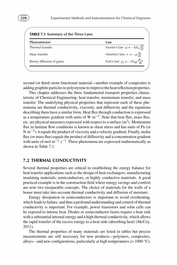
228 Experimental Methods and Instrumentation for Chemical Engineers�
�
�
�
TABLE 7.1 Summary of the Three Laws
Phenomenon LawThermal transfer Fourier’s law: q = −kXA
dTdz
Mass transfer Newton’s law: τ = −μ dudz
Binary diffusion of gases Fick’s law: jA = −DABdCAdz
second (or third) more functional material—another example of composites isadding graphite particles to polystyrene to improve the heat reflection properties.
This chapter addresses the three fundamental transport properties charac-teristic of Chemical Engineering: heat transfer, momentum transfer, and masstransfer. The underlying physical properties that represent each of these phe-nomena are thermal conductivity, viscosity, and diffusivity and the equationsdescribing them have a similar form. Heat flux through conduction is expressedas a temperature gradient with units of W m−2. Note that heat flux, mass flux,etc. are physical measures expressed with respect to a surface (m2). Momentumflux in laminar flow conditions is known as shear stress and has units of Pa (orN m−2): it equals the product of viscosity and a velocity gradient. Finally, molarflux (or mass flux) equals the product of diffusivity and a concentration gradientwith units of mol m−2 s−1. These phenomena are expressed mathematically asshown in Table 7.1.
7.2 THERMAL CONDUCTIVITY
Several thermal properties are critical in establishing the energy balance forheat transfer applications such as the design of heat exchangers, manufacturinginsulating materials, semiconductors, or highly conductive materials. A goodpractical example is in the construction field where energy savings and comfortare now two inseparable concepts. The choice of materials for the walls of ahouse must take into account thermal conductivity and diffusion of moisture.
Energy dissipation in semiconductors is important to avoid overheating,which leads to failure, and thus a profound understanding and control of thermalconductivity is important. For example, power transistors and solar cells canbe exposed to intense heat. Diodes or semiconductor lasers require a heat sinkwith a substantial internal energy and a high thermal conductivity, which allowsthe rapid transfer of the excess energy to a heat sink (absorbing heat) (McCoy,2011).
The thermal properties of many materials are listed in tables but precisemeasurements are still necessary for new products—polymers, composites,alloys—and new configurations, particularly at high temperatures (> 1000 ◦C).

229Chapter | 7 Physicochemical Analysis
7.2.1 Definition
Certain materials, particularly metals, conduct heat rapidly, while others, suchas wood and most plastics and textiles, are poor conductors of heat. The physicalproperty that describes the rate at which heat is conducted (transported) by thematerial is called thermal conductivity and is represented by the symbol k, orsometimes λ.
It is defined by Fourier’s law: the heat flux is a product of the thermalconductivity and a temperature gradient
q = −kdT
dz, (7.1)
where q is the heat flux in W m−2, T is the temperature in K, z is the distancein m, k is the thermal conductivity in Wm−1K, Q = q X A, and X A is the cross-sectional area in m2.
In gases and liquids, transport of heat is through the movement of molecules.In a solid, however, energy is transported by the movement of electrons and thechange in the vibration of the atoms in the lattice. In metals, the movement offree electrons is dominant, whereas in non-metals, the vibration of the ions isthe more important. As shown in Table 7.2, the thermal conductivity of gasesis an order of magnitude lower than that of liquids and some metals are asmuch as three orders of magnitude larger than that of water. Silver has a veryhigh thermal conductivity—a 429 W m−1 K−1—while, surprisingly, two non-metals (diamond and graphene) have an even higher thermal conductivity—asmuch as an order of magnitude higher.
7.2.2 Measurement of Solids
The principle behind the determination of the thermal conductivity of a materialis based on the relationship between the heat flow through the material and theresulting temperature gradient.
Consider a heat flux through surface “A” of a solid plate of thickness �z(see Figure 7.1). Following Fourier’s law, the thermal conductivity of the plateis calculated:
k = − Q�z
X A(T2 − T1). (7.2)
One could easily imagine a heat source on one side of the plate and a sinkon the other that absorbs the energy traversing the object. A practical exampleis a combustion chamber in which the interior is maintained at temperaturesabove 800 ◦C, while the exterior might be close to ambient. Instrumentationmeasuring the thermal conductivity relies on thermocouple readings on eachside of the vessel (or plate, as shown in Figure 7.1). Heat losses from the sidesof the plate should be minimized in to limit heat losses. Thus, the sides may beinsulated or a heat gradient might be added to mimic the axial gradient.
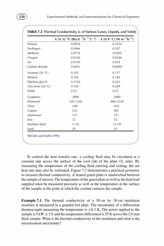
230 Experimental Methods and Instrumentation for Chemical Engineers�
�
�
�
TABLE 7.2 Thermal Conductivity, k, of Various Gases, Liquids, and Solids
k (@ 32 ◦F) (Btu h−1ft−1◦F−1) k (@ 0 ◦C) (W m−1K−1)Helium 0.0818 0.1416
Hydrogen 0.0966 0.167
Methane 0.0176 0.0305
Oxygen 0.0142 0.0246
Air 0.0140 0.024
Carbon dioxide 0.0052 0.0090
Acetone (20 ◦C) 0.102 0.177
Ethanol 0.105 0.182
Ethylene glycol 0.1530 0.265
Glycerine (20 ◦C) 0.164 0.284
Water 0.32 0.55
Graphene 2890 5000
Diamond 520–1340 900–2320
Silver 248 429
Copper 232 401
Aluminum 137 237
Iron 32 55
Stainless Steel 7–26 12–45
Lead 20 35
McCabe and Smith (1976).
To control the heat transfer rate, a cooling fluid may be circulated at aconstant rate across the surface of the cool side of the plate (T2 side). Bymeasuring the temperature of the cooling fluid entering and exiting, the netheat rate may also be estimated. Figure 7.2 demonstrates a practical geometryto measure thermal conductivity. A heated guard plate is sandwiched betweenthe sample of interest. The temperature of the guard plate as well as the heat loadsupplied must be measured precisely as well as the temperature at the surfaceof the sample at the point at which the coolant contacts the sample.
Example 7.1. The thermal conductivity of a 30 cm by 30 cm insulationinsulator is measured in a guarded hot plate. The uncertainty of a differentialthermocouple measuring the temperature is ±0.3 K. The power applied to thesample is 5 kW ± 1% and the temperature differential is 55 K across the 2.0 mmthick sample. What is the thermal conductivity of the insulation and what is themeasurement uncertainty?

231Chapter | 7 Physicochemical Analysis
q
z
T1 T2
FIGURE 7.1 Heat Conduction Through a Plate
Hot plate
Coolant
Coolant
SampleGuard
FIGURE 7.2 Guarded Hot Plate to Measure Thermal Conductivity
Solution 7.1. The surface area of the sample, X A, is 0.09 m2 and the heatrate across the surface, Q, is 5 kW ± 1%, so �Q/Q = 0.01. Introducing thenumerical values in the relationship for thermal conductivity gives:
k = − Q
X A
�z
�T= − 5 kW
0.090 m2
0.002 m
−55 K= 2.02 kW m−1 K−1.
Because the relationship between the thermal conductivity and the measuredvalues can be expressed as a power law, the uncertainty of the conductivity isgiven by:
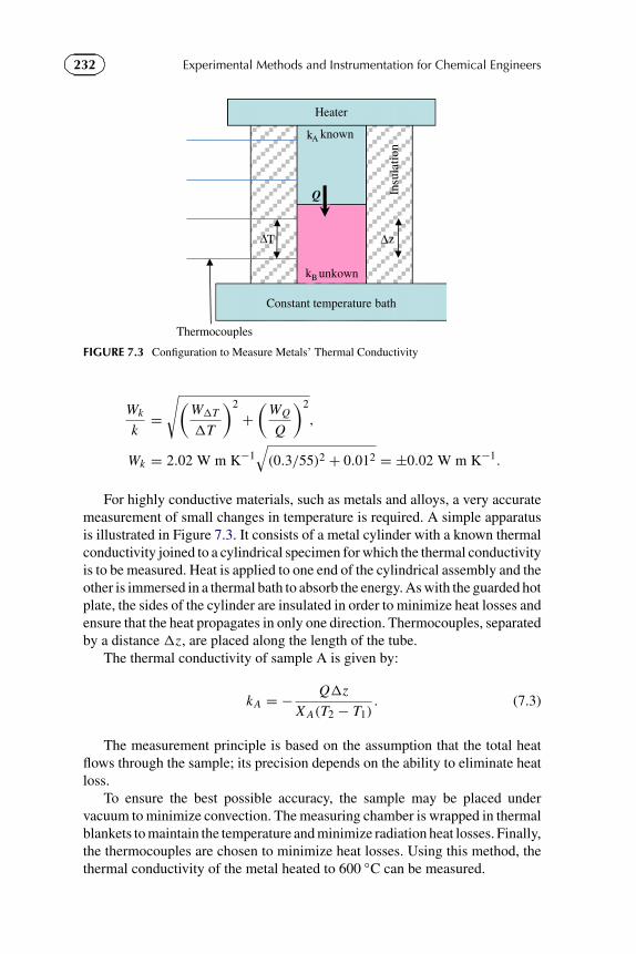
232 Experimental Methods and Instrumentation for Chemical Engineers
Heater
Constant temperature bath
Q
T
kB unkown
Insu
lati
on
Thermocouples
kA known
zΔ Δ
FIGURE 7.3 Configuration to Measure Metals’ Thermal Conductivity
Wk
k=
√(W�T
�T
)2
+(
WQ
Q
)2
,
Wk = 2.02 W m K−1√
(0.3/55)2 + 0.012 = ±0.02 W m K−1.
For highly conductive materials, such as metals and alloys, a very accuratemeasurement of small changes in temperature is required. A simple apparatusis illustrated in Figure 7.3. It consists of a metal cylinder with a known thermalconductivity joined to a cylindrical specimen for which the thermal conductivityis to be measured. Heat is applied to one end of the cylindrical assembly and theother is immersed in a thermal bath to absorb the energy. As with the guarded hotplate, the sides of the cylinder are insulated in order to minimize heat losses andensure that the heat propagates in only one direction. Thermocouples, separatedby a distance �z, are placed along the length of the tube.
The thermal conductivity of sample A is given by:
kA = − Q�z
X A(T2 − T1). (7.3)
The measurement principle is based on the assumption that the total heatflows through the sample; its precision depends on the ability to eliminate heatloss.
To ensure the best possible accuracy, the sample may be placed undervacuum to minimize convection. The measuring chamber is wrapped in thermalblankets to maintain the temperature and minimize radiation heat losses. Finally,the thermocouples are chosen to minimize heat losses. Using this method, thethermal conductivity of the metal heated to 600 ◦C can be measured.
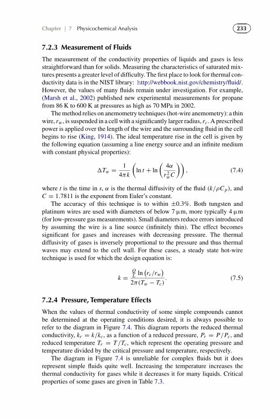
233Chapter | 7 Physicochemical Analysis
7.2.3 Measurement of Fluids
The measurement of the conductivity properties of liquids and gases is lessstraightforward than for solids. Measuring the characteristics of saturated mix-tures presents a greater level of difficulty. The first place to look for thermal con-ductivity data is in the NIST library: http://webbook.nist.gov/chemistry/fluid/.However, the values of many fluids remain under investigation. For example,(Marsh et al., 2002) published new experimental measurements for propanefrom 86 K to 600 K at pressures as high as 70 MPa in 2002.
The method relies on anemometry techniques (hot-wire anemometry): a thinwire, rw, is suspended in a cell with a significantly larger radius, rc. A prescribedpower is applied over the length of the wire and the surrounding fluid in the cellbegins to rise (King, 1914). The ideal temperature rise in the cell is given bythe following equation (assuming a line energy source and an infinite mediumwith constant physical properties):
�Tw = 1
4πk
(ln t + ln
(4α
r2wC
)), (7.4)
where t is the time in s, α is the thermal diffusivity of the fluid (k/ρC p), andC = 1.7811 is the exponent from Euler’s constant.
The accuracy of this technique is to within ±0.3%. Both tungsten andplatinum wires are used with diameters of below 7 µm, more typically 4 µm(for low-pressure gas measurements). Small diameters reduce errors introducedby assuming the wire is a line source (infinitely thin). The effect becomessignificant for gases and increases with decreasing pressure. The thermaldiffusivity of gases is inversely proportional to the pressure and thus thermalwaves may extend to the cell wall. For these cases, a steady state hot-wiretechnique is used for which the design equation is:
k =QL ln
(rc/rw
)2π(Tw − Tc)
. (7.5)
7.2.4 Pressure, Temperature Effects
When the values of thermal conductivity of some simple compounds cannotbe determined at the operating conditions desired, it is always possible torefer to the diagram in Figure 7.4. This diagram reports the reduced thermalconductivity, kr = k/kc, as a function of a reduced pressure, Pr = P/Pc, andreduced temperature Tr = T /Tc, which represent the operating pressure andtemperature divided by the critical pressure and temperature, respectively.
The diagram in Figure 7.4 is unreliable for complex fluids but it doesrepresent simple fluids quite well. Increasing the temperature increases thethermal conductivity for gases while it decreases it for many liquids. Criticalproperties of some gases are given in Table 7.3.

234 Experimental Methods and Instrumentation for Chemical Engineers
Tr
0.3 0.5 1 2 5 10
k r
0.1
0.2
1
5P =P/Pr c
1
1.5
0.82
10
40Saturated Liquid
Pr=0.1
Saturated
vapour
20
5
0.4
FIGURE 7.4 Reduced Thermal Conductivity as a Function of Reduced Pressure and Temperature(Bird et al., 1960, p. 250)
�
�
�
�
TABLE 7.3 Critical Properties of Some Common Gases
Gas Tc (◦C) Pc (atm) Tboiling (◦C)
He −268 2.26 −269
H2 −240 12.8 −253
Ne −229 26.9 −246
N2 −147 33.5 −196
CO −140 34.5 −191
Ar −122 48 −186
O2 −118 50.1 −183
CH4 −83 45.4 −161
CO2 31 72.9 −78
NH3 132 111 −33
Cl2 144 78.1 −34
7.2.5 Insulation Design
Many processes operate at temperatures exceeding 700 ◦C and requireboth specialized metals—stainless steel, Inconel, Hastelloy, etc.—as well asrefractory materials to insulate the metal from the extreme temperatures.Refractory linings and bricks are the most common insulating materials forindustrial vessels. In selecting a refractory lining, its resistance to thermal shock

235Chapter | 7 Physicochemical Analysis
FIGURE 7.5 Refractory Anchors
and mechanical wear, chemical inertness as well as thermal conductivity and thecoefficient of thermal expansion must be considered. Alumina (Al2O3), silica(SiO2), and magnesia (MgO) are the most common insulators. For service atvery high temperatures silicon carbide or graphite can be used but for oxidizingconditions, zirconia is preferred because carbon compounds will oxidize orburn. Figure 7.5 is a photograph of the interior of a 2 m diameter vessel wallillustrating the anchors on which the refractory material is mounted.
New technologies are being developed for ever higher pressure and tem-perature operation. Designing experimental equipment is often as challeng-ing as designing the commercial equipment. The following example illustratesthe design sequence to design a high pressure, high temperature experimentalreactor.
Example 7.2. Propose a refractory and insulation layer design for a 0.0762 mID reactor with an overall length of 0.914 m (36 in.) that is to operate at a max-imum operating pressure and temperature of 35 bar and 1100 ◦C. The vesselis to be made of 304SS (stainless steel) with a maximum external diameter of0.36 m (14 in.). Furthermore, the outer wall temperature should be maintained

236 Experimental Methods and Instrumentation for Chemical Engineers�
�
�
�
TABLE E7.2 Physical Properties of Refractory/Insulating Materials
k (W m−1 K−1) Max Op. Thick. Inc.Temp. (◦C) Avail. (in.)
Alumina refractory 3.00 1930 0.0625
Insulating wool 0.30 1000 0.75
Ceramic paper 0.09 810 0.0625
Microporous insulation 0.04 640 0.25
Stainless steel 16.2 120 0.75
less than 120 ◦C in order to maintain its structural integrity. The reactor is tobe installed in a well-ventilated room at a temperature of 25 ◦C. Table E7.2summarizes the properties of a select number of insulating materials availablefor the project. J.R. Tavares
Solution 7.2. Due to the imposed constraints, the solution to this design prob-lem will be iterative in nature including the following simplifying assumptions:
● Steady state.● Thermal conductivities are constant (no variation with temperature).● Axial and longitudinal conduction are negligible (i.e. conduction only in the
radial direction).● Heat transfer coefficient between the reactor wall and room is 10 W m−2 K−1
(natural convection).● Heat losses due to radiation are negligible.
A common way of approaching problems with multi-layered systems is toconsider each of the layers as a resistance to heat transfer (analogous to electri-cal circuits). In this case, because each refractory/insulating material is layeredonto the previous material, these thermal “resistances” can be considered asbeing “in series” and are thus additive. In heat transfer, the resistance typicallyhas units of temperature over heat rate (such as K W−1).
The heat flow, Q, can be calculated using Fourier’s law of heat transfer incylindrical coordinates:
Q = −k(2πrl)dT
dr,
where k is the thermal conductivity of the pipe material, r is the radius, l is thelength of the pipe, and T is the temperature at a given r.
Integrating from the inner radius, ri , to the outer radius, ro, of a given layergives:
Q = k(2πl)(Ti − To)
ln(ri/ro
) .

237Chapter | 7 Physicochemical Analysis
This equation can be expressed in terms of thermal resistance as follows:
Q = 1
Ri(Ti − To),
in which:
Ri = ln(ri/ro
)ki (2l)
.
Thus, it is possible to obtain the global heat flow out of the reactor by addingup the resistances contributed by each of the layers and using the resulting totalresistance in the heat flow equation.
The challenge in solving the problem lies in the fact that each of the lay-ers is constrained on both the maximum continuous operating temperature andthickness increments. These constraints make it such that the only way to solvethis problem is through trial and error, validating whether or not the operationalconstraints are met for one particular combination and adjusting accordingly.
The available radial space for the refractory/insulating materials is 4.75 in.(7 in. outer radius minus 0.75 in. stainless steel shell minus 1.5 in. inner reactorradius).
As a first guess, we assume the following combination:
● Alumina refractory: 2 in. (32 layers, 0.0508 m).● Insulating wool: 2.25 in. (three layers, 0.05715 m).● Ceramic paper: 0.25 in. (four layers, 0.00635 m).● Microporous insulation: 0.25 in. (one layer, 0.00635 m).
The first step is to calculate the global heat flow. The thermal resistance foreach layer is:
Rrefractory = ln(r2/r1
)krefractory(2πl)
,
Rwool = ln(r3/r2
)kwool(2πl)
,
Rpaper = ln(r4/r3
)kpaper(2πl)
,
Rmicroporous = ln(r5/r4
)kmicroporous(2πl)
,
where r1 = 0.03810 m (inner reaction space), r2 = 0.08890 m (refrac-tory/wool interface), r3 = 0.14605 m (wool/paper interface), r4 = 0.15240 m(paper/microporous interface), r5 = 0.15875 m (microporous/steel interface),and l = 0.914 m.

238 Experimental Methods and Instrumentation for Chemical Engineers
The resistance from the outer stainless steel shell will be:
Rsteel = ln(r6/r5
)ksteel(2πl)
,
where r6 = 0.17785 m (outer vessel radius). And finally, the resistance due tonatural convection will be:
Rconvection = 1
h A= 1
h(2πr6l).
By substituting these values into the heat flow equation, the global heat flowfrom the inner reactor conducted through the various layer and convected outof the system through natural convection is found:
Q = 1
Rrefractory + Rwool + Rpaper + Rmicroporous + Rsteel + Rconvection
× (Ti − To)
with Ti = T1 = 1373 K and To = T6 = 298 K (1100 ◦C and 25 ◦C, respec-tively).
For the proposed combination of materials, the global heat flow isQ = 1762 W.
Conservation of energy dictates that the heat will pass through each ofthe layers. Thus, it is possible to calculate the interfacial temperature betweeneach layer by applying the same heat flow equation, but focusing around asingle thermal resistance. For example, in the case of the alumina refractorylayer:
Q = 1
Rrefractory(T1 − T2),
which can be rearranged to:
T2 = T1 Q Rrefractory.
The same procedure can be repeated for each layer in order to measure theinterface temperature. The values calculated for the proposed combination are:
● Alumina refractory inner temperature T1: 1100 ◦C.● Insulating blanket inner temperature or alumina refractory outer temperature
T2: 1013 ◦C.● Ceramic paper inner temperature or insulating blanket outer temperature T3:
498 ◦C.● Microporous insulation inner temperature or ceramic blanket outer temper-
ature T4: 354 ◦C.

239Chapter | 7 Physicochemical Analysis
● Stainless steel inner temperature or microporous insulation outer tempera-ture T5: 54 ◦C.
● Stainless steel outer temperature T6: 52 ◦C.
In the present configuration, it appears that all temperature constraints aremet except the constraint on the insulating blanket (over by 13 ◦C). Thus theprocedure must be repeated.
If three layers of alumina refractory are added (bringing the refractory thick-ness up to 2.1875 in.) at the expense of three layers of ceramic paper (bringingthe ceramic paper thickness down to 0.0625 in.), the global heat flow Q increasesto 1992.1 W and the new temperature profile is:
● Alumina refractory inner temperature T1: 1100 ◦C.● Insulating blanket inner temperature or alumina refractory outer temperature
T2: 996 ◦C.● Ceramic paper inner temperature or insulating blanket outer temperature T3:
437 ◦C.● Microporous insulation inner temperature or ceramic blanket outer temper-
ature T4: 397 ◦C.● Stainless steel inner temperature or microporous insulation outer tempera-
ture T5: 58 ◦C.● Stainless steel outer temperature T6: 56 ◦C.
This combination respects all the required temperature constraints and,while it is not the only solution, it is noteworthy in that the stainless steeltemperature is far below the maximum safety limit. This is of particular impor-tance considering the fact that the stainless steel shell will be the componentwithstanding the strain of the high operating pressure.
To further refine the design, it would be pertinent to remove the simplifyingassumption that the thermal conductivities of the various layers are constantwith respect to temperature, as this is unrealistic.
Moreover, the proposed solution does not take into account any economicconsiderations. For example, the microporous insulation and the ceramic paperare significantly more expensive than the insulating wool. Also, the solutionproposed uses the maximum allowable steel shell diameter, which may be pro-hibitively costly. Alternative solutions may be possible and less costly, partic-ularly if forced convection (such as a fan) is used to draw additional heat awayfrom the outer reactor wall.
Finally, the proposed design does not take into account the thermal expansionor the compressibility of the various layers, particularly the alumina refractoryfor the former and the insulating wool for the latter. Typical commercial designsmake allowances for such phenomena.

240 Experimental Methods and Instrumentation for Chemical Engineers
7.3 VISCOSITY
The word “rheology” comes from the Greek “Rheos” which means flow. Rheol-ogy studies the deformation and flow of materials in response to the action of aforce. It describes the interrelationship between force, deformation,and time andprovides information on the consistency of materials, by their viscosity—whichis simply the resistance to flow—and elasticity, i.e. structure and/or adhesion.
As an example of an application of rheology, one could cite the measurementof the hydrodynamics of submarine avalanches caused by earthquakes. Thespeed of the avalanche is related to the rheology of the sediments: viscoussediments flow more slowly compared to less viscous avalanches. The speedat which the avalanche proceeds has a direct relationship with the severity ofensuing tidal wave—tsunamis.
The invention of the water clock in 1650 BC in Egypt is arguably the firstquantitative application of rheological principles to a practical application:the viscosity of fluids depends on temperature and Amenemhet took this intoconsideration in his design. He added a 7◦ angle modification to his water clockto account for the viscosity at night versus the day. The first detailed study ofrheology emerged in the late seventeenth century, with the empirical law ofdeformation of Robert Hooke, which describes the behavior of solids. They areoften represented by an elastic spring, whose elongation, ε, is proportional tothe force, σ , applied at its extremity:
σ = Eε. (7.6)
Hooke was seeking a theory of springs, by subjecting them to successivelyincreasing force. Two important aspects of the law are the linearity and elas-ticity. Linearity considers that the extension is proportional to the force, whilethe elasticity considers that this effect is reversible and there is a return to theinitial state, such as a spring subject to weak forces. Hooke’s law is valid forsteels in most engineering applications, but it is limited to other materials, likealuminum only in their purely elastic region.
In 1687, the empirical law of Newton related the flow stress of a fluid to itsvelocity gradient. The constant of proportionality was the viscosity. In fact, theviscosity describes the internal resistance of the fluid to flow and deformation.For example, water has a low resistance to flow, hence its viscosity is lowercompared to most oils, for example, that have a higher resistance (at roomtemperature). Fluids like water and most gases are ideal fluids that satisfyNewton’s theory. Many real fluids have a much more complex relationshipbetween stress, τ , and the velocity gradient,
(dγ /dt
)(γ is the deformation).
The viscosity of Newtonian fluids is represented by the symbol “μ” whereasfor real fluids, it is represented by the symbol “η”, which is also known as thedynamic viscosity:
τ = ηγ . (7.7)

241Chapter | 7 Physicochemical Analysis�
�
�
�
TABLE 7.4 Different Types of Viscosity
Type of Viscosity Symbol and DefinitionRelative viscosity ηrel = (
η/η0) = (
t/t0)
Specific viscosity ηsp = ηrel − 1 = (η − η0/η0
) = (t − t0/t0
)Reduced viscosity (cm3 g−1) ηred = (
ηsp/c)
Inherent viscosity (cm3 g−1) ηinh = (ln ηrel/c
)Intrinsic viscosity (cm3 g−1) [η] = (
ηsp/c)c=0 = (
ln ηrel/c)c=0
u
z
u
b
FIGURE 7.6 Laminar Flow Velocity Profile Between Two Large Plates
For Newtonian fluids, viscosity depends only on pressure and temperature,whereas for non-Newtonian fluids, viscosity also depends on shear rate.
Two hundred years after the early contributions of Newton and Hooke,various laws of real fluids emerged as well as a quantitative description offlow and the measurement of viscosity, including the work of Euler, Cauchy,Coulomb, Poiseuille, Hagen, Couette, Reynolds, and Bingham. In 1890, the firstrotational rheometer was invented by Couette. In 1929, Reiner and Binghamfounded the first rheological society.
Terminology and definitions to characterize viscosity are summarized inTable 7.4.
7.3.1 Single Phase Flow
Consider a fluid contained between two large parallel plates separated by adistance b, as shown in Figure 7.6 and assume that the lower plate is stationarywhile the top plate is driven with a constant velocity u.
When the flow is fully developed (meaning that it is far enough from theentrance—and exit—such that entrance effects have disappeared), the fluidvelocity profile between the two plates is linear and can be defined by thefollowing relationship:
du
dz= u
b. (7.8)

242 Experimental Methods and Instrumentation for Chemical Engineers
FIGURE 7.7 Laminar Flow Velocity Distribution in a Circular Tube
The fluid shear stress, τ , is proportional to the velocity gradient (forNewtonian fluids) and is given by the following equation:
τ = −μdu
dz. (7.9)
In a cylindrical tube with diameter D = 2R and length L, the flow due to thepressure difference (P0−PL) is described by a parabolic profile (see Figure 7.7).
The velocity gradient is given by the Hagen-Poiseuille relation:
du
dr= P0 − PL
2μLr . (7.10)
At r = 0, the flow velocity is maximum and will be linked to the viscosityby the following equation:
umax = P0 − PL
4μLR2. (7.11)
For incompressible fluid flow (fully developed), the volumetric flow rate isreadily calculated as:
V = P0 − PL
8μLπ R4. (7.12)
7.3.2 Reynolds Number
Dimensionless numbers are pure numbers that are expressed as ratios of physicalproperties and are used to classify or understand a system. Already, in Chapter 6,we defined the Reynolds number as the ratio of the fluid’s inertial forces, ρud , toits viscous force and used it to differentiate between the laminar, intermediate,and turbulent flow regimes. In the laminar flow regime, viscous forces dominatebut, as the velocity increases, the Reynolds number increases and inertial forcespredominate in the turbulent regime.
The Reynolds number has been applied to systems other than fluids flowingthrough tubes and pipes; it is used to characterize flow through irregular shaped

243Chapter | 7 Physicochemical Analysis
ducts and even flow of particles through fluids. The form of the equation, for aNewtonian or non-Newtonian fluid, is:
NRe = ρuL
η= uL
ν, (7.13)
where ν is the kinematic viscosity in m2 s−1 (ν = η/ρ) and L is thecharacteristic dimension in m.
The characteristic dimension of fluid flow in a tube is the diameter, d. It is theparticle diameter in fluid-powder systems, dp. In square ducts, it is the hydraulicradius, rH . Note that the notion of turbulence and laminar flow for particles aswell as the values of the Reynolds number are quite different compared to flowthrough pipes and ducts.
The units of viscosity both dynamic, η, and kinematic, ν, are given next.Dynamic viscosity:
1 N s m−2 = 10 P
= 1000 cP
= 1 kg m−1 s−1.
1 P = 100 cP
= 1 dyn s cm−2
= 0.1 N s m−2
= 0.1 kg m−1 s−1.
Kinematic viscosity:
1 St = 1 cm2 s−1
= 100 cSt
= 10−4 m2 s−1.
Example 7.3. Calculate the Reynolds number in a pipeline 1 m in diameter(d ) that transports 100 000 oil barrels per day with a specific gravity of 0.8 anda viscosity 0.2 cP.
Solution 7.3. Pipelines should always be operated in the turbulent flow regimebecause the friction losses are lowest, thus pumping costs are minimized.Furthermore, investment costs will be lower because the cost of pipe pervolumetric flow rate is lower. The volume of one barrel of oil is 159 l. So,the volumetric flow rate of the oil is 15 900 m3 d−1 or 0.184 m3 s−1.
The flow regime is highly turbulent in this example. One risk is that in thewinter the oil could become very viscous if the temperature of the line droppedsignificantly. There exist crude oils with high wax content that are solid attemperatures as high as 50 ◦C. Pipelines carrying these crude oils need to beinsulated to avoid solidification.

244 Experimental Methods and Instrumentation for Chemical Engineers�
�
�
�
TABLE 7.5 Prandtl Numbers and Viscosity of Various Gases and Liquids
Gas/Liquid NPr at 100 ◦C μ, cP at 100 ◦CHelium 0.71 0.02
Hydrogen 0.69 0.01
Methane 0.75 0.04
Oxygen 0.70 0.023
Air 0.69 0.02
Carbon dioxide 0.75 0.017
Acetone 2.4 0.17
Ethanol 10.1 0.32
Ethylene glycol 125 2.0
n-Octane 3.6 0.26
Water 1.5 0.26
McCabe and Smith (1976).
7.3.3 Prandtl Number
The Prandtl number is a dimensionless number that provides a measure of theefficiency of transport by momentum diffusivity to thermal diffusion:
NPr = C pμ
k, (7.14)
where C p is the specific heat in J kg−1 K−1 and μ is the viscosity in kg m−1 s−1.It is also written as the ratio of the kinematic viscosity, ν, which represents
the momentum diffusivity, to the thermal diffusivity, α:
NPr = ν
α= viscous diffusion rate
thermal diffusion rate. (7.15)
The viscous diffusion rate equals the viscosity divided by the density, whilethe thermal diffusion rate is the ratio of the thermal conductivity to the productof fluid density and heat capacity. While the Reynolds number includes a lengthscale, the Prandtl number depends only on fluid properties. The Prandtl numberof many inorganic gases is approximately 0.70, as summarized in Table 7.5.It is much higher for liquids and the variation from one liquid to another isalso greater: the Prandtl number of acetone is 4.5 at 20 ◦C, while it is 350 forethyl ether. It equals 0.015 for mercury. Thermal diffusivity dominates in thecase of mercury. Engine oils have a high Prandtl number and so the convectivecomponent of heat transfer is higher.
For simultaneous heat and mass transfer applications, the Prandtl numberindicates the relative thickness of the momentum boundary compared to the

245Chapter | 7 Physicochemical Analysis�
�
�
�
TABLE 7.6 Viscometry Techniques
Viscometer Range (cP) FluidFalling ball 0.5–70 × 103 Newtonian
Capillary 0.5–105 Newtonian and non-Newtonian
Flow cup 8–700 Newtonian
Rotational 10–109 Newtonian and non-Newtonian
Rolling ball 0.5–105 Newtonian
Drawing ball 0.5–107 Newtonian
thermal boundary layer. (The laminar boundary layer is the region next to asolid surface—temperature, velocity, and concentration gradients are highestin the immediate vicinity of the boundary layer and tend to be zero in the fullydeveloped region.) For low values of the NPr, the momentum boundary layeris smaller than the thermal boundary layer—heat is dissipated more rapidlythan the momentum. When the viscosity is low compared to the ratio of thethermal conductivity to the heat capacity, the momentum boundary layer will besmaller compared to the thermal boundary layer, NPr > 1. The thickness of themomentum boundary layer equals the thermal boundary layers when NPr = 1.
7.3.4 Viscosity Instrumentation
Experimental methods to measure viscosity vary depending on the fluidtype: capillary flow through a vertical tube is the most common method fortransparent, low viscosity fluids (water, organic solvents, etc.); for viscous fluidssuch as oils, molten polymers, gels, etc. rotating concentric cylinders are used.The range of the different techniques is given in Table 7.6.
7.3.4.1 Newtonian FluidsThe falling ball viscometer consists of a tube that may be rotated about a hor-izontal axis, as shown in Figure 7.8. The tube is marked with two lines a and band contains the fluid of interest maintained at a given temperature. A sphere(steel and glass are the most common materials) with a finely calibrated diam-eter is inserted into the tube. At the beginning of the test, the ball lies at thebottom. The tube is rotated by 180◦, which brings the ball (sphere) to the topand then it drops through the fluid. The time it takes to traverse a prescribeddistance L between the lines a and b is measured. The velocity of the ball is thedistance between the two lines divided by the time.
The principle of the falling ball viscometer is similar to that of the rotame-ter (discussed in Chapter 5)—instead of suspending a bob in the flowing gas,the sphere moves at a constant velocity and the fluid is immobile. As with therotameter, the gravitational force on the sphere, Vsρs g, acts downward and the

246 Experimental Methods and Instrumentation for Chemical Engineers
a
bball
L
FIGURE 7.8 Falling Ball Viscometer
buoyancy force, V f ρ f g, and inertial force act upward. So, based on the forcebalance we have:
V ρ f g + CD Ap,sρ fu2
s
2= V ρs g, (7.16)
where V is the volume of the sphere( 4
3π R3),Ap,s is the projected area of the
sphere in m2(π R2),ρs andρ f are the densities of the sphere (s) and the fluid (f) inkg m−3,g is the gravitational constant in m s−2, and CD is the drag coefficient.
In the particle laminar flow regime—also known as the Stokes regime—thedrag coefficient equals 24/NRe. So, the above equations can be simplified toexpress the time of descent, t, as a function of geometry and physical properties:
t = 6π RL
(ρs − ρ f )V gμ = 9
2
L
(ρs − ρ f )R2gμ, (7.17)
where L is the distance between points a and b in Figure 7.8.
Example 7.4. The viscosity of a new polymer formulation is measured in afalling ball viscometer. A total of nine readings are made with a stopwatchfor a 2.00 cm ball to traverse a distance of 0.300 m: 23.5 s, 22.9 s, 24.1 s,21.5 s, 24.5 s, 23.3 s, 22.9 s, 23.7 s, and 23.3 s. The density of the steel ballis 7850 kg m−3 and the polymer density is 852 ± 8 kg m−3. (a) What is itsviscosity? (b) What is the uncertainty?
Solution 7.4.a. Based on the nine experiments, the average time of descentis 23.3 s with a standard deviation of 0.9 s. The radius, R, of the steel ball is0.01 m, and so the viscosity may be calculated directly from the equation:
μ = 9
2L(ρs −ρ f )R2gt = 9
2 · 0.30(7850−852)(0.01)2 ·9.82·23.3 = 160 Pa s.

247Chapter | 7 Physicochemical Analysis
Solution 7.4.b. The uncertainty in the calculated viscosity is due to thecontributions of the uncertainty of the density of the polymer as well as theuncertainty in the measurement of time:
Wμ
μ=
√(W�ρ
�ρ
)2
+(
Wt
t
)2
.
The relationship between the polymer density, ρpoly, and the difference indensity, �ρ, is linear and since only the uncertainty in the polymer density isquoted, W�ρ = Wρ,poly = ±8 kg m−3. The uncertainty with respect to time iscalculated based on the 95% confidence interval:
Wt = ±t(α,n − 1)st = ±t(95%,8)s√n
= 2.3060.85
3= 0.65,
Wμ =√(
8
7000
)2
+(
0.65
23.3
)2
· 160 Pa s ∼= 4 Pa s.
7.3.4.2 The Saybolt ViscometerCalibrated glass capillary columns are commonly used to measure the viscosityof petroleum fluids. The procedures are described in ASTM methods D88,D445, D2170, and D2171 (the latter two are for bitumen, which is an extremelyviscous opaque fluid). The procedure for D445 involves first loading the fluidto the calibrated tube and maintaining it at a constant temperature overnight.The fluid is then brought to just above the highest line in the tube and then itis allowed to drain. The timer is initiated when the bottom of the meniscus justtouches the top line and it is halted when the meniscus touches the bottom line.This procedure is repeated three times. In method D445, the temperature of thebath is kept at 40 ◦C. The bath is then heated to 100 ◦C and the procedure isrepeated.
The Saybolt viscometer works on a similar principle (ASTM D88)—thefluid is loaded to a tube calibrated to 60 ml. A cork is removed from the bottomof a narrow capillary and a timer is initiated. When 60 ml of the fluid is drained,the timer is halted. The time to drain the 60 ml volume is known as “Saybolt”seconds. The instrument operates at temperatures from ambient to as much as99 ◦C. Because of the high sensitivity of viscosity to temperature, substantialefforts are devoted to maintaining isothermal conditions: quoted uncertaintiesaround the temperature are on the order of ±0.03 ◦C. The accuracy of Sayboltviscometers is better than 0.2%. In order to ensure accuracy, they should becalibrated at regular intervals. For fully developed laminar flows, the drain timethrough the capillary at the base is directly proportional to viscosity. However,since the capillary section of the tube is short, a correction factor to the time is

248 Experimental Methods and Instrumentation for Chemical Engineers
Rate of shear strain, du/dz0
Shea
r stre
ss, τ
0
Bingham plastic
Shear thinning
Newtonian
Shear thickening
FIGURE 7.9 Classification of Non-Newtonian Fluids
introduced to account for the fact that the flow profile is not entirely developed:
ν = 0.255t − 208
t. (7.18)
Note that the units of the kinematic viscosity for this equation are in St—cm2 s−1. The importance of the correction term decreases with increasing time.At 100 s, the second term on the right-hand side of the equation represents 8%of the total. Below a value of 28 s, the kinematic velocity equals zero.
7.3.4.3 Non-Newtonian FluidsMost fluids exhibit non-Newtonian behavior—blood, household products liketoothpaste, mayonnaise, ketchup, paint, and molten polymers. As shown inFigure 7.9, shear stress, τ , increases linearly with strain rate, γ , for Newtonianfluids. Non-Newtonian fluids may be classified into those that are timedependent or time independent and include viscoelastic fluids. Shear thinning(pseudoplastic) and shear thickening (dilatant) fluids are time independent whilerheopectic and thixotropic are time dependent. The shear stress (viscosity) ofshear thinning fluids decreases with increasing shear rate and examples includeblood and syrup. The viscosity of dilatant fluids increases with shear rate. Theviscosity of rheopectic fluids—whipping cream, egg whites—increases withtime while thixotropic fluids—paints (other than latex) and drilling muds—decrease their viscosity with the duration of the shear.
7.3.4.4 The Rotational RheometerThe first cylindrical rotary rheometer was invented in 1890 by Couette. Rota-tional rheometers consist of two concentric cylinders, as shown in Figure 7.10.

249Chapter | 7 Physicochemical Analysis
0ω
r2
r1
FIGURE 7.10 Schematic of a Coaxial Rotational Rheometer (Patience et al., 2011)
The test fluid is placed between the cylinders and the inner cylinder is rotatedat a constant velocity ω while the outer cylinder remains fixed. A no-slip con-dition is assumed for the fluid in contact with each wall; therefore, the fluid inthe outer wall is stationary while it rotates at an angular velocity ω0 at the innerwall. Because of the rotational motion, the shear rate, γ , varies across the gapand shear stress.
The torque of the shaft is related to the shear stress τ by the followingequation:
τ = M
2πr2h, (7.19)
where M is the torque of the shaft and 2πr2h is the wetted surface area in m2.
7.3.5 Influence of Temperature and Pressure on Viscosity
Figure 7.11 shows the effect of temperature and pressure changes on viscosity.The reduced viscosity μr = μ/μc is the viscosity at pressure P and temperatureT divided by the viscosity at the critical point, μc. This quantity is shown as afunction of reduced temperature Tr = T /Tc and reduced pressure Pr = P/Pc.

250 Experimental Methods and Instrumentation for Chemical Engineers
Tr
0.5 1 2 5 10
μ r
0.2
1
5
10Pr=P/Pc
1
32
5
10
25
Low density limit
Critical point
Two phase region
Liquid
Pr=0.5
FIGURE 7.11 Diagram of Reduced Viscosity as a Function of Reduced Pressure and Temperature(Bird et al., 1960, p. 16)
For a gas of low density, viscosity increases with increasing temperaturewhile it decreases for a liquid. The relationship is applicable to low molecularweight Newtonian fluids.
7.4 BINARY GAS DIFFUSION
The transport of chemical species from a region of high concentration to a regionof low concentration can be demonstrated experimentally by the diffusion ofa crystal of potassium permanganate (KMnO4) with water in a beaker. TheKMnO4 begins to dissolve in water, a dark purple halo first forms aroundthe crystal (region of high concentration) and then diffuses over time due tothe concentration gradient, until the equilibrium concentration is reached.
Diffusion is the spontaneous movement of a species under the effect of aconcentration difference, or in other cases, a gradient of temperature or force(electrostatic force in the case of charged species or chemical potential).
Diffusion is described mathematically by Fick’s first law (1855),demonstrating that the net movement of a species through a unit area (flux)is proportional to the concentration gradient. The constant of proportionality iscalled the diffusion coefficient D, or diffusivity.
The applications of this law are numerous, but only a few examples will begiven here. Take first our body as an example. Our lungs are made up of verythin cells (less than a millionth of a meter) and have a large effective area (about100 m2) that facilitates the exchange of gases, which depends on the diffusionand the solubility of the fluid in the membrane of the lungs. The transport ofmolecules through the pores and channels in the membrane of our cells as well

251Chapter | 7 Physicochemical Analysis
as the transport of oxygen and carbon dioxide in the blood both proceed throughdiffusion.
A second example concerns packaging in the food industry. The effective-ness of thin transparent wrapping (polymers) in protecting food depends on theirability to prevent the spread of pathogenic microorganisms, external moisturecausing mold, and oxygen responsible for the oxidation of food.
Finally, in the field of construction, increasing the temperature andconcentration of carbon dioxide in the atmosphere has a significant impacton the life of urban structures in concrete. Moreover, the structures in a marineenvironment are damaged mainly by chloride ions. The evaluation of theirservice life is based on the determination of the penetration of these ions inconcrete, that is to say, by calculating their diffusion coefficient, with Fick’s law.
7.4.1 Fick’s Law
Considerable research is devoted to high performance Sportswear and even theReady-to-Wear segments of textiles. The desire is to maintain the body dryby wicking water away as the body generates heat and perspires. To illustratethe concept of diffusion, consider a semi-permeable membrane laminated to afabric. Assume the sample was placed in a cell separating a column of air froma column of saturated water vapor. The membrane is permeable for water vaporbut not air. At time t = 0, thanks to Brownian motion, the water moleculeswill traverse the membrane and then diffuse through the fabric sample to theair. (Evidently, the fabric sample is usually next to the skin—this example isfor illustration purposes only.) The molecular transport through the fabric isreferred to as diffusion.
In this system, we designate water as species A and air is referred to as speciesB. The mass fractions are denoted by xA and xB and they are defined as themass of the individual species divided by the sum of the masses of the species.The molar fractions yA and yB equal the moles of species A or B with respectto the total number of moles. Remember that the total molar density equals P
RTfor gases. Figure 7.12 demonstrates the evolution of the mass fraction of wateras a function of time. The first vertical solid line represents the semi-permeablemembrane. The fabric extends from the membrane to the dotted line. Initially,the mass fraction of water in the fabric equals zero. At the beginning of theexperiment, the mass fraction of water at the membrane equals one and it iszero in the fabric. As time advances, the mass fraction in the fabric increases(third image from the top). With time, the concentration profile of species Aeventually becomes a straight line, as shown in Figure 7.12.
The mass flux of species A in the direction of z is given by Fick’s law:
jA = −ρDABdxA
dz, (7.20)
where DAB is the mass diffusivity of species A in species B in m2 s−1.

252 Experimental Methods and Instrumentation for Chemical Engineers
xA= xA0
t = 0xA= xA0
t < 0
xA
1
0
1
0
1
0
t = ∞
t > 0xA(y,t )
xA(y,∞)
xA= 0
1
0
z
FIGURE 7.12 Diffusion of A Through a Semi-Permeable Membrane (Solid Line) Through aFabric (Up to Dotted Line)
7.4.2 Schmidt Number
The Schmidt number is a dimensionless number equal to the ratio of kinematicviscosity to mass diffusivity. It is:
NSc = ν
DAB= ρ
η
DAB. (7.21)
7.4.3 Measure of Diffusion
The device illustrated in Figure 7.13 is used to measure the diffusion coefficientof binary gas pairs. Two glass tubes with equal cross-sections are joined togetherat one end with a flexible tube that is pinched in the middle. Each tube is filledwith a different gas and the clip is detached to initiate the experiment (t = 0).
The gases begin to diffuse due to the concentration gradient. After aprescribed time, the flexible tube is rejoined and the concentration of gas in eachtube is determined. It would be sufficient to measure the concentration of oneside to know what the concentration of the other side of the column should be.Good experimental practice would sample both columns to evaluate themeasurement error.
The concentrations of both gases are given by the following equation:
F = NA1 − NA2
NA1 + NA2= 8
π2
∑k=0
1
(2k + 1)2 exp
(−π2 DABt(2k − 1)2
4L2
),
(7.22)where 1 and 2 are the upper and lower tubes, t is the time of the experiment,L is the length of the tube, NA1 is the number of moles of A in the upper tube,and NA2 is the number of moles of A in the lower tube.

253Chapter | 7 Physicochemical Analysis
(1)
(2)
Flexiblehousing
L
L
FIGURE 7.13 Loschmidt Instrument to Measure Gas Diffusion Coefficients (Holman, 2001)
The optimum time to run the experiment to determine DAB is calculatedfrom the following equation:
topt = 4L2
π2 DAB. (7.23)
The equation to calculate the factor F involves series terms. When theexperiment is run up to topt, the higher-order terms may be neglected. Thus,the diffusion coefficient may be determined from the following equation:
DAB = −4L2
π2tln
(π2 F
8
). (7.24)
Measuring diffusion rates is quite uncommon. Rather, the expected diffusionrates are calculated based on empirical relationships such as the following:
P DAB
(PcA PcB)1/3(TcATcB)5/12√
1MA
+ 1MB
= a
(T√
TcATcB
)b
, (7.25)

254 Experimental Methods and Instrumentation for Chemical Engineers�
�
�
�
TABLE 7.7 Binary Diffusivity Pairs
Pairs A–B Temperature (K) Diffusivity, DAB (cm2 s−1)CO2–N2 273.2 0.144
H2–CH4 298.2 0.726
H2O–N2 308 0.259
H2O–O2 352 0.357
He–Pyrex 283.2 4.5 × 10⁻¹⁰
Hg–Pb 283.2 2.5 × 10⁻¹⁵
Al–Cu 283.2 1.3 × 10⁻³⁰
Bird et al., 2006, p. 503.
where P is the pressure in atm, Pc is the critical pressure in atm, Tc is the criticaltemperature in K, M is the molecular weight in kg kmol−1, a is 2.745 × 10⁻⁴
for nonpolar gas pairs and 3.640 × 10⁻⁴ for water into nonpolar gases, and bis 1.823 for nonpolar gas pairs) and 2.334 for water into nonpolar gases.
At pressures close to atmospheric, this equation agrees with experimentaldata to within 8%. Table 7.7 summarizes the diffusivity of various binary pairs-gas-gas, gas-solid and solid-solid.
7.4.3.1 Water Vapor Diffusion Through MembranesMeasuring water vapor transmission through membranes has been an activearea of research for several decades now. Applications not only include textiles,but also housing, footwear, food packaging, and other industrial uses. The testsproposed in this section will be applied to measure the permeability of samplesexceeding 32 mm thickness. There are two basic methods given by the ASTM:
1. Method using hygroscopic powder (ASTM E96-00):A film (membrane) is mounted on a sealed cup containing calcium chlo-ride dried before-hand at 200 ◦C (or another hygroscopic powder). Theanhydrous calcium chloride should have a particle size between 600 µmand 2.36 mm. The cup should be made of a light material that is imper-meable to water vapor. The opening of the cup, over which the film ismounted, should be on the order of 3000 mm2. The distance between thetop of the anhydrous CaCl2 and the film should be approximately 6 mm.(It is important to avoid touching the film with the powder.) The assem-bly is placed in an environmental chamber where the temperature and rel-ative humidity should be checked frequently (temperature from 21 ◦C to23 ± 1 ◦C and relative humidity at 50% ± 2%). Air must circulate continu-ously at a velocity of up to 0.3 m s−1.

255Chapter | 7 Physicochemical Analysis
The cup assembly should be weighed at regular intervals until a con-stant value is achieved to determine the rate of absorption of water vaporby the CaCl2. (For this reason, the cup should be made out of light—andimpermeable—materials.) The weight scale should have a sensitivity wellbelow 1% of the total weight of the cup plus the powder.
2. Method using water (ASTM E96-00):The operating conditions of this test are similar to those of the test with thehygroscopic powder. However, in this case, the cup is filled with water andthe rate of water transmission is calculated based on the drop in the weightof thecupandwaterassembly.Figure7.14 illustrates thewaterbath intowhichthecupsareplaced toachieveauniformtemperature.Note that this instrumenthas room for 12 cups. In this way, many measurements can be made simulta-neously and be either used to test many samples or to evaluate the uncertaintyin the measurement of a single sample or even multiple samples.
Each cup should be filled with distilled water such that the space betweenthe water level and the sample is from 13 mm to 23 mm. The level in the bot-tom of the cup should be on the order of 30 mm but the minimum specifieddepth is 3 mm.
The water vapor transmission rate, WVT, is calculated based on a massbalance:
WVT = �Wc+ f
X At, (7.26)
where X A is the cross-sectional area of the cup opening in m2, �Wc+ f is theweight change of the cup plus the film in g, and t is the time in h.
Front View
Top View
FIGURE 7.14 Device for Measuring the Permeability of Water Vapor

256 Experimental Methods and Instrumentation for Chemical Engineers�
�
�
�
TABLE 7.8 WVP—Water Vapor Permeability of Selected Materials(g m−2 d−1 )
Material Permeability ClassificationSports films (e.g. Gore) >5000
Sports wear (and film) >2400 Very high
Suede >1200 Very high (for leather)
Coated leather 600–1200 High
PU and fabric 240–600 Moderate
PVC and fabric <120 Low
The water vapor permeability, WVP, is calculated based on the water vaportransmission rate:
WVP = WVT
�P= WVT
Psat(RH1 − RH2), (7.27)
where �P is the pressure difference of water vapor (1 mmHg = 1.333 ×10² Pa)),RH1 is the relative humidity in the vapor space of the cup below thefilm, RH2 is the relative humidity in the climate-controlled room, and Psat is thesaturation pressure of the water vapor at the temperature of the cup in mmHg.
Some values of permeability for common materials are summarized inTable 7.8.
The relative humidity in the hygroscopic powder is nominally 0%, while indistilled water, it is 100%.
The saturated water vapor pressure may be calculated according to:
Ps = 610.78 exp
(17.2694T
T + 238.3
), (7.28)
where T is the temperature in ◦C and P is the water vapor pressure in Pa (seeFigure 7.15).
Note: The conditions of temperature and relative humidity must be reportedaccurately for each permeability measurement. Other devices with infrared orcolorimetric detectors may also be used to measure the permeability of the filmsto water vapor.
7.4.4 Temperature and Pressure Influence on the Diffusivityof Gases and Liquids
For a binary gas at low pressure, DAB is inversely proportional to the pressureand increases with increasing temperature. Diffusivity is almost independent ofthe composition of the pair AB.

257Chapter | 7 Physicochemical Analysis
FIGURE 7.15 Mole Fraction of Water as a Function of Temperature (at 1 atm)
Tr
0.5 1 2 5
Red
uced
sel
f-diff
usiv
ity
0.4
0.6
0.8
1
1.5
2
3
Low-pressure limit
Saturated Liquid
Two phaseregion
Vapour
Pr=2
Pr=5
Pr=10
FIGURE 7.16 Diagram of Reduced Self-Diffusivity (Bird et al., 2006, p. 522)
At high pressure in liquids, the behavior of DAB is more complex. However,it is easier to obtain experimental data for self-diffusivity (inter-diffusion ofmolecules within the same chemical species) of nonpolar solutions DAA∗.
Figure 7.16 shows that the self-diffusivity cDAA∗ increases strongly withtemperature, especially for liquids. For each temperature, it decreases to zerowith increasing pressure. This diagram shows the reduced self-diffusivity, whichis the ratio cDAA∗ to pressure P and temperature T divided by the self-diffusivityreduced to the critical pressure Pc and the critical temperature Tc. This quantity

258 Experimental Methods and Instrumentation for Chemical Engineers
is described in terms of the reduced temperature Tr = T /Tc and reducedpressure Pr = P/Pc.
7.5 EXERCISES
7.1 The Governor of Syracuse chose you to replace Archimedes, who diedafter the siege by the Romans (212 BC). The Governor bought 20 beadsof 22-karat gold, which are 1 cm in diameter. He suspects that there is lessthan 75% gold in the beads. Determine if the beads are at least 18 karats(assuming that the other metal is lead)
X = 24Mg
Mm,
where X is the karat rating, and Mg and Mm are the mass of goldand the total mass, respectively. Also, ρAu = 19 200 kg m−3 andρPb = 14 300 kg m−3.
The specific gravity of the oil in the drop ball viscometer is 0.8 and itsviscosity equals μ = 10 000 ± 500 cP. A persons pulse is used as atimer with a rate of 60 beats per minute and an uncertainty of 2 beats perminute. The falling ball drops a distance of 20 cm but the uncertainty ofthe measurement is ±1 cm. The experimenta is repeated five times andthe number of beats each time is: 21, 20, 23, 22, 22.
(a) What should be the speed of a pure gold bead?(b) What is the uncertainty for the measure of speed of the pure gold?(c) Calculate the density of a bead.(d) Calculate the content of gold (in karats) in a bead.(e) Is there less than 75% gold in the beads?(f) The Governor wants to know with more certainty the amount of gold
(or it is your skin that is in danger and not your brother-in-law’s) andasks you to offer three ways to improve the measurement accuracyof the gold content with this device.
7.2 A Saybolt viscometer measures the viscosity of an oil with ν = 50 cSt.What must the uncertainty in the measured time to drain be so that theuncertainty of ν is less than 1%.
7.3 You develop a new insulation (glass wool type) which has a thermal con-ductivity of about 0.05 W m−1 K−1. The insulation is compressible—thus, while preparing the sample you must be careful not to move it. Youplace the sample, with a thickness of about 10 cm, and you apply a heatflux as the temperature difference across the sample is (15.0 ± 0.2) ◦C.

259Chapter | 7 Physicochemical Analysis
(a) If the uncertainty of heat flow is 1%, what should the uncertaintyin the measurement of the thickness of the material be, so that thethermal conductivity is less than ±5%?
(b) If you double the heat flow, what would be the difference in tem-perature?
(c) If you notice a difference of 33 ◦C in (b), give two hypothesesexplaining the difference between this and the one you calculated.
7.4 A cylindrical rod has a cross-section of 5.0 mm2, which is made byjoining a rod of 0.30 m silver to a rod of 0.12 m nickel. The silver sideis maintained at a temperature of 290 K and the nickel side at 440 K.The thermal conductivity of silver is 0.42 kW m−1 K−1 and the thermalconductivity of nickel is 91 W m−1 K−1. Calculate: M. Hu
(a) The steady-state temperature.(b) The rate of conduction of heat down the rod (state any necessary
hypotheses).
7.5 A rod is placed in an instrument to measure thermal conductivity, asshown in Figure 7.3. The thermal conductivity kA of the calibration rodequals 0.5 W m−1 K−1. Calculate kB for the case where the lengths ofboth rods are equal and the temperatures at the heater, bath, and interfacebetween the rods are Th = (40.00 ± 0.02) ◦C,Tb = (20.00 ± 0.02) ◦C,and T�B = (22.50 ± 0.05) ◦C. What is the uncertainty? R. Boutrouka
7.6 A gaseous mixture composed of CH4 and O2 is stored in a large roomat 15 atm and −20 ◦C. Calculate the diffusion coefficient of oxygen inmethane in the room. É. Nguyen
7.7 In the framework of a project on a process of fermentation, a chemicalengineer focuses on heat transfer in a wall of his process which continu-ously circulates a refrigerant. The refrigerant is kept at a temperature of25 ◦C and the temperature difference between coolant and the walls cal-culated by thermocouples indicates 52 ◦C. The sample used to estimatethe heat transfer has a thickness of 15 mm and a diameter of 25 mm andthe power applied to this sample is 7 kW. É. Noiseux
(a) Is it possible to determine the thermal conductivity?(b) If the wall is insulated, determine the thermal conductivity.
7.8 What is the Reynold’s number in a human capillary of 37 ◦C with a vis-cosity of 14 × 10−3 Pa s, a density of 1053 kg m−3, and circulating120 cm s−1? A capillary has a radius of 4.5 µm. A.L. Fakiris
7.9 A Saybolt viscometer was used to calibrate the physical parameters of afalling ball viscometer. Methanol was chosen as the test fluid and its den-sity equaled 792 kg m−3. The drainage time in the Saybolt viscometerwas 30.1 s, and it was 92.1 s in the falling ball viscometer. The diameter

260 Experimental Methods and Instrumentation for Chemical Engineers
of the ball was 2 cm and the distance traveled was 0.3 m. The flow in theSaybolt viscometer was laminar: L.M.K. Fondjo
ν = 0.00237t − 1.93
t,
where ν is in 10−3 ft2 s−1.
(a) Determine the density of the ball.(b) Explain (without calculating) how the students could determine the
uncertainty of the calculated value in (a).
7.10 A parallel plate rheometer is used to characterize the viscosity of a moltenpolymer sample. The rheometer is made of two rectangular parallel platesof dimensions 60 cm × 10 cm that are separated by a 2 mm gap. Theplates are located inside an oven to allow measurements at high temper-ature. The lower plate is stationary, while the upper plate is moving at avelocity V = 10−3m s−1. For the sample investigated, the force requiredto maintain the upper plate velocity at 10−3 m s−1 is 100 N. M.C. Heuzey
(a) What is the shear rate γ applied on the polymer sample?(b) What is the viscosity of the polymer sample?(c) If the velocity of the upper plate is decreased by half, i.e. V =
0.5 × 10⁻³m s−1, the force decreases to 80 N. Is this behaviortypical of molten polymers?
7.11 (a) Water and air are transported through two identical pipes at the samevelocity. Which pipe operates at a lower Reynolds number?
(b) True or false, the advantages of an orifice compared to a venturi are:
(i) It takes less space.(ii) It is easier to calibrate.(iii) There is a permanent and smaller loss of charge.
(c) True or false:
(i) The loss of charge in a Coriolis is less than in a venturi.(ii) The pitot tube can be used to measure the speed of a plane.(iii) The vortex has the least charge loss, takes less space compared
to most flow meters, and varies linearly with flow.
(d) Associate the terms in Table Q7.11 with their correct definition.(e) True or false, the diffusion coefficient:

261Chapter | 7 Physicochemical Analysis�
�
�
�
TABLE Q7.11 Terms and Definitions
Quantity Definition(1) NRe (A) Relationship between the diffusivity of the quantity of
movement and the thermal diffusivity.
(2) NPr (B) Relationship between the diffusivity of the quantity ofmovement and the mass diffusivity.
(3) NSc (C) Relationship between the inertial forces and the viscousforces.
(4) NMa (D) Ratio of the speed (fluid/object) to the speed of sound.
(i) Increases with pressure.(ii) Increases with the square of temperature.(iii) Is higher for H2O–N2 than for H2O–O2.(iv) Varies more with temperature for NH3 than oxygen.
(f) Place the following materials in increasing order of thermal con-ductivity: gases, pure metals, alloys, liquids, and plastics.
(g) True or false:
(i) Helium is preferred to argon for window insulation.(ii) The heat flux equation by conduction is derived from Fourier’s
equation.(iii) Heat propagates in solids, fluids, and in void.
7.12 The thermal conductivity of a sample, shown in Figure Q7.12a, is sand-whiched between two blocks with known thermal conductivities. A con-stant heat flow of Q = 10 J s−1 is applied to the surface of plate A andthe temperature of the outer surface of plate C is measured. The resultsof four experiments with the unknown sample.
A B C
T1T0 T2 T3
k1 kB k1
5 cm Δx
Q
W = 5 cm
H = 10 cm
FIGURE Q7.12 Thermal Conductivity of Sample Setup

262 Experimental Methods and Instrumentation for Chemical Engineers�
�
�
�
TABLE Q7.12a Thermal Conductivity of Sample B
Exp. �x (cm) T1 (◦C) T3 (◦C)
1 1 120 83
2 2 120 72
3 4 120 58
4 5 120 45
�
�
�
�
TABLE Q7.12b Thermal Conductivity and Interval of Confidence
α (%) 90 95 99 99.9
t(α,N),N = 4 2.02 2.57 4.03 6.86
K (α) 1.64 1.96 2.57 3.3
(a) Calculate T2 in each of the experiments.(b) Estimate kB in each of the experiments.(c) The uncertainty in the measurement of the temperature is 1 ◦C and
that of the measurement of the thickness of plate B is 1 mm. Whatis the uncertainty in the value of the thermal conductivity of eachsample B?
(d) Based on Table Q7.12b, calculate the interval of confidence of theestimated thermal conductivities when α = 95%. Comment on thisvalue compared to those calculated in (c).
(e) Should we reject some of the experiments? Why?
7.13 You measure the viscosity of a new polymer in a falling ball viscometer.The density of the polymer is (970 ± 20) kg m−3. The ball is made oftitanium (ρ = 4540 kg m−3) with a radius of 10.0 mm and it travels adistance of 0.40 m.
(a) What are the average and the standard deviation of the experimentaldata?
(b) What is the viscosity?(c) What is the confidence interval for the time measurement?(d) What is the uncertainty in the measurement of the viscosity?(e) Could we reject a data point?
263Chapter | 7 Physicochemical Analysis
REFERENCES
Bird, R.B., Stewart, W.E., Lightfoot, E.N., 1960. Transport Phenomena. John Wiley & Sons.Bird, R.B., Stewart, W.E., Lightfoot, E.N., 2006. Transport Phenomena. John Wiley & Sons.McCoy, M., BASF hikes insulating material capacity, 2011. C&E News, 89 (46).Morazain, J., L’avoin de 2025, 2011. Plan, Nov., 14–18.Elsevier, 2007, December 18. Top 10 Advances in Materials Science Over Last 50 Years.
ScienceDaily. Retrieved June 22, 2011, from: <http://www.sciencedaily.com/releases/2007/12/071218101208.htm>.
Holman, J.P., 2001. Experimental Methods for Engineers, seventh ed. McGraw-Hill, Inc.,New York.
Karayianni, E., Coulston, G.W., Micka, T.A., 2008. Patent no. US2008176073-A1 and Patent no.US7665288-B2.
King, L.V., 1914. On the convection of heat from small cylinders in a stream of fluid, withapplications to hot-wire anemometry. Philosphical Transactions of the Royal Society of London214 (14), 373–433.
Marsh, K.N., Perkins, R.A., Ramires, L.V., 2002. Measurement and correlation of the thermalconductivity of propane from 86K to 600 K at pressure to 70MPa. Journal of Chemical andEngineering Data 47, 932–940.
McCabe, W.L., Smith, J.C., 1976. Unit Operations of Chemical Engineering, third ed. McGraw-HillChemical Engineering Series. McGraw Hill.
Patience, G.S., Hamdine, M., Senécal, K., Detuncq, B., 2011. Méthodes expérimentales etinstrumentation en génie chimique, third ed. Presses Internationales Polytechnique.
Chapter 8
Gas and Liquid Concentration
8.1 OVERVIEW
Species concentration is a critical parameter for the control and safety ofchemical processes, as well as dosing medication (pharmaceuticals) andmundane daily tasks like cooking; the most basic physiological function—breathing—relies on the carbon dioxide concentration in the blood. Air pollutionis measured in terms of concentration of particulates or ozone. Mosquitoesseek their prey through a concentration gradient. The odor threshold of H2S is0.47 ppb. It irritates the eyes at 10–20 ppm and it is lethal at 800 ppm to 50% ofthe population when exposed for a period of 5 min. Properties of chemicalsare listed on Material Safety Data Sheets (MSDS) and include physicalcharacteristics—density, appearance, solubility, vapor pressure, boiling point,etc.—as well as toxicity and flammability characteristics. Toxicity is reported interms of LC50 and LD50. LC50 represents the concentration at which 50% ofthe test specimens die after a period of time. The acute toxicity of isopropanolvapors (LC50) is 16 000 mg l−1 in 8 h for rats. The LC50 for H2S is 800 ppmafter 5 min for humans. Another term used to express toxicity is LD50—thelethal dose at which 50% of the animal population dies. The acute oral toxicity(LD50) of isopropanol for mice is 3600 mg kg1 after a 4-h exposure. Its acutedermal toxicity (LD50) for rabbits is 12 800 mg kg1 after a 4-h exposure.
In this chapter we discuss only a few of the more common instruments usedto assess species concentration including chromatography, mass spectrometry,refractometry, spectroscopy, and X-ray.
8.2 CHROMATOGRAPHY
Co-authors: Danielle Béland, Cristian Neagoe
Experimental Methods and Instrumentation for Chemical Engineers. http://dx.doi.org/10.1016/B978-0-444-53804-8.00008-3© 2013 Elsevier B.V. All rights reserved. 265

266 Experimental Methods and Instrumentation for Chemical Engineers
Solution
FIGURE 8.1 Example of Column Chromatography
Chromatography is a separation technique that was discovered by theRussian botanist Mikhail Semyonovich Tswett during the early 20th century(1903). He separated chlorophyll pigments dissolved in a mixture of petroleumether and ethanol in a column of calcium carbonate (Figure 8.1). The differentpigments with different degrees of affinity for calcium carbonate separated andeluted at different speeds. Chromatography is a contraction of two words fromGreek: chroma (color) and graphein (to write).
Separating compounds in an unknown stream is achieved through theirpreferential adsorption (affinity), partition, on a column (stationary phase). Themore affinity a compound has for the stationary phase, the more it will beretained, which results in a longer retention time. Compounds with low affinityelute first, followed sequentially by the compounds with a greater affinity.Retention time is the primary factor used to identify compounds: compoundseluting from the column are compared to a standard (using the samemethodology). A further confirmation of the identity of the compound is toadd a known quantity of the suspected compound together with the unknownstream to verify that the unknown peak increases. This verification is onlyrequired when matrix effects are suspected—the peaks may be shifted dueto the presence of the other compounds in the stream. The third step ofthe process is to quantify the concentration, which is accomplished withexternal calibration, internal calibration, percent normalization, or standardaddition.
Other types include column chromatography, paper chromatography,thin layer chromatography (TLC), high-performance liquid chromatography(HPLC), gas chromatography (GC), supercritical fluid chromatography (SFC)

267Chapter | 8 Gas and Liquid Concentration�
�
�
�
TABLE 8.1 Different Forms of Chromatography
Stationary Phase Mobile Phase Type of Chromatography
Solid Liquid Liquid/Solid
Solid Gas Gas/Solid
Liquid Liquid Liquid/Liquid
Liquid Gas Gas/Liquid
101 102 103 104 105
Mm, g gmol-1
HPLC
106
GC
HPGPC Traditional GPC
FIGURE 8.2 Applications of Chromatography
and size exclusion chromatography (SEC). The most common, which aretreated in this chapter, are gas chromatography and high-performance liquidchromatography.
Chromatography is an analytical technique used for the separation,identification, and quantification of different compounds in a mixture. Theseparation is the result of the interaction between the different compounds witha stationary phase (liquid or solid) and the mobile gas phase (GC) or liquidphase (HPLC) (Table 8.1).
Applications of chromatography are given in Figure 8.2. Volatile and semi-volatile compounds are analyzed by GC and non-volatiles by HPLC. Sometimesthe process of derivatization is used to increase the volatility of the compoundsso they can be analyzed by GC. HPLC can also be used for thermolabilecompounds and ionized products. SEC separates analytes based on physicaldimensions (hydrodynamic volume or size), whereas the other techniques relyon chemical and physical interactions between the analyte and column. Thedistribution of molecular weight of polymers and protiens are determined byGel Permeation Chromatography (GPC—a class of SEC). High PerformanceGel Permeation Chromatography (HPGPC) is applicable for compounds withmolecular weights on the same order as HPLC.
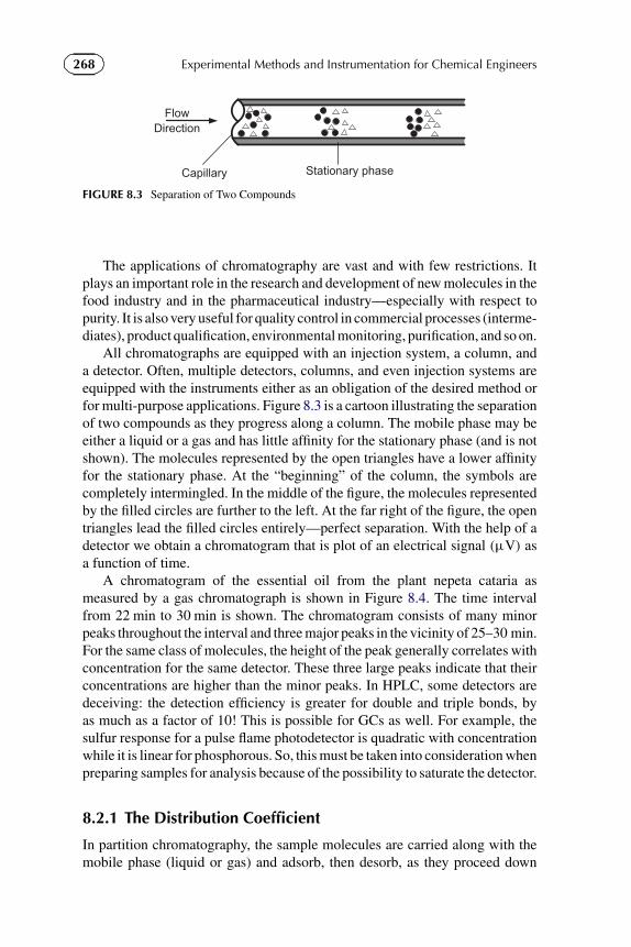
268 Experimental Methods and Instrumentation for Chemical Engineers
Capillary Stationary phase
FlowDirection
FIGURE 8.3 Separation of Two Compounds
The applications of chromatography are vast and with few restrictions. Itplays an important role in the research and development of new molecules in thefood industry and in the pharmaceutical industry—especially with respect topurity. It is also very useful for quality control in commercial processes (interme-diates), product qualification, environmental monitoring, purification, and so on.
All chromatographs are equipped with an injection system, a column, anda detector. Often, multiple detectors, columns, and even injection systems areequipped with the instruments either as an obligation of the desired method orfor multi-purpose applications. Figure 8.3 is a cartoon illustrating the separationof two compounds as they progress along a column. The mobile phase may beeither a liquid or a gas and has little affinity for the stationary phase (and is notshown). The molecules represented by the open triangles have a lower affinityfor the stationary phase. At the “beginning” of the column, the symbols arecompletely intermingled. In the middle of the figure, the molecules representedby the filled circles are further to the left. At the far right of the figure, the opentriangles lead the filled circles entirely—perfect separation. With the help of adetector we obtain a chromatogram that is plot of an electrical signal (µV) asa function of time.
A chromatogram of the essential oil from the plant nepeta cataria asmeasured by a gas chromatograph is shown in Figure 8.4. The time intervalfrom 22 min to 30 min is shown. The chromatogram consists of many minorpeaks throughout the interval and three major peaks in the vicinity of 25–30 min.For the same class of molecules, the height of the peak generally correlates withconcentration for the same detector. These three large peaks indicate that theirconcentrations are higher than the minor peaks. In HPLC, some detectors aredeceiving: the detection efficiency is greater for double and triple bonds, byas much as a factor of 10! This is possible for GCs as well. For example, thesulfur response for a pulse flame photodetector is quadratic with concentrationwhile it is linear for phosphorous. So, this must be taken into consideration whenpreparing samples for analysis because of the possibility to saturate the detector.
8.2.1 The Distribution Coefficient
In partition chromatography, the sample molecules are carried along with themobile phase (liquid or gas) and adsorb, then desorb, as they proceed down

269Chapter | 8 Gas and Liquid Concentration
FIGURE 8.4 Chromatogram of the Essential Oil of Nepeta cataria
the column. The longer the molecule remains adsorbed on the stationary phase,the longer is its retention time. The equilibrium between the concentrationin the mobile phase, Cm , and in the stationary phase, Cs , may be expressed asa ratio, which is known as the distribution coefficient, K D:
Cm ←→ Cs,
K D = Cs
Cm. (8.1)
The retention times of each solute can be determined for each columnknowing the distribution coefficient. The concentration in the mobile phaseis always much smaller than in the stationary phase (Cm � Cs) so K D � 1.Greater values of the distribution coefficient indicate greater solute retention andlonger retention times. The value of K D must be different for two compoundsto be able to separate them.
The separation depends on several criteria:
1. Nature of the solute.2. Nature of the stationary phase.3. Temperature of the column.4. Amount of stationary phase.5. Linear speed of the mobile phase.6. Column length.
8.2.2 The Capacity Factor
The capacity factor, or retention factor, k′, expresses the speed of the passageof solute through the column. The k′ factor determines the residence timeof the solute in the stationary phase compared to the residence time in the

270 Experimental Methods and Instrumentation for Chemical Engineers
FIGURE 8.5 The Capacity Factor, k′
mobile phase. It characterizes the equilibrium of the solute between thestationary phase and the mobile phase and is assigned a value in relation toa reference (Patience et al., 2011). The retention factor of a component that isunretained is taken as the reference and denoted as k′ = 0. A compound thatexits the column at twice the time of the reference has a retention factor ofk′ = 1 and it is k′ = 2 for molecules in which the time differential betweenthe retained compound and the reference is twice the time of the reference. Itis expressed by:
k′ = tR − t0t0
. (8.2)
where tR is the retention time for a known compound and t0 is the retentiontime for an unretained compound (see Figure 8.5).
A low value of k′ indicates that the solute is less retained in the column.Figure 8.6 illustrates a chromatogram in which the reference compound(unretained) elutes at 1.86 min (t0). The first peak after that elutes at 2.16 min(tR), thus the capacity factor is 0.3/1.86 = 0.16. The largest peak elutes at2.60 min and thus its capacity factor equals 0.40. Different solutes will havedifferent retention times depending on their polarity and the polarity of thestationary phase. Hydrocarbons (in the same family) will have increasingaffinity with the stationary phase with increasing carbon number but permanentgases may have more or less affinity than methane, for example.
The velocity of the reference (and thus the mobile phase), u, is simply thelength of the column divided by the retention time, t0:
u = L
t0. (8.3)

271Chapter | 8 Gas and Liquid Concentration
FIGURE 8.6 Reference (Unretained) Compound and Capacity Factor
The principal parameters that affect retention are:
1. Polarity of the stationary phase and the solute.2. Temperature of the column (pertinent for gas chromatography).3. Quantity of stationary phase.4. Linear speed of the mobile phase.5. Length of the column.
8.2.3 The Selectivity Factor
The degree of separation between successive peaks (of retained compounds) isknown as the selectivity factor, α, or the relative retention. This is one of themost critical factors in chromatography: the selectivity factor should be greatenough so that each peak is sufficiently resolved (i.e. there are no overlaps at thebaseline). However, if the relative retention factors are too great, then the GCwill operate inefficiently—the runs will be unnecessarily long. The selectivityfactor is calculated as the ratio of the capacity factors and these are usuallyconcerned with adjacent peaks:
αn+a,n = k′n+a
k′n. (8.4)
The nomenclature concerning the subscripts is arbitrary except that theselectivity factor is always greater than 1: α4,3 would be the selectivity factorof the fourth peak versus the third peak and α6,3 would be that of the sixth peakversus the third peak.
Example 8.1. Calculate the selectivity factors for each successive peak inFigure 8.6. The retention time tR for each peak starting from the leftmost peakis (in min): 2.16, 2.34, 2.44, 2.60, and 2.80.

272 Experimental Methods and Instrumentation for Chemical Engineers�
�
�
�TABLE E8.1 Selectivity Factors
n + 1,n 2, 1 3, 2 4, 3 5, 4
αn + 1,n 1.083 1.043 1.066 1.077
Solution 8.1. The peaks in Figure 8.6 are well resolved: there are no overlaps,and each one reaches the baseline. The selectivity factors are shown inTable E8.1.
The principal parameters that affect selectivity are:
1. Nature of the stationary phase.2. Temperature of the column (in GC mostly).3. Nature of the mobile phase (in HPLC).4. Speed of the mobile phase.
8.2.4 The Number of Theoretical Plates
Theoretical plate theory was born from a static model that recognizes the simil-itude between the operation of a distillation column and a chromatographiccolumn. Chromatographic efficiency, which depends on peak broadening, isexpressed by the number of theoretical plates. This number characterizes thedispersion of all the molecules in the column. On each theoretical plate, equilib-rium is instantaneous (distribution in fractions). The coefficient K D is applied.In theory, each peak in the chromatogram represents the distribution of concen-trations of a compound and is expressed in the form of a Gaussian curve. Thecalculations are statistical in nature and describe the shape of the peak. If we usethe geometric characteristics of a Gaussian curve, we can deduce a column’snumber of theoretical plates for a given solute. In Figure 8.7, we calculate thenumber of theoretical plates of the tallest peak and the width (in min): Theheight of the peak is 5000 mV and the width, w1/2, at 2500 mV is 0.01 min.The number of theoretical plates, Nth, is the square of the ratio of the retentiontime of the component and the width of the peak at half its height:
Nth = 5.54
(tR
w1/2
)2
. (8.5)
In the case of Figure 8.7, the number of theoretical plates is:
Nth = 5.54
(2.60 min
0.01 min
)2
= 3750.

273Chapter | 8 Gas and Liquid Concentration
FIGURE 8.7 Chromatographic Efficiency Calculation of the Number of Plates of the Peak at Halfof its Height
The principal parameters that affect efficiency are:
1. Geometry of the column—length, inside diameter.2. Diffusion coefficient in the mobile phase.3. Diffusion coefficient in the stationary phase.4. Capacity factor.5. Linear speed of the mobile phase.6. Quantity of the stationary phase.
When we want to compare columns of different lengths, we use the heightequivalent of a theoretical plate HETP (the plate number is generally expressedby μ):
HETP = L
Nth, (8.6)
where L is the length of the column in cm and HETP is the height equivalentto a theoretical plate in cm.
The efficiency of a column is affected by a number of variables andmany theories have been proposed to characterize the relationship betweenthe variables and the height equivalent to a theoretical plate. The most widelyused expression is that proposed by Van Deemter, which takes the followingform:
HETP = A + B
u+ Cu, (8.7)
where A is the heterogeneous path length and represents eddy diffusion (absentin capillary columns), B is the term for longitudinal diffusion, C is the resistanceto mass transfer, and u is the velocity of the mobile phase.

274 Experimental Methods and Instrumentation for Chemical Engineers
conc
entra
tion
time
Inlet pulse Outlet signal
FIGURE 8.8 Dispersion of the Solute in the Column
It describes the dispersion of the solute according to the average linearvelocity of the mobile phase. The optimum efficiency depends on an optimumvelocity. The expanded form of the Van Deemter equation is:
HETP = 2φdp + 2φDgas
u+ 8k′d2
f
π2(1+ k′)2 Dliqu, (8.8)
where φ is the particle shape factor, dp is the particle diameter, Dgas is thediffusion coefficient of the mobile phase, d f is the film thickness, and Dliq isthe diffusion coefficient of the stationary phase.
8.2.5 Eddy Diffusion
The eddy diffusion term, A, describes the effect of peak broadening causedby the presence of particles in the column. It exists only for packed columns.Because of the particles, the molecules travel different paths thus their elutionis carried out at different times, as illustrated in Figure 8.8. It depends on theparticle diameter, sphericity, and how the column is packed. Eddy diffusion isindependent of the gas velocity vector, HETP = A. The initial peak as it entersthe column is narrow and taller. As it exits the column the peak becomes muchbroader and the height decreases.
8.2.6 Longitudinal Diffusion
The term B relates to the diffusion of molecules in the mobile phase. Themolecules have their own movement that is independent of the flow rate of themobile phase and this movement is not restricted to one direction (Figure 8.9).The diffusion rate is determined by the type of molecule, the nature of themobile phase, and the temperature. We can say that almost all of the same
FIGURE 8.9 Dispersion of the Solute According to its Diffusion Coefficient in the Mobile Phases

275Chapter | 8 Gas and Liquid Concentration
FIGURE 8.10 HETP ∝ Bu
solute molecules leave the column at the same time. The higher the velocity ofthe mobile phase, the less apparent the effect is. This term is important whenthe mobile phase is a gas. B is influenced by the velocity of the mobile phase:HETP ∝ B
u , as shown in Figure 8.10. This parameter only has a minor influencein HPLC.
8.2.7 Resistance to Mass Transfer
The term C is associated with the mass transfer of molecules between the mobilephase, Cm , and the stationary phase, Cs . The molecules are delayed in thecolumn due to their interaction with the stationary phase. The term C expressesthe resistance of the solute molecules between the fluid phase and the stationaryphase—often this region through which the molecules diffuse is referred toas the boundary layer, as shown in Figure 8.11. This phase shift increaseswith increasing velocity: it is the result of the limitation of the kinetics of theadsorption-desorption process. The peak profile resulting from the resistanceto mass transfer is directly proportional to the velocity of the mobile phaseHETP = Cu (Figure 8.12).
The curve resulting from the combination of parameters A,B, and C ishyperbolic and passes through a minimum corresponding to the optimum flowrate (Figure 8.13).
8.2.8 Resolution
When developing a chromatographic method, it is important to optimize allparameters in order to achieve optimum separation, while at the same timeminimizing analysis time. The degree of separation between two adjacent peaksis characterized by its resolution, R, the ratio of the difference in retention times

276 Experimental Methods and Instrumentation for Chemical Engineers
FIGURE 8.11 Dispersion of Solute between the Two Phases, Dynamic Equilibrium
FIGURE 8.12 HETP = Cu
and the sum of the widths of the peaks at half the total height:
R = 1.177tR2 − tR1
W1,1/2 +W2,1/2. (8.9)
The resolution increases as the difference in retention times increases and italso increases for very narrow peaks. The following example demonstrates therelationship between the resolution, R, and the peak shape. At a resolution of0.4, peaks A and B are entirely indistinguishable. At a value of 0.6, two shouldersappear at the top of the peak. The separation becomes more noticeable at 0.8and 1. Finally, at approximately 1.25, the peaks are almost entirely resolved(see Figure 8.14).
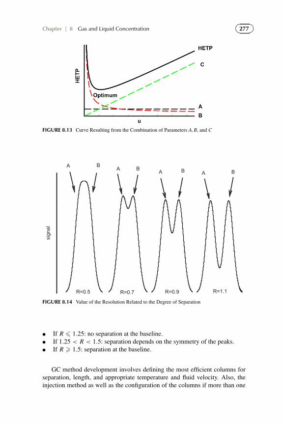
277Chapter | 8 Gas and Liquid Concentration
FIGURE 8.13 Curve Resulting from the Combination of Parameters A,B, and C
sign
al
R=0.5 R=0.7 R=0.9 R=1.1
A A A A BBBB
FIGURE 8.14 Value of the Resolution Related to the Degree of Separation
● If R � 1.25: no separation at the baseline.● If 1.25 < R < 1.5: separation depends on the symmetry of the peaks.● If R � 1.5: separation at the baseline.
GC method development involves defining the most efficient columns forseparation, length, and appropriate temperature and fluid velocity. Also, theinjection method as well as the configuration of the columns if more than one
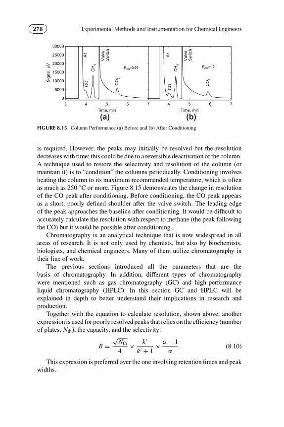
278 Experimental Methods and Instrumentation for Chemical Engineers
FIGURE 8.15 Column Performance (a) Before and (b) After Conditioning
is required. However, the peaks may initially be resolved but the resolutiondecreases with time; this could be due to a reversible deactivation of the column.A technique used to restore the selectivity and resolution of the column (ormaintain it) is to “condition” the columns periodically. Conditioning involvesheating the column to its maximum recommended temperature, which is oftenas much as 250 ◦C or more. Figure 8.15 demonstrates the change in resolutionof the CO peak after conditioning. Before conditioning, the CO peak appearsas a short, poorly defined shoulder after the valve switch. The leading edgeof the peak approaches the baseline after conditioning. It would be difficult toaccurately calculate the resolution with respect to methane (the peak followingthe CO) but it would be possible after conditioning.
Chromatography is an analytical technique that is now widespread in allareas of research. It is not only used by chemists, but also by biochemists,biologists, and chemical engineers. Many of them utilize chromatography intheir line of work.
The previous sections introduced all the parameters that are thebasis of chromatography. In addition, different types of chromatographywere mentioned such as gas chromatography (GC) and high-performanceliquid chromatography (HPLC). In this section GC and HPLC will beexplained in depth to better understand their implications in research andproduction.
Together with the equation to calculate resolution, shown above, anotherexpression is used for poorly resolved peaks that relies on the efficiency (numberof plates, Nth), the capacity, and the selectivity:
R =√
Nth
4× k′
k′ + 1× α − 1
α. (8.10)
This expression is preferred over the one involving retention times and peakwidths.

279Chapter | 8 Gas and Liquid Concentration
FIGURE E8.2 Graphical Analysis of the Complex Mixture
Example 8.2. Based on the chromatogram in Figure E8.2, calculatek′,α,Nth,R, and HETP. The column length is 15 cm × 4.6 mm id.
Solution 8.2. k′:
k′ = tR − t0t0
,
k′A =5.09 min− 1.2 min
1.2 min= 3.24,
k′B =8.03 min− 1.2 min
1.2 min= 5.69.
α:
α = k′Bk′A
, α = 5.69
3.24= 1.76.
Nth:
Nth = 5.54
(tR
W1/2
)2
, Nth = 5.54
(5.09 min
0.14 min
)2
= 7323.
R:
R = 1.177tR2 − tR1
W1,1/2 +W2,1/2, R = 1.177
8.03 min− 5.09 min
0.14 min+ 0.20 min= 10.2.

280 Experimental Methods and Instrumentation for Chemical Engineers
HETP :
HETP = L
Nth, HETP = 15 cm
7323= 0.002 cm.
8.2.9 Gas Chromatography
Gas chromatography is useful in the pharmaceutical, food, environmental, andpetrochemical fields as well as others. It is used for the separation of volatile andsemi-volatile compounds. In gas chromatography, the compounds of interestare in a gaseous state or can be vaporized upon their introduction in the gaschromatograph. The mobile phase is a gas: the most commonly used are helium(He), hydrogen (H2), argon (Ar) and nitrogen (N2). We call the mobile phasethe carrier gas. The choice of carrier gas depends on the detector (detectors willbe discussed later), the separation efficiency, and the speed of analysis.
It is important to set the proper gas pressure or carrier gas velocity for theanalysis. If the gas velocity in the column is too high, the compounds will haveinsufficient time to interact with the stationary phase, which will result in a poorresolution of the peaks. On the other hand, if the carrier gas velocity is too low,the separation will be maximized but the total time to perform the analysis willbe prohibitively long. We need to select an appropriate carrier gas and velocitythat will give the best separation in the least amount of time.
In gas chromatography, the parameters that must be optimized includephysical and chemical properties, such as the temperature and the polarity of themolecule, column parameters and the polarity of the stationary phase. Finally,we must choose a detector and the appropriate injection system.
In capillary GC, the column length varies from 10 m to 100 m with aninternal diameter as little as 1mm. The stationary phase can be liquid or solid.Generally there are three types of GC columns: WCOT (wall-coated opentubular), SCOT (support-coated open tubular), and PLOT (porous-layer opentubular). Figure 8.16 illustrates the three types.
These three column types illustrate possible configurations of the stationaryphase. Together with the column configuration, we also choose the polarity ofthe stationary phase according to the type of molecules to be separated. Fornonpolar compounds (hydrocarbons for example), the type of stationary phasewe can use is a polymer called dimethyl polysiloxane or diphenyl polysiloxane.For compounds with a slight polarity, the type of stationary phase could becyanopropylphenyl dimethyl polysiloxane. For polar compounds, two choicesare possible: polyethylene glycol (often called Carbowax) or biscyanopropyl,cyanopropylphenyl polysiloxane. It is possible to choose the temperature atwhich a mixture of compounds will be analyzed. However, each column willhave a different maximum operating temperature. When possible, it is best touse the column at 30 ◦C below its maximum allowable temperature in order toincrease its lifetime. Using a column at its maximum operating temperature oreven at a higher temperature will cause the column to deteriorate rapidly.

281Chapter | 8 Gas and Liquid Concentration
Support-Coated Open Tubular - SCOT
Wall-Coated Open Tubular - WCOT
Porous-Layer OpenTubular - PLOT
Layer thickness 5-50µm
Internal diameterExternal diameter
Film thickness0.1-8 µm
0.1-0.53µm
FIGURE 8.16 The Three Common Types of Columns for GC
The first compounds detected are often the most volatile as well as thoseof low polarity—the interaction with the stationary phase generally increaseswith polarity. It is often hard to resolve nonpolar peaks efficiently—Ar andN2 is an example—when sampling air; unless specifically considered anddesigned for, the Ar peak will be masked by the nitrogen. (This could introducea systematic error of 1% or more if not accounted for when the nitrogen iscalibrated.) The order in which the compounds appear in the chromatogramis from the most volatile to the least volatile but there are exceptions. Itis also important to consider the nature of the compounds and the type ofstationary phase of the column. Take as an example the 10 compounds inTable 8.2.
It is possible to separate these compounds by GC. But the order in which thecompounds are detected is not from most volatile to least volatile. If a nonpolarcolumn (polydimethyl siloxane) is used, the order will be: 1, 2, 3, 4, 5, 6, 7, 8, 9,and 10.
If we use a column with a different polarity a polyethylene glycol columnfor example, then the order will change to: 2, 5, 8, 10, 1, 4, 7, 3, 6, and 9. So, itis important to be careful with the properties of the stationary phase and thepolarity of the molecules to be separated.
The sample can be injected into the instrument in a liquid or gaseous form.In the case of a gas, we can directly introduce the sample into the column.
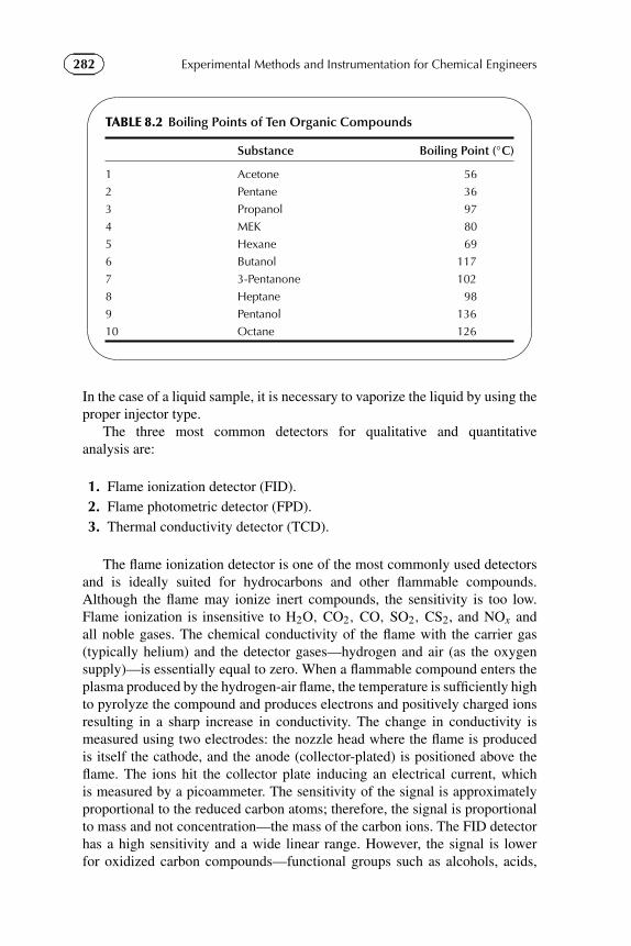
282 Experimental Methods and Instrumentation for Chemical Engineers�
�
�
�
TABLE 8.2 Boiling Points of Ten Organic Compounds
Substance Boiling Point (◦C)
1 Acetone 56
2 Pentane 36
3 Propanol 97
4 MEK 80
5 Hexane 69
6 Butanol 117
7 3-Pentanone 102
8 Heptane 98
9 Pentanol 136
10 Octane 126
In the case of a liquid sample, it is necessary to vaporize the liquid by using theproper injector type.
The three most common detectors for qualitative and quantitativeanalysis are:
1. Flame ionization detector (FID).2. Flame photometric detector (FPD).3. Thermal conductivity detector (TCD).
The flame ionization detector is one of the most commonly used detectorsand is ideally suited for hydrocarbons and other flammable compounds.Although the flame may ionize inert compounds, the sensitivity is too low.Flame ionization is insensitive to H2O, CO2, CO, SO2, CS2, and NOx andall noble gases. The chemical conductivity of the flame with the carrier gas(typically helium) and the detector gases—hydrogen and air (as the oxygensupply)—is essentially equal to zero. When a flammable compound enters theplasma produced by the hydrogen-air flame, the temperature is sufficiently highto pyrolyze the compound and produces electrons and positively charged ionsresulting in a sharp increase in conductivity. The change in conductivity ismeasured using two electrodes: the nozzle head where the flame is producedis itself the cathode, and the anode (collector-plated) is positioned above theflame. The ions hit the collector plate inducing an electrical current, whichis measured by a picoammeter. The sensitivity of the signal is approximatelyproportional to the reduced carbon atoms; therefore, the signal is proportionalto mass and not concentration—the mass of the carbon ions. The FID detectorhas a high sensitivity and a wide linear range. However, the signal is lowerfor oxidized carbon compounds—functional groups such as alcohols, acids,

283Chapter | 8 Gas and Liquid Concentration
carbonyls, amines, halogens, and others: the peak height of ethanol will belower than that of ethane at the same concentration. Another disadvantage ofFID detectors is that the sample is destroyed during its passage through theflame.
Flame photometric detectors are useful to analyze air and water pollutantsand pesticides. It is specific and is mainly used for the analysis of sulfur- andphosphorus-containing compounds. When the effluent gas comes into contactwith the flame, the phosphorus compounds are transformed into HPO and thesulfur compounds to S2. Both HPO and S2 will emit at different wavelengths.Depending on the filter used we will detect either the phosphorus or sulfurcompounds. The light emitted will pass through a photomultiplier and theresulting current is then recorded by a data acquisition system. Dependingon the detector types it can also analyze compounds containing nitrogen andmetals like chrome or tin.
The thermal conductivity detector is a universal detector as it can beapplied to organic and inorganic species. It operates by comparing the electricalconductivity of the effluent from the GC columns with that of a reference gas—the carrier gas. Because of their high thermal conductivity, either helium orhydrogen is used as a carrier gas. The carrier gas passes over an electricallyheated filament made of platinum, tungsten, or nickel and operating at a specifictemperature. Simultaneously, the effluent from the GC column passes overanother electrically heated filament. As the compounds from the GC columnelute, the thermal conductivity of the gas stream decreases, thus changing thethermal conductivity and the resistance of the filament. The lower conductivitycauses the filament temperature to rise since less heat is carried away—hydrogenand helium have very high thermal conductivities compared to other gases.The change in temperature, and thus resistance, is sensed by a Wheatstonebridge circuit resulting in a voltage recorded in µV. Many organic compoundshave a similar thermal conductivity, thus peak areas are comparable and theconcentrations can be estimated by the relative ratios of the peak area. TheTCD is less sensitive than the FID detector and has a lower dynamic range;however, one important advantage is that it is a non-destructive technique sothe effluent may be analyzed with other instruments after the TCD. A massspectrometer may be installed after the TCD—this instrument is referred to asa GC-MS.
8.2.10 High-Performance Liquid Chromatography (HPLC)
Gas chromatography is applicable for compounds with a reasonably highvolatility or molecules that are insensitive to thermal decomposition attemperatures below 200–300 ◦C. HPLC instruments operate in the liquid phaseand are particularly suited for compounds with poor thermal stability or lowvolatility. They may also be used for organic compounds that are volatile. HPLCis very useful for the pharmaceutical and biological industry to separate ionic

284 Experimental Methods and Instrumentation for Chemical Engineers
compounds, polymers, and proteins. In this technique, the mobile phase andthe compounds are liquids. To perform the separation of various compounds,we need to use high-pressure pumps and short columns packed with particlesfrom 3 µm to 7 µm. The particles are silica based with different functionalgroups that allow different column polarities. The resolution increases withdecreasing particle size. The column length varies from 5 cm to 30 cm and hasan internal diameter from 1 mm to 5 mm. Compared to gas chromatography,liquid chromatography will show a lower decrease in efficiency when flow rateis increased. The number of theoretical plates for an HPLC column is calculatedaccording to the following equation:
Nth = 3500 L
dp, (8.11)
where L is the column length in cm and dp is the particle diameter in µm.The number of theoretical plates is proportional to the column length and
inversely proportional to the particle size. The advantage of using small particlesis that they distribute flow more uniformly and, as a result, reduce the eddydiffusion, term A in the Van Deemter equation. However, the smaller particlesincrease the diffusional resistance of the solvent as well as the pressure drop (fora given flow rate). Choosing the flow rate is a critical parameter in developingan HPLC method. Low flow rates allow the analyte sufficient time to interactwith the stationary phase and will affect both the B and C terms of the VanDeemter equation.
Compared with gas chromatography, the mobile phase is a liquid whoseproperties are defined by the analytes. The mobile phase consists of a singlesolvent or solvent mixture to adjust the polarity in order to optimize the analysisconditions.
8.2.11 Method Development
Approaching method development systematically and methodically is criticalto successfully using chromatography. Chromatographs are quite robustwhen maintained properly but frequent maintenance is helpful to minimizeexperimental errors and achieve a high level of productivity. This section isvery important because it outlines a systematic analytical method that can beapplied to other instrumental techniques in chemistry.
First, determine the conditions of the preliminary analysis:
● Type of substance.● Type of column.● Type of detector.● Type of injection.

285Chapter | 8 Gas and Liquid Concentration
After, you must perform the following steps:
1. With the chosen analytical instrument, determine the limit of detection(LOD): the lowest concentration injected into the instrument for which it ispossible to define the presence of a compound in the sample. The signal-to-noise ratio should be greater than about 3. With modern instruments, thiscalculation is performed automatically by the software. Background noise isdefined as the electronic noise of the various components of the instrument.In Figures 8.6 and 8.7, the signal of the highest peak is 5 000 000 µVand the smallest peak is less than 100 000 µV. As long as the noise—the baseline fluctuations as measured in µV—is less than 30 000 µV,the signal is considered significant or quantifiable. The CO peak heightin the chromatogram of Figure 8.15 is at approximately 4000 µV. Thebaseline fluctuations are indiscernible and so the signal-to-noise ratio ismuch greater than 100. Background noise should be minimized to achievethe lowest detection limit, otherwise higher concentrations of the solutesor larger volumes are required. Note that background noise is random andchanges from week to week, from day to day, and even from hour to hour.
2. Determine the quantification limit which is the smallest concentration ofa compound in the sample that gives a detectable signal reproducibly.
3. Calibrate the instrument.Calibration is essential for quantitative results, which relies on generatinga calibration curve using standard solutions of known concentration. Atypical curve will plot the concentration versus the area or height obtained,which is used to determine the linearity of the detector. It is preferableto perform a five-point calibration curve repeated two or three times. Ifnecessary, it can be reduced to three points if the signal is linear in therange of interest.
The limit of linearity is the concentration at which the behavior of thedetector becomes nonlinear—successive increases in concentration resultin a lower than proportional increase in the signal. If the concentrations ofthe samples or standards are too high, then they must be diluted by a factorof between 10 and 1000 or more to achieve a linear detector response. It isimportant to calculate the error on each point and the overall error of thecurve.
4. Perform the analysis of the different samples.When analyzing a series of samples with known concentrations, the orderof analysis should go from the least concentrated to the most concentrated.For unknown samples, a blank test (injection of solvent only) should be runafter each successive sample to ensure that there is no carryover from theprevious injection.
5. Derive the concentration and the analytical error from the calibration curve.6. Document the results.

286 Experimental Methods and Instrumentation for Chemical Engineers
8.3 MASS SPECTROMETRY
Co-author: Patrice PerraultMass spectrometry is a powerful technique to identify atomic masses
of compounds, elemental composition as well as chemical structures. Thecompound is first ionized to generate charged particles. The particles areseparated in an applied electromagnetic field based on their mass-to-chargeratio (m/z) and they are subsequently detected. Ions may be generatedfrom atoms, molecules, clusters, radicals, and/or zwitterions by high energyimpacting electrons formed by an electrically heated filament—electronionization—or by chemical-ion reactions—chemical ionization. Among severalother ionization techniques, inductively coupled plasma—ICP—is commonlyapplied to generate cations. Electrically neutral plasma strips atoms of theirouter electrons after the compound has been atomized by the high temperatures.Chemical ionization is a complex phenomenon in which positive and negativeradical ions can be generated, and in which rearrangements of the resultingradicals can also occur. Ions can also be subject to isomerisation, dissociation,and various other pairings.
Analyte separation follows classical electromagnetic laws. As shown inFigure 8.17, a magnetic field B is applied perpendicularly to a charged particle, q,with an initial velocity, v. The force deflects the moving ions and the magnitudeof the deflection depends on the mass-to-charge ratio.
The major mechanical components of a mass spectrometer (MS) include asample inlet, an ion source, a mass analyser, and a detector. While the sampleinlet is typically open to atmosphere, all other constituents are operated underhigh vacuum (on the order of 10−6 mbar), generated by a turbomolecular pump.The high vacuum is necessary to avoid bimolecular interactions between ions.
The sample inlet is constituted of a heated fused silica capillary, which ismaintained at approximately 200 ◦C and is encased in a flexible tube. Theion source, in the case of electronic ionization, is composed of electricallyheated metallic filaments. Mass analyzers, separating the analytes, include:time-of-flight (TOF), linear quadrupole (Q), linear quadrupole ion trap (LIT),quadrupole ion trap (QIT), Fourier transform ion cyclotron resonance (FT-ICR),etc. These detectors differ in their capacity to treat ion beams in a continuous orpulsed (TOF). Quadrupole mass analyzers stabilize and destabilize the ion pathswith an oscillating electrical field. A “triple quad” is more recent technologyand consists of three quadrupole stages. Quadrupole ion traps will sequentiallyeject ions that have been trapped in a ring electrode between two endcapelectrodes.
MS is used for both quantitative and qualitative analysis (principallyidentification). Figure 8.18 is an analysis of air. The most abundant species isdetected at an amu (atomic mass unit) equal to 28 and its value was 2.87×10⁻⁹,which represents nitrogen. The second most abundant peak is at amu 32 ata value of 0.63 × 10⁻⁹—oxygen. These values are representative of partial

287Chapter | 8 Gas and Liquid Concentration
vq
F = qv B×
FIGURE 8.17 Particle Trajectory Deflection in an Applied Magnetic Field
FIGURE 8.18 Mass Spectrum of Air
pressure (but require a calibration factor). Smaller peaks are recorded at amu40 (argon) and 18 (water) and 44 (CO2). Other peaks that represent fragmentsof molecules or atoms are also evident—amu 14 (nitrogen), amu 16 (oxygen),as well as amu 29, 30, 31, 38, and 39.
Quantitative on-line analysis is difficult without a precise calibrationprocedure. Furthermore, frequent calibration may be required to correct fordrift. Calibration is achieved by analyzing a mixture of a known compositioncomparable to the similar sample of interest from which the instrument’ssensitivity for each compound is evaluated. The sensitivity is a measure ofthe overall response of the instrument for a species when operated underwell-defined conditions. As such, the sensitivity depends on speciesconcentration, as well as on the other analytes’ concentrations. For pure species,the sensitivity is an asymptotic function of the species’ concentration. Processapplications will often use mass spectrometry particularly to monitor gas phasecompositions that are susceptible to the explosion: for selective hydrocarbonoxidation reactions, operating close to the explosion envelope may be desirableto achieve high production rates. Sampling the gas phase at a high frequency(> 2 Hz) can minimize the hazard when the signal is automatically fed to thecontrol system. When the concentration exceeds a threshold value (or evendrops below a value), the interlock will trigger a pre-designated sequence of

288 Experimental Methods and Instrumentation for Chemical Engineers
responses that may include reducing or shutting off the hydrocarbon flow (oroxygen), purging with inert, etc.
Some practical difficulties arise when analyzing mixtures of CO and N2, bothof which have the same amu. The intensity at the amu 28 is a contribution fromboth and differentiating one from the other is difficult. Secondary fragmentsmay be used to quantify CO but it is more convenient, at the experimentalscale, to use argon rather than nitrogen as an inert. For mixtures of compoundsa GC installed upstream is useful such that the MS analyzes one compound ata time and thus overlapping is minimized.
8.4 REFRACTOMETRY
Co-author: Amina BenamerRefractometry is a technique used to detect the concentration of binary
mixtures based on differences in their refractive index. Besides concentration,it is also a simple method to quantify purity. Salinity of brine or sucroseconcentrations in grapes or syrup are two typical applications. Urine-specificgravity is measured for drug diagnostics and plasma protein is assessed byrefractometry in veterinary medicine.
Ernst Abbe first described the technique in 1874. His device consisted ofplacing a sample between two glass prisms. Incident light (monochromatic—typically 589 nm) is introduced from the bottom of the “illuminating prism.” Itpasses through the sample and then is refracted before entering the measuringor refracting prism. When light passes from one object to another (for which thedensities are unequal), it changes direction: the speed of light decreases withincreasing density and this causes it to bend (Klvana et al., 2010, Florentin,2004). The index of refraction, n, is defined as the ratio of the speed of light invacuum, C, to the speed of light in the medium, ν:
n = C/ν.
Figure 8.19 demonstrates the change in angle as an incident ray travelsfrom medium 1, with a refractive index n1, to a denser medium 2 and a higherrefractive index, n2 (Klvana et al., 2010). The beam bends upwards with asmaller angle of incidence closer to the normal of the plane. If medium 1 weredenser than medium 2, the angle of incidence would have been greater and thelight beam would bend away from the normal plane. The relationship betweenthe angle of incidence and of refraction is based on the Snell-Descartes law:
n1 sin θ1 = np sin θp,
where n1 is the refractive index of the medium of interest and n p is the refractiveindex of the prism. Generally, flint glass is chosen as the reference medium(prism) with a refractive index, np, equal to 1.7.

289Chapter | 8 Gas and Liquid Concentration
Incident light
Refracted light
θ1
θ2
Medium 1, n1
Medium 2, n2
FIGURE 8.19 Angle of Incident Light
Prism, np
n1 < np
ilim
Sample, n1
FIGURE 8.20 The Limiting Angle of Refracted Light
For the case in which the incident angle from the sample is at the limit
(θ1 = 90◦), the refracted angle equals arcsin(
n1np
). The operating principle
of refractometers is based on identifying this, as shown in Figure 8.20. Whenlooking through the telescope of a refractometer, the field is divided into tworegions: a darker region, which represents light that is totally reflected and alighter region for which the incidencent light enters at an angle lower than thecritical angle (Figure 8.21). For example, the critical angle of a sugar solutionwith a refractive index of 1.4338 equals 81.7 ◦.
Refractometry is effective for liquids with a refractive index smaller thanthat of flint glass and typically between 1.3 and 1.7. The accuracy is one to twounits to the fourth decimal place.
8.5 SPECTROSCOPY
Co-author: Cristian Neagoe

290 Experimental Methods and Instrumentation for Chemical Engineers
5% 1.440
00%
1.430
FIGURE 8.21 View of Internal Scale and Reflection
8.5.1 Historical
In the seventeenth century, Isaac Newton discovered that light decomposes intothe seven colors of the electromagnetic spectrum—red, orange, yellow, green,blue, indigo, and violet—upon passing through a glass prism. This discoverywas the beginning of spectroscopy. One century later, Joseph Fraunhofer noticedthat light is formed from a great number of spectral lines and he measured thewavelengths of several Fraunhofer lines. Considerable progress occurred in themid-nineteenth century when Foucault observed that the sodium flame emittedby line D also absorbs the radiation D emitted by an electrical arc placed nearby.For the first time, a correlation was made between radiation and the atomicstructure of matter. In 1859, the German physician G. R. Kirchhoff discoveredthat the relationship between emissive power and absorptivity for a fixedwavelength is constant for all bodies at the same temperature. A few years later,Swedish Anders J. Ångström used glass gratings and succeeded in measuringwith very good precision several wavelengths of solar radiation. He introducedthe Ångström unit (1 Å = 10×10−10 m). In 1883, A. A. Michaelson used aninterferometer and measured three Cadmium wavelengths to eight significantfigures. The red cadmium line became a spectrometric standard. By the startof the 20th century, the analytical importance of spectrometric techniques wasclear and the first commercial instruments were manufactured (Williams, 1976).
In spectroscopy, there are two types of spectra: emission spectrum andabsorption spectrum.
8.5.2 Fundamentals
When an atom or molecule is bombarded by thermal, electrical discharge orelectromagnetic radiation, it absorbs energy and enters into an excited state.The atom or molecule returns to its normal state by emitting a spectrum offrequencies of electromagnetic radiation. The emission spectrum is the signatureof each atom and this property is used in industry for qualitative analysis.

291Chapter | 8 Gas and Liquid Concentration
The spectrum is composed of bands of light corresponding to the characteristicwavelengths.
When electromagnetic radiation (light) passes through a transparentmedium, the amount absorbed is a function of the wavelength or frequency.The electromagnetic spectrum of the radiation exiting the medium is composedof dark lines that correspond to the wavelengths absorbed. The emission andabsorption spectra are complementary: the wavelengths in the emission spectracorrespond to the wavelengths absorbed in the absorption spectra.
The information provided by molecular spectroscopy, properly construed,is extremely useful in the qualitative and quantitative research on molecularcomposition. Spectroscopy has the advantage of being very fast and using onlya small amount of material for analysis.
The energy difference between the final state (E f ) and the initial (Ei ) is:
hν = hc
λ= E f − Ei , (8.12)
where h is 6.626 069 57 × 10−34 J s (Planck’s constant), ν is the frequency ofthe radiation emitted or absorbed, λ is the wavelength of the radiation emittedor absorbed, and c is the speed of light.
A molecule can have multiple modes of motion. In this sense, there can bemovements of vibration in which the atomic bond varies in length (longitudinalvibrations) or in which the atoms oscillate in a direction perpendicular to theinteratomic bond (transverse vibrations). Another mode of motion is the rotationof a group of atoms around a node, as shown in Figure 8.22.
The energy absorbed or emitted by the molecules has only quantumfixed values—energy is quantized and is distributed on the energy levelscorresponding to vibrational, rotational, or electronic levels. Electronictransitions occur between two molecular electronic levels. They are usuallyaccompanied by rotational and vibrational transitions.
The principle of spectroscopy is very simple: a sample is exposed to a varyingfrequency of radiation. The outgoing radiation is captured by a detector. Until thefrequency reaches a quantum value, the radiation flux remains constant. Whenthe frequency corresponds to a transition, described by Eq. 8.12, between twoenergy levels, a quantum of energy is absorbed. The absorption results in the
FIGURE 8.22 (a) Vibration Modes in the Molecule of Ethane; (b) Rotation in the Molecule ofEthane

292 Experimental Methods and Instrumentation for Chemical Engineers
detection of the absence of the respective frequency in the outgoing radiationof the sample.
8.5.3 IR Spectroscopy
The spectral range of IR spectroscopy is from 2500 nm to 16000 nm (Hart,2000), which corresponds to the frequency range from 1.9 × 10¹³ Hz to1.2× 1014 Hz. This energy is too small to generate an electronic transition; IRspectra only characterize modes of molecular vibrations. To facilitate readingthe spectra, values are reported as wavenumber, cm−1, which is the reciprocalof wavelength, σ = 1
λ(cm−1).
The main application of IR spectroscopy is the identification of functionalgroups in organic molecules. Other uses are:
1. Determination of the molecular composition of surfaces.2. Identification of chromatographic effluents.3. Determination of molecular conformation (structural isomers) and
stereochemistry (geometric isomers).4. Determination of the molecular orientation in polymers and in solutions.5. Determination of impurities in the test substance.
A great advantage of this method is that it does not destroy the sampleanalyzed. However, there are several limitations:
1. Information on the atomic composition of the molecule is still limited andoften requires the use of complementary analytical techniques as nuclearmagnetic resonance, mass spectroscopy, or Raman spectroscopy.
2. It is important that the solvent does not absorb in the spectral part of themolecule studied.
3. Several molecules are inactive in the infrared spectral part (Sherman Hsu,1997).
The absorption IR spectra are presented in graphical form with thewavelength of the x-axis and the absorption intensity (A) or percenttransmittance (%) on the y-axis. The transmittance is defined as the ratio betweenthe intensity of radiation after passing through the sample (I) and the intensityof the incident radiation (I0):
A = log100
T= − log
I
I0,
Each group of atoms and each bond, whether single, double, or triple,is characterized by a vibrational transition energy. Values are available inseveral public databases ( http://riodb01.ibase.aist.go.jp/sdbs/cgi-bin/direct_frame_top.cgi, http://webbook.nist.gov/chemistry/vib-ser.html, http://www.ir-spectra.com/indexes/index_d.htm) and some of them are given in Table 8.3.
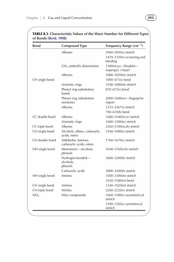
293Chapter | 8 Gas and Liquid Concentration�
�
�
�
TABLE 8.3 Characteristic Values of the Wave Number for Different Typesof Bonds (Byrd, 1998)
Bond Compound Type Frequency Range (cm−1)
Alkanes 2960–2850(s) stretch
1470–1350(v) scissoring andbending
CH3 umbrella deformation 1380(m,w)—Doublet—isopropyl, t -butyl
Alkenes 3080–3020(m) stretch
CH single bond 1000–675(s) bend
Aromatic rings 3100–3000(m) stretch
Phenyl ring substitutionbands
870–675(s) bend
Phenyl ring substitutionovertones
2000–1600(w)—fingerprintregion
Alkynes 3333–3267(s) stretch
700–610(b) bend
CC double bond Alkenes 1680–1640(m,w) stretch
Aromatic rings 1600–1500(w) stretch
CC triple bond Alkynes 2260–2100(w,sh) stretch
CO single bond Alcohols, ethers, carboxylicacids, esters
1260–1000(s) stretch
CO double bond Aldehydes, ketones,carboxylic acids, esters
1760–1670(s) stretch
OH single bond Monomeric—alcohols,phenols
3640–3160(s,br) stretch
Hydrogen-bonded—alcohols,phenols
3600–3200(b) stretch
Carboxylic acids 3000–2500(b) stretch
NH single bond Amines 3500–3300(m) stretch
1650–1580(m) bend
CN single bond Amines 1340–1020(m) stretch
CN triple bond Nitriles 2260–2220(v) stretch
NO2 Nitro compounds 1660–1500(s) asymmetricalstretch
1390–1260(s) symmetricalstretch

294 Experimental Methods and Instrumentation for Chemical Engineers
FIGURE 8.23 IR Spectrum of Lactic Acid (SDBSWeb, retrieved 2012)
�
�
�
�
TABLE 8.4 Wave Numbers and Bonds
Wave Number (cm−1) Assigned Group
3410 OH single bond (alcohol)
2990, 2943 CH single bond stretch
2633 OH single bond stretch in carboxylic acids
1732 CO double bond stretch in carboxylic acids
1456 Umbrella effect in methyl, bending
1376 OH single bond bending in carboxyl group
1220 CO single bond stretch in CHO group
747 CO single bond bending in CHO group
Figure 8.23 is an example of a resolved IR spectrum of the lactic acidmolecule. The data wave number and associated bonds are given in Table 8.4.
8.5.4 Spectroscopy UV/Visible
The spectral range corresponding to the spectroscopic UV/Visible is from100 nm to 800 nm, but a narrower interval is more common from 190 nmto 750 nm. The UV range lies between 190 nm and 380 nm and the visiblecomponent is from 380 nm to 750 nm. The energy in this spectral range isgreater than that of the IR range and generates electronic transitions in additionto vibrational and rotational transitions. The distances between the rotationallevels are smaller than those between vibrational levels while the higher energiesare found in electronic transitions. Electronic transitions are accompanied by
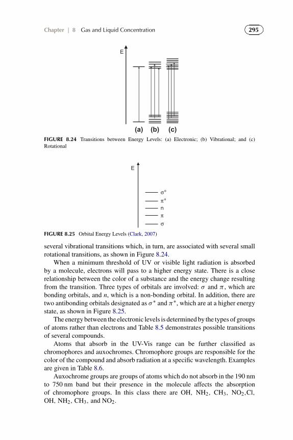
295Chapter | 8 Gas and Liquid Concentration
E
(a) (b) (c)FIGURE 8.24 Transitions between Energy Levels: (a) Electronic; (b) Vibrational; and (c)Rotational
n
σ
σ∗
π
π∗
E
FIGURE 8.25 Orbital Energy Levels (Clark, 2007)
several vibrational transitions which, in turn, are associated with several smallrotational transitions, as shown in Figure 8.24.
When a minimum threshold of UV or visible light radiation is absorbedby a molecule, electrons will pass to a higher energy state. There is a closerelationship between the color of a substance and the energy change resultingfrom the transition. Three types of orbitals are involved: σ and π , which arebonding orbitals, and n, which is a non-bonding orbital. In addition, there aretwo antibonding orbitals designated as σ ∗ and π∗, which are at a higher energystate, as shown in Figure 8.25.
The energy between the electronic levels is determined by the types of groupsof atoms rather than electrons and Table 8.5 demonstrates possible transitionsof several compounds.
Atoms that absorb in the UV-Vis range can be further classified aschromophores and auxochromes. Chromophore groups are responsible for thecolor of the compound and absorb radiation at a specific wavelength. Examplesare given in Table 8.6.
Auxochrome groups are groups of atoms which do not absorb in the 190 nmto 750 nm band but their presence in the molecule affects the absorptionof chromophore groups. In this class there are OH, NH2, CH3, NO2,Cl,OH, NH2, CH3, and NO2.

296 Experimental Methods and Instrumentation for Chemical Engineers�
�
�
�
TABLE 8.5 Electronic Transitions and λmax for Various Substances
Compound Transition λmax (nm)
Ethane σ → σ∗ 135
Methanol σ → σ∗ 150
n→ σ∗ 183
Ethylene π → π∗ 175
Benzene π → π∗ 254
Acetone n→ π∗ 290
�
�
�
�
TABLE 8.6 Characteristic Wavelengths of the Principal Chromo-phore Groups (Tables of Physical & Chemical Constants, 2005)
Group Formula λmax (nm)
Nitrile −CN < 180
Ethylene −C = C− < 180
Sulphone −SO2− 180
Ether −O− 185
Ethene −C = C− 190
Thiol −SH 195
Amine −NH2 195
Bromide −Br 210
Iodide −I 260
Ketone > C = O 195, 275
Nitro −NO2 210
Nitrite −O−NO 225
Nitrate −O−NO2 270
Azo −N = N− > 290
Nitroso −N = O 300
The type of solvent used in the analysis may influence the absorption. In thecase of a nonpolar substance in a nonpolar solvent, the influence of the solventis negligible but in the case of polar molecules in polar solvents, there are fairlystrong solute-solvent interactions, which usually lead to a decrease in resolutionof the spectrum.
One of the most widespread applications in industry of the UV-Visspectroscopy is the determination of the concentration of solutions. A wavepassing through a transparent medium, a solution, for example, loses some

297Chapter | 8 Gas and Liquid Concentration
of its energy. The Lambert-Beer law correlates intensity of absorbed incidentradiation and the concentration of the solution. The energy absorbed, absorbance(A), or transmitted, transmittance (T), follows a logarithmic function of theabsorption coefficient, ε, concentration, C, and the path length, l:
A = logI0
I= log
100
T= εCl.
UV-visible spectroscopy is used for quantitative analysis, studies ofreaction rate and mixtures, identifying compounds and as detectors for HPLC.Quantitative analysis requires calibration curves to adequately characterize thevariation of concentration and absorbance (or transmittance). Reaction ratesmay be derived by following the variation of the concentration of a compoundin a vessel with time-on-stream. The total absorbance is the sum of the individualabsorbances.
Spectroscopy has the advantage of being non-destructive and it is availableat an affordable price. It can also be used for a wide variety of substances withgood precision, sensitivity, and short analysis time. One major limitation is thatthe spectra are difficult to interpret for mixtures.
8.6 X-RAYS
Co-author: Amina BenamerWilhelm Conrad Röntgen discovered X-rays on the night of November 8, 1895while he was conducting tests on cathode rays with Crookes tubes (Demerdijian,2007). The “X” represents an unknown as was taken from algebra where itrepresents an unknown variable. This discovery earned him a Nobel Prize inphysics in 1901. In December 1895, he produced an image of his wife’s handwith an X-ray. As shown in Figure 8.26, it clearly shows bones as well as herwedding ring (Bellis, 2012).
FIGURE 8.26 First X-ray Image, 1895

298 Experimental Methods and Instrumentation for Chemical Engineers
X-rays have different characteristics and unique properties, such as beingable to traverse many transparent and opaque materials such as glass, tissue, andsome metals, including lead. These rays are invisible and propagate in vacuumat the speed of light in a straight line.
This astounding discovery is widely used today and has taken an importantplace in society. Indeed, X-rays are now used in medicine to detect abnormalitiesin the human body (radiography, CT, etc.). X-rays are also used to remove cancercells. Obviously, this practice can also be harmful to healthy cells if it is notused prudently. Also at airports, baggage is scanned by X-ray to identify liquidsare other potentially hazardous objects.
Both X-ray fluorescence and X-ray diffraction are techniques used forchemical analysis. In X-ray fluorescence, gamma rays and high energy X-raysbombard a sample and secondary/fluorescent rays are emitted and detected.In X-ray diffraction, a X-ray beam is focused on a sample at various angles.The scattered intensity of the beam is detected. The nature of the scatter—refracted—beam reveals the crystal structure, chemical composition, and otherphysical properties.
8.7 EXERCISES
8.1 Para-nitrochlorobenzene (PNCB—C6H4ClNO2) is an important inter-mediate and is used as an antioxidant in rubber. Parameters derived froma GC chromatogram of three compounds withdrawn from a reactor—chlorobenzene (C6H5Cl), toluene (C6H5CH3), and PNCB—are shownin Table Q8.1. The GC column was 55 cm long. M. Abdul-Halem
(a) Calculate the number of theoretical plates for chlorobenzene.(b) What is the height of an equivalent theoretical plate for
chlorobenzene?(c) What is the resolution between PNCB and toluene?(d) How many theoretical plates are required to achieve a resolution of
1.8 for chlorobenzene and PNCB?(e) What would the new column’s length be?
�
�
�
�
TABLE Q8.1 GC Analysis
Compound tR (min) w1/2 (s)
Reference 1.00 -
Chlorobenzene 7.00 34.2
PNCB 8.175 36.9
Toluene 10.05 47.7

299Chapter | 8 Gas and Liquid Concentration
8.2 The chromatogram for a two-component mixture was separated on a20 cm × 55 mm ID column. The reference peak was detected at 2 minand the retention time of the 2 compounds was 4 min and 8 min. Themaximum peak heights of each peak are 50 mV (4 min) and 20 mV(8 min). Determine: A. M. Bélanger
(a) The capacity factor.(b) The selectivity factor.(c) The number of theoretical plates.(d) The resolution.(e) The equivalent height of a theoretical plate.
8.3 Natural gas is composed primarily of methane but may contain otherhydrocarbons (ethane, propane, etc.), hydrogen sulfide, mercury, carbondioxide, water, and nitrogen. C. Mathieu
(a) Five sample Hoke cylinders (originally containing air) were chargedwith shale. Complete the missing parameters in Table Q8.3.
(b) Among the components of the raw natural gas, some of them mustbe removed for reasons of safety, environmental hazards, and riskof corrosion in treatment facilities or during transportation. The gasis analyzed after a desulfurization step with a non-dispersive IRanalyzer to evaluate the effectiveness of the desulfurization processinstalled:
(i) Determine the concentration of sulfur remaining in the naturalgas stream coming out of the desulfurization unit.
(ii) If the maximum allowable concentration of H2S in pipelines is4 ppmv. Is the desulfurization unit efficient?
Note that ε = 4.2062 × 10³ l mol−1 cm−1 for H2S. The opticalreference path is b0 = 50 cm, the optical path of the sample is
�
�
�
�
TABLE Q8.3 Sample Data for Natural Gas Analysis
Exp Sample Volume Flow Rate Sampling Time Ratio c/ci
(ml) (ml min−1) (min)
1 3250 285 ? 0.99
2 ? 230 40 0.96
3 3300 ? 55 0.975
4 3000 200 60 ?

300 Experimental Methods and Instrumentation for Chemical Engineers
b = 29.5 cm. The concentration of reference natural gas in the analyzeris c0 = 15 mg m−3, and the conversion factor for the H2S is 1 mg
1 l air =717 ppm (at 25 ◦C and 760 mmHg).
8.4 Parameters of a chromatogram to quantify the concentration of oxygenin air are: t0 = 0.6 min, tR,O2 = 2.0 min, tR,N2 = 3.2 min. S. Mestiri
(a) Calculate the capacity factor of the first peak.(b) Does changing the carrier gas change k′? Why?(c) Calculate the selectivity. Are the two peaks well separated?(d) Calculate the resolution knowing that wO2 ,1/2 = 0.1 min and wN2 ,
1/2 = 0.3 min.(e) Are the peaks well resolved?
8.5 The concentration of iodine in solution is measured by UV/Visspectrophotometry. The absorbance of the solution A equals 0.5 andε(λ) = 250. N. Paulin
(a) Using the Beer-Lambert law, find the iodine concentration in thesample.
(b) What would be the concentration of iodine if the readout for thetransmittance was 56%?
Note that the cell used is cylindrical and has a volume capacity of4 cm and V = 5× 10⁻⁶ m3.
8.6 Hydrazine reacts with benzaldehyde to form benzalazine. A chroma-togram based on a HPLC analysis is shown in Figure Q8.6. V. MessierThe column is 250 mm× 4.6 mm, phase KROMASIL 5 µm, the mobilephase is acetonitrile/acidified water 0.01%H2SO4 80/20, the flow rate is1.5 ml mm−1, the volume injected is 25 µl, and the UV wavelength is313 nm.
FIGURE Q8.6 Chromatogram of the Sample Collected During the Reaction
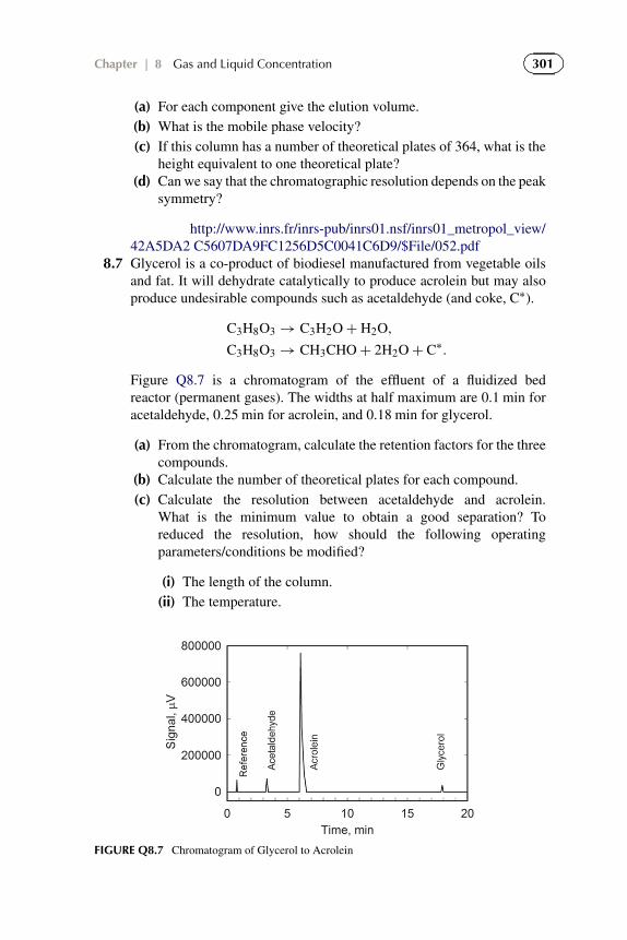
301Chapter | 8 Gas and Liquid Concentration
(a) For each component give the elution volume.(b) What is the mobile phase velocity?(c) If this column has a number of theoretical plates of 364, what is the
height equivalent to one theoretical plate?(d) Can we say that the chromatographic resolution depends on the peak
symmetry?
http://www.inrs.fr/inrs-pub/inrs01.nsf/inrs01_metropol_view/42A5DA2 C5607DA9FC1256D5C0041C6D9/$File/052.pdf
8.7 Glycerol is a co-product of biodiesel manufactured from vegetable oilsand fat. It will dehydrate catalytically to produce acrolein but may alsoproduce undesirable compounds such as acetaldehyde (and coke, C∗).
C3H8O3 → C3H2O+ H2O,
C3H8O3 → CH3CHO+ 2H2O+ C∗.
Figure Q8.7 is a chromatogram of the effluent of a fluidized bedreactor (permanent gases). The widths at half maximum are 0.1 min foracetaldehyde, 0.25 min for acrolein, and 0.18 min for glycerol.
(a) From the chromatogram, calculate the retention factors for the threecompounds.
(b) Calculate the number of theoretical plates for each compound.(c) Calculate the resolution between acetaldehyde and acrolein.
What is the minimum value to obtain a good separation? Toreduced the resolution, how should the following operatingparameters/conditions be modified?
(i) The length of the column.(ii) The temperature.
FIGURE Q8.7 Chromatogram of Glycerol to Acrolein

302 Experimental Methods and Instrumentation for Chemical Engineers
(iii) The linear velocity of the mobile phase.(iv) The amount of stationary phase.
(d) The selectivity of the acrolein is calculated from the followingequation:
S = [Cacrolein][Cacrolein] + [Cacetaldehyde] .
What is the uncertainty of selectivity for the following data (in µV, α
concentration): for acrolein, 835 000, 825 000, 845 000, and 815 000;for acetaldehyde, 50 000, 80 000, 95 000 and 95 000, and xacr =830 000,sacr = 13 000,xace = 80 000,sace = 21 000.
8.8 A gas chromatograph is used to examine the concentration of toxicchemicals from shale gas. The following compounds are suspected tobe present with the methane: benzene, methylbenzene, parabenzene, andhydrogen sulfide.
(a) Which of the following three detectors would be appropriate for theanalysis?
(i) FID (flame ionization detector).(ii) TCD (thermal conductivity detector).(iii) FPD (flame photometric detector).
(b) Figure Q8.8 is a chromatogram in which the peaks appear in orderof increasing molecular weight. The reference peak appears at 55 s.
(i) What is the retention factor of each pollutant?
FIGURE Q8.8 Initial Analysis with Standards

303Chapter | 8 Gas and Liquid Concentration
(ii) What is the selectivity factor between hydrogen sulfide andparabenzene?
(iii) What is the resolution factor between benzene andmethylbenzene?
(iv) Is the resolution sufficient?(v) Identify two ways to increase the resolution between these two
pollutants?
8.9 (a) What is the advantage of using a gas chromatograph with atemperature program?
(b) Why do we use hydrogen or helium as a mobile phase?(c) Give three examples of solute that can be detected with the FID and
three examples of non-detectable solutes.(d) You measure the hydrocarbon concentration in a gas stream
containing three solutes, including heptane and decane. Theretention times of heptane and decane are respectively of 14.5 minand 22 min. The unknown solute leaves after 19 min. The residencetime of tracer gas (non-retained) is 1 min. The peak widths at half-height of the solutes are 1.1 min for heptane, 1.4 min for decane, and1.7 min for the unknown solute.
(i) If the unknown gas is an alkane, how many carbons could ithave?
(ii) Calculate the capacity factor for each hydrocarbon.(iii) Calculate the separation factor for both heptane and decane with
respect to the unknown.(iv) What are the parameters of resolution of heptane and decane
with respect to the unknown? Are the peaks well resolved(separated)?
8.10 At the neolithic site of Kovacevo, Bulgaria, archeologists found severalceramic vases from 6200 to 5500 BC. For more than 20 yr, a debatehas raged over the utility of these vases. A sample of black materialwas taken from inside one of the vases to determine its composition.An infrared spectrometric analysis (IRTF) was performed to determinethe presence of organic material. To then identify the principal organicconstituents, gas chromatography was used. The resulting chromatogramis shown in Figure Q8.10. The length of the column is 15 m and T0 is660 s. Table Q8.10 shows more data. A. Bérard
(a) Find the four constituents of the peaks of the black powder sampleof vase KOV G264 1T. For ceramides, k′ = 2.08, for cholesterol,the capacity factor is 0.995, for fatty acids, Nth = 18754, forglycerolipids, HETP = 0.009 cm, for triglycerine, the separationfactor is 1.02, and for diglycerine, R = 2.12.

304 Experimental Methods and Instrumentation for Chemical Engineers
FIGURE Q8.10 Kovacevo Vase Chromatogram: (Vieugué et al., 2008)
�
�
�
�
TABLE Q8.10 Data for Kovacevo Vase Chromatogram
Peak W1/2 (s)Fatty Acids 4, 6, 13, 12, and 10
Cholesterol 8
Diglycerides 16 and 14
Triglycerides 4, 7, 5
(b) What is the effect on the velocity of the mobile phase if the columnlength is decreased?
(c) Calculate the uncertainty in the resolution of diglyceride peakknowing that the uncertainty of the retention time is 0.1 min andthat of W1/2 is 1 s.
(d) Several samples of black powder were analyzed by chromatography.The internal standard was observed at several different times (inmin): 21.3, 22.0, 24.2, 23.8, 20.4, 21.7, and 25.1. Can the internalstandard peak, shown in Figure Q8.10, be considered as the internalstandard (use the Chauvenet criterion).
8.11 Two peaks of a chromatogram appear near 7.5 min. Other conditionsrecorded were: t0 = 3 min,W1/2 = 0.35 min, HEPT = 0.005 cm, andthe selectivity is 0.98.

305Chapter | 8 Gas and Liquid Concentration
(a) Calculate the number of theoretical plates. Determine the efficiencyfactor as well as the length of the column.
(b) Calculate the capacity factor.(c) Calculate the resolution. What can you determine from this?
8.12 The chromatogram of a 17 cm × 4 mm column contains peaks att0 = 0.3 min, tR,1 = 1.6 min, and tR,2 = 1.8 min. In addition,W1,1/2 = 0.1 min and W2,1/2 = 0.08 min.
(a) Find the separation factor α (selectivity).(b) What is the resolution?(c) Find the number of theoretical plates.(d) Determine the equivalent height of a theoretical plate.(e) What is the effect of increasing the temperature of the column on
the retention time?(f) What is the effect of increasing the flow rate of the mobile phase on
the retention time?
8.13 For each peak shown in Figure Q8.13, identify the correspondingcompound and the bond.
wavenumber, cm-101000200030004000
abso
rban
ce
0.0
0.2
0.4
0.6
0.8
1.0
1
1
1
23
3
1 - CO2 - CO23 - Ethane
FIGURE Q8.13 IR Spectra
REFERENCES
Bellis, M., n.d. History of the X Ray. Retrieved July 2012, from About.com—Inventors: <http://inventors.about.com/od/xyzstartinventions/a/x-ray.htm>.
Byrd, J., 1998. Interpretation of Infrared Spectra, 1998. Retrieved July 20, 2012 from:<http://wwwchem.csustan.edu/tutorials/infrared.htm>.
306 Experimental Methods and Instrumentation for Chemical Engineers
Clark, J., 2007. UV-Visible Absorption Spectra. Retrieved July 2012, from UV-Visible: <http://www.chemguide.co.uk/analysis/uvvisible/theory.html>.
Demirdjian, H., 2007, October 10. La radiographie (I)—Histoire de la découverte des rayonsX et de leur application en médecine. Retrieved July 2012, from Rayons X: <http://culturesciences.chimie.ens.fr/content/la-radiographie-i-histoire-de-la-decouverte-des-rayons-x-et-de-leur-application-en-medecine-1196>.
Florentin, E., 2004, May 10. Le réfractomètre. Retrieved July 2012, from ENS de Lyon-éduscol:<http://culturesciencesphysique.ens-lyon.fr/XML/db/csphysique/metadata/LOM_CSP_Refrac-tometre.xml>.
Hart, H., Conia, J.-M., 2000. Introduction à la chimie organique. Dunod, Paris.Klvana, D., Farand, P., Poliquin, P.-O., 2010. Méthodes expérimentales et instrumentation—Cahier
de laboratoire. École Polytechinique de Montréal, Montréal.Kaye, G.W.C., Laby, T.H., 1911. Tables of Physical Constants and some Mathematical Functions,
Longmans, Green and Co., New York. Tables of Physical & Chemical Constants (16thedition 1995). 3.8.7 UV-Visible Spectroscopy. Kaye & Laby Online. Version 1.0 (2005)www.kayelaby.npl.co.uk.
Patience, G.S., Hamdine, M., Senécal, K., Detuncq, B., 2011. Méthodes Expérimentales EtInstrumentation En génie Chimique, third ed. Department Chemical Engineering, EcolePolytechnique de Montreal.
SDBSWeb. <http://riodb01.ibase.aist.go.jp/sdbs/>. National Institute of Advanced IndustrialScience and Technology. Retrieved July 20, 2012.
Sherman Hsu, C.-P., 1997. Infrared spectroscopy. In: Settle, Frank (Ed.), Handbook of InstrumentalTechniques for Analytical Chemistry. Retrieved July 20, 2012 from:<http://www.prenhall.com/settle/chapters/ch15.pdf>.
Vieugué, J., Mirabaud, S., Regert, M., 2008. Contribution méthodologique á l’analyse fonctionnelledes céramiques d’un habitat néolithique: l’exemple de Kovacevo (6 200-5 500 av. J.-C., Bulgarie),ArcheoSciences, 32, 99–113.
Williams, Dudley, 1976. Spectroscopy. Methods in Experimental Physics, vol. 13. Academic PressInc., New York.

Chapter 9
Analysis of Solids and Powders
9.1 OVERVIEW
Particle technology and the analysis of solids involve the measurement of phys-ical properties, the assessment of the impact of these properties on operations,and the identification of means to improve, develop, and design processes.Powder systems touch many chemical industries, and the majority of consumerproducts necessarily pass through the manipulation of particulates in their man-ufacturing process. The analysis and characterization of multi-phase systemsnot only includes gas-solids and liquid-solids systems but also two phase liquidsystems, three phase systems, gas-liquids as well as micron-sized powders andnano-particles. Besides the chemical industry, other industries in which particletechnology plays an important role include the pharmaceutical (pills, colloids,solutions, suspensions), agricultural (distribution of pesticides, herbicides, fer-tilizers, soil), food (flour, sugar, Cheerios, salt, etc.), construction (cement, con-crete, asphalt), power industry (coal), mining, metallurgy, and the environment.
The combustion of coal to produce electricity is the greatest contributor togreenhouse gases and the manufacture of cement is third accounting for as muchas 5% of the global CO2. Concrete and asphalt are the two largest manufacturedproducts and both are aggregates of particles. Annual production of concrete isapproximately 2 × 10⁹ kt yr−1 while the production of cement is on the orderof 2 × 10⁹ kt yr−1 (van Oss, 2011).
Cement manufacture is illustrative of unit operations involving solids—conveying (transport), grinding—milling—crushing (micronization), sieving(separation), and reaction. Mined limestone from a quarry passes through aprimary jaw crusher (communition or grinding). The ore enters a vibratingscreen to separate the ore into three fractions: particles greater than 120 µm indiameter are conveyed by a belt conveyer to a secondary crusher and then to
Experimental Methods and Instrumentation for Chemical Engineers. http://dx.doi.org/10.1016/B978-0-444-53804-8.00009-5© 2013 Elsevier B.V. All rights reserved. 307

308 Experimental Methods and Instrumentation for Chemical Engineers
a hammer mill so that all the ore is less than 120 µm; particles from 50 µmto 120 µm are screened. After a secondary screening, particles are separatedinto three fractions—0–25 µm, 25–50 µm, and 50–120 µm and stockpiled inopen pits. The next step is to micronize the particles to a fine powder less than125 µm. This powder is fed to a rotary kiln in which the powder temperaturereaches 1450 ◦C and the flame temperature reaches 2200 ◦C. Calcium carbonate(limestone) is calcined to produce lime and CO2:
CaCO3 → CaO + CO2.
In this step, 40% of the CO2 is due to fossil fuel combustion to produce theflame, and 50% comes from the reaction. Because of the high temperatures,the powder agglomerates (forms clinkers). Before packaging and distribution,these particles are milled and sieved to the desired size.
Besides the processing steps mentioned for cement manufacture, other unitoperations involving solids include: filtration, cyclonic separation, decantation(sedimentation), coating (polymer coatings of metals, for example), pneumaticconveying (of flour, grain, coal, alumina), crystallization (manufacture ofcatalysts and foodstuffs), mixing (pharmaceuticals—ensuring the activeingredient is uniformly distributed before making pills), drying, etc. In thischapter, we focus primarily on the physical characteristics of powders andsolids—density, shape, and particle size.
9.2 DENSITY
The densities of gases are readily calculated through thermodynamicrelationships and liquid densities are straightforward to measure compared tomeasuring solids and powder densities. Table 9.1 summarizes densities ofmany solids; they range from as low as 100 kg m−3 for nano-tubes to almost20 000 kg m−3 for tungsten. There is a significant variation between differenttypes of wood. The highest density woods are lignum vitae (1370 kg m−3) andebony (1120 kg m−3), while the lowest include balsa (170 kg m−3), bamboo(300 kg m−3), and red cedar (380 kg m−3). The average density is 600 kg m−3
with a standard deviation of 200 kg m−3 (The Engineering Tool Box, retrieved2011).
9.2.1 Bulk Density
Powders are characterized by three different measures of density: skeletaldensity, particle density, and bulk density. Bulk density, ρb, is the density ofthe powder that is typically packaged in a container (sack, box, silo, vessel).However, it generally increases with time and thus two other measures areoften quoted to characterize the bulk density: pour density and tapped density.During shipping, or as the powder is moved from one place to another, the

309Chapter | 9 Analysis of Solids and Powders�
�
�
�
TABLE 9.1 Densities of Typical Solids and Powders
Solid Density (kg m−3)
Nano-tubes 100
Acrylic fibers 144
Colorant 144
Polypropylene 481
PVC chips 513
Coal dust 561
Wood 600 ± 200
Alumina 641
Polyethylene 689
Clay 802
Ice 917
Cerium oxide 994
Cement 1363
Phosphates 1443
FCC catalyst 1507
Sand 2651
Zinc powder 3367
Tungsten carbide 4008
Steel 7850
Tungsten 19 250
powder becomes more compacted. The pour density represents the lowest levelof compaction—the conditions immediately after the powder is introduced intoa container—this is the value generally reported as the “bulk” density. Thehighest level of compaction is referred to as the tapped density. The two aremeasured by first pouring the powder into a graduated cylinder to a certainheight, hb, (from which ρb is calculated) and then the cylinder is tapped gentlyon the side with a ruler until the solids level no longer drops, ht . The ratio ofthe tapped density to the bulk density is referred to as the Hausner ratio:
H = ρt
ρb= hb
ht. (9.1)
The Hausner ratio is a parameter that indicates how much a powdermight compact with time, which correlates with how it will flow—flowability.Values greater than 1.25 indicate that the powder will have poor flowabilitycharacteristics. The Scott density is the standard test to measure bulk densityor poured density.

310 Experimental Methods and Instrumentation for Chemical Engineers
FIGURE E9.1 Scott Density Measurement Apparatus
Example 9.1. The Scott density is measured using a standardized procedurein an apparatus shown in Figure E9.1. The powder is fed to a funnel at the topof the device and it falls through a series of baffles in a chute that redirect theflow and finally into a hollow cylinder (or cube) with a 1 cm3 volume. When thecylinder at the bottom overflows, it is removed from underneath the chute andexcess powder is leveled with a spatula (or ruler). The weight of the powder (g)divided by 1 cm3 gives the Scott density—which is equivalent to bulk density.
Example 9.1. Three students measured the mass of three powders—sand,fluid catalytic cracking catalyst (FCC), and Ca3(PO4)2—10 times successivelyin a Scott Volumeter. The data is summarized in Table E9.1. Calculate theScott density, uncertainty, and repeatability. The volume and uncertainty of thecylinder is 25.00 ± 0.03 cm3.
Solution 9.1. The mean mass of catalyst, mcat, collected, standard deviationand the uncertainty,�cat, are first calculated. (Note that the uncertainty is definedas the 95% confidence interval and, in this case it is quite close to the standarddeviation.)
Since the uncertainty of the volume of the cylinder is less than five timesthe uncertainty in the mass of powder, it may be ignored. The uncertainty in thedensity is simply:
�ρ = �mcat
mcatρ.

311Chapter | 9 Analysis of Solids and Powders�
�
�
�
TABLE E9.1 Mass of Powder Collected by Three Students in ScottVolumeter
Sand
1 37.93 38.20 38.10 38.38 38.31 38.62 38.50 38.10 38.31 38.00
2 38.26 38.09 37.72 38.03 38.34 38.64 38.12 37.96 38.71 38.28
3 38.33 38.15 38.35 38.21 38.24 38.03 38.07 37.53 38.23 38.01
FCC
1 21.04 21.02 21.00 20.88 20.98 21.23 21.07 21.15 21.07 21.30
2 21.37 22.00 21.41 21.08 21.34 20.97 22.02 21.88 22.33 21.42
3 22.74 22.33 22.41 22.81 22.26 22.59 22.37 22.46 22.78 22.95
Ca3(PO4)21 8.11 7.99 7.91 7.97 7.98 7.93 7.90 8.07 7.89 7.87
2 8.24 8.00 7.98 8.23 7.98 8.07 7.86 7.74 8.24 7.95
3 8.03 7.86 8.15 8.09 7.94 7.96 7.89 7.95 7.83 7.97
�
�
�
�
TABLE E9.1Sa Mean Mass and Statistics for the Scott Density Measuredfor Each Powder
Sand FCC Ca3(PO4)2
Student 1 2 3 1 2 3 1 2 3
Mean mass 38.25 38.22 38.12 21.07 21.58 22.57 7.96 8.03 7.97
Standard deviation (s) 0.22 0.30 0.24 0.12 0.45 0.24 0.08 0.17 0.10
�m 0.16 0.22 0.17 0.09 0.32 0.17 0.06 0.12 0.07
The agreement between the mean values of the students for the sand isbetter than for either the FCC or the calcium phosphate. The particle size wasmuch larger for the sand and it was less cohesive. The repeatability variance, asdescribed in Chapter 2, equals the sum of the variances of each sample dividedby the number of samples subtracted by 1 (see Tables E9.1Sa and E9.1Sb):
s2r = 1
n − 1
∑s2r ,i .
The repeatability variance and standard deviation for the Scott density ofeach sample are shown in Table E9.1Sc.
If the samples were run in different laboratories, the reproducibility is(Table E9.1Sd):
s2R = s2
L + s2r .

312 Experimental Methods and Instrumentation for Chemical Engineers�
�
�
�
TABLE E9.1Sb Scott Density and Uncertainty Measured for Each Powder
Sand FCC Ca3(PO4)2
Student 1 2 3 1 2 3 1 2 3
ρ 1.530 1.53 1.52 0.8430 0.8633 0.903 0.318 0.321 0.319
Standard 0.009 0.01 0.01 0.005 0.02 0.009 0.003 0.007 0.004
deviation (s)
�ρ 0.006 0.009 0.007 0.004 0.01 0.007 0.002 0.005 0.003
%�ρ 0.4 0.6 0.4 0.4 1.5 0.8 0.7 1.5 0.9
�
�
�
�
TABLE E9.1Sc Repeatability Variance and Standard Deviation for the ScottDensity
s2r sr (g cm−3)
Sand 0.007 0.09
FCC 0.008 0.09
Ca3(PO4)2 0.003 0.06
�
�
�
�
TABLE E9.1Sd Scott Density Reproducibility
s2R sR (g cm−3)
Sand 0.014 0.12
FCC 0.032 0.18
Ca3(PO4)2 0.007 0.08
9.2.2 Particle Density
The particle density, ρb, represents the mass of a particle divided by the volumeof its hydrodynamic envelope. It includes the void spaces of open pores thatcommunicate with surrounding fluid but also internal pores:
ρp = m p
Vp. (9.2)
As shown in Figure 9.1, the hydrodynamic envelope for a spherical particleis equal to the volume of the sphere. Most particles are non-spherical in shape

313Chapter | 9 Analysis of Solids and Powders
OpenPores
ClosedPores
HydrodynamicEnvelope
FIGURE 9.1 Particle Density
and thus defining the hydrodynamic envelope is problematic. Typically, theparticle density is measured using pycnometry or by mercury porosimetry.
Either a graduated flask or a high precision pycnometer may be used toestimate the particle density, but these techniques are poor measures whenthe solids are soluble. Therefore, a liquid should be chosen for which thesolids are insoluble. The test should be conducted rapidly to minimize eitherdissolution of the solids are the partial filling of open pores. To increase theprecision, the graduated flask or pycnometer should first be calibrated with thefluid.
The flask or pycnometer is first filled halfway. A beaker containing theremaining portion of the liquid should also be prepared. The solid powder isweighed on a precision balance. The volume of the solids added to the flaskshould be less than about 25% of the volume, otherwise the powder mightagglomerate. The powder should be poured steadily into the flask—slow enoughto avoid agglomerates but quick enough to minimize dissolution—and thenagitated gently to remove any gas bubbles—sonic pulses are an efficient meansto remove bubbles. The fluid from the beaker is then poured into the flask untilthe level reaches the graduation line. The pycnometer with the solids and fluidis weighed. The particle density is then equal to:
ρp = m p
Vpyc − mt −m pρ f
= m p
Vpyc − (V f ,T − �V f ), (9.3)
where Vpyc is the pycnometer volume in cm3, m p is the mass of powder in g, mt
is the total mass of fluid and powder in g, V f ,T is the volume of fluid measuredout before the test in cm3, and �V f is the remaining fluid in the beaker (orburette) in cm3.

314 Experimental Methods and Instrumentation for Chemical Engineers
An alternative (or supplement) is to subtract the total weight of fluidprepared to conduct the measurement from that remaining in the beaker afterthe pycnometer is filled.
The accuracy of pycnometry depends on the size and type of pores as wellas the wettability of the solids—how well does the fluid envelope the solid andat what time frame. Mercury as a fluid minimizes these limitations and manyinstruments are available commercially.
Although mercury porosimetry is principally concerned with the measureof the pore size, pore volume, and distribution, it also measures density—bulkdensity, particle density as well as skeletal density. Unlike other fluids, it doesnot spontaneously fill pores but enters them only when a pressure is applied. Thesize of the pores that mercury enters is inversely proportional to the pressure(equilibrated): larger pores require less pressure compared to smaller pores.
Mercury is an ideal fluid for porosimetry because it is non-wetting and hasa high surface tension. Surface tension is responsible for the shape that liquiddroplets form on surfaces as well as their maximum size. The units are force perunit length or energy per unit area. The meniscus of water in a capillary tube isconcave while it is convex for mercury. However, in a copper tube, the meniscusfor both water and mercury is concave. Because of the adhesion between thewall of the capillary and the liquid, the liquid may be drawn up to a height h.The height depends on the liquid-air surface tension, γla, the contact angle, θ ,the density of the fluid, ρ, and the radius of the capillary, r:
h = 2γ la cos θ
ρgr. (9.4)
For mercury to enter a pore, a force is required to overcome the resistancethat arises from the surface tension:
f = 2πrγHg−a cos θ. (9.5)
The applied force to overcome the resistance from the surface tension equalsthe pressure acting over the surface area of the pore. At equilibrium, just beforethe mercury enters the pore, the force due to pressure equals that arising fromsurface tension:
2πrγHg−a cos θ = πr2 P . (9.6)
The diameter of the pore at which mercury begins to penetrate is:
D = 4γHg−a cos θ
P. (9.7)
Figure 9.2 demonstrates the volume of mercury intruded into a sample as afunction of pore size. In the first part of the curve, the mercury fills the spacesbetween the particles—inter-particle void. The particle density equals the ratio

315Chapter | 9 Analysis of Solids and Powders
FIGURE 9.2 Change in Intruded Volume of Mercury with Decreasing Pore Size (IncreasingPressure)
of the particle mass to the difference between the total volume occupied by thesolid sample, VT , and the volume of mercury intruded, VAB :
ρp = m p
VT − VAB. (9.8)
The bulk density is the product of the particle density and the solids fraction,which equals one minus the void fraction ε:
ρb = ρp(1 − ε). (9.9)
Note that the void fraction may take “v” as a subscript, εv , but often thesubscript is omitted. After filling the inter-particle void (VAB), the changein volume with pressure reaches a plateau—the volume remains constant aspressure increases. Finally, the volume of mercury intruded increases withincreasing pressure as the small pores become filled with mercury.
The calculation of the skeletal density, ρs , is similar to that of the particledensity. It is the ratio of the mass of particle to the difference between the totalvolume occupied by the solid sample, VT , and the sum of volume of mercuryintruded, VAB + VBC :
ρs = m p
VT − VAB − VBC. (9.10)
The particle density is the product of the skeletal density and the solidsfraction of the particle, which equals one minus the skeletal void fraction, εs :
ρp = ρs(1 − εs). (9.11)
The bulk density equals the product of the skeletal density and the solidsfraction of the bulk solids and the solids fraction of the particles:
ρb = ρs(1 − ε)(1 − εs). (9.12)

316 Experimental Methods and Instrumentation for Chemical Engineers
Mercury intrusion porosimetry is suited for pores as low as 2 nm and greaterthan 350 µm. N2 intrusion porosimetry measures pores smaller than 2 nm butthis technique is unsuited for determining the inter-particle void fraction: itsupper range is smaller than for Hg intrusion. Pore sizes are classified into threeranges:
● Macropores: dp > 50 nm;● Mesopores: 2 nm � dp � 50 nm;● Micropores: dp < 2 nm.
N2 porosimetry is used to evaluate the surface area of particles and will bediscussed further on.
Example 9.2. The data in Figure 9.2 represents the Hg intruded into a 0.5 gsample of an unknown powder. Based on the bulk characteristics given in Exam-ple 9.1, identify the powder. What is its particle density and skeletal density?�
�
�
�
TABLE E9.2 Powder Properties from Example 9.1
ρ v ε
Sand 1.528 0.655 0.69
FCC 0.870 1.15 0.39
Ca3(PO4)2 0.319 3.13 0.14
Solution 9.2. The volume intruded between points A and B represents theinter-particle void fraction, ε, and is about 0.45 cm3 g−1. The volume betweenA and C represents the sum of the inter-particle and intra-particle void fractionand equals 0.88 cm3 g−1. The specific volume, v, of the powder is the inverseof the density and the inter-particle void fraction, ε, is the ratio of the specificvolume and volume intruded between points A and B:
ε = VAB
v.
Note that the bulk void fraction, ε, of a powder may vary from 0.38 (if it is packedor has been tapped) to 0.42. Higher void fractions are possible for powders thatare cohesive but values lower than 0.38 are uncommon.
The calculated void fraction based on the specific volume of mercuryintruded is too high for the sand and much too low for the Ca3(PO4)2. Therefore,it is reasonable to assume that the sample is FCC with an ε equal to 0.39. Theparticle density equals:
ρp = ρb
1 − ε= 1 − 0.87
1 − 0.39= 1.43 g cm−3.
317Chapter | 9 Analysis of Solids and Powders
The intra-particle void fraction is calculated based on the volume intrudedbetween points B and C—VBC in Figure 9.2, which equals 0.43 cm3 g−1—andthe specific volume of the particle, vp = 1/ρp:
εsk = VBC
vp= 0.43
0.70= 0.61.
The skeletal density equals:
ρsk = ρp
1 − εintra= 1.43
1 − 0.61= 3.7 g cm−3.
Note that the skeletal void fraction may cover the entire range from zero fornon-porous materials to greater than 0.95 for extremely porous materials.
9.3 DIAMETER AND SHAPE
Most engineering calculations (and correlations) related to powder technologyare based on spherical particles for which the characteristic linear dimension isdiameter. However, particles are rarely spherical or equal in size and thus thedifficulty in choosing a characteristic linear dimension is related to choosingthe dimension that characterizes the shape as well as the average length of theensemble of particles. The term particle is generally applied to a body with adiameter less than 1 cm. It may be a solid, liquid (droplet), or gas (bubble). Thecharacteristic dimension of a sphere is its diameter; it is the length of the side fora cube; the radius or height is the characteristic dimension of a cylinder or cone.
Particle shapes found in nature and used in commercial applicationsvary tremendously. They can have a major impact on physical properties,including: flow, tendency to agglomerate; activity and reactivity (in catalysisor combustion, for example); pharmaceutical activity (drug dissolution); gasabsorption (chromatography); bulk density; optics; interactions with fluids;packing—particularly for fixed bed reactors; and pneumatic conveying—minimum gas velocity for transport. Fiber shape is used in the textile industryto achieve specific affects and fabric properties—prismatic, circular, trilobal,and combinations of shapes not only change appearance—luster, iridescence,sparkle—but also surface texture—softness and drape. In the paint industry, theparticle size affects the opacity (light scattering behavior) of white pigments: thequantity of light scattered increases with decreasing particle size. Thixotropicagents—nanosized SiO2, for example—are added to increase the viscosity ofpaints and reduce the tendency for pigments to settle (Patience, 2011).
Although spheres are characterized with a single dimension—diameter—a collection of spheres do not necessarily have the same diameter. Thus, thechoice of a single dimension lies in assigning the value that best represents theapplication. This is discussed in greater detail later.
Acicular particles, as demonstrated in Figure 9.3.b, are formed of needles orwith pointy shaped rods protruding from a nuclear mass. Among the dimensions

318 Experimental Methods and Instrumentation for Chemical Engineers
(a) (b) (c)
(d) (e) (f)
(g)
FIGURE 9.3 Particle Shapes: (a) Spherical - Calcite; (b) Acicular - Calcite with Stibnite;(c) Fibrous - Actinolite; (d) Dendritic - Gold; (e) Flakes - Abhurite; (f) Polyhedron - Apophyllite;(g) Cylindrical Particles (For color version of this figure, please refer the color plate section at theend of the book.)
that represent this shape are the length and diameter of each rod. However, formost practical applications the characteristic dimension would be the projectedarea or the length across the bulk of the needles.
Asbestos is an example of a fibrous mineral that may cause malignantcancer, mesothelioma, and asbestosis if inhaled over extended periods of time.Their form may be regular or irregular and at least two dimensions wouldbe necessary to fully represent the characteristic dimension—both length anddiameter. Figure 9.3.c is an example of a fibrous mineral called actinolite.
Snowflakes are good examples of dendritic particles that contain branches orcrystal structures emanating from a central point. Two dimensions are necessaryto adequately characterize this particle type. Figure 9.3.d demonstrates adendritic form of gold.
Mica is an example of a material that forms very thin flakes. The characteri-stic dimensions are similar to the dendritic particles—thickness and width acrossthe flake. Figure 9.3.e shows plate like structures of abhurite.

319Chapter | 9 Analysis of Solids and Powders
Figure 9.3.f demonstrates angular and prismatic shapes of the mineralapophyllite. Cubes—a specialized form of a polyhedron—like spheres maybe characterized by a single parameter or dimension (e.g. sugar). Otherwise,for elongated angular particles, the characteristic dimension will be decidedbased on the application.
Cylindrical particles together with spherical are probably the most commonshape. Many chemical reactors use cylinders (hollow cylinders) as the preferredshape for catalysts in fixed bed reactors (See Figure 9.3.g.). Rice has a cylindricalshape as do some bacteria (e.g. bacilli).
Geometric shape descriptors, two- and three-dimensional, are required torepresent the dimensional properties of real particles. Three representationsare often used to represent the non-standard particle forms—characteristicdiameter, shape factor, and sphericity.
9.3.1 Engineering Applications
Many unit operations of chemical engineering deal with particles for whichconsideration of the particle diameter—particle characteristic dimension—is afundamental design parameter. Table 9.2 lists several unit operations and thecorresponding design parameter for which the particle diameter is required.
�
�
�
�
TABLE 9.2 Unit Operations Involving Powders
Unit Operation Property Related, dp
Transport
Pneumatic Particle terminal velocity
Bin flow Cohesion, internal friction
Reactor design, performance
Fixed bed Pressure drop, heat transfer, kinetics
Fluidized bed Flow regime
Spray drying Heat transfer, mass transfer
Crystallization Rate
Separation
Entrainment Particle terminal velocity
Decantation (settling) Particle terminal velocity
Filtration Pressure drop
Sieving Shape
Centrifugation Particle terminal velocity
Cyclone Particle terminal velocity
Mixing (pharmaceutical) Power consumption
Size reduction Power consumption

320 Experimental Methods and Instrumentation for Chemical Engineers
Correlations, dimensionless numbers, and regime maps have been developedfor many of these applications. The Reynolds number was introduced inChapter 5 to differentiate flow regimes in pipes—laminar versus transitionversus turbulent. In Chapter 6, the notion of particle Reynolds number wasmentioned with respect to drag force and rotameters.
9.3.2 Particle Terminal Velocity
The Stokes flow regime applies to spheres at particle Reynolds number(NRe,p = ρudp
μ) below 2; the intermediate range lies between 2 and 500; the
Newton’s law range extends beyond 500. Particle terminal velocity correlationshave been derived for each of the flow regimes. In the case of cylinders and disks,other correlations apply. Correlations for other shapes are lacking, so estimatingtheir particle terminal velocity requires approximating their characteristicparticle dimension to that of a sphere. With this value, the Reynolds number iscalculated (to identify the regime) and then the particle terminal velocity, ut , asgiven by:
ut =(
gd1+np (ρp − ρ f )
3bμnρ1−nf
)1/(2−n)
, (9.13)
where ρ f is the fluid density in kg m−3, ρp is the particle density in kg m−3, nequals 1, 0.6, and 0 for the Stokes’ law, intermediate, and Newton’s law regimes,respectively, and b equals 24, 18.5, and 0.44 for the Stokes’ law, intermediate,and Newton’s law regimes, respectively (McCabe and Smith, 1976).
Example 9.3. Calculate the velocity a water balloon 10 cm in diameter wouldachieve if dropped from the top of St. Paul’s cathedral.
Solution 9.3. Besides experiments conducted by Galileo from the LeaningTower of Pisa, Newton measured particle terminal velocities by dropping hogbladders from St. Paul’s Cathedral. Galileo used his heart beat as a timer! Inthis example, the water balloon is assumed to be spherical (which is probablyinaccurate because the balloon will deform to achieve the lowest drag). Thedensity of air is approximately 1.18 kg m−3 (∼1.2 kg m−3) while it is1000 kg m−3 for the water balloon. First, we determine the flow regime andfrom that calculate the terminal velocity. However, the flow regime depends onthe Reynolds number, which depends on the terminal velocity. Assuming, thatthe terminal velocity equals 20 m s−1, the Reynolds number is:
NRe,p = ρudp
μ= 1.2 · 20 · 0.1
0.000018= 130 000.
The Newton’s law regime applies to very high Reynolds numbers so:
ut = gdp(ρp − ρ f )
3 · 0.44 · ρ f= 9.81 · 0.1 · 999
3 · 0.44 · 1.2= 25 m s−1.

321Chapter | 9 Analysis of Solids and Powders
9.3.3 Equivalent Diameter
The examples above demonstrate the need to define an equivalency betweenthe characteristic length of an irregular shaped particle and a sphere. Thecorrelations are derived for spherical particles but how would the pressure dropin a fixed bed reactor change if it were charged with cylindrical particles orprismatic? Shapes are measured coupling a microscope with an image analyzer.The characteristic length based on this technique is based on a two-dimensionalimage perpendicular to the lens. The equivalent diameter is the length of aline bisecting the particle and projecting a circle around this line (Figure 9.4).Optimally, the surface area of the circle could be equal to the surface area ofthe image of the project particle (Figure 9.5).
Other techniques of deducing shape (or size) include using sieve analysis orsedimentation. The equivalent diameter for a sieve analysis is the mesh size ofthe upper sieve through which particles pass. (A more precise definition of thesieve diameter is the mean between the mesh size through which the particlespass and on which the particles are retained.) The characteristic diameter of asedimentation technique would be the diameter of a sphere that has the samesettling velocity.
Other simple definitions include: a sphere having the same diameter as thelargest width of the particle; a sphere having the same diameter as the minimumwidth; a sphere with the same weight. Table 9.3 summarizes several of the mostcommon definitions of equivalent particle diameter.
9.3.4 Shape Factors—Sphericity
Besides equivalent diameter, shape factors are commonly used to express thecharacteristic diameter of an object as a function of an equivalent sphere and itis summarized in the ISO standard 9276-6. Sphericity, φ, is often used and it isdefined as the ratio of the area of a sphere with the same volume of the particle
FIGURE 9.4 Equivalent Diameter

322 Experimental Methods and Instrumentation for Chemical Engineers� �
� �
TAB
LE9.
3M
ain
Defi
niti
ons
ofE
qui
vale
ntD
iam
eter
Sym
bo
lD
esig
nati
on
Defi
niti
on
Form
ula
d vV
olum
edi
amet
erD
iam
eter
ofth
esp
here
havi
ngth
esa
me
volu
me
asth
epa
rtic
led v
=3√ 6V
pπ
d sSu
rfac
edi
amet
erD
iam
eter
ofth
esp
here
havi
ngth
esa
me
surf
ace
asth
epa
rtic
led s
=√ S p π
d sv
Surf
ace-
volu
me
(Sau
ter)
diam
eter
Dia
met
erof
the
sphe
rew
ithth
esa
me
oute
rsu
rfac
ear
eato
volu
me
ratio
d sv
=d
3 v d2 s
d dD
rag
diam
eter
Dia
met
erof
the
sphe
reha
ving
the
sam
ere
sist
ance
tom
otio
nF D
=C
DA
ρfν
2 2as
the
part
icle
ina
fluid
ofsi
mila
rvi
scos
ityan
dat
the
sam
esp
eed
CD
A=
f(d d
)
(dd
appr
oach
esd s
whe
nN
Re,
pis
smal
l)F D
=3π
d dην
NR
e,p
<2
d St
Stok
esdi
amet
erD
iam
eter
ofa
part
icle
infr
eefa
llin
the
lam
inar
flow
regi
me
(NR
e,p
<2)
d St=√ 18
μu t
(ρp−ρ
f)g
d fFr
ee-f
allin
gdi
amet
erD
iam
eter
ofth
esp
here
havi
ngth
esa
me
dens
ityan
dte
rmin
alve
loci
tyas
the
part
icle
ina
fluid
ofeq
uald
ensi
tyan
dvi
scos
ityd f
=d S
tNR
e,p
<2
d aPr
ojec
ted
area
diam
eter
Dia
met
erof
the
circ
leha
ving
the
sam
ear
eaas
the
proj
ecte
dar
eaof
the
part
icle
inth
est
eady
stat
eA
=π 4
d2 a
d ap
Proj
ecte
ddi
amet
ersu
rfac
eD
iam
eter
ofth
eci
rcle
havi
ngth
esa
me
area
asth
epr
ojec
ted
area
ofth
epa
rtic
lein
ara
ndom
orie
ntat
ion
d cPe
rim
eter
diam
eter
Dia
met
erof
the
circ
leha
ving
the
sam
eci
rcum
fere
nce
asth
eou
ter
peri
met
erof
the
proj
ecte
dpa
rtic
le
d ASi
eve
diam
eter
Wid
thof
the
squa
rem
esh
thro
ugh
whi
chth
epa
rtic
lew
illpa
ss
d FFe
retd
iam
eter
Ave
rage
valu
eof
the
dist
ance
betw
een
two
para
llelt
ange
nts
toth
eou
ter
peri
pher
yof
the
proj
ecte
dpa
rtic
le
d MM
artin
diam
eter
Ave
rage
leng
thof
ach
ord
divi
ding
the
oute
rpe
riph
ery
ofth
epa
rtic
lepr
ojec
ted
into
two
equa
lare
as

323Chapter | 9 Analysis of Solids and Powders
FIGURE 9.5 Martin’s Diameter (Yang, 2003)
�
�
�
�
TABLE 9.4 Sphericity of Certain Particles
Particles Sphericity, φ
Crushed coal 0.75
Crushed sandstone 0.8–0.9
Sand (round) 0.92–0.98
Crushed glass 0.65
Mica 0.28
Sillimanite 0.75
Salt 0.84
to the area of the particle, Sp:
φ = πd2sp|vsp=vp
Sp. (9.14)
Some examples of values of sphericity, φ, for non-spherical particlesare given in Table 9.4. Mica, which is very thin compared to surface area,has a sphericity of 0.28, while rounded sand has a sphericity between0.92 and 0.98.
Example 9.4. Calculate the sphericity of a cylinder whose diameter equals itslength.
Solution 9.4. In this case, the characteristic dimension of the cylinder isits diameter. If the length were different than the diameter, the characteristicdimension must be clearly specified. The volume of a sphere, Vsph, and cylinder,Vcyl, is:
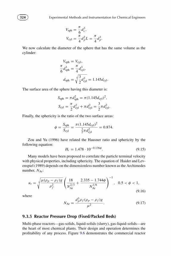
324 Experimental Methods and Instrumentation for Chemical Engineers
Vsph = π
6d3
s ,
Vcyl = π
4d2
p L = π
4d3
p.
We now calculate the diameter of the sphere that has the same volume as thecylinder:
Vsph = Vcyl,
π
6d3
sph = π
4d3
cyl,
dsph = 3
√3
2d3
cyl = 1.145dcyl.
The surface area of the sphere having this diameter is:
Ssph = πd2sph = π(1.145dcyl)
2,
Scyl = π
2d2
cyl + πd2cyl = 3
2πd2
cyl.
Finally, the sphericity is the ratio of the two surface areas:
φ = Ssph
Scyl= π(1.145dcyl)
2
32πd2
cyl
= 0.874.
Zou and Yu (1996) have related the Hausner ratio and sphericity by thefollowing equation:
Hr = 1.478 · 10−0.136φ. (9.15)
Many models have been proposed to correlate the particle terminal velocitywith physical properties, including sphericity. The equation of Haider and Lev-enspiel (1989) depends on the dimensionless number known as the Archimedesnumber, NAr:
ut = 3
√μ(ρp − ρ f )g
ρ2f
(18
N 2/3Ar
+ 2.335 − 1.744φ
N 1/6Ar
)−1
, 0.5 < φ < 1,
(9.16)where
NAr = d3pρ f (ρp − ρ f )g
μ2 . (9.17)
9.3.5 Reactor Pressure Drop (Fixed/Packed Beds)
Multi-phase reactors—gas-solids, liquid-solids (slurry), gas-liquid-solids—arethe heart of most chemical plants. Their design and operation determines theprofitability of any process. Figure 9.6 demonstrates the commercial reactor

325Chapter | 9 Analysis of Solids and Powders
FIGURE 9.6 Formaldehyde Multi-Tubular Fixed Bed Reactor (Image courtesy of Haldor-Topsøe)
to produce formaldehyde by the partial oxidation of methanol. The reactor isabout 2 m in diameter and it contains 10 000 tubes each with a diameter of22 mm. Catalyst pellets are charged to each tube. In the early 1960s and 1970s,spherical pellets of about 3 mm were used. Better productivity was achievedwith cylindrical pellets. The cylindrical pellets were modified by boring a holethrough the end to make an “elongated ring.” The motivation for changing thedimensions was twofold: (a) increase productivity and (b) decrease pressuredrop. The pressure drop, �P/�Z , across tubular reactors for spherical particlesis calculated based on Ergun’s equation:
�P
�Z= Ug
φdp
1 − εv
ε3v
(150(1 − εv)
μ
φdp+ 1.75ρgUg
), (9.18)
where Ug is the superficial gas velocity (velocity assuming the tube is absent ofparticles) in m s−1, εv is the void fraction, dp is the average particle diameterin m, μ is the fluid viscosity in Pa s, ρg is the gas density in kg m−3, and φ isthe sphericity.
By maximizing the particle diameter, the pressure drop is minimized.However, the rate of diffusion of heat and mass in and out of the particle ispoorer and therefore productivity suffers.
The Thiele modulus, φs , is a dimensionless number that relates the reactionrate to the diffusion rate. When the reaction is fast compared to diffusion,the Thiele modulus is high and the effectiveness factor, η, equals one—allof the catalyst is active. When the Thiele modulus is low, and the diffusionrate (mass transfer) is the controlling factor, the effectiveness factor of thecatalyst is below 1. The Thiele modulus is derived based on a mass balanceassuming the reaction is first order (proportional to the concentration of the

326 Experimental Methods and Instrumentation for Chemical Engineers
reacting species) and isothermal conditions. As shown, in the equation, φs isdirectly proportional to the particle diameter, decreases with the square rootof diffusivity, DE (m2 s−1), and increases with the first-order rate constant,k (s−1):
φs = dp
6
√k
DE= reaction rate
diffusion rate. (9.19)
The effectiveness factor is calculated according to Equation (9.20). For aThiele modulus of 2, the effectiveness factor is approximately 0.5 and it equals0.1 for a value of φs of 10:
η = 1
φs
(1
tanh (3φs)− 1
3φs
). (9.20)
Example 9.5. A plant produces formaldehyde from methanol in a multi-tubular reactor. The reactor contains 10 000 tubes. Each tube is 1.2 m longwith an inside diameter of 25 mm. The catalyst particles are spherical withan average diameter of 3 mm and the inter-particle void fraction equals 0.45.The reactor operates with 6.0 vol% MeOH in air at a temperature of 337 ◦C, apressure of 1.5 bara, and a superficial gas velocity of 2 m s−1:
(a) Calculate the pressure drop (assuming the volume change with reaction isnegligible).
(b) Calculate the effectiveness factor for a rate constant of 1.0 s−1 and adiffusivity of 0.007 cm2 s−1.
(c) What would the pressure drop and effectiveness factor be for a particle2 mm in diameter?
Solution 9.5a. The gas density, ρ f = M P/RT , equals 0.86 kg m−3. Since94% of the gas is air, we can assume that its viscosity is equal to that of air at thereactor operating temperature—0.000 033 Pa s. All other operating parameterswere defined in the problem. The pressure drop is calculated from Ergun’sequation:
�P = Ug
dp
1 − εv
ε3v
(150(1 − εv)μ
dp+ 1.75ρgUg
)�Z
= 2
0.003
1 − 0.45
0.453
(150(1 − 0.45) · 0.000033
0.003+ 1.75 · 0.86 · 2.0
)· 1.2
= 19 kPa.
Solution 9.5b. The Thiele modulus is:
φs = dp
6
√k
DE= 0.003 m
6
√1 s−1
0.007 cm2 s−1 · (0.01 m cm−1)2 = 0.60.

327Chapter | 9 Analysis of Solids and Powders
FIGURE 9.7 Pellet Morphology in Chemical Reactors (Image courtesy of Clariant.) (For colorversion of this figure, please refer the color plate section at the end of the book.)
The effectiveness factor equals:
η = 1
φs
(1
tanh (3φs)− 1
3φs
)= 1
0.60
(1
tanh (3 · 0.6)− 1
3 · 0.60
)= 0.83.
Solution 9.5c. For particles with a diameter of 2 mm, the pressure drop is32 kPa and the effectiveness factor becomes 0.92.
Whereas Figure 9.3 shows many different shapes that are common toengineering practice, Figure 9.7 shows the different particle shapes that areused in chemical reactors.
9.3.6 Fluidization
While the particle diameter of fixed bed reactors is on the order of 1–5 mm, theparticle size used in another type of reactor—fluidized bed reactors—is on theorder of 50–200 µm. Because of the small diameters, the effectiveness factoris close to 1 in most cases. The Ergun equation characterizes the pressure dropacross a bed of solids—at low gas velocities (relative to the particle terminalvelocity). When the drag force of the upward moving fluid exceeds the weightof the particles, the particles become fluidized—they begin to move up anddown and the solids bed itself behaves like a fluid: objects that are denser thanthe bed will fall through the bed while objects that are less dense will be remainat the top. Based on a force balance, the pressure drop across the bed, �P/L ,will be equal to the head of solids (neglecting frictional forces):
�P
Lm f= (ρm f − ρ f )g, (9.21)
where Um f is the minimum velocity at which the solids become fluidized, Lm f
is the height of the bed at minimum fluidization, and ρ f is the fluid density inkg m−3.

328 Experimental Methods and Instrumentation for Chemical Engineers
Considering that the mass of solids charged to the bed, W, is the product ofthe density and volume (V = Lm f X A):
W = ρm f V = ρm f Lm f X A. (9.22)
The pressure drop in the bed may be estimated based solely on the cross-sectional area and mass:
�P = gW
X A. (9.23)
For the case of very small particles, when the viscous forces dominate(NRe,m f < 20), the minimum fluidization velocity, um f , is given by:
um f = d2p(ρp − ρ f )g
150μ
ε2m f φ
2
1 − εm f, (9.24)
where
NRe,m f = ρ f um f dp
μ. (9.25)
When inertial forces dominate and viscous forces are negligible (NRe,m f >
1000):u2
m f = dp(ρp − ρ f )g
1.75ρ fε3
m f φ. (9.26)
When neither viscous nor inertial forces dominate, the equation relating theoperating conditions and particle properties is:
1.75
ε2m f φ
N 2Re,m f + 150(1 − εm f )
ε3m f φ
2NRe,m f = NAr. (9.27)
When εm f is unknown and for irregular shaped particles (unknown φ),Equation (9.27) may be written as (Kunii and Levenspiel, 1991):
K1 N 2Re,m f + K2 NRe,m f = NAr. (9.28)
For a large number of particles, Grace 1982 recommends that 1K1
= 0.0408
and K22K1
= 27.2. The minimum fluidization velocity is a parameter that isused in many correlations to predict mass transfer rates, heat transfer andother hydrodynamic characteristics. Particle diameter and shape are criticalparameters affecting um f .
Geldart (1973) studied the fluidization characteristics of many sorts ofpowders and then classified their behavior into four categories, as shown inFigure 9.8:
● Group A powders are considered aeratable, i.e. easily fluidizable. Typically,these particles have a diameter between 50 µm and 200 µm with a highfraction of fines (as much as 30%)—particles with a diameter between20 µm and 40 µm.

329Chapter | 9 Analysis of Solids and Powders
10 50 100 500 1000dp, mμ
10
5
1
0.5
0.1
p—g, g
/mL
ρρ
CCohesive
AAeratable
DSpoutable
BSand-like
FIGURE 9.8 Powder Classification of Geldart in Air at Ambient Conditions (Geldart, 1973)
● Group B powders have a higher density and/or particle size compared toGroup A powders. Sand is a typical example of a Group B powder.
● Group C powders are cohesive and fluidize with great difficulty. Theygenerally have a lower particle density and/or particle size compared toGroup A powders.
● Group D powders are difficult to fluidize—gas will channel through the bedand so shallow beds are common to minimize flow maldistribution.
9.4 PARTICLE SIZE DISTRIBUTION
The particle shape is only one factor in characterizing the average size of asample population. The second critical parameter is the particle size distribution.Examples of particle sizes that are reasonably uniform include basmati rice andgrain. For small particles however, the average population distribution mayrange from tens of µm to several hundred µm. This is particularly true forfluidized bed catalysts. (Fixed bed catalyst pellets—cylinders, for example—are generally considered to be monodispersed.) For polydispersed powders,selecting the appropriate diameter to represent the population is as difficult asselecting the appropriate shape for non-spherical particles.
9.4.1 Population of Particles
Algebraic expressions are used to reduce a population of particles with awide size distribution to a single value. The expression relies on a physicalcharacteristic of the population or a combination of characteristics—number,length (or some linear dimension representing the particle) area, mass, orvolume, assuming that the particle density is invariant with volume.

330 Experimental Methods and Instrumentation for Chemical Engineers�
�
�
�
TABLE 9.5 Distribution of Objects Orbiting the Earth(Wood-Kaczmar 1991)
Size (mm) Number of Objects % by Number % by Mass
100–10 000 7000 0.2 99.96
10–100 17 500 0.5 0.03
1–10 3 500 000 99.3 0.01
Total 3 524 500 100.0 100.00
For a given particle distribution, the distributions of sizes in number, mass,and surface may differ significantly. For example, consider objects in orbitaround the earth as summarized in Table 9.5. The majority of particles, some3 500 000, are from 1 mm to 10 mm in diameter—these particles represent99.3% of the total number of particles. However, they only account for 0.01%of the mass of particles orbiting earth. There are 7000 objects from 0.1 m to10 m and these objects account for 99.96% of the total mass. If we considermass, the average particle diameter is clearly between 0.10 m and 10 m, whileif we consider the total number of objects, the average size lies between 1 mmand 10 mm. The question is, which distribution is most appropriate to calculatethe characteristic diameter? The answer is that the diameter most representativeof the distribution depends on the application: how much (in terms of mass)versus how many. Clean rooms for electronic applications are concerned withhow many while catalytic reactors are concerned with how much.
Figure 9.9 illustrates the relationship between the size distribution functionF(dp) and the particle size, dp, in which the function represents the fractionof particles between dp and dp + �dp. The distribution of particles based onnumber is concentrated around the low particle sizes while the distributionbased on volume (or mass) has a distribution with a weighting toward the largerparticle size.
Several standard expressions of a population that are used include mode,median, and mean differences (arithmetic, geometric, square, harmonic, etc.),as shown in Figure 9.10.
The mode is the diameter that occurs most frequently and this value isthe smallest compared to all other representation of a population of particlesnormally distributed. It is infrequently used. The median is most often usedand represents the diameter for which 50% of the particles are smaller thanthat value (in terms of weight). It is also known as the d50. A d95 represents adiameter for which 95% of the particles are smaller than this value.
Besides the standard statistical representations of a population—mean,median, and mode—many other averaging techniques are used for powders.Consider a “population” of three particles with a diameter of 1 mm, 2 mm,

331Chapter | 9 Analysis of Solids and Powders
FIGURE 9.9 Distribution of Particles in Mass and Number
FIGURE 9.10 Different Options to Characterize the Size of Particles (According to Rhodes)
and 3 mm. The number length mean, dnl, is the arithmetic mean of the threeparticles:
dnl =∑
dp,i Ni∑Ni
= DN [1,0]. (9.29)
This value is also written as DN [1,0] and in the case of the three particles, itwill equal 2 mm. The first value in the expression DN [1,0]—one—refers to theexponent with respect to diameter in the numerator. The second value—zero—refers to the exponent with respect to diameter in the denominator.
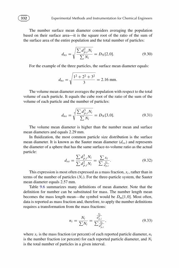
332 Experimental Methods and Instrumentation for Chemical Engineers
The number surface mean diameter considers averaging the populationbased on their surface area—it is the square root of the ratio of the sum ofthe surface area of the entire population and the total number of particles:
dns =√∑
d2p,i Ni∑Ni
= DN [2,0]. (9.30)
For the example of the three particles, the surface mean diameter equals:
dns =√
12 + 22 + 32
3= 2.16 mm.
The volume mean diameter averages the population with respect to the totalvolume of each particle. It equals the cube root of the ratio of the sum of thevolume of each particle and the number of particles:
dnv = 3
√∑d3
p,i Ni∑Ni
= DN [3,0]. (9.31)
The volume mean diameter is higher than the number mean and surfacemean diameters and equals 2.29 mm.
In fluidization, the most common particle size distribution is the surfacemean diameter. It is known as the Sauter mean diameter (dsv) and representsthe diameter of a sphere that has the same surface-to-volume ratio as the actualparticle:
dsv =∑
d3p,i Ni∑
d2p,i Ni
=∑
xi∑ xidp,i
. (9.32)
This expression is most often expressed as a mass fraction, xi , rather than interms of the number of particles (Ni ). For the three-particle system, the Sautermean diameter equals 2.57 mm.
Table 9.6 summarizes many definitions of mean diameter. Note that thedefinition for number can be substituted for mass. The number length meanbecomes the mass length mean—the symbol would be Dm[1,0]. Most often,data is reported as mass fraction and, therefore, to apply the number definitionsrequires a transformation from the mass fractions:
ni = Ni∑Ni
=xi
d3p,i∑ xid3
p,i
, (9.33)
where xi is the mass fraction (or percent) of each reported particle diameter, ni
is the number fraction (or percent) for each reported particle diameter, and Ni
is the total number of particles in a given interval.

333Chapter | 9 Analysis of Solids and Powders�
�
�
�
TABLE 9.6 Definitions of Number Mean Diameters (Allen 1990)
Designation Definition and Symbol
Number length mean diameter DN [1,0]: dnl =∑
dp,iNi∑Ni
Number surface mean diameter DN [2,0]: dns =√∑
d 2p,iNi∑Ni
Number volume mean DN [3,0]: dnv = 3
√∑d 3
p,iNi∑Ni
Length surface mean diameter DN [2,1]: dls =∑
d 2p,iNi∑
dp,iNi
Length volume mean diameter DN [3,1]: dlv =√∑
d 3p,iNi∑
dp,iNi
Surface-volume mean diameter DN [3,2]: dsv =∑
d 3p,iNi∑
d 2p,iNi
=∑
xi∑ xidp,i
(Sauter mean diameter—SMD)
Volume moment mean diameter DN [4,3]: dlv =√√√√∑
d 4p,iNi∑
d 3p,iNi
The mass numbers for our example with three particles are much closerthan the number distribution: the mass length mean diameter, Dm[1,0], equals2.72 mm. The mass surface mean diameter, Dm[2,0], is 2.77 mm and the massvolume mean diameter, Dm[3,0], is 2.80 mm.
Example 9.6. Table E9.6 summarizes the particle size distribution of commer-cial vanadium pyrophosphate catalyst to produce maleic anhydride from butanein a circulating fluidized bed reactor. Calculate DN [1,0],DN [2,0],DN [3,0],DN [3,2], and DN [4,3].
Solution 9.6. Figure E9.6S is a plot of the wt% of each fraction as a functionof the particle size and show a pseudo-bimodal distribution. There is a highfraction of fines and the highest fraction has a diameter of 55 µm. Because ofthe granularity of the particle size (small intervals between each particle size),a simple arithmetic mean of the upper and lower values is sufficient, i.e. theaverage particle diameter of the fraction between 32 µm and 44 µm is 38 µm.The Sauter mean diameter may be calculated directly from the data, since it isdefined by a number fraction as well as a mass fraction in Table 9.6. Note thatthe sum of the weight fraction is not 1 but 0.994! Table E9.6S lists the averageparticle diameter for each segment of the wt% as well as the percentage based

334 Experimental Methods and Instrumentation for Chemical Engineers�
�
�
�
TABLE E9.6 PSD for CommercialVanadium Pyrophosphate Catalyst
dp wt%
dp < 10 0
10 < dp < 20 1.3
20 < dp < 25 4.7
25 < dp < 32 11.5
32 < dp < 44 22
44 < dp < 66 32.8
66 < dp < 88 1.3
88 < dp < 100 4.6
100 < dp < 125 7.8
125 < dp < 150 5.5
150 < dp < 200 6.2
200 < dp < 250 1.7
on the number, N%. This value is calculated from the mass fraction as:
Ni∑Ni
=xi
d3p,i∑ xid3
p,i
.
D[1,0] = 30 µm,D[2,0] = 33 µm,D[3,0] = 37 µm,D[3,2] = 48 µm,
D[4,3] = 68 µm.
9.5 SAMPLING
The physical and chemical characteristics of several tons of material are oftenassumed based on a sample that may be no more than a couple of grams.The probability of withdrawing a representative sample is remote even whenstandardized procedures are followed with the same equipment and the sameoperator. Atmospheric monitoring is an example in which sampling is a criticalfactor that is mandated by government legislation. It is conducted to monitorhealth hazards and the EPA in the USA stipulates that the particulate mattershould be inferior to 75 µg m−3 on an average annual basis and that theinstantaneous maximum concentration should not exceed 260 µg m−3 (EPA,2011). Manufacturers must monitor and control their particulate discharge ratesincurring costs for cyclones, filters, scrubbers, electrostatic precipitators, etc.
Sampling can be broken into primary and secondary sampling. Primarysampling relates to removing a representative sample from the bulk—how toget a sample from a train car, drum, etc. ISO and other standards (ISO 13320 (3),
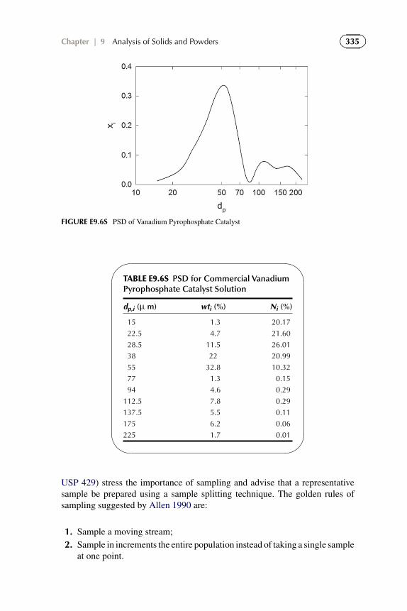
335Chapter | 9 Analysis of Solids and Powders
FIGURE E9.6S PSD of Vanadium Pyrophosphate Catalyst
�
�
�
�
TABLE E9.6S PSD for Commercial VanadiumPyrophosphate Catalyst Solution
dp,i (µ m) wti (%) Ni (%)
15 1.3 20.17
22.5 4.7 21.60
28.5 11.5 26.01
38 22 20.99
55 32.8 10.32
77 1.3 0.15
94 4.6 0.29
112.5 7.8 0.29
137.5 5.5 0.11
175 6.2 0.06
225 1.7 0.01
USP 429) stress the importance of sampling and advise that a representativesample be prepared using a sample splitting technique. The golden rules ofsampling suggested by Allen 1990 are:
1. Sample a moving stream;2. Sample in increments the entire population instead of taking a single sample
at one point.

336 Experimental Methods and Instrumentation for Chemical Engineers
Allen (1990) has defined the minimum mass of a sample to be collectedin terms of the particle size distribution, particle density, ρp (kg m−3) andmass fraction of the coarsest size class, wλ. For a size range less than
√2 : 1
(120 µm:85 µm, for example) and where the mass fraction of the coarsest sizeclass is less than 50 wt%:
ms = 1
2
ρp
σ 2
(1
wλ
− 2
)d3
p,λ · 106, (9.34)
where ms is the minimum sampling mass in kg, dp,λ is the arithmetic meanof the coarsest fraction in mm, and σ 2 is the variance of the sampling error(generally 5%).
Example 9.7. Approximately 40% of the oil produced in the world is crackedcatalytically to smaller molecules with zeolite catalysts—known as FCC (fluidcatalytic cracking). The catalyst has an average diameter around 70 µm andit becomes coarser with time as the fine fraction of the powder is lost in thecyclones. For a FCC unit containing 200 t of catalyst, what is the smallest samplesize required to achieve a sampling error less than 5% if the coarsest size rangeis from 177 µm to 210 µm. The particle density of FCC is 1200 kg m−3.
Solution 9.7. The arithmetic mean of the coarsest fraction is:
dp,λ = 1
2(177 + 210) = 194 µm.
Assuming the coarsest sample size represents 5% of the total mass, the samplesize to be collected, ms , is:
ms = 1
2
1200 kg m−3
0.05
(1
0.05− 2
)(0.194 mm3)3 · 10−6 = 0.016 kg.
The required sample size increases considerably as the coarsest fractiondecreases.
Secondary sampling is how we place a representative sample into theinstrument from the container that arrives in the laboratory. Care must be takenwith sampling when dispersing a powder into a liquid. Many methods callfor pre-dispersing the powder in a beaker and then pipetting the sample intothe analyzer. When following this approach it is better to mix a concentratedpaste in the beaker in order to minimize sampling bias during the transfer tothe analyzer. If this is not practical for whichever reason, then the beaker pre-dispersion should be continuously stirred and the sample should be extractedhalfway between the center of the beaker and the wall and also halfway betweenthe liquid surface and the bottom of the beaker.
Suspensions and emulsions can sometimes be easily measured using thecontinuous phase of the original sample as the diluent in the analyzer. Whenpowders are dispersed in liquid, the solvent must meet the following criteria:

337Chapter | 9 Analysis of Solids and Powders
● Negligible reactivity with powder;● Does not swell or shrink particles by more than 5% in diameter;● Solubility must be less than 5 g powder in 1 kg liquid;● Have a refractive index (RI) different than the sample;● Be free from bubbles and particles;● Have suitable viscosity to enable recirculation; and● Be chemically compatible with materials in the analyzer.
Dispersing powders in liquid can often present challenges. The ISO 14887standard provides useful insight into this realm. Among the suggestions in ISO14877 is to prepare the sample on a slide and look at it under a microscope.Determine if you are looking at individual particles or clumps. See if exposingthe sample to an external ultrasonic probe eliminates the clumps.
Surfactants are often required to wet the powder for proper dispersion. ISO14887 provides a comprehensive listing of commercially available dispersingagents. Some instrument manufacturers (Horiba, for example) recommendsurfactants including Micro 90 solution (also good for cleaning the instrument),Triton X-100, Igepal CA-630, Tween 80, and lecithin.
Once a powder is dispersed, it sometimes helps to add a stabilizer (oradmixture) to the sample, such as sodium hexametaphosphate. The stabilizeralters the charge on the surface of the particles, preventing re-agglomeration.
9.5.1 Stability Testing
After the dispersing liquid or mixture has been chosen, test the system forstability by collecting multiple measurements as a function of time. Measuringthe recirculating sample should generate extremely reproducible results. Thesample should be measured at least three times over a time frame of severalminutes. A particle size distribution which steadily shifts to a finer particle sidetogether with an increase in light transmission may indicate dissolution. Anincrease in particle size may indicate agglomeration or swelling. An increase intransmission alongside the disappearance of the coarsest particles may indicatesettling. Random variations are more difficult to interpret but could arise fromthermal fluctuations or poor mixing.
9.6 PSD ANALYTICAL TECHNIQUES
Techniques for analyzing the size and shape of particles and powders arenumerous. Some are based on the light, others on ultrasound, an electric field, orgravity. They can be classified according to the scope and scale of observation(Webb, 2011):
● Visual methods: Microscopy (optical, electronic, and electronic scanning)and image analysis;
● Separation methods: Screening, classification, impact and electrostaticdifferential mobility, sedimentation;

338 Experimental Methods and Instrumentation for Chemical Engineers
● Continuous scanning methods: Electrical resistance, optical detection zones;● Field scan techniques: Laser diffraction, sound attenuation, the photon
correlation spectroscopy;● Surface techniques: Permeability and adsorption.
It is important to define the characteristic dimension of each analyticaltechnique, some of which are reported in Table 9.7. Electro-zone techniqueswill typically report a volume average, Dm[3,0] and a number average DN [3,0].Most optical techniques report a surface dimension, DN [2,0], while microscopywill report a length dimension, DN [1,0] (although, if combined with imageanalysis, they also report a surface dimension). Sedimentation techniquesseparate particles based on the Stokes diameter. Sieve analysis separatespowders based on the narrowest projected surface area but sphericity canalso play a role for particles elongated in one direction. The mass of theparticles on each sieve is weighed, so the defining particle diameter would beDm[2,0]. When the distribution is not explicitly mentioned, it can be deducedby examining the population distribution curve. If the population of particlesat the low end is low, then most likely mass fractions are reported. When thefraction of the smallest particles is high, it is most likely that the particles arecounted.
Figure 9.11 shows the characteristic operating ranges of a selected numberof instruments. Sieve analysis is used for larger particles from as low as about10 µm to 1000 µm. Microscopy is adequate from below 1 µm to as muchas 1000 µm. For fine particles, laser diffraction is the most broadly acceptedtechnology and coincidentally can measure the widest range of particle sizes—itcan measure particles as small as low as 40 nm.
FIGURE 9.11 Range of Selected Measurement Techniques

339Chapter | 9 Analysis of Solids and Powders�
�
�
�
TABLE 9.7 Analytical Technique and Characteristic Dimension
Analytical Technique Size Range (µm) Representative Dimension
Sieving
Dry >10 Combination of Dm [2,0] and φ
Wet 2–500
Image analysis
Optical 0.2–100 DN [2,0]
Electron microscopy 0.01–500 DN [1,0] and DN [2,0]
Radiation scattering
Laser diffraction (Horiba) 0.01–3000 Dm [4.3], Dm [3,2]
Electrical zone sensing
(Coulter counter) 0.6–1200 DN [3,0], Dm [3,0]
1–800
Entrainment, elutriation
Laminar flow 3–75 Stokes diameter, dt
Cyclone 8–50
Gravity Sedimentation
Pipette 1–100
Photo-extinction 0.05–100 Stokes diameter
X-ray 0.1–130
Centrifugal classification 0.5–50 Stokes diameter
Agreement between analytical techniques is often poor. Moreover,reproducibility of measured distributions with the same technique but differentinstruments may be in disagreement by over 10%. Typically, when monitoringa process, or for quality control of the manufacture of a powder, the sameinstrument should be used and, whenever possible, the same operator. Betweentechnologies for non-spherical particles, on average laser diffraction (Horiba)will give a lower value compared to sieve analysis and an electrical zone sensing(Coulter counter):
(dsv)laser = 1.35(da)sieve = 1.2(dv)electrosensing. (9.35)
9.6.1 Sieve Analysis
Screening is one of the simplest, cheapest, and most commonly used techniquesto classify particles according to their size. It was one of the first separationtechniques used by ancient civilizations for the preparation of foodstuffs,

340 Experimental Methods and Instrumentation for Chemical Engineers�
�
�
�
TABLE 9.8 Standard US Mesh Sizes (McCabe and Smith, 1976)
Mesh µm Mesh µm Mesh µm
4 4760 20 840 100 149
5 4000 25 710 120 125
6 3360 30 590 140 105
7 2830 35 500 170 88
8 2380 40 420 200 74
10 2000 45 350 230 62
12 1680 50 297 270 53
14 1410 60 250 325 44
16 1190 70 210 400 37
18 1000 80 177 500 31
including the Egyptians. They were made of woven fabric and some were madeby punching holes in plates. Agricola illustrated woven wire sieves in 1556. In1867, Rittinger suggested a standardized progression of aperture size
√2 with
75 mm as the reference point. Between successive screens in a series, the openarea is double. Modern standards use a 4
√2 progression (1.189) (except for the
French AFNOR standard).Sieving separates powders solely based on their size—it is independent
of density or surface properties (although the sieving time may be a functionof density). Table 9.8 summarizes the sizes of the US Mesh from 31 µm to4760 µm.
To separate a powder into particle fractions, a series of sieves are stackedone on top of the other starting with a collection pan (receiver) followed by thescreen with the smallest aperture. The powder is weighed then poured on tothe top screen. A lid is placed on the top sieve and the stack is then shaken byhand (very inefficient) or vibrated with a machine. National standards BS1796,ASTM 452, and ASTM C136A each recommend different criteria for the lengthof time to vibrate. The first vibration period should be on the order of 20 min.After this point, the sieves are weighed and vibrated an additional 10 min. Ifthe change in weight from one period to another is greater than 0.5%, the stackshould be vibrated an additional 10 min (ASTM 452). Compressed air sieving isrecommended for particles up to 20 µm and wet sieving for particles that have atendency to form agglomerates. Wet sieving is useful for particles down to 5 µm.
The result of a sieve analysis is a tabulation of the mass of powder (or massfraction) of each screen increment. Two numbers are required to specify theparticle size: the screen through which the particles pass and the screen onwhich they are retained. The data may be reported as 120/170—the particleswere retained on the 170 mesh screen and passed through the 120 mess screen.
341Chapter | 9 Analysis of Solids and Powders
This would mean that the particles on the 170 mesh screen lie between 88 µmand 125 µm. This representation of the data is referred to as a “differentialanalysis.” In a cumulative analysis, the particles retained on each screen aresummed sequentially starting from either the receiver or the screen with thelargest aperture.
Since the particles must pass through an opening between wires forming asquare mesh, the most appropriate diameter to represent the size distributionwould be D[2,0].
Errors incurred during the sieving operation may include:
1. Insufficient duration;2. Wear on the sieves (thus allowing larger particles through a given sieve);3. Errors of sampling (the powder loaded to the stack is unrepresentative of
the populations);4. Measurement errors;5. Operational errors (too much or too little sample, humidity causing
agglomeration, or static);6. Sensitivity of powder to vibration (resulting in breakage); and7. Interpretation (particularly related to particle shape).
9.6.2 Laser Diffraction
Co-author: Mark BumillerLaser diffraction is the most popular, widespread modern sizing technology.
It has been used successfully for an array of applications across many industries.The current state-of-the-art instruments have a measurement range from 10 nmto 3 mm, the ability to measure suspensions, emulsions, and dry powders withinseconds, full push-button automation, and software. The instrument consists ofat least one source of high intensity, monochromatic light, a sample handlingsystem to control the interaction of particles and incident light, and an array ofphotodiodes to detect the scattered light over a wide range of angles.
The primary function of the array of photodiodes is to record the angle andintensity of scattered light. This information is then input into an algorithm thatconverts the scattered light data to a particle size distribution. The algorithmconsists of one of two optical models—the Fraunhofer approximation and theMie scattering theory—with the mathematical transformations necessary togenerate particle size data from scattered light. The Fraunhofer approximation,which enjoyed popularity in older laser diffraction instruments, assumes thatparticles:
● are spherical;● are opaque;● scatter equivalently at wide angles and narrow angles;● interact with light in a different manner than the medium.

342 Experimental Methods and Instrumentation for Chemical Engineers
These assumptions are reasonable for particles greater than 20 µm. TheMie scattering theory is a closed-form solution (not an approximation) toMaxwell’s electromagnetic equations for light scattering from spheres. Thissolution is superior to the Fraunhofer approximation: it has a much greatersensitivity to smaller particles (which scatter at wider angles); it includes awide range of particle opacity (i.e. light absorption); and, it is user-friendlysince only the refractive index of the particle and dispersing medium is required.Accounting for the light that refracts through the particle allows for accuratemeasurement even in cases of significant transparency. The Mie theory makescertain assumptions:
● all particles are spherical;● each particle is of the same material;● the refractive indices of particle and dispersing medium are known.
The over-reporting of small particles is a typical error seen when using theFraunhofer approximation.
9.6.3 Microscopy
Co-author: Milad AghabararnejadOptical microscopy is often used as an absolute method of analysis of particlesize, since it is the only method that allows on the one hand, to examine theparticles individually for shape and composition, and on the other hand, tomeasure the diameter with a resolution of 200 nm (for optical microscopes)and particle sizes as low as 5 µm. It can provide information on the sizedistribution in number and form. Different diameters can be measured: theequivalent diameter of Martin, dM , Feret diameter, dF , the diameter of theprojected area, da , etc. New microscopes use cameras to output a digital imagefor analysis. Below 5 µm, the images are blurred due to diffraction effects.
For particles less than 5 µm, other electron microscopy can be used, suchas transmission electron microscopy (TEM), which can measure particles up to1 nm, and scanning electron microscopy (SEM), which can measure particlesup to a few nanometers. In TEM, electrons penetrate the sample while for SEMan electron beam scans the surface resulting in secondary electron emission,backscattered electrons, light, and X-rays. SEM is faster than TEM and givesa greater three-dimensional depth. Magnifications reach as high as 100 000×with resolutions of 15 nm. Significant sample preparation is required for bothmicroscopy techniques.
9.6.4 Electrical Sensing Instruments
Electrical sensing instruments measure changes in electrical conductivity whenparticles pass through an orifice together with a conductive fluid. The magnitudeof the change in conductivity is representative of the particle size and the number

343Chapter | 9 Analysis of Solids and Powders
of particles passing the aperture equals the number of pulses detected. Theprinciple relies on suspending a powder in a liquid and circulating the suspensionthrough an orifice across which a voltage is applied. The capacitance changeseach time a particle passes the orifice.
The instrument is quite easy to use but there are certain limitations:
● The electrolyte must be compatible with the particle (no swelling, breaking,or dissolution);
● The method is slow relative to laser diffraction (but substantially faster thesieving);
● Dense or large particles may settle in the beaker and thus are not measured.
9.7 SURFACE AREA
Surface area, together with density and particle size, is a critical parameter inmany chemical engineering applications. It is a determining factor in makingcatalyst; moreover, the loss of surface area often correlates with loss in activity.
The theory of physical adsorption of gas molecules on solid surfaces wasderived by Brunauer, Emmett, and Teller (BET). The theory serves as the basisfor the most widely used technique to assess specific surface area of powdersand solids. It extends the Langmuir isotherm concept.
The BET theory accounts for monolayer and multilayer molecularadsorption according to the following hypotheses: (a) gas molecules physicallyadsorb on a solid in layers infinitely; (b) there is no interaction between eachadsorption layer; and (c) the Langmuir theory can be applied to each layer. Theresulting BET equation is expressed by:
1
W(
P0P − 1
) = c − 1
Wmc
P
P0+ 1
Wmc, (9.36)
where P and P0 are the equilibrium and the saturation pressure of adsorbatesat the temperature of adsorption, W is the adsorbed gas quantity, and Wm is themonolayer adsorbed gas quantity. c is the BET constant, which is expressed by:
c = exp
(E1 − EL
RT
), (9.37)
where E1 is the heat of adsorption for the first layer, and EL is that for the secondand higher layers and is equal to the heat of liquefaction. Equation (9.36) is anadsorption isotherm and can be plotted as a straight line with 1
W(
P0P −1
) on the
y-axis and φ = PP0
on the x-axis.
The linear relationship of this equation is maintained only in the range of0.05 < P
P0< 0.35. The value of the slope A and the y-intercept I of the line

344 Experimental Methods and Instrumentation for Chemical Engineers
are used to calculate the monolayer adsorbed gas quantity Wm and the BETconstant c. Consider I and A as intercept and slope of the BET plot:
Wm = 1
A + I, (9.38)
c = 1 + A
I. (9.39)
The BET method is widely used in surface science for the calculation ofsurface areas of solids by physical adsorption of gas molecules. The total surfacearea, Stotal, is evaluated by the following equation:
Stotal = Wm N A
M, (9.40)
where N is Avogadro’s number (6.022 × 10²³ molecule mol−1), A is the areaof the cross-section of adsorbate molecules (16.2 A2 mol−1 for nitrogen), andM is the molecular weight of the adsorbent gas in g mol−1.
The measured surface area includes the entire surface accessible to the gaswhether external or internal. Prior to the measurement, the sample is pre-treatedat high temperature in vacuum in order to remove any contaminants. To causesufficient gas to be adsorbed for surface area measurement, the solid must becooled (normally to the boiling point of the gas). Most often, nitrogen is theadsorbate and the solid is cooled with liquid nitrogen. Adsorption continuesuntil the amount of nitrogen adsorbed is in equilibrium with the concentrationin the gas phase. This amount is close to that needed to cover the surface in amonolayer (see Table E9.2).
Example 9.8. An α-alumina powder with an average dp of 130 µm and totalsurface area of 46 m2 g−1 is impregnated by an 8 M solution of nickel nitrate
FIGURE E9.8S Seven Adsorption Point BET Plot

345Chapter | 9 Analysis of Solids and Powders�
�
�
�
TABLE E9.8 BET Results (P in mmHg, Volume in cm3)
Run 1 (m = 0.2413 g) Run 2 (m = 0.2251 g) Run 3 (m = 0.2482 g)P Adsorbed P Adsorbed P Adsorbed
(P0 = 768) Volume N2 (P0 = 780) Volume N2 (P0 = 769) Volume N2
45 1.6 41 1.3 45 1.6
63 1.7 64 1.4 63 1.7
83 1.8 85 1.5 83 1.8
118 2.0 123 1.6 119 2.0
157 2.2 162 1.7 157 2.1
196 2.3 200 1.8 197 2.3
235 2.4 239 1.9 234 2.5
hexahydrate Ni(NO3)2 · 6H2O. A seven-point BET test was completed usingnitrogen as adsorbate on the impregnated powders. The BET test was repeatedthree times and Table E9.8 represents the volume of adsorbed nitrogen atdifferent pressures. Calculate the total surface area.
Solution 9.8. The first step is to plot 1
W( P0
P −1) versus P
P0. W is the mass of
adsorbed nitrogen per mass of sample (in g). Table E9.8S shows the calculatedvalue for the first run.
�
�
�
�
TABLE E9.8S First RunPP0
W 1W(
P1P −1
)
0.058 0.0081 7.7
0.082 0.0087 10.3
0.108 0.0093 12.9
0.154 0.0102 17.8
0.205 0.0111 23.2
0.256 0.0119 28.8
0.306 0.0127 34.8
Nitrogen is considered an ideal gas. Figure E9.8S shows the BET plot ofthe first run.
346 Experimental Methods and Instrumentation for Chemical Engineers
Using a linear regression, the slope is:
A = 108.7
the intercept is:I = 1.2
and the correlation coefficient is:
r = 0.999,
Wm = 1
A + I= 1
108.7 + 1.2= 0.009
g N2
g sample,
Stotal = Wm N A
M=(
0.009 g N2g sample
)· 6.022 × 1023 · 16.2 × 10−20 m2
mol N2
28.0134 g N2mol N2
= 31.7m2
g sample.
The same procedure can be used for the second and third runs. The surfaceareas of the three runs are (in m2 g−1): 31.7, 26.7, and 31.4.
9.8 EXERCISES
9.1 Calculate the total void fraction of bulk solids if both the inter- and intra-void fractions equal 0.4.
9.2 To evaluate the particle density using a 100 ml graduated cylinder, it isfirst “calibrated” with water: the meniscus reached 98.3 ml when exactly100.0 g of water is charged to it at 20 ◦C. The procedure to measurethe particle density involves first drying the cylinder, adding 50 g ofwater, then measuring approximately 25 g of powder and pouring it intothe cylinder, and then finally adding water until it reaches the 98.3 mlmark. Calculate the particle density and uncertainty for the followingfive measurements:
● Initial mass of water: 50.3, 50.9, 48.7, 50.2, and 49.5.● Mass of catalyst added: 23.9, 25.2, 27.3, 24.8, and 26.3.● Mass of water added to 98.3 ml: 37.0, 37.8, 36.9, 38.0, and 37.5.
9.3 Determine the Hausner ratio and its uncertainty for a 100.0 g sample ofcatalyst that is poured into a 100 ml graduated cylinder. Based on the Zouand Yu correlation, what is the sphericity of the catalyst particles:
● Poured height: 87.3, 86.9, 88.5, 87.0, and 85.8.● Tapped height: 80.2, 80.9, 81.3, 80.3, and 79.8.
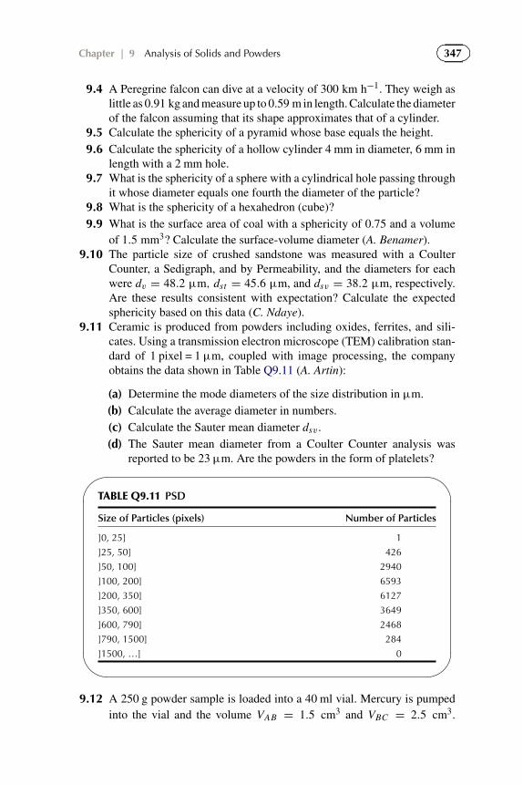
347Chapter | 9 Analysis of Solids and Powders
9.4 A Peregrine falcon can dive at a velocity of 300 km h−1. They weigh aslittle as 0.91 kg and measure up to 0.59 m in length. Calculate the diameterof the falcon assuming that its shape approximates that of a cylinder.
9.5 Calculate the sphericity of a pyramid whose base equals the height.9.6 Calculate the sphericity of a hollow cylinder 4 mm in diameter, 6 mm in
length with a 2 mm hole.9.7 What is the sphericity of a sphere with a cylindrical hole passing through
it whose diameter equals one fourth the diameter of the particle?9.8 What is the sphericity of a hexahedron (cube)?9.9 What is the surface area of coal with a sphericity of 0.75 and a volume
of 1.5 mm3? Calculate the surface-volume diameter (A. Benamer).9.10 The particle size of crushed sandstone was measured with a Coulter
Counter, a Sedigraph, and by Permeability, and the diameters for eachwere dv = 48.2 µm, dst = 45.6 µm, and dsv = 38.2 µm, respectively.Are these results consistent with expectation? Calculate the expectedsphericity based on this data (C. Ndaye).
9.11 Ceramic is produced from powders including oxides, ferrites, and sili-cates. Using a transmission electron microscope (TEM) calibration stan-dard of 1 pixel = 1 µm, coupled with image processing, the companyobtains the data shown in Table Q9.11 (A. Artin):
(a) Determine the mode diameters of the size distribution in µm.(b) Calculate the average diameter in numbers.(c) Calculate the Sauter mean diameter dsv .(d) The Sauter mean diameter from a Coulter Counter analysis was
reported to be 23 µm. Are the powders in the form of platelets?�
�
�
�
TABLE Q9.11 PSD
Size of Particles (pixels) Number of Particles
]0, 25] 1
]25, 50] 426
]50, 100] 2940
]100, 200] 6593
]200, 350] 6127
]350, 600] 3649
]600, 790] 2468
]790, 1500] 284
]1500, …] 0
9.12 A 250 g powder sample is loaded into a 40 ml vial. Mercury is pumpedinto the vial and the volume VAB = 1.5 cm3 and VBC = 2.5 cm3.

348 Experimental Methods and Instrumentation for Chemical Engineers
Calculate the skeletal density, the particle density, and the bulk density(R. Tohmé).
9.13 The results of a particle size analysis are shown in Table Q9.13:�
�
�
�
TABLE Q9.13 Salt Particle Size Analysis
Mesh dp (µm) Weight of Retained Particles (g)
20 840 0
30 590 4.8
40 420 8.9
60 250 24
80 177 19
120 125 12
140 105 5.7
(a) What is the d50 for this powder.(b) Calculate the DN [1,0] and DN [3,2] for the powder that passes through
the 40 Mesh sieve.
9.14 By controlling the precipitation conditions, zinc oxide particles will forman octahedral shape with a narrow particle size distribution (R. Silverwood):
(a) Calculate the sphericity of an octahedral particle.(b) Based on Table Q9.14, calculate the D[3,2].�
�
�
�
TABLE Q9.14 PSD of Zinc Oxide
dp (µm) Fraction
5 < dp � 10 0.09
10 < dp � 15 0.37
15 < dp � 20 0.42
20 < dp � 25 0.12
(c) What is the average particle diameter?
9.15 The measured diameters (dp) of a group of powders are: 0.12, 0.13, 0.14,0.14, 0.15, 0.13, 0.12, 0.12, 0.11, 0.14, 0.15, 0.15, 0.13, 0.11, 0.20, and0.13. Calculate dnl, dn−sa, dn−v , and dsv . Based on Chauvenet’s criterion,can you reject one of the measurements?

349Chapter | 9 Analysis of Solids and Powders
9.16 Derive the expression for the minimum fluidization velocity for the casewhere viscous forces dominate.
9.17 What is the particle terminal velocity in air of sand that is 150 µm indiameter? 60 µm in diameter? 30 µm in diameter?
9.18 Calculate the Archimedes number and the terminal velocity of a grain ofsand 250 µm in diameter in water.
9.19 A new process to convert glycerol to acrolein uses a catalytic fluidizedbed reactor:
C3H8O3 → C3H4O + 2H2O.
The particle size distribution is given in Table Q9.19:
(a) Calculate the hydraulic diameter and the Sauter mean diameter.(b) Of the four particle types given below, which has the greatest surface
area?(c) Which particle has the smallest surface area?(d) Is the charge loss in a tubular reactor greater for particle (i) or (ii)?(e) Is the charge loss in a tubular reactor greater for particle (ii) or (iii)?(f) What is the equivalent diameter and the sphericity of particle (iv)?
Particles:
(i) Sphere of diameter dp.(ii) Cylinder of diameter and height dp.(iii) Hollow cylinder of inner diameter dp/2, full diameter dp, and
height dp.(iv) Sphere of diameter dp with a hole of diameter dp/4 passing
through it.
�
�
�
�
TABLE Q9.19 Catalyst Particle Size Distribution
45 < dp � 68 4.7
68 < dp � 89 16.6
89 < dp � 102 15.5
102 < dp � 117 16.7
117 < dp � 133 15.3
133 < dp � 153 11.9
153 < dp � 175 8.1
175 < dp � 200 5.0

350 Experimental Methods and Instrumentation for Chemical Engineers
9.20 Demonstrate the equivalence of the two expressions of the Sauter meandiameter:
DN [3,2] = dsv =∑
d3p,i d N∑
d2p,i d N
and
dsv = 1∑ xidp,i
.
9.21 Methanol is produced in a tubular reactor with a Cu-Zr-Zn catalyst. Theparticle size distribution is obtained from sieving (see Table Q9.21).
d P
d Z= − Ug
φdp
1 − εv
εv
(150(1 − εv)
φdpμ + 1.75ρ0Ug
),
where εv = 0.41 ± 3%, μ = 0.000030 Pa s ± 3%, Z = 3.2 m, Ug =(2.0 ± 0.2) m s−1, ρ0 = 1.0 kg m−3, and φ = 0.95 ± 0.05:
(a) What definition of average particle is the most appropriate to char-acterize these particles? What characteristic diameter represents theflow rate of a tubular reactor?
(b) What is the average diameter and the charge loss across the bed?(c) The charge loss across the bed is greater than predicted according to
the calculations in (b). Identify three possible reasons for this.(d) Calculate the uncertainty in the charge loss taking into account the
uncertainties.
�
�
�
�
TABLE Q9.21 Particle Size Analysis by Sieving
Mesh dp (µm) Mass % Uncertainty (%)
4 4760
6 3360 10 1
10 2000 20 2
12 1680 30 3
14 1410 20 2
18 1000 20 2

351Chapter | 9 Analysis of Solids and Powders
REFERENCES
Allen, T., 1990. Particle Size Measurement, fourth ed. Chapman and Hall.ASTM 452, 2008. Standard Test Method for Sieve Analysis of Surfing for Asphalt. Roofing
Products.ASTM C136A, 1994. Field Sampling and Laboratory Testing Procedures Rejuvaseal Pavement
Sealer.BS1796, 1989. Test sieving. Methods using test sieves of woven wire cloth perforated metal plate.Geldart, D., 1973. Types of gas fluidization. Powder Technology 7 (5), 285–292. doi:
http://dx.doi.org/10.1016/0032-5910(73)80037-3.Grace, J.R., 1982. In: Hetsroni, G. (Ed.), Handbook of Multiphase Systems, Hemisphere, p. 8-1.Haider, A., Levenspiel, O., 1989. Drag coefficient and terminal velocity of spherical and non-
spherical particles. Powder Technology 58, 63–70.ISO 13320, 1999. Analyse granulométrique—Méthode par diffraction laser—Partie 1: Principes
généraux.ISO 14887, 2000. Sample preparation—dispersing procedures for powders in liquids.ISO 9276-6, 2008. Representation of results of particle size analysis—Part 6: Descriptive and
quantitative representation of particle shape and morphology.Kunii, D., Levenspiel, O., 1991. Fluidization Engineering. Butterworth-Heinemann Series in
Chemical Engineering, second ed.McCabe, W.L., Smith, J.C., 1976. Unit Operations of Chemical Engineering. McGraw-Hill
Chemical Engineering Series, third ed.EPA, 2011. Particulate Matter Sampling. Retrieved 2011 from APTI435:ATMOSPHERIC
SAMPLING COURSE:<http://www.epa.gov/apti/Materials/APT%20435%20student/Student%20Manual/Chapter_4_noTOC-cover_MRpf>.
Patience, G.S., Hamdine, M., Senécal, K., Detuncq, B., 2011. Méthodes expérimentales etinstrumentation en génie chimique, third ed. Presses Internationales Polytechnique.
van Oss, H.G., 2011. United States Geological Survey, Mineral Program Cement Report, January.USP 429. Light Diffraction Measurement of Particle Size.Webb, P.A., 2011. Interpretation of Particle Size Reported by Different Analytical Techniques,
Micromeritics Instrument Corp. Retrieved 2011 from Particle Size: <http://www.micromeritics.com/pdf/mas/interpretation%20of%20particle%20size%20by%20different%20techniques.pdf>.
Wood densities, n.d.. Retrieved 2011, from The Engineering ToolBox:<http://www.engineeringtoolbox.com/wood-density-d_40.html>.
Wood-Kaczmar, B., 1991 The junkyard in the sky: space is full of rubbish. From tiny flecks of paintto the broken remains of old satellites and rockets, the debris orbiting the Earth could mean theend of spaceflight within decades. New Scientist, October 13.
Yang, W.-C., 2003. Particle dharacterization and dynamics, Handbook of Fluidization and Fluid-Particle Systems. Marcel Dekker.
Zou, R.P., Yu, A.B., 1996. Evaluation of the packing characteristics of monosized nonsphericalparticles. Powder Technology 88, 71–79.

Solutions
CHAPTER 1
1.1 (a) 10.73 ft3 psi lb-mol−1 ◦R−1 (b) 0.082056 atm l mol−1 K−1
1.3 2.86 atm1.5 0.8 kPa1.7 (a) 74 µm (b) 246 µm1.9 (a) Your mass on the Moon is the same as on Earth—72.6 kg. The scale
would read a “weight” of one-sixth that: 12.1 kg. Force is the equivalentof weight in SI with the unit of N. Therefore, your “weight” on the Moonwould be 119 N (b) 72.6 kg
CHAPTER 2
2.1 (a) 3.2 × 10² (b) 15.3 (c) 1530 (d) 1.262.3 μ = 28.5, σ = 9.9, α = −1.87, P(Z < −1.88) = 0.470, we can
reject 102.5 0.0812.7 0.04 mV2.9 (a) μ = 112.7273, σ 2 = 1247.11, σ = 35.31 (b) no
2.11 PO2= 0.150 atm, WO2
= 0.001 atm2.13 t = 23.43 min, Wt = 1.732.15 (a) VC = 50.9 ml (b) �E = 0.0472 (c) �I = 0.0103 (d) Reading errors
and not respecting significant figures.2.17 (a) μ = 156.6, σ = 31.75, σ 2 = 1008.09 (b) 0.1664 (c) We can reject
902.19 η = 25.2127 mPa s,Wη = 1.0186 mPa s
353

354 Solutions
2.21 56 min 30 s2.23 (a) μ = 20.28, σ 2 = 10.17, σ = 3.19 (b) Yes, we can reject 12 because:
P
(xm − μ
σ
)= P
(12 − 20.28
3.19
)= P( − 2.6) = 2(0.495) = 0.99
and
1 − 0.99 <1
2(10)
(c)
μ =(7850 − 850) 1
3 · 4π(
1.5100
)3 · 9.81 · 20.28
6π 1.5100 · 0.4
= 174.08
Wρ−ρo =√
W 2ρ + W 2
ρo= 4 kg
Wμ
μ=
√(Wρ−ρo
ρ − ρo
)2
+(
Wt
t
)2
=√(
4
7000
)2
+(
2 · 3.19
20.28
)2
= 0.31
Wμ = 0.31
CHAPTER 3
3.1 (a) Five (b) Although the model has different values for the exponents,these are not strictly fitted parameters since they are not allowed to vary.The equation is a nonlinear model with four fitted parameters.
3.3 (a)
H0 : μ1 > μ2 + δ
H1 : μ1 � μ2 + δ
(b) If we take a value of δ = 0.2:
μ1 − μ2 = 0.2μ1 = 1.4
X1 − X2 − t(α,d f )
√S2
1
n+ S2
2
n< μ1 − μ2 < X1 − X2
+ t(α,d f )
√S2
1
n+ S2
2
n
6.90 − 6.44 − 2.26
√0.03 + 0.06
10< δμ1 < 6.90 − 6.44

355Solutions
+ 2.26
√0.03 + 0.06
100.23 < 1.4 < 0.89
Thus we can accept the null hypothesis. If we had defined δ = 0.1, thenwe would have rejected the null hypothesis and accepted the alternativethat Basmati is longer than UB. (c) Discuss.
3.5 (a) See Table QS9.5a (b) See Table QS9.5b (c) There is a confoundingfactor for (a) with the second and third models. The columnscorresponding to β0 and β11 X2
1 are parallel. There is also a confoundingfactor for (b) with the first and third models. The columns correspondingto β3 X3 and β12 X1 X2 are parallel (d) Part (a) with the third model andthe base case presents no confounding. Part (b) with the third model andthe base case does present confounding.�
�
�
�
TABLE QS9.5a Eight Experiments UsingTwo-Level Full Factorial Design
−1 −1 −1
−1 −1 1
−1 1 −1
−1 1 1
1 −1 −1
1 −1 1
1 1 −1
1 1 1
�
�
�
�
TABLE QS9.5b Eight Experiments UsingThree-Level Full Factorial Design
−1 −1 1
−1 0 0
−1 1 −1
0 −1 0
0 1 0
1 −1 −1
1 0 0
1 1 1
3.7 (a) There will be four parameters and the model will be of the followingform:
E = a1ε + a2T + a3 F + b

356 Solutions
(b) A minimum of four experiments are required to obtain the fourparameters. Eight experiments are needed for a full factorial design. Itis outlined in Table QS9.7. (c) The new model will have six parametersand be of the following form:
E = a1ε + a2T + a3 F + a12εT + a13εF + b
(d) A minimum of six experiments must be performed to obtain the sixparameters. 25 experiments are required for a full factorial design, whichis 32. �
�
�
�
TABLE QS9.7 Full Factorial Design for theFour Parameters
Exp E T F
1 1 1 1
2 1 1 −1
3 1 −1 1
4 1 −1 −1
5 −1 1 1
6 −1 1 −1
7 −1 −1 1
8 −1 −1 −1
3.9
P = 140 + 0.905Lt − 45.1Ct − 0.187Lt Ct
R2 = 0.9889
3.11 (a) The resistance depends on the concentration. (b) 20% (c) No3.13 (a) See Table QS9.13. (b)
� =
⎛⎜⎜⎜⎝
1 1 1 1
1 1 −1 −1
1 −1 1 −1
1 −1 −1 1
⎞⎟⎟⎟⎠
(c)Y = �θ⎛
⎜⎜⎜⎝Y (1)
Y (2)
Y (3)
Y (4)
⎞⎟⎟⎟⎠ =
⎛⎜⎜⎜⎝
1 1 1 1
1 1 −1 −1
1 −1 1 −1
1 −1 −1 1
⎞⎟⎟⎟⎠
⎛⎜⎜⎜⎝
β0
β1
β2
β12
⎞⎟⎟⎟⎠

357Solutions �
�
�
�
TABLE QS9.13 Factorial Design for theRelationship between Temperature,Pressure, and Quantity of Solvent toProduce Pesticide
Exp X1 X2
1 1 1
2 1 −1
3 −1 1
4 −1 −1
3.15 (a) Null hypothesis: Ho : μ1 = μ2 = μ3 = μ4, and the alternativehypothesis is that the means differ (b) Yes (c) Yes
3.17 (a) α = 2.8 (b) R2 = 0.9933.19
Em f = 1.53 + 0.0436T
R2 = 0.972
Em f = 0.045T
R2 = 0.94
Em f = 0.0365T + 0.0000416
R2 = 0.9993
CHAPTER 4
4.1
P = 1
3nMv2
rms = 1
3
n
VMv2
rms
Mv2rms = 3k N T
P = 1
3
n
V· 3k N T
PV = nk N T = n RT
R = k N
4.3 P = 0.32 atm,PO2= 0.067 atm
4.5 126.6 kPa4.7 (a) 771 mbar (b) 20.2 m (c) 0.16 m (d) 5.6 mm4.9 �P = 1.1 MPa,�P = 1800 Pa
4.11 (a) PA = 0.637 atm, PB = 2.81 atm, PC = 0.877 atm, PD = 16.0 atm(b) W�P = 1.08 atm

358 Solutions
4.13 18.74 kPa4.15 (a) 2 atm (b) The Nonette (c) 85 m (d) Same height4.17 t = 0.41 mm4.19 (a) H = 1.96 kPa, H = 6.13 kPa, H = 10.3 kPa (b) Glycerol4.21 0.0326 m4.23 (a) 0.007 mm, (b) 20. kPa, (c) 2.0 m, (d) 0.030 mm, (e) 0.06 − 6%@ FS
CHAPTER 5
5.1 (a) T = 45.4 ◦C (b) P2 = 173.79 kPa5.3 (a) Toluene (b) Galinstan (c) Toluene, 10X5.5 (a) No (b) 2.822 mV5.7 (a) r = 2
3t
(α2−α1)(T −T0)(b) 2.43
5.9 (�R
R
)2
=(
1
R0�R0
)2
+(
a + 2bT
1 + aT + bT 2 �T
)2
5.11 −0.1275 + 0.0415T + 1.226 × 10⁻⁷T 2,R2 = 0.999945.13 J: 0.663 mV, T: 0.513 mV, K: 0.519 mV, and J: 8 ◦C, T: 8.25 ◦C, K: 8.5 ◦C5.15 (a) 12.183 mV (b) 205.7 ◦F (96.5 ◦C) (c) 13.145 mV5.17 (a) T: T = 24.01�E + 25.03, K: T = 24.41�E + 24.99 (b) See
Table QS5.17 (c) Assuming the experiment was well conducted, thethermocouples should have a greater error (wT ) than calculated in (b).
�
�
�
�
TABLE QS5.17 Absolute and Relative Errors for Each Device (T and wTin ◦C, relative error in %)
Exp. Therm. Type T Type KT wT Rel. Err. T wT Rel. Err. T wT Rel. Err.
21 0.5 2 21.4 0.1 0.6 21.4 0.1 0.6
25 0.5 2 26.0 0.1 0.5 25.7 0.1 0.5
29 0.5 2 29.2 0.1 0.4 29.7 0.1 0.4
33 0.5 2 33.4 0.1 0.4 35.0 0.1 0.3
39 0.5 1 38.3 0.1 0.3 38.5 0.1 0.3
42 0.5 1 42.4 0.1 0.3 42.5 0.2 0.6
47 0.5 1 46.9 0.1 0.2 46.5 0.1 0.3
51 0.5 1 50.4 0.1 0.2 49.9 0.1 0.2

359Solutions
CHAPTER 66.1 (a) ��P = 21 Pa (b) Q = 5.40 × 10⁻³ m3 s−1 (c) �Q = 1.3%6.3 Pipe 1: 105.9 l min−1 at STP, pipe 2: 139.3 l min−1 at STP. The flow rate
is higher for the second pipe.6.5 (a) 657 Pa (b) Turbulent (c) 1%6.7 Q = 596202.31 ml s−1, m = 24.03 g s−1
6.9 u = 6 m s−1,m = 84 kg s−1
6.11 0.051 m3 s−1
6.13 (a) 27.4% of the height (b) Steel: 43% of the height, tantalum: 30% of theheight
6.15 0.55% ∼ 6%6.17 Pdyn = 0.45 mbar,�u1 = 0.0166 m s−1
6.19 14 m s−1
CHAPTER 7
7.1 (a) 0.010 m s−1 (b) �u = 0.0006 m s−1 (c) 17 800 kg m−3
(d) 17.1 karats (e) Yes (f) Take more data points, prolong the time thefalling ball falls, use a more viscous oil.
7.3 (a)
q
A= k
�T
�x
�x = k�T
q/A
W�x
�x=
√(Wk
k
)2
+(
W�T
�T
)2
+(
Wq/A
q/A
)2
W�x =√
0.052 +(
0.2
15
)2
+ 0.012 · 10 cm = 0.53 cm
(b) �T2 = 2 qA
�xk = 2�T1 = 30 ◦C (c) The uncertainty of the
temperature measurement is incorrect, or the heat flux is 2.2 or 10%instead of 1%.
7.5 k2 =− Tm−T1Tm−T2
k1, so k2 = 3.5 W m−1 K−1 and Wk2 = 0.085 W m−1 K−1
7.7 (a) If the walls of the process in which the refrigerant circulates are notisolated, it is impossible to determine the thermal coefficient because thereis heat loss to the environment (b) k = 1.03 k W m−1 ◦C−1
7.9 (a) ρ = 8784 kg m−3
7.11 (a) Air (b) T, F, F (c) T, T, T (d) 1C, 2B, 3A, 4D (e) F, T, F, F (f) gases,liquids, plastics, alloys, metals (g) F, T, F

360 Solutions
7.13 (a) 13.3, 0.54 (b) μ= (ρ−ρ0)V g6πr L t = (4540−970)·2·0.012·9.81
9·0.4 ·13.3 = 25.9 Pa s
(c) �= k(α)σ =2.57 · 0.54 = 1.4 s (d) Wμ/μ = √(Wρ/ρ)2 + (Wt/t)2
= √(20/3570)2 + (1.4/13.4)2 = 0.10 = 10%,Wμ = 0.1 · 25.9
= 2.6 Pa s (e)
a = X − μ
σ= 14.1 − 13.3
0.54= 1.48
P(Z < 1.48) = 0.431
5(1−2 ·0.431) = 0.691 > 0.5, therefore accept. t is 13.4 s, 12.9 s, 14.1 s,12.7 s, and 13.2 s.
CHAPTER 8
8.1 (a) 836 plates (b) 0.066 mm (c) 1.57 (d) 1502 plates (e) 84.61 cm8.3 (a) 2858 ml, 221.3 ml min−1, 52.5 min, 0.982 (b) 18.23 ppm. The con-
centration is too high. The desulfurization unit must be revised to have abetter process efficiency.
8.5 (a) C = 0.0016 mol l−1 (b) C ′ = 0.0008 mol l−1
8.7 (a) t0 = 0.8 min, t1 = 3.2 min, t2 = 6 min, t3 = 18 min, k1 = 3, k2 =6.5, k3 = 21.5 (b) Nth = 5.54(tr/w1/2)
2, so Nth,1 = 5700,Nth,2 =3200,Nth,3 = 55 400 (c) R = 9.4, the minimum value is 1.25 although1.5 is accepted, shorten the column, increase the temperature, increase thelinear velocity of the mobile phase, and decrease the amount of stationaryphase (d) �S
S = 5%8.9 (a) Reduce the analysis time. (b) Solute diffusion is faster than in N2, so the
balance between the mobile phase and the stationary phase is reached morequickly. For DCT it is easier to detect higher resolution. Conductivity.(c) Detectable: alcane, organic; undetectable: oxygen, nitrogen, carbondioxide, etc. (d) 8 or 9, k′ is 13.5, 18, and 21, α1,2 = 1.33, α1,3 =1.56, α2,3 = 1.17, R2,1 = 1.89 > 1.25 so it is well resolved,R3,2 = 1.13 < 1.25 so it is not well resolved
8.11 (a) Nth = 2544,N 2
th4 = 12.61, L = 13 cm (b) k′ = 1.5, k′
k′+1 = 0.6(c) R = 7.41 > 1.5, there is separation.
8.13 See Fig. QS8.13
CHAPTER 9
9.1 0.689.3 H = 1.08, �H = 0.02, φ = 1
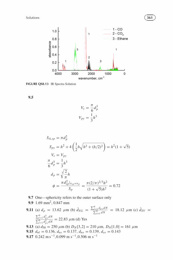
361Solutions
FIGURE QS8.13 IR Spectra Solution
9.5
Vs = π
6d3
p
Vpy = 1
3h3
SA,sp = πd2p
Spy = h2 + 4
(1
2h√
h2 + (h/2)2
)= h2(1 + √
5)
Vs = Vpy
π
6d3
p = 1
3h3
dp = 3
√2
πh
φ = πd2sp|vsp=vp
Sp= π(2/π)2/3h2
(1 + √5)h2
= 0.72
9.7 One—sphericity refers to the outer surface only9.9 1.69 mm2, 0.847 mm
9.11 (a) dp = 13.62 μm (b) dN L =∑9
i=1 dp,i d N∑9i=1 d N
= 18.12 μm (c) dSV =∑9i=1 d3
p,i d N∑9i=1 d2
p,i d N= 22.83 μm (d) Yes
9.13 (a) d50 = 250 μm (b) DN [3,2] = 210 μm, DN [1,0] = 161 μm9.15 dnl = 0.136, dns = 0.137, dnv = 0.139, dsv = 0.1439.17 0.242 m s−1,0.099 m s−1,0.506 m s−1

362 Solutions
9.19 (a) 105 μ m (b) iii (c) i (d) ii (e) ii (f) dp,eq = 0.968dp,s,φ = 0.7949.21 (a) D[2,0] = 2.24 mm (b) �P = 122 kPa (c) The definition of the mean
diameter should be based on the drag. There are many small particles.The gas velocity is 2.0 m s−1 at the inlet, but the average speed ishigher. The temperature gradient is important, therefore the gas velocityis higher. The uncertainty of the variables is greater than estimated (d)��P = 0.24

363
AAccuracy, Instrumentation concepts,
42–43ADC resolution, 36Airline instrumentation, 133Airweight result, barometric pressure, 114Alternative hypothesis, planning
experiments, 73American Society for Testing and Materials, 11Amontons’ law, 104
Boyle’s law and, 104Charles law and, 104
Analysis of Variance (ANOVA), 72–73Antoine equation, 151–152Arithmetic function, uncertainty propagation,
31–32Arrhenius equation, 88Atom absorption, 295
BBacon, Sir Francis, 15Bar charts, 56
histogram, 57usages, 56
Barometric pressureairline instrumentation, 133airweight result, 114changes, 113elevation impact on, 114pressure gauge, 110, 120–121
Bellowsdeformation factors, 125–126principle, 124–125
BET theoryin monolayer adsorption, 343in multilayer adsorption, 343in surface area, 343–344temperature of adsorption, 343
Bimetallic thermometerscoil application, 164curvature equation, 165–166deflection, 166
thermal expansion coefficiency, 164–165thermostats, use in, 164
Binary gas diffusion, 250pressure effects, 256
Bourdon gaugefor pressure indication, 124principle, 124
Boyle’s lawAmontons’ law vs, 104description, 104
BSI (United Kingdom), 10–11
CCaloriedefined, 9
Capsule Pressure Gauge, 128Celsius scale, 8Cement manufacturing, 307–308
fossil fuel combustion, 308powder analysis, 307–308processing steps, 307–308solid analysis, 308
Central Limit Theorem and, 28CGPM recommendations
standards, quantity, 5–7cgs (centimeter-gram-second)
conversion, SI system, 7length standard, 8standard of mass, 7–8time standard, 8unit of force, 9volume measurement in, 8
Charles lawAmonton’s law, 104description, 104
Chemical industrymulti-phase reactors, 324–325particle technology, 307
Chemical literaturemixed units, 8prefixes, 8unit kmol, usage, 8
Index

Index364
Chromatography. see also Gas chromatography (GC)
application, 267–268, 278capacity factor, 269compound identification, 266diffusion of molecules, 274discovery, 266distribution coefficient, 268eddy diffusion, 274equipments, 268GC method development, 277high-performance liquid chromatography (HPLC), 266, 278, 283mass transfer resistance, of molecules, 275resolution technique, 275, 278retention parameters, 271selectivity factor, 271theoretical plates, 272types, 266, 278usage, 267
Clinical thermometersclassification, 162–163immersion level, 162–163
Confidence IntervalsCentral Limit Theorem and, 28for Gaussian distribution, 28for probability, 28general criteria, 28statistical notion, 28t-statistic approaches, 29–30
Contour plots, 47STY (space-time-yield) data, 56
Criterion of Chauvenetoutliers, 25–26statistical test, 26
DData analysis, planning experiments
analysis of variance (ANOVA), 72–73Chauvenet’s criterion, 71hypothesis testing, 72–73plot assesment, 71process development, 72
Data interpretation, planning experimentsmonitoring, 68smoothing techniques, 69trial and error, 68–69troubleshooting methods, 69
Density, 308bulk, 308particle, 312skeletal, 265, 308–309, 314
Design of experiments (DOE), planning experiments, 67–68
classification, 87definition, 84effectiveness of, 84good strategies, 87historical data, role on, 84–85large effect with interactions, examples, 84non-standard operating conditions, 85–86one-factor-at-a-time design, 86–87selectivity ratio, 86
Dew bulb temperature, 152Diameter, 317
in engineering calculations, 317shape factors, 321–323sphericity values, examples, 323
Diaphragmphysical properties, 126principle, 125
Differential pressureorifice meters, 202venturi meter, 205
Diffusion measurementhygroscopic powder, 254, 256Loschmidt instrument, 252saturated water vapor pressure calculation, 254, 256water using method, 255water vapor permeability (WVP) calculation, 256water vapor transmission through membrane, 254–255
Dispersing liquidsstability testing, 337
Dispersing powdersin liquid, 337re-agglomeration prevention, 337stabilizer addition, 337surfactants, 337
Dry bulb temperature, 152Dynamic pressure
industrial process, 104measurement, 112static vs, 111
Dynein cgs system, 9surface tension measurement, 9
EElectrical instruments
resistance temperature devices (RTDS), 170thermistors, 168

365Index
thermocouples, 172thermopile, 179
Electrical zone sensingsieve analysis, 338–339
EnergyLeibniz’s definition, 5
ergsconversion factors, 9
Equivalent diameterdefinitions, 321sedimentation technique, 321sieve analysis, 321spherical particles, 321
Experimentationparadigm shift, 15
FFahrenheit scale, 8Fast Fourier Transform (FFT)
frequency measurement, 58Fick’s Law, 251Fixed beds. See Reactor pressure dropFlame ionization detector (FID)
application, 282sensitivity, 283
Flow meters, industrial settingchemical processes, 218compensation requirement, 221distributive control system (DCS), 220error detection, 221geometrical considerations, 218mechanical considerations, 218number of, 219principle, 219process considerations, 218
Flow meter selectionclassification, 196Crabtree technology, 196–197criteria, 196Doppler-effect meter, 197electromagnetic meters, 197frequency method, 197instruments, industrial setting, 196open channel meters, 197time-of-flight meter, 197types of meters, 197ultrasonic meters, 197
Fluid dynamicsBernoulli equation, 191fluid acceleration, 191in modern period, 191laminar velocity profile, 193
non-dimensional number, impact, 195pressure drop factors, 193properties, 192Reynolds experiment, 193–194velocity calculation, 191–192velocity profile, 194
Fluid flow measurementancient periods, 189–190process industry, 189
Fluid metersancient technology, 190water transport, 190
Fluidizationparticle diameter, 327powder classification, 327pressure drop, 328Sauter mean diameter, 332
fps (foot-pound-second).conversion between SI system, 7lb-mol standard, 8length standard, 8standard unit of mass, 7–8time standard, 8unit for energy, 9unit of power, 10volume measurement, 8
fps systemsurface tension measurement, 9
French Academy of Science, 3French National Assembly, 3
GGas chromatography (GC), 266, 268, 280
chemical properties, 265in HPLC instruments, 266mobile phase, 267physical properties, 265
Gas diffusionpressure effects, 256temperature effects, 257
Gas thermometersBourdon gauge measurement, 155constant volume range, 155liquid vapor pressure base, 155U-tube manometer, measurement, 155
The German Institute for Standards (DIN), 10–11
Gramdefinition, 3
Graphseffective use of, 47Scatter plots, 47

Index366
HHeat Index, 153High-performance liquid chromatography
(HPLC), 266, 278, 283Humidex, 153Hypothesis testing, planning experiments
alternative hypothesis, 73confidence interval, 73null hypothesis, 73rejection, null hypothesis, 73type I and type II errors, 73
IIdeal gas law, 104
characteristics, 106–107Imperial system of units, 7Industrial quality control
plant operation, safety measures, 12production tracking, 12redundant measurements, consequences of, 12–13safe operation, 12
Inferential-turbine, 217Instrumentation. See also Instrumentation
conceptsancient periods, 1concept of time, 2day-to-day life, 2innovative approaches, 2numeral system, quantitative aspects, 2–3
Instrumentation conceptsaccuracy, 42–43ADC resolution, 36common techniques, 35indirect measuring instruments, 35interval, 35precision, 36–37range, 35–36resolution, 36sensitivity, 36
Insulation designmaterial combination, 234, 237multi-layered systems, 236new technologies, 235
International Bureau of Weight and Measuresmetrology, definition, 10
International Prototype Kilogram, 3International Standards Organizations (ISO)
common standards, 11ISO 9001 standard, 11ten-step procedure, 11
International System of Quantities (SIQ)properties, 5symbols, 5
International System of Unitsbase properties, 4
ISO 17025:2005, 11management system, 12
ISO 5725, 11ISO 9001:2008
Quality systems management in, 11
JJoules
conversion factors, 9
KKinetic energy, writing convention, 5
LLaser diffraction
Fraunhofer approximation, 341Mie scattering theory, 342non-spherical particles, 338–339for particle sizes, 338in photodiodes, array, 341PSD analytical techniques, 337sizing technology, 341
Liquid diffusionpressure effects, 256self-diffusivity, 257temperature effects, 256
Liquid thermometersapplications, 159commercial purpose, 160components, 159–160design parameters, 160eutectic alloys, in, 160expansion properties, 160physical properties, 160safety considerations, 160
MManometer
capacitance, 128common fluids, 121–122physical properties, 119–120U-tube, 120–121
Mass spectrometry (MS)application, 286sensitivity, 287
367Index
McLeod Gauge, 128–129Mechanical instruments
classification, 154gas thermometers, 154thermodynamic property, 154
MeterAssemblée Constituante’s defined, 3original definition, 3technological advances, impact on, 3–4
Metre Convention (1875)Système international (SI) measurement, 3
Metrologydefinition, 10enforcement factors, 10
Microscopedigital images, 342optical, 342Shape measurement, 337
Mixed units, chemistry, 8distribution coefficient, 268–269efficiency parameter, 273in gas chromatography, 280, 284in HPLC instruments, 283k factor, 269longitudinal diffusion, molecules, 274mass transfer, 273, 275retention parameter, 271seletivity parameter, 272separation of compounds, 268
Molar concentration, expressions, 8
NNational Bureau of Standards, 10–11National Convention (1793).
modern standards of mass and length, 3National Institute of Standards and Technology
(NIST), 10–11Normal (Gaussian) Distribution
accuracy level, 21equation, 21exponential form, 21probability distribution, 22quantitative means and variance, 21
OObstruction meters
compressible flow, 206Oscillatory-vortex
Reynolds number, 217shedding frequency, 217volumetric flow rate, 217
PPacked beds. See Reactor pressure dropParticle density, 312
Allen’s definition, 336in bulk density product, 315hydrodynamic envelope, 312–313in population particles, 329porosimetry in, 314in powder analysis, 308–309pycnometer volume, 313in skeletal density product, 315for soluble solids, 313in void fraction calculation, 316–317
Particle diameterdefinition, 321, 338engineering applications, 319Ergun’s equation, 324–325fixed bed reactors, 327mass fraction, 332particle distribution, 329–330pressure drop, maximization, 325Thiele modulus, 325–326unit operation, 319–320
Particle size distributionalgebraic expressions, 329continuous scanning methods, 337diameter characteristics, 329–330field scan techniques, 337In fluidization, 332parameters, 329population of particles, 329separation methods, 337standard expressions, 330standard statistical expressions, 330–331surface techniques, 337visual methods, 337
Particle technologyin cement manufacturing, 307–308in chemical industry, 307
Particle terminal velocity, 320Newton’s law in, 320Reynolds number, 320
Pascal (Pa), 5atmospheric pressure, 104barometric pressure, 114
Pirani Gauge, 130Pitot tube
Bernoulli’s equation, 208–209volumetric flow rate, calculation, 210
Positive displacement metersbubble meters, 199

Index368
in medical profession, 199principle, 199
Powder analysis, physical characteristicsbulk density, 308–309in chemical industry, 307diameter, 317particle density, 312shape, 317
PSD analytical techniquescharacteristics, 338classification, 337sieve analysis, 338
Pyrometrybroadband pyrometers, 184filament pyrometers, 184–185Kirchhoff’s law states, 183narrowband, 184object path, 184Planck’s distribution law, 183Ratio pyrometers, 184thermal radiation, 182–184
Planning experimentsArrhenius equation, 88coefficient of determination, 78data smoothing, 82degrees of freedom, calculation, 75design of experiments (DOE), 67–68experimental design, 88factorial designs, 89hypothesis testing, 73ingredient substitution, 74mathematical expressions, 87–88nonlinear regression analysis, 80–81plant operations, 74prove-out, 70qualification, 69–70regression analysis, 77response surface designs, 92scouting/process development, 70–71scurvy remedy, example, 67–68statistical design, 88–89statistical methods, 68t-test comparison, 74trial and error method, 67troubleshooting, 71
Plotting yieldvs conversion, 54
Potential energy, writing convention, 5pound force (lbf)
fps system, 9Prandtl number
definition, 244heat and mass transfer applications, 244
inorganic gases, 244kinematic viscosity ratio, 244momentum and thermal boundary layer, 244thermal diffusion rate, 244viscous diffusion rate, 244
Prefixesstandardized conventions, 7
Pressurein atmosphere, 9defined, 9definition, 5in fps system, 9standard unit, 5Amonton’s law description, 104atmospheric, 104Back Pressure Regulator, 133Boyle’s law description, 104ideal gas law, 104–106in industrial application, 104kinetic theory of gases, 104–105leak test, 135–136macroscopic properties, 104measurement factor, 103process equipment, 130–131regulator, 132Relief Valves, 133Rupture Disk, 134safety measures, 130–131test, 135
Pressure, measurement instrumentationapplication, 120devices, 119–120devices, classification, 120limitation, 119
Pressure, typesatmospheric, 109barometric, 113differential, 110dynamic, 111Gauge, 110static, 111vacuum, 110–111
Pressure, units ofImperial system, 108SI, 108
Properties, ISQintensive and extensive nature, 5prefixes, 5
RRadiation
effects, on heat balances, 182surrounding environment, effect on, 182

369Index
Reactorsformaldehyde production, 324–325
Reactor pressure dropparticle diameter maximization, impact on, 325spherical particles, calculations, 324–325Thiele modulus, 325–326
Refractometry, application, 288Restriction orifice
choked flow conditions, 208gas-solids systems, 207–208isentropic expansion factor, 208volumetric flow rate, 208
Reynolds Numberdefinition, 242dynamic viscosity, 243fluid dynamics, 193–194fluid flow, pipes and ducts, 243kinematic viscosity, 243Newtonian fluid, equation for, 242non-Newtonian fluid, equation for, 242oscillatory-vortex, 217rotameters, 212system application, 242velocity increases and, 242viscosity, 242
Rotametersbuoyancy force in, 211drag coefficient, 212drag force in, 211–212gas applications, 213liquid applications, 213principle, 210Reynolds number, 212volumetric flow-rates, 211
SSampling
Allen’s definition, 336chemical characteristics, 334emulsion measurement, 336golden rules, 334–335physical characteristics, 334pre-dispersing powder in, 336primary, 334–335secondary, 334–336suspensions measurement, 336
Scatter plotsdependent and independent variables, 47
Schmidt Number, 252Shape, 321. See also Shape deduction, sieve
diameter
combination, 317commercial application, 317fiber, 317geometric description, 319irregular, 321, 328PSD analytical techniques, 337sphericity factors, 321
Shape deduction, sieve diameter, 321Sieve analysis
analytical technique, 338–339mass powder, tabulation, 340–341particle separation, 338screening, 339–340shape deduction, 321
SI unitcoherent derived units, 5–7force, 9molar heat capacity, 5molar volume, 5for power, 10prefixes, 5–7recognized units, 5–7specific heat capacity, 5time standard, 8
Significant figuresaddition, 16defined interval, 15–16digits in, 16empirical models, 18engineering calculation, 17–18graduated cylinder example, 15–16minimization, rounding errors, 16–17rounding in, 16subtraction, 17summing, 17value expression, 15–16values, uncertainty, 15–16
speed of light, 15–16Static pressure
conditions, 111Stationary phase
distribution coefficient, 268–269efficiency parameter, 273in gas chromatography, 280gas velocity setting, 280k factor, 269mass transfer of molecules, 275open triangle molecules, 268retention parameter, 271selectivity parameter, 272separating compounds, 266–267Van Deemter equation, 284

Index370
Statistical notionsmean in, 19population in, 19standard deviation, 19–20
Surface area, 343applied force, 314Brunauer, Emmett, and Teller (BET) theory, 343in chemical engineering, 343circle, 321gas adsorption, 343–344non-spherical particles, 323sieve analysis, 338sphericity ratio, 323theory of physical adsorption, 343
Surface plots, 47
TTemperature. See also Radiation
applications, 146body senses and, 145for ceramic materials, 146low and high, controlling, 146measurement and control, 145–146for pottery, 146
Temperature scaleshistorical developments, 149–151IUPAC definition, 151Kelvin scale, 151physical properties, 151for various materials, 148–149
Ternary plots, 47Thermal conductivity
defined, 229energy concept, 228in fluid measurement, 233Fourier’s law, 229insulation design, 234pressure effects, 233properties, 228–229in solid measurement, 229temperature effects, 233in various gases, liquids and solids, 229
Thermal conductivity detector (TCD)application, 283
Thermal energy, writing convention, 5Thermal mass flow meters
Coriolis, 216hotwire anemometry, 215–216mass flow controllers (MFCs), 215principle, 215
Three-dimensional plots, 47catalyst deactivation, example, 54–56vs two-dimensional graphs, 54
Time measurementbasic unit, 4
UUncertainty propagation
arithmetic function, 31–32compounding factors, 31concept of error, 27confidence intervals, 28, 32–33first approximation, 27–28individual factors, 31measurement factors, 31product function, 31–32resolution measurement, 27statistical approach, importance of, 28
Unitcorrect expressions, symbols, 5multiple symbols, usage of, 5negative exponents, 5
Unit conversioncgs (centimeter-gram-second), 7
unit kg-mol, 8U-Tube Manometer, 120–121
common fluids, 121–122UV/Visible Spectroscopy
application, 296atom absorption, 295molecule absorbtion, 295spectoral range, 294
VVacuum
pressure assesment with, 127principle, 127
Vapor, defined, 151–152Viscosity
application, 240description, 240Hooke’s law, 240instrumentation, 245–246Newton’s theory, 240Prandtl Number, 244pressure effects, 249Reynolds Number, 242single phase flow, 241temperature effects, 249
Viscosity instrumentationfalling ball viscometer principle, 245Newtonian fluids, 245

371Index
non-newtonian fluids, 248rotational rheometer, 248saybolt viscometer, 247for viscous fluids, 245
WWater
dehumidification operations, 151–152humidification operations, 151–152
Wet bulb temperature, 152
Wind chill factorCanda and US report, 153–154humidity, 153–154
XX-ray
for chemical analysis, 298discovery, 297properties, 298usages, 298
Related Documents


