Experimental Mathematics and Mathematical Physics · Experimental Mathematics and Mathematical Physics David H. Bailey, Jonathan M. Borwein, David Broadhurst, and Wadim Zudilin Abstract.

Open Research OnlineThe Open University’s repository of research publicationsand other research outputs

Experimental mathematics and mathematical physicsBook SectionHow to cite:

Bailey, David H.; Borwein, Jonathan M.; Broadhurst, David and Zudilin, Wadim (2010). Experimental mathematicsand mathematical physics. In: Amdeberhan, Tewodros; Medina, Luis A. and Moll, Victor H. eds. Gems in ExperimentalMathematics. Contemporary Mathematics, 517. Providence, RI, USA: American Mathematical Society, pp. 41–58.

For guidance on citations see FAQs.

c© 2010 American Mathematical Society

Version: Accepted Manuscript

Link(s) to article on publisher’s website:http://www.ams.org/bookstore-getitem/item=conm-517

Copyright and Moral Rights for the articles on this site are retained by the individual authors and/or other copyrightowners. For more information on Open Research Online’s data policy on reuse of materials please consult the policiespage.

oro.open.ac.uk

http://oro.open.ac.uk/help/helpfaq.html

http://www.ams.org/bookstore-getitem/item=conm-517

http://oro.open.ac.uk/policies.html

Contemporary Mathematics

Experimental Mathematics and Mathematical Physics

David H. Bailey, Jonathan M. Borwein, David Broadhurst,and Wadim Zudilin

Abstract. One of the most effective techniques of experimental mathematics

is to compute mathematical entities such as integrals, series or limits to highprecision, then attempt to recognize the resulting numerical values. Recently

these techniques have been applied with great success to problems in math-

ematical physics. Notable among these applications are the identification ofsome key multi-dimensional integrals that arise in Ising theory, quantum field

theory and in magnetic spin theory.

1. Introduction

One of the most effective techniques of experimental mathematics is to computemathematical entities to high precision, then attempt to recognize the resultingnumerical values. Techniques for efficiently performing basic arithmetic operationsand transcendental functions to high precision have been known for several decades,and within the past few years these have been extended to definite integrals, sumsof infinite series and limits of sequences. Recognition of the resulting numericalvalues is typically done by calculating a list of n possible terms on the right-handside of an identity, also to high precision, then applying the pslq algorithm [21, 11]to see if there is a linear relation in this set of n + 1 values. If pslq does find acredible relation, then by solving this relation for the value in question, one obtainsa formula. These techniques have been described in detail in [14], [15], and [9].

In almost applications of this methodology, both in sophistication and in com-putation time, the most demanding step is the computation of the key value tosufficient precision to permit pslq detection. As we will show below, computationof some high-dimensional integrals, for instance, often requires several hours ona highly parallel computer system. In contrast, applying pslq to find a relationamong, say, 20 candidate terms, each computed to 500-digit precision, usually canbe done on a single-CPU system in less than a minute.

In our studies of definite integrals, we have used either Gaussian quadrature(in cases where the function is well behaved on a closed interval) or the “tanh-sinh”

D.H. Bailey supported in part by the Director, Office of Computational and Technology

Research, Division of Mathematical, Information, and Computational Sciences of the U.S. De-partment of Energy, under contract no. DE-AC02-05CH11231. J. M. Borwein supported in partby ARC.

c©0000 (copyright holder)

1

2 D.H. BAILEY, J.M. BORWEIN, D. BROADHURST, AND W. ZUDILIN

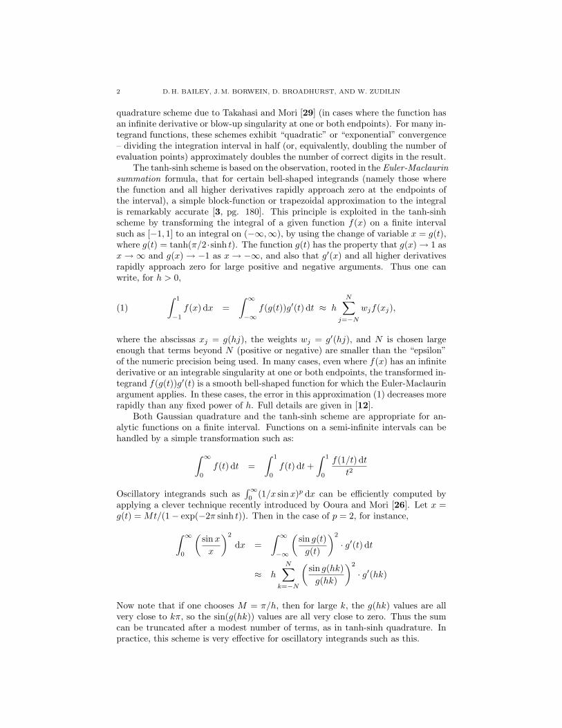
quadrature scheme due to Takahasi and Mori [29] (in cases where the function hasan infinite derivative or blow-up singularity at one or both endpoints). For many in-tegrand functions, these schemes exhibit “quadratic” or “exponential” convergence– dividing the integration interval in half (or, equivalently, doubling the number ofevaluation points) approximately doubles the number of correct digits in the result.

The tanh-sinh scheme is based on the observation, rooted in the Euler-Maclaurinsummation formula, that for certain bell-shaped integrands (namely those wherethe function and all higher derivatives rapidly approach zero at the endpoints ofthe interval), a simple block-function or trapezoidal approximation to the integralis remarkably accurate [3, pg. 180]. This principle is exploited in the tanh-sinhscheme by transforming the integral of a given function f(x) on a finite intervalsuch as [−1, 1] to an integral on (−∞,∞), by using the change of variable x = g(t),where g(t) = tanh(π/2 ·sinh t). The function g(t) has the property that g(x) → 1 asx →∞ and g(x) → −1 as x → −∞, and also that g′(x) and all higher derivativesrapidly approach zero for large positive and negative arguments. Thus one canwrite, for h > 0,

∫ 1

−1

f(x) dx =∫ ∞

−∞f(g(t))g′(t) dt ≈ h

N∑j=−N

wjf(xj),(1)

where the abscissas xj = g(hj), the weights wj = g′(hj), and N is chosen largeenough that terms beyond N (positive or negative) are smaller than the “epsilon”of the numeric precision being used. In many cases, even where f(x) has an infinitederivative or an integrable singularity at one or both endpoints, the transformed in-tegrand f(g(t))g′(t) is a smooth bell-shaped function for which the Euler-Maclaurinargument applies. In these cases, the error in this approximation (1) decreases morerapidly than any fixed power of h. Full details are given in [12].

Both Gaussian quadrature and the tanh-sinh scheme are appropriate for an-alytic functions on a finite interval. Functions on a semi-infinite intervals can behandled by a simple transformation such as:∫ ∞

0

f(t) dt =∫ 1

0

f(t) dt +∫ 1

0

f(1/t) dt

t2

Oscillatory integrands such as∫∞0

(1/x sinx)p dx can be efficiently computed byapplying a clever technique recently introduced by Ooura and Mori [26]. Let x =g(t) = Mt/(1− exp(−2π sinh t)). Then in the case of p = 2, for instance,∫ ∞

0

(sinx

x

)2

dx =∫ ∞

−∞

(sin g(t)

g(t)

)2

· g′(t) dt

≈ hN∑

k=−N

(sin g(hk)

g(hk)

)2

· g′(hk)

Now note that if one chooses M = π/h, then for large k, the g(hk) values are allvery close to kπ, so the sin(g(hk)) values are all very close to zero. Thus the sumcan be truncated after a modest number of terms, as in tanh-sinh quadrature. Inpractice, this scheme is very effective for oscillatory integrands such as this.

EXPERIMENTAL MATHEMATICS AND MATHEMATICAL PHYSICS 3

In the next four sections we consider Ising integrals, Bessel moment integrals,‘box’ integrals, and hyperbolic volumes arising from quantum field theory respec-tively. We then conclude with a description of very recent work on multidimensionalsums: Euler sums and MZVs.

2. Ising integrals

In a recent study, Bailey, Borwein and Richard Crandall applied tanh-sinhquadrature, implemented using the ARPREC package, to study the following classesof integrals [8]. The Dn integrals arise in the Ising theory of mathematical physics,and the Cn have tight connections to quantum field theory.

Cn =4n!

∫ ∞

0

· · ·∫ ∞

0

1(∑nj=1(uj + 1/uj)

)2

du1

u1· · · dun

un

Dn =4n!

∫ ∞

0

· · ·∫ ∞

0

∏i<j

(ui−uj

ui+uj

)2

(∑nj=1(uj + 1/uj)

)2

du1

u1· · · dun

un

En = 2∫ 1

0

· · ·∫ 1

0

∏1≤j<k≤n

uk − uj

uk + uj

2

dt2 dt3 · · · dtn,

where (in the last line) uk =∏k

i=1 ti.Needless to say, evaluating these n-dimensional integrals to high precision

presents a daunting computational challenge. Fortunately, in the first case, we wereable to show that the Cn integrals can be written as one-dimensional integrals:

Cn =2n

n!

∫ ∞

0

pKn0 (p) dp,

where K0 is the modified Bessel function [1]. After computing Cn to 1000-digitaccuracy for various n, we were able to identify the first few instances of Cn interms of well-known constants, e.g.,

C3 = L−3(2) =∑n≥0

(1

(3n + 1)2− 1

(3n + 2)2

)C4 =

712

ζ(3),

where ζ denotes the Riemann zeta function. When we computed Cn for fairly largen, for instance

C1024 = 0.63047350337438679612204019271087890435458707871273234 . . . ,

we found that these values rather quickly approached a limit. By using the new edi-tion of the Inverse Symbolic Calculator, available at http://ddrive.cs.dal.ca/~isc,this numerical value can be identified as

limn→∞

Cn = 2e−2γ ,

where γ is Euler’s constant. We later were able to prove this fact—this is merelythe first term of an asymptotic expansion—and thus showed that the Cn integralsare fundamental in this context [8].


The integrals Dn and En are much more difficult to evaluate, since they arenot reducible to one-dimensional integrals (as far as we can tell), but with certainsymmetry transformations and symbolic integration we were able to reduce thedimension in each case by one or two. In the case of D5 and E5, the resulting 3-Dintegrals are extremely complicated, but we were nonetheless able to numericallyevaluate these to at least 240-digit precision on a highly parallel computer system.In this way, we produced the following evaluations, all of which except the last wesubsequently were able to prove:

D2 = 1/3D3 = 8 + 4π2/3− 27 L−3(2)D4 = 4π2/9− 1/6− 7ζ(3)/2E2 = 6− 8 log 2E3 = 10− 2π2 − 8 log 2 + 32 log2 2E4 = 22− 82ζ(3)− 24 log 2 + 176 log2 2− 256(log3 2)/3 + 16π2 log 2− 22π2/3

E5?= 42− 1984 Li4(1/2) + 189π4/10− 74ζ(3)− 1272ζ(3) log 2 + 40π2 log2 2

−62π2/3 + 40(π2 log 2)/3 + 88 log4 2 + 464 log2 2− 40 log 2,

where Li denotes the polylogarithm function. In the case of D2, D3 and D4, theseare confirmations of known results. We tried but failed to recognize D5 in terms ofsimilar constants (the 500-digit numerical value is available if anyone wishes to try).The conjectured identity shown here for E5 was confirmed to 240-digit accuracy,which is 180 digits beyond the level that could reasonably be ascribed to numericalround-off error; thus we are quite confident in this result even though we do nothave a formal proof.

In a follow-on study [6], we examined the following generalization of the Cn

integrals:

Cn,k =4n!

∫ ∞

0

· · ·∫ ∞

0

1(∑nj=1(uj + 1/uj)

)k+1

du1

u1· · · dun

un.

Here we made the initially surprising discovery—now proven in [17] and in outlinemuch earlier [13]—that there are linear relations in each of the rows of this array(considered as a doubly-infinite rectangular matrix), e.g.,

0 = C3,0 − 84C3,2 + 216C3,4

0 = 2C3,1 − 69C3,3 + 135C3,5

0 = C3,2 − 24C3,4 + 40C3,6

0 = 32C3,3 − 630C3,5 + 945C3,7

0 = 125C3,4 − 2172C3,6 + 3024C3,8.

3. Bessel moment integrals

In a more recent study of Bessel moment integrals, co-authored with LarryGlasser [7], the first three authors were able to analytically recognize many ofthe Cn,k constants in the earlier study—because, remarkably, these same integralsappear naturally in quantum field theory (for odd k). We also discovered, and then


proved with considerable effort, that with cn,k normalized by Cn,k = 2n cn,k/(n! k!),we have

c3,0 =3Γ6(1/3)32π22/3

=√

3π3

8 3F2

(1/2, 1/2, 1/2

1, 1

∣∣∣∣∣14)

c3,2 =√

3π3

288 3F2

(1/2, 1/2, 1/2

2, 2

∣∣∣∣∣14)

c4,0 =π4

4

∞∑n=0

(2nn

)444n

=π4

4 4F3

(1/2, 1/2, 1/2, 1/2

1, 1, 1

∣∣∣∣∣1)

c4,2 =π4

64

[4 4F3

(1/2, 1/2, 1/2, 1/2

1, 1, 1

∣∣∣∣∣1)

−3 4F3

(1/2, 1/2, 1/2, 1/2

2, 1, 1

∣∣∣∣∣1)]

− 3π2

16,

where pFq denotes the generalized hypergeometric function [1]. The correspondingvalues for small odd second indices are c3,1 = 3L−3(2)/4, c3,3 = L−3(2)−2/3, c4,1 =7ζ(3)/8 and c4,3 = 7ζ(3)/32− 3/16.

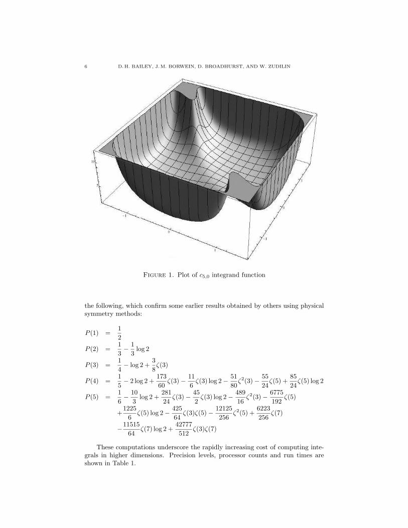
Integrals in the Bessel moment study were quite challenging to evaluate nu-merically. As one example, we sought to numerically verify the following identitythat we had derived analytically:

c5,0 =π

2

∫ π/2

−π/2

∫ π/2

−π/2

K(sin θ)K(sinφ)√cos2 θ cos2 φ + 4 sin2(θ + φ)

dθ dφ ,

where K denotes the elliptic integral of the first kind [1]. Note that this functionhas blow-up singularities on all four sides of the region of integration, with par-ticularly troublesome singularities at (π/2,−π/2) and (−π/2, π/2) (see Figure 1).Nonetheless, after making some minor substitutions, we were able to evaluate (andconfirm) this integral to 120-digit accuracy (using 240-digit working precision) in arun of 43 minutes on 1024 cores of the “Franklin” system at LBNL.

In a separate study, the first two authors studied correlation integrals for theHeisenberg spin-1/2 antiferromagnet, as given by Boos and Korepin, for a length-nspin chain [24, eqn. 2.2]:

P (n) :=πn(n+1)/2

(2πi)n·∫ ∞

−∞

∫ ∞

−∞· · ·∫ ∞

−∞U(x1 − i/2, x2 − i/2, · · · , xn − i/2)

× T (x1 − i/2, x2 − i/2, · · · , xn − i/2) dx1 dx2 · · ·dxn

where

U(x1 − i/2, x2 − i/2, · · · , xn − i/2) =

∏1≤k<j≤n sinh[π(xj − xk)]∏

1≤j≤n in coshn(πxj)

T (x1 − i/2, x2 − i/2, · · · , xn − i/2) =

∏1≤j≤n(xj − i/2)j−1(xj + i/2)n−j∏

1≤k<j≤n(xj − xk − i).

They computed numerical values for these n-fold integrals to as great a pre-cision as we could, then attempted to recognize them using pslq. They found


Figure 1. Plot of c5,0 integrand function

the following, which confirm some earlier results obtained by others using physicalsymmetry methods:

P (1) =12

P (2) =13− 1

3log 2

P (3) =14− log 2 +

38ζ(3)

P (4) =15− 2 log 2 +

17360

ζ(3)− 116

ζ(3) log 2− 5180

ζ2(3)− 5524

ζ(5) +8524

ζ(5) log 2

P (5) =16− 10

3log 2 +

28124

ζ(3)− 452

ζ(3) log 2− 48916

ζ2(3)− 6775192

ζ(5)

+1225

6ζ(5) log 2− 425

64ζ(3)ζ(5)− 12125

256ζ2(5) +

6223256

ζ(7)

−1151564

ζ(7) log 2 +42777512

ζ(3)ζ(7)

These computations underscore the rapidly increasing cost of computing inte-grals in higher dimensions. Precision levels, processor counts and run times areshown in Table 1.


n Digits Processors Run Time2 120 1 10 sec.3 120 8 55 min.4 60 64 27 min.5 30 256 39 min.6 6 256 59 hrs.

Table 1. Run times and precision levels for spin integral calculations

4. Box integrals

Let us define box integrals for dimension n as

Bn(s) :=∫ 1

0

· · ·∫ 1

0

(r21 + · · ·+ r2

n

)s/2dr1 · · ·drn

∆n(s) :=∫ 1

0

· · ·∫ 1

0

((r1 − q1)2 + · · ·+ (rn − qn)2

)s/2dr1 · · ·drn dq1 · · ·dqn.

As explained in previous treatments [4, 5], these integrals have several physicalinterpretations:

(1) Bn(1) is the expected distance of a random point from the origin (or fromany fixed vertex) of the n-cube.

(2) ∆n(1) is the expected distance between two random points of the n-cube.(3) Bn(−n + 2) is the expected electrostatic potential in an n-cube whose

origin has a unit charge. Such statements presume that electrostatic po-tential in n dimensions is V (r) = 1/rn−2, and say log r for n = 2; in otherwords, the negative powers of r can also have physical meaning.

(4) ∆n(−n + 2) is the expected electrostatic energy between two points in auniform cube of charged “jellium.”

(5) Recently integrals of this type have arisen in neuroscience e.g., the averagedistance between synapses in a mouse brain.

Note that the definitions show immediately that both ∆n(2m) and Bn(2m) arerational when m,n are natural numbers. A pivotal, original treatment on boxintegrals is the 1976 work of Anderssen et al [2]. There have been interestingmodern treatments of the Bn and related integrals, as in [10], [14, pg. 208], [32],and [30]. Related material may also be found in [23, 31].

Like the Ising integrals, some of these n-dimensional integrals are reducible to1-dimension integrals. For instance, we found that

∆3(−1) =2√π

∫ ∞

0

(−1 + e−u2+√

π u erf(u))3

u6du.

After calculating a 400-digit numerical value for this constant, we were able torecognize it as

∆3(−1) =115

(6 + 6

√2− 12

√3− 10π + 30 log(1 +

√2) + 30 log(2 +

√3))

.

A selection of results that we have found are shown in Tables 2, 3, 4 and 5.Here G denotes Catalan’s constant, namely, G :=

∑n≥0(−1)n/(2n + 1)2, θ =


n s Bn(s)any even s ≥ 0 rational, e.g.: B2(2) = 2/31 s 6= −1 1

s+1

2 −4 − 14 −

π8

2 −3 −√

22 −1 2 log(1 +

√2)

2 1 13

√2 + 1

3 log(1 +√

2)2 3 7

20

√2 + 3

20 log(1 +√

2)2 s 6= −2 2

2+s 2F1

(12 ,− s

2 ; 32 ;−1

)3 −5 − 1

6

√3− 1

12π

3 −4 − 32

√2 arctan 1√

2

3 −2 −3G + 32π log(1 +

√2) + 3 Ti2(3− 2

√2)

3 −1 − 14π + 3

2 log(2 +

√3)

3 1 14

√3− 1

24π + 12 log

(2 +

√3)

3 3 25

√3− 1

60π + 720 log

(2 +

√3)

Table 2. Recent evaluations of Box integrals

n s Bn(s)

4 −5 −√

8 arctan(

1√8

)4 −3 4 G− 12 Ti2(3− 2

√2)

4 −2 π log(2 +

√3)− 2 G− π2

8

4 −1 2 log 3− 23 G + 2 Ti2

(3− 2

√2)−√

8 arctan(

1√8

)4 1 2

5 −G10 + 3

10 Ti2(3− 2

√2)

+ log 3− 7√

210 arctan

(1√8

)5 −3 110

9 G− 10 log(2−

√3)

θ − 18 π2

−10 Cl2(

13 θ + 1

3 π)

+ 10 Cl2(

13 θ − 1

6 π)

+ 103 Cl2

(θ + 1

6 π)

+ 203 Cl2

(θ + 4

3 π)− 10

3 Cl2(θ + 5

3 π)− 20

3 Cl2(θ + 11

6 π)

5 −2 83 B5(−6)− 1

3 B5(−4) + 52 π log 3 + 10 Ti2

(13

)− 10 G

5 −1 − 11027 G + 10

3 θ log(2−

√3)

+ 148 π2

+5 log(

1+√

52

)− 5

2

√3 arctan

(1√15

)+ 10

3 Cl2(

13 θ + 1

3 π)− 10

3 Cl2(

13 θ − 1

6 π)− 10

9 Cl2(θ + 1

6 π)

− 209 Cl2

(θ + 4

3 π)

+ 109 Cl2

(θ + 5

3 π)

+ 209 Cl2

(θ + 11

6 π)

5 1 − 7781 G + 7

9 θ log(2−

√3)

+ 1360 π2 + 1

6

√5

+ 103 log

(1+√

52

)− 4

3

√3 arctan

(1√15

)+ 7

9 Cl2(

13 θ + 1

3 π)− 7

9 Cl2(

13 θ − 1

6 π)− 7

27 Cl2(θ + 1

6 π)

− 1427 Cl2

(θ + 4

3 π)

+ 727 Cl2

(θ + 5

3 π)

+ 1427 Cl2

(θ + 11

6 π)

Table 3. Recent evaluations of Box integrals, continued; here θ :=arctan

(16−3

√15

11

)


n s ∆n(s)2 −5 4

3 + 89

√2

2 −1 43 −

43

√2 + 4 log(1 +

√2)

2 1 215 + 1

15

√2 + 1

3 log(1 +√

2)

3 −7 45 −

16√

215 + 2

√3

5 + π15

3 −2 2π − 12 G + 12 Ti2(3− 2

√2)

+ 6π log(1 +

√2)

+2 log 2− 52 log 3− 8

√2 arctan

(1√2

)3 −1 2

5 −23π + 2

5

√2− 4

5

√3 + 2 log

(1 +

√2)

+ 12 log(

1+√

3√2

)− 4 log

(2 +

√3)

3 1 − 11821 −

23 π + 34

21

√2− 4

7

√3 + 2 log

(1 +

√2)

+ 8 log(

1+√

3√2

)3 3 − 1

105 −2

105 π + 73840

√2 + 1

35

√3 + 3

56 log(1 +

√2)

+ 1335 log

(1+√

3√2

)Table 4. Recent evaluations of Box integrals, continued

n s ∆n(s)4 −3 − 128

15 + 163 π − 8 log

(1 +

√2)− 32 log

(1 +

√3)

+ 16 log 2 + 20 log 3

− 85

√2 + 32

5

√3− 32

√2 arctan

(1√8

)− 96 Ti2

(3− 2

√2)

+ 32 G

4 −2 − 1615 π

√3− 8

3 π log 2 + 163 π log

(1 +

√3)− 2

3 π2 + 45 π

+ 85

√2 arctan

(2√

2)

+ 25 log 3− 4 π log

(√2− 1

)+8Ti2

(3− 2

√2)− 40

3 G− 83 log 2

4 −1 − 152315 −

815 π − 16

5 log 2 + 25 log 3 + 68

105

√2− 16

35

√3 + 4

5 log(1 +

√2)

+ 325 log

(1 +

√3)− 8

3 G + 8Ti2(3− 2

√2)− 8

5

√2 arctan

(√2/4)

4 1 − 23135 −

16315 π − 52

105 log 2 + 197420 log 3 + 73

630

√2 + 8

105

√3

+ 114 log

(1 +

√2)

+ 104105 log

(1 +

√3)

− 68105

√2 arctan

(1√8

)− 4

15 G + 45 Ti2

(3− 2

√2)

5 1 − 1279567 G− 4

189 π + 4315 π2 − 449

3465 + 323962370

√2 + 568

3465

√3− 380

6237

√5

+ 295252 log 3 + 1

54 log(1 +

√2)

+ 2063 log

(2 +

√3)

+ 64189 log

(1+√

52

)− 73

63

√2 arctan

(1√8

)− 8

21

√3 arctan

(1√15

)+ 104

63 log(2−

√3)θ

+ 57 Ti2

(3− 2

√2)

+ 10463 Cl2

(13 θ + 1

3 π)− 104

63 Cl2(

13 θ − 1

6 π)

− 104189 Cl2

(θ + 1

6 π)− 208

189 Cl2(θ + 4

3 π)

+ 104189 Cl2

(θ + 5

3 π)

+ 208189 Cl2

(θ + 11

6 π)

Table 5. Recent evaluations of Box integrals, continued

arctan((16− 3

√15)/11

), Cl denotes Clausen’s function,

Cl2(θ) =∑n≥1

sin(nθ)n2

,


and Ti denotes Lewin’s inverse-tan function,

Ti2(x) =∑n≥0

(−1)n x2n+1

(2n + 1)2.

5. Clausen functions and hyperbolic volumes

In an unpublished 1998 study [16] two of the present authors (Borwein andBroadhurst) identified 998 closed hyperbolic 3-manifolds whose volumes are ratio-nally related to Dedekind zeta values, with coprime integers a and b giving

a

bvol(M) =

(−D)3/2

(2π)2n−4

ζK(2)2ζ(2)

(2)

for a manifold M whose invariant trace field K has a single complex place, discrim-inant D, degree n, and Dedekind zeta value ζK(2). While the existence of integersa, b can be established, via algebraic K-theory as in [35], for the most part it wasand is not possible to specify the rational a/b other than empirically [35].

The simplest identity implicit in (2) devolves to

3 Cl2(α)− 3Cl2(2α) + Cl2(3α) =7√

74

L−7(2),(3)

with α = 2 arctan(√

7), as is recorded in [14, p. 91]. Here L−7(2) :=∑

n>0

(n7

)/n2

is the primitive Dirichlet L-series modulo 7 evaluated at 2 where(

n7

)is the Legendre

symbol. This was rewritten in equivalent and more self-contained form as

247√

7

∫ π/2

π/3

log

∣∣∣∣∣ tan t +√

7tan t−

√7

∣∣∣∣∣ dt = L−7(2)(4)

in [9, p. 61]—and elsewhere.Note that the integrand function of (4) has a nasty singularity at arctan(

√7)

(see Figure 2). However, we were able to numerically evaluate this integral to20,000-digit accuracy, by splitting the integral into two parts, namely on the inter-vals [π/3, arctan(

√7)] and [arctan(

√7), π/2]. Note that tanh-sinh quadrature can

be used on each part, since it can readily handle blow-up singularities at one or bothendpoints of the interval of integration. This run required 46 minutes on 1024 CPUsof the Virginia Tech Apple cluster. The right-hand side was also evaluated, usingMathematica, to 20,000-digit precision. The two values agreed to 19, 995 digits [9,pg. 61]. Alternative representations of the integral in (4) are given in [20].

We shall now provide a proof of Eqn. (3) and hence of Eqn. (4). Actually, anequivalent (if not obviously so) form of identity (3), namely

ζQ(√−7)(2) =

π2

3√

7

{A(cot

π

7

)+ A

(cot

2π

7

)+ A

(cot

4π

7

)}(5)

=2π2

7√

7

{2A(

√7) + A(

√7 + 2

√3) + A(

√7− 2

√3)}

with the notation

A(x) :=∫ x

0

11 + t2

log4

1 + t2dt = Cl2(2 arccotx),


Figure 2. Plot of integrand function in (4)

is already established in [33]. The first equality in (5) can be written as

ζQ(√−7)(2) =

π2

6L−7(2) = ζ(2) L−7(2).(6)

On noting that

cot arg√

7 + i

2√

2=

√7

cot arg(1 + i

√7)(1∓ i

√3)

4√

2=

√7± 2

√3

Cl2(θ) = Im∑n≥1

einθ

n2,

we can translate the remaining, highly non-trivial, part of (5) to

2A(√

7) + A(√

7 + 2√

3) + A(√

7− 2√

3)

= 2 Im∑n≥1

1n2

(√7 + i

2√

2

)2n

+ Im∑n≥1

1n2

((1 + i

√7)(1− i

√3)

4√

2

)2n

+Im∑n≥1

1n2

((1 + i

√7)(1 + i

√3)

4√

2

)2n

.


Now we use((1 + i

√7)(1 + i

√3)

4√

2

)2

= µe2πi/3

((1 + i

√7)(1− i

√3)

4√

2

)2

= µe−2πi/3

Im(√

7 + i

2√

2

)2n

= Im(

3 + i√

74

)n

= − Im(−µ)n for n = 0, 1, 2, . . . ,

where µ := (−3 + i√

7)/4 has absolute value 1 and arg µ = α = 2 arctan(√

7), towrite the latter equality as

2A(√

7) + A(√

7 + 2√

3) + A(√

7− 2√

3)(7)

= Im∑n≥1

µn(e2πin/3 + e−2πin/3 − 2(−1)n)n2

= Im(∑

n≥1

µn

n2−∑n≥1

µ2n

n2+

13

∑n≥1

µ3n

n2

)= Cl2(α)− Cl2(2α) +

13Cl2(3α),

where we have applied the following two standard identities

12

∑n≥1

x2n

n2=

∑n≥1

xn

n2+∑n≥1

(−1)nxn

n2

13

∑n≥1

x3n

n2=

∑n≥1

xn

n2+∑n≥1

e2πin/3xn

n2+∑n≥1

e−2πin/3xn

n2

for the dilogarithm function. It remains to substitute our finding (7) into (5) and(6) to finish a proof of identity (3).

The equivalent identity (4) can be obtained by some reasonably straightforwardbut tedious manipulation of the Clausen integral representation

Cl2(θ) = −∫ θ

0

log |2 sinσ|dσ(8)

for 0 ≤ θ < 2π, and an appropriate change of variables.

As Don Zagier points out in [33]

“we observe that the values of A(x) at algebraic arguments satisfymany non-trivial linear relations over the rational numbers; Iknow of no direct proof, for instance, of the equality of the right-hand sides of Eqns. (5) and (6).”

Zagier’s Eqns. (5) and (6) are our identity (5). Another result in [33], Theorem 3,implies the identity

ζQ(√−7)(2) =

2π2

21√

7

{3A

(1√7

)+ 3A

(3√7

)+ A

(5√7

)},(9)


which may be thought of as complimentary to Eqn. (5) (see pg. 300 in [33] fordetails). Since

A

(1√7

)= Cl2

(2 arctan

√7)

A

(3√7

)= Cl2

(2 arctan

√7

3

)A

(5√7

)= Cl2

(2 arctan

√7

5

),

and

2 arctan√

7 = α, 2 arctan√

73

= −2α + 2π, 2 arctan√

75

= 3α− 2π,

identity (3) follows from (9) immediately. Thus paper [33] contains two differentproofs of (3)!

Let us clarify the current status and somewhat-complicated history of variousof the discoveries in [16]. Until recently the authors of [16] after discussion withZagier believed (5) to be unproven. It was only when Zudilin spent time with DonZagier in 2008 that he remembered his equivalent pre-dilogarithm (see [34, 35])result in [33]. Two of the present authors (Borwein and Broadhurst) [16] wrote

“While the existence of such relations is understood [33, 34, 35],their precise forms appear to be unpredictable, thus far, by de-ductive mathematics. They are therefore ripe for the applicationof experimental mathematics.”

The great bulk of the results recorded in [16] remain unproven. They were dis-covered by intensive physically and mathematically motivated computation, usingSnapPea, Pari-GP, Maple, and other tools.

Indeed, the casesD = −8,−11,−15,−20,−24

are challenging enough! These five respectively yield the following conjecturedidentities—each of which is open. First

27Cl2(θ2)− 9Cl2(2θ2) + Cl2(3θ2)?= 8Cl2

(2π

8

)+ 8Cl2

(6π

8

),(10)

with θ2 := 2 arctan√

2. Secondly,

15Cl2(θ11)− 10Cl2(2θ11) + Cl2(5θ11)?= 11

5∑k=1

(k

11

)Cl2

(2πk

11

),(11)

where θ11 := 2 arctan√

11 and(

k11

)is the Jacobi (or Legendre) symbol for the

Dirichlet character. Thirdly,

(12) 24Cl2(θ5,3)− 12Cl2(2θ5,3)− 8Cl2(3θ5,3) + 6Cl2(4θ5,3)

?= 157∑

k=1

(k

15

)Cl2

(2πk

15

),


with θ5,3 := 2 arctan√

5/3. Fourthly

(13) 36Cl2(θ5)− 30Cl2(2θ5) + 4Cl2(3θ5) + 3Cl2(4θ5)

?= 20∑

k∈{1,3,7,9}

Cl2

(2πk

20

),

with θ5 := 2 arctan√

5. Finally,

(14) 60Cl2(θ3,2)− 18Cl2(2θ3,2)− 4Cl2(3θ3,2) + 3Cl2(4θ3,2)

?= 24∑

k∈{1,5,7,11}

Cl2

(2πk

24

),

with θ3,2 := 2 arctan√

3/2. So, for the fifth time, we have a relation that is aseasy to check numerically as it appears hard to derive. Needless to say, it wouldbe interesting to check whether Zagier’s 1986 theorems in [33] work for all suchsmall values of D; Theorem 2 in [33] looks sufficiently powerful for this task, whileTheorem 3 therein depends critically on a delicate geometric construction and mightbe of use for D = −11,−15,−20. Moreover, is there a more transparent method todeduce identity (3) as well as (10)–(14)?

As another example of the ubiquity of Clausen values, we complete this sectionwith the most difficult integral evaluation required in [5]:

K1 :=∫ 4

3

arcsec (x)√x2 − 4 x + 3

dx(15)

= 3Cl2

(θ

3

)− 3

11Cl2

(θ

3− π

6

)− 3

11Cl2

(θ

3+

π

6

)+

1811

Cl2(θ − π

3

)−15

11Cl2

(θ − 2π

3

)− 3

11Cl2

(θ +

π

6

)− 3

11Cl2

(θ − π

6

)+(2 θ − π

2

)log(2−

√3)

.

Here

θ := arctan

(16− 3

√15

11

).

It may well be that this closed form (15) for K1 can be further simplified.

6. Relations between MZVs and Euler sums

We conclude with an application of experimental mathematics to discover re-lations between multiple zeta values (MZVs) of the form

ζ(s1, s2, . . . , sk) =∑

n1>n2>...>nk>0

1ns1

1 . . . nsk

k

with weight w =∑k

i=1 si and depth k and Euler sums of the more general form∑n1>n2>...>nk>0

εn11 . . . εnk

k

ns11 . . . nsk

k


with signs εi = ±1. Both types of sum occur in evaluations of Feynman diagramsin quantum field theory [18, 19] as mentioned in [14]. These sums are describedin some mathematical detail in [15, Chapter 3].

First we recall the first Broadhurst–Kreimer conjectures (see [18] and also [15])for the enumeration of primitive MZVs and Euler sums of a given weight and depth.Let En,k be the number of independent Euler sums at weight n > 2 and depth kthat cannot be reduced to primitive Euler sums of lesser depth and their products.It is conjectured that [18]∏

n>2

∏k>0

(1− xnyk)En,k?= 1− x3y

(1− xy)(1− x2).

We emphasise that, since the irrationality of odd values of depth-one MZVs(i.e., Riemann’s ζ) is not settled, such dimensionality conjectures are necessarilyexperimental. Now let Dn,k be the number of independent MZVs at weight n > 2and depth k that cannot be reduced to primitive MZVs of lesser depth and theirproducts. Thus we believe that D12,4 = 1, since there is no known relationshipbetween the depth-4 sum ζ(6, 4, 1, 1) =

∑j>k>l>m 1/(j6k4lm) and MZVs of lesser

depth or their products. It is conjectured that [18]∏n>2

∏k>0

(1− xnyk)Dn,k?= 1− x3y

1− x2+

x12y2(1− y2)(1− x4)(1− x6)

.

The final Broadhurst–Kreimer conjecture concerns the existence of relationsbetween MZVs and Euler sums of lesser depth. The now proven relation [19]

ζ(6, 4, 1, 1) =649

ζ(9, 3) +371144

ζ(9, 3) + 3ζ(2)ζ(7, 3) +10724

ζ(5)ζ(7)

+112

ζ4(3)− 3131144

ζ(3)ζ(9) +72ζ(2)ζ2(5) + 10ζ(2)ζ(3)ζ(7)

+ζ2(2)[35ζ(5, 3)− 1

5ζ(3)ζ(5)− 18

35ζ(2)ζ2(3)− 117713

2627625ζ4(2)

]shows that the depth-4 MZV on the left can be expressed in terms of Euler sums oflesser depth and their products. In fact, it suffices to include the alternating doublesum ζ(9, 3) =

∑j>k>0(−1)j+k/(j9k3), where a bar above an argument of ζ serves

to indicate an alternating sign. In the language of [18, 19] this is a “pushdown”,at weight 12, of an MZV of depth 4 to an Euler sum of depth 2. Let Mn,k bethe number of primitive Euler sums of weight n > 2 and depth k whose productsfurnish a basis for all MZVs. It is conjectured that [18]∏

n>2

∏k>0

(1− xnyk)Mn,k?= 1− x3y

1− x2.

Then by comparison of the output D21,3 = 6, D21,5 = 9, D21,7 = 1 of (16) with theoutput M21,3 = 9, M21,5 = 7 of (16) we conclude that at weight 21, for example,three pushdowns are expected from depth 5 to depth 3 and one from depth 7 todepth 5.

By massive use of the computer algebra language form, to implement theshuffle algebras of MZVs and Euler sums, the authors of [19] were recently able toreduce all Euler sums with weight w ≤ 12 and all MZVs with w ≤ 22 to concretebases whose sizes are in precise agreement with conjectures (16,16). Moreover,


further support to these conjectures came by studying even greater weights, w ≤ 30,using modular arithmetic. However, such algebraic methods were insufficient toinvestigate pushdown at weight 21. Instead the authors resorted to a combinationof the pslq methods reported in [11] with the lll algorithm [25] of Pari-GP [27],finding empirical forms for precisely the expected numbers of pushdowns at allweights w ≤ 21. Most notable of these is the pushdown from depth 7 to depth 5,at weight 21, in the empirical form

ζ(6, 2, 3, 3, 5, 1, 1) ?= −32681

ζ(3, 6, 3, 6, 3) + {depth− 5 MZV products}

where the remaining 150 terms are formed by MZVs with depth no greater than 5,and their products.

It is proven, by exhaustion, in [19] that the shuffle algebras do not allow thesum ζ(6, 2, 3, 3, 5, 1, 1) in equation (16) to be reduced to MZVs of depth less than7. It is also proven that all other MZVs of weight 21 and depth 7 are reducible toζ(6, 2, 3, 3, 5, 1, 1) and MZVs of depth less than 7. Yet it appears to be far beyondthe limits of current algebraic methods to prove that inclusion of the rather strikingdepth-5 alternating sum

ζ(3, 6, 3, 6, 3) =∑

j>k>l>m>n>0

(−1)k+m

(jk2lm2n)3,

with the rather simple coefficient −326/81, leaves the remainder reducible to MZVsof depth no greater than five.

Thus we are left with a notable empirical validation of a pushdown conjecturerelevant to quantum field theory, crying out for elucidation.

7. Conclusion

We have presented here a brief survey of the rapidly expanding applicationsof experimental mathematics (in particular, the application of high-precision arith-metic) in mathematical physics. It is worth noting that all but the penultimate ofthese examples have arisen in the past five to ten years. Efforts to analyze inte-grals that arise in mathematical physics have underscored the need for significantlyfaster schemes to produce high-precision values of 2-D, 3-D and higher-dimensionalintegrals. Along this line, the “sparse grid” methodology has some promise [28, 36].

Current research is aimed at evaluating such techniques for high-precision ap-plications. To illustrate the difficulty, we leave as a challenge to the reader thecomputation of the triple integral∫

C

√f(u, v, w)− 2 du dv dw = 1.1871875 . . . ,

where C := [0, 1/2]3 and

f(u, v, w) := cos2 ((v + w)π) + cos2 ((u− v)π) + cos2 ((u + w)π)+ cos2 (vπ) + cos2 (uπ) + cos2 (wπ)

to, say, 32 decimal digit accuracy.


References

[1] Milton Abramowitz and Irene A. Stegun, ed., Handbook of Mathematical Functions, Dover,New York, 1972.

[2] R. Anderssen, R. Brent, D. Daley, and P. Moran, “ConcerningR 10 · · ·

R 10 (x2

1 + · · · x2n)

12 dx1 · · · dxn and a Taylor series method,” SIAM Journal of Applied

Mathematics, vol. 30 (1976), 22–30.

[3] Kendall E. Atkinson, Elementary Numerical Analysis, John Wiley, 1993.

[4] David H. Bailey, Jonathan M. Borwein and Richard E. Crandall, “Box integrals,” Journalof Computational and Applied Mathematics, vol. 206 (2007), 196–208.

[5] David H. Bailey, Jonathan M. Borwein and Richard E. Crandall, “Advances in the Theoryof Box Integrals,” to appear in Mathematics of Computation; available at

http://crd.lbl.gov/~dhbailey/dhbpapers/BoxII.pdf.

[6] David H. Bailey, David Borwein, Jonathan M. Borwein and Richard Crandall,“Hypergeometric forms for Ising-class integrals,” Experimental Mathematics, vol. 16 (2007),

no. 3, 257–276.

[7] David H. Bailey, Jonathan M. Borwein, David Broadhurst and M. L. Glasser, “Ellipticintegral evaluations of Bessel moments,” Journal of Physics A: Mathematics and General,

vol. 41 (2008), 205203.

[8] David H. Bailey, Jonathan M. Borwein and Richard E. Crandall, “Integrals of the Isingclass,” Journal of Physics A: Mathematics and General, vol. 39 (2006), 12271–12302.

[9] David H. Bailey, Jonathan M. Borwein, Neil Calkin, Roland Girgensohn, Russell Luke and

Victor Moll, Experimental Mathematics in Action, A. K. Peters, Wellesley, MA, 2007.[10] David H. Bailey, Jonathan M. Borwein, Vishaal Kapoor, and Eric W. Weisstein, “Ten

problems in experimental mathematics,” American Mathematical Monthly, vol. 113 (2006),481–509.

[11] D. H. Bailey and D. Broadhurst, “Parallel integer relation detection: Techniques and

applications,” Mathematics of Computation, vol. 70, no. 236 (2000), 1719–1736.[12] D. H. Bailey, X. S. Li and K. Jeyabalan, “A comparison of three high-precision quadrature

schemes,” Experimental Mathematics, vol. 14 (2005), 317–329.

[13] P. Barrucand, “Sur la somme des puissances des coefficients multinomiaux et les puissancessuccessives d’une fonction de Bessel,” Comptes rendus hebdomadaires des seances de

l’Academie des sciences, vol. 258 (1964), 5318–5320.

[14] Jonathan M. Borwein and David H. Bailey, Mathematics by Experiment: PlausibleReasoning in the 21st Century, A. K. Peters, Natick, MA, second edition, 2008.

[15] Jonathan M. Borwein, David H. Bailey and Roland Girgensohn, Experimentation in

Mathematics: Computational Routes to Discovery, A. K. Peters, Natick, MA, 2004.[16] J. M. Borwein and D. J. Broadhurst, “Determinations of rational Dedekind-zeta invariants

of hyperbolic manifolds and Feynman knots and links,” [arXiv:hep-th/9811173], 19November 1998.

[17] Jonathan M. Borwein and Bruno Salvy, “A proof of a recursion for Bessel moments,”

Experimental Mathematics, vol. 17 (2008), 223–230.[18] D. J. Broadhurst and D. Kreimer, Association of multiple zeta values with positive knots

via Feynman diagrams up to 9 loops, Phys. Lett. B 393 (1997) 403–412,

[arXiv:hep-th/9609128].[19] J. Blumlein, D. J. Broadhurst and J. A. M. Vermaseren, The Multiple Zeta Value Data

Mine, [arXiv:math-ph/09072557].[20] Mark W. Coffey, “Alternative evaluation of a ln tan integral arising in quantum field

theory,” [arXiv:0810.5077], November 2008.

[21] Helaman R. P. Ferguson, David H. Bailey and Stephen Arno, “Analysis of PSLQ, an integer

relation finding algorithm,” Mathematics of Computation, vol. 68, no. 225 (Jan 1999),351–369.

[22] J. A. M. Vermaseren, New features of FORM, [arXiv:math-ph/0010025].[23] Wolfram Koepf, Hypergeometric Summation: An Algorithmic Approach to Summation and

Special Function Identities, American Mathematical Society, Providence, RI, 1998.

[24] H. Boos and V. Korepin, “Evaluation of integrals representing correlations in the XXXHeisenberg spin chain,” in: MathPhys Odyssey, 2001, Prog. Math. Phys., vol. 23,

Birkhauser, Boston, 2002, 65–108.


[25] A. K. Lenstra, H. W. Lenstra and L. Lovasz, Factoring Polynomials with Rational

Coefficients, Math. Ann. 261 (1982) 515-534.

[26] T. Ooura and M. Mori, “Double exponential formulas for oscillatory functions over the halfinfinite interval,” Journal of Computational and Applied Mathematics, vol. 38 (1991),

353–360.

[27] The PARI/GP page: http://pari.math.u-bordeaux.fr/

[28] S. Smolyak, “Quadrature and interpolation formulas for tensor products of certain classes of

functions,” Soviet Math. Dokl., vol. 4 (1963), 240243.

[29] H. Takahasi and M. Mori, “Double exponential formulas for numerical integration,”Publications of RIMS, Kyoto University, vol. 9 (1974), pg. 721–741.

[30] Michael Trott, Private communication, 2005.

[31] Michael Trott, “The area of a random triangle,” Mathematica Journal, vol. 7 (1998),189–198.

[32] Eric Weisstein, “Hypercube line picking,” available athttp://mathworld.wolfram.com/HypercubeLinePicking.html.

[33] D. Zagier, “Hyperbolic manifolds and special values of Dedekind zeta-functions,” Invent.

Math., vol. 83 (1986), 285–301.[34] D. Zagier,“The remarkable dilogarithm,” J. Math. Phys. Sci., vol. 22 (1988), 131–145.

[35] D. Zagier, “Polylogarithms, Dedekind zeta functions and the algebraic K-theory of fields,”

in: Arithmetic algebraic geometry (Texel, 1989), Progr. Math., vol. 89, Birkhauser, Boston,1991, 391–430.

[36] C. Zenger, “Sparse grids,” in W. Hackbusch, ed., Parallel Algorithms for Partial

Differential Equations, vol. 31 of Notes on Numerical Fluid Mechanics, Vieweg, 1991.

D.H. Bailey: Lawrence Berkeley National Laboratory, Berkeley, CA 94720E-mail address: [email protected]

J.M. Borwein: School of Mathematical and Physical Sciences, University ofNewcastle, Callaghan, NSW 2308, Australia

E-mail address: [email protected]

D. Broadhurst: Physics and Astronomy Department, Open University, Milton Keynes

MK7 6AA, UK

E-mail address: [email protected]

W. Zudilin: School of Mathematical and Physical Sciences, University of Newcastle,

Callaghan, NSW 2308, AustraliaE-mail address: [email protected]

Experimental Mathematics and Mathematical Physics · Experimental Mathematics and Mathematical Physics David H. Bailey, Jonathan M. Borwein, David Broadhurst, and Wadim Zudilin Abstract.

Documents