Experimental Evaluation of Methods for Characterization of ...

EXPERIMENTAL EVALUATION OF METHODS FOR CHARACTERIZATION OF POWER OUTPUT OF HIGH POWER ULTRASONIC TRANSDUCERS

David Grewell*, Karl Graff**, Avraham Benatar* * The Ohio State University **Edison Welding Institute

Abstract

This paper reviews the evaluation of different techniques used to characterize the power output of high power ultrasonic transducers. Three laboratory measurement techniques were studied: 1) electrical, 2) calorimetric and 3) mechanical transmission line. The loads were theoretically modeled and their thermal, mechanical, and electrical losses were identified. It was found that the most accurate power measurement was based on multiplication of the measured voltage and current without the use of filters or methods that attempt to differentiate between stored and dissipated energy.

Introduction The report reviews the evaluation of three techniques used to characterize ultrasonic transducers:

• Electrical, • Calorimetric, • Mechanical transmission line.

The study was conducted to determine which oif any techniques provide an accurate measurement of power dissipation and efficiency, of standard ultrasonic transducers. While the study only evaluated piezoelectric transducers, it is believed that the results are applicable to other types of transducers.

Ultrasonic transducers Ultrasonic transducers are often referred to as motors, since they convert electrical energy into mechanical energy. The mechanical energy is transmitted through vibrational displacements at the front of the transducer. While the design, construction, and even operation vary significantly between transducers, they are typically characterized in terms of:

1. Maximum power output, 2. Output displacement, 3. Frequency, 4. Efficiency.

Currently, there are no widely accepted standard methods for measuring many of the characteristic values. For example, the maximum power output can be measured and defined in terms of transient peak power or at 100% condition duty cycle. Also, the loading condition can affect the outcome of the measurements. If the load is

water, or a thermoplastic, or rubber the outcome of the measurement can greatly vary.

Wave propagation A wave traveling to the right (forward traveling wave) along with a reflected fraction can also be defined as shown in Eq. 1[1, 2]. In this case, the peak amplitude of the wave is defined as A, the time and position of the observer of the wave are defined as t (time) and x (x-position) respectively, and k is the wave number:

)cos()sin()()sin()cos()(),( wtkxfAwtkxfAtxy −−+= 11 ( 1) Where f is defined as the fraction of the wave reflected [2]. Herbertz [3] used these equations to propose that by simply measuring the displacement of a transmission rod at selected points it would be possible to determine the transmitted and reflected wave, and thus determine the dissipated energy. With his theory it is shown that the power dissipated (Pl) at a load is defined by Eq, 2 for the energy passing through a transmission line.

)(2

1 22

21 vvcAPl −= ρ (2)

In Eq. 2, ρ is the density of the transmission line, c is the velocity of sound in the transmission line, and A is the cross sectional area of the transmission line. In addition, v1 is the amplitude of the velocity at a point generated by the transmitted wave, and v2 is velocity at a point generated by the reflected wave. By using the mechanical transmission line method, there could be a phase difference (a) between the two waves (v1, v2) and that each would have a particular phase (a1, a2). Then, by using Eq. 1, it is possible to define the velocity at any point in the transmission line as:

)sin()sin(),( 2211 kxawtvkxawtvtxv +++−+= (3)

Thus, by measuring the velocity (v) of a transmission rod at different times and locations it is possible to calculate the power dissipated at the end of the transmission rod.

Losses There are two primary losses in the system: mechanical (hysteresis heating), and dielectric, and Ohmic. It is interesting to note that the mechanical losses are relatively load- independent. However, the dielectric losses for the

transducers and transformers are not load-independent. For piezoelectric transducers it is possible to estimate the losses [4].

(W) VPavg22 Eeffo "επωε= (4)

where ”eff is the effective dielectric loss which is both frequency and temperature dependent and V is the total volume of material between the electrodes. In Eq. 4, E is the electric field density. Thus, it can be seen that the dielectric losses are load (E, electric field density) dependent. The losses in the transformer and magnostrective transducers can be estimated by measuring the current and impendence and simply using Ohmic losses.

Calorimeter Historically, the calorimeter has been used to measure energy dissipation in many fields, from chemistry to mechanical impact studies, such as ballistics. The theory of the calorimeter is simple. By measuring the thermal energy in a system in the initial condition (initial temperature To) and measuring the energy in the final condition (final temperature Tf), it is possible to measure the energy dissipated into the system if the thermal losses (usually minimized to be negligible) and the thermal properties [(namely specific heat(c])) are known. By using heat balance equations it is possible to derive the widely used Eq. 5, to calculate the total energy dissipated (Q) within a load of known mass (m =(volume x ρ )) and density (ρ).

)( of TTmcQ −= (5)

Experimentation

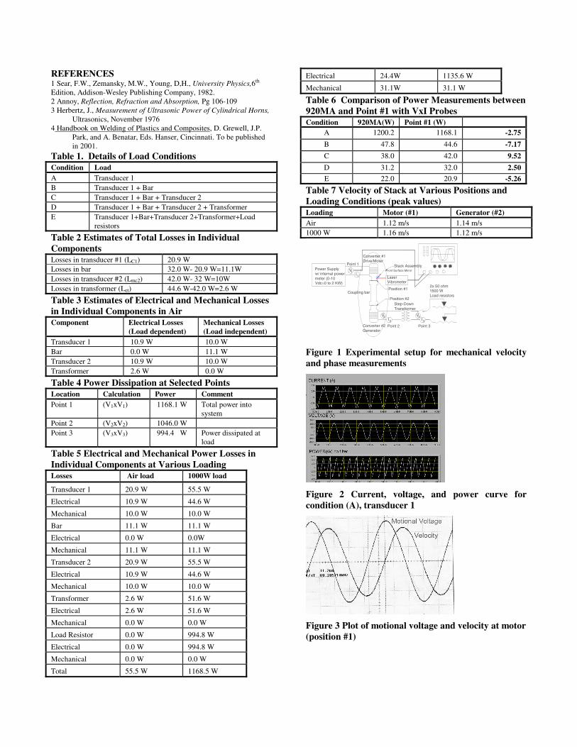
Experiments were set up to measure the power delivered from the power supply (Pin), power losses within the system (Pl), and power dissipated (Pd) within a load. An electrical/mechanical representation of the experimental setup is shown in Figure 1. This setup is analogous to a motor/generator setup in that one transducer converter electrical energy in to mechanical energy. This mechanical energy is transmitted through a coupling bar to the opposite transducer. Thus, this setup is often referred to as a “back-to-back” load. It should be noted that the load resistors, couple bar, and transducers were cooled with compressed air to prevent over-heating. It is important to note that while Figure 1 shows three voltage and current meters, the experimental setup only allowed one voltage and current meter. Thus, the meters were repositioned for different experiments as needed.

Electrical power measurements

In order to determine the losses of all components, the power delivered (Pin) from the power supply (V1 x I1) was measured for each component using the sequence shown in Table 1. It is important to note that for all cases, except E, the load was relatively low (<50 W) and is referred to as an “air-load”. In addition to these tests, power measurements were recorded at all three points (P1, P2 and P3) under ~1000 W of loading. This permitted the losses of the transducers and bar (LS, stack losses where the stack is defined as the transducers and coupling bar assembly) as well as the transformer losses (LT) to be estimated under load. The following power balance formulae were used:

LS= P1 – P2 & LT= P3 – P2 (6) In the case of the stack assembly, there are three separate components with individual losses. In fact, the two transducers have both electrical losses and mechanical losses due to hysteresis losses as detailed previously. Thus, in order to measure the dielectric losses of the transducer, the power measurements were recorded at the power levels of interest (in air and at ~ 1,000W).

Calorimetric study The experimental setup used in this study was consistent with standard calorimetric setups. A horn machined from titanium, which has a relatively low thermal conductivity, was selected in order to reduce thermal conduction into the horn, to minimize experimental error. The face of the horn measured 50 mm x 32 mm in dimensions. Three 36-gage thermal couples were submersed into the water bath and the temperature was recorded using a PC-based data acquisition at a sampling rate of 1 Hz. The load was varied by using varying amounts of water; 250, 500 and 750 ml of water. Both tap water and distilled water were used. The horn was extended to a constant distance into the container, so that the height of the water against the horn increased with increased amounts of water. The power into the system was measured using the internal power meter on the 920MA (0-10 VDC corresponds to 0 to 2,000 W). This signal was recorded and integrated using the Yokogawa DL1540L oscilloscope. The ultrasonic energy was applied for varying lengths of time; 2.5, 5, 10 and 15 s. In order to account for the losses of the system, the “in air” (80 W) was subtracted from the measured value. Mechanical transmission line power measurements In order to determine the proper velocities of the forward and reflected waves with the coupling bar, or transmission

line, the velocity of the displacement was measured at two locations (Position #1 and Position #2). These locations are detailed in Figure 1. These locations were selected because they provided surfaces parallel to the displacement, which allowed the laser vibrometer (model PolyTec OFV 1002) to make an accurate measurement. The voltage to the transducer was also recorded and was used as a reference, in order to calculate the phase difference between (a1 –a2), the forward and reflected wave.

Results Electrical power measurements

This section details the results of the electrical measurements of this experiment. It is important to note that there are two loading conditions, in air (minimal load) and loaded (approximately 1,000 W).

In air (no load) power losses Figure 2 shows the resulting VxI and power curves for the system under condition A (Table 1). It is interesting to note that the current has a harmonic wave current of the 60 kHz wave form imposed on to it. This stored energy does not dissipate energy and thus, in order to accurately calculate the power, the instantaneous product of the voltage and current was calculated and the average value recorded as the average power over a multiple of waveforms. Table 2 details the losses for the in-air conditions (low load). It is important to note that some of the mechanical losses are load independent as long as frequency and strain (amplitude) are constant. Thus, the mechanical loss for transducers at 20,000 Hz and 20 µm is 10 W, because in condition C, the electrical connection across the piezoelectric disc of Transducer 2 are open and thus there is no current and thus no dielectric loss. That is to say, the loss for Transducer 2 is purely mechanical (Lmc2). If Transducer 1 and 2 are relatively identical, it is possible to estimate the loss for Transducer 1. For example, it can be assumed that in this condition (air-loading), the mechanical loss for Transducer 1 is 10 W and thus the dielectric loss for Transducer 1 (Lec1) is defined as: LC1 =Total Losses in Transducer 1= Lec1 + Lmc1 (7) Therefore: Lec1 = LC1 - Lmc1= 20.9 W - 10 W = 10.9 W (8) Thus, in summary it is possible to estimate the losses of the individual components as seen in Table 3.

Loaded power losses

With the load attached, (load resistors R = 89.6 Ohm and L = 86.6 µH), Table 4 summarizes the power dissipation at various locations. Based on these data, there are several additional losses, which can be calculated in the system. For example, the electrical loss in the transformer (LeT) at ~ 1,000 W loading, which is equal to its total loss (LT =LeT), is defined as: (V2xI2) - (V3xI3)=1,046.0W - 994.4W =51.6W ( 9) In addition, the loss in stack is: (V1xI2) - (V2xI2 )=1,168.1W-1,046.0 W =122.1 W (10) Assuming that the losses in the two transducers are the same, then it is possible to estimate the losses in all the components as shown in Table 5.

Comparison of power readings For comparison, the power readings from the Branson 920MA were compared to the power measurements made at Point #1. It should be noted that the 920MA power meter has a filter that removes the harmonic sub-components and an analog multiplier. This allows the real power component to be calculated. As seen in Table 6, the results are very similar; differing by only a few percentage points or Watts, especially once an appreciable load is applied to the system (~1,000 W). Thus, it is assumed that the power meter within the 920MA is accurate at moderate loads (~1,000 W). Mechanical transmission line power measurements The measured velocities at Points #1 and #2 (Figure 1) are detailed in Table 7. It is seen that at the motor position (position #1), there is a slight increase in the velocity (displacement) when then load goes from air to 1,000 W. The increase is 3.6 %, which is within the amplitude regulation of the manufacturer. In addition, the amplitude at the generator side increases, but only by 2.0 %. Thus, in order to obtain the real loss in amplitude through the bar under load, it is assumed that the gain of the coupling bar is (1:1.14/1.12) or 1.02. Hence, the theoretical velocity at position #2, under load (1,000 W) is 1.16 m/s x 1.02, or 1.18 m/s. Comparing this to the measured value, 1.12 m/s, there is a 5.4 % difference. Since this difference is significant, it is assumed that this is due to the super-positioning of the transmitted and reflected waves. At this point, one may try to use this difference of velocity in transmission line power equation (v1

2 - v22), however it is important to note that the

measured velocities are not the velocities of the transmitted and reflected wave, but are simply the velocity of the two waves superimposed on each other at different locations (x =0 and x =0.2545 m so that sin(kx )=1). Thus, in order to determine the actual values of v1 and v2, the phase (a) change of the super-positioned waves were calculated. This was estimated by measuring the velocities at position #1 and #2 and the motional voltage to the transducer, (Figure 1). To estimate the phase change (a), 180 deg (2π(rad), 10.3 µs) is added to the velocity measurement at position #1 (motor).giving Thus, the various phase shifts are shown below: am(position #1) = 11.2 µs

ag(position #1) = 10.3 µs a = am- ag = 0.9 µs = 6.5 deg or 0.133 rad

ThusFurther, by setting a1 to zero (0) in transmission line equation it is possible to set a2 to 0.133 rad. Thus, based on transmission line equation, it is possible to define the superimposed velocities (measured) at two locations (x =0 and x =0.2545 m) as seen below:

smwtvwtvtvg

/.)..sin().sin(),.(

121283096113028396025450

21

=+++−+=

(11)

smwtvwtvtvm /.).sin(

)sin(),(16101130

0002

1 =−++−+=

(12)

If a time is selected so that the functions are based on a multiple of cycles, (t = πn/2ω, n = any integer >1) it is possible to reduce the above equations to give,

)9936.0(/16.1 & )9936.0(/12.1 2121 vvsmvvsm +=+= (13)

It is seen that there is no solution for v1 and v2 that satisfies Eq. 13. Thus, while an attempt was made during these experiments to determine the power (~1,000 W) transmitted through the coupling bar, these experiments did not provide the required information. Thus, it is left to future investigations to determine the proper methodology for measuring transmitted power through a transmission line via the Herbertz proposal.

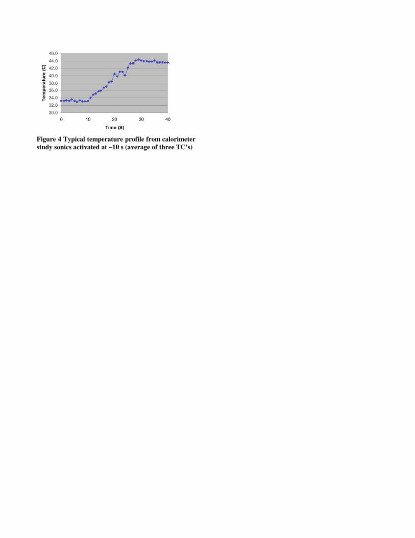
Calorimetric study Figure 4 shows a typical temperature profile from the calorimetric study. It is important to note that in this figure the average of the three separate thermocouples is shown. As expected there is a gradual and nearly linear increase in temperature while the ultrasonic energy is applied. This is important to note, since a linear relationship indicates there areis insignificant thermal losses. This is also seen in the fact that once the ultrasonic energy is discontinued (> 30 s), there is little change in the temperature. Thus, the assumption that one

can neglect heat loss into the horn and bath container is appropriate. In this experiment, the average power dissipated, as measured from the electronic power meter, was 1,228 W. By evaluating the slope (dT/dt) of the temperature profile (0.611 C/s), the average thermal power dissipated was 1,280 W. Thus the experimental error was 4.25 %. In the studies in which the experimental error was evaluated as a function of power dissipation level (S), it was seen that high power levels greatly reduced the experimental error. The experimental error was less than 2 %, once the power exceeded approximately 800 W. If the noise (N) of the signal is assumed to be the “in-air-power” dissipation (80 W) of the system, it can be estimated that the signal to noise ratio (S/N) should be greater than 10. In those experiments that evaluated experimental error as a function of exposure time, it was found that for a time span of less than 5 to 7 s, the experimental error was relatively large (> 20 %). This is due to the fact that at these short exposure times, the increase in the water temperature was relatively small (< 2 ºC) and the accuracy of the temperature measurement was critical. In the experiments in which tap water, distilled water, and de-gassed distilled water were compared, the results showed no significant difference. If the time was greater than 10 s, the difference was 2-5 %.

Conclusions The primary results of this study include: 1. The most accurate electrical power measurements are

based on real time multiplications of voltage and current over a multiple of cycles (AC wave current)

2. Calorimetric techniques can be used to accurately measure ultrasonic energy dissipation (5 % accuracy)

3. It was not possible to determine the proper methodology for measuring mechanical energy transmission through a line by measuring the velocity and phase shifts at two locations.

4. The power meter in the 920MA is accurate to within 3 % at relatively high loads (1,000 W).

5. The so-called “back-to-back” load allows accurate (within 3 %) power measurements to be made for ultrasonic loads.

6. Distilled, tap, and degassed water all behaved similarly as loads with similar power dissipation estimates.

Acknowledgements

Special thanks to Branson Ultrasonics Corp., City/Country, for all their help and support. Special thanks are extended to Mike Schmeer and Allan Roberts for their assistance.

REFERENCES 1 Sear, F.W., Zemansky, M.W., Young, D,H., University Physics,6th Edition, Addison-Wesley Publishing Company, 1982. 2 Annoy, Reflection, Refraction and Absorption, Pg 106-109 3 Herbertz, J., Measurement of Ultrasonic Power of Cylindrical Horns,

Ultrasonics, November 1976 4 Handbook on Welding of Plastics and Composites, D. Grewell, J.P.

Park, and A. Benatar, Eds. Hanser, Cincinnati. To be published in 2001.

Table 1. Details of Load Conditions Condition Load A Transducer 1 B Transducer 1 + Bar C Transducer 1 + Bar + Transducer 2 D Transducer 1 + Bar + Transducer 2 + Transformer E Transducer 1+Bar+Transducer 2+Transformer+Load

resistors

Table 2 Estimates of Total Losses in Individual Components Losses in transducer #1 (LC1) 20.9 W Losses in bar 32.0 W- 20.9 W=11.1W Losses in transducer #2 (Lmc2) 42.0 W- 32 W=10W Losses in transformer (Let) 44.6 W-42.0 W=2.6 W

Table 3 Estimates of Electrical and Mechanical Losses in Individual Components in Air Component Electrical Losses

(Load dependent) Mechanical Losses (Load independent)

Transducer 1 10.9 W 10.0 W Bar 0.0 W 11.1 W Transducer 2 10.9 W 10.0 W Transformer 2.6 W 0.0 W

Table 4 Power Dissipation at Selected Points Location Calculation Power Comment Point 1 (V1xV1) 1168.1 W Total power into

system Point 2 (V2xV2) 1046.0 W Point 3 (V3xV3) 994.4 W Power dissipated at

load

Table 5 Electrical and Mechanical Power Losses in Individual Components at Various Loading Losses Air load 1000W load

Transducer 1 20.9 W 55.5 W

Electrical 10.9 W 44.6 W

Mechanical 10.0 W 10.0 W

Bar 11.1 W 11.1 W

Electrical 0.0 W 0.0W

Mechanical 11.1 W 11.1 W

Transducer 2 20.9 W 55.5 W

Electrical 10.9 W 44.6 W

Mechanical 10.0 W 10.0 W

Transformer 2.6 W 51.6 W

Electrical 2.6 W 51.6 W

Mechanical 0.0 W 0.0 W

Load Resistor 0.0 W 994.8 W

Electrical 0.0 W 994.8 W

Mechanical 0.0 W 0.0 W

Total 55.5 W 1168.5 W

Electrical 24.4W 1135.6 W

Mechanical 31.1W 31.1 W

Table 6 Comparison of Power Measurements between 920MA and Point #1 with VxI Probes Condition 920MA(W) Point #1 (W)

A 1200.2 1168.1 -2.75

B 47.8 44.6 -7.17

C 38.0 42.0 9.52

D 31.2 32.0 2.50

E 22.0 20.9 -5.26

Table 7 Velocity of Stack at Various Positions and Loading Conditions (peak values) Loading Motor (#1) Generator (#2) Air 1.12 m/s 1.14 m/s 1000 W 1.16 m/s 1.12 m/s

Converter #2Generator

Converter #1Drive/Moter

Power Supplyw/ internal power meter (0-10 Vdc=0 to 2 KW)

Point 1

Coupling bar

VI1

1

Step-DownTransformer

2x 50 ohm1500 WLoad resistors

Laser Vibrometer

Front Surface Mirror

Position #1

Position #2

VI2

2

Point 2

Stack Assembly

V3I3

Point 3

Figure 1 Experimental setup for mechanical velocity and phase measurements

Figure 2 Current, voltage, and power curve for condition (A), transducer 1

Figure 3 Plot of motional voltage and velocity at motor (position #1)

30.0

32.0

34.0

36.0

38.0

40.0

42.0

44.0

46.0

0 10 20 30 40

Time (S)

Te

mp

era

ture

(C

)

Figure 4 Typical temperature profile from calorimeter study sonics activated at ~10 s (average of three TC’s)