Experimental Characterization of Soot Formation in Diffusion Flames and Explosive Fireballs by Kevin McNesby, Barrie Homan, John Densmore, Matt Biss, Richard Benjamin, Matt Kurman, Chol-bum Kweon, Brendan McAndrew, and Zachary Quine ARL-TR-5979 April 2012 Approved for public release; distribution is unlimited.

Welcome message from author
This document is posted to help you gain knowledge. Please leave a comment to let me know what you think about it! Share it to your friends and learn new things together.
Transcript

Experimental Characterization of Soot Formation in
Diffusion Flames and Explosive Fireballs
by Kevin McNesby, Barrie Homan, John Densmore, Matt Biss,
Richard Benjamin, Matt Kurman, Chol-bum Kweon,
Brendan McAndrew, and Zachary Quine
ARL-TR-5979 April 2012
Approved for public release; distribution is unlimited.

NOTICES
Disclaimers
The findings in this report are not to be construed as an official Department of the Army position unless
so designated by other authorized documents.
Citation of manufacturer’s or trade names does not constitute an official endorsement or approval of the
use thereof.
Destroy this report when it is no longer needed. Do not return it to the originator.

Army Research Laboratory Aberdeen Proving Ground, MD 21005-5066
ARL-TR-5979 April 2012
Experimental Characterization of Soot Formation in
Diffusion Flames and Explosive Fireballs
Kevin McNesby, Barrie Homan, John Densmore, Matt Biss, Richard
Benjamin, Matt Kurman, Chol-bum Kweon, Brendan McAndrew,
and Zachary Quine Weapons and Materials Research Directorate
Approved for public release; distribution is unlimited.

ii
REPORT DOCUMENTATION PAGE Form Approved OMB No. 0704-0188
Public reporting burden for this collection of information is estimated to average 1 hour per response, including the time for reviewing instructions, searching existing data sources, gathering and maintaining the data needed, and completing and reviewing the collection information. Send comments regarding this burden estimate or any other aspect of this collection of information, including suggestions for reducing the burden, to Department of Defense, Washington Headquarters Services, Directorate for Information Operations and Reports (0704-0188), 1215 Jefferson Davis Highway, Suite 1204, Arlington, VA 22202-4302. Respondents should be aware that notwithstanding any other provision of law, no person shall be subject to any penalty for failing to comply with a collection of information if it does not display a currently valid OMB control number.
PLEASE DO NOT RETURN YOUR FORM TO THE ABOVE ADDRESS.
1. REPORT DATE (DD-MM-YYYY)
April 2012
2. REPORT TYPE
Final
3. DATES COVERED (From - To)
September 2006–September 2010 4. TITLE AND SUBTITLE
Experimental Characterization of Soot Formation in Diffusion Flames and
Explosive Fireballs
5a. CONTRACT NUMBER
5b. GRANT NUMBER
5c. PROGRAM ELEMENT NUMBER
6. AUTHOR(S)
Kevin McNesby, Barrie Homan, John Densmore, Matt Biss, Richard Benjamin,
Matt Kurman, Chol-bum Kweon, Brendan McAndrew, and Zachary Quine
5d. PROJECT NUMBER
SERDP-1 5e. TASK NUMBER
5f. WORK UNIT NUMBER
7. PERFORMING ORGANIZATION NAME(S) AND ADDRESS(ES)
U.S. Army Research Laboratory
ATTN: RDRL-WML-C
Aberdeen Proving Ground, MD 21005-5066
8. PERFORMING ORGANIZATION REPORT NUMBER
ARL-TR-5979
9. SPONSORING/MONITORING AGENCY NAME(S) AND ADDRESS(ES)
Strategic Environmental Research and Development Program
901 North Stuart St., Ste., 303
Arlington, VA 22203
10. SPONSOR/MONITOR’S ACRONYM(S)
SERDP/DOD
11. SPONSOR/MONITOR'S REPORT NUMBER(S)
12. DISTRIBUTION/AVAILABILITY STATEMENT
Approved for public release; distribution is unlimited.
13. SUPPLEMENTARY NOTES
14. ABSTRACT
This report summarizes a 5-year effort at the U.S. Army Research Laboratory to study soot formation in diffusion flames. The
work described begins with experimental and modeling studies of atmospheric pressure ethylene (C2H4)/air (N2-O2) flames to
which metaxylene (C8H10) is added on the fuel side. Several laser-based diagnostic methods are discussed, including an
extensive effort to measure acetylene gas in flames using a quantum cascade laser. The report also describes efforts to
construct an elevated pressure-opposed flow burner and presents data on soot formation in ethylene/air flames in this burner to
a total pressure of ~3 bar. During the course of this work, new experimental techniques of high-speed digital temperature and
pressure mapping were developed. These techniques, described here in detail, became the focus of the latter part of the
research. They are also applied to flame analysis and explosion measurement as a way of illustrating the ability to measure
pressure and temperature during dynamic events. The report finishes with a discussion of unresolved or incomplete questions
and tasks, and a list of publications. 15. SUBJECT TERMS
soot, pyrometry, diffusion flames, explosive fireballs, opposed flow burner
16. SECURITY CLASSIFICATION OF: 17. LIMITATION OF ABSTRACT
UU
18. NUMBER OF PAGES
106
19a. NAME OF RESPONSIBLE PERSON
Kevin McNesby a. REPORT
Unclassified
b. ABSTRACT
Unclassified
c. THIS PAGE
Unclassified
19b. TELEPHONE NUMBER (Include area code)
410-306-1383
Standard Form 298 (Rev. 8/98)
Prescribed by ANSI Std. Z39.18

iii
Contents
List of Figures v
List of Tables ix
Preface x
Acknowledgments xi
1. Testing Rigs 1
1.1 Opposed Jet Diffusion Flame ..........................................................................................1
1.1.1 Introduction .........................................................................................................1
1.1.2 Opposed Jet Diffusion Flame Experimental Setup: Background .......................1
1.1.3 Burner Configuration: Atmospheric Pressure ....................................................2
1.1.4 Burner Configuration: Elevated Pressure ...........................................................4
1.1.5 Fuel Introduction: Atmospheric Pressure Burner ...............................................6
1.1.6 Fuel and Oxidizer Introduction: Elevated Pressure Burner ................................8
1.1.7 Experimental Procedure: Atmospheric Pressure Flames ...................................8
1.1.8 Experimental Procedure: Elevated Pressure Flames ..........................................8
1.2 Explosives Test Bay ........................................................................................................9
2. Diagnostic Methods 10
2.1 Laser Fluorescence/Scattering .......................................................................................10
2.2 Tunable Diode Laser Absorption Spectroscopy ............................................................11
2.2.1 Characterizing Tunable Diode Laser Output .....................................................14
2.2.2 Acetylene Absorption in Gas Cell .....................................................................16
2.3 High-Speed Digital Optical Pyrometry .........................................................................20
2.3.1 Introduction .......................................................................................................20
2.3.2 Digital Color Imaging .......................................................................................21
2.3.3 Image Processing ...............................................................................................22
2.3.4 Physical Model ..................................................................................................26
2.3.5 Device Characterization ....................................................................................27
2.3.6 Noise ..................................................................................................................29
2.3.7 Experimental Details: High-Speed Imaging of Explosions .............................29
2.3.8 Results ...............................................................................................................30

iv
2.3.9 Conclusion .........................................................................................................31
3. Applications 32
3.1 Modeling Comparisons to Atmospheric Pressure–Opposed Jet Diffusion Flames ......32
3.2 Planar Laser–Induced Fluorescence/Light Scattering ...................................................34
3.3 Tunable Diode Laser Absorption Spectroscopy ............................................................38
3.4 Imaging Pyrometry ........................................................................................................40
3.5 Applications to Elevated Pressure Flames: Modeling ..................................................43
3.6 Applications to Elevated Pressure Flames: Experiments .............................................46
3.7 Explosives Testing ........................................................................................................55
3.7.1 Theory ...............................................................................................................55
3.7.2 Wien’s Approximation ......................................................................................56
3.7.3 Experimental .....................................................................................................59
3.7.4 Three-Color Integrating Pyrometer ...................................................................60
3.7.5 Two-Color Imaging Pyrometer .........................................................................61
3.7.6 Full-Color Imaging Pyrometer ..........................................................................64
3.7.7 Wavelength-Resolved Emission Spectrograph .................................................64
3.7.8 Explosive Charges .............................................................................................67
3.7.9 Results: Three-Color Integrating Pyrometer ....................................................67
3.7.10 Results: Two-Color Imaging Pyrometer ..........................................................71
3.7.11 Results: Full-Color Imaging Pyrometer ...........................................................72
3.7.12 Optical-Pressure Measurement ..........................................................................75
3.7.13 Wavelength-Resolved Emission Spectrograph .................................................76
3.7.14 Discussion .........................................................................................................77
3.7.15 Conclusion .........................................................................................................79
4. Pending Efforts 80
5. References 82
Distribution List 88

v
List of Figures
Figure 1. A schematic of the opposed flow burner showing gas flow and flame location. ............2
Figure 2. A photograph of an ethylene/air-opposed jet flame showing the separation of sooting and combustion regions.................................................................................................3
Figure 3. A photograph of an ethylene/air flame within the burner chamber. ................................3
Figure 4. A schematic of the experimental apparatus, including some optical diagnostics. ..........4
Figure 5. Photo of elevated pressure rig in opposed flow configuration. .......................................5
Figure 6. Schematic of elevated pressure rig. .................................................................................5
Figure 7. The Collison-type atomizer. ............................................................................................6
Figure 8. A diagram of the vaporizer apparatus integrated into the burner system. .......................7
Figure 9. A photograph of the burner assembly, the syringe pump, and the fluidized bath. ..........7
Figure 10. The explosives test bed and assorted instrumentation composing the multipyrometry rig. ....................................................................................................................9
Figure 11. A Planar Laser-Induced Fluorescence image of an ethylene/metaxylene (5%)/air-opposed jet flame. ....................................................................................................................10
Figure 12. A schematic of the experimental setup for acetylene measurement by QCL. .............13
Figure 13. A typical example of laser output vs. time measured through the interferometer and the evacuated gas absorption cell. Also shown is the time-varying current pulse used to drive the laser. ......................................................................................................................14
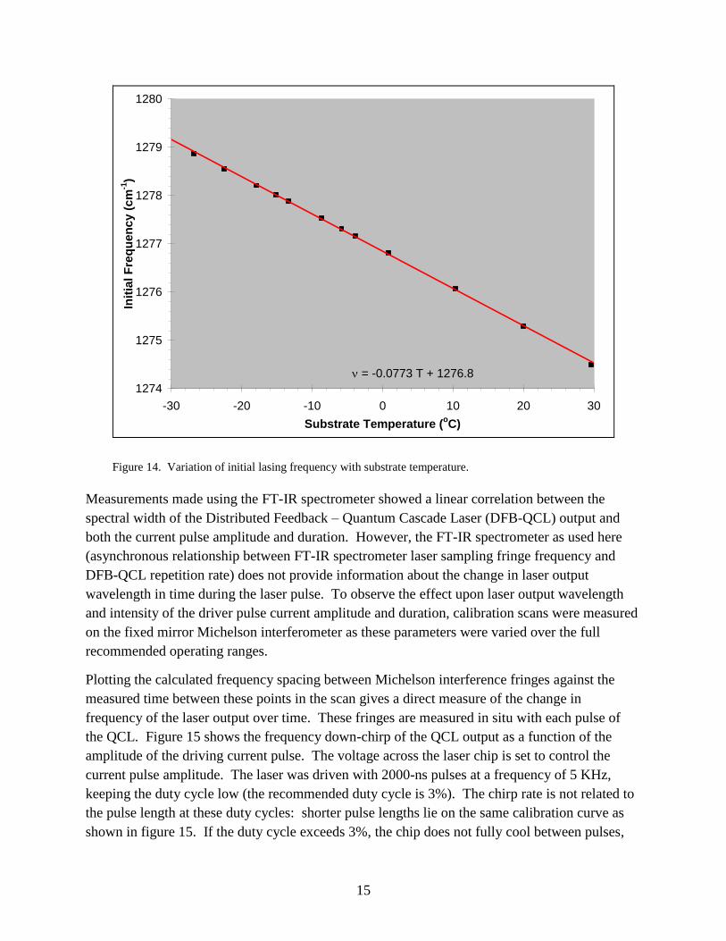
Figure 14. Variation of initial lasing frequency with substrate temperature. ...............................15
Figure 15. The frequency down-chirp of the QCL output as a function of the amplitude of the driving current pulse. .........................................................................................................16
Figure 16. Acetylene transmission spectra converted to spectral absorbance and plotted against a calibrated frequency scale. ........................................................................................17
Figure 17. Integrated absorbance plotted against acetylene concentration and partial pressure. ...................................................................................................................................19
Figure 18. The Bayer CFA............................................................................................................22
Figure 19. The color imaging processing pipeline. A generic outline of steps that must be taken to transform light collected by a lens to reproduce a full-color image suitable for viewing. ....................................................................................................................................22
Figure 20. A Bayer CFA pattern with a (3×3) kernel used to calculate the mean values of the RGB channels at pixel (3,3). ....................................................................................................23
Figure 21. White balance is performed to correct for the spectral distribution of the light source. The intensity has been normalized at 575 nm. ...........................................................24
Figure 22. The analytical calibration curve (blue curve) and measured data from a blackbody source (red triangles)................................................................................................................24

vi
Figure 23. A power law gamma correction relating the voltage from the sensor (Vin) and the voltage out or pixel value (Vout). ......................................................................................26
Figure 24. Spectral transmittance of the filters that comprise the CFA. .......................................27
Figure 25. Ratio of the green to red channel in the temperature range expected for detonation products. ...................................................................................................................................28
Figure 26. Surface temperature maps of exploding spheres of a nitramine-based high explosive. .................................................................................................................................31
Figure 27. Predicted velocity and temperature profiles for the opposed jet burner using Unicorn and Chemkin Pro, ethylene/air flame, Wang-Colket mechanism. .............................33
Figure 28. A comparison of calculated acetylene profiles in the opposed jet ethylene/air flame (calculations are also shown using the Wang-Frenklach mechanism [Wang and Frenklach, 1997]). ....................................................................................................................33
Figure 29. Photographs of the opposed jet ethylene/air flame with increasing amounts of metaxylene added to the fuel gas. ............................................................................................34
Figure 30. Peak values of fluorescence/light scattering vs. fraction of metaxylene in fuel gas based on several series of measurements in the opposed jet burner, measured prior to rebuild of vaporizer apparatus. ................................................................................................35
Figure 31. Flame simulations using UNICORN (Katta et al., 2006), that predict increases in C6H6 (benzene) but modest changes in OH, with addition of metaxylene to the fuel side of ethylene/air flames. ..............................................................................................................36
Figure 32. (a) An example of a raw trace of centerline fluorescence intensity vs. height above fuel duct for neat (0%) and 4% fuel side addition of metaxylene to ethylene/air diffusion flames after vaporizer rebuild. (b) OH fluorescence intensity (centerline) for 0%–5% addition of metaxylene to the fuel side of the atmospheric pressure ethylene/air opposed jet flame. ....................................................................................................................37
Figure 33. Change in PAH fluorescence/light scattering along the centerline of the burner for ethylene/air opposed flow flames, with metaxylene added to the fuel side after the atomizer was rebuilt. ................................................................................................................38
Figure 34. A reconstruction of the acetylene concentration (not temperature corrected) measured in absorption in an acetylene-air flame supported by a glass blower’s torch. Concentration values are in arbitrary units. .............................................................................39
Figure 35. Measured acetylene absorption through the flame region of an ethylene/air opposed flow flame to which acetylene is added on the fuel side. ..........................................40
Figure 36. A photograph of the ethylene-air candle-like diffusion flame supported on a glass blower’s torch. .........................................................................................................................41
Figure 37. Temperature maps using the imaging pyrometer technique for acetylene-air and ethylene-air diffusion flames. ..................................................................................................41
Figure 38. The wavelength-resolved emission from three ethylene air flames ranging from a candle-like diffusion flame to a coflowing diffusion flame to an opposed jet flame. .............42
Figure 39. The imaging pyrometer technique applied to an opposed jet ethylene/air flame. .......43
Figure 40. Neat ethylene/air-opposed flow flame results from McNesby et al. (2005b). ............44

vii
Figure 41. Modeling predictions conducted at 1 atm with Cantera. .............................................45
Figure 42. Modeling predictions conducted at 2.04 atm (30 psi) with Cantera............................45
Figure 43. Modeling predictions conducted at 5 atm with Cantera. .............................................46
Figure 44. The modified high-pressure strand burner enclosure used to house the elevated pressure-opposed jet burner. ....................................................................................................47
Figure 45. The elevated pressure burner assembly in co-flow mode on the test bed. One of the sapphire window ports has been removed. ........................................................................47
Figure 46. The elevated pressure burner assembly in co-flow mode on the test bed, with the sapphire window port removed. The fuel/air duct is visible within the chamber interior. .....48
Figure 47. The elevated pressure-opposed flow rig, showing the gated intensified camera (CCD) used to image planar LIF. ............................................................................................49
Figure 48. A side view of the elevated pressure-opposed flow rig on the test stand. The IR cutoff filter is shown in front of the sapphire window through which flame images are recorded for temperature measurement. ..................................................................................49
Figure 49. A view of the elevated pressure-opposed flow rig looking from behind the Vision Research Phantom 7 camera used to record flame images. .....................................................50
Figure 50. A view of the elevated pressure-opposed flow rig looking from the gas flow controllers. ...............................................................................................................................50
Figure 51. A view of the elevated pressure-opposed flow rig. The opposing fuel and air ducts are visible within the burner enclosure interior. .............................................................51
Figure 52. Raw images of elevated pressure-opposed flow flames at constant molar flow rate taken using a high-speed camera. It was necessary to adjust the camera exposure for each run to avoid saturating the camera chip. ..................................................................................52
Figure 53. Peak centerline temperatures (K) for elevated pressure ethylene/air flames at constant molar flow and at constant strain. Elevated pressure-opposed flow burner, ethylene/air flame. Temperatures are calculated using images in figures 51 and 52. ............53
Figure 54. Peak intensity per pixel per microsecond exposure along the burner centerline for the red pixel matrices (570–700 nm) from images of elevated pressure-opposed flow ethylene/air flames. ..................................................................................................................53
Figure 55. Raw images of elevated pressure-opposed flow flames at constant strain rate taken using a high-speed camera. It was necessary to adjust the camera exposure for each run to avoid saturating the camera chip. ..................................................................................54
Figure 56. (Top) Intensity ratio vs. temperature comparison of Wien’s approximation and an exact solution. (Bottom) Error vs. intensity ratio between Wien’s approximation and an exact solution. ..........................................................................................................................57
Figure 57. Wavelength of peak specific intensity vs. temperature. ..............................................59
Figure 58. Schematic of the three-color integrating pyrometer rig. .............................................60
Figure 59. Comparison of solar radiation both outside the atmosphere and at sea level with emission from an ideal blackbody at 5900 K. The baselines have been shifted for clarity. ...62

viii
Figure 60. (Top) Schematic of the single-axis two-color imaging pyrometer showing the lens and beam splitter arrangement. (Bottom) Band pass of each camera superimposed upon the emission from a blackbody near 2000 K. ..........................................................................63
Figure 61. (Top) Schematic of the full-color imaging pyrometer showing the Bayer-type mask in front of the sensor chip. (Bottom) Pixel calibration example from a Vision Research Phantom 5.1 camera. ................................................................................................65
Figure 62. (Top) Wavelength-resolved emission for three types of ethylene/air flames. (Bottom) Detail of emission from the OPPDIF flame showing emission bands due to CH and C2. ......................................................................................................................................66
Figure 63. Raw three-color integrating pyrometer data for a 227-g spherical C-4 charge, 19.0-cm standoff. .....................................................................................................................67
Figure 64. (Left) Calculated three-color integrating pyrometer temperatures for a 227-g spherical C-4 charge at 19.0-cm standoff. (Right) Average temperature profile from the three calculated temperatures. ..................................................................................................68
Figure 65. Average three-color integrating pyrometer calculated temperature profile for a 227-g spherical C-4 charge at 19.0-cm standoff. .....................................................................69
Figure 66. Average temperature profile calculated from all charges at a specified standoff distance with the three-color integrating pyrometer. ...............................................................70
Figure 67. Average three-color integrating pyrometer calculated temperature profile for the three 454-g spherical C-4 charges at 44.4-cm standoff distance, compared to the average temperature profile from the 227-g charges at that standoff....................................................71
Figure 68. Two-camera imaging pyrometer calculated temperature maps and corresponding histograms. Time sequence: a < b < c < d. The fireball reaches full size sometime between temperature maps a and b. .........................................................................................72
Figure 69. Calculated gas temperature at the steel table surface using the two-color imaging pyrometer for the charge shown in figure 68. ..........................................................................73
Figure 70. Full-color pyrometer extracted gas temperatures at the steel table surface vs. time for 227-g C-4 charges at the five standoff distances................................................................74
Figure 71. Gas temperatures at the steel table surface for the 227- and 454-g charges at a standoff of 44.4 cm. .................................................................................................................75
Figure 72. Average optically measured peak shock wave pressure at the steel table surface for the 227-g C-4 charges at the five standoff distances measured. ........................................76
Figure 73. Emission spectrum for the charge shown in figure 15 (227 g of C-4 at 63.5-cm standoff). The feature (doublet) near 589 nm is from sodium (Na) emission. .......................77
Figure 74. Temperatures measured for a 227-g C-4 charge at 63.5-cm standoff using each pyrometry method. ...................................................................................................................78

ix
List of Tables
Table 1. Temperature dependence of the line strength of the P(23) absorption line of the (υ4+ υ5) compound bending vibration of C2H2.........................................................................20

x
Preface
This report summarizes a 5-year effort at the U.S. Army Research Laboratory (ARL) to study
soot formation in diffusion flames. The work described in what follows begins with
experimental and modeling studies of atmospheric pressure ethylene (C2H4)/air (N2-O2) flames
to which metaxylene (C8H10) is added on the fuel side. Several laser-based diagnostic methods
are discussed, including an extensive effort to measure acetylene gas in flames using a quantum
cascade laser. The report also describes efforts to construct an elevated pressure-opposed flow
burner and presents data on soot formation in ethylene/air flames in this burner to a total pressure
of ~3 bar. During the course of this work, new experimental techniques of high-speed digital
temperature and pressure mapping were developed. These techniques, described here in detail,
became the focus of the latter part of the research. They are also applied to flame analysis and
explosion measurement as a way of illustrating the ability to measure pressure and temperature
during dynamic events. The report finishes with a discussion of unresolved or incomplete
questions and tasks, and a list of publications.
Overall, ARL’s effort on this overall task was moderately successful. The elevated pressure-
opposed flow burner required 3 years to become operational (this includes an 8-month safety
stand down at the laboratory). Several planned experiments at elevated pressure have yet to be
completed. A major accomplishment of this study is the establishment at ARL of a working
elevated pressure-opposed flow burner equipped for analysis using active laser-based methods.
The development of several new high-speed pyrometry measurements during this program
should prove valuable in the long term to the combustion and explosion community. We believe
this aspect of the work will advance the application of digital imaging to measurement of
physical parameters of flames and explosions.

xi
Acknowledgments
The authors wish to thank Dr. Mel Roquemore and Prof. Tom Litzinger for the helpful, honest
assessments of this work, and Dr. Eric Bukowski for a detailed review of this manuscript.
The authors would also like to thank the Strategic Environmental Research and Development
Program for funding the developmental work on the elevated pressure burner, the quantum
cascade laser for acetylene measurement, and the two-color and full-color pyrometer rigs. The
Department of Homeland Security provided support for some of the exterior testing. Support is
also acknowledged from the Defense Threat Reduction Agency. This research was supported in
part by an appointment to the U.S. Army Research Laboratory (ARL) Postdoctoral Fellowship
Program administered by the Oak Ridge Associated Universities and National Research Council
through a contract with ARL. Support was also provided by a grant from the National Research
Council.

xii
INTENTIONALLY LEFT BLANK.

1
1. Testing Rigs
1.1 Opposed Jet Diffusion Flame
1.1.1 Introduction
Previous Strategic Environmental Research and Development Program (SERDP)-related studies
using the U.S. Army Research Laboratory (ARL) opposed jet diffusion flame burner have
concentrated on soot formation in atmospheric pressure ethylene/air flames (McNesby et al.,
2005b). For the current program investigating soot formation, this burner has been modified to
operate at fuel side temperatures up to 250° centigrade, enabling the use of many fuels that are
liquids at room temperature. Opposed jet diffusion ethylene/air flames have also been
investigated at elevated pressure (5-bar total pressure) using an opposed jet burner flame
apparatus constructed at ARL. The flames supported in these burners are probed using several
types of optical diagnostics, including laser-induced fluorescence (LIF), laser scattering, tunable
diode laser absorption spectroscopy (TDLAS), and multicolor pyrometry. The experimental
apparati, methods, and techniques developed for the ARL effort are described in what follows.
1.1.2 Opposed Jet Diffusion Flame Experimental Setup: Background
An opposed jet burner consists of opposing, parallel gas ducts separated by a distance near to the
duct diameter. Typically, the ducts are arranged vertically, with fuel gases flowing upward from
the lower duct and oxidizer gases flowing downward from the upper duct. After the gases exit
the ducts, they travel a short distance in free space before colliding with each other. For gases of
approximately equal densities, a stagnation plane occurs midway between the ducts where the
axial velocities of the colliding gas streams approach zero. For the sooting opposed flow flames
used in this program, peak soot concentration typically occurs near the stagnation plane, in fuel-
rich regions at temperatures slightly lower than peak combustion temperatures (Hwang and
Chung, 2001). The gas flows, duct arrangements, and stagnation plane are conceptually shown
in figure 1. For these experiments, the stagnation plane location may be estimated by calculation
and visualized using fluorescence techniques.
For opposed flow diffusion flames in which the stagnation plane is fuel rich (e.g., the flames
reported here), the flame occurs at the location where fuel and oxidizer are close to
stoichiometric combustion proportions. This occurs on the oxidizer side of the stagnation plane
(see figure 1), and the stoichiometric mixture is achieved by fuel gases diffusing upstream into
the oxidizer flow. For the ethylene/air flames, the overall chemical reaction (assuming air to be
20% oxygen) is
C2H4 + 3O2 + 12 N2 2CO2 + 2H2O + 12 N2 . (R1)

2
Figure 1. A schematic of the opposed flow burner showing
gas flow and flame location.
Reaction R1 shows that for fuel (C2H4) and oxidizer (air) flow rates that are approximately equal,
in an opposed flow burner (our conditions), assuming gases with similar momenta (our
conditions), the gas mixture at the stagnation plane will be fuel rich (Hwang and Chung, 2001).
Because of this, regions of highest particulate and aromatic concentrations (sooting region) and
the main combustion (flame radical production) region in opposed flow flames are physically
separated (Hall et al., 1997). A photograph of an ethylene/air-opposed jet flame, at atmospheric
pressure, showing the separation of sooting and combustion regions, is shown in figure 2.
1.1.3 Burner Configuration: Atmospheric Pressure
The opposed flow burner is constructed of 304 stainless steel and is based upon the design of
Lentati and Chelliah (1998). Fuel gas and oxidizer (air) ducts are 15 mm in diameter and are
separated by 7 mm. A photograph of an ethylene/air flame within the burner chamber is shown
in figure 3. Flow rates for the experiments reported here are typically 4.6 L/min fuel and 6.2
L/min air. These values were chosen because they gave the most stable flame. When fuels are
used that are liquids at room temperature, they are injected into heated fuel lines (see description
in next section) using an injection pump (Isco). A shroud gas (nitrogen) surrounded both fuel
and oxidizer ducts within the burner assembly to minimize entrainment of room air into the
flame. The burner was enclosed in a chamber that was capable of being evacuated. However,
for the atmospheric pressure experiments, the access ports of the chamber were left open. A
schematic of the experimental apparatus, including some optical diagnostics, is shown in figure 4.
Air Duct
Fuel Duct
Luminous Flame
Region
Sooting Region
Atmospheric pressure
C2H4/air flame – N2 shroud
Stagnation Plane 1 cm

3
Figure 2. A photograph of an ethylene/air-opposed jet flame showing
the separation of sooting and combustion regions.
Figure 3. A photograph of an ethylene/air flame within the burner chamber.

4
Figure 4. A schematic of the experimental apparatus, including some optical diagnostics.
1.1.4 Burner Configuration: Elevated Pressure
The elevated pressure-opposed flow burner is constructed of 304 stainless steel and, similar to
the atmospheric pressure burner, is based upon the design of Lentati and Chelliah (1998). Fuel
gas and oxidizer (air) ducts are 15 mm in diameter and are separated by 6 mm. This distance
was used because it gave a stable flame. Originally, a separation distance of 7 mm was called for
in design. However, pressure sealing problems after construction called for a slight design
modification, which decreased the duct separation by 1 mm. For the elevated pressure burner,
the fuel and oxidizer ducts and flame shroud ducting are contained within an enclosure of 304
stainless steel initially designed for a strand burner The enclosure is rated to withstand pressures
to 130 bar (~2000 psi). The high-pressure enclosure is equipped with two sapphire windows
(25-mm diameter) for emission and transmission of probe radiation, and two PMMA
(polymethyl methacrylate) windows (25 × 100 mm) for flame observation. Using a high-volume
enclosure, we had problems in previous efforts with unburned fuel and air exploding and
damaging windows. The current design minimizes chamber interior volume. A photograph of
the elevated pressure burner with one sapphire window port removed is shown in figure 5. At
the time of this report, the flow rates giving most stable flames at elevated pressure were ~5 L/min
ethylene and 4 L/min air. A shroud gas (nitrogen) surrounded both fuel and oxidizer ducts
within the burner assembly to minimize flame formation away from the vicinity of the fuel and
oxidizer ducts. It was necessary to bathe all windows in a nitrogen shroud to prevent
condensation. A schematic of the elevated pressure experimental apparatus, including some
optical diagnostics, is shown in figure 6.
XeCl Excimer Laser Dye Laser DoublingCrystal
Oxidizer
Fuel
ICCD Camera
PressureChamber
CylindricalLens
Flame
PC
TurningPrismIris

5
Figure 5. Photo of elevated pressure rig in opposed flow configuration.
Figure 6. Schematic of elevated pressure rig.
Oxidizer
Fuel
Flame
N2 in (window shroud) N2 in (window shroud)
N2 in (pressure adjustment)
Vacuum out (pressure adjustment)
High speed digital video

6
1.1.5 Fuel Introduction: Atmospheric Pressure Burner
The liquid fuel vaporizer consists of a Collison-type atomizer that uses a preheated nitrogen gas
stream as a carrier (figure 7). Fuel is introduced into the atomizer by an Isco syringe pump.
Figure 8 shows a diagram of the vaporizer apparatus integrated into the burner system. The
Collison-type atomizer is immersed in an Al2O3 fluidized bath (Techne, Inc., model SBS-4).
Additionally, the fluidized bath is used to preheat all feed gases to the atomizer. Transfer lines
from the fluidized bath to the burner are heated using thermostatically controlled heating tape
(Omega). Figure 9 shows a photograph of the burner assembly, the syringe pump, and the
fluidized bath.
Figure 7. The Collison-type atomizer.
Preheated, 200C,
60 psi
Exit gas temp to200C
Exit gas pressure 1 atm
Fuel in
from Isco pump
(260ml cap.)

7
Figure 8. A diagram of the vaporizer apparatus integrated into the burner system.
Figure 9. A photograph of the burner assembly, the syringe pump, and the fluidized bath.
burner
preheat
Injection pump
Mass flow

8
1.1.6 Fuel and Oxidizer Introduction: Elevated Pressure Burner
For the elevated pressure burner, all gasses were used at ambient pressure. The main difference
between fuel introduction for the elevated pressure rig and the atmospheric pressure rig was an
increase in back pressure for the flow controllers. In general, gas flow controller back pressure
was maintained ~20 psi (1.25 bar) above burner chamber pressure.
1.1.7 Experimental Procedure: Atmospheric Pressure Flames
For atmospheric pressure-opposed jet flames using a vaporized liquid as a fuel component, the
experimental procedure was as follows. The gas flow controllers (MKS Corp.) were turned on
and allowed to warm up for ~1 h. The nitrogen flow to the underside of the fluidized bed was
initiated, and the fluidized bed heaters were turned on. Heaters and temperature controllers for
all gas transfer lines and burner heaters were turned on. The fuel carrier gas to the Collison
atomizer (nitrogen) was turned on, and the back pressure to the atomizer adjusted to ~15 psi.
Shroud gas flow to the burner was turned on. The rig was allowed to warm to operating
temperature (e.g., for fuel additive metaxylene, bath and lines were set to 200° centigrade).
When the operating temperature was reached, a flame source was placed between the burner
ducts and ethylene gas, and airflow was commenced, with the opposed flow flame igniting
immediately. The nitrogen shroud gas flow (5 L/min total) was initiated, and the flame was
allowed to stabilize for 5 min. For experiments using fuel additive, a valve on the injection
pump was opened, and flow of liquid fuel into the Collison atomizer was begun. After ~1 min of
flow of liquid fuel and a visual inspection of the flame to check for pulsation (an indication of
incomplete vaporization), measurements were begun.
1.1.8 Experimental Procedure: Elevated Pressure Flames
For elevated pressure opposed jet flames, gas flow controllers (MKS) were turned on and
allowed to warm up for ~1 h. Fuel (ethylene), oxidizer (air), and shroud gas (nitrogen) back
pressures were adjusted to ~4 bar (60 psi). Prior to flowing any gas, a flame was placed between
the burner ducts and ethylene gas, and airflow was commenced, with the opposed flow flame
igniting immediately. The nitrogen shroud gas flow (5 L/min total) was initiated, and the flame
was allowed to stabilize. Suction from the pump used to evacuate the system (Leybold,
Fomblin-charged) was minimized, and the burner chamber sealed by screwing in the window
port removed to allow lighting. The flame was allowed to stabilize at slightly less than
atmospheric pressure (typically 0.75 bar [570 torr], and nitrogen flow via the window shroud was
initiated. To increase pressure up to ~1.75 bar (11-psi gauge), nitrogen gas was added through
the window shroud port while keeping gas evacuation rate constant. Above 1.75 bar, a
combination of increased nitrogen flow and further restriction of exhaust gas pumping was used.

9
1.2 Explosives Test Bay
Experiments were conducted at an outdoor test range at Aberdeen Proving Ground (APG). The
test range consisted of a rectangular concrete deck, ~2100 m2, surrounded by barricaded control
buildings. The experimental apparatus consisted of an explosives test rig and optical diagnostics
test rig separated at the center of the concrete deck by ~12 m. The explosives test rig was
centered on a 1.5m2 table positioned 0.84 m above the concrete deck. The table surface was an
8.26-cm-thick steel plate. Explosive charges were suspended over the table center by nylon
string at standoff distances of 12.7, 19.0, 31.8, 44.4, and 63.5 cm. Detonation was initiated by an
RP-83 exploding bridge-wire detonator. Diagnostic instrumentation was triggered by rupturing
an illuminated 600-μm Si core optical fiber placed adjacent to the charge apex. Upon explosive
initiation, a trigger pulse was generated because of the abrupt loss of light transmission through
the fiber.
The multi-imaging rig consists of four separate instruments: a three-color integrating pyrometer,
a two-camera imaging pyrometer, a full-color single-camera pyrometer (Densmore et al., 2011),
and a wavelength-resolved spectrograph (300–800 nm). Each pyrometer in the imaging rig
operates on the same scientific principle: determining temperature from spectral emission
intensity. The rig was enclosed in 1- × 1- × 2-m-tall armored enclosure (2.54-cm-thick steel)
with an ~30 cm2 viewing port positioned 1.22 m off the concrete deck. The viewing port was
uncovered to prevent the need to calibrate the pyrometers through window material and also
because there was no anticipated fragment danger from the uncased C-4 charges. A diagram of
the full test rig setup is shown in figure 10.
Figure 10. The explosives test bed and assorted instrumentation composing the multipyrometry rig.
3-color integrating
pyrometer
2-color imaging
pyrometer
Full color imaging
pyrometer
Integrating
spectrograph
25 inches
0.5 pound C-4
Steel
table
Concrete deck
10 m
Apertured,
armored enclosure
3-color integrating
pyrometer
2-color imaging
pyrometer
Full color imaging
pyrometer
Integrating
spectrograph
25 inches
0.5 pound C-4
Steel
table
Concrete deck
10 m
Apertured,
armored enclosure

10
2. Diagnostic Methods
2.1 Laser Fluorescence/Scattering
The experimental method has been discussed in detail previously (McNesby et al., 2005b). A
sheet of pulsed laser radiation (typically 0.5 mJ/pulse, ~20-ns duration, formed using a double-
apertured, half-cylindrical lens) near a wavelength of 281 nm was passed through the flame
region. A gated, unfiltered, intensified charge-coupled device (CCD) camera (Roper Scientific,
256 × 1024 pixels) equipped with a Nikor 1:4.5 UV lens was used to measure laser scatter during
and immediately following the laser pulse (camera gate width = 80 ns). The images produced by
100 laser pulses were averaged in the camera memory. An image obtained in this way for an
ethylene/metaxylene (5%)/air flame is shown in figure 11. From this average image, the
maximum value at a given pixel location along the centerline between the fuel and oxygen ducts
was selected in the sooting and combustion regions of the flame. A background value at that
pixel location, measured prior to the flame initiation (also 100 averaged images), was subtracted
from this value. This background corrected pixel value became the data point representing peak
particle or OH concentration.
Figure 11. A Planar Laser-Induced Fluorescence image of an ethylene/metaxylene (5%)/air-opposed jet flame.
Lambda Physik Excimer/Scanmate system: Coumarin 153 dye: fundamental at 560 nm, 2× frequency to 281 nm; pump
A2Σ+ (v = 1) ←X2Π (v = 0), detect (0,0), (1,1) around 310 nm.

11
Following data collection, the injection pump valve was closed, the pump flow parameters were
reset, and the process repeated. Planar LIF and light scatter measurements at the beginning and
end of each run series were performed to check that the flame returned to normal after the
ethanol flow was stopped. Laser power was measured before and after each experimental run
and typically varied by <2%. Other than subtraction of background, no corrections were made
for changes in laser power or variations in spatial intensity, and no other specific dark field pixel
corrections were made, although previous measurements of the CCD dark field (camera blocked)
showed pixel-to-pixel output to vary by <2%. A schematic of this setup is shown in figure 4.
2.2 Tunable Diode Laser Absorption Spectroscopy
Tunable diode laser spectroscopy was chosen to quantify acetylene formation in the opposed jet
diffusion flames. Measuring the acetylene produced in the flame provides a metric for
monitoring the soot production. Quantifying trace gas species concentration within a flame by
laser absorption is a nontrivial measurement. The instrument must be sensitive and selective to
distinguish weak signals from the target molecule from the myriad of other species produced in a
combustion reaction. The inherent difficulty of measuring absorption spectra at high
temperature—where the population of initial states is spread over a much greater number of
accessible states—is made even more difficult by measuring through turbulent flows of mixed
gasses in excited states. To perform this measurement, we have built and characterized a
sensitive, selective infrared (IR) absorption spectrometer system capable of measuring, in real
time, absolute acetylene concentration in low concentration samples at elevated temperature.
This system is designed around a pulsed distributed feedback Quantum Cascade Laser (QCL).
Recent work shows the QCL to be an extremely useful tool for TDLAS (Kosterev and Tittel,
2002). The QCL operates near room temperature and provides a powerful (~10 mW), stable,
single-mode, mid-IR light source suitable for tunable laser spectroscopy. Nearly the entire IR
spectrum is accessible to quantum cascade lasers, as the laser emission is determined by the
growth of the substrate interstitial layer spacing—not the composition—and a wide spectral
range is accessible to a single QCL by temperature tuning the substrate. The QCL used in this
experiment is designed for pulsed, single longitudinal mode emission over a thermally tunable
range of 1279 to 1273 cm–1
.
A frequency down-chirp is inflicted on the output of the pulsed diode laser as a result of resistive
heating as the current pulse deposits energy into the diode chip. There are two methods for
working with this frequency chirp: inter- and intra-pulse spectroscopy. Inter-pulse spectroscopy
minimizes the effect of the chirp by driving the QCL with ultra-short pulses (3–5 ns), resulting in
near-Fourier-limited laser pulses that are scanned through the spectral range of interest by
temperature tuning (Harris and Weiner, 1983) or a subthreshold ramp (Kosterev and Tittel,
2002). Typical resolution of δν < 0.01 cm–1
is attainable by this technique.

12
Intra-pulse spectroscopy harnesses the near linearity of the frequency down-chirp to scan through
a spectral region in a single long laser pulse (100 ns – several microseconds). The resolution of
this technique is limited by the scan rate: δν = (C*dν/dt)½, where C is a form factor dependent on
the pulse shape—for long square pulses, C = 0.883 (Normand et al., 2001). Both techniques
yield similar resolution. Inter-pulse spectroscopy can scan much longer spectral ranges (up to
30 cm–1
has been reported [Kosterev and Tittel, 2002]) but requires complex computer control of
the driving current supply and long timescales for signal collection as the laser is scanned
through the spectral range. The intra-pulse technique is characteristically simple, yielding
spectra similar to a cropped selection of a broadband absorption spectrum; however, the
maximum spectral range is limited to a few wave numbers.
The real-time response of the intra-pulse technique makes it attractive to studies of flame species
concentration. The turbulent gas flow, steeply varying temperature/density of the flowing
gasses, and onset of scattering soot particles all give rise to significant random fluctuations in the
transmitted intensity. These variations yield line distortions and false peaks in the ratioed
absorption spectrum if the time for scanning a spectral line is comparable to these environmental
variations. Subthreshold current tuning has millisecond scan times, and temperature tuning of
the substrate responds on the order of 1 min; the microsecond response time of the QCL allows it
to analyze a frozen flame. The typical maximum spectral range attainable in the intra-pulse
tuning method is just over 2 cm–1
. This is only broad enough to scan a single acetylene
absorption line because of the large rotational constant of acetylene, but even when the peak is
broadened by high pressures, the range is large enough to scan beyond the range and collect a
background with each scan. To our knowledge, this is the first measurement of absorption
spectroscopy within flame made with this chirp-based QCL technique.
The distributed feedback QCL used in this experiment (developed at Alpes Laser, Switzerland,
supplied by Boston Electronics) is designed for pulsed, single longitudinal mode emission at
7.86 µm. The QCL substrate temperature and the driving pulse (current amplitude, pulse length,
and frequency) are controlled via laptop running LabView control VI (Cascade Technologies).
The QCL is mounted on a Peltier thermoelectric cooler, which can vary the substrate temperature
from –30 to 30 °C stabilized to 0.01 °C. The output is collimated through ZnSe optics housed
inside the sealed laser head and exits the case in a roughly collimated beam with waist ~1 mm.
A schematic of the experimental setup is presented in figure 12. For flame measurements, the
laser beam is sent directly through a single pass 16-cm path length gas absorption cell with
wedged BaF2 windows and then through the flame. The gas cell is used to check absorption line
position and is evacuated for quantitative flame measurements. The transmitted light is
measured by a fast-rising, Peltier-cooled (HgCdZn)Te detector (VIGO PVI-2TE-10) and
recorded using a high-speed signal averager from Boston Electronics. The detectivity of the
photodetector is D* = 2 × 10⁹ cmHz
½/W and the rise time is under 0.3 ns.

13
Figure 12. A schematic of the experimental setup for acetylene measurement by QCL.
To characterize the laser output wavelength, the beam is sent through a fixed-mirror Michelson
interferometer, built to dynamically measure the change in frequency of the laser output over the
course of the pulse. The light exiting the interferometer is measured on the same (HgCdZn)Te
detector. The wavelength range (∆ν, expressed in wave numbers, cm–1
) between two maxima
measured by the interferometer is a constant function of the geometry of the light path: ∆ν =
(2∆L)–1
, where ∆L is the path length difference between the two legs of the interferometer.
A typical example of laser output vs. time measured through the interferometer and the
evacuated gas absorption cell is shown in figure 13. Also shown in this figure is the time-
varying current pulse used to drive the laser. The sharp onset and constant amplitude of the
“top-hat” current pulse leads to abrupt lasing and nearly linear frequency down-chirp. There are
small reflections at the beginning of the pulse due to imperfect impedance matching in the cables
delivering the driving signal to the laser head; these reflections are not atypical of this type of
QCL system (Müller et al., 1999). The smaller modulation on the laser transmission is an
interference effect caused by multiple reflections within the beam splitter. This does not affect
the absorption measurements, as it is a consistent feature of the background when it is observed.
In figure 13, the fringe spacing of the Michelson interferometer is 0.1018(5) cm–1
and the total
usable spectral range of the pulse is about 2.2 cm–1
.

14
Figure 13. A typical example of laser output vs. time measured through the interferometer and the
evacuated gas absorption cell. Also shown is the time-varying current pulse used to drive the
laser.
2.2.1 Characterizing Tunable Diode Laser Output
To exploit the frequency down-chirp of the QCL, it is necessary to fully characterize the
temporal and spectral evolution of the laser output. The output of this QCL is set by four
controllable parameters: the bulk laser substrate temperature, the driving current pulse amplitude,
the driving pulse time duration, and the driving pulse repetition rate. Each affect the chirp rate
by controlling the heat dumped into the diode chip.
A high-resolution Fourier transform infrared (FT-IR) spectrometer (ABB-Bomem, model DA-8)
set to emission mode was used to calibrate the laser output wavelength as a function of substrate
temperature (temperature tuning). Measurements were made at the highest resolution and
slowest scanning rate of the Bomem FT-IR spectrometer to ensure the instrument viewed a
quasi-continuous light source from the pulsed QCL. The maximum resolution of this instrument
is 0.04 cm–1
, and the slowest scan speed is 0.05 cm/s. The bulk temperature of the Peltier-cooled
QCL was varied over the full suggested range, from –30 to 30 °C. Over this temperature range,
the initial lasing frequency of the QCL varied nearly linearly over 4.4 wave numbers (figure 14).
-5
0
5
10
15
20
-100 400 900 1400 1900
Time from Trigger (ns)
La
se
r In
ten
sit
y (
arb
. u
nit
s)
-0.5
0
0.5
1
1.5
2
Dri
vin
g C
urr
en
t (A
mp
s)
Michelson Transmission
Laser Intensity
Interference Fringes
Current Pulse
15
Figure 14. Variation of initial lasing frequency with substrate temperature.
Measurements made using the FT-IR spectrometer showed a linear correlation between the
spectral width of the Distributed Feedback – Quantum Cascade Laser (DFB-QCL) output and
both the current pulse amplitude and duration. However, the FT-IR spectrometer as used here
(asynchronous relationship between FT-IR spectrometer laser sampling fringe frequency and
DFB-QCL repetition rate) does not provide information about the change in laser output
wavelength in time during the laser pulse. To observe the effect upon laser output wavelength
and intensity of the driver pulse current amplitude and duration, calibration scans were measured
on the fixed mirror Michelson interferometer as these parameters were varied over the full
recommended operating ranges.
Plotting the calculated frequency spacing between Michelson interference fringes against the
measured time between these points in the scan gives a direct measure of the change in
frequency of the laser output over time. These fringes are measured in situ with each pulse of
the QCL. Figure 15 shows the frequency down-chirp of the QCL output as a function of the
amplitude of the driving current pulse. The voltage across the laser chip is set to control the
current pulse amplitude. The laser was driven with 2000-ns pulses at a frequency of 5 KHz,
keeping the duty cycle low (the recommended duty cycle is 3%). The chirp rate is not related to
the pulse length at these duty cycles: shorter pulse lengths lie on the same calibration curve as
shown in figure 15. If the duty cycle exceeds 3%, the chip does not fully cool between pulses,
n = -0.0773 T + 1276.8
1274
1275
1276
1277
1278
1279
1280
-30 -20 -10 0 10 20 30
Substrate Temperature (oC)
Init
ial
Fre
qu
en
cy
(c
m-1
)

16
Figure 15. The frequency down-chirp of the QCL output as a function of the amplitude of the driving
current pulse.
and increasing the pulse length or pulse frequency will affect the chirp rate. The damage
threshold for the laser quoted by the supplier was I ≥ 4.0 A. With the driving current amplitude
of 3.48 A, the thermoelectric cooler could not keep the substrate temperature at the set point and
the laser output drifted in frequency over the course of minutes. To avoid damaging the chip,
our data was taken at lower current amplitudes of 1.80 A, which provided smooth, reproducible
chirp behavior and no measured long-term drift. As is evident in figure 15, for pulses <400 ns
the chirp rate is essentially constant, and the frequency is linearly related to the scan time;
however, for longer pulses, the nonlinear response of the lasing material must be taken into
account for proper calibration.
2.2.2 Acetylene Absorption in Gas Cell
Absorption spectra of acetylene vapor in a single pass absorption cell were measured to test the
accuracy and sensitivity of the spectrometer by comparing the measured absorption against the
well-characterized standard for the acetylene cross section, as reported in the HITRAN (high-
resolution transmission) database (Jacquemart et al., 2003).
nREL = 2.445E-13t4 - 1.279E-09t
3 + 2.633E-06t
2 - 3.391E-03t + 1.861E-01
-6
-5
-4
-3
-2
-1
0
0 500 1000 1500 2000
Pulse Time (ns)
Fre
qu
en
cy
Do
wn
-Ch
irp
(c
m-1
)
1.28A
1.46A
1.48A
1.80A
2.09A
2.57A
3.11A
3.48A
1.46 A
1.48 A
1.28 A
1.80 A
2.09 A
2.57 A
3.11 A
3.48 A

17
The absorption band of the (υ4+ υ5) compound bending vibration of acetylene is centered near
1330 cm–1
, the rotational constant of acetylene is 1.125 cm–1
. The higher J-value transitions of
the P-band are relatively unobscured by absorption from atmospheric gases (e.g., H2O, CO2,
etc.). The P(23) rotational line at 1275.512 cm–1
is measured in this experiment as it is near the
peak of the P-branch at the elevated temperatures that is encountered when probing flames. The
transmitted laser intensity is recorded on the photodiode through varying partial pressures of
acetylene gas diluted to one atmosphere total pressure in lab air. These room temperature
transmission spectra are converted to spectral absorbance and plotted against a calibrated
frequency scale in figure 16. The central absorption feature in these spectra is the P(23)
absorption line of the (υ4+ υ5) compound bending vibration of C2H2; the smaller features in the
spectrum are currently unidentified.
Figure 16. Acetylene transmission spectra converted to spectral absorbance and plotted against a calibrated
frequency scale.
These absorbance spectra are analyzed in SigmaPlot to extract the line strength from the data.
The spectra are taken in the Beer-Lambert approximation, where the absorbance is linearly
related to the concentration of absorbers [X] and optical path length L by the absorption cross
section σ (ν):
0
0.2
0.4
0.6
0.8
1
1.2
1.4
1275 1275.5 1276 1276.5 1277
Frequency (cm-1
)
Ab
so
rban
ce
0.95 Torr
2.5 Torr
3.1 Torr
4.2 Torr
8.2 Torr
19.2 Torr

18
LXgSLXI
IA
o
][)(][)(
)(
)(ln)( nn
n
nn . (1)
In the final relation, S* g(ν) is the line strength of the absorption feature multiplied by a
normalized peak function. The absorbance spectra are fit to the multi-Lorentzian function
(equation 2):
i oii
ii
i
i
AfF
nn
nn
2)()( , (2)
where ν is the frequency in cm–1
, the sum runs over five peaks centered at ν oi, and γi is the
species-specific peak width. There is no constant background offset as the absorption features
fall to zero by the end of the laser pulse scan. The integrated absorbance of each peak, Ai ,
contains the line strength (cm–1
/(molecules cm–2
)), the concentration (molecules*cm–2
), and the
absorption length (cm):
LXSdfA HCHCHC ][222222 nn . (3)
The normalized Lorentzian peak function is chosen over the Voigt peak conventionally used in
laser absorption spectroscopy because both return equivalent fits to the pressure broadened
absorbance peaks, and there is evidence that the Voigt profile is not theoretically appropriate in
fast frequency-chirped spectra (Duxbury et al., 2007).
Plotting the integrated absorbance in equation 3 against the product of the optical length and the
acetylene concentration (converted from the partial pressure of gas in the cell) gives a measure of
the line strength parameter that can be compared to the value listed in HITRAN, S = 2.218 ×
10–20
cm–1
/(molecules cm–2
). The integrated absorbance is plotted against acetylene
concentration and pressure in figure 17, showing a linear relationship in fairly good agreement
with the predicted absorbance. The scatter about the predicted line is larger than explained by
the quality of the fit or the standard deviation of repeated measurements of a sample. The most
likely cause of this scatter is imprecise measuring of sample pressure, yielding incorrect
predicted concentrations. The gas delivery system that was used to fill the absorption cell had
leaks that could not be fully sealed in the course of the experiment, and assigned pressures of the
samples could be off by as much as 10%. A linear, least-squares fit of the data, using the path
length 16 cm, gives a line strength S = 2.36 (±0.18) × 10–20
cm–1
/(molecules cm–2
), in agreement
with the accepted value. With the signal-to-noise level measured in the individual spectral scans,
based on the root-mean-square noise in the baseline of the spectrum, we can accurately measure
absorption features with peak heights of 1.5 × 10⁻⁴
absorbance units, corresponding to an
acetylene concentration*length product of 2.4 ppM-m (parts per million meter).

19
Figure 17. Integrated absorbance plotted against acetylene concentration and partial pressure.
The line strength is dependent on the population difference between the two levels of the
specified transition, and as the temperature increases, so does the number of accessible initial
states according to classical Boltzmann statistics. The population difference between the initial
and final states in a transition at a temperature T is
kT
hcv
kT
hcE
TQ
NNN iiTotal exp1
"exp
)(''' , (4)
where E” is the initial state energy and νi = E’-E” is the energy of the transition, Q(T) is the
temperature-dependent partition function. Therefore, the temperature dependence of the
absorption line strength is the ratio of the line strength at the measured temperature and some
reference temperature (all HITRAN parameters are all listed at a reference temperature
Tref = 296 K).
ref
i
i
ref
i
refrefi
i
kT
hc
kT
hc
TTk
hcE
TQ
TQ
TS
TS
n
n
exp1
exp111"
exp)(
)(
)(
)(. (5)
0
0.02
0.04
0.06
0.08
0.1
0.12
0.14
0 2 4 6 8 10 12 14 16
Acetylene Concentration (ppt)
Inte
gra
ted
A
bs
orb
an
ce
(c
m-1
)0 2 4 6 8 10 12
Acetylene Partial Pressure (Torr)
Hitran PredictionMeasured Absorbance

20
For the P(23) absorption line measured in this work, the line strength peaks at T = 500 K. As
shown in table 1, the line strength initially increases as temperature begins to rise and the band
center shifts to higher J values, but at the peak flame temperature of an acetylene/air flame,
T ~ 3000 K, the line has fallen to <0.3% of its initial strength.
Table 1. Temperature dependence of the line
strengtha of the P(23) absorption line of
the (υ4+ υ5) compound bending vibration
of C2H2.
Temperature
(K)
Line Strength(/10–20
)
(cm–1
/molecule cm–2
)
296 2.2180
400 2.9598
470 2.9624
600 2.4464
800 1.4687
1000 0.81326
2000 0.049290
3000 0.0069049
aAs predicted in the HITRAN database.
2.3 High-Speed Digital Optical Pyrometry
2.3.1 Introduction
Temperature measurements of fast, destructive events (e.g., combustion or high-explosive
detonations) present many challenges. Conventional methods employing thermocouples,
resistance temperature detectors, or diodes are intrusive and suffer from slow response times.
Optical pyrometry is an alternative method that offers advantages over these conventional
methods. Optical pyrometers are capable of operating at large standoff distances from the
experiment, negating the potential for damage, and possess response times in the gigahertz range.
High-speed optical pyrometry possessing high spatial and temporal resolution may be achieved
with digital color imaging devices that use either CCDs or complementary metal oxide
semiconductor (CMOS) sensors. IR focal plane arrays with InSb photodiodes have been used to
measure temperatures of in-flight slugs fired from rifles (Richards, 2005). Visible spectrum
optical pyrometers using CCD or CMOS sensors have been developed by a number of groups.
T. Fu and coworkers have performed extensive work on the theory and optimization of color
imaging pyrometers (Fu et al., 2004; Fu et al., 2006a; Fu et al., 2006b; Fu et al., 2008).
Pyrometers based on either CCD or CMOS color imaging devices have been used to measure
soot temperature and concentrations (Fu et al., 2010; Lu et al., 2009; Simonini et al., 2001), laser
weld temperatures (Bardin et al., 2004), and silicone carbide fibers (Maun et al., 2007).

21
We have characterized and calibrated a high-speed Phantom Vision Research (Vision Research,
2010) color camera for use as an optical pyrometer. Complete calibration of the digital color
camera is required for its use as a pyrometer. The two components that need to be characterized
are the color filter array (CFA) sensitivity and an overall calibration factor. Raw grayscale data
from the CFA are used in conjunction with a physical model to determine the temperature of the
imaged scene. The fundamental basis for the analysis assumes that the collected light is from a
self-luminous object that behaves as a graybody emitter. The analysis follows the two-
wavelength ratio method (DeWitt and Nutter, 1988; Grum and Becherer, 1979), extended to the
broadband regime, using the light intensity collected from the CFA. Temperature calculations
can be performed on movie or image files if the color-imaging pipeline is taken into account.
The color image–processing pipeline performs operations on the raw CFA data that could
potentially introduce errors in the apparent temperature. Processing operations that may corrupt
the data and cause an erroneous temperature are discussed in section 2.3.2.
2.3.2 Digital Color Imaging
Most high-speed color cameras consist of a panchromatic complementary metal-oxide-
semiconductor imaging sensor that is sensitive to light between 350 and 1100 nm. On top of the
image sensor is a CFA that allows the production of color images. The CFA is a mosaic
arrangement of color filters. In addition to the CFA, most cameras have an IR cutoff filter to
block radiation imperceptible to the human visual system. Camera systems are designed to
replicate a scene as seen by the human visual system. Each pigment or dye-based color filter
transmits a selected portion of the visible spectrum to the pixel beneath it. The spectral
transmission of the color filters is designed to closely follow the color matching functions
defined by the International Commission of Illumination, which describes the chromatic
response of a standard observer’s eye (CIE, 2010). To ensure correct color reproduction, the
color filter’s transmission should be a linear transformation of these color-matching functions.
This requirement makes most camera filters nonideal for use as a pyrometer. Nonetheless, it is
not cost effective to design and build a camera with filters for temperature measurements.
The most common CFA used is the Bayer pattern (Bayer, 1976). However, a number of other
CFA patterns have been developed (Kijima et al., 2007; Lukac and Planiotis, 2005) and are used
in commercial cameras. The Bayer pattern is composed of a 2 × 2 matrix with one red, one blue,
and two green filters (figure 18). As the human visual system is more sensitive to the green
region of the visible spectrum, there are twice as many green filters. As each pixel is sensitive to
only one color channel, a demosaicing algorithm is necessary to recover a full-color image
consisting of red, green, and blue values for each pixel. This algorithm interpolates the two
missing color values using adjacent pixel values in the raw CFA image. Since each pixel has one
color filter, the red, green, and blue color channels are subsampled across the image sensor. The
subsampling introduces a nyquist frequency fu. Spatial signals that have a frequency above fu
are aliased and cannot be fully interpolated. The aliasing of the color channels will cause errors
in the color reproduction.

22
Figure 18. The Bayer CFA.
2.3.3 Image Processing
A generic outline of the steps taken to transform a raw grayscale CFA image to a full-color
image is shown in figure 19. The most important steps for pyrometric measurements are CFA
demosaicing, white balancing, and gamma correction. A full-color image consists of pixels
possessing three values that represent the red, green, and blue color channels. These three colors
are combined to produce a color gamut. A demosaicing algorithm is used to create a full-color
image from the CFA image. Modern demosaicing algorithms may be nonlinear and adaptive to
the scene. Many are also proprietary to the camera manufacturer and therefore unpublished.
Vision Research’s Cine Viewer software offers six different demosaicing methods from “fastest”
to “best.” The quality and Red-Blue-Green (RGB) values of an image change depending on
what method is chosen. Different demosaicing methods can be found in the literature (Adams,
1995; Adams, 1997; Gunturk et al., 2005; Lukac, 2009; Ramaath et al., 2002).
Figure 19. The color imaging processing pipeline. A generic outline of
steps that must be taken to transform light collected by a
lens to reproduce a full-color image suitable for viewing.

23
We have developed a custom demosaicing algorithm to retain data fidelity. A (n×n) mean-
interpolation scheme is used to reconstruct a full-color image from the CFA image. For each
pixel, the RGB values are calculated as the mean value from inside a (n×n) kernel; color values
that are missing in the CFA are ignored in the mean value calculation. This calculation is modified
near the edge of the image to only include elements within the image. In figure 20, a mean method
is used to calculate the RGB values at pixel (3,3), which is described by
(6)
Figure 20. A Bayer CFA pattern with a
(3×3) kernel used to calculate
the mean values of the RGB
channels at pixel (3,3).
The (n×n) mean demosaicing method acts like a low-pass filter, removing possible high-
frequency spatial signals that cannot be measured by the CFA. As with all demosaicing
methods, there is a downside: the edges inside the image are not handled well. As a result,
smoothing and false coloring are introduced by the “zipper effect” (Adams, 1995; Adams, 1997).
These artifacts cause inaccurate color channel ratios along edges, ultimately resulting in
erroneous temperature calculations at edges. While more advanced methods could be used to
obtain correct colors, these methods rely on correlations between the RGB channels and should
be avoided because the temperature calculation depends on the color channel ratio. After the
full-color RGB image is obtained, white balancing is performed to correct for the spectral
distribution, i.e., color temperature, of the illumination source (figures 21 and 22) (Nakamuri,
2006). While the human visual system is capable of automatically adjusting to the illumination
source color temperature, colors measured by image sensors depend on the illumination source.
The measured color of a white object depends on the color temperature of the source (figure 21).

24
Figure 21. White balance is performed to correct for the spectral
distribution of the light source. The intensity has been
normalized at 575 nm.
Figure 22. The analytical calibration curve (blue curve) and
measured data from a blackbody source (red triangles).
For example, a white object appears reddish when illuminated by a tungsten light (Tc = 3000 K),
neutral under direct sunlight (Tc = 5000 K), and blueish under overcast conditions (Tc = 6500
K). This is clearly an undesirable effect within consumer photography. The white point is
defined by the source illuminant or by imaging a known neutral object if the illuminant is
unknown. Once the white point is known, the RGB values are scaled by an appropriate value,
Rw, Gw, and Bw

25
,
where the u subscript is for the unbalanced raw data and the b subscript is for white balanced
values. This correction ensures that white objects appear white in an image regardless of the
illumination source. The fundamental assumption of the pyrometric analysis is that temperature
calculations are performed only on self-luminous objects that behave as graybody emitters.
Since the temperature calculation depends on the spectral characteristic of the radiation, any
adjustments to the RGB values would cause an error in the temperature. White balancing must
be considered if analyzing processed movie or image files.
CCDs and CMOS imaging sensors are linear devices. Their pixel values are proportional to the
exposure, where the exposure is a product of light intensity and count duration. But, since the
human visual system is highly nonlinear with respect to exposure, most color spaces and storage
formats have been designed with a gamma correction (γ). The simplest γ-correction is a power
law that relates the photo-site voltage to the pixel value,
pixel value = Vin (1/γ) . (7)
When the image is viewed, the pixel values are decompressed by
Vout = pixel valueγ . (8)
The default gamma value for most camera systems is 2.2, which is also the gamma value for the
common “sRGB” color space. sRGB is RGB color space created by Hewlett-Packard and is
used in monitors and printers (IEC, 1999).
Figure 23 shows linear, γ-compressed, and decompressed curves. Darker regions correspond to
small values of Vin, and brighter regions correspond to large values of Vin. The γ-compressed
curve expands the darker regions, while the brighter regions are compressed. When the image is
displayed, the pixel values are decompressed, and a linear relationship between the exposure and
pixel value is regained. A considerable error in the temperature can occur if the γ-correction is
not properly taken into account.

26
Figure 23. A power law gamma correction relating the voltage from the
sensor (Vin) and the voltage out or pixel value (Vout).
2.3.4 Physical Model
Blackbody radiation was first described by Planck in 1901 (Planck, 1901). The spectral radiance
of a blackbody depends only on the temperature T and wavelength λ,
(9)
where C1 = 37413 ∗ 10− 20 [W/m2], C2 = 14388 ∗ 10− 6 [mK], and ε(λ, T) is the surface
emissivity. For a blackbody, (λ, T) = 1 in equation 9, whereas real objects have an emissivity
of less than one. We assume that emissivity is constant over the visible region, a graybody
assumption (Panagiotou et al., 1996).
A linear response model (Vora et al., 1998) was used to develop an analytical expression for the
raw CFA values (equation 10). The camera’s response D to an input spectral power density S(λ) is
(10)
where the index i is one of the color channels (red, green, or blue), Ψi is the gain of the internal
electronics, χi(λ) is the spectral sensitivity of the color filter, τ (λ) is the transmission through the
lens, ΔAd is the area of the pixel, Δωd is the solid angle subtended by the pixel, and Δt is the
exposure time. The integral range is over the visible region of the spectrum. We assume that the
transmission through the lens is wavelength independent. Since the absolute RGB value of each
pixel is not calculable, a two-color ratio analysis is performed to calculate a temperature at each
pixel (Dewitt and Nutter, 1988; Grum and Becherer, 1979). With equations 9 and 10, an
analytical expression for the ratio of two color channels can be calculated:

27
(11)
For the temperature range of interest, the green and red channels are most appropriate, as they
provide the largest signal-to-noise value. However, the green/blue or red/blue ratio may be used
if higher temperatures are expected. An overall calibration factor Cgr = Ψg/Ψr is required
because the absolute light intensity, lens optics, and internal camera electronics are unknown.
This was measured by imaging a calibrated blackbody source (section 2.3.5).
2.3.5 Device Characterization
Since the dyes (pigments) used in the CFA are not ideal, their spectral transmittance must be
known to calculate the analytical calibration curve (equation 11). There are several methods
available to measure the spectral transmittance of color filters (see Finlayson et al., 1998; Hubel
et al., 1994; Jahne, 2004). For this experiment, a monochromator, standard light source,
photomultiplier tube (PMT), and color camera were used to measure the spectral response of the
filters used in the CFA. The output of the monochromator was imaged with the color camera
and then measured with the PMT. Discrete measurements were made between 400 and 700 nm
in 5-nm steps. The camera’s response at pixels representing the different color filters Qi(λ)
(i = red, green, and blue) is related to the measured PMT signal P(λ) by
Qi(λ) = χi(λ) ∗ P(λ), (12)
where χi(λ) is the spectral transmittance of the color filters. The manufacturer’s published PMT
sensitivity was used to correct the PMT signal. A singular value decomposition was used to
solve the set of linear equations in equation 12. The measured spectral sensitivity of the filters
used in the camera’s CFA is shown in figure 24, and is in excellent agreement with the data
provided by the camera’s manufacturer (Vision Research, 2010).
Figure 24. Spectral transmittance of the filters that comprise the CFA.

28
At high blackbody temperature, the light intensity can cause saturation of the individual pixels
(a pixel value of 255 for an 8-bit camera). Saturation can also cause blooming to occur on the
sensor. Blooming occurs when electrons from a saturated pixel “spill” over into adjacent pixels.
Modern cameras have circuitry to help mitigate blooming. To avoid saturation and blooming
effects, a correct exposure is necessary. A linear response was measured up to 75% of the
dynamic range of the camera used in the current study. The overall calibration factor Cgr in
equation 5 was measured with an Omega BB-4 blackbody source. The constant is independent
of light intensity at temperatures above 1100 K. The analytical curve and the measured
blackbody data are shown in figure 22. At temperatures below 1100 K, the signal-to-noise ratio
decreases significantly, as the overall intensity continues to drop with temperature and the
maximum in the Planck curve shifts toward lower energy wavelengths away from the visible
region.
Due to the amount of light emitted in the visible region of the spectrum, the absolute lower
temperature of the current pyrometer is ~1200 K. Since light intensity is a strong function of
temperature, the measured signal increases with temperature. The camera’s exposure time and
lens aperture control the upper temperature limit. Figure 25 is a plot of the green-to-red ratio for
the temperature range of detonation products of a 225-g sphere of nitramine-based high
explosive. From this curve we estimate a temperature sensitivity of ~45 K over the operating
range.
Figure 25. Ratio of the green to red channel in the temperature range
expected for detonation products.

29
2.3.6 Noise
A potential source of noise and nonlinearity in the system is dark current, which is one of the
largest sources of noise in digital imagers. Further sources of noise can be found in Nakamuri
(2006) but will not be discussed here. Dark current is generated by thermally excited electrons
that accumulate at the photo site. It has been shown that the dark current of a sensor depends on
its temperature and the exposure duration (Dunlap et al., 2010). Images taken at short exposure
durations suffered from significant dark current noise. To correct for the dark current noise, a
baseline image was taken with a cap covering the lens and was subtracted from the actual image.
A baseline image was taken whenever the camera settings or ambient temperature changed.
2.3.7 Experimental Details: High-Speed Imaging of Explosions
The color camera pyrometer has been used to measure the surface temperature of centrally
detonated 225-g spherical charges of a nitramine-based high explosive that was suspended 63 cm
above a large steel table. The experiments were performed at an outdoor range at APG. The
charges were detonated with an RP-80 detonator. The distance between the charge and camera
was ~10 m. In addition to the pyrometer, an Ocean Optics spectrograph was used to measure the
spectral signature of each charge. The spectral range of the spectrograph is between 400 and
750 nm. It is imperative to measure the spectral signature of each fireball to ensure that no
atomic or molecular emission is present. As seen in figure 24, the color filters are broadband
with bandwidths over 100 nm. Particular attention to the spectral signature should be considered
if metalized explosive are tested (Goroshin et al., 2004; Goroshin et al., 2006).
Proper exposure setting is critical for obtaining temperature measurements of high explosives.
Saturation and blooming occur when the exposure time is too long, while an exposure time that
is too short will cause the image to appear dark and possess a small signal-to-noise ratio. For all
test shots, a 2-µs exposure was used with a 28-mm focal length lens and f/11 was found to
provide optimal signal. The temperature dependence of the blackbody intensity makes imaging
all time periods of an explosive event difficult. In early times there is a lot of light due to the
high temperature. As the temperature decreases, the light intensity dramatically decreases since
the light intensity varies as temperature to the fourth power. There is a trade-off when adjusting
the exposure settings. A short exposure time and a small aperture are necessary to measure the
high temperatures at the beginning of the fireball expansion but will not provide enough light to
measure temperatures later in time. We choose an exposure time and aperture appropriate for
measuring the fireball surface temperature at later times. The dynamic range, as given by the
camera manufacturer (Vision Research), is 60 dB. Since the dynamic range determines the
operating range of measurable temperature, a camera that has a larger dynamic range is
desirable.
The camera’s maximum resolution is 1024 × 1024; however, the region that contained the
fireball required a smaller pixel (448 × 180) area, which increased the camera’s maximum frame
rate to 33,000 frames/s in some shots. The camera was operated in the circular buffer mode. In

30
this mode, a set number of frames is recorded after the trigger pulse, with the remainder of the
camera’s memory filled by images before the trigger pulse. As a consequence, the start of an
exposure is not synchronized to the start of the detonation. There is always a maximum “jitter”
of one frame in the absolute timing of the event.
2.3.8 Results
Detonated high explosives produce a rapidly expanding fireball of detonation products. If the
explosive is fuel rich, the excess fuel burns with atmospheric oxygen (a process known as
afterburning) (Cooper, 1996). Soot-like particles of unburned fuel or other solids account for the
majority of the emitted light. These particles emit like a graybody, which is described by
Planck’s law (equation 3) (Panagiotou et al., 1996). Since the surface of the fireball is optically
thick, the light from the interior is not imaged by the camera. Optical pyrometry has been used
to study energetics since the 1950s (Gibson et al., 1958) and more recently, metalized explosives
(Goroshin et al., 2004; Goroshin et al., 2006; Yoshinaka et al., 2004).
The surface temperature of an exploded charge is shown in figure 26. The surface temperature is
relatively homogeneous with a variation of ~75 K. A maximum temperature of 2090 K is
reached after 77 μs. The low temperature in the first frame is due to the spatial resolution and
CFA of the imaging sensor. The small size of the fireball introduces an error into the
interpolation of the color channels. The error in the color channel propagates to the temperature
calculation, resulting in a reduced green-to-red ratio and a lower temperature.
To gain the necessary resolution to measure the temperatures shortly after detonation, either a
higher-resolution camera or zoom lens should be used. Our measured temperatures agree with
Yoshinaka et al. (2004), who measured peak temperatures of similar nitramine-based explosives
to be between 2000 and 2200 K. The measured temperature decays slightly and then remains
roughly constant until the light intensity reduces to the noise level. All measured charges
showed similar temperature profiles.
Since the filters of CFA are broadband (figure 26), we have to be aware of any discrete emission
or absorption in the visible region. During each shot, an Ocean Optics spectrograph was used to
characterize the fireball’s spectral signature. The integration time of the spectrograph was
factory set to 50 ms and covered the entire event duration. The only observable emission was
from the sodium doublet at 589 nm. The strength of Na emission caused a 10-K error in the
calculated temperature. There was no sign of significant gaseous emission in the wavelength
region of interest. Care should be taken when measuring metalized explosives, as strong
emission lines may be present (Goroshin et al., 2006).

31
Figure 26. Surface temperature maps of exploding spheres of a nitramine-based high explosive.
2.3.9 Conclusion
A color camera pyrometer can be useful tool for researchers in the combustion and energetics
community. While the technology does not allow for a completely satisfactory device, proper
planning and design may provide important temperature measurements. The limited dynamic
range of modern CMOS and CCD sensors, along with the strong temperature dependence of
thermal light intensity, limits the operating temperature of the pyrometer for a given set of
camera parameters and lens. The exposure time and lens aperture controls the maximum
measurable temperature. With common camera controls, it is difficult to capture an event with a
large temperature range (1500–3000 K). If a large range is expected, multiple camera
pyrometers may be used with the camera parameters adjusted for each temperature region.
We have characterized and calibrated a high-speed color camera that can be used as an optical
pyrometer. Raw images from the camera’s CFA provide the spectral resolution necessary to

32
perform a two-color ratio analysis. If a processed image or movie files are available for analysis,
then proper accounting of the digital color-imaging pipeline is mandatory for accurate
temperature calculations. This technique has been used to measure the surface temperature of
exploded nitramine-based explosive charges with time resolution on the microsecond scale. Our
future work includes a variable emissivity of sooting flames (De Iuliis et al., 1998; Matsui et al.,
1979; Pagni and Bard, 1978; Quoc et al., 1991; Siddall and McGrath, 1962).
3. Applications
3.1 Modeling Comparisons to Atmospheric Pressure–Opposed Jet Diffusion Flames
An effort has been made to compare modeling results using the two-dimensional (2-D) flame
simulation computer code UNICORN (Katta et al., 2006) with those obtained using the one-
dimensional (1-D) flame simulation software CHEMKIN Pro (Reaction Design). The opposed
jet flame used for comparison was of ethylene/air, calculated using the Wang-Colket mechanism
(Appel et al., 2000; Hall et al., 1997). Figure 27 shows predicted velocity and temperature
profiles for the opposed jet burner using Unicorn and Chemkin Pro. The agreement between
contours and peak temperatures is reasonable. Slight differences in position are most likely due
to the inclusion of the shroud flow in the UNICORN calculations. Chemkin Pro does not allow
for the inclusion of a shroud gas in the opposed jet flame program OPPDIF. Figure 28 shows a
comparison of calculated acetylene profiles in the opposed jet ethylene/air flame (calculations
are also shown using the Wang-Frenklach mechanism [Wang and Frenklach, 1997]). The
predicted acetylene profiles are in reasonable agreement (peak values are within 10% of each
other), with the slight difference in predicted position believed to be due to the predicted
difference in velocity profiles noted previously. For all species predictions using a given
chemical mechanism, the agreement between UNICORN and CHEMKIN Pro was reasonable.

33
Figure 27. Predicted velocity and temperature profiles for the opposed jet burner using
Unicorn and Chemkin Pro, ethylene/air flame, Wang-Colket mechanism.
Figure 28. A comparison of calculated acetylene profiles in the opposed jet ethylene/air flame
(calculations are also shown using the Wang-Frenklach mechanism [Wang and
Frenklach, 1997]).
-120
-100
-80
-60
-40
-20
0
20
40
60
80
0 2 4 6 8 10
Distance Above Fuel Duct (mm)
Ax
ial
Ve
loc
ity
(c
m/s
)
0
500
1000
1500
2000
2500
Te
mp
era
ture
(K
)
Vel-Unicorn (Wang-Frenklach)
Vel-Unicorn (Wang-Colket)
Vel-Chemkin Pro (Wang-Colket)
T-Unicorn (Wang-Colket)
T-Unicorn (Wang-Frenklach)
T-Chemkin Pro (Wang-Colket)
0.00
0.01
0.02
0.03
0.04
0.05
0.06
0.0 2.0 4.0 6.0 8.0 10.0
Height Above Fuel Duct (mm)
Mo
le F
rac
tio
n A
cety
len
e
Unicorn (Wang-Colket)
Unicorn (Wang-Frenklach)
Chemkin Pro (Wang-Colket)

34
3.2 Planar Laser–Induced Fluorescence/Light Scattering
Experiments using our liquid-fuels-capable opposed jet burner have focused on ethylene/air
flames to which metaxylene (C8H10) has been added to the fuel side at levels up to 20% by gas
volume, by the methods described in section 1.1.4. For each flame system to which metaxylene
is added, the ethylene gas flow is reduced to maintain equal carbon content in the gas flow
entering the flame zone. When added in this manner, the visual effect of adding metaxylene to
the fuel gas is to increase the luminosity of the sooting region of the flame (figure 29) while
having limited effect on the luminous “blue” flame region. The lower “yellow” region of the
flame may contain soot particles and aromatics. For this reason, LIF from this region is referred
to as poly-aromatic hydrocarbon (PAH) fluorescence/light scattering.
Figure 29. Photographs of the opposed jet ethylene/air flame with increasing amounts of metaxylene
added to the fuel gas.
0%
5%
10%
15%
20%

35
Figure 30 shows initial results of measurements of PAH fluorescence/light scattering and of OH
fluorescence vs. fraction of metaxylene in fuel gas based on several series of measurements in
the opposed jet burner. A surprising result was that the increase in PAH fluorescence/light
scattering from this “sooting” region was accompanied by an initial large decrease in OH
fluorescence. Modeling results using the SERDP mechanism and the mechanism of Violi predict
the increase in the “sooting” region but predict little change in OH (figure 31). A close
examination of figure 30 shows that the largest decrease in measured OH occurs when going
from the neat flame (0% metaxylene) to a 4% metaxylene loading of the fuel gas (ethylene). To
double-check these initial results, the vaporizer apparatus was rebuilt and experiments rerun,
varying carrier gas flow rates to ensure that all metaxylene injected into the atomizer was being
entrained in the fuel gas.
Figure 30. Peak values of fluorescence/light scattering vs. fraction of metaxylene in fuel gas
based on several series of measurements in the opposed jet burner, measured prior to
rebuild of vaporizer apparatus.
0
5
10
15
20
25
30
0 5 10 15 20 25
Percent C8H10
Peak F
luo
rescen
ce
OH
PAH
5% metaxylene

36
Figure 31. Flame simulations using UNICORN (Katta et al., 2006), that predict increases in C6H6
(benzene) but modest changes in OH, with addition of metaxylene to the fuel side of
ethylene/air flames.
Figures 32 and 33 show results of a careful remeasurement of PAH fluorescence/light scattering
and OH fluorescence vs. fraction of metaxylene in fuel gas (holding total C constant), focusing
on the region (0%–5% metaxylene) of largest decrease in OH from initial experiments. Figure
32 shows that the initial decrease in OH with the addition of metaxylene was not repeatable, after
the atomizer was rebuilt. Figure 33 shows the increase in light scattering/soot formation for this
same range of metaxylene addition after the rebuild.
The new results are in agreement with predictions based upon UNICORN for the opposed flow
ethylene/air flames to which metaxylene is added on the fuel side. The nonrepeatability of the
initial results serves to emphasize the care with which the vaporizer system must be maintained.

37
Figure 32. (a) An example of a raw trace of centerline fluorescence intensity vs. height above fuel duct for
neat (0%) and 4% fuel side addition of metaxylene to ethylene/air diffusion flames after
vaporizer rebuild. (b) OH fluorescence intensity (centerline) for 0%–5% addition of
metaxylene to the fuel side of the atmospheric pressure ethylene/air opposed jet flame.
(a)
(b)
0
100
200
300
400
500
600
700
800
900
1000
0 1 2 3 4 5 6
% meta-xylene
OH
Flu
ore
scen
ce
0
100000
200000
300000
400000
500000
600000
700000
0 1 2 3 4 5 6 7
Height Above Fuel Duct (mm)
Flu
orescen
ce In
ten
sit
y (
arb
. u
nit
s)
neat
4 pct

38
Figure 33. Change in PAH fluorescence/light scattering along the centerline of the burner for
ethylene/air opposed flow flames, with metaxylene added to the fuel side after the
atomizer was rebuilt.
3.3 Tunable Diode Laser Absorption Spectroscopy
Acetylene measurements in flames have been measured using methods described in section 2.2.
Work describing the application of this technique to characterization of an acetylene-air diffusion
flame has been published in Applied Optics (Quine and McNesby, 2009). A reconstruction of
the acetylene concentration (not temperature corrected) measured in an acetylene-air flame
supported by a glass blower’s torch is shown in figure 34. This technique has been extended to
measurements in the opposed flow burner. Figure 35 shows a measurement of acetylene
absorption through the flame region, by the method described in section 2.2, of an ethylene/air-
opposed flow flame to which acetylene is added on the fuel side. The feature labeled as the P23
line of acetylene demonstrates the capability of the technique to measure acetylene produced in
the ethylene/air-opposed jet flame. As pointed out in section 2.2, quantitative measurement of
acetylene concentrations in the flame using IR absorption techniques requires knowledge of
temperature.
0
100
200
300
400
500
600
700
800
0 1 2 3 4 5 6
% meta-xylene
PA
H F
luo
rescen
ce

39
Figure 34. A reconstruction of the acetylene concentration (not temperature corrected)
measured in absorption in an acetylene-air flame supported by a glass blower’s
torch. Concentration values are in arbitrary units.

40
Figure 35. Measured acetylene absorption through the flame region of an ethylene/air opposed flow flame to
which acetylene is added on the fuel side.
3.4 Imaging Pyrometry
The imaging pyrometer described in section 2.3 was initially tested on the diffusion flame
described in the previous section for acetylene measurement. A photograph of this flame
(ethylene-air diffusion) is shown in figure 36. Temperature maps using the imaging pyrometer
technique for acetylene-air and ethylene-air diffusion flames are shown in figure 37. (The
imaging pyrometer is best suited to measure temperatures of particle laden, i.e., sooting, flames.)
For flames that exhibit minimal graybody emitters or have significant discrete spectral emission,
the technique may report inaccurate temperatures. As an example, figure 38 shows the
wavelength-resolved emission from three ethylene/air flames ranging from a candle-like
diffusion flame to a coflowing diffusion flame to an opposed jet flame. Each flame shows
differing contributions to total emission from discrete emission. Therefore, when using this
technique, we believe it is mandatory that a measurement of wavelength-resolved emission also
be recorded. Figure 39 shows the imaging pyrometer technique applied to an opposed jet
ethylene/air flame. The pyrometer yields reasonable temperatures in the sooting region of the
flame, but the blue-green emission from CH and C2 causes the pyrometer to report inaccurate
temperatures in the combustion region of the flame.
Effect of Acetylene Doping of Ethylene Flame Opposed Flow Flame
-0.02
0.03
0.08
0.13
0.18
0.23
0 1 2 3 4 5 6
Time of Scan (us)
Ab
so
rba
nce
(A
U)
Ethylene Flame
Doped 10% Acetylene
LDoped 20% Acetylene
Ethylene Acet Off
Background
Acety
lene P
24
1273.2
6 c
m-1
Acety
lene P
22
1277.7
6 c
m-1
Acety
lene
P23
1275.5
1 c
m-1
Wate
r
Wate
r
Wate
r
Wate
r
Wate
r
Wate
r

41
Figure 36. A photograph of the ethylene-air candle-like
diffusion flame supported on a glass blower’s
torch.
Figure 37. Temperature maps using the imaging pyrometer technique for acetylene-air and ethylene-air diffusion
flames.
•Flame Temperature of Acetylene diffusion flame ~1830 °C•Flame Temperature of Ethylene diffusion flame ~1760 °C
•Flame Temperature of Acetylene diffusion flame ~1830 °C•Flame Temperature of Ethylene diffusion flame ~1760 °C

42
Figure 38. The wavelength-resolved emission from three ethylene air flames ranging from a candle-like diffusion flame to a coflowing diffusion flame to an opposed jet flame.
0
500
1000
1500
2000
2500
3000
3500
300 400 500 600 700
Wavelength (nm)
Em
issi
on
In
ten
sity
(a.
u.)
C2H4 candle
C2H4 diffusion flame
OPPDIF C2H4-air

43
Figure 39. The imaging pyrometer technique applied to an opposed jet ethylene/air flame.
3.5 Applications to Elevated Pressure Flames: Modeling
Modeling was conducted using the Appel, Bockhorn, and Frenklach (ABF) mechanism, which
contains 101 species, 544 reactions, and associated thermodynamic and transport files (Appel et
al., 2000). The ABF mechanism has been validated with ethane, ethylene, and acetylene fuels
and predicts the major, minor, and aromatic species up to pyrene. The ABF mechanism was
executed with Cantera, which is an open-source, multiplatform software code used to study
combustion behavior using the 1-D counter-flow flame configuration. Initial grid spacing
between inlets was evenly set to 0.0, 0.2, 0.4, 0.6, 0.8, 1.0 cm for 1-atm calculations and then
modified to 0.0, 0.1, 0.2, 0.3, 0.4, 0.5, 0.6, 0.8, 1.0 cm for simulations at elevated pressures.

44
Once the Newton iteration successfully converged, grid refinement was enabled and new grid
points were inserted to proceed with the calculation. Final grid count included 172, 161, and 172
points for 1, 2.04 (30 psi), and 5 atm, respectively. The computational time, using a Pentium
Dual-Core T4400 processor with a 64-bit operating system, for convergence to occur was
~180 s. Initial conditions of the model simulations were set to the following: ethylene as fuel;
air as oxidizer; fuel/oxidizer inlet temperature of 300 K; duct separation of 1 cm; initial pressure
of 1, 2.04 (30 psi), and 5 atm for each case; and mass flux of fuel and oxidizer set to 0.47 and
0.65 kg/m2/s, respectively.
Initial modeling results conducted at 1-atm pressure were compared to experimental and
modeling results from McNesby et al. (2005b) (figure 40). The experimental study consisted of
using an opposed flow burner with ethylene as fuel and air as oxidizer. Burner dimensions
consisted of a 1-cm inlet separation and 1.5-cm duct diameter. Flow rates of the fuel and
oxidizer were 4.6 and 6.2 L/min, respectively. The computational study consisted of using the
ABF mechanism with a modification to include ethanol addition. The mechanism was executed
using OPPDIF flow code, based on the Chemkin database. The modified chemical mechanism
includes 156 species and 659 reactions. When a Pentium 4–based computer was used,
convergence required 100 min. Figure 40 shows the experimental and modeling results from
the neat ethylene/air-opposed flow flames. For the ABF mechanism, A1 and A4 represent
benzene and pyrene, respectively.
Figure 40. Neat ethylene/air-opposed flow flame results from McNesby et al. (2005b).

45
The modeling results using Cantera are shown in figures 41–43. The results from the Cantera
calculations, as shown in figure 41, agree with the results from the Chemkin calculations, shown
in figure 40. Both Chemkin and Cantera simulations capture the formation of benzene near the
fuel inlet fuel-rich conditions and the formation of OH as the fuel diffuses into the oxidizer
stream. To explore the effects of pressure on the formation of species using Cantera,
calculations were also executed at 2.04 atm (2 bar) and 5 atm pressure (5 bar). Figure 42 shows
the calculations at 2.04 atm. As the pressure is doubled from 1 atm, the production of benzene
increases as the production of C3H3 decreases. In addition, an increase in temperature is also
observed as the pressure increases. These observations are more predominant as the pressure is
increased to 5 atm, as shown in figure 43.
Figure 41. Modeling predictions conducted at 1 atm with Cantera.
Figure 42. Modeling predictions conducted at 2.04 atm (30 psi) with Cantera.
0
500
1000
1500
2000
2500
0
0.1
0.2
0.3
0.4
0.5
0.6
0.7
0.8
0.9
1
0 0.2 0.4 0.6 0.8 1
Tem
pe
ratu
re (K
)
Mo
le F
ract
ion
Distance From Fuel Duct (cm)
OH X 50
C3H3 X 5000
C6H6 X 1000
Temperature
0
500
1000
1500
2000
2500
0
0.1
0.2
0.3
0.4
0.5
0.6
0.7
0.8
0.9
1
0 0.2 0.4 0.6 0.8 1
Tem
pe
ratu
re (K
)
Mo
le F
ract
ion
Distance From Fuel Duct (cm)
OH X 50
C3H3 X 5000
C6H6 X 1000
Temperature

46
Figure 43. Modeling predictions conducted at 5 atm with Cantera.
3.6 Applications to Elevated Pressure Flames: Experiments
The elevated pressure burner could be operated in co-flow or opposed flow configuration. In
co-flow mode (results not reported here), the upper duct assembly was removed and replaced
with a blank-off plate. In this mode, fuel gas was flowed through the central, lower duct, and
oxidizer (air) was flowed through the shroud duct that surrounded the fuel duct. Operation in
this mode has been verified to 4 bar. Figures 44–46 show the elevated pressure burner in
co-flow mode mounted on the test stand.
For opposed flow mode, the blank-off flange at the top of the elevated pressure burner was
replaced by a top assembly that contained fitment to allow for introduction of cooling water,
oxidizer and shroud gases, and supplemental exhaust gas ports. Figures 47–51 show the elevated
pressure burner in opposed flow mode mounted on the test stand. Several pieces of diagnostic
equipment used to measure flame temperatures and radical concentrations are also shown in
these images.
In constant molar flow mode, as the pressure is increased, the densities of the fuel and oxidizer
gasses change. For experiments reported here, we have run the burner in constant molar flow
mode and in constant strain mode. In constant molar flow mode, the flow rate set at the flow
controllers is kept constant. For the opposed flow burner configuration used here (1.4-cm
diameter, 0.6-cm duct separation), the flow rate used in constant molar flow mode was 2.7 L/min
air and 4 L/min ethylene. For a stagnation plane located midway between the burner ducts, this
corresponds to a global oxidizer strain rate of 97 s–1
at a total pressure of 1 bar.
0
500
1000
1500
2000
2500
0
0.1
0.2
0.3
0.4
0.5
0.6
0.7
0.8
0.9
1
0 0.2 0.4 0.6 0.8 1
Tem
pe
ratu
re (K
)
Mo
le F
ract
ion
Distance From Fuel Duct (cm)
OH X 50
C3H3 X 5000
C6H6 X 1000
Temperature

47
Figure 44. The modified high-pressure strand burner enclosure used to
house the elevated pressure-opposed jet burner.
Figure 45. The elevated pressure burner assembly in co-flow mode on the test bed. One of the
sapphire window ports has been removed.

48
Figure 46. The elevated pressure burner assembly in co-flow mode on the
test bed, with the sapphire window port removed. The fuel/air
duct is visible within the chamber interior.

49
Figure 47. The elevated pressure-opposed flow rig, showing the gated intensified camera (CCD) used
to image planar LIF.
Figure 48. A side view of the elevated pressure-opposed flow rig on the test stand. The IR cutoff filter
is shown in front of the sapphire window through which flame images are recorded for
temperature measurement.

50
Figure 49. A view of the elevated pressure-opposed flow rig looking from behind the Vision Research
Phantom 7 camera used to record flame images.
Figure 50. A view of the elevated pressure-opposed flow rig looking from the gas flow controllers.
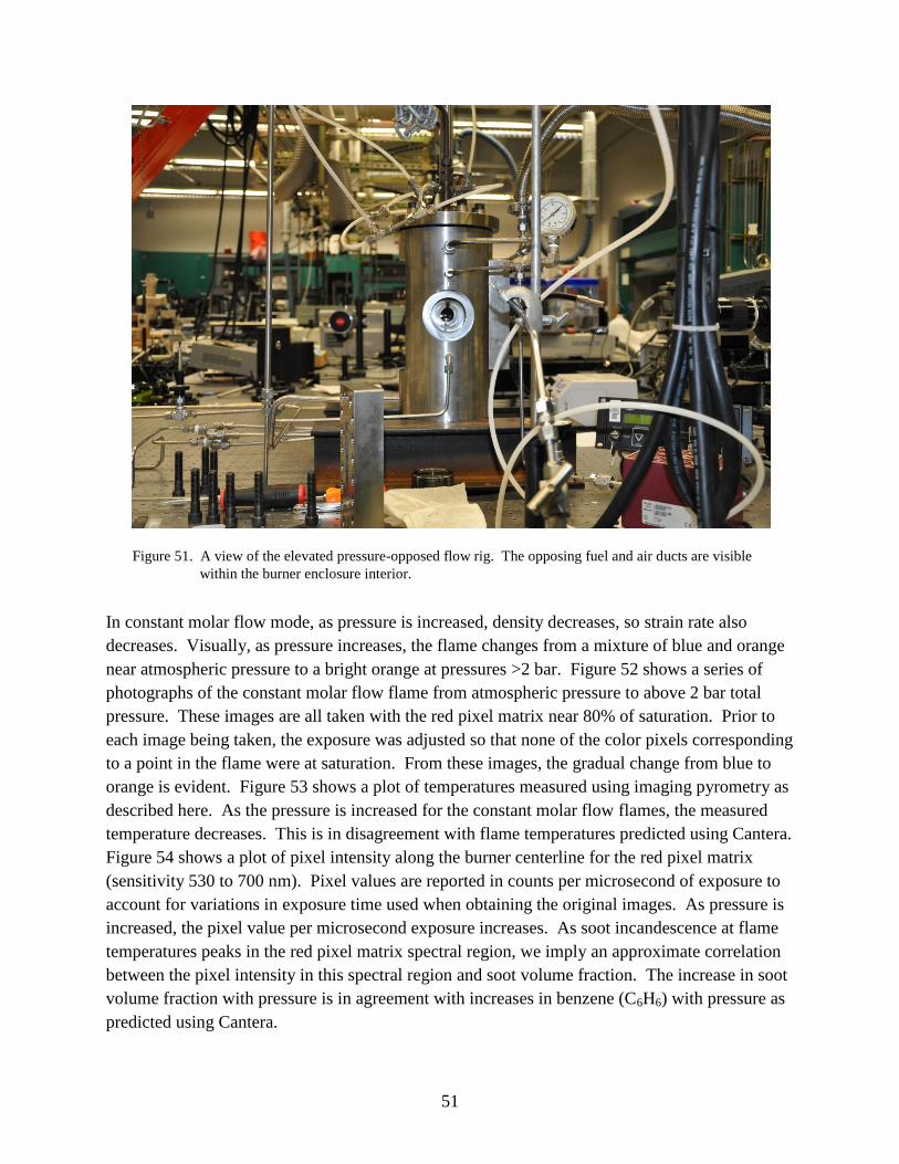
51
Figure 51. A view of the elevated pressure-opposed flow rig. The opposing fuel and air ducts are visible
within the burner enclosure interior.
In constant molar flow mode, as pressure is increased, density decreases, so strain rate also
decreases. Visually, as pressure increases, the flame changes from a mixture of blue and orange
near atmospheric pressure to a bright orange at pressures >2 bar. Figure 52 shows a series of
photographs of the constant molar flow flame from atmospheric pressure to above 2 bar total
pressure. These images are all taken with the red pixel matrix near 80% of saturation. Prior to
each image being taken, the exposure was adjusted so that none of the color pixels corresponding
to a point in the flame were at saturation. From these images, the gradual change from blue to
orange is evident. Figure 53 shows a plot of temperatures measured using imaging pyrometry as
described here. As the pressure is increased for the constant molar flow flames, the measured
temperature decreases. This is in disagreement with flame temperatures predicted using Cantera.
Figure 54 shows a plot of pixel intensity along the burner centerline for the red pixel matrix
(sensitivity 530 to 700 nm). Pixel values are reported in counts per microsecond of exposure to
account for variations in exposure time used when obtaining the original images. As pressure is
increased, the pixel value per microsecond exposure increases. As soot incandescence at flame
temperatures peaks in the red pixel matrix spectral region, we imply an approximate correlation
between the pixel intensity in this spectral region and soot volume fraction. The increase in soot
volume fraction with pressure is in agreement with increases in benzene (C6H6) with pressure as
predicted using Cantera.

52
Figure 52. Raw images of elevated pressure-opposed flow flames at constant molar flow rate taken using a
high-speed camera. It was necessary to adjust the camera exposure for each run to avoid
saturating the camera chip.
530 torr
5000 usec 6000 us
870 torr 968 torr
3000 usec
1000 usec
12 psi10 psi
2500 usec
15 psi
1000 usec
800 usec
20 psi
4 l/m ethylene2.7 l/m air

53
Figure 53. Peak centerline temperatures (K) for elevated pressure ethylene/air flames at constant molar flow and
at constant strain. Elevated pressure-opposed flow burner, ethylene/air flame. Temperatures are
calculated using images in figures 51 and 52.
Figure 54. Peak intensity per pixel per microsecond exposure along the burner centerline for the red pixel
matrices (570–700 nm) from images of elevated pressure-opposed flow ethylene/air flames.
0
500
1000
1500
2000
2500
3000
0.5 1 1.5 2 2.5 3
Pe
ak C
en
terl
ine
Te
mp
era
ture
(K
)
Pressure (Bar)
T (K) constant molar flow
T (K) constant strain
0
0.05
0.1
0.15
0.2
0.25
0.3
0.35
0.4
0.45
0 0.5 1 1.5 2 2.5 3
Inte
nsi
ty p
er
pix
el/
use
c (5
70
-70
0 n
m)
Pressure (Bar)
Constant molar flow
Constant strain

54
For constant strain mode, the flow rate of fuel and oxidizer gases was varied to account for
changes in gas density as pressure was increased. At atmospheric pressure, the initial flame was
based upon a flow rate of 2 L/min oxidizer and 2.9 L/min ethylene. At our burner configuration,
this resulted in a global oxidizer strain rate of 72 s–1
. To maintain this strain rate up to a total
pressure approaching 3 bar, the oxidizer flow rate was eventually raised to 5.4 L/min (with a
concurrent increase in fuel flow rates). Images of these flames measured using the same
methodology as for constant molar flow flames are shown in figure 55. As seen for constant
molar flow rate flames, the most notable visual change with increasing pressure was an increase
in luminosity as the flames changed from a mixture of blue and orange to bright orange.
Figure 53 shows the temperature decreasing with increasing pressure for the constant strain rate
flames. Figure 54 shows the 530- to 700-nm pixel intensity per microsecond exposure
increasing with pressure. At present, we have no explanation for the disagreement between
measured temperatures and those predicted using Cantera for either of the elevated pressure-
opposed flow flames reported here.
Figure 55. Raw images of elevated pressure-opposed flow flames at constant strain rate taken using a high-
speed camera. It was necessary to adjust the camera exposure for each run to avoid saturating
the camera chip.
450usec 750 us
25 psi 20 psi
3000 us
15 psi 10 psi
4000 us
1000 torr
3000 usec 4000 usec
749 torr 637 torr
4000 usec
Ethylene/air opposed flow flame – constant strain - Raw

55
3.7 Explosives Testing
An ideal explosive releases all of its energy instantaneously, allowing the explosive impulse at
any time or distance from charge center to be determined from pressure and temperature at time
zero (Kinney and Graham, 1985). However, as pointed out by Mader (2008), “All explosives are
non-ideal.” This means that chemical processes that influence explosive impulse and fireball
temperature can occur after explosive detonation at times later than predicted by standard
numerical codes (e.g., CHEETAH [Fried et al., 1998]). Traditional methods of measuring
explosive impulse and temperature are point measurements employing mechanical, piston-type,
piezo-based pressure transducers and thermocouples. Recently, measurements and calculations
performed at ARL suggest that the release of energy by nonideal explosives after initiation is
determined by product gas composition and temperature (McNesby et al., 2010). Therefore, to
accurately measure performance of nonideal explosives, it is necessary to map out pressure and
temperature fields immediately following initiation. Over the past several years, we have been
developing an optical approach that uses high-speed imaging to retrieve temperatures and
pressures from functioning explosives. Here, we summarize our efforts to date, using the high-
explosive formulation C-4 (94% trimethylene trinitramine [RDX, C3H6N6O6], remainder binder).
3.7.1 Theory
As mentioned previously, spectral intensity per unit wavelength Iλ can be determined through
Planck’s law (equation 13) (Planck, 1901). It states that spectral intensity is a function of
variables: wavelength λ, temperature T, and emissivity ελ, in addition to Planck’s constant h, the
speed of light in vacuum c, and the Boltzmann constant k.
1
125
2
kThc
e
hcI
.
(13)
In principle, temperature is determinable from a single intensity measurement at a known
wavelength. However, for a remote measurement made some distance away from the source, the
measured intensity will also be a function of geometry, light collection efficiency, instrument
transmission efficiency, and detector responsivity. Because of the practical difficulty in
accurately accounting for these complicating factors, two wavelength intensity measurements are
generally used to eliminate an arduous calibration (McNesby, 2005b). The temperature is thus
calculated from the ratio of intensities at two different wavelengths (equation 2). Upon
examination of equation 14, it is clear that an assumption must be made about emissivities ε1 and
ε2 to explicitly extract a temperature. The clear choice is to assume that the ratio of emissivities
is constant and unity. In other words, the fireball is assumed to behave as a graybody. Previous
work has shown this to be a valid assumption under a range of conditions (Levendis et al., 1992;
Panagiotou et al., 1996). However, for temperature measurements using emission from hot soot
particles, a wavelength-dependent emissivity correction is available (Murphy and Shaddix,
2004).

56
1
1
1
2
2
1
2
1
5
1
5
2
kThc
kThc
e
e
I
I
.
(14)
Wavelength-specific intensities measured by the photodiodes are modified by calibration
constant Ci to account for the previously disregarded variations in light collection geometry,
transmission efficiency, and detector responsivity. The calibration constant also compensates for
differing transmission widths of the band-pass filters, as long as the transmission width Δ λ is
small relative to λ 1 – λ 2. These factors are subsumed into a single calibration constant for each
photodiode. Thus, the ratio of any two measured intensities is expressed by equation 15. The
calibration constants C1,2 are determined through measurement of a calibration source at known
temperature.
2
1
2
1
2
1
IC
IC
S
S .
(15)
3.7.2 Wien’s Approximation
Equation 14 can be solved implicitly for temperature or explicitly by invoking Wien’s
approximation (equation 16) (Mehra and Rechenberg, 1982). Temperature may then be
expressed in terms of the known physical constants, wavelengths of interest, and detector signals
with calibration constants (equation 17).
kT
hckT
hc
ee 1 . (16)
12
1
2
21
lnln5ln
11
2
1
S
S
C
Ck
hcT . (17)
For wavelengths of interest used most often by us (i.e., 700, 820, and 900 nm), the maximum
error introduced by Wien’s approximation compared to the exact solution is 5% at a temperature
of 6000 K. However, a 5% error at 6000 K is not insignificant. Figure 56 compares the intensity
ratio and resulting error as a function of temperature.

57
Figure 56. (Top) Intensity ratio vs. temperature comparison of
Wien’s approximation and an exact solution. (Bottom)
Error vs. intensity ratio between Wien’s approximation
and an exact solution.
0
0.5
1
1.5
2
2.5
3
0 1000 2000 3000 4000 5000 6000 7000 8000
Temperature, K
I 900
nm/I
700
nm
.
exact Wien's approximation
-6
-5
-4
-3
-2
-1
0
0 0.5 1 1.5 2 2.5 3
I900 nm/I700 nm
Err
ror,
%
.

58
It is possible to improve upon the calculated temperature of equation 17 and still obtain an
explicit solution. By finding an appropriate correction function for the measured intensity ratio,
21
,, 21 IIC f , the error introduced by Wien’s approximation is able to be compensated by
using equation 18.
12
2,1
21
21
lnln51
,,ln
11
2
1
S
S
cC
k
hcT
f
. (18)
The error in intensity ratio shown in figure 56 is fit with a power-law profile for temperatures
below 6000 K (equation 19). Constants a and b are dependent on the particular values of λ 1 and
λ 2 and were determined for all wavelength combinations through a linear least-squares
regression curve fit. A corrected-temperature profile is determined from equation 18 using the
correction function containing the superposition of the intensity ratio and error (equation 20).
When this method is used, the previous 300-K error at 6000 K is reduced to <4 K.
b
I
Ia
2
1
. (19)
1
2
1
2
1
b
fI
Ia
I
IC
. (20)
Spectral intensity measurements at multiple wavelengths serve as a verification of the integrating
pyrometer’s performance and validity of the assumptions outlined previously. In this case,
independent temperature calculations are made by choosing different signal pairs and checked
for agreement. The choice of wavelengths is governed by four main factors:
1. Intensity ratio at selected wavelength pairs should exhibit a strong temperature
dependence.
2. Individual intensity should be as large as possible to maximize the signal-to-noise ratio.
3. Emissivity should not vary greatly over the wavelength range of interest.
4. Any discrete emission from the system under measurement should not coincide with the
wavelengths chosen for temperature calculation.
For the three-color integrating pyrometer, a system with wavelengths of 700, 820, and 900 nm
was used. Figure 57 shows the wavelength of peak-specific intensity vs. temperature, with a
maximum in the near-IR region at temperatures of 2000–4000 K. Thus, temperatures may be
calculated as just described using any two of the three available optical-pyrometer signals.

59
Figure 57. Wavelength of peak specific intensity vs. temperature.
An equivalent temperature calculated by all three pairs adds confidence to the measurement and
decreases the likelihood that errors in the calibration or equipment malfunction will go
undiscovered.
3.7.3 Experimental
Experiments were conducted at an outdoor test range at APG. The test range consisted of a
rectangular concrete deck, 2100 m2, surrounded by barricaded control buildings. The
experimental apparatus consisted of an explosives test rig and optical diagnostics test rig
separated at the center of the concrete deck by ~12 m. The explosives test rig was centered on a
1.5 m2 table positioned 0.84 m above the concrete deck. The table surface was an 8.26-cm-thick
steel plate. Explosive charges were suspended over the table center by nylon string at standoff
distances of 12.7, 19.0, 31.8, 44.4, and 63.5 cm. Detonation was initiated by an RP-83 exploding
bridge-wire detonator. Diagnostic instrumentation was triggered by rupturing an illuminated
600-μm Si core optical fiber placed adjacent to the charge apex. Upon explosive initiation, a
trigger pulse was generated due to the abrupt loss of light transmission through the fiber.
0
200
400
600
800
1000
1200
1400
1600
0 2000 4000 6000 8000
Temperature, K
(I
max)
, n
m
.

60
The multi-imaging rig consists of four separate instruments: a three-color integrating pyrometer,
a two-camera imaging pyrometer, a full-color single-camera pyrometer (Densmore et al., 2011),
and a wavelength-resolved spectrograph (300–800 nm). Each pyrometer in the imaging rig
operates on the same scientific principle: determining temperature from spectral emission
intensity. The rig was enclosed in 1- × 1- × 2-m-tall armored enclosure (2.54-cm-thick steel)
with an ~30 cm2 viewing port positioned 1.22 m off the concrete deck. The viewing port was
uncovered to prevent the need to calibrate the pyrometers through window material and also
because there was no anticipated fragment danger from the uncased C-4 charges. A diagram of
the full test rig setup is shown below in figure 10.
3.7.4 Three-Color Integrating Pyrometer
Figure 58 shows a schematic of the three-color integrating optical pyrometer. This pyrometer rig
has the fastest time response of the pyrometer setups used here but the poorest spatial resolution.
The fixture aiming the three optical fibers at the center of the fireball is made of steel and was
specially designed for this rig in order to keep the center of line of sight of the three optical fibers
parallel.
Figure 58. Schematic of the three-color integrating pyrometer rig.
Emission from explosionFace plate
Fiber optic cables
Narrow bandpass filters
Si Photodetectors
To data acquisition
Emission from explosionFace plate
Fiber optic cables
Narrow bandpass filters
Si Photodetectors
To data acquisition
Emission from explosionFace plate
Fiber optic cables
Narrow bandpass filters
Si Photodetectors
To data acquisition
Emission from explosionFace plate
Fiber optic cables
Narrow bandpass filters
Si Photodetectors
To data acquisition

61
The three-color integrating optical pyrometer consists of three silicon-based photodiodes
(Thorlabs model DET 210), three 10-nm band-pass filters, and Si-Si fiber optic cables (22°
acceptance angle) to couple light from the event to the detectors. The pass bands of the filters
were centered at 700, 820, and 900 nm. These wavelengths were chosen to provide optimal
sensitivity in the temperature range of 2000–4000 K. The resulting voltage output from each
photodiode is recorded directly on a digital oscilloscope. Data acquisition is triggered by the
same signal used to initiate the explosive train.
Fireball emission is coupled into the fiber optics without any focusing optics. Thus, the fiber
optics collect light from a broad spatial region. Since high-temperature regions of the fireball
exhibit higher intensity (Gaydon, 1941), the temperature measured by the pyrometer is biased
toward the hottest portion of the visible surface. Little temperature information is gained from
the fireball interior as the fireball gases are optically thick; therefore, radiation from the interior
is effectively shielded from view by the outer layers. This caveat also pertains to temperature
measurements by the camera-based pyrometers, i.e., reported temperatures are surface
temperatures.
Calibration is typically performed with a well-characterized calibration lamp. However, working
under ambient conditions in the field presents difficulties in keeping calibration instrumentation
performing per its specifications. As a result, the sun was used as an alternate radiation source.
The sun is a nearly ideal blackbody source with a temperature of 5900 K (ASTM, 2003).
However, absorption by the atmosphere alters the spectral intensity received at ground level. A
comparison of solar irradiance with an ideal blackbody is shown in figure 59 (ASTM, 2003).
The chosen wavelengths were away from major water absorption lines to decrease the variability
in the calibration due to changes in atmospheric water vapor concentration.
3.7.5 Two-Color Imaging Pyrometer
The two-color imaging pyrometer employs two Vision Research Phantom 5.1 monochrome
cameras that image the explosive event along a single optical axis. A schematic of the two-color
imaging pyrometer is shown in figure 60. Focusing was accomplished using a single lens and
beam splitter assembly. The cameras were synched to a common time base by using one as the
“master,” which receives the trigger pulse and relays it to the second camera, the “slave.”
Cameras were fit with 10-nm narrow band-pass filters at 700 and 900 nm. The locations of the
filtered wavelengths relative to a blackbody at 2000 K are also shown in figure 60. System
resolution is dictated by the fixed effective focal length of the collection optics. Therefore, the
field of view (FOV) is adjusted by selecting the number of pixels in the image. The FOV must
be balanced with both the frame rate and exposure to ensure adequate signal-to-noise ratio. The
exposure time was the limiting factor in the camera setup due to the narrow band pass and
colinear optical-axis design. Cameras were set to 5000 frames/s and 196-μs exposure, with an
image size of 448 × 200 pixels. This rig was designed in-house.

62
Figure 59. Comparison of solar radiation both outside the atmosphere and at sea level with
emission from an ideal blackbody at 5900 K. The baselines have been shifted for
clarity.
Solar irradiance
0
0.5
1
1.5
2
2.5
3
3.5
0 500 1000 1500 2000 2500
wavelength, nm
W/m
2n
m
.
5900 K black body
solar radiation,
exo-atmospheric
solar radiation,
sea level

63
Figure 60. (Top) Schematic of the single-axis two-color imaging pyrometer showing the lens and
beam splitter arrangement. (Bottom) Band pass of each camera superimposed upon the
emission from a blackbody near 2000 K.
The experimental setup included a mechanism and procedure to precisely align the images from
both cameras. The procedure was repeated before each test to ensure that the passing blast wave
did not disturb the alignment. In addition, calibration images were saved to verify the alignment
offline. These images could be used to correct pixel registration but were deemed unnecessary.
Temperature calibration was achieved by recording images of a commercial blackbody source at
1255 K (Omega Engineering).
Video 1
Video
2
Filter 900nm
Filter 700 nmBeamsplitter
Lens Assembly
0
0.2
0.4
0.6
0.8
1
400 600 800 1000 1200
Wavelength (nm)
Black Body
700nm filter
900nm filter

64
3.7.6 Full-Color Imaging Pyrometer
The full-color imaging pyrometer, discussed in detail in section 2.3, uses the Bayer-type mask to
generate wavelength-specific emission data from a single camera (here, a Vision Research
Phantom 5.1 color camera) (Densmore et al., 2011). The advantage of this technique is that any
error associated with pixel registration between wavelength-specific images is virtually
eliminated. The disadvantage is that significant errors may be introduced if there is strong
discrete emission (e.g., for hydrocarbon/air flames, strong C2 or CH emission from nonsooting
flames). The Bayer-type mask generates subpixel output in red, green, and blue spectral regions
for each frame recorded by the camera. A MATLAB program generates the three separate pixel
arrays from each frame and ratios them pixel by pixel to create a 2-D temperature map from each
frame. A temperature movie is then created from the individual temperature maps.
In principle, any color camera with a digital readout may be used for temperature imaging,
provided something is known about any camera specific “on-chip” image processing. However,
each camera must go through a tedious calibration to map out the pixel response across the full
visible spectrum (Densmore et al., 2011). Camera calibration involves comparing subpixel
output with the output from a calibrated photomultiplier tube for narrow bandwidth radiation
over the full visible spectrum. Figure 61 shows a schematic of the Bayer-type mask in front of
the sensor element of a typical color camera and the resulting calibration graph for the camera
used in these measurements.
3.7.7 Wavelength-Resolved Emission Spectrograph
An often overlooked aspect of reacting systems pyrometry is the importance of discrete emission
(McNesby et al., 2004). As an example, figure 62 shows wavelength-resolved emission from
three types of ethylene/air diffusion flames (McNesby, 2005b). Most emission pyrometry
measurements assume a blackbody-like emitter with an emissivity that is invariant with
wavelength but less than unity; this is known as the graybody assumption (Planck, 1914).
However, as shown in figure 62, diffusion flames may show near-graybody behavior (the candle-
like flame) or a mixture of graybody and discrete emission (the coflow flame labeled “diffusion
flame”). They also may be nearly particulate free, in which case the emission is virtually all
from molecular and atomic emission (the opposed-flow diffusion flame labeled OPPDIF, which
shows little flame emission other than discrete C2 and CH band emission). Because this discrete
emission occurs in the visible (300–800 nm) and IR (1–30 μm) spectral regions, it presents the
greatest error source for the full-color imaging pyrometer. For this reason, a wavelength-
resolved emission spectrum is measured during every experiment using a fiber-coupled
spectrograph (Ocean Optics HR 4000, 1-nm resolution). The spectrograph collects and disperses
light for 50 ms following the received trigger. The reported spectrum will show any discrete
emission but does not tell when during the 50-ms collection window the emission occurred.

65
For results reported here, the graybody assumption was assumed to hold. As mentioned
previously, emissivity corrections for the most common particulate emitter (soot) have been
published in the open literature (Murphy and Shaddix, 2004). The explosive used here
(Composition C-4) is considered oxygen balanced, and the chemical makeup of the detonation
products is not known from experiment. Thus, wavelength-dependent emissivity corrections are
not employed here.
Figure 61. (Top) Schematic of the full-color imaging pyrometer showing the Bayer-type mask in front of the
sensor chip. (Bottom) Pixel calibration example from a Vision Research Phantom 5.1 camera.

66
Figure 62. (Top) Wavelength-resolved emission for three types of ethylene/air flames. (Bottom) Detail of emission from the OPPDIF flame showing emission bands due to CH and C2.
0
500
1000
1500
2000
2500
3000
3500
300 400 500 600 700
Wavelength (nm)
Em
issi
on
In
ten
sity
(a.
u.)
C2H4 candle
C2H4 diffusion flam e
OPPDIF C2H4-air
100
150
200
250
300
350
400
300 400 500 600 700
Wavelength (nanometers)
Em
issi
on
Inte
nsi
ty (
arb
.un
its)
C2 (Swan)
CH

67
3.7.8 Explosive Charges
Thirty-two spherical C-4 charges were exploded (twenty-nine 227-g charges and three 454-g
charges), and fireball temperature was measured using the multi-imaging rig. Five standoff
distances were used: three 12.7-cm charges, six 19.0-cm charges, six 31.8-cm charges, nine
44.4-cm charges (six 227-g charges and three 454-g charges), and eight 63.5-cm charges. Data
from three charges were incomplete due to either equipment malfunction or operator error. Only
three charges at a 12.7-cm standoff were measured, as other equipment (not reported here) was
damaged at this standoff distance. Based upon charge-to-charge variance within a test method,
we estimate temperature measurements reported here to have an uncertainty of between +/–100
K (integrating pyrometer, full-color pyrometer) to +/–200 K (two-color pyrometer).
3.7.9 Results: Three-Color Integrating Pyrometer
Figure 63 shows a typical raw data record from the three integrating photodiodes for the first
25 ms following initiation. The signals are a result of the fireball emission directed onto the
600-μm core Si-Si optical fiber and focused onto the surface of the photodetector. Because the
optical fiber possesses a 22° acceptance angle, spectral emission is received from all regions of
the fireball, hence the nomenclature of an integrating pyrometer. Spectral emission levels fall
below the noise threshold at ~100 ms for all three wavelengths.
Figure 63. Raw three-color integrating pyrometer data for a 227-g spherical C-4 charge, 19.0-cm standoff.
0.00E+00
1.00E-02
2.00E-02
3.00E-02
4.00E-02
5.00E-02
0 0.005 0.01 0.015 0.02 0.025
Time (seconds)
Inte
nsit
y (
a.u
.)
700 nm
820 nm
900 nm

68
Blackbody power output is governed by the Stefan-Boltzman law (equation 21) (Mehra and Rechenberg, 1982). Where W is the blackbody power output over all wavelengths, T is absolute temperature, A is the radiating surface area, and σ is the Stefan-Boltzmann constant. Because power output is proportional to the fourth power of temperature, the reported intensities will possess a larger contribution from hotter regions of the fireball. Therefore, the temperature calculated using the three-color pyrometer will be more indicative of a peak fireball temperature rather than an average fireball temperature.
4ATW . (21)
Three possible intensity ratios, and hence three possible temperature calculations, exist for the three-color integrating pyrometer: I700 nm/I820 nm – T12, I820 nm/I900 nm – T23, and I700 nm/I900 nm – T13. These three temperature calculations would be in reasonable agreement for a well-behaved experiment. In practice, however, T23 is generally in poorest agreement with the other calculated temperatures. This may be because the T23 temperature ratio possesses the smallest wavelength difference between factors in the calculation. Figure 64 shows the three calculated temperatures as a function of time for the raw data of figure 63. Additionally, the average calculated temperature profile is shown in figure 64. From here on, the remaining temperature data reported are the average calculated temperatures from the three intensity ratios.
Figure 64. (Left) Calculated three-color integrating pyrometer temperatures for a 227-g spherical C-4 charge at 19.0-cm standoff. (Right) Average temperature profile from the three calculated temperatures.
In what follows, standoff refers to the distance between the center of the unexploded charge to the table surface. As shown by figure 64, the highest temperature recorded occurs immediately after detonation. This is followed by an approximately exponential decay lasting 2 ms to a nearly constant temperature of 1/e times the initial temperature value. This constant temperature persists out to 100 ms, where the intensity signal eventually falls below the noise threshold. All charges detonated exhibited this same overall trend.
-200
1800
3800
5800
7800
9800
0 0.005 0.01 0.015 0.02
Time (seconds)
Te
mp
era
ture
(K
)
T12
T23
T13
0
2000
4000
6000
8000
0 0.005 0.01 0.015 0.02
Time (seconds)
Te
mp
era
ture
(K
)
-200
1800
3800
5800
7800
9800
0 0.005 0.01 0.015 0.02
Time (seconds)
Te
mp
era
ture
(K
)
T12
T23
T13
0
2000
4000
6000
8000
0 0.005 0.01 0.015 0.02
Time (seconds)
Te
mp
era
ture
(K
)

69
In general, the three-color integrating pyrometer displayed good repeatability in measured
temperatures, with most charges varying by only a few percent of each other at all times. For all
227-g charges measured (29 total), calculated temperatures at a given standoff differed by <10%
at any time. Figure 65 shows temperature calculations for the 227-g charges detonated at a
standoff of 19.0 cm. This data set possessed the largest measured temperature variance using the
three-color integrating pyrometer of all standoff distances studied.
Figure 65. Average three-color integrating pyrometer calculated temperature profile for a 227-g spherical C-4
charge at 19.0-cm standoff.
Figure 66 illustrates the time varying temperature calculated with the three-color integrating
pyrometer at a specified charge standoff distance. As shown, the middle-time (1–5 ms after
initiation) temperature decreases with increasing charge standoff. The quantity of thermal
radiation reflected off of the steel table and back into the fireball increases with decreasing
standoff distance, resulting in an increase of middle-time temperatures. Lastly, figure 66
illustrates that all temperature profiles decay to the same final temperature within 10 ms.
0
1000
2000
3000
4000
5000
6000
7000
0 0.005 0.01 0.015 0.02
Time (seconds)
Tem
pera
ture
(K
)
7.5 inch standoff shot 1
7.5 inch standoff shot 2
7.5 inch standoff shot 3
7.5 inch standoff shot 4
7.5 inch standoff shot 5

70
Figure 66. Average temperature profile calculated from all charges at a specified standoff distance with the
three-color integrating pyrometer.
Figure 67 shows the three-color integrating pyrometer temperature profiles for the 454-g charges
compared to the 227-g charge average at the same standoff. Of these, two charges produced
higher middle-time temperatures than the 227-g charges. This is expected, as the larger charges
yield twice the energy of the 227-g charges and therefore exhibit a longer energy dissipation
time, yielding higher temperatures at later times. The third charge produced a temperature
profile similar to that of the 227-g charges at the same standoff distance.
2000
2500
3000
3500
4000
4500
5000
5500
6000
0 0.001 0.002 0.003 0.004 0.005 0.006 0.007 0.008 0.009 0.01
Time (seconds)
Te
mp
era
ture
(K
)
25 inch standoff - 7 shots
17.5 inch standoff - 4 shots
12.5 inch standoff - 4 shots
7.5 inch standoff - 5 shots
5 inch standoff - 2 shots

71
Figure 67. Average three-color integrating pyrometer calculated temperature profile for the three 454-g
spherical C-4 charges at 44.4-cm standoff distance, compared to the average temperature profile
from the 227-g charges at that standoff.
3.7.10 Results: Two-Color Imaging Pyrometer
Image pairs from the two cameras were ratioed pixel by pixel using a similar algorithm described
for the three-color integrating pyrometer. However, the filters used limited the light reaching the
camera sensors. This necessitated longer exposure times and limited the time resolution of this
technique. Due to the limited number of images obtained using the two-color imaging
pyrometer, temperatures were determined by performing a numerical search of the full Planck
equation ratio assuming constant emissivity (equation 14). Composite 2-D temperature maps
and movies were created in-house using MATLAB software.
Figure 68 shows four resulting temperature maps from the detonation of a 227-g charge at an
initial charge standoff distance of 63.5 cm. Images were recorded at 5000 frames/s with an
exposure time of 196 μs. The FOV was ~0.76 × 1.52 m. The total time duration covered by the
four images was 1 ms. Each false-colored temperature map is accompanied by a corresponding
color bar scale and temperature histogram. Color frequency is proportional to temperature, i.e.,
yellow is hotter than red. The most prevalent temperature per image decreases from 2500 to
1500 K as the fireball size increases.
0
1000
2000
3000
4000
5000
6000
7000
0 0.002 0.004 0.006 0.008 0.01
Time (seconds)
Te
mp
era
ture
(K
)
3rd 1 lb
2nd 1 lb
1st 1 lb
0.5 pound

72
Figure 68. Two-camera imaging pyrometer calculated temperature maps and corresponding histograms. Time
sequence: a < b < c < d. The fireball reaches full size sometime between temperature maps a and b.
Temperatures map (a) shows the first image captured after detonation, where the fireball is ~50%
of its final size with peak temperatures approaching 4000 K. The remaining temperature maps
show the fireball temperature decays as it nears full size. A distinct feature of these maps is the
hot outer-fireball surface. This will be discussed in the full-color imaging pyrometer section
(3.7.11).
Figure 69 shows the measured gas temperature at the steel table surface (63.5 cm from charge
center) using the two-color imaging pyrometer as a function of time for the 227-g charge from
figure 68. The data exhibits the previously mentioned exponential temperature decay within the
first millisecond after the expanding fireball reaches the table surface. However, the temperature
at 5 ms is considerably lower than that measured using the three-color integrating pyrometer.
3.7.11 Results: Full-Color Imaging Pyrometer
As briefly discussed in section 2.3, figure 26 shows measured gas temperature maps from the
full-color imaging pyrometer for a charge similar to that shown in figure 68 (227-g charge at a
63.5-cm standoff). The interframe time is 71 μs, corresponding to a camera framing rate near
14,000 frames/s. Temperature maps are accompanied by a corresponding color-bar scale.
a b
c d
a b
c d

73
Figure 69. Calculated gas temperature at the steel table surface using the two-color imaging pyrometer for the
charge shown in figure 68.
Temperature maps represent the event being viewed from the side, similar to the view of the
two-camera imaging pyrometer. The apparent heating of the table is a result of reflection of
thermal radiation by the table surface.
A hot outer-fireball surface is visible in the full-color imaging pyrometer temperature maps (e.g.,
figure 26). This edge heating is hypothesized to indicate the primary shock wave location. The
passage of a shock wave results in a discontinuous jump in thermodynamic properties, one
property being the temperature (Kinney and Graham, 1985). Thus, the strong primary shock
wave associated with the range of radial fireball measurements imaged generates a few hundred
Kelvin increase in temperature. Secondly, the primary shock wave is known to coincide with the
outer-fireball surface at tens of charge diameters (McNesby et al., 2010). Thus, the few hundred
Kelvin increase in temperature shown over the range of fireball radii measured supports the
hypothesis that the hot outer-fireball surface is indicative of the primary shock wave location.
1500
1600
1700
1800
1900
2000
2100
2200
2300
2400
2500
0 0.0005 0.001 0.0015 0.002 0.0025 0.003 0.0035 0.004 0.0045 0.005
Time (seconds)
Tem
pera
ture
(K
)

74
Figure 70 is a plot of temperature at the steel table surface vs. time for the 227-g charges at the
five standoff distances studied. The data were extracted from the full-color pyrometer
temperature images. The plot illustrates that the steel table surface experiences high
temperatures as a result of contact with hot gases. Gases at the steel table surface cool to the
bulk fireball temperature (~2000 K) within 0.5 ms. As expected, figure 70 shows that a slight
time lag exists between detonation and the increased gas temperature at the steel table surface for
charges at the largest standoff.
Figure 70. Full-color pyrometer extracted gas temperatures at the steel table surface vs. time for 227-g C-4 charges
at the five standoff distances.
Figure 71 is a graph of gas temperature at the steel table surface vs. time for the 227- and 454-g
charges at a standoff of 44.4 cm. The data were extracted from the full-color pyrometer
temperature images. The key difference between the two sets of data is the increase in peak gas
temperature for the 454-g charge compared to the 227-g charge.
1500
1600
1700
1800
1900
2000
2100
2200
2300
2400
2500
0 0.0005 0.001 0.0015 0.002 0.0025 0.003 0.0035 0.004 0.0045 0.005
Time (seconds)
Tem
pera
ture
(K
)
25 inch standoff
17.5 inch standoff
12.5 inch standoff
7.5 inch standoff
5 inch standoff

75
Figure 71. Gas temperatures at the steel table surface for the 227- and 454-g charges at a standoff of 44.4 cm.
3.7.12 Optical-Pressure Measurement
Peak shock wave pressure Ps of an expanding spherical shock wave is determined from knowing
the shock wave Mach number M and atmospheric pressure Pa through the use of the Rankine-
Hugoniot relationship (equation 22) (Kinney and Graham, 1985). When sequential images of the
expanding fireball/primary shock wave are used, a profile of shock wave radius as a function of
time can be measured. Taking the derivative of this profile with respect to time yields a profile
of shock wave velocity as a function of shock wave radius. Dividing the shock wave velocity by
the known atmospheric speed of sound, a profile of shock wave Mach number as a function of
shock wave radius is determined, permitting the calculation of a peak shock wave pressure from
equation 22. Figure 72 shows the average optically measured peak shock wave pressure at the
steel table surface for the 227-g charges at the five standoff distances measured in these
experiments. Each data point is an average of the peak shock wave pressure measured for all
charges at a particular standoff distance.
1500
1700
1900
2100
2300
2500
2700
0 0.0005 0.001 0.0015 0.002 0.0025 0.003 0.0035 0.004 0.0045 0.005
Time (seconds)
Tem
pera
ture
(K
)
1 pound
1/2 pound

76
Figure 72. Average optically measured peak shock wave pressure at the steel table surface for the 227-g C-4
charges at the five standoff distances measured.
176
1 2 MP
P
a
s . (22)
3.7.13 Wavelength-Resolved Emission Spectrograph
As was shown by figure 62, it is necessary to measure the wavelength-resolved emission
spectrum when using any emission pyrometry technique. When discrete spectral features
become as or more intense than graybody emission, the calculated emission pyrometer
temperatures may be in error. Thus, for each charge tested, the wavelength-resolved emission
spectrum was measured. Figure 73 shows the emission spectrum for the charge shown in figure
15 (227 g at 63.5-cm standoff). Only one emission spectrum is reproduced here, as the emission
spectra for all charges tested were similar. The dominant discrete spectral feature was the
sodium emission lines near a wavelength of 589 nm. Therefore, the sodium lines would be a
systematic source of error for the full-color pyrometer temperature measurements. Because this
feature represents a small contribution (~1%) of the measured graybody intensity, the presence
of this emission feature introduces negligible error in the temperature calculations. Therefore, no
attempt was made to correct for the error introduced by the sodium emission.
0
500
1000
1500
2000
2500
3000
3500
4000
0 5 10 15 20 25 30
Charge Standoff (inches)
Pre
ss
ure
at
Ta
ble
Su
rfa
ce
(p
si)

77
Figure 73. Emission spectrum for the charge shown in figure 15 (227 g of C-4 at 63.5-cm standoff).
The feature (doublet) near 589 nm is from sodium (Na) emission.
3.7.14 Discussion
Figure 74 reports particle temperatures measured from a 227-g charge using each method for the
test shown in figure 69. The charge was suspended 63.5 cm above the steel table surface. The
three-color pyrometer rig data shows the peak fireball temperature integrated over the full
fireball surface, while the two- and full-color pyrometer data shown are measured gas
temperatures at the steel table surface. The peak measured temperature by the two-color
pyrometer was ~2500 K and occurred 0.10 ms after initiation, or the time it takes for the
leading edge of the fireball to reach the table surface. The temperature continues to decrease to a
steady-state temperature near 1500 K, ~400 K below that reported by the three-color pyrometer.
The initial temperature change reported by the full-color pyrometer is in reasonable agreement
with that reported by the two-color pyrometer. However, at later times, there is a large
discrepancy between temperatures reported at the steel table surface by the two- and full-color
rigs. The full-color pyrometer does report a final temperature in good agreement with that
reported by the three-color pyrometer, ~2000 K. The two-color pyrometer signal-to-noise ratio
at later time measurements was the poorest of any method used here (~3:1). Based upon shot-to-
shot variation within a pyrometer type, we estimate the uncertainty in reported temperatures for
the three-color and full-color rigs to be ±100 K and the uncertainty in the two-camera system to
be approximately ±200 K.
0
100
200
300
400
500
600
300 400 500 600 700
Wavelength (nanometers)
Em
issio
n In
ten
sit
y (
arb
. u
nit
s)

78
Figure 74. Temperatures measured for a 227-g C-4 charge at 63.5-cm standoff using each pyrometry method.
Peak fireball surface temperatures measured immediately following detonation varied between
3000 and 5000 K and rapidly decayed to a steady-state temperature near 2000 K. The variability
in peak fireball surface temperature may be a result of the discrepancy in timing of the initial
frame relative to the time of detonation as data collection was triggered by the rupture of a fiber
placed near the charge apex. The steady-state temperature often observed for late time after
detonation (McNesby et al., 2005a) is hypothesized to be governed by fireball burning in the
case of fuel-rich explosives or slow cooling of detonation product gases for oxygen-balanced
explosives. Cooling of the rapidly expanding detonation product gases coupled with the initial
uncertainty in time measurement causes the first temperatures reported to show considerable
variance. Additionally, temperatures measured from emission spectra are calculated on the
assumption that the emitting particles are in local thermodynamic equilibrium. This assumption
may not hold for times close to detonation (Gaydon, 1974).
The examination of measured three-color pyrometer temperatures showed that for charges
closest to the steel table surface, the bulk fireball temperature exhibited higher initial
temperatures while also decaying slower than charges at greater standoff distances. For charges
at the smallest standoff distances, the early-time bulk fireball temperatures were up to 500 K
higher. This is attributed to the steel table surface reflecting a larger quantity of thermal
0
500
1000
1500
2000
2500
3000
3500
4000
4500
5000
0 0.0005 0.001 0.0015 0.002 0.0025 0.003 0.0035 0.004 0.0045 0.005
Time (seconds)
Te
mp
era
ture
(K
)
Three Color - Fireball Peak
Temperature
Two Color - Temperature at Metal
Surface - 25 in. Standoff
Full Color - Temperature at Metal
Surface - 25 in. Standoff

79
radiation from the fireball, effectively containing one side of the fireball. At later times,
regardless of charge standoff, the measured bulk fireball temperature decayed to a common value
near 2000 K.
Two- and full-color imaging pyrometer temperature measurements showed that gases at the steel
table surface reached a maximum temperature at approximately the same time the fireball made
contact with the surface. Within 0.5 ms of detonation, gases at the steel table surface had
reached the bulk fireball temperature. However, at later times, the two-color pyrometer rig
reported steady-state temperatures up to 400 K less than those reported for the full-color
pyrometer. We believe the main source of discrepancy between measurements made with the
two- and full-color rigs has to do with the loss of signal intensity at later times for the 900-nm
channel of the two-color rig. We are currently modifying our two-color rig to allow for greater
light throughput in this spectral region.
Fireball edge/primary shock wave expansion-rate measurements were obtained from the
full-color pyrometer images. Previous work has shown that the primary shock wave remains
attached to the outer surface of the rapidly expanding detonation products at distances up to tens
of charge diameters (McNesby et al., 2010). From these images, measured peak shock wave
velocities approached 4 km/s (4 mm/μs). Using the primary shock wave velocities with the
Rankine-Hugoniot relations, we found that peak shock wave pressures near the steel table
surface ranged from 1.38 to 24.82 MPa. An approximate inverse relationship was found
between charge standoff distance and peak shock wave pressure at the steel table surface.
3.7.15 Conclusion
This part of the report discusses the two methods we developed (two- and full-color pyrometry)
to map temperatures at early time following initiation of nonideal explosives, compares these to
each other, and compares them to the more common integrating pyrometer technique.
Temperature maps measured using the newer techniques are compared to those measured using
more conventional, integrating pyrometry. We believe that each method has utility in measuring
explosive performance. We find the integrating technique most useful in comparing a series of
explosives tests, as the setup is simple and the analysis straightforward. After using the integrating
pyrometer rig for several years, we found the most important maintenance to be a recalibration
before every test series. Using this technique, we have measured repeatable temperatures for
similar explosives when test dates were separated by over 1 year. However, when the integrating
pyrometer rig is used, the reported temperatures contain no spatial information; this may be
misleading when used to judge nonideal explosive behavior.
The two-color (two-camera) technique is valuable in that it potentially can overcome any
problems caused by discrete emission. Unfortunately, in the experiments reported here, we
believe late time temperature measurements are in error because of poor throughput in one of the
optical channels. We are currently working to overcome this problem.
80
The full-color method is possibly most intriguing because it potentially may be employed with
any color camera. Disadvantages include errors in measured temperatures from discrete
emission and possible nonlinearity issues for certain cameras near saturation. However, the full-
color rig (and to some extent the two-color rig) can map peak shock temperature by measuring
the Mach number of the fireball expansion. Together, the techniques reported here provide the
ability to map in early time the performance of a nonideal explosive and may help provide
insight into controlling dynamic energy release in new energetic materials. We are currently
working to address the discrepancies between reported temperatures but believe these
techniques, or similar techniques based upon high-speed imaging, are the key to evaluating
energetic materials in dynamic environments.
4. Pending Efforts
Our main pending effort involves resolving some questions about numerical simulations of
opposed flow flames that we reported on in Combustion and Flame (McNesby et al., 2005b),
pertinent to the SERDP-funded project reported here. Specifically, our model (and experiment)
predicted increases in soot when ethanol was added to the fuel side of an opposed flow
ethylene/air flame at 1-atm total pressure. More recently, a numerical simulation employing a
slightly different chemical mechanism of a coflowing ethylene/air diffusion flame to which
ethanol was added suggested that our proposed route to soot formation for fuel side ethanol
addition was incomplete (McEnally and Pfefferle, 2007).
In comparing that chemical mechanism to the model used by our group, we found that the
reaction
C3H3 + CH3 (+ M) --> C4H612 (+ M) (R2)
for the formation 1,2-C4H6 was exclusive to our chemical mechanism. When ethanol is added to
the fuel stream of the opposed flow burner, it is anaerobically pyrolyzed prior to flame region.
The pyrolysis products are C2H4, H2O, CH2OH, CH3, and lesser amounts of OH and C2H5 (~8%
of the amount of ethanol added). In our analysis, the reaction leading to increased A1 (C6H6,
benzene) production (and hence soot) is
n-C4H5 + C2H2 = A1 + H . (R3)
Since an acetylene bath is present within the flame region, the measured and predicted increase
was postulated to be from higher levels of n-C4H5. Our approach was to find a pathway to
increased levels of n-C4H5 that involved CH3 (the only anomalous product of ethanol pyrolysis).
n-C4H5 is involved in interconversion with i-C4H5,C4H4, C4H612, and C4H6. A rate of
production analysis for these species for the doped vs. neat flame yielded the reaction

81
C3H3 + CH3 (+M) = C4H612 (+M) . (R4)
Our approach to better understand soot formation involves combining our acetylene
measurement with a method for measuring the propargyl radical (C3H3). Our approach is to use
an external cavity QCL (Daylight Solutions) to measure the ν3 combination band near 1940 cm–1
(Jochnowitz et al., 2005). We plan to do a feasibility study using this technique to measure
propargyl radical formed by the thermal decomposition of propargyl bromide (Minsek and Chen,
1990).

82
5. References
Adams, J. E., Jr. Interactions Between Color Plane Interpolation and Other Image Processing
Functions in Electronic Photography. SPIE 1995, 2416, 144–151.
Adams, J. E., Jr. Design of Practical Color Filter Array Interpolation Algorithms for Digital
Cameras. SPIE 1997, 3028, 117–125.
Appel, J.; Bockhorn, H.; Frenklach, M. Kinetic Modeling of Soot Formation With Detailed
Chemistry and Physics: Laminar Premixed Flames of C2 Hydrocarbons. Combustion and
Flame 2000, 121 (1–2), 122–136.
ASTM G 143-03. Standard Tables for Reference Solar Spectral Irradiances: Direct Normal and
Hemispherical on a 37° Tilted Surface. Annu. Book ASTM Stand. 2003.
Bardin, F.; McBride, R.; Moore, A.; Morgan, S.; Williams, S.; Jones, J.; Hand, D. Real Time
Temperature Measurement for Process Monitoring of Laser Conduction Welding.
Proceedings of the 23rd International Congress on Applications of Lasers and Electro-
Optics, San Francisco, CA, 2004.
Bayer, B. E. Color Imaging Array. U.S. Patent 3 971 065, 1976.
Commission on Illumination (CIE) Web site. http://www.cie.co.at/ (accessed 20 September
2010).
Cooper, P. Explosives Engineering; Wiley-VCH: New York, 1996.
De Iuliis, S.; Barbini, M.; Benecchi, S.; Cignoli, F.; Zizak, G. Determination of the Soot Volume
Fraction in an Ethylene Diffusion Flame by Multiwavelength Analysis of Soot Radiation.
Combustion and Flame 1998, 115, 253.
Densmore, J. M.; Biss, M. M.; Homan, B. E.; McNesby, K. L. High Speed Digital Color Imaging
Pyrometry. Applied Optics 2011, 50 (17), 2659–2665.
DeWitt, D. P.; Nutter, G. D. Theory and Practice of Radiation Thermometry; John Wiley &
Sons: New York, 1988.
Dunlap, J. C.; Bodegom, E.; Widenhorn, R. Correction of Dark Current in Consumer Cameras.
J. Electronic Imaging 2010, 19 (1), 013010.
Duxbury, G.; Langford, M.; McCulloch, M. Rapid Passage Induced Population Transfer and
Coherences in the 8 Micron Spectrum of Nitrous Oxide. Molecular Physics 2007, 105 (5–7),
741–754.

83
Finlayson, G. D.; Hordley, S.; Hubel, P. M. Recovering Device Sensitivities With Quadratic
Programming. Proceedings of the Sixth Color Imaging Conference: Color Science, Systems
and Applications, Scottsdale, AZ, November 1998; p 90.
Fried, L. E.; Howard, W. M.; Souers, P. C. CHEETAH 2.0 User’s Manual; Lawrence Livermore
National Laboratory Report UCRL-MA-117541, Rev. 5; Lawrence Livermore National
Laboratory: Livermore, CA, 1998.
Fu, T.; Cheng, X.; Yang, Z. Theoretical Evaluation of Measurement Uncertainties of Two-Color
Pyrometry Applied to Optical Diagnostics. Applied Optics 2008, 47, 6112.
Fu, T.; Wang, Z.; Cheng, X. Temperature Measurements of Diesel Fuel Combustion With
Multicolor Pyrometry. J. Heat Transfer 2010, 132 (5), 051602.
Fu, T.; Cheng, X.; Fan, X.; Ding, J. The Analysis of Optimization Criteria for Multiband
Pyrometry. Metrologia 2004, 41 (4), 305–313.
Fu, T.; Cheng, X.; Zhong, M.; Liu, T. The Theoretical Prediction Analysis of the Measurement
Range for Multi-Band Pyrometry. Measurement Science and Technology 2006a, 17 (10),
2751–2756.
Fu, T.; Cheng, X.; Shi, C.; Zhong, M.; Liu, T.; Zheng, X. The Set-Up of a Vision Pyrometer.
Measurement Science and Technology 2006b, 17, 659–665.
Gaydon, A. G. Applications of Spectroscopy to Combustion. Rep. Prog. Phys. 1941, 8, 50–70.
Gaydon, A. G. The Spectroscopy of Flames; Chapman and Hall: London, 1974.
Gibson, F.; Bower, M.; Summers, C.; Scott, F.; Mason, C. Use of Electro-Optical Methods to
Determine Detonation Temperatures in High Explosives. J. Appl. Phys. 1958, 29 (4), 628.
Goroshin, S.; Frost, D. L.; Levine, J.; Zhang, F. Optical Pyrometry of Fireballs of Metalized
Explosives. Proceedings of the 18th International Symposium on the Military Aspects of
Blast and Shock (MABS 18), Bad Reichenhall, Germany, 27 September–1 October 2004.
Goroshin, S.; Frost, D. L.; Levine, J.; Yoshinaka, A.; Zhang, F. Optical Pyrometry of Fireballs
of Metalized Explosives. Propellants, Explosives, Pyrotechnics 2006, 31 (3), 169.
Grum, R.; Becherer, R. J. Optical Radiation Measurements; Academic Press: New York, 1979.
Gunturk, B. K.; Glotzbach, J.; Altunbasak, Y.; Schafer, R. W.; Mersereau, R. M. Demosaicking:
Color Filter Array Interpolation. IEEE Signal Processing Magazine, January 2005, 22 (1),
44.

84
Hall, R. J.; Smooke, M. D.; Colket, M. B. Predictions of Soot Dynamics in Opposed Jet
Diffusion Flames. In Physical and Chemical Aspects of Combustion – A Tribute to Irvin
Glassman; Dryer, F. L., Sawyer, R. F., Eds.; Gordon and Breach Science Publishers: New
York, 1997; pp 189–230.
Harris, S. J.; Weiner, A. M. Determination of the Rate Constant for Soot Surface Growth.
Combustion Science & Technology 1983, 32, 267–275.
Hubel, P. M.; Sherman, D.; Farrell, J. E. A Comparison of Methods for Sensor Spectral
Sensitivity Estimation. Proceedings of IS&T and SID’s 2nd Color Imaging Conference:
Color Science, Systems and Applications, Scottsdale, AZ, 1994; p 45.
Hwang, J. Y.; Chung, S. H. Growth of Soot Particles in Counterflow Diffusion Flames of
Ethylene. Combustion and Flame 2001, 125, 752–762.
International Electrotechnical Commission (IEC); Multimedia Systems and Equipment, Colour
Measurements and Management, Part 2-1: Colour Management, Default RGB Color Space:
sRGB; IEC Report IEC 61966-2-1, 1999.
Jacquemart, D.; Mandin, J.-Y.; Dana, V.; Claveau, C.; Vander Auwera, J.; Herman, M.;
Rothman, L. S.; Regalia-Jarlot, L.; Barbe, A. The IR Acetylene Spectrum in HITRAN:
Update and New Results. J. Quantitative Spectroscopy Radiative Transfer 2003, 82, 363.
Jahne, B. Practical Handbook on Image Processing for Scientific and Technical Applications;
CRC Press: Boca Raton, FL, 2004.
Jochnowitz, E. B.; Zhang, X.; Nimlos, M.R.; Varner, M. E.; Stanton, J. F.; Ellison, G. B.
Propargyl Radical: Ab Initio Anharmonic Modes and the Polarized Infrared Absorption
Spectra of Matrix-Isolated HCCCH2. J. Phys. Chem. A 2005, 109, 3812–3821.
Katta, V. R.; Takahashi, F.; Linteris, G. T. Fire-Suppression Characteristics of CF3H in a Cup
Burner. Combustion and Flame 2006, 144 (4), 645–661.
Kijima, T.; Nakamura, H.; Compton, J.; Hamilton, J. Image Sensor With Improved Light
Sensitivity. U.S. Patent 0 177 236, 2007.
Kinney, G.; Graham, K. Explosive Shocks in Air, 2nd ed.; Springer-Verlag: New York, 1985.
Kosterev, A.; Tittel, F. Chemical Sensors Based on Quantum Cascade Lasers. IEEE Journal of
Quantum Electronics 2002, 38, 582–591.
Lentati, A. M.; Chelliah, H. K. Dynamics of Water Droplets in a Counterflow Field and Their
Effect on Flame Extinction. Combustion and Flame 1998, 115, 158–179.
Levendis, Y.; Estrada, K.; Hottel, H. Rev. Sci. Instrum. 1992, 63, 3608–3622.

85
Lu, H.; Ip, L.; Mackrory, A.; Werrett, L.; Scott, J.; Tree, D.; Baxter, L. Particle Surface
Temperature Measurements With Multicolor Band Pyrometry. AIChE 2009, 55, 243.
Lukac, R. Single-Sensor Imaging: Methods and Applications for Digital Cameras; CRC Press:
Boca Raton, FL, 2009.
Lukac, R.; Planiotis, K. Color Filter Arrays, Design and Performance Analysis. IEEE
Transactions on Consumer Electronics 2005, 51, 1260–1267.
Mader, C. L. Numerical Modeling of Explosives and Propellants; CRC Press: Boca Raton, FL,
2008.
Matsui, Y.; Kamimoto, T.; Matsuoka. S. A Study on the Time and Space Resolved Measurement
of Flame Temperature and Soot Concentration in a d.i. Diesel Engine by the Two-Color
Method; SAE Technical Report 790491; 1979.
Maun, J. D.; Sunderland, P. B.; Urban, D. L. Thin-Filament Pyrometry With a Digital Still
Camera. Applied Optics 2007, 46, 483.
McEnally, C. S.; Pfefferle, L. D. The Effects of Dimethyl Ether and Ethanol on Benzene and
Soot Formation in Ethylene Nonpremixed Flames; Proceedings of the Combustion Institute
January 2007, 31 (1), 603–610.
McNesby, K.; Homan, B.; Piehler, T.; Lottero, R. Spectroscopic Measurements of Fireballs
Produced by Enhanced Blast Explosives; ARL-TR-3318; U.S. Army Research Laboratory:
Aberdeen Proving Ground, MD, 2004.
McNesby, K.; Homan, B. E.; Piehler, T. N.; Lottero, R. E. Real-Time Optical Measurements for
Improved Understanding of Enhanced Blast Materials; ARL-TR-3483; U.S. Army Research
Laboratory: Aberdeen Proving Ground, MD, May 2005a.
McNesby, K. L.; Miziolek, A. W.; Nguyen, T.; Delucia, F. C.; Skaggs, R.; Litzinger, T. A.
Experimental and Computational Studies of Oxidizer and Fuel Side Addition of Ethanol to
Opposed Flow Air/Ethylene Flames. Combustion and Flame 2005b, 142, 413–427.
McNesby, K. L.; Homan, B. E.; Ritter, J. J.; Quine, Z.; Ehlers, R. Z.; McAndrew, B. A.
Afterburn Ignition Delay and Shock Augmentation in Fuel Rich Solid Explosives.
Propellants, Explosives, Pyrotechnics February 2010, 35 (1), 57–65.
Mehra, J.; Rechenberg, H. The Historical Development of Quantum Theory. Vol. 1, Part 1 & 2:
The Quantum Theory of Planck, Einstein, Bohr and Sommerfeld: Its Foundation and the Rise
of Its Difficulties, 1900–1925. Springer-Verlag: Berlin-Heidelberg-New York, 1982.
Minsek, D. W.; Chen, P. J. Phys. Chem. 1990, 94, 8399.
Müller, A.; Beck, M.; Faist, J.; Oesterle, U.; Illegems, M. Electrically Tunable Room-
Temperature Quantum-Cascade Lasers. Applied Physics Letters 1999, 75, 11.

86
Murphy, J. J.; Shaddix, C. R. Soot Properties and Species Measurements in a Two-Meter
Diameter JP-8 Pool Fire; Sandia Report SAND2004-8085; Sandia National Laboratories:
Albuquerque, NM, March 2004.
Nakamuri, J. Image Sensors and Signal Processing for Digital Still Cameras; CRC Press: Boca
Raton, FL, 2006.
Normand, E.; Duxbury, G.; Langford, N. Characterization of the Spectral Behavior of Pulsed
Quantum Cascade Lasers Using a High Resolution Fourier Transform Infrared Spectrometer.
Optics Communications 2001, 197, 115–120.
Pagni, P. J.; Bard, S. Particulate Volume Fractions in Diffusion Flames. Proceedings of the 17th
Symposium (International) on Combustion, Leeds, England, 1978; p 1017.
Panagiotou, T.; Levendis, Y.; Delichatsios, M. Measurements of Particle Flame Temperatures
Using Three-Color Optical Pyrometry. Combustion and Flame 1996, 104 (3), 272–287.
Planck, M. Ueber das Gesetz der Energieverteilung im Normalspectrum. Annalen der Physik,
1901.
Planck, M. The Theory of Heat Radiation, 2nd ed.; Translated by Masius, M.; Blackiston’s Son
& Co: Philadelphia, PA, 1914.
Quine, Z. R.; McNesby, K. L. Acetylene Measurement in Flames by Chirp-Based Quantum
Cascade Laser Spectrometry. Appl. Opt. 2009, 48, 3075–3083.
Quoc, H. X.; Vignon, J.-M.; Brun, M. A New Approach of the Two-Color Method for
Determining Local Instantaneous Soot Concentration and Temperature in a d.i. Diesel
Combustion Chamber; Technical Report 910736; SAE paper, 1991.
Ramaath, R.; Synder, W. E.; Bilbro, G. L.; Sander, W. A. Demosaicking Methods for Bayer
Color Arrays. J. Electronic Imaging 2002, 11 (3), 306–315.
Richards, A. A. Applications for High Speed Infrared Imaging. 26th International Congress on
High-Speed Photography and Photonics 2005, 5580 (1), 137–145.
Siddal, R. G.; McGrath, I. A. The Emissivity of Luminous Flames. Proceedings of the 9th
International Symposium on Combustion; The Combustion Institute: Pittsburgh, PA, 1962;
pp 102–110.
Simonini, S.; Elston, S.; Stone, C. Soot Temperature and Concentration Measurements From
Colour Charge Coupled Device Camera Images Using a Three Colour Method. Proc. Instn.
Mech. Engrs. 2001, 215, 1041.
Vision Research Web site. High-Speed Cameras. http://www.visionresearch.com/ (accessed 30
August 2010).

87
Vora, P. L.; Farrell, J. E.; Tietz, J. D.; Brainard, H. Computer Peripherals Laboratory; HP
Report HPL-98-187; November 1998.
Wang, H.; Frenklach, M. A Detailed Kinetic and Modeling Study of Aromatics Formation in
Laminar Premixed Acetylene and Ethylene Flames. Combustion and Flame 1997, 110,
173–221.
Yoshinaka, A.; Zhang, F.; Anderson, J.; Legare, L. Near-Field Reflected Temperatures in
Fireballs of Heterogeneous Explosives. 18th International Symposium on the Military
Aspects of Blast and Shock (MABS 18), Bad Reichenhall, Germany, 27 September–1 October
2004.

NO. OF
COPIES ORGANIZATION
88
1 DEFENSE TECHNICAL
(PDF INFORMATION CTR
only) DTIC OCA
8725 JOHN J KINGMAN RD
STE 0944
FORT BELVOIR VA 22060-6218
1 DIRECTOR
US ARMY RESEARCH LAB
IMNE ALC HRR
2800 POWDER MILL RD
ADELPHI MD 20783-1197
1 DIRECTOR
US ARMY RESEARCH LAB
RDRL CIO LL
2800 POWDER MILL RD
ADELPHI MD 20783-1197
1 DIRECTOR
US ARMY RESEARCH LAB
RDRL D
2800 POWDER MILL RD
ADELPHI MD 20783-1197

NO. OF NO. OF
COPIES ORGANIZATION COPIES ORGANIZATION
89
2 US ARMY RSRCH OFC
RDRL ROE V
R HARMON
AMSRD ARL RO P
R ANTHENIEN
J PARKER
PO BOX 12211
RSRCH TRIANGLE PARK NC 27709
1 DARPA/DSO
J GOLDWASSER
3701 FAIRFAX DR
ARLINGTON VA 22203-1714
2 US ARMY AMRDEC
AMSRD AMR PS PT
J NEIDERT
P JOHNS
BLDG 7120
REDSTONE ARSENAL AL 35898
1 US ARMY ARDEC
AMSRD AAR AEE W
R DAMAVARAPU
BLDG 2028
PICATINNY ARSENAL NJ 07806-5000
4 US ARMY ARDEC
AMSRD AAR AEE W
R SURAPANENI
E BAKER
AMSRD AAR MEE W
S NICOLICH
RDAR MEE W
A DANIELS
BLDG 3022
PICATINNY ARSENAL NJ 07806-5000
3 US ARMY ARDEC
AMSRD AAR AEE W
E CARAVACA
RDAR MEE W
J O’REILLY
W BALAS-HUMMERS
BLDG 382
PICATINNY ARSENAL NJ 07806-5000
1 US ARMY PEO AMMO
SFAE AMO CAS
P MANZ
BLDG 172
PICATINNY ARSENAL NJ 07806-5000
1 US ARMY PEO AMMO
V MATRISCIANO
BLDG 171
PICATINNY ARSENAL NJ 07806-5000
1 AIR FORCE RSRCH LAB
AFRL RXB B654 RM 135
2941 HOBSON WAY
WPAFB OH 45433-7750
1 NAVAL RSRCH LAB
TECH LIB
WASHINGTON DC 20375-5000
1 OFC OF NVL RSRCH
C BEDFORD
875 N RANDOLPH ST RM 653
ARLINGTON VA 22203-1927
2 NVL AIR WARFARE CTR
CODE 470000D
A ATWOOD
S BLASHILL
2400 E PILOT PLANT RD STOP 5001
CH1NA LAKE CA 93555-6107
1 NVL AIR WARFARE CTR
NAV AIR WEAPONS DIV
CODE 4T4320D
1 ADMINISTRATION CIR
CH1NA LAKE CA 93555-6100
2 DTRA
S PEIRIS
B WILSON
8725 JOHN J KINGMAN RD MS 6201
FORT BELVOIR VA 22060-6201
1 DIR BENET WEAPONS LAB
TECH LIB
WATERVLIET NY 12189-4000
7 US ARMY ARDEC
RDAR MEF E
D CARLUCCI
M HOLLIS
C STOUT
A SANCHEZ
R HOOKE
J MURNANE
T RECCHIA
BLDG 94
PICATINNY ARSENAL NJ 07806-5000

NO. OF NO. OF
COPIES ORGANIZATION COPIES ORGANIZATION
90
1 CDR NAVAL RSRCH LAB
TECH LIB
WASHINGTON DC 20375-1972
8 US ARMY TACOM ARDEC
RDAR MEF S
D PANHORST
G MINER
N GRAY
R FULLERTON
B DEFRANCO
M MARSH
P FERLAZZO
D PASCUA
BLDG 94
PICATINNY ARSENAL NJ 07806-5000
4 US ARMY TACOM ARDEC
RDAR MEM C
D NGUYEN
R GORMAN
D CIMORELLI
K SANTANGELO
BLDG 94
PICATINNY ARSENAL NJ 07806-5000
3 US ARMY TACOM ARDEC
RDAR MEM C
D DEMELLA
P MAGNOTTI
A LICHTENBERG-SCANLAN
BLDG 94
PICATINNY ARSENAL NJ 07806-5000
2 US ARMY TACOM ARDEC
RDAR MEM M
C MOEHRINGER
J TRAVAILLE
BLDG 94
PICATINNY ARSENAL NJ 07806-5000
2 RDECOM ARDEC
RDAR MEM A
J GRAU
W TOLEDO
BLDG 94
PICATINNY ARSENAL NJ 07806-5000
1 US ARMY TACOM ARDEC
RDAR MEM C
M LUCIANO
BLDG 65S
PICATINNY ARSENAL NJ 07806
4 US ARMY TACOM ARDEC
RDAR MEM A
E VAZQUEZ
S CHUNG
G MALEJKO
W KOENIG
BLDG 94S
PICATINNY ARSENAL NJ 07806-5000
3 US ARMY TACOM ARDEC
RDAR MEF I
R GRANITZKI
J CHOI
L VO
BLDG 95
PICATINNY ARSENAL NJ 07806
1 US ARMY TACOM ARDEC
RDAR MEE W
J LONGCORE
BLDG 382
PICATINNY ARSENAL NJ 07806
1 US ARMY ARDEC
RDAR MEF
M HOHIL
BLDG 407
PICATINNY ARSENAL NJ 07806-5000
4 RDECOM ARDEC
AMSRD AMR SG SD
J BAUMAN
H SAGE
S DUNBAR
B NOURSE
BLDG 5400
REDSTONE ARSENAL AL 35898
2 PM CAS
SFAE AMO CAS
R KIEBLER
P MANZ
BLDG 171
PICATINNY ARSENAL NJ 07806
2 PM CAS
SFAE AMO CAS EX
J MINUS
M BURKE
BLDG 171
PICATINNY ARSENAL NJ 07806

NO. OF NO. OF
COPIES ORGANIZATION COPIES ORGANIZATION
91
2 US ARMY ARDEC
SFAE AMO CAS MS
P BURKE
G SCHWARTZ
BLDG 162 S
PICATINNY ARSENAL NJ 07806-5000
1 US ARMY TACOM ARDEC
SFAE SMO MAS LC
C GRASSANO
BLDG 354
PICATINNY ARSENAL NJ 07806
1 US ARMY ARDEC
SFAE AMO MAS LC
D RIGOGLIOSO
BLDG 354
PICATINNY ARSENAL NJ 07806
1 PM MAS
SFAE AMO MAS SETI
J FOULTZ
BLDG 354
PICATINNY ARSENAL NJ 07806
1 FIRES DEPUTY MGR
EXP MANEUVER WARFARE
OFC OF NAVAL RSRCH
ONR 30
875 N RANDOLPH ST
RM 1155B
ARLINGTON VA 22203
2 NVL SURFACE WARFARE CTR
DAHLGREN DIVISION
N COOK
L STEELMAN
6210 TISDALE RD STE 223
DAHLGREN VA 22448-5114
ABERDEEN PROVING GROUND
32 US ARMY RSRCH LAB
(31 HC RDRL CIO LA
1 CD) T LANDFRIED (1 CD)
RDRL WM
P BAKER
B FORCH
P PLOSTINS
RDRL WML
J NEWILL
M ZOLTOSKI
RDRL WML A
F DE LUCIA
W OBERLE
RDRL WML B
I BATYREV
S BUNTE
J CIEZAK-JENKINS
J GOTTFRIED
W MATTSON
J MORRIS
R PESCE-RODRIGUEZ
B RICE
R SAUSA
N TRIVEDI
RDRL WML C
S AUBERT
M BISS
E BUKOWSKI
K MCNESBY
B ROOS
K SPANGLER
RDRL WML D
R BEYER
RDRL WML E
P WEINACHT
RDRL WML F
D HEPNER
D LYON
RDRL WML G
W DRYSDALE
RDRL WML H
T BROWN
RDRL WMM
J ZABINSKI
RDRL WMP A
B RINGERS

92
INTENTIONALLY LEFT BLANK.
Related Documents