PH.D. THESIS IN CHEMICAL ENGINEERING XVIII CYCLE Experimental and Numerical Study of Mild Combustion Processes in Model Reactors Scientific Committee Candidate Prof. Antonio Cavaliere Pino Sabia Prof. Andrea D’Anna Eng. Maria Rosaria de Joannon

Welcome message from author
This document is posted to help you gain knowledge. Please leave a comment to let me know what you think about it! Share it to your friends and learn new things together.
Transcript

PH.D. THESIS IN CHEMICAL ENGINEERINGXVIII CYCLE
Experimental and Numerical Studyof Mild Combustion Processes in
Model Reactors
Scientific Committee Candidate
Prof. Antonio Cavaliere Pino SabiaProf. Andrea D’AnnaEng. Maria Rosaria de Joannon

Experimental and Numerical Study of Mild Combustion
Processes in Model Reactors
Introduction 1
Chapter IMild Combustion and Identification of the Problem
Introduction 6Mild Combustion Definition 10Features of the Mild Combustion 14Methane Oxidation in Mild Conditions 24Aim of the thesis 26
Chapter IIKinetic Mechanisms in the Combustion Processes
Introduction 29H2-O2 System 30Oxidation Mechanism of Hydrocarbons 34Methane Oxidation Mechanism 38Pyrolysis of natural gas 42
Chapter IIIMethodologies for the Study of Mild Combustion Processes
Introduction 56Experimental set-up and measurements methodologies 59Continuous Flow Stirred Reactor and Facilities 61Tubular reactor 67Design of the reactor 71Jet mixing into a cross-flow cylindrical reactor 83Numerical Tools 88
Chapter IVExperimental Results
Choice of working Parameters 93Experimental Ignition Maps 94Temporal Temperature Profiles 97Analysis of Frequency 102Effect of the Residence Time 103Effect of the Dilution Degree 104Effect of Hydrogen Addiction 105Effect of the nature of the Diluent: Steam Water 120
Simplified configuration for fluid-dynamic tests 129Experimental tests realized in the simplified configuration for fluid-dynamic studies 135Fluorescence measurements

Chapter VNumerical Results
Numerical Ignition Maps with the ChemKin Software 148Effect of the heat transfer coefficient 153Analyses of the frequency 154Numerical Ignition map with the Dsmoke Software 155Effect of Hydrogen 157Effect of the nature of Diluent: Steam Water 162
Identification of the Main Parameters of the Mixing Configuration 169Characteristic Times of the System 178Study of the working conditions 192Numerical Simulation for the Mild Combustion Process in Methane TubularReactor in stream of Nitrogen and Steam 197Numerical Simulations on the simplified configuration for the study of thefluid-dynamic of the mixing section 207
Chapter VIDiscussion
Continuous Stirred Reactor 230Hydrogen Addiction Effect 238Effect of the nature of Diluent: Steam Water 244Comparison between Numerical and Experimental Results 249Hydrogen Addiction: Rate of Species Production Analysis 263Steam Water: Chemical Effect 271Mixing Configuration Efficiency: Experimental and Numerical Results 306
Conclusion 325AppendixReference

The themes discussed in the thesis are referred to the following papers:
1) de Joannon M., Sabia P., Tregrossi A., Cavaliere A. “Dynamic Behavior of MethaneOxidation in Premixed Flow Reactor”, Combustion Science and Technology 176: 769-783 (2004).
2) M.de Joannon, P. Sabia, A.Tregrossi, A.Cavaliere: Dynamic Behavior of MethaneOxidation in Premixed Flow Reactor 3rd Mediterranean Combustion Symposium,Marrakech, Morocco, June, (2003) 79.
3) de Joannon M., Cavaliere A., Faravelli T., Ranzi E., Sabia P., Tregrossi A., 2004,“Analysis of process parameters for steady operations in methane mild combustiontechnology” Proceedings of the combustion Institute Vol.30 pag.2605-2612., 2003.
4) de Joannon M., Sabia P., Tregrossi A., Cavaliere A.: Dilution Effects in MildCombustion Processes Seventh International Conference on Energy for a CleanEnvironment, Lisbon, Portugal, July, 435 (2003), excepted for publication on Clean AirJournal.
5) P. Sabia, S. Fierro, M. de Joannon, A. Tregrossi, A. Cavaliere Hydrogen Addiction Effecton Methane Mild Condition The Italian section of the Combustion Institute, Combustionand Urban Areas, 28th Combustion Meeting Naples, July 4-6, 2005.
6) P. Sabia, M. de Joannon, S. Fierro, A. Tregrossi, A. Cavaliere Hydrogen Addiction onInstabilities of Methane Mild Combustion in a Well-Stirred Flow Reactor.16-19 October2005- Palermo
7) A. Matarazzo, M.de Joannon, P.Sabia, A. Cavaliere Premixed Laminar Flames in MildCombustion Conditions The Italian section of the Combustion Institute, Combustion andUrban Areas, 28th Combustion Meeting Naples, July 4-6, 2005
8) G.Lazzaro, P. Sabia, M. de Joannon, R. Ragucci, A. Cavaliere Mixing Optimization inTubular Flow Reactor Proceedings of the European Combustion Meeting 2005
9) E. Schießwohl, P. Sabia, M. de Joannon, A. Cavaliere Analysis of Detailed Hydrogen
Combustion Mechanisms with Application to Mild Combustion The Italian Section of theCombustion Institute, Combustion and Urban Areas, 28th Combustion Meeting Naples,July 4-6, 2005
10) P. Sabia, M. de Joannon, R. Ragucci, A. Cavaliere Mixing efficiency of jet in cross-flowconfiguration in a tubular reactor for Mild Combustion studies, European CombustionMeeting, Louvain-la-Neuve, Belgium, April 3-6, 2005
11) P. Sabia, M. de Joannon, S. Fierro, A. Tregrossi, A. Cavaliere Hydrogen-enrichedmethane Mild Combustion in a well stirred reactor, Fourth Mediterranean CombustionSymposium. Lisbon, Portugal, October 6-10 2005 October 6-10 2005

12) P. Sabia, E. Schießwohl, M. de Joannon, A. Cavaliere, Numerical Analysis of HydrogenMild Combustion Fourth Mediterranean Combustion Symposium. Lisbon, Portugal,October 6-10 2005 October 6-10 2005
13) M. de Joannon, P. Sabia, A. Tregrossi, T. Faravelli, E. Ranzi, A. Cavaliere C2H3
oxidation/dehydrogenation competition in Methane Mild Combustion Joint Meeting ofThe Italian and Greek Sections of The Combustion Institute, Corfù , June 17-19 (2004).
14) P. Sabia, M. de Joannon, A. Cavaliere A Laboratory ScalePlug Flow Reactor for MildCombustionConvegno Gricu, Porto d’Ischia (Na), September 12-15, p.833 (2004).
15) P. Sabia, M. de Joannon, A. Cavaliere Design and fluid-dynamic characterization of aPlug Flow Reactor for Mild Combustion studies Joint Meeting of The Italian and GreekSections of The Combustion Institute Corfu, June 17-19 2004
16) M. de Joannon, P. Sabia, A. Tregrossi, A. Cavaliere Periodic regimes in low molecularweight paraffin oxidation Proceedings of the European Combustion Meeting 2003,Orleans, France, October 25-28, 2003.
17) M. de Joannon, P. Sabia, A. Tregrossi, A. Cavaliere Residence Time Effect on NaturalGas Combustion in a Well-Stirred Reactor Joint Meeting of The Scandinavian-Nordicand Italian Sections of The Combustion Institute Ischia (Napoli) September 18-21, 2003


Introduction
1
Introduction
Pollutants main responsible of environmental impact, on global scale (greenhouse
effect) and on small scale (health effect, visibility), are species such as nitrogen oxides and
particulate matter (fine and ultra-fine) and polyciclic aromatic compounds (PAH) formed
during combustion processes. The scientific community interest is focused on the
identification of new technologies that would allow achieving more efficient energy
production systems, in terms of energy production and of pollutants abatement. In
particular the tendency affirmed in these years is the identification of temperature, pressure
and mixtures compositions, different from the traditional systems that could permit to
reach theses targets. In literature it is acknowledged that high temperature (higher than
1800K) favors the production of nitrogen oxides and soot. In this background one of the
new combustion “mode”, that forecasts the use of high amount of inert species, such as
nitrogen, steam water or exhausts gases, seems to be very promising. As matter of fact, the
high dilution level allows enhancing the heat capacity of the system, and consequently to
low the adiabatic temperature to values that permit to control the production of nitrogen
oxides, soot and PAH compounds. In order to have a working temperature lower than
critical values that cause the formation of these pollutants, the mixture composition has to
fall beyond the flammability limits. In these operative conditions the oxidation process can
evolve exclusively in presence of a pre-heating of reactants that allows reaching inlet
temperatures higher than the one that favors spontaneous ignition of the mixture. The
combustion process can evolve whether it is used an inlet temperature higher than the auto-
ignition temperature of mixtures. In literature such technology is named “mild” (Cavaliere
e al., 2001), in relation to the characteristic of the process that will be thoroughly discussed
in this thesis.
The Mild combustion gives rise to interests in many applications, from oven for the
Introduction
2
raw material processing to turbo-gas, but also as a post-process to as cleaning method of
pollutants from industrial plant.
A particular application of Mild combustion is in processes that employ hydrogen as
fuel. In fact the highly dilutions, typical of Mild operative conditions, allow to mitigate the
hydrogen characteristics such as its high reactivity and the high calorific power, that in a
traditional combustion system would imply a very difficult control of the oxidation process
since kinetic characteristic times and high working temperatures would be prohibitive.
The high dilution level would consent to moderate the hydrogen reactivity and the
flame propagation realizing a controllable combustion. A particular application would be
the use of hydrogen in steam water turbines, since the oxidation of this fuel, in presence of
oxygen, produces water. Hydrogen can be directly injected and oxidized in the steam flow
to over-heat steam in the Rankine cycle. In such a way the efficiency of the over-heating
process increases since it is realized without heat exchange surfaces.
Although in literature there are many works on this new combustion “mode”, there is
still the necessity to characterize the process by means of basic studies. The lack of
fundamental investigations depends on the difficulty to realize a laboratory scale plants
able to work with the extreme high inlet temperatures typical of Mild Condition. These
extreme conditions imply a difficult choice of materials and problems of sealing of the
reactor. These problems can be more easily overcome in pilot or industrial plant.
The thesis concerns the study of the behavior of model reactors in working
conditions typical of a Mild Combustion process.
Basic studies are usually carried out on model reactors typical of chemical
engineering. The strength of this approach is the opportunity to highlight particular
features of combustion process using different elementary configurations. In fact the
combustion process is characterized by very short characteristic time, i.e. for instance

Introduction
3
reaction time, and by the interaction between fluid-dynamic and chemistry. Model
reactions allow simplifying the study of oxidation reactions since they permit to emphasize
particular aspects of the process. Furthermore their complementary allow for a global and
structured characterization of combustion process. These features justify their wide spread
use in the scientific research field.
Moreover the behavior of model reactors has been widely modeled since the
equations, such as mass or energy conservation, necessary to describe such systems, in
ideal conditions, are function of a unique parameter, such as time or a spatial coordinate. In
fact in literature they are also known as zero- or one-dimensional reactors. This aspect has
promoted the development of numerous numerical codes able to simulate the behavior of
ideal reactors and the development of a modeling activity of the oxidation process.
Hence they allow for a good comprehension of physical and chemical
phenomenology and at the same time for a validation and tuning of predictive models
supported by experimental data obtained in specific operative conditions.
In this research group in the past contributions on the study of Mild combustion
processes have been realized on different configurations, in particular numerical works on
batch reactor, opposed flame configuration and perfect flow stirred reactor.
In this thesis the attention has been focused on the continuous stirred reactor (CSTR)
and on the plug flow configuration because they allow for an accurate and exhaustive
analysis of the chemistry and of the dynamic evolution of the combustion process.
The continuous stirred reactor (CSTR) is used to study the temporal evolution of the
oxidation process and to assess the combustion regimes that can establish as function of
several parameters such as pressure, composition of mixtures and temperature. In fact the
CSTR offers the possibility to locate exactly in the plane of operative parameters the
conditions for which the analyzed system evolves trough different regimes. The plug flow

Introduction
4
reactor is used to study the evolution of the oxidation process as function of a spatial
coordinate. Hence, it represents a good configuration for the assessment of kinetic
characteristic times.
Indeed both reactors permit studying the evolution of the oxidation process as a
sequence of steady states as function of an unique parameter, which is, in the case of the
CSTR, the time and, in the case of the plug flow reactor, the axial coordinate, or
equivalently the time.
In the case of the former configuration, it has been possible to carry out a thorough
experimental campaign since the reactor and the plant were already available. Firstly the
experimental facility has been modified in dependence of needs pf this study and all the
problems, related to the choice of the reactor, i.e. the mixing, and to the operative mild
conditions, i.e. high temperatures, have been faced. As matter of fact during the
experimental test on the methane Mild combustion a phenomenology never observed
experimentally in the past has been detected. The efforts have been hence focused on the
characterization of this new behavior. The analyses have been supported also by means of
several software able to simulate the behavior of a perfect stirred flow reactor and several
methane oxidation mechanisms.
The contribution of this thesis regarding the other configuration has mainly been the
design and setting-up of a tubular flow reactor.
In the dimensioning of the tubular flow reactor, three main problems have been
faced. The first concerns the necessity to have a full-developed motion of the fluid inside
the reactor to avoid a distribution of residence times of fluid control volumes, the second
regards the necessity of having an efficient mixing of reactants inside the reactor. In fact
diluent and comburent have to be fed separately from the fuel to avoid undesired reaction
in the pre-mixing section where reactants reach very high temperature typical of Mild

Introduction
5
processes. From the other side they have to mix in a time relatively short in comparison
with the ignition time of any mixtures that forms during the mixing.
The last problem concerns the choice of materials to employ in the manufacture of
the reactor since the high inlet temperature involved Mild combustion processes.
The design of the tubular reactor has been realized by means of the classical
equations of a plug flow reactor considering the need of a configuration that would allow
achieving a high-resolution time of the oxidation process and the need to satisfy safety and
space requirements. Furthermore the configuration has been designed in view of optical
diagnostic analyses, species samplings and temperature measurements, in order to
characterize the evolution of the oxidation process in terms of species concentration and
temperature profiles along the axial coordinate.
The choice of the mixing configuration has derived from a thorough study of mixing
devices used in combustion systems. Finally the mixing section has been identified, the
mixing efficiency has been evaluated as function of the parameters characteristic of the
configuration by means of numerical simulations, using a computational fluid-dynamic
commercial code (Fluent software) and experimental tests based on fluorescence
measurements on a simplified configuration working at room temperature.

Capitolo I Mild Combustion and Problem Identification
6
Chapter I
Mild Combustion and Problem Identification
During last years one of the main targets in energy production systems
development has been to obtain a combustion process that allows to reduce pollutants
emission, such as NO× and particulate matter, to increase the process effectiveness,
and consequently to reduce fuel consumption and CO2 emission. A combustion
chamber using a higher range of temperatures than the traditional one, obtained
through a pre-heating of reactants, could allow an higher fuel conversion in CO2 and
H2O and the possibility to maximize the enthalpy content exhausted gases to pre-heat
air and/or reactants coming inside combustion chamber. This operation may need
other fuel to feed burners in pre-combustion chamber and could cause a higher
production of pollutants emissions that originate greenhouse effect. On the other side,
the possibility to raise work temperature is fought by drastic increasing NO×
production.
Mild combustion presumes using contemporaneously high temperatures and
high dilution of reacting mixture with inert gases, in order to exploit temperature
positive effects and, at the same time, to keep under control their gradients. In fact
dilution allows increasing thermal capacity of the system and thus restrain adiabatic
flame temperature of the system in a range that keeps NO× emission under control. In
order to keep under control the adiabatic flame temperatures reached during
combustion process is necessary to use high mixture dilution levels, so that the
composition falls out from LFL-UFL (Lower Flammable Limit – Upper flammable
limit). To realize the process combustion is hence necessary to keep the pre-heating
temperature higher than the auto-ignition temperature of mixture.

Capitolo I Mild Combustion and Problem Identification
7
In this way the combustion occurs in homogeneous conditions and in
combustion chamber uniform concentration and temperature profiles of the chemical
species can be realized.
Using high pre-heating temperatures allows various advantages. In fact a
reactants temperature increase allows a higher efficiency of oxidation process. This is
caused by a higher speed oxidation in the first part of the process of combustion, for
liquids and solids fuel, and acceleration in the physical process of atomisation,
vaporization and gasification. This means that the use of high initial temperatures
implies a higher flexibility in the choice of the fuel.
Figure 1.1 Production of soot versus temperature in an impact tube (Wagner,1983).
The work temperatures should determine an important reduction in the
production of NOx and soot. In the figure 1.1 soot production is reported as function
of working temperature during experiments realized in a tube of “impact” for several
fuels in pyrolysis conditions (Wagner, 1993). The reported data identify a range of
temperature, independently from the type of fuel, in which the production of
particulate matter is meaningful. In particular, the maximum value of fuel conversion
into soot is obtained for values of temperature of 1800 K while lower values are
obtained for temperature lower than 1600 K or higher than 2000 K.

Capitolo I Mild Combustion and Problem Identification
8
The figure 1.2 shows the dependence of the production of NO× from the
temperature in a flame in a gas turbine burner (Y. H. Song et al., 1981). In particular it
is possible to see how the production of NO is extremely dependent on the
temperature.
Figure 1.2 Concentrations of NO and NO2 versus the initial temperature in a gas-turbine burner.
Considering temperature values lower than 1000°K, the NOx class is represented
by NO2. Its molar concentration is almost constant as function of the temperature. For
temperatures values higher of 1000°K the NO concentration increases abruptly with
the temperature.
The production of this class of pollutants goes by through three kinetic
mechanisms; the most important of them is the following one:
O + N2 → NO + N
N + O2→ NO + O
N + OH→ NO + H
In steady-state the rate of production of NO is expressed by the equation:

Capitolo I Mild Combustion and Problem Identification
9
δ(NO)/δt=K [N2][O]
Where K is the kinetic constant end express the dependence of the reaction
velocity from the Temperature. A decrease of temperature and of O radicals
concentration implies a minor production of NO. The dilution of the system, for
example with gas or exhausted gas recycled in the combustion chamber, should bring
to an increase of the thermal capacity of the mixture and so to lower temperatures and
concentration of the O radicals, limiting the NO production. The figure 1.3 shows the
variation pf the NOx production in a premixed flame in dependence of the feed
fuel/combustive R on curves normalized on the dilution rate αN2.
Figure 1.3 NO concentration in a premixed flame normalized to of the feedfuel/combustive R and on the dilution rate αN2.
The NO production reaches a maximum value in correspondence of the
stoichiometric ratio feed R=1, that implies the system reaches the maximum flame
adiabatic temperature, meanwhile an increase of the dilution degree αN2 lowers the
production of NOx. In fact, increasing the dilution rate of the system, the thermal

Capitolo I Mild Combustion and Problem Identification
10
capacity of the system increases and the adiabatic temperature decreases leading to a
reduction of NOx production.
The heat capacity of the system can be enhanced using inert species, such as
hydrogen, or recycling exhaust gases that have a high content of steam water and
carbon dioxide. This last solution is very attractive since it assures high dilution level
and meanwhile pre-heating of reactants up to temperature necessary to sustain the
oxidation process.
Definition of Mild Combustion
It is possible to give a thorough definition of the Mild combustion as follows
(Cavaliere et al., 2000):
“A combustion process in whatever reactor is named “mild” when the auto-
ignition temperature of reactants is lower than the inlet temperature of the principal
flow of reactants and higher than the maximum increase of temperature in the
reactor”.
In figure 1.4, it is possible to identify the areas in which there are several types
of combustion in dependence of the inlet temperature and the increase of temperature
during the process.
It is possible to give other definitions of the Mild combustion that stresses the
peculiar characteristics of such a process. In particular Peters et al. (2000) has
suggested an analytic definition basing on the absence of ignition and of extinction of
oxidation process that occurs for highly diluted and pre-heated mixtures.

Capitolo I Mild Combustion and Problem Identification
11
Figure 1.4 Areas of existence of the several types of combustion (Cavaliere et al.,2000).
In particular the authors speak about a fuel-comburent-diluent system perfectly
mixed, in flow and in adiabatic system considering a kinetic of reaction of the first
order with a reaction rate defined by the following equation:
ω=B_/WF exp(-E/RT)
In a-dimensional terms the representative equations of the system are:
dY/dt = 1-Y- Da Y exp (-E/T) (1.1)
dT/dt =1- T + Q Da Y exp (-E/T) (1.2)
where Y= YFu/YF; Da = Bt ; T = T/Tu ; E = E/RTu ; Q = QYFu/cpWFTu.

Capitolo I Mild Combustion and Problem Identification
12
In these correlations Y represents the mass fractions, T the temperatures, Da is
the Damkoehler number. The subscript F regards the fuel while the subscript u
concerns about the starting condition of the systems. The behaviour of the system can
be characterized on the basis of the time reaction B-1and on the permanence time τ =
m/M.
In steady state the following relations represent the solutions of the system:
1-Ts + Da (1 + Q –Ts) exp(-E/Ts) = 0
The figure 1.5 reports the system temperature in dependence of the Damkoehler
number on curves parametric in the a-dimensional parameter E. The value of the
parameter Q in this case graph is 4, Tu=1 for Y=1 while Tu=1+Q for Y=0.
Changing the value E the curve assumes a characteristic “S” shape, hence three
solutions can be obtained. The described curve indicates a hysteresis behaviour and
the points Q and I are bifurcation points of the system. In particular the I point is an
ignition point: for values of Damkoehler number is equal to DaI the solutions moves
up to the superior branch; the point Q is a turn-off point of the reactor and so the
solution of the superior branch falls down to the inferior branch.
It possible to analytically find the vertical tangent to the curve by setting the
following condition:
δDa/δTs = 0
and the roots of the equation obtained are:
TI =(2 + Q)E + [(EQ-4(1+Q)EQ]1/2 (1.4)
TQ =(2 + Q)E + [(EQ-4(1+Q)EQ]1/2 (1.5)
The condition for which the ignition point and the extinction point are the same
implies:

Capitolo I Mild Combustion and Problem Identification
13
E = 4 (1+Q)/Q
If it is set the condition E ≥ 4 (1+Q)/Q it is not possible that the two points are
real and distinct solutions and so curves like “S” with multiple solutions are not
possible solutions. In these conditions it is to possible to have ignitions or
extinguishments but just a soft passage from the conditions of turn-off reactor to that
one of turn-on reactor.
Figure 1.5 Temperature (a-dimensional) of work in a CSTR in dependence of theDamkoehler number (Peters et al., 2000)
This is the condition for which the combustion is named Mild. Peters associates
the absence of ignition and extinguishment of the oxidation reaction to the peculiar
absence of noise of the Mild process. For this particular feature this new combustion
process is also referred in literature with the angles axon term “noiseless”.

Capitolo I Mild Combustion and Problem Identification
14
Characteristics of the Mild Combustion
In the conventional burners the real chemical reactor is the steady front flame
that is an area stretched by turbulence, on which radical mechanisms typical of
combustion processes occur. The thickness of the front of flame is very limited but it
hosts great temperature and species concentration gradients. The stability and the
location in the combustion chamber of the front of flame depend on many fluid-
dynamics parameters, thus the design of system geometry is very complicated.
If mixture is highly diluted (beyond flammability limits) and heated up to
temperatures that allow for mixture auto-ignition, there will not be a front flame but a
reaction volume that extends to the whole combustion chamber. Furthermore in these
operative conditions, there are no problems related to flame instability, hence this
results in a simplification of reactants mixing and flame stabilization devices.
This is what happens in Mild combustion processes. The elevated auto-ignition
delay, the relatively low oxygen concentration and the high flow rates, imposed by the
high dilution degrees, determine that the concentration of the chemical species and
temperatures in the combustion chamber is almost uniform (Milani et al., 2000). The
presence of substances beaming as like as H2O and CO2 makes the thermal gradient be
constricted. The combustion chamber temperature, in a process based on this new
combustion mode, is comparable to the average temperature of a traditional
combustion chamber; this implies that materials used for combustion chambers are the
same of a traditional system but, because of the homogeneity of Mild processes,
material will undergo lower thermal stresses.
The uniformity of the temperature assures that exhausted gases coming out from

Capitolo I Mild Combustion and Problem Identification
15
the combustion chamber have a higher enthalpy content in comparison with traditional
systems, that can be used to pre-heat the fresh reactants entering the combustion
chamber. The recycling of exhausted gases implies the use of minor amount of fuel,
that would be employed to pre-heat the fresh gases, and consequently a lower
emission of pollutants and a lower exercise cost; furthermore the minor number of
pollutants abatement devices imply a meaningful reduction of plant costs.
Flameless Combustion
There have been several experimental studies aimed to characterize the flame
and the combustion products by means of optical analyses. In particular Gupta (2000)
has investigated the light emission coming flames of several fuels using air pre-heated
up to 900°C-1100°C and oxygen concentration comprised between 5% and 21%. The
author demonstrated that flame presents several colours in dependence of dilution
degree of mixtures: from yellow to blue, from blue to light green, to green and in
some conditions the flame does not present any emission in the visible spectrum.
The dimension and the colour of flames depend on several parameters such as
the pre-heating temperature, the oxygen concentration and the fuel and diluent nature.
In particular, the reaction volume grows up with temperature and with the going-down
of oxygen concentration. This trend was confirmed considering the combustion of
propane as function of varying the oxygen concentration and temperature. Flames
showed a blue colour for temperatures in the range 900°C-950°C and oxygen
concentrations between 5% and 15%. For high temperatures around 1100°C and low
reactants feed rates the flame emission was too high. At the same temperatures and for
an oxygen concentration equal to 21% the flame was completely yellow. At higher
temperatures and lower oxygen concentrations (2-5%) flame was green. This colour

Capitolo I Mild Combustion and Problem Identification
16
indicates high concentration of the compounds C2 in the flame in this condition. When
the concentration is lower than 2%, there is not any light emission in the visible
spectrum. This condition is denoted as “combustion without flame” and the
combustion process is referred as “Flameless Combustion”. The green flame observed
for the propane at the low percentages of oxygen has not been identified for the
methane. This demonstrates that flames light emission depends also on fuel.
Shimo et al. (2000) showed that the kerosene at high pre-heating temperatures
and low oxygen concentration (5%) emits a green flame whether diluted with
nitrogen, blue-orange whether diluted with argon and a different colour in presence of
CO2. The difference in light emissions is probably due to the different thermal
capacities of diluents and to the different interaction with the oxidation process.
Mild Combustion and Hydrogen
The achievement of an energetic and economic system based on hydrogen is
mainly hindered by its characteristic high reactivity and calorific power that make
hard the switch from traditional energy conversion systems to the use of such fuel. In
this sense the shift cannot be immediate but intermediate steps should be considered.
The high reactivity of hydrogen can be controlled by using Mild Combustion
conditions (high dilution level and high inlet temperatures). Here there are reported
some example of how Mild combustion processes and the hydrogen use can be
coupled toghether.
Hydrogen can be used in steam turbines with several advantages for the process
in terms of environmental impact and thermodynamic efficiency. As matter of fact
Hydrogen-operated steam turbines can give out clean exhaust emissions and thus

Capitolo I Mild Combustion and Problem Identification
17
avoid the need of any exhaust gas treatment. In contrast to fossil-fuel operation,
hydrogen-operated gas turbine installations do not give any ash particles or other
residue production. Thus problems of corrosion or any other deposits on blades are
intrinsically avoided.
It is well known hydrogen has a very high calorific power. It means that in the
combustion chamber very high temperatures will be reached. The broad temperature
difference in principle can be exploited to a point of thermodynamic advantage for
electrical power generation. Furthermore the use of pure hydrogen-oxygen/water in
place of air permits direct utilization of steam contained in the combustion gas without
any boiler, thus it takes away the need to burn other fossil fuels (Kato et al. 1997).
This working parameter has to be monitored and controlled in order to avoid great
damages to turbines. This target can be reached simply enhancing the heat capacity of
the system thus lowering the adiabatic temperature. Hence great amount of diluents
such as water can be used as main flow and therefore the system works in conditions
typical of “Mild” processes.
The ENEA group has proposed a new technology that forecasts the use of
hydrogen in a thermodynamic cycle based on the Rankine and the Joule cycles. In this
project oxygen is fed directly into in the combustion chamber where it mixes up with
a vapour-hydrogen flow, produced in the first part of the plant by means of a coal
gasification process. In this way hydrogen reacts with oxygen producing steam and
overheating the flow itself. The heating process efficiency is significantly enhanced
since it happens without heat-exchange surfaces. Temperatures reached in the
combustion chamber are very high (approximately 1500K), consequently the
efficiency of the cycle increases from 38.82% in a conventional cycle to 49.65%. This

Capitolo I Mild Combustion and Problem Identification
18
efficiency can be still enhanced to 70% by different ways like a combination with a
gas turbine and using different pressure values and inlet temperatures.
Hydrogen has several characteristics that make it quite attractive for
employment in engines (Karim, 2003). In particular hydrogen has a very wide
flammability range and a high flame propagation speed. These features would permit
the evolution of the oxidation process also for ultra-lean and highly diluted mixtures.
Hydrocarbons cannot be used in the same operative conditions because of their
narrower flammability range and lower flames speed. Furthermore hydrogen
combustion is a clean process since it produces water and not pollutants typical of
hydrocarbons engine such as carbon monoxide, aliphatic and cyclic hydrocarbons
compounds.
On the other hand, problems as abnormally high pressure rise, occurrence of
pre-ignition in combustion chamber and backfire into the intake manifold, occasional
backfire in very lean hydrogen-air mixture or in idling operation are very common
(Das, 1996). These undesired phenomena cause the engine to stop and great damage
to the system. They are due to hydrogen high flame propagation, its low minimum
ignition energy and wide ignition limits.
These problems represent a hurdle in the growth of hydrogen engine and require
high technology knowledges to control the combustion process and its burning
characteristic times. Many researchers have suggested exhaust gas recalculation
(EGR), hence high dilution levels, as an effective method for decreasing the tendency
to backfire. This solution has been found to be very useful in doing away with the
backfire tendency. Meanwhile the high dilution levels induce a marked reduction of
nitrogen oxides emissions (Heffel, 2003).

Capitolo I Mild Combustion and Problem Identification
19
Hydrogen can be widely used for its characteristics in other fields: it is a
common practice to add small amount of hydrogen to mixtures to have fuels with
properties more attractive from a practical point of view. For examples in the work of
Kumar (Kumar et al., 2002) hydrogen is added to a vegetable oil fuelled compression
ignition engine to enhance the performance of the engine. Since hydrogen can be
added in any proportion to other fuels (Marinov et al.,1996), their characteristics can
be easily adapted to any practical applications. It means there is no need to change
technologies on the basis of fuels characteristics but it is possible to change the fuel
properties themselves by adding hydrogen.
As matter of fact the possible ideal applications of H2 as fuel are numerous but
many applications have to deal with hydrogen high reactivity.
There are other aspects very relevant in the full understanding of problems
related to achieve a productive- economical system based on hydrogen: H2 can not be
strictly defined as an energy source but as an energy vector or carrier since its
production comes from other energetic sources (Chen et al.2003). Although it is the
most common element on our hearth it is present in different compounds especially in
water but it is not available as molecular hydrogen. It means a production process is
required to produce the clean fuel. Nowadays there are several ways such as thermal,
electrolytic, or photolytic applied to fossil fuels, biomass or water.
The most common and economical processes are the steam reforming and
partial oxidation (http://www.minerva.unito.it, 2003). Unfortunately these processes
can not be split from the production of CO2 since the raw materials are fossil fuels but
the research common effort is to have more efficient CO2 separation processes, for

Capitolo I Mild Combustion and Problem Identification
20
example by means of membranes (Eklund et al., 2003), or plants that allow for the
CO2 sequestration. Unfortunately the available technologies make H2 production cost
increase
There are other several processes for the production of the clean fuel such as
water electrolysis, gasification of coal and gasification or pyrolysis of biomass. There
are also methods which represent the trend to produce H2 using sustainable sources as
photo biological or photo electrochemical processes, as for example photovoltaic cells
which use the sun energy (http://www.digilander.libero.it, 2003).
Gasification and the other processes based on sustainable energy represent good
solutions to the environmental problems and to the fossil fuel depletion but
unfortunately also these new technologies need to be improved and their cost is still
too high and makes them not competitive with the steam reforming and partial
oxidation processes (http://www.minerva.unito.it, 2003). Anyway the trend to develop
new technologies or use new fuel states a more sensitive attitude towards the
environmental impact problems. The research is trying to improve the existing
technologies for the abatement of pollutants from industrial plants and production
processes themselves in order to enhance the energy yield with the lowest pollutant
production.
As matter of facts the use of hydrogen as an energy carrier or as major fuel
requires developments in several industry segments, including production, delivery,
storage and conversion.
Hence the affirmation of H2 is a long-term project. In the phase of transition
from a system based from fossil fuel to hydrogen, fuels from gasification of coal or
biomass are destined to play a very important role. In particular the use of biomass is a
very promising process since it is environmental friendly since biomass is a CO2

Capitolo I Mild Combustion and Problem Identification
21
neutral resource in the life cycle in fact CO2 is consumed by biomass during the
growth and just the same CO2 amount is released in the conversion (Chen et al.,
2003). Furthermore biomass is quite easily obtainable on the hearth through the
rational collection of byproducts from agricultural and forestry industries. Biomass
can also reduce the dependence of the energy production and economic system from
fossil fuel whose reservoir are decreasing gradually. An example as waste material
and biomass have been employed comes from the Advanced Energy Research
Corporation (http://www.aercoline.com, 2003). They have developed a gas called
TrueFuel mainly composed by a hydrogen(50%)-CO which comes from a process that
combines water and carbon waste to develop a hydrogen-CO gas. The carbon waste
used as a raw material can include: coal, high sulfur coal, rubber tires, organic waste
material, and biomass such as sugar cane waste. The water used as a raw material can
include: polluted water, salt water, or even contaminated water from food processor or
pharmaceutical companies. The fuel has a quite wide range of application including
turbine engine fuel, metal cutting and glass working, piston engine fuel and industrial
process heat. Furthermore NOx emission for turbine and hydrocarbon emission for
diesel and gasoline engine can be highly reduced.
These kinds of fuels are composed by different light hydrocarbons with
relatively high H2 content and a very high diluents content such as water or CO2.
These mixtures are themselves in “mild” conditions and thus the combustion of these
low calorific gaseous requires a thorough study in order to understand the best
conditions in which employ these fuels. Their use allows for the employment of
hydrogen since their dilution degree can mitigate the high hydrogen reactivity and, at
the same time, they are produced from waste organic materials which allow for a
reduction of the dependence of the system from fossil fuels. They seem to be the key

Capitolo I Mild Combustion and Problem Identification
22
of this transition period. Anyway they have a high content of CO, CO2 and other
hydrocarbons. It means a process which employs biofuels will have to deal with CO2
emission. In order to avoid this problem several projects are being investigated. For
example ENEA is developing a process in which the coal in presence of water is
gasified into H2 and CO2. The H2 is burnt with zero emissions while CO2 is
sequestrated by a carbonaceous process and stored in the ground. This process allows
the coal to be considered as a almost cleaned fuel with “zero emission”. The hole
process is named ZECOTECH (Zero Emission Combustion Technology using
Hydrogen) to underline the process does not allow CO2 emission into the atmosphere.
Since these fuels are supposed to have an important role researchers are trying to
improve production processes. Several experiments have put in result gasification for
waste material can be better if small addictions of oxygen are added to the mix. In
particular Jinno (Jinno et al., 2002) run an experiment of gasification of toluene. The
aim of their work was to have a comprehensive understanding on thermal destruction
behavior of tar components under high temperature. They found out small O2
addiction results in a suppression of tar and soot. This effect is maybe due to the
reaction of H2, produced by the gasification process, and the fed O2 which free
radicals. It is well known that the oxidation of these compounds is faster and more
efficient if it is run in an environment rich in OH, H and O radicals. Furthermore they
found out the whole process can be realized at a lower temperature in the case O2
addiction are considered. In fact it allows to reduce the working temperature from
1400K to 1100K with a benefit on other fuel consumption.
These results suggest that small amount of hydrogen and oxygen can be
employed in purification processes in order to enhance the efficiency of the process

Capitolo I Mild Combustion and Problem Identification
23
itself. The oxidation of compounds as VOCs, PAH and tar is a common practice to
low the emission of these pollutants in atmosphere. It can be realized by a catalytic
oxidation or a thermal oxidation. The latter is realized for temperatures comprised in
the range 1000-1500K, residence time range from 0.5 to 2 sec, high turbulence and
with oxygen excess (Donley and Lewandowsky). Oxidizers will typically achieve
efficiencies of over 99% with higher combustion chamber temperatures and longer
retention time. Anyway it is well known the oxidation process can be widely
improved if the amount of radicals OH is increased. It is also evident from kinetics
data provided by Ranzi (Ranzi et al., 2001). In particular in his CH4 oxidation
mechanism the oxidation reaction of benzene with O2 has an activation energy of Ea
= 51663 J/mole whilst the benzene oxidation by OH has a Ea= -53.6 J/mole. Several
studies were also run about the influence of small H2O2 amount into hot gases on
VOCs oxidation (Cooper et al.,1991). H2O2 is an important source of OH radicals
which have extremely high oxidation potential and are relatively nonspecific oxidizing
agents. Such enhancement might result in lower incineration temperatures, shorter
residence times, and higher destruction and removal efficiency (Martinez et al.1995).
Even if the process is quite simple, kinetic studies of the oxidation of PAHs are
required since it is still unclear. Brezinsky (Brezinsky,1986) performed some
experiments on aromatic hydrocarbons oxidation at high temperature. He considered
some pathways and he underlined how aromatic oxidation is quite different from
hydrocarbon oxidation since benzyl radicals produced during the oxidation are
themselves oxidized through atypical radical-radical reactions because they are long
lived resonantly stabilized species. The study of these processes in diluted condition
could relax the oxidation time and be very useful in understanding the whole process.
The OH radical has the same oxidant potential also for soot as it is evident from

Capitolo I Mild Combustion and Problem Identification
24
experiments by Neoh (Neoh et al., 1980). From simple thermodynamic calculations it
was seen that OH radical concentrations is higher than O2 concentration for high
temperature and rich condition. Further analyses showed the soot oxidation rate
depends straightly on OH concentration and that O2 has a great importance for leaner
conditions (Xu et al., 2003). Xu himself suggests additional analyses should be run on
effects of pressure, effects of relatively high temperature (2000 K) and on effects of
fuel type, especially oxygen-containing fuels that should increase OH concentration at
fuel-rich conditions.
Methane Oxidation in Mild Conditions
Mild combustion is hence characterized by the use of high inlet temperatures
and high dilution degree. These working conditions imply, as discussed in the
previous paragraph, that the oxidation process occurs in the whole combustion
chamber realizing uniform temperature and species concentrations profiles.
The hydrocarbons oxidation occurs in non-standard condition hence it is
important to understand the effect that the high inlet temperatures and dilution degree
have on the evolution of the kinetic process.
In literature there are several kinetic models that can be used to perform a
preliminary analysis of the oxidation of hydrocarbons in Mild condition. In particular
de Joannon et al. (2000) studied the oxidation of methane in diluted conditions as
function of several parameters, such as the inlet temperatures. The analysis has been
realized is a Stirred Flow Reactor, since the homogeneity of combustion in Mild
conditions allows to schematise the process, in first approximation, by means of a

Capitolo I Mild Combustion and Problem Identification
25
such a reactor.
The aim of the work was the characterization of the kinetic pathways of methane
oxidation process as function of several residence times and inlet temperatures for a
mixture characterized by a C/O feed ratio equal to 1 in adiabatic condition. The
dilution is realized with nitrogen and the dilution degree of the mixture is 0.85.
The kinetic model used is the oxidation mechanism of the methane of
“Warnatz” (1997) and the software used for these simulations was the ChemKin.
It has been recognized three kinetic regimens for oxidation of methane.
The first regimen is the oxidative one, the second is the recombination, and the
third is the pyrolysis.
The first regimen concerns work temperature until 1300°k, and the products of
reaction are principally CO2 and H2O. The second regimen arrives until 1700°k and
considers the formation of species like CO and H2O, compounds of recombination C2
and at the last H2. The pyrolytic regime contemplates the formation of CO and H2 as
main product. In this regime we have the breakdown of CO2 and H2O that give rise to
oxygen atoms, they can oxidize the C2 species eliminating the precursor of the soot.
Therefore the presence of CO2 and H2O can meaningful the formation of soot.
In this work it has been demonstrated that Mild combustion processes can be
more properly schematised by means of several perfectly mixed reactors, each of
which with a fixed rate of C/O. In particular the rate C/O change, along a series of
reactors, from a value corresponding to a rich condition until to stoichiometric values
in the last reactor. In order to change the C/O rate each reactor must have two
different feeds, the first composed by the gases coming out from the previous reactor,
the second one will be a new oxidant flow inside. An example of this scheme is
reported in the figure 1.6. In it is represented a burner fed, in the central area with the

Capitolo I Mild Combustion and Problem Identification
26
air flow strongly pre-heated (1300°K) and diluted (XO2=0.05) while the fuel is
introduced at the atmosphere temperature and pure at the periphery of the burner.
aa
T=1300KXO2=0.05
T≥1900K
XO2=0.05
XF=1 T≥1900K
XO2=0.05 XO2
=0.05
XF=1
XO2=0.05 XO2
=0.05 XO2=0.05
Figure 1.6 Scheme of a burner in which there’s the mild combustion
process (Cavaliere et al., 1999)
The zones in which oxidation occurs are represented by two series of five
reactors fed by an air flow having the same characteristics of the fed air.
A new simulation has studied the distribution of CO in dependence of the
reactors in series showing that the yield of methane into carbon monoxide decreases
along the series of the reactors. In the last one the CO2 yield is unitary.
Aim of the thesis
The thesis concerns the study of the behavior of model reactors in working
conditions typical of a Mild Combustion process. This new combustion “mode”
forecasts the use of a high dilution degrees and high inlet temperatures. These
operative conditions allow for a reducing of pollutants formation, such as NOx and
soot, and save energy. Hence this is a very promising process in the framework of the
development of new combustion technologies aimed to reduce the environmental
impact of combustion systems.
Capitolo I Mild Combustion and Problem Identification
27
Although in literature there are many works on this new combustion mode, there
is still the necessity to characterize the process by means of basic studies. This
depends on the difficulty to realize in a laboratory scale plants able to work with the
extreme high inlet temperatures typical of Mild Condition. These extreme conditions
imply a difficult choice of materials and problems of sealing of the reactor. These
problems can be more easily overcome in pilot or industrial plant.
Basic studies usually carried out by means of model reactors typical of chemical
engineering. The strength of this approach is the opportunity to highlight particular
features of combustion process using different elementary configurations. In fact the
combustion process is characterized by very short characteristic time, i.e. for instance
reaction time, and by the interaction between fluid-dynamic and chemistry. Model
reactions allow simplifying the study of oxidation reactions since they permit to
emphasize particular aspects of the process. Furthermore their complementary allow
for a global and structured characterization of the process itself. These features justify
their wide spread use in the research field.
Moreover the behavior of model reactors has been widely modeled since the
equations, such as mass or energy conservation, necessary to describe such systems, in
ideal conditions, are function of just one coordinate. This aspect has promoted the
development of numerous numerical codes able to simulate the behavior of ideal
reactors and the development of a modeling activity of the oxidation process.
Hence they allow for a good comprehension of physical and chemical
phenomenology and meanwhile for a validation and tuning of predictive models
supported by experimental data obtained in precise operative conditions.
In this research group in the past contributions on the study of Mild combustion
processes have been realized on different configurations, in particular numerical

Capitolo I Mild Combustion and Problem Identification
28
works on batch reactor, opposed flame configuration and perfect flow stirred reactor.
(A. Matarazzo et al., 2005, P. Sabia et al., 2005a; Sabia et al., 2005b).
In this thesis the attention has been focused on the continuous stirred reactor
(CSTR) on and the plug flow configuration because they allow for an accurate and
structured analysis of the kinetic and the dynamic evolution of the combustion
process.
Hence the aim of the thesis has been the characterization of the effect of the high
dilution degree and of the high inlet temperature on the evolution of the oxidation
process of methane mixtures and the identification of combustion regimes that
enstabilish in Mild combustion conditions.

Capther II Hydrocarbons Oxidation Mechanisms in Combustion Processes
29
Chapter II
Hydrocarbons Oxidation Mechanisms in Combustion
Processes
Introduction
Combustion is a chemical process characterized by oxidative exothermic reactions
having high activation energies. This definition is quite generic but puts in evidence its
principal characteristics.
The process peculiarity is due to its evolution through breaching kinetic reactions.
The high system reactivity is due to the presence of very reactive species, named radicals,
and (to the presence) of branching reactions that increase their concentration. Indeed
radicals coming from a reaction are involved in other reactions in which fuel and
comburent compounds lead, through several steps, to the formation of CO2 and H2O. This
aspect underlines the autocatalytic nature of combustion processes.
The kinetic mechanism that characterizes a combustion process can be schematized
by a sequence of initiation, oxidizing and termination reactions. The first one causes the
comburent compound breakdown and the formation of the first radicals. These reactions
can be simply thermal decompositions in case of high temperatures oxidation.
The formed radicals evolve through oxidizing reactions that can be propagation or
branching ones. The former does not involve an increase of radical concentration while the
latter (otherwise) increases radical production so that the system becomes very reactive.
This sequential production mechanism implies the short kinetic time of combustion
process.
Above s some example of branching reactions are here presented:

Capther II Hydrocarbons Oxidation Mechanisms in Combustion Processes
30
H + O2→ OH + O
O + H2→ OH + H
Once fuel and comburent are ended, terminal reactions cause the depletion of radical
species leading to the formation of stable compounds. If the temperature is sufficiently
high, recombination reactions could lead to the formation of higher molecular weight
compounds. As matter of fact, a thermodynamic analysis carried out on the basis of the
Francis diagram has shown the several hydrocarbons stability is related to the temperature
so that recombining reactions are foreseeable.
Kinetic oxidation pathways of a hydrocarbon compounds depend on the temperature
and the pressure and let the fuel-comburent system evolve in different ways involving
several phenomenologies. For example, as the inlet temperature increases, a hydrocarbon
could cause a slow combustion, cool flames or finally high temperature combustion.
Later on, aliphatic hydrocarbon kinetic oxidation pathways will be shortly described,
characterized by a particular complex kinetic. More over, because of these mechanisms
involve simple molecules such as hydrogen and carbon monoxide their oxidizing
mechanisms will be shown separately.
H2-O2 System
H2-O2 system has been widely studied because of its simplicity and its importance. A
limited reaction, kinetic and thermodynamic constant number is to be used to describe the
H2-O2 system, especially if compared to each other oxidation fuel mechanisms. Moreover,
the H2-O2 system perfect knowledge results very useful for the understanding of the
several kinetic oxidizing pathways of any hydrocarbon because they are supported by H2-
O2 system radical reactions.

Capther II Hydrocarbons Oxidation Mechanisms in Combustion Processes
31
The radical species involved in this mechanism are H, HO2, O e OH. They take place
to the several branching and propagation reactions according to the following mechanisms
(Westbrook 1984):
H + O2 → O + OH (a)
O + H2 → OH +H (b)
H2 + OH → H2O +H (c) (2.1)
O + H2O → OH + OH (d)
Termination reactions are here reported:
H + H + M → H2 + M (a)
b) O +O → O2 + M (b)
c) O + H + M → OH + M (c) (2.2)
d) H + OH + M → H2O + M (d)
The radical HO2 is mainly produced by means of the following reaction:
H + O2 + M → HO2 + M (2.3)
And it is consumed by these reactions:
HO2 +H → H2 + O2 (a)
HO2 + H → OH + OH (b)
HO2 + H → H2O +O (c) (2.4)
HO2 + HO2 → H2O + O2 (d)
HO2 +O → O2 + OH (e)

Capther II Hydrocarbons Oxidation Mechanisms in Combustion Processes
32
O + OH +M → HO2 + M (f)
Moreover hydro-peroxide radical could react with itself and lead to the hydro-
peroxide formation by
HO2 + HO2 → H2O2 + O2 (2.5)
It is consumed by the following reactions:
H2O2 + OH → H2O + HO2 (a)
H2O2 + H → H2O + OH (b) (2.6)
H2O2 + H → HO2 + H2 (c)
H2O2 + M → OH + OH + M (d)
This last reaction involves an increase in radical concentration and makes faster the
combustion process. In high temperature combustion of fuels such as hydrocarbons and
hydrogen, 2.1-a reaction is the most important branching one. It consumes H radical and
leads to the formation of two radical species (O and OH). Oxygen atom could react
according to 2.1-b, leading to the formation of a new H radical and a new OH.
An increase of H radicals in the system results in a high the oxidizing global rate
because branching reaction 2.1-a will be faster. At the same time, processes reducing H
radicals concentration or competitive reactions will inhibit the combustion process.
The propagation reaction 2.3 can have this role subtracting H radicals to the
branching reaction. The velocity of this reaction depends on the concentration of the third
compound M and on the total system pressure.
The laminar flame speed variation in methane-air systems, CH3OH-air and C2H4-air
demonstrates as such a competition conditions the combustion process evolution. In fact,
experimental data on laminar flame speed as a function of the pressure have highlighted

Capther II Hydrocarbons Oxidation Mechanisms in Combustion Processes
33
that this parameter decreases gradually with the increasing pressure starting from lower
values than atmospheric pressure to atmospheric ones. A further rise up to 5 atm causes a
stronger reduction in laminar velocity because the two reactions become competitive.
Hence, up to an atmospheric pressure value the weak effect of pressure can be observed
while, for higher values, there is the effect of the two reactions competition too. In fact, for
high values, the reaction 2.3 depends on the velocity of a propagation reaction and no more
on a branching one.
The propagation reaction 2.3, coupled with 2.5 and 2.6-d, involves radicals to sustain
the combustion process.
Beside a strong pressure dependence, the reaction 2.3 has an activation energy lower
than 2.1-a that decreases with the temperature rising. The reaction 2.3 becomes the
principal pathway in comparison with the reaction 2.1-a for low temperature values and
high pressure ones.
Another example, which underlines that H radicals are important for the combustion
process evolution at high temperature, is the variation of oxidation velocity when there are
alogenated compounds such as F and Br. These ones indeed can subtract H radicals from
the system and raise H2 according to the following steps:
HX + H = H2 + X (a)
X2 + H = HX + X (b) (2.7)
X + X + M = X2 + M (c)
In this scheme the species X indicates the alogenated compound. Hydrocarbon
reactions with atomic hydrogen are competitive with the branching reaction for
temperatures typical of combustion processes.
The tab.2.1 shows radical hydrogen reaction velocity with several hydrocarbons and
oxygenated compounds at 1000K. The values are to be compared to the oxidation velocity

Capther II Hydrocarbons Oxidation Mechanisms in Combustion Processes
34
of reactions that involve H radicals. From the tab it is evident that the H firstly
dehydrogenises compounds with carbon atoms, and then, after the depletion of such
compounds, it realize the oxidation reaction 2.1-a.
Reactions Reaction velocity equation Velocity at T= 1000K
H + O2 → OH + H 5.13*1016*T-0.816 exp(-16507/RT) 4.5*1010
H + CH4 → CH3 + H2 2.24*104*T3 exp(-8750/RT) 2.7*1011
H + C2H6 → C2H5 + H2 5.37*102*T3.5 exp(-5200/RT) 1.2*1012
H + C2H4 → C2H3 + H2 1.50*107*T2 exp(-6000/RT) 7.3*1011
H + CH2O → HCO + H2 3.30*1014 exp(-10500/RT) 1.7*1012
H + CH3OH → CH2OH + H2 3.00*1013 exp(-7000/RT) 8.9*1011
H + CH3OH → CH3 + H2O 5.25*1012 exp(-5340/RT) 3.6*1011
H + C3H8 → iC3H7 + H2 1.46*107*T2 exp(-5000/RT) 1.2*1012
H + C3H8 → nC3H7 + H2 9.38*107*T2 exp(-7700/RT) 2.0*1012
H + C2H2 → C2H + H2 2.00*1014*T14 exp(-19000/RT) 1.4*1010
H + C4H10 → nC4H9 +H2 1.30*1014*T14 exp(-9700/RT) 9.9*1011
H + C4H10 → sC4H9 +H2 2.00*1014*T14 exp(-8300/RT) 3.1*1012
Tab. 2.1 Velocity of reactions that involve the radical H.
Oxidation Mechanism of Hydrocarbons
The first reaction that occurs during the oxidation process of a generic paraffin
hydrocarbons RH is the formation of an alkyl radical.
In fact, the C-H bond is weaker than the C-C bond; hence it is easier to extract it. At
the beginning of the oxidation process, the hydrocarbons dehydrogenation is realized by

Capther II Hydrocarbons Oxidation Mechanisms in Combustion Processes
35
means of oxygen molecules according this reaction
RH + O2→ R′ + HO2 (2.8)
The reaction is characterized by high activation energy (>40 Kcal/mole). Therefore
at low temperature such a reaction is relatively slow. The radical R′ starts chain reactions
that lead to an increment of the pool of radicals in the system. Radicals can easily extract
hydrogen atoms from the generic hydrocarbon RH. The radical R′ can react in two
different ways:
R′ + O2 ↔ RO2' (2.9)
R′ + O2 → olefin + HO2 (2.10)
The former reaction is exothermic and reversible and has an activation energy very
low, while the latter is irreversible and has an activation energy significantly high.
Hence, whether the temperature enhances, the equilibrium of reaction 2.9 goes
backwards, while reaction 2.10 accelerates. It can be faster then the former reaction.
Both the reaction produce peroxides that are species very reactive that can easily
promote extraction reactions of H atoms from any donator present in the mixture, hence
the branching mechanism can starts.
The possible reactions are:
RO2' + RH → ROOH + R' (2.11)
HO2'+ RH → HOOH + R' (2.12)
During the evolution of a such a kinetic mechanism, other radical species, such as
aldehydes, that can easily donate H atoms. In fact the C-H bond is woken by the presence
of the O atom that has a high electro-negativity.
Since at high temperatures the reaction 2.11 is faster than the reaction 2.12, with

Capther II Hydrocarbons Oxidation Mechanisms in Combustion Processes
36
increasing the temperature the HOOH production is enhanced.
The hydro-peroxides can decompose giving rise to branching reactions with the
production of two radicals.
ROOH → RO' + OH' (2.13)
HOOH → OH' + OH' (2.14)
These two reactions are very important for the kinetic evolution of the system and
are responsible of the auto-catalysis that characterizes the combustion processes.
At low temperatures the branching reaction 2.13 can sustain the oxidation process
but the system will evolve trough a slow combustion regime. It is characterized by a slow
monotonic increase of temperature until a stationary value of temperature and species
concentration.
With increasing the temperature the reaction 2.10 becomes less and less fast and as
well as the reaction 2.13, while the reaction 2.14 accelerates. This situation implies that the
main product is the species H2O2. Anyway for temperature lower than 750K this reaction
can be neglected since still too low in comparison with the other branching reaction.
Indeed the ignition mechanism is still related to reaction 2.13. At the same time, as the
temperature increase, the system reactivity becomes slower, in fact if the temperature is
lower than 750K, the hydrogen-peroxide can not decompose and hence it can not sustain
the oxidation process since it can not provide OH radicals.
This kinetic mechanism explains in a simplified but efficient way the cool flame
phenomenology and the negative temperature coefficient (NTC) behavior (Lignola et
Reverchon, 1987).
As matter of fact, during experiments on hydrocarbons oxidation in a flow reactor, in
non-adiabatic condition, it happens that, when the reaction 2.14 becomes significantly

Capther II Hydrocarbons Oxidation Mechanisms in Combustion Processes
37
high, the mean reaction velocity of the system decelerate, and the temperature of the
system can lower for the heat exchange to the environment, for the non-adiabatic condition
or for the continuous flow inside the reactor. This results in temperature oscillations, this
phenomenology has been named “cool” flame.
The negative temperature coefficient implies that increasing the inlet temperature the
reactor temperature is increasingly slower.
In fact, a higher temperature means that the reaction 2.14 is faster than reaction 2.23.
It implies that the reactor temperature will be lower, since the exothermicity of the system
is always less high.
The radical RO' can later decompose producing aldehydes and an alchilic radical
with a lower molecular weight.
RO'→ aldehyde + Q' (2.15)
The radicals RO' e OH' can still extract H atoms from the RH hydrocarbon producing
alcohol species and water. Such radicals give rise to secondary branching reaction
producing again the alchili radical R'.
The termination reactions transform the reactive species to less reactive species.
Such reactions can be mainly the following ones:
2 RO' → prodotti stabili
RO' + HO2 '→ ROOH + O2 (2.16)
2 HO2' → HOOH + O2
In particular these reaction are important in the temperature field of the cool flame.
As the temperature increases it can happen that the hydrogen peroxide decomposes and in
this case the system evolves trough a high temperature combustion.
A further increase of the temperature implies that the ignition mechanism is to be

Capther II Hydrocarbons Oxidation Mechanisms in Combustion Processes
38
attributed to the branching reactions of the system H2/O2. In fact, for temperature higher
than 900K, HO2 radicals from the production of H2O2 are mainly produced from the
propagating reaction already discussed in the previous paragraph.
H + O2 + M → HO2 + M (2.17)
This reaction, together with the decomposition of H2O2, insures radicals to sustain
the combustion process.
For T>1000K this mechanism is in competition with the branching reactions here
reported:
H + O2 → OH + O (2.19)
O + H2 → OH + H (2.20)
These two reactions insure a very high amount of radicals thus a very high reactivity
of the system.
Methane Oxidation Mechanism
Methane can react firstly trough a thermal decomposition reaction (2.21) or trough a
reaction of extraction of an H atom by the molecular oxygen (2.22), since at the beginning
it is the only species available.
CH4 → CH3 + H (2.21)
CH4 + O2 → CH3 + OH (2.22)
The reaction 2.21 ha a lower activation energy in comparison with the one of
reaction 2.22. Radicals that form from the former reaction take part in the branching
reaction scheme of the system H2/O2.

Capther II Hydrocarbons Oxidation Mechanisms in Combustion Processes
39
The secondary initiation reaction can happen trough these reactions:
CH4 + OH → CH3 + H2O (2.23)
CH4 + H → CH3 + H2 (2.24)
CH4 + O → CH3 + OH (2.25)
CH4 + HO2 → CH3 + H2O2 (2.26)
Then the methyl radical can act in several ways, depending on the temperature and
on the availability of the chemical species:
CH3 + O2 → CH2O + OH (2.27)
CH3 + HO2 → CH3O + OH (2.28)
CH3 + O → CH2O + H (2.29)
CH3 + OH → CH3OH (2.30)
CH3 + OH → CH2(S) + H2O (2.31)
CH3 + CH3 → C2H6 (2.32)
The recombination reactions of the methyl radical are very important. The oxidation
of methane differs from the oxidation of hydrocarbons with a higher molecular weight
since the first radical produced is the methyl radical which is hard to oxalate (Westbrook,
1984). The oxidation of CH3 by means a reaction with O2 is very slow, at the same time a
thermal decomposition of CH3 requires to high temperatures. In this framework, the
recombination reaction covers a very important role in comparison with recombination
reaction of hydrocarbons with a higher molecular weight.
The only fast reaction that involves the methyl radical is its oxidation to form CH3O2,
but it quickly decomposes to form again CH3 and O2. Studies realized on the methyl

Capther II Hydrocarbons Oxidation Mechanisms in Combustion Processes
40
peroxide reactions in slow combustion regimes of methane and ethane (A.A.Nantashyan.et
al., 1981), have shown that the methyl peroxide could react with a methyl radical or
another molecule of methyl peroxide to form more reactive species such as CH3O, in
according with the reaction reported below.
CH3O2 + CH3 → CH3O + CH3O (2.33)
CH3O2 + CH3O2 → 2CH3O + O2 (2.34)
Such reactions insure the presence of radicals, hence the development of the chain
mechanism typical of combustion processes. Furthermore the radical CH3O2H, produced
by means of other reactions of the methyl peroxide, could act produce OH and CH3O in
according with this reaction:
CH3O2H → CH3O + OH (2.35)
The oxygenated and the aldehydic compounds can be start dehydrogenation
reactions, in fact they have lower activations reaction in comparison with the reaction
reported above in the same paragraph. The formation of these compounds strongly
contributes to accelerate the combustion process. They can be dehydrogenation reactions
or thermal decompositions. The radical CH3O can decompose in presence of a third body
or can react with molecular oxygen producing formaldehyde:
CH3O + M → CH2O +H +M (2.36)
CH3O + H → CH2O + H2 (2.37)
CH3O + O2 → CH2O + HO2 (2.38)
The formaldehyde is a intermediate species in the oxidation kinetic mechanism of
hydrocarbons. Hence there have been realized a lot of studies on the kinetic reaction of this
species. Its oxidation to the radical HCO can happen mainly trough dehydrogenation

Capther II Hydrocarbons Oxidation Mechanisms in Combustion Processes
41
reactions in presence of H, O and HO2 radicals but in particular with OH radicals.
CH2O + OH → CHO + HO2 (2.39)
CH2O + O → CHO + O2 (2.40)
CH2O + H → CHO + H2 (2.41)
The formylic radicals is oxidized to CO, in presence of a third body, trough a thermal
decomposition, which is in competition with the oxidation reaction by means of O2:
CHO + M → CO +H +M (2.41)
CHO + O2 → CO + HO2 (2.42)
The reaction 2.41 is important since it frees a huge amount of H radicals necessary to
sustain the branching reaction of the system H2/O2 at high temperature.
All these reactions feed the chain radical mechanism, since the products of any
reaction react with the other species in the kinetic mechanism of methane.
Oxidation reactions of carbon monoxide are relatively simple (Westbrook et al,
1984):
CO + O + M→ CO2 + M (2.43)
CO + O2 → CO2 + O (2.43)
The velocity of these two reactions is relatively low for the temperatures reached
during an oxidation process, thus the conversion to CO2 is low. Anyway the oxidation
mechanism interacts with the system H2-O2 in according with this two reactions:
CO + OH → CO2 + H (2.45)
CO + HO2 → CO2 + OH (2.46)

Capther II Hydrocarbons Oxidation Mechanisms in Combustion Processes
42
The reaction 2.46 does not cover an important role, except for very high temperatures
and at the beginning of an oxidation process since, in the initial moment of the combustion
process the concentration of HO2 radicals is high in comparison with the concentration of
the other radicals (H, O, OH).
The CO oxidation depends on the amount of radical OH. These show a higher
tendency to react with methane and the intermediate compounds until the carbon
monoxide, than with the monoxide itself. Therefore CO, during the hydrocarbons
oxidation, is produced and tends to accumulate, until the methane and the intermediate
compounds are consumed. After these compounds depletion it is oxidized to CO2.
Pyrolysis of natural gas
The formation of hydrocarbons from the elements may be written per C atoms:
C + 1/n m/2 H2 → 1/n CnHm
The standard free energy of formation of some hydrocarbon is shown in fig. 2.1.
Figure 2.1 Standard free energy of formation of some hydrocarbons as a function of

Capther II Hydrocarbons Oxidation Mechanisms in Combustion Processes
43
temperature.
The energies are related to a carbon atom to facilitate the comparison. The Gibbs
energies of formation (ΔGf°) of each hydrocarbon molecules reflect its relative stability in
terms of its element in comparison with another hydrocarbon. At a given temperature, the
most stable compounds correspond to the lowest Gibbs energies of formation.
The hydrocarbons are unstable at high temperature and the only product would be C
and H2 if the reaction time were long enough. Methane is particular stable at lower
temperature compared to the other hydrocarbons and that the thermal decomposition of
methane requires high temperatures. The conversion of methane into ethyne is made
possible by the fact that, at high temperatures, the free energy of formation of ethyne is
lower than that of methane (and other saturated hydrocarbons). However, ethyne is still
unstable relative to carbon and hydrogen.
Equilibrium calculation indicated that the thermal decomposition of methane leads to
the formation of ethene, ethyne, benzene and hydrogen as main products provided that the
reaction can be stopped before carbon is formed. The yield of these species mainly
depends on the temperature.

Capther II Hydrocarbons Oxidation Mechanisms in Combustion Processes
44
Figure 2.2 Mole fraction of 14 species in gas-phase equilibrium calculated from
thermodynamic data. Total pressure =1bar, H/C=4.
Figure 2.2 shows the mole fraction of 14 species in phase equilibrium calculated
from thermodynamic data (Gueret C., 1993). The total pressure is equal to1 bar and the
mixture is characterized by a H/C ratio equal to 4. The figure shows that at the equilibrium
ethyne yield is low below 1373K, but it increases strongly with increase temperature.The
figure shows also that the yield of ethene is low at all the temperatures. Such equilibrium
yield has been calculated to be less than 5% over the whole temperature range (Rokstad et
al, 1992). From thermo-dynamical consideration it is, therefore, not likely that high yields
of ethene can be obtained from the pyrolysis of methane.
Dilution of methane feed with hydrogen has been found to be especially effective in
suppressing carbon formation. Hydrogen dilution has a very strong effect on the
equilibrium yield of benzene, in fact the yield decreases with increasing hydrogen dilution.
The effect of hydrogen on the equilibrium yield of ethene and ethyne is much less
pronounced (Rokstad et al, 1992) (Brown and Parkins, 1991).

Capther II Hydrocarbons Oxidation Mechanisms in Combustion Processes
45
The overall reaction in the thermal coupling of methane maybe described as a
stepwise dehydrogenation at high temperature:
2CH4 → C2H6+H2 →C2H4+H2 → C2H2 +H2 → 2C+H2
The formation of products is explained by a free radical mechanism, where the
primary reactions are now clearly defined. However, details of the later stages (higher
conversion) and the formation of carbon (coke) are not yet fully understood.
The initiation step and the primary formation of ethane and hydrogen are described
by the following reactions:
CH4 → CH3 + H (1)
CH4 + H→ CH3 + H2 (2)
2CH3 → C2H6 (3)
Reaction (1) is the rate determining step and the only primary source of free radicals.
The unimolecolar decomposition leading to methyl radicals has been extensively studied
(Stewart P.H. et al., 1989).
The secondary reaction of ethane are described by the following reaction:
C2H6 + H → C2H5 + H2 (4)
C2H6 + CH3 → C2H5 + CH4 (5)
C2H5 → C2H4 + H (6)
The formation of ethyne maybe described by the following secondary reactions of
ethene:
C2H4+ H → C2H3 + H2 (7)
C2H4+ CH3 →C2H3 + CH4 (8)
C2H4 → C2H2 + H (9)
At high temperatures (>1350K), the radical chain reaction sequence above described

Capther II Hydrocarbons Oxidation Mechanisms in Combustion Processes
46
is the dominating one for the formation of ethyne both at high and low conversion. At
lower temperatures and higher residence time, reaction pathways involving the methylation
of ethene should also be considered (Chen C.J. et al, 1976).
Using hydrogen dilution, the reaction involving hydrogen radicals become more
important than the reactions involving methyl radicals (Olsvik et al, 1995).
The production of propene can be explained by the following reactions starting from
the methylation of ethene:
C2H4 + CH3 → n-C3H7 (10)
n-C3H7 → C3H6 + H (11)
The main gases produced during pyrolysis of methane are hydrogen, ethane, ethene
and ethyne. In addition to propene, as shown above, small amounts of C3H4 (allene and
propyne) as well as unsaturated hydrocarbons are formed.
Reaction 13 has been shown to be the most important in the formation of C4
hydrocarbons:
C2H3 + C2H2 → C4H5 (12)
Depending on the reaction conditions, benzene may also be a main product. High
selectivities of benzene formation are usually accompanied by coke formation.
Different mechanisms have been proposed for the formation of benzene but here they
will not be reported since this goes beyond the aim of this paragraph.
Anyway, just to complete the scheme, it seems that the most important reaction for
the benzene formation is the following reaction:
C2H2 + C4H5 → C6H6 + H (13)
Effect of temperature and residence time
Temperatures in excess of 1400K are required in order to obtain practical conversion

Capther II Hydrocarbons Oxidation Mechanisms in Combustion Processes
47
of methane to C2 hydrocarbons. The hydrocarbons are thermodynamically unstable at high
temperatures and the only products would be carbon and hydrogen if the reaction time
were long enough.
Figure 2.3 Yield of ethyne from pyrolysis of methane under different conditions.
CH4/H2=1/1, pressure = 100mmHg ; continuous line reactor i.d.= 7 mm,
cold finger quench; dashed line reactor i.d.=10 mm, direct water quench.
Fig 2.3 shows the conversion of methane conversion for a system a system with a
CH4/H2 feed ratio equal to 1 and a pressure equal to 100mmHg. In particular the
continuous line refers to a flow reactor with a inner diameter equal to 7 mm where the
quench of the reaction is realized by means of a cold finger, while the dashed line refers to
a reactor with an inner diameter equal to 10 mm where the evolution of the process has
been stopped by means of a direct water quench (Holmen et al., 1976). Fig.2.4 shows the
corresponding yields of ethyne as a function of the residence time at different temperatures
(Holmen et al., 1976).

Capther II Hydrocarbons Oxidation Mechanisms in Combustion Processes
48
Figure 2.4 Yield of ethyne from pyrolysis of methane under different conditions.
CH4/H2=1/1, pressure = 100mmHg; continuous line reactor i.d.= 7 mm,
cold finger quench; dashed line reactor i.d.=10 mm, direct water quench,
from Holmen et al.
It is possible to see that the yields in ethyne is more than 85% for temperatures
higher than 2000K and reaction time less than 10-2 sec as illustrated in fig.5.
At lower temperatures the maximum obtainable yield of ethyne decreases sharply
with decreasing temperatures, but the yield of ethene and benzene increases only slightly
as shown in fig.2.5. The yields of ethene and benzene show broad and low maxima
between 1200°C and 1300°C. The data are relative to a flow reactor with a mixture
characterized by a CH4/H2 feed ratio equal to 2 and at atmospheric pressure (Olsvik et al.,
1995).

Capther II Hydrocarbons Oxidation Mechanisms in Combustion Processes
49
Figure 2.5 Maximum yield of products obtained from methane pyrolysis as a function
of temperature. CH4/H2=2, pressure=1 bar, from Olsvik et al.
The conversion of methane at 1400°C is shown in figure 2.6 as function of time.
Figure 2.6 Conversion of methane to products as a function of time at 1400°C. Feed
H2:CH4 = 2:1.
With increasing residence time ethyne becomes the dominating hydrocarbon product.
Benzene starts to from after ethyne but before coke. At higher residence time coke
becomes the dominant product.

Capther II Hydrocarbons Oxidation Mechanisms in Combustion Processes
50
Effect of hydrogen addiction
The influence of hydrogen addiction has been studied in a flow tubular reactor and
an inlet temperature equal to 1573K for several hydrogen-methane mixtures (Olsivik et al.,
1995). Figure 2.7 reports the methane conversion as function of the residence time on
curves parametric in the mixture compositions.
Figure 2.7 Methane conversion as a function of residence time and hydrogen dilution.
Temperature= 1573K
The conversion curves take a S-form and the conversion decreases increasing the
hydrogen dilution. As matter of fact, the conversion of methane after 0.1 s was found to
decrease from 34% to 16% by increasing the H2/CH4 ratio from 1 to 4 at 1300°C.
Inhibition by hydrogen may be explained by the reverse of the following reaction:
CH4 + H→ CH3 + H2
Hydrogen converts methyl radical into methane, thus decreasing the methane
conversion.
The influence of hydrogen addiction on the pyrolysis of methane was analyzed by
means of a thermodynamic analysis using the thermodynamic equilibrium of complex

Capther II Hydrocarbons Oxidation Mechanisms in Combustion Processes
51
system model (Guéret et al, 1997). Figure 2.8 shows the methane conversion and the yields
in acetylene, ethene and benzene as function of the temperatures for mixture characterized
by a H/C ratio equal respectively to 4, 6 and 8 at a pressure of 1 atm.
Figure 2.8 Methane conversion (a) and yields in acetylene (b), ethene (c) and benzene
(d) as a function the temperatures for several H2/CH4 mixtures.
It was observed that the increase in the H/C ratio (greater dilution by hydrogen)
caused a decrease in methane decomposition at a given temperature. By contrast it was
favored the formation of ethylene and acetylene and decreased the formation of benzene.
Furthermore hydrogen dilution decreases the selectivity of benzene and increases the
selectivities for C2 compounds. The effect of hydrogen depends on the temperature and
hydrogen dilution and it becomes more important at high working temperatures. Since
hydrogen strongly depresses carbon formation, dilution with hydrogen increases the yield
of ethyne.

Capther II Hydrocarbons Oxidation Mechanisms in Combustion Processes
52
Effect of pressure
The influence of pressure on the pyrolysis of methane was analyzed by means of a
thermodynamic analysis using the thermodynamic equilibrium o complex system model
(Guéret et al, 1997).
Figure2. 9 Molar fraction of CH4 (a), C2H4 (b), C2H2 (c), and C2H6 (d) at
thermodynamic equilibrium for different pressure for a system H/C=4.
The analyzed pressure were 0.1, 1 and 10 atm for a system characterized by a C/H
ratio equal to 4. Figure 2.9 reports the molar fraction of CH4 (a), C2H4 (b), C2H2 (c), and
C2H6 (d) as function of temperature for the different pressures.
It may be observed that increasing the pressure does not change the general shape of
the diagrams, but it causes a shift in the equilibrium curves towards higher temperatures.
Increasing the pressure also decreases the decomposition of methane, as well as the
formation of low-hydrogen compounds (C2H2, C2H6). The case of benzene is slightly more
complex in so far as the pressure effect is not uniform, but is reversed at around 1200°C.

Capther II Hydrocarbons Oxidation Mechanisms in Combustion Processes
53
On the contrary, a pressure increase favors the formation of ethene. This appears to
indicate that the splitting of the C-C and the C-H bonds is more difficult at high pressure.
Effect of the nature of the diluent
In literature there are few works on the effect on the nature of the diluent on the
evolution of the oxidation process of hydrocarbons in Mild conditions.
The most of works present in literatures concerns studies, principally numerical, on a
class of pollutants called NOx (Jeong Park et al, 2004, Dong-Jin et al., 2004, Seung-Gonet
al. 2002). In particular in these works they have studied the thermal and chemical
contribution of added H2O or CO2 on flame structures and NO emission in hydrogen or
methane counter-flow flames.
These numerical works on H2/N2 flames showed that the CO2 addiction leads to a
reduction of the temperature, because of the higher carbon dioxide heat capacity respect to
nitrogen, and also because the CO2 break-down produces relatively populous hydrocarbons
that inhibits chain branching reactions. As matter of fact in literature it is known that the
rate of such reactions, in particular the reaction H + O2_ O + OH, is considerably less than
those between the radical (H, OH, O) and hydrocarbons.
In particular it has been shown that the breakdown of added CO2 was more vigorous
than the conversion of CO to CO2. Furthermore it was observed that the path
CH2O3_CH3OH_CH represents the main pathway after the carbon dioxide breakdown.
Moreover the C2- branch reactions are negligible.
The addiction of water induces a decrease of the temperature, if just the thermal
effect is considered, but it induces an increase of the temperature because of its chemical
effect. In fact the breakdown of water contributes to the formation of chain carrier radicals,
and branching reaction can be augmented considerably.

Capther II Hydrocarbons Oxidation Mechanisms in Combustion Processes
54
Recent researches (Kim et. Al, 2002 ; Park et al., 2002) have shown that the mole
fraction of H and O radicals decreases, but that of OH, appositively, increases due to
chemical effect of added water. Then the important features of overall reaction rate must
be, essentially, dependent upon the behavior of the key reaction such as principal chain
branching; H + O2 = OH + H, and principal recombination reaction, H + O2 + M = HO2
+M.
In particular Park et al. (2004) performed a numerical study on a system composed
by hydrogen and air in mild conditions in a counter-flow configuration. Steam water was
added to the system both from the oxider and fuel side. Results showed that steam
addiction to the system H2/Air system results in a temperature increase. This is due to a
remarkable mole production of OH radicals via the reaction step here reported:
O + H2O _ OH + OH.
Hwang et al. (2004) realized a numerical analysis on flame structure and NO
formation in CH4/O2/N2 counter-flow flame diluted in H2O. They confirmed the role of
reaction reported above.
Rasmussen et al. (2004) have carried out an experimental study on the formation of
polycyclic aromatic hydrocarbons and soot in fuel-rich oxidation of methane in a laminar
flow reactor. Their results were then compared with numerical simulations. They studied
also the effect of water on the oxidation of methane focusing their attention on soot
formation. They hypothesized that water can affect soot formation by means of a thermal
effect and a chemical effect. The thermal effect is due to the large heat capacity of water
vapor, which reduces the flame temperature. The chemical effect was attributed to changes
in radical pool by the presence of water vapor. In fact it enhances formation of hydroxyl
radicals through the reaction
H + H2O _ OH + H2

Capther II Hydrocarbons Oxidation Mechanisms in Combustion Processes
55
They analyzed the oxidation process in term of methane conversion and species
production as function of water amount. The influence of water addiction was studied for a
premixed mixture composed by CH4, O2 (1%, 0.6%) diluted in N2 and an inlet temperature
equal to 1673K. Nitrogen was substituted by steam in several concentrations from 0 up to
10%.
They found out that the concentration of CO increases with increasing water vapor
concentration up to 1%. Above this value, CO decreases with increasing water level. The
CO2 concentration increases steadily increasing steam percentage. Furthermore the
concentration of methane in outlet from the laminar flow reactor increased as function of
the concentration of steam. Contrary to this trend, they observed that C2H2 and C6H6
decreased with increasing water amount, and that for steam percentage higher than 6%
benzene was not detected at all. The concentrations of C2H4 and C2H6 do not significantly
change with water addiction.
They performed further experimental test on the same system changing both the
temperature (from 1050K to 1850K) and the H2O concentration. The results confirmed the
tendency of water in reducing CO, C2H2 and C6H6 concentration while enhancing
considerably CO2 concentration. The methane conversion slightly increases as steam
concentration increases.
Numerical simulations confirmed the trend of species concentrations found out
experimentally.
Therefore they performed a reaction flow analysis in order to understand the
reactions responsible of such concentrations trend. The numerical simulations suggested
that the influence of water vapor on acetylene conversion is a result of an increased
hydroxyl formation from water vapor between 1500K and 1850K. Hydroxyl radicals forms
mainly by the reaction H + H2O _ OH + H2 and subsequently acetylene can by oxidized

Capther II Hydrocarbons Oxidation Mechanisms in Combustion Processes
56
trough these two reactions.
C2H2 + OH _ HCCOH + H
C2H2 + OH _ CH2CO + H
Both reactions produce H radicals, which may contribute to further enhancement OH
radicals. The enhancement
Meanwhile the increase of OH radicals is responsible of CO2 concentration increase
and CO concentration decrease on the basis of this reaction:
CO + OH _ CO2 +H
They explained also the increase of methane concentration in presence of steam
water in according with this scheme:
CH2CO + H _ CH3 + CO
CH3 + H + M _ CH4 + M
CH2O + CH3 _ CH4 + HCO
Therefore they found out that water vapor addiction limits soot formation due to a
chemical influence. It affects the oxidation chemistry of acetylene and reduces or even
eliminates formation of soot above 1500K. They believe that formation of OH radicals
from water vapor accounts for these changes in acetylene chemistry.

Capther III Methodologies for the Study of Mild Combustion Processes
56
Chapter III
Methodologies for the Study of Mild Combustion Processes
Introduction
The thesis concerns the study of the behavior of model reactors in working
conditions typical of a Mild Combustion process. This new combustion “mode” forecasts
the use of a high dilution degrees and high inlet temperatures. These operative conditions
allow for a reducing of pollutants formation, such as NOx and soot, and save energy.
Hence this is a very promising process in the framework of the development of new
combustion technologies aimed to enhance the efficiency and reduce the environmental
impact of combustion systems.
Although in literature there are many works on this new combustion “mode”, there is
still the necessity to characterize the process by means of basic studies. This lack depends
on the difficulty to realize in laboratory scales plants able to work with high inlet
temperatures typical of Mild Condition. These extreme conditions imply a difficult choice
of materials and problems of sealing. These problems can be more easily overcome in pilot
or industrial plant.
Basic studies are usually carried out on model reactors typical of chemical
engineering. The strength of this approach is the opportunity to highlight particular
features of combustion process using different elementary configurations. In fact the
combustion process is characterized by very short characteristic time, i.e. for instance
reaction time, and by the interaction between fluid-dynamic and chemistry. Model
reactions allow simplifying the study of oxidation reactions since they permit to emphasize
particular aspects of the process. Furthermore their complementary allow for a global and

Capther III Methodologies for the Study of Mild Combustion Processes
57
structured characterization of combustion process. These features justify their wide spread
use in the research field.
Moreover the behavior of model reactors has been widely modeled since the
equations, such as mass or energy conservation, necessary to describe such systems, in
ideal conditions, are function of a parameter such as the time or a spatial coordinate. In fact
in literature they are also known as zero- or one-dimensional reactors. This aspect has
promoted the development of numerous numerical codes able to simulate the behavior of
ideal reactors and the development of a modeling activity of the oxidation process.
Hence they allow for a good comprehension of physical and chemical
phenomenology and meanwhile for a validation and tuning of predictive models supported
by experimental data obtained in precise operative conditions.
In this research group in the past contributions on the study of Mild combustion
processes have been realized on different configurations, in particular numerical works on
batch reactor, opposed flame configuration and perfect flow stirred reactor (A. Matarazzo
et al., 2005, P. Sabia et al., 2005a; Sabia et al., 2005b). In this thesis the attention has been
focused on the continuous stirred reactor (CSTR) on and the plug flow configuration
because they allow for an accurate and structured analysis of the kinetic and the dynamic
evolution of the combustion process.
The continuous stirred reactor (CSTR) is used to study the temporal evolution of the
oxidation process and to assess the combustion regimes that can establish as function of
several parameters such as pressure, composition of mixtures and temperature. In fact the
CSTR offers the possibility to locate exactly in the plane of operative parameters the
conditions for which the analyzed system evolves trough different regimes. The plug flow
reactor is used to study the evolution of the oxidation process as function of a spatial
coordinate. Hence, it represents a good configuration for the assessment of kinetic

Capther III Methodologies for the Study of Mild Combustion Processes
58
characteristic times, such as the reaction time. Furthermore it gives the advantage to
change the resolution of the oxidation phenomenon just by acting on the residence time.
Indeed both reactors consent to study the evolution of the oxidation process as a
succession of steady states as function of an unique parameter, which is in the case of the
CSTR, the time and, in the case of the plug flow reactor the axial coordinate, or
equivalently the time.
Furthermore both the configurations are suitable to study the oxidation process in
Mild operative conditions. In fact the uniformity of temperature and concentration profiles
typical of Mild combustion process allow to schematize, in first approximation, the process
by means of a perfect stirred reactor.
As discussed in Chapter I a Mild combustion process may be more exactly
schematized by means of a series of CSTR. In literature it is renowned that a series of
CSTR is equivalent to a plug flow reactor, whether the number of CSTR in series tends to
infinite. Each reactor of the series represents a differential state of the plug flow reactor.
Since the operative conditions of the process in Mild conditions imply high dilution
degree, the characteristic time of the oxidation reaction, in other terms the differential
states, hence it is not necessary an infinite number of reactors. Therefore the assumption to
schematize an infinite series of reactor with a plug flow reactor assumes a higher validity.
The choice of the CSTR implies some problems linked to the necessity of realizing a
perfect mixing of reactants. The mixing of reactants is not separable from the process
itself. Hence if the perfect mixing is not achieved all the oxidation process is affected. It
represents a meaningful limit for the employment of this reactor in fact it allows to study
chemical processes that have characteristic reaction time longer than the mixing time.
Futhermore in this configuration it is not possible to observe the evolution of the oxidation
process of the fresh mixture, since reactants are fed in a environment already “polluted” by

Capther III Methodologies for the Study of Mild Combustion Processes
59
radical species and products of the combustion process that inevitably conditionate the
chemestry of the system. CSTRs are commonly used for testing and developing chemical
reaction mechanisms, in fact they allows more precisely the study of networks of reactions.
These inconvenients are overcome in plug flow reactors. The problem of mixing
reactants is bordered in the first part of the system where an appropriate geometry has to be
chosen in order to mix reactants and minimize the mixing time.
Other model reactor would be suitable for the study of Mild Combustion. In order to
analyze the process in terms of diffusivity and spatial evolution of the oxidation process
another interesting tool could be the counter-flow configuration. But this reactor has not be
taken in consideration in this thesis since it represents a more difficult way to analyze the
process, since the fluid-dynamic and the kinetic evolution of the oxidation interact. In the
future this configuration will be considered but it is more convenient to start the
exploitation of the new working conditions with the simplest possible configurations,
hence the CSTR and the plug flow reactors.
In this chapter all the tools used to perform the study of these new operative
conditions have been presented. In particular, in the first part of this chapter, the
experimental facilities, the diagnostic instruments and the analyses procedures have been
described. In the other part, the software employed to perform numerically the study are
presented and discussed in their general aspects.
Experimental set-up and measurements methodologies
The first experimental plant that will be presented is the one relative to continuous
stirred reactor. The experimental set-up is shown in figure 3.1.
The reactor represents the core of the plant. Its characteristic will be presented in the
next section. It is located inside an oven composed by ceramic fiber semi-cylindrical brick.

Capther III Methodologies for the Study of Mild Combustion Processes
60
Figure 3.1 Sketch of the plant
Gases are fed inside the reactor trough lines and their flow rates are set and
monitored by means flow meter-controllers positioned along the feed lines and interfaced
with a computer. Nitrogen and the hydrocarbons are stored in pressurized reservoirs up to
200bar, while air comes from an alternative compressor (Atlas-Copco model 1230) at 8bar.
All the lines are provided with valves that reduce the pressure down to 3bar. The air
compressor line is also provided of a filter.
Furthermore the plant has been modified in order to allow experiments on Mild
combustion condition in systems diluted in steam water. Hence the plant is provided with a
system composed by a distilled water tank, a peristaltic pump and an oven, again
composed by two ceramic fiber semi-cylindrical bricks. Air and water mix and than they
pass trough a spiral coil located inside the oven, where the water is vaporized and the flow
is then heated up to 450°C.

Capther III Methodologies for the Study of Mild Combustion Processes
61
The plant is provided with thermocouples K and R that allow for the monitoring and
measurements of temperatures in several sections of the plant.
Furthermore, in the outlet section, it is present a line that allows for the sampling of
the exhaust gases.
Continuous Flow Stirred Reactor and Facilities
The CSTR is a continuous flow reactor with a perfect mixing of reactants. In this
configuration the temperatures and the species concentration are equal in any point of the
reactor and the outlet flow has the same intensive characteristics. The CSTR configuration
can be used to study the evolution of a chemical reaction as a succession of steady states
reached in the system. By this way it is possible to observe the different evolution states of
the oxidation process on a temporal scale and to change the evolution of the process by
acting on the residence time. Furthermore the uniformity of temperature and concentrations
allows splitting physical factors from the chemicals ones, to avoid propagation of the
reactions and to realize species sampling in controlled conditions.
Another advantage is the possibility to identify in the plane of operative parameters
the condition for which different regimes establish. At the same time the perfect mixing
represents a practical limit for the employment of this reactor. This means that such
reactors allow for the study of chemical processes that have characteristic times higher
than the mixing time.
In literature there are different typologies of continuous stirred reactors, they differ
for the system used to make homogeneous the reacting volume. In particular, it is possible
to mix reactants by means of a mechanical stirring or by means of a proper fluid-dynamic
configuration.
In mechanically stirred reactors, there are problems relative to the motion

Capther III Methodologies for the Study of Mild Combustion Processes
62
transmission of the stirrer, to the presence of mechanical parts in motion, and at last but not
least sealing problems. Working pressures higher than the atmospheric and high
temperatures make more difficult the solutions of these problems.
Nevertheless they are overcome in the second reactor typology, commonly known as
Jet Stirred Flow Reactors (JSFRs). Mixing is realized by means of a proper choice and
design of nozzles that feed reactants inside the reactor. The JSFRs have some
disadvantages respect to the first category of reactors. In fact for a fixed diameter of the
nozzles there is a limited range of residence times that satisfies the condition of perfect
mixing.
In this thesis the JSFR reactor has been preferred because of the very high inlet
temperatures typical of Mild processes. The reactor used in our experimental tests was
already present in a laboratory of this institute.
The study has been carried out in spherical Jet Stirred Flow Reactor with volume of
about 0.1dm3. The choice of the material is not a trivial since it should have low
conductibility and low thermal expansion coefficient, and should be inert and resistant in
oxidant environment. Quartz responds to these requirements and allows working with high
temperatures up to 1500K. Figure 3.2 shows a picture of the reactor and of the geometry of
the mixing device. Oxygen/nitrogen mixture and methane were separately fed into the
reactor through the lines 2 and 3 respectively. They mix in the pre-mixing section (5)
where the fluid-dynamic conditions inhibit the occurrence of any chemical reaction. The
mixture is then introduced in the reactor by means of four jet nozzles (6), outlined in the
sketch reproduced in the Figure 3.2. Each jet is differently oriented, as shown by the
arrows, so that the direction and velocity of gas flow at the jet outlets assure well-mixed
conditions in a relatively wide range of residence times (Matras, Villemaux, 1973; David,
Houzelot, Villemaux, 1979). The exhaust gases flow through the line 4 before to be

Capther III Methodologies for the Study of Mild Combustion Processes
63
discharged.
Figure 3.2: Sketch of the Jet Stirred Flow Reactor.
The JSFR presents four nozzles arranged in such a way to form a cross. They are
located in planes diametrally opposed and each plane has two nozzles oriented in opposed
orthogonal direction. This devise is located in the center of the reactor.
The well-mixing of the reactor was verified in the past by means of a pulse tracer
experiment following a procedure described by Levenspiel (1999). Therefore, using
methane as tracer in a nitrogen flow, the obtained Residence Time Distribution (RTD)
function E was analyzed by means of the “Tanks-in-series” model. The results suggested
that jet reactor behaves as a well-mixed reactor for residence time lower than 0.6 sec.
The residence time used in our experiments was thus fixed to 0.5 sec.
The well mixing of the reactor was verified also by means of two-dimensional
visualization system. In fact during the experimental tests a significant temperature
oscillation phenomenology was detected and in correspondence of this phenomenology
luminous emissions were identified. In order to collect the spontaneous light emitted from
the reacting volume an intensified CCD camera, sensible in a wide spectral range, was

Capther III Methodologies for the Study of Mild Combustion Processes
64
used.
An example of images collected during oscillations obtained for an inlet temperature
of 1125 K and a C/O ratio of 0.3 were reported in Figure 4.3.
Figure 3.3.a represents an image of reactor detected in correspondence of the
minimum temperature acquired during the oscillation of 1135 K, i.e. 10 degrees higher
than Tinlet. It shows that in this condition no luminous signal can be detected in the
wavelength range here considered.
The reactor image detected in correspondence of the maximum oscillation
temperature of 1458 K was reported in Figure 3.3b. It shows that the luminous signal can
be detected from the whole reactor volume and it is uniformly distributed. The same results
were obtained in the most of the experimental conditions here considered thus testifying
that the system works in well-mixed conditions.
Figure 3.3. Jet stirred reactor images at C/O=0.3 and a dilution level of 90%.
Oven
The reactor was located inside a cylindrical electrically heated, ceramic fiber wall
oven. Two semi-cylindrical ceramic fiber wall bricks with a power equal to 1100K
compose it. The oven can reach a maximum temperature of 1300 K and it is equipped with
a temperature controller. The two heating fiber bricks are disposed in series and the

Capther III Methodologies for the Study of Mild Combustion Processes
65
potential difference is regulated by means a transformer.
The power of the system assures an adequate thermal flux to keep constant the
temperature in the oven and to reach the wanted temperature in a reasonable time.
A recirculation air system provides for a homogeneous temperature distribution in
the oven.
Flow Meter-Controllers
Flow rates are set up and controlled by means of BRONKHORST HIGH-TEC
instruments. A flow rate meter-controller, properly calibrated in dependence of the gas that
passes into the line, is located on each line of the plant. They have been interfaced with a
PC and managed by means of a program realized by means of the software LABVIEW.
The nitrogen and methane controllers can handle flow rates up to 10 lt/min, while the
methane one up to 4 lt/min. Plant has been provided with by-pass lines to use in case of
breakdown of flow meters-controllers.
Acquisition data instruments
The reactor temperature measurements and monitoring have been realized by means
of a homemade thermocouple Pt-Pt/13%Rh (type R), with a diameter equal to 25 µm that
allows for a respond time of about tens of milliseconds.
The temperature has been acquired on a multi-channel recorder LR 4120E
YOKOGAWA and on a PC with a frequency equal to 50Hz.
Experiment procedure
The start up procedure of reactor consists in feeding the different species in sequence
up to reach the desired mixture composition. Therefore, nitrogen is firstly fed to the reactor
in order to flush the volume by the residues of the previous test. Then, the nitrogen flow
rate is set at a value equal to the overall flow rate chosen for the experimental test. In this
condition, the temperature measured by thermocouple in the reactor is assumed as Tinlet.

Capther III Methodologies for the Study of Mild Combustion Processes
66
Hence, the nitrogen flow rate is set to the value chosen for the experimental test and at the
same time, fuel or oxygen is fed to the reactor at the corresponding flow rate. Finally, the
last reactant is added at a rate proper to reach the desired C/O ratio. The goal of this work
is to perform an extensive study on the phenomenology occurring during methane
oxidation in a well-stirred reactor. Therefore, the experimental analysis aims also to verify
the existence of multiple steady states corresponding to the same inlet conditions. This
behavior is well known in literature and it is referred as hysteresis. In particular, during the
experimental tests it was found that, in a well-identified range of temperature and C/O
ratio, the sequence used in adding the reactants, i.e. fuel at first and then oxygen or
vice-versa, leads to different reactor temperatures. In particular, if the methane is fed
before the oxygen, the system reaches a working temperature higher than the temperature
obtained in the other case. Due to this evidence, both of start-up procedures were
performed for each initial condition.
Heat transfer coefficient
A very important parameter for the definition of the system is the global heat transfer
coefficient U. In JSFR reactors the parameter U, as explained in a previous paragraph,
depends on the fluid-dynamic conditions imposed by the flow rates of gases injected in the
reactor, hence on the global flow rate. It depends also on the oven and reactors
temperatures, and on the mixing in the oven that hosts the reactor.
The need of calculating the value for the coefficient U, in the operative conditions
chosen in the experimental tests, has come out in particular when the numerical
simulations, realized to model the behavior of the system, have required the assessment of
the reactor parameter.
For the particular geometry of the reactor and for the difficulty of stating the real
working parameter in the oven, there have not been found correlations among the

Capther III Methodologies for the Study of Mild Combustion Processes
67
parameters in literature that would have helped to calculate the heat transfer coefficients
and hence U.
Nevertheless the assessment of the global coefficient has been realized by means of
these equations:
Qloss = U*A *(To-T) (3.1)
Qloss = W*cp*(T-Ti) (3.2)
where Qloss is the heat loss by the reactor, A is the reactor surface, To the oven
temperature and T the reactor temperature, W is the flow rate of the fed gas, cp the heat
calorific power and Ti the inlet reactor temperature, finally T the output gas temperature. In
this configuration the inner reactor and the output temperatures are the same.
Any parameter in the equations 3.1 and 3.2 is known since temperatures can be
measured by means of thermocouples present in the system, the reactor surface and the gas
physical properties are easily calculated. Equalizing the two equations it is possible to
assess the parameter U.
The test has been realized in this way: nitrogen is fed into the reactor with a flow rate
corresponding to a residence time of 0.5 sec for a fixed reactor temperature. The oven
temperature has been set to the right value that allows the reactor temperature to reach the
wanted value. The calculations have been realized for different reactor temperatures in the
range of interest.
The mean value of the coefficient U is about 2*10-3 cal /cm2 K sec.
Tubular Flow Reactor
The other configuration chosen for the study of Mild Combustion processes, as
explained in a first section of this chapter, is the tubular flow reactor.
At the moment the major priority is the designing and the realization of this

Capther III Methodologies for the Study of Mild Combustion Processes
68
configuration since, once this target will be reached, the tubular flow reactor has high
potentiality of applications. They can be identified in two main categories:
1) The water diluted oxidation of light hydrocarbons and mixture of
hydrocarbons and hydrogen in very diluted conditions.
2) The use of hydrogen in order to purify a waste gas.
The first point is related to the study of the Mild Combustion as clean technology.
The other point aims to understand the potentiality of Mild application as cleaning process.
Description of the plant
The plant is shown in figure 3.4. The plant is divided into three different zones. In
the left side fuels, comburents and diluents are shown. Light hydrocarbons such as
methane are stored in cylinders. Hydrogen is produced by a H2-O2 Generator. Distilled
water is fed to the instrument that provides to produce H2 and O2 in the stoichiometric ratio
2:1 by an electrolytic process. The flow rate can be monitored by setting the wanted value
on a control device that regulates the electric power. There are several flow meters to
control the flow of each fuel. Fuels run first into a mixer that provides to achieve a good
mix degree, and then fuels are injected into the reactor. The oxiders used are air and pure
oxygen. The former comes from a alternative compressor, the latter from a cylinder. This
additional oxygen is used to supply the oxygen produced by the H2-O2 Generator when
lean mix are desired. At the same time, if rich conditions are required, a part of the
produced oxygen can be discharged into a hood (hood1). Oxygen and air are then mixed
with diluents. These are H2O, N2 and CO2. Water vapor is generated from a Vapor
Generator at 5 bar and 150°C. After the mixing, two heaters provide to enhance the
temperature until the desired value. The first heater has a high power and can reach 1300K.
The high temperature iron chrome-aluminum (ICA) heating elements wires furnish the

Capther III Methodologies for the Study of Mild Combustion Processes
69
required power. The second one is provided with molybdenum or CSi resistances that can
easily work at higher temperature until 1800K. Both the heaters have temperature control
devices. After reaching the wanted inlet condition the main stream is fed inside the plug
flow reactor that is well isolated with ceramic panels. Fuel is fed as well, and the oxidation
process takes place.
Figure 3.4 Experimental plant.
At the center the Plug Flow Reactor is showed. A description of the reactor is
presented in the following paragraphs. On the right of the scheme there is the equipment
for carrying on analyses. The plant offers different possibilities: it is possible to analyze a
sample, or to condense all the flow first by means of a heat exchange in controcurrent with
water at environment temperature, later by a ice trap. In both the situations gases and
liquids are dispatched to measurement instruments. The third possibility is just cooling all
the flow by a water flow in a cooling tower. Since it is possible to have some oxygenate

Capther III Methodologies for the Study of Mild Combustion Processes
70
compounds in the output flow it is diluted with air and then discharged into a hood 2.Two
valves on the output line from the reactor provide to dispatch the output flow to the right
direction in according with the wanted analysis.
Reactor configuration choice
The core of the plant is the reactor because it yields a realistic simple process respect
to mild processes in more fluid-dynamic pattern. In fact a plug flow reactor has been
chosen for our experiments. In an ideal configuration and in a full turbulent regime each
small control volume has the same velocity but the ones very close to lateral walls for the
adherence boundary condition. Each volume has the same residence time and it can be
described just as small batch reactors with no interaction. No radial differences in
concentration and/or temperature are allowed and the configuration can be fully described
by means of just a parameter: a spatial coordinates which usually is the axial coordinate.
Therefore the advantage of using such a configuration for our aims is to describe
combustion processes as a function of a length and have a resolution of the oxidation
adaptable to our requirements just by changing the residence time. For example if there is a
deflagration process in a PFR the flame front can be spanned on a certain length of the
reactor increasing the velocity of inlet gas. In this way the flame front can be ideally split
into different stages and analyzed by means of suitable techniques as function of the axial
coordinate.
This is allowable for an ideal configuration but in the practice there are several
problems due to mix different gas, to have a flat profile, which means a turbulent regime is
fully developed, and to neglect the axial and radial dispersion effects.
The problem of mixing reactants is bordered in this PFR configuration in the first
part of the system where an appropriate geometry has to be chosen in order to inject fuels
and minimize the mixing time. It is a quite delicate problem since the mixing time is to be

Capther III Methodologies for the Study of Mild Combustion Processes
71
compared with the autoignition and reaction time. The other possible ideal configuration is
a perfect stirred reactor (CSTR) in which there are no spatial gradients in concentrations of
species and temperature and the inside concentrations and temperature are equal to the
output ones. The way to describe the process is by means of another parameter: the time. In
this configuration the mixing of reactants is not separable from the process itself. Hence if
the perfect mixing is not achieved all the process is affected. The PFR configuration offers
the advantage to separate the mixing from the process and the possibility to act on it.
Reactor design
The reactor design is very important to have a reactor configuration which allows for
a good study of oxidation process. As it has been underlined above, a flat velocity and
temperature profile and a high-resolution time are desired. The former request allows to
describe the phenomenology occurring in the reactor as function of the axial coordinate or
time, the latter one allows to spread all the process on a wider axial length and so provides
a thorough study of the stages of the process itself. Figure 3.5 shows conditions and the
logical steps used to design the reactor. To have a flat profile a turbulent regime must be
realized. This constraint suggests the Reynolds number should be higher than 3000.
Reynolds number is equal to ρvD/µ where ρ and µ are the gas density and µ the viscosity.
Both of them are function of temperature. The density and viscosity decreases and increase
respectively as the system temperature increases.
It means the higher the temperature is, the smaller the Reynolds number is. This
suggests Reynolds number should be assessed for a good design at the highest temperature
where more severe working conditions occur. In order to have a quite small reactor for lab
space requirements, the axial dimension has been fixed to 1 meter. In the meantime since a
high resolution time is required, the residence time has been fixed equal to 0.01 seconds.

Capther III Methodologies for the Study of Mild Combustion Processes
72
Figure 3.5 Conditions and logical steps for the PFR reactor design.
The inlet velocity has been chosen as well, it is equal to 100 m/s. This value takes
into account the velocity should be lower than 0.3 Mach in order to avoid undesired
compressibility effects (http://iris.ingfo.unibo.it, 2003). These could affect the resolution of
the oxidation process since the axial coordinate and time would loose their biunivocity.
The sonic velocity trough a certain gas is expressed by this formula vs=(γRT/M)1/2 where
γ is the cp/cv ratio, R the universal gas constant, T the temperature in Kelvin and M the
species molecular weight. For poliatomic molecules Cp= 4R and Cv comes from Mayer
equation (Cp=Cv+R). Hence, from easy calculations, at 100°C the sonic velocity in vapor
water is 475 m/s. Therefore the condition to avoid undesired effect is satisfied. For our
working condition the temperature is higher but also the sonic velocity is higher in
according with the sonic velocity formula.
Moreover there is another condition to consider. Since the reactor has to be quite
small and has a limited power for safe requirements, the power of the reactor should be
more or less equal to 1KW.
These requirements lead to assess the diameter of the cylindrical duct following a
logical procedure described in the lower part of fig 3.6. At the highest working temperature

Capther III Methodologies for the Study of Mild Combustion Processes
73
a value of the diameter D is hypothesized. Hence it is possible to calculate the flow rate Q
and the Reynolds number Re. Once the flow rate is known also the power P can be easily
assessed. If the diameter D satisfies both the conditions (Re and P) the diameter value has
been found otherwise the logical steps have to be followed again.
Obviously the power P might be assessed for the lowest temperature in which
experiments have to be realized since the mass flow rate, and hence the reactor power,
increases if the temperature decreases. But it is not a stringent condition since, as shown on
the table 1, the power is anyway low and close to 1 KW.
The experiments in mild conditions will range from 1000K to 1800K. In order to
assess the higher working temperature the ChemKin Plug Application in adiabatic
condition has been used. The table 3.1 shows working temperatures, flow rates, Reynolds
number and plant power values for a system composed by H2 and O2 in stoichiometric
condition and H2O as diluent for different inlet temperatures. The dilution degree is 90%.
The temperature at which the logical steps have been followed is 2100K (this is the
working temperature for a inlet temperature equal to 1800K), and the found diameter D is
1 cm. This mixture has been chosen to run these calculations since the hydrogen has the
highest heating value among fuels thus this system will work in more severe conditions. In
particular, Reynolds numbers have been assessed for a wide range of inlet temperatures at
which experiments will be run. One can see as Reynolds is a function of temperature and it
decreases as T increases. For 2100K Reynolds number is quite satisfying in fact it is 3600
if an increase of velocity, due to the temperature enhancement for the oxidation reaction, is
taken into account.
In order to verify the goodness of the operative conditions the parameters such as the
Peclet number and the Graetz number have been assessed. In particular the first a-
dimensional number takes into account the axial dispersion which characterizes the retro-

Capther III Methodologies for the Study of Mild Combustion Processes
74
mixing effect due to the turbulence in the system. In fact there could be retro-mixing effect
due to different velocities in the cross section of a duct or for the molecular and turbulent
diffusion. It is obvious that the higher is this effect, the farther the system is from the ideal
condition of a plug flow.
Tinlet (K) Q tot.
(Nl/min)
Q H2O
(Nl/min)
QH2
(Nl/min)
QO2
(Nl/min)
Re Tfinal Plant
power
(KW)
1000 128.58 115.72 8.57 4.29 10093.8 1357 1.84
1100 116.89 105.20 7.79 3.90 7952.7 1465 1.67
1200 107.15 96.44 7.14 3.57 6834.3 1557 1.53
1300 98.91 89.02 6.59 3.30 5801.0 1649 1.41
1400 91.85 82.66 6.12 3.06 5149.9 1741 1.31
1500 85.72 77.15 5.71 2.86 4604.2 1833 1.22
1600 80.36 72.33 5.36 2.68 3981.2 1923 1.15
1700 75.64 68.07 5.04 2.52 3640.9 2007 1.08
1800 71.44 64.29 4.76 2.38 3313.6 2086 1.02
Tab.3.1 Final (numerical) temperatures, plant power, flow rate (Nl/min) and
Reynolds number values for different inlet temperatures for a stoichiometric
H2-O2 mixture diluted with water at 90%.
The Peclet number is equal to D/uL where D is the axial dispersion coefficient, u is
the mean velocity and L the length of the duct.
In particular if:
D/uL→0 dispersion is negligible, hence plug flow condition.
D/uL→0 dispersion is high, hence the reactor is far from the ideal condition.
In literature (Octave Levenspiel, 1999) there are several diagrams for the calculation

Capther III Methodologies for the Study of Mild Combustion Processes
75
of this number.
In turbulent conditions D/udt ranges from 0.2 to 0.5. Hence the Peclet number is
equal to 2*10-3 or 5*10-3. In order to avoid undesired retro-mixing effect Pe should be less
than 0.01. So even in the worst condition the system is not so far from an ideal plug flow
reactor.
Anyway once the system will be ready, following a procedure well known for the
characterization of plug flow reactor (Levenspiel, 1998), a pulse tracer experiment will be
realized in order to assess the function of the distribution of residence time (RTD) that can
assess the entity of dispersion effect in our configuration.
The other dimensionless number is the Graetz number (Gr). It gives the ratio
between the axial heat transport for convection and the radial heat transfer for conduction.
The Graetz number is equal to uDcpL /KD or (Re)(Pr) D/L where ρ is the density of the
mass flow, u the velocity, cp the heat capacity, and K the thermal conducibility, L is the
length of the pipe and D the diameter. It has been valued at T=1000K, T=1400K and
T=1800K for a system composed just by vapor water. Graetz is respectively equal to
1.194*10-2, 4*10-2 and 9.1*10-2. As it can be seen for all these temperatures the convective
term is higher than the conductive one. It means that if there are temperature and velocity
gradients along the radius of the pipe the system will not be able to make the profile flat
and it insures that the small batch volumes in which the flow can be subdivided will not
affect each other. It is an ideal condition since in this way any batch reactor in which the
system can be split will preserve independently its vicissitude.
At the same time it is possible to assess also the ratio between the axial convective
mass transfer and the radial diffusive mass transfer. In this case the value is given by vR/D
where D is the diffusivity of a species in vapor water. If there is methane in the vapor
water flow, the diffusivity of methane in vapor steam is of the order of magnitude of 10-3

Capther III Methodologies for the Study of Mild Combustion Processes
76
m2/s at the working temperatures characteristic of Mild Conditions, and hence Graetz will
be about 25. It means that if there is a radial gradient in concentration the thermal
diffusivity will not affect the concentration profile since the diffusivity term is too small.
Hence even if there are concentrations or temperature or velocity gradients along the
radius of the duct any volumes of the system will be independent from the other volumes.
Velocity profiles
The first requirement for a plug flow reactor is that the velocity profile has to be flat.
In order to verify this condition several calculations have been done.
Turbulent flows are chaotic and are characterized by rapid, apparently random
fluctuation in the flow variables. These fluctuations mix transported quantities such as
momentum, energy, and species concentration, and cause the transported quantities to
fluctuate as well.
Hence it is very difficult to study a field motion in turbulent condition. The most
fruitful approach is to recognize that in many application only in average quantities are
interested, and thus it is possible to obtain relations defining the average behavior over a
time scale that is long compared to the time characteristic of fluctuation. With thin
approach it is possible to derive the Navier-Stokes and the continuity equations and resolve
the velocity field (Denn, ).
Before presenting the equations used to calculate the time-averaged axial velocity Vz
it is better to introduce several variables commonly used for the study of turbulent flows.
In particular the friction velocity U* defined as:
U*=<Vz>(f/2)1/2
where <Vz> is the average velocity defined as the flow rate divided by the pipe-cross
sectional area and f is the friction Fanning factor.

Capther III Methodologies for the Study of Mild Combustion Processes
77
The time-averaged axial velocity is made dimensionless with respect to the friction
velocity:
U+=Vz/U*
Distance from the wall is made dimensionless with respect to the friction velocity:
y+=y (ρU*/µ)
The dimensionless pipe radius, R+=R(ρU*/µ)=Re (f/8)1/2.
For the turbulent core the equation for the assessment of the time-averaged axial
velocity is:
U+=2.5 ln(y+)+5.45 (1)
It has to be noted that if this equation is extended to the centerline region it does not
give a zero gradient.
The maximum dimensionless time-averaged axial velocity is given by the
logarithmic equation:
U+=2.5 ln (Re f1/2)+1.37 (2)
Anyway equation (2) is not expected to provide a very good value for the centerline
velocity.
For the viscous sub-layer the equation is:
U+=y+ (3)
With several mathematical passages it is also possible to assess the dimensionless
viscous sub-layer δvs+. It is equal to 11.6.
In literature there are other correlations for the velocity profile in tube for fluid
motion in transient conditions. In particular turbulent velocity profiles are often correlated
empirically by power equation of the form:
Vz=0.5(m+1)(m+2)(y/R)1/2 (4)
where m is usually in the range 1/10<m<1/6, with a value of m=1/7 often used to

Capther III Methodologies for the Study of Mild Combustion Processes
78
approximate behavior over several decades of Reynolds number.
In this case the exponent m can be linked to the Fanning friction factor f with this
relation:
m=2 f _ (5)
where f comes from the Blasius equation for fluid motion in transient condition:
f=0.0079 Re-1/4 (6)
Equation 4) can be written in terms of turbulence dimensionless variables introduced
above. Trough several mathematical passages an analytic expression of the dimensionless
viscous sub-layer can be written. In this case the viscous sub-layer thickness δvs+ is equal
to 12.6.
The two values for δvs+ are comparable and they lead to good results for the
calculation of the viscous sub-layer thickness.
The calculations have been realized for temperatures corresponding to T=1000K,
T=1400K and T=1800K. The values of Re for a system composed just of vapor water are
respectively 10000, 5200 and 3300. The Re numbers indicate the system is in transient
conditions. The results are reported in figure 3.6. Figure 3.6a) is relative to the logarithmic
equation, figure 3.6b) is relative to the power equation. Even if in figure 4a) it has been
reported the equation in terms of dimensionless variables the velocity reported in the
diagram is the time-averaged axial velocity Vz. It is plotted as function of the radial
position. The radius of the duct is 0.5 cm.
The profiles for both the equations are in general quite parabolic and both the
equations are not so sensitive to radical change of the Re numbers analyzed in these
calculations. In the case of the power equation there is a more pronounced difference
among the velocity profiles. The maximum values of the mean velocity Vz are for the three
temperatures (1000K, 1400K and 1800K) respectively 128, 130 and 132 m/s.

Capther III Methodologies for the Study of Mild Combustion Processes
79
In the case of equation 1) the profiles are less parabolic than the ones predicted by
equation (4), the maximum mean velocities Vz are very close to 125 m/s.
Using equation 2) it comes out that the maximum value does not depend so much on
the Re number and the values are very close to 115 m/s. But as told above, equation 2) is
not very good in predicting the value of the centerline velocity.
Furthermore it can be noted that the equations are not able to predict a flat profile of
the velocity at the centerline.
Figure 3.6 Velocity profiles obtained using the logarithmic equation (a) and the power
equation (b).
Another value to assess is the thickness of the viscous sub-layer. As matter of fact
the very small dimension of the duct and the not so high Re values induces to think that its
dimension must be relatively high and that it can not be neglected in comparison with the
diameter. It is important to assess this parameter since it is necessary to estimate the
portion of the diameter in which it can be assumed there is a fully developed fluid motion.
Both the logarithmic and the power equation give an analytic expression for the
dimensionless viscous sub-layer thickness. From the literature the dimensionless δvs+ is

Capther III Methodologies for the Study of Mild Combustion Processes
80
respectively equal to 11.6 or 12.6. For the three analyzed cases the value is 1.8*10-2,
3.2*10-1, 4.8*10-1 mm for the logarithmic equation and 2*10-2, 3.6*10-2 5.2*10-1mm for the
power equation. It means that, in the worst condition, it will be the 10% of the whole
diameter.
The equations found out in literature represent a useful tool to perform a quick but
good study of the velocity field in a duct. Nowadays there are Computational Fluid
Dynamics (CFD) codes that allow performing a more thorough analysis of the fluid motion
in turbulent or laminar regimes.
Hence the CFD package software FLUENT 6 (www.fluent.com) has been used to
perform further analyses. FLUENT 6 software includes the solver (FLUENT) and the
preprocessor for geometry modeling and mesh generation (GAMBIT). Fluent is a general
purpose package for modeling fluid flow, heat transfer, and chemical reaction. It can
simulate two/three-dimensional, steady/unsteady, compressible/incompressible flows.
Gambit is an integrated preprocessor for CFD analysis.
The simulations have been run enabling the Energy Equation, in order to take into
account the right values of physical properties of vapor water at high temperature, and two
turbulence models: the Standard κ−ω model and the Shear-stress transport (SST) κ−ω
model (Silvio V. et al., 1999).
The choice of the turbulent model has a non-trivial relevance for the goodness of the
numerical results in particular way in the region near walls. In fact turbulent flows are
significantly affected by the presence of walls (www.fluent.com).
The k-ω models have been chosen since they are opportunely designed to be applied
throughout the boundary layer, provided that the near-wall mesh resolution is sufficient.
The chosen models are “two equations” model so they are robust, economical in term
of memory and CPU computational time, but at the same time they are accurate in

Capther III Methodologies for the Study of Mild Combustion Processes
81
predicting the behavior of the fluid in the near-wall region.
The numerical simulation have been run in the three cases analyzed above with the
literature equations. The results are presented in figure 3.7.
Figure 3.7 Velocity profiles for vapor water for different temperatures using the
Standard κ−ω and the SST κ−ω models.
In this figure it is possible to see that velocity profile becomes more parabolic as the
temperature, and hence the Re number, increases. For T=1000K the profile is almost flat
and the velocity is very close to 100 m/s.
There is not a big difference between the two models of turbulence employed for the
numerical simulations except for T=1400K. In fact for this condition the velocity profiles
does not coincide and the value of the axial velocity are quite different. It is 119 m/s for the
Standard κ−ω model and 125m/s for the shear-stress transport (SST) κ−ω model. In the
other two cases the maximum velocity at the center line of the pipe are similar, for
T=1000K the maximum temperature is 105 m/s and for T=1800K it is 128 m/s.
In the case of numerical profiles the viscous sub-layer thickness seems to be high, in
fact it is almost 1 mm on both the sides of the duct. But this result strongly depends on the

Capther III Methodologies for the Study of Mild Combustion Processes
82
mesh of the duct as it is possible to note in fig.3.8. In this figure the profile obtained for
T=1000K is compared with a velocity profile for the same condition but with a coarser
mesh of the cylindrical duct. In both the cases the model used is the standard κ−ω.
Figure 3.8 Comparison between the numerical velocity profiles obtained for a vapor
water at 1000K using the standard model k-w and two different meshes.
The mesh density has also some influence on the velocity profile since, although the
two profiles are in both the cases flat, there is a difference between the maximum values.
For the denser mesh it is 105 m/s, in the other case it is 114 m/s.
Hence while the velocity profile is more acceptable in the case of numerical
simulations, the relations found in literature are more suitable for a good estimate of the
viscous sub-layer thickness.
A further numerical simulation has been run in order to see if there is any
improvement in the velocity profile using a duct with a bigger diameter but with the same
inlet velocity in order to keep constant the residence time and hence the resolution time of
the oxidation process in mild condition.

Capther III Methodologies for the Study of Mild Combustion Processes
83
The diameter of the new pipe was chosen equal to 1.4 cm. It means that the flow rate
is doubled, since it changes with the square of the diameter of the duct, and the reactor
power does as well. The simulation has been run condition for an inlet temperature
T=1800K, hence in the worst condition. The results suggested that the velocity profile
showed a slight improvement that does not justify the choice of a bigger diameter.
Jet mixing into a cross-flow cylindrical reactor
Jets in a confined cross-flow are widely used to mix different gases. Understanding
the fundamental processes within the mixing zone plays a crucial role thus several works
have been published on cylindrical ducts. Parameters such as orifice geometry, number of
orifices and jet to stream mass flow ratio have been widely investigated.
An optimum mixer is defined by Hatch (Hatch et al.,1992) as one that produces an
uniformly mixed flow field, without a persistent unmixed core or circumferential regions
by the X/R=1.0 plane where X is the axial coordinate and R is the radius of the cylinder
duct. It has been found a very important parameter in mixing degree is the jet to stream
mass flow ratio J. It is defined as follow: J= ρj vj2/ρs vs
2. They run some experiments
varying the J values in a simple geometry with eight round equally spaced orifices
displaced on the perimeter of the cylindrical duct. Changing J the penetration of the jet
changes in particular increases if J increases. The results suggested there is a optimal
penetration value to reach an optimum mix degree.
Overpenetration is undesired since the cross-flow gas tends to accumulate at the
center of the duct instead of disperse and mix with the main flow in other words high jet
penetration can cause impingement of the opposite jet at the center line which results in a
central core of gas injected. On the other hand jet underpenetration decreases the maximum
jet-main flow surface area of mix because a portion of the jet is bounded by the wall of the

Capther III Methodologies for the Study of Mild Combustion Processes
84
duct resulting in the formation of a circumferential region.
In particular they found the increase of J improves mixing at the initial plane, since
the penetration is higher, but degrades the overall mixing downstream the injection plane.
In general the effects of decreasing the momentum-flux ratio of increasing the
number of orifices around the perimeter of a cylindrical duct is similar to the effects of
increasing the number of orifices around the perimeter of a can (Holdeman et al.,1996). In
fact increasing the numbers of holes decreases the jet penetration and allows more of the
injected flow to pass through the center of the cylinder (Leong and Samuelsen, 1997). As
the number of orifice increases, individual jets merge into a single structure that interacts
differently with the main-stream flow. A configuration with more jets causes a faster
dilution of the cross-flow gas and produces a more uniformly mixed flow structure toward
the outer section of the mixing section. Hence it is generally advantageous to have an
orifice configuration with a higher number of holes. For round holes, several investigation
have determinated a jet penetration depth that leads to a better mixing. For example
Talpallikar (Talpallikar et al,1992) suggests the optimum mixing occurs when the jet
penetrates to the mid radius. Holdeman indicates the optimal penetration radius as the
radius which devises the duct into two equal area. The spacing between jets centerlines on
the half area radius R1/2= R/√2 .
In particular he found out that similar jet penetration is obtained over a range of
momentum flux ratios when the orifice spacing S and the square root of the momentum
flux ratio are inversely proportional. Holdemann defined a parameter C=(S/R)√J and he
found out that for a single side injection, the jet centerline profiles approach a good mixing
degree in the minimum downstream distance when C=2.5. Value of C which are a factor of
2 either lower or higher than the optimum value correspond to underpenetration or
overpenetration respectively. The spacing S between jet centerline is defined on the half

Capther III Methodologies for the Study of Mild Combustion Processes
85
area radius: S=2πR1/2/n where n is the number of holes. Holdeman derived the appropriate
number of round holes as: n=√2J/C. The number of optimal number of holes hence is
nopt=1.78√J or alternatively the optimum flux ratio Jopt, for a given number of round holes,
is Jopt=0.32 n2.
Other parameters were investigated in particular the geometry of holes; in the case of
a slot geometry the slot aspect ratio and the slanted slot angle. The jet for a slot hole
interacts in a different way with the main flow. In fact a jet from a round flow forms two
counter rotating vortices of equal strength (Moussa et al., 1977). The jet penetrates directly
towards the center of the duct, and the jet cross section is stretched as J increases. In
contrast the slanted slot initially forms a pair of counter rotating vortices which are of
unequal size and strength. The asymmetry of the orifices with respect to the main flow
direction promotes the development of one vortex of the pair, but suppresses the other
(Holdeman, 1992). It means it is produced a swirl component which improves the
circumferential mixing.
For a fixed momentum flux ratio and number of orifices, the smaller aspect ratio
slots penetrate further into the cross stream. The larger aspect ratio on the other hand,
produces a stronger swirl component and enhances the circumferential mixing. Holdeman
(Holdeman et al., 1994) run some experiments comparing round holes and slot
configuration. At the distance of X/R=1/2 the two systems exhibit roughly the same
mixing, although the optimum J for round holes is less then that for slant slots. It follows
from the discussion in the previous section the optimum spacing for slanted slots would be
greater than for round holes for the same momentum-flux ratio.
Hatch (1995) found out that increasing the slot angle the jet penetration to the center
decreases but the swirl component and the circumferential mixing improves by the increase
in the slots angle.

Capther III Methodologies for the Study of Mild Combustion Processes
86
In analysis on a rectangular duct Holdeman investigated the effect of convergent
walls on mixing. It was found the profiles for symmetric convergence are more uniform
than the corresponding straight duct wall. Although a detailed analysis was not run,
Holdeman (1984) hypothesized that the enhanced mixing that was observed in converging
sections could result from stretching of the strong dual vortices that are typical of jet-in-
crossflow. It was noted by Stevens and Carrotte (1987) that this effect could also be due to
the axial velocity does not decay as rapidly in a converging duct, and thus the production
of vortices to negate that of the jet structure is minimized and enhanced mixing is obtained.
In order to realize a very short mixing time all these results have to be taken into
account. It has been found high momentum flux ratio improves the mixture uniformity at
the inlet plane even if penalizes the uniformity of the mixing in the hole mixing area. Since
the hydrogen-oxygen system is very reactive maybe a configuration that foresees a high J
is to be chosen. To enhance J one can increase the jet velocity to the highest value possible
taking into account that the pressure drop and the sonic velocity of the gas injected are
quite stringent bundles. In particular it has been thought a cylindrical duct in which the first
zone has a bigger diameter in order to lower the main stream velocity and enhance the
parameter J. After the injection a restriction of the diameter is suitable, by this way the
diameter is equal to the desired value and, at the some time, the mixing can enjoy the
benefit of a convergent duct.
Several calculations have been realized by using the Holdeman equation to assess the
optimal number of orifices. The main stream is water, the cross-flow one is hydrogen.
Water vapor density was estimated at 1400K which is the medium temperature in which
our experiments will be performed, hydrogen density at 300K. The following logical steps
have been followed to calculate the optimal injection geometry:
vj ⇒ J ⇒ C=0.25 ⇒ S ⇒ n →dt

Capther III Methodologies for the Study of Mild Combustion Processes
87
A certain vj value has been chosen, it allows to calculate J since all the parameters
needed to calculate J are available. In order to enhance J, vs (Stream velocity) is set equal
to 50 m/s considering a cylindrical duct with a diameter equal to 1,4 cm. After the injection
the duct converges and the D will become 1 cm. Now it is possible to assess the value C
which allows to calculate S and so n. Since n is a discrete number it will be approximated
to the closest discrete value for excess or defect. At this point the Jopt. can be easily
calculated since Jopt=0.32 n2 , which means C=0.25 hence vj and dt can be finally estimated.
This set of parameters optimizes the injection system. Since our aim is to have the highest
possible J the ideal system is the one with 12 round orifices, a inlet velocity of 471 m/s and
J= 46 and dt = 0.035 mm. The obtained velocity is enough lower respect to the sonic
velocity in hydrogen that, at ambient temperature, is 1300 m/s. This configuration allows
for a good mixing for X/R=1, it means the mixing time will be 100 µsec.
Figure3.9 Possible scheme for the mixing part.
A preliminary analysis has been realized in order to see if the ignition times were
compatible with the mixing time. In order to perform this analysis the Plug Application of
ChemKin software was used. The H2-O2 kinetic mechanism used was the one provided by
Marinov (1996). The simulations were run in adiabatic condition. The results are
summarized in figure 3.10. Figure 3.10.1) and 3.10.2) are relative to a H2/O2/H2O
stoichiometric mixture with a dilution degree equal to 90%. Figure 1) shows the numerical
axial temperature profiles for different inlet temperatures. Figure 2) shows the τ ignition

Capther III Methodologies for the Study of Mild Combustion Processes
88
and the τ reaction time for the same system.
Figure3.10 Numerical temperature profiles and characteristic times.
In Figure 3.10 the numerical temperature profiles for a H2-O2 stoichiometric mixture
with different dilution degrees (from 90% to 98%) are plotted. In figure 3.10.4) it is
possible to see how the ignition time changes as function of this parameter. It plays a very
important role for making ignition and reaction time comparable and compatible with the
mixing one.
The same analysis has been repeated more thoroughly for the system CH4/O2/N2 and
CH4/O2/H2O. The results are reported in the next sections.
Numerical Tools
CHEMKIN
ChemKin is a software designed by SANDIA NATIONAL Laboratories to facilitate
the formation, solution, and interpretation of problems involving elementary gas-phase

Capther III Methodologies for the Study of Mild Combustion Processes
89
chemical kinetics. It provides a flexible and powerful tool for incorporating complex
chemical kinetics into simulations of fluid dynamics. The ChemKin Gas-phase Utility
package consists of two major software components: an Interpreter and a Gas-Phase
Subroutine Library. The Interpreter is a program that reads a symbolic description of a
user-specified chemical reaction mechanism. The mechanism includes species information,
as well as reaction path and rate descriptions. Output from the Interpreter forms a link to
the Gas-Phase Subroutine Library, which may then be accessed from a CHEMKIN
Application. The subroutine library is a collection of more than 100 modular FORTRAN
subroutines that may be called to return information on equations of state, thermodynamic
properties, and chemical production rates.
ChemKin-based simulations are used widely in the development and optimization of
combustion and other chemical processing systems. In addition, CHEMKIN includes
capabilities for treating systems that are not in thermal equilibrium, such as plasmas, where
reactions may depend on multi-fluid temperatures associated with electrons or ions.
AURORA
Continuously stirred tank or well-mixed reactor models have been in use for many
years in the study of chemistry within a unit process for a variety of applications. For
thermal (neutral) systems, perfectly stirred reactor (PSR) models are a common method for
testing and developing chemical reaction mechanisms. Such reactor models are widely
employed in combustion research. Well-stirred reactor modelling that includes detailed
surface reaction mechanisms is applicable to thermal chemical vapour deposition (CVD)
systems, as well as many other materials and catalytic processes. In the plasma simulation
for microelectronics processes, global or well-mixed reactor models are used to predict
average electron energies and electron densities for a variety of power-deposition

Capther III Methodologies for the Study of Mild Combustion Processes
90
systems.15-18
The AURORA model allows simulation of both dynamic and steady-state reactor
systems. For dynamic systems, the user may specify reactor conditions that vary as a
function of time. For steady-state systems, AURORA can compute a series of steady-state
conditions varying one or more parameters, such as heat-loss or pressure, between
simulations. The AURORA program also includes an option to represent multiple stirred tank
reactors that are connected in series. Each stirred tank reactor can have different
temperatures, heating rates, volumes, and surface areas, for example.
PLUG
PLUG simulates the behavior of plug-flow chemical reactors. More specifically, the
program is designed to model the non-dispersive, one-dimensional flow of a chemically
reacting, ideal-gas mixture in a conduit of essentially arbitrary geometry. PLUG solves the
set of differential/algebraic equations describing the reactor using the implicit numerical
software DASSL the set of differential/algebraic equations describing the reactor.
Tubular flow reactors have long been used throughout the chemical process
industries. The tube flow configuration is a natural choice for processes that are carried out
in a continuous fashion. For this reason, such reactors are usually operated at steady state.
Traditional applications have included both homogeneous reactions (carried out in an
empty tube) and fluid-solid heterogeneous reactions in packed beds. More recently, tubular
reactors have been used extensively to deposit thin solid films via chemical vapor
deposition (CVD). While this is technically a batch process with regard to the solid
deposit, the reactor still operates essentially at steady state for extended periods of time.
PLUG is a general model for the steady-state tube flow reactor that can be used for process
design, optimisation, and control.

Capther III Methodologies for the Study of Mild Combustion Processes
91
Because the general equations for chemically reacting flow involve transport
phenomena in addition to kinetics and thermodynamics, rigorous reactor models are by
necessity multidimensional. However, there are often practical as well as mathematical
reasons for considering idealized models of reduced dimensionality. In the case of tube
flow, the accepted ideal is the plug-flow reactor, in which it is assumed that there is no
mixing in the axial (flow) direction but perfect mixing in the direction(s) transverse to this.
It can be shown that the absence of axial mixing allows the achievable reactant conversion to
be maximized. Likewise, the lack of transverse gradients implies that mass-transfer
limitations are absent, once again enhancing the reactor performance. Along with these
practical advantages, the plug flow reactor is computationally efficient since it is modelled
using first-order ordinary differential equations (ODE.s), and no transport properties are
needed.
SPIN
The SPIN program computes species, temperature and velocity profiles, as well as
deposition rates in a steady-state, one-dimensional rotating disk or stagnation-point flow
chemical vapor deposition (CVD) reactor. The program accounts for finite-rate gas-phase
and surface chemical kinetics and multi-component molecular transport. The governing
differential equations form a two-point boundary value problem.
After discretization by a finite difference procedure, the resulting non linear
algebraic equations are solved by a modified Newton algorithm. The Newton algorithm is
implemented in a software package called TWOPNT. SPIN also runs in conjunction with the
CHEMKIN, SURFACE CHEMKIN and TRANSPORTIn a rotating-disk reactor a heated substrate spins
(at typical speeds of 1000 rpm or more) in an enclosure through which the reactants flow.
The rotating disk geometry has the important property that in certain operating regimes the

Capther III Methodologies for the Study of Mild Combustion Processes
92
species and temperature gradients normal to the disk are equal everywhere on the disk.
Thus, such a configuration has great potential for highly uniform chemical vapor
deposition (CVD), and commercial rotating disk reactors are common, particularly
for<materials processing in the microelectronics industry.
DSMOKE
DSMOKE is a program developed to simulate a variety of flame and combustion
processes. This code can deal with ideal reactors, complex networks of ideal reactors and
dynamic JSR. The program accepts only sequential schemes (i.e. no recycle streams). It is
composed by a chemical interpreter, that allows to read the kinetic mechanism and the
thermodynamic properties of the species, and by the reactor model.
Several parts of this package are directly taken from the experience developed in the
pyrolysis and combustion modeling. The numerical solution is performed by assuming the
reaction classes BzzOde developed in C++ (E.Ranzi, 2001).
The CSTR model allows simulation of both dynamic and steady-state reactor
systems. For dynamic systems, the user may specify reactor conditions that vary as a
function of time. The set of equations describing the transient behavior of the JSR is
reported elsewhere (T.Faravelli et al., 1998).
FLUENT
Fluent is a commercial computational fluid dynamic (CFD) software. It is used for
simulation, visualization, and analysis of fluid flow, heat transfer, chemical reactions,
turbulence and multi-phase problems. It is based on the finite volume method. Mesh and
geometry definition are created using pre-processor Gambit and Tgrid.

Capther IV Experimental Results
92
Chapter IV
Experimental Results
Choice of working Parameters
The study of the oxidation process of Mild conditions has been realized in the JSFR
reactor. The choice of working parameters, such as the hydrocarbon, residence time and
inlet temperature, responds to determinate practical and theoretical requirements.
The chosen hydrocarbon is methane. As matter of fact, since the aim of the work is
to examine the kinetic behavior of the oxidation process in new working conditions, the
study has to be realized for the simplest possible condition. Methane is the simplest
hydrocarbon and it notoriously exhibits a kinetic behavior less complex in comparison with
higher molecular weight hydrocarbons.
Nitrogen has been chosen as diluent since it is an inert species. In such a way, the
kinetic behavior of methane has been studied in absence of species that could have altered
the kinetic pathways of the methane. Two different diluent levels of the mixture have been
set during the experimental tests. They are 85% and 90%.
The feed fuel-comburent ratio, identified with the parameter C/O, has been changed
in a range that goes from values very close to zero to 1.5. Since the fuel-comburent ratio
C/O in stochiometric condition is equal to 0.25, in the experimental tests both lean
(C/O < 0.25) and rich mixtures (C/O > 0.25) have been analyzed.
The choice of the residence time τ responds to theoretical and practical requests, in
fact, as reported in chapter III, the analysis of the mixing degree of the JSFR reactor
suggested the use of values lower than 0.55 seconds. As matter of fact, for values lower
than this threshold , the reactor behaves, with reasonable approximation, as a perfect stirred

Capther IV Experimental Results
93
flow reactor. Hence the residence time has been set equal 0.5 seconds.
The temperature range in which the kinetic behavior of methane has been studied is
comprised between 825K and 1250K. This range has been set considering that, for lower
temperatures the system does not react for any values of the C/O feed ratio and, for
temperature higher than1250K the oxidation reaction would have led the system to
overcome the limit temperature of quartz inducing high thermal stresses and the softening
of the reactor itself. The experimental tests were realized any 25K covering all the
temperature range.
The pressure value has been set equal to 1.17 atm. This value allows the exhaust
gases to overcome the pressure drop in the plant.
The tab.4.1 reassumes the chosen working conditions:
Reactor Jet Stirred Flow Reactor (JSFR)
Residence time τ 0.5 sec
Temperature Range 825K-1250K
Dilution Degree 85%, 90%
Pressure 1.17 atm
Tab. 4.1 Chosen working conditions for Mild Combustion studies.
Experimental Ignition Map
The experimental study performed on methane Mild oxidation was focused on the
identification of the system behavior as function of the inlet temperature (Tin.), C/O ratio
and dilution levels. During the set of experiments, the temporal temperature profiles,
recorded by means of a facility well described in chapter III, suggested that the oxidation
of methane in conditions typical of Mild processes, gives rise to a complex dynamic

Capther IV Experimental Results
94
behavior and the attention has been focused mainly on the characterization of this new
phenomenology. It has only partially identified in the past in methane oxidation by means
of a numerical study (Lignola, Minale, Rotondi, 1997; Basevich, Kogarko, 1983, Maione
N.,et al 2000). On the other hand, the experimental studies reported in literature, that
evidenced the oscillatory behaviors in methane oxidation, were performed at lower
temperatures and in batch conditions (Vanpèe, 1956; Vanpèe, 1993, Egret J.et al, 1965).
The first approach to this problem was the partition of the working conditions for
which the system evolves through stable combustion or oscillating regimes.
Figure 4.1 Tinlet-C/O bifurcation map obtained for a dilution level of 90%, τ=0.5 sec.
Since the residence time τ, the pressure and the dilution level have been fixed, the
only parameters to set up are the inlet temperature and the carbon-oxygen feed ratio C/O.
In order to have a descriptive indication on possible stable or periodic states, the results
were resumed in bifurcation maps of the system by using Tin. and C/O ratio as continuation
parameters for the two dilution levels considered. Any point of the Tin.-C/O plane
represents an inlet condition, and it has been classified on the basis of the system stability..

Capther IV Experimental Results
95
The experimental bifurcation map obtained for a dilution level of 90% and a residence time
of 0.5 sec is reported in Figure 4.1. In correspondence of these experimental settings,
regions associated with un-reactive, stable combustion and dynamic conditions have been
identified.
The region where no ignition is detected extends from 825 K and C/O=0.6 up to 975
K and very low C/O ratio and is represented with a white region in Figure 4.1.
All the other C/O and temperature values on the map identify reactive conditions. In
particular, the widest region corresponds to stable combustion where a single step ignition
leads the system to a steady working temperature. Depending on the Tin. and C/O ratio,
one or two different steady reactor temperatures can be reached for the same inlet
conditions. The former case, i.e. a single measured working temperature, is identified by
the “stable combustion” area in the Figure 4.1. In contrast, the “hysteresis” region, where
two different reactor temperatures (TR1 and TR2) can be reached for the same inlet
conditions according to the procedure described in the experimental section, is represented
by the dotted and the dashed areas. The dotted area represents the region where the two
steady states correspond to un-reactive (Tin. = TR1) and stable combustion
(TR2 > Tin. = TR1) conditions respectively. On the other hand, the dashed area identifies
the C/O and Tin. in correspondence of which two different reactive conditions are reached.
In this case TR2 > TR1 > Tin.. Moreover both of the steady states are stable, such as shown
by the response of system to an induced displacement from the steady state itself. It was
shown that a pressure perturbation makes the system slightly shift to the steady state for a
while and then it reaches again the same state. The hysteresis region extends from C/O=1.4
down to 0.2 and from Tin.=825 K to Tin.=975 K.
As described so far, the steady combustion is the only phenomenology occurring in
the region of richest C/O ratios down to 0.55 in the whole temperature range analyzed. At

Capther IV Experimental Results
96
lower C/O ratios and Tin. higher than 1020 K a region where dynamic behavior occur was
also recognized. For C/O=0.55 temperature oscillations occur in a range of 50K, from
Tin. = 1150K up to 1200K. The oscillating temperature region enlarges by decreasing the
C/O ratio thus covering the temperature range between 1025 K up to 1275 K in
correspondence of the leanest C/O ratios.
Temporal Temperature Profiles
The area relative to the dynamic behavior has been subdivided in several sub-region
in according to the temporal temperature profiles.
In this paragraph the temporal temperature profiles characteristic of any kind of
oscillations experimentally detected will be presented.
Figure 4.2 shows the oscillations detected for an inlet temperature equal to 1075K
and a carbon/oxygen ratio equal to 0.2. Hereafter this oscillation will be named “cusp”. In
this case the temperature jump is of about 75K, and the frequency is 0.15 Hz. During an
oscillation the temperature first increases relatively slowly but then there is an abrupt jump
until the peak of the oscillation, followed by a repentine decrease of the temperature. This
oscillation is, hence, characterized by two different phases.
Figure 4.2 “Cusp” oscillation detected for Tinl.=1075K and C/O=0.2.

Capther IV Experimental Results
97
Figure 4.3 shows the oscillations collected for an inlet temperature equal to 1125K
and a carbon/oxygen ratio equal to 0.5. The shape of this oscillation reminds a bell hence
hereafter it will be named “bell” shaped. The amplitude of the oscillation is almost one
hundred Kelvin degree and the frequency is 0.2.
Figure 4.3 “Bell” oscillations detected for Tinl.=1125K and C/O=0.5.
Figure 4.4 shows the oscillations detected for an inlet temperature equal to 1175K
and a C/O feed ratio equal to 0.4. Hereafter, this oscillation will be named “triangular high
amplitude”. The oscillations appear to be symmetric. In this case the temperature jump is
40K and the frequency is 1Hz.
Figure 4.4 “Triangular high amplitude” oscillations detected for Tin.=1175K and
C/O=0.4.

Capther IV Experimental Results
98
If it is considered a mixture at the same inlet temperature but with a C/O feed ratio
equal to 0.1 it is possible to see that the system evolves trough a triangular oscillation but
in this case the oscillation amplitude is very small, in fact is 2-3K. At the same time, it has
a very high frequency it is equal to 3.2 Hz.
The triangular oscillation presents the same characteristic, in fact it is symmetric, but
in order to differentiate the two oscillations this one is named “triangular”.
Figure 4.5 “Triangular” oscillations detected for Tinl.=1175K and C/O=0.1.
Figure 4.6 shows the oscillations detected for an inlet temperature equal to 1200K
and a carbon/oxygen ratio equal to 0.3. Hereafter this oscillation will be named “double”.
Figure 4.6 “Triangular” oscillations detected for Tinl.=1200K and C/O=0.3.
As matter of fact, it is possible to distinguish two different temperature peaks that

Capther IV Experimental Results
99
alternate each other. The former is higher than the latter. The amplitude of the oscillation,
in this case, is very small, just 5K and the frequency, considering the oscillation composed
by the two oscillations, is 1Hz.
The last typologies of oscillation is the irregular one. Figure 4.7 shows the
oscillations detected for an inlet temperature equal to 1200K and a carbon/oxygen ratio
equal to 0.2. Hereafter this oscillation will be named “irregular”. In this case it is not
possible to distinguish a temperature amplitude or frequency.
Figure 4.7 shows just an example of irregular oscillations but they can appear also
with other temporal temperature profiles. Anyway, the common characteristic is that in this
kind of oscillation it is not possible to recognize an amplitude and/or a frequency value.
Figure 4.7 “Irregular” oscillation detected for Tinl.=1200K and C/O=0.2.
All these kinds of oscillations have been resumed in figure 4.8. Here the axes values
are not reported since this figure has the aim to identify and resume the several typologies
of oscillations experimentally detected. Once again, the figure 4.8 presents again the bell-
shape oscillations (a), the cusp shaped oscillations (b), the triangular (c) and finally the
double ones (d).

Capther IV Experimental Results
100
Figure 4.8 Waveform typologies recognized during dynamic regimes.
The oscillations cataloguing can be used to split the dynamic region in several sub-
regions on the basis of the waveform shape. The ignition map is shown in Figure 4.9.
Figure 4.9 Experimental map of stability obtained for methane oxidation in diluted
conditions.

Capther IV Experimental Results
101
The bell-shape oscillations, related to the waveform of Figure 8a, occur for C/O
between 0.55 and 0.25 in a narrow temperature range, from 1125K up to 1175K.
The cusp-shape oscillations are represented by the temperature profile Figure 4.8b.
They show the typical profile of two-step ignition process due to the first slight
temperature increase followed by a second one, very sharp with respect to the former. They
occur for C/O between 0.4 and 0.05, from Tinlet = 1025K to Tinlet= 1175K. At the right side
of cusp-shape and bell-shape oscillation zones, the triangular oscillations region can be
identified. They are associated to the waveform reported in Figure 4.8c and occur in a
temperature region that covers the whole temperature range analyzed. This zone extends
between 1175K and 1275K for C/O higher than the stochiometric value (C/O=0.25)
whereas it enlarges towards lower temperatures for lower C/O ratios. Inside the region of
triangular oscillations, a zone of double or irregular behavior is present. The temporal
temperature profiles obtained in this region generally show a double or multi-peak
waveform such as shown by the temperature temporal profile reported in Figure 4.8d.
Analysis of Frequency
The oscillation frequency depends on the temperature and C/O values considered. In
Figure 4.9 the frequency profiles have been reported as function of temperature for
different C/O values. For C/O = 0.01 the frequency increases with temperature from 1.8Hz
at 1100K to about 7Hz at 1200K. The same trend can be detected for higher C/O ratios
using the inlet temperature as continuation parameters, at the same time for a fixed
temperature the frequency decreases when C/O increases.

Capther IV Experimental Results
102
Figure 4.9 Frequency profiles as function of inlet temperature for different C/O ratios.
This behavior occurs in the whole temperature range for C/O ratios lower than 0.4. In
fact, the frequencies measured in this case for T > 1200K are higher than the ones obtained
for C/O=0.3. As matter of fact, for C/O=0.4 and for a temperature higher than 1200K the
oscillation typology is “triangular” while, for C/O=0.3 and for an inlet temperature
comprised between 1175K and 1250K, they are “high amplitude triangular”. As underlined
above, the triangular oscillations have a lower amplitude, respect the high amplitude
triangular oscillation, but an higher frequency.
The dashed line is relative to the irregular and double oscillations, hence, in this case,
it is not possible to identify a frequency value.
Effect of the Residence Time
The effect of residence time τ on system behavior was experimentally analyzed for
several inlet conditions. Fig.4.10a shows the temperature temporal profiles collected at

Capther IV Experimental Results
103
Tinlet=1150K and C/O=0.2 for different τ. . This parameter was changed from 0.5 sec down
to the minimum value of 0.35sec; it could not be further lowered because the reactor
temperature could have become too high. For 0.5sec, the system allows for the detection of
a double oscillation. The first temperature peak is quite smooth. In contrast, the second one
is very sharp and the system reaches its highest temperature of about 1390K. For
τ=0.45sec, the oscillation typology is the same although the first peak is less pronounced
and the second peak reaches a higher temperature of 1450K. A further τ decrease to 0.4
sec merges the two double oscillation peaks into a single peak which reaches a maximum
of about 1500K. The single peak feature is held for 0.35 sec where TR reaches about
1540K.
Figure 4.10 Temperature temporal profiles at C/O=0.2 (a) and C/O=0.4 (b) and
Tinlet=1150K for different residence times.
A similar trend of bell-shaped oscillations versus τ at C/O=0.4 can be discerned in

Capther IV Experimental Results
104
Fig.4.10b. In this case too, the temperature reached during oscillation increases as τ
decreases although the shape features are held up to 0.35 sec where the system achieves a
steady temperature.
Effect of the Dilution Degree
Because the aim of the present work concerns also the study of the dilution and
mixture composition on the dynamic behavior of the system, the experimental analysis at
different dilution level was focused in the region where oscillation phenomenology was
found. In Figure 4.11 the bifurcation map obtained for a dilution level of 85% was reported
for a temperature range from 975 K up to 1275 K and C/O varying from 0 up to 1.
The general behavior pointed out at lower dilution level is substantially the same
with respect to the one obtained at 90%. However, a decrease in dilution level slightly
reduces the extension of the region where oscillations occur. This is more evident at higher
temperatures where the triangular oscillation area that delimits the oscillation region on the
right side of the map at 90% of dilution disappears at the lower dilution level analyzed.
Figure 4.11 Tinlet-C/O bifurcation map for a dilution level of 85%, τ=0.5 sec.

Capther IV Experimental Results
105
Furthermore, high amplitude triangular oscillations are no longer detected and they
are partially substituted by the double oscillation region that enlarges up to C/O = 0.3. At
higher C/O ratios they damp after a time that depends on working conditions and the
system reaches a steady state temperature. An example of a temperature temporal profile
collected in these conditions is reported in Figure 4.12.
Figure 4.12 Damped oscillation temperature profile at 85% of dilution.
Effect of Hydrogen Addiction
The Mild Combustion of natural gas pointed out the insurgence of complex dynamic
behaviors due to thermo-kinetic temperature oscillations. In practical applications such
instabilities strongly reduce the efficiency of combustion processes.
Furthermore from a practical point of view, the presence of such instabilities could
give rise to high frequency oscillations in combustion chambers, generally responsible of
efficiency decrease and of serious damages in gas turbine burners. Such dynamic behavior
is hidden in conventional processes involving methane by the relatively fast oxidation
kinetic that characterizes traditional gaseous fossil fuels.
Moreover, the activation of different kinetic pathways hypothetically responsible of
oscillations could induce an increase of pollutants formation.
On the other hand hydrogen has been declared the energy vector of the future. But
the available systems of production, storage and transport of hydrogen are not still ready to

Capther IV Experimental Results
106
allow for managing this clean fuel in a proper way. Moreover, its high reactivity and its
very high calorific power make hydrogen combustion quite difficult to control. Hence the
establishment of an economical and energetic system based on hydrogen technologies still
requires some improvements. In the meantime hydrogen has been used in several ways
such as “fuel enhancer” (Fotache C.G. et al.1997; Ju Y. el al.,1995; Karim G.A et al., 1996,
Bade et al.,1996) to promote ignition of low calorific power fuels or in engines
characterized by a high level of recirculation (EGR) of exhaust gases (Allenby et al ,
2001).
These features are very close to the Mild Combustion conditions that use high
dilution and high pre-heated reactants. As matter of fact these working conditions
moderate the hydrogen high reactivity and allow for a more controlled use of this fuel.
Mild Combustion (Cavaliere A. et al., 2004) represents a good trade-off in the passage
between an energetic system based on fossil fuel towards hydrogen.
Hence the effect of hydrogen addition to the methane combustion in Mild conditions
has been studied, with particular focus on the phenomenological effect that hydrogen has
on the dynamic behavior found out during experimental tests realized in the past on the
methane oxidation in Mild processes.
The study of the oxidation of methane-hydrogen mixtures in Mild condition has been
realized in the Jet Stirred Flow Reactor well described in the chapter III.
Experimental tests were carried out at atmospheric pressure for different inlet
temperature and mixture composition. In particular, the carbon/oxygen (C/O) feed ratio
was changed from values close to zero up to 1.2 and hydrogen concentration was fixed
equal to 0.25%, 0.5%, 0.75% and 0.9% for a constant dilution and residence time (_).
Hence, nitrogen volumetric fraction was fixed at 90% of the inlet flow, whereas CH4, H2
and air fractions were changed simultaneously to keep _ at a constant value of 0.5s. For

Capther IV Experimental Results
107
each C/O ratio and H2 percentage, Tin was changed from 970 K up to 1300 K.
Figure 4.13 Experimental ignition map for the system CH4/O2/N2.
First of all the experimental tests carried on for system CH4/O2/N2 were repeated in
order to confirm the previous results and have a new database to properly compare the
result obtained with the system CH4-H2/O2/N2. This was necessary since the oscillations
come from the interaction between the kinetic and the exotermicity of the system, the
system is very sensible to any variable that influences this interaction. Hence also the air
temperature, which depends on the environmental factor, can lead to different results.
Anyway the main features of the methane oxidation in Mild Condition and in particular
way the dynamic regimes have been detected again although the extension of the map,
where oscillations have been found out, is slightly reduced. These results show that the
experiments are quite well reproducible
Fig 4.13 represents the ignition map obtained for a system in which methane and
oxygen are mixed and diluted up to the 90% with nitrogen and fed to the reactor with a
residence time equal to 90%. The temperature range analyzed is comprised between 925K

Capther IV Experimental Results
108
and 1325K, while the C/O feed range has been changed from values very close to 0 to 1.2.
The pressure is again 1 atm.
The experimental results have been resumed in the Tin-C/O plane reported in fig.1.
Each point in this map represents inlet conditions. In the Tin-C/O plane for very low
temperature and C/O ratios the map shows a “no ignition” region where there is not a
significant increase of temperature in the reactor. Again it is shown the inlet conditions,
hence the temperature and C/O feed ratios for which the system evolves trough a steady or
a dynamic regime.
A thorough description and analysis of the map relative to the oxidation of the
methane is reported in chapter V. The only difference with the map reported in such a
chapter is that here a small area where damped oscillations is present.
Anyway in this new experiments the attention has been focused on the study of the
hydrogen addiction effects on the system CH4/O2/N2, hence some analyses, i.e. the
hysteresis of the system or the frequency study, has not been repeated.
Figure 4.14a Experimental ignition map for the system CH4-H2/O2/N2.

Capther IV Experimental Results
109
The experimental analyses carried out varying the hydrogen inlet percentage have led
to four ignition maps, reported in fig.4.14, respectively corresponding to a molar fraction
percentage equal to 0.25 (a), 0.5 (b), 0.7 (c) and 0.9 (d).
The first ignition map is relative to a mixture CH4-H2/O2/N2 with a molar hydrogen
molar fraction equal to 0.25%. In the figure clearly it is shown the regions where the
system evolves trough a steady combustion regime or a dynamic regime. Furthermore this
last region has been divided in two parts. The clearer one corresponds to damped
oscillations. They have been reported since after a transitory the system is able to work in
steady conditions without the presence of oscillations.
The dynamic region extends from 1040K to about 1270K and for a C/O feed ratio
that goes from values very close to zero to 0.4.
Figure 4.14b Experimental ignition map for the system CH4-H2/O2/N2.
The damped oscillations develop for inlet conditions comprised in a temperature
range that goes from 1170K to 1270K and a C/O feed ratio that goes from 0.05 to 0.4.
Hence the region relative to this kind of oscillation mainly develops for lean mixtures and

Capther IV Experimental Results
110
it interests inlet conditions on the left side of the whole dynamic region.
The figure 4.14b is then relative to the same system but with a total hydrogen molar
concentration equal to 0.5%.
Similar considerations apply for this new case. For the most of the conditions the
system evolves through a steady combustion regime. For temperature comprised between
1004K and 1260K and C/O feed ratios comprised between 0.05 and 0.4 a dynamic regime
is established. Furthermore it is evident that the region relative to damped oscillation
widens. In particular it mainly develops in the left side of the dynamic region but for this
hydrogen percentage a small area for an inlet temperature equal to 1075K and a C/O feed
ratio equal to 0.1 develops.
Figure 4.14c Experimental ignition map for the system CH4-H2/O2/N2.
Figure 4.14c is relative to a system CH4-H2/O2/N2 where the hydrogen is fed with an
inlet concentration equal to 0.75%. More or less the dynamic region widens for the same
inlet temperatures and C/O feed ratios but the damped oscillation region become
increasingly more important and covers a very wide region of the dynamic area. The
region that, for the previous case, develops for low temperature and C/O feed ratios

Capther IV Experimental Results
111
enlarges significantly. The same considerations apply for the last analyzed hydrogen
concentration (H2=0.9%).
Also in these further cases it was possible to recognize the same dynamic
phenomenology. Furthermore hydrogen addition does not affect significantly the
oscillations typologies detected for the CH4/O2/N2 system and previously described, thus
the dynamic region was subdivided into the same sub-regions.
The typologies of the several kind of oscillations experimentally detected are
presented again in figure 4.15.
Figure 4.14d Experimental ignition map for the system CH4-H2/O2/N2.
Hence again there are bell-shaped (a), cusp-shaped (b), irregular (c), double (d),
triangular (e) and damped (f) oscillations.
In this case there are not the high amplitude irregular oscillations since, as shown in
the chapter V, the only differences with the triangular ones are the amplitude and the
frequency but the shape remains equal.
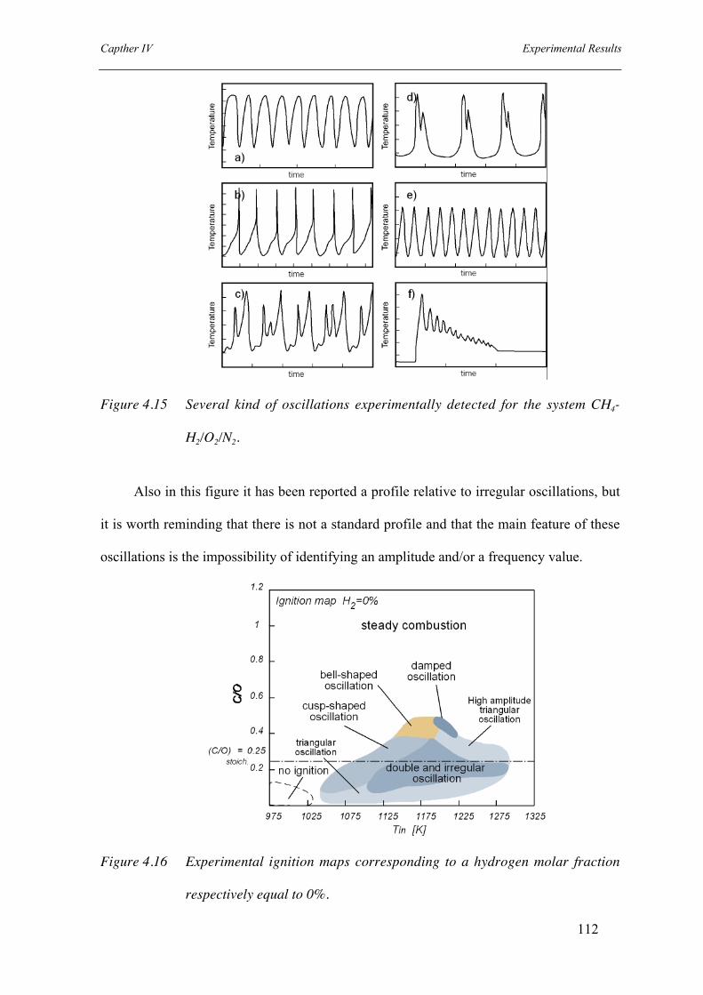
Capther IV Experimental Results
112
Figure 4.15 Several kind of oscillations experimentally detected for the system CH4-
H2/O2/N2.
Also in this figure it has been reported a profile relative to irregular oscillations, but
it is worth reminding that there is not a standard profile and that the main feature of these
oscillations is the impossibility of identifying an amplitude and/or a frequency value.
Figure 4.16 Experimental ignition maps corresponding to a hydrogen molar fraction
respectively equal to 0%.
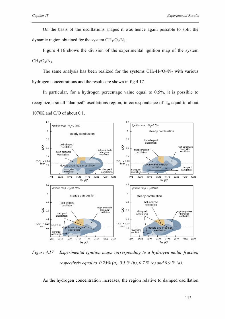
Capther IV Experimental Results
113
On the basis of the oscillations shapes it was hence again possible to split the
dynamic region obtained for the system CH4/O2/N2.
Figure 4.16 shows the division of the experimental ignition map of the system
CH4/O2/N2.
The same analysis has been realized for the systems CH4-H2/O2/N2 with various
hydrogen concentrations and the results are shown in fig.4.17.
In particular, for a hydrogen percentage value equal to 0.5%, it is possible to
recognize a small “damped” oscillations region, in correspondence of Tin equal to about
1070K and C/O of about 0.1.
Figure 4.17 Experimental ignition maps corresponding to a hydrogen molar fraction
respectively equal to 0.25% (a), 0.5 % (b), 0.7 % (c) and 0.9 % (d).
As the hydrogen concentration increases, the region relative to damped oscillation

Capther IV Experimental Results
114
extends and for a hydrogen molar fraction percentage equal to 0.9% it interests a Tin range
comprised between 1050 and 1150K and a C/O range going from values very close to zero
to 0.2.
The same effect concerns the “double and irregular” oscillations zone that becomes
wider as the hydrogen inlet percentage increases. In absence of hydrogen it is possible to
find this oscillations typology in the Tin range of 1100K-1270K and in the C/O range of
0.1-0.4. In presence of hydrogen the whole dynamic behavior zone reduces itself, but the
relative importance of the “double and irregular” oscillations increases. As matter of fact,
for H2 equal to 0.25%, this region extends from Tin equal to 1050 to1250K and C/O range
from 0.15 to 0.35 while for the mixture containing 0.9% of hydrogen. Tin goes from 1050
to1200K and C/O goes from 0.05 to 0.4.
Furthermore, cusp-shaped oscillations disappear from a H2 value of 0.75%, and the
triangular oscillations region becomes evidently smaller.
Bifurcation diagrams
In order to extensively describe the phenomenology detected in diluted oxidation of
mixture of hydrogen and methane it is useful to analyze reactor temperatures in different
conditions. To this aim experimental bifurcation diagrams obtained by fixing one of the
continuation parameters considered above were represented in Figure 4.17, where reactor
temperatures (TR1) measured for C/O ratios of 1, 0.7, 0.4 and 0.1 were reported as function
of Tin.
For C/O=1 the reactor temperature is very close to the isothermal line until an inlet
temperature equal to 1025K. After this value the system evolves trough a dynamic regime,
as the dashed lines show. The maximum working temperature is reached for an inlet
temperature equal to 1050K, but increasing the value of the continuous parameter the mean
reactor temperature decreases and the system reaches a steady solution for Tin. equal to

Capther IV Experimental Results
115
1200K. Then the temperature increment (ΔT) remains almost constant and it is of about
20K. In the previous experimental analysis, realized on the same system with the same
operative conditions, this value was of about 50K. As explained above, it is due to the high
sensitivity of the system to the working parameters but it is anyway worth noting that the
main features of the bifurcation diagrams remain.
Figure 4.17 Bifurcation diagram for the system CH4-H2/O2/N2 for an hydrogen global
percentage equal to 0%.
In figure 4.17 the bifurcation diagram for the system CH4/O2/N2 is reported on
curves parametric in the C/O feed ratio.
For C/O=0.4, hence in reach conditions, for very low inlet temperatures, relatively to
the temperature range analyzed, the temperature increment is very low but then it increases
until the system, for Tin.=1125K, starts oscillating. The temperature increment firstly
increases, reaches a maximum but then it decreases and the system gains a steady
combustion regime for Tin.>1125K.
However the difference between the reactor temperature and the inlet one is of about
20K and this ΔT remains constant in the whole remaining part of the temperatures

Capther IV Experimental Results
116
analyzed.
For C/O=0.7 the system encounter just steady combustion regimes, but also here the
temperature increase increases reaches a maximum and then drops towards the isothermal
line.
This behavior has already been detected in the previous experiments on the same
system and it was named “temperature drop”.
In figure 4.18 it is shown the bifurcation diagram relative to a system CH4-H2/O2/N2
with an hydrogen percentage equal to 0.25%.
For C/O=0.1 the working temperature is relatively close to the isothermal line for
very low inlet temperatures, in fact the temperature increment is of about 20K, then
increasing the continuous parameter the system starts oscillating and the temperature
increment is relatively small. From Tin. of about 1185 K the system evolves trough a stable
regime but the temperature increment is of about 15K.
Figure 4.18 Bifurcation diagram for the system CH4-H2/O2/N2 for an hydrogen global
percentage equal to 0.25%.
For C/O=0.4 the reactor temperature increases as much the inlet temperature is

Capther IV Experimental Results
117
increased, but it starts oscillating for an inlet temperature equal to 1100K. The amplitude of
oscillations decreases increasing the inlet temperature but the average temperature
decreases. In this case the system reaches the highest working temperatures. For
Tin.=1225K the reactor temperature is just 15K higher than the inlet one. Increasing the
inlet temperature the systems does not experiments higher temperature but the temperature
increment becomes nearly constant.
It is evident that increasing the C/O feed ratio the inlet temperature range for which
the dynamic region is established becomes smaller.
For C/O=0.7 the reactor temperature increase increasing the inlet temperature, then it
reaches a maximum. Afterwards it decreases and for values of the continuous parameter
higher than 1225K it becomes just 50K higher than the inlet temperature.
Figure 4.19 Bifurcation diagram for the system CH4-H2/O2/N2 for an hydrogen global
percentage equal to 0.5%.
The same considerations apply to the case C/O=1. In this case the working
temperatures are very close to the temperatures of the system with a C/O feed ratio equal to

Capther IV Experimental Results
118
0.7 but for tin higher than 1050K they become lower. Again the temperature, after a
maximum value, drops towards the isothermal line. This behavior has already been
recognized in the experimental tests realized on the methane oxidation in Mild combustion
conditions.
Figure 4.19 shows the bifurcation diagram for an inlet hydrogen concentration equal
to 0.5%.
The reactor temperature has been plotted as function of the inlet temperature on
curves parametric in the C/O feed ratio. The C/O feed ratios analyzed are again 1, 0.7, 0.4
and 0.1.For C/O=0.1 and inlet temperature lower than 1025K the system evolves trough a
steady combustion. The temperature increment is of about 20K. Then the system starts
oscillating and the temperature amplitude is very small. For Tin. higher than 1150K the
system evolves trough a steady combustion but the difference between the working and
inlet temperature (ΔT) is again 11K.
Figure 4.20 Bifurcation diagram for the system CH4-H2/O2/N2 for an hydrogen global
percentage equal to 0.75%.
For C/O=0.4 the system evolves trough a steady regime and the reactor temperature

Capther IV Experimental Results
119
increases by increasing the inlet temperature until about 1050K. For inlet temperature
comprised between 1050K and 1200K, the system goes trough a dynamic regime. For
Tin.>1200K the temperature increment is very small, it is about 15K.
Increasing the C/O feed ratio up to 0.7, it is possible to see that the system does not
evolves trough oscillating conditions, and the inlet temperature increases increasing Tin ,
reaches a maximum and then it drops towards the isothermal line.
The same considerations apply for the systems with an hydrogen percentage equal to
7.5% and 0.9% respectively reported in figure 4.20 and 4.21.
Figure 4.21 Bifurcation diagram for the system CH4-H2/O2/N2 for an hydrogen global
percentage equal to 0.9%.
Effect of the nature of Diluent: Steam Water
The behavior of the system CH4/O2/N2 in Jet Stirred Flow Reactor (JSFR) has been
studied as function of the main parameters such as the residence time, the dilution degree,
the mixture composition and temperature.
In the previous studies the system has been diluted with nitrogen since the necessity

Capther IV Experimental Results
120
to work with an inert species. In such a way, the oxidation of methane, under non-standard
conditions (high inlet temperature and the high dilution degree), has been studied in
absence of species that could have altered the evolution of the oxidation process. This
study has pointed out that under Mild conditions the CH4/O2/N2 system can give rise to a
dynamic behaviors that have been widely discussed in the previous paragraphs. Such new
phenomenology should be avoided in a combustion chamber since oscillations can be
responsible of mechanical damage to turbines and can lower the efficiency of combustion
process.
With this aim it is interesting to value the effect of the diluent on the dynamic
behavior experimentally detected.
From a practical point of view there are many species that could be used as diluent,
for instance, steam water and carbon dioxide. Their importance comes from the possibility
of recycling the exhausted gases from a combustion chamber in order to pre-heat and dilute
the reactants in a system working in Mild conditions. The exhausted gases are mainly
composed by steam water and CO2. Hence effectively in a real plant they represent the
diluent species.
Steam water and carbon dioxide can have a thermal effect and a chemical effect on
the evolution of the methane oxidation process. The thermal effect is due to the different
heat capacities whereas the chemical effect is due to the possible breakdown of these two
species that would result in an enhancement of radical species.
Hence in this paragraph the oxidation process of system CH4/O2 under Mild
condition has been characterized as function of the nature of the diluent. In particular the
system has been diluted with nitrogen and steam water.

Capther IV Experimental Results
121
Experimental Ignition Map
The effect of the nature of the diluent has been experimentally tested in the Jet
Stirred Flow Reactor described in the chapter III.
The working parameters are resumed in the tab 4.22. The residence time is 0.5 sec,
the temperature range is comprised between 1000K and 1250K, the C/O feed ratio has
been changed from value very close to zero up to 1.2. In these experimental tests nitrogen
and steam water dilute the system up to 90%. In particular steam water has been added in
percentage equal to 10% and 20% of the overall dilution degree.
Reactor JSFR
Residence Time 0.5 sec
Feed Ratio (C/O) 0.05-1.2
Dilution degree
Steam water
90%
10%-20%
Pressure 1.17 atm
Temperature 1000 K-1250 K
Tab. 4.22 Chosen working conditions for Mild Combustion studiesin systems diluted
with steam water.
The experimental study performed on methane Mild oxidation has focused on the
identification of the system behavior as function of the inlet temperature (Tin.), C/O ratio
and dilution levels. During the set of experiments, the temporal temperature profiles,
recorded by means of a facility well described in chapter III, suggested that the oxidation
of methane in conditions typical of Mild processes, gives rise to a complex dynamic
behavior and the attention has been focused mainly on the characterization of this new
phenomenology.

Capther IV Experimental Results
122
The first approach to this problem was the partition of the working conditions for
which the system evolves through stable combustion or oscillating regimes.
Since the residence time τ, the pressure and the dilution level have been fixed, the
only parameters to set up are the inlet temperature and the carbon-oxygen feed ratio C/O.
In order to have a descriptive indication on possible stable or periodic states, the results
were resumed in bifurcation maps of the system by using Tin. and C/O ratio as continuation
parameters for the two dilution levels considered. Any point of the Tin.-C/O plane
represents an inlet condition, and it has been classified on the basis of the system stability.
The systems that have been analyzed are CH4/O2/N2, CH4/O2/N2-H2O(10%) and
CH4/O2/N2-H2O(20%).
Figure 4.23 Tinlet-C/O bifurcation map obtained for a dilution level of 90%, τ=0.5 sec for
the system CH4/O2/N2.
The experimental tests for the system CH4/O2/N2 have been repeated in order to
confirm the first results and also to properly compare the results obtained for the other two

Capther IV Experimental Results
123
systems. In fact the system is very sensitive to uncontrollable parameters, such as the
environmental temperature, that can affect the process in terms of heat exchange, and
slightly change the evolution of the oxidation.
Figure 4.24 Bifurcation diagrams for several C/O feed ratios for the system CH4/O2/N2.
The experimental bifurcation map obtained for the system CH4/O2/N2 is reported in
Figure 4.23. The main features of the dynamic behavior have been found out again even if
the extension of the dynamic region is slightly different in comparison with the maps
obtained in the other experimental tests. Anyway these slight changes in the extension of
the dynamic region were expected.

Capther IV Experimental Results
124
The ignition map shows that the widest region corresponds to stable combustion
where a single step ignition leads the system to a steady working temperature.
The steady combustion is the only phenomenology occurring in the region of richest
C/O ratios down to 0.6 in the whole temperature range analyzed. At lower C/O ratios and
Tin higher than 1040 K a region where dynamic behavior occurs is also recognized. For
C/O=0.6 temperature oscillations occur in a range of 50K, from Tin. = 1150K up to 1200K.
The oscillating temperature region enlarges by decreasing the C/O ratio thus covering the
temperature range between 1040K up to 1250 K in correspondence of the leanest C/O
ratios.
Furthermore the same oscillation typologies, defined in the first experimental tests,
have been recognized. In this case the temperature profiles are not reported since the
attention has been focused on the effect of steam dilution on the extension of the dynamic
region.
Figure 4.24 reports the temperature of the reactor (Treactor) as function of the inlet
temperatures (Tin) for several rich mixtures, respectively characterized by a C/O feed ratio
equal to 0.7, 0.8,1. For all these mixtures it is possible to recognize the same trend of the
Treactor as function of Tin.
The working temperature is close to the isothermal line (dashed line) for low values
of the Tin in the analyzed temperature range. As the inlet temperature is increased Treactor
slowly increases, reaches a maximum and then decreases towards the isothermal line.
The results for the systems CH4/O2/N2-H2O(10%) and CH4/O2/N2-H2O(20%) have
been resumed in ignition maps following the same methodical approach used for the
system CH4/O2/N2.
Figure 4.25 shows the ignition maps for the former system. Also in this case it is
possible to see that for the most of the analyzed inlet conditions the system evolves trough

Capther IV Experimental Results
125
a steady combustion. In fact for rich mixtures, characterized by a C/O feed ratio higher
than 0.6, temperature profiles show an sudden jump of reactor temperature that then goes
down to the steady value. For temperature higher than 1040K and C/O feed ratio lower
than 0.6 it is possible to identify oscillations.
Figure 4.25 Tinlet-C/O bifurcation map obtained for a dilution level of 90%, τ=0.5 sec for
the system CH4/O2/N2-H2O(10%)
For C/O=0.6 the dynamic behavior has been detected in a relatively small
temperature range that goes from 1150 K to 1180K. Then for C/O=0.4 the temperature
range enlarges and goes from 1120K to the highest exploited temperature values (1250K).
Decreasing the C/O feed ratio the region enlarges and cover almost all the temperature
range considered for the experiments. For very lean mixtures (C/O < 0.05), only stable
combustion is detectable.
Also for the system CH4/O2/N2-H2O(10%) the reactor temperature has been plotted
versus the inlet temperature for several C/O feed ratio. The bifurcation diagrams are

Capther IV Experimental Results
126
reported in figure 4.26. It is possible to recognize the same trend discussed for the system
CH4/O2/N2.
As the inlet temperature increases the Treactor increases, reaches a maximum, and the
goes towards the isothermal line. This behavior has been named “temperature drop” and
will be discussed in Chapter V. In this case it is also possible to see that, for very high
values of the inlet temperature, the difference between the Treactor and Tin is relatively small
and almost constant. Such value is equal to about 30K.
Figure 4.26 Bifurcation diagrams for several C/O feed ratios for the system CH4/O2/N2-
H2O(10%).

Capther IV Experimental Results
127
For the system CH4/O2/N2-H2O(20%) the ignition map is reported in figure 4.27.
Also in this case for mixtures characterized by a C/O feed ratio higher than 0.6 in the
whole analyzed temperature range methane oxidation occurs in steady conditions. For C/O
lower than 0.6 and Tin higher than 1040K experimentally temperature oscillations can be
detected. Once again, the dynamic region interests a small temperature range (1150K-
1180K) for values of the parameter C/O comprised between 0.4 and 0.6. For lower C/O
range the dynamic region enlarges and interests almost the whole temperature range
considered during the experimental tests.
Figure 4.27 Tinlet-C/O bifurcation map obtained for a dilution level of 90%, τ=0.5 sec for
the system CH4/O2/N2-H2O(20%).
The bifurcations diagrams are reported in figure 4.28. Reactor temperature is plotted
as function of the Tin in for several C/O feed ratios. The same trend, described before for
the system with a lower steam water percentage, is here recognizable.
For Tin=1225K and Tin=1250K, the difference between the Treactor and Tin (ΔT)

Capther IV Experimental Results
128
becomes relatively small and the ΔT reaches a constant value for any analyzed C/O
considered in the paragraph.
Figure 4.28 Tinlet-C/O bifurcation map obtained for a dilution level of 90%, τ=0.5 sec for
the system CH4/O2/N2-H2O(20%).
Simplified configuration for fluid-dynamic tests
After the design of the tubular reactor, the attention has been focused on the mixing
devise. As discussed in chapter III, the configuration chosen to mix reactants forecasts fuel
is injected in the main duct trough nozzles disposed on the perimeter of a duct cross

Capther IV Experimental Results
129
section.
The efficiency of the mixing section has been evaluated by means of experimental
characterization of fluid-dynamic behavior of a simplified facility working at ambient
temperature.
Obviously the geometry of this facility is very similar to the plug flow reactor
designed for the study of the oxidation process in Mild Condition. The system is shown in
fig. 4.29.
Figure 4 .29 Simplified configuration for fluid-dynamic tests.
The facility presents an inlet part, a quartz tube and an outlet part. The first part
consists in a flanged tube that is joint to the mixing section by means of bolts. The main
flow is fed from the bottom of the first part of the facility while the lateral flow is injected
from round, equally spaced tubes displaced on the perimeter of the first section at the end
of the first section. The inlet section has an inner diameter equal to 1.4 cm. A convergent
allows reducing this dimension to 1 cm to join the mixing section to the quartz tube. The
convergent has a linear geometry and its slope is 26°. The mixing section is displaced at an
axial distance equal to the diameter of the duct to the convergent. The mixing device has

Capther IV Experimental Results
130
10 tubes with a inner diameter equal to 0.05 mm. The inner dimension of tubes can be
changed in order to perform the study of the mixing efficiency as function of the
dimension of holes. The geometry of the mixing part slightly differs from the real reactor
mixing device configuration since the latter one will have 6 holes with an inner diameter
equal to 0.80mm. The simplified facility has been built before the numerical studies on the
mixing efficiency, hence it has been built taking into account just the literature suggestions
(Holdeman et al. 1996). Two distributors insure an equal division of the lateral flows
among the 10 tubes. Each of the two distributors feeds 5 tubes.
The main flow mix with the lateral jest and enters the quartz tube. Quartz allows
having a facility optically accessible. Furthermore the outlet part is provided of a quartz
window in order to perform optical diagnostic analysis. Anyway this discussion is
remanded to next section.
The last part of the facility is provided of four outlets in order split the main flow in
four flows and have a low velocity. In this way the pressure in the system will be
atmospheric. As matter of fact the flow rates used in the system are very high. Hence there
is the necessity of avoiding to work in sonic condition, which would lead to an increase in
pressure.
In this facility fluorescence measurements will be performed to test the efficiency of
the mixing device. In particular acetone is used as a tracer in a helium flow and it is fed
from the lateral injectors inside the mixing section where it blend with air.
The use of acetone has widely conditioned the choice of materials. In fact the facility
has been realized in Teflon, while rigid tubes are in stainless steel and flexible tubes, such
as the ones that link the distributors to injectors, are in Teflon.
Fluorescence measurements
In order to test the reactor configuration from the fluid-dynamic point of view the

Capther IV Experimental Results
131
model of the alumina reactor, able to work at ambient temperature has been used. An
optical diagnostic system for fluorescence measurements in different sections of reactor
has been set up. In particular, the second harmonic of a Nd:YAG laser (λexc=266 nm) has
been used in order to excite the acetone injected as tracer along with helium in the lateral
jets in order to study the their mixing degree with the main flow.
Figure 4.30 Experimental set-up for fluorescence measurements
The optical diagnostic used was a bi-dimensional implementation of a simple 90°
LIF collection scheme. To this aim the laser beam was shaped as a thin (200 µm) sheet by
using a cylindrical telescope. The laser sheet (0.7 cm tall) crosses the reactor at the chosen
section. The scattered light was filtered by means of a band-pass filter (350-450 nm). The
resulting image is collected by means of an ICCD camera sensitive in this spectral range.
For each test run 200 images were collected in the same experimental condition and added
in order to smooth away laser pulses energy oscillation and to increase the signal-to-noise
ratio of measured spectra.
Acetone is often used as tracer in combustion device in order to study the species
distribution in the reaction zones. The electronic transition that characterizes spectra of
carbonyl compounds is generally known as n→ π* . It is due to one of the two
non-bonding electrons of the oxygen atom, which is excited in the antibonding orbital (π*)

Capther IV Experimental Results
132
of C=O group. This transition characterizes each carbonyl compound independently on the
molecule to which the carbonyl group belongs. The nature of the atoms bonded with >C=O
group can partially modify the spectrum of n→ π* . Generally this results in the
appearance of additional spectral structures, observable along with the one typical of
n→ π* .
Figure 4.31 Spectroscopic behavior of carbonyl compounds.
The luminous signal related to this electronic transition has been summarized for
different ketones in Figure 4.31a, b and c (de Joannon et al, 2001). In Fig. 4.31a the
absorption spectrum of a water solution of acetone has been reported as representative of
absorption characteristics of aliphatic ketones. It covers the wavelength region between
210 and 310 nm with a maximum at about 270 nm. Similar behavior has been reported in
literature (Hansen and Lee, 1975/2) for heavier ketones too.

Capther IV Experimental Results
133
The fluorescence spectrum characteristic of n→ π* transition generally covers a
wavelength region between 350 and 550 nm with a maximum at about 420 nm, such as
shown by the fluorescence spectra relative to acetone and pentanone (Hansen and Lee,
1975/2) reproduced in Figure 4.31b. This behavior has been confirmed by the spectrum
collected in the present work from a water solution of acetone, reported in Figure 4.31c.
The experiments aim to understand the dependence of the mixing degree on the
parameter jet to stream mass-flow ratio J (J= ρj vj2/ρs vs2). The system is composed by air
and helium. Helium gurgles in a bath of acetone and the outlet mass flow rate is composed
by helium and acetone that enter the main duct from the lateral injections and mix with the
main flow.
This noble gas has been chosen as lateral flow since we have tried to reproduce the
same values of J there would be the in the real system while keeping equal the velocities.
This constraint comes from the same system the density of the main flow is very low since
the high inlet temperatures. On the contrary the simplified facility works at environmental
temperatures hence the ratio between the densities of the main and the lateral flow rate is
much higher from the one of the real configuration. To reduce this difference the molecular
weight of the injected flow has been chosen as small as possible since the choice of the air
as main flow is due to economical reasons.
Anyway in the first set of measurements the experiments have been realized
changing the helium volumetric flow rate, hence its velocity, while keeping constant the air
volumetric flow rate.
Two-dimensional fluorescence images of the half section of the reactor collected at
1mm, 10mm and 20mm from the mixer exit for different J have been collected and
discussed.

Capther IV Experimental Results
134
Experimental tests realized in the simplified configuration forthe study of the fluid-dynamic
The aim of the experiments is to understand the dependence of the mixing degree on
the parameters typical of the jet in cross flow configuration such as the momentum of the
jet to maim stream ratio J, the number (n) and the dimension of holes.
The system is composed by air and helium. Helium gurgles in a bath of acetone and
the outlet mass flow rate is composed by helium and acetone that enter the main duct from
the lateral injections and mix with the main flow.
This noble gas has been chosen as lateral flow since we have tried to reproduce the
same values of J there would be the in the real system while keeping equal the velocities.
This constraint comes from the same system the density of the main flow is very low since
the high inlet temperatures. On the contrary the simplified facility works at environmental
temperatures hence the ratio between the densities of the main and the lateral flow rate is
much higher from the one of the real configuration. To reduce this difference the molecular
weight of the injected flow has been chosen as small as possible since the choice of the air
as main flow is due to economical reasons.
In figure 4.30 it is represented a two-dimensional sketch of the simplified
configuration that has been used in order to characterize the mixing of this geometry.
The sketch shows the first section with an inner diameter equal to 14mm, than the
linear convergent with a slope of 26°, and then the third section with a inner diameter of
10mm. In particular this sketch shows 6 injectors equally spaced along the perimeter of the
first section at an axial distance from the convergent equal to 7mm.
For all the configurations that have been analyzed in this chapter the origin of the
system is located at the end of the convergent on the axis of the cylindrical duct. Hence the
injection plane is at an axial coordinate equal to x=-11mm.

Capther IV Experimental Results
135
The geometric parameters that have been investigated are: the number of holes (n),
the diameter of holes (d), the protrusion of the injectors inside the duct (p).
For any analysis the range of the value J is sufficiently wide in order to analyze the
mixing in a under-penetration and over-penetration conditions. The value of J is changed
varying the helium flow rate. The main flow rate is fixed to 25000 Nl/h, in such a way to
have a velocity in the first section equal to 45 m/s, while the lateral flow rate, composed by
helium and acetone, changes from 600Nl/h to 3900Nl/h.
Figure 4.30 Sketch of the simplified configuration for the fluid-dynamic study.
The amount of the acetone in the helium flow may change as function of the
experimental condition. Some calculations have been performed in order to estimate the
concentration of acetone in the reactor once it is mixed with the main flow. Fig.4.31 shows
the volumetric acetone concentration as function of the helium flow rate. It changes from
6x10⁻⁶ a 1x10⁻⁵ but it seems to be almost constant from a helium flow rate higher than 1000
Nl/h.
The results are important for the analyses of the fluorescence measurements that
have been realized on the simplified configuration for the study of the mixing degree.
For any considered geometry, it has been calculated the Standard Deviation of the
fluorescence intensity profiles along a diameter of the duct. This statistic tool gives an
indication on the uniformity of fluorescence signal along the reactor diameter.

Capther IV Experimental Results
136
The lower the StD is, the more uniform the acetone concentration is. Hereafter the
standard deviation StD or mixing dis-uniformity are used with the equivalent meaning. The
StD has been calculated as function of the parameter J at three axial distance from the
convergent respectively equal to 1mm, 1cm e 2cm.
Figure 4.31 Acetone volumetric concentration inside the third section of the simplified
set-up as function of the helium flow rate (Nl/h).
The standard deviation is calculated by means this formula:
N
xxStD
N
ii∑
=
−= 1
2)(
where
�
xi is the normalized pixel intensity,
�
x the mean of data and N the
number of pixels of the fluorescence profile.
The literature (Holdeman, 1992) suggests that for values of the StD lower than 0.1
the system has reached a very good mixing and that for StD lower than 0.2 the mixing can
be considered acceptable.
In this section it has just be presented the experimental measurements relative to the
system with 10 injectors located on the wall of the cylindrical duct. Hence the images

Capther IV Experimental Results
137
collected during the experimental tests, the radial profile of the fluorescence intensity and
the standard deviation analyses has been reported in order to show the approach to the
study of the mixing in the jet in cross-flow configuration. In the other considered cases it is
just reported the standard deviation analysis of the fluorescence intensity. All the images
and intensity profiles relative to these other cases are reported in the appendix.
10 injectors located on the wall of the cylindrical duct
The first analyzed geometry presents 10 injectors with an inner diameter equal to 0.5
mm. They are equally displaced on the perimeter of the cylindrical duct at 36° of distance
from each other.
In this case the optimal value of the momentum of the jet to mainstream ratio J
according to Holdeman equations is equal to 32 (JHopt.). The numerical simulations have
been run for a wide range of J, from 2 to 64, in such a way it has been possible to
analyzing the mixing in a wide range of conditions. If fact the analyses have been
performed for J values lower and higher than the JHopt..
The bi-dimensional implementation of the fluorescence measurements realized for
this configuration is presented in figure 4.32. The acetone distribution and concentration
inside the reactor is represented by the fluorescence intensity of pixels of images collected
by means of the optical facility for the fluorescence measurements. In figure 4.32,
fluorescence intensity is represented by means of a linear false color scale reported in the
figure. The scale has been subdivided into sixteen different levels, hence colors, and the
pixel intensity goes from zero to 1800. The white color corresponds to fluorescence
intensity equal to zero; hence it indicates the complete absence of acetone. The
fluorescence intensity has been normalized respect to the highest intensity value of all the
images collected for the several configurations considered, in order to compare all the
experimental results among them.

Capther IV Experimental Results
138
The images have been collected for three different cross sections located in the plane
x=0 and at an axial distance equal to x=1mm, x=1cm and x=2cm. In the figure it is also
reported the laser beam that hits the cylindrical duct.
The figure allows the analysis of the acetone distribution as function of the parameter
J, once the axial position has been fixed, as well as the analysis of the acetone distribution
as function of the axial position if the value of the parameter J has been fixed.
At an axial position x=1mm, for any J value there is a internal zone where there is
not any fluorescence intensity signal. This region tends to diminish as the parameter J
increases. For J>40 it almost disappears but in any analyzed case, the acetone tends to
accumulate in the near-wall region.
At an axial distance fro the convergent equal to 1 cm the fluorescence intensity
signal present the same trend as function of the parameter J.
For J=2 and J=6 there is an internal region with no acetone, but for J=8 a small
concentration of acetone is detectable also in this region, even if the fluorescence intensity
is very low.

Capther IV Experimental Results
139
Figure 4.32 Fluorescence Intensity images as function of the parameter J in curves
parametric on the axial position for the configuration with 10 holes
Capther IV Experimental Results
140
positioned on the wall of the cylindrical duct.
From J=12 the central zone is invested increasingly more by acetone until J=64,
when the acetone cover almost completely and uniformly the whole section except for a
low internal core.
For the last considered axial position, it is possible to note that the internal core with
no acetone persists from J=2 to J=4, but for J=6 the acetone spread out on all the cross
section even if the distribution is not uniform.
The fluorescence signal becomes increasingly more uniform and from J=50 to J=64
the signal suggests that the jet in cross flow configuration ensures a good mixing of the
tracer.The other way to analyze the images is to consider the fluorescence intensity as
function of the axial position for a fixed J value.
In general the mixing uniformity improves with the axial position. For J=2 and J=4,
at x=1mm the intensity signal is detected just in the near-wall region. For x=1cm and x=2
cm the situation does not improve so much but the central region with no acetone
diminishes significantly. The same considerations apply for J=6 but in this case for x=2cm
the acetone is present with a relative low concentration also in the center of the cross
section. The same situation is proposed again for the sequence of images collected for J=17
but at x=2cm the acetone spreads on the whole area with a significant acetone
concentration in the center of the section.
For J=32 also at x=1cm the distribution of acetone begins to be significant in the
center region.
For J=50 and J=64 and an axial distance equal to 1mm the internal segregated area is
very narrow. It diminishes at x=1cm and it completely disappears at x=2cm and this
indicates a very good mixing.
In fig.4.33 the fluorescence intensity signal is plotted along a diameter of the duct at

Capther IV Experimental Results
141
the known axial distances for any J value analyzed.
Figure 4.33 Fluorescence Intensity signal profiles as function of the parameter J in
curves parametric on the axial position for the configuration with 10 holes
positioned on the wall of the cylindrical duct.

Capther IV Experimental Results
142
In these figures the fluorescence intensity has been normalized respect to its mean
value for each condition. In such a way the profiles have been made independent on the
acetone concentration and they can be reasonably compared among them.
The same analyses and considerations can be realized taking into account the
normalized fluorescence profiles reported in figure 4.33. In this case the uniformity of
acetone distribution is reached when profiles becomes flat.
For J=2 the profiles indicate that the tracer accumulates in the lateral area and that
there is no acetone for a wide portion of the diameter. In this case the jets under-penetrate
inside the main duct and the acetone remains segregated in the near-wall region. J
represents the best condition when it is equal to 64 where the profiles are sufficiently flat
for all the axial positions.
In fig.4.34 the non-uniformity of the mixing, calculated on the basis of the standard
deviation, is presented as function of the parameter J on curves parametric on the axial
position. The StD has been calculated considering the normalized pixel fluorescence
intensity values presented in fig. 4.33.
The higher the momentum of the jet to mainstream ratio, the lower the StD is for any
axial distance. As matter of fact, the StD decreases monotonically and slowly as the
parameter J is increased. At x=1mm the StD goes from 1.3 to 0.25, while for x=1cm it goes
from values very close to 1 to 0.11, and for x=2cm it interests J values from 0.6 to 0.06.
The best uniformity of mixing is reached at x=1cm and x=2cm for values of J
respectively equal to 64 and 50. The StD becomes lower than 0.2 for J=50 at x=1cm and
for J=23 at x=2cm. For x=1mm the lowest StD value is reached for J=64 but it is equal to
0.28.
Therefore it is possible to state that at x=1mm the discussed configuration does not
provide for a good distribution of the acetone. Furthermore it is needed a very high value

Capther IV Experimental Results
143
of the parameter J to have a good mixing of the tracer.
Figure 4.34 Standard Deviation of the fluorescence intensity signal along a diameter of
the duct as function of the parameter J on curves parametric in the axial
position.
6 injectors with d=0.9 mm located on the wall of the cylindrical duct
In fig.4.35 the non-uniformity of the mixing, calculated on the basis of the standard
deviation, is presented as function of the parameter J on curves parametric on the axial
position for the system with 6 injectors with d=0.9 mm located on the wall of the
cylindrical duct The StD has been calculated considering the normalized pixel fluorescence
intensity values reported in appendix for this case.
The higher the momentum of the jet to mainstream ratio, the lower the StD is for any
axial distance. As matter of fact, the StD decreases monotonically as the parameter J is
increased. For x=2cm it mainly diminishes from J=0.5 to J=6, than for all the axial
distances it seems to reach a constant value. At x=1mm the StD goes from 0.9 to 0.21,
while for x=1cm it goes from values very close to 78 to 0.16, and for x=2cm it interests J
values from 0.68 to 0.14.
The StD is never lower than 0.1 but for x=2cm is lower than 0.2 for J>6. For x=1cm
it is lower than 0.2 for J>14 while at x=1mm it always higher than this value.

Capther IV Experimental Results
144
Figure 4.35 Standard Deviation of the fluorescence intensity signal along a diameter of
the duct as function of the parameter J on curves parametric in the axial
position.
6 injectors with d=0.8 mm located on the wall of the cylindrical duct
In fig. 4.36 the non-uniformity of mixing is plotted as function of the J value at the
three axial distance x=1mm, x=1cm and x=2cm. The standard deviation is calculated on
the basis of the normalized fluorescence profile reported in figure 5.3.8.
Figure 4.36 Standard Deviation of the fluorescence intensity signal along a diameter of
the duct as function of the parameter J on curves parametric in the axial
position.
For x=1cm the StD becomes lower than 0.2 for J=16, while for x=2cm for J=7. For

Capther IV Experimental Results
145
this axial distance it reaches the minimum value for J=11 and than it is constant for higher
value of J.
For x=1mm the lowest value is 0.26 and it competes to the highest value of J here
analyzed.
6 injectors with d=0.9 mm protruded 1mm inside the cylindrical duct
In figure 4.37 the Standard Deviation of the fluorescence intensity signal along a
diameter of the duct as function of the parameter J on curves parametric in the axial
position are reported for the system with 6 injectors with d=0.9 mm protruded 1mm inside
the cylindrical duct
Figure 4.37 Standard Deviation of the fluorescence intensity signal along a diameter of
the duct as function of the parameter J on curves parametric in the axial
position.
In the case of x=1mm, the Standard deviation decreases monotonically but in at
x=1cm and x=2cm it presents a minimum value respectively for J=6 and J=3. As matter of
fact, the non-uniformity of the mixing increases after these values increase and the StD is
lower than 0.2 just for J=3.
6 injectors with d=0.8 mm protruded 1mm inside the cylindrical duct
In fig.4.38 it is shown the non-uniformity, hence the standard deviation of the
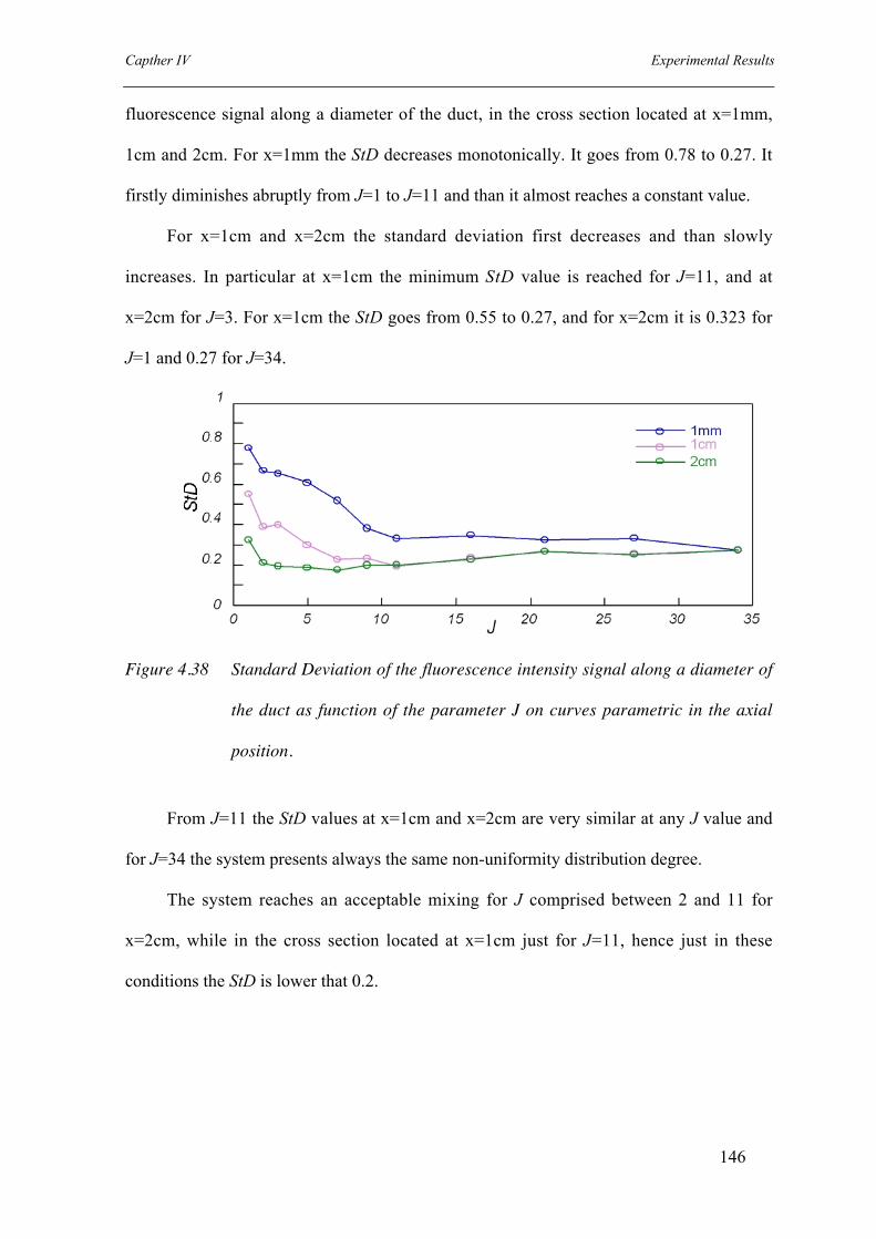
Capther IV Experimental Results
146
fluorescence signal along a diameter of the duct, in the cross section located at x=1mm,
1cm and 2cm. For x=1mm the StD decreases monotonically. It goes from 0.78 to 0.27. It
firstly diminishes abruptly from J=1 to J=11 and than it almost reaches a constant value.
For x=1cm and x=2cm the standard deviation first decreases and than slowly
increases. In particular at x=1cm the minimum StD value is reached for J=11, and at
x=2cm for J=3. For x=1cm the StD goes from 0.55 to 0.27, and for x=2cm it is 0.323 for
J=1 and 0.27 for J=34.
Figure 4.38 Standard Deviation of the fluorescence intensity signal along a diameter of
the duct as function of the parameter J on curves parametric in the axial
position.
From J=11 the StD values at x=1cm and x=2cm are very similar at any J value and
for J=34 the system presents always the same non-uniformity distribution degree.
The system reaches an acceptable mixing for J comprised between 2 and 11 for
x=2cm, while in the cross section located at x=1cm just for J=11, hence just in these
conditions the StD is lower that 0.2.

Capther V Numerical Results
148
Charter V
Numerical Results
Numerical Ignition Maps with the ChemKin Software
The experimental results reported in the previous chapter underlined the existence
of a complex dynamic phenomenology related to the oxidation of the methane in condition
typical of Mild Combustion. The availability of feasible methane oxidation kinetic models
suggested the possibility of studying the dynamical behavior experimentally identified also
by means of a numerical approach. Such a study has a double aim: the former concerns the
possibility of verifying numerically the existence of the dynamic phenomenology found
out during the experiments; the latter is the comprehension of the methane oxidation
kinetic pathways during the oscillating regimes. As described in the chapter III, the
ChemKin package software and its application Aurora have been used to perform this
analysis. Aurora allows simulating the behavior of a perfect stirred flow reactor in transient
conditions.
For a first analysis, two different models were used for simulating the behavior of the
CH4/O2/N2 system in Mild condition in a stirred flow reactor: the model by J. Warnatz and
V. Karbach (1997) and the model by F. Battin-Leclerc and P. Barbe (1997) from the Nancy
research group. Hereafter, they will be respectively named “Warnatz” and “Nancy” model.
The “Warnatz” model is composed by 34 chemical species and 164 reactions, the
other one by 64 chemical species and 439 elementary reactions. The different number of
reactions is due to the higher number of reactions involved in the recombination channel of
the methane kinetic mechanism. In fact the ”Nancy” model simulates the kinetic behavior
of methane until the formation n-butane while the “Warnatz” model until ethane formation.
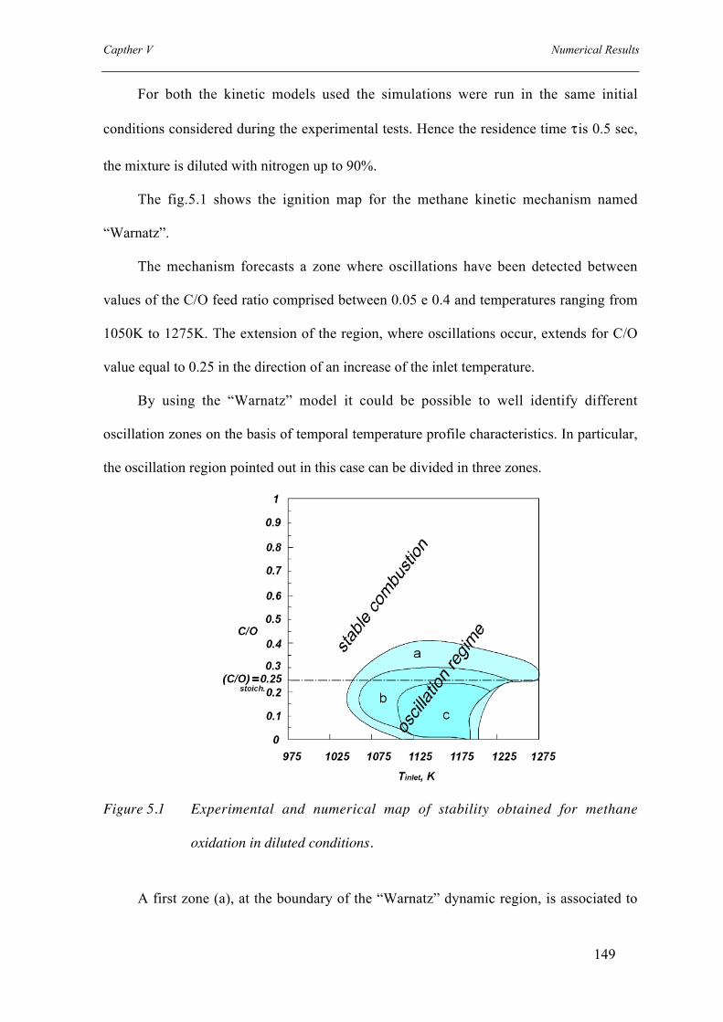
Capther V Numerical Results
149
For both the kinetic models used the simulations were run in the same initial
conditions considered during the experimental tests. Hence the residence time τ is 0.5 sec,
the mixture is diluted with nitrogen up to 90%.
The fig.5.1 shows the ignition map for the methane kinetic mechanism named
“Warnatz”.
The mechanism forecasts a zone where oscillations have been detected between
values of the C/O feed ratio comprised between 0.05 e 0.4 and temperatures ranging from
1050K to 1275K. The extension of the region, where oscillations occur, extends for C/O
value equal to 0.25 in the direction of an increase of the inlet temperature.
By using the “Warnatz” model it could be possible to well identify different
oscillation zones on the basis of temporal temperature profile characteristics. In particular,
the oscillation region pointed out in this case can be divided in three zones.
Figure 5.1 Experimental and numerical map of stability obtained for methane
oxidation in diluted conditions.
A first zone (a), at the boundary of the “Warnatz” dynamic region, is associated to

Capther V Numerical Results
150
dumped oscillations, which seem to appear during the transitions between the stable and
the oscillatory regimes. In the second (b) and the third (c) zones respectively cusp-shape
and triangular-shape oscillations were found.
Fig. 5.2 shows a temporal temperature profile obtained for C/O=0.3 and for an inlet
temperature equal to 1073K. The system evolves trough a dumped periodic oscillation.
Figure 5.2 Dumped oscillation obtained for C/O=0.3 and Tinlet= 1073K.
The region associated to the dumped oscillation in the C/O-Tinlet plane mainly
extends for C/O feed ratios higher than 0.3 and they interest all the temperature range
where oscillations have been numerically detected. Furthermore, this region evidently is a
transition zone since it extends between the stable combustion region and the oscillating
region.
For Tinlet equal to 1073K and C/O= 0.2 the system evolves, using a terminology
applied for the description of the different temperature profiles in the paragraph, trough a
“cusp” oscillation.
This profile is reported in fig.5.3. It underlines an important feature of this kind of
oscillations, in fact they show the same values of frequency but not the same amplitude.

Capther V Numerical Results
151
Figure 5.3 Cusp oscillation obtained for C/O=0.2 and Tinlet= 1073K.
The region where “cusp” oscillations have been numerically identified mainly
extends from C/O feed ratio that range form 0.3 to 0.4 and for temperatures comprised
between 1050K and 1225K, furthermore for C/O comprised between 0.1 and 0.3 and
temperatures between 1048K and 1175K.
Finally the region relative to triangular oscillations extends for C/O values comprised
between 0.05 and 0.25. The figure 6.4 shows the typical temporal profiles relative to
triangular oscillations. It has been detected for C/O=0.2 and T=1173K.
Figure 5.4 Small amplitude triangular oscillations obtained for C/O=0.2 and Tinlet=
1173K.
In the numerical ignition map the region that competes to the dynamic behavior
extends on a narrower area in comparison with the one experimentally detected.
Hence the model is able to reproduce the oscillatory behavior but does not reproduce

Capther V Numerical Results
152
all the kind of oscillations experimentally identified.
Further analyses have been realized using the “Nancy” model. The results have been
resumed in the ignition map reported in fig.5.5. Also this model is able to reproduce the
dynamic behavior experimentally detected. The oscillatory behavior extends from 1025K
to 1275 K and for C/O feed ratios comprised between values very close to zero and 0.4.
Also in this case the extension of the region were oscillations occur is under-
estimated in comparison with the region experimentally detected.
Both the models are able to reproduce “dumped”, “cusp” and “triangular”
oscillations. They can also predict “double” oscillations. They have been detected for
stochiometric fuel-comburent C/O ratio and for very high temperatures. Anyway the region
relative to such oscillations is very narrow and it was not possible to identify a significant
region in the ignition map.
Figure 5.5 Numerical map of stability obtained for methane oxidation in diluted
conditions.
A comparison between the models has not been realized since the aim of the

Capther V Numerical Results
153
numerical analyses was to see whether kinetic models available in literature were able to
reproduce the new phenomenology identified during the experimental tests.
Hence a detailed analysis of the difference between the two models has not been
realized.
Effect of the heat transfer coefficient
Another parameter that can affect the insurgence and the features of the dynamic
behavior is the global heat transfer coefficient. Hence a numerical analysis has been run in
order to assess how much the dynamic region is sensitive to a change of this parameter.
Two coefficients have been considered. They are equal respectively to 4*10-4 cal/cm2 sec
K and 2*10-3 cal/cm2 sec K. The attention was mainly focused on the extension of the
dynamic region as function of the heat coefficient and not on oscillations features. Figure
5.6 shows the ignition maps obtained from the two coefficients.
Figure5.6 Ignition maps obtained as function of the global heat transfer coefficient.
Changing such parameter, the same typologies of oscillations were been found out,

Capther V Numerical Results
154
but they are not reported in the figure. The dynamic regions extends for the same values of
the C/O feed ratios but not for the same range of temperatures. As matter of fact, the
oscillation region relative to the coefficient 4*10-3 cal/cm2 sec extends from 1050K to
1275K, whereas the oscillating region relative to the coefficient 2*10-3 cal/cm2 sec from
1050K to 1200K.
The shape of the two areas is similar and they almost coincide for low values of
temperature and for lean mixtures. For both the two global heat transfer coefficients the
dynamic regions extend for a stochiometric mixture.
Analyses of the frequency
The computed oscillation frequencies were reported in Fig.5.8 as a function of the
inlet temperature on C/O ratio parametric curves.
Figure 5.8 Numerical frequency profile as function of inlet temperature for different
C/O ratios.

Capther V Numerical Results
155
For this analysis the “Warnatz” model has been chosen. It is easily shown that for a
fixed C/O ratio the frequency increases with temperature whereas it decreases with a C/O
increase, thus confirming the general trend obtained by means of the experimental analysis.
However, the numerical computation is not able to predict the absolute values of the
frequencies. In fact, they range from 0.2 Hz to values higher than 30Hz, whereas the
highest experimental frequency value is 7Hz.
Numerical Ignition map with the Dsmoke Software
In the numerical analyses, realized to characterize numerically the behavior of the
system CH4/O2/N2, the model “TOT0310” of the research group of the Chemical
Department of the University of Milan (E.Ranzi et al., 1994) has been used. It counts 250
species involved in more than 5000 reactions and has been extensively validated across a
wide range of conditions (E.Ranzi et al., 1994; E.Ranzi et al., 2001). Hereafter the model
will be referred as “Ranzi” model.
The possibility to predict the dynamic behavior by means a more complex kinetic
model, that maybe could reproduce some features of oscillations not forecasted by the
other two models, has engender interest.
The main pathways of methane combustion can be summarized briefly as follows.
CH4 oxidation undergoes H abstraction with the consequent formation of the methyl
radical. CH3 reacts with O2 to form CH3O whose decomposition produces formaldehyde.
H-abstraction and dehydrogenation of CH2O successively form HCO and CO. Finally, CO
interaction with OH produces CO2. At low temperatures, CH3 can add on O2 forming a
CH3OO radical, whose main fate is CH2O formation or CH3OH, at high pressures. At high
temperatures, OH attacks on CH3 can generate CHi radicals whose interactions with O2 are

Capther V Numerical Results
156
also responsible for CO formation. In rich conditions, the CH3 recombination gives rise to
C2H6 whose successive pyrolysis reactions are responsible for the formation of
dehydrogenated molecules, then aromatic and polyaromatic molecules and finally soot
particles.
The software used to perform these further simulations is the DSMOKE code. It is
discussed in chapter III.
The focus of the numerical simulations has been on the temperature region in which
the oscillations took place. The numerical map of the system diluted with nitrogen up to
90% is reported in Figure 5.13. The global heat transfer coefficient was set equal to 2*10-3
cal/cm2 sec K since more thorough calculations showed that it was more adapt for the real
system used for the experiments
Figure 5.13 Numerical map at 90% of dilution level.
The numerical results demonstrate that the kinetic model is able to reproduce
dynamic region. For C/O=0.05-0.1, the oscillations are present in the 1030K to 1275K
temperature range. By increasing the C/O, the dynamic region shrinks, covering a shorter

Capther V Numerical Results
157
temperature range, and disappears altogether when the C/O is higher than 0.45. The
numerical model is also able to predict different oscillation typologies. Single oscillations
occur across most of the dynamic area, but, in contrast with the two other models, it was
also possible to predict double and irregular oscillations and locate them in a region. Such
area develops for temperature comprised 1075K-1160K and for C/O values between 0.075
and 0.18.
Effect of hydrogen addiction
The availability of feasible methane oxidation kinetic models has suggested the
possibility of studying the effects of the hydrogen addition to the methane Mild
Combustion by means of a numerical approach. As mentioned before, two reaction
mechanisms have been considered for this analysis, namely the “Warnatz” and the model
of research group of the "Laboratoire de Combustion et Systèmes Réactifs” of the CNRS
that hereafter will be referred as “Dagaut” models (Dagaut et al., 2004). For both the
kinetic models used, simulations have been run for the same initial conditions considered
during the experimental tests.
Fig.5.17 shows the results obtained from the simulations using the “Warnatz” model:
as shown in chapter IV such a model is able to predict the existence of a steady and a
dynamic region and it is able to reproduce part of the oscillation typologies experimentally
detected, for instance, cusp, damped and triangular oscillations. A thorough analysis of the
numerical results has been presented in the chapter V, hence here they will not be re-
proposed again since the attention has exclusively been focused on the hydrogen addiction
effect on the oxidation evolution process of the system CH4/O2/N2.
Fig.5.14 shows the Tin-C/O map obtained using the “Warnatz” model. Maps with a
hydrogen molar percentage equal to 0%, 0.25%, 0.5%, 0.75% and 0.9% are reported. The

Capther V Numerical Results
158
global heat transfer used for these simulations is equal to 2*10-3 cal/cm2 sec K.
The map relative to the system CH4/O2/N2 extends in a temperature range that goes
from 1050K to about 1200K and in a C/O feed ratio going from values very close to zero
to about 0.4.
Figure 5.14 Numerical ignition maps for the system CH4/O2/N2 with different hydrogen
contents using “Warnatz” kinetic model.
The hydrogen addiction leads the superior extreme of the C/O feed range to lower
from 0.4 to 0.3, whereas the inferior extreme does not change at all.
At the same time, as the hydrogen percentage increases, the ignition maps is shifted
towards lower inlet temperatures. Furthermore there is a reduction of the extension o the
dynamic region for lean mixtures, hence for mixtures with a C/O feed ratio lower than
0.25.
It is worth noting that the most relevant change in the determination of the extension
of the dynamic region is obtained when hydrogen is added to the original system, that
presents just methane as fuel, independently from its inlet concentration.

Capther V Numerical Results
159
In fact the addiction of hydrogen also in small amount (H2=0.25%) causes the most
meaningful change in the extension of the dynamic region in the C/O feed ratio range.
Further increase in hydrogen percentage causes just a shift of the dynamic region towards
lower inlet temperature and a small reduction of the dynamic region for lean mixture.
Anyway, although it is a relevant result, the system appears to be more sensitive to the
presence of hydrogen than to its actual concentration value.
Figure 5.15 Numerical ignition maps for the system CH4/O2/N2 with different hydrogen
contents using “Dagaut” kinetic model.
Figure 5.15 reports the numerical map predicted using the “Dagaut” model. In this
case just the maps for the system CH4/O2/N2 and CH4-H2/O2/N2, with the hydrogen molar
concentration equal to 0.9%, are presented. In fact the aim was just to see whether other
kinetic mechanisms, that involve more species and reactions, were able to get the main
features of the effect of the hydrogen addiction to the original system.
In this case the dynamic region for the system CH4/O2/N2 interests a wider region in
the C/O feed ratio range that goes from values very close to zero up to about 0.4, while the

Capther V Numerical Results
160
inlet temperature range extends from 1040K to 1200K. The addiction of hydrogen leads to
a reduction of the dynamic area both in the inlet temperature and the C/O feed ratio. In fact
the ignition maps relative to the system CH4-H2/O2/N2 extends from 1025K to 1175K, and
a C/O feed ratio from 0.05 to 0.3.
Furthermore it is evident that there is a reduction of the area where oscillations take
place for lean mixtures.
Although both the temperature and the C/O feed ratio ranges, for which instabilities
occur, are narrower in comparison with experimental data, both the models are able to
reproduce the main features of the effect of the hydrogen addition to methane Mild
combustion encountered during the experimental test.
As a matter of fact, the zone where dynamic behaviors occur becomes smaller and it
is shifted towards lower values of the inlet temperature, in dependence of the amount of
hydrogen. Moreover, models predict the reduction of the dynamic region for values lower
than the C/Ostoich.=0.25.
Rate-of-production analysis
To identify the hydrogen addition effect on the kinetic paths of methane oxidation, a
rate-of-production analysis was carried out for Tin equal to 1015 K and for a C/O ratio
value equal to 0.2. Fig.5.16 shows the effect of the hydrogen addition on the temperature
temporal profiles predicted by the “Warnatz” model.

Capther V Numerical Results
161
Figure 5.16 Hydrogen addition effect on the ignition kinetic mechanism of the system for
Tin=1015 K and C/O=0.2.
To identify the hydrogen addition effect on the kinetic paths of methane oxidation, a
rate-of-production analysis was carried out for Tin equal to 1015 K and for a C/O ratio
value equal to 0.2. Fig.5.17 shows the effect of the hydrogen addition on the temperature
temporal profiles predicted by the “Warnatz” model.
An addiction of hydrogen to the system CH4/O2/N2 leads the system to pass from a
slow combustion to an oscillating regime. The analysis was performed at 0.2 sec after the
beginning of the simulation.
Analyses realized in absence of hydrogen show that for the chosen inlet conditions
the main branching reaction might be the decomposition of the H2O2. H atoms react via the
breaking reaction H+O2+M_HO2+M producing the relatively stable HO2 radicals. They
form H2O2 that decomposes into two OH radicals.
The presence of hydrogen promotes the high temperature classical branching
reactions and increases the whole reactivity of the system (Dagaut P. et al , 2004). In fact
H2 reacts mainly with OH through the exothermic reaction H+O2_OH+O. From the rate-
of-production analysis it has come out that reactions that involve the radical OH show the

Capther V Numerical Results
162
most significant increment. For H2 concentration equal to 0.9% also the breaching reaction
H2+O_OH+H becomes significant in the production of OH radicals. They mainly
dehydrogenate the methane to CH3. In such a way the oxidation pathways of methane can
be initialized and accelerated by the great amount of radicals present in the system. These
kinetic paths are resumed in the flow diagram reported in figure 5.20. The thickness of the
arrows is proportional to the rate of the several reactions reported in the scheme. This
diagram is relative to a hydrogen inlet concentration equal to 0.9%.
Figure 5.17 Main kinetic paths involved in the ignition mechanism of the CH4-H2/O2/N2
system in presence of hydrogen for Tin.=1015 K and C/O=0.2 at the time
t=0.2 s.
Effect of the nature of Diluent: Steam Water
Kinetic models have shown the capacity of predicting the main features of the
dynamical behavior experimentally identified. Therefore the effect of the nature of the
diluent has been studied also by means of a numerical approach.
The behavior of five different systems has been studied using the “Warnatz” methane
oxidation mechanism. The numerical analysis relative to the system CH4/O2 diluted with
nitrogen up to 90% has been widely discussed in Chapter IV, but here the ignition maps
Capther V Numerical Results
163
has been re-proposed. The working parameters are the same of the experimental tests,
except the temperature range since the numerical possibility to exploit the behavior of the
system for higher temperatures. Hence the residence time is 0.5 sec, the pressure has been
set equal to 1 atm. The temperature range goes from 1000K to 1500K, while the C/O feed
ratio from 0 to 1.2.
The numerical analyses have had the aim to study the behavior of the system
CH4/O2/N2-H2O with several steam amounts. Steam water concentration is relative to the
overall dilution degree, in fact it substitutes nitrogen in order to keep fixed the dilution
degree. Steam percentages are equal to 10%, 20%, in order to consider the working
conditions used during the experimental tests, then 50% and 100%, to better understand the
effect of steam on the methane oxidation in non-standard conditions.
Results have been resumed in ignition maps reported in figure 5.18.
In the maps the steady combustion area and the dynamic regions are identified.
Furthermore the dynamic region has been split into two regions, the darker areas represent
inlet conditions for which the systems evolves trough damped oscillations, while the
remaining part is relative to cusp-shaped oscillations or triangular oscillations.
The figure a) is relative to the system diluted in N2. The dynamic region extends
between 1040K and 1200K and for a C/O feed ratio comprised between 0.4 and 0.01. For
C/O=0.4 oscillations occurs in a very narrow temperature range. It goes from 1100K to
1140K. Decreasing the C/O feed ratio towards the stoichiometric value (C/O=0.25) the
dynamic region enlarges. A further decrease of the parameter C/O causes a narrowing of
the region, in fact both the left and side borders of the region go towards lower inlet
temperatures. Then for very lean mixtures, the dynamic region closes and stable
combustion occurs. The damped oscillations are located on the top and on the left side of
the map.

Capther V Numerical Results
164
Figure b) shows the evolution of the regimes that can occur during the methane
oxidation in Mild condition for the system CH4/O2/N2-H2O with a steam percentage,
respect to the overall dilution degree, equal to 10%. The steam addition seems to enlarge
the extension of the dynamic region in the temperature field but to reduce it in the C/O
feed ratio field. In fact oscillations occur in a temperature range that goes from 1020K to
1240K and a C/O feed ratio that goes from 0.4 to 0.1. Also in this case the region is
relatively narrow for C/O values close to 0.4 but than it enlarges towards the stoichiometric
value. In fact for C/O=0.25 the region reaches its maximum extension. Decreasing the
parameter C/O towards values that indicates lean mixtures, the region slightly reduces its
extension but for C/O comprised between 0.2 and 0.1 there is a central core where the
system reaches the stability and oscillation disappears. Hence in this C/O feed ratio range
oscillations occur for an inlet temperatures comprised between 1020K and 1080K, and
than between 1160K and about 1220K. Furthermore, for C/O=1 oscillations are
numerically predicted in the range 1020K-1140K and they are damped. Other damped
oscillations have been found out for rich mixtures characterized by a C/O feed ratio
comprised between 0.3 and 0.4 in all the temperature range where oscillations occurs for
these C/O feed ratios and for all the inlet conditions that are near the left side border of the
dynamic region, just in correspondence to the passage between the stable combustion and
the dynamic region.

Capther V Numerical Results
165
Figure 5.18 Numerical ignition maps realized for the system CH4/O2 diluted with steam
and nitrogen up to 90% as function of the steam concentration.
Figure c) shows the ignition maps obtained for the system CH4/O2/N2-H2O (20%).
The dynamic region extends in a wide temperature range that goes from 1040K to about

Capther V Numerical Results
166
1300K and in a C/O feed ratio range that goes from 0.4 to about 0.1. Also in this case the
maximum extension of the dynamic region, respect to the parameter Tin:, is reached for a
stoichiometric mixture.
If the C/O feed ratio is increased, the region narrows and disappears for C/O=0.4; on
the contrary if C/O is decreased, the dynamic region diminishes its extension and there is a
central core in the region where stable combustion occurs. For C/O=0.1 the oscillations
have been found out in the temperature range comprised between 1040K and 1160K.
Damped oscillations have been identified for rich mixtures, characterized by a C/O feed
ratio comprised between 0.4 and 0.3, and for values close to 0.1. Furthermore damped
oscillations establish for the inlet conditions that are positioned in the left side of the map
in correspondence of the passage from the stable and dynamic regions.
Similar considerations can be applied to the system CH4/O2/N2-H2O (50%). The
ignition map relative to this system is reported in figure d). Oscillating region extends from
Tin=1060K to Tin=1380K. For lower inlet temperatures (1060K-1160K), the dynamic
region extends between C/O feed ratios equal to 0.1 up to 0.4. In this temperature-C/O feed
ratio range the most of the inlet conditions give rise to damped oscillations except for a
narrow region that develops in the surrounding of the C/O stoichiometric ratio up to the
maximum values of temperatures where oscillation have been identified.
The last system analyzed is fully diluted in steam water. The ignition map is reported
in figure e). In this case oscillations have been identified in two different separated areas.
The former develops for a temperatures range that goes from 1060K to 1240K and a C/O
feed ratio that ranges from 0.4 down to 0.15, the latter goes from Tin in the range 1360K up
to 1440K, and for C/O feed ratios very close to the stoichiometric values. It is worth noting
that in the first area just damped oscillations have been identified, while in the second area
triangular oscillations occur.

Capther V Numerical Results
167
Figure 5.19 Numerical methane conversion and yields in various species as function of
steam concentrations.

Capther V Numerical Results
168
The system CH4/O2/N2-H2O has been analyzed also in terms of methane conversion
and yields of species such as CO, CO2, and C2H2 as function of the different steam water
percentages considered in this analysis. The analysis has been realized for a temperature
range that goes from 1000K to 1700K and for a rich mixture (C/O=0.4), in order to avoid
the oscillations regions in the various systems.
The results are shown in figure 5.19. The trends of the curves relative to the methane
conversions and/or to species yields as function of the inlet temperatures are very similar
among them; hence in this paragraph the behavior of the system diluted in N2 is thoroughly
described as representative of all the other systems. A systematic comparison among the
systems is remanded to Chapter V.
For the system CH4/O2/N2 methane conversion for Tin=1025K is very close to 0.2.
As the inlet temperature increases, the methane concentration abruptly increases, reaches
almost a plateau, and then very slowly increases. Methane is converted mainly in CO and
CO2 as the figure2a shows.
The CO yield increases, reaches a maximum value, slowly decreases until it reaches
a minimum value, but for temperature higher that about 1500K starts increasing again. The
CO2 increases as the temperature is increase from 1025K, but after a sharp enhancement it
increases slowly in correspondence of the plateau of methane conversion, then reaches a
maximum and start decreasing after the CO curve has passed through it minimum value.
At the same time, if the attention is focused on theC2 compounds, it is possible to see
that the methane conversion in C2H4 and C2H6 has a maximum at 1075K but then, as the
inlet temperature increases, it goes slowly to zero. On the contrary, the yields in acetylene
cannot be neglected since it increases with the inlet temperature.
The same considerations apply to the other systems. In particular it is worth noting
that, as much as the concentration of steam water is augmented, the methane yield into

Capther V Numerical Results
169
CO2 increases and the one into CO decreases. In addition the CO2 curves for the system
diluted with steam at 50% and 100%, monotonically increase. Furthermore the acetylene
curves pass trough a maximum and then slowly start decreasing. It is also clear that the
minimum values of methane yield into CO corresponds to the maximum values relative to
C2H2 production.
Identification of the Main Parameter of the MixingConfiguration
In order to assess the goodness of the mixing device described in previous sections,
several numerical analyses were performed employing the CFD package software
FLUENT 6 (www.fluent.com) .The geometry of the duct has been drawn taking into
account the reactor design.
There is a first duct 10 cm long with a diameter of 1,4 cm, followed by the
convergent section with different geometries and then by a cylindrical duct with a diameter
of 1 cm. It is long 5 cm since the attention was focused just on the mixing. The first part of
the sketch in the diagram shown in this paragraph has been cut off since the concentration
of the methane is zero and it does not give any further information for this analysis. Edges,
surface and volume are meshed employing respectively the Successive Ratio grading
scheme, the Tripave face-meshing scheme and the Tetrahedral volume meshing scheme.
Meshes are much denser near lateral holes and get coarser upstream and downstream of the
holes plane. The FLUENT Segregated solver has been chosen since it is traditionally used
for incompressible and mildly compressible flows. The Energy Equation, the turbulent
κ−ω (kinetic energy-specific dissipation rate) model and the Species models have been
enabled.
The turbulent κ−ω model has been chosen in this case because it is widely used for

Capther V Numerical Results
170
round and radial jets in cross flow geometries; the Species model allows for simulating the
mixing and transport of chemical species by solving conservation equations hence
describing convection, diffusion, and reaction sources for each component species.
Several numerical simulations have been run in order to assess the efficiency of the
mixing device analyzing the mixture along the axial and radial coordinate.
In particular the dependence of the mixing degree was studied as function of J, the
number of holes, the geometry of the convergent and finally, the position of injectors in the
mixing section.
In these chosen configurations the main flow rate enters the first duct with a velocity
of 45 m/s at 1400 K and with a composition of steam vapor at 92% and O2 at 8%. This
temperature has been chosen since it represents the middle value in the range of
temperatures that will be exploited experimentally in the future during experiments on
Mild Combustion condition. The lateral flow is composed by CH4-N2-He in equi-molar
fraction. It has been necessary to use also nitrogen and helium in order to make J
invariable on the C/O feed ratio varies. By means of this trick, the lateral flow is always
the 10% of total flow, hence the velocity from the injector is constant, and the mix CH4-
N2-He in equimolar fraction has a molecular weight equal to 16. Therefore J in not affected
by C/O feed ratios changes since the flow rates are the same and the molecular weight of
the lateral flow does not change. The value of the injected flow temperature is reasonable
since the lateral flow rate should be at environmental temperature but the whole reactor
will be located in a heater that will work at very high temperatures. Hence the inlet
temperature of the lateral volumetric flows will slight increase. The chosen compositions
for the main flow rate and the lateral flow rate are relative to a system with the
stoichiometric C/O ratio and a dilution level α of 90%. The diameters of holes and the inlet
velocity of the lateral jet are set in order to have the desired values of J.

Capther V Numerical Results
171
The reason why the methane has been chosen as fuel is that the first trend of
experiments in Mild condition will be performed is that it is the simplest hydrocarbon. In
fact, in order to characterize a new process, such as Mild Combustion, it is reasonable to
start from the simplest possible conditions. As matter of fact, the kinetic of methane is well
known for traditional process. Furthermore our aim is the characterization of the mixing
for this fuel in Mild condition in presence of water.
Fig. 5.20 shows the molar fraction distribution of CH4 along the plane z=0 and the
cross sections at the injection plane, at an axial distance equal to X/R=1 from the injection
plane where the convergent is located and at a distance of 1 and 2 centimeters from the last
plane. A plane has been located at a distance of X/R=1 in order to verify the mixing in this
position since Holdeman equations should insure a good mixing by this plane. Methane
molar fraction has been subdivided in twenty levels as the scale of color on the bottom of
fig.4 suggests. When the systems reaches the complete mixing the final value of methane
molar fraction is 3.34%.
Dependence of mixing degree on n
Cases a), b) and c) show the dependence of the mixing degree on the number of holes
n. the values of n are respectively is 10, 8 and 6. J is fixed and it is equal to 32. This value
is the optimum value for a configuration with 10 holes in according to Holdeman equation.
It is possible to see that decreasing the parameter n the axial mixing becomes
increasingly better. In fact the full mixing is reached for a shorter axial distance from the
injection plane as the number of holes increases. This is mainly due to the increase of the
jets penetration. As matter of fact if J is fixed, it means that the velocity of the lateral jet is
the same but the diameter of jets is bigger as n decreases. Hence its structure is more
consistent and it can penetrate for a longer radial distance. On the other hand, a higher

Capther V Numerical Results
172
number of holes provides for a more merged and uniform structure as it can be seen from
the methane molar concentration in the chosen cross sections of the duct.
Dependence of mixing degree on J
Case d), e) and f) the influence of J on the mixing for a system with 6 equally spaced
holes. The value of J is respectively 28, 18 and 11. The last value represents the optimal
condition for the chosen geometry according equation from literature.
Decreasing J the axial mixing becomes increasingly worse. In fact, an unmixed
central core persists for a longer axial distance.
The case with J=28 provides for the fastest mixing even if it is possible to see in the
near-wall region a small persistent layer in which the concentration of methane is lower. It
is a case of over-penetration. These simulations suggest, in according with Holdeman
results, that it is more convenient to work with a slight over-penetration.
Furthermore it has to be underlined that case a) and case f) represent optimal
conditions according to Holdeman equations. The methane distribution in the cross
sections and in the longitudinal section of the reactor suggests that it is better a
configuration with a lower number of holes.
Dependence of mixing degree on tube position
Case f), g) and h) show that the position of tubes inside the duct is an important
parameter. In these cases the inlet fuel jet velocity is the same but the radial position of the
six tubes is respectively R=0.7 mm, R=0.6 mm and R=0.5 mm from the duct axis. The first
case represents a situation of under-penetration, while the last one a case of under-
penetration. In fact there is an unmixed core with respectively a lower and a higher
methane concentration in comparison with the final value. Case g) seems to provide for a

Capther V Numerical Results
173
very efficient mixing.
Dependence of mixing degree on the convergent geometry
Fig.3 a), i) and l) show the dependence of the mixing on the geometry of the
convergent.

Capther V Numerical Results
174
Figure 5.20 CH4 molar fraction distribution along the plane z=0 and on different cross
sections at fixed x values.

Capther V Numerical Results
175
In case a) and i) the convergent is linear but it is characterized by a different slope. It
is respectively 26° and 15°; in case l) it is a round convergent. In any case the mixing
distance, before the incoming of the reactor, has been fixed and it is 0.7 cm.; J is 32 and
the number of holes is 10.
In case a) there is a persistent unmixed central core that remains for a long axial
distance. A convergent with an angle of 15° makes worse the mixing. In fact, as shown in
case i), the unmixed core persists for a longer axial length.
Mixing seems to work slightly better with a round convergent as case l) shows. In
this case geometry gives a radial component to the main flow at the entrance of the reactor
and it results in an improvement of mixing. It is comparable with case a).
Brief Discussion
These results suggest that for a fixed J it is better to work with a lower number of
holes respect to the number of holes suggested by Holdeman equations. Furthermore it
comes out that the radial position of injection tubes is an important parameter in order to
achieve an efficient mixing of reactants for experiment in the tubular flow reactor. The use
of a mixing section with a greater diameter provides for a higher J since in this way the
velocity of the main flow is decreased. It has benefic effect on the entity of the penetration
of jets. But at the same time a larger diameter means that jets flow might enter for a longer
radial distance towards the center of the duct. This inconvenient is resolvable by changing
tubes position inside the duct. As matter of fact, the nozzle protrusion inside the duct is an
important parameter in order to reach a good and fast mixing and, at the same time, it
makes the mixing device be very adaptable to different working conditions.
Furthermore the geometry of convergent is the other parameter that mainly affects
the mixing. It comes out that a convergent quite pronounced is to be preferred because it

Capther V Numerical Results
176
gives flow a radial velocity component to the main at the incoming of the reactor that
improves the mixing. At the same time a vertical convergent is to be avoided since it could
induce a stagnant zone on the wall just before the inlet of the reactor where undesired
reactions could occur.
Hence at the light of these results the optimum configuration of the mixing device is
the one characterized by 6 holes and a convergent with a slope of 26°. The optimal J for
this configuration according to Holdeman equation is 11 and the diameter for our working
conditions should be 0.84 mm. In order to enhance the value of J it has been thought to
work with a nominal dimension of the diameter equal to 0.80 mm. The position of injectors
inside the duct will be adjusted respect to the working conditions in order to enhance the
efficiency of the mixing device since it is obvious that it is the parameter that mainly can
affect the mixing of reactants.
Velocity profiles
The system has been numerically studied also to see if the velocity profile is close to
a flat condition. The geometry of the duct is the same of the one used to analyze the
goodness of the mixing device. All the configurations of the mixing section were suitable
to perform this study. In particular in the analyzed case the mixing device has 6 holes and J
is 32. The velocity of the main flow is about 45 m/s at 1400 K and the composition is
steam vapor at 92% and O2 at 8%. Methane enters into the main duct diluted with N2 and
He in equimolar fraction trough the six holes with a velocity of 170 m/s at 500K. The
system is long 15 cm, the main duct is 10 cm and jets are located on the circumference of
the section at an axial distance equal to 9,3 cm. The distance between the injection section
and the beginning of the convergent is 0.7 cm. The convergent has a linear geometry and a
slope equal to 26° characterizes it. The results are shown in fig. 5.21.

Capther V Numerical Results
177
In the figure the first 5 centimeters of the reactor have been cut off since the attention
has been focused on the velocity field, but the analysis of the first part of the main duct
does not provide for further meaningful information.
Figure 5.21 Study of the velocity field in the CH4/O2 diluted with H2O, He and N2.
Figure 10 a) shows the velocity field along on the plane z and on the cross-section at
an axial distance of 6 cm from the inlet section of the main flow.
The velocity has been subdivided in fifty ranges of values which correspond to fifty
colors as shown on the scale reported on the right side of the figure a). Furthermore figure
5.21 b) shows the velocity values corresponding to axial position of points that lie on the

Capther V Numerical Results
178
center line of the duct. The figure shows the velocity trend from the beginning to the end of
the reactor. It is possible to see that the inlet velocity is 45 m/s, and then it slightly
increases up to 50 m/s until the injection section. In the proximity of the cross section,
where jets are located, it decreases slightly but then it sharply increases up to about 100
m/s. This value remains constant until the outlet section.
Figure 5.21 c) plots the velocity as function of the radial position on the diameter
located at the intersection between the plane x=6 and the plane z=0.
It is possible to note that the profile is quite flat and the maximum value of velocity
is about 103 m/s. For more than the 40% of the entire diameter the velocity has the same
value. Also in this case the viscous sub-layer is almost the 20% of the entire diameter.
Characteristic Times of the System
In order to fully characterize the tubular reactor for the study of the Mild combustion
processes, it is very helpful to assess the characteristic times of the chosen system in terms
of the auto-ignition time and the mixing time. They have a great relevance in the
comprehension of the feasibility of experiments and on the designing of the reactor.
Auto-ignition time τign
In order to consider efficient a mixing device it has to ensure the mixing of reactants
before the occurrence of the oxidation reaction. In particular in the jet in cross-flow
configuration the fuel is introduced inside the main duct, where it mixes with the main
flow, trough the injectors. Hence there is the region close to the nozzles where the mixture
composition is very rich in fuel, then the jets penetrates inside the duct and the composition
changes and later, after a certain axial distance from the injection plane, the system is well
mixed and reaches the wanted composition. Thus it is clear that during the mixing there

Capther V Numerical Results
179
form different mixtures with different compositions. Therefore the requirement the mixing
device has to satisfy is that the mixing time has to be lower than the auto-ignition time of
any mixtures that form in the mixing process.
Hence, a preliminary analysis of the auto-ignition time of inlet reactants has to be
performed for a system working in Mild Combustion conditions.
The mixture which has been analyzed is composed by methane and oxygen diluted in
nitrogen or vapor water. This auto-ignition time τign has been evaluated for different inlet
temperatures and for different C/O (carbon/oxygen) feed ratios.
First of all, the system has been analyzed in presence of nitrogen since it is inert, and
than in presence of vapor water since it will be the diluent in our experiments. Vapor water
is expected to give different results on the characterization of τign since its higher heat
capacity and since its efficiency as third body in tree-body reactions is very high. Hence it
should influence the reactions responsible of the ignition of methane influencing the auto-
ignition time.
The reason why the methane has been chosen as fuel is that the first set of
experiments in Mild conditions will be performed with this fuel as mentioned in the
previous paragraphs.
The characterization of the auto-ignition time τign has been performed numerically by
means of the PLUG application of the CHEMKIN 3.7 package (CHEMKIN), that allows
for the simulation of a plug flow reactor. The results were then compared with the ones
obtained by means of the SENKIN application that allows simulating the behavior of a
zero-dimensional reactor. The kinetic model used for the simulation is the model of
Warnatz (1997) for the oxidation of methane.
It is important to highlight that the ChemKin software is able to describe the system
in term of chemistry but it is not a computational fluid-dynamic code hence it does not deal

Capther V Numerical Results
180
with complex mixing problems. Reactants that enter the reactor are already mixed.
Before performing this analysis we need a definition of the auto-ignition time since
in literature there is not a rigorous definition. We refer to the auto-ignition time as the time
reactants need to increase the inlet temperature of 10K.
Simulations have been run for temperatures ranging from 1000K to 1800K and C/O
comprised between 0.01 and 1 for a dilution level equal to 90%. The plug flow reactor has
been simulated in adiabatic condition.
The auto-ignition time is calculated dividing the axial distance in the plug flow at
which there is an increase of the inlet temperature of 10K by the velocity that is assumed to
be equal to 100 m/s. This value can be considered constant since the volumetric flow rate
does not change significantly for a temperature increase of 10K.
Figure 5.22 plots the auto-ignition time as function of the C/O feed ratio in
parametric curves respect to the inlet temperatures for a system diluted in nitrogen.
The curves relative to 1000K, 1100K and 1200K are not reported since the ignition
of the mixture occurs for axial distance longer then 1 m, which is the dimension of the
reactor.
Figure 5.22 Auto-ignition times for the systems CH4/O2/N2 as function of C/O feed ratio
for different Tinlet.

Capther V Numerical Results
181
It is possible to recognize a general trend: any curve presents a minimum for very
lean conditions. For instance, for Tinlet=1300K there is a minimum value for C/O=0.025. It
is a interesting result since it is note that for paraffins an increase of reactivity of the
system is expected for rich feed ratios very close to the stoichiometric value (Warnatz et
al., 2001).
This trend is smoothed as much as we increase the inlet temperatures but it is still
present for T=1800K. In fact increasing the inlet temperature τign for different fuel/oxygen
ratio become closer.
This trend was recognized also using other mechanism such as GRImech 3.0
(http://www.me.berkeley.edu/gri_mech/) for the oxidation of methane. For T=1800K the
minimum value of τign is 1.7 10-4 sec for C/O=0.025. It represents a very extreme situation
not just because of the very short auto-ignition values but also for the very high
temperature that is reached for this inlet condition. Anyway the analysis of the condition in
which our experiments can be run is remanded to the next paragraphs.
Without taking into account the most stringent conditions, it is possible to say that if
the inlet temperature is increased up to 1500K the value of the auto-ignition time τign is of
the order of magnitude of 10-3 sec.
Therefore it will be the order of magnitude of the auto-ignition time for the analyzed
system.
At this point it is interesting to perform the same numerical analyses for a system
diluted with vapor water. The results are shown in fig. 5.23. The auto-ignition time curves
show the same trend individuated also for the system diluted with N2. Also in this case any
curve presents a minimum for very lean working condition. Anyway there is not big
difference between the auto ignition times for the two systems.

Capther V Numerical Results
182
Figure 5.23 Auto-ignition times for the system CH4/O2/H2O as function of C/O feed ratio
for different Tinlet.
This aspect is better highlighted in figure 5.24 where it is shown a comparison
between the auto-ignition times for the system diluted with nitrogen and vapor water for
T=1300K, 1500K and 1800K
In this figure there is a comparison between the auto-ignition time for the system
diluted with nitrogen and vapor water for T=1300K, 1500K and 1800K. In this case the
auto-ignition time is plotted as function of the inlet temperatures. The curves are
parametric in the C/O feed ratio. The continuous lines are relative to the system
CH4/O2/N2, the dashed lines to the system CH4/O2/H2O. Also here it is possible to see that
the minimum of the auto-ignition time τign is not at the stochiometric values (C/O=0.25)
but it is for lower C/O ratios. In fact the curves relative to a C/O feed ratio equal to
C/O=0.1 is lower than the one relative to the stochiometric condition (C/O=0.25).

Capther V Numerical Results
183
Figure 5.24 Comparison between auto-ignition times for the systems CH4/O2/N2 and
CH4/O2/H2O.
It shows that there is a very small difference between the auto-ignition times.
Anyway the presence of vapor water causes a slight damp of the reactivity of the system
causing a small delay in the auto-ignition time. Furthermore it is possible to note the same
trend of τign obtained for the system diluted in nitrogen as function of the C/O feed ratio.
The system shows an increase of the reactivity for lean conditions.
Therefore also in this case it can be assumed that the characteristic τign is 10-3 sec.
Mixing time τmix
The mixing time is the other characteristic time that has to be evaluated. We will
assume that the reactants mix completely in the mixing section. This assumption is quite
reasonable since the mixing device can be adjusted in order to insure this condition. The
distance between the entrance of the reactor and the injection plane is 0.7 cm. The velocity
can be considered equal to 75 m/s since it is the average between the velocity of the main
flow before the injection plane (45 m/s) and the velocity in the reactor (100 m/s). The
increase of velocity is due to the presence of the convergent, which reduces the cross
section of the duct from 1.5 cm2 to 0.785 cm2, and to the increase of the volumetric flow

Capther V Numerical Results
184
rate since the addiction of the injected flows. Hence with this assumption the mixing time
τmix is of the order of magnitude of 10-4 sec.
Therefore concluding we can say that for the most of the conditions τmix < τign.
Strain rate ag
The mixing is realized using a jet in cross-flow mixing. Lateral jets enter the mixing
zone with a high velocity and they are invested by the main flow. In this configuration high
gradients of velocity can be realized. If the auto-ignition had been shorter than the mixing
time, anyway it could have been taken into account the fact that high velocity gradients
could cause the blow out of the flame in a diffusion system. This is not our case because,
as shown in the previous paragraph, τmix is an order of magnitude smaller than τign. But it
is an interesting aspect of this configuration since it provides for a further insurance on the
possibly of avoiding the insurgence of reactions in the mixing section where they are not
desired.
Therefore a further numerical analysis has been performed by means of the SPIN
application of the CHEMKIN 3.7 package, that allows for the simulation of one-
dimensional stagnation flow reactor.
The configuration of this reactor is shown in fig. 5.25.

Capther V Numerical Results
185
Figure 5.25 Sketch of the infinite-radius disk and inlet boundary conditions.
This configuration is characterized by two opposed plates, the former has a porous
set through that mixed gases come out and hit the second non-porous plate located ad a
distance x=L. The gas parameters are the inlet temperature (Tinl.), the composition and the
velocity. More commonly in this configuration the parameter strain rate ag is used. It is
simply calculable dividing the enter gas velocity by the distance L (Smith et al., 1971).
The numerical study has been realized with the aim to calculate the critical strain rate
as function of the mixture composition and the inlet temperature.
The inlet mixture is composed by water steam, nitrogen, helium, methane and
oxygen in such a composition that the sum of the water steam, nitrogen and helium
represents the 90% of the mixture while the methane and oxygen the 10%. The nitrogen
and helium are fed in equi-molar composition and their sum is equal to the oxygen amount.
The fuel and the oxygen molar proportion is given by the parameter Carbon/Oxygen feed
ratio (C/O). These compositions are the same of the ones that will be used in the real
reactor.
The chosen temperatures are 1300K, 1500K and 1800K, while the parameter C/O
has been exploited from values very close to zero to 1. The distance between the plates has

Capther V Numerical Results
186
been fixed to 2 cm.
For these simulations the GRI 3.0 (http://www.me.berkeley.edu/gri_mech/) methane
oxidation kinetic mechanism has been used. The kinetic mechanism has been properly
changed , in fact the species helium and its efficiency in the third-body reactions have been
declared.
The critical strain rate has been defined as the value for which the heat released from
the mixture is equal to 1% respect to the heat that, for any mixture composition and inlet
temperature would be released considering the system in adiabatic condition.
Figure 5.26 Critical strain rate as function of the C/O feed ratio on curves parametric in
the inlet temperature.
Fig. 5.26 shows the critical strain rate as function of the C/O feed ratio on curves
parametric in the inlet temperature. It is possible to note that the curves present the same
trend as function of the system composition. In fact the strain rate, necessary to quench the
flame, increases if the C/O feed ration is decreased.
The maximum value of the critical strain rate for the mixture fed at 1300K is 550 and
it is correspondent to a system with C/O=0.01. For an inlet temperature equal to 1500K it
is 5200 for a C/O feed ratio equal to 0.01 and it is 19500 for Tinl.=1800K and again

Capther V Numerical Results
187
C/O=0.01. Hence the highest value corresponds to very lean mixture, since the
stochiometric value is equal to 0.25.
These values should be compared with the ones that establish in the system that will
be used to perform study in the Mild Combustion condition. Hence, it is necessary to
calculate the strain rate characteristic of the jet in cross-flow configuration.
In literature there are several works on diffusion flames (Riechelmann D. et al,
2002). A counter-flow diffusion flame can be established in the forward stagnation region
of a porous cylinder immersed in a uniform air stream, by ejecting a fuel gas uniformly
from the cylinder surface (Tsuiji, 1982). The equation used in these works for the
calculation of the velocity gradient is 2V/R, where V is the velocity of the main flow and R
the radius of the porous cylinder. If it is assumed that the jet can be schematized with a
rigid cylinder, at least in the first part of the injection, it is possible to use this equation is
valid.
Considering that in the real system the velocity of the main flow is about 45 m/sec
and that the jet has a diameter of 0.8 mm, the gradient of velocity is of the order of 1*105
sec-1.
The estimate of this value has been done also by means of the commercial fluid-
dynamic code Fluent 6.2.1.
In 3D Cartesian coordinates, the strain rate, , is defined as:

Capther V Numerical Results
188
The simulations have been run enabling the energy equation, the
turbulent ωκ − (kinetic energy-specific dissipation rate) model and the Species models.
The turbulent ωκ − model is widely used for round and radial jets and the species model
allows for simulating the mixing and transport of chemical species by solving conservation
equations, hence describing convection, diffusion, and reaction sources for each
component species. In these simulations, the reaction model has not been enabled since the
attention has been focused just on the strain rate values.
Figure 5.27 shows the critical strain rate in a section of the tubular flow reactor
located in the plane z=0 for several inlet temperatures. The jet in cross-flow configuration
considered in this analysis presents 6 nozzles with a inner diameter equal to 0.8mm. The
jet velocity is 100 m/sec while the inlet main stream velocity is 45 m/s. The jet is
composed by methane, nitrogen and helium in equal-molar fraction, while the main flow
by oxygen and water steam. The compositions are set in such a way that, after the system
has reached the species mixing, the mixture is diluted at 90% with water, nitrogen and
helium while the remaining part is composed by methane and oxygen that represent the
10% of the mixture. The main stream enters the reactor with an inlet temperature equal to
1300K, 1500K and 1800K, whereas the lateral stream enters the main duct at 500K.

Capther V Numerical Results
189
Figure 5.27 Strain rate on a section of the tubular flow reactor for Tinl.=1300K, 1500K
and 1800K.
The geometry of the duct has been drawn taking into account the reactor design.
There is a first duct 10 cm long with a diameter of 1.4 cm, then the convergent section with
an angle of 26.6° since, as reported in a previous work, it is an efficient geometry. The
second duct is just 5 cm long since the attention was focused just on the mixing. Edges,
surface and volume are meshed employing respectively the Successive Ratio grading
scheme, the Tripave face-meshing scheme and the Tetrahedral volume meshing scheme.
It is evident that the strain rates values are similar in the three cases. In particular the
highest values are reached in the proximity of the jets entrance and in the near-wall region
of the convergent.
The strain rates values are reported in a logarithmic scale sub-divided in 100 levels.
The scale goes from 1 to about 3*10+9.
Fig. 5.28 plots the strain rate values as function of the axial coordinate on the axis of

Capther V Numerical Results
190
the reactor. In any analyzed case, the critical strain rate is very similar, hence here, it is just
reported a single profile as representative of all the three cases. The strain rate increases for
an axial distance equal to 10 cm, hence at the beginning of the convergent. It reaches a
value of about 1*104 and than it drops towards a value of about 10+3.
Figure 5.28 Strain rate profile as function of the axial coordinate on the axis of the
reactor.
The axial position has been chosen since it is a critical position, in fact here there are
the lowest strain rate values in the reactor. Hence in this region it can be possible the
insurgence of the oxidation reaction.
This is evident in figure 5.29 where the strain rate has been plotted, on a logarithmic
scale, along a diameter of the duct in the plane z=0, and an axial position equal to 9.3, 9.6,
9.8 and 10 cm. Hence, in this analysis it has been considered the axial position from the
injection plane to the end of the main cylindrical duct.
At x=9.3 cm, in the injection plane, the highest strain rate values are in the region
near the nozzles, here the strain rate reaches 2.3*105 sec-1, but in the central section it
presents the lowest value, about 1500 sec-1, in comparison with the other axial position
chosen for this analysis. It is worth noting that as the axial distance is increased the strain
rate values become more and more slow in the near-wall region and they increase in the

Capther V Numerical Results
191
central part of the duct thus the profiles tends to be flatter and flatter.
At x=10cm the slowest values is about 9000 and anyway it relative to a point in the
center of the duct, whereas the highest value, in the near-wall region, is 4*10-4.
Figure 5.29 Strain rate profile as function of the axial coordinate on the axis of the
reactor.
Both the analytic and numerical calculations of the strain rate lead to assess that the
characteristic value of the strain rate, for the tubular reactor, is of about 105, hence it is
rational to assume that this is the characteristic value for the tubular reactor. Therefore, this
value is higher, in the area very close to the nozzles, of one order of magnitude than the
maximum strain rate calculated by means of the ChemKin 3.7 software.
Even if this is just an estimate of these gradients of velocity, it indicates that an
eventual insurgence of the oxidation reaction would be damped down by the high strain
rates present in the mixing zone.
At the same time, for Tinl.=1300K and 1500K, the strain rate values, obtained by the
numerical integrations, are higher than the ones calculated by means of the software
ChemKin, hence, in these cases, the insurgence of any oxidation reaction could be
hindered by the too high flame stretching.

Capther V Numerical Results
192
Study of the working conditions
The conditions in which the process of Mild Combustion could be characterized have
been already indicated. The fuel is methane to avoid the complexity of higher
hydrocarbons and the diluent will be vapor water.
The study can be performed as function of several parameters such as the inlet
temperature, the composition of the reactants and the dilution degree. In particular the
temperature range of interest is comprised between 1000K and 1800K, the Carbon/Oxygen
feed ratio range goes from very lean to rich values (C/O=0.01-1), and the dilution level has
been fixed equal to 90%.
It is anyway convenient to do a preliminary analysis in order to individuate the
working conditions that are feasible for the plug flow reactor.
As matter of fact there are several limits that delimit the working conditions. First of
all the auto-ignition time, as shown in the previous section, has to be higher than the
mixing time. All the couple of parameters Tinlet-C/O feed ratio for which this condition is
not respected have to be discarded.
Another constrain which can restrict the field of existence of the experimental
conditions is the temperatures that are reached during the oxidation process. Although the
increase of temperature is low in Mild Combustion processes in comparison with
traditional processes, the temperature that cannot be exceeded is 2000K, since the materials
that have been used to build the reactor can resist until this value. The choice of materials
will be presented in another paragraph.
The last constrain comes from the axial dimension of the reactor. It has been fixed to
1 m. Hence an important parameter to assess is the length of the reaction zone during the
oxidation reaction. It does not represent a very strict limit since the axial dimension of the
reactor can be changed taking into account the practical constraint of a laboratory scale

Capther V Numerical Results
193
device.
Therefore the maximum working temperature and the length of the reaction zone
have to be assessed.
In order to perform this study the Plug configuration of the CHEMKIN 3.7 package
has been used. Several numerical simulations have been run considering a plug flow
reactor in adiabatic condition. This assumption makes the system working in the most
stringent condition since the maximum temperature will be the adiabatic one. The kinetic
mechanism used is the methane oxidation mechanism by Warnatz (1997).
Adiabatic temperature
The adiabatic temperatures for the system CH4/O2/N2 and the system CH4/O2/H2O
are shown in Figures 5.30 and 5.31. They show the maximum temperatures reached during
the oxidation reaction as function of the C/O feed ratio on parametric curves in Tinlet. For
both the systems the molar fraction α of the diluent is 0.9.
Figure 5.30 Adiabatic temperatures for the system CH4/O2/N2 as function of the C/O
feed ratio.

Capther V Numerical Results
194
Although the simulations have been run for a wide range of Tinlet (from 1000K to
1800K) the figures show the results obtained for T=1300K, T=1500K and T=1800K.
Obviously there is an increase of the adiabatic temperature for a fixed fuel/oxygen
ratio as this value is close to the stochiometric condition (C/O=0.25).
In particular the adiabatic temperature is, for the same inlet conditions, always higher
for the system CH4/O2/N2. The ΔT are for the system diluted with water 536, 498 and
413K while for the other system they are 694, 638 and 597K. This is mainly due to the
higher specific heat at constant pressure of the steam water. In fact the CpH2O(v) is
respectively equal to 9.31, 9.6 and 10.1 cal/mole K, while CpN2 is equal to 8.1, 8.3 and 8.6
cal/mole K for the three analyzed temperatures. Furthermore the differences between the
ΔT for the same increment of the inlet temperature are for the former system 38K and 85K,
for the latter system 56 and 41K. This difference is due to the observation that the specific
heat at constant pressure of vapor water increases perceptually more than in the case of
nitrogen.
Figure 5.31 Adiabatic temperatures for the system CH4/O2/H2O as function of the C/O
feed ratio.

Capther V Numerical Results
195
Anyway it could be caused also for the decomposition of water at high temperature
that is note to be an endothermic reaction.
Reacting zone
The reaction zone δreac is defined as the zone comprised between the axial position of
the reactor in which the temperature is higher of 10K than Tinlet and the position in which
the temperature is equal to the 90% of the adiabatic temperature. Figure 15 shows the
reaction length on the plane Tinlet/C/O. Obviously the axial distance comprised between the
inlet of the reactor and the point in which the oxidation reaction occurs is proportional to
the auto-ignition time. In order to obtain τign is sufficient to divide this axial distance by the
velocity (v=100 m/s).
The red part of the diagram indicates those inlet conditions for which the oxidation
reaction is detected for an axial distance greater than one meter which represent a physical
limit since the reactor is 1 meter long.
Figure 5.32 shows the τign and δreac for the system CH4/O2/N2. It is possible to note
that the thickness of reaction and the auto-ignition time increase for any C/O feed ratios as
the inlet temperature decreases. This is due to the decrease of the reactivity of the system
as much as Tinlet is decreased.
For Tinlet equal to 1200K it is possible to see that the τign is longer for C/O=0.01 than
for C/O=0.1 and also the thickness of the δreac is higher. In fact as shown in a previous
paragraph, τign has a minimum value for C/O equal about to 0.025, for lower C/O values it
sharply goes up to higher values but for higher C/O ratios it slowly increases. This trend is
more evident at low temperatures where the auto-ignition times are meaningfully different

Capther V Numerical Results
196
from each other.
Figure 5.32 δreac for the system CH4/O2/N2.
The same trend is recognizable also for the system CH4/O2/H2O as shown in figure
5.33. The difference between the two auto-ignition times is more evident at T=1200K. This
agrees with the results obtained in the analysis of the auto-ignition time since as shown in
figure12 τign increases more sharply for the system CH4/O2/H2O in comparison with the
system CH4/O2/N2 for lean conditions on the left of the minimum value.

Capther V Numerical Results
197
Figure 5.33 δreac for the system CH4/O2/H2O.
Numerical Simulation for the Mild Combustion Process inMethane Tubular Reactor in Stream of Nitrogen andSteam
Methane kinetic mechanisms have been widely employed for the characterization of
the methane oxidation process in a perfect stirred flow reactor. They can be as well used to
perform a preliminary analysis of the evolution of the combustion process in terms of
temperatures and species concentration as function of the axial coordinate of the tubular
flow reactor. The ChemKin package software is provided of an application, i.e. PLUG, that
can simulate the behavior of plug flow reactor. It is worth underlining that reactants enter
the reactor in pre-mixed conditions, hence there are no problem related to the mixing of
reactants, and the velocity profile is assumed to be flat. Therefore no radial temperature

Capther V Numerical Results
198
and species concentration are allowed. Furthermore no axial dispersion is forecasted in this
model. Hence the oxidation process is described as function of the axial coordinate. The
numerical integrations have been performed considering the experimental conditions that
will be analyzed in the future, i.e temperatures comprised between 1000K and 1800K, and
mixtures with a C/O feed ratio from values very close to zero to 1. The velocity of the inlet
gas is 100 m/s and the reactor is 100 cm long. The oxidation of methane, in a system
diluted up to 90% with steam water or nitrogen, occurs in adiabatic condition. Nitrogen has
been considered in the simulations in order to compare the temperatures and species
distributions relative to a system diluted with an inert species, to results obtained with
steam water, in order to underline the chemical effect of the last diluent.
The model used for these simulations is the “Warnatz” methane oxidation
mechanism.
The fig. 5.34 and 5.35 show results obtained for inlet temperatures equal to 1300K
and 1400K for several C/O feed ratio (0.01-0.05-0.1-0.2-0.25-0.3-0.5-0.8-1). In particular
the reactor temperature, the methane conversion, the CO2, CO and C2H2 yields were
plotted as function of the axial coordinate of the reactor on curves parametric in the C/O
feed ratios.
For T=1300K the model forecasts that just lean mixtures (C/O=0.01, 0.05, 0,1)
ignite. In particular the mixture with a C/O feed ratio equal to 0.01 ignites for an inlet
distance of 50 cm and the temperature increase is relatively low, while the mixture with a
C/O = 0.05 ignites for an inlet distance of 65 cm and reaches a working temperature equal
to 1510K. The mixture with a C/O feed ratio equal to 0.1 ignites for an axial distance equal
to 95 cm but does not reach a steady state before the end of the reactor. The oxidation
reactions for the other analyzed mixture does not occurs in 100cm. The first results identify
a clear trend: the higher is the C/O feed ratio, the longer is the ignition time delay but the

Capther V Numerical Results
199
higher is the working temperature.
This trend is confirmed for an inlet temperature equal to 1400K. In this case the
ignition delay time shorten for the analyzed mixtures and the oxidation reaction occurs for
mixtures with a C/O feed ratio up to the stoichiometric value (C/O=0.25). The conversion
of methane is unitary in any case. The CO and C2H2 concentration increase during the
transitory of the system but go quickly down to zero when the system reaches a stationary
value. In correspondence of the CO and C2H2 concentration decrease the CO2 abruptly
increases and methane fully converts in CO2. Figures 4.5 and 4.6 show the behavior of the
system for inlet temperatures equal to 1500K and 1600K. In this first case ignition occurs
for mixtures with a C/O feed ratio up to 0.5. It is possible to note that for this mixture the
temperature increase is lower than the one corresponding to the stoichiometric mixture, the
methane conversion does not reach the unitary value, and the main products are CO and
acetylene. For Tinlet=1600K all the mixtures ignite. In particular the lowest ignition delay
time competes to lean mixtures, while the stationary temperature increases with the C/O
feed ratio, until the stoichiometric value, whereas for rich mixtures it decreases.

Capther V Numerical Results
200
Figure 5.34 Numerical simulations of the Mild combustion process in a tubular reactor
for the system CH4 /O2 diluted in N2 up to 90% for inlet temperatures equal
to 1300K and 1400K and different C/O feed ratios.

Capther V Numerical Results
201
Figure 5.35 Numerical simulations of the Mild combustion process in a tubular reactor
for the system CH4 /O2 diluted in N2 up to 90% for inlet temperatures equal
to 1500K and 1600K and different C/O feed ratios.

Capther V Numerical Results
202
Figure 5.36 Numerical simulations of the Mild combustion process in a tubular reactor
for the system CH4 /O2 diluted in N2 up to 90% for inlet temperatures equal
to 1700K and 1800K and different C/O feed ratios.

Capther V Numerical Results
203
Furthermore the richer the mixture is, the lower is the methane conversion while the
higher is the carbon monoxide and acetylene yields.
The same considerations apply for system pre-heated up to 1700K and 1800K.
The dilution with steam water present the same characteristic discussed for the
system diluted in nitrogen
But the effect of water is evident if the methane conversion and yields are compared
for the two systems in the same operative conditions. Steam presence induces higher
methane conversion degree, higher CO2 concentration and lower C2H2 and CO production.
The description of the water effects on the combustion of methane in Mild conditions
confirms results that have been obtained on the CSTR configuration, hence in this
paragraph they have not been properly discussed. For further information we remand to the
numerical results obtained in the other model reactor.

Capther V Numerical Results
204
Figure 5.37 Numerical simulations of the Mild combustion process in a tubular reactor
for the system CH4 /O2 diluted in H2O up to 90% for inlet temperatures
equal to 1300K and 1400K and different C/O feed ratios.

Capther V Numerical Results
205
Figure 5.38 Numerical simulations of the Mild combustion process in a tubular reactor
for the system CH4 /O2 diluted in H2O up to 90% for inlet temperatures
equal to 1500K and 1600K and different C/O feed ratios.

Capther V Numerical Results
206
Figure5.39 Numerical simulations of the Mild combustion process in a tubular reactor
for the system CH4 /O2 diluted in H2O up to 90% for inlet temperatures
equal to 1700K and 1800K and different C/O feed ratios.

Capther V Numerical Results
207
Numerical Simulations on the simplified configuration for thestudy of the fluid-dynamic of the mixing section
In the next chapter the efficiency of the mixing zone will be valued by means of
optical techniques applied on a simplified configuration that works at environmental
temperature.
Its geometry and dimensions reproduce in a rational way the main features to the
tubular reactor that will be used for the study of Mild Combustion processes. Such a
configuration will be described well in the following chapter.
In such a way, the study of the fluid-dynamic field of the tubular reactor at
environmental temperature will be performed focusing the attention on the mixing of the
jet in cross-flow configuration chosen for the realization of the real reactor.
The study of the fluid-dynamic field in the reactor can be tentatively performed by
means of CFD commercial codes such as Fluent. Hence in this paragraph it will be shown
the numerical results obtained by means of Fluent 6.1. The working conditions used for the
numerical simulations reproduce the real operative ones that will be used on the simplified
configuration. They will be presented later in the same paragraph.
The geometry used in the simulations reproduce the reactor one. Hence there is a first
duct with an inner radius (Rt) equal to 0.7cm and a length of 10cm. The last dimension is
nor really restrictive but it is used since, in order to have a well developed motion of the
fluid inside the duct, it is needed an axial length longer more than approximately 7-10
times the inner radius of the duct. At radius distance from the outlet of the cylindrical duct
there are the injectors. The round, equally spaced injectors are displaced on the perimeter
of the cylindrical duct.
At the end of the first section there is a convergent which leads the radius from
0.7cm to 0.5 cm. The axial length of the second section is 0.4cm and hence it is

Capther V Numerical Results
208
characterized by a slope of 26°.
After the convergent there is the second cylindrical duct that represents the third
section. It has a inner diameter equal to 1 cm and a length of 10cm, since this numerical
analysis is focused on the study of the mixing of reactants.
The fig.5.39 shows a sketch of the system and it clearly indicates the position of
origin axes.
The numerical analyses differ from the ones presented in the preious paragraph for
two main reasons. The former is the position of the system of reference since its origin is
located at the beginning of the third section and not at the injection section. The latter
difference is the composition of the mix, and the main and secondary flows temperatures.
Figure 5.39 Sketch of system and position of the origin axes.
In the simplified configuration the main flow is composed by air while the injected
flow by helium and acetone. More thoroughly helium gurgles in an acetone bath and than
together are injected inside the main duct trough the injectors where they mix with air. The
acetone has been used as tracer for fluorescence measurements that will be realized for the
study of the mixing degree.
The choice of air responds to an economical requirements since the availability of
compressed air in the lab. As matter of fact, the main flow represents the 90% of the total
flow and, since the test have been run at environmental temperature, the flow rate is not
negligible.

Capther V Numerical Results
209
The helium has been selected since the need of having the same values of the
parameter J that characterize the tubular reactor keeping equal the velocity of the main and
lateral flows in the two different configurations. Hence in the simulation the air velocity is
equal to 45m/s, while the velocity of lateral jets will vary in a range of values that will be
really close to the ones reachable in the real system.
The simulations will be focused on several geometries of the mixing section that will
be characterized by the number(n), the diameter (d)and the protrusion (p) of the injectors in
the main duct.
In particular the number of injectors will be set equal to 6 and 10, while the injectors
will be located at a radial distance from the axis of the first section equal to 7mm (p=0)and
6mm (p=1).
For any geometry several values of the momentum of the flows J will be studied
considering lower values as well as higher values in comparison with the Holdeman
optimal momentum of the jet to main flow ratio J (JHopt).
Therefore, the main flow velocity will be 45m/sec and the temperature will be 300K.
Any desired value of J is obtained changing the flow rate of the lateral jet while its
composition is calculated considering that at environmental temperature the helium flows
is saturated by acetone. It leads to a change of the concentration of the tracer in according
with the different working condition analyzed. It will make necessary a normalization of
the acetone molar fraction in order to compare the geometries analyzed in this chapter.
10 injectors located on the wall of the cylindrical duct
The first analysed geometry presents 10 injectors with an inner diameter equal to
0.5mm. They are equally displaced on the perimeter of the cylindrical duct at 36° of
distance from each other.
In this case the optimal value of the momentum of the jet to main stream ratio J

Capther V Numerical Results
210
according to Holdeman equations is equal to 32 (JHopt.). The numerical simulations have
been run for a wide range of J, from 8 to 80, in such a way it was possible to analyzing the
mixing in a wide range of conditions. If fact the analyses have been ralized for J values
lower and higher than the JHopt..
The working conditions are reported in tab. 5.1, where the velocity of lateral jets
(Vinj), and the helium (YHe) and acetone (YC3H6O) mass fraction are reported.
Tab. 5.1 Velocity and mass fraction of the lateral flows for the configuration with 10
nozzles with a inner diameter equal to 0.5 mm.
The results of the numerical simulation are presented in fig. 5.40. The acetone
distribution inside the system is reported in molar fraction on a colored scale subdivided in
30 levels. The molar fraction goes from 0 to 5*10-2. The acetone distribution is shown on a
longitudinal section of the reactors and on several cross section located at x=1mm, x=1cm
and x=2 cm from the end of the convergent.
The acetone concentration is reported as function of the parameter J. Observing the
sequence of images it is possible to note that jets penetrate increasingly more inside the

Capther V Numerical Results
211
main duct as J increases.
It is possible to perform two different analyses on the acetone distribution: the former
concerns the variation of the uniformity of the mixing as function of J on several cross
sections; the latter regards the variation of the uniformity of the mixing as function of J
along the axial direction. In the discussion of the results the analysis of the acetone
distribution is carried on taking as reference value an acetone mole fraction equal to 1*10-
2. In particular, a molar fraction lower than this threshold indicates that the acetone
concentration is very low.
Observing the cross section located at x=1mm and J=8 it is possible to note that the
concentration of acetone at the center is very close to zero, or better lower than 0.01, it
increases in the radial direction and it has its maximum in the proximity of the wall. As
soon as the value of J increases, the central core decreases and it finally disappears for
J=53. Anyway a central core with a lower concentration of acetone persists. The
disuniformity at x=1mm is significantly reduced for J=80 where the central core with a
lower concentration is very small.
A similar trend can be found out performing the same analysis on the cross at
x=1cm. From J=8 to J=32 there is a small central core with no acetone. From J=38 to J=53
the concentration of acetone is, in any point of the cross section, higher than 0.01 but the
distribution indicates that there is not an homogeneous mixing. For J values higher than 53
the mixing configuration seems to guarantee a good distribution of acetone inside the duct.
For the cross section located at x=2 cm it is evident that in any case there not exists a
core with no acetone even if a good mixing is guaranteed for values of the momentum of
jet to stream ratio higher than 26.
The second analysis concerns the study of the variation of the mixing as function of J
along the axial direction.

Capther V Numerical Results
212
For J=8 it is possible to see that for x=1mm the central core has a concentration very
close to zero, the same consideration appalls for x=1cm but not for the section located at
2cm from the convergent. In this case a good mixing is not still reached but the acetone
molar fraction is not still lower than 0.01. The same considerations apply for J comprised
in the range 8-20. The only difference is that the central core with no acetone diminishes as
J increases.
For J=26 and J=32 at the first analyzed cross-section (x=1mm) It is still visible a
core with a concentration lower that 0.01. At x=1cm the core with no acetone persists but it
disappears for x=2cm and the system reaches a good mixing degree.
For J=38, at the axial distance equal to 1mm, it is still recognizable a core with a
very low acetone concentration but already in the cross section placed at x=1cm it
disappears. Finally, a good mixing is reached in the last cross section section (x=2cm).
The same discussion is valid for J values until 53, with the consideration that
increasing J the dimension of the internal core decreases.

Capther V Numerical Results
213
Figure 5.40 Acetone Molar Fraction distribution distribution along the plane x=0 and
on different cross sections at fixed x values.

Capther V Numerical Results
214
Figure.5.41 Acetone molar fraction profiles along the the diameter of the duct in the
plane z=0 as function of J at different axial locations.

Capther V Numerical Results
215
For J=62, J=70 and J=80 in the section at x=1mm it is not identifiable a core with an
acetone molar fraction lower than 0.01 but a not uniforn acetone distribution that is
reached on he last section analyzed.
Therefore the simulations suggest that for x=1mm it is not possible to reach a good
mixingdegree but there is always a core where the concentration of acetone is lower in
comparison with the other radial positions.
In fig. 5.41 it is shown the molar concentration of acetone along a diameter of the
radial section located at z=1mm, z=1cm and z=2cm from the convergent.
These profiles suggest similar considerations about the mixing of the species inside
the configuration. In particular any image shows the acetone molar fraction for the three
chosen position. It comes out that for any J in the range analyzed it is possible to reach a
good distribution of acetone for an axial distance from the convergent equal to 1mm.
For z=1cm a value of the momentum jet to stream ratio J equal to 53 ensures a flat
profile as well as a value of J equal to 26 is sufficient for a good distribution of the acetone
for an axial distance from the convergent equal to 2cm.
Figure 5.42 Standard Devaition of the acetone molar fraction along a diameter of the
duct as function of the parameter J on cuves parametric in the axial
position x.

Capther V Numerical Results
216
By following the indication reported in literature by Holdeman (1992), the efficiency
of the mixing device has been evaluated by means of the Standard Deviation (StD) of the
concentration of acetone along a diameter of duct. In fig.4.5.3 it is shown the mixing
disuniformity as function of the parameter J, calculated by means of the Standard
Deviation (StD), for x=1mm, x=1cm e x=2cm. The StD gives an indication of the
uniformity of mixing along the reactor diameter. In general the lower the StD is, the more
uniform the acetone concentration is.
The StD is calculated by this formula:
N
qqStD
N
ii∑
=
−= 1
2)(
(4.5.1)
where iq are the normalized values of acetone molar fraction with the mean value
of each profile and any axial distance, while q is the mean value of the iq , N the
number of point in the concentration profile.
In fig 5.42 it is possible to see that the StD goes from values equal to 0.08 to0.35.
Holdeman (1992) in his analyses estimated that when the Standard Deviation is lower than
0.1 the system has reached a good mixing degree.
Hence it is possible to assess that whether the StD is lower than 0.1 the mixing
disuniformity is negligible as well whether the StD is lower than 0.2 the mixing is not
perfect but anyway it is satisfactory.
From fig.4.5.3 it is evident that a perfect mixing (StD<0.1) is reachable for the cross
section sited at x=1cm and x=2cm for values of the parameter J respectively higher than
J=53 and J=26 while for the cross section located at x=1mm it is not possible to have a
good mixing for any of the values of J analyzed in the paragraph.

Capther V Numerical Results
217
6 injectors located on the wall of the cylindrical duct
The second analyzed geometry presents 6 injectors with an inner diameter equal to
0.8 mm. They are equally displaced on the perimeter of the cylindrical duct at 60° of
distance from each other. The Holdeman relations indicate that in this case the optimal
value of the momentum of the jet to main stream ratio J is equal to 11(JHopt.). The
numerical simulations have been run for a wide range of J, from 3.5 to 30, in such a way it
was possible to analyzing the mixing in a wide range of conditions. As previously
described, the values of J are varied changing the velocity of the lateral jets. The working
conditions are reported in tab. 5.2, where the velocity of lateral jets (Vinj), and the helium
(YHe) and acetone (YC3H6O) mass fraction are reported.
Tab. 5.2 Velocity and mass fraction of the lateral flows for the configuration with 6
nozzles with a inner diameter equal to 0.8mm
The results of the numerical simulation are presented in tab.5.2. The acetone
distribution inside the system is reported in molar fraction on a colored scale subdivided in
30 different levels. The molar fraction goes from 0 to 5*10-2. The acetone distribution is

Capther V Numerical Results
218
shown on a longitudinal section of the reactors and on several cross section located at
x=1mm, x=1cm and x=2 cm from the end of the convergent. The numerical results have
been resumed in fig. 5.43.
Observing the cross section located at x=1mm from the convergent it is possible to
note that for J=3.5 the concentration of acetone at the center is very close to zero, or better
lower than 0.01, it increases in the radial direction and it has its maximum in the proximity
of the wall. As soon as the value of J increases, the central core with a acetone molar
fraction lower than 0.01 decreases and it finally disappears for the JHopt.. For J=22 the
central core is almost not discernible from the surrounding area.
Likewise, the cross section located at 1cm from the convergent clearly shows that for
J=3.5 and J=6.5 the extension of the central core with no acetone reduces significantly.
For J=9 and J=11 the zone with the acetone concentration lower than 0.01
disappears, but the acetone distribution does not indicates a uniformity pattern. For J
higher than 13 the mixing seems to be good.
At the cross section located x=2cm there is anymore the zone where the acetone
concentration is lower than 0.01, for any of the J analyzed, but until J=5 there is just a
central core with a lower concentration respect to the surroundings. Moreover from J=6.5 a
good mixing of the species is reached.
The second analysis concerns the study of the variation of the mixing as function of J
along the axial direction.
For J=3.5 and the cross section located at x=1mm the central core shows an acetone
concentration very close to zero, this situation remains in the cross section located at 1 cm
from the convergent but it is not verifiable in the last cross section sited at x=2cm, where
the distribution of acetone is not still uniform but the acetone molar fraction is higher than
the threshold value.

Capther V Numerical Results
219
Figure 5.43 Acetone Molar Fraction distribution distribution along the plane x=0 and
on different cross sections at fixed x values.

Capther V Numerical Results
220
Figure 5.44 Acetone molar fraction profiles as function of J along diameters of the duct
located in the plane z=0 at different axial locations.

Capther V Numerical Results
221
The same considerations apply for J=5, with the difference that comparing the cross
sections with the ones just discussed, the central core is narrower and shorter.
For J=6.5 in the cross section located at 1mm from the convergent, it is still evident a
core with XC3H6O<0.01. At the section located at x=1cm, the core with XC3H6O<0.01 remains
even if it is narrow, while in the section located at x=2cm both the core with acetone low
concentration and any disuniformity disappear hence the system seems to reach a good
mixing degree.
For J=9 in the first cross section the central core with a low acetone concentration
persists, whereas already in the section at 1cmfrom the convergent such a core disappears,
but a good mixing is reached just in the last cross section located a x=2cm.
For J=11 in the first cross section it is not visible a core with XC3H6O<0.01 but just a
disuniformity in the distribution of acetone that fully disappears in the section located at 2
cm from the convergent.
From J=13 to J=19 the mixing of the species is reached in the sections located at 1
cm and 2cm while in the first section a central core persists but the acetone molar fraction
is higher than 0.01.
From J=22 to J=30 the system reached a perfect mixing in any cross section
considered in this analysis.
The consideration from the analyses relative to the uniformity of distribution of
acetone as function of the parameter J along the axial and radial directions, can be evicted
also analyzing the acetone molar fraction profiles along the the diameter of the duct in the
plane z=0 as function of J at different axial locations. The figure 5.44 reports the profiles
for any J and any axial distance chosen for these analyses.
Also in this case it is possible to see that the acetone molar fraction profile becomes
increasingly flatter both increasing the values of the parameter J, once the axial position

Capther V Numerical Results
222
has been fixed, or increasing the axial distance from the convergent for any value of J.
For values of the momentum of the jet to stream flow J equal to 22, 13 and 6.5. a flat
profile is reachable for an axial distance equal respectively to1mm, 1 cm and 2 cm.
In fig.5.45 it is possible to note that a molar fraction of acetone higher than 0.01 at
the cross section located at x=1mm is reached for a value of J equal to JHopt.. In the cross
section located at x=1cm the same condition is verified for J>6.5. The acetone molar
fraction is never lower than 0.01 in the cross section located at x=2cm.
Figure 5.45. Standard Deviation of the acetone molar fraction along a diameter of the
duct as function of the parameter J on cuves parametric in the axial
position x.
Figure.4.5.6 shows Standard Deviation of the acetone molar fraction along a
diameter of the duct as function of the parameter J on cuves parametric in the axial position
x.
It is possible to note as a uniform distribution of acetone (StD<0.1) is reachable for
x=1mm,x=1cm e x=2cm for values of J respectively equal to 22, 13 and 6.5.
6 injectors located inside the cylindrical duct with a protrusion of 1 mm
The third analyzed geometry presents 6 injectors with an inner diameter equal to 0.8

Capther V Numerical Results
223
mm. They are equally displaced on the perimeter of the cylindrical duct at 60° of distance
from each other. The 6 nozzles protrude of 1 mm inside the main cylindrical duct. Hence
this geometry is equal to the one examined in the previous paragraph except for the nozzles
position.
Therefore Holdeman the optimal momentum of the jet to main stream ratio J,
according to the literature, is equal to 11(JHopt.). The numerical simulations have been run
for J from 3.5 to 30.
The results of the numerical simulations are presented in fig. 5.46. The acetone
distribution inside the system is reported in molar fraction on a colored scale subdivided in
30 different levels. The molar fraction goes from 0 to 5*10-2. The acetone distribution is
shown on a longitudinal section of the reactors and on several cross section located at
x=1mm, x=1cm and x=2 cm from the end of the convergent.
Also in this case it is possible to perform two kinds of analysis: the former concerns
the variation of the mixing uniformity as function of the parameter J, in the radial
direction, the latter along the axial direction.
Considering the cross section located at x=1mm, it is possible to see, for J=3.5, that
the acetone molar fraction (XC3H6O)is lower than 0.01 in the center of the section, but it
increases in the radial direction and reaches its maximum in the near-wall region.
As the value of J is increased, the zone where the concentration of acetone is lower
than 0.01 diminishes and it almost disappears for J=9. For J=11 the acetone molar
concentration XC3H6O in the near-wall zone is equal to the one in the center of the section.
But the higher concentration is reached in the zone comprised between the center and the
near-wall zone. This is a case of over-penetration of the jets. For values higher than 11, jets
over-penetrate inside the duct and they for a central core with a very high acetone
concentration but in the near-wall region the acetone molar fraction is lower. In the cases

Capther V Numerical Results
224
J=26 and J=30, the acetone molar fraction is significantly higher in the center of the duct
in comparison with the surroundings region.
In the cross section located at x=1cm the acetone molar fraction is never lower than
0.01. For J=3.5 and J=5 in the center of the cross section shows a region with a lower
acetone concentration. For J>6.5 the acetone distribution is more uniform in the section
considered, although there in the near-wall region the acetone tends to vanish as J
increases. For J=26 and J=30 the concentration of acetone in the center of the section is
significantly higher in comparison with the rest of the section.
Considering the cross section located at x=2cm, it is possible to see that just for
J=3.5 the acetone concentration is lower in the middle of the section in comparison with
the rest of the section. For J>5 the mixing is to be considered even if the acetone tends to
accumulate in the center of the second cylindrical duct, until J=26 and J=30, where a small
central core presents a concentration significantly higher than in the rest of the section.
The second analysis concerns the study of the variation of the mixing as function of J
along the axial direction.
Taking into account again J=3.5, it is possible to note that at an axial distance equal
to 1mm from the convergent, there is a central core with a low acetone concentration and
an intermediate section where the concentration is higher in comparison with the near-wall
region. This condition does not persist for an axial distance equal to x=1cm and x=2 cm,
although there is not a good distribution of the tracer because a small central core with a
lower acetone concentration in comparison with the rest of the section persists.
For J=5 and an axial distance equal to 1mm it is still visible central core with acetone
concentration XC3H6O lower than 0.01 and there is an intermediate region where the XC3H6O
is higher in respect to the near-wall region. For an axial distance equal to 1 cm from the
convergent, the core with a lower acetone concentration persists but XC3H6O is higher than

Capther V Numerical Results
225
0.01. For x=2cm the acetone distribution is to be considered homogeneous.
Figure 5.46 Acetone Molar Fraction distribution distribution along the plane x=0 and on
different cross sections at fixed x values.

Capther V Numerical Results
226
Figure 5.47 Acetone molar fraction profiles as function of J along diameters of the duct
located in the plane z=0 at different axial locations.

Capther V Numerical Results
227
For J=6.5 at x=1mm it is still visible central core with acetone concentration XC3H6O
lower than 0.01 and there is an intermediate region where the XC3H6O is higher in respect to
the near-wall region. For x=1 and x=2cm the mixing can be considered good.
For J=9 at x=1mm a core with XC3H6O<0.01 does not exist, even if the acetone
accumulates in the intermediate region comprised between the center and the near-wall
region. For the other two analyzed axial distances the species injected mix well with the
main flow.
For J=11 there is for an axial distance from the convergent equal to1mm a singular
situation: the acetone concentration XC3H6O is equal in the center and in proximity of the
wall but it is higher in the intermediate region. For the other two axial positions here
analyzed, the system reaches a good mixing degree.
For J=13 and J=22 in the section located at x=1mm the acetone does not spread in
the near-wall region, while in the rest of the section the acetone distribution seems to be
homogeneous. For x=1cm e 2cm the mixing appears uniform except in the region in the
proximity of the wall, where the acetone concentration is lower. For J=26 and J=30 the
presence of a core so highly rich in acetone at x=1mm entails that the same situation is re-
proposed also for an axial distance equal to 1cm and 2 cm.
In fig.5.46 it is possible to see that the J higher, the higher the penetration of the jets
is. In the cases J=26 and J=30 the over-penetration of the jet causes the formation of a
central core with an high aceton concebtration. This core persists for a long axial distance
from the convergent.
Fig. 5.47 shows the numerical profiles of acetone molar fraction along a diameter of
the duct located in the plane z=0, at an axial distance equal to 1mm, 1cm and 2cm, as
function of the parameter J. The study of these profiles suggest the same considerations
that have been realized in the other analyses. In particolar here it is evident that in the case

Capther V Numerical Results
228
J=11 and x=1mm, the acetone concentration in the near-region wall and in the center is
equal. Furthermore, it can be seen that from J=3.5 the acetone tends to accumulates in the
intermediate region comprised between the center and the near-wall region. For J=26 and
J=30 the profiles at x=1cm and x=2cm show that the acetone molar fraction values are
higher in the central region of the duct in comparison with the rest of the section.
In fig.4.48 the Standard Deviation of the acetone molar fraction along a diameter of
the duct as function of the parameter J on curves parametric in the axial position x.
The uniform mixing is not reachable at x=1mm, in fact the StD is never lower than
0.1. This is mainly due to the accumulation of the acetone in the zone comprised between
the near-wall area and the center of the cylindrical duct for low values of J. As J increases
the acetone concentration in the intermediate area tends to conform to the central zone and
accumulates in the same area while the surrounding area becomes increasingly more
segregated. At x=1cm the StD is lower than 0.01 for J values higher than J=5 and it shows
a minimum for J=9. At x=2cm for any analyzed J values the StD. Is lower than 0.01 and
the mnimum is reached again for J=9.
Figure 5.48 Standard Deviation of the acetone molar fraction along a diameter of the
duct as function of the parameter J on cuves parametric in the axial
position x.

Capther V Numerical Results
229
The figure 5.49 the acetone molar fraction profiles, normalized to their correspondent
mean value, along a diameter of the duct in the plane z=0 for an axial distance from the
convergent equal to 2 cm.
In this figure it is possibile to see that for J=3.5 the acetone tends to accumulate in
the near-wall region (qC3H6O=1.05) and the acetone normalized molar fraction is low
(qC3H6O=0.85) in the center of the duct in comparison with the lateral concentration.
Figure 5.49 Acetone molar fraction profiles, normalized to their correspondent mean
value, along a diameter of the duct located in the plane z=0 at an axial
distance from the convergent equal to 2 cm.
As J increases the acetone normalized molar fraction increases in the center of the
duct but decreases in the near-wall region. For J=9 the acetone profile is almost flat and
very close to the mean normalized value (qC3H6O≅ 1) for any point of the diameter. For
J=11, J=13 and J=30 the acetone normalized molar fraction values are higher than the
unity (until qC3H6O=1.07) while in the lateral area they decreases until 0.92.
Therefore the value of the parameter J equal to 9 ensures the best mixing and the
lowest values of the Standard Deviation.

Capther VI Discussion
230
Charter VI
Discussion
Continuos Stirred Reactor
In order to extensively describe the phenomenology detected in diluted oxidation of
methane it is useful to analyze reactor temperatures in different conditions. To this aim
experimental bifurcation diagrams obtained by fixing one of the continuation parameters
considered above were represented in Figure 6.1, where reactor temperatures (TR1)
measured for C/O ratios of 0.8, 0.4 and 0.1 were reported as function of Tinlet. Solid lines in
the diagrams represent conditions where the system reaches a stable working temperature
or the stable static branch, whereas dotted lines represent the maximum (Tmax) and
minimum (Tmin) temperatures measured during oscillations, i.e. the periodic branch.
Moreover in these diagrams the dashed line is used in order to extrapolate a possible
unstable steady state in the region of hysteresis, not detectable by means of an
experimental test.
The temperature profile measured for C/O=0.8 shows the typical “S” shape found in
presence of a steady state multiplicity. The lower branch of temperature profile in the
hysteresis region lies on isothermal line up to Tinlet = 875 K. For Tinlet = 925 K a
temperature increase of about 10 K were recorded. In the same region the upper branch of
the hysteresis is characterized by temperatures varying from 1000 K to 1100 K.
The difference between the reactor and the inlet temperature (∆T) is nearly constant
up to Tinlet = 1150 K. On the contrary, starting form Tinlet= 1175 K the reactor temperature
profile drops towards the isothermal line and for temperatures higher than 1225 K TR is
very close to the inlet temperature.

Capther VI Discussion
231
Such as also clear in the map reported in Figure 6.1, for C/O = 0.4, i.e. at leaner
conditions, the hysteresis region slightly shifts towards higher temperatures and tightens up
to disappear for C/O ratios lower than the stochiometric value.
Figure 6.1 Reactor temperature profiles as function of inlet temperature for dilution of
90%, τ=0.5 sec.
Also in this case the maximum temperature increase measured in the lower branch of
hysteresis is of the order of 20 K. As it could be expected, the temperature of the upper
branch is higher than the one collected in richer conditions. It increases from 1175 K to

Capther VI Discussion
232
1450 K for Tinlet passing from 875 K to 1125 K, keeping nearly constant its trend up to the
occurrence of stable periodic branch at 1150 K. For this Tinlet the amplitude oscillation is
about of 160 K. Both the maximum and the minimum temperatures measured during the
oscillations decrease by increasing Tinlet. In the same way the oscillation amplitude
weakens up to become of about 5 K at Tinlet = 1225 K. In contrast, the oscillation frequency
increases with temperature passing from 0.25 Hz at Tinlet = 1150 K to 1.3 Hz at
Tinlet = 1225 K. Such as it occurs at C/O = 0.8, starting from this inlet temperature, TR
dramatically decreases towards the isothermal line. At Tinlet = 1250 K a stable static branch
is again reached.
As already clear from the map of Figure 6.2, the bifurcation diagram of Figure 6.1
for C/O=0.1 does not show the hysteresis region. Also in this case the periodic stable
branches show the amplitude oscillation decreasing with a temperature increase.
For rich conditions it was possible to identify in the ignition maps a curve composed
by points at which the maximum temperature is reached in the reactor for a fixed C/O.
The dashed lines, which crosses the steady combustion region, reported in figure 6.2
identifies such loci. In the case of rich conditions, this value also corresponds to the
maximum temperature increase (ΔT) obtained during oxidation. On the right side of the
dashed line, ΔT decreases with Tinlet until a condition is reached at which it becomes
independent of Tinlet and reaches the nearly constant value of 50K, as is described more
clearly in Figure 3. As shown in Figure 2a, Tinlet corresponding to the maximum
temperature is almost independent of C/O and is about 1175K.
When C/O is lower than 0.55, the system displays more complex behavior. For a
Tinlet that depends on C/O, steady combustion is replaced by a dynamic phenomenology,
characterized by temperature oscillations never identified before in methane oxidation in
the temperature range explored here. As can be seen from Fig. 6.2a, for C/O=0.55,

Capther VI Discussion
233
temperature oscillations occur in a range of 50K, from Tinlet=1150K up to 1200K. The
oscillating temperature region is increased by decreasing C/O thus covering the
temperature range between 1025K up to 1275K for the leanest C/O.
Figure 6.2 (Tinlet-C/O) experimental maps at 90% (a) and 85% (b) of dilution level for
methane Mild oxidation.
The dependence of reactor temperature (TR) on Tinlet is re-proposed in the diagram in
Figure 6.3 where reactor temperatures measured for C/O of 0.5 and 0.1 are reported as a
function of Tinlet. In the figure the
�
C 2H 6 and
�
C 2H 4 −C 2H 2 concentrations measured in the
same experimental conditions of temperature profiles are also reported.
The temperature profile measured for C/O=0.5 shows the typical “S” shape found in
the presence of a steady state multiplicity. The lower branch of the temperature profile in
the hysteresis region lies on the isothermal line up to Tinlet=925K. For Tinlet=975K, a
temperature increase of about 20K was recorded. In the same region, the upper branch of
the hysteresis is characterized by a TR varying from 1129K to 1285K. ΔT is nearly constant
up to Tinlet = 1150 K. In this temperature range, C2H6 and C2H4-C2H2 concentrations

Capther VI Discussion
234
increase with Tinlet. At Tinlet=1150K, TR reaches its maximum value, then drops towards the
isothermal line and, for temperatures higher than 1225 K, it comes very close to Tinlet. In
correspondence with the maximum temperature, the C2H4-C2H2 concentration becomes
equal to C2H6. Interestingly, this occurs before the onset of oscillation. After that, C2H6
reaches a maximum and then becomes nearly constant whereas C2H4–C2H2 increases
continuously up to 1275K.
Different considerations apply to C/O=0.1, however. In this case both C2H6 and
C2H4–C2H2 grow with temperature up to Tinlet=1000K where they reach a maximum. At
Tinlet=1125K, the temperature oscillations start and both C2H6 and C2H4–C2H2 decrease.
Figure 6.3 Temperature temporal profiles at C/O=0.1 and C/O=0.5 and Tinlet=1150K
and C2 samplings.
Other important information in the analysis of the methane oxidation in Mild
conditions is provided by the sampling of the species C2 as function of the parameter
residence –time.
The figure 6.4 shows the temperature temporal profiles as function of the residence
time discussed in the previous paragraph.

Capther VI Discussion
235
The trend of maximum temperature occurring during the oscillation is not directly
related to the variation in heat transfer. For JSFR used in the present work both the mixing
and the thermal flux are related to the fluid-dynamic conditions inside the reactor itself. In
this case, for a fixed inlet temperature, a decrease in residence time corresponds to an
increase of the inlet flow that in turn, leads to a higher overall heat transfer coefficient [9].
Therefore, the variation in heat transfer should affect the process by decreasing the
working temperature with the residence time. On the contrary, the opposite trend has been
pointed out during the experimental analysis.
Figure 6.4 Temperature temporal profiles at C/O=0.2 (a) and C/O=0.4 (b) and
Tinlet=1150K for different residence times
The same phenomenology was evidenced by Gray et al. (1996) by studying the
ethane oxidation in a continuous well stirred reactor. Although the residence times and the
temperature range were very different from the conditions considered in the present work,
the authors showed that in the cool flames region the temperature increase measured

Capther VI Discussion
236
during the oscillation decreased from 40K to 14K varying τ from 15 sec to 60 sec. This
temperature decrease corresponded to an increase of oxygen conversion that passed from
87% at τ = 15 sec to 95% at τ = 40 sec. In this work the authors used a mechanically stirred
reactor where the heat transfer coefficient does not depend on mass flow. As a
consequence, also in this case it is not responsible for the temperature dependence on
residence time.
Therefore, the relation between τ and the maximum temperature achieved during
oscillation could be due to the increase of mass flow rate corresponding to a decrease in
residence time.
In previous works it was supposed that the dynamical behavior evidenced during
methane oxidation is due to the interaction between the kinetic of the methane oxidation
and the thermal exchange between the reactor and the environment.
Although the chain branching of the CH4 reaction mechanism is basically due to the
H2/O2 system, methane evolves according two main pathways that are the oxidation and
the recombination channels respectively. The rate of production analysis showed [2, 3] that
recombination channel acts subtracting CH3 radicals from the oxidation channel, storing
them as C(2) compounds. When the chain branching starts, the recombination channel
releases the CH3 radicals through the formation of acetaldehyde and its dehydrogenation
until the formation of CH3CO radicals. These, in turn, are thermally decomposed,
producing CH3 radicals and CO that feed the oxidation channel enhancing the reactivity of
the system and causing the temperature increase. Therefore, the recombination channel
modulates the oscillation occurrence. The proper radical concentrations and temperature
inside the reactor, that make the chain branching reactions related to the temperature
oscillations start, do not depend on inlet flows. However, when the branching starts the
lower the residence time is, the higher the mass flow rate is and therefore, the higher the

Capther VI Discussion
237
thermal power obtained. This leads to an increase of the maximum temperature reached
during the oscillation. This also corresponds to a slight growth in C(2) concentration, such
as shown by the normalized ethane and ethene/acetylene concentration reported in Fig.6.5
as function of residence time.
Fig. 6.5 Normalized concentration profiles of C(2) compounds as function of τ.
Such an increase could be due to the temperature effect on competition between the
two different kinetic paths. In fact, the higher temperature obtained at lower residence time
could improve the recombination channel.
The same effect was obtained by increase the inlet temperature for a fixed residence
time. This can be easily inferred on the basis of temperature profiles reported in Fig.6.6.
They represent temperature reaction increases (ΔT) as function of C/O for Tinlet equal to
1025K, 1125K, 1225K. The dashed lines individuate the region where oscillations occur,
showing the minimum and the maximum temperature measured during the oscillations
themselves. For the highest inlet temperature the ΔT is independent from C/O ratio and the
difference between the working and inlet temperature is of about 50K for rich mixtures
(C/O > 0.25). Such limited temperature increase suggests that in these conditions the
recombination channel is very active. Moreover, in this case it could be hypothesized that
the C(2) compounds are not oxidized to acetaldehyde leading to the formation of CH3
radicals, but they mainly form and accumulate as C2H2. In fact for temperature values

Capther VI Discussion
238
higher than 1200K the acetylene becomes a relatively stable compound as explained in
chapter II. Hence the reactivity of the system is dramatically lowered and the system does
not reach high working temperatures.
Figure 6.6 Temperature increase (∆T) for dilution of 90%, τ=0.5 sec.
Hydrogen Addiction Effect
Some important characteristics of the effect of hydrogen addiction to the system
CH4/O2/N2 have not been put in results in chapter V, but they can be simply highlighted
considered same comparisons between the experimental results.
Fig.6.7 shows the Tin-C/O map just presented in the previous paragraph and its
“evolution” as function of the inlet hydrogen percentage.

Capther VI Discussion
239
Figure 6.24 Experimental ignition map indicating the dynamic behaviors region as a
function of the inlet hydrogen percentage.
In this figure the ignition maps relatively to the system CH4/O2/N2, with a global
molar concentration of hydrogen respectively equal to 0%, 0.25% and 0.9% have been
reported. The other ignition maps, obtained for the other hydrogen considered in this
thesis, have not been reported since they do not add any further information about the
system CH4-H2/O2/N2.
The first main effect of the hydrogen addiction is a reduction of the extension of the
dynamic region in the C/O feed ratio range. In fact when hydrogen is fed into the system
CH4/O2/N2, the C/O feed ratio range, in which dynamic phenomenologies are detectable,
narrows, in particular the maximum C/O feed ratio value reduces from 0.5 to 0.4, whereas
the minimum one does not change.
Furthermore a slight reduction of the extension of the inlet temperature range can be
detected even if, the most evident effect of hydrogen addiction is the shift of the dynamic

Capther VI Discussion
240
region of almost 25K towards lower inlet temperatures.
Moreover, for mixtures with a C/O feed ratio smaller than the stoichiometric value
(C/O=0.25), the shift of the inlet temperature range is accompanied by a reduction of the
extension of the region where the dynamic behavior takes place.
The experimental data show that the system is more sensitive to the presence of
hydrogen than to the actual value of its concentration, hence in the just the mixtures at
0.25% and 0.9% have been reported because they exhaustively show the effect of the
addiction of hydrogen to the CH4/O2/N2 system.
Some other aspects of the hydrogen addiction can be emphasized considering the
bifurcation diagrams.
In particular fig.6.8 reports the working temperature as function of the inlet
temperature in parametric curves of the hydrogen molar percentages for a fixed
carbon/oxygen feed ratio (C/O=0.7).
Figure 6.8 “Temperature drop” experimentally detected.
For all the curves it is possible to recognize the same trend: there is a gradual
increase of the reactor temperature, it reaches a maximum and then it drops towards the

Capther VI Discussion
241
inlet temperature line. Furthermore in all the analyzed cases, the difference between the
working temperature and the inlet temperature reaches a constant value for very high inlet
temperatures.
For low Tin, the final temperature increases as much as the molar fraction of
hydrogen while for higher temperatures the final temperature decreasing by enhancing the
hydrogen molar fraction. This is explainable considering that hydrogen promotes the
conversion of methane at low temperatures but at the same time mixtures with hydrogen
have a lower calorific power respect to the system CH4/O2/N2.
Furthermore, as it has explained in the chapter V, the “temperature drop” has been
explained by means of a thermodynamic analysis: the maximum _T identifies the condition
from which acetylene becomes a stable product. Higher values of the inlet temperature
involve a more significant production of recombination species. The dehydrogenation of
these species to acetylene occurs via endothermic reactions. Moreover, acetylene is not
oxidized hence the conversion of methane to CO2, as well as the temperature gradient, is
significantly lowered.
Moreover, as explained in chapter II, it is known that hydrogen addiction promotes
the production of C2 species, and in particular acetylene. It means that in rich conditions
more acetylene is formed and, since it is a stable product for high temperature, the C and H
atoms are stored as C2H2 and the oxidation channel, is not condequently fed, hence the
reactivity of the system and the reactor temperature become relatively low.
The other behavior that is evidently affected by the presence of hydrogen is the
“temperature drop” line. The “temperature drop” is detectable for all the rich mixtures
experimentally analyzed and for the several mixtures considered, hence the “temperature
drop” lines have been reported also in the Tin-C/O maps. Figure 6.9 shows the ignition
maps and the “temperature drop” line obtained addicting hydrogen to the system

Capther VI Discussion
242
CH4/O2/N2 in several amounts.
Figure 6.9 Experimental ignition maps and “temperature drop” lines for the systems
CH4-H2/O2/N2 with different hydrogen concentrations.
Dotted lines identify the loci at which the maximum temperature increase (_T) is
reached in the reactor due to the oxidation process, for a fixed C/O value. The double-
dotted line is relative to the system CH4/O2/N2. The inlet temperature at which the system
experiments its highest temperature is almost 1230K for high C/O feed ratios while it goes
towards lower temperatures as the C/O feed ratio is decreased. The maximum temperature
line ends in correspondence of the dynamic region. The dotted line is relative to both the
other two systems considered. Similar considerations apply in these cases but lines
coincide.
It is evident that the addiction of hydrogen to reactants leads such loci to shift of 25K
towards lower temperatures but this effect seems to be independent of the hydrogen inlet
amount.

Capther VI Discussion
243
The macroscopic effect of the shifting of the whole dynamic behavior region to
lower values of the inlet temperature reflects the influence of the hydrogen addition on the
time-resolved temperature profiles of the system. From this point of view, the hydrogen
addition causes a monotonic increase of the oscillation frequency and a decrease of the
oscillation amplitude.
Therefore, hydrogen addiction to the reactants represents a further parameter to
modulate the amplitude and the frequency of the oscillations experimentally found as
shown in fig.6.10. The system CH4/O2/N2 evolves trough a bell-shape oscillations regime
for an inlet temperature equal to 1150K and a C/O=0.4. An increase of hydrogen
concentration from zero to 0.25% and 0.9% results in a increase of frequency and a
decrease of amplitude. Analyses of oscillations features as function of several parameters,
such as residence time and the dilution degree, have shown that the evolution of the
oxidation process is very sensitive to the interaction of the kinetic and exotermicity of the
system, hence the system is very sensible to any variable that influences this interaction. In
this case hydrogen influences the kinetic evolution of the oxidation as well as the
exothermicity of the system.

Capther VI Discussion
244
Figure 6.10 Modulation of the oscillations amplitude and frequency due to hydrogen
addition.
In particular for relatively low temperature hydrogen promotes the oxidation of
methane and the effects of an enhanced frequency and of a lower amplitude are typical of a
situation in which the oxidation channel is accelerated.
Effect of the nature of Diluent: Steam Water
The effect of the steam water as diluent can be better understand comparing the
ignition maps, presented in the chapter IV, obtained for the systems CH4/O2 diluted up to
90% by nitrogen or by nitrogen and steam. The steam percentage, defined as the

Capther VI Discussion
245
percentage relative to the overall dilution degree, is equal to 10% and 20%.
The comparison between the ignition maps is reported in figure 6.11.
Figure 6.11 Comparison between the ignition maps obtained for the system CH4/O2/N2-
H2O diluted up to 90% for several steam water percentage.
It is evident that the extension of the dynamic regions slightly changes as the
percentage of steam water increases from zero to 20%. In any case the ignition maps
extend for temperature range comprised between 1040K and 1250K and a C/O feed ratio
comprised between values very close to zero and 0.6. The maps perfectly overlap for very
lean mixtures, in fact for C/O=0.05 the border that separates the dynamic region from the
steady combustion region coincides. A slightly change in the extension of the map is
present for the left side of the areas.
The most relevant effect is the reduction of the dynamic region for inlet temperatures
higher than 1200K and for C/O ratios higher than 0.4.
In particular passing from the system CH4/O2/N2 to the system CH4/O2/N2-H2O

Capther VI Discussion
246
(10%), the system reaches a stable combustion in the region comprised between 1200K
and 1180K and C/O between 0.6 and 0.5. Furthermore oscillations are not detected
anymore in the area comprised between 1180Kand 1250K for C/O higher than 0.4 whether
the system is diluted with steam up to 20% of the overall dilution degree.
Figure 6.12 Bifurcation diagrams of the system CH4/O2/N2-H2O diluted up to 90% for
several steam water percentage and for different C/O feed ratios
The bifurcation diagrams, reported in Chapter IV, have been used to compare the
three systems. Figure 6.12 reports the reactor temperatures as function of the inlet
temperature for three different C/O feed ratios and different steam water amounts.
In any case the reactor temperature indicates that for low inlet temperatures, in the
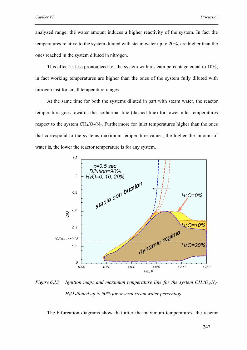
Capther VI Discussion
247
analyzed range, the water amount induces a higher reactivity of the system. In fact the
temperatures relative to the system diluted with steam water up to 20%, are higher than the
ones reached in the system diluted in nitrogen.
This effect is less pronounced for the system with a steam percentage equal to 10%,
in fact working temperatures are higher than the ones of the system fully diluted with
nitrogen just for small temperature ranges.
At the same time for both the systems diluted in part with steam water, the reactor
temperature goes towards the isothermal line (dashed line) for lower inlet temperatures
respect to the system CH4/O2/N2. Furthermore for inlet temperatures higher than the ones
that correspond to the systems maximum temperature values, the higher the amount of
water is, the lower the reactor temperature is for any system.
Figure 6.13 Ignition maps and maximum temperature line for the system CH4/O2/N2-
H2O diluted up to 90% for several steam water percentage.
The bifurcation diagrams show that after the maximum temperatures, the reactor

Capther VI Discussion
248
temperature goes down towards the isothermal line and the difference between the reactor
and the isothermal temperature becomes relatively small and it slightly varies with a
further increase of the inlet temperatures. It is possible to identify, for any C/O feed ratios
and any considered system, the maximum temperature reached during the oxidation
process. If these pointed are reported in the ignition maps, for any system it is possible to
draw the line of the maximum temperatures.
Figure 6.14 Ignition maps and maximum temperature line for the system CH4/O2/N2-
H2O diluted up to 90% for several steam water percentage.
The maps and lines in questions are reported in figure 6.13. On the right side of these
lines the reactivity of the system meaningfully diminishes. The figure show that, as the
steam concentration increases, the maximum temperature line is shifted towards lower inlet

Capther VI Discussion
249
temperatures.
Figure 6.14 shows some temporal temperature profiles obtained for C/O=0.1 and
Tin=1100K (a) and for C/O=0.4 and Tin=1300K (b) for the three system discussed in this
paragraph.
Figure 6.14a shows a case of triangular oscillations while figure 6.14b triangular
oscillations with high amplitude.
The presence of steam does not change the oscillation typology and slightly affects
the frequency and the amplitude of oscillations.
Comparison between Numerical and Experimental Results
In the chapter IV several models have been employed to see if the dynamic behavior,
detected experimentally, was predictable by means of numerical analyses. In particular the
models of “Warnatz”, “Nancy”,“Dagaut” and “Ranzi” were employed in these simulations.
.
Figure 6.15 Experimental and numerical map of stability obtained for methane

Capther VI Discussion
250
oxidation in diluted conditions.
As matter of fact, they were able to predict the oscillation phenomenology found out
during experimental tests. The results were resumed in ignition maps reported and
discussed in chapter IV. It is hence possible to compare the experimental and numerical
results on the basis of experimental and numerical ignition maps. They have been obtained
for a system CH4/O2 diluted with nitrogen up to 90% and for a residence time of 0.5 sec.
In the stable combustion region, the dashed-dotted curve, representing the
numerically computed loci of maximum temperature increase for a fixed C/O, quite ably
reproduces the same curve obtained by means of the experimental analysis (dashed line).
Fig.6.15 shows the comparison between the experimental map and the numerical
maps obtained with the “Nancy model” and the “Warnatz” model. For these simulations
the global heat transfer coefficient was equal to 4.4*10-3 cal/cm2 sec K.
The range of parameters where stable combustion occurs is well predicted by the two
models. Furthermore, both of them predict the existence of a zone where oscillations are
present and they reproduced all the kinds of oscillations but irregular and bell-shape ones.
The models are also able to predict double oscillations even though in these conditions the
zone is hardly identifiable on the map because it is very narrow.
The numerical dynamic regions only partially covers the one identified by means of
the experimental analysis. As a matter of fact, both the models fail the prediction in high
temperature range and at high C/O ratios.
Better results have been achieved using the “Ranzi” model. A comparison of the
experimental and the numerical maps is reported in Figure 6.16. The global heat transfer
coefficient was set equal to 2*10-3 cal/cm2 sec K since more thorough calculations showed
that it was more adapt for the real system used for the experiments
The numerical results demonstrate that the kinetic model is able to reproduce the

Capther VI Discussion
251
system behavior for a significant portion of the dynamic region. For C/O=0.05-0.1, the
oscillations are present in the 1030K to 1275K temperature range. By increasing the C/O,
the dynamic region shrinks, covering a shorter temperature range, and disappears
altogether when the C/O is higher than 0.45. Up to this C/O value, the left-hand boundary
of the region follows that of the experimental dynamic area quite well. In contrast, the right
edge limits the oscillation region to a temperature range that is smaller than the one
corresponding to the experimental area.
The numerical model is also able to predict different oscillation typologies. Single
oscillations occur across most of the dynamic area, but, in contrast with the two other
models, it was also possible to predict double and irregular oscillations and locate them in
a region. Such area develops for temperature comprised 1075K-1160K and for C/O values
between 0.075 and 0.18.
In the stable combustion region, the dashed-dotted curve, representing the
numerically computed loci of maximum temperature increase for a fixed C/O, quite ably
reproduces the same curve obtained by means of the experimental analysis (dashed line).
Figure 6.16 Comparison between experimental and numerical map at 90% of dilution
level.

Capther VI Discussion
252
In order to compare the numerical results obtained with the other models among
them, new numerical integrations have been realized, since the analyses realized with
“Warnatz” and “Nancy” models were obtained for a different global heat transfer
coefficient. The heat transfer used in these new simulations was 2*10-3 cal/cm2 sec K.
The comparison between the “Warnatz”, “Ranzi” and the experimental ignition maps
is reported in figure 6.17.
As shown in chapter IV, an increase of the global heat transfer coefficient sensibly
reduces the extension of the dynamic region in the temperature range. Hence the
“Warnatz” ignition map, obtained with the new coefficient, is less wide and the agreement
with the experimental data worsens.
The comparison among the maps does not lead to any new results, but it can be seen
that the “Warnatz” model identify a minor number of inlet conditions for which the system
evolves trough a dynamic regime. Furthermore it fails to predict the dynamic behavior for
very high temperatures, relatively to the range analyzed, and lean mixtures.
Figure 6.17 Comparison between experimental and “Warnatz” and “Ranzi” maps at
90% of dilution level.

Capther VI Discussion
253
Moreover the “temperature drop” line shown on the figure does not coincide with the
experimental line. This indicates that the “Warnatz” model does not work properly for rich
mixtures very at high temperatures.
Maybe it is due to the minor amount of species that are involved in the “Warnatz”
model in comparison with the “Ranzi” one. In fact it counts for 34 species, until the
formation of compounds with two carbon atoms, and 164 reactions while the “Ranzi”
mechanism has 250 species implicated in more than 5000 reactions.
Anyway it suggests the idea that, even if the numerical results obtained by means of
the “Warnatz” do not predict properly the experimental behavior of the system, the
oscillations are reproducible, with their main characteristics, considering just the oxidation
and the recombination channel with just C2 species.
Flow diagrams
The good results obtained using the methane oxidation mechanisms have suggested
the possibility of performing new numerical simulations to understand the kinetic
pathways responsible of the insurgence of the dynamic behaviors. To this aim a rate of
production analysis was carried using the “Warnatz” model, because it counts for a minor
number of reactions and species, and hence it is a relatively mechanism to analyze. In such
a way the numerical study can be easier to perform and however can lead to important
basic information concerning the dynamic behavior experimentally recognized.
The rate of production analysis has been realized for an initial condition that
corresponds to a cusp-shape oscillation with a frequency of 0.22 Hz and amplitude of
about 200K. In particular, the Tinlet was fixed at 1050K and C/O at 0.2. The temperature
temporal profile computed in these conditions was reported in Figure 6.18. According to
the definition of cusp-shape oscillation, the first, very weak, temperature increase
represents the first step ignition. After a long induction time, that lasts about 4s, it is

Capther VI Discussion
254
followed by the second ignition step that leads to the maximum oscillation temperature.
Figure 6.18 Cusp-shaped oscillation obtained for C/O=0.2 and Tinlet= 1050K.
The rate of production analysis was performed at different time during the oscillation
period, with particular regard to times closer to the second step ignition. The numeric
results are summarized in species flow diagrams that allow understanding which is the
main oxidation path trough which the methane and oxygen react at any time.
In the flow diagrams, the blocks represent the species, which follow the path
indicated by the arrows. The position of a species on the diagram depends on the type and
the number of atoms that it contains. The hydrogen content in molecules decreases moving
from the top toward the bottom of the diagram. The species with more than one carbon
atom lay on the right side of the scheme whereas the molecules containing oxygen are
reported on the left side of each column representing the evolution of species with the
same carbon atoms. The arrow thickness is proportional to the reaction rate.
The flow diagram obtained for 4.5 sec was reported in Figure 6.19. The thick line
entering the methane block represents the feed that is equal in both the flow diagrams here
considered. Although its thickness was arbitrary chosen, the thickness of all the arrows
emerging from the methane block are scaled in such a way that difference between the
entering and emerging arrows thickness represents the methane conversion. This

Capther VI Discussion
255
consideration applies for each block reported in the flow diagram. Moreover, in flow
diagram equilibrium reaction involving CH3O2 and CH4 is indicated with a different grey
level since it is one order of magnitude thicker than the other arrows.
The flow diagram reported in Figure 6.19 shows that the few radicals available at this
time in the reactor dehydrogenate methane thus producing CH3 that, in turn, mainly reacts
with O2.
Figure 6.19 Species flow diagram obtained for 4.5s
Therefore, the main oxidation path is CH3→CH2O→CHO→CO. All the radicals
OH, H and O produced along this reaction path, come back to the initial step of the chain
and dehydrogenate the methane. Since the oxidation of CO to CO2 is very slow and the
methane conversion is very low, the temperature increases of few degrees. At this time

Capther VI Discussion
256
only the oxidation reaction is active. At higher time, up to 8.7s, HO2 radicals, which can
also lead to the formation of H2O2, mainly oxidize CH3. The decomposition of
hydroperoxy radical, that represents the reaction branching, is very slow in these
conditions, such as occurs for the branching reactions of high temperature regimes. As a
consequence, the system reactivity is very low. Up to this time the recombination
mechanism covers a marginal role.
At the 8.7 sec the system is closer to the second step ignition and its temperature
reaches 1070K. The main reaction path is still the oxidation of the radical CH3 to CH3O
and its dehydrogenation up to CO. The conversion of CO to CO2 increases and the
recombination reaction begins to cover a more important role. The main path of the
r e c o m b i n a t i o n c h a n n e l , i n v o l v i n g C2 s p e c i e s , i s
C2H5→C2H4→C2H3→CH2CHO→CH3CHO→CH3CO. The CH3CO radical, in turn,
decomposes thus producing CH3 and CO.
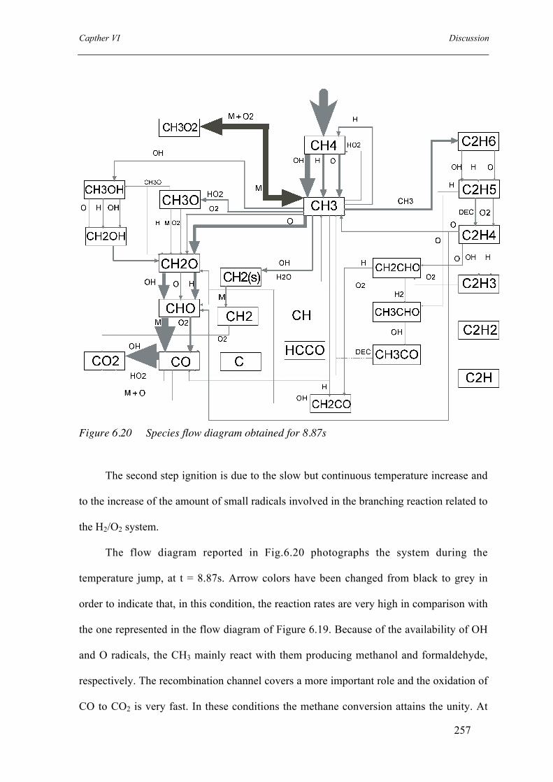
Capther VI Discussion
257
Figure 6.20 Species flow diagram obtained for 8.87s
The second step ignition is due to the slow but continuous temperature increase and
to the increase of the amount of small radicals involved in the branching reaction related to
the H2/O2 system.
The flow diagram reported in Fig.6.20 photographs the system during the
temperature jump, at t = 8.87s. Arrow colors have been changed from black to grey in
order to indicate that, in this condition, the reaction rates are very high in comparison with
the one represented in the flow diagram of Figure 6.19. Because of the availability of OH
and O radicals, the CH3 mainly react with them producing methanol and formaldehyde,
respectively. The recombination channel covers a more important role and the oxidation of
CO to CO2 is very fast. In these conditions the methane conversion attains the unity. At

Capther VI Discussion
258
8.88s the temperature reaches the maximum value of 1240K and then decreases down to
inlet temperature.
In order to understand which reactions play an important rule in the establishment of
oscillatory behavior a further analysis has been done by means of reaction flow analysis. It
was performed by properly changing the “Warnatz” methane oxidation mechanism,
deleting some reactions or changing their kinetic constants.
The rate of production analysis showed that the recombination reactions gain
relevance during the phases of the second step ignition. Therefore, the attention was
focused on the weight of this reaction channel on the oscillation phenomenology. Starting
form the initial conditions considered in the previous simulations, the first analysis was
performed by deleting from the kinetic mechanism the whole recombination channel. The
results were summarized in Figure 6.21 where the temperature profiles obtained with the
original and modified model were reported. In figure 6.21b it can be easily seen that the
closure of the recombination reaction path leads to an increase of oscillation frequency that
passes from 0.2Hz up to 1.6Hz.
The opposite effect was obtained by increasing the velocity of CH3 recombination.

Capther VI Discussion
259
Figure 6.21 Temperature profiles computed the original and modified models
In particular, the activation energy of this reaction was decreased from 81240 J/mole
to 70000 J/mole. In this case the oscillation phenomenology disappears leading to a stable
temperature profile as shown in figure 6.21c. These results suggest that a faster
recombination channel removes CH3 radicals from the oxidation channel. Therefore, these

Capther VI Discussion
260
radicals pass trough reactions that are slower in comparison with the reactions of the other
“competitive” channel and at the same time they are not able to provide the same amount
of radicals. The system pays this lack with a lower reactivity. Furthermore, the CH3CO
decomposition, which produces CH3 and CO making them available for oxidation, is very
slow. This results in a CH3 radicals trapping in the recombination channel.
The same effect can be obtained by suppressing the CH3CO decomposition from the
initial model, such as shown by the temperature profile reported in Figure 6.21d. Again,
the recombination channel removes CH3 radicals that are not made available again due to
the absence of CH3CO decomposition.
This mechanism seems to give also a plausible explanation for the observed increase
of frequency by increasing the inlet temperature, at a fixed C/O ratio. As a matter of fact,
the less the inlet temperature is, the later the second step ignition will be favored. This
means that the amount of CH3 stored by the recombination channel will be greater.
Therefore, when the conditions favor the second step ignition, the reactivity of the system
will be higher. It means the oscillation regime will have low frequency values but high
temperature gradients. On the other hand the higher the temperature is, the faster the
oxidation channel will win the competition with the recombination channel. This means
the system will have a shorter time to store the radical CH3 so when the ignition occurs the
system will evolve trough oscillatory regimes with a higher frequency but a lower
temperature gradient.
By this way the recombination channel is able to module the frequency of the
oscillation regimes and so the temperature gradient.
In order to verify the consideration reported above in a wider range of parameters,
the same analysis was carried out both in higher temperatures and richer feed ratios. The
results confirmed the crucial role of the recombination pathway in dynamic evolution of

Capther VI Discussion
261
the system. As matter of fact it coherently responds to the same model modifications.
In figure 6.22 it is reported a scheme of the main pathways active in the oxidation
scheme of methane. Several radicals, such as OH, H and O; firstly dehydrogenate methane
to CH3. Methyl radical can pass trough the oxidation pathways until the formation of CO
or CO2 or can recombinate and form ethane. This compound can be farther on
dehydrogenated, by means of radicals or thermal decompositions, to form several species
until the vinyl radical (C2H3). It can oxidize with the formation of oxygenated species or
can dehydrogenises, yielding C2H2.
Figure 6.22 Reaction scheme of methane.
The rates of reactions responsible for C2H3 consumption have been evaluated as
function of Tinlet. The results at C/O=0.5 were reported in Figure 6.23a where the dashed
curve represents the rate of C2H3 oxidation whereas the solid line indicates the rate of C2H3
dehydrogenation to C2H2. The rate of C2H3 oxidation increases up to Tinlet=1175K. As
shown by dashed-dotted line in Figure 6.23b, this temperature corresponds to the highest
ΔT computed at C/O=0.5. In the same temperature region, the rate of C2H3

Capther VI Discussion
262
dehydrogenation increases continuously with Tinlet although it always remains lower than
C2H3 oxidation rate. From Tinlet=1175K onwards, the rate of C2H3 oxidation decreases and
is overwhelmed at about Tinlet=1275K by C2H3 dehydrogenation which continues to rise.
Figure 6.23 C2H3 reaction rate for oxidation and dehydrogenation channel at C/O=0.5
and C/O=0.1
The same analysis was performed for C/O=0.1, i.e. under lean conditions. From
Tinlet=1000K up to Tinlet=1050K, C2H3 oxidation is the only active channel of C2H3
consumption. It reaches an initial maximum at Tinlet=1025K then decreases up to
Tinlet=1050K. Higher Tinlet corresponds to a temperature oscillation region, where the
reaction rates represent the mean value computed for a single oscillation period. With the
onset of oscillation, both oxidation and dehydrogenation reactions increase. The former
reaches a maximum at 1150K, then decreases but still remain higher than the C2H3
dehydrogenation rate. At Tinlet=1050K, the C2H3 dehydrogenation rate suddenly reaches a
nearly constant value and remains that way until 1300K before falling steeply to very low
values.

Capther VI Discussion
263
Hydrogen Addiction: Rate of Species Production Analysis
To identify the hydrogen addition effect on the kinetic paths of methane oxidation, a
rate-of-production analysis was carried out for Tin equal to 1015 K and for a C/O ratio
value equal to 0.2. Fig. 6.24 shows the effect of the hydrogen addition on the temperature
temporal profiles predicted by the “Warnatz” model.
Figure 6.24 Hydrogen addition effect on the ignition kinetic mechanism of the system for
Tin=1015 K and C/O=0.2.
To identify the hydrogen addition effect on the kinetic paths of methane oxidation, a
rate-of-production analysis was carried out for Tin equal to 1015 K and for a C/O ratio
value equal to 0.2. Fig. 6.24 shows the effect of the hydrogen addition on the temperature
temporal profiles predicted by the “Warnatz” model.
An addiction of hydrogen to the system CH4/O2/N2 leads the system to pass from a
slow combustion to an oscillating regime. The analysis was performed at 0.2 sec after the
beginning of the simulation.
Analyses realized in absence of hydrogen show that for the chosen inlet conditions
the main branching reaction might be the decomposition of the H2O2. H atoms react via the
breaking reaction H+O2+M_HO2+M producing the relatively stable HO2 radicals. They

Capther VI Discussion
264
form H2O2 that decomposes into two OH radicals.
The presence of hydrogen promotes the high temperature classical branching
reactions and increases the whole reactivity of the system. In fact H2 reacts mainly with
OH through the exothermic reaction H+O2_OH+O. From the rate-of-production analysis it
has come out that reactions that involve the radical OH show the most significant
increment. For H2 concentration equal to 0.9% also the breaching reaction H2+O_OH+H
becomes significant in the production of OH radicals. They mainly dehydrogenate the
methane to CH3. In such a way the oxidation pathways of methane can be initialized and
accelerated by the great amount of radicals present in the system. These kinetic paths are
resumed in the flow diagram reported in figure 6.25. The thickness of the arrows is
proportional to the rate of the several reactions reported in the scheme. This diagram is
relative to a hydrogen inlet concentration equal to 0.9%.
Figure 6.25 Main kinetic paths involved in the ignition mechanism of the CH4-H2/O2/N2
system in presence of hydrogen for Tin=1015 K and C/O=0.2 at the time
t=0.2 s.
The effect of hydrogen addiction is very similar to the effect that has been obtained

Capther VI Discussion
265
by removing the recombination channel from the “Warnatz” model as reported in chapter
V.
The numerical analysis consisted in properly changing the “Warnatz” methane
oxidation mechanism, deleting some reactions or changing their kinetic constants. It was
performed for a system composed by methane and oxygen diluted up to 90% by nitrogen.
The temperature was 1050K and the C/O feed ratio was 0.2.
The results have been summarized in Figure 6.26 where the temperature profiles
obtained with the original and modified model were reported. Using the original
“Warnatz” model for the inlet conditions analyzed the system evolves trough a cusp-
shaped oscillating regime.
In figure 6.26b it can be easily seen that the closure of the recombination reaction
path leads to an increase of oscillation frequency that passes from 0.2Hz up to 1.6Hz.
This is mainly due to the fact that CH3 radical cannot pass trough the recombination
channel, hence they just can go trough the recombination channel thus they feed such
pathway in a more consistent way and also the radicals, produced in the oxidation channel
from CH3 to CO, are consumed just in this pathway. It results in a higher reactivity of the
system.
The opposite effect was obtained by increasing the velocity of CH3 recombination. In
particular, the activation energy of this reaction was decreased from 81240 J/mole to
70000 J/mole. In this case the oscillation phenomenology disappears leading to a stable
temperature profile as shown in figure 6.26c. These results suggest that a faster
recombination channel removes CH3 radicals from the oxidation channel. Therefore, these
radicals pass trough reactions that are slower in comparison with the reactions of the other
“competitive” channel. At the same time, they are not able to provide the same amount of
radicals and the dehydrogenation reactions, typical of the recombination channel, consume

Capther VI Discussion
266
the radicals present in the system. The system pays this lack with a lower reactivity.
Furthermore, the CH3CO decomposition, which produces CH3 and CO making them
available for oxidation, is very slow. This results in a CH3 radicals trapping in the
recombination channel.
The same effect can be obtained by suppressing the CH3CO decomposition from the
initial model, such as shown by the temperature profile reported in Figure 6.26d. Again,
the recombination channel removes CH3 radicals that are not made available again due to
the absence of CH3CO decomposition.
Therefore, if the attention is focused on the figure 6.26a and 6.26b, it appears that the
hydrogen addiction promotes the oxidation channel and leads the system to oscillate.

Capther VI Discussion
267
Figure 6.26 Temperature profiles computed the original and modified “Warnatz”
models.
Furthermore, an analysis realized on the reaction rates of the reactions that promote
the chain mechanism, and hence sustain the combustion process, appeared clear that during
the temperature jump the branching reactions are the reactions of the system H2/O2 typical
of high temperatures. The results are shown in figure 6.27. This analysis has been realized
for the same inlet conditions considered in the sensitivity analysis.
In particular for low temperatures the main branching reaction is the decomposition

Capther VI Discussion
268
of the hydrogen peroxide (reaction 1). It causes the first temperature step.
H2O2 + M γ OH + OH + M
1)
Then there is an induction time before the temperature jump occurs. In this period the
most important reactions is reaction (reaction 2).
H + O2 + M γ HO2 + O + M
2)
HO2 radicals react and form the hydrogen peroxide that decomposes and provides for
OH radicals.
When there is an enough high amount of radicals the system reach the condition to
realize the second temperature jump. The temperatures become sufficiently high to
promote the chain radical mechanism of the system H2/O2 typical of high temperatures
(reaction 3 and 4)
H + O2 γ OH + O 3)
H2 + O γ OH + H 4)
Figure 6.27 Rates of the reactions 1), 2) and 3)
Since a hydrogen addiction promotes the formation of radicals H, O and OH,
enhancing the reaction rates of the reactions 3) and 4), as shown in figure 6.25, it is clear

Capther VI Discussion
269
that the oxidation channel becomes more important.
In figure 6.28 it is reported the diagram relative to the methane yield in CO, CO2,
C2H2 obtained by means of the “Dagaut” mechanism for a C/O feed ratio equal to 0.6 and
an inlet temperature equal to T0= 1175 K.
For these inlet conditions, the model predict that higher reactor temperatures with
increasing the hydrogen percentage.
As matter of fact, the system with an inlet hydrogen concentration equal to 2.5%
leads the methane conversion to be almost twice the methane conversion of the system
CH4/O2/N2. The conversion does not increase with a linear law as function of the hydrogen
concentration, in fact for the cases H2=0.5%, 0.75% and 0.9% the conversion is
respectively 36%, 42% and 39%.
This trend is mainly due to the fact that hydrogen can react with the methyl radical to
produce methane. Hence the conversion of methane is lowered by the hydrogen addiction
but methyl radicals that pass trough the oxidation channel, can be easily oxidized to CO
and CO2 since the amount of radical is enhanced by the presence of hydrogen.
This is also understandable considering the increase of methane yield in CO, CO2
and C2H2. Also in this case they increase with a non-proportional law as function of the
hydrogen concentration.
In particular the CO2 yield increase from 9% to 17%. This justifies the higher reactor
temperatures numerically obtained for the systems with hydrogen. As mater of fact, the
reaction of carbon monoxide to carbon dioxide is the most exothermic reaction of the
methane kinetic mechanism, thus it implicates higher working temperatures.
An important aspect of the hydrogen addiction to the system CH4/O2/N2 is the higher
yield of methane in C2H2. It has been underlined that the higher the working temperature
is, the higher the acetylene stability is. In particular for temperature higher than about

Capther VI Discussion
270
1200K the acetylene starts becoming a stable species.
Furthermore the hydrogen presence, as explained in chapter II, increases the
formation of acetylene and slows down the formation of species such as ethane, benzene
and carbon coke. Hence the stability of C2H2 is improved by hydrogen addiction.
Furthermore the relative low partial pressure of methane and the relatively high
temperatures favor the formation of acetylene instead of benzene and ethene.
Hydrogen interacts both in the oxidation and recombination channels leading to a
higher reactivity for low inlet temperatures, but it damps the reactivity of the system for
high working temperatures and rich mixtures favoring, in the mean time, the formation of
acetylene.
Figure 6.28 Methane yield diagram in CO, CO2, C2H2 obtained for the “Dagaut”
mechanism for C/O=0.6 and Tin= 1175K

Capther VI Discussion
271
Discussion
This could explain the “temperature drop” behavior that has been explained in the
experimental bifurcation diagram. In fact, the possibility to produce acetylene represents
the capacity of the system to store carbon and hydrogen atoms and subtract them to the
oxidation channel. Hence, if hydrogen enhances the availability of radical species and
induce the system to work with higher temperatures, and higher yields, from the other side,
it favors the thermodynamic stability of the acetylene, thus, for certain working conditions,
depending on the inlet temperatures and mixture composition, it slows down the oxidation
reactions.
Steam Water: Chemical Effect
In the Chapter IV it has been reported a numerical study realized to characterize the
system CH4/O2 diluted with steam water and nitrogen up to 90% for several steam
concentrations, in terms of species produced during the methane oxidation process. Hence
the fuel conversion and its yields into carbon oxide, carbon dioxide and C2 products have
been calculated. The study has revealed that, increasing the steam concentration; the
methane conversion towards CO2 increases, while the CO production decreases. In order to
better understand the effect of water addition to the system CH4/O2 further numerical
simulations have been realized.
The analysis has the aim to discriminate the thermal and chemical contribution of
steam water to the evolution of the methane oxidation process in Mild conditions. In
literature is in fact known that water can act in two different ways: a thermal and a
chemical effect. The former is mainly due to its higher capacity in comparison with
nitrogen, hence it can lower the working temperature causing a reduction of reaction rates

Capther VI Discussion
272
involved in the oxidation process. The latter effect is due to its higher efficiency as third-
body in third molecular reactions, in comparison with nitrogen. Hence water can induce an
enhancement of the rate of third molecular reactions, such as terminating ones.
Furthermore water is not an inert species, thus it can breakdown causing an increase of
radical species.
In order to clarify and separate the contribution of the two effects just illustrated,
during the numerical simulations it has been defined a species X that has the same heat
capacity and the same efficiency of water but it is an inert species. As matter of fact this
species is not involved in the elementary reactions of the methane oxidation kinetic
mechanism. To this aim the “Warnatz” model has been modified.
Results are shown in the following figures. In particular in figure 6.29 the methane
conversion for the systems CH4/O2 diluted with N2 and steam are reported. In particular
steam has been added in such a way that nitrogen and steam dilute the system up to 90%.
Steam percentage has been set equal to 0, 10% and 20% of the overall dilution degree.
Then methane conversion is compared with the ones of the systems in which steam water
has been substituted with the inert species X.
The analyses has been realized in a temperature range that goes from 1000K to
1700K for a rich mixture, in which the C/O feed ratio is equal to 0.4.
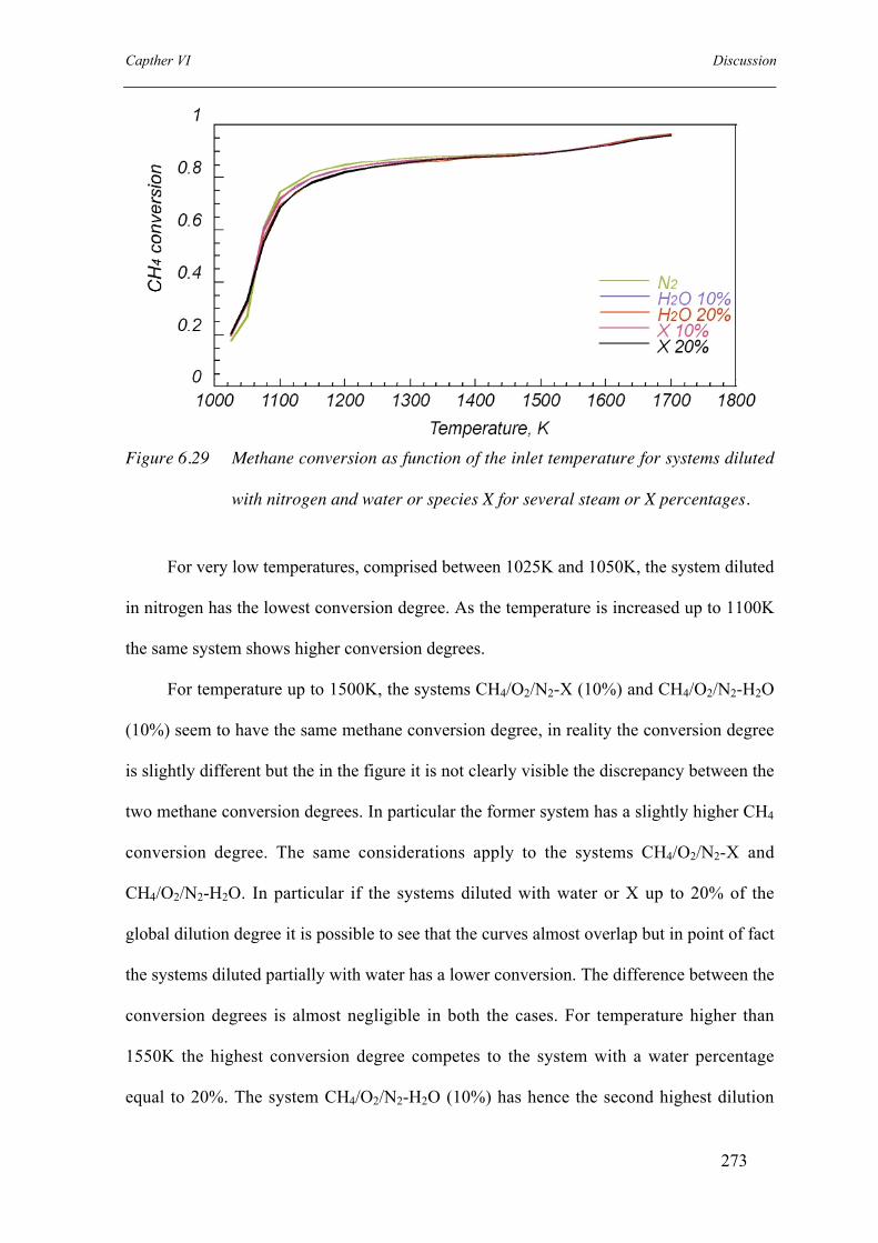
Capther VI Discussion
273
Figure 6.29 Methane conversion as function of the inlet temperature for systems diluted
with nitrogen and water or species X for several steam or X percentages.
For very low temperatures, comprised between 1025K and 1050K, the system diluted
in nitrogen has the lowest conversion degree. As the temperature is increased up to 1100K
the same system shows higher conversion degrees.
For temperature up to 1500K, the systems CH4/O2/N2-X (10%) and CH4/O2/N2-H2O
(10%) seem to have the same methane conversion degree, in reality the conversion degree
is slightly different but the in the figure it is not clearly visible the discrepancy between the
two methane conversion degrees. In particular the former system has a slightly higher CH4
conversion degree. The same considerations apply to the systems CH4/O2/N2-X and
CH4/O2/N2-H2O. In particular if the systems diluted with water or X up to 20% of the
global dilution degree it is possible to see that the curves almost overlap but in point of fact
the systems diluted partially with water has a lower conversion. The difference between the
conversion degrees is almost negligible in both the cases. For temperature higher than
1550K the highest conversion degree competes to the system with a water percentage
equal to 20%. The system CH4/O2/N2-H2O (10%) has hence the second highest dilution

Capther VI Discussion
274
degree while for the other systems curves overlap.
The effect of water on the methane conversion is not very evident since the methane
conversion and temperatures reached by the systems are very close to each other. More
meaningful information can be obtained considering the methane yield into CO2 and CO.
Figure 6.30 CO2 yield as function of the inlet temperature for systems diluted with
nitrogen and water or species X for several steam or X percentages.
Figure 6.30 shows the conversion of methane into carbon dioxide as function of the
inlet temperature for the several systems considered in the numerical analysis.
It is here evident that the highest value of the discussed parameter competes to the
system CH4/O2/N2-H2O (20%). In fact it has the highest value for temperatures higher than
1100K, and it reaches a value equal to about 0.58 for an inlet temperature equal to 1700K.
The system CH4/O2/N2-H2O (10%) has the second highest CO2 yield. The curves
relative to the other considered systems overlap.
It is worth noting that the curve relative to the system CH4/O2/N2-H2O (10%) reaches
a plateau, while in the other cases the CO2 yield curves pass trough a maximum value and
then slowly decrease.

Capther VI Discussion
275
Figure 6.31 shows the conversion of methane in CO as function of inlet temperature
for systems diluted with nitrogen and water or X, for several steam or X percentages.
In this case the system diluted in nitrogen presents the highest values of the
parameter CO yield. The conversion significantly lowers for the systems diluted in
nitrogen and water. The systems CH4/O2/N2-X (10%) and CH4/O2/N2-X (20%) show a
methane yield into CO slightly different from the system diluted just with nitrogen. In
theses cases curves overlap for very high inlet temperatures. Furthermore the higher the
concentration of X is, the lower the CO yield is.
In this case it is possible to identify the chemical contribute of water addiction. The
species X and steam water, takes part to the kinetic reaction mechanism of methane in
different ways, in particular they participate in the same way in third molecular reactions
as third-body but the species X can not dissociate or react in other way, while water can
give rise to breakdown reactions. Hence the gap between the curves relative to the species
X and the steam water, for a fixed concentration, clearly indicates the chemical effect of
water. The main effect on the kinetic evolution of the methane oxidation is that steam acts
in such a way to increase the conversion of methane to CO2 while decreasing the
conversion to CO.

Capther VI Discussion
276
Figure 6.31 CO yield as function of the inlet temperature for systems diluted with
nitrogen and water or species X for several steam or X percentages.
Figure 6.32 shows the methane conversion in acetylene as function of the inlet
temperature for the systems CH4/O2/N2, CH4/O2/N2-H2O (10%-20%) and CH4/O2/N2-X
(10%-20%). The figure shows that in any system acetylene increases as the inlet
temperature is increased, reaches a maximum and quickly diminishes. The system diluted
in nitrogen and water, with a steam relative percentage equal to 20%, present the highest
values of methane conversion in C2H2 until a value of the temperature equal to 1500K,
then it reaches a maximum and decreases. The curve relative to the system CH4/O2/N2-H2O
(10%) shows that same trend, but it has a maximum for an inlet temperature equal to
1600K.
In correspondence of these maximum values, the C2H2 yield of the other systems
overcomes the ones relative to the systems diluted in nitrogen and water. In the other cases
curves almost coincide. For temperatures lower than 1400K the system diluted in nitrogen
shows a slightly higher production of acetylene in comparison with the systems diluted in
nitrogen and X. In this case the higher is the X species concentration, the lower is the
methane conversion in acetylene.

Capther VI Discussion
277
Figure 6.32 C2H2 yield as function of the inlet temperature for systems diluted with
nitrogen and water or species X for several steam or X percentages.
For temperatures lower than 1400K the acetylene production curves invert their
relative position and the system diluted in nitrogen shows the lowest acetylene yield while
the highest one competes to the system CH4/O2/N2-X (20%). The discrepancy among
values for the systems CH4/O2/N2-X (10%-20%) and CH4/O2/N2 is very small.
Other simulations have been run to understand the effect of steam on methane
oxidation in Mild condition. In particular higher steam percentages; up to 50% and 100%,
have been used. These high steam concentrations have been used in order to make more
evident the effect of vapor water on the system analyzed. Figure 6.33 shows the reactor
temperature as function of the inlet temperatures for the system diluted in nitrogen and
water with a steam concentration equal to 0%, 10%, 20%, 50% and 100%. The reactor
temperature is not significantly affected by the presence of water in the several percentage
reported above. In fact all the curves almost overlie. The difference among the
temperatures is just of few degrees.
Figure 6.34 shows the methane conversion as function of the inlet temperature for

Capther VI Discussion
278
the systems taken in consideration.
Figure 6.33 Reactor Temperature as function of the inlet temperature for systems
diluted with nitrogen and water for several steam percentages.
Figure 6.34 Methane conversion as function of the inlet temperature for systems diluted
with nitrogen and water for several steam percentages.
In this case in the temperature range comprised between 1050K and 1460K the
system diluted in nitrogen presents the highest conversion. It is identifiable a clear trend of

Capther VI Discussion
279
the methane conversion, in fact as the steam concentration increases the methane
conversion decreases. For an inlet temperature equal to 1460K, curves intersect and for
higher temperatures they invert their relative position. In this case an opposite trend,
respect to the one just discussed above, is recognizable, in fact the higher the steam
concentration is, the higher methane conversions are.
Figure 6.35 shows the methane conversion in carbon dioxide as function of the inlet
temperature for the systems diluted in nitrogen and water.
Figure 6.35 CO2 yield as function of the inlet temperature for systems diluted with
nitrogen and water for several steam percentages.
Except for very low temperatures, relative to the range analyzed in these numerical
simulations, the highest CO2 yield competes to the system fully diluted with steam water.
Decreasing the steam concentration in the systems CH4/O2/N2-H2O the methane
conversion in carbon dioxide lowers.
In particular the conversion degree is 0.8 for a steam percentage equal to 100%, then
it becomes 0.7, 0.55, 0.45 and 0.3. Furthermore the CO2 yield curves increases
monotonically for the two systems that have the highest steam amount. In the other cases

Capther VI Discussion
280
the CO2 yield reaches a maximum and than slowly decreases. The maximum value is
gained by the systems for lower inlet temperatures as the steam concentration decreases.
An opposite trend is identifiable for the methane conversion in carbon monoxide.
Figure 6.36 shows such a yield as function of the inlet temperature for the systems diluted
up to 90% with nitrogen and water for several diluent compositions. In this cases the
higher the steam concentration is, the lower the CO yield is.
The several curves show a similar trend: the CO yields firstly quickly increase, pass
trough a maximum value, than decrease reaching a relative minimum value, finally
increase again.
Figure 6.36 CO2 yield as function of the inlet temperature for systems diluted with
nitrogen and water for several steam percentages.
Both the maximum and the minimum values occur for lower inlet temperatures as the
steam amount is enhanced.
Figure 6.37 reports the acetylene yield as function of the inlet temperature for
systems diluted with nitrogen and water for several steam percentages. Curves show that

Capther VI Discussion
281
the methane conversion in acetylene increases as function of the inlet temperatures, reacha
maximum and decrease.
Figure 6.37 C2H2 yield as function of the inlet temperature for systems diluted with
nitrogen and water for several steam percentages.
The maximum occur for lower inlet temperatures and has a lower value as the steam
concentration is increased. In fact for the system completely diluted in steam it occurs for
an inlet temperature equal to 1440K, while for the system diluted in nitrogen it seems to
occur for 1700K.
The results obtained using the “Warnatz” model have been compared to the ones
found out using another methane kinetic oxidation mechanism, the “Dagaut” model, that
has been used in other sections to study the effect of hydrogen on the system CH4/O2/N2.
Figure 6.38 shows the reactor temperature as function of the inlet one for the systems
CH4/O2/N2, CH4/O2/N2-H2O (10%), CH4/O2/N2-H2O (20%) for the two used models. In the
legend of the figure the “W” indicates data from the “Warnatz” model while “D” from the
“Dagaut” one.
It can be seen that the reactor temperatures relative to the same kinetic model overlie,

Capther VI Discussion
282
while data from the two models show that the second oxidation mechanism predicts lower
temperatures for low inlet temperatures. In particular the “Dagaut” model for temperatures
up to 1125K indicates that the system is not able to ignite. Once the methane oxidation
reactions start, the reactor temperatures for the two models match. In fact for inlet
temperatures higher than 1175K lines overlap.
Figure 6.38 Reactor Temperature as function of the inlet temperature for systems
diluted with nitrogen and water predicted by the “Warnatz” and the
“Dagaut” models.
Figure 6.39 shows the conversion of methane as function of the inlet temperatures
predicted by the two models. The “Warnatz” model forecasts higher conversion degrees
for inlet temperature lower than 1200K since the mixtures ignite for lower inlet
temperature respect to the other model. But for inlet temperatures higher than 1300K the
“Dagaut” model predicts higher values of methane conversion. Anyway it is confirmed the
trend discussed earlier in the same paragraph. The system diluted in nitrogen has a higher
conversion for low temperatures, but as the inlet temperature increases the curves intersect
and they change their relative position indicating that, in the system diluted in nitrogen and

Capther VI Discussion
283
water with a percentage equal to 20%, fuel is more efficiently consumed.
The “Dagaut” results confirm also the trend of the methane conversion into CO2 and
CO observed in a first analysis realized by means of the “Warnatz” model. Figures 6.40
and 6.41 show the CO2 and CO yields predicted by the two models as function of the inlet
temperatures.
Figure 6.39 Methane conversion as function of the inlet temperature for systems diluted
with nitrogen and water predicted by the “Warnatz” and the “Dagaut”
models.
The highest carbon dioxide yields compete to the system diluted in water up to 20%.
In particular for such a system, the “Warnatz” model forecasts higher inlet methane
conversion for temperature up to about 1140K respect to the results obtained by the other
model. For the system CH4/O2/N2-H2O (10%) the “Warnatz” model, once again, indicates
higher conversion degree, but for temperatures higher than 1420K the CO2 yield curves
overlie. On the contrary, for the system diluted just in nitrogen the “Warnatz” model
predicts CO2 yields higher than the ones numerically found out by means of the other
kinetic model, in all the analyzed temperature range.

Capther VI Discussion
284
The CO yields curves obtained by the “Dagaut” model validate the trend already
identified earlier in the analyses realized by means of the “Warnatz” model and earlier
discussed. The curves present a maximum, than a relative minimum and than slowly
increase again. Furthermore the higher the steam concentration is, the lower the CO
production is.
However, comparing the several systems once the diluent composition has been
fixed, the “Dagaut” model predicts higher methane conversion to this species for high
temperatures, while for low temperatures they become lower in comparison to the one
obtained by the other models. In particular curves relative to the system CH4/O2/N2, come
across for an inlet temperature equal to 1300K. After this value the CO yields obtained by
the “Dagaut” model overcome the ones got by the “Warnatz” model.
Figure 6.40 Reactor Temperature as function of the inlet temperature for systems
diluted with nitrogen and water predicted by the “Warnatz” and the
“Dagaut” models.

Capther VI Discussion
285
Figure 6.41 Reactor Temperature as function of the inlet temperature for systems
diluted with nitrogen and water predicted by the “Warnatz” and the
“Dagaut” models.
Similar considerations apply for the other systems, even if the intersection between
curves happens for lower inlet temperatures as the steam percentage increases.
Figure 6.42 shows the acetylene production predicted by means of the two models as
function of the inlet temperature for the several considered systems.
In this case comparing the data from the two kinetic models some differences are
identifiable. In fact in general both the models predicts that the systems with steam have a
slightly higher values of the C2H2 yields. Acetylene yield increases, reaches a maximum
and decreases.
The “Warnatz” model indicates that the maximum values significantly change with
the diluent composition, in particular a higher steam concentration implies a lower
maximum, additionally it leads the systems to reach its maximum in acetylene production
for lower inlet temperatures. This last feature is confirmed by data obtained with the
“Dagaut” model but the maximum values are comparable among them.

Capther VI Discussion
286
Indeed the new numerical simulations clearly confirm the trend in methane
consumption and species production obtained with the “Warnatz” model, even if some
differences occur.
Figure 6.42 Reactor Temperature as function of the inlet temperature for systems
diluted with nitrogen and water predicted by the “Warnatz” and the
“Dagaut” models.
The steam water dilution causes hence a reduction in methane conversion for
temperature the low temperatures (T<1450K according to the “Dagaut” model, T<1500K
according to the “Warnatz” model), while for high temperatures the trend is inverted, a
higher conversion of methane to CO2 at detriment of a lower conversion in CO, finally a
shift of the maximum acetylene production towards lower inlet temperatures.
Rate of production analysis
In order to comprehend what reactions are more affected by the presence of great
amounts of steam water a rate of production analysis has been realized using the
“Warnatz” model for the systems CH4/O2/N2-H2O with several steam dilution percentages
(from 0% to 100%). The analysis has been carried out for a C/O feed ratio equal to 0.4 and

Capther VI Discussion
287
an inlet temperature equal to 1200K. This value has been chosen since the discrepancy
between the methane conversion and CO and CO2 yields for the various systems is here
consistent.
Figure 6.43 Reaction rates of methane as function of the composition of the diluent in
the system CH4/O2/N2-H2O.
The rate of production analysis has been realized identifying the most influential
reactions of the methane oxidation mechanism and the attention has been focused on some
key species such as methane, methyl radical, CO and radicals H, O, OH and HO2. Results
have been reassumed in histograms.
Figure 6.43 shows the most important elementary reactions that methane involve
methane net consumption. It is consumed by the following reactions:
CH4 + H =H2 +CH3
CH4 + O = OH + CH3

Capther VI Discussion
288
CH4 + OH = CH3 +H2
and mainly produced by the following reactions:
CH3 + H = CH4
CH3 +HO2 = CH4 +OH
In the system diluted just in nitrogen methane is mainly dehydrogenated to methyl
radicals buy reaction 1), than reaction 3) followed by reaction 2). While the most important
reaction in the methane production is reactions 4).
It can be observed that increasing water concentration the reaction 1) and 2) become
increasingly slower, while the rate of reaction 3) is significantly enhanced. At the same
time reaction 4) becomes slower, while reaction 5) faster. For the system completely
diluted in steam water, the fastest dehydrogenation reaction is reaction 3) followed by
reaction 1) and 2). Hence it seems that all the reactions that involve radicals H and O
become slower, while reactions that involve OH and HO2 radicals become faster as steam
concentration is augmented.
Figure 6.44 shows the most important reactions for the methyl radical as function of
the diluent composition. Methyl radicals are mainly produced by the reactions 1), 2) and 3)
reported above. It is consumed mainly by these reactions:
4) CH3 + H = CH4
CH3 + CH3 = C2H6
CH3 + HO2 = CH3O + OH.
The same considerations realized for the methane reactions relative to reactions 1),
2), 3), 4) and 5) can be repeated for the methyl radicals. Furthermore the rate of reaction
6), that leads to the formation of ethane, is lowered by the presence of steam.
It means that the methyl radicals, as steam concentration is enhanced, prefer going
towards the oxidation channel more than towards the recombination channel.

Capther VI Discussion
289
Figure 6.44 Reaction rates of methyl radicals as function of the composition of the
diluent in the system CH4/O2/N2-H2O.
Figure 6.45 Reaction rates of CO as function of the composition of the diluent in the
system CH4/O2/N2-H2O.

Capther VI Discussion
290
Figure 6.45 reports the reaction rates of CO as function of the composition of the
diluent in the system CH4/O2/N2-H2O. Reactions that produce CO are the following:
CHO + M =CO +H+ M
CH3CO = CH3 +CO
While reaction that consume this species are:
CO +OH =CO2 +H
CO + HO2 = CO2 + OH
It is clear that steam dilution enhances the velocity of the reaction 8), 10) and 11)
while reduce the rate of reaction 9). Reaction 8) becomes faster since water has a very high
third body efficiency in third-molecular reactions in comparison with nitrogen.
Figure 6.46 Reaction rates of H2O as function of the composition of the diluent in the
system CH4/O2/N2-H2O.
In fact in the “Warnatz” kinetic model the nitrogen efficiency for this reaction is 4,
while for steam water it is 6.5. Reaction 10) and 11) becomes faster in presence of steam

Capther VI Discussion
291
water in a manner proportional to water concentration, showing again that reaction that
involve OH and HO2 radical becomes faster.
The next step in this analysis has been the identification of reactions that involve the
steam water itself. Figure 6.46 shows the reaction rates of H2O as function of the
composition of the diluent in the system CH4/O2/N2-H2O.
In the system entirely diluted in nitrogen the main reaction that produce water is the
reaction 3) together with the following reactions:
H2 + OH = H2O + H
C2H4 +OH = C2H3 + H2O
C2H6 + OH = C2H5 +H2O
CH2O + OH = CHO +H2O
And it consumed by reaction
OH + OH =H2O + O
CH2 (S) +H2O _ CH3 +OH
Steam water meaningfully affects the rate of reaction 12) as well as 16). Hence it
affects the equilibrium of reaction 12), and produce OH radicals by reaction 16). Moreover
reactions 15) and 3), as well as13) and 14), become faster and faster. All these reactions
involve OH radicals.
Figure 6.47 reports the main elementary reaction rate of the production and
consumption of molecular hydrogen.
It is produced by reaction 1) and the other reactions ranked below:
CH2O + H = CHO +H2
C2H4 + H = C2H3 + H2
C2H6 + H = C2H5 +H2
It is than produced by reaction 12) and 21):

Capther VI Discussion
292
21) H2 + O = OH +H
The figure 6.47 suggests that all the reactions that involve molecular hydrogen
become less important as the steam percentage increases.
Figure 6.47 Reaction rates of H2 as function of the composition of the diluent in the
system CH4/O2/N2-H2O.

Capther VI Discussion
293
Figure 6.48 Reaction rates of H as function of the composition of the diluent in the
system CH4/O2/N2-H2O.
At the light of these results it emerges that water acts increasing the rate of third-
molecular reactions, since its highest efficiency as third-body species, in comparison with
nitrogen, and of reaction 16) (OH + OH = H2O + O) thus enhancing the production of OH
radicals. Rates of reactions that involve these radicals are enhanced and at the same time
the reactions that involve O, and H radicals slow down.
Indeed the steam significantly affects the evolution of the whole oxidation process.
Since it is mainly based on radical branching reactions, in order to further characterize the
effect of steam, it can be interesting to observe the vicissitude of H, O and OH radicals.
Figure 6.48 shows the reactions relative to the radical H. Reactions that produce H
radicals are reported below:
8) CHO + M =CO +H+ M

Capther VI Discussion
294
10) CO +OH =CO2 +H
12) H2 + OH = H2O + H
H2 + O = OH +H
22) CH3O + M = CH2O + H +M
23) C2H5 = C2H4 + H
while it is consumed by these reactions:
CH4 + H =H2 +CH3
4) CH3 + H = CH4
18) CH2O + H = CHO +H2
19) C2H4 + H = C2H3 + H2
20) C2H6 + H = C2H5 +H2
24) O2 + H = OH + O
25) O2 + H + M = HO2 + M
26) HO2 + H = OH + OH
Also in this case it is clear that the rate of reactions that involve H radicals decrease
in a proportional way respect to the steam concentrations (18, 4, 1, 19, 20). On the contrary
reactions that involve HO2 radicals (26) or a third- body M (22, 25) have a higher
importance in the methane oxidation process in these operative conditions.
In particular it is very important to see how water acts on the branching reactions.
The reactions that lead to a huge amount of radicals, as explained in chapter II, are the
reactions 21), 24) and 12). When reaction 24) starts it is followed by the reactions 12) and
21). They enhance the pool of radicals thus the reactivity of the system. Reaction 24) can
compete with the breaking reaction (25); this reaction leads to the formation of HO2
radicals that are less reactive that radicals OH. If reaction 25) is favored respect the chain
branching reactions (24, 12, 21) the reactivity of the system is lowered.

Capther VI Discussion
295
The competition between the two reactions depends mainly on the working
temperature, the pressure and diluents of systems.
Now in figure 6.48 it is evident that reaction 25) becomes faster and faster as the
steam concentration is increased. It is mainly due again to the higher water third body
efficiency in third-molecular reactions. It is worth noting that in absence of steam the
evolution of oxidation process would be based on the typical high temperature H2-O2
system branching reactions.
Figure 6.49 Reaction rates of H as function of the composition of the diluent in the
system CH4/O2/N2-H2O.
The same results can be achieved considering the rate of production and
consumption of the radical HO2. Figure 6.49 shows the most important reactions for this
radical as function of the diluent compositions. It is mainly consumed by reaction 26), 11)
and reaction 7). In particular reaction 26) leads to the formation of two OH radicals. It is
produced mainly by reaction 25).

Capther VI Discussion
296
Figure 6.50 Reaction rates of O as function of the composition of the diluent in the
system CH4/O2/N2-H2O.
Figure 6.50 shows the reactions and their rate of production or consumptions relative
to radicals O. Also in this case it emerges that the branching reactions are repressed while
the reaction between O radicals and water is increased.
Figure 6.51 shows the reaction rates of OH as function of the composition of the
diluent in the system CH4/O2/N2-H2O.
In this case it is evident how the reactions between species containing carbon atoms
and the radical OH become faster as the steam percentage increases.
OH radicals are mainly produced by reaction 26), 24) and 21) and consumed by
reactions.12), 10) and 3). Also in this case it is meaningful that the oxidation process,
passing from a system diluted in nitrogen to a system diluted in water; goes by from
operative conditions in which the combustion would be sustained by the branching
reactions to a combustion based on the breaking reaction and the reaction of breakdown of
water.

Capther VI Discussion
297
Figure 6.51 Reaction rates of OH as function of the composition of the diluent in the
system CH4/O2/N2-H2O.
The same analysis has been repeated for the same system but with an inner
temperature equal to 1650K. Such new simulations have been run in order to study how
steam affects the oxidation of methane as function of the temperature. In this case just the
systems entirely diluted with nitrogen and with steam have been considered.

Capther VI Discussion
298
The reactions relative to methane are reported in figure 6.52. It can be seen how the
reaction 1) becomes slower as soon as the diluent is changed from nitrogen to steam. On
the contrary reaction 3) becomes faster following a behavior already discussed in this
section. The reactions of methane with radicals O almost disappear for the system diluted
in steam.
Figure 6.52 Reaction rates of OH as function of the composition of the diluent in the
system CH4/O2/N2-H2O.
A similar analysis has been realized also for the species CO. Reaction rates are
reported in figure 6.53. It mainly oxidizes to CO2 reacting with OH radicals. It is produced
by means of several reactions shown in the figure. In particular should be noted that the
presence of water significantly enhances the reaction rate of reaction 8) (CHO + M =CO
+H+ M).

Capther VI Discussion
299
Figure 6.53 Reaction rates of CO as function of the composition of the diluent in the
system CH4/O2/N2-H2O.
The reaction rates relative to O radicals are reported in figure 6.54.
Figure 6.54 Reaction rates of O as function of the composition of the diluent in the
system CH4/O2/N2-H2O.
Reactions that mainly produce and consume the radical O are the following:

Capther VI Discussion
300
24) O2 + H = OH + O
H2 + O = OH +H
16) OH + OH = H2O + O
It can be noted that surprisingly reaction 24) is faster for the system diluted in steam
while reaction 22) still remains slower. O radicals are consumed again by reaction 16) in
the system diluted with water. It indicates that steam still affects the evolution of the
oxidation process.
Figure 6.55 Reaction rates of 0H as function of the composition of the diluent in the
system CH4/O2/N2-H2O.
In figure 6.55 the reaction rates for the radical OH are reassumed for the two
considered systems. In this case the same considerations made for the radical O can be
applied. But in particular it is worth noting that the rate of the reaction 12)(H2 + OH = H2O
+ H) is still damped by the presence of steam.
The last system analysis considered is the one relative to the radicals H. the reaction

Capther VI Discussion
301
rates for this radicals are reported in figure 6.56.
There are a lot of reactions that do not appear in the figure 6.48, but for an inlet
temperature equal to 1650K the oxidation of methane passes trough other pathways.
Anyway the most important aspect to underline is than reaction 25) O2 + H + M = HO2 +
M does not appear in the figure.
Figure 6.56 Reaction rates of H as function of the composition of the diluent in the
system CH4/O2/N2-H2O.
It appears clear that steam still affects the evolution of the oxidation process. In
particular for the two systems considered the oxidation process is sustained by the typical
branching reactions of the system H2-O2 and the breaking reaction is not active in this
operative conditions. In fact in this case reaction 24), and 22) are relatively fast while
reaction 25) has a very low reaction rate. Anyway steam still influences the evolution of
the oxidation process limiting the rate of reaction 12) and enhancing the reaction rate of
reaction 16) OH + OH = H2O + O.

Capther VI Discussion
302
Methane conversion and acetylene yield
In order to understand the methane conversion as function of the steam concentration
and of the temperature the net rate of consumption has been considered.
Figure 6.57 plots the net consumption rate of methane for a system diluted
CH4/O2/N2-H2O diluted with nitrogen and steam up to 90% with various water percentages
at 1200K.
Figure 6.57 Net consumption rate of methane for a system diluted CH4/O2/N2-H2O with
various water percentages at 1200K.
The figure clearly shows that as the steam concentration increases, the net rate of
production decreases, hence the methane conversion decreases.
Figure 6.58 plots the net consumption rate of methane for a system CH4/O2/N2-H2O
diluted with nitrogen and steam up to 90% with various water percentages at 1650K.
In this figure it is shown that as the steam concentration increases, the net rate of
production firstly slightly decreases but then increases. For the systems diluted in water up
to 50% and 100% the net rate of consumption is significantly higher than in the other cases
hence the methane conversion increases.
In order to understand the shift of the maximum acetylene production towards lower

Capther VI Discussion
303
inlet temperatures the modified Arrhenius expression K (K = A*Tb*(-E/RT)) for some
important reactions has been plotted as function of the temperature.
Figure 6.58 Net consumption rate of methane for a system diluted CH4/O2/N2-H2O with
various water percentages at 1650K.
The reactions of the recombination channel by means of radicals species of the
system H2-O2 have been considered. The reactions and the relative kinetic constants have
been reported in tab. 6.1
The dimensions of the kinetic constants are expressed in cm, mol, s, and E in
Joules/mol.
Reaction A (mol/sec cm6) b Ea (Joules/mol)
C2H4+H=C2H3+H2 5,40E+14 0 62900
C2H4+O=CH2CHO+H 1,02E+06 2,1 0
C2H4+O=CHO+CH3 2,42E+06 2,1 0
C2H4+OH=C2H3+H2O 2,20E+13 0 24900
C2H6+H=C2H5+H2 1,40E+09 1,5 31100
C2H6+O=C2H5+OH 1,00E+09 1,5 24400
C2H6+OH=C2H5+H2O 7,20E+06 2 3600
Table 6.1 Reactions and relative kinetic constants

Capther VI Discussion
304
Figure 6.59 Arrhenius law as function of temperature for several ethane reactions.
Figure 6.59 shows the Arrhenius law as function of temperature for several ethane
reactions. It is clear that OH radicals mainly dehydrogenate ethane. The depletion of O and
H atoms and the enhancement of OH radicals, as shown earlier in the previous paragraph,
make the consumption of ethane to be faster as the water concentration increases.
The Arrhenius expression for several ethene reactions is reported as function of
temperature in figure 6.60.
The curves relative to the reaction of C2H4 with H and OH radicals intersect for an
inlet temperature of about 1450K. Hence for a lower temperature respect to this value the
reaction C2H4 + H → C2H3 + H2 is less fast than the reaction C2H4 + OH → C2H3 + H2O,
while for higher temperature their relative importance inverts. Anyway the most influential
reaction of ethene should be the dehydrogenation by means of O radicals.
The depletion of H and O radicals and the enhancement of OH concentration induce
to a higher consumption of this species.
Hence during the oxidation of methane in Mild conditions in system diluted in
nitrogen and water, as the percentage of steam increases, the recombination channel plays

Capther VI Discussion
305
a role always less relevant and all the methyl radicals, that pass trough the recombination
pathway, form ethane that more rapidly is dehydrogenated to acetylene. Hence the
concentration of C2H2 increases as the steam concentration increases. At the same time
acetylene mainly consumes reacting with O and H atoms. Since the amount of this species
is suppressed by steam it cannot react and accumulates.
Figure 6.60 Arrhenius law as function of temperature for several ethene reactions.
From the rate of production analysis as function of the steam concentration and of
the temperature it has emerged that methyl radicals prefer reacting with OH radicals more
then forming ethane, thus they do not feed the recombination channel as the steam
concentration or the temperature increases.
Hence the maximum of acetylene shift towards lower temperatures in dependence of
steam concentration.
This is a possible explanation of the shift of the acetylene maximum towards lower
temperature, but numerical integrations and experimental sampling should support this
idea. This was not the aim of the thesis, hence this aspect has not been thoroughly
investigated.
Capther VI Discussion
306
Mixing configuration efficiency: Experimental and NumericalResults
Comparison between the configurations with 6 injectors located on the wall or
protruded 1mm in the cylindrical duct
The mixing efficiency has been evaluated on the basis of fluorescence
measurements, as reported in chapter IV. For any considered geometry, it has been
calculated the Standard Deviation of the fluorescence intensity profiles along a diameter of
the duct. This statistic tool gives an indication on the uniformity of fluorescence signal
along the reactor diameter and hence of the mixing. The comparison among the mixing
efficiencies of the several studied configurations has been realized on the basis of this
statistical parameter.
The non-uniformity of mixing, hence the standard deviation of the normalized
fluorescence intensity signal along a diameter of the duct sited in cross sections at different
axial positions, has been used to compare the configurations analyzed in this chapter.
The comparison between the configuration with 6 injectors located on the wall of the
cylindrical duct and the configuration with 6 injectors protruded 1mm inside the duct is
presented in fig. 6.61. In both the configurations the diameter of the nozzles is equal to
0.9mm. Hence, since the geometry of the injectors, the lateral and the main flow rates are
the same, the values of the parameter J in both the cases will be equal. For both the
systems the optimum value of J, according to Holdeman equation, is JHopt.=11.
Therefore the StD has been plotted as function of the momentum of the jet to main
stream ratio J on curves parametric in the axial coordinate (x=1mm, 1cm and 2 cm).
In the figure the continuous lines are relative to the configuration with no protrusion
(p=0) of the injectors whereas the dashed lines to the system with injectors protruded 1mm
inside the duct (p=1mm).

Capther VI Discussion
307
The first relevant difference is that for the system with p=0, the StD decreases
monotonically for any axial distance from the convergent, whereas in the other case it
decreases monotonically just for x=1mm but for the other two axial considered positions it
firstly decreases, then it reaches a minimum value and than it increases
For J=0.5 the values of the StD for the system p=0 are higher than the ones relative
to the system with p=1. As matter of fact, for J=0.5 the StD is equal to 0.89 at x=1mm,
0.78 at x=1cm and 0.68 at x=2cm for the system with no protrusion, whereas it is 0.66 at
x=1mm, 0.47 at x=1cm and 0.39 at x=2cm for the system with 1mm of protrusion.
At x=1mm and for J>3 the StD values become very similar, even if for J=17 the
system with no protrusion allows for a better mixing, in fact the system non-uniformity is
0.14 for p=0 and 0.23 for p=1.
At x=1cm the system with no protrusion has standard deviation values higher than
the other system until J=6. As matter of fact, for J>6 the StD of the system with p=1 starts
increasing and overcomes the values that compete to the system with the nozzles located
on the wall of the duct.
Similar considerations apply for the mixing non-uniformity of the cross section
located at x=2cm. In particular the system with protruded nozzles, has a minimum value of
the StD at J=3, afterwards it increases and becomes higher than the StD values that
compete to the system with p=0.
The StD is lower than 0.2 just for J=3 and 4 at an axial distance from the convergent
equal to 2cm for the system with protrusion of the injectors , while for the other system for
J>6 and x=2cm.
In general it is possible to assess that the system with no protrusion allows to reach
the best mixing since it provides the lowest StD values in the comparison between this two
configurations, but for J<5 the configuration with protrusion is to be preferred. The higher

Capther VI Discussion
308
penetration of the jets, induced by the protrusion of the injectors, becomes useful for low
values of J, but for high J it is not the best configuration since the tracer penetrates too
much inside the duct and form a central core rich in acetone that persists for a meaningful
axial distance and a near-wall region with no acetone. This acetone distribution causes the
lowering of the mixing degree.
Figure 6.61 Comparison between the Standard Deviations for the geometries with 6
holes and d=0.9mm located on the wall (p=0) and protruded 1mm (p=1)
inside the cylindrical duct.
Another parameter that has been used in the analysis of the mixing degree is the
diameter D of the inner zone where a low or no fluorescence intensity signal has been
measured by mean of the optical set-up. The trend of this new parameter has been reported
in fig. 6.62 as function of J.
At x=1mm the values of D are very similar but it is evident that in the system with
p=0 the central region needs an higher J to fade, in fact the diameter D goes to zero for
J=8, while in the system with p=1 the same condition is respected for J=5. This is again
due to the higher penetration of the jets induced by the protrusion of the injectors in the
main duct. For x=1cm and x=2cm the values of the parameter D are very similar.

Capther VI Discussion
309
The same analysis has been performed for the configuration with 6 injectors located
on the wall of the cylindrical duct and the configuration with 6 injectors protruded 1mm
inside the duct but with a diameter of the nozzles equal to 0.9mm.
Figure 6.62 Comparison between the diameter D of the zone with a low intensity signal
for the two geometries with 6 holes and d=0.9mm located on the wall (p=0)
and protruded 1mm (p=1) inside the cylindrical duct.
Since the geometry of the injectors, the lateral and the main flow rates are the same,
the values of the parameter J in both the cases will be equal. For both the systems the
optimum value of J, according to Holdeman equation, is JHopt.=11.

Capther VI Discussion
310
Fig. 6.63 Comparison between the Standard Deviations for the geometries with 6
holes and d=0.8mm located on the wall (p=0) and protruded 1mm (p=1)
inside the cylindrical duct.
The comparison has always been realized on the basis of the mixing non-uniformity
values. They are reported in fig. 6.63 as function of the parameter J on curves parametric
in the axial coordinate.
The results are analogous to the ones presented in the previous case.
Fig. 6.64 Comparison between the diameter D of the zone with a low intensity signal
for the two geometries with 6 holes and d=0.8mm located on the wall (p=0)

Capther VI Discussion
311
and protruded 1mm (p=1) inside the cylindrical duct.
It is evident that for J values up to 6, the configuration with protruded injectors is
better that the other one, but for J>8 the system with no protrusion is more efficient
In fig. 6.64 the trend of the dimension of the central core with a low signal of
fluorescence is reported for the case of 6 holes with a diameter of 0.8mm not protruded and
protruded of 1mm inside the duct on curves parametric in the axial coordinate.
Also in this case it is evident that such a diameter decreases with an higher gradient
in the system with p=1. Anyway the values are comparable among than once the J and the
axial position is fixed.
Comparison between the geometries with 6 and 10 injectors sited on the wall of
the cylindrical duct
The comparison between the mixing efficiency of the systems with injectors sited in
the wall of the cylindrical duct has been performed on the basis of the standard deviation of
the normalized fluorescence intensity profiles along a diameter of the cross sections
located at x=1mm, 1cm and 2cm. The StD has been plotted both as function of the
momentum of the jet to the main flow stream J and of the helium and acetone flow rate
QHe+C3H6O. In fact, since the global lateral flow is the same but it is distributed among a
different number of injectors the velocity of the lateral flow is different in the two
configurations, it means that the momentum of the jet to the main flow stream J will be
different. Hence, to compare the results on the basis of the same axial coordinate the StD
has been plotted also as function of QHe+C3H6O.
For the system with 6 holes (n=6) the JHopt. is equal to 11 while the for the system
with 10 injectors JHopt. is 32.
Fig. 6.65 shows the mixing non-uniformity as function of J on curves parametric in
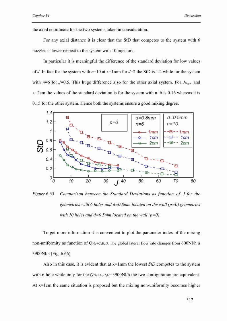
Capther VI Discussion
312
the axial coordinate for the two systems taken in consideration.
For any axial distance it is clear that the StD that competes to the system with 6
nozzles is lower respect to the system with 10 injectors.
In particular it is meaningful the difference of the standard deviation for low values
of J. In fact for the system with n=10 at x=1mm for J=2 the StD is 1.2 while for the system
with n=6 for J=0.5. This huge difference also for the other axial system. For JHopt. and
x=2cm the values of the standard deviation is for the system with n=6 is 0.16 whereas it is
0.15 for the other system. Hence both the systems ensure a good mixing degree.
Figure 6.65 Comparison between the Standard Deviations as function of J for the
geometries with 6 holes and d=0.8mm located on the wall (p=0) geometries
with 10 holes and d=0.5mm located on the wall (p=0).
To get more information it is convenient to plot the parameter index of the mixing
non-uniformity as function of QHe+C3H6O. The global lateral flow rate changes from 600Nl/h a
3900Nl/h (Fig. 6.66).
Also in this case, it is evident that at x=1mm the lowest StD competes to the system
with 6 hole while only for the QHe+C3H6O=3900Nl/h the two configuration are equivalent.
At x=1cm the same situation is proposed but the mixing non-uniformity becomes higher

Capther VI Discussion
313
for the system with n=6 respect to the system with n=10 for QHe+C3H6O>2700Nl/h. At
x=2cm this switch is realized for QHe+C3H6O>2500Nl/h.
It is worth noting again that for very low value of the lateral flow rate it is the system
with 6 holes to provide for the best mixing. In fact the biggest difference between the
mixing of the two systems are reached for QHe+C3H6O<2500Nl/h for x=1mm and 1 cm. For
x=2cm the StD are not so different.
Figure 6.66 Comparison between the Standard Deviations as function of QHe+C3H6O of
for the geometries with 6 holes and d=0.8mm located on the wall (p=0)
geometries with 10 holes and d=0.5mm located on the wall (p=0).
The comparison between the two configurations can be done also on the basis of the
diameter D of the inner zone where a low or no fluorescence signal is visible.
Fig.6.67 shows how the parameter D changes as function of J on curves parametric
in the axial distance. In fig 6.68 D is plotted as function of the lateral flow rate. In both the
cases it is possible to see that the internal zone dimension decreases more slowly in the
system with 10 holes respect to the system with 6 holes.
In general the more the number of jets, the lower the jets penetration is but the more
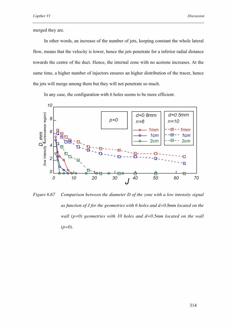
Capther VI Discussion
314
merged they are.
In other words, an increase of the number of jets, keeping constant the whole lateral
flow, means that the velocity is lower, hence the jets penetrate for a inferior radial distance
towards the centre of the duct. Hence, the internal zone with no acetone increases. At the
same time, a higher number of injectors ensures an higher distribution of the tracer, hence
the jets will merge among them but they will not penetrate so much.
In any case, the configuration with 6 holes seems to be more efficient.
Figure 6.67 Comparison between the diameter D of the zone with a low intensity signal
as function of J for the geometries with 6 holes and d=0.8mm located on the
wall (p=0) geometries with 10 holes and d=0.5mm located on the wall
(p=0).

Capther VI Discussion
315
Figure 6.68 Comparison between the diameter D of the zone with a low intensity signal
as function of QHe+C3H6O for the geometries with 6 holes and d=0.8mm
located on the wall (p=0) geometries with 10 holes and d=0.5mm located
on the wall (p=0).
Comparison between the geometries with 6 injector with a diameter equal to 0.8
mm and 0.9 mm located on the wall of the cylindrical duct
The comparison between the mixing efficiency of the systems with 6 injector with a
diameter equal to 0.8 mm and 0.9 mm located on the wall of the cylindrical duct has been
performed on the basis of the standard deviation of the normalized fluorescence intensity
profiles along a diameter of the cross sections located at x=1mm, 1cm and 2cm. The StD
has been plotted both as function of the momentum of the jet to the main flow stream J and
of the helium and acetone flow rate (QHe+C3H6O). In fact, since the global lateral flow is the
same but the dimension of the injectors are different, the velocities of the jets, as well as
the momentum of the jet to the main flow stream J, will be different. Hence, to compare the
results on the basis of the same axial coordinate the StD has been plotted also as function

Capther VI Discussion
316
of QHe+C3H6O.
For both the system the JHopt. is equal to 11.
Figure 6.69 Comparison between the Standard Deviations as function of J for the
geometries with 6 holes and d=0.8mm d=0.9mm located on the wall
(p=0)of the cylindrical duct.
Fig. 6.69.shows the mixing non-uniformity as function of the momentum of the jet to
the main flow stream J on parametric curves in the axial position. The dashed line are
relative to the configuration with 6 holes with an inner diameter equal to 0.9mm, while the
continuous lines are relative to the system with the same number nozzles but with an inner
diameter equal to 0.8mm.
For J=JHopt.=11 and x=2cm the systems seem to be equivalent.
Fig 6.70 shows the mixing non-uniformity as function of the helium and acetone
flow rate QHe+C3H6O. It is worthwhile noting that for x=1mm, x=1cm and x=2cm the StD
for the system with d=0.9 mm is always higher than the ones relative to the other system,
even if this difference is not so relevant. In fact, the values of the StD slightly differ from
each other for a fixed axial position and for a fixed value of the lateral flow rate QHe+C3H6O.
At x=2cm for the system with d=0.9mm the Standard Deviation (StD) is lower than

Capther VI Discussion
317
0.2 from QHe+C3H6O>1500Nl/h, while for the other system from QHe+C3H6O.>2200Nl/h.
Figure 6.70 Comparison between the Standard Deviations as function of QHe+C3H6O
of for the geometries with 6 holes and d=0.8mm d=0.9mm located on the
wall (p=0)of the cylindrical duct.
A further paragon between the two chosen configurations can be realized considering
the diameter D of the inner zone where a low or no fluorescence signal is detectable. In fig
6.71 D is plotted as function of the lateral flow rate.
In is possible to note that to the configuration with injectors with an inner diameter
(ID) equal to 0.9mm competes the highest values of the parameter D .
In particular at x=1mm, the zone where the fluorescence intensity is very low
disappears for QHe+C3H6O=2500Nl/min for the system with an inner diameter equal to 0.9,
while in the other system the same condition is respected for QHe+C3H6O=1800Nl/h.

Capther VI Discussion
318
Figure 6.71 Comparison between the diameter D of the zone with a low intensity signal
as function of QHe+C3H6O for the geometries with 6 holes with d=0.8mm and
d=0.9mm located on the wall (p=0)of the cylindrical duct.
Therefore, the configuration with an inner diameter equal to 0.8mm results to
provide for a better mixing in comparison with the configuration with holes with an inner
diameter equal to 0.9mm. As matter of fact, the jet velocity that competes to the former
system is higher since the dimension of the nozzles is smaller. This results in an higher
values of J and in a better penetration. Thus the jets penetrate further in the main duct and
allows the tracer to be spread out on all the cross section, whereas in the configuration with
diameters of 0.9mm, the jets penetrate for a smaller distance towards the central of the duct
respect to the other case considered, and there forms a wider central region where acetone
does not concentrate.
This leads to an increase of the non-uniformity of the mixing.
The numerical results were compared on the basis of the standard deviations of the
acetone concentration profiles along a diameter of the duct at several cross section for any
configuration considered in the numerical integrations. Comparisons are presented in the

Capther VI Discussion
319
next paragraph.
Comparison between the configuration with 6 and 10 injectors located on the
wall of the cylinder duct
The aim in this paragraph is to compare the geometries analyzed. In particular the
configurations with 6 and 10 injectors, located on the wall of the cylindrical duct with no
protrusion, have been considered. Before performing this analysis, it is important to
underline than the main flow and the lateral flow, injected by the nozzles inside the main
duct in the two systems considered, are the same. The different dimension and number of
injectors entail that the values of the momentum of the jet to man stream ratio J is
unequivocally different. Hence the comparison will be realized as function of parameter J
but also as function of the total lateral flow rate (QHe+C3H6O).
Fig. 6.72 show the mixing dis-uniformity as function of the parameter J, for the two
chosen .configurations, at different axial position from the convergent ( respectively
1mm,1cm and 2cm). It is possible to note that for any axial distance the value of the StD
that competes to the system with 6 holes is always lower respect to the geometry with 10
holes.
Fig. 6.73 show the mixing dis-uniformity as function of the parameter QHe+C3H6O, for
the two chosen configurations at different axial position from the convergent ( respectively
1mm,1cm and 2cm). The value of the parameter QHe+C3H6O goes from 1200Nl/h to
4000Nl/h. It is evident that the configuration with 6 hole ensure a best mixing respect to
the other geometry, in fact for any axial distance and for the most of the QHe+C3H6O values,
the value of the StD is lower in the first configuration.

Capther VI Discussion
320
.
Figure 6.72 Comparison between the Standard Deviation as function of the parameter J
at different axial position for the geometries with 10 and 6 injectors located
on the wall of the cylindrical duct
Figure 6.73 Comparison between the Standard Deviation as function of the lateral total
flow rate QHe+C3H6O at different axial position for the geometries with 6 and
10 injectors located on the wall of the cylindrical duct
Comparison between the configuration with 6 injectors located on the wall of the
cylinder duct and the configuration with 6 holes and a protrusion inside the cylinder duct

Capther VI Discussion
321
equal to1 mm.
The comparison between the configuration with 6 injectors located on the wall of the
cylinder duct and the configuration with 6 holes and a protrusion inside the cylinder duct
equal to1 mm is reported in fig.4.5.12.
The mixing dis-uniformity is reported as function of the parameter J, for the two
chosen configurations, at different axial position from the convergent (respectively 1mm,
1cm and 2cm).
Since in this case the number and dimension of holes is the same there is no need to
have two different diagrams. In fact the values of the parameters J and QHe+C3H6O are the
same in the two analyzed configuration.
In fig.6.73 it is possible to note that the values of the StD are very different. The
trend of the mixing disuniformity is always decrescent as function of J for any axial
distance from the convergent for the system with no protrusion. The other configuration
shows a minimum value of the mixing disuniformity for J=9 than it starts increasing
For any axial distance and for J from 3.5 to 11 the configuration with the protrusion
inside the duct allows for a best mixing of the different species. For J>11 the same
configuration does not provide for the best solution. For instance, for J=13 and x=1 cm the
value of the StD is higher in the case of the 6 injector protruded inside the duct. At x=1cm
and x=1mm this inversion is detectable for J=16 and 19.
The worsening of the mixing for high J becomes evident at J equal to about 25 where
the value of the StD in the case of the system with the protrusion at the axial coordinate
x=1 cm becomes equal to StD without protrusion but at an axial distance from the
convergent equal to 1mm.

Capther VI Discussion
322
Figure 6.73 Comparison between the Standard Deviation as function of the parameter J
at different axial position for the geometries with 6 injectors located on the
wall of the cylindrical duct and 6 injectors protruded inside the cylindrical
duct of 1mm.
Therefore, the geometry with 6 holes and a protrusion inside the main duct of 1 mm
results to provide a better mixing for low values of J in comparison with the other
geometry. In fact the protrusion of injectors inside the duct leads the jets to penetrate
further towards the center of the duct. Hence for low values of J , it results in an
improvement of the mixing. On the contrary when the values of J are enough high to
guarantee a good penetration of the jets, the protrusion causes on over-penetration of the
jet, hence they tend to form a central core and the acetone is accumulated in this region. It
causes and increase of the StD value and hence a worsening of the mixing.
Anyway these results suggest that the radial position of injection tubes is an
important parameter in order to achieve an efficient mixing of reactants for experiment in
the tubular reactor.

Capther VI Discussion
323
Discussion
Both the experiments and the numerical simulations clearly indicates that the best
mixing is reached in the case of six holes with a inner diameter equal to 0.8. In fact the StD
reaches a value lower than 0.15 earlier than the other configurations. The analyses anyway
show that an important parameter to shorten the mixing time is the position of tube inside
the main duct.
Therefore the mixing configuration and the reactor have been dimensioned.
The reactor that will be used at high temperature has been designed and realized.
It is shown in Fig.6.74. The first part is the mixing section. Six round, equally spaced,
holes are displaced on the perimeter of the first cylindrical duct at a radius distance to
the convergent. They house alumina tubes for lateral injection with an inner diameter
equal to orifice diameter computed from JHopt., sizable on request. The reactor is divided
into ten modules. A 10 cm sapphire tube and an alumina disk form each module.
Adjacent modules will be connected by two alumina threaded rods and bolts. Disks are
provided of an admission in order to allow for species or temperature sampling. In order
to avoid possible leakages a special ceramic sealer with a high content of alumina will
be used. Sapphire has been also chosen because of its high transparency in the visible
and ultraviolet wavelength range. The chosen materials are alumina and sapphire for
their physic properties: high thermal resistance, low conductibility and low thermal
expansion coefficient, inert and resistant in oxidant environment. Unfortunately alumina
is fragile, hard and not easily machinable. Alumina is used for the injection part,
threaded rods and disks.
These properties should allow the exploitation of elastic and anelastic light

Capther VI Discussion
324
scattering diagnostic techniques. These techniques are the most effective diagnostic
tools for the non-intrusive, space and time resolved characterization of the combustion
processes. The transparency of the reactor will also allow temperature profiles
measurement along the reactor by means of a thermograph camera.
Figiure 6.74 Reactor and mixing section.

Conclusion
325
CONCLUSIONS
The thesis has concerned the study of the behavior of model reactors in working
conditions typical of a Mild Combustion process and has given a fundamental contribution
for the comprehension of the oxidation process of small paraffins in “mild” operative
conditions and also for the resolution of problems correlated to the difficulty to set-up a lab
scale facility able to work with high inlet temperatures typical of the Mild combustion.
This new combustion “mode” forecasts the use of a high dilution degrees and a high pre-
hating of reactants. These operative conditions are very promising in the framework of the
development of new combustion technologies aimed to enhance the efficiency and reduce
the environmental impact of combustion systems. In fact they allow for a reducing of
pollutants formation and save energy.
The first step has been the identification of model reactors that can allow for an
accurate and exhaustive analysis of the chemistry and the dynamic evolution of the
combustion process. The choice has fallen on the continuous stirred reactor (CSTR) and on
and the plug flow configurations. Both reactors allow for studying the evolution of the
oxidation process as a succession of steady states as function of an unique parameter,
which is in the case of the CSTR, the time and, in the case of the plug flow reactor the
axial coordinate, or equivalently the time.
In literature there is not a consistent number of works on Mild processes in tubular
flow reactors since the very high inlet temperatures imply very strict requirements on the
materials to employ and on the efficiency of mixing devices. As matter of facts diluent and
comburent have to be fed separately from the fuel in order to avoid undesired reactions in
the pre-mixing section. At the same time they have to mix in a time relatively short in
comparison with the ignition time of any mixtures that forms during the mixing process.

Conclusion
326
This constrain is very severe because the very high inlet temperatures enhance the
oxidation reaction rates.
All these problems have properly faced, thus the contribution of this thesis to Mild
combustion studies has been the designing and the setting up a tubular flow reactor that
will be employed to characterize the Mild combustion as clean and cleaning technology.
The design of the tubular reactor has been realized by means of the classical
equations of a plug flow reactor. Several parameters have been fixed in order to achieve a
high-resolution time of the oxidation process, i.e. the residence time, and to satisfy safety
(power plant) and space (axial length of the reactor) requirements. The dimensioning of the
reactor responds to the requirement of achieving a full-developed motion of the fluid inside
the reactor, in order to avoid velocity, temperature and species concentrations gradients in
the radial coordinate of the system. In fact this condition guarantees that the evolution of
the oxidation process can be easily studied as function of the axial coordinate of the
reactor. From analytical calculations and the use of a computational commercial fluid-
dynamic code (Fluent), with the aim to characterize the fluid-dynamic field, all the
geometric parameters of the reactor have been assessed.
Furthermore the configuration has been designed in view of optical diagnostic
analyses, species samplings and temperature measurements, in order to characterize the
evolution of the oxidation process in terms of species production and concentration and
temperature trend along the axial coordinate of the reactor. The reactor in fact has a
modular structure. A 10-cm sapphire tube and an alumina disk form each module. Disks
are provided of an admission in order to have species or temperature samplings and the
sapphire will allow for optical diagnostic analyses.
The second step has concerned the choice and the dimensioning of the mixing
section of reactants.

Conclusion
327
The selection of the mixing configuration has derived from a thorough study of
mixing devices used in combustion systems. Mixing is realized with jets in cross flow
configuration. Fuel is hence injected inside the main duct trough nozzles orthogonal to the
directions of the main flow, which is composed by diluent and comburent at high
temperature. The mixing efficiency has been evaluated as function of the parameters
characteristic of this configuration by means of numerical simulations, using a
computational fluid-dynamic commercial code (Fluent software) and experimental tests
based on fluorescence measurements on a simplified configuration working at room
temperature. Several geometries have been tested and finally the mixing section has been
designed. The tubular reactor, the mixing section and the whole plant have been realized.
In the case of the CSTR configuration, it has been possible to carry out a thorough
experimental campaign since the reactor and the plant were already present in a laboratory
of the institute. Firstly the experimental facility has been modified in dependence of our
needs and all the problems, related to the choice of the reactor, i.e. the mixing, and to the
operative Mild conditions, i.e. high temperatures, have been faced. The experimental tests
were realized to characterize the combustion regimes that establish during the oxidation of
the system CH4/O2 diluted with nitrogen up to 90% as function of inlet temperatures and of
the mixture compositions. The framework outlined by the experimental analyses
underlines that extreme working conditions very different from the ones used in traditional
combustion processes, can lead to a very complex system behavior. Several thermo-kinetic
regimes corresponding to static and dynamic conditions were recognized. The efforts have
been hence focused on the characterization of the new behavior. As matter of fact
oscillations have been detected for paraffins with high molecular weights, but this is the
first time they have been experimentally recognized for methane. Hence an accurate
characterization of the dynamic region has been performed and several temperature

Conclusion
328
oscillation typologies have been identified. Results have been reassumed in a stability or
ignition map (C/O feed ratio-Tinlet). On this plane it has been clearly identified a region
where oscillation take place. The dynamic region extends for mixtures with a
carbon/oxygen feed ratio lower than twice the stoichiometric ratio and for inlet
temperatures comprised between 1050K and 1275K. Experimental tests has put in result
another meaningful behavior of the system in discussions, in fact for high feed ratios,
outside the dynamic region, and for inlet temperatures higher than 1175K a decrease of the
reactivity of the system has been detected. In fact the reactor temperature increase was
relatively low and assumed a constant value for further inlet temperatures increase.
The dynamic behavior and the exothermicity damping of the system have been
investigated as function of the main parameters of the systems, i.e. residence time, and
dilution degree of the system. They affect sensibly the insurgence of the dynamic behavior,
in fact a decrease of the dilution decrease and an increase of the residence time imply a
reduction of the extension of the dynamic region and an anticipation of the temperature
decrease towards lower temperatures. Further experimental analyses have been performed
in order to assess the effect of hydrogen addiction and of the nature of the diluent on the
dynamic behavior. It has been shown that hydrogen oxidation kinetic significantly interacts
with methane Mild Combustion process, in fact hydrogen addition decreases the
characteristic kinetic times of the system and reduces the zone where dynamic behaviors
occur, furthermore it provokes a shift of the reduction of the reactivity of the system
towards lower inlet temperatures. Results suggest that the system is very sensible to the
presence of hydrogen but not to its relative concentration. It implies that just small amount
of hydrogen can be added to the system to influence the insurgence of oscillations. Similar
effects have been achieved whether part of the diluent is substituted with steam water,
while keeping constant the overall dilution degree. The results show that the reactivity of

Conclusion
329
the system slightly increases for low temperatures and the exothermicity of the system
damps for lower temperatures respect to the system completely diluted in nitrogen.
Furthermore steam water limits the insurgence of oscillations for rich mixtures and high
temperatures. Numerical simulations have then shown that steam water interacts with the
methane oxidation mechanism-giving rise to breakdown reactions thus enhancing the
radical amount and the reactivity of the system.
From the study on the evolution of the dynamic phenomenology as function of the
parameters of the system appear clear a common trend: the decreases of the dilution level,
the decrease of the residence time, the hydrogen addiction and the dilution in steam water
act enhancing thermally or kinetically the reactivity of the system inducing a reduction of
the extension of the dynamic region and a shifts towards lower inlet temperature of the
exothermicity damping recognized for high temperatures and rich mixtures in the stable
combustion region.
The availability of kinetic oxidation mechanisms has suggested the possibility to go
deep inside this new phenomenology by means of numerical simulations. Firstly it has
been verified whether models were able to reproduce of the dynamic behavior detected
experimentally. At the light of the good results obtained, kinetic models have been used to
perform further simulations in order to understand what are the reactions responsible of the
insurgence of the dynamic phenomenology and the exothermicity-damping of the system.
On the basis of comparison between experimental (C2 species gas chromatographic
samplings) and numerical results (species rate of production analysis) it has been supposed
that the dynamical behavior evidenced during methane oxidation is due to the interaction
between the kinetic of the methane oxidation and the thermal exchange between the reactor
and the environment. Although the chain branching of the CH4 reaction mechanism is
basically due to the H2/O2 system, methane evolves according two main pathways that are

Conclusion
330
the oxidation and the recombination channels respectively. The rate of production analysis
showed that recombination channel acts subtracting CH3 radicals from the oxidation
channel, storing them as C(2) compounds. In particular ethane can be dehydrogenated until
the formation of the vinyl radical (C2H3). It can be further dehydrogenated to acetylene or
oxidized to acetaldehyde.
When the chain branching starts, the recombination channel releases the CH3 radicals
through the formation of acetaldehyde and its dehydrogenation until the formation of
CH3CO radicals. These, in turn, are thermally decomposed, producing CH3 radicals and
CO that feed the oxidation channel enhancing the reactivity of the system and causing the
temperature increase. If the recombination channel releases these radicals the system can
evolve through an oscillation regime whereas if it stores them as C2H2, the system evolves
through a stable combustion regime characterized by a very low temperature increase.
Therefore, oscillations occur as result of the competition between the oxidation and
recombination channels present in the kinetic mechanism of methane combustion while the
exothermicity damping is linked to the prevalence of acetylene formation and its
stabilization with respect to the oxidation of the recombination products with two carbon
atoms when the rich mixture temperature is higher than a threshold value.
Therefore Mild Combustion conditions have been shown to significantly influence
the fuel oxidation kinetic. The very high initial temperature and the very low concentration
of reactants strongly modify the competitions among the different kinetic pathways thus
stressing behavior that are usually hidden in traditional combustion conditions by very fast
oxidation process both for high and low molecular weight hydrocarbons.
The information content of static and dynamic behavior can be useful to better
understand the oxidation kinetic of small paraffins and to verify the effectiveness of kinetic
models available in literature, focusing the attention to oscillation phenomenology and the

Conclusion
331
occurrence of the different thermo-kinetic regimes. In fact this experimental evidence
represents a rigorous test for validation of kinetic models that must be able to predict the
dynamic behaviors of reacting system, thus considering more stringent constraints.
From a practical point of view, the presence of such oscillatory regimes, due to
thermo-kinetic behavior of the system, could induce a negative phenomenology. In fact,
their coupling with physical processes could give rise to high frequency oscillations in
combustion chambers, generally responsible of efficiency decrease and of serious damages
in gas turbine burners. Such dynamic behavior is hidden in conventional processes
involving methane by the relatively fast oxidation kinetic that characterizes traditional
gaseous fossil fuels. Moreover, the activation of different kinetic pathways hypothetically
responsible of oscillations could induce an increase of pollutant formation.
The results hence help to identify the operative condition in which a Mild
Combustion process should be realized. The experimental results unambiguously show that
the instability problems can be overcome by splitting the whole combustion process in two
stages where the first one evolves in diluted rich conditions, i.e. C/O ratio where no
oscillations were detected and second stage completes the oxidation process.
An alternative way to avoid these phenomenologies concerns the use of additive fuel
that can act on oxidation kinetic improving the evolution of the system towards a static
steady state. To this aim results suggest acting on the mixture composition or on the
diluent. In fact small addiction of hydrogen to the system or the dilution of the system in
steam water allows working with steady combustion for a larger number of operative
conditions. Furthermore the highest reactivity induced by the presence of hydrogen
suggests the possibility of using small amount of this clean fuel whether Mild combustion
process has to be realized with low calorific power and less valuable fuels than methane.


APPENDIX

APPENDIX
1
6 injectors with d=0.9mm located on the wall of the cylindrical duct
The second analyzed geometry presents 6 injectors with an inner diameter equal
to 0.9 mm. They are equally displaced on the perimeter of the cylindrical duct at 60°
of distance from each other.
In this case the optimal value of the momentum of the jet to main stream ratio J
according to Holdeman equations is equal to 11 (JHopt.). The numerical simulations
have been run for a wide range of J, from 0.5 to 17, in such a way it has been possible
to analyzing the mixing in a wide range of conditions. If fact the analyses have been
realized for J values lower and higher than the JHopt..
The bi-dimensional implementation of the fluorescence measurements
performed for this configuration is presented in figure 1.
The acetone distribution inside the system is represented by the intensity of the
pixel of images collected by means of the optical diagnostic facility well described in
the first paragraph.
The fluorescence intensity has been divided into 16 levels and colors, and the
values have been normalized in comparison to the highest intensity value of all the
images collected for the several configurations considered, in order to compare all the
experimental results among them. The normalized pixel intensity values go from 0 to
1800.The images have been collected for three different cross sections located in the
plane x=0 and at an axial distance equal to x=1mm, x=1cm and x=2cm. In the figure it
is also reported the laser beam that hits the cylindrical duct. The figure allows the
analysis of the acetone distribution as function of the parameter J, once the axial
position has been fixed, as well as the analysis of the acetone distribution as function
of the axial position, if the value of the parameter J has been fixed.

APPENDIX
2
Figure 1 Fluorescence Intensity images as function of the parameter J in curvesparametric on the axial position for the configuration with 6 holes witha inner diameter equal to 0.9 mm positioned on the wall of thecylindrical duct.

APPENDIX
3
At the axial position equal to 1mm and for values of J from 0.5 to 6, there is a
wide region where a low or no fluorescence signal is detectable. Acetone mainly
accumulate in the near-wall region. For J=8 the intensity fluorescence begins to be
consistent but the signal is not uniform. The same consideration applies for J=11 and
J=14. For a value of the parameter J equal to 17 the signals appears more uniform in
all the points of the cross section.
In section located at x=1cm the internal region with a concentration of acetone
close to zero tends to fade as J is increased from 0.5 to 3 and it completely disappears
for J equal to 4. from J=4 to J=11 the intensity signal is increasingly higher in the
central region but the signal becomes uniform for J=14.
In the cross section located at x=2cm, for J comprised between 0.5 and 2, the
region where the intensity signal is not detectable is still present but it diminishes and
disappears for J=3. For J=4 and 5 intensity I the center of the cross section increases
and the signal seems to be uniform for J=6. For J>6 the tracer is spread out on all the
surface and a good mixing degree is reached.
It is also possible to analyze the trend of the uniformity of the signal as function
of the axial distance from the convergent once the parameter J is fixed.
For J=0.5, 1 and 2, at x=1mm the fluorescence signal comes from the near-wall
region but in the center of the cross section the white color suggests the complete
absence of acetone. As the axial distance increase the only difference is that the white
region extension reduces.
For J=3 and at x=1mm and 1cm the region with no signal is still present but at
x=2cm the acetone begins to spread out towards th center of the duct.
For J=4 and J=5 for x=1mm the acetone has a relatively low concentration in
the center of the cross section but it accumulates in the near-wall region. For x=1cm

APPENDIX
4
and 2cm the acetone spreads toward the internal area ut its concentration is still lower
in comparison with the surroundings.
For J=6 and x=1mm a low concentration nucleus is still evident but it fades for
x=1cm and the situation improves at x=2cm where the signal begins to be more
uniform.
For J=8 and J=11 at x=1mm the acetone is present in all the area but it is not
homogeneously distributed. The distribution improves at x=1cm and at x=2cm the
tracer is uniformly spread out.
For J=14 and J=17 the segregated zone with a low signal is very narrow and for
the other two axial position the acetone is well distributed in the whole cross section.
In fig.2 the fluorescence intensity signal is plotted along a diameter of the duct
at the known axial distances for any J value analyzed.
In these figures the fluorescence intensity has been normalized respect to its
mean value for each working condition. In such a way the profiles have been made
independent on the acetone concentration and they can be reasonably compared
among them.
The same analyses and considerations can be realized taking into account the
normalized fluorescence profiles reported in figure 2. In this case the uniformity of
acetone distribution is reached when profiles becomes flat.
For J=0.5 and J=1 it is evident that the jets do not penetrate sufficiently in the
first section of the simplified configuration and the tracer tends to accumulate in the
region close to the wall of the third section of the system.
For value of J>8 the fluorescence intensity profiles at x=1cm and x=2cm almost
coincide.

APPENDIX
5
Figure2 Fluorescence Intensity signal profiles as function of the parameter J incurves parametric on the axial position for the configuration with 6holes with a inner diameter equal to 0.9 mm positioned on the wall ofthe cylindrical duct.

APPENDIX
6
In fig.3 the non-uniformity of the mixing, calculated on the basis of the standard
deviation, is presented as function of the parameter J on curves parametric on the axial
position. The StD has been calculated considering the normalized pixel fluorescence
intensity values presented in fig. 2.
The higher the momentum of the jet to mainstream ratio, the lower the StD is for
any axial distance. As matter of fact, the StD decreases monotonically as the
parameter J is increased. For x=2cm it mainly diminishes from J=0.5 to J=6, than for
all the axial distances it seems to reach a constant value. At x=1mm the StD goes from
0.9 to 0.21, while for x=1cm it goes from values very close to 78 to 0.16, and for
x=2cm it interests J values from 0.68 to 0.14.
The StD is never lower than 0.1 but for x=2cm is lower than 0.2 for J>6. For
x=1cm it is lower than 0.2 for J>14 while at x=1mm it always higher than this value.
Figure 3 Standard Deviation of the fluorescence intensity signal along adiameter of the duct as function of the parameter J on curvesparametric in the axial position.
6 injectors with d=0.8 mm located on the wall of the cylindrical duct
The third analyzed configuration has 6 injectors with an inner diameter equal to
0.8 mm. They are equally displaced on the perimeter of the first cylindrical duct at 60°
of distance from each other.

APPENDIX
7
Also in this case, the optimal value of the momentum of the jet to main stream
ratio J according to Holdeman equations is equal to 11 (JHopt.). The numerical
simulations have been run for a wide range of J, from 1 to 34. These values change in
comparison with the configuration considered in the previous paragraph since,
although the lateral flow rate is the same, the velocity of the lateral jets increases
because of the cross section of the injectors is smaller. It means that the numerator of
the J formula is higher respect to the one that competes to the geometry with the same
number of holes but with an inner diameter equal to 0.9 mm. Anyway also in this
case, the mixing efficiency has been studied in a significant range of working
conditions. As matter of fact, the analyses have been realized for J values lower and
higher than the JHopt..
The figure 4 shows the bi-dimensional implementation of the fluorescence
measurements realized for this configuration. The fluorescence intensity signal is
reported in the three cross sections located at an axial position equal to 1mm, 1cm and
2 cm as function of the momentum of the jet to main stream ratio J.
The images allow the analysis of the acetone distribution as function of the
parameter J, once the axial position has been fixed, and the analysis of the acetone
distribution as function of the axial position, one time the value of the parameter J has
been fixed. The fluorescence intensity has been divided into 16 levels and colors, and
the values have been normalized in comparison to the highest intensity value of all the
images collected for the several configurations considered, in order to compare all the
experimental results among them. Also in this case the normalized pixel intensity
values range from 0 to 1800. At x=1mm from J=1 to J=7 there is a small central area
where the fluorescence signal is very weak but as J increases the extension of this area
is significantly reduced.

APPENDIX
8
Figure 4 Fluorescence Intensity images as function of the parameter J in curvesparametric on the axial position for the configuration with 6 holes witha inner diameter equal to 0.8 mm positioned on the wall of thecylindrical duct.

APPENDIX
9
The acetone concentrates in the near-wall region. For J=9 the tracer spreads out
towards the center of the cross section but there is still a significant gradient of
concentration along a radius of the duct.
The gradient of the acetone concentration diminishes as J increases and for J=34
it is very close to zero. In other words, the acetone distribution seems to be almost
homogeneous.
At x=1cm, from J=1 up to 5, the images clearly show an internal region where
the fluorescence signal is very low. Once again the acetone accumulates in the
periphery of the cross section. From J=7 a J=11 the acetone from the near-wall region
goes towards the center of the cross section and from J=16 to J=34 the mixing appears
to be uniform.
In the last cross section considered, for J=1 and 2 there still exists a central zone
where the signal is very low but it disappears for J=3. For J=5 the acetone
concentration is lower in comparison with the surrounding area but for J>7 the signal
becomes uniform. Hence it is possible to assume that the system has reached a good
nixing degree. The second analysis leads to similar r results. It consists in the
discussion of the mixing uniformity trend as function of the axial position once the
parameter J is mixed. For J=1 and J=2 the images in all the three axial positions show
that the signal is relatively low in the center of the duct but it is concentrated in the
near-wall region. The extension of this area tends to reduce but it does not disappear
as the axial position is moved from 1mm to 2 cm. For J=2, 3 and 5 the situation is the
same except for the axial distance equal to 2cm where the jets sufficiently penetrate
inside the main duct to ensure a significant presence of acetone also in the central
region. The system reaches a uniformity in the fluorescence signal at x=2cm for a
value of the parameter J equal to 7.

APPENDIX
10
Figure 5 Fluorescence Intensity signal profiles as function of the parameter J incurves parametric on the axial position for the configuration with 6holes with a inner diameter equal to 0.8 mm positioned on the wall ofthe cylindrical duct.
From J=9 the central zone with a low fluorescence signal is very small, it is

APPENDIX
11
smaller at x=1cm and it fades at x=2cm. From J=16 up to 34 the system presents a
good mixing degree for x=1cm and for x=2cm the images seem to be very similar
among them. In any case, at this axial distance, the acetone distribution appears to be
uniform.
The results, obtained considering the fluorescence intensity images collected at
different axial positions from the convergent, can be done also taking into account the
profiles of fluorescence intensity along a diameter of the three cross sections at
x=1mm, x=1cm and x=2cm. The profiles are shown in fig.5. In these figures the
fluorescence intensity has been normalized respect to its mean value for each axial
position and J. In such a way profiles have been made independent on the acetone
concentration and they can be reasonably compared among them. The unit of
fluorescence intensity is arbitrary.
Figure 6 Standard Deviation of the fluorescence intensity signal along adiameter of the duct as function of the parameter J on curvesparametric in the axial position.
For J=1 and J=2, it is evident that the jet penetration is low in fact the
normalized intensity profile is high in the near-wall region but zero in the center for
x=1mm and x=1cm. For x=2cm it grows and becomes equal to 0,4. From J>16 the
profile at x=1cm and 2 cm are similar. For J=34 all the fluorescence signal values

APPENDIX
12
seem to coincide for any radial position.
In fig. 6 the non-uniformity of mixing is plotted as function of the J value at the
three axial distance x=1mm, x=1cm and x=2cm. The standard deviation is calculated
on the basis of the normalized fluorescence profile reported in figure 5.3.8.
For x=1cm the StD becomes lower than 0.2 for J=16, while for x=2cm for J=7.
For this axial distance it reaches the minimum value for J=11 and than it is constant
for higher value of J. For x=1mm the lowest value is 0.26 and it competes to the
highest value of J here analyzed.
6 injectors with d=0.9 mm protruded 1mm inside the cylindrical duct
The fourth analyzed geometry has 6 injectors with an inner diameter equal to 0.9
mm. They are equally displaced on the perimeter of the cylindrical duct at 60° of
distance from each other. This configuration has already been analyzed in the
paragraph 5.3.b but in this case the injectors are protruded 1mm inside the main duct
(p=1mm). The optimal value of the momentum of the jet to main stream ratio J,
according to Holdeman equations, is equal to 11 (JHopt.). The numerical simulations
have been run for a wide range of J, from 0.5 to 17. Hence, the analyses have been
realized for J values both lower and higher than the JHopt.. The fig. 7 shows the bi-
dimensional implementation of the fluorescence measurements realized for this
configuration. As in the previous cases, the fluorescence intensity has been
normalized respect to the highest of the intensity signal of all the fluorescence
measurements realized and it has been subdivided in 16 levels. It goes from 0 to 1800.
The acetone concentration is considered to be significant from values of the
normalized fluorescence intensity higher than the fourth level hence higher than 450.

APPENDIX
13
Figure 7 Fluorescence Intensity images as function of the parameter J in curvesparametric on the axial position for the configuration with 6 holes withan inner diameter equal to 0.9mm protruded 1mm inside thecylindrical duct.
APPENDIX
14
The signal is shown as function of the radial position (x=1mm,1cm and 2cm)
and the momentum of the jet to main stream flow J.
At x=1mm from J=0.5 up to J=4 it is present a central nucleus where the
acetone concentration is lower than 450. Enhancing the lateral flow rate, hence the
parameter J, the area with a fluorescence signal lower than 450 reduces significantly
its extension. From J=0.5 up to J=2 it is possible to see the single jets since they do
not completely merge.
From J=5 there is a gradient of acetone from the near-wall region towards the
center of the cross section but it tends to zero as J increases. For J=14 and J=17 the
acetone concentration in the central area and in the near-wall area is equal but there
still exists a zone intermediate between the last two cited zones where the
concentration is higher.
From J comprised among 5 and 14 a new condition delineates. As matter of fact,
the signal is not detectable in the region very close to the wall of the duct. This is due
to the jets over-penetration in the main cylindrical duct. The tracer accumulates in the
region of the cross section between the central and the near-wall region.
At an axial distance from the convergent equal to 1cm, from J=0.5 to J=3 there
is a zone with a low fluorescence signal. For J=4 and J=5 the acetone spreads out
towards the central zone but there still exist a significant concentration gradient along
the radius of the duct. From J>5 the uniformity of the signal becomes increasingly
better.
At x=2cm and J=0.5 and 1 the signal is lower than 450 in the central zone. From
J=2 the signal is detectable in any point of the area of the cross section but it is not
uniform. From J>5 the mixing improves and the system reaches a good degree.
The second analysis concerns the study of the mixing uniformity as function of

APPENDIX
15
the axial position of the cross section of the second cylindrical duct, once J has been
fixed.
In the cross sections located at x=1mm and x=1cm for J from0.5 up to 3, there
exist a zone where the fluorescence intensity signal is lower than 450. This area is
located in the center of the duct and its extension reduces as the axial position changes
from 1mm to 1cm. At x=2cm, for J=0.5, 1 and 2 the acetone does not spread out
towards the center of the duct but the region where acetone is not present diminishes.
At x=2cm this region disappears but the signal is not uniform.
For J=4 and x=1mm the internal core with a low fluorescence signal is very
narrow but it disappears for x=1cm. For J=6 and x=1mm the signal is detectable for
any pixel of the image but it is not uniform in fact the acetone concentration in the
near-wall region is lower than the ones of the intermediate zone and of the center. The
uniformity condition is gained at x=1cm.
For J>6 the system reaches a good mixing degree even if it is evident at x=1mm
the jets over-penetrate and the tracer is not present in the region near the wall.
In fig. 8 it is shown the fluorescence intensity signal along a diameter of the duct
on the cross section at x=1mm, x=1cm and x=2cm. In these figures the fluorescence
intensity has been normalized respect to its mean value for each axial position and J.
In such a way profiles have been made independent on the acetone concentration and
they can be reasonably compared among them. The unit of fluorescence intensity is
arbitrary.
In any sequence of the fluorescence intensity profiles, it is worth noting that
there is an intermediate zone comprised between the near-wall region and the center
of the duct where the acetone concentration reaches its highest values.

APPENDIX
16
Figure 8 Fluorescence Intensity signal profiles as function of the parameter J incurves parametric on the axial position for the configuration with 6holes with a inner diameter equal to 0.9 mm protruded 1mm inside thecylindrical duct.

APPENDIX
17
It happens that when J is increased the signal becomes more and more uniform
in the center and in the middle section but not in the near-wall region. Also for J=17
the fluorescence gradient is zero in the middle and central area but not in the
surrounding area.
It happens that when J is increased the signal becomes more and more uniform
in the center and in the middle section but not in the near-wall region. Also for J=17
the fluorescence gradient is zero in the middle and central area but not in the
surrounding area.
Furthermore the concentration of the tracer in the near-wall region as J increases
becomes always lower. It depends on the too high jet penetration that does not allow
the tracer to spread out towards the lateral region.
The results, obtained considering the fluorescence intensity images collected at
different axial positions from the convergent, can be done also taking into account the
profiles of fluorescence intensity along a diameter of the three cross sections at
x=1mm, x=1cm and x=2cm. The profiles are shown in fig.9. In these figures the
fluorescence intensity has been normalized respect to its mean value for each axial
position and J. In such a way profiles have been made independent on the acetone
concentration and they can be reasonably compared among them. The unit of
fluorescence intensity is arbitrary.
In the case of x=1mm, the Standard deviation decreases monotonically but in at
x=1cm and x=2cm it presents a minimum value respectively for J=6 and J=3. As
matter of fact, the non-uniformity of the mixing increases after these values increase
and the StD is lower than 0.2 just for J=3.

APPENDIX
18
Figure 9 Standard Deviation of the fluorescence intensity signal along adiameter of the duct as function of the parameter J on curvesparametric in the axial position.
6 injectors with d=0.8 mm protruded 1mm inside the cylindrical duct
The last analyzed geometry has 6 injectors with an inner diameter equal to 0.8
mm. They are equally displaced on the perimeter of the cylindrical duct at 60° of
distance from each other. This configuration has already been analyzed but in this case
the injectors are protruded 1mm inside the main duct (p=1mm).
The study has been realized for a wide range of J, from J=4 to J=37, in such a
all the possible penetration (under- and over-penetration) conditions of jets are
represented.
The fig. 10 shows the bi-dimensional implementation of the fluorescence
measurements realized for this configuration. As in the previous cases, the
fluorescence intensity has been normalized respect to the highest of the intensity
signal of all the fluorescence measurements realized and it has been subdivided in 16
levels. It goes from 0 to 1800. The acetone concentration is considered to be
significant from values of the normalized fluorescence intensity higher than the fourth
level hence higher than 450.

APPENDIX
19
Figure 10 Fluorescence Intensity images as function of the parameter J in curvesparametric on the axial position for the configuration with 6 holes withan inner diameter equal to 0.8mm protruded 1mm inside thecylindrical duct.

APPENDIX
20
At x=1mm and for J=1 and J=2 there is a central area where any fluorescence
intensity signal is detectable. For J=3 up to J=9 the signal is not zero but anyway
lower than 450 in the central area while in it becomes increasingly higher in the
surrounding area. From J=11 the tracer spreads out towards the center of the system
and the fluorescence intensity signal becomes meaningful in any point of the cross
section From J=16 the intensity of the fluorescence signal from the center becomes
higher and higher and for J=34 it is reaches the highest values.
Likewise, at x=1cm from per J=1 up to J=3 the system there exists a zone where
the signal is low or zero, it fades completely for J=7 and the signal intensity is always
higher in the area comprised between the near-wall region and in the central area.
For J=11 the acetone is present in all the section almost uniformly but in the
near wall region. For J=21 and J=27 the system seems to be well-mixed but at J=35
the acetone concentration in the center zone reaches its highest values. In all these
conditions, it is visible that the jets over-penetrate in fact the acetone concentration in
the near-wall region is lower in comparison with points of the remaining region.
In the last cross section analyzed, located at x=2cm, from J=1 up to J=7 is still
visible a central core with a low acetone concentration but it becomes smaller and
smaller as J is increased. For J=9 it completely disappears and the fluorescence signal
suggests the system is well mixed. The situation improves for J>9 up to 27 where it
seems that the concentration in the central area becomes to high in comparison with e
surrounding area. Although the signal seems to be uniform the acetone does not
properly spread out towards the near wall region since the jets over-penetrate and
form a central core rich of acetone.
The second analysis concerns the study of the mixing uniformity as function of
the axial coordinate once the momentum of the jet to main stream ratio J has been

APPENDIX
21
fixed.
For J=1 at x=1mm it is visible a central core where no signal is measurable. This
situation persists for x=1cm and x=2cm. The same trend is clearly shown in the
sequence of images for J=2, 3, 5 and 7 as function of the axial coordinate.
For J=9 the situation slightly change, in fact at x=2cm the signal appears to be
almost uniform. For J=11 at x=1mm the acetone concentrates in the intermediate area
and it starts to significantly accumulate in the central region. At x=1cm the signal
become more uniform, in fact the signal relative to the central area has the same
intensity of the one coming from the intermediate area. At x=2cm the signal is
uniform but it is lower in the near-wall area respect to the remaining section. The
same situation is proposed for J=16 and 21 as function of the axial direction.
For J=27 the signal is sufficiently uniform in the central and intermediate region
but it is lower in the near-wall region at x=1mm, it slightly improves at x=1cm but at
x=2cm the central core becomes very high and there is a gradient from the center
towards the wall. For J=34 the acetone is always higher in the central region in
comparison with the remaining section for any value of x.
In fig.11 it is shown the fluorescence intensity signal along a diameter of the
duct on the cross section at x=1mm, x=1cm and x=2cm. In these figures the
fluorescence intensity has been normalized respect to its mean value for each axial
position and J. In such a way profiles have been made independent on the acetone
concentration and they can be reasonably compared among them. The unit of
fluorescence intensity is arbitrary. It is possible to get the same information analyzing
the intensity profiles as function of J or as function of x. In particular the jet over-
penetration causes the insurgence of an intermediate area where acetone concentrates.

APPENDIX
22
Figure 11 Fluorescence Intensity signal profiles as function of the parameter J incurves parametric on the axial position for the configuration with 6holes with a inner diameter equal to 0.8 mm protruded 1mm inside thecylindrical duct.

APPENDIX
23
For J>11 the profiles are more uniform and they almost coincide. It is possible
to note that the normalize intensity signals is always lower in the near-wall region
respect to the remaining region. In fig.12 it is shown the non-uniformity, hence the
standard deviation of the fluorescence signal along a diameter of the duct, in the cross
section located at x=1mm, 1cm and 2cm. For x=1mm the StD decreases
monotonically. It goes from 0.78 to 0.27. It firstly diminishes abruptly from J=1 to
J=11 and than it almost reaches a constant value. For x=1cm and x=2cm the standard
deviation first decreases and than slowly increases. In particular at x=1cm the
minimum StD value is reached for J=11, and at x=2cm for J=3. For x=1cm the StD
goes from 0.55 to 0.27, and for x=2cm it is 0.323 for J=1 and 0.27 for J=34.
From J=11 the StD values at x=1cm and x=2cm are very similar at any J value
and the for J=34 the system presents always the same non-uniformity distribution
degree. The system reaches an acceptable mixing for J comprised between 2 and 11
for x=2cm, while in the cross section located at x=1cm just for J=11, hence just in
these conditions the StD is lower that 0.2.
Figure 12 Standard Deviation of the fluorescence intensity signal along adiameter of the duct as function of the parameter J on curvesparametric in the axial position.


References
Allenby S., Chang W-C., Megaritis A., Wyszy ski M L., “Hydrogen enrichment: a way to maintaincombustion stability in a natural gas fuelled engine with exhaust gas recirculation, the potential offuel reforming” Proceedings of the I MECH E Part D Journal of Automobile Engineering 16 March2001, vol. 215, no. 3, pp. 405-418(14).
Ashwani K.Gupta “Flame characteristic and challenges with high temperature air combustion” 2nd
International Seminar on high temperature air combustion in industrial Furnaces January 17-18,2000 Stokholm, Sweden
Barbieri G., Di Maio.F.D, Lignola P.G and M. L. Loiacono “Modeling Methane Cool Flames andIgnition” Combust. Sci. and Tech., 1995 Vol. 106, pp.83-102
Bade Shrestha S.O., Karim G.A., “Hydrogen as an additive to methane for spark ignition engineapplications“, International Journal of Hydrogen Energy 24: 577-586.
Basevich.V.YA and Kogarko S.M. “The mechanism of methane combustion: cool-flame oxidation”Oxidation Communication 3, Nos 3-4, 199-2108(1983).
Beer J.M.” Clean combustion in gasin gas turbines: chellenge and technical responses”, Review J,Inst. Energy 68,2-10 (1995).
Brezinsky K., Burke E.J. and Glassman I. The high temperature oxidation of Butadiene TwentiehSymposium (International on Combustion/The Combustion Institute , 1984/pp. 613-622.
Brown, M.J and Parkins, N.D., 1991, Progress in the partial oxidation of methane to methanol andformaldehyde. Catal. Today,8:305-335.
Cavaliere A., de Joannon M. (1999) “Mild Combustion of High Temperature Reactants”, 2nd
International High Temperature Air Combustion” , Taiwan, January 20-22.
Cavaliere A., Lezioni di Combustione, ed.E.Albano,2000
CHEMKIN Collection, Release 3.7, Reaction Design, Inc., San Diego, CA (2000).
Chen C.J., Back M.K., and Back R.A, 1976. The thermal decomposition of methane II. Secondaryrections, autocatalysis and Carbon formation; non Arrhenius behaviour in the reaction of CH3 withethane. Ca.J. Chem. 54(20): 3175-3184.
Chen G., Spliethoff H., Yang L.B. Andries J. Hydrogen production from gasification-pyrolisis ofbiomass. III International Slovak Biomass Forum February 3rd-4th, 2003.
Cooper C. D., Calusen C.A., Tomlin D, Mike H and Martinetz A. “Enhancement of organic vapourincinerator using Hydrogen peroxide” Journal of Hazardous material, 27 (1991) 273-285.
Dagaut P. , Nicolle A. (2004) ”Experimental and detailed chemical kinetic modeling of hydrogen-enriched natural gas blend oxidation over extended temperature and equivalence ratio ranges”,Proceedings of the Combustion Insitute 30

Das L.M., Hydrogen-Oxygen Reaction Mechanism and its implication to hydrogen enginecombustion, Int. Journal of Hydrogen Energy vol.28 No. , pp. 703-715, 1996.
Dagaut P. , Nicolle A. (2004) ”Experimental and detailed chemical kinetic modeling of hydrogen-enriched natural gas blend oxidation over extended temperature and equivalence ratio ranges”,Proceedings of the Combustion Insitute 30
Denn M. Process Fluid Mechanics, Prentice-Hall, 1980.
de Joannon M., Langella G.,Beretta F., Cavaliere A., Noviello C. Proceedings of 5th InternationalConference on Technologies and Combustion for a Clean Environment, 435, Lisbon, July 12-15,July ,1999.
de Joannon M., Saponaro A., Cavaliere A. (2000) “Zero-dimensional analisis of methane dilutedoxidation in rich conditions” Proceedings of the Combustion Institute, vol.28 pp. 1639:1646.
Demetriades A., Yapuncich F.L. (1992) AIAA Journal 30:1795-1799.
Di Maio F.P., Lignola P.G. (1993) “Oscillations in CSTR Combustion Processes”, Joint Meeting ofthe Italian Section of the Combustion Institute, I.21, Rome, 3 -5 June.
Donley E., Lewandowsky, Optimized Design and Operating Parameters for Minimizing EmissionsDuring VOC Thermal Oxidation, Process CombustionCorp., Pittsburgh, 1996
Egret J. , Sochet L. et Lucquin M. (1965) “La combustion ménageé du methane à bassetempérature” Bull. Soc.Chim., 8, 2205.
Eklund H., Sundkvist S., Wilhelmsen K., Asen K.I., Griffin T. “Development of a membrane basedCO2 emission free Gas Turbine System”. Proceedings of Seventh International Conference onEnergy for a Clean Environment, 15.6, Lisbon, July 7-10 2003.
Feugier A., Influence of water vapor on hydrogen combustion National Bureau of Standards SpecialPublication 561, proceeding of the 10th Materials Research Symposium on Characterization of HighTemperature Vapors and Gases held at NBS, Gaitherburg, Maryland, September 18-22, 1978.
Forbes K.L. “Limit-cycle behaviour in a model chemical reaction:the Sal’nikovthermokineticoscillator” Proc.Roy.Soc.Lond. A(1990) 430, 641-651.
Fotache C.G. , Kreutz T.G. , Law C.K. (1997) “Ignition of hydrogen-enriched methane by heatedair”,Combustion and Flame 110: 429-440 .
Gray P., F.R.S., Griffiths J.F., Hasko S.M. and Lignola P.G. (1981) “Oscillatory ignition and coolflames accompanying the non-isothermal oxidation of acetaldehyde in a well stirred reactor”Proc.Roy.Soc.Lond. A 374, 313-339 .
Guéret , C. 1993. Valorisation du Methane en hydrocarbures superieurs: etude paramerique etModelecinetique. PhD thesis, Institute National Polytechnique de Lorraine.

Guéret et al, Daroux M. and Billaud F.1997 Methane pyrolysis: thermodynamics Chem. Eng.Science, 52 (5): 815-827.
Gupta A.K. Flame characteristic and challenhges with high temperature air combustion. 2nd
International Seminar on high temperature air combustion in industrial Furnaces, January 17-18,2000 Stockholm, Sweden.
Hang B., Sung C.J. Effects of vitiated air on hydrogen ignition in a supersonic laminar mixinglayer.
Hansen D.A.,Lee E.K. Radiative and non radiative transitions in the fristexited singlet state ofsimple linear aldehydes, J.Chem.Phys.,63/8, 3272-3277, 1975
Hashimoto T.,Combustion stability of a vitiated-air Heater using coaxial injectors, EnergyConvers Mgm Vol.38 , No 10-13
Hatch M.S., Sowa W.A., Samuelsen G.S. and Holdeman J.D. Jet Mixing Into a Heated Cross Flowin a Cylindrical Duct: Influence of Geometry and Flow Variations. Journal of Propulsion andPower,11, pp.393-402. (1995).
Hatch M.S., Sowa W.A., Samuelsen G.S. and Holdeman J.D. Jet Mixing Into a Heated Cross Flowin a Cylindrical Duct: Influence of Geometry and Flow Variations. Journal of Propulsion andPower,11, pp.393-402. (1995).
Hatch M.S., Sowa W.A., Samuelsen G.S. and Holdeman J.D., Influence of Geometry and FlowVariations on NO formation in the Quick Mixer of a Staged Combustor,NASA TM 105639,1995Heffel J.W. NOx emission and performance data for a hydrogen fueled internal combustion engineat 1500 rpm using exhaust gas recirculation, International Journal of Hydrogen Energy 28 (2003)901-908.
Heffel J.W. NOx emission and performance data for a hydrogen fueled internal combustion engineat 1500 rpm using exhaust gas recirculation, International Journal of Hydrogen Energy 28 (2003)901-908.
Holdeman J.D., Mixing of multiple jets with a confined subsonic crossflow. Prog.Energy Combust.Sci.1993, Vol.19, pp. 31-70, 1992.
Holdeman J.D., Mixing of multiple jets with a confined subsonic crossflow,summary of NASA-supported Experiments and Modeling,NASA TM 104412,AIAA-91-2458,1991.
Holdeman J.D., Srinivasan R., Berenfeld A. Experiments in dilution jet mixing, AIAA J.22(N10),1436(1984).
Holdeman J.D.,Liscinsky D.S.,Oechsle V.L. Samuelsen G.S,Smith C.S. Mixing of Multiple JetsWith a Confined Subsonic Crossflow in a Cylindrical Duct. NASA TM 107185,ASME-96-GT-482,1996
Holmen A., Rokstad O.A.and Solbakken A., 1976. High temperature pyrolysis of Hydroarbons I.Methane and acetylene. Ind.Eng.Chem., Process Des. Dev., 15:439-444.

Howard J.B.Carbon addition and axidation reaction in eterogeneous combustion and sootformation. Twenty-Third Symposium ( International ) on Combustion/The Combustion Institute,1990, pp.1107-1127.
Jinno D., Naomi S., Yoshikawa K., Tsutui K. and Nishimura Y. Non-Catalytic High TemperatureSteam Reforming Reaction with Surrogate Tar. International Symposium on High Temerature AirCombustion and Gasification (Fifth) Tokyo Institute if technology Japan October 28-30, 2002.
Ju Y., Niioka T. (1995) “Ignition simulation of methane/hydrogen mixtures in a supersonic mixinglayer”, Combustion and flame 102: 462-470
Karim G. A. Hydrogen as a spark ignition engine fuel International Journal of Hydrogen Energy 28(2003) 569-577.
Karim G.A., Wierzba I., Al-Alousi Y. “Methane-hydrogen mixtures as fuels”, International Journalof Hydrogen Energy 21: 625-631 (1996).
Kato S. and Nomura N., Hydrogen Gas-Turbine Characteristics and Hydrogen Energy SystemSchemes Energy Convers. Mgmt Vol.38, No.10-13, pp. 1319-1326, 1997.
Kroll J.T., Sowa W.A. Samuelsen G.S. and Holdeman J.D. (1993) Optimization of circular orificejets Mixing into a Heated Crossflow in a Cylindrical Duct. NASA TM 105934. AIAA Paper 93-0249
Kumar M.S., Ramesh A., Nagalingam B.Use of hydrogen to enhance the performance of avegetable oil fuelled compression engine, International Journal of Hydrogen Energy 28 (2003)1143-1154.
Lawrance K. Forbes “Limit-cycle behavior in a model chemical reaction : the Sal’nikovthermokinetic oscillator” Proc.R.Soc.Lond. A (1990) 430, 641-651.
Lefebvre A. H. GAS Turbine Combustor Design Problems Washington : Hemisphere Publ. Co. ,1980
Leong M.Y. and G.S. Samuelsen, Holdeman J.D. Optimization of Jet Mixing Into a Rich, ReactingCrossflow AIAA 98-0156, Nashville,TN, July 6-8, 1992.
Levnspiel O. Chemical Reaction Engineering 3rd edition August, 1998.
Lifshitz A. , Scheller K. , Burcat A. , Skinner G.B. (1971) Combustion and Flame 16: 311-321 .
Lignola P.G. , Minale M. , Rotondi R. (1997) “Analisi dinamica e sviluppo di reattori chimici esistemi di controllo ad alta affidabilità” Report P.R.I.N. project , Ministero dell’Università e dellaRicerca Scientifica e Tecnologica (MURST), F-11.
Lignola P.G., Reverchon E. (1986)“Cool flames” Prog.Energy Combustion.Sci. Vol. 13, pp. 75-96.
Maione N., Di Maio F.P. , Minale M. , Lignola P.G. (2000) “Studio della dinamica dei sistemireagenti in CSTR con il codice AUYO” , Proc. DINIP,Roma.

Maione N., Di Maio F.P., Minale, Lignola, P.G. 2000 “Studio della dinamica dei sistemi reagenti inCSTR con il codice AUYO” , Proc.DINIP 2000,Roma.
Marinov N.M., Westbrook C.K. and Pitz W.J. Detailed and global chemical kinetics model forhydrogen, Transport Phenomena in Combustion, Volume 1 (S. H. Chan, edited), Talyor andFrancis, Washington, DC, 1996
Milani “Mild Combustion” techniques applied to regenerative firing in industrial furnaces” 2nd
International Seminar on High Temperature Air Combustion in Industrial Furnaces, January 17-18,Stokholm, Sweden.
Moussa Z.M., Trischka J.W., Eskinazi S. The near field in the mixing of a round jet with a cross-stream J. Fluid Mech. (1997), vol.80, part.1, pp. 49-80.
Neoh K.G., Howard J.B. and Sarofim A.F. Soot Oxidation in Flames General Motor ResearchSymposium Particulate Carbon –Formation during Combustion October 12-16, 1980.
Oechsle V.L. and H.C. Mongia, Holdeman J.D. A parametric Numerical Study of Mixing In aCylindrical Duct.
Oechsle V.L. and H.C. Mongia, Holdeman J.D. A parametric Numerical Study of Mixing In aCylindrical Duct. NASA TM 105695, AIAA 92-3088
Oechsle V.L. and H.C. Mongia, Holdeman J.D. Comparison of Mixing Calculations for Reactingond Non Reacting Flows in a Cylindrical Duct. NASA TM 106435,AIAA-94-0865, 1994
Olsivik O, Rokstad O.A and Holmen A, 1995. Pyrolysis of Methane in Presence of Hydrogen.Chem.Eng. Technol. 18: 349-358.
Ottino,J.M., J.Fluid Mech.,114,83 (1982).
PLUG, CHEMKIN Collection, Release 3.7, Reaction Design, Inc., San Diego, CA (2000).
Gray P., F.R.S., Griffiths J.F.,.Hasko S.M and Lignola P. -G. 1981 “Oscillatory ignititon and coolflames accompanying the non-isothremal oxidation of acetaldehyde in a well stirred reactor”Proc.Roy.Soc.Lond. A 374, 313-339 (1981)
Peters N. (2000) “Principles and Potential of HICOT Combustion” Institut fur TechnischeMechanik, RWTH Aachen, Germany
Pier Giorgio Lignola, Mario Minale e Rossella Rotondi “Analisi e sviluppo di un reattore per laossidazione del metano” Seconda Università di Napoli-Dipartimento di Ingegeneria AereospazialeProg. Energy Sci. Vol.1, pp.1-57.
Puri I.K., Seshadri, Combust. Flame 65 (1986) 137-150.
Ranzi E., Dente M., Goldaniga A., Bozzano G., Faravelli T., Pecs, “Methane kinetic model”27,99,2001
Ranzi E., Sogaro A., Guffuri P., Pennati G., Faravelli T., Comb. Sci. Tech.96(1994) 279-325.

Ranzi E., Dente M., Goldaniga A., G. Bozzano, Faravelli T., Prog.Energy Combust.Sci. 27(2001)99-139.
Riechelmann D., Fujimori T. and Sato J., Effect of dilution on extinction of methane diffusionflamnes in high temperature air up to 1500K Comb. Science and Technology, 174: 23-46, 2002.
Rokstad, O.A., Olsvik O., Jenssen B.,and Holmen A. 1992. Ethylene, acetylene, and benzene frommethan pyrolysis. In:L.F. Albbright B.L. Crynes and S. Nowak (Eds.) Novel production Methodsfor Ethylene, Ligh Hydrocarbons and Aromatics. Marcel Dekker, New York, pp.259-272.
Shimo Nobuo “Fundamental Research of oil combustion with highly preheated air” 2nd
International Seminar on high temperature air combustion in industrial Furnaces January 17-18,2000 Stokholm, Sweden
Simpson L.L. Turbolence and Industial Mixing, Chemical Engineering Progress,Vol.70, No.10,1974
Smith H.W., Schmitz and Ladd.R.G. Combustion of a Premixed System in stagnation Flow-I:Theoretical. Comb.Sci.Tech 1971, Vol.4, pp. 131-142
Sjögren A.”Soot formation by combustion of an atomized liquid fuel”, 14th Symp.(Int) onCombustion Institute., The Combustion Institute , Pittsburgpp 919 (1973).
Song Y.H., Bartok W.,.Blair D.W, and Siminski V.J. (1981) “Conversion of Fixed Nitrogen to N2in rich Combustion” Symp. (Int.)Combust.(proc). 18,53.
Stahl G. , Warnatz J. (1991) Combustion and Flame 85: 285-289.
Stevens S.J., Carrotte J.F. The influence of dilution hole aerodynamics on the temperaturedistribution in a combustor dilution zone. AIAA Pap. 87-1827 (1987).
Stewart P.H. et al., Larson C.W and Golden D.M., 1989 Pressure and temperature dependence ofreactions proceeding via bound complex Comb. Flame, 7: 25-31.
Talpallikar M.V., Smith C.E., Lai M.C. and Holdeman J.D. CFD Analysis of Jet Mixing in LowNOx Flametube Combustors. Journal of engineering for Gas Turmbines and Power, 114, pp.416-424.
Talpallikar M.V., Smith C.E.and Lai M.C., Rapid mix concepts for low emission combustors in gasturbine engines, NASA CR-185292 CFD Research Corp. Huntsville,AL.
Tsuji Hiroshi Counterflow diffusion flames Prog. Sci. Vol.8, pp.93-119.
Vampeè M. (1956) “Sue les flammes froides du mèthane” Compt. Rend., 243, 804.
Vampeè M. (1993) “On the Cool Flames of Methane” Comb.Sci.Tech., 93, 363 .
Vranos A.,D.S. Liscinsky, True B. And Holdeman J.D. Experimental Study of Cross-Stream Mixingin a Cylindrical Duct, NASA TM 105180 AIAA-91-2459, 1991

Wagner H. G.” The influence of operating conditions of soot and hydrocarbons in flames” 3rd
International Congress on Toxic combustion By-products (1993).
Waibel R.T. Ultra Low Nox Burners for Industriale Process Heaters,Second internationalconference on Combustion Tecnologies for a Clean Environment, 1993
Wang H., Frenklach M., A Detailed Kinetic Modelibg Study of Aromatics Formation in LaminarPremixed Acetylene and Ethylene Flames. Combustion and Flames, 110, 173-221 (1997).
Warnatz J., Maas U., and Dibble R.W., (1999) Combustion: Physical and Chmical Fundamentals,Modelling and Simulation, Experiments, Pollutant formation, Springer, Berlin.Warnatz J., Maas U., Dibble R.W., Combustion 3rd edition 2001.
Warnatz J., Karbach V. MECHANISM C2, high temperature, version from July 1, 1997.
Weber R, Verlaan A.L., S Orsino and N. Lallemant “On the emerging furnace design methodologythat provides substantial energy savings and drastic reduction in CO2, CO and NOx emissions” 2nd
International Seminar on high temperature air combustion in industrial Furnaces January 17-18,2000 Stokholm, Sweden
Westbrook Chrales K. “Chemical kinetic modelling of hydrocarbon combustion” Prog.EnergySci.(1984) Vol.1pp1-57
Wünning J. A. and Wünning J.G, “Flameless oxidation to reduce thermal NO-formation”, Prog.Energy Comb, Sci 23:81-94(1997).
Xiao-jing Wang and Chung Yuan Mou, “A thermokinetic model of complex oscillation in gaseoushydrocarbon oxidatio”J.Chem.Phys.83(9) November1985.
Y.H. Song, W. Bartok, D.W.Blair, and V.J. Siminski “Conversion of Fixed Nitrogen to N2 in richCombustion” Symp. (Int.)Combust.(proc). 18,53(1981).
SENKIN, CHEMKIN Collection, Release 3.7, Reaction Design, Inc., San Diego, CA (2000).
GRImech http://www.me.berkeley.edu/gri_mech/
Warnatz J., Karbach V. MECHANISM C2, high temperature, version from July 1, 1997.
Denn M. Process Fluid Mechanics, Prentice-Hall, 1980.
Silvio Valerio, Marco Vanni, Antonello A. Barresi, Giancarlo Baldi Engineering Modelling ofTurbulent Flows in Chemical Engineering Application Trends Chem. Eng. 5, 1-44 (1998; Pub.1999)
Related Documents