Experimental and numerical simulation of three-dimensional gravity currents on smooth and rough bottom

Experimental and numerical simulation of three-dimensional gravitycurrents on smooth and rough bottom

Michele La Rocca,1,a� Claudia Adduce,1 Giampiero Sciortino,1

and Allen Bateman Pinzon2,b�

1Dipartimento di Scienze dell’Ingegneria Civile, Università degli Studi RomaTRE, Roma 00146, Italy2Departament d’Enginyeria Hidràulica, Marítima i Ambiental, Universitat Politecnica de Catalunya,Barcelona 08034, Spain

�Received 13 September 2007; accepted 18 September 2008; published online 29 October 2008�

The dynamics of a three-dimensional gravity current is investigated by both laboratory experimentsand numerical simulations. The experiments take place in a rectangular tank, which is divided intotwo square reservoirs with a wall containing a sliding gate of width b. The two reservoirs are filledto the same height H, one with salt water and the other with fresh water. The gravity current startsits evolution as soon as the sliding gate is manually opened. Experiments are conducted with eithersmooth or rough surface on the bottom of the tank. The bottom roughness is created by gluingsediment material of different diameters to the surface. Five diameter values for the surfaceroughness and two salinity conditions for the fluid are investigated. The mathematical model isbased on shallow-water theory together with the single-layer approximation, so that the model isstrictly hyperbolic and can be put into conservative form. Consequently, a finite-volume-basednumerical algorithm can be applied. The Godunov formulation is used together with Roe’sapproximate Riemann solver. Comparisons between the numerical and experimental results showsatisfactory agreement. The behavior of the gravity current is quite unusual and cannot beinterpreted using the usual model framework adopted for two-dimensional and axisymmetric gravitycurrents. Two main phases are apparent in the gravity current evolution; during the first phase thefront velocity increases, and during the second phase the front velocity decreases and thedimensionless results, relative to the different densities, collapse onto the same curve. A systematicdiscrepancy is seen between the numerical and experimental results, mainly during the first phase ofthe gravity current evolution. This discrepancy is attributed to the limits of the mathematicalformulation, in particular, the neglect of entrainment in the mathematical model. An interestingresult arises from the influence of the bottom surface roughness; it both reduces the front velocityduring the second phase of motion and attenuates the differences between the experimental andnumerical front velocities during the first phase of motion. © 2008 American Institute of Physics.�DOI: 10.1063/1.3002381�

I. INTRODUCTION

Gravity currents, caused by density differences within afluid, occur frequently in both natural and industrial flows;thus, the understanding and modeling of these currents are ofgreat importance. Simpson1 presented a large variety of grav-ity current examples, and Huppert2 provided an interestingsynthesis of the main results that have been obtained on dif-ferent types of gravity currents.

Two-dimensional �2D� gravity currents have been thor-oughly investigated in experimental, theoretical, and numeri-cal works during the past decades. Recent and importantwork on 2D gravity currents has been performed by Ungar-ish and Zemach,3 who focused on the slumping of both 2Dand axisymmetric gravity currents; Ungarish,4 who investi-gated 2D gravity currents with a wide range of fractionaldepths and density differences; Härtel et al.,5,6 who com-puted a high-resolution direct numerical simulation of theflow at the gravity current’s head; Lowe et al.7 and Birman

et al.,8 who focused on 2D non-Boussinesque gravity cur-rents �i.e., occurring in fluids with large density differences�;Zhu et al.,9 who described a particle image velocimetry tech-nique applied to the characterization of a 2D gravity current;Hogg and Woods,10 who focused on the influence of thebottom drag on 2D gravity currents; and Ungarish,11 whoinvestigated theoretically and numerically the dissipation be-havior of a 2D gravity current by means of the two-layershallow-water model.

Three-dimensional �3D� gravity currents have not beeninvestigated to the same extent as 2D gravity currents. Veryrecent and important papers on axisymmetric gravity cur-rents have been presented by Hallworth et al.,12,13 Pattersonet al.,14 and Ungarish.15 Hallworth et al.12 performed an ex-perimental and numerical investigation �using both shallow-water equations and the complete Navier–Stokes equations�of axisymmetric gravity currents in a rotating system. In laterwork, Hallworth et al.13 performed an experimental and the-oretical investigation �based on solutions of both theshallow-water equations and a box model� of axisymmetricgravity currents inwardly propagating in a circular sector.

a�Electronic mail: [email protected]�Electronic mail: [email protected].

PHYSICS OF FLUIDS 20, 106603 �2008�

1070-6631/2008/20�10�/106603/15/$23.00 © 2008 American Institute of Physics20, 106603-1

Downloaded 05 Jan 2009 to 193.204.166.87. Redistribution subject to AIP license or copyright; see http://pof.aip.org/pof/copyright.jsp

Patterson et al.14 characterized the flow structure of the headof an axisymmetric gravity current evolving in a circularsector of about 10° and was able to distinguish differentstages of the gravity current evolution. Finally, Ungarish15

performed a numerical analysis to validate a shallow-watermodel that predicts the distance of propagation and the inter-face shape of an axisymmetric gravity current evolving in acircular sector. These simulations are relative to experimentalresults obtained in similar conditions. For shallow-watersimulations of gravity currents, Ungarish15 stated that theshallow-water model gives “reliable insights and fairly accu-rate predictions �sometimes even better than those obtainedby full Navier–Stokes simulations�…” except for a veryshort initial phase. Additionally, Klemp et al.16 stated that“the shallow-water solutions reveal features that appear rel-evant to the more complex two-dimensional simulations.”

The dynamics of a fully 3D gravity current, which isconsidered in the present paper, is quite different from thedynamics of an axisymmetric gravity current. To the authors’knowledge, the investigation of fully 3D gravity currents hasnot been frequently reported in the literature. Related workwas performed by Ross et al.,17 who investigated a 3D grav-ity current evolving on a uniform slope. This investigationwas performed both experimentally and theoretically, bymeans of a box model. The aim of the present work is toinvestigate numerically and experimentally the propagationof a 3D gravity current on a rough flat bottom. To the au-thors’ knowledge, the study of the influence of surfaceroughness on a 3D gravity current is an original contributionto the field.

In the present work, the gravity current is generated bythe well-known lock-exchange experiment, in which two liq-uid bodies, with densities �1 and �2 ��1��2�, are placed intotwo equal square reservoirs of side L �L=1 m�, separated bya vertical wall with a sliding gate of width b �b=0.2 m�. Atthe initiation of the experiment, the gate is quickly removed.The two fluids are then in contact with a nonhydrostaticequilibrium condition, and a gravity current starts to propa-gate on the flat bottom under the lighter liquid body. As thewidth of the gate is smaller than the side of the reservoir�b /L�1�, the gravity current evolves to be fully 3D. Thebottom surface of the tank is given various degrees of rough-ness by gluing onto it sediment material of different granu-larities �diameter=��. This experiment uses fresh water�1000 kg m−3� and salt water as the two fluids. Two densityvalues of the salt water �1015 and 1025 kg m−3� were inves-tigated, and five different mean diameters �0.0, 0.7, 1.0, 1.6,and 3.0 mm� of surface roughness for each density case wereconsidered. The initial heights of two liquid bodies, H, wereset to the same value �H=0.15 m� for all the experiments, soin each case the fractional depth �=1. Only one value wasused for the width b of the gate. This width is an importantparameter in this experiment, since the ratio b /L affects boththe gravity current’s shape and its dynamics. However, ananalysis of the influence of this parameter is beyond thescope of the present work and is postponed to futureresearch.

A digital camera records the evolution of the gravitycurrent wave front throughout the duration of the experi-

ment. In addition, two laser sensors are used to measure thetime history of the gravity current thickness at two spatiallocations.

In the theoretical analysis, the gravity current is modeledusing the shallow-water equations and adopting the rigid-lid,single-layer approximation. This approximation reduces theshallow-water equations to a system of three partial differen-tial equations that are strictly hyperbolic and can be put intoconservative form. The finite volume numerical solveradopts the Godunov formulation with Roe’s approximateRiemann solver for the definition of the intercell fluxes. Acomplete and detailed review of this method and its theoret-ical basis is provided by Toro,18 who described the applica-tion of Riemann solvers to different types of propagationproblems. The increasing attention to Riemann solver-basednumerical methods is highlighted by the works of Chippadaet al.,19 Kurganov and Tadmor,20 Gottardi and Venutelli,21

and Flåtten and Munkejord.22

The remainder of this paper is structured as follows.First, the mathematical model is formulated, followed by adiscussion with general remarks on this model. Next, thenumerical solver is described and validated. Experimentaland numerical results are compared, and finally, concludingremarks are presented.

II. THE MATHEMATICAL MODEL

Using the frame of reference shown in Fig. 1, considertwo layers of immiscible liquids, an upper layer with density�2 and thickness h2 and a lower layer with density �1 andthickness h1. Fluid layers can be safely considered immis-cible if the order of magnitude of the Richardson number,Ri= ��1−�2 /�2��gh1 /U1

2�, is larger than 1 �Fischer et al.23�.The Richardson number, calculated with the lower layercharacteristic velocity U1 and thickness h1, is the ratio of thehydrostatic to the inertial force. If the hydrostatic forcedominates, i.e., if Ri�1, mixing is inhibited by strong strati-fication and can be neglected. Conversely, if the inertialforces dominate with respect to the hydrostatic force, mixingis enhanced and neglecting its effect could reduce the reli-ability of the model. If the parameter ��H /L, where H isthe characteristic height of the liquid layers and L is their

FIG. 1. The frame of reference and the gravity current.

106603-2 La Rocca et al. Phys. Fluids 20, 106603 �2008�

Downloaded 05 Jan 2009 to 193.204.166.87. Redistribution subject to AIP license or copyright; see http://pof.aip.org/pof/copyright.jsp

characteristic horizontal extent, is small ���1�, then follow-ing Stoker,24 it can be shown that from the Reynolds-averaged Navier–Stokes equations,

� · ui = 0,

�1��ui

�t+ ui · �ui = −

1

�i� pi − gk −

1

�i� · Ti,

the hydrostatic pressure distribution can be obtained for eachlayer. In Eq. �1�, i=1,2 represents each liquid layer and Ti isthe ith layer total stress tensor �including viscous and turbu-lent terms�. The pressure distribution can be specified in eachlayer by imposing the condition that on the free surface thepressure is equal to the atmospheric pressure �pfs=0�. Thus,the pressure distributions inside the two layers are given byp1=�1g�h1−z�+�2gh2 and p2=�2g�h1+h2−z�. The double-layer, shallow-water partial differential system is obtained bysubstituting these pressure distributions in the horizontalcomponents of Eq. �1� for i=1,2, by integrating them withrespect to z, and by accounting for the suitable kinematicconditions that result from the immiscibility hypothesis. Thispartial differential system, not reported for the sake of sim-plicity, cannot be put into conservative form,

�U

�t+

�F�U��x

+�G�U�

�y= S�U� , �2�

where U��h1 , p1 ,q1 ,h2 , p2 ,q2� is a vector, whose compo-nents are layer’s thicknesses �h1 ,h2� and the volumetricfluxes �p1 ,q1 , p2 ,q2� of each layer along the x and y direc-tions, defined as the product of the depth-average velocitycomponents �U1 ,V1 ,U2 ,V2� with the corresponding layer’sheight �h1 ,h2�. F�U�, G�U�, and S�U� are vectors whosecomponents depend on the components of the vector U. Theinability to use a conservative form is a disadvantage be-cause it precludes the application of numerical methods withgood shock-capturing and shock-resolving features. Indeed,the use of such numerical methods is strongly recommendedfor the propagation of wave fronts, as in the present case, butit is based on the validity of the conservative form �2�. Aconservative form can be obtained assuming that

h1 + h2 = H = const., �3�

which is a reasonable hypothesis due to the low observedamplitude of free-surface motion. The hypothesis �3� isequivalent to the assumption that a rigid lid is placed on thefree surface which inhibits its movements. Consequently, thepressure on the free surface is no longer zero but is equal toan unknown value p�, which affects the interfacial pressurevalue. Its value is determined by solving the motion equa-tions. The procedure is well known for 2D gravity currents;it is described in Rottman and Simpson25 and Hogg et al.,26

and is thoroughly examined in Ungarish and Zemach.3 Theselatter researchers observe that, for H→�, the rigid-lid modelis reduced to a single-layer model, i.e., the pressure p� andthe lower density layer physical quantities can be neglected.A very recent paper �Ungarish4� described a single-layer for-mulation combined with a Benjamin-type front condition asa versatile tool for the prediction of the thickness and veloc-

ity of 2D gravity currents. Moreover, the single-layer formu-lation has been successfully used for modeling axisymmetricgravity currents �Ungarish15�. Thus, it is reasonable to applythe single-layer formulation to the modeling of 3D gravitycurrents, and in the present paper this formulation is adopted.It is assumed that both hypothesis �3� and h1�H apply, sothat the pressure p� and the upper layer velocities can beneglected.

As a consequence of the above hypothesis, the differen-tial system assumes the following form:

�h1

�t+

�p1

�x+

�q1

�y= 0,

�p1

�t+ �gh11 −

�2

�1 −

p12

h12� �h1

�x+ 2

p1

h1

�p1

�x−

p1q1

h12

�h1

�y

+q1

h1

�p1

�y+

p1

h1

�q1

�y=

Txz1 �z=0

�1, �4�

�q1

�t−

p1q1

h12

�h1

�x+

q1

h1

�p1

�x+

p1

h1

�q1

�x

+ �gh11 −�2

�1 −

q12

h12� �h1

�y+ 2

q1

h1

�q1

�y=

Tyz1 �z=0

�1.

The final terms on the right hand side of Eq. �4� represent thebottom stresses. Other stresses, mainly viscous and turbulentstresses acting on the separation surface, have been ne-glected. Indeed the Reynolds number, Re= �H /� g�H�with g�=g��1−�2 /�1��, is sufficiently large �Re=20 000–30 000� so that viscous effects can be neglected.This assumption is typically adopted in the literature �e.g.,Ungarish4� and permits the discard of the tangential stressterms due to the gravity current’s contact with the less densefluid or with the smooth walls. In the present work, thisassumption is invoked and the interfacial stresses are ne-glected; however, the bottom stresses are retained becausethey are caused by the interaction of the gravity current witha rough bottom. These stresses can be defined by the classi-cal hydrodynamic formulas,

Txz1 �z=0 = − �1

1b

8U1

U12 + V1

2 = − �11b

8h12 p1

p12 + q1

2,

Tyz1 �z=0 = − �1

1b

8V1

U12 + V1

2 = − �11b

8h12q1

p12 + q1

2, �5�

1b =0.25

�log10 �

3.71Hf�2 ,

where the friction coefficient 1b is related to the sedimentdiameter � and is evaluated using the empirical friction lawvalid for fully developed free-surface turbulent flows, beingf �0.6� f �0.8� a shape factor �Çengel and Cimbala27�.

Equation �4� can be put into conservative form �2�, usingthe following definitions for the vectors U, F, G, and S:

106603-3 Experimental and numerical simulation Phys. Fluids 20, 106603 �2008�

Downloaded 05 Jan 2009 to 193.204.166.87. Redistribution subject to AIP license or copyright; see http://pof.aip.org/pof/copyright.jsp

U � �h1,p1,q1� ,

F�U� � �p1,p1

2

h1+ g1 −

�2

�1h1

2

2,p1q1

h1� ,

�6�

G�U� � �q1,p1q1

h1,q1

2

h1+ g1 −

�2

�1h1

2

2� ,

S�U� � �0,−1b

8h12 p1

p12 + q1

2,−1b

8h12 p1

p12 + q1

2� .

The differential system �4� is in the form

�U

�t+ A

�U

�x+ B

�U

�y= S . �7�

Expressions of A, B, and S can be obtained by comparingthe expanded form of the differential system �4� to the com-pact matrix form �7�. The differential system �7� is classifiedfollowing Bradford et al.;28 consider the general solution

U = U0eI��cos� �x+sin� �y−t�, �8�

which is valid for S=0 and constants A and B. The wavenumber modulus � is defined as �= �x

2+�y2, where �x ,�y are

the wave numbers along the x and y directions, respectively.They are expressed as functions of the parameter �0� �2�� as �x=� cos� �, �y =� sin� �. By substituting the so-lution �8� into the differential system �7�, a homogeneousalgebraic linear system is obtained for the vector U0. As aconsequence, the following solvability condition must beimposed:

det�A cos� � + B sin� � − I� = 0. �9�

This permits the calculation of the eigenvalues of the ma-trix A cos� �+B sin� �. A classification criterion for the dif-ferential system �7� �which is valid also for A and B, depend-ing on U� can then be stated as follows: the systemconsisting of m partial differential equations is said to behyperbolic at the solution point U, if the matrix A cos� �+B sin� � has m real eigenvalues and a basis of real eigen-vectors for all values of , with 0� �2�. The system issaid to be strictly hyperbolic if the m eigenvalues are all realand distinct for all values of , with 0� �2�. The eigen-values of the matrix A cos� �+B sin� � assume the follow-ing simple and compact expressions:

�1 =p1

h1cos� � +

q1

h1sin� � ,

�2 = � p1

h1− gh11 −

�2

�1�cos� �

+ �q1

h1− gh11 −

�2

�1�sin� � , �10�

�3 = � p1

h1+ gh11 −

�2

�1�cos� �

+ �q1

h1+ gh11 −

�2

�1�sin� � ,

i.e., they are all real and distinct. Thus, the differential sys-tem �4� is strictly hyperbolic. This fact is important becausethe complex eigenvalues make the nature of the partial dif-ferential system nonhyperbolic and cause numerical insta-bilities, since the initial boundary value problem under con-sideration becomes ill posed. Lyczkowski et al.29 and Leeand Lyczkowski30 explained the onset of such numerical in-stabilities observing that the imaginary parts of complex ei-genvalues cause the exponential growth of Eq. �8�, which isconsidered to be the general term of the Fourier expansion ofthe solution of the partial differential system under consider-ation �Garabedian31�.

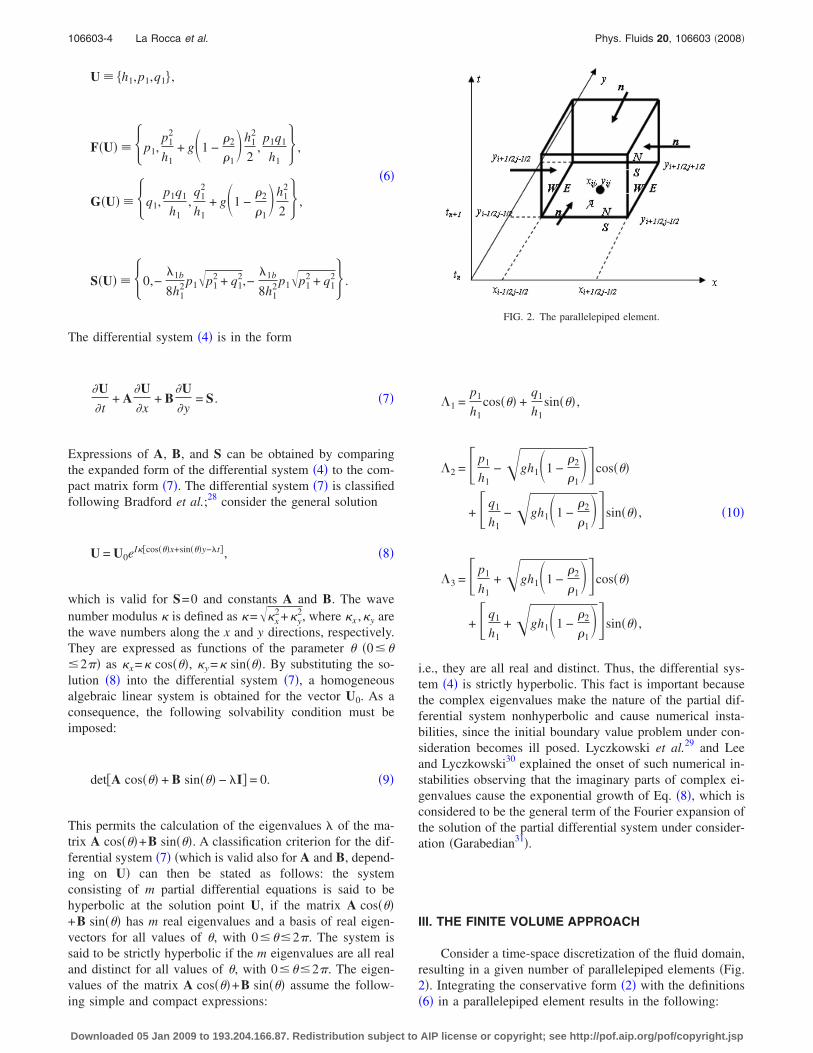
III. THE FINITE VOLUME APPROACH

Consider a time-space discretization of the fluid domain,resulting in a given number of parallelepiped elements �Fig.2�. Integrating the conservative form �2� with the definitions�6� in a parallelepiped element results in the following:

FIG. 2. The parallelepiped element.

106603-4 La Rocca et al. Phys. Fluids 20, 106603 �2008�

Downloaded 05 Jan 2009 to 193.204.166.87. Redistribution subject to AIP license or copyright; see http://pof.aip.org/pof/copyright.jsp

�A

�Un+1 − Un�dA − �tn

tn+1 ��A

�F�U�nx + G�U�ny�dBdt

− �tn

tn+1 �A

SdAdt = 0. �11�

Defining a spatially averaged value of U on A �the spacecell� given by

Un+1 =1

A�AUn+1dA ,

�12�

Un =1

A�AUndA ,

the following scheme is obtained from Eq. �11�:

Un+1 = Un +1

A�tn

tn+1 ��A

�F�U�nx + G�U�ny�dBdt

+1

A�tn

tn+1 �A

SdAdt . �13�

Calculating the intercell fluxes on the right hand side of Eq.�13� presents a difficulty because knowledge of the solutionU is required on the lateral surfaces of the parallelepipedelement in Fig. 2. This problem is solved using an approxi-mate Riemann solver procedure; in this work Roe’s approxi-mate Riemann solver procedure is adopted �Toro18�.

The approximate procedure contains multiple steps.

First, the Jacobian matrices A=dF /dU �U=U , B=dG /dU �U=V are defined as functions of the average initial

values U= U�UW ,UE� , V= V�US ,UN� �see Fig. 2 for themeaning of the subscripts S, N, E, and W�. Second, the

eigenvalues of the Jacobian matrices i , i �i=1, . . . ,3��which are all real� and the corresponding right eigenvectors

Kxi , Kyi �which are complete and linearly independent� aredetermined. Third, the initial state is expanded with respectto the eigenvector as

� = Kx−1UW, � = Kx

−1UE,

�14�� = Ky

−1US, � = Ky−1UN,

where Kx ,Ky are the matrices whose columns are the eigen-

vectors Kxi , Kyi, respectively. Fourth, the Godunov approxi-mation of the explicit system �13� is adopted in order tocalculate explicitly the quantity Un+1,

Un+1 = Un +�t

�x�Fi−1/2 − Fi+1/2� +

�t

�y�G j−1/2 − G j+1/2�

+1

�x�y�

tn

tn+1 �A

SdAdt . �15�

In Eq. �15�, the intercell fluxes �Fig. 2� are calculated byRoe’s approximate Riemann solver �Toro18�, and are writtenas

Fi�1/2 =FW + FE

2− �

k=1,3

��k − �k�2

�k�Kxk,

FW = F�UW�, FE = F�UE� ,

�16�

G j�1/2 =GN + GS

2− �

k=1,3

��k − �k�2

� k�Kyk,

GS = G�US�, GN = G�UN� .

The approximate numerical method is completed using anaveraging procedure performed on the initial values. In veryrecent work �Flåtten and Munkejord22�, a new averaging pro-cedure was developed for Roe’s approximate Riemann solverapplied to a 1D, two-phase motion. However, the presentwork adopts the averaging procedure developed by Chippadaet al.19 and applied to the framework of 2D shallow-waterequations,

U =h1W

−1/2UW + h1E−1/2UE

h1W−1/2 + h1E

−1/2 , V =h1S

−1/2US + h1N−1/2UN

h1S−1/2 + h1N

−1/2 . �17�

For this approximate procedure to be valid, it is necessary toensure consistency with the exact Jacobian, and also to en-sure that the Jacobian matrices preserve flux conservationacross discontinuities �Toro18�. Moreover, the time interval�t must satisfy the condition

�t � min �x

max,

�y

max , �18�

where max, max are the eigenvalues having the maximum

modulus and belonging to the sets i , i, respectively.

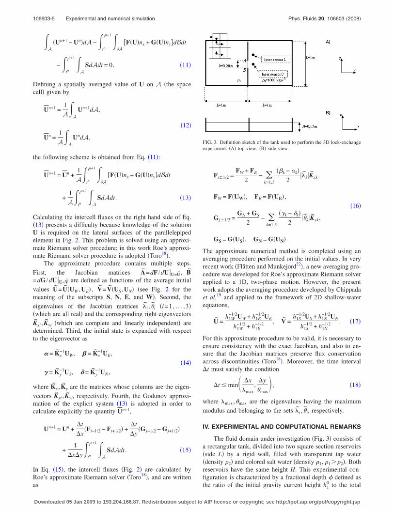
IV. EXPERIMENTAL AND COMPUTATIONAL REMARKS

The fluid domain under investigation �Fig. 3� consists ofa rectangular tank, divided into two square section reservoirs�side L� by a rigid wall, filled with transparent tap water�density �2� and colored salt water �density �1, �1��2�. Bothreservoirs have the same height H. This experimental con-figuration is characterized by a fractional depth � defined asthe ratio of the initial gravity current height h1

0 to the total

FIG. 3. Definition sketch of the tank used to perform the 3D lock-exchangeexperiment: �A� top view; �B� side view.

106603-5 Experimental and numerical simulation Phys. Fluids 20, 106603 �2008�

Downloaded 05 Jan 2009 to 193.204.166.87. Redistribution subject to AIP license or copyright; see http://pof.aip.org/pof/copyright.jsp

height H, such that �=1. At the center of the wall there is asliding gate AB with width b; after the gate is removed, thefluid bodies become in contact under nonequilibrium condi-tions, thereby originating the gravity current.

A charge coupled device video camera with an acquisi-tion frequency of 25 Hz records the evolution of the gravitycurrent, with time sampling occurring every 0.04 s; this issatisfactory for the present case. The images obtained by thefilm are recorded as rectangular matrices �576�768� of in-tegers, whose values lg, ranging from 0 to 255, represent thegray level of the corresponding pixel. The instantaneous stateof the gravity current is determined from changes of the graylevel value, caused by the chromatic contrast between thetwo density fluids. A suitable illumination system is used tostress this contrast; moreover, two laser sensors are used tomeasure the gravity current’s height at two fixed locations�Fig. 3�. The bottom surface of the tank is made rough bygluing onto it uniform sediment material, with a diameter �.The runs performed are listed in Table I. Runs 1 and 6 aremade with a smooth bottom surface. Each run is performedat least twice and the ensuing results are averaged.

Computationally, the fluid domain is divided into N ele-ments, and at the center of each the field variables h1 , p1 ,q1

are defined. This representation allows for a very easy impo-sition of boundary conditions. By introducing symmetricalvirtual elements outside the tank �Fig. 3�, no normal flowboundary conditions are imposed simply by setting the vir-tual values of the normal flux to the opposite values from thecorresponding real element.

The implementation of the numerical approach describedin Sec. III is straightforward. The CFL stability condition isset following Chippada et al.19 and assumes the expression

�t � inf d

max , �19�

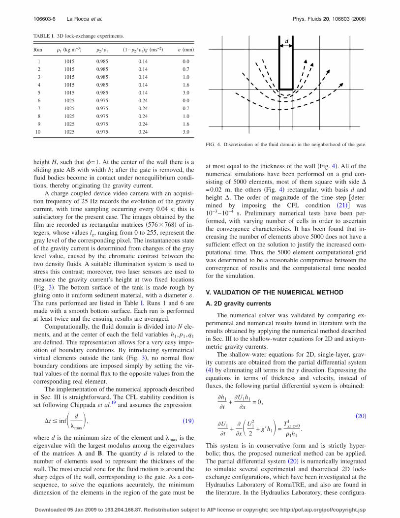
where d is the minimum size of the element and max is theeigenvalue with the largest modulus among the eigenvaluesof the matrices A and B. The quantity d is related to thenumber of elements used to represent the thickness of thewall. The most crucial zone for the fluid motion is around thesharp edges of the wall, corresponding to the gate. As a con-sequence, to solve the equations accurately, the minimumdimension of the elements in the region of the gate must be

at most equal to the thickness of the wall �Fig. 4�. All of thenumerical simulations have been performed on a grid con-sisting of 5000 elements, most of them square with side �=0.02 m, the others �Fig. 4� rectangular, with basis d andheight �. The order of magnitude of the time step �deter-mined by imposing the CFL condition �21�� was10−3–10−4 s. Preliminary numerical tests have been per-formed, with varying number of cells in order to ascertainthe convergence characteristics. It has been found that in-creasing the number of elements above 5000 does not have asufficient effect on the solution to justify the increased com-putational time. Thus, the 5000 element computational gridwas determined to be a reasonable compromise between theconvergence of results and the computational time neededfor the simulation.

V. VALIDATION OF THE NUMERICAL METHOD

A. 2D gravity currents

The numerical solver was validated by comparing ex-perimental and numerical results found in literature with theresults obtained by applying the numerical method describedin Sec. III to the shallow-water equations for 2D and axisym-metric gravity currents.

The shallow-water equations for 2D, single-layer, grav-ity currents are obtained from the partial differential system�4� by eliminating all terms in the y direction. Expressing theequations in terms of thickness and velocity, instead offluxes, the following partial differential system is obtained:

�h1

�t+

�U1h1

�x= 0,

�20��U1

�t+

�

�xU1

2

2+ g�h1 =

Txz1 �z=0

�1h1.

This system is in conservative form and is strictly hyper-bolic; thus, the proposed numerical method can be applied.The partial differential system �20� is numerically integratedto simulate several experimental and theoretical 2D lock-exchange configurations, which have been investigated at theHydraulics Laboratory of RomaTRE, and also are found inthe literature. In the Hydraulics Laboratory, these configura-

TABLE I. 3D lock-exchange experiments.

Run �1 �kg m−3� �2 /�1 �1−�2 /�1�g �ms−2� � �mm�

1 1015 0.985 0.14 0.0

2 1015 0.985 0.14 0.7

3 1015 0.985 0.14 1.0

4 1015 0.985 0.14 1.6

5 1015 0.985 0.14 3.0

6 1025 0.975 0.24 0.0

7 1025 0.975 0.24 0.7

8 1025 0.975 0.24 1.0

9 1025 0.975 0.24 1.6

10 1025 0.975 0.24 3.0

FIG. 4. Discretization of the fluid domain in the neighborhood of the gate.

106603-6 La Rocca et al. Phys. Fluids 20, 106603 �2008�

Downloaded 05 Jan 2009 to 193.204.166.87. Redistribution subject to AIP license or copyright; see http://pof.aip.org/pof/copyright.jsp

tions use a tank with length LT=3 m, width bT=0.2 m, andheight HT=0.4 m, containing a volume Vs=bTHx0 of saltwater ��1� and a volume Vw=bTH�LT−x0� of fresh water��2�. The initial length of the salt water reservoir is x0, set to0.2 m. Nine runs �VT1–VT9� were performed, using threedifferent values each for the density �1 and height H �TableII�. The system �20� has been integrated in the domain 0�x�xF�t�, where xF�t� is the instantaneous position of thefront. The following boundary and initial conditions wereapplied:

h1�x,0� = H, 0 � x � xF�0� ,

U1�x,0� = 0, 0 � x � xF�0� , �21�

U1�0,t� = 0, U1�xF�t�,t� = xF�t� ,

where H is the initial height of the heavier fluid and xF�t� isthe front velocity. To account for the time dependency of theintegration domain, a coordinate transformation is introduced�Bonnecaze et al.32�, which preserves the hyperbolic natureof the system and its conservative form. A proper physicaldefinition of the front velocity xF�t� must be adopted. Fol-lowing Ungarish,4 we adopt the Benjamin front velocity for-mula �Benjamin33�,

xF�t� = g�

rhF�t� �2 − �hF�t�/H���1 − �hF�t�/H��

1 + �hF�t�/H�,

�22�

where hF�t� is the instantaneous height of the front, i.e.,hF�t�=h1�xF�t� , t�, and r is the density ratio r=�2 /�1, where�2��1.

The numerical and experimental results from runs VT1–VT9 are compared in Fig. 5. These results are scaled using

T� =t

x0/ g�H, xf

� =xf

H. �23�

The experimental and numerical results corresponding to ex-periments with the same initial height collapse onto a singlecurve, but for the sake of clarity, each plot clusters the testswith the same density. The agreement is good for all consid-ered cases. Any differences between the numerical and ex-perimental results are likely due to the limitation of thesingle-layer approximation for gravity currents. Moreover,

these cases �Fig. 5� are with a smooth bottom surface, so thenumerical results have been obtained by setting the bottomstress term to zero.

Typical single-layer slumping results are shown in Fig.6. The triangles and diamonds show the results from Ungar-ish and Zemach,3 which were obtained by means of thesingle-layer approximation using the Benjamin formula �24�.The circles and squares show the numerical results from thepresent investigation, obtained using corresponding condi-tions. The represented quantities are scaled using hf

�=hf /h10,

uf�= xf / g�h1

0, �=h10 /H, and the height h1

0 is the initial height

TABLE II. 2D lock-exchange experiments.

Test �1 �kg /m3� H1 �m� �=H1 /H g� �m /s2�

VT1 1035 0.3 1 0.34

VT2 1035 0.2 1 0.34

VT3 1035 0.1 1 0.34

VT4 1065 0.3 1 0.61

VT5 1065 0.2 1 0.61

VT6 1065 0.1 1 0.61

VT7 1095 0.3 1 0.87

VT8 1095 0.2 1 0.87

VT9 1095 0.1 1 0.87

FIG. 5. Validation of the numerical method. Comparison between numericaland experimental time histories of the 2D gravity current’s front position.

FIG. 6. Validation of the numerical method. 2D single-layer model slump-ing results.

106603-7 Experimental and numerical simulation Phys. Fluids 20, 106603 �2008�

Downloaded 05 Jan 2009 to 193.204.166.87. Redistribution subject to AIP license or copyright; see http://pof.aip.org/pof/copyright.jsp

of the gravity current, generally different from H. The ratioof h1

0 to H is the fractional depth �. Good agreement isshown in Fig. 6.

B. Axisymmetric gravity currents

The axisymmetric single-layer shallow-water gravitycurrent equations are obtained formally from the partial dif-ferential system �20�, with a source term −U1h1 /x added tothe right hand side of the first equation,

�h1

�t+

�U1h1

�x= −

U1h1

x,

�24��U1

�t+

�

�xU1

2

2+ g�h1 =

Txz1 �z=0

�1h1,

where x is the radial coordinate. The system �24� has beenintegrated in the domain 0�x�xF�t�, using the same bound-ary and initial conditions �21�, where xF�t� is the instanta-neous radial position of the front. Following Ungarish,4 theempirical relation of Huppert and Simpson34 is adopted forthe front velocity definition,

xF�t� =1

2�hF�t�

H�−1/3 g�

rhF�t�, 0.075 �

hF�t�H

� 1,

�25�

xF�t� = 1.19 g�

rhF�t�, 0 �

hF�t�H

� 0.075.

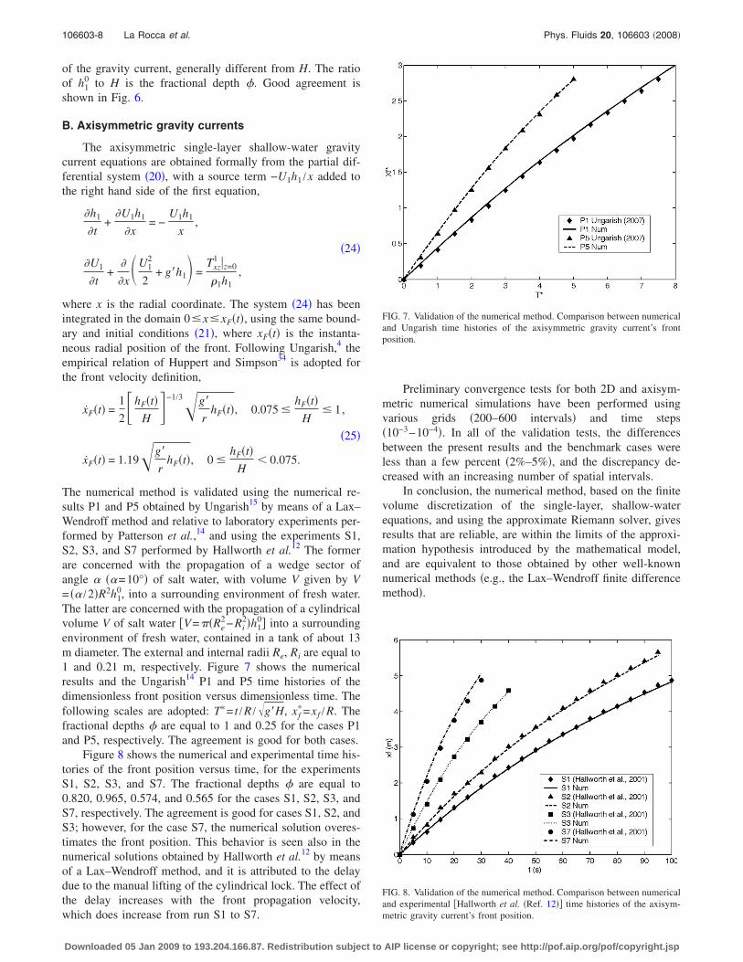
The numerical method is validated using the numerical re-sults P1 and P5 obtained by Ungarish15 by means of a Lax–Wendroff method and relative to laboratory experiments per-formed by Patterson et al.,14 and using the experiments S1,S2, S3, and S7 performed by Hallworth et al.12 The formerare concerned with the propagation of a wedge sector ofangle � ��=10°� of salt water, with volume V given by V= �� /2�R2h1

0, into a surrounding environment of fresh water.The latter are concerned with the propagation of a cylindricalvolume V of salt water �V=��Re

2−Ri2�h1

0� into a surroundingenvironment of fresh water, contained in a tank of about 13m diameter. The external and internal radii Re, Ri are equal to1 and 0.21 m, respectively. Figure 7 shows the numericalresults and the Ungarish14 P1 and P5 time histories of thedimensionless front position versus dimensionless time. Thefollowing scales are adopted: T�= t /R / g�H, xf

�=xf /R. Thefractional depths � are equal to 1 and 0.25 for the cases P1and P5, respectively. The agreement is good for both cases.

Figure 8 shows the numerical and experimental time his-tories of the front position versus time, for the experimentsS1, S2, S3, and S7. The fractional depths � are equal to0.820, 0.965, 0.574, and 0.565 for the cases S1, S2, S3, andS7, respectively. The agreement is good for cases S1, S2, andS3; however, for the case S7, the numerical solution overes-timates the front position. This behavior is seen also in thenumerical solutions obtained by Hallworth et al.12 by meansof a Lax–Wendroff method, and it is attributed to the delaydue to the manual lifting of the cylindrical lock. The effect ofthe delay increases with the front propagation velocity,which does increase from run S1 to S7.

Preliminary convergence tests for both 2D and axisym-metric numerical simulations have been performed usingvarious grids �200–600 intervals� and time steps�10−3–10−4�. In all of the validation tests, the differencesbetween the present results and the benchmark cases wereless than a few percent �2%–5%�, and the discrepancy de-creased with an increasing number of spatial intervals.

In conclusion, the numerical method, based on the finitevolume discretization of the single-layer, shallow-waterequations, and using the approximate Riemann solver, givesresults that are reliable, are within the limits of the approxi-mation hypothesis introduced by the mathematical model,and are equivalent to those obtained by other well-knownnumerical methods �e.g., the Lax–Wendroff finite differencemethod�.

FIG. 7. Validation of the numerical method. Comparison between numericaland Ungarish time histories of the axisymmetric gravity current’s frontposition.

FIG. 8. Validation of the numerical method. Comparison between numericaland experimental �Hallworth et al. �Ref. 12�� time histories of the axisym-metric gravity current’s front position.

106603-8 La Rocca et al. Phys. Fluids 20, 106603 �2008�

Downloaded 05 Jan 2009 to 193.204.166.87. Redistribution subject to AIP license or copyright; see http://pof.aip.org/pof/copyright.jsp

VI. ANALYSIS OF RESULTS

A. Advancing of the front: Numericaland experimental results

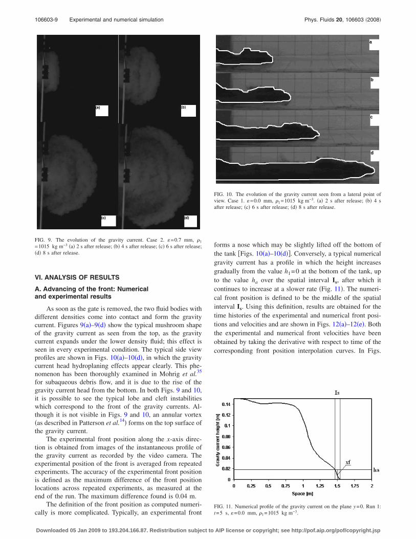
As soon as the gate is removed, the two fluid bodies withdifferent densities come into contact and form the gravitycurrent. Figures 9�a�–9�d� show the typical mushroom shapeof the gravity current as seen from the top, as the gravitycurrent expands under the lower density fluid; this effect isseen in every experimental condition. The typical side viewprofiles are shown in Figs. 10�a�–10�d�, in which the gravitycurrent head hydroplaning effects appear clearly. This phe-nomenon has been thoroughly examined in Mohrig et al.35

for subaqueous debris flow, and it is due to the rise of thegravity current head from the bottom. In both Figs. 9 and 10,it is possible to see the typical lobe and cleft instabilitieswhich correspond to the front of the gravity currents. Al-though it is not visible in Figs. 9 and 10, an annular vortex�as described in Patterson et al.14� forms on the top surface ofthe gravity current.

The experimental front position along the x-axis direc-tion is obtained from images of the instantaneous profile ofthe gravity current as recorded by the video camera. Theexperimental position of the front is averaged from repeatedexperiments. The accuracy of the experimental front positionis defined as the maximum difference of the front positionlocations across repeated experiments, as measured at theend of the run. The maximum difference found is 0.04 m.

The definition of the front position as computed numeri-cally is more complicated. Typically, an experimental front

forms a nose which may be slightly lifted off the bottom ofthe tank �Figs. 10�a�–10�d��. Conversely, a typical numericalgravity current has a profile in which the height increasesgradually from the value h1=0 at the bottom of the tank, upto the value ha over the spatial interval Is, after which itcontinues to increase at a slower rate �Fig. 11�. The numeri-cal front position is defined to be the middle of the spatialinterval Is. Using this definition, results are obtained for thetime histories of the experimental and numerical front posi-tions and velocities and are shown in Figs. 12�a�–12�e�. Boththe experimental and numerical front velocities have beenobtained by taking the derivative with respect to time of thecorresponding front position interpolation curves. In Figs.

FIG. 9. The evolution of the gravity current. Case 2. �=0.7 mm, �1

=1015 kg m−3 �a� 2 s after release; �b� 4 s after release; �c� 6 s after release;�d� 8 s after release.

FIG. 10. The evolution of the gravity current seen from a lateral point ofview. Case 1. �=0.0 mm, �1=1015 kg m−3. �a� 2 s after release; �b� 4 safter release; �c� 6 s after release; �d� 8 s after release.

FIG. 11. Numerical profile of the gravity current on the plane y=0. Run 1:t=5 s, �=0.0 mm, �1=1015 kg m−3.

106603-9 Experimental and numerical simulation Phys. Fluids 20, 106603 �2008�

Downloaded 05 Jan 2009 to 193.204.166.87. Redistribution subject to AIP license or copyright; see http://pof.aip.org/pof/copyright.jsp

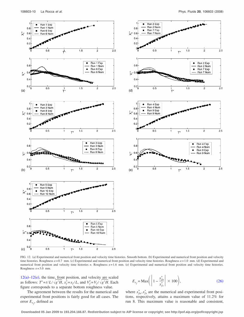
12�a�–12�e�, the time, front position, and velocity are scaledas follows: T�= t /L / g�H, xf

�=xf /L, and Vf�=Vf / g�H. Each

figure corresponds to a separate bottom roughness value.The agreement between the results for the numerical and

experimental front positions is fairly good for all cases. Theerror Exf

, defined as

Exf= Max�1 −

xfn�

xfs� � � 100 , �26�

where xfn� ,xfs

� are the numerical and experimental front posi-tions, respectively, attains a maximum value of 11.2% forrun 8. This maximum value is reasonable and consistent,

FIG. 12. �a� Experimental and numerical front position and velocity time histories. Smooth bottom. �b� Experimental and numerical front position and velocitytime histories. Roughness �=0.7 mm. �c� Experimental and numerical front position and velocity time histories. Roughness �=1.0 mm. �d� Experimental andnumerical front position and velocity time histories n. Roughness �=1.6 mm. �e� Experimental and numerical front position and velocity time histories.Roughness �=3.0 mm.

106603-10 La Rocca et al. Phys. Fluids 20, 106603 �2008�

Downloaded 05 Jan 2009 to 193.204.166.87. Redistribution subject to AIP license or copyright; see http://pof.aip.org/pof/copyright.jsp

with regard both to the limits of the mathematical model�single layer, immiscibility, etc.� and to the experimentaluncertainties.

The front position and the velocity time histories relativeto the different densities collapse onto a single curve for thesame surface roughness values. The main discrepancies be-tween the experimental and numerical results occur duringthe first instants of motion. These differences are probablydue to the numerical model being unable to account for themanual removal of the gate or for other physical features,such as the entrainment of the lower density fluid. The dif-ference in velocity between the numerical and experimentalresults is larger than the difference in front position; in par-ticular, the numerical front velocity is generally overesti-mated compared with the experimental one. The agreementin the velocity and front position improves as the flowevolves.

With the present experimental configuration, the analysisof the different motion phases is very difficult using the usualframework adopted for axisymmetric gravity currents�Ungarish15 and Patterson et al.14�. Qualitatively, the frontposition time histories for the 3D experiment are quite simi-lar to those for axisymmetric gravity currents �Pattersonet al.,14 Hallworth et al.,12 and Ungarish15�. By examiningthe front velocity plots it is possible to recognize two mainphases in the gravity current evolution: the first phase hasincreasing velocity, and the second phase has decreasing ve-locity. However, it is not possible to identify this first phaseas a “slumping” phase. This slumping phase, both in 2D andaxisymmetric gravity currents, is related �with reference to astandard lock-exchange experiment� to the propagation of adepression wave from the lock to the wall and from the wallto the gravity current front �Ungarish and Zemach3 andUngarish15�. As soon as the depression wave reaches thefront, the slumping phase is over and the velocity of the frontstarts to decrease; this is seen in both 2D and axisymmetricgravity currents.

In the present case, the backward-forward propagation ofthe depression wave is affected by the width of the gate andalso by the equal volumes of higher density fluid and lowerdensity fluid. Both the experimental and numerical observa-tions show that, as soon as the gate is removed, a fast back-ward depression wave propagates toward and reaches the leftwall �salt water reservoir side, see Fig. 3�. After that, thepresence of the gate, which chokes the flow, and the quantityof higher density fluid in the left reservoir cause the reser-voir’s level to decrease uniformly, maintaining a depthgreater than that of the gravity current expanding in the rightreservoir. Referring to the analysis performed by Ungarish,15

the forward propagation of the depression wave is hinderedby the choking effect of the gate, so that the depression wavenever reaches the gravity current front. After the aforemen-tioned first phase of gravity current evolution �approximatelyfor T��0.5�, when the velocity increases, the front velocitythen decreases �Figs. 12�a�–12�e��, as is seen during the “ter-tiary phase” of axisymmetric gravity currents. This behavior,which is separated from the backward-forward propagationof the depression wave and from the consequent evolution ofa slumping phase in the “classical” sense, can be explained

as follows. Neglecting the entrainment of lighter fluid, thefront velocity evolution is related to the front expansion,which occurs at a rate that balances the discharge of heavierfluid through the gate. This discharge of heavier fluidthrough the gate in turn depends on the geometry �ratio b /L�and the dynamics �gravity and friction forces�; it increaseswith the density difference ��1−�2� and decreases with theroughness �. The front velocity increases during the firstphase of the front evolution and decreases during the secondphase, so that the volume balance is preserved. Entrainmenteffects are important, and including these effects could resultin an improved agreement between the experimental and nu-merical results, mainly during the first phase of motion.However, the qualitative behavior described above would notbe altered by including entrainment.

Figures 13�a�–13�e� and 14�a�–14�e� compare the experi-mental and numerical gravity current fronts. The agreementis fairly good, in general. Along x=0, the experimental grav-ity current front differs from the numerical front. This dis-crepancy originates in the critical region immediately down-stream of the gate, where the curvature of the streamlines isvery large �Fig. 4�. However, such a discrepancy along x=0 decreases with time due to the declining influence of thegate region on the shape of the gravity current front withtime.

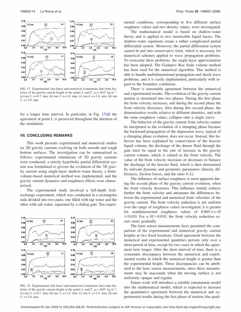
The effects of surface roughness on the gravity currentevolution are most apparent during the second phase of mo-tion. Such a result is in qualitative agreement with that ofHogg and Woods10 concerned with the influence of bottomfriction on 2D gravity currents: indeed they found that afteran initial phase of motion, governed by an inertial-buoyancybalance, a buoyancy-bottom friction phase starts. In thepresent case, during the second phase of motion the rough-ness causes a reduction in the front velocity which results inless distance traveled for any given time. Figure 15 shows aplot of the numerical and experimental nondimensional frontpositions xf

�, attained at t=10 s, versus the nondimensionalroughness � /H. Increasing the nondimensional roughness re-sults in a clear decrease in the achieved experimental andnumerical front positions at t=10 s. This decrease in dis-tance is not uniformly distributed, it occurs mainly within therange of 0.005�� /H�0.010. For a nondimensional rough-ness value � /H�0.010, the decrease in front position occursat a slower rate. The roughness effect also attenuates thedifference between the experimental and numerical front ve-locities �Figs. 12�a�–12�e�� and accelerates the beginning ofthe second phase in which the velocity decreases. In fact, theroughness increases the friction stress on the bottom surface;consequently, the discharge through the gate decreases sothat the beginning of the second phase occurs slightly earlier.

There are some systematic discrepancies between the ex-perimental and numerical results during the first phase �Figs.12�a�–12�e��. These discrepancies can be explained based onthe limits of the present formulation, for example, the ab-sence of entrainment in the model �Klemp et al.16�. In fact,the effect of entrainment could be significant due to both thegravity current increasing top surface and to the hydroplan-ing phenomenon, clearly visible in Figs. 10�a�–10�d�. Theonset of hydroplaning occurs when the stagnation pressure at

106603-11 Experimental and numerical simulation Phys. Fluids 20, 106603 �2008�

Downloaded 05 Jan 2009 to 193.204.166.87. Redistribution subject to AIP license or copyright; see http://pof.aip.org/pof/copyright.jsp

the gravity current front attains the same order of magnitudeas the hydrostatic pressure within the less dense fluid layerunder the gravity current. These conditions occur when Fr�0.35 �Mohrig et al.35�, corresponding to a Richardsonnumber �Ri=1 /Fr2� Ri�8.2. It is reasonable to relate thehydroplaning to the entrainment, since the lighter fluid layerunder the gravity current head is forced to enter the gravitycurrent from below as the front advances. Consequently, thedensity difference within the gravity current head decreases,resulting in an advancing velocity that is smaller than thatobtained from two perfectly immiscible layers. Entrainmenteffects on the gravity current top surface are negligible whenRi�0.8–1 �Fischer et al.23� because then stratification ef-fects dominate the flow relative to inertial effects, which areresponsible for entrainment. By estimating the Richardsonnumber using numerical results,

Ric =�1 − �2

�2

gh13

p12 + q1

2 , �27�

it can be seen that there is an area with Ric�0.8, so the twoentrainment effects described above could become relevantin the gravity current dynamics. This is illustrated in Figs.16�a� and 16�b� for runs 2 and 7 ��1=1015 kg m−3, �=0.7 mm; �1=1025 kg m−3, �=0.7 mm� at t=6 s. The

area where Ric�0.8 is located in the proximity of the front.This area is larger for run 2 �Fig. 16�a��, since the ratio ��1

−�2� /�2 is smaller for run 2 than for run 7. Including entrain-ment effects could enhance the quantitative agreement be-tween numerical and experimental results during the firstphase of the gravity current evolution, but it would notchange the qualitative agreement.

B. Experimental and numerical heightsof the gravity current

The height of the gravity current is measured using twolaser sensors �Fig. 3� at the points L and C. Each sensorgenerates a laser beam, which illuminates a spot on theopaque surface of the gravity current. The sensor “sees” thelight spot and computes the distance of the light spot fromthe sensor using triangulation. The laser beam has to passthrough the transparent lighter layer of water, and so it isrefracted. This could affect the reliability of the measure-ments; thus, a suitable preliminary sensor calibration wasperformed to account for the presence of transparent waterlayers of increasing height. The laser sensors perform bestwith a smooth, uniformly opaque surface. Unfortunately, thegravity current surface is neither smooth, because of insta-

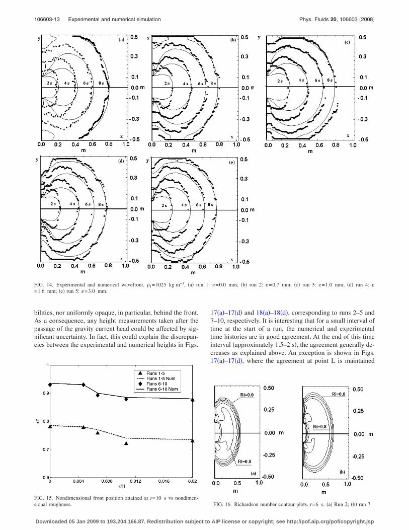
FIG. 13. Experimental and numerical wavefront. �1=1015 kg m−3, �a� run 1: �=0.0 mm; �b� run 2: �=0.7 mm; �c� run 3: �=1.0 mm; �d� run 4: �=1.6 mm; �e� run 5: �=3.0 mm.

106603-12 La Rocca et al. Phys. Fluids 20, 106603 �2008�

Downloaded 05 Jan 2009 to 193.204.166.87. Redistribution subject to AIP license or copyright; see http://pof.aip.org/pof/copyright.jsp

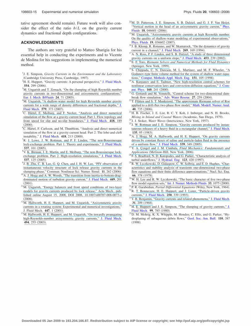
bilities, nor uniformly opaque, in particular, behind the front.As a consequence, any height measurements taken after thepassage of the gravity current head could be affected by sig-nificant uncertainty. In fact, this could explain the discrepan-cies between the experimental and numerical heights in Figs.

17�a�–17�d� and 18�a�–18�d�, corresponding to runs 2–5 and7–10, respectively. It is interesting that for a small interval oftime at the start of a run, the numerical and experimentaltime histories are in good agreement. At the end of this timeinterval �approximately 1.5–2 s�, the agreement generally de-creases as explained above. An exception is shown in Figs.17�a�–17�d�, where the agreement at point L is maintained

FIG. 14. Experimental and numerical wavefront. �1=1025 kg m−3, �a� run 1: �=0.0 mm; �b� run 2: �=0.7 mm; �c� run 3: �=1.0 mm; �d� run 4: �=1.6 mm; �e� run 5: �=3.0 mm.

FIG. 15. Nondimensional front position attained at t=10 s vs nondimen-sional roughness. FIG. 16. Richardson number contour plots. t=6 s. �a� Run 2; �b� run 7.

106603-13 Experimental and numerical simulation Phys. Fluids 20, 106603 �2008�

Downloaded 05 Jan 2009 to 193.204.166.87. Redistribution subject to AIP license or copyright; see http://pof.aip.org/pof/copyright.jsp

for a longer time interval. In particular, in Fig. 17�d� theagreement at point L is preserved throughout the duration ofthe simulation.

VII. CONCLUDING REMARKS

This work presents experimental and numerical studieson 3D gravity currents evolving on both smooth and roughbottom surfaces. The investigation can be summarized asfollows: experimental simulations of 3D gravity currentswere conducted, a strictly hyperbolic partial differential sys-tem was formulated to govern the evolution of the 3D grav-ity current using single-layer shallow-water theory, a finite-volume-based numerical method was implemented, and thegravity current dynamics and roughness effects were charac-terized.

The experimental study involved a full-depth lock-exchange experiment, which was conducted in a rectangulartank divided into two parts, one filled with tap water and theother with salt water, separated by a sliding gate. Ten experi-

mental conditions, corresponding to five different surfaceroughness values and two density values, were investigated.

The mathematical model is based on shallow-watertheory and is applied to two immiscible liquid layers. Theshallow-water equations create a rather complicated partialdifferential system. Moreover, the partial differential systemcannot be put into conservative form, which is necessary fornumerical schemes applied to wave propagation problems.To overcome these problems, the single-layer approximationhas been adopted. The Godunov–Roe finite volume methodhas been used for the numerical algorithm. This method isable to handle multidimensional propagation and shock waveproblems, and it is easily implemented, particularly with re-gard to the boundary conditions.

There is reasonable agreement between the numericaland experimental results. The evolution of the gravity currentmotion is structured into two phases. During the first phasethe front velocity increases, and during the second phase thefront velocity decreases. Also during this second phase, thedimensionless results relative to different densities, and withthe same roughness values, collapse onto a single curve.

The behavior of the gravity current front velocity cannotbe interpreted as the evolution of a slumping phase becausethe backward propagation of the depression wave, typical ofa slumping phase evolution, does not occur. Instead, this be-havior has been explained by conservation of the heavierliquid volume; the discharge of the denser fluid through thegate must be equal to the rate of increase in the gravitycurrent volume, which is related to the front velocity. Thevalue of the front velocity increases or decreases to balancethe discharge of the heavier fluid, which is then determinedby relevant dynamic and geometric parameters �density dif-ferences, friction forces, and the ratio b /L�.

The influence of surface roughness is most apparent dur-ing the second phase of the gravity current evolution, whenthe front velocity decreases. This influence mainly reducesfurther the front velocity and attenuates the differences be-tween the experimental and numerical front velocities of thegravity current. The front velocity reduction is not uniformover the range of roughness values investigated; it is greaterfor nondimensional roughness values of 0.005�� /H�0.010. For � /H�0.010, the front velocity reduction oc-curs more gradually.

The laser sensor measurements have permitted the com-parison of the experimental and numerical gravity currentheights at two fixed locations. Good agreement between thenumerical and experimental quantities persists only over ashort period of time, except for two cases in which the agree-ment lasts longer. After the short interval of time, there is asystematic discrepancy between the numerical and experi-mental results in which the numerical height is greater thanthe experimental height. These discrepancies can be attrib-uted to the laser sensor measurements, since these measure-ments may be inaccurate when the moving surface is notuniformly opaque and regular.

Future work will introduce a suitable entrainment modelinto the mathematical model, which is expected to increasethe quantitative agreement between the numerical and ex-perimental results during the first phase of motion �the quali-

FIG. 17. Experimental �dot lines� and numerical �continuous line� time his-tories of the gravity current height at the points L and C. �1=1015 kg m−3,�a� run 2: �=0.7 mm; �b� run 3: �=1.0 mm; �c� run 4: �=1.6 mm; �d� run5: �=3.0 mm.

FIG. 18. Experimental �dot lines� and numerical �continuous line� time his-tories of the gravity current height at the points L and C. �1=1025 kg m−3,�a� run 2: �=0.7 mm; �b� run 3: �=1.0 mm; �c� run 4: �=1.6 mm; �d� run5: �=3.0 mm.

106603-14 La Rocca et al. Phys. Fluids 20, 106603 �2008�

Downloaded 05 Jan 2009 to 193.204.166.87. Redistribution subject to AIP license or copyright; see http://pof.aip.org/pof/copyright.jsp

tative agreement should remain�. Future work will also con-sider the effect of the ratio b /L on the gravity currentdynamics and fractional depth configurations.

ACKNOWLEDGMENTS

The authors are very grateful to Matteo Sbarigia for hisessential help in conducting the experiments and to Vicentede Medina for his suggestions in implementing the numericalmethod.

1J. E. Simpson, Gravity Currents in the Environment and the Laboratory�Cambridge University Press, Cambridge, 1997�.

2H. E. Huppert, “Gravity currents: A personal perspective,” J. Fluid Mech.554, 299 �2006�.

3M. Ungarish and T. Zemach, “On the slumping of high Reynolds numbergravity currents in two-dimensional and axisymmetric configurations,”Eur. J. Mech. B/Fluids 24, 71 �2005�.

4M. Ungarish, “A shallow-water model for high Reynolds number gravitycurrents for a wide range of density differences and fractional depths,” J.Fluid Mech. 579, 373 �2007�.

5C. Härtel, E. Meiburg, and F. Necker, “Analysis and direct numericalsimulation of the flow at a gravity-current head. Part 1. Flow topology andfront speed for slip and no-slip boundaries,” J. Fluid Mech. 418, 189�2000�.

6C. Härtel, F. Carlsson, and M. Thunblom, “Analysis and direct numericalsimulation of the flow at a gravity-current head. Part 2. The lobe-and-cleftinstability,” J. Fluid Mech. 418, 213 �2000�.

7R. J. Lowe, J. W. Rottman, and P. F. Linden, “The non-Boussinesquelock-exchange problem. Part 1. Theory and experiments,” J. Fluid Mech.537, 101 �2005�.

8V. K. Birman, J. E. Martin, and E. Meiburg, “The non-Boussinesque lock-exchange problem. Part 2. High-resolution simulations,” J. Fluid Mech.537, 125 �2005�.

9J. B. Zhu, C. B. Lee, G. Q. Chen, and J. H. W. Lee, “PIV observation ofinstantaneous velocity structure of lock release gravity currents in theslumping phase,” Commun. Nonlinear Sci. Numer. Simul. 11, 262 �2006�.

10A. J. Hogg and A. W. Woods, “The transition from inertia-to-bottom-drag-dominated motion of turbulent gravity current,” J. Fluid Mech. 449, 201�2001�.

11M. Ungarish, “Energy balances and front speed conditions of two-layermodels for gravity currents produced by lock release,” Acta Mech., pub-lished online August 15, 2008, DOI 2008, 10.1007/s00707-008-0073-z�2008�.

12M. Hallworth, H. E. Huppert, and M. Ungarish, “Axisymmetric gravitycurrents in a rotating system: Experimental and numerical investigations,”J. Fluid Mech. 447, 1 �2001�.

13M. Hallworth, H. E. Huppert, and M. Ungarish, “On inwardly propagatinghigh-Reynolds-number axisymmetric gravity currents,” J. Fluid Mech.494, 255 �2003�.

14M. D. Patterson, J. E. Simpson, S. B. Dalziel, and G. J. F. Van Heijst,“Vortical motion in the head of an axisymmetric gravity current,” Phys.Fluids 18, 046601 �2006�.

15M. Ungarish, “Axisymmetric gravity currents at high Reynolds number:On the quality of shallow-water modeling of experimental observations,”Phys. Fluids 19, 036602 �2007�.

16J. B. Klemp, R. Rotunno, and W. Skamarock, “On the dynamics of gravitycurrent in a channel,” J. Fluid Mech. 269, 169 �1994�.

17A. N. Ross, P. F. Linden, and S. B. Dalziel, “A study of three dimensionalgravity currents on a uniform slope,” J. Fluid Mech. 453, 239 �2002�.

18E. F. Toro, Riemann Solvers and Numerical Methods for Fluid Dynamics�Springer, New York, 1999�.

19S. Chippada, C. N. Dawson, M. L. Martinez, and M. F. Wheeler, “AGodunov-type finite volume method for the system of shallow water equa-tions,” Comput. Methods Appl. Mech. Eng. 151, 105 �1998�.

20A. Kurganov and E. Tadmor, “New high-resolution central schemes fornonlinear conservation laws and convection-diffusion equations,” J. Com-put. Phys. 160, 241 �2000�.

21G. Gottardi and M. Venutelli, “Central scheme for two-dimensional dam-break flow simulation,” Adv. Water Resour. 27, 259 �2004�.

22T. Flåtten and S. T. Munkejord, “The approximate Riemann solver of Roeapplied to a drift-flux two-phase flow model,” Math. Modell. Numer. Anal.40, 735 �2006�.

23H. B. Fischer, J. E. List, R. C. Y. Koh, J. Imberger, and N. H. Brooks,Mixing in Inland and Coastal Waters �Academic, San Diego, 1979�.

24J. J. Stoker, Water Waves �Interscience, New York, 1957�.25J. W. Rottman and J. E. Simpson, “Gravity currents produced by instan-

taneous releases of a heavy fluid in a rectangular channel,” J. Fluid Mech.135, 95 �1983�.

26A. J. Hogg, M. A. Hallworth, and H. E. Huppert, “On gravity currentsdriven by constant fluxes of saline and particle-laden fluid in the presenceof a uniform flow,” J. Fluid Mech. 539, 349 �2005�.

27Y. A. Çengel and J. M. Cimbala, Fluid Mechanics: Fundamentals andApplications �McGraw-Hill, New York, 2006�.

28F. S. Bradford, N. D. Katopodes, and G. Parker, “Characteristic analysis ofturbid underflows,” J. Hydraul. Eng. 123, 420 �1997�.

29R. W. Lyczkowski, D. Gidaspow, C. W. Solbrig, and E. D. Hughes, “Char-acteristics and stability analysis of transients one-dimensional two-phaseflow equations and their finite difference approximations,” Nucl. Sci. Eng.66, 378 �1978�.

30W. H. Lee and R. W. Lyczkowski, “The basic character of five two-phaseflow model equation sets,” Int. J. Numer. Methods Fluids 33, 1075 �2000�.

31P. R. Garabedian, Partial Differential Equations �Wiley, New York, 1964�.32R. T. Bonnecaze, H. E. Huppert, and J. Lister, “Particle-driven gravity

currents,” J. Fluid Mech. 250, 339 �1993�.33T. B. Benjamin, “Gravity currents and related phenomena,” J. Fluid Mech.

31, 209 �1968�.34H. E. Huppert and J. E. Simpson, “The slumping of gravity currents,” J.

Fluid Mech. 99, 785 �1980�.35D. M. Mohrig, K. X. Whipple, M. Hondzo, C. Ellis, and G. Parker, “Hy-

droplaning of subaqueous debris flows,” Geol. Soc. Am. Bull. 110, 387�1998�.

106603-15 Experimental and numerical simulation Phys. Fluids 20, 106603 �2008�

Downloaded 05 Jan 2009 to 193.204.166.87. Redistribution subject to AIP license or copyright; see http://pof.aip.org/pof/copyright.jsp