Experimental and Numerical Investigation of Tire Tread Wear ...

lubricants

Article

Experimental and Numerical Investigation of Tire Tread Wearon Block Level

Felix Hartung 1, Mario Alejandro Garcia 1, Thomas Berger 1, Michael Hindemith 2, Matthias Wangenheim 2

and Michael Kaliske 1,*

�����������������

Citation: Hartung, F.; Garcia, M.A.;

Berger, T.; Hindemith, M.;

Wangenheim, M.; Kaliske, M.

Experimental and Numerical

Investigation of Tire Tread Wear on

Block Level. Lubricants 2021, 9, 113.

https://doi.org/10.3390/

lubricants9120113

Academic Editor: Maria Dolores

Bermudez

Received: 6 October 2021

Accepted: 16 November 2021

Published: 23 November 2021

Publisher’s Note: MDPI stays neutral

with regard to jurisdictional claims in

published maps and institutional affil-

iations.

Copyright: © 2021 by the authors.

Licensee MDPI, Basel, Switzerland.

This article is an open access article

distributed under the terms and

conditions of the Creative Commons

Attribution (CC BY) license (https://

creativecommons.org/licenses/by/

4.0/).

1 Institute for Structural Analysis, Technische Universität Dresden, 01062 Dresden, Germany;[email protected] (F.H.); [email protected] (M.A.G.);[email protected] (T.B.)

2 Institute of Dynamics and Vibration Research, Leibniz Universität Hannover, 30167 Hannover, Germany;[email protected] (M.H.); [email protected] (M.W.)

* Correspondence: [email protected]

Abstract: Tread wear appears as a consequence of friction, which mainly depends on surface charac-teristics, contact pressure, slip velocity, temperature and dissipative material properties of the treadmaterial itself. The subsequent description introduces a wear model as a function of the frictionalenergy rate. A post-processing as well as an adaptive re-meshing algorithm are implemented into afinite element code in order to predict wear loss in terms of mass. The geometry of block models isgenerated by image processing tools using photographs of the rubber samples in the laboratory. Inaddition, the worn block shape after the wear test is compared to simulation results.

Keywords: wear; friction; finite element method; adaptive meshing; linear friction test; image processing

1. Introduction

The tire is the only contact between vehicles and road surfaces and, thus, it has animportant function: it must transmit all forces and moments in all spatial directions asreliably as possible. It is known that in tire design, compromises must be found betweenfunctional goals, in particular (wet) braking, mileage, rolling resistance, and noise emis-sion [1]. In addition, wear particle emission comes more and more into focus of legislativeinstitutions [2]. Looking closer into the construction of tires with its many rubber layers,textile plies, and steel belts, the one that is in contact with the road is the tire tread, which isusually geometrically subdivided into blocks of different size or circumferential ribs. Hence,all contact forces and moments are transmitted via the tire tread and it is the tread sufferingwear and emitting wear particles. In literature, the wear rate of rubber compounds is oftendescribed by a function proportional to the frictional power dissipated during contact,while the frictional power is directly dependent on the local sliding speed, the local contactpressure, and the coefficient of dynamic friction (compare e.g., [3–5]). The force that canbe transmitted between tire and road is determined by the local friction characteristicswhich is composed of static friction in the sticking zone of the contact patch and dynamicfriction in the sliding zone [6]. Besides the road surface quality and the rubber materialformulation, it is known that the dynamic coefficient of friction between rubber and a roughsurface depends on a number of parameters, in particular local contact pressure, slidingvelocity, and the contact temperature are of great importance. These parameters are a directconsequence of the tire construction and the maneuvers in which the tire undergoes.

Linear friction testers (in this case HiLiTe [7] was used) are a common methodologyto assess friction between tire tread blocks and (road) surface sections [8]. These devicesare used to quasi-steadily investigate characteristics of the coefficient of sliding frictionin a wide parameter range, i.e., contact pressure, sliding speed, and in some cases alsoambient temperature are varied but held constant during a single test run. The range of

Lubricants 2021, 9, 113. https://doi.org/10.3390/lubricants9120113 https://www.mdpi.com/journal/lubricants

Lubricants 2021, 9, 113 2 of 29

parameters is defined to cover all relevant situations (e.g., ABS braking or cornering) thetest is intended to represent.

In this paper, it is described for the first time how a linear friction tester is used toquasi-steadily characterize not only tread block friction but also tire tread wear, feedingFinite Element (FE) based tread block friction, and wear simulations. The tread block modeldemands for a number of parameter sets that are direct outcomes of these experiments,in particular the friction characteristics in terms of local contact pressure and slidingspeed and the wear characteristics in terms of contact pressure, sliding speed, and localcoefficient of friction. Furthermore, the tread block model consists of a material descriptioncovering all important effects, in this case a viscoelastic rubber material model, whoseparameters are assessed by uni-, biaxial tension, and pure shear tests as well as the DynamicMechanical Analysis (DMA). A self-evident but important constraint is that friction andwear experiments are performed in a parameter range covering the full parameter space ofthe simulations. Experimentally, quasi-steadiness is achieved by conditioning of the block,i.e., the block slides a number of runs before measurement starts, to gain an initial wearshape as well as attaining a steady-state temperature [9]. In FE simulations, wear resultsin loss of material, even if parameters and simulations are performed quasi-steadily. Onemethod to take volume loss into account is recurring re-meshing of the block geometry (see,e.g., [3,4,10,11]). In this paper, a novel method is presented to perform mesh generation andre-meshing based on automatic image processing of the tread block shape during linearfriction tester experiments. Hence, a good agreement between simulations and friction andwear tests can be achieved.

2. Materials and Methods2.1. Experimental Setup

For the experiments we made use of the High-speed Linear Tester (HiLiTe, see Figure 1)at the Institute of Dynamics and Vibration Research (IDS) at Leibniz Universität Hannover.

concrete foundatation

measuring capsule

synchronous

servo motor

(a)

mount of test surface

force transducer

bellows cylinder

to apply normal force

rubber sample

(b)

Figure 1. High-Speed Linear Tester (HiLiTe) for friction and wear measurements. (a) Overall view, (b) Detail lateral view.

A tread block sample is pressed onto a test track with a defined normal force and slideswith a defined velocity profile relative to the track. With this type of motion, the slidingprocess between tire tread and road surface of a rolling tire under slip is replicated. Hence,HiLiTe’s sliding velocity corresponds to the velocity difference between tire circumferentialspeed and vehicle speed, e.g., during acceleration or braking. The sliding speed rangecovered by HiLiTe in the current configuration is up to 10 m/s. The normal force betweentire tread bock and counter surface can be selected up to 1000 N. This enables testingpassenger car tread blocks as well as truck or aircraft treads in dependence of the samplesize and, in particular, its contact area. The normal force during a test is set in relation tothe pneumatic tire pressure to be replicated multiplied with the nominal contact area of thetread block, which is typically at least 20× 20 mm2 at a maximum height of 10 mm to limitblock distortion. HiLiTe is located in a climate chamber, where temperature and humidity

Lubricants 2021, 9, 113 3 of 29

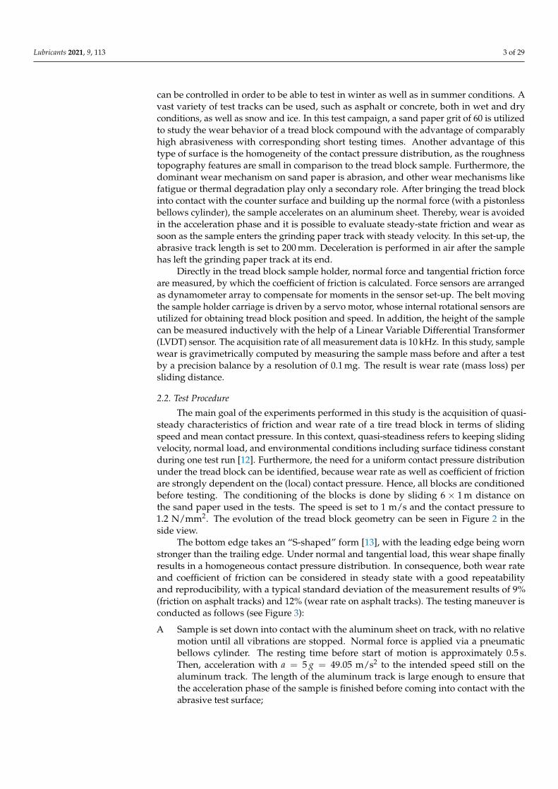
can be controlled in order to be able to test in winter as well as in summer conditions. Avast variety of test tracks can be used, such as asphalt or concrete, both in wet and dryconditions, as well as snow and ice. In this test campaign, a sand paper grit of 60 is utilizedto study the wear behavior of a tread block compound with the advantage of comparablyhigh abrasiveness with corresponding short testing times. Another advantage of thistype of surface is the homogeneity of the contact pressure distribution, as the roughnesstopography features are small in comparison to the tread block sample. Furthermore, thedominant wear mechanism on sand paper is abrasion, and other wear mechanisms likefatigue or thermal degradation play only a secondary role. After bringing the tread blockinto contact with the counter surface and building up the normal force (with a pistonlessbellows cylinder), the sample accelerates on an aluminum sheet. Thereby, wear is avoidedin the acceleration phase and it is possible to evaluate steady-state friction and wear assoon as the sample enters the grinding paper track with steady velocity. In this set-up, theabrasive track length is set to 200 mm. Deceleration is performed in air after the samplehas left the grinding paper track at its end.

Directly in the tread block sample holder, normal force and tangential friction forceare measured, by which the coefficient of friction is calculated. Force sensors are arrangedas dynamometer array to compensate for moments in the sensor set-up. The belt movingthe sample holder carriage is driven by a servo motor, whose internal rotational sensors areutilized for obtaining tread block position and speed. In addition, the height of the samplecan be measured inductively with the help of a Linear Variable Differential Transformer(LVDT) sensor. The acquisition rate of all measurement data is 10 kHz. In this study, samplewear is gravimetrically computed by measuring the sample mass before and after a testby a precision balance by a resolution of 0.1 mg. The result is wear rate (mass loss) persliding distance.

2.2. Test Procedure

The main goal of the experiments performed in this study is the acquisition of quasi-steady characteristics of friction and wear rate of a tire tread block in terms of slidingspeed and mean contact pressure. In this context, quasi-steadiness refers to keeping slidingvelocity, normal load, and environmental conditions including surface tidiness constantduring one test run [12]. Furthermore, the need for a uniform contact pressure distributionunder the tread block can be identified, because wear rate as well as coefficient of frictionare strongly dependent on the (local) contact pressure. Hence, all blocks are conditionedbefore testing. The conditioning of the blocks is done by sliding 6 × 1 m distance onthe sand paper used in the tests. The speed is set to 1 m/s and the contact pressure to1.2 N/mm2. The evolution of the tread block geometry can be seen in Figure 2 in theside view.

The bottom edge takes an “S-shaped” form [13], with the leading edge being wornstronger than the trailing edge. Under normal and tangential load, this wear shape finallyresults in a homogeneous contact pressure distribution. In consequence, both wear rateand coefficient of friction can be considered in steady state with a good repeatabilityand reproducibility, with a typical standard deviation of the measurement results of 9%(friction on asphalt tracks) and 12% (wear rate on asphalt tracks). The testing maneuver isconducted as follows (see Figure 3):

A Sample is set down into contact with the aluminum sheet on track, with no relativemotion until all vibrations are stopped. Normal force is applied via a pneumaticbellows cylinder. The resting time before start of motion is approximately 0.5 s.Then, acceleration with a = 5 g = 49.05 m/s2 to the intended speed still on thealuminum track. The length of the aluminum track is large enough to ensure thatthe acceleration phase of the sample is finished before coming into contact with theabrasive test surface;

Lubricants 2021, 9, 113 4 of 29

B Leaving the aluminum sheet and coming into contact with the abrasive surface. Shortphase of vertical dynamics because of the step down to the track with respectiveeffects in signal of coefficient of friction;

C Overcoming the static friction of the sample on the abrasive counter surface. Forthe transfer of results to rolling friction, assessment of the static friction coefficientis essential due to the large contribution of the sticking zone to the tangential forcesin the tire footprint. Transitioning from sticking to sliding requires some time, inparticular steady-state temperatures and block deflection have to be established. Inthis transition period, the coefficient of friction decreases slightly. The transitiontime lag constants are specific for the respective frictional contact and affected bymaterials, surface topographies, and potential third media in contact. Subsequently,a quasi-steady period of sliding friction occurs with a constant level of coefficient offriction, which is evaluated as the steady-state coefficient of friction;

D At the end of the test track, the sample is decelerated and leaves the contact.

sliding direction

1

2

3

4

5

6

Figure 2. Pre-conditioning.

This approach enables us to define the sliding distance as exact as possible and ensuresthat abrasion occurs under quasi-steady conditions without interferences by tread blocklongitudinal dynamics. The friction and wear tests are repeated with five conditionedsamples with very good repeatability as shown in Figure 3.

0 1 2 3 4 5 60

0.5

1

1.5A B C D

rang

efo

rca

lcul

atin

gm

ean

valu

e

time in s

coef

ficie

ntof

fric

tion

test run 1test run 2test run 3test run 4test run 5

Figure 3. Test repetitions at p = 0.4 N/mm2 and v = 50 mm/s.

Lubricants 2021, 9, 113 5 of 29

After each single test run, the track is cleaned from rubber debris with compressedair and a soft brush. In case of material transfer to the track, rubber layers can be cleanedby manual wiping with uncured natural rubber (NR). The samples are disassembledfrom the test rig and weighed every 1 to 20 cycles (depending on the abrasion rate) afterblowing loose particles from the sample surface by compressed air. Since the coefficient offriction on the aluminum sheet adjusts with a time delay during the acceleration phase, theacceleration time t = 50 mm/s

49.05 m/s2 ≈ 0.001 s does not coincide with the time until the frictioncoefficient is steady state between points A and B in Figure 3.

2.3. Material Model for Rubber

Rubber material is characterized by non-linear elasticity at large strains (hyperelas-ticity), time dependent effects due to viscoelasticity, and consists of an isochoric (volume-preserving) and a volume changing contribution. To capture a wide range of frequen-cies, the generalized MAXWELL model, which is shown in Figure 4, is chosen for theisochoric part.

E∞

E1 Ek En

τnτkτ1

σ

σ

σeq σneq,k σneq,nσneq,1

Figure 4. Material rheology for isochoric part (generalized MAXWELL model).

The first branch of the generalized MAXWELL model (equilibrium branch) consistsof a single spring with the so-called long-term stiffness E∞ = γ∞ E0 (stiffness at quasi-static loads), where E0 represents the instantaneous stiffness of the entire rheologicalmodel (stiffness at very high dynamic loads). The remaining branches are MAXWELL

elements (non-equilibrium branches) in parallel. Each MAXWELL element is composedof a spring with the spring stiffness Ek (k = 1, . . . , n) and a dashpot with the dynamicviscosity ηk = Ek τk, where τk is the relaxation time of dashpot k. In small strain theory, theone-dimensional strain of a MAXWELL element

ε = εe + εv (1)

is the sum of the elastic and the viscous strain, whereas the stress in both, spring anddashpot, are identical. By inserting εe = σneq,k/Ek and εv = σneq,k/Ek τk in the first timederivative of Equation (1), the differential equation

Ek ε = σneq,k +σneq,k

τk(2)

Lubricants 2021, 9, 113 6 of 29

of MAXWELL element k is derived. Equation (2) is a linear rate equation. By inserting theEULERian representation regarding stresses

σk = σk exp(iωt) (3)

and strainsε = ε exp[i(ωt− δ)] , (4)

with i :=√−1, stress amplitude σk, strain amplitude ε and δ as phase shift between stress

and strain response in Equation (2), the differential equation

iωτk Ek ε = σk exp(iδ) (1 + iωτk) (5)

is solved for an oscillation in the complex plane. This formulation defines the complex modulus

E∗k =σkε

exp(iδ) = Ekiωτk

1 + iωτk(6)

of MAXWELL element k within the generalized MAXWELL model. The complex modulusE∗k = E′k + iE′′k can be decomposed into a real contribution (storage modulus) and animaginary part (loss modulus). By use of the normalized stiffness factors γk = Ek/E0 with

γ∞ +n∑

k=1γk = 1, the storage modulus

E′ = γ∞E0 +n

∑k=1

(ω τk)2

1 + (ω τk)2 γk E0 (7)

and the loss modulus

E′′ =n

∑k=1

ω τk

1 + (ω τk)2 γk E0 (8)

of the entire generalized MAXWELL model are determined as function of frequencyf = 2 π/ω.

For the three-dimensional constitutive law, a continuum model based on large straintheory is applied. The small strain formulation is expanded by introducing the defor-mation gradient F = ∂x/∂X that maps point coordinates of the continuum from referenceX to current configuration x. The deformation gradient of one MAXWELL element at amaterial point

F = Fvol Fiso =(

J−1/3 1)(Fe Fv) (9)

can be split multiplicatively into a volumetric and an isochoric part, whereby the latter iscomposed of an elastic and a viscoelastic contribution. In the considered case, J = det F > 0stands for the ratio of volume change, which is nearly one for rubber-like materials. Theright CAUCHY-GREEN tensor C = FT F and left CAUCHY-GREEN tensor b = F FT describethe strain in the reference and the current configuration, respectively. In contrast to themultiplicative split of F, the stress state of the generalized MAXWELL model in the referenceconfiguration is described by the second PIOLA-KIRCHHOFF stress tensor

S = Svol + Siso = Svol + Seq +n

∑k=1

Sneq,k (10)

additively. In analogy to the stress tensor, the tangent modulus

C = Cvol +Ciso = Cvol +Ceq +n

∑k=1Cneq,k (11)

Lubricants 2021, 9, 113 7 of 29

in the reference configuration is obtained. Based on linear viscoelasticity, the differentialequation for MAXWELL element k

γk Seq = Sneq,k +1τk

Sneq,k (12)

is derived from Equation (2). Equation (12) is described in the reference configuration topreserve objectivity. The non-equilibrium stress of MAXWELL element k

Sneq,k(tj+1

)= γk

tj+1∫

t=0

exp(− tj+1 − t

τk

) dSeq(t)dt

dt

= exp(−∆t

τk

)Sneq,k

(tj)+ γk

1− exp(−∆t/τk)∆t/τk

[Seq(tj+1

)− Seq

(tj)]

,

(13)

with the time increment ∆t = tj+1 − tj, is computed by a recurrence relation solving theconvolution integral (see [14]). Note that the application of Equation (13) reduces thecomputational costs significantly, because the current stress state is computed from thestresses at the previous time step tj. The derivative of the isochoric part of the second PIOLA-KIRCHHOFF stress tensor with respect to the corresponding right CAUCHY-GREEN tensor

Ciso(tj+1

)= 2

∂Siso(tj+1

)

∂Ciso(tj+1

) =

[1 +

n

∑k=1

1− exp(−∆t/τk)∆t/τk

]Ceq

(tj+1

)(14)

yields the three-dimensional formulation of the tangent modulus of the rheology modelin Figure 4 for large strains in the reference configuration. Thus, the isochoric materialtangent results from the current isochoric material tangent of the equilibrium branch at tj+1due to the recursive formulation of Equation (13). In order to obtain the material tensor

Ceq = 4∂2Ψeq

∂C2iso

, (15)

the second order derivative of the strain energy density function of the equilibrium partwith respect to the strain tensor Ciso is required [15]. The YEOH model

ΨYEOH = C10(I − 3) + C20(I − 3)2 + C30(I − 3)3 (16)

with its stiffness parameters C10, C20 and C30 is applied for the equilibrium branch as wellas for the elastic part of each MAXWELL element [16]. For the equilibrium branch, thefirst invariant

I = tr Ciso = tr biso = λ2iso,1 + λ2

iso,2 + λ2iso,3 (17)

is equal to the trace of the isochoric left or right CAUCHY-GREEN strain tensor of the entiregeneralized MAXWELL model. In Equation (17), λiso,i with i = 1, 2, 3 represent the isochoricprinciple strains. The strain energy density function of the volumetric contribution

Ψvol =κ0

2(J − 1)2 (18)

depends on the bulk modulus κ0 and the ratio of volume change J [15]. The correspondingstress tensor Svol and material tangentCvol are computed by the first and second derivativewith respect to the strain tensor Cvol, respectively. For rubber-like materials, the change involume is close to zero. Hence, the bulk modulus

κ0 =4 C10 (1 + ν)

3 γ∞ (1− 2 ν), (19)

Lubricants 2021, 9, 113 8 of 29

where C10 is the first YEOH parameter of the equilibrium branch and ν = 0.49 POISSON’sratio, is adjusted so that the material is almost incompressible. For this reason, only thematerial parameters of the isochoric part of the constitutive law (see Figure 4) need tobe identified.

2.3.1. Identification of Elastic Parameters

By performing uniaxial, biaxial, and pure shear tests at so-called multi-step testconditions, the long-term response of the rubber compound analyzed in this work isinvestigated. The tests begin with a pre-conditioning step, where the Mullins effect,softening of the virgin rubber, is eliminated. Afterwards, the sample is relaxed up to azero stress state and the multi-step test is carried out, which consists of loading to a certainstrain level and holding of the strain level for a certain time. After the relaxation periodhas been reached, the rubber is loaded to a new strain level until the maximum strain inthe multi-step test has been reached. During the unloading, the same routine of applyingthe strain and holding is carried out. By keeping the material at a strain level, it is assumedthat all viscoelastic features of the rubber are eliminated and only the long-term behavioris active. For identification of the long-term response, only the fully relaxed stress state ofeach strain level is of interest. Therefore, a post-processor is detecting these points, whichare highlighted in Figure 5 (exp. long-term). In the experiments, the shape of the specimensis chosen in a way to ensure a uniform deformation state. Hence, the deformation gradientcan be expressed in principal direction as

F =

λ1 0 00 λ2 00 0 λ3

. (20)

The principal strains are computed as the ratio of the current length to the original length.In the case of rubber, incompressibility is assumed and, therefore, the relation

J = det(F) = λ1 λ2 λ3 = 1 (21)

has to be fulfilled. Thus, λi with i = 1, 2, 3 are equal to the isochoric principal strains inEquation (17). For uniaxial cases, the first principle strain is measured as λ1 = λUT andaccording to Equation (21), the strains perpendicular to the loading direction are

λ2 = λ3 =1√λUT

. (22)

Consequently, the first invariant in uniaxial tension case is

IUT = λ2UT +

2λUT

. (23)

Biaxial tension tests are performed to include a more complex deformation mode in theparameter fitting procedure. In this case, the loading strains in the first and second directionare controlled, λ1 = λ2 = λBT, and the remaining strain component is computed analo-gously to the uniaxial tension mode using the incompressibility condition Equation (21),

λ3 =1

λ2BT

. (24)

The first invariant is then, accordingly,

IBT = 2 λ2BT +

1λ4

BT. (25)

The last deformation mode investigated experimentally is a so-called pure shear test. Forthe pure shear case, the load is applied in direction of λ1. To ensure plane strain state, thetest sample has to be several orders larger in direction of λ2 than in direction of λ3. For thisreason, the principle strains at consideration of incompressibility conditions are

Lubricants 2021, 9, 113 9 of 29

λ1 = λPS, λ2 = 1, λ3 =1

λPS, (26)

and the first invariant isIPS = 1 + λ2

PS +1

λ2PS

. (27)

According to [17], the engineering stress can be computed by the chain rule

σeq =∂Ψeq

∂λ1=

∂Ψeq

∂I∂I

∂λ1. (28)

Using the YEOH model as free energy density function leads to the following expressionfor the engineering stresses

σeq =[C10 + C20(I − 3) + C30(I − 3)2

] ∂I∂λ1

. (29)

For every experimental data point, the according numerical solution should be identical.The introduced equation for the numerical engineering stress (Equation (29)), is rewritten as

σeq =∂I

∂λ1

[1 (I − 3) (I − 3)2

]

C10C20C30

. (30)

For the identification of the unknown YEOH parameters, a linear system of equations (LSE)

ceq

C10C20C30

= req (31)

is built up with the coefficients of the right hand side vector req,i = σexp,i with i = 1, . . . , m(number of experimental data points) and the coefficients

ceq,i =∂Ii

∂λ1,i

[1 (Ii − 3) (Ii − 3)2

](32)

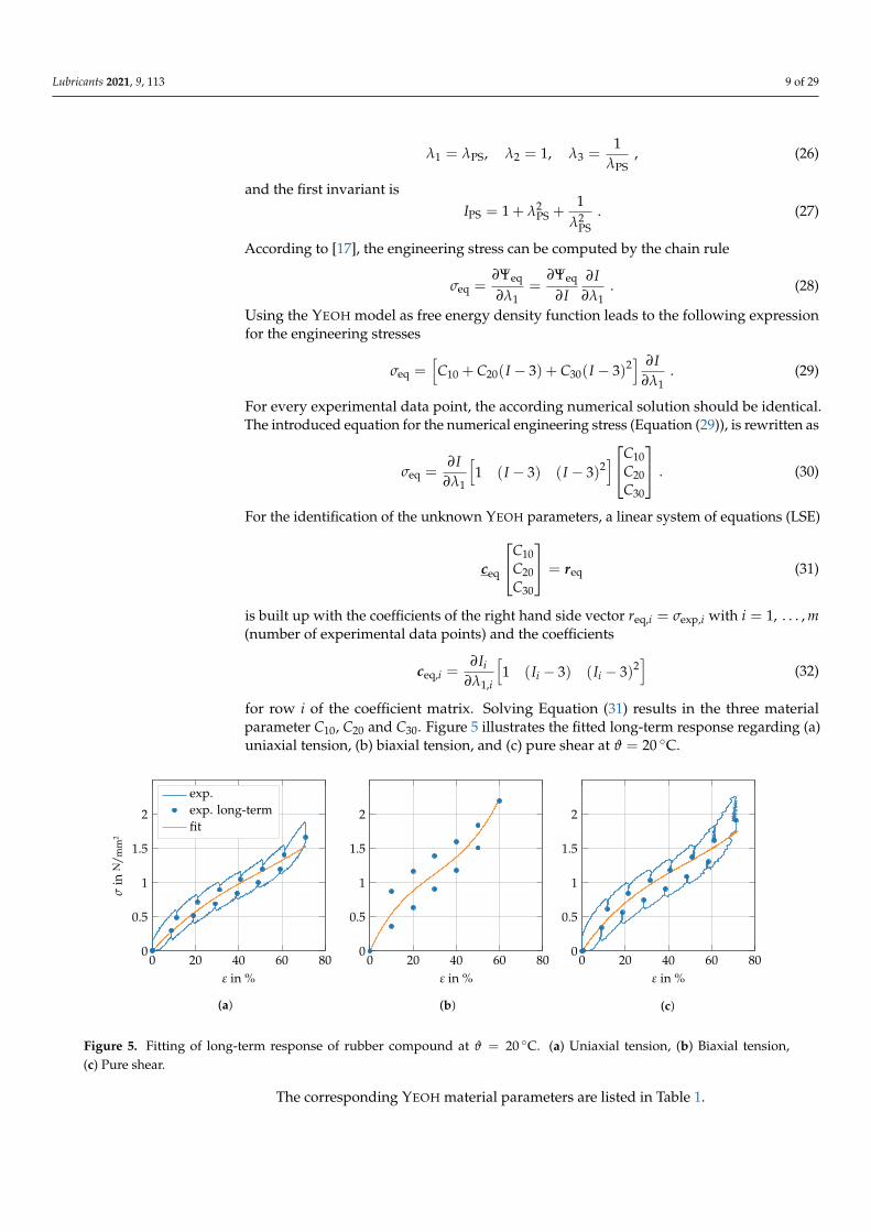
for row i of the coefficient matrix. Solving Equation (31) results in the three materialparameter C10, C20 and C30. Figure 5 illustrates the fitted long-term response regarding (a)uniaxial tension, (b) biaxial tension, and (c) pure shear at ϑ = 20 ◦C.Version November 5, 2021 submitted to Lubricants 9 of 28

0 20 40 60 800

1

2

0.5

1.5

ε in %

σin

N/m

m2

exp.exp. long-termfit

(a)

0 20 40 60 800

1

2

0.5

1.5

ε in %

(b)

0 20 40 60 800

1

2

0.5

1.5

ε in %

(c)

Figure 5. Fitting of long-term response of rubber compound at ϑ = 20 ◦C

Table 1. YEOH material parameters.

C10 C20 C30

0.57935 N/mm2 −0.04953 N/mm2 0.02483 N/mm2

According to [17], the engineering stress can be computed by the chain rule

σeq =∂Ψeq

∂λ1=

∂Ψeq

∂I∂I

∂λ1. (28)

Using the YEOH model as free energy density function leads to the following expression for theengineering stresses

σeq =[C10 + C20 (I − 3) + C30 (I − 3)2

] ∂I∂λ1

. (29)

For every experimental data point, the according numerical solution should be identical. Theintroduced equation for the numerical engineering stress (Equation (29)), is rewritten as

σeq =∂I

∂λ1

[1 (I − 3) (I − 3)2

]

C10

C20

C30

. (30)

For the identification of the unknown YEOH parameters, a linear system of equations (LSE)

ceq

C10

C20

C30

= req (31)

is built up with the coefficients of the right hand side vector req,i = σexp,i with i = 1, . . . , m (number ofexperimental data points) and the coefficients

ceq,i =∂Ii

∂λ1,i

[1 (Ii − 3) (Ii − 3)2

](32)

for row i of the coefficient matrix. Solving Equation (31) results in the three material parameter C10,138

C20 and C30. Figure 5 illustrates the fitted long-term response regarding (a) uniaxial tension, (b) biaxial139

tension and (c) pure shear at ϑ = 20 ◦C. The corresponding YEOH material parameters are listed in140

Table 1.141

Figure 5. Fitting of long-term response of rubber compound at ϑ = 20 ◦C. (a) Uniaxial tension, (b) Biaxial tension,(c) Pure shear.

The corresponding YEOH material parameters are listed in Table 1.

Lubricants 2021, 9, 113 10 of 29

Table 1. YEOH material parameters.

C10 C20 C30

0.57935 N/mm2 −0.04953 N/mm2 0.02483 N/mm2

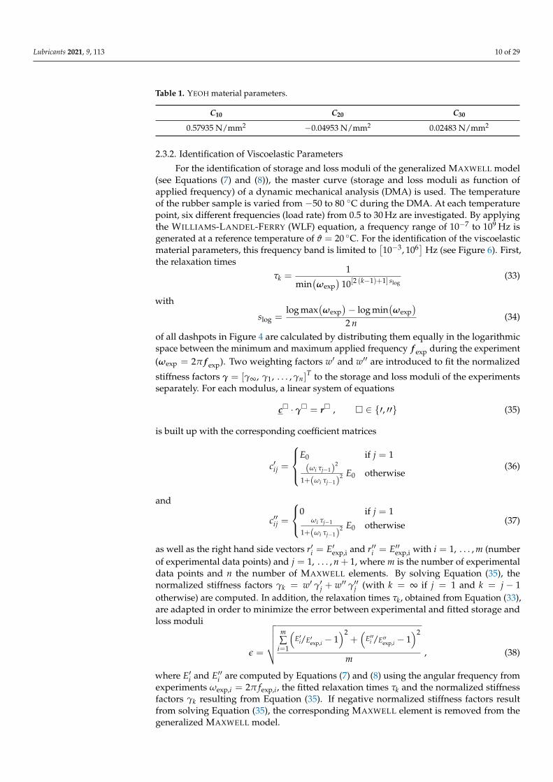
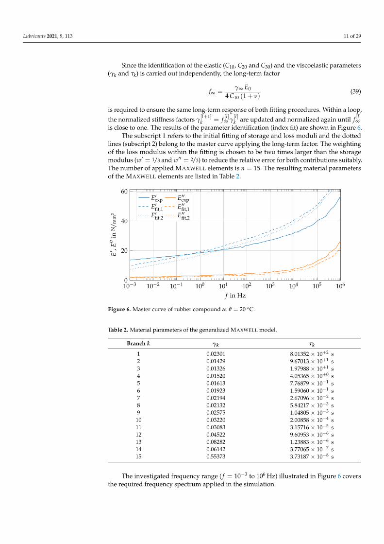
2.3.2. Identification of Viscoelastic Parameters

For the identification of storage and loss moduli of the generalized MAXWELL model(see Equations (7) and (8)), the master curve (storage and loss moduli as function ofapplied frequency) of a dynamic mechanical analysis (DMA) is used. The temperatureof the rubber sample is varied from −50 to 80 ◦C during the DMA. At each temperaturepoint, six different frequencies (load rate) from 0.5 to 30 Hz are investigated. By applyingthe WILLIAMS-LANDEL-FERRY (WLF) equation, a frequency range of 10−7 to 109 Hz isgenerated at a reference temperature of ϑ = 20 ◦C. For the identification of the viscoelasticmaterial parameters, this frequency band is limited to

[10−3, 106] Hz (see Figure 6). First,

the relaxation timesτk =

1

min(ωexp

)10[2 (k−1)+1] slog

(33)

with

slog =log max

(ωexp

)− log min

(ωexp

)

2 n(34)

of all dashpots in Figure 4 are calculated by distributing them equally in the logarithmicspace between the minimum and maximum applied frequency f exp during the experiment(ωexp = 2π f exp). Two weighting factors w′ and w′′ are introduced to fit the normalized

stiffness factors γ = [γ∞, γ1, . . . , γn]T to the storage and loss moduli of the experiments

separately. For each modulus, a linear system of equations

c� · γ� = r� , � ∈ {′, ′′} (35)

is built up with the corresponding coefficient matrices

c′ij =

E0 if j = 1(ωi τj−1)

2

1+(ωi τj−1)2 E0 otherwise

(36)

and

c′′ij =

0 if j = 1ωi τj−1

1+(ωi τj−1)2 E0 otherwise (37)

as well as the right hand side vectors r′i = E′exp,i and r′′i = E′′exp,i with i = 1, . . . , m (numberof experimental data points) and j = 1, . . . , n + 1, where m is the number of experimentaldata points and n the number of MAXWELL elements. By solving Equation (35), thenormalized stiffness factors γk = w′ γ′j + w′′ γ′′j (with k = ∞ if j = 1 and k = j − 1otherwise) are computed. In addition, the relaxation times τk, obtained from Equation (33),are adapted in order to minimize the error between experimental and fitted storage andloss moduli

ε =

√√√√√m∑

i=1

(E′i/E′exp,i − 1

)2+(

E′′i /E′′exp,i − 1)2

m, (38)

where E′i and E′′i are computed by Equations (7) and (8) using the angular frequency fromexperiments ωexp,i = 2π fexp,i, the fitted relaxation times τk and the normalized stiffnessfactors γk resulting from Equation (35). If negative normalized stiffness factors resultfrom solving Equation (35), the corresponding MAXWELL element is removed from thegeneralized MAXWELL model.

Lubricants 2021, 9, 113 11 of 29

Since the identification of the elastic (C10, C20 and C30) and the viscoelastic parameters(γk and τk) is carried out independently, the long-term factor

f∞ =γ∞ E0

4 C10 (1 + ν)(39)

is required to ensure the same long-term response of both fitting procedures. Within a loop,the normalized stiffness factors γ

[l+1]k = f [l]∞ γ

[l]k are updated and normalized again until f [l]∞

is close to one. The results of the parameter identification (index fit) are shown in Figure 6.The subscript 1 refers to the initial fitting of storage and loss moduli and the dotted

lines (subscript 2) belong to the master curve applying the long-term factor. The weightingof the loss modulus within the fitting is chosen to be two times larger than the storagemodulus (w′ = 1/3 and w′′ = 2/3) to reduce the relative error for both contributions suitably.The number of applied MAXWELL elements is n = 15. The resulting material parametersof the MAXWELL elements are listed in Table 2.

10−3 10−2 10−1 100 101 102 103 104 105 1060

20

40

60

f in Hz

E′ ,

E′′

inN

/mm

2

E′exp E′′expE′fit,1 E′′fit,1E′fit,2 E′′fit,2

Figure 6. Master curve of rubber compound at ϑ = 20 ◦C.

Table 2. Material parameters of the generalized MAXWELL model.

Branch k γk τk

1 0.02301 8.01352 × 10+2 s2 0.01429 9.67013 × 10+1 s3 0.01326 1.97988 × 10+1 s4 0.01520 4.05365 × 10+0 s5 0.01613 7.76879 × 10−1 s6 0.01923 1.59060 × 10−1 s7 0.02194 2.67096 × 10−2 s8 0.02132 5.84217 × 10−3 s9 0.02575 1.04805 × 10−3 s10 0.03220 2.00858 × 10−4 s11 0.03083 3.15716 × 10−5 s12 0.04522 9.60953 × 10−6 s13 0.08282 1.23883 × 10−6 s14 0.06142 3.77065 × 10−7 s15 0.55373 3.73187 × 10−8 s

The investigated frequency range ( f = 10−3 to 106 Hz) illustrated in Figure 6 coversthe required frequency spectrum applied in the simulation.

Lubricants 2021, 9, 113 12 of 29

2.4. Wear Model

Wear is a consequence of friction between contact partners [18]. In this work, a combi-nation of ARCHARD’s wear model (see [19]) also known as REYE-ARCHARD-KHRUSHCHOV

wear law and the abrasion law by SCHALLAMACH (see [20]) are applied. In ARCHARD’swear model, wear volume

Vw,RAK =kH

FN L (40)

is a result of normal contact forces FN , sliding distance L, material hardness H, and wearcoefficient k. In contrast, SCHALLAMACH directly links the frictional energy (simplified asµ FN L) to the resulting wear volume

Vw,S = γ µFN L , (41)

where γ represents the rate of abrasion per unit rate of energy dissipation. In recentpublications (e.g., [3,4,21]), the abrasion rate law

Vw = kw · D aws (42)

with frictional dissipation rate or frictional energy rate Ds, wear coefficient kw and wearexponent aw is an extension of the approaches of ARCHARD and SCHALLAMACH. The wearmodel implemented in this work is based on Equation (42), where the frictional energy rate

Ds =∫

A

tT vT dA (43)

is the integral of contact shear stresses tT and sliding velocity vector vT over the area of thecontact surface A. The shear stresses

tT = µ pN ϕigT‖ gT ‖

(44)

are calculated by the coefficient of friction µ, the normal pressure pN ≥ 0, the contact slipvector gT and the function φi, that describes the transition from sticking to sliding. In [22],an overview of different regularization functions, e.g.

ϕ1 =

{ ‖ gT ‖gcrit

if ‖ gT ‖ < gcrit

1 otherwise(45)

or

ϕ2 = tanh(‖ gT ‖

ε

)(46)

are given. If the hyperbolic tangent regularization ϕ2 (Equation (46)) is applied, thetransition region (sticking to sliding) is differentiable, which is shown in Figure 7.

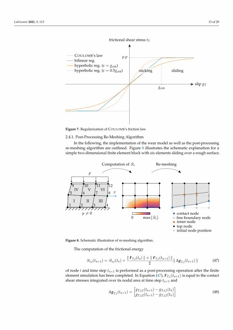
Lubricants 2021, 9, 113 13 of 29

gcrit

µ p

slidingsticking

slip gT

frictional shear stress tT

COULOMB’s lawbilinear reg.hyperbolic reg. (ε = gcrit)hyperbolic reg. (ε = 0.5gcrit)

Figure 7. Regularization of COULOMB’s friction law.

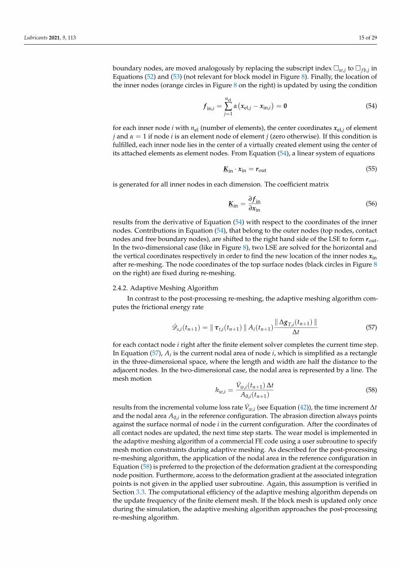
2.4.1. Post-Processing Re-Meshing Algorithm

In the following, the implementation of the wear model as well as the post-processingre-meshing algorithm are outlined. Figure 8 illustrates the schematic explanation for asimple two-dimensional finite element block with six elements sliding over a rough surface.

free boundary node

v

µ 6= 0

p

Computation of Ds

contact node

Re-meshing

inner nodetop node

0 max(Ds)

initial node position

1 2 3 4

5 6 7 8

9 10 11 12

I II III

IV V VI

Figure 8. Schematic illustration of re-meshing algorithm.

The computation of the frictional energy

Ds,i(tn+1) = Ds,i(tn) +‖ FT,i(tn) ‖+ ‖ FT,i(tn+1) ‖

2‖∆gT,i(tn+1) ‖ (47)

of node i and time step tn+1 is performed as a post-processing operation after the finiteelement simulation has been completed. In Equation (47), FT,i(tn+1) is equal to the contactshear stresses integrated over its nodal area at time step tn+1 and

∆gT,i(tn+1) =

[gT,i,1(tn+1)− gT,i,1(tn)gT,i,2(tn+1)− gT,i,2(tn)

](48)

Lubricants 2021, 9, 113 14 of 29

relates to the change in contact slip between time step tn and tn+1 of the same node. Acontour plot of the frictional energy rate

Ds,i(tn+1) =Ds,i(tn+1)−Ds,i(tn)

∆t(49)

of the block model example is shown in the center image of Figure 8. In Equation (49), ∆tis defined by tn+1 − tn. After the frictional energy rate computation has been completed,re-meshing starts. The re-meshing algorithm contains three procedures: moving contactnodes, free boundary nodes, and inner nodes (see right image in Figure 8). The wear height

hw,i(tn+1) = hw,i(tn) +Vw,i(tn+1)−Vw,i(tn)

A0,i(tn+1)(50)

is computed cumulatively out of the incremental wear volume resulting from Equation (42)and the nodal area in the reference configuration (see explanation below). The new positionof each contact node xw,i = Xw,i + uw,i is defined by

uw,i =nt−1

∑n=1−[hw,i(tn+1)− hw,i(tn)]ni(tn+1) , (51)

where nt coincides with the number of time steps and ni is the unit-length normal vector(‖ ni ‖ = 1) of node i in the current configuration. ni is obtained by averaging the normalvectors of all element faces that are connected to node i and belong to the contact surface.To apply the abrasion vector to the nodal coordinates in the reference configuration, uw,ishould be left multiplied by the inverse of the deformation gradient at node i, if the nodalarea in the current configuration is used in Equation (50). However, the deformationgradient is only defined at the integration points within the element. A projection to theelement nodes by shape functions increases the computational costs significantly and leadsto an unknown error due to averaging at nodes, which are connected to multiple elements.For this reason, the nodal area in the reference configuration is considered instead inEquation (50). This assumption is verified in Section 3.3. Since the computation of thewear height in Equation (50) is approximated by using the nodal area, an internal iterationminimizes the difference between the node based wear volume Vw,i and the resulting wearvolume on the element level, taking the new position of the contact nodes into account. Forthis purpose, each displacement vector uw,i is multiplied by an abrasion factor fw,i with

f [1]w,i = 1 for the first iteration. By comparing nodal and elemental wear, this factor varies inthe range of 1± fw,max with fw,max < 1 for each node separately. After the new positionof the contact nodes (blue circles in Figure 8 on the right) is known, the boundary nodes,which belong neither to the top nor the contact nodes, are moved as follows. First, thepossible moving directions (only along element edges) of each free boundary node i (whitecircles in Figure 8 on the right), which is attached to a contact node j, are identified. Thedecisive direction is detected by computing the dot products

dfb,k =(Xfb,i − Xw,j

)· (Xk − Xfb,i) (52)

of vector Xfb,i − Xw,j (contact node j to free boundary node i) and vector Xk − Xfb,i (freeboundary node i to connected element edge node k) with k 6= j. Node k = argmax dfbdefines the resulting moving direction of free boundary node i, which is moved by

ufb,i =‖ uw,j ‖ dfb,k

∆Xfb,i

∆Xfb,i +dfb,k

∆Xfb,i

Xk − Xfb,i

‖Xk − Xfb,i ‖(53)

with ∆Xfb,i = ‖Xfb,i − Xw,j ‖ to get its new position xfb,i = Xfb,i + ufb,i. Subsequently,the next row of free boundary nodes, which are connected to the previously modified

Lubricants 2021, 9, 113 15 of 29

boundary nodes, are moved analogously by replacing the subscript index �w,j to � f b,j inEquations (52) and (53) (not relevant for block model in Figure 8). Finally, the location ofthe inner nodes (orange circles in Figure 8 on the right) is updated by using the condition

f in,i =nel

∑j=1

α(xel,j − xin,i

)= 0 (54)

for each inner node i with nel (number of elements), the center coordinates xel,j of elementj and α = 1 if node i is an element node of element j (zero otherwise). If this condition isfulfilled, each inner node lies in the center of a virtually created element using the center ofits attached elements as element nodes. From Equation (54), a linear system of equations

Kin · xin = rout (55)

is generated for all inner nodes in each dimension. The coefficient matrix

Kin =∂ f in∂xin

(56)

results from the derivative of Equation (54) with respect to the coordinates of the innernodes. Contributions in Equation (54), that belong to the outer nodes (top nodes, contactnodes and free boundary nodes), are shifted to the right hand side of the LSE to form rout.In the two-dimensional case (like in Figure 8), two LSE are solved for the horizontal andthe vertical coordinates respectively in order to find the new location of the inner nodes xinafter re-meshing. The node coordinates of the top surface nodes (black circles in Figure 8on the right) are fixed during re-meshing.

2.4.2. Adaptive Meshing Algorithm

In contrast to the post-processing re-meshing, the adaptive meshing algorithm com-putes the frictional energy rate

Ds,i(tn+1) = ‖ τt,i(tn+1) ‖ Ai(tn+1)‖∆gT,i(tn+1) ‖

∆t(57)

for each contact node i right after the finite element solver completes the current time step.In Equation (57), Ai is the current nodal area of node i, which is simplified as a rectanglein the three-dimensional space, where the length and width are half the distance to theadjacent nodes. In the two-dimensional case, the nodal area is represented by a line. Themesh motion

hw,i =Vw,i(tn+1)∆t

A0,i(tn+1)(58)

results from the incremental volume loss rate Vw,i (see Equation (42)), the time increment ∆tand the nodal area A0,i in the reference configuration. The abrasion direction always pointsagainst the surface normal of node i in the current configuration. After the coordinates ofall contact nodes are updated, the next time step starts. The wear model is implemented inthe adaptive meshing algorithm of a commercial FE code using a user subroutine to specifymesh motion constraints during adaptive meshing. As described for the post-processingre-meshing algorithm, the application of the nodal area in the reference configuration inEquation (58) is preferred to the projection of the deformation gradient at the correspondingnode position. Furthermore, access to the deformation gradient at the associated integrationpoints is not given in the applied user subroutine. Again, this assumption is verified inSection 3.3. The computational efficiency of the adaptive meshing algorithm depends onthe update frequency of the finite element mesh. If the block mesh is updated only onceduring the simulation, the adaptive meshing algorithm approaches the post-processingre-meshing algorithm.

Lubricants 2021, 9, 113 16 of 29

2.5. Image Processing and Mesh Generation2.5.1. Image Processing

The profiles of the rubber samples are recorded by a camera after the run-in phase(pre-conditioning) and after the friction/wear test (see Section 2.1). These photographsof the rubber profiles are used to identify the boundary shape of the pre-conditioned aswell as the worn rubber blocks. An image processing procedure is developed by applyingdifferent modules of the scikit-image package in Python [23]. In Figure 9, the work flow isillustrated exemplary for the pre-conditioned block at p = 1.2 N/mm2 and v = 100 mm/s.

(a) (b)

(c) (d)

(e) (f)

Figure 9. Image processing at p = 1.2 N/mm2 and v = 100 mm/s. (a) Original, (b) Color inversion, (c) Backgrounddeletion, (d) SOBEL filter, (e) GAUSSian filter, (f) Contour identification.

First, the contrast of the image is adjusted by histogram equalization (see [24]) toimprove the output during the color space inversion in Figure 9b. As result, the darkyellowish background in Figure 9a changes to different shades of blue. In the next step, thebackground can be removed by defining a minimal blue contribution from the red-green-blue (RGB) color model. In the digital RGB color model, each color channel is assigneda value between 0 and 255. Applying a normalized minimal blue contribution of 0.85(0.85 × 255 ≈ 217) leads to the outcome presented in Figure 9c. In the following step, theSOBEL filter (also called SOBEL-FELDMAN operator) is applied in order to detect the blockedges [25]. For a suitable presentation in Figure 9d, the output of the SOBEL filter is visualizedin the inverted gray-scale. Furthermore, a flood tool is used to identify connected pointswithin a tolerance of the seed value starting from a specific seed point. To apply a multi-dimensional GAUSSian filter, which enhances the gray gradients at the edges, the originalphoto is transferred into gray scale. The color white is assigned to the connected points fromthe flood tool. Figure 9e shows the results using a tolerance value for the flood tool of 0.01 anda standard deviation for the GAUSSian kernel of 0.9. Finally, the block contour is identified

Lubricants 2021, 9, 113 17 of 29

by the marching-squares method to compute an iso-valued contour of a two-dimensionalarray [26]. The block contour for a level value of 0.9 (0→ black, 1→white).

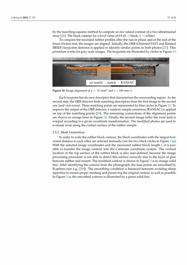
To compare the recorded rubber profiles after the run-in phase and at the end of thelinear friction test, the images are aligned. Initially, the ORB (Oriented FAST and RotatedBRIEF) keypoints detector is applied to identify similar points in both photos [27]. Thisprocedure works for gray-scale images. The keypoints are illustrated by circles in Figure 10.

no match match RANSAC

Figure 10. Image alignment at p = N/mm2 and v = 100 mm/s.

Each keypoint has its own descriptor that characterizes the surrounding region. As thesecond step, the ORB detector finds matching descriptors from the first image in the secondone (and vice-versa). These matching points are represented by blue circles in Figure 10. Toimprove the output of the ORB detector, a random sample consensus (RANSAC) is appliedon top of the matching points [28]. The remaining connections of the alignment pointsare shown as orange lines in Figure 10. Finally, the second image (after the wear test) iswarped according to a given coordinate transformation. The modified photos are used toevaluate wear along the contact surface of the rubber sample.

2.5.2. Mesh Generation

In order to scale the rubber block contour, the block coordinates with the largest hori-zontal distance to each other are selected manually (see the two black circles in Figure 11a).With the selected image coordinates and the measured rubber block length l, it is pos-sible to transfer the image contour into the Cartesian coordinate system. The verticallocation of the top surface of the rubber block is also user-defined, because the imageprocessing procedure is not able to detect this surface correctly due to the layer of gluebetween rubber and mount. The modified contour is shown in Figure 11a as orange solidline. After identifying the contour from the photograph, the data points are smoothed byB-splines (see e.g., [29]). The smoothing condition is balanced between avoiding sharpasperities to ensure proper meshing and preserving the original contour as well as possible.In Figure 11a, the smoothed contour is illustrated by a green solid line.

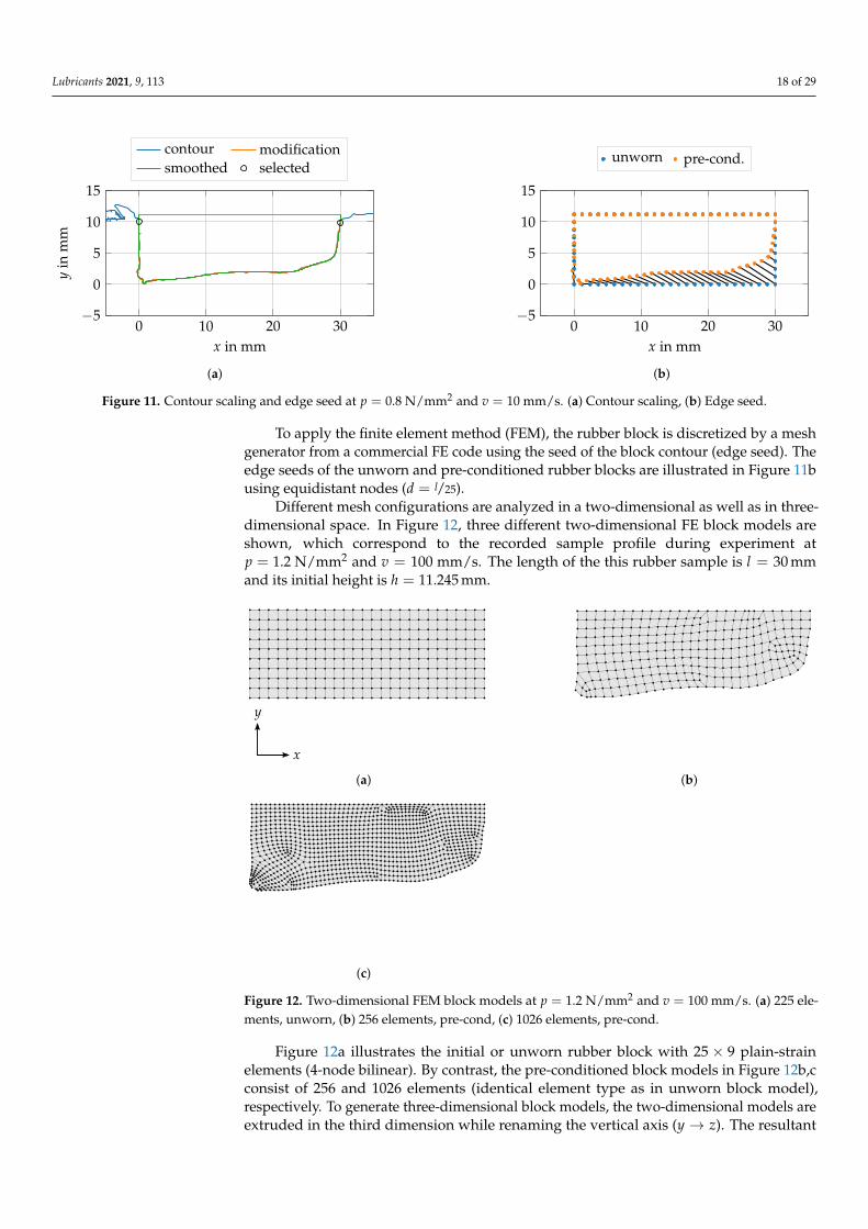
Lubricants 2021, 9, 113 18 of 29

0 10 20 30−5

0

5

10

15

x in mm

yin

mm

contour modificationsmoothed selected

(a)

0 10 20 30−5

0

5

10

15

x in mm

unworn pre-cond.

(b)

Figure 11. Contour scaling and edge seed at p = 0.8 N/mm2 and v = 10 mm/s. (a) Contour scaling, (b) Edge seed.

To apply the finite element method (FEM), the rubber block is discretized by a meshgenerator from a commercial FE code using the seed of the block contour (edge seed). Theedge seeds of the unworn and pre-conditioned rubber blocks are illustrated in Figure 11busing equidistant nodes (d = l/25).

Different mesh configurations are analyzed in a two-dimensional as well as in three-dimensional space. In Figure 12, three different two-dimensional FE block models areshown, which correspond to the recorded sample profile during experiment atp = 1.2 N/mm2 and v = 100 mm/s. The length of the this rubber sample is l = 30 mmand its initial height is h = 11.245 mm.

x

y

(a) (b)

(c)

Figure 12. Two-dimensional FEM block models at p = 1.2 N/mm2 and v = 100 mm/s. (a) 225 ele-ments, unworn, (b) 256 elements, pre-cond, (c) 1026 elements, pre-cond.

Figure 12a illustrates the initial or unworn rubber block with 25 × 9 plain-strainelements (4-node bilinear). By contrast, the pre-conditioned block models in Figure 12b,cconsist of 256 and 1026 elements (identical element type as in unworn block model),respectively. To generate three-dimensional block models, the two-dimensional models areextruded in the third dimension while renaming the vertical axis (y → z). The resultant

Lubricants 2021, 9, 113 19 of 29

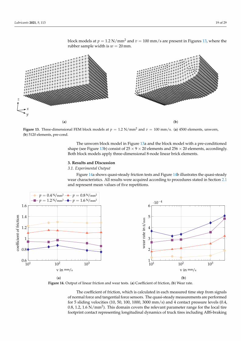
block models at p = 1.2 N/mm2 and v = 100 mm/s are present in Figures 13, where therubber sample width is w = 20 mm.

xy

z

(a) (b)

Figure 13. Three-dimensional FEM block models at p = 1.2 N/mm2 and v = 100 mm/s. (a) 4500 elements, unworn,(b) 5120 elements, pre-cond.

The unworn block model in Figure 13a and the block model with a pre-conditionedshape (see Figure 13b) consist of 25× 9× 20 elements and 256× 20 elements, accordingly.Both block models apply three-dimensional 8-node linear brick elements.

3. Results and Discussion3.1. Experimental Output

Figure 14a shows quasi-steady friction tests and Figure 14b illustrates the quasi-steadywear characteristics. All results were acquired according to procedures stated in Section 2.1and represent mean values of five repetitions.

101 102 1030.6

0.8

1

1.2

1.4

1.6

v in mm/s

coef

ficie

ntof

fric

tion

p = 0.4 N/mm2 p = 0.8 N/mm2

p = 1.2 N/mm2 p = 1.6 N/mm2

(a)

101 102 1031

2

3

4

5

6·10−4

v in mm/s

wea

rra

tein

g /m

m

(b)Figure 14. Output of linear friction and wear tests. (a) Coefficient of friction, (b) Wear rate.

The coefficient of friction, which is calculated in each measured time step from signalsof normal force and tangential force sensors. The quasi-steady measurements are performedfor 5 sliding velocities (10, 50, 100, 1000, 3000 mm/s) and 4 contact pressure levels (0.4,0.8, 1.2, 1.6 N/mm2). This domain covers the relevant parameter range for the local tirefootprint contact representing longitudinal dynamics of truck tires including ABS-braking

Lubricants 2021, 9, 113 20 of 29

and acceleration. The coefficient of friction of the truck compound on sand paper is inthe range of 0.7 and 1.3, with a clearly decreasing trend over increasing contact pressure.This expected characteristics is a direct consequence of the real contact area of a compliantmaterial on a solid rough surface. Above a certain contact pressure, the contact area cannotgrow significantly, thus, the normal force is increasing but the transmissible tangentialforce is not. Hence, the coefficient of friction decreases. In terms of sliding velocity, thiscompound shows a relatively uniform friction level for each contact pressure stage.

The wear characteristics exhibit an increasing wear rate over both sliding velocity andcontact pressure. This shows the close relation between wear rate and frictional power inthe parameter range tested in the scope of this paper. The minimum at 50 mm/s for highpressure characteristics is not considered as statistically significant here. The high absolutelevel of wear (0.01 to 0.05 mg/mm) can be attributed to the strong abrasiveness of the sandpaper track and the strict surface cleaning routine. The monotonous properties of the wearcharacteristics without maxima underline the assumption that only one wear mechanismis dominant (see [5]).

3.2. Wear Parameter Identification

The wear parameters introduced in Equation (42) (see Section 2.4) are identified byusing the experimental output of the block tests described in Section 3.1. The frictionalenergy rate in the experiment

Ds,exp =µ pN A L

∆t(59)

considers the recorded friction coefficient µ, the normal pressure pN applied on the topside of the block (area A), the sliding distance L and the time period ∆t of each test. Theabrasion rate in terms of volume

Vw,exp =mw

ρ(60)

is computed by the mass loss rate (recorded mass difference divided by ∆t) and the densityof the applied rubber material ρ = 1.12 × 10−3 g/mm3.

To compare the abrasion rate from experiment and simulation, the averaged EU-CLIDean distance

D2,abs =

√1n

n

∑i=1

(Vw,exp,i − Vw,i

)2 (61)

is applied to calculate the mean absolute error between both quantities. In Equation (61), nrepresents the number of experimental data points. To obtain the relative error D2,rel, theterm

(Vw,exp,i − Vw,i

)2 in Equation (61) is divided by V2w,exp,i. An optimization tool identifies

the wear parameters kw and aw by minimizing the error value defined in Equation (61).Figure 15 shows the result of the fitting procedure in logarithmic space.

A linear as well as a non-linear correlation between frictional energy rate and abrasionrate are investigated. Table 3 lists all parameter combinations including the resultingcoefficient of determination

R2 = 1−

m∑

i=1

(Vw,exp,i − Vw,i

)2

m∑

i=1

(Vw,exp,i − Vw,exp

)2 , (62)

which indicate if the abrasion rate is predictable by the underlying wear model function.

Lubricants 2021, 9, 113 21 of 29

104 105 106100

101

102

103

Ds in Nmm/s

Vw

inm

m3 /s

0.4 N/mm2

0.8 N/mm2

1.2 N/mm2

1.6 N/mm2

10 mm/s

50 mm/s

100 mm/s

1000 mm/s

3000 mm/s

D2,abs, linearD2,rel, linearD2,abs, non-linearD2,rel, non-linear

Figure 15. Wear parameter identification.

Table 3. Wear parameters and associated coefficient of determination.

Parameter Linear (abs. Error) Linear (rel. Error) Non-Linear (abs. Error) Non-Linear (rel. Error)

kw in mm2/N 5.951×10−4 3.857×10−4 2.083×10−5 1.452×10−4

aw 1 1 1.234 1.089

R2 0.978 0.808 0.988 0.961

By using the relative error D2,rel, the wear model covers the entire range slidingvelocities of the experiments, especially the low frictional energy rates at low slidingvelocities. The corresponding coefficients of determination (see Table 3, Columns 3 and5) are lower in comparison to the R2 values using the absolute error D2,abs, becauseEquation (62) does not consider relative differences. The wear parameters in Table 3,Columns 3 and 5 are applied for the validation of the wear model in Section 3.3.

3.3. Wear Simulation and Comparison to Experiments3.3.1. Wear Simulation

To simulate the experiments introduced in Section 2.1 in a proper manner, the gener-ated FE block models described in Section 2.5 are applied within the different re-meshingalgorithms (see Section 2.4) using the wear model parameters in Table 3. The counter sur-face as well as the mount of the rubber sample are modeled as rigid bodies (see Figure 16).Previously performed simulations have shown that the application of the mount is re-quired to avoid unrealistic folding at top of the trailing edge of the rubber mesh during thesliding step.

surface

uy

Fy

vx counter surface

mount

µ

x

y

RP mount

RP counterrubber block

Figure 16. FE model setup.

Lubricants 2021, 9, 113 22 of 29

The augmented LAGRANGE method is used to enforce the contact constraints betweenthe rubber block model and the rigid body surfaces [30]. Frictionless contact is assumedbetween the mount and the rubber block. The friction coefficient at the counter surfaceis changing during the simulation depending on the current step in order to model bothsurfaces aluminum and sandpaper. Table 4 gives an overview of the simulation steps foreach test run.

Table 4. Steps of the FEM simulation.

Number Name Description BoundaryConditions

1 ContactCounter surface is lifted to ensure contactbetween rubber block and bottom rigidsurface

∆t = 10−2 suv = 1 mm

2 Loading Counter surface is pressed against rubberblock

∆t = 1 sFv = pN A

3 Ramping Counter surface is accelerated while frictionis continuously increased

∆t = va

vx = a tµ = µalu t

4 Sliding-on-aluminum

Counter surface is moving with constantspeed and aluminum based friction

∆t = Lalu− v22a

vvx = vµ = µalu

5 Sliding-on-sandpaper

Counter surface is moving with constantspeed and sandpaper based friction

∆t = Lspv

vx = vµ = µsp

Due to the glued connection between the mount and the top surface of the rubbersample in the experiment, all rubber block nodes located at the top surface are fixed duringthe entire simulation. To improve the convergence of the simulation, the counter surfaceis lifted vertically by uv = 1 mm to get into contact with the rubber block during the firststep. In the next step, the load Fv = pN A, where pN is the normal pressure (applied inexperiment) and A represents the area of the top surface of the rubber block, is applied invertical direction (positive y- and z-direction in 2D and 3D, respectively) at the referencepoint of the counter surface. In the two-dimensional case, A is equal to the length of theblock’s top surface. In Step 3, the counter surface is accelerated by a = 5 g = 49.05 m/s2

horizontally (negative x-direction) and an averaged friction coefficient for aluminumrecorded during the experiment is increased linearly. Subsequently, the counter surface ismoved constantly by the predefined velocity v. The sliding distance on the aluminum sheetLalu is determined in the experiment (see Section 2.1). The friction property is changingto the averaged coefficient of friction, which is observed on sandpaper instantaneously atthe beginning of the last step. The sliding distance Lsp corresponds to the elapsed slidingdistance on the linear friction tester within one run.

Due to friction, the substrate as well as the rubber block is warmed-up. Since thecoefficient of friction and the wear model are based on experimental data, friction as wellas wear features due to temperature change are considered in the simulation. Heating ofthe rubber block during sliding is initially neglected in the simulation, because on average(of all laboratory tests), the temperature at the bottom surface of the rubber block has beenchanged by approximately ∆ϑ = 12.2 ◦C. The maximum temperature increment, whichis recorded by the HiLiTe at p = 1.6 N/mm2 and v = 3000 mm/s, is ∆ϑ = 27.1 ◦C. Theinfluence of the temperature is part of future research using, e.g., a thermo-mechanicallycoupled block simulation and temperature-dependent parameters for the rubber material.After each test, the rubber sample is cooled down to ambient temperature (ϑ = 20 ◦C).

Lubricants 2021, 9, 113 23 of 29

If the post-processing re-meshing algorithm introduced in Section 2.4 is applied, thefrictional energy rate is computed at each contact node of the rubber block after completionof the simulation. As soon as new node coordinates are computed by the re-meshingalgorithm depending on the underlying wear model (linear or non-linear), the next testrun with the same program listed in Table 4 starts. If the adaptive meshing algorithmis used, the new coordinates of the contact nodes are already known at the end of thesimulation. Accordingly, only the location of the inner nodes and the free boundary nodes(see Figure 8) are updated by the re-meshing algorithm.

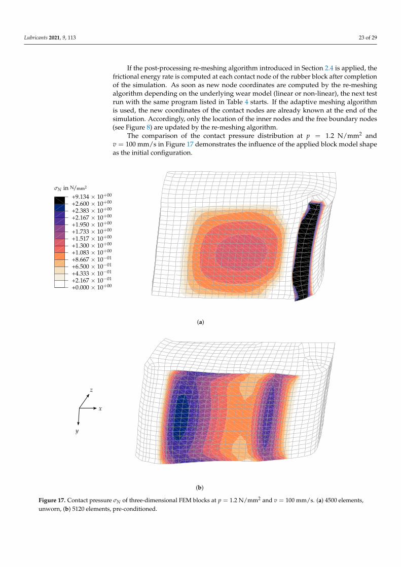
The comparison of the contact pressure distribution at p = 1.2 N/mm2 andv = 100 mm/s in Figure 17 demonstrates the influence of the applied block model shapeas the initial configuration.

σN in N/mm2

+0.000 × 10+00+2.167 × 10−01+4.333 × 10−01+6.500 × 10−01+8.667 × 10−01+1.083 × 10+00+1.300 × 10+00+1.517 × 10+00+1.733 × 10+00+1.950 × 10+00+2.167 × 10+00+2.383 × 10+00+2.600 × 10+00+9.134 × 10+00

(a)

x

z

y

(b)

Figure 17. Contact pressure σN of three-dimensional FEM blocks at p = 1.2 N/mm2 and v = 100 mm/s. (a) 4500 elements,unworn, (b) 5120 elements, pre-conditioned.

Lubricants 2021, 9, 113 24 of 29

The leading edge of the unworn block in Figure 17a folds immediately at the beginningof the sliding step, which causes the simulation to abort. The maximum contact pressureat the leading edge is approximately 10 times larger than contact pressure in the centerof the bottom surface and circa five times larger than the largest pressure value in thepre-conditioned block (see Figure 17b). This contact pressure concentration in combinationwith the abrasive sandpaper leads to uneven wear at the leading edge of the rubber block.The shape of the pre-conditioned sample results as a consequence of this phenomenon.

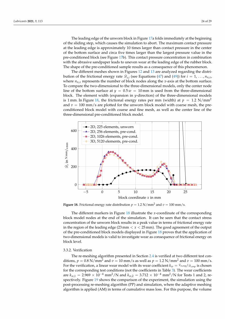
The different meshes shown in Figures 12 and 13 are analyzed regarding the distri-bution of the frictional energy rate Ds,i (see Equations (47) and (49)) for i = 1, . . . , nn,x,where nn,x represents the number of block nodes along the x-axis at the bottom surface.To compare the two-dimensional to the three-dimensional models, only the center nodeline of the bottom surface at y = 0.5 w = 10 mm is used from the three-dimensionalblock. The element width (expansion in y-direction) of the three-dimensional modelsis 1 mm. In Figure 18, the frictional energy rates per mm (width) at p = 1.2 N/mm2

and v = 100 mm/s are plotted for the unworn block model with coarse mesh, the pre-conditioned block model with coarse and fine mesh, as well as the center line of thethree-dimensional pre-conditioned block model.

−5 0 5 10 15 20 25

0

200

400

600

block coordinate x in mm

Ds

inN

mm

/sm

m

2D, 225 elements, unworn2D, 256 elements, pre-cond.2D, 1026 elements, pre-cond.3D, 5120 elements, pre-cond.

Figure 18. Frictional energy rate distribution p = 1.2 N/mm2 and v = 100 mm/s.

The different markers in Figure 18 illustrate the x-coordinate of the correspondingblock model nodes at the end of the simulation. It can be seen that the contact stressconcentration of the unworn block results in a peak value in terms of frictional energy ratein the region of the leading edge (23 mm < x < 25 mm). The good agreement of the outputof the pre-conditioned block models displayed in Figure 18 proves that the application oftwo-dimensional models is valid to investigate wear as consequence of frictional energy onblock level.

3.3.2. Verification

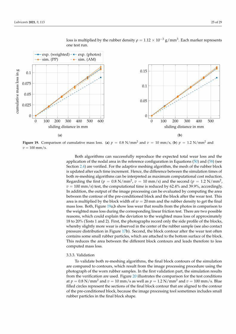
The re-meshing algorithm presented in Section 2.4 is verified at two different test con-ditions, p = 0.8 N/mm2 and v = 10 mm/s as well as p = 1.2 N/mm2 and v = 100 mm/s.For the verification, a linear wear model with its wear coefficient kw = Vw,exp/Ds,exp is chosenfor the corresponding test conditions (not the coefficients in Table 3). The wear coefficientsare kw,1 = 2.969 × 10−4 mm2/N and kw,2 = 3.712 × 10−4 mm2/N for Tests 1 and 2, re-spectively. Figure 19 shows the comparison of the experiment, the simulation using thepost-processing re-meshing algorithm (PP) and simulation, where the adaptive meshingalgorithm is applied (AM) in terms of cumulative mass loss. For this purpose, the volume

Lubricants 2021, 9, 113 25 of 29

loss is multiplied by the rubber density ρ = 1.12 × 10−3 g/mm3. Each marker representsone test run.

0 100 200 300 400 500 6000

0.05

0.1

0.025

0.075

sliding distance in mm

cum

ulat

ive

mas

slo

ssin

g

exp. (weighted) exp. (photos)sim. (PP) sim. (AM)

(a)

0 100 200 300 400 5000

0.05

0.1

0.15

sliding distance in mm

(b)

Figure 19. Comparison of cumulative mass loss. (a) p = 0.8 N/mm2 and v = 10 mm/s, (b) p = 1.2 N/mm2 andv = 100 mm/s.

Both algorithms can successfully reproduce the expected total wear loss and theapplication of the nodal area in the reference configuration in Equations (50) and (58) (seeSection 2.4) are verified. For the adaptive meshing algorithm, the mesh of the rubber blockis updated after each time increment. Hence, the difference between the simulation times ofboth re-meshing algorithms can be interpreted as maximum computational cost reduction.Regarding the first (p = 0.8 N/mm2, v = 10 mm/s) and the second (p = 1.2 N/mm2,v = 100 mm/s) test, the computational time is reduced by 62.4% and 39.9%, accordingly.In addition, the output of the image processing can be evaluated by computing the areabetween the contour of the pre-conditioned block and the block after the wear test. Thisarea is multiplied by the block width of w = 20 mm and the rubber density to get the finalmass loss. Both, Figure 19a,b show less wear that results from the photos in comparison tothe weighted mass loss during the corresponding linear friction test. There are two possiblereasons, which could explain the deviation to the weighted mass loss of approximately18 to 20% (Tests 1 and 2). First, the photographs record only the side profile of the blocks,whereby slightly more wear is observed in the center of the rubber sample (see also contactpressure distribution in Figure 17b). Second, the block contour after the wear test oftencontains some small rubber particles, which are attached to the bottom surface of the block.This reduces the area between the different block contours and leads therefore to lesscomputed mass loss.

3.3.3. Validation

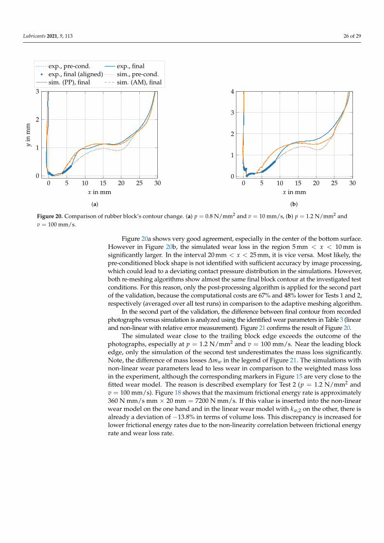
To validate both re-meshing algorithms, the final block contours of the simulationare compared to contours, which result from the image processing procedure using thephotograph of the worn rubber samples. In the first validation part, the simulation resultsfrom the verification are used. Figure 20 illustrates the comparison for the test conditionsat p = 0.8 N/mm2 and v = 10 mm/s as well as p = 1.2 N/mm2 and v = 100 mm/s. Bluefilled circles represent the sections of the final block contour that are aligned to the contourof the pre-conditioned block, because the image processing tool sometimes includes smallrubber particles in the final block shape.

Lubricants 2021, 9, 113 26 of 29

0 5 10 15 20 25 300

1

2

3

x in mm

yin

mm

exp., pre-cond. exp., finalexp., final (aligned) sim., pre-cond.sim. (PP), final sim. (AM), final

(a)

0 5 10 15 20 25 300

1

2

3

4

x in mm

(b)

Figure 20. Comparison of rubber block’s contour change. (a) p = 0.8 N/mm2 and v = 10 mm/s, (b) p = 1.2 N/mm2 andv = 100 mm/s.

Figure 20a shows very good agreement, especially in the center of the bottom surface.However in Figure 20b, the simulated wear loss in the region 5 mm < x < 10 mm issignificantly larger. In the interval 20 mm < x < 25 mm, it is vice versa. Most likely, thepre-conditioned block shape is not identified with sufficient accuracy by image processing,which could lead to a deviating contact pressure distribution in the simulations. However,both re-meshing algorithms show almost the same final block contour at the investigated testconditions. For this reason, only the post-processing algorithm is applied for the second partof the validation, because the computational costs are 67% and 48% lower for Tests 1 and 2,respectively (averaged over all test runs) in comparison to the adaptive meshing algorithm.

In the second part of the validation, the difference between final contour from recordedphotographs versus simulation is analyzed using the identified wear parameters in Table 3 (linearand non-linear with relative error measurement). Figure 21 confirms the result of Figure 20.

The simulated wear close to the trailing block edge exceeds the outcome of thephotographs, especially at p = 1.2 N/mm2 and v = 100 mm/s. Near the leading blockedge, only the simulation of the second test underestimates the mass loss significantly.Note, the difference of mass losses ∆mw in the legend of Figure 21. The simulations withnon-linear wear parameters lead to less wear in comparison to the weighted mass lossin the experiment, although the corresponding markers in Figure 15 are very close to thefitted wear model. The reason is described exemplary for Test 2 (p = 1.2 N/mm2 andv = 100 mm/s). Figure 18 shows that the maximum frictional energy rate is approximately360 N mm/s mm × 20 mm = 7200 N mm/s. If this value is inserted into the non-linearwear model on the one hand and in the linear wear model with kw,2 on the other, there isalready a deviation of −13.8% in terms of volume loss. This discrepancy is increased forlower frictional energy rates due to the non-linearity correlation between frictional energyrate and wear loss rate.

Lubricants 2021, 9, 113 27 of 29

0 2 4 6 8 10 12 14 16 18 20 22 24 26 28−0.6

−0.4

−0.2

0

0.2

0.4

0.6

x in mm

∆y

inm

mlinear, v = 10 mm/s, p = 0.8 N/mm2, ∆mw = 34.9 %non-linear, v = 10 mm/s, p = 0.8 N/mm2, ∆mw = −20.0 %linear, v = 100 mm/s, p = 1.2 N/mm2, ∆mw = 7.5 %non-linear, v = 100 mm/s, p = 1.2 N/mm2, ∆mw = −21.7 %

Figure 21. Final block contour difference between experiment and simulation.

4. Conclusions

A wear model based on frictional energy rate is proposed in this work. Two differentre-meshing algorithms are implemented in order to update the block geometry due to wear.Linear friction and wear tests on block level at different loads and sliding velocities areperformed to identify the friction features and wear model parameters. The rubber blocksamples are run-in (pre-conditioning) until a constant wear rate is observed during thelaboratory tests. By recording the change of the longitudinal rubber profile, it is possibleto validate the re-meshing algorithm. For this purpose, an image processing tool detectsthe block shape after pre-conditioning and after the wear test to generate the FE mesh andcompare the worn block geometry with the wear simulation results, respectively.

The quality of the photos, especially the lighting conditions, influences the reliabilityof the image processing tool significantly. In order to compare the block shape fromexperiments with the wear simulations, the accuracy of the image processing tool shouldbe in 0.01 mm range. This could not be achieved for all wear tests, because the contrastbetween background and rubber sample varies within the photo due to non-centralizedexposure to light. However, the application of the pre-conditioned block shape is requiredto obtain a reasonable contact pressure distribution at the bottom surface of the finiteelement block (see Figure 17). Due to the rate-dependent material properties of rubber, it isnecessary to model the entire process of the wear test, starting from rubber compressionand acceleration phase on aluminum. A comparison between two- and three-dimensionalblock models with respect to the evolution of frictional energy proves the usability of two-dimensional block models for this type of wear analysis to reduce the computational costs(see Figure 18). A verification study of the linear wear model in combination with bothre-meshing algorithms confirms the correct implementation by comparing the resultingmass loss of the wear test with the simulation (see Figure 19). In case of steady-state frictionand wear during (short-term) sliding, it is recommended to consider a post-processing re-meshing algorithm to update the finite element mesh in order to reduce the computationalcosts. In general, the worn block model geometry after the wear simulation is in goodagreement with the output of the image processing tool. Note that the results of the blockshape comparison strongly depends on the photo quality and image processing parameters.

Lubricants 2021, 9, 113 28 of 29

Author Contributions: The contributions of the authors are listed in the following categories: concep-tualization, F.H., M.W. and M.K.; methodology, F.H., M.A.G., M.H. and M.W.; software, F.H., M.A.G.and T.B.; validation, F.H. and M.H.; formal analysis, F.H., M.A.G. and M.H.; investigation, F.H.,M.A.G. and M.H.; resources, M.W. and M.K.; data curation, F.H.; writing—original draft preparation,F.H., M.A.G., T.B., M.H. and M.W.; writing—review and editing, F.H., M.W. and M.K.; visualization,F.H. and M.A.G.; supervision, M.W. and M.K.; project administration, M.W. and M.K.; fundingacquisition, M.K. All authors have read and agreed to the published version of the manuscript.

Funding: The project has been funded by CEAT Tyres Ltd., India.

Institutional Review Board Statement: Not applicable.

Informed Consent Statement: Not applicable.

Data Availability Statement: The data presented in this study are available on request from thecorresponding author.

Acknowledgments: The support of CEAT Tyres Ltd., India, Leibniz Universität Hannover andTechnische Universität Dresden is gratefully acknowledged.

Conflicts of Interest: The authors declare no conflict of interest. The funders were involved in thedesign of the experimental study of friction tests, however, they had no role in the design of thewear and simulation study, in the collection, analyses, or interpretation of data, in the writing of themanuscript, or in the decision to publish the results.

References1. Schulze, T.; Bolz, G.; Strübel, C.; Wies, B. Tire technology in target conflict of rolling resistance and wet grip. ATZ Worldw. 2010,

112, 26–32. [CrossRef]2. Baensch-Baltruschat, B.; Kocher, B.; Stock, F.; Reifferscheid, G. Tyre and road wear particles (TRWP)-A review of generation,

properties, emissions, human health risk, ecotoxicity, and fate in the environment. Sci. Total Environ. 2020, 733, 137823. [CrossRef]3. Nguyen, V.; Zheng, D.; Schmerwitz, F.; Wriggers, P. An advanced abrasion model for tire wear. Wear 2018, 396, 75–85. [CrossRef]4. Li, Z.; Li, Z.; Wang, Y. An Integrated Approach for Friction and Wear Simulation of Tire Tread Rubber. Part II: Wear Test,

Characterization and Modeling. Tire Sci. Technol. 2020, 48, 146–165. [CrossRef]5. Kahms, S.; Wangenheim, M. Experimental Investigation and Simulation of Aircraft Tire Wear. Tire Sci. Technol. 2021, 49, 55–74.

[CrossRef]6. Pacejka, H. Tire and Vehicle Dynamics, 3rd ed.; Elsevier: Amsterdam, The Netherlands, 2012.7. Ripka, S.; Gäbel, G.; Wangenheim, M. Dynamics of a siped tire tread block-experiment and simulation. Tire Sci. Technol. 2009,

37, 323–339. [CrossRef]8. Genovese, A.; D’Angelo, G.A.; Sakhnevych, A.; Farroni, F. Review on friction and wear test rigs: An overview on the state of the

art in tyre tread friction evaluation. Lubricants 2020, 8, 91. [CrossRef]9. Rosu, I.; Elias-Birembaux, H.L.; Lebon, F.; Lind, H.; Wangenheim, M. Experimental and numerical simulation of the dynamic

frictional contact between an aircraft tire rubber and a rough surface. Lubricants 2016, 4, 29. [CrossRef]10. Zheng, D. Prediction of tire tread wear with FEM steady state rolling contact simulation. Tire Sci. Technol. 2003, 31, 189–202.

[CrossRef]11. Hegadekatte, V.; Huber, N.; Kraft, O. Finite element based simulation of dry sliding wear. Model. Simul. Mater. Sci. Eng. 2004,

13, 57. [CrossRef]12. Runge, S.; Ignatyev, P.; Wangenheim, M.; Bederna, C.; Wies, B.; Wallaschek, J. Transient abrasion on a rubber sample due to

highly dynamic contact conditions. Wear 2021, 203848. [CrossRef]13. Moldenhauer, P.; Kröger, M. Simulation and experimental investigations of the dynamic interaction between tyre tread block and

road. In Elastomere Friction: Theory, Experiment and Simulation; Springer: Berlin, Germany, 2010; pp. 165–200. [CrossRef]14. Kaliske, M.; Rothert, H. Formulation and implementation of three-dimensional viscoelasticity at small and finite strains. Comput.

Mech. 1997, 19, 228–239. [CrossRef]15. Holzapfel, G.A. Nonlinear Solid Mechanics: A Continuum Approach for Engineering; Wiley: Chichester, UK, 2000.16. Yeoh, O. Characterization of Elastic Properties of Carbon-Black-Filled Rubber Vulcanizates. Rubber Chem. Technol. 1990,

63, 792–805. [CrossRef]17. Rackl, M. Curve Fitting for Ogden, Yeoh and Polynomial Models. In Proceedings of the 7th International Scilab Users Conference,

Paris, France, 21–22 May 2015.18. Gent, A.; Pulford, C. Mechanisms of Rubber Abrasion. J. Appl. Polym. Sci. 1983, 28, 943–960. [CrossRef]19. Archard, J.F. Contact and rubbing of flat surfaces. J. Appl. Phys. 1953, 24, 981–988. [CrossRef]20. Schallamach, A.; Turner, D. The wear of slipping wheels. Wear 1960, 3, 1–25. [CrossRef]21. Li, Z.; Li, Z.; Wang, Y. An Integrated Approach for Friction and Wear Simulation of Tire Tread Rubber. Part I: Friction Test,

Characterization and Modeling. Tire Sci. Technol. 2020, 48, 123–145. [CrossRef]

Lubricants 2021, 9, 113 29 of 29

22. Wriggers, P. Computational Contact Mechanics; Springer: Berlin, Germany, 2006. [CrossRef]23. Walt, S.v.d.; Schönberger, J.L.; Nunez-Iglesias, J.; Boulogne, F.; Warner, J.D.; Yager, N.; Gouillart, E.; Yu, T. scikit-image: Image

processing in Python. PeerJ 2014, 2, e453. [CrossRef]24. Histogram Equalization with Python and NumPy. Available online: http://www.janeriksolem.net/histogram-equalization-

with-python-and.html (accessed on 23 April 2021).25. Sobel, I.; Feldman, G. An Isotropic 3 × 3 Image Gradient Operator. Presentation at Stanford A.I. Project. 1968. Available on-

line: https://www.researchgate.net/publication/239398674_An_Isotropic_3x3_Image_Gradient_Operator/citation/download(accessed on 23 April 2021).

26. Lorensen, W.E.; Cline, H.E. Marching cubes: A high resolution 3D surface construction algorithm. ACM Siggraph Comput. Graph.1987, 21, 163–169. [CrossRef]

27. Rublee, E.; Rabaud, V.; Konolige, K.; Bradski, G. ORB: An efficient alternative to SIFT or SURF. In Proceedings of the 2011International Conference on Computer Vision, Barcelona, Spain, 6–13 November 2011; pp. 2564–2571. [CrossRef]

28. Fischler, M.A.; Bolles, R.C. Random sample consensus: A paradigm for model fitting with applications to image analysis andautomated cartography. Commun. Assoc. Comput. Mach. 1981, 24, 381–395. [CrossRef]

29. Dierckx, P. Algorithms for smoothing data with periodic and parametric splines. Comput. Graph. Image Process. 1982, 20, 171–184.[CrossRef]

30. Simo, J.; Laursen, T. An augmented lagrangian treatment of contact problems involving friction. Comput. Struct. 1992, 42, 97–116.[CrossRef]