Experimental and numerical investigation of convection heat transfer of CO 2 at supercritical pressures in a vertical tube at low Reynolds numbers

European Congress on Computational Methods in Applied Sciences and Engineering ECCOMAS 2004

P. Neittaanmäki, T. Rossi, S. Korotov, E. Oñate, J. Périaux, and D. Knörzer (eds.) Jyväskylä, 24—28 July 2004

1

EXPERIMENTAL AND NUMERICAL INVESTIGATION OF CIRCULATION AND THERMAL STRUCTURE IN LAKE

JYVÄSJÄRVI: SHORT-TERM VARIABILITY

B. Arkhipov1 , T. Huttula 2, V. Solbalkov3, A. Lindfors4, J. Seppänen5, A. Kangas6, S. Korotov3, and K. Salonen5

1 Dorodnicyn Computing Centre of the Russian Academy of Sciences, Vavilov str. 40, 119991 Moscow GSP-1, Russia, e-mail: [email protected],

web page: http://www.ccas.ru/depart/koryavov/arkhipov.htm 2 TH Enviromental Consulting, Ilvestie 1, 36100 Kangasala, Finland

email: [email protected] 3 Department of Mathematical Information Technology University of Jyväskylä, FIN-40014 Jyväskylä, Finland

e-mail: [email protected], [email protected] 4 Luode Consulting Ltd, Helsinki, Finland

5 Department of Biological and Environmental Science University of Jyväskylä, FIN-40014, Jyväskylä, Finland, e-mail: [email protected],

[email protected] 6 Department of Physical Sciences, Division of Geophysics,

FIN-00014 University of Helsinki, Finland, e-mail: [email protected]

Key words: thermal structure, numerical simulation, lake Jyväsjärvi, circulation, limnology.

Abstract. Experimental and numerical investigation of circulation and thermal structure in the Lake Jyväsjärvi was conducted. The primary data collection facilities on the Lake Jyväsjärvi are the research float ‘Aino’ and Doppler profilers. The data collected at August 2003 were compared with a three-dimensional primitive equation numerical model results. The short-term variability of lake-wide circulation and thermal structure were simulated in the stratified period of the Lake Jyväsjärvi. The model was able to reproduce the basic features of the thermal structure in the lake: stratification, deepening of the upper uniform layer thickness during the wind amplification, surface cooling. Large-scale circulation patterns are developed by the winds and are also influenced by the lake bathymetry. Main features are in a agreement with observations. The one shortcoming of the model was that it tended to predict a more diffuse thermocline than was indicated by observations, the other was under prediction of surface temperature comparing with observations. The future research directions are planned to clarify these drawbacks.

B. Arkhipov, T. Huttula, V. Solbalkov, A. Lindfros, J. Seppänen, A. Kangas, S. Korotov and K. Salonen

2

1. INTRODUCTION

The assessment of lake management effects regarding hydrodynamics, water quality and

eutrophication [1] raises the question how to determine the base line state of the lake’s thermal structure and circulation. Hydrodynamic and water quality modelling can certainly be of great help in this process and there is a permanent need to improve these tools and test them in various conditions. Since the first famous numerical model applications by S. Uusitalo in 1960 [2], there has been significant progress in hydrodynamic modelling in Finland with numerous of model applications ([3]-[11]). In most applications 2D depth integrated models have been used but the need for 3D model applications is evident in stratified lakes and Baltic Sea. The models have been used both for short-term and long-term simulation of hydrodynamic processes in lakes and Baltic Sea together with most important water quality variables. This work is part of such development and testing process.

The Lake Jyväsjärvi is situated in the middle of Jyväskylä City in Finland. An extensive arrays of measurements in the Lake Jyväsjärvi have been collected during previous field years (2001-2003) and they provided a data set for evaluation of numerical models.

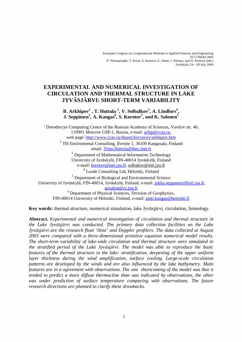
The numerical model used here is a three-dimensional ocean circulation model (Princeton Ocean Model) developed for coastal ocean applications by Blumberg and Mellor in 1987 [12] and adapted for the Lake Jyväsjärvi. Extensive tests with observed currents, water level fluctuations, and surface temperature distributions have been carried out during the development of the model for the Lake Jyväsjärvi. The present study is focused on short-term simulations of temperature and circulation patterns, on the description of forcing functions, simulation results and its comparison with observations for the Lake Jyväsjärvi. It makes a first step in developing a true climatology of the Lake Jyväsjärvi. Physical mechanisms responsible for observed short-term circulation patterns are considered more fully. The Princeton model was applied to the Lake Jyväsjärvi for a period in August 2003. The period was chosen for the model calibration because of an extensive set of subsurface current (Figure 1). During this period also conductivity temperature - depth (CTD) profile data collection was conducted in several profiles on the Lake Jyväsjärvi.

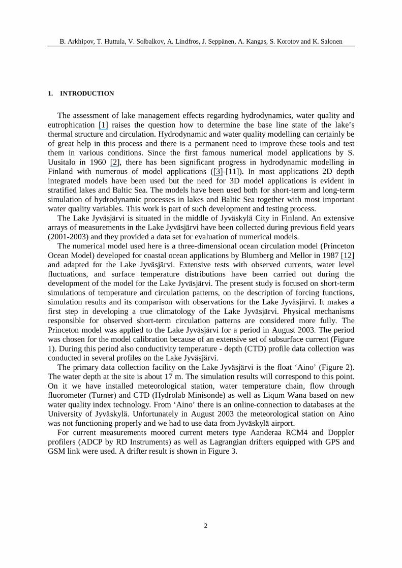
The primary data collection facility on the Lake Jyväsjärvi is the float ‘Aino’ (Figure 2). The water depth at the site is about 17 m. The simulation results will correspond to this point. On it we have installed meteorological station, water temperature chain, flow through fluorometer (Turner) and CTD (Hydrolab Minisonde) as well as Liqum Wana based on new water quality index technology. From ‘Aino’ there is an online-connection to databases at the University of Jyväskylä. Unfortunately in August 2003 the meteorological station on Aino was not functioning properly and we had to use data from Jyväskylä airport.

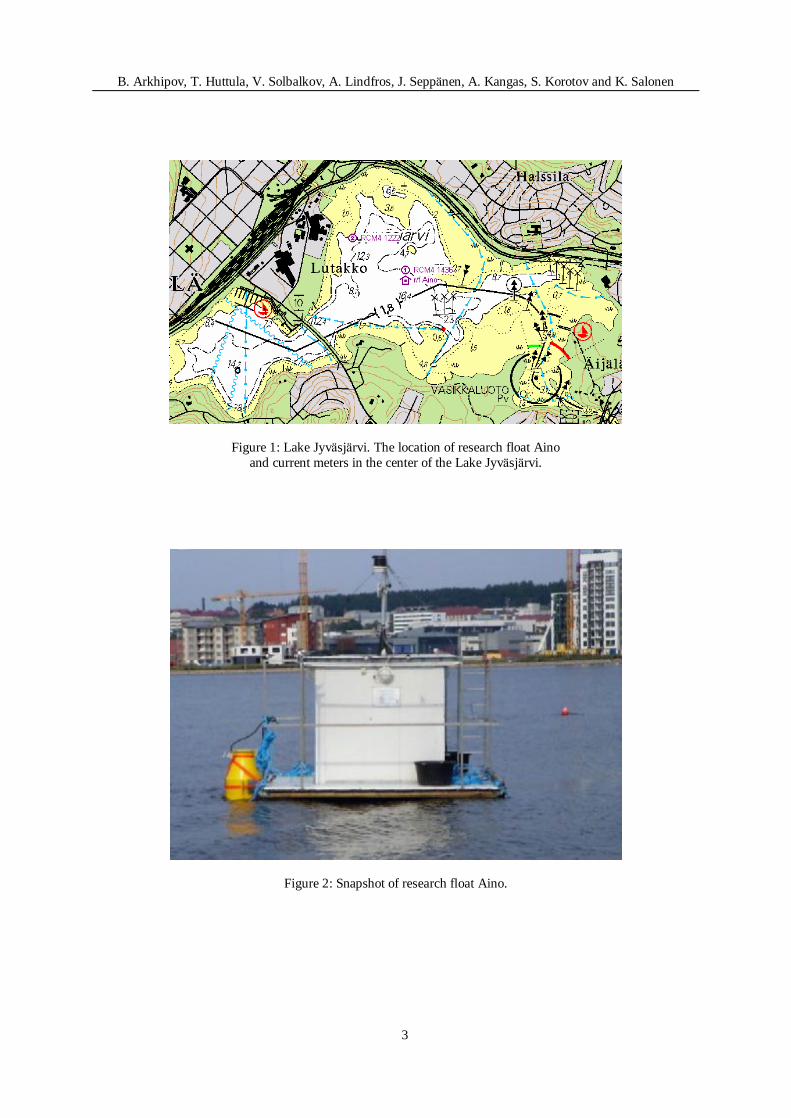
For current measurements moored current meters type Aanderaa RCM4 and Doppler profilers (ADCP by RD Instruments) as well as Lagrangian drifters equipped with GPS and GSM link were used. A drifter result is shown in Figure 3.

B. Arkhipov, T. Huttula, V. Solbalkov, A. Lindfros, J. Seppänen, A. Kangas, S. Korotov and K. Salonen

3

Figure 1: Lake Jyväsjärvi. The location of research float Aino and current meters in the center of the Lake Jyväsjärvi.

Figure 2: Snapshot of research float Aino.

B. Arkhipov, T. Huttula, V. Solbalkov, A. Lindfros, J. Seppänen, A. Kangas, S. Korotov and K. Salonen

4

Figure 3: Drifter track on 19.9.2002 10:12…15:38 on the Lake Jyväsjärvi. Below the buoy three cylinders 0,7-2,7 and 3-4 m (diameter 0,6 m and height 1 m). Wind was blowing from N with a velocity of 2-3 ms-1.

2. HYDRODYNAMIC MODEL

The Princeton model of Blumberg and Mellor [12] is a nonlinear, fully three-dimensional,

primitive equation, finite difference model that solves the heat, mass, and momentum conservation equations of fluid dynamics. The model is hydrostatic and Boussinesq so that density variations are neglected except where they are multiplied by gravity in the buoyancy force. The model uses time-dependent wind stress and heat flux forcing at the surface, zero heat flux at the bottom, free slip lateral boundary conditions, and quadratic bottom friction.

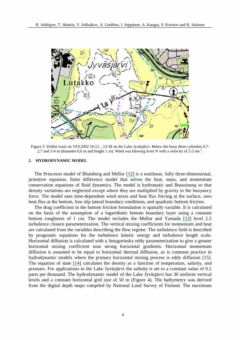
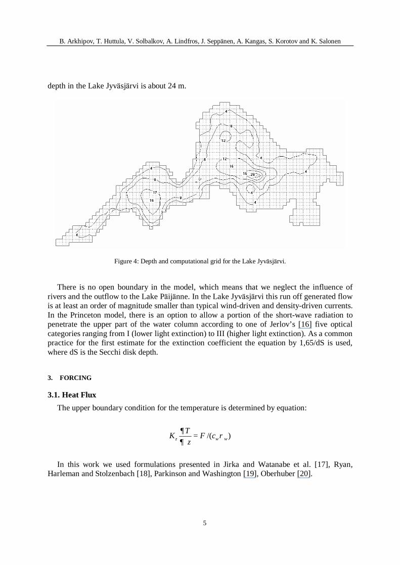
The drag coefficient in the bottom friction formulation is spatially variable. It is calculated on the basis of the assumption of a logarithmic bottom boundary layer using a constant bottom roughness of 1 cm. The model includes the Mellor and Yamada [13] level 2.5 turbulence closure parameterization. The vertical mixing coefficients for momentum and heat are calculated from the variables describing the flow regime. The turbulence field is described by prognostic equations for the turbulence kinetic energy and turbulence length scale. Horizontal diffusion is calculated with a Smagorinsky eddy parameterization to give a greater horizontal mixing coefficient near strong horizontal gradients. Horizontal momentum diffusion is assumed to be equal to horizontal thermal diffusion, as is common practice in hydrodynamic models where the primary horizontal mixing process is eddy diffusion [15]. The equation of state [14] calculates the density as a function of temperature, salinity, and pressure. For applications to the Lake Jyväsjärvi the salinity is set to a constant value of 0.2 parts per thousand. The hydrodynamic model of the Lake Jyväsjärvi has 30 uniform vertical levels and a constant horizontal grid size of 50 m (Figure 4). The bathymetry was derived from the digital depth maps compiled by National Land Survey of Finland. The maximum

B. Arkhipov, T. Huttula, V. Solbalkov, A. Lindfros, J. Seppänen, A. Kangas, S. Korotov and K. Salonen

5

depth in the Lake Jyväsjärvi is about 24 m.

Figure 4: Depth and computational grid for the Lake Jyväsjärvi.

There is no open boundary in the model, which means that we neglect the influence of

rivers and the outflow to the Lake Päijänne. In the Lake Jyväsjärvi this run off generated flow is at least an order of magnitude smaller than typical wind-driven and density-driven currents. In the Princeton model, there is an option to allow a portion of the short-wave radiation to penetrate the upper part of the water column according to one of Jerlov’s [16] five optical categories ranging from I (lower light extinction) to III (higher light extinction). As a common practice for the first estimate for the extinction coefficient the equation by 1,65/dS is used, where dS is the Secchi disk depth.

3. FORCING

3.1. Heat Flux The upper boundary condition for the temperature is determined by equation:

/( ) z w wTK F cz

∂ρ

∂=

In this work we used formulations presented in Jirka and Watanabe et al. [17], Ryan,

Harleman and Stolzenbach [18], Parkinson and Washington [19], Oberhuber [20].

B. Arkhipov, T. Huttula, V. Solbalkov, A. Lindfros, J. Seppänen, A. Kangas, S. Korotov and K. Salonen

6

Net heat flux ( )2F W m is the sum of snF short wave radiation, long radiation aF , back

radiation brF , latent lF and sensible flux SF :

sn a br l sF F F F F F= + − − − .

3.2. Momentum Flux The momentum flux from the surface is exhibited as wind stresses, determined by the

module and direction of wind:

22 x y

3, sin( ), cos( ), = 2a

dw

C Vρτ τ τ α τ τ α α π ϕρ= ⋅ = = − .

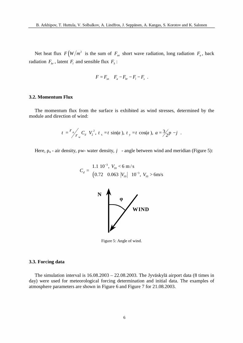
Here, ρa - air density, ρw- water density, ϕ - angle between wind and meridian (Figure 5):

( )3

10

310 10

1.1 10 , 6 m / s

0.72 0.063 10 , 6m/sd

VC

V V

−

−

⋅ <= + ⋅ ⋅ >

N φ

WIND

Figure 5: Angle of wind.

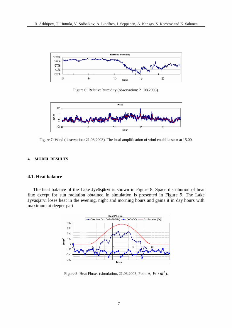
3.3. Forcing data The simulation interval is 16.08.2003 – 22.08.2003. The Jyväskylä airport data (8 times in

day) were used for meteorological forcing determination and initial data. The examples of atmosphere parameters are shown in Figure 6 and Figure 7 for 21.08.2003.

B. Arkhipov, T. Huttula, V. Solbalkov, A. Lindfros, J. Seppänen, A. Kangas, S. Korotov and K. Salonen

7

Figure 6: Relative humidity (observation: 21.08.2003).

Figure 7: Wind (observation: 21.08.2003). The local amplification of wind could be seen at 15.00.

4. MODEL RESULTS

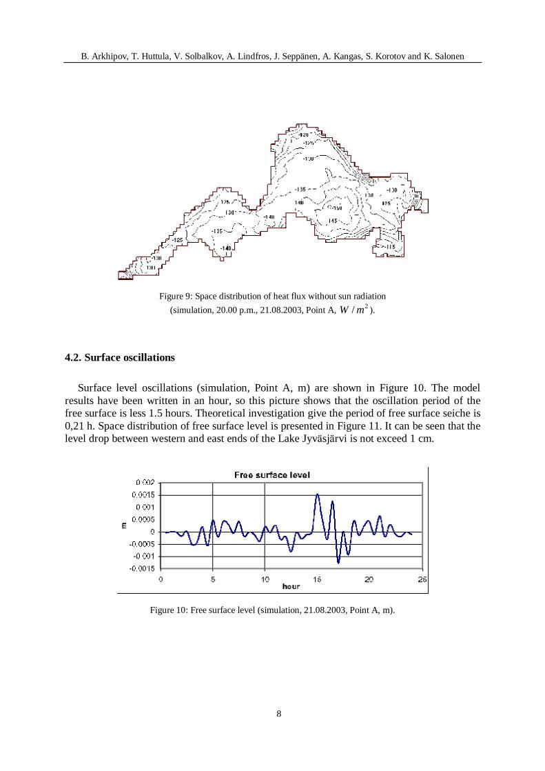
4.1. Heat balance The heat balance of the Lake Jyväsjärvi is shown in Figure 8. Space distribution of heat

flux except for sun radiation obtained in simulation is presented in Figure 9. The Lake Jyväsjärvi loses heat in the evening, night and morning hours and gains it in day hours with maximum at deeper part.

Figure 8: Heat Fluxes (simulation, 21.08.2003, Point A, 2/W m ).

B. Arkhipov, T. Huttula, V. Solbalkov, A. Lindfros, J. Seppänen, A. Kangas, S. Korotov and K. Salonen

8

Figure 9: Space distribution of heat flux without sun radiation (simulation, 20.00 p.m., 21.08.2003, Point A, 2/W m ).

4.2. Surface oscillations Surface level oscillations (simulation, Point A, m) are shown in Figure 10. The model

results have been written in an hour, so this picture shows that the oscillation period of the free surface is less 1.5 hours. Theoretical investigation give the period of free surface seiche is 0,21 h. Space distribution of free surface level is presented in Figure 11. It can be seen that the level drop between western and east ends of the Lake Jyväsjärvi is not exceed 1 cm.

Figure 10: Free surface level (simulation, 21.08.2003, Point A, m).

B. Arkhipov, T. Huttula, V. Solbalkov, A. Lindfros, J. Seppänen, A. Kangas, S. Korotov and K. Salonen

9

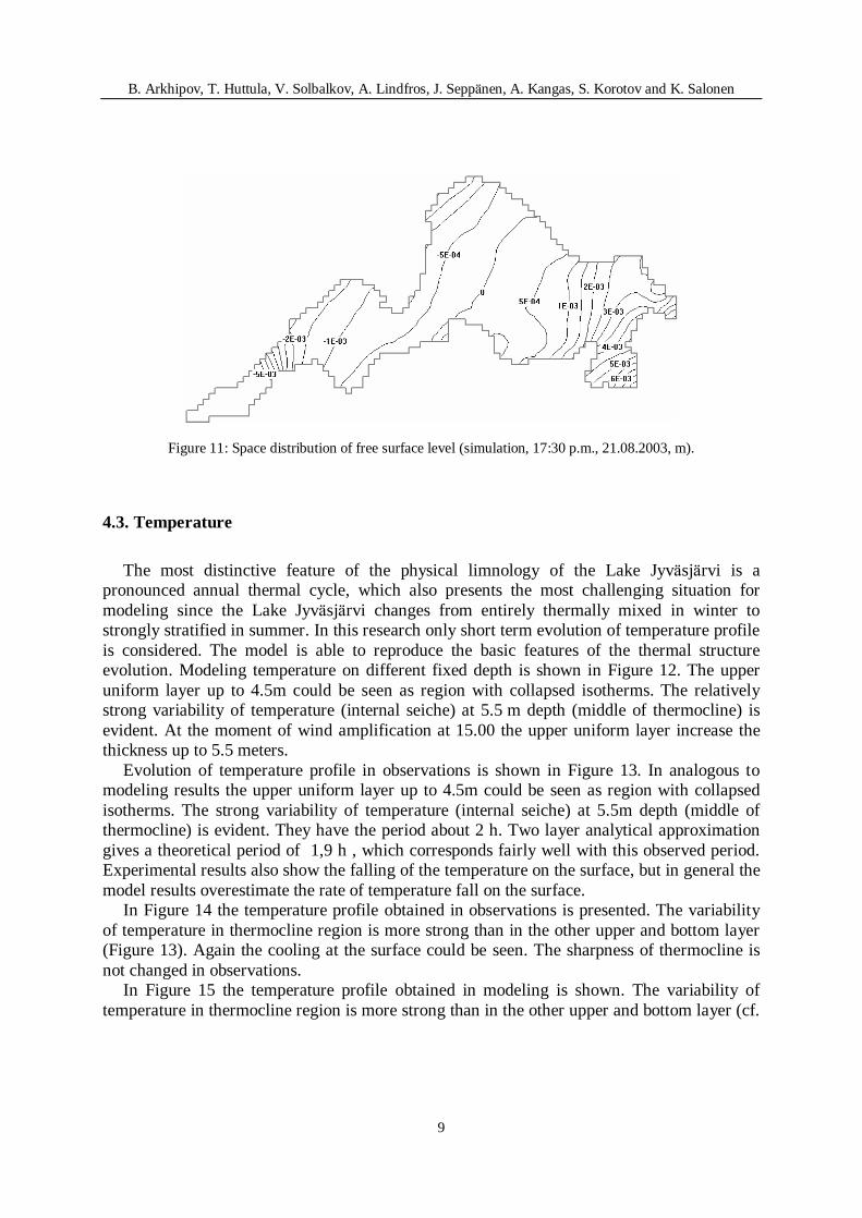
Figure 11: Space distribution of free surface level (simulation, 17:30 p.m., 21.08.2003, m).

4.3. Temperature The most distinctive feature of the physical limnology of the Lake Jyväsjärvi is a

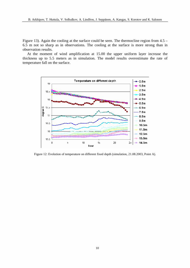
pronounced annual thermal cycle, which also presents the most challenging situation for modeling since the Lake Jyväsjärvi changes from entirely thermally mixed in winter to strongly stratified in summer. In this research only short term evolution of temperature profile is considered. The model is able to reproduce the basic features of the thermal structure evolution. Modeling temperature on different fixed depth is shown in Figure 12. The upper uniform layer up to 4.5m could be seen as region with collapsed isotherms. The relatively strong variability of temperature (internal seiche) at 5.5 m depth (middle of thermocline) is evident. At the moment of wind amplification at 15.00 the upper uniform layer increase the thickness up to 5.5 meters.

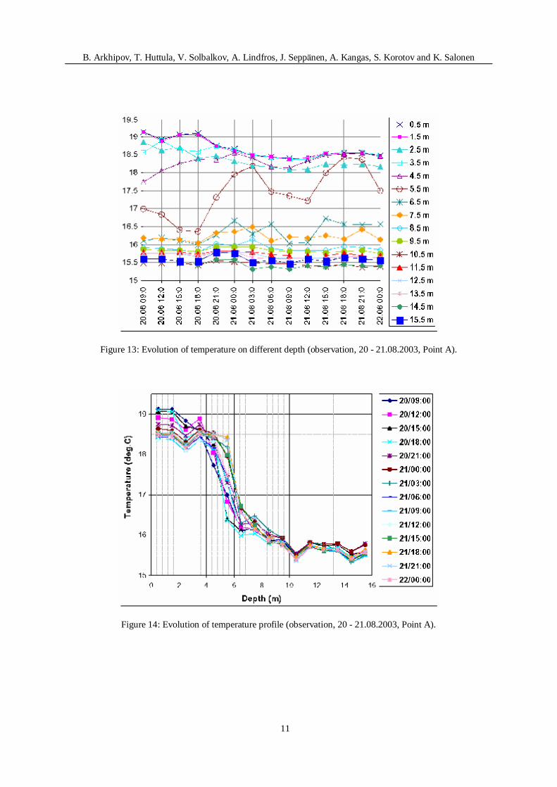
Evolution of temperature profile in observations is shown in Figure 13. In analogous to modeling results the upper uniform layer up to 4.5m could be seen as region with collapsed isotherms. The strong variability of temperature (internal seiche) at 5.5m depth (middle of thermocline) is evident. They have the period about 2 h. Two layer analytical approximation gives a theoretical period of 1,9 h , which corresponds fairly well with this observed period. Experimental results also show the falling of the temperature on the surface, but in general the model results overestimate the rate of temperature fall on the surface.

In Figure 14 the temperature profile obtained in observations is presented. The variability of temperature in thermocline region is more strong than in the other upper and bottom layer (Figure 13). Again the cooling at the surface could be seen. The sharpness of thermocline is not changed in observations.

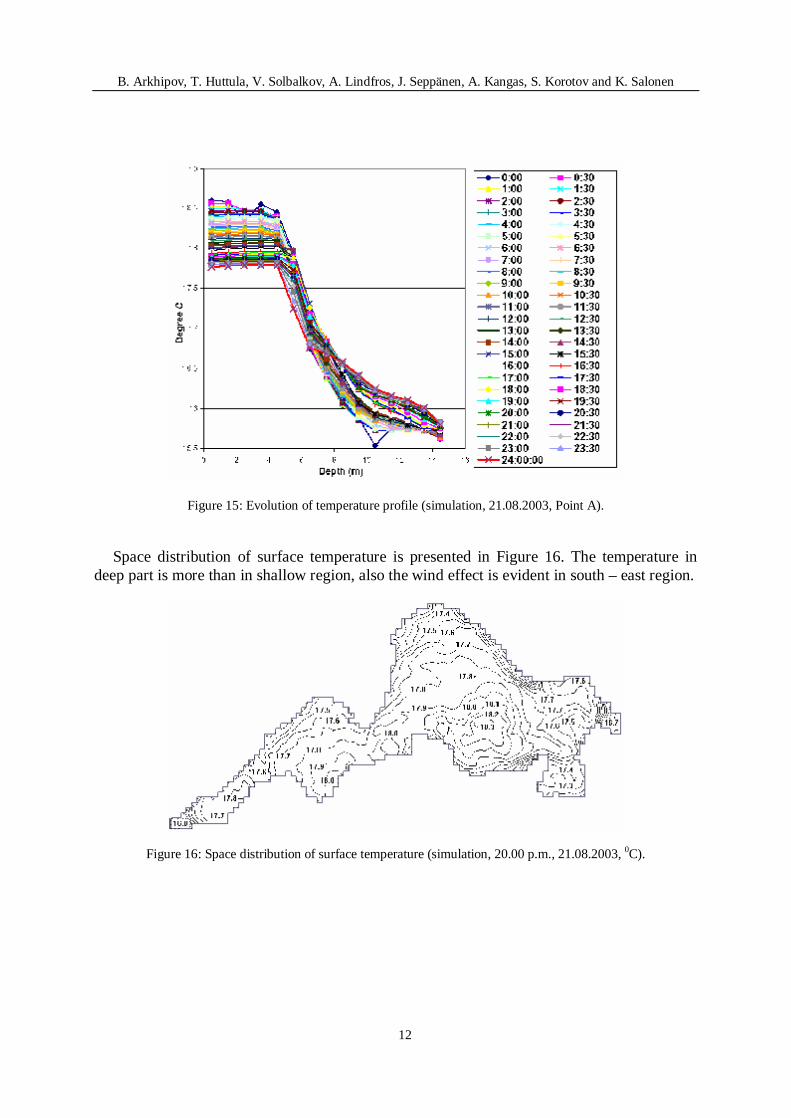
In Figure 15 the temperature profile obtained in modeling is shown. The variability of temperature in thermocline region is more strong than in the other upper and bottom layer (cf.

B. Arkhipov, T. Huttula, V. Solbalkov, A. Lindfros, J. Seppänen, A. Kangas, S. Korotov and K. Salonen

10

Figure 13). Again the cooling at the surface could be seen. The thermocline region from 4.5 – 6.5 m not so sharp as in observations. The cooling at the surface is more strong than in observation results.

At the moment of wind amplification at 15.00 the upper uniform layer increase the thickness up to 5.5 meters as in simulation. The model results overestimate the rate of temperature fall on the surface.

Figure 12: Evolution of temperature on different fixed depth (simulation, 21.08.2003, Point A).

B. Arkhipov, T. Huttula, V. Solbalkov, A. Lindfros, J. Seppänen, A. Kangas, S. Korotov and K. Salonen

11

Figure 13: Evolution of temperature on different depth (observation, 20 - 21.08.2003, Point A).

Figure 14: Evolution of temperature profile (observation, 20 - 21.08.2003, Point A).

B. Arkhipov, T. Huttula, V. Solbalkov, A. Lindfros, J. Seppänen, A. Kangas, S. Korotov and K. Salonen

12

Figure 15: Evolution of temperature profile (simulation, 21.08.2003, Point A).

Space distribution of surface temperature is presented in Figure 16. The temperature in

deep part is more than in shallow region, also the wind effect is evident in south – east region.

Figure 16: Space distribution of surface temperature (simulation, 20.00 p.m., 21.08.2003, 0C).

B. Arkhipov, T. Huttula, V. Solbalkov, A. Lindfros, J. Seppänen, A. Kangas, S. Korotov and K. Salonen

13

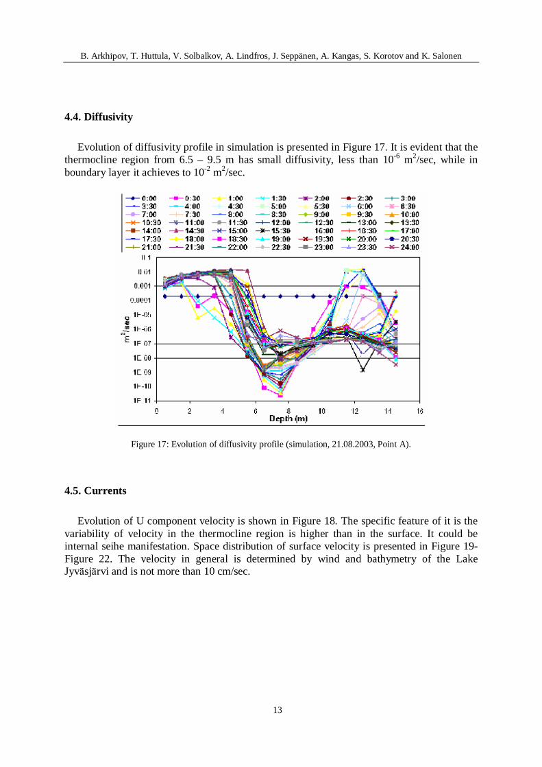
4.4. Diffusivity Evolution of diffusivity profile in simulation is presented in Figure 17. It is evident that the

thermocline region from 6.5 – 9.5 m has small diffusivity, less than 10-6 m2/sec, while in boundary layer it achieves to 10-2 m2/sec.

Figure 17: Evolution of diffusivity profile (simulation, 21.08.2003, Point A).

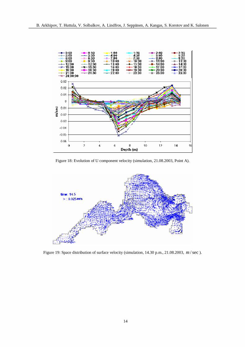
4.5. Currents Evolution of U component velocity is shown in Figure 18. The specific feature of it is the

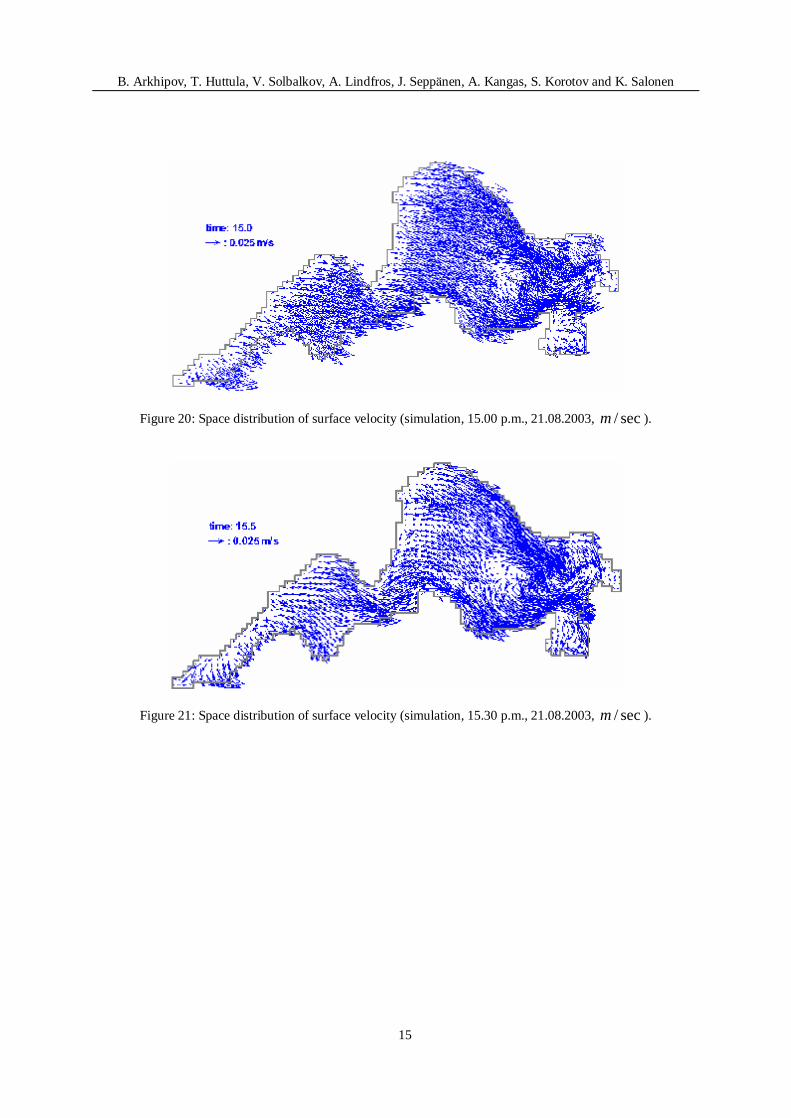
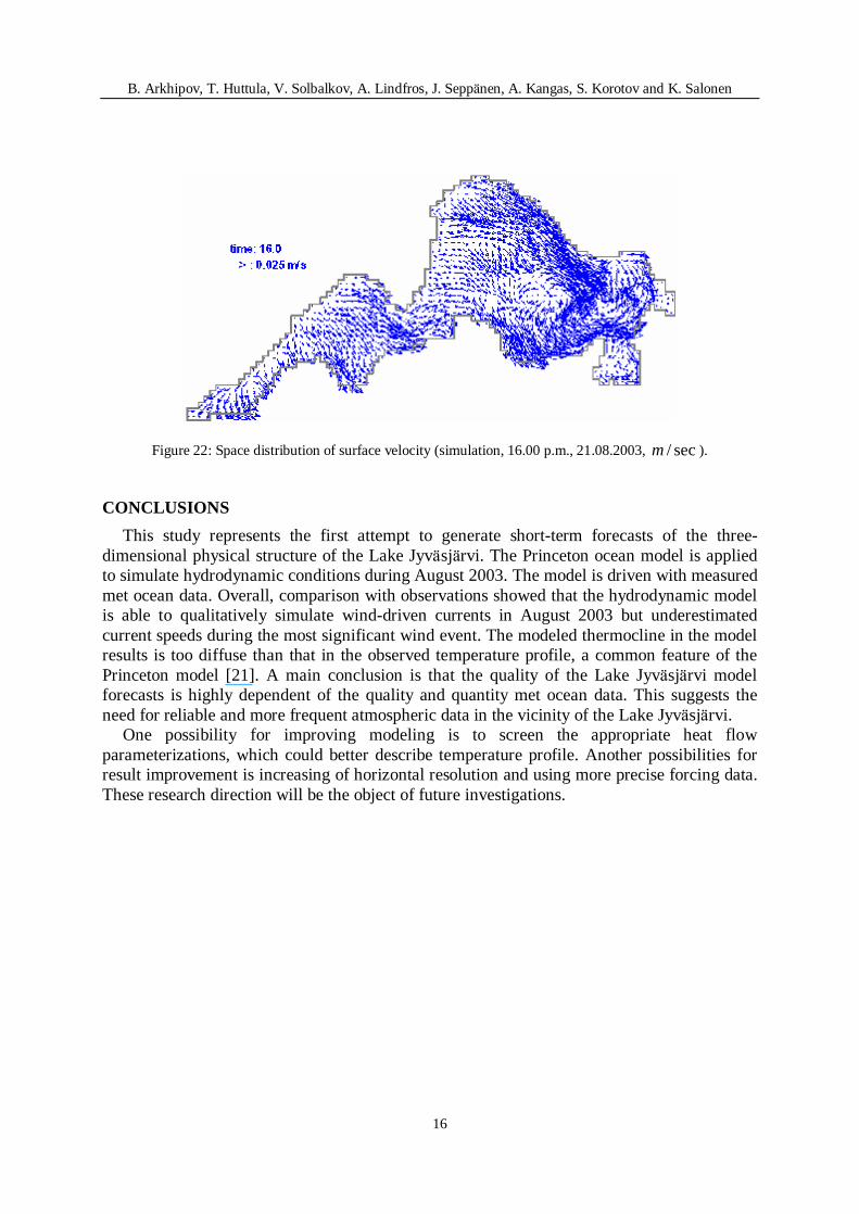
variability of velocity in the thermocline region is higher than in the surface. It could be internal seihe manifestation. Space distribution of surface velocity is presented in Figure 19-Figure 22. The velocity in general is determined by wind and bathymetry of the Lake Jyväsjärvi and is not more than 10 cm/sec.

B. Arkhipov, T. Huttula, V. Solbalkov, A. Lindfros, J. Seppänen, A. Kangas, S. Korotov and K. Salonen

14

Figure 18: Evolution of U component velocity (simulation, 21.08.2003, Point A).

Figure 19: Space distribution of surface velocity (simulation, 14.30 p.m., 21.08.2003, / secm ).

B. Arkhipov, T. Huttula, V. Solbalkov, A. Lindfros, J. Seppänen, A. Kangas, S. Korotov and K. Salonen

15

Figure 20: Space distribution of surface velocity (simulation, 15.00 p.m., 21.08.2003, / secm ).

Figure 21: Space distribution of surface velocity (simulation, 15.30 p.m., 21.08.2003, / secm ).

B. Arkhipov, T. Huttula, V. Solbalkov, A. Lindfros, J. Seppänen, A. Kangas, S. Korotov and K. Salonen

16

Figure 22: Space distribution of surface velocity (simulation, 16.00 p.m., 21.08.2003, / secm ).

CONCLUSIONS

This study represents the first attempt to generate short-term forecasts of the three-dimensional physical structure of the Lake Jyväsjärvi. The Princeton ocean model is applied to simulate hydrodynamic conditions during August 2003. The model is driven with measured met ocean data. Overall, comparison with observations showed that the hydrodynamic model is able to qualitatively simulate wind-driven currents in August 2003 but underestimated current speeds during the most significant wind event. The modeled thermocline in the model results is too diffuse than that in the observed temperature profile, a common feature of the Princeton model [21]. A main conclusion is that the quality of the Lake Jyväsjärvi model forecasts is highly dependent of the quality and quantity met ocean data. This suggests the need for reliable and more frequent atmospheric data in the vicinity of the Lake Jyväsjärvi.

One possibility for improving modeling is to screen the appropriate heat flow parameterizations, which could better describe temperature profile. Another possibilities for result improvement is increasing of horizontal resolution and using more precise forcing data. These research direction will be the object of future investigations.

B. Arkhipov, T. Huttula, V. Solbalkov, A. Lindfros, J. Seppänen, A. Kangas, S. Korotov and K. Salonen

17

REFERENCES [1] L.C. Bowling, K. Salonen. Heat uptake and resistance to mixing in small humic forest

lakes in southern Finland. Austr. J. Mar. Freshwater Res. 41: 747-759, 1990. [2] S. Uusitalo. The numerical calculation of wind effect on sea level elevations. Tellus 12,

427-435, 1960. [3] G. Schernewski, V. Podsetchine, H. Siegel and T. Huttula. Instruments for water quality

management and research in coastal zones: Flow and transport simulations across spatial scales. Periodicum biologorum, 102, Suppl. 1, 65-75, 2000a.

[4] G. Schernewski, V. Podsetchine, M. Asshoff, D. Garbe-Schönberg and T. Huttula. Spatial ecological structures in littoral zones and small lakes: Examples and future prospects of flow models as research tools. Arch. Hydrobiol.,Spec. Issues Advanc. Limnol. 55:227-241. Limnology and Lake Management, 2000b.

[5] J. Forsius, T. Huttula. Application of a mathematical model to a branched water course. Geophysica 19, 1:56-64, 1982.

[6] J. Koponen, E. Alasaarela, K. Lehtinen, J. Sarkkula, P. Simbierowitz, H. Vepsä and M. Virtanen. Modeling the dynamics of a large sea area. Publications of Water and Environment Research Institute No. 7. National Board of Waters and the Environment, Finland, 1992.

[7] J. Sarkkula, M. Virtanen. Modeling of water exchange in an estuary. Nordic Hydrology, 9, pp. 43-56, 1978.

[8] J. Sarkkula. Measuring and Modeling Flow and Water Quality in Finland. VITUKI Monographies No. 40, Waters Research Center VITUKI, Budapest, 1989.

[9] T. Huttula. (ed.), System analysis applications to water research in the Sovjet Union and Finland. Publications of Water and Environment Institute No. 3, National Board of Waters and Environment, Helsinki, 1989.

[10] V. Podsetchine, T. Huttula. Numerical simulation of wind-driven circulation in Lake Tanganyika. Aquatic Ecosystem Health and Management 3:55-64, 2000.

[11] H. Virta. 3D model of Lake Pääjärvi. MSc. thesis at the Department of Geophysics. University of Helsinki, 2001.

[12] A. Blumberg, G. Mellor. A description of the three-dimensional coastal ocean circulation model. In: Heaps, N. (Ed.), Three dimensional coastal ocean model. AGU, Washington, DC, 1987.

[13] G.L. Mellor, T. Yamada. Development of a turbulence closure model for geophysical fluid problems, Rev. Geophys., 20, 851–875, 1982.

[14] G.L. Mellor. An equation of state for numerical models of oceans and estuaries, J. Atmos. Oceanic Technol., 8, 609–611, 1991.

[15] A.F. Blumberg. Turbulent mixing processes in lakes, reservoirs and impoundments, in Physics-Based Modeling of Lakes, Reservoirs, and Impoundments, edited by W. G. Gray, pp. 79–104, Am. Soc. of Civ. Eng., New York, 1986.

[16] N.G. Jerlov. Marine Optics, 231 pp., Elsevier Sci., New York, 1976. [17] G.H. Jirka, M. Watanabe, K.H. Octavio, C.F. Cerco, D.R.F. Harleman. Mathematical

predictive models for cooling ponds and lakes. Part A: Model development and design

B. Arkhipov, T. Huttula, V. Solbalkov, A. Lindfros, J. Seppänen, A. Kangas, S. Korotov and K. Salonen

18

consideration. Ralph M. Parson Lab. for Water Res. and Hydrodinam. Rep. N 238, MIT, Cambridge, 199 p., 1978.

[18] P.J. Ryan, D.R.F. Harleman, K.D. Stolzenbach. Surface Heat Loss.Water Resources Research, 10(5), 930-938, 1974.

[19] C.L. Parkinson, W.M. Washington. A large scale numerical model of sea ice. J. Geophys. Res., 84, 311-337, 1979.

[20] J.M. Oberhuber. Simulation of the Atlantic Circulation with a coupled sea ice-mixed layer - isopycnal general circulation model. Max - Planck - Institut fuer meteorogie. Rep. N 59, 75 p., 1990.

[21] D. Beletsky, D.J. Schwab. Modeling circulation and thermal structure in Lake Michigan: Annual cycle and interannual variability Journal of Geophysical Research, VOL. 106, No. C9, 745–19,771, 2001.