experimental and analytical estimation of damping in beams ...

EXPERIMENTAL AND ANALYTICAL ESTIMATION OF DAMPING IN

BEAMS AND PLATES WITH DAMPING TREATMENTS

By

Wanbo Liu

Committee:

______________________________________

Dr Mark Ewing, Chairperson

_____________________________________

Dr Karan Surana

_____________________________________

Dr Richard Hale

_____________________________________

Dr Saeed Farokhi

_____________________________________

Dr Ronald Barrett-Gonzalez

Date defended

11-24-2008 i

Submitted to the graduate degree program in

Aerospace Engineering and the Graduate

Faculty of the University of Kansas School of

Engineering in Partial Fulfillment of the

Requirements for the Degree of

Doctor of Philosophy

ii

The Dissertation Committee for Wanbo Liu certifies

that this is the approved version of the following dissertation:



Committee:

______________________________________

Dr Mark Ewing, Chairperson

______________________________________

Dr Karan Surana

______________________________________

Dr Richard Hale

______________________________________

Dr Saeed Farokhi

______________________________________

Dr Ronald Barrett-Gonzalez

Date approved __________________________

iii



By

Wanbo Liu

November 2008

Abstract

The research presented in this dissertation is devoted to the problem of damping

estimation in engineering structures, especially beams and plates with passive damping

treatments. In structural design and/or optimization, knowledge about damping is essential.

However, due to the complexity of the dynamic interaction of system components, the

determination of damping, by either analysis or experiments, has never been straightforward.

In this research, currently-used methods are reviewed and gaps are identified first. Then both

analytical and experimental studies on the damping estimation are conducted and possibilities

of improvement are explored.

Various passive damping treatments using ViscoElastic Materials (VEMs) are designed,

manufactured and then added to aluminum and composite beams and plates. Experiments on

these damped structures are conducted. Currently used experimental methods, namely, the

free-decay method, the modal curve-fitting method and the Power Input Method (PIM), are

used to process the experimental data and investigate the damping characteristics. Especially,

1) experimental procedures of the power input method are carefully identified and

investigated; 2) the power input method is applied to non-uniformly damped structures; 3) the

iv

power input method is applied in an extended frequency range (from 0 to 5000 Hz) to meet

emerging needs of the transportation industries.

A new analytical power input method is proposed for evaluating the loss factor of built-

up structures, based on the finite element model with assigned properties of the constituents.

Finite Element (FE) models of beams and plates with various damping configurations are

developed so a frequency response solution suffices to provide mobility and energy results

needed by the new analytical power input method. The analytical power input method is

evaluated by comparison with the commonly used Modal Strain Energy (MSE) method.

Instead of making an approximate correction of the constant material properties, this

analytical power input method directly takes into account the frequency-dependent material

properties of the viscoelastic material using the MSC/NASTRAN direct frequency response

solution. Features of each method are compared and summarized. Especially, 1) the complex

frequency-dependency of viscoelastic materials used in constrained layer damping is modeled

using MSC Patran/NASTRAN; 2) a new procedure of estimating loss factors is presented,

using the concept of the power input method.

Particle damping is also investigated. A fluid analogy is proposed and applied to

composite beams and metallic plates. Results show that the fluid analogy can effectively

estimate peak damping frequencies and peak damping levels.

Both experimental and analytical loss factor results for various engineering structures are

presented and discussed.

v

Acknowledgements

The author would like first to express his gratitude to his advisor Dr Mark Ewing, whose

support and direction made the author’s PhD study possible.

The author also would like to thank his other dissertation committee members Dr Richard

Hale, Dr Saeed Farokhi, Dr Karan Surana and Dr Ronald Barrett-Gonzalez for their

assistance through the development of this dissertation.

The author seriously recognizes the teachings from other professors that have lectured

him at the University of Kansas.

The author appreciates all the help from the faculty and staff of the Department of

Aerospace Engineering as a whole for their support.

Special thanks go to the author’s parents Detian Liu and Ronglan Lu for their support and

understanding.

The author never forgets that he is indebted to many other people as well, though the

following can in no way include all the helpers on his study: Charles Gabel, Justin

Lohrmeyer, Patrick McNamee, Jim Weaver, Ashok Gandhi Pavanasam, Wannok Sio, and

Norman Holmskog.

vi

Table of Contents

Abstract......................................................................................................... iii

Acknowledgements ........................................................................................v

List of Figures ............................................................................................ viii

List of Tables .................................................................................................xi

Nomenclature .............................................................................................. xii

1. Introduction.............................................................................................1 1.1. Passive Damping ............................................................................................................. 1

1.1.1. Constrained Layer Damping.................................................................................. 1 1.1.2. Particle Damping ................................................................................................... 3

1.2. Loss Factor ...................................................................................................................... 3 1.2.1. Definition of Loss Factor....................................................................................... 4 1.2.2. Loss Factor and Damping Ratio ............................................................................ 4

1.3. Experimental Methods..................................................................................................... 5 1.3.1. Commonly-used Experimental Methods ............................................................... 5 1.3.2. Basic Principles of Experimental Power Input Method......................................... 7 1.3.3. Current Development of the Experimental Power Input Method........................ 10

1.4. Analytical Methods........................................................................................................ 15 1.4.1. Analytical Methods for Viscoelastic Damping.................................................... 15 1.4.2. Analytical Methods for Particle Damping ........................................................... 19

2. Structures with Viscoelastic Damping................................................21 2.1. Experimental Study ....................................................................................................... 21

2.1.1. Experimental Setup.............................................................................................. 21 2.1.2. Comparison of Experimental Responses with Analytical Responses.................. 23

2.2. Analytical Study ............................................................................................................ 25 2.2.1. Viscoelasticity...................................................................................................... 25 2.2.2. Finite Element Modeling of Viscoelastic Materials for Steady-State Analysis... 31 2.2.3. Finite Element Modeling of Sandwich Structures with Viscoelastic Core.......... 34 2.2.4. Validation of Finite Element Modeling ............................................................... 36 2.2.5. Comparison of Analytical Responses with Published Responses ....................... 39 2.2.6. Mathematical Model of Sandwich Plates with Viscoelastic Core: Theoretical

Approach Compared with Finite Element Method.............................................. 41 2.2.7. Analytical Power Input Method........................................................................... 50 2.2.8. Validation of Analytical Power Input Method..................................................... 51

2.3. Results and Discussion .................................................................................................. 52 2.3.1. Aluminum Plate with Partial Coverage Constrained Layer Damping................. 52 2.3.2. Aluminum Plate with Full Coverage Constrained Layer Damping..................... 60 2.3.3. Composite Honeycomb Sandwich Beam with Aluminum Stand-Off

Constrained Layer Damping................................................................................ 68 2.3.4. Composite Honeycomb Sandwich Beam with Plexiglas Stand-Off

Constrained Layer Damping................................................................................ 71

3. Structures with Particle Damping.......................................................76 3.1. Fluid Analogy................................................................................................................ 76

vii

3.1.1. Measurement of Particle Longitudinal Wave Speeds.......................................... 77 3.1.2. Measurement of Particle Internal Friction ........................................................... 79

3.2. Metallic Honeycomb Sandwich Plates with Different Particle Damping Treatments .. 80

4. Closure ...................................................................................................85 4.1. Summary........................................................................................................................ 85 4.2. Original Contributions to the Field of Structural Acoustics .......................................... 86 4.3. Conclusions ................................................................................................................... 86 4.4. Notes on Applying the Analytical Power Input Method ............................................... 89 4.5. Notes on Applying the Experimental Power Input Method .......................................... 89 4.6. Recommendations for Future Work .............................................................................. 90

Reference ......................................................................................................92

Appendices....................................................................................................98 A. Definition of Material Properties................................................................................... 98 B. Algorithm of Experimental Power Input Method in MATLAB.................................... 99 C. Algorithm of Analytical Power Input Method in MATLAB....................................... 100

viii

List of Figures

Figure 1.1 Schematic of constrained layer damping treatment. (a) Undeformed structure; (b)

deformed structure. ....................................................................................................... 2 Figure 1.2 Schematic of stand-off constrained layer damping treatment. (a) Undeformed

structure; (b) deformed structure................................................................................... 2 Figure 1.3 Schematic of particle damping treatment. .............................................................. 3 Figure 1.4 Relationship between loss factor η and damping ratio ζ. ...................................... 4

Figure 1.5 Measured free-decay time history of a sandwich honeycomb composite panel at

973 Hz showing multi-modal interferenece. ................................................................. 6 Figure 1.6 The mode shape of Wu, Agren and Sundback’s (1997) [89] 0.545×0.460×0.005 m

steel plate at 2473 Hz. ................................................................................................. 12 Figure 1.7 Bloss and Rao’s (2005) [9] comparison of the decay method and the power input

method. (a) Loss factors of the undamped plate; (b) loss factors of the damped plate.

..................................................................................................................................... 14 Figure 2.1 Experimental instruments. (a) A shaker attached to the test article through a force

transducer and an aluminum connector; (b) Polytec OFV 056 laser scanning head... 22 Figure 2.2 A typical experimental setup in this research. ..................................................... 22 Figure 2.3 Aluminum plate with full coverage constrained layer damping. (a) The plate as a

test article with scanning points defined; (b) the plate as a finite element model with

the driving point illustrated. ........................................................................................ 23 Figure 2.4 Comparison of the measured and predicted responses of a damped aluminum

plate. (a) Measured mobility at 239 Hz; (b) measured mobility at 3516 Hz; (c)

computed mobility at 239 Hz; (d) computed mobility at 3519 Hz. ............................ 24 Figure 2.5 Models of viscoelastic materials. (a) Maxwell model; (b) Kelvin-Voigt model; (c)

standard linear solid model. ........................................................................................ 27 Figure 2.6 Generalized models of viscoelastic materials. (a) Generalized Kelvin model; (b)

Generalized Maxwell model. ...................................................................................... 28 Figure 2.7 Material properties of 3M F9469PC at 20 °C used in this research extracted from

manufacturer’s nomograph. ........................................................................................ 34 Figure 2.8 Finite element models of a sandwich structure with viscoelastic core (facesheets

are in blue and viscoelastic core is in grey). (a) Plate elements with offsets of half of

the plate thickness, attached to solid elements; (b) plate elements with translational

degrees-of-freedom connected to solid elements by rigid links; (c) solid elements for

all three layers. ............................................................................................................ 35 Figure 2.9 Real and approximate linear representations of bending deflections. (a) Real

representation; (b) linear representation...................................................................... 36 Figure 2.10 Convergence study of a partially-covered sandwich plate. (a) Natural

frequencies; (b) strain energy ratios. ........................................................................... 37 Figure 2.11 Through-thickness discretization study using the modal strain energy method

(model 1: one solid element for each layer; model 2: two solid elements for each

layer; model 3: four solid elements for each layer)..................................................... 38 Figure 2.12 Displacement of the viscoelastic layer in relation to the displacement of the base

layer and the constraining layer. ................................................................................. 39

ix

Figure 2.13 Comparison of mechanical impedance results of Lu and Everstine’s (1980) [52]

beam. (a) Lu and Everstine’s result (Solid line: experimental results; Dots: Nastran

results); (b) Present result of this research. ................................................................. 40 Figure 2.14 Geometry of the sandwich plate with viscoelastic core. (a) Sign convention; (b)

thicknesses of the 3 layers........................................................................................... 41 Figure 2.15 Finite element model of the steel sandwich plate with viscoelastic core. .......... 49 Figure 2.16 Comparison of theoratical results and finite element results of the steel sandwich

plate with viscoelastic core. ........................................................................................ 50 Figure 2.17 Validation of the analytical power input method. (a) The finite element model of

the plate with the driving point defined; (b) The calculated loss factor of the plate. .. 52 Figure 2.18 Plate with partial coverage constrained layer damping. (a) The plate as a test

article with scanning points defined; (b) the plate as a finite element model with the

excitation point illustrated........................................................................................... 53 Figure 2.19 Loss factors of the aluminum plate with partial coverage constrained layer

damping by experimental power input method, free decay method and modal curve-

fitting method. ............................................................................................................. 54 Figure 2.20 Loss factor results of the aluminum plate with partial coverage constrained layer

damping in 2400-2600 Hz obtained using different stinger lengths. .......................... 55 Figure 2.21 Loss factors of the aluminum plate with partial coverage constrained layer

damping by analytical power input method and modal strain energy method............ 57 Figure 2.22 Selected mode shapes of the plate with partial coverage constrained layer

damping. (a) Mode shape at 2118 Hz; (b) mode shape at 2913 Hz. ........................... 58 Figure 2.23 Comparison of loss factors of the plate with partial coverage constrained layer

damping by the analytical power input method and the modal strain energy method

with the experimental free decay method and the modal curve-fitting method. ......... 59 Figure 2.24 Loss factors of the plate with partial coverage constrained layer damping by the

experimental power input method and analytical power input method. ..................... 59 Figure 2.25 Plate with full coverage constrained layer damping. (a) The plate as a test article

with scanning points defined; (b) the plate as a finite element model with the

excitation point illustrated........................................................................................... 61 Figure 2.26 Loss factors of the plate with full coverage constrained layer damping by the

experimental power input method and free decay method.......................................... 61 Figure 2.27 Loss factors of the plate with full coverage constrained layer damping by the

analytical power input method, modal strain energy method and free decay method. 62 Figure 2.28 Loss factors of the plate with full coverage constrained layer damping by the

experimental power input method and analytical power input method. ..................... 63 Figure 2.29 Low Loss factors of the plate with full coverage constrained layer damping

driven at an anti-node line by the experimental power input method and analytical

power input method..................................................................................................... 65 Figure 2.30 The mode shape of the plate with full coverage constrained layer damping at 157

Hz and the deflection shape in the vicinity of this mode. (a) The mode shape at 157

Hz; (b) deflection shape at 149 Hz.............................................................................. 65 Figure 2.31 The mode shape of the plate with full coverage constrained layer damping at 475


Hz; (b) deflection shape at 443 Hz.............................................................................. 66 Figure 2.32 High loss factors of the plate with full coverage constrained layer damping

driven at a node line by the experimental power input method and analytical power

input method................................................................................................................ 67

x

Figure 2.33 The mode shape of the plate with full coverage constrained layer damping at 475


Hz; (b) deflection shape at 443 Hz.............................................................................. 67 Figure 2.34 The mode shape of the plate with full coverage constrained layer damping at 475


Hz; (b) deflection shape at 639 Hz.............................................................................. 67 Figure 2.35 Composite honeycomb sandwich beam with aluminum stand-off constrained

layer damping treatment. (a) The beam as a test article; (b) the beam as a finite

element model. ............................................................................................................ 69 Figure 2.36 Loss factors of the composite honeycomb sandwich beam with aluminum stand-

off constrained layer damping treatment by the experimental power input method and

analytical power input method. ................................................................................... 71 Figure 2.37 Composite honeycomb sandwich beam with Plexiglas stand-off constrained

layer damping treatment. (a) The beam as a test article; (b) the beam as a finite

element model. ............................................................................................................ 72 Figure 2.38 Loss factors of the composite honeycomb sandwich beam with Plexiglas stand-

off constrained layer damping by the experimental power input method and the

analytical power input method. ................................................................................... 73 Figure 2.39 Summary of viscoelastic damping examples. (a) Mean loss factor from 0 to 3000

Hz; (b) ratio of mean loss factor to overall treatment mass. ....................................... 75 Figure 3.1 Particle displacement mode shape by a fluid resonance analogy in a cavity. (a)

Two ends open; (b) two ends closed. .......................................................................... 76 Figure 3.2 Experimental setup for longitudinal wave speed measurements of particles. ...... 77 Figure 3.3 Root mean square plot of mobility functions at cross sections of tubes with

different Inner Diameters (ID). ................................................................................... 78 Figure 3.4 Measured mobility resonances of the glass microbubbles in the 2 cm inner

diameter tube. (a) K1 microbubbles; (b) K30 microbubbles; (c) K37 microbubbles. 78 Figure 3.5 Angle of repose test of different glass microbubbles. (a) K1; (b) K20; (c) K37. . 79 Figure 3.6 Schematic of flowability test instrument. ............................................................. 80 Figure 3.7 Sandwich honeycomb plates with particle damping. (a): Schematic of damped

plates; (b): the three specimens filled with different particles. ................................... 81 Figure 3.8 Comparison of loss factors of metallic sandwich honeycomb plates with K1, K20

and K37 particles by the experimental power input method and the modal curve-

fitting method. ............................................................................................................. 83 Figure 3.9 Summary of particle damping examples. (a) Max loss factor; (b) ratio of mean

loss factor to treatment mass. ...................................................................................... 84

xi

List of Tables

Table 2.1 Description of the plate with full coverage constrained layer damping................. 23 Table 2.2 Characteristics of viscoelastic material properties................................................. 33 Table 2.3 Convergence study of in-plane discretization........................................................ 37 Table 2.4 Configuration of Lu and Everstine’s (1980) [52]beam.......................................... 39 Table 2.5 Description of the steel sandwich plate with viscoelastic core for theoretical and

finite element method comparison .............................................................................. 49 Table 2.6 Description of the plate with partial coverage constrained layer damping............ 53 Table 2.7 Description of the plate with full coverage constrained layer damping treatment. 61 Table 2.8 Description of the plate with aluminum stand-off constrained layer damping...... 69 Table 2.9 Description of the beam with Plexiglas stand-off constrained layer damping....... 72 Table 2.10 Summary of viscoelastic damping examples ....................................................... 74 Table 3.1 Internal friction tests of K1, K20 and K37 glass microbubbles............................. 80 Table 3.2 Description of metallic sandwich honeycomb plates............................................. 82 Table 3.3 Description of K1, K20 and K37 glass microbubbles ........................................... 82 Table 3.4 Summary of particle damping examples................................................................ 84

xii

Nomenclature

c = wave speed of glass microspheres

( )r

SE = system’s overall average strain energy from all components of the natural

mode r for the modal strain energy method ( )r

SiE = average strain energy in material i when the structure deforms at the natural

mode r for the modal strain energy method

DE = energy dissipated per cycle during period T

KE = average kinetic energy

SE = average strain energy

TotE = total mechanical (stored/vibrational) energy

E = elastic modulus

*E = complex elastic modulus

'E = real part of elastic modulus

"E = imaginary part of elastic modulus

( )tFf

= force at the driving point

( )ωf

F = Fourier transform of ( )tFf

f = frequency

rf = rth modal frequency calculated with the core shear modulus as 2,REFG for the

modal strain energy method

iG = shear modulus of the elastic layers i in sandwich structures

( )2G f′ = real part of the shear modulus of the viscoelastic layer 2

( )2G f′′ = imaginary part of the shear modulus of the viscoelastic layer 2

2,REFG = real part of the shear modulus of the viscoelastic layer 2 used in normal

modes calculation for the modal strain energy method

REFg = reference element damping coefficient used in normal modes calculation for

the modal strain energy method

g = overall structural damping coefficient

KE = max kinetic energy of the sandwich plate

im = mass of portion i for the experimental power input method

PE = max potential energy of the sandwich plate

DP = dissipated power, ( ) ( )1/ / 2D D DP T E Eω π= =

IP = input power

( )0f fF VR = cross correlation between the driving point force and driving point velocity

( )0i iV VR = auto-correlation of the velocity at point i

( )f fF F

S ω = power spectrum density of the driving point force

( )f fF V

S ω = cross power spectrum density between the driving point force and driving

point velocity

xiii

( )i i

V VS ω = power spectrum density of the velocity at points i

SE = max strain energy of the sandwich plate

T = period of a vibrational cycle

( )TR f = tabular function representing the real part of the complex moduli

( )TI f = tabular function representing the imaginary part of the complex moduli

it = thickness of layer i for the sandwich plate

iu = in plane displacement variable in x direction for layer i of the sandwich plate

V = velocity

( )fV t = velocity at the driving point

iv = in plane displacement variable in y direction for layer i of the sandwich plate

v = viscosity coefficient w = transverse displacement variable in z direction of the sandwich plate

( )ffY ω = mobility (velocity/force) of the driving point

( )ifY ω = mobility (velocity/force) between the driving point f and the point i

( )Z ω = impedance (force/velocity)

σ = stress

ε = strain

η = system loss factor

iη = material loss factor for material i

VEMη = material loss factor for the viscoelastic material

( )rη = system’s modal loss factor at the rth mode of the modal strain energy method

( ) 'rη = system’s adjusted modal loss factor for the rth mode of the modal strain

energy method

µ = Poisson’s ratio

ρ = density

ω = angular frequency

1ω = lower limit of the frequency band

2ω = upper limit of the frequency band

Cω = center frequency of the frequency band [ ]

21,ωω

ω∆ = bandwidth

P , Q = differential operators for stress and strain

P , Q = polynomials of the Laplace variable s for stress and strain

[ ]M = mass matrix

[ ]B = damping matrix

[ ]K = stiffness matrix

= time average

1

1. Introduction

Most engineering structures experience vibrational motion. Unwanted vibrations can

result in premature structural fatigue and/or failure, and often unpleasant noise. Damping

characteristics represent the structure’s ability to dissipate vibrational energy, and thus

represent the structure’s ability to suppress unwanted vibration. Estimation of damping in

engineering structures has been a developing science in both analytical and experimental

respects.

Generally speaking, the methods to increase damping can be categorized into two

categories: passive damping and active damping. Full-scale implementation of active and

semi-active damping treatment has been slow due to high costs and complexity. Passive

damping as a well-developed technique, in general, is more simple and cost-effective [69].

1.1. Passive Damping

Among passive damping treatments, Constrained Layer Damping (CLD) and Particle

Damping (PD) are the two most commonly-used methods.

1.1.1. Constrained Layer Damping

In constrained layer damping, a thin damping layer (usually viscoelastic materials) is

added to the structure, and then covered by a constraining layer, as shown in Figure 1.1.

When the base structure deforms, the damping layer is loaded in shear. Thus, under dynamic

load, the viscoelastic material dissipates energy by disrupting the bonds of its long-chain

molecules to convert kinetic energy to thermal energy (heat). An optional segmented spacer

can be added in between the base structure and the damping layer to amplify the deformation

of the base structure, often for structures with high specific stiffness, e.g., honeycomb

2

sandwich composites. In this case, the damping treatment is called Stand-Off Constrained

Layer Damping (SOCLD). Composite honeycomb sandwich structures do not deform much

under external excitation due to their high stiffness. Thus, if constrained layer damping is

applied directly on to the surface of such structures, there will be a lack of shear strain energy

in the viscoelastic layer. To solve this problem, stand-offs can be added to amplify the

deformation. These stand-offs should have high shear stiffness but near-zero bending

stiffness.

(a)

(b)

Figure 1.1 Schematic of constrained layer damping treatment. (a) Undeformed structure; (b) deformed

structure.

(a)

(b)

Figure 1.2 Schematic of stand-off constrained layer damping treatment. (a) Undeformed structure; (b)

deformed structure.

Constraining layer

Damping layer

Base structure

Low shear in damping layer

High shear in damping layer

Constraining layer

Damping layer

Base structure

Stand-off

Surface deformation amplified

3

1.1.2. Particle Damping

In particle damping, the damper is an enclosure or enclosures filled with particles made

of a variety of materials (e.g., lead, steel, tungsten, glass, etc.), as shown in Figure 1.3. The

energy loss is due to the inter-particle and particle-wall friction and inelastic impact. Unlike

constrained layer damping, particle damping can be used over a broad range of temperature

due to the intrinsic insensitivity to temperature of its damping materials. On the other hand,

the effect of any moisture in the medium may need to be considered if the temperature is

below the freezing point or if the particles are easily stuck together due to moisture. The

mechanism of particle damping is still not fully understood. It has been found to be closely

related to many factors, including particle size, particle density, particle shape, particle

surface friction, vibrational direction, packing ratio, vibration amplitude, etc. Once the region

to install particles is determined, the only design variables left are the particle type, the cavity

depth and the packing ratio.

Figure 1.3 Schematic of particle damping treatment.

1.2. Loss Factor

The damping loss factor is widely accepted as one of the major damping indices, and it is

used throughout this research. Hence, it is introduced first.

Particles

4

1.2.1. Definition of Loss Factor

The loss factor of a system is defined in energy terms [71] [8] [39] [24]:

2

D D

Tot Tot

P E

E Eη

ω π= = (1.1)

where DP is the dissipated power; Tot

E is the total mechanical (stored) energy, which is the

summation of average strain energy and average kinetic energy, Tot S KE E E= + ; DE is the

energy dissipated per cycle during period T, 1

2D D DP E E

T

ωπ

= = ; ω is the angular frequency.

1.2.2. Loss Factor and Damping Ratio

Figure 1.4 Relationship between loss factor η and damping ratio ζ.

In many references (Reference [35], Reference [59] and Section 7 in reference [78]), it is

stated that 1 2Qη ζ= = , where ζ is the damping ratio and Q is the quality factor. This is

usually accepted as the relationship between loss factor and damping ratio. However, the

accuracy is conditional. As pointed out by Nashif, Jones and Henderson (1985) [59] and

Graessner and Wong (1992) [36], 1 2 1 1Q ζ η η− = = + − − , so the loss factor is actually

Loss facto

r, η

(unitle

ss)

1.0

0.8

0.6

0.4

0.2

0

η =2ζ

η =2ζ 21 ζ−

0 0.1 0.2 0.3 0.4 0.5

Damping ratio, ζ (unitless)

5

22 1η ζ ζ= − . Thus, 2η ζ= is accurate within 5% for 3.00 ≤≤η . The comparison is

plotted in Figure 1.4.

1.3. Experimental Methods

1.3.1. Commonly-used Experimental Methods

Currently-used experimental methods of damping estimation can be broadly classified

into three groups [15] [17] [66], as briefly summarized below.

1) Time-domain free-decay methods. The method is based on the observation of the

time history of energy dissipation. In particular the response decay is expected to be

exponential when a single mode is excited. In the high frequency ranges, where

modal density is high, the time history curve usually shows beating, as shown in

Figure 1.5. This causes difficulty fitting a straight line to the log of the decay-rate

curve. Loss factors have been shown to vary with measurement points [71]. Also,

irregularities in decay history may occur if the excitation frequency does not quite

coincide with the natural frequency Section 4.4.2.2 in reference [24]. The free decay

method is best suited for lightly damped structures (if a directly-attached excitation is

used) in the low and middle frequency range.

2) Frequency-domain modal curve-fitting methods. These methods determine loss

factors at each individual natural mode, using frequency response function (FRF)

data measured from steady-state response. Modal frequencies are identified at the

peak resonance frequencies and modal damping is identified by the "width" of the

resonance peak. As an alternative, some techniques attempt to match measured data

6

with an analytical expression, often called curve-fitting. Difficulty in mode

identification arises as modal coupling and damping increases.

3) Power input method. The concept is directly based on the definition of structural

energy losses. Thus, there is no theoretical limitation on broad frequency application.

The concept of using the power input method to measure structural loss appeared in

the late 1970’s. However, due to the limitation on measurement instrumentation and

computational capabilities, development has been slow. It is not mentioned in the

general surveys in Cremer, Heckl and Ungar (1973) [22], Chu and Wang (1980) [19]

and Soovere and Drake (1985) [78], but it gradually draws more attention as shown

in literature [39], [66], [16], [17] and [18]. Recently the power input method appears

as an alternative method in the general survey by Cremer, Heckl and Petersson

(2005) [24]. The power input method is proven to have advantages over the other two

methods, though understanding of the experimental procedure is still developing.

Therefore, this method is given special attention in the current research.

Figure 1.5 Measured free-decay time history of a sandwich honeycomb composite panel at 973

Hz showing multi-modal interferenece.

Time, t (second)

1.825 1.85 1.875 1.9

Velo

city, V (m

m/s

econd) 2.5

0

2.5

7

1.3.2. Basic Principles of Experimental Power Input Method

The concept of the power input method to measure the loss factor is based directly on the

equation that defines this quantity, as shown in Equation (1.1) which is restated as:

2

D D

Tot Tot

P E

E Eη

ω π= = (1.1)

In a practical measurement, the following two steps are usually taken first.

1) As for the numerator, the input power is eventually converted into heat, which cannot

be easily measured. However, for a steady-state vibration, the dissipated power of the

system DP equals the input power IP from the excitation. Thus, if the structure is

driven at a single point, the input power can be estimated from the time-averaged

product of the force at the driving point ( )fF t and the velocity at the driving point

( )tVf

: ( ) ( )D I f fP P F t V t= = ⋅ .

2) As for the denominator, the total mechanical energy Tot

E cannot be easily measured

either, because it consists of two parts: the average kinetic energy and the average

strain energy, where average strain energy is hard to measure directly. So it is

replaced with twice the average kinetic energy KE [9][37][39][40], that is

2Tot KE E= ( )2

v

V t dvρ= ∫ .

Now the loss factor in time-averaged terms is [39]:

( ) ( )( )2

f f

v

F t V t

V t dvη

ω ρ

⋅=

∫ (1.2)

Specifically, the input power is:

( ) ( ) ( ) ( ) ( ) ( )0 0

0 Re Ref f f f f ff f F V F V ff F FF t V t R S d Y S dω ω ω ω ω

∞ ∞

⋅ = = = ∫ ∫ (1.3)

8

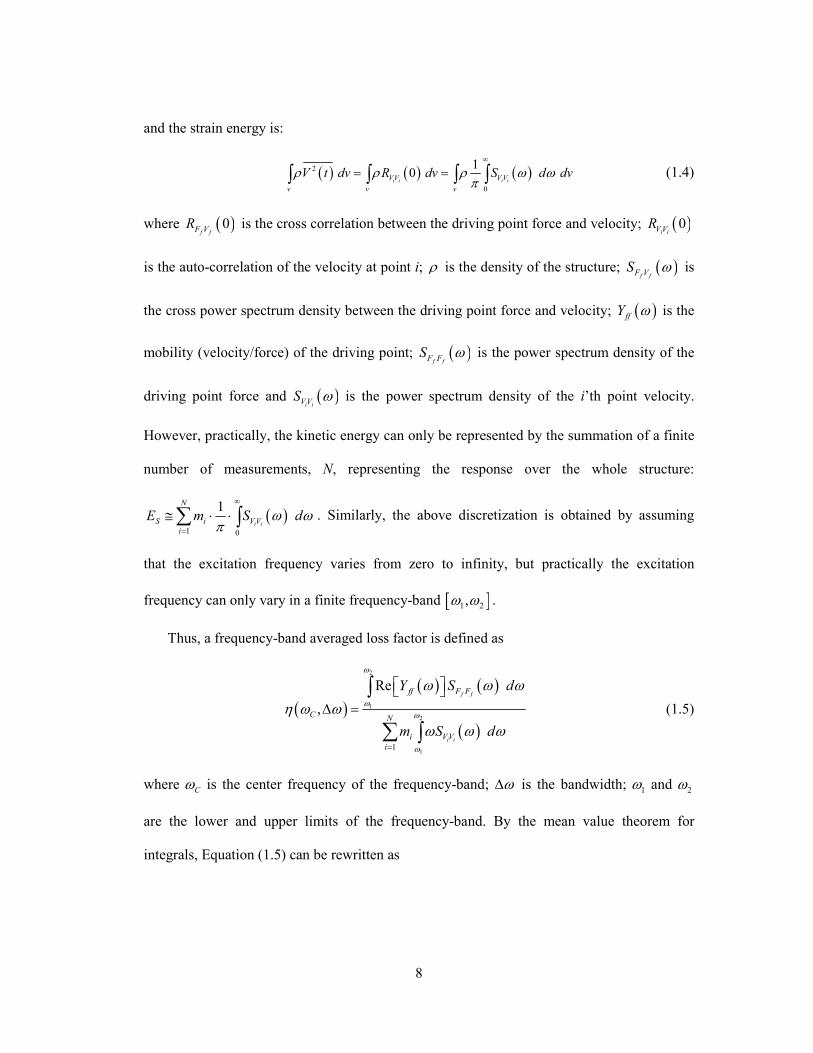
and the strain energy is:

( ) ( ) ( )2

0

10

i i i iVV V V

v v v

V t dv R dv S d dvρ ρ ρ ω ωπ

∞

= =∫ ∫ ∫ ∫ (1.4)

where ( )0f fF VR is the cross correlation between the driving point force and velocity; ( )0

i iV VR

is the auto-correlation of the velocity at point i; ρ is the density of the structure; ( )f fF VS ω is

the cross power spectrum density between the driving point force and velocity; ( )ffY ω is the

mobility (velocity/force) of the driving point; ( )f fF FS ω is the power spectrum density of the

driving point force and ( )i iV VS ω is the power spectrum density of the i’th point velocity.

However, practically, the kinetic energy can only be represented by the summation of a finite

number of measurements, N, representing the response over the whole structure:

( )1 0

1i i

N

S i V V

i

E m S dω ωπ

∞

=

≅ ⋅ ⋅∑ ∫ . Similarly, the above discretization is obtained by assuming

that the excitation frequency varies from zero to infinity, but practically the excitation

frequency can only vary in a finite frequency-band [ ]1 2,ω ω .

Thus, a frequency-band averaged loss factor is defined as

( )( ) ( )

( )

2

1

2

11

Re

,

f f

i i

ff F F

C N

i VV

i

Y S d

m S d

ω

ωω

ω

ω ω ω

η ω ω

ω ω ω=

∆ =

∫

∑ ∫ (1.5)

where C

ω is the center frequency of the frequency-band; ω∆ is the bandwidth; 1ω and 2ω

are the lower and upper limits of the frequency-band. By the mean value theorem for

integrals, Equation (1.5) can be rewritten as

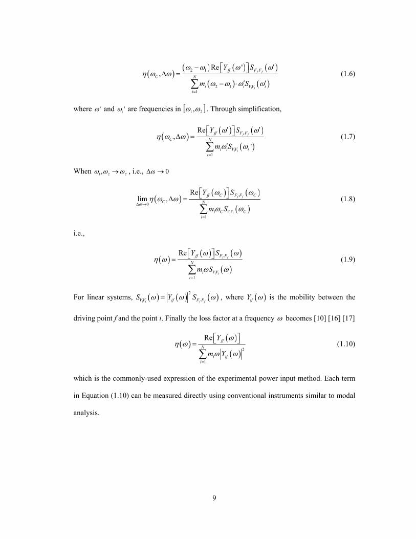
9

( )( ) ( ) ( )

( ) ( )

2 1

2 1

1

Re ', f f

i i

ff F F

C N

i i V V i

i

Y S

m S

ω ω ω ωη ω ω

ω ω ω ω=

′ − ∆ =′ ′− ⋅∑

(1.6)

where 'ω and 'i

ω are frequencies in [ ]21

,ωω . Through simplification,

( )( ) ( )

( )1

Re,

'

f f

i i

ff F F

C N

i i VV i

i

Y S

m S

ω ωη ω ω

ω ω=

′ ′ ∆ =′∑

(1.7)

When C

ωωω →21

, , i.e., 0→∆ω

( )( ) ( )

( )0

1

Relim ,

f f

i i

ff C F F C

C N

i C VV C

i

Y S

m Sω

ω ωη ω ω

ω ω∆ →

=

∆ =

∑ (1.8)

i.e.,

( )( ) ( )

( )1

Ref f

i i

ff F F

N

i VV

i

Y S

m S

ω ωη ω

ω ω=

=

∑ (1.9)

For linear systems, ( ) ( ) ( )2

i i f fVV if F FS Y Sω ω ω= , where ( )ifY ω is the mobility between the

driving point f and the point i. Finally the loss factor at a frequency ω becomes [10] [16] [17]

( )( )

( )2

1

Re ff

N

i if

i

Y

m Y

ωη ω

ω ω=

=

∑ (1.10)

which is the commonly-used expression of the experimental power input method. Each term

in Equation (1.10) can be measured directly using conventional instruments similar to modal

analysis.

10

1.3.3. Current Development of the Experimental Power Input Method

Bies and Hamid (1980) [8] measured the loss factors of a lightly damped steel plate by

both the decay method and the power input method. For the power input method

measurement, their test setup included: a shaker; a "power flow transducer" (impedance head)

to measure input power; and a number of accelerometers to measure response velocities. It

was observed that the two experimental methods yielded different results. A suggested reason

was given as “the energy distribution among modes of the system during reverberant decay

was not in steady-state equilibrium”, attributing the difference to energy dissipation

mechanisms. It was also pointed out that a very large number of accurate measurements were

required, thus suggesting automated data processing and a new generation of measurement

equipment.

Ranky and Clarkson (1983) [71] measured the loss factors of a lightly damped plate using

both the decay-rate method and the power input method. An electromagnetic coil/impedance

head/accelerometer test setup was used. Six accelerometer positions were used to calculate

the energy (which is in disagreement with the suggestion by Bies and Hamid (1980) that

many more measurement locations were needed). However, it was concluded in their paper

that “there was no significant difference between the results from the two methods as long as

the modes in the analysis band had similar loss factors”. It was also concluded that otherwise,

the log of the decay-rate record would not be a straight line and thus made it difficult to

obtain a constant loss factor.

Jacobsen (1986) [36] tested several structures including a rectangular steel box, an open

aluminum shell (moderately damped and heavily damped), a steel plate (moderately damped

and heavily damped), a steel cylindrical shell (undamped) and an aluminum beam (lightly

damped). A shaker/force transducer/accelerometer test setup was used. The kinetic energy

11

was estimated by averaging the velocity across 10 to 50 points. By observation of the test

results, Jacobsen concluded that for his method of implementation:

1) The power input method was “unsuited for examining heavily damped (η >0.1) or

very lightly damped (η <0.001) structures”. [It has been shown that heavily damped

structures can be estimated using the power input method in the current research.]

Possible reasons were given as

a) An inadequate number of measurement points were used for heavily damped

structures.

b) Minute phase errors in the two measurement channels.

2) The power input method was not good for quick survey measurements because it was

time consuming to move and position the accelerometer across many points.

3) The power input method could not be used on structures with complex shapes due to

the requirement that the structure under test should “allow a meaningful

determination of the local mass-per-point in the discrete spatial averaging”.

Plunt (1991) [66] measured a lightly-damped steel plate using both the free-decay method

and the power input method. Ten to twenty measurement positions were used. Two test

setups were investigated: 1) Hammer/accelerometer; 2) Shaker/impedance

head/accelerometer. From the comparison between the free-decay method and the power

input method results, it was concluded that the shaker setup agreed better with the free-decay

method results. In addition, a damped car floor was measured. The tested frequency range

was from 0 to 2000 Hz. Results showed loss factors as high as 0.3 in the medium frequency

range. Conclusions included:

1) The power input method could be used for complex built-up structures. It was

superior to the free-decay method when modal coupling was strong.

12

2) Loss factor results could be obtained for a wide range from 0.001 to 0.5.

3) Data acquisition could be very similar to conventional modal analysis measurement.

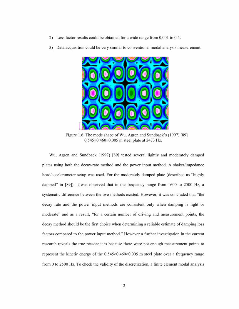
Figure 1.6 The mode shape of Wu, Agren and Sundback’s (1997) [89]

0.545×0.460×0.005 m steel plate at 2473 Hz.

Wu, Agren and Sundback (1997) [89] tested several lightly and moderately damped

plates using both the decay-rate method and the power input method. A shaker/impedance

head/accelerometer setup was used. For the moderately damped plate (described as “highly

damped” in [89]), it was observed that in the frequency range from 1600 to 2500 Hz, a

systematic difference between the two methods existed. However, it was concluded that “the

decay rate and the power input methods are consistent only when damping is light or

moderate” and as a result, “for a certain number of driving and measurement points, the

decay method should be the first choice when determining a reliable estimate of damping loss

factors compared to the power input method.” However a further investigation in the current

research reveals the true reason: it is because there were not enough measurement points to

represent the kinetic energy of the 0.545×0.460×0.005 m steel plate over a frequency range

from 0 to 2500 Hz. To check the validity of the discretization, a finite element modal analysis

13

is carried out. As shown in Figure 1.6, at 2473 Hz, the mode shape of an undamped plate is

too complex to be represented by only six measurement points. Thus, it is believed that the

difference in damping estimation is because of a lack of discretization, not because of the

damping level.

Carfagni and Pierini (1999) [17] tested highly damped steel plates, as well as conducted

numerical investigations, which are summarized in a later section. A hammer/accelerometer

setup was used. Conclusions included:

1) Manual skills of hammer tapping turned out to have an influence on the test result.

2) The excitation point position affects the test result. Edges and nodal lines should be

avoided if possible.

3) The loss factor results converge as the discretization becomes finer.

Carfagni, Citti and Pierini (1998) [18] also used a shaker to replace the hammer

excitation so that the measurement problems associated with hammer excitation could be

avoided, which is consistent with what Plunt (1991) pointed out.

Renji and Narayan (2002) [72] tested a composite sandwich plate with carbon-fiber-

reinforced polymer (CFRP) face sheets and an aluminum honeycomb core using the power

input method only. A shaker/impedance head/accelerometer test setup was used. Considering

the fact that usually the test was conducted in air, it was pointed out that the loss factors

measured were total loss factors that consisted of dissipation loss factors and radiation loss

factors. Radiation loss factors were calculated theoretically, and then subtracted from the

experimental total loss factors to get dissipation loss factors. It was claimed that “the

dissipation loss factors of the composite panel with carbon-fiber-reinforced polymer face

sheets are approximately the same as those with aluminum face sheets. No comparative study

was presented .

14

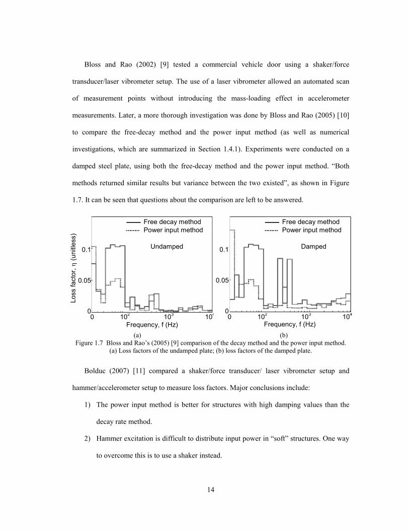
Bloss and Rao (2002) [9] tested a commercial vehicle door using a shaker/force

transducer/laser vibrometer setup. The use of a laser vibrometer allowed an automated scan

of measurement points without introducing the mass-loading effect in accelerometer

measurements. Later, a more thorough investigation was done by Bloss and Rao (2005) [10]

to compare the free-decay method and the power input method (as well as numerical

investigations, which are summarized in Section 1.4.1). Experiments were conducted on a

damped steel plate, using both the free-decay method and the power input method. “Both

methods returned similar results but variance between the two existed”, as shown in Figure

1.7. It can be seen that questions about the comparison are left to be answered.

(a) (b)

Figure 1.7 Bloss and Rao’s (2005) [9] comparison of the decay method and the power input method.

(a) Loss factors of the undamped plate; (b) loss factors of the damped plate.

Bolduc (2007) [11] compared a shaker/force transducer/ laser vibrometer setup and

hammer/accelerometer setup to measure loss factors. Major conclusions include:

1) The power input method is better for structures with high damping values than the

decay rate method.

2) Hammer excitation is difficult to distribute input power in “soft” structures. One way

to overcome this is to use a shaker instead.

0.1

0.05

0

Frequency, f (Hz) 0 10

2 10

3 10

4

Loss facto

r, η

(unitle

ss)

Free decay method

⋅⋅⋅⋅⋅⋅⋅⋅⋅⋅⋅⋅⋅⋅⋅⋅⋅⋅⋅⋅⋅⋅⋅⋅⋅⋅⋅⋅⋅⋅⋅⋅ Power input method

Free decay method

⋅⋅⋅⋅⋅⋅⋅⋅⋅⋅⋅⋅⋅⋅⋅⋅⋅⋅⋅⋅⋅⋅⋅⋅⋅⋅⋅⋅⋅⋅⋅⋅ Power input method

0.1

0.05

0

Frequency, f (Hz) 0 10

2 10

3 10

4

Undamped

Damped

15

Based on the above literature survey, it is identified that current needs in experimental

methods are:

1) Thorough studies of the experimental power input method, e.g., excitation

configuration study, discretization convergence study, etc.

2) Comparison of the experimental power input method results with analytical ones.

3) Damping estimation in an extended frequency range (from 0 to 5000Hz) to meet

emerging needs of the transportation industries [67].

4) Application of the power input method to investigate structures with particle damping

and non-uniformly damped structures, e.g., partially-covered constrained layer

damping panels.

1.4. Analytical Methods

1.4.1. Analytical Methods for Viscoelastic Damping

There has been a need for analytical damping estimation, as reflected in the statement by

Zhu, Crocker and Rao (1989) [92] that “because of the complexity of structural

configurations, different materials, interface conditions, joints, etc., damping is usually

determined by experiments”.

When computational capability was limited, closed form solutions were developed. The

usual approach is to start from Partial Differential Equations (PDEs) of motion. The first

extensive discussion of damped sandwich beams was given by Ross, Ungar and Kerwin

(1959) [74], based on a fourth-order partial differential equation. Their solution gave loss

factors for infinite-length beams or finite beams with simply supported boundary conditions.

DiTaranto (1965) [26] derived a sixth-order partial differential equation to describe the

motion of the sandwich beam, enabling the analysis of finite-length beams with boundary

16

conditions other than just simply-supported. Mead and Markus (1969) [56] refined the theory

of DiTaranto by re-deriving the partial differential equation and then extended their theory to

fixed-fixed beams.

With the appearance of computers, finite element methods started to show more

flexibility in modeling complex structures and boundary conditions as a result of enhanced

computational capability. Carne (1975) [19] developed a two-dimensional damped beam

model using MSC/NASTRAN. The base beam and the constraining layer were modeled by

offset beam elements. The middle-damping layer was modeled by rectangular shear panels.

The material properties of the damping layer were represented by a complex shear modulus.

Though the shear storage modulus and loss factor of viscoelastic materials are frequency-

dependent, they were treated as constants in modeling. Carne concluded that:

1) The necessity of a total of six boundary conditions implies that a sixth-order partial

differential equation is the lowest order that could accurately describe the motion of a

sandwich beam, consistent with what Mead (1973) [55] remarked.

2) The representation of complex shear modulus leads to a complex eigenvalue analysis

giving complex eigenvectors thus indicated that the normal modes no longer exist as

Mead and Markus (1969) concluded.

Johnson, Kienholz and Rogers (1981) [39] developed a three-dimensional plate model

using the MSC/NASTRAN program. The base plate and the constraining layer were modeled

by two-dimensional offset plate elements (QUAD/TRIA elements in MSC/NASTRAN). The

middle-damping layer was modeled by three-dimensional solid elements (HEX/PENT

elements in MSC/NASTRAN). The material properties of the middle-damping layer were all

treated as real and constant so that a standard normal-modes analysis (MSC/NASTRAN

solution 103) suffices. A Modal Strain Energy (MSE) method was also presented to calculate

17

modal loss factors from the normal-modes analysis, which is briefly described as follows.

The loss factor is defined as:

( )( )

( )1

rNr Si

i ri S

E

Eη η

=

=∑ (1.11)

where )(rη is the system’s modal loss factor at the rth mode, i

η is the material loss factor for

material i, )(r

SiE is the average strain energy in material i when the structure deforms in natural

vibration mode r, and ( )r

SE is the system’s overall strain energy in natural vibration mode r.

Then to take into account the frequency-dependent material properties, a simple empirical

correction has been given as:

( )( ) ' ( ) 2

2,

r r r

REF

G f

Gη η= (1.12)

where )'(rη is the adjusted modal loss factor for the rth mode, )(rη is the system’s modal loss

factor at the rth mode, 2,REFG is the core shear modulus used in normal modes calculation,

and ( )r

fG2

is the core shear modulus at f=r

f where r

f is the rth mode frequency calculated

with core shear modulus as 2,REFG .

Carfagni and Pierini (1999) [16] did the first numerical investigation on the power input

method to evaluate the effect that assumptions have on results. First, a system with eight

lumped masses was analyzed. It was found that the error, which was introduced by replacing

the potential energy with twice the kinetic energy at non-resonance frequencies, decreased as

the natural frequencies became closer, in other words, as modal coupling became stronger.

[Note: this feature enables the power input method to do well where the free-decay method

can not.] Further numerical investigations included modeling a flat plate for modal analysis

for the first 10 modes using ANSYS to determine experimental discretization plan. [Note: so

18

far this is the only analytical work using the power input method concept on plate-type

structures.] It was concluded that “with the number of portions being equal, the error

increased as the frequency increased”. This is because as the frequency increases, the

deflection shape of the plate becomes more complex, which makes the nodes less

representative of the vibratory features.

Bloss and Rao (2002) [9] did a parametric study by modeling spring/mass/damper

systems. It was observed that both the decay method and the power input method yielded

accurate results. But for highly damped structures, the decay method gave significantly lower

loss factors than the power input method.

To model the frequency-dependency of viscoelastic material properties, several other

finite element methods appeared, namely the Golla-Hughes-McTavish (GHM) [54] method,

the Augmented Thermodynamic Fields (ATF) [42] method and Anelastic Displacement Field

(ADF) [47] method. These methods augment the usual finite element model by introducing

internal dissipation coordinates. For example, in the GHM method, the material property data

of viscoelastic material are curve-fitted to a polynomial first, with coefficients reflecting the

material properties of the viscoelastic damping layer. The Laplace Transform is then used so

this polynomial can be incorporated into the Laplacian domain governing equations of the

structure. This way, the frequency-dependent material properties are taken into account with

the price of increased computational cost. The results of these augmented finite element

methods are concluded to be more accurate than the commonly-used modal strain energy

method proposed by Johnson, Kienholz and Rodgers (1981). However, the additional

dissipation coordinates prevent these finite element methods from using commercially

available software.

19

Based on the above literature survey, it is identified that the current gaps in analytical

methods are:

1) Modeling of the frequency-dependency of viscoelastic material properties in

constrained layer damping treatment: the commonly-used modal strain energy

method uses only constant material properties, followed by an approximate

correction.

2) Using commercially available finite element software (MSC/NASTRAN) to ease and

standardize the process, overcoming the limitation of augmented finite element

model methods caused by introducing internal dissipation coordinates.

3) Exploring new analytical procedures to estimate damping in engineering structures.

Besides the above gaps, there is also a need to compare experimental and analytical

estimation of damping over an extended frequency range.

1.4.2. Analytical Methods for Particle Damping

Due to the complex interaction involved in particle damping, a comprehensive analytical

method is not yet available [31]. Current methods can be generally categorized into three

groups:

1) Equivalent model. Papalou and Masri (1996) [63] proposed an approximate single-

particle damper model, aimed to predict the root mean square response. Nayfeh,

Verdirame and Varanasi (2002) [62] developed 3-D shell equations to model

powders as a compressible fluid with complex speed of sound for qualitative

explanation.

2) Semi-empirical methods. Friend and Kinra (2000) [33] developed an analytical

method, assuming that all particles move as a lumped mass. An “effective coefficient

20

of restitution” is adopted to minimize analytical and experimental discrepancies. Xu

(2004) [90] presented an empirical method where the damping capacity is determined

by curve-fitting based on extensive experiments.

3) Explicit Discrete Element Method (DEM). This method tracks the individual motion

of each particle [25][76]. As a result, it reveals more accurately the impact and

friction in between particles, given that the impact and friction mechanism is

accurately modeled. But, it also requires high computational cost. So, it is practical

only for a small number of particles enclosed in a few cavities.

In this research, glass microbubbles are used as the damper, considering their low density

compared to metal particles. But current methods do not offer quick quantitative damping

estimation that fits for the design of particle damping using glass microbubbles.

21

2. Structures with Viscoelastic Damping

Studies on structures with viscoelastic damping include experimental work and analytical

work. Results are presented and summarized in this chapter. The results described in this

section are published in Reference [49].

2.1. Experimental Study

Experimental setup used in this research is described first and then responses obtained

through experiments and finite element computations are compared.

2.1.1. Experimental Setup

All three commonly-used methods mentioned in Section 1.3 are applied in this research.

For the modal curve-fitting method and the power input method, a shaker is used as the

mechanical excitation, as shown in Figure 2.1(a). For the free decay method, a speaker is

used as the noise excitation, because it eliminates the shaker armature interference.

For both shaker and speaker excitation, a pseudo-random excitation signal is usually used

to generate broadband responses. Test articles are suspended by a light and soft spring to

simulate free boundary conditions. The other end of the spring is attached to a massive and

stiff frame, so vibrational energy is reflected back to the test article with minimum energy

loss at the boundary. Wolf Jr. (1984) [88] provided a rule-of-thumb for designing suspension

systems: to simulate free boundary conditions, the first rigid body mode under the constraint

of the suspension should be no more than 1/10 of the first elastic mode. For example, the

most dominant rigid body mode (the vertical translational mode) of a damped aluminum plate

22

is measured to be at 1.4 Hz, which is much less than 1/10 of the plate’s first bending mode

91Hz/10=9.1 Hz.

(a) (b)

Figure 2.1 Experimental instruments. (a) A shaker attached to the test article through a force

transducer and an aluminum connector; (b) Polytec OFV 056 laser scanning head.

The response of the test article is measured using a Polytec OFV 056 scanning laser

vibrometer, a non-contact measuring instrument, with built-in excitation signal generator, as

shown in Figure 2.1(b). STAR software is used for modal curve-fitting analysis. A typical

experimental setup is illustrated in Figure 2.2. Tests are done at room temperature,

approximately 20 °C.

Figure 2.2 A typical experimental setup in this research.

Aluminum alloy plates are chosen as test articles to simulate aerospace structures,

especially structural skin panels. Uniformly damped and non-uniformly (partially covered)

Laser vibrometer

Shaker

Stinger

Driving point

64 cm

18 cm

Force Velocity

23

damped plates are manufactured. Sandwich honeycomb composite beams and plates are also

used. The damping material used here is viscoelastic-damping polymer, 3M F9469PC. To

make sure of the good bonding between the viscoelastic material and the structure, surfaces

are cleaned before attachment and vacuum is drawn after attachment to apply a pressure to

about 1×105 Pascal.

2.1.2. Comparison of Experimental Responses with Analytical Responses

In this section, the comparison is between the measured and predicted mobility responses

of an aluminum plate with full coverage constrained layer damping. The purpose is to

compare the analytical methods validated in Section 2.2.4 with the experimental methods.

Table 2.1 Description of the plate with full coverage constrained layer damping

Material Dimensions (m) Mass (g)

Base layer CLAD 2024-T3 0.349×0.2029×0.0016002 311

Damping layer 3M F9469PC at 20°C 0.349×0.2029×0.000127 3

Constraining sheet CLAD 2024-T3 0.349×0.2029×0.000508 30

(a) (b)

Figure 2.3 Aluminum plate with full coverage constrained layer damping. (a) The plate as a test article

with scanning points defined; (b) the plate as a finite element model with the driving point illustrated.

The sandwich aluminum plate is designed and manufactured with a configuration as

shown in Table 2.1. An analytical finite element model is built to obtain analytical responses.

The base layer and the constraining layer are modeled as QUAD4 elements and the damping

0.105 m

0.0

57 m

0.2

03 m

0.349 m

24

layer is modeled as HEX8 elements. The total degrees of freedom are 5890. Please see

Appendix A for detail definitions of materials mentioned in Table 2.1.

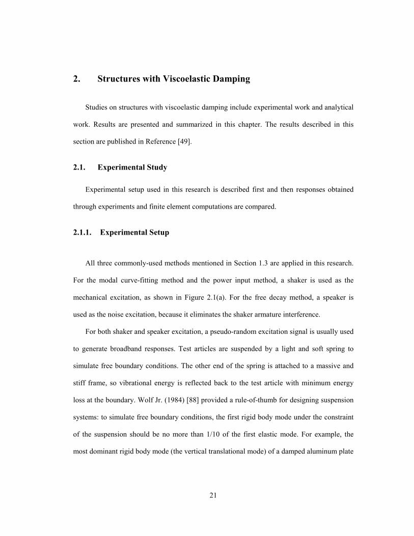
Both measured and predicted mobility responses, at two representative frequencies, are

shown in Figure 2.4. From the comparison, agreement can be seen between measured and

predicted mobility responses. Another purpose of this comparison is to illustrate the different

response characteristics of a plate in low and high frequency ranges, which is consistent with

the explanation in Reference [24] Chapter 4 that “for low-frequency measurements on a

sample of small dimensions, one may consider the test sample as a spring. At intermediate

and high frequencies, the sample then acts more like a wave-carrying distributed system. At

very high frequencies, one generally determines material data by considering the test samples

to be semi-infinite continua”.

(a) (b)

(c) (d)

Figure 2.4 Comparison of the measured and predicted responses of a damped aluminum plate. (a)

Measured mobility at 239 Hz; (b) measured mobility at 3516 Hz; (c) computed mobility at 239 Hz; (d)

computed mobility at 3519 Hz.

Measured mobility at 3516 Hz

Computed mobility at 3519 Hz

Measured mobility at

239 Hz

Computed mobility at

239 Hz

25

2.2. Analytical Study

2.2.1. Viscoelasticity

Strictly speaking, there is no pure elastic material because in reality all materials deviate

from Hooke's law in some way. Viscoelastic materials have elements of both of elastic and

viscous properties. Whereas elasticity is usually the result of bond-stretching along

crystallographic planes in an ordered solid, viscoelasticity is the result of the diffusion of

atoms or molecules inside of an amorphous material, e.g., glasses, rubbers and high polymers.

Much of the viscoelastic behavior can be described in terms of a simple combination of

elastic and viscous phenomena:

1) The elastic components can be modeled as springs of elastic constant E, given the

formula Eσ ε= , where σ is the stress; E is the elastic modulus and ε is the strain that

occurs under the given stress.

2) The viscous components can be modeled as dashpots such that the stress-strain rate

relationship can be given as d dtσ ν ε= where ν is the viscosity coefficient, and

dε/dt is the time derivative of strain.

Some common phenomena in viscoelastic materials are [45]:

1) If the stress is held constant, the strain increases with time (creep).

2) If the strain is held constant, the stress decreases with time (relaxation).

3) The effective stiffness depends on the rate of application of the load.

4) If cyclic loading is applied, hysteresis (a phase lag) occurs, along with a dissipation

of mechanical energy.

5) Acoustic waves experience attenuation.

6) Rebound of an object following an impact is less than 100%.

26

Among the common viscoelastic phenomena, two types of behavior are of major

engineering interest: transient properties (creep and relaxation) and dynamic response to

alternating load.

For transient properties, there are three commonly-used 1-DOF models (as shown in

Figure 2.5), namely, the Maxwell model, the Kelvin-Voigt model and the standard linear

solid model (a.k.a., three element model).

The Maxwell model represents viscoelastic materials by an elastic spring and a viscous

damper connected in series:

1Damper SpringTotald dd d

dt dt dt E dt

ε εε σ σν

= + = + . (2.1)

Letting

( ) ( )0 exp i t E iEσ σ ω ε′ ′′= = + , (2.2)

Equation (2.1) yields:

1

iE iE E

i

ωλωλ

′′ ′′+ =+

, (2.3)

which leads to:

2 2

2 2 2

EE

E

ω νω ν

′ =+

and 2

2 2 2

EE

E

ωνω ν

′′ =+

. (2.4)

The Kelvin-Voigt model represents viscoelastic materials by an elastic spring and viscous

damper connected in parallel:

dE

dt

εσ ε ν= + . (2.5)

The standard linear solid model represents viscoelastic materials by an elastic spring

(elastic 1 with modulus E1) and a viscous damper connected in series, then together

connected to another elastic spring (elastic 2 with modulus E2) in parallel:

27

21

2

1 2

Tot

E dE

E dtd

dt E E

ν σσ ε

νε

+ − =

+. (2.6)

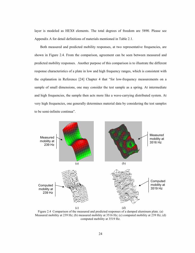
Following the same treatment presented earlier for the Maxwell model, the Kelvin-Voigt

model and the standard linear solid model yield their own expressions for moduli E′ and

E′′ , which is comparable to Equation (2.4).

(a)

(b)

(c)

Figure 2.5 Models of viscoelastic materials. (a) Maxwell model; (b) Kelvin-Voigt model; (c) standard

linear solid model.

The Maxwell model says that stress decays exponentially with time, which is accurate for

most polymers, but it is unable to predict creep. Kelvin-Voigt model is good at modeling

creep, but does not function well as to relaxation. The standard linear solid model is more

accurate than the Maxwell and Kelvin-Voigt models in modeling viscoelastic responses.

Generalized models of viscoelastic materials can be built to simulate more complex

behaviors, as shown in Figure 2.6.

Elastic Viscous

Elastic

Viscous

Elastic 1

Viscous Elastic 2

28

(a)

(b)

Figure 2.6 Generalized models of viscoelastic materials. (a) Generalized Kelvin model; (b)

Generalized Maxwell model.

The differential equation of any generalized model of the Kelvin or Maxwell type has the

form [31]

1 2 0 1 2... ...p p q q qσ σ σ ε ε ε+ + + = + + +& &&& && (2.7)

or

0 0

k km n

k kk kk k

d dp q

dt dt

σ ε

= =

=∑ ∑ (2.8)

The above equation can also be written as

σ εP = Q (2.9)

where P and Q are differential operators:

0

km

k kk

dp

dt=∑P = ,

0

kn

k kk

dq

dt=

=∑Q (2.10)

Equations (2.7), (2.8) and (2.9) are the constitutive equation which describes the

mechanical behavior of a viscoelastic material. When the constitutive equation is subjected to

29

the Laplace transformation, there results the following algebraic relation between the Laplace

transforms ( )sσ and ( )sε of stress and strain

0 0

m nk k

k k

k k

p s q sσ ε= =

=∑ ∑ (2.11)

It maybe written in the forms

( ) ( )s sσ ε⋅ ⋅P = Q (2.12)

in which ( )sP and ( )sQ are polynomials in s,

0

( )m

k

ks p s=∑P , 0

( )n

k

ks q s=∑Q (2.13)

which have the same coefficients as the differential operators P and Q.

For steady-state dynamic response to alternating load, the stress can be written as

0 0 (cos sin )i te t i tωε ε ε ω ω= = + (2.14)

When we introduce the above ε into Equation (2.8), we see that the stress must have a factor

i te ω , that is

0

i te ωσ σ= (2.15)

Equation (2.8) then reads

0 0

0 0

( ) ( )m n

k i t k i t

k k

k k

p i e q i eω ωσ ω ε ω= =

=∑ ∑ (2.16)

After cancellation of i te ω , this may be solved for the stress amplitude

0 0 0

( )

( )

k k

k

k k

k

q i i

p i i

ω ωσ ε ε

ω ω= =∑

∑Q

P (2.17)

where P and Q are the polynomials introduced before. Evidently 0σ is a complex quantity

and may be written as

0 iσ σ σ′ ′′= + (2.18)

30

whence

0 ( )(cos sin )i te i t i tωσ σ σ σ ω ω′ ′′= = + + (2.19)

After separation of real and imaginary parts

( cos sin ) ( cos sin )t t i t tσ σ ω σ ω σ ω σ ω′ ′′ ′′ ′′= − + + (2.20)

Thus, for steady-state dynamic response to alternating load, there is a phase lag between

stress and strain (Section 1.6 in reference [22] and Section 5.1 in reference [31]). For stresses

and strains that are not too large, the linear viscoelastic properties under dynamic loading can

be described by a frequency dependent complex modulus ( )*E iω . The linear relation is:

( ) ( ) ( )*, ,t E i tσ ω ω ε ω= (2.21)

Under periodic loading, both the stress and the strain are harmonic and ( )*E iω is given by

real and imaginary parts as

( ) ( ) ( )*E i E iEω ω ω′ ′′= + (2.22)

( )E ω′ and ( )E ω′′ are usually called the storage modulus and loss modulus, respectively.

In this research, the viscoelastic materials dissipate energy mostly through shear deformation.

So, the shear modulus *G replaces the Young’s modulus *E , which yields:

( ) ( ) ( )*, ,t G i tτ ω ω γ ω= (2.23)

and

( ) ( ) ( )*G i G iGω ω ω′ ′′= + (2.24)

G′ and G′′ are usually called shear storage modulus and shear loss modulus. The shear

moduli are directly provided by the manufacturer in a nomograph [1] and then incorporated

into the finite element models.

Following the above definition, the shear loss factor is:

31

G

Gη

′′=

′ (2.25)

which leads to the expression of viscoelastic shear modulus ( )* 1G G iη′= + .

2.2.2. Finite Element Modeling of Viscoelastic Materials for Steady-State

Analysis

One necessary condition for analytical studies of viscoelastically-damped structures is to

model the viscoelastic damping material accurately. The finite element method is used to

model the structure. In the MSC.Patran/Nastran 2005 r2 finite element package, viscoelastic

materials are modeled using the following method.

{ } { } { } { } tiePtxKtxBtxM ωω)()(][)(][)(][ =++ &&& (2.26)

In the frequency domain,

{ } { })()(][ 2 ωωωω PuKBiM =++− (2.27)

][][][ 21 BBB += (2.28)

where [B1] is the damping matrix generated through "CVISC" and "CDAMPi" Bulk Data

cards (damping elements); [B2] holds the damping terms generated through direct matrix

input, e.g., on the "DMIG" (Direct Matrix Input at Grid points) Bulk Data card. These would

be needed to model discrete dampers, which does not apply to this research.

In frequency response analysis, the parameters “G” and “GE” on the MATi entry do not

form a damping matrix. Instead, they form the following complex stiffness matrix:

][][])[1(][ 421 KiKKigK +++= (2.29)

where g is the overall structural damping coefficient specified through the “PARAM” Bulk

Data card. [K1] is the stiffness matrix for structural elements. This would be appropriate if all

elements had the same damping properties, which is not the case here. [K2] is the stiffness

32

terms generated through direct matrix input, e.g., "DMIG" Bulk Data card, which is not done

here. [K4] is the element damping matrix generated by the multiplication of individual

element stiffness matrices by an element damping, ge, entered on the MATi Bulk Data card;

ge is the element structural damping coefficient (“GE” on the appropriate MATi entry).

Applying Equation (2.29) on viscoelastic elements, the stiffness matrix may be written in

the form [60]:

])]}[([)](1{[][ 4KfTIggifTRgK REFREFV +++= (2.30)

where the two tables ( )fTR and ( )fTI are used to represent the real and imaginary

components of the shear modulus. Briefly the equations are [60]:

1 ( )( ) 1

REF REF

G fTR f

g G

′= −

(2.31)

1 ( )( )

REF REF

G fTI f g

g G

′′= −

(2.32)

where REFG is the reference shear modulus (G on MAT1 card); REFg is the reference

element damping (GE on MAT1 card); g is the overall structural damping (defined by

PARAM Bulk Data card). It is specified in the application manual that this formulation may

be used for direct frequency response analysis (MSC/NASTRAN 2005 r2 solution 108). This

method has been proved effective in the present research.

Literature on modeling the viscoelastic material properties in constrained layer damping

using commercially available finite element software are rarely seen. Belknap (1991) [6]

pointed out that the complex frequency-dependent shear modulus could be modeled using

MSC/NASTRAN 2005 r2 by inputting two tabular functions. However, no analytical results

were presented. Chang (1992) [20] used the same method to model a single degree-of-

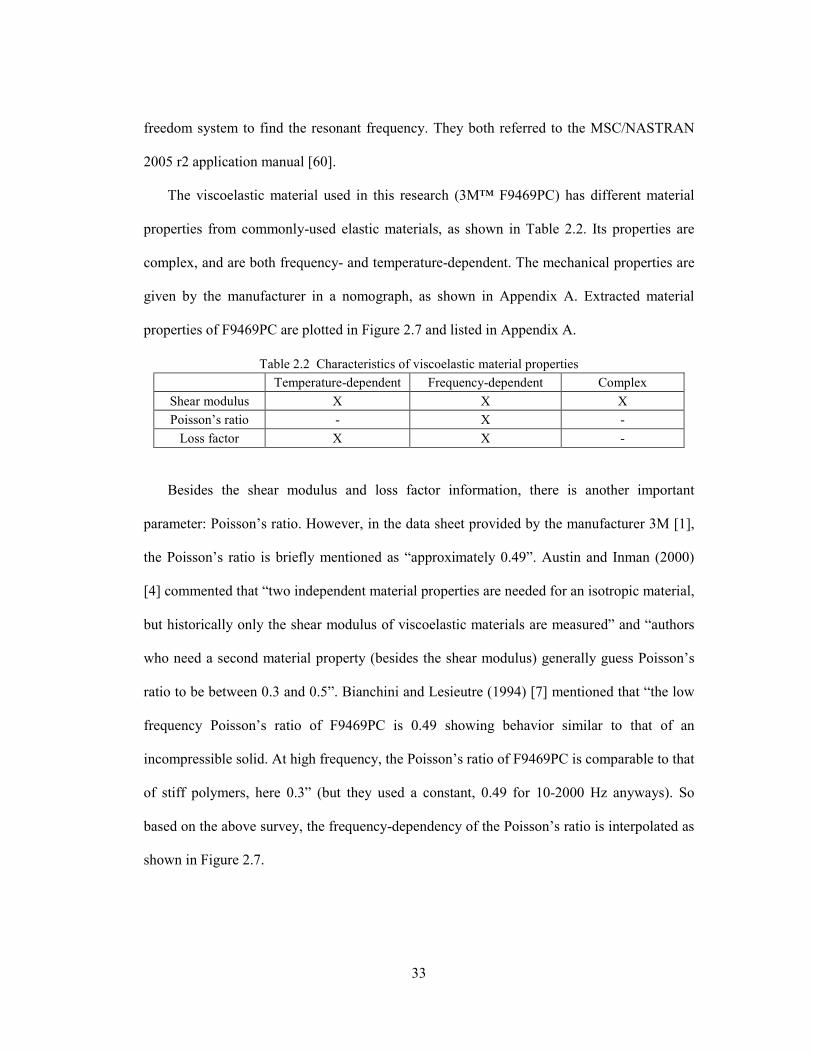
33

freedom system to find the resonant frequency. They both referred to the MSC/NASTRAN

2005 r2 application manual [60].

The viscoelastic material used in this research (3M™ F9469PC) has different material

properties from commonly-used elastic materials, as shown in Table 2.2. Its properties are

complex, and are both frequency- and temperature-dependent. The mechanical properties are

given by the manufacturer in a nomograph, as shown in Appendix A. Extracted material

properties of F9469PC are plotted in Figure 2.7 and listed in Appendix A.

Table 2.2 Characteristics of viscoelastic material properties

Temperature-dependent Frequency-dependent Complex

Shear modulus X X X

Poisson’s ratio - X -

Loss factor X X -

Besides the shear modulus and loss factor information, there is another important

parameter: Poisson’s ratio. However, in the data sheet provided by the manufacturer 3M [1],

the Poisson’s ratio is briefly mentioned as “approximately 0.49”. Austin and Inman (2000)

[4] commented that “two independent material properties are needed for an isotropic material,

but historically only the shear modulus of viscoelastic materials are measured” and “authors

who need a second material property (besides the shear modulus) generally guess Poisson’s

ratio to be between 0.3 and 0.5”. Bianchini and Lesieutre (1994) [7] mentioned that “the low

frequency Poisson’s ratio of F9469PC is 0.49 showing behavior similar to that of an

incompressible solid. At high frequency, the Poisson’s ratio of F9469PC is comparable to that

of stiff polymers, here 0.3” (but they used a constant, 0.49 for 10-2000 Hz anyways). So

based on the above survey, the frequency-dependency of the Poisson’s ratio is interpolated as

shown in Figure 2.7.

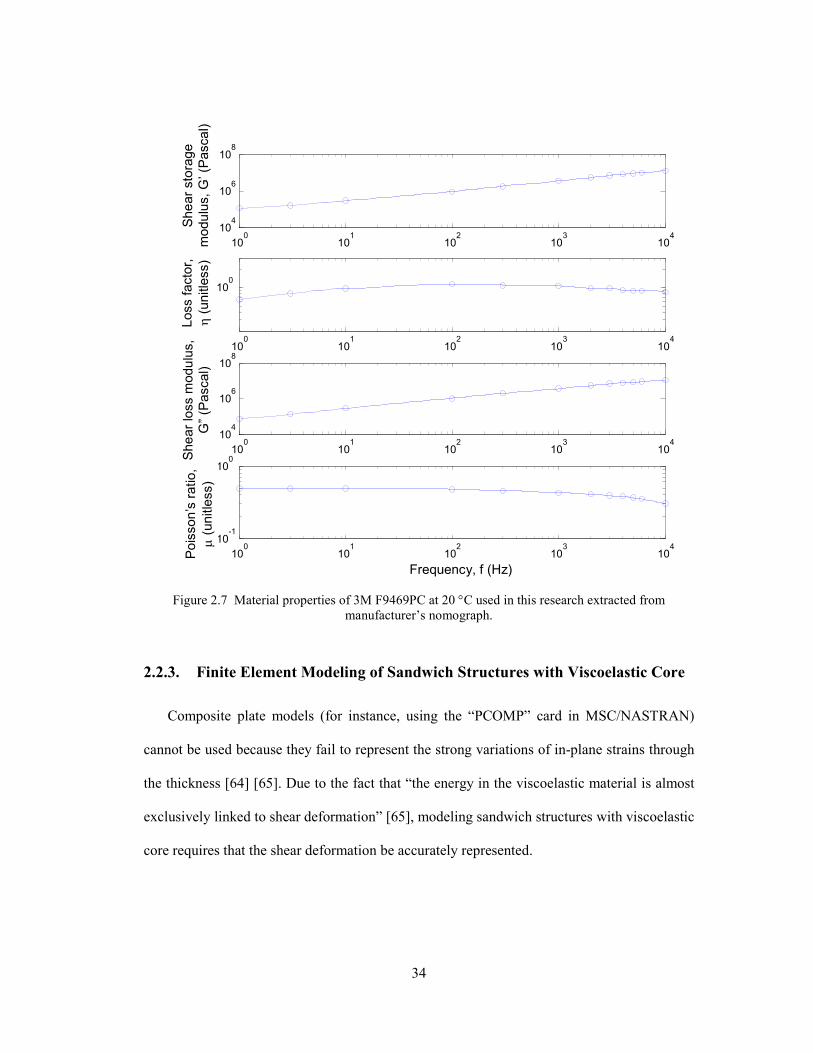
34

100

101

102

103

104

104

106

108

Shear S

tora

ge M

odulu

s (

Pa)

100

101

102

103

104

100

Loss F

acto

r

100

101

102

103

104

104

106

108

Shear Loss

Modulu

s (

Pa)

100

101

102

103

104

10-1

100

Pois

son's

Ratio

Frequency, f (Hz)

Figure 2.7 Material properties of 3M F9469PC at 20 °C used in this research extracted from

manufacturer’s nomograph.

2.2.3. Finite Element Modeling of Sandwich Structures with Viscoelastic Core

Composite plate models (for instance, using the “PCOMP” card in MSC/NASTRAN)

cannot be used because they fail to represent the strong variations of in-plane strains through

the thickness [64] [65]. Due to the fact that “the energy in the viscoelastic material is almost

exclusively linked to shear deformation” [65], modeling sandwich structures with viscoelastic

core requires that the shear deformation be accurately represented.

Shear sto

rage

modulu

s, G

’ (P

ascal)

Loss facto

r,

η (unitle

ss)

Shear lo

ss m

odulu

s,

G” (P

ascal)

Pois

son’s

ratio,

µ (unitle

ss)

Frequency, f (Hz)

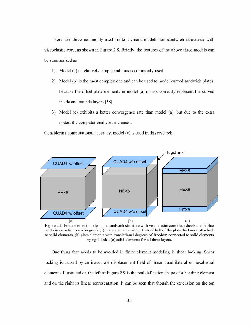
35

There are three commonly-used finite element models for sandwich structures with

viscoelastic core, as shown in Figure 2.8. Briefly, the features of the above three models can

be summarized as

1) Model (a) is relatively simple and thus is commonly-used.

2) Model (b) is the most complex one and can be used to model curved sandwich plates,

because the offset plate elements in model (a) do not correctly represent the curved

inside and outside layers [58].

3) Model (c) exhibits a better convergence rate than model (a), but due to the extra

nodes, the computational cost increases.

Considering computational accuracy, model (c) is used in this research.

(a) (b) (c)

Figure 2.8 Finite element models of a sandwich structure with viscoelastic core (facesheets are in blue

and viscoelastic core is in grey). (a) Plate elements with offsets of half of the plate thickness, attached

to solid elements; (b) plate elements with translational degrees-of-freedom connected to solid elements

by rigid links; (c) solid elements for all three layers.

One thing that needs to be avoided in finite element modeling is shear locking. Shear

locking is caused by an inaccurate displacement field of linear quadrilateral or hexahedral

elements. Illustrated on the left of Figure 2.9 is the real deflection shape of a bending element

and on the right its linear representation. It can be seen that though the extension on the top

HEX8

HEX8

HEX8

QUAD4 w/o offset

HEX8

QUAD4 w/o offset

QUAD4 w/ offset

HEX8

QUAD4 w/ offset

Rigid link

36

and the compression at the bottom are modeled, an unreal shear stress is introduced by the

linear model. This excessive shear absorbs strain energy, thus the element reaches

equilibrium with smaller nodal displacements because of shear locking. This representation

under-predicts the bending displacements and over-predicts the stiffness. To avoid shear

locking, the thickness/length ratio of solid elements should be kept above 1/5000 [42]. This

requirement is satisfied in this research, with worst case as 1/100.

(a) (b)

Figure 2.9 Real and approximate linear representations of bending deflections. (a) Real representation;

(b) linear representation.

2.2.4. Validation of Finite Element Modeling

2.2.4.1. Convergence Study

To achieve balance between accuracy and computing costs, a convergence study is

performed to determine a reasonable modeling configuration. Five models of different

discretization are built and compared against each other. Frequency and modal strain energy

ratio results of the fiftieth natural mode is presented because it is a representative plate-

bending mode and it is within the interested frequency range.

Calculations show convergence to three significant figures for both resonance frequencies

and strain energy ratios as the degrees of freedom reach 38940, as shown in Figure 2.10 and

Table 2.3. So, configuration 3 is chosen as the baseline model of current research.

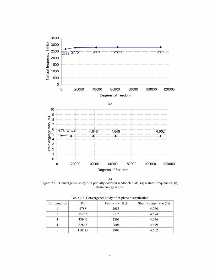
37

2683 2775 2803 2808 2808

0

500

1000

1500

2000

2500

3000

3500

0 20000 40000 60000 80000 100000 120000

Degrees of freedom

Natu

ral frequency, f (H

z)

(a)

4.76 4.674 4.646 4.649 4.652

0

1

2

3

4

5

6

7

8

9

10

0 20000 40000 60000 80000 100000 120000

Degrees of freedom

Strain

engerg

y ratio (%

)

(b)

Figure 2.10 Convergence study of a partially-covered sandwich plate. (a) Natural frequencies; (b)

strain energy ratios.

Table 2.3 Convergence study of in-plane discretization

Configuration DOF Frequency (Hz) Strain energy ratio (%)

1 4788 2683 4.760

2 15252 2775 4.674

3 38940 2803 4.646

4 62865 2808 4.649

5 110715 2808 4.652

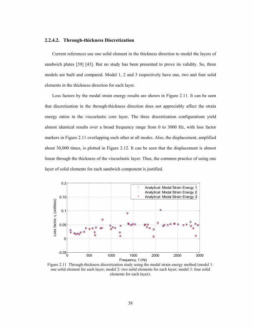
38

2.2.4.2. Through-thickness Discretization

Current references use one solid element in the thickness direction to model the layers of

sandwich plates [39] [43]. But no study has been presented to prove its validity. So, three

models are built and compared. Model 1, 2 and 3 respectively have one, two and four solid

elements in the thickness direction for each layer.

Loss factors by the modal strain energy results are shown in Figure 2.11. It can be seen

that discretization in the through-thickness direction does not appreciably affect the strain

energy ratios in the viscoelastic core layer. The three discretization configurations yield

almost identical results over a broad frequency range from 0 to 3000 Hz, with loss factor

markers in Figure 2.11 overlapping each other at all modes. Also, the displacement, amplified

about 30,000 times, is plotted in Figure 2.12. It can be seen that the displacement is almost

linear through the thickness of the viscoelastic layer. Thus, the common practice of using one

layer of solid elements for each sandwich component is justified.

0 500 1000 1500 2000 2500 3000-0.05

0

0.05

0.1

0.15

0.2

Loss facto

r, η

(unitle

ss)

Frequency, f (Hz)

Analytical: Modal Strain Energy 1



Figure 2.11 Through-thickness discretization study using the modal strain energy method (model 1:

one solid element for each layer; model 2: two solid elements for each layer; model 3: four solid

elements for each layer).

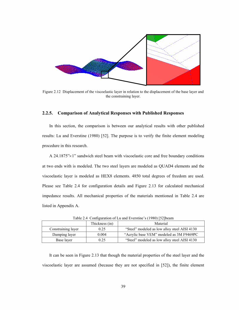
39

Figure 2.12 Displacement of the viscoelastic layer in relation to the displacement of the base layer and

the constraining layer.

2.2.5. Comparison of Analytical Responses with Published Responses

In this section, the comparison is between our analytical results with other published

results: Lu and Everstine (1980) [52]. The purpose is to verify the finite element modeling

procedure in this research.

A 24.1875”×1” sandwich steel beam with viscoelastic core and free boundary conditions

at two ends with is modeled. The two steel layers are modeled as QUAD4 elements and the

viscoelastic layer is modeled as HEX8 elements. 4850 total degrees of freedom are used.

Please see Table 2.4 for configuration details and Figure 2.13 for calculated mechanical

impedance results. All mechanical properties of the materials mentioned in Table 2.4 are

listed in Appendix A.

It can be seen in Figure 2.13 that though the material properties of the steel layer and the

viscoelastic layer are assumed (because they are not specified in [52]), the finite element

Table 2.4 Configuration of Lu and Everstine’s (1980) [52]beam

Thickness (in) Material

Constraining layer 0.25 “Steel” modeled as low alloy steel AISI 4130

Damping layer 0.004 “Acrylic base VEM” modeled as 3M F9469PC

Base layer 0.25 “Steel” modeled as low alloy steel AISI 4130

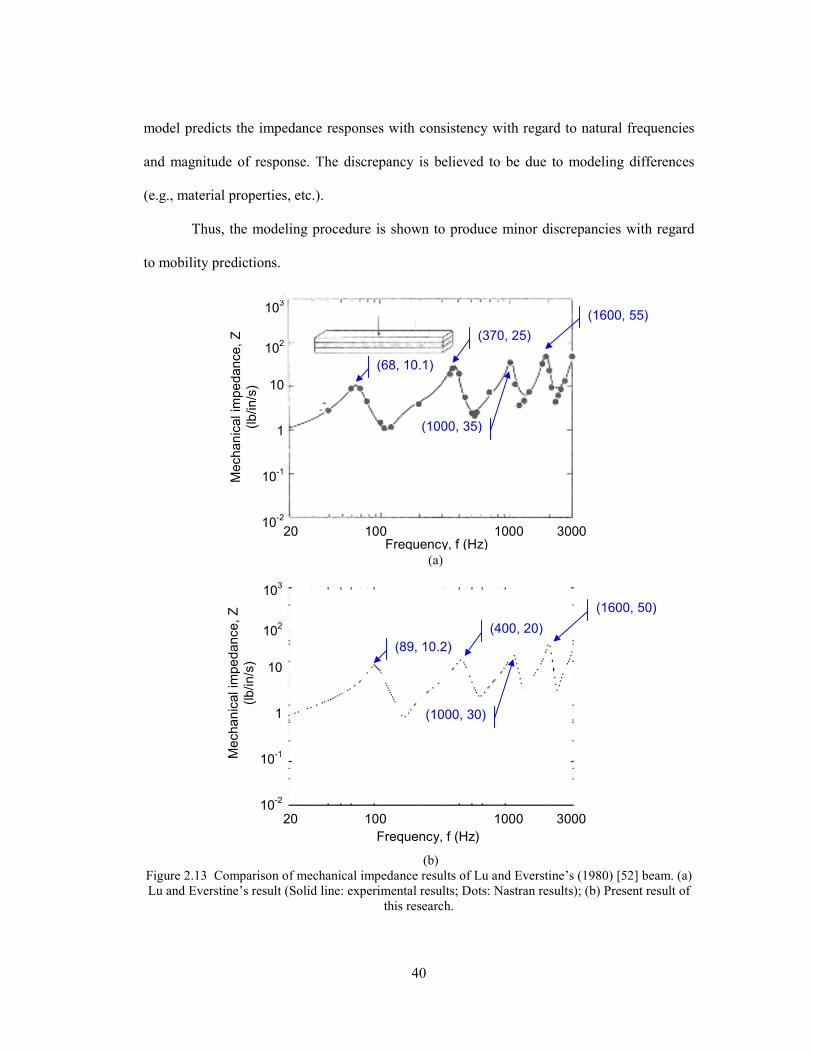
40

model predicts the impedance responses with consistency with regard to natural frequencies

and magnitude of response. The discrepancy is believed to be due to modeling differences

(e.g., material properties, etc.).

Thus, the modeling procedure is shown to produce minor discrepancies with regard

to mobility predictions.

(a)

(b)

Figure 2.13 Comparison of mechanical impedance results of Lu and Everstine’s (1980) [52] beam. (a)

Lu and Everstine’s result (Solid line: experimental results; Dots: Nastran results); (b) Present result of

this research.

103

102

10

1

10-1

10-2

20 100 1000 3000

Mechanic

al im

pedance, Z

(lb/in/s

)

Frequency, f (Hz)

Frequency, f (Hz)

Mechanic

al im

pedance, Z

(lb/in/s

)

103

102

10

1

10-1

10-2

20 100 1000 3000

(68, 10.1)

(370, 25)

(1000, 35)

(1600, 55)

(89, 10.2)

(400, 20)

(1000, 30)

(1600, 50)

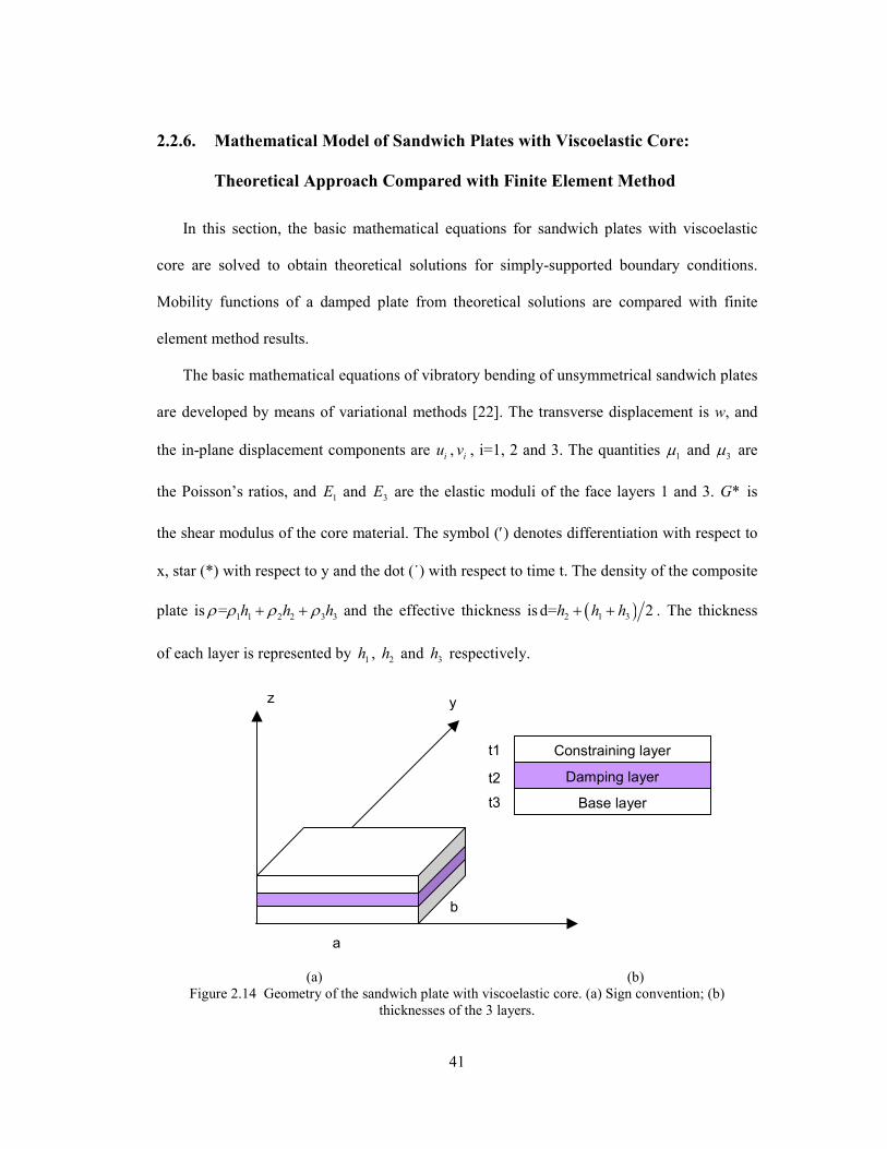
41

2.2.6. Mathematical Model of Sandwich Plates with Viscoelastic Core:

Theoretical Approach Compared with Finite Element Method

In this section, the basic mathematical equations for sandwich plates with viscoelastic

core are solved to obtain theoretical solutions for simply-supported boundary conditions.

Mobility functions of a damped plate from theoretical solutions are compared with finite

element method results.

The basic mathematical equations of vibratory bending of unsymmetrical sandwich plates

are developed by means of variational methods [22]. The transverse displacement is w, and

the in-plane displacement components are i

u ,i

v , i=1, 2 and 3. The quantities 1µ and 3µ are

the Poisson’s ratios, and 1E and 3E are the elastic moduli of the face layers 1 and 3. *G is

the shear modulus of the core material. The symbol (′) denotes differentiation with respect to

x, star (*) with respect to y and the dot (˙) with respect to time t. The density of the composite

plate is 1 1 2 2 3 3= h h hρ ρ ρ ρ+ + and the effective thickness is ( )2 1 3d= 2h h h+ + . The thickness

of each layer is represented by 1h , 2h and 3h respectively.

(a) (b)

Figure 2.14 Geometry of the sandwich plate with viscoelastic core. (a) Sign convention; (b)

thicknesses of the 3 layers.

z y

a

b

Constraining layer

Damping layer

Base layer

t1

t2

t3

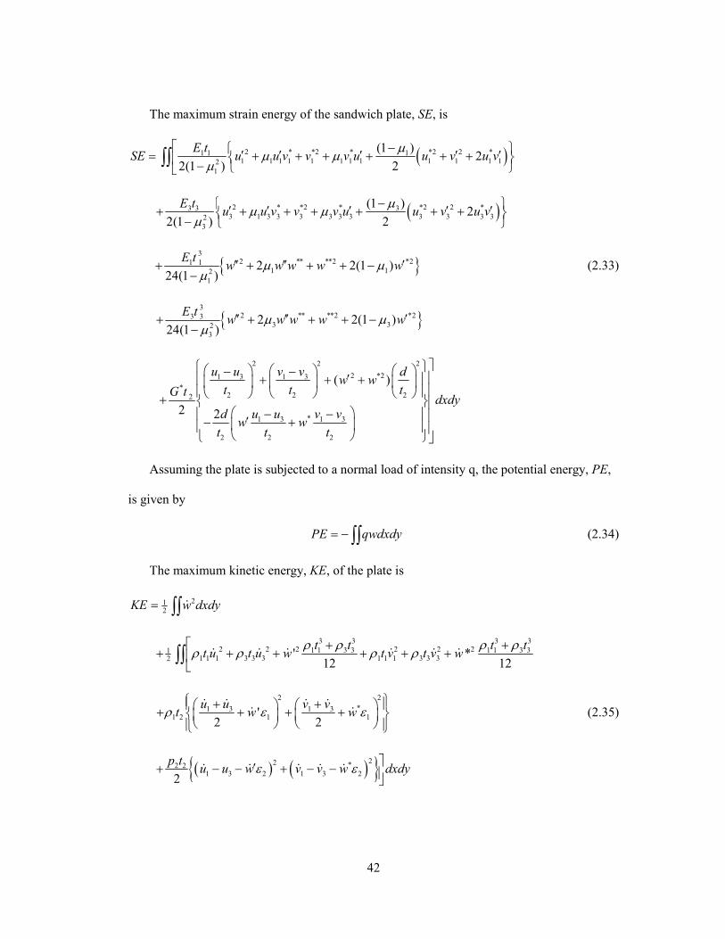
42

The maximum strain energy of the sandwich plate, SE, is

( )2 * *2 * *2 2 *1 1 11 1 1 1 1 1 1 1 1 1 1 12

1

(1 )2

2(1 ) 2

E tSE u u v v v u u v u v

µµ µ

µ − ′ ′ ′ ′ ′= + + + + + + −

∫∫

( )2 * *2 * *2 2 *3 3 33 1 3 3 3 3 3 3 3 3 3 32

3

(1 )2

2(1 ) 2

E tu u v v v u u v u v

µµ µ

µ− ′ ′ ′ ′ ′+ + + + + + +

−

{ }3

2 ** **2 *21 11 12

1

2 2(1 )24(1 )

E tw w w w wµ µ

µ′′ ′′ ′+ + + + −

− (2.33)

{ }3

2 ** **2 *23 33 32

3

2 2(1 )24(1 )

E tw w w w wµ µ

µ′′ ′′ ′+ + + + −

−

2 2 2

2 *21 3 1 3

*2 2 22

*1 3 1 3

2 2 2

( )

2 2

u u v v dw w

t t tG tdxdy

d u u v vw w

t t t

− − ′ + + + +

− − ′− +

Assuming the plate is subjected to a normal load of intensity q, the potential energy, PE,

is given by

PE qwdxdy= −∫∫ (2.34)

The maximum kinetic energy, KE, of the plate is

212

KE w dxdy= ∫∫ &

3 3 3 3

2 2 2 2 2 21 1 3 3 1 1 3 311 1 1 3 3 3 1 1 1 3 3 32

' *12 12

t t t tt u t u w t v t v w

ρ ρ ρ ρρ ρ ρ ρ + +

+ + + + + +

∫∫ & & & & & &

2 2

*1 3 1 31 2 1 1'

2 2

u u v vt w wρ ε ε + + + + + +

& & & && & (2.35)

( ) ( ){ }22 *2 21 3 2 1 3 2

2

p tu u w v v w dxdyε ε ′+ − − + − − & & & & &

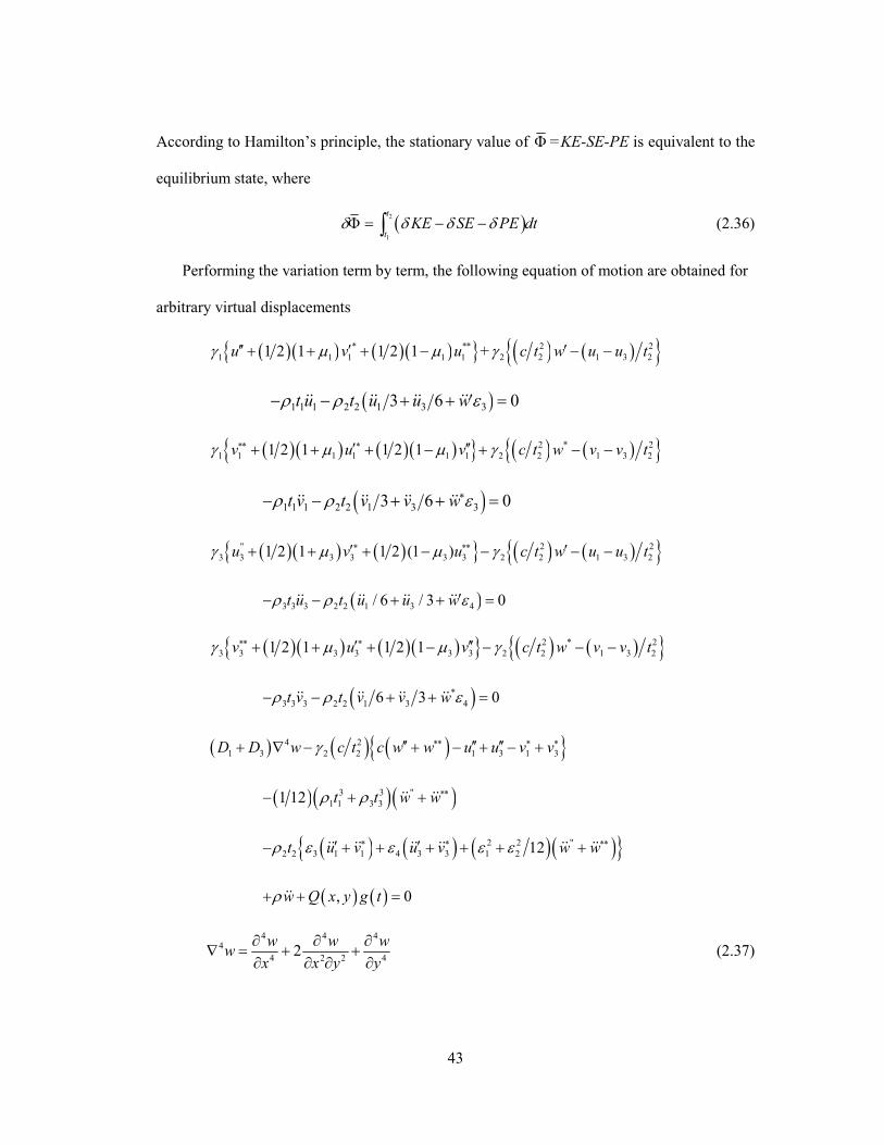
43

According to Hamilton’s principle, the stationary value of Φ =KE-SE-PE is equivalent to the

equilibrium state, where

( )2

1

t

tKE SE PE dtδ δ δ δΦ = − −∫ (2.36)

Performing the variation term by term, the following equation of motion are obtained for

arbitrary virtual displacements

( )( ) ( )( ){ }* **

1 1 1 1 11 2 1 1 2 1u v uγ µ µ′′ ′+ + + − + )( ( ){ }2 2

2 2 1 3 2c t w u u tγ ′ − −

( )1 1 1 2 2 1 3 33 6 0t u t u u wρ ρ ε′− − + + =&& && && &&

( )( ) ( )( ) }{ ( ) ( ){ }2 * 2

1 1 1 1 1 1 2 2 1 3 21 2 1 1 2 1v u v c t w v v tγ µ µ γ∗∗ ∗′ ′′+ + + − + − −

( )1 1 1 2 2 1 3 33 6 0t v t v v wρ ρ ε∗− − + + =&& && && &&

( )( ) ( ){ } ( ) ( ){ }'' 2 2

3 3 3 3 3 3 2 2 1 3 21 2 1 1 2 (1 )u v u c t w u u tγ µ µ γ∗ ∗∗′ ′+ + + − − − −

( )3 3 3 2 2 1 3 4/ 6 / 3 0t u t u u wρ ρ ε′− − + + =&& && && &&

( )( ) ( )( ){ } ( ) ( ){ }2 * 2

3 3 3 3 3 3 2 2 1 3 21 2 1 1 2 1v u v c t w v v tγ µ µ γ∗∗ ∗′ ′′+ + + − − − −

( )*

3 3 3 2 2 1 3 46 3 0t v t v v wρ ρ ε− − + + =&& && && &&

( ) ( ) ( ){ }4 2

1 3 2 2 1 3 1 3D D w c t c w w u u v vγ ∗∗ ∗ ∗′′ ′′ ′′+ ∇ − + − + − +

( )( )( )3 3 "

1 1 3 31 12 t t w wρ ρ ∗∗− + +&& &&

( ) ( ) ( )( ){ }2 2 "

2 2 3 1 1 4 3 3 1 2 12t u v u v w wρ ε ε ε ε∗ ∗ ∗∗′ ′− + + + + + +&& && && && && &&

( ) ( ), 0w Q x y g tρ+ + =&&

4 4 44

4 2 2 42

w w ww

x x y y

∂ ∂ ∂∇ = + +

∂ ∂ ∂ ∂ (2.37)

44

( )( )3 3 11 12 2t tε = −

( )( )2 1 31 2 2c t t t= + + , ( )21i i iE tγ µ= − , i = 1, 3, 2 2 2

G tγ =

( )( )4 3 11 12 2t tε = − , ( )1 3 1 4t tε = − , ( )2 1 3 2t tε = +

( )3

2,

12 1

i ii

i

E tD

µ=

− i = 1,3, 332211 ttt ρρρρ ++= (2.38)

In deriving the equations of motion, the following assumptions are made:

1) A plane transverse to the middle plane before bending remains plane and

perpendicular to the middle plane after bending

2) Transverse displacement at a section does not vary along thickness.

3) All displacements are small.

4) There is perfect continuity at the interfaces and no slip occurs.

5) The extension effect in the core is ignored and stresses in the core are considered

negligible.

For the viscoelastic core, the complex moduli are

( )2 2 21G G iη∗ = + , ( )2 2 21E E iη∗ = + (2.39)

For simply supported boundary conditions, it is assumed that

1 1

1 1

cos sin sinmn

m n

m x n yu U t

a b

π πω

∞ ∞

= =

=∑∑

3 3

1 1

cos sin sinmn

m n

m x n yu U t

a b

π πω

∞ ∞

= =

=∑∑

1 1

1 1

sin cos sinmn

m n

m x n yv V t

a b

π πω

∞ ∞

= =

=∑∑ (2.40)

3 3

1 1

sin cos sinmn

m n

m x n yv V t

a b

π πω

∞ ∞

= =

=∑∑

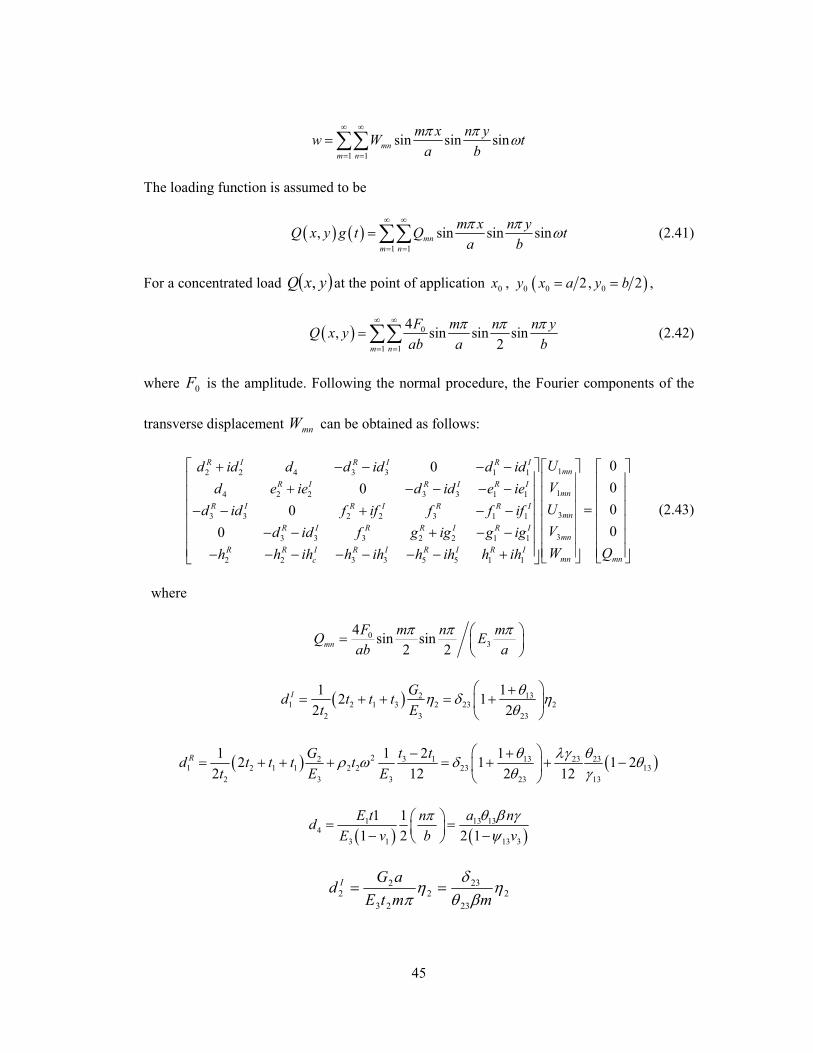
45

1 1

sin sin sinmn

m n

m x n yw W t

a b

π πω

∞ ∞

= =

=∑∑

The loading function is assumed to be

( ) ( )1 1

, sin sin sinmn

m n

m x n yQ x y g t Q t

a b

π πω

∞ ∞

= =

=∑∑ (2.41)

For a concentrated load ( )yxQ , at the point of application 0x , 0y ( )0 02, 2x a y b= = ,

( ) 0

1 1

4, sin sin sin

2m n

F m n n yQ x y

ab a b

π π π∞ ∞

= =

=∑∑ (2.42)

where 0F is the amplitude. Following the normal procedure, the Fourier components of the

transverse displacement mnW can be obtained as follows:

12 2 4 3 3 1 1

14 2 2 3 3 1 1

33 3 2 2 3 1 1

33 3 3 2 2 1 1

2 2 3 3 5 5 1 1

0

0

0

0

R I R I R Imn

R I R I R Imn

R I R I R R Imn

R I R R I R Imn

R R I R I R I R Imnc

Ud id d d id d id

Vd e ie d id e ie

Ud id f if f f if

Vd id f g ig g ig

Wh h ih h ih h ih h ih

+ − − − − + − − − − − − + − −

− − + − − − − − − − − − +

0

0

0

0

mnQ

=

(2.43)

where

03

4sin sin

2 2mn

F m n mQ E

ab a

π π π =

( ) 2 131 2 1 3 2 23 2

2 3 23

1 12 1

2 2

I Gd t t t

t E

θη δ η

θ +

= + + = +

( ) ( )22 3 1 13 23 231 2 1 1 2 2 23 13

2 3 3 23 13

1 1 2 12 1 1 2

2 12 2 12

R G t td t t t t

t E E

θ λγ θρ ω δ θ

θ γ − +

= + + + = + + −

( ) ( )1 13 13

4

3 1 13 3

1 1

1 2 2 1

E t n a nd

E v b v

π θ β γψ

= = − −

2

23

23

2

23

22 η

βθδ

ηπ mmtE

aGd I ==

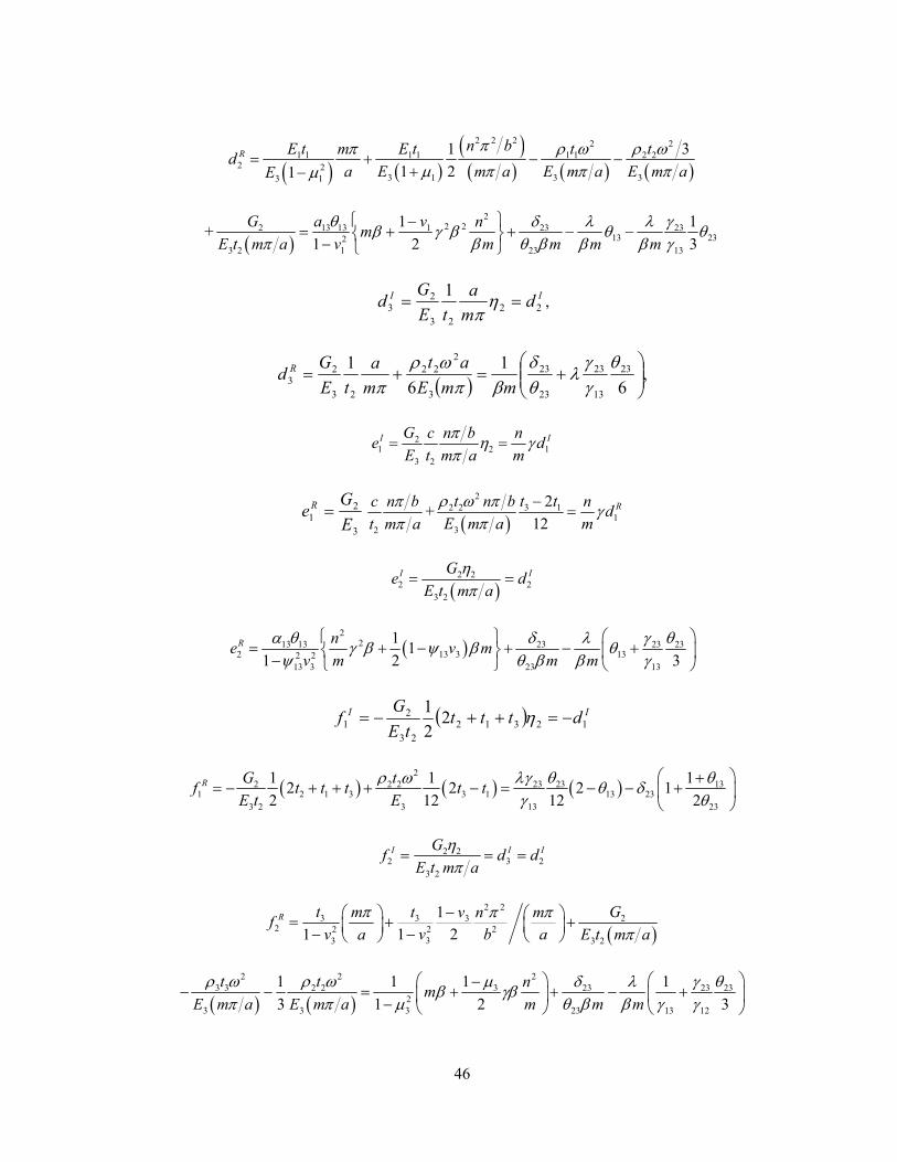
46

( ) ( )( )( ) ( ) ( )

2 2 2 2 2

1 1 1 1 1 1 2 22 2

3 1 3 33 1

1 3

1 21

Rn bE t m E t t t

da E m a E m a E m aE

ππ ρ ω ρ ωµ π π πµ

= + − −+−

+( )

22 22 13 13 1 23 23

13 232

3 2 1 23 13

1 1

1 2 3

G a v nm

E t m a v m m m m

θ δ λ λ γβ γ β θ θ

π β θ β β β γ −

= + + − − −

II dm

a

tE

Gd 22

23

23

1== η

π,

( ),

6

1

6

1 23

13

23

23

23

3

2

22

23

23

+=+=

θγγ

λθδ

βπωρ

π mmE

at

m

a

tE

Gd R

21 2 1

3 2

I IG c n b ne d

E t m a m

πη γ

π= =

3

21

E

GeR =

2

c n b

t m a

ππ

+( )

2

2 2 3 11

3

2

12

Rt n b t t nd

E m a m

ρ ω πγ

π−

=

( )2 2

2 2

3 2

I IGe d

E t m a

ηπ

= =

( )2

213 13 23 23 232 13 3 132 2

13 3 23 13

11

1 2 3

R ne v m

v m m m

α θ δ λ γ θγ β ψ β θ

ψ θ β β γ

= + − + − + −

( ) II dttttE

Gf 12312

23

21 2

2

1−=++−= η

( ) ( ) ( )2

2 2 2 23 23 131 2 1 3 3 1 13 23

3 2 3 13 23

1 1 12 2 2 1

2 12 12 2

R G tf t t t t t

E t E

ρ ω λγ θ θθ δ

γ θ +

= − + + + − = − − +

2 22 3 2

3 2

I I IGf d d

E t m a

ηπ

= = =

( )

2 2

3 23 32 2 22

33 3 2

1

1 21

R t m Gt v n mf

v b av a E t m a

π π ππ

− = + + −−

( ) ( )

2 2 2

3 3 2 2 3 23 23 23

2

3 3 3 23 13 12

1 1 1 1

3 1 2 3

t t nm

E m a E m a m m m

ρ ω ρ ω µ δ λ γ θβ γβ

π π µ θ β β γ γ −

− − = + + − + −

47

( )21 2 1 3 2 1 1

3 2

12

2

I I IG n nn mg t t t f d

b aE t m m

π πη γ γ = − + + = = −

( )2

2 2 2 31 2 1 3 1

3 2 3

1 2 12

2 12

R RG t n t nn mg t t t f

b aE t E m a b m

ρ ω ππ πγ

π− = − + + + =

2 2

I Ig d=

22 3 23 23 23

2 2

3 23 13 13

1 1

1 2 3

R ng m

m m m m

µ δ λ λ γ θβγ β

µ θ β γ β γ β −

= + + − − −

( )22 2 1 3 2 1

3 2

12

2

I IGh t t t d

E tη= + + =

( ) ( )2

2 2 22 2 1 3 3 1 1

3 2 3

1 12 2

2 12

R RG th t t t t t d

E t E

ρ ω= + + + − =

( )2

2 2 2 3 14 2 1 3 1

3 2 3

1 22

2 12

R RG t n t tn mh t t t e

b aE t E m a b

ρ ω ππ ππ

− = + + + =

24

3 2

1

2

I Gh

E t= ( )2 1 32

n mt t t

b a

π π + +

2 1

Ieη =

III dfctE

Gh 112

23

23 −==−= η

,12

21

132

3

22

23

23

RR ftt

E

tc

tE

Gh =

−+−= ωρ

25 2 1

3 2

I IG n mh c g

b aE t

π πη = − =

2

2 2 2 3 15 1

3 2 3

2

/ 12

R RG t n t tn mh c g

b aE t E m a b

ρ ω ππ ππ

− = − + =

22

2 135 23 2 232

23

11 1

2

I nh m

m

θβ γ δ η θ

θ +

= + +

48

( )

23 2 4 2

3 3 2 4 213 13 23 131 232 4 2 2 22

2313 3

11 2 1 1

212 1

R n n nh m

m m m m

α θ θ θβ γ γ γ δ

β θψ µ

+ = + + + + + −

( )2 2

2 223 2313 23 13 13 13 232

13 13 13 13

1 1 11 1

12

m n

m m

β γ γ γλ θ θ θ θ θ θ

γ γ β γ γ − + + + + − + + +

(2.44)

Also

2 2

1 3 3t Eλ ρ ω=

13 1 3ψ µ µ=

13 1 3t tθ =

23 2 3t tθ =

13 1 3γ ρ ρ=

13 1 3E Eα =

3t aβ π=

a bγ =

23 2 3G Eδ = (2.45)

A damped sandwich steel plate is used as an example, as shown in Figure 2.15.

Theoretical solutions as driving point mobilities are obtained from the procedure described

above. Twenty five expansion terms are used to calculate the displacements. A finite element

model is built and MSC/Nastran 2005 r2 direct frequency response solution 108 is used to

compute mobilities at the driving point. The dimensions of the simply-supported sandwich

plate are 14 in×14 in. HEX8 elements are used for all three layers. Materials and thicknesses

are listed in Table 2.5. Please see Appendix A for detailed mechanical properties defined in

the finite element model.

49

Table 2.5 Description of the steel sandwich plate with viscoelastic core for theoretical and finite

element method comparison

Material Thickness (in)

Base layer Steel AISI 4130 0.125

Damping layer 3M F9469PC at 20°C 0.006

Constraining layer Steel AISI 4130 0.125

Figure 2.15 Finite element model of the steel sandwich plate with viscoelastic core.

Mobility functions at the driving point are chosen to be compared because they help

represent the input power in the analytical power input method, which a new analytical

damping estimation procedure introduced in a later section (Section 2.2.7) uses. Mobility

functions obtained from both the theoretical equations and finite element model are compared

in Figure 2.16. General agreement is noted on modal frequencies and mobility magnitudes,

with discrepancy diminishing with frequency. As discussed later, damping estimation at low

frequency is systemically problematic. Differences of the two results are believed to be that in

the finite element model only one layer of nodes can be defined as simply-supported. But

there are four layers of nodes for this sandwiched plate modeled with three layers of HEX8

solid elements. Choosing only one layer of the nodes in the finite element model does not

strictly agree with the simply-supported boundary condition as defined in the theoretical

equations. [However, free boundary conditions are used for all later examples in this

Driving point

14 inch

14 inch

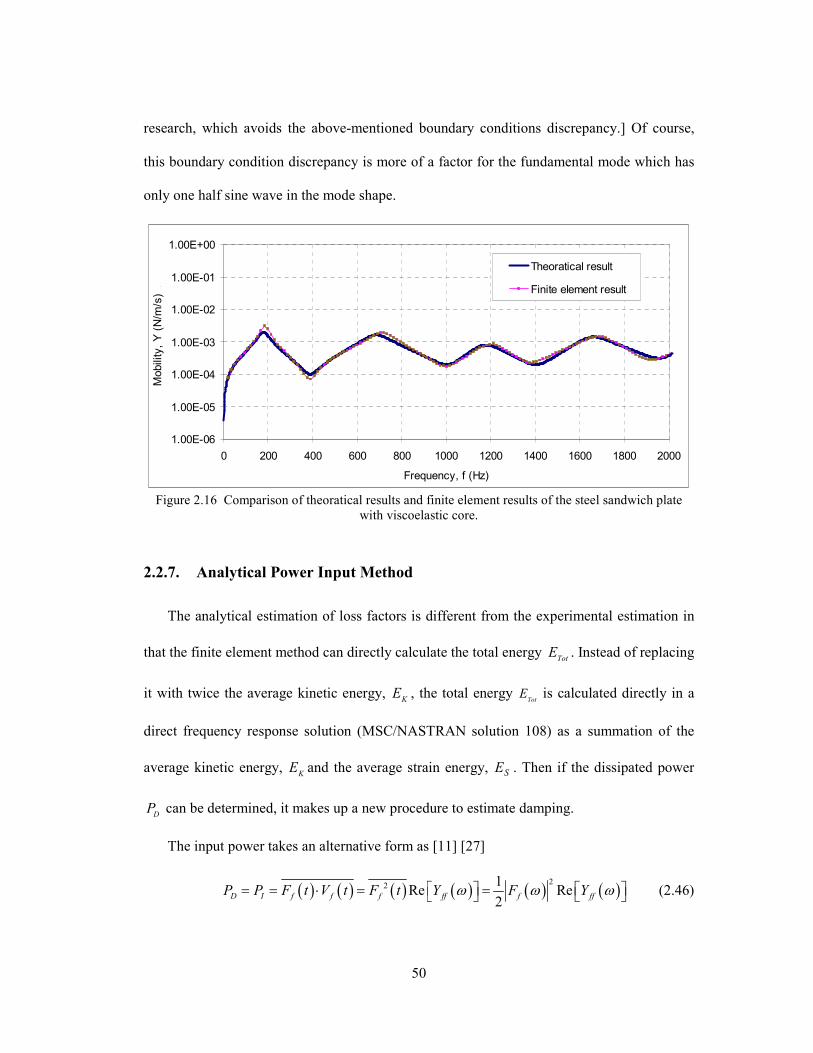
50

research, which avoids the above-mentioned boundary conditions discrepancy.] Of course,

this boundary condition discrepancy is more of a factor for the fundamental mode which has

only one half sine wave in the mode shape.

1.00E-06

1.00E-05

1.00E-04

1.00E-03

1.00E-02

1.00E-01

1.00E+00

0 200 400 600 800 1000 1200 1400 1600 1800 2000

Frequency, f (Hz)

Mobili

ty, Y (N

/m/s

) .

Theoratical result

Finite element result

Figure 2.16 Comparison of theoratical results and finite element results of the steel sandwich plate

with viscoelastic core.

2.2.7. Analytical Power Input Method

The analytical estimation of loss factors is different from the experimental estimation in

that the finite element method can directly calculate the total energy Tot

E . Instead of replacing

it with twice the average kinetic energy, K

E , the total energy Tot

E is calculated directly in a

direct frequency response solution (MSC/NASTRAN solution 108) as a summation of the

average kinetic energy, K

E and the average strain energy, SE . Then if the dissipated power

DP can be determined, it makes up a new procedure to estimate damping.

The input power takes an alternative form as [11] [27]

( ) ( ) ( ) ( ) ( ) ( )2

2 1Re Re

2D I f f f ff f ffP P F t V t F t Y F Yω ω ω = = ⋅ = = (2.46)

51

where ( )ωf

F is the Fourier transform of ( )tFf

. In addition, the driving point mobility )(ωff

Y

can be calculated in the finite element method too. Thus, the loss factor can be written as

( ) ( )

( )

21Re

2f ff

S K

F Y

E E

ω ωη

ω

=

+ (2.47)

So from the above equation, a new procedure of estimating loss factors is proposed [49].

Moreover, the frequency-dependency of the viscoelastic material is taken into account by the

method described in Section 2.2.1. Examples of loss factor estimation of different damping

configurations are included in later sections.

2.2.8. Validation of Analytical Power Input Method

To check the validity of the new analytical procedure, a test finite element model is built

and the loss factor is computed. A rectangular plate under a point excitation at the center is

given dimensions, material properties and boundary conditions consistent with structural

panels found in passenger enclosures, with a constant loss factor as 0.1. The plate is modeled

as a 0.36×0.24 m, aluminum alloy 2024-T3 plate (See Appendix A for detailed definition of

material properties in the finite element model.) with free boundary conditions. QUAD4

elements are used with total degrees of freedom as 12505. Then MSC/NASTRAN 2005 r2

direct frequency response solution 108 is computed to obtain the mobility function at the

driving point, the average strain energy, and the average kinetic energy of the system at each

excitation frequency. Then Equation (2.47) is applied to estimate loss factors. The results are

shown in Figure 2.17.

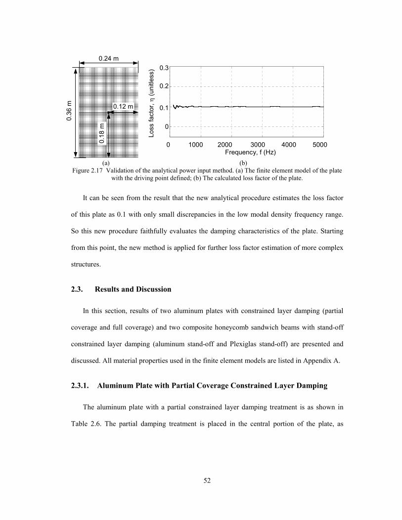
52

0 1000 2000 3000 4000 5000

0

0.1

0.2

Loss facto

rFrequency, Hz

(a) (b)

Figure 2.17 Validation of the analytical power input method. (a) The finite element model of the plate

with the driving point defined; (b) The calculated loss factor of the plate.

It can be seen from the result that the new analytical procedure estimates the loss factor

of this plate as 0.1 with only small discrepancies in the low modal density frequency range.

So this new procedure faithfully evaluates the damping characteristics of the plate. Starting

from this point, the new method is applied for further loss factor estimation of more complex

structures.

2.3. Results and Discussion

In this section, results of two aluminum plates with constrained layer damping (partial

coverage and full coverage) and two composite honeycomb sandwich beams with stand-off

constrained layer damping (aluminum stand-off and Plexiglas stand-off) are presented and

discussed. All material properties used in the finite element models are listed in Appendix A.

2.3.1. Aluminum Plate with Partial Coverage Constrained Layer Damping

The aluminum plate with a partial constrained layer damping treatment is as shown in

Table 2.6. The partial damping treatment is placed in the central portion of the plate, as

0.3

0.2

0.1

0

0 1000 2000 3000 4000 5000 Frequency, f (Hz)

Loss facto

r, η

(unitle

ss)

0.24 m

0.3

6 m

0.12 m 0.1

8 m

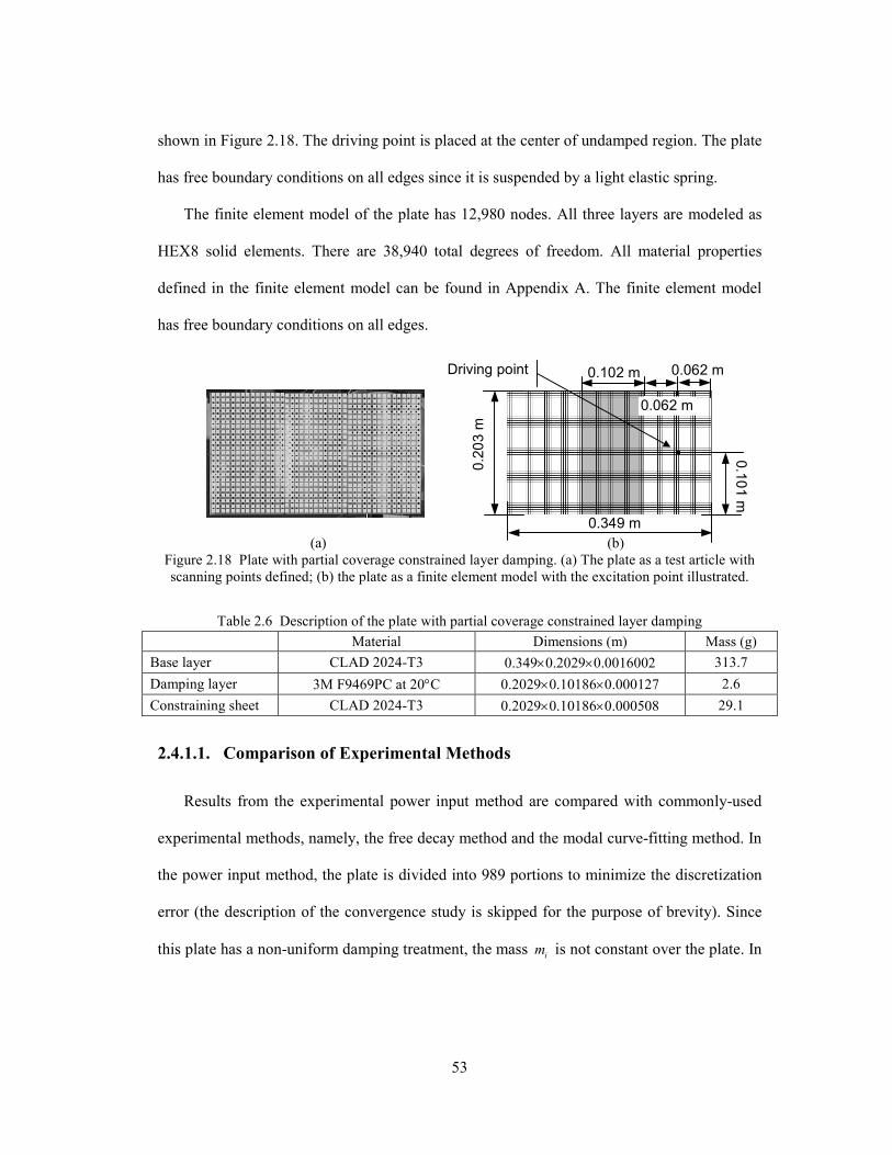
53

shown in Figure 2.18. The driving point is placed at the center of undamped region. The plate

has free boundary conditions on all edges since it is suspended by a light elastic spring.

The finite element model of the plate has 12,980 nodes. All three layers are modeled as

HEX8 solid elements. There are 38,940 total degrees of freedom. All material properties

defined in the finite element model can be found in Appendix A. The finite element model

has free boundary conditions on all edges.

(a) (b)

Figure 2.18 Plate with partial coverage constrained layer damping. (a) The plate as a test article with

scanning points defined; (b) the plate as a finite element model with the excitation point illustrated.

Table 2.6 Description of the plate with partial coverage constrained layer damping


Base layer CLAD 2024-T3 0.349×0.2029×0.0016002 313.7

Damping layer 3M F9469PC at 20°C 0.2029×0.10186×0.000127 2.6

Constraining sheet CLAD 2024-T3 0.2029×0.10186×0.000508 29.1

2.4.1.1. Comparison of Experimental Methods

Results from the experimental power input method are compared with commonly-used

experimental methods, namely, the free decay method and the modal curve-fitting method. In

the power input method, the plate is divided into 989 portions to minimize the discretization

error (the description of the convergence study is skipped for the purpose of brevity). Since

this plate has a non-uniform damping treatment, the mass i

m is not constant over the plate. In

0.062 m

0.1

01 m

0.2

03 m

0.349 m

0.102 m

0.062 m

Driving point

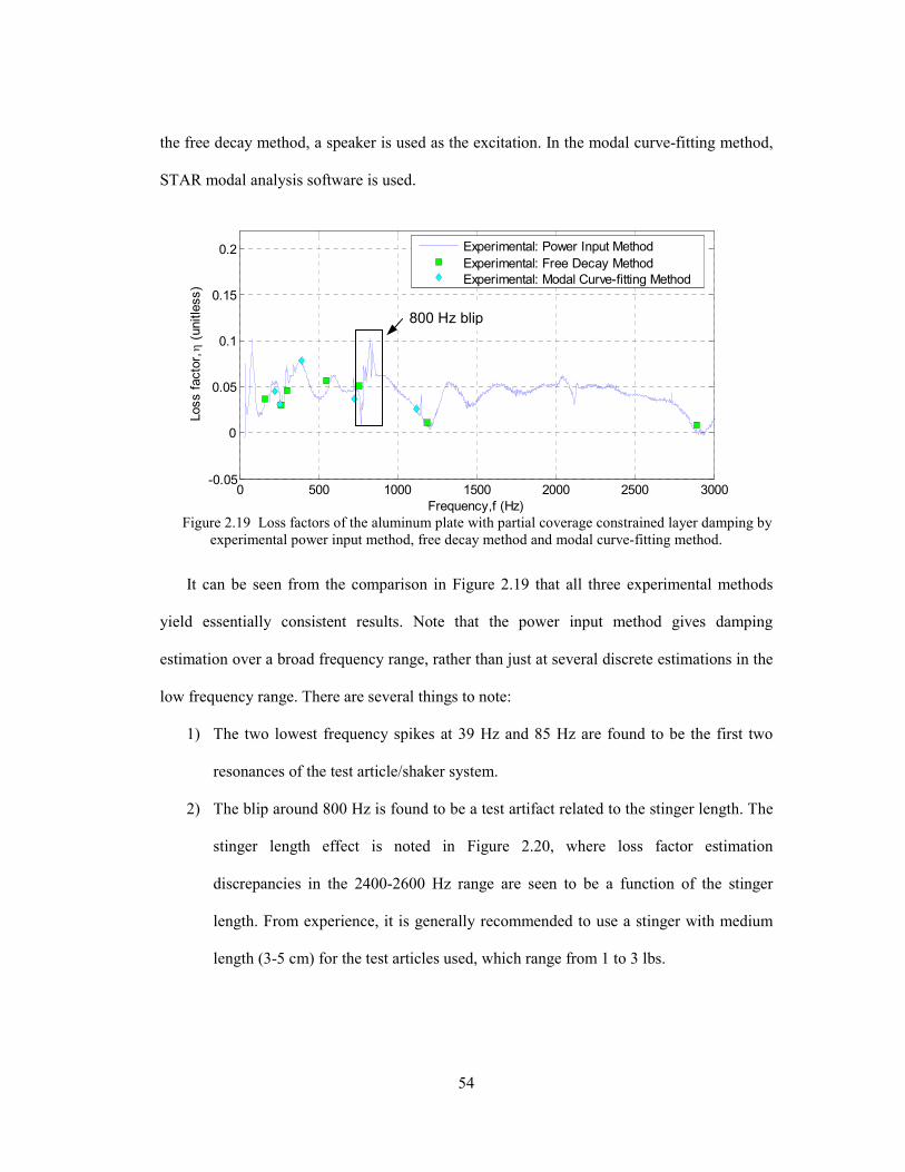
54

the free decay method, a speaker is used as the excitation. In the modal curve-fitting method,

STAR modal analysis software is used.

0 500 1000 1500 2000 2500 3000-0.05

0

0.05

0.1

0.15

0.2

Loss facto

r, η

(unitle

ss)

Frequency,f (Hz)

Experimental: Power Input Method

Experimental: Free Decay Method

Experimental: Modal Curve-fitting Method

Figure 2.19 Loss factors of the aluminum plate with partial coverage constrained layer damping by

experimental power input method, free decay method and modal curve-fitting method.

It can be seen from the comparison in Figure 2.19 that all three experimental methods

yield essentially consistent results. Note that the power input method gives damping

estimation over a broad frequency range, rather than just at several discrete estimations in the

low frequency range. There are several things to note:

1) The two lowest frequency spikes at 39 Hz and 85 Hz are found to be the first two

resonances of the test article/shaker system.

2) The blip around 800 Hz is found to be a test artifact related to the stinger length. The

stinger length effect is noted in Figure 2.20, where loss factor estimation

discrepancies in the 2400-2600 Hz range are seen to be a function of the stinger

length. From experience, it is generally recommended to use a stinger with medium

length (3-5 cm) for the test articles used, which range from 1 to 3 lbs.

800 Hz blip

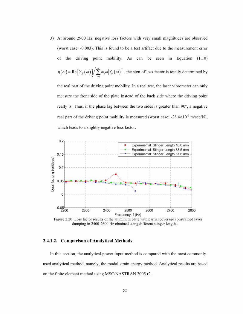
55

3) At around 2900 Hz, negative loss factors with very small magnitudes are observed

(worst case: -0.003). This is found to be a test artifact due to the measurement error

of the driving point mobility. As can be seen in Equation (1.10)

( ) ( ) ( )2

1

ReN

ff i if

i

Y m Yη ω ω ω ω=

= ∑ , the sign of loss factor is totally determined by

the real part of the driving point mobility. In a real test, the laser vibrometer can only

measure the front side of the plate instead of the back side where the driving point

really is. Thus, if the phase lag between the two sides is greater than 90°, a negative

real part of the driving point mobility is measured (worst case: -28.4×10-6

m/sec/N),

which leads to a slightly negative loss factor.

2200 2300 2400 2500 2600 2700 2800-0.05

0

0.05

0.1

0.15

0.2

Frequency, f (Hz)

Loss facto

r η (unitle

ss)

Experimental: Stinger Length 18.0 mm



Figure 2.20 Loss factor results of the aluminum plate with partial coverage constrained layer

damping in 2400-2600 Hz obtained using different stinger lengths.

2.4.1.2. Comparison of Analytical Methods

In this section, the analytical power input method is compared with the most commonly-

used analytical method, namely, the modal strain energy method. Analytical results are based

on the finite element method using MSC/NASTRAN 2005 r2.

56

The analytical power input method is used to estimate loss factors from the direct

frequency response solution (MSC/NASTRAN solution 108). Frequency Response Functions

(FRFs) of the driving point and the strain energy of the whole structure at each frequency are

extracted. Since this is a non-uniformly damped structure, the ith portion’s mass im is not

constant over the plate.

For the purpose of comparison, the modal strain energy method is used to estimate loss

factors using the normal mode solution (MSC/NASTRAN solution 103). Strain energy ratios

are extracted. It is noted that the modal strain energy method tends to overestimate loss

factors [83] [84]. The error increases with the loss factor of the viscoelastic material VEM

η and

goes to zero as 2 1

0G G → [84]:

( ) 2 2

2 3 32 2 2 2

1 2 1 1 2 1

1r

VEM

G GG G G G

G G G G G G

η η ηη

η η

∆ − = = + + +

(2.48)

In this research, this error is estimated by the material properties of the viscoelastic material

at 5000 Hz: 0.9VEM

η = , 6

29 10G = × Pa and the material properties of the aluminum:

10

1 37.45 10G G= = × Pa. The error ( 82.36 10−× ) turns out to be harmless to the loss factor

results in this research.

Loss factor results are shown in Figure 2.21. The two analytical methods yield results

which show modestly good agreement once one considers several reasons to discount some

features of the two results. First, at certain frequencies (e.g., 2118 Hz and 2913 Hz), the

modal strain energy method yields “abnormally” high or low loss factors estimations. A

closer look into the corresponding mode shapes reveals the reason. As shown in Figure

2.22(a), at 2118 Hz, the mode shape involves large displacement in the central damped

region. So as a result, the ratio of strain energy stored in the viscoelastic material to the strain

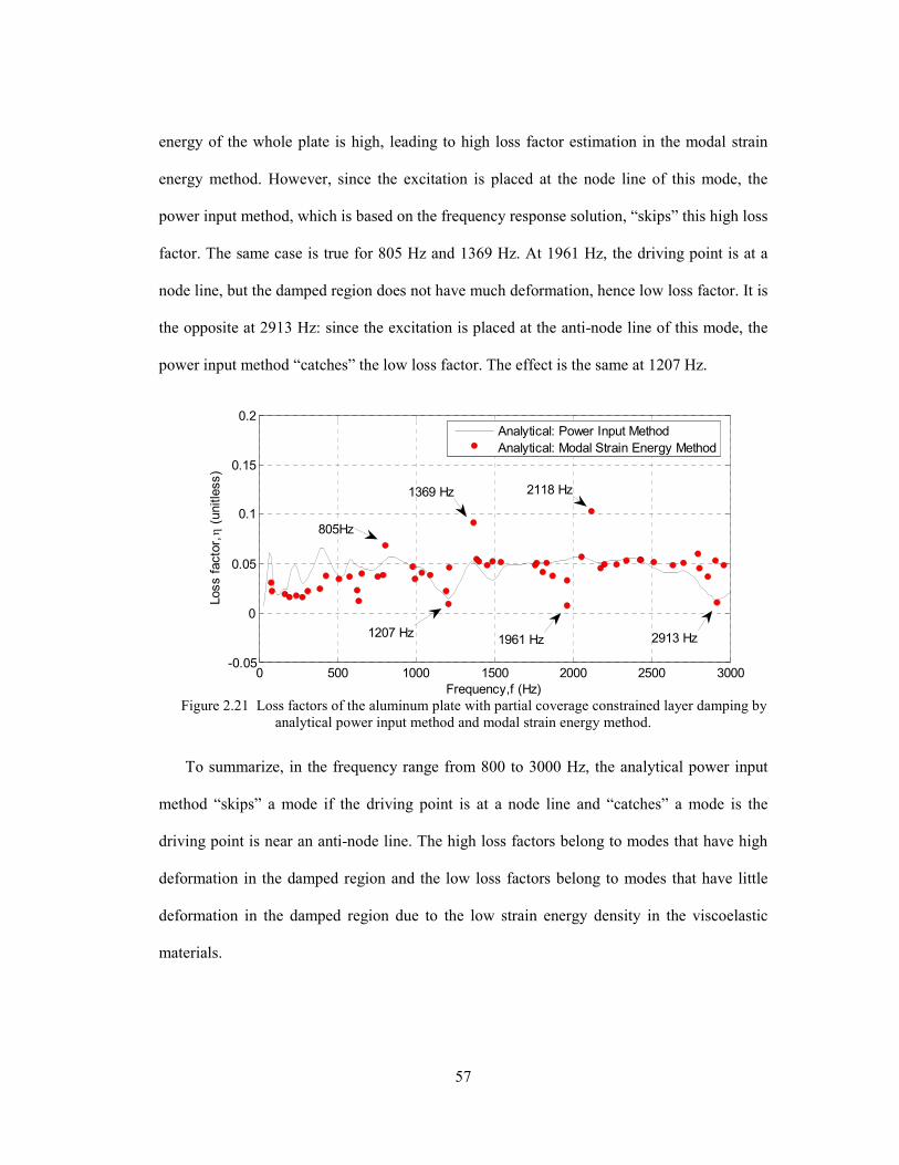
57

energy of the whole plate is high, leading to high loss factor estimation in the modal strain

energy method. However, since the excitation is placed at the node line of this mode, the

power input method, which is based on the frequency response solution, “skips” this high loss

factor. The same case is true for 805 Hz and 1369 Hz. At 1961 Hz, the driving point is at a

node line, but the damped region does not have much deformation, hence low loss factor. It is

the opposite at 2913 Hz: since the excitation is placed at the anti-node line of this mode, the

power input method “catches” the low loss factor. The effect is the same at 1207 Hz.

0 500 1000 1500 2000 2500 3000-0.05

0

0.05

0.1

0.15

0.2

Loss facto

r, η

(unitle

ss)

Frequency,f (Hz)

Analytical: Power Input Method

Analytical: Modal Strain Energy Method

2118 Hz1369 Hz

1207 Hz

805Hz

1961 Hz 2913 Hz

Figure 2.21 Loss factors of the aluminum plate with partial coverage constrained layer damping by

analytical power input method and modal strain energy method.

To summarize, in the frequency range from 800 to 3000 Hz, the analytical power input

method “skips” a mode if the driving point is at a node line and “catches” a mode is the

driving point is near an anti-node line. The high loss factors belong to modes that have high

deformation in the damped region and the low loss factors belong to modes that have little

deformation in the damped region due to the low strain energy density in the viscoelastic

materials.

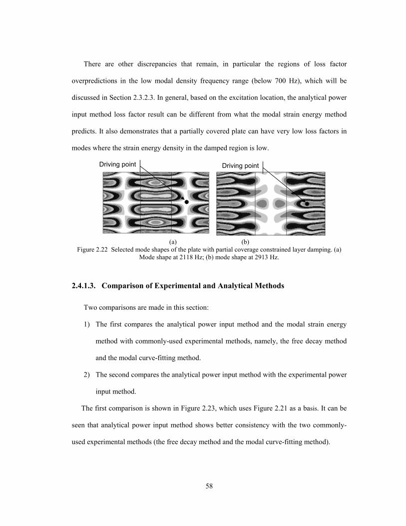
58

There are other discrepancies that remain, in particular the regions of loss factor

overpredictions in the low modal density frequency range (below 700 Hz), which will be

discussed in Section 2.3.2.3. In general, based on the excitation location, the analytical power

input method loss factor result can be different from what the modal strain energy method

predicts. It also demonstrates that a partially covered plate can have very low loss factors in

modes where the strain energy density in the damped region is low.

(a) (b)

Figure 2.22 Selected mode shapes of the plate with partial coverage constrained layer damping. (a)

Mode shape at 2118 Hz; (b) mode shape at 2913 Hz.

2.4.1.3. Comparison of Experimental and Analytical Methods

Two comparisons are made in this section:

1) The first compares the analytical power input method and the modal strain energy

method with commonly-used experimental methods, namely, the free decay method

and the modal curve-fitting method.

2) The second compares the analytical power input method with the experimental power

input method.

The first comparison is shown in Figure 2.23, which uses Figure 2.21 as a basis. It can be

seen that analytical power input method shows better consistency with the two commonly-

used experimental methods (the free decay method and the modal curve-fitting method).

Driving pointDriving point

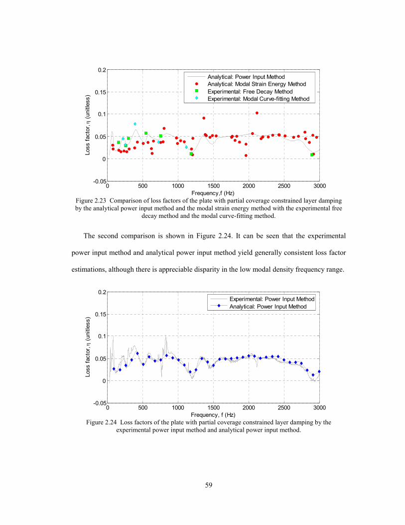
59

0 500 1000 1500 2000 2500 3000-0.05

0

0.05

0.1

0.15

0.2

Loss facto

r, η

(unitle

ss)

Frequency,f (Hz)




Experimental: Modal Curve-fitting Method

Figure 2.23 Comparison of loss factors of the plate with partial coverage constrained layer damping

by the analytical power input method and the modal strain energy method with the experimental free

decay method and the modal curve-fitting method.

The second comparison is shown in Figure 2.24. It can be seen that the experimental

power input method and analytical power input method yield generally consistent loss factor

estimations, although there is appreciable disparity in the low modal density frequency range.

0 500 1000 1500 2000 2500 3000-0.05

0

0.05

0.1

0.15

0.2

Loss facto

r, η

(unitle

ss)

Frequency, f (Hz)



Figure 2.24 Loss factors of the plate with partial coverage constrained layer damping by the

experimental power input method and analytical power input method.

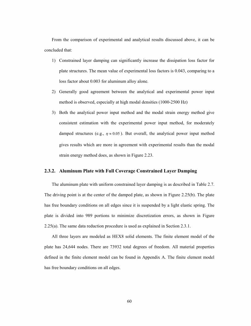
60

From the comparison of experimental and analytical results discussed above, it can be

concluded that:

1) Constrained layer damping can significantly increase the dissipation loss factor for

plate structures. The mean value of experimental loss factors is 0.043, comparing to a

loss factor about 0.003 for aluminum alloy alone.

2) Generally good agreement between the analytical and experimental power input

method is observed, especially at high modal densities (1000-2500 Hz)

3) Both the analytical power input method and the modal strain energy method give

consistent estimation with the experimental power input method, for moderately

damped structures (e.g., 05.0≈η ). But overall, the analytical power input method

gives results which are more in agreement with experimental results than the modal

strain energy method does, as shown in Figure 2.23.

2.3.2. Aluminum Plate with Full Coverage Constrained Layer Damping

The aluminum plate with uniform constrained layer damping is as described in Table 2.7.

The driving point is at the center of the damped plate, as shown in Figure 2.25(b). The plate

has free boundary conditions on all edges since it is suspended by a light elastic spring. The

plate is divided into 989 portions to minimize discretization errors, as shown in Figure

2.25(a). The same data reduction procedure is used as explained in Section 2.3.1.

All three layers are modeled as HEX8 solid elements. The finite element model of the

plate has 24,644 nodes. There are 73932 total degrees of freedom. All material properties

defined in the finite element model can be found in Appendix A. The finite element model

has free boundary conditions on all edges.

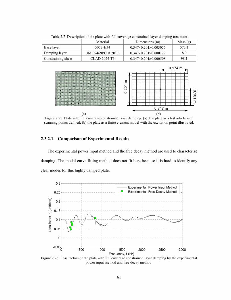
61

Table 2.7 Description of the plate with full coverage constrained layer damping treatment


Base layer 5052-H34 0.347×0.201×0.003055 572.1

Damping layer 3M F9469PC at 20°C 0.347×0.201×0.000127 8.9

Constraining sheet CLAD 2024-T3 0.347×0.201×0.000508 98.1

(a) (b)

Figure 2.25 Plate with full coverage constrained layer damping. (a) The plate as a test article with

scanning points defined; (b) the plate as a finite element model with the excitation point illustrated.

2.3.2.1. Comparison of Experimental Results

The experimental power input method and the free decay method are used to characterize

damping. The modal curve-fitting method does not fit here because it is hard to identify any

clear modes for this highly damped plate.

0 500 1000 1500 2000 2500 3000-0.05

0

0.05

0.1

0.15

0.2

0.25

0.3

Loss facto

r, η

(unitle

ss)

Frequency, f (Hz)



Figure 2.26 Loss factors of the plate with full coverage constrained layer damping by the experimental

power input method and free decay method.

0.1

01 m

0.2

01 m

0.347 m

0.174 m

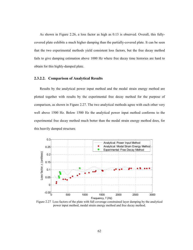
62

As shown in Figure 2.26, a loss factor as high as 0.13 is observed. Overall, this fully-

covered plate exhibits a much higher damping than the partially-covered plate. It can be seen

that the two experimental methods yield consistent loss factors, but the free decay method

fails to give damping estimation above 1000 Hz where free decay time histories are hard to

obtain for this highly-damped plate.

2.3.2.2. Comparison of Analytical Results

Results by the analytical power input method and the modal strain energy method are

plotted together with results by the experimental free decay method for the purpose of

comparison, as shown in Figure 2.27. The two analytical methods agree with each other very

well above 1500 Hz. Below 1500 Hz the analytical power input method conforms to the

experimental free decay method much better than the modal strain energy method does, for

this heavily damped structure.

0 500 1000 1500 2000 2500 3000-0.05

0

0.05

0.1

0.15

0.2

0.25

0.3

Loss facto

r, η

(unitle

ss)

Frequency, f (Hz)




Figure 2.27 Loss factors of the plate with full coverage constrained layer damping by the analytical

power input method, modal strain energy method and free decay method.

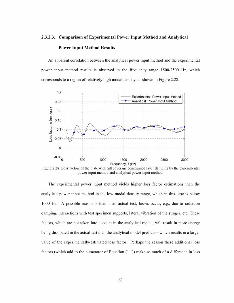
63

2.3.2.3. Comparison of Experimental Power Input Method and Analytical

Power Input Method Results

An apparent correlation between the analytical power input method and the experimental

power input method results is observed in the frequency range 1500-2500 Hz, which

corresponds to a region of relatively high modal density, as shown in Figure 2.28.

0 500 1000 1500 2000 2500 3000-0.05

0

0.05

0.1

0.15

0.2

0.25

0.3

Loss facto

r, η

(unitle

ss)

Frequency, f (Hz)



Figure 2.28 Loss factors of the plate with full coverage constrained layer damping by the experimental

power input method and analytical power input method.

The experimental power input method yields higher loss factor estimations than the

analytical power input method in the low modal density range, which in this case is below

1000 Hz. A possible reason is that in an actual test, losses occur, e.g., due to radiation

damping, interactions with test specimen supports, lateral vibration of the stinger, etc. These

factors, which are not taken into account in the analytical model, will result in more energy

being dissipated in the actual test than the analytical model predicts—which results in a larger

value of the experimentally-estimated loss factor. Perhaps the reason these additional loss

factors (which add to the numerator of Equation (1.1)) make so much of a difference in loss

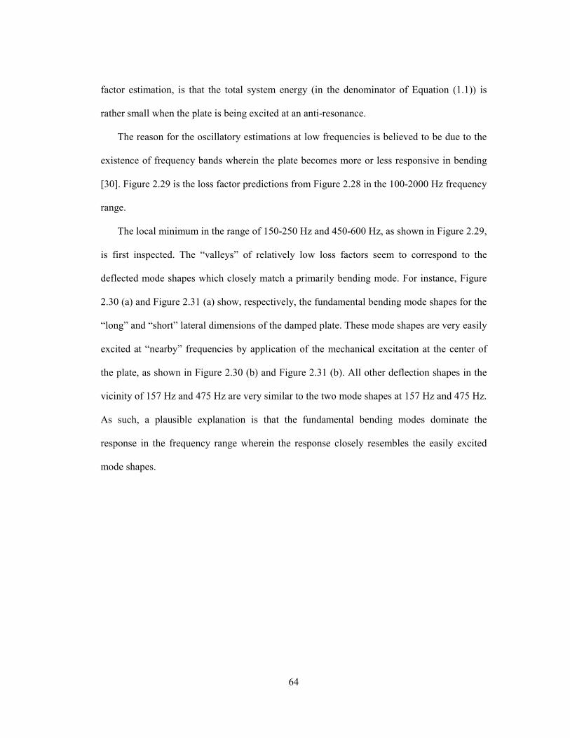
64

factor estimation, is that the total system energy (in the denominator of Equation (1.1)) is

rather small when the plate is being excited at an anti-resonance.

The reason for the oscillatory estimations at low frequencies is believed to be due to the

existence of frequency bands wherein the plate becomes more or less responsive in bending

[30]. Figure 2.29 is the loss factor predictions from Figure 2.28 in the 100-2000 Hz frequency

range.

The local minimum in the range of 150-250 Hz and 450-600 Hz, as shown in Figure 2.29,

is first inspected. The “valleys” of relatively low loss factors seem to correspond to the

deflected mode shapes which closely match a primarily bending mode. For instance, Figure

2.30 (a) and Figure 2.31 (a) show, respectively, the fundamental bending mode shapes for the

“long” and “short” lateral dimensions of the damped plate. These mode shapes are very easily

excited at “nearby” frequencies by application of the mechanical excitation at the center of

the plate, as shown in Figure 2.30 (b) and Figure 2.31 (b). All other deflection shapes in the

vicinity of 157 Hz and 475 Hz are very similar to the two mode shapes at 157 Hz and 475 Hz.

As such, a plausible explanation is that the fundamental bending modes dominate the

response in the frequency range wherein the response closely resembles the easily excited

mode shapes.

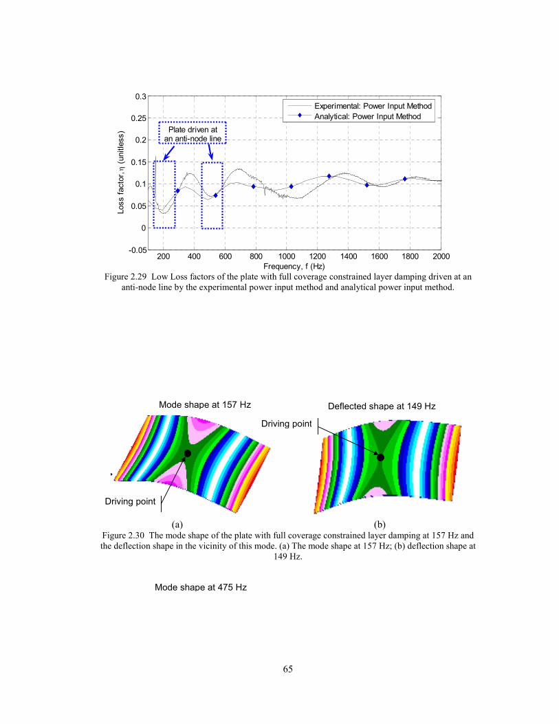
65

200 400 600 800 1000 1200 1400 1600 1800 2000-0.05

0

0.05

0.1

0.15

0.2

0.25

0.3

Loss facto

r, η

(unitle

ss)

Frequency, f (Hz)



Plate driven atan anti-node line

Figure 2.29 Low Loss factors of the plate with full coverage constrained layer damping driven at an

anti-node line by the experimental power input method and analytical power input method.

(a) (b) Figure 2.30 The mode shape of the plate with full coverage constrained layer damping at 157 Hz and

the deflection shape in the vicinity of this mode. (a) The mode shape at 157 Hz; (b) deflection shape at

149 Hz.

Mode shape at 157 Hz Deflected shape at 149 Hz

Mode shape at 475 Hz

Driving point

Driving point

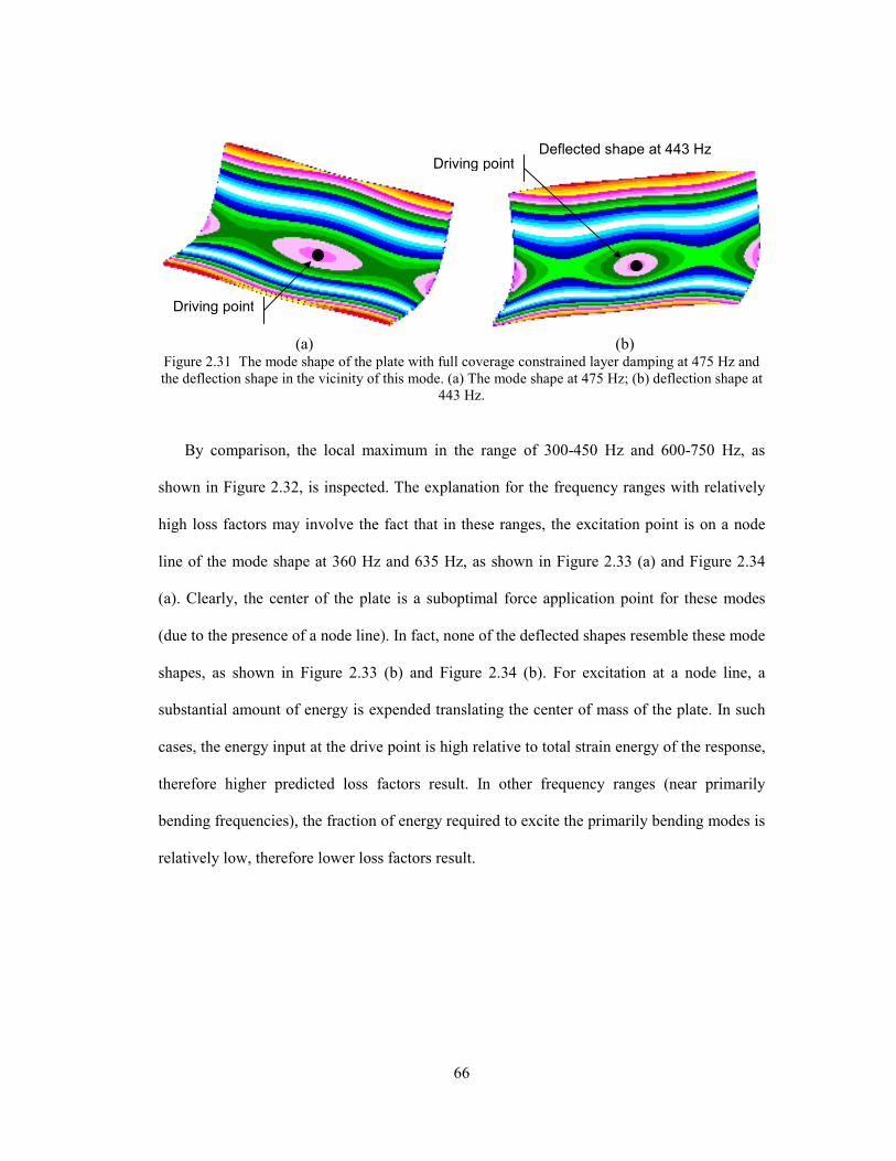
66



443 Hz.

By comparison, the local maximum in the range of 300-450 Hz and 600-750 Hz, as

shown in Figure 2.32, is inspected. The explanation for the frequency ranges with relatively

high loss factors may involve the fact that in these ranges, the excitation point is on a node

line of the mode shape at 360 Hz and 635 Hz, as shown in Figure 2.33 (a) and Figure 2.34

(a). Clearly, the center of the plate is a suboptimal force application point for these modes

(due to the presence of a node line). In fact, none of the deflected shapes resemble these mode

shapes, as shown in Figure 2.33 (b) and Figure 2.34 (b). For excitation at a node line, a

substantial amount of energy is expended translating the center of mass of the plate. In such

cases, the energy input at the drive point is high relative to total strain energy of the response,

therefore higher predicted loss factors result. In other frequency ranges (near primarily

bending frequencies), the fraction of energy required to excite the primarily bending modes is

relatively low, therefore lower loss factors result.

Deflected shape at 443 Hz

Driving point

Driving point

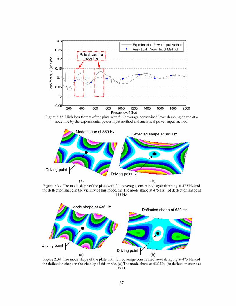
67

200 400 600 800 1000 1200 1400 1600 1800 2000-0.05

0

0.05

0.1

0.15

0.2

0.25

0.3

Loss facto

r, η

(unitle

ss)

Frequency, f (Hz)



Plate driven at anode line

Figure 2.32 High loss factors of the plate with full coverage constrained layer damping driven at a

node line by the experimental power input method and analytical power input method.



443 Hz.



639 Hz.



Driving point

Driving point

Driving pointDriving point

68

2.3.3. Composite Honeycomb Sandwich Beam with Aluminum Stand-Off

Constrained Layer Damping

Carbon-fiber reinforced plastic composite structures usually possess high specific

stiffness. The bending stiffness will be further increased by adding a honeycomb layer in

between carbon facesheets, which is common for aircraft fuselage and bulkhead structures. In

contrary to riveted metal structures, composite honeycomb sandwich structures have low

intrinsic damping, due to lack of friction between structural components. So added damping

becomes necessary for noise reduction.

In this research, aluminum alloy 2024-T3 is first chosen as the stand-off material,

considering stiffness, material availability, etc. The manufactured stand-offs are in 1 cm×1

cm squares, 1 mm apart. The 1 mm groves are cut to reduce the bending stiffness of the

aluminum stand-offs. The stand-offs are bonded to carbon facesheets by epoxy under vacuum

pressure, then a damping layer and a constraining layer are added, as shown in Figure 2.35

and Table 2.8. The beam has free boundary conditions on all edges as it is suspended by two

light elastic springs.

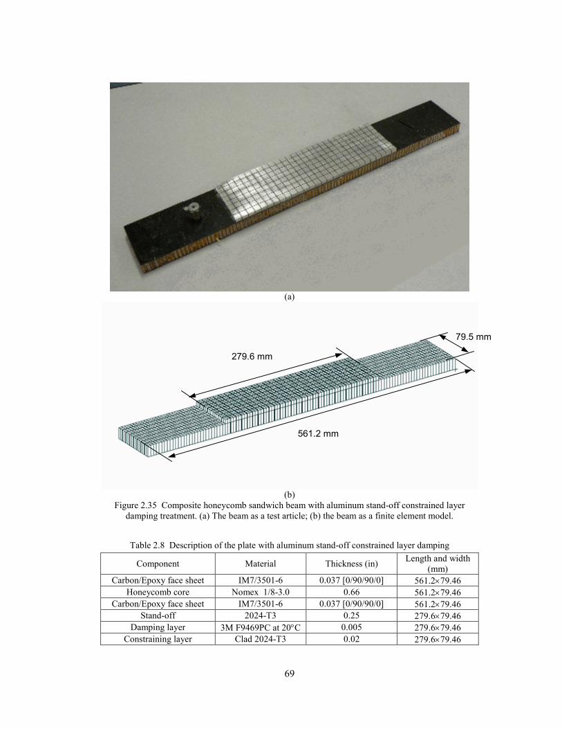
69

(a)

(b)

Figure 2.35 Composite honeycomb sandwich beam with aluminum stand-off constrained layer

damping treatment. (a) The beam as a test article; (b) the beam as a finite element model.

Table 2.8 Description of the plate with aluminum stand-off constrained layer damping

Component Material Thickness (in) Length and width

(mm)

Carbon/Epoxy face sheet IM7/3501-6 0.037 [0/90/90/0] 561.2×79.46

Honeycomb core Nomex 1/8-3.0 0.66 561.2×79.46


Stand-off 2024-T3 0.25 279.6×79.46

Damping layer 3M F9469PC at 20°C 0.005 279.6×79.46

Constraining layer Clad 2024-T3 0.02 279.6×79.46

279.6 mm

561.2 mm

79.5 mm

70

The finite element model of the plate has 17236 nodes. The total degrees of freedom are

79298. The two composite facesheets and the constraining layer are modeled as QUAD4

elements. The honeycomb, stand-offs and the viscoelastic layer are modeled as HEX8 solid

elements. All material properties defined in the finite element model can be found in

Appendix A. The finite element model has free boundary conditions on all edges.

Experimental and analytical power input method results are shown in Figure 2.36.

Conclusions include:

1) Stand-off constrained layer damping yields a significantly higher damping level

than generic constrained layer damping, with less damping material (222 cm2 for

SOCLD beam vs. 697 cm2

for fully covered monolithic CLD plate vs. 207 cm2

for partially covered monolithic CLD plate).

2) The same correlation as shown in Section 2.3.2.3 is observed in between the two

results. The modeling issues related to the frequency mismatch between the local

loss factor maxima and minima seem to be the same.

3) The discrepancy between experimental and analytical results may be due to lack

of accurate material property information on carbon fiber composites and

honeycomb core. Also the aluminum stand-off on the test article is more massive

than in the model because a thin layer of aluminum is left to act as linkage

between neighboring stand-off units. This will make the actual stand-off more

stiff, which is consistent with the results in Figure 2.36.

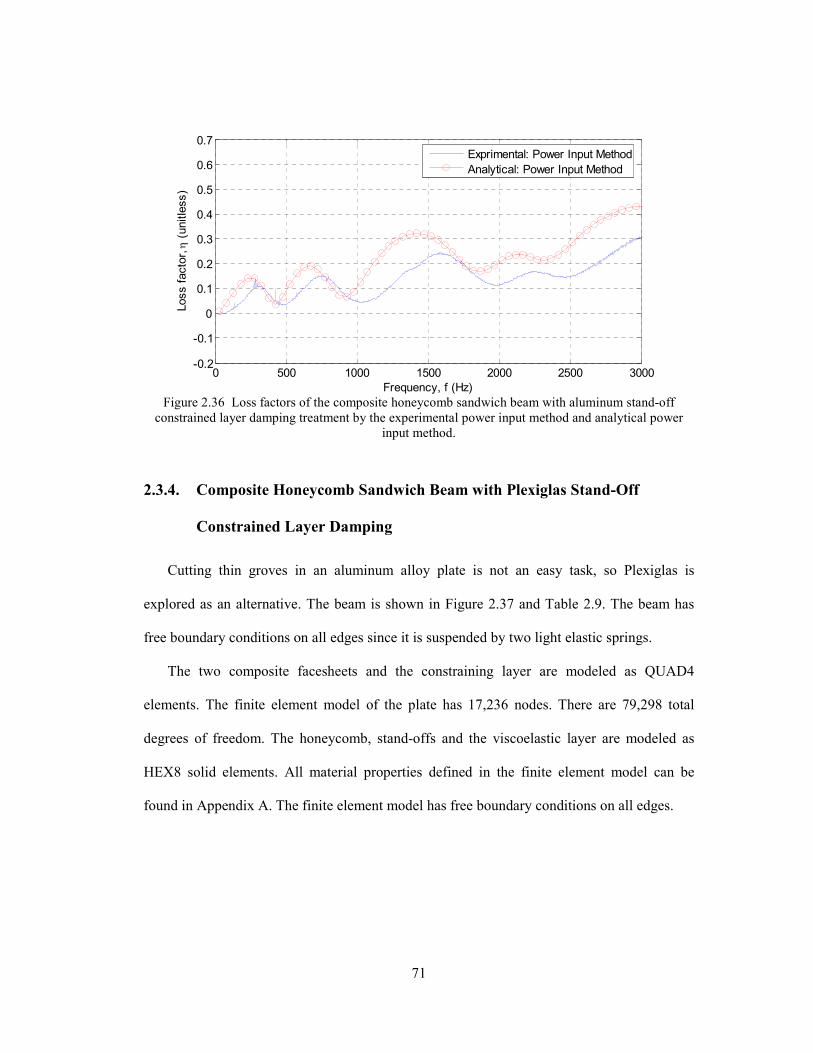
71

0 500 1000 1500 2000 2500 3000-0.2

-0.1

0

0.1

0.2

0.3

0.4

0.5

0.6

0.7

Loss facto

r, η

(unitle

ss)

Frequency, f (Hz)

Exprimental: Power Input Method


Figure 2.36 Loss factors of the composite honeycomb sandwich beam with aluminum stand-off

constrained layer damping treatment by the experimental power input method and analytical power

input method.

2.3.4. Composite Honeycomb Sandwich Beam with Plexiglas Stand-Off

Constrained Layer Damping

Cutting thin groves in an aluminum alloy plate is not an easy task, so Plexiglas is

explored as an alternative. The beam is shown in Figure 2.37 and Table 2.9. The beam has

free boundary conditions on all edges since it is suspended by two light elastic springs.

The two composite facesheets and the constraining layer are modeled as QUAD4

elements. The finite element model of the plate has 17,236 nodes. There are 79,298 total

degrees of freedom. The honeycomb, stand-offs and the viscoelastic layer are modeled as

HEX8 solid elements. All material properties defined in the finite element model can be

found in Appendix A. The finite element model has free boundary conditions on all edges.

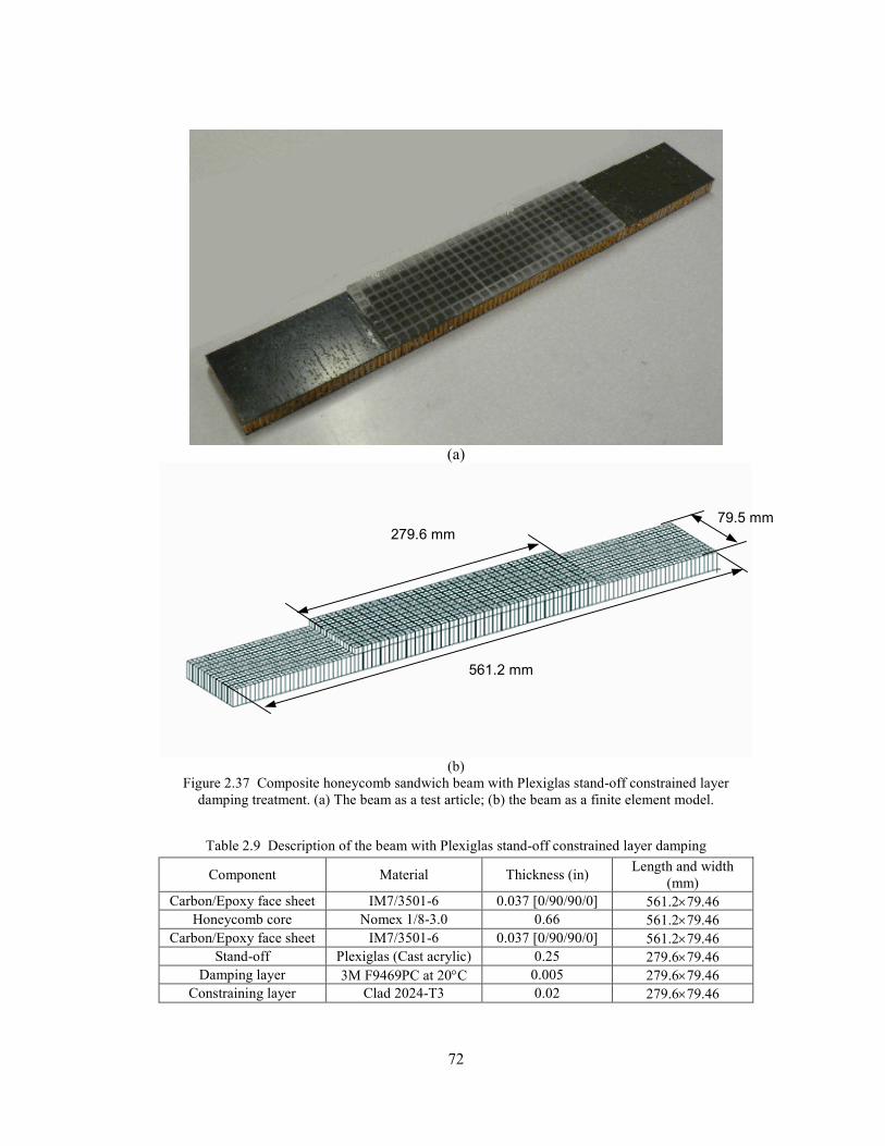
72

(a)

(b)

Figure 2.37 Composite honeycomb sandwich beam with Plexiglas stand-off constrained layer

damping treatment. (a) The beam as a test article; (b) the beam as a finite element model.

Table 2.9 Description of the beam with Plexiglas stand-off constrained layer damping

Component Material Thickness (in) Length and width

(mm)


Honeycomb core Nomex 1/8-3.0 0.66 561.2×79.46


Stand-off Plexiglas (Cast acrylic) 0.25 279.6×79.46

Damping layer 3M F9469PC at 20°C 0.005 279.6×79.46

Constraining layer Clad 2024-T3 0.02 279.6×79.46

561.2 mm

79.5 mm 279.6 mm

73

Experimental and analytical power input method results are shown in Figure 2.38.

Conclusions include:

1) Stand-offs made of Plexiglas yield a lower damping level than stand-offs made of

aluminum, which is due to the stiffness difference. The overall damping level of

Plexiglas stand-offs is still significantly higher than that of generic constrained

layer damping.

2) Issues of correlation between the experimental power input method and the

analytical power input method noted in Section 2.3.3 are observed, but to a

slightly lower degree.

3) Discrepancy between experimental and analytical results may be due to lack of

accurate material property information on carbon fiber composites and

honeycomb core.

0 500 1000 1500 2000 2500 3000-0.2

-0.1

0

0.1

0.2

0.3

0.4

0.5

0.6

0.7

Loss facto

r, η

(unitle

ss)

Frequency, f (Hz)

Exprimental: Power Input Method


Figure 2.38 Loss factors of the composite honeycomb sandwich beam with Plexiglas stand-off

constrained layer damping by the experimental power input method and the analytical power input

method.

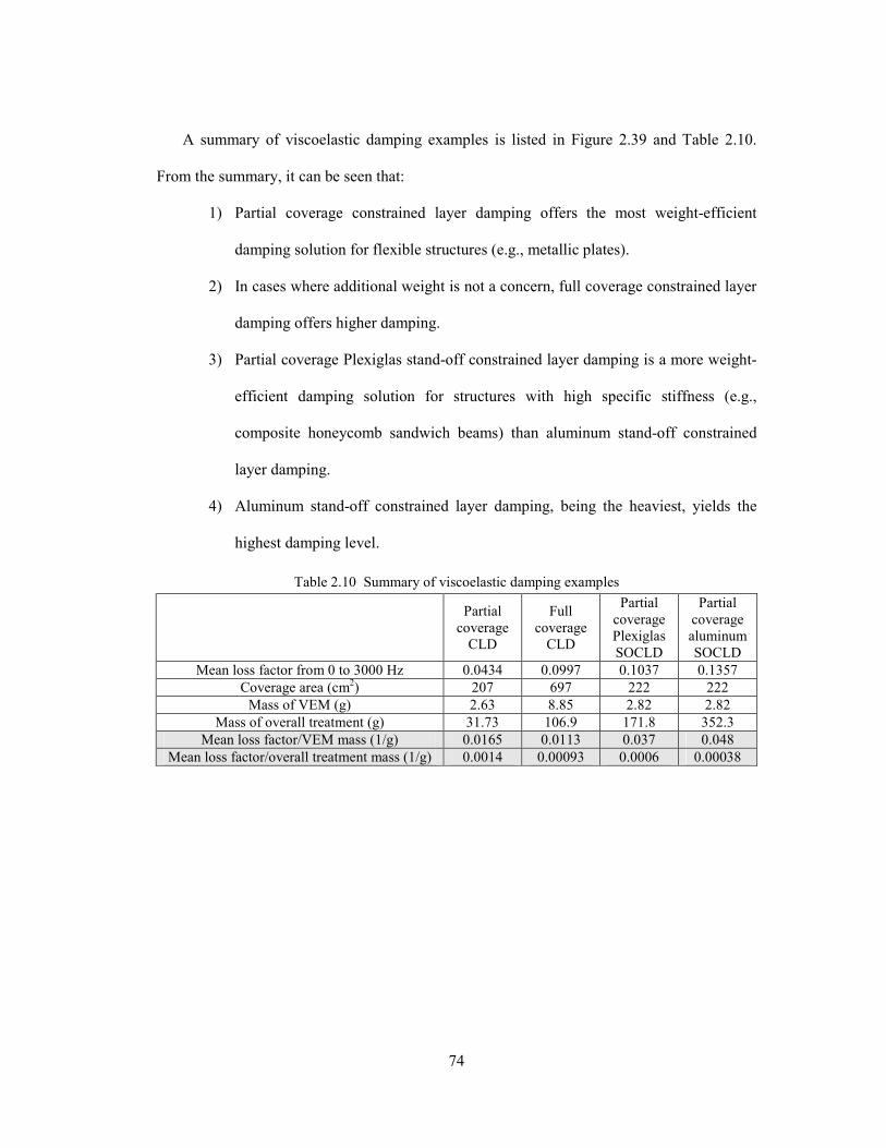
74

A summary of viscoelastic damping examples is listed in Figure 2.39 and Table 2.10.

From the summary, it can be seen that:

1) Partial coverage constrained layer damping offers the most weight-efficient

damping solution for flexible structures (e.g., metallic plates).

2) In cases where additional weight is not a concern, full coverage constrained layer

damping offers higher damping.

3) Partial coverage Plexiglas stand-off constrained layer damping is a more weight-

efficient damping solution for structures with high specific stiffness (e.g.,

composite honeycomb sandwich beams) than aluminum stand-off constrained

layer damping.

4) Aluminum stand-off constrained layer damping, being the heaviest, yields the

highest damping level.

Table 2.10 Summary of viscoelastic damping examples

Partial

coverage

CLD

Full

coverage

CLD

Partial

coverage

Plexiglas

SOCLD

Partial

coverage

aluminum

SOCLD

Mean loss factor from 0 to 3000 Hz 0.0434 0.0997 0.1037 0.1357

Coverage area (cm2) 207 697 222 222

Mass of VEM (g) 2.63 8.85 2.82 2.82

Mass of overall treatment (g) 31.73 106.9 171.8 352.3

Mean loss factor/VEM mass (1/g) 0.0165 0.0113 0.037 0.048

Mean loss factor/overall treatment mass (1/g) 0.0014 0.00093 0.0006 0.00038

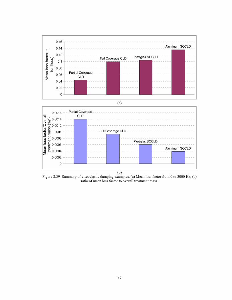
75

Partial Coverage

CLD

Full Coverage CLD Plexiglas SOCLD

Aluminum SOCLD

0

0.02

0.04

0.06

0.08

0.1

0.12

0.14

0.16

(a)

Aluminum SOCLD

Plexiglas SOCLD

Full Coverage CLD

Partial Coverage

CLD

0

0.0002

0.0004

0.0006

0.0008

0.001

0.0012

0.0014

0.0016

(b)

Figure 2.39 Summary of viscoelastic damping examples. (a) Mean loss factor from 0 to 3000 Hz; (b)

ratio of mean loss factor to overall treatment mass.

Mean loss facto

r, η

(unitle

ss)

Mean loss facto

r/O

vera

ll

treatm

ent m

ass (1/g

)

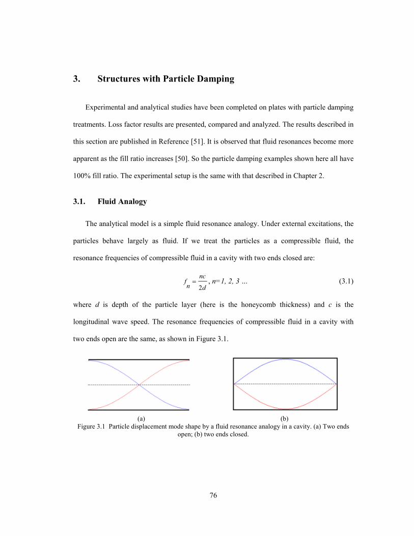
76

3. Structures with Particle Damping

Experimental and analytical studies have been completed on plates with particle damping

treatments. Loss factor results are presented, compared and analyzed. The results described in

this section are published in Reference [51]. It is observed that fluid resonances become more

apparent as the fill ratio increases [50]. So the particle damping examples shown here all have

100% fill ratio. The experimental setup is the same with that described in Chapter 2.

3.1. Fluid Analogy

The analytical model is a simple fluid resonance analogy. Under external excitations, the

particles behave largely as fluid. If we treat the particles as a compressible fluid, the

resonance frequencies of compressible fluid in a cavity with two ends closed are:

d

nc

nf

2= , n=1, 2, 3 … (3.1)

where d is depth of the particle layer (here is the honeycomb thickness) and c is the

longitudinal wave speed. The resonance frequencies of compressible fluid in a cavity with

two ends open are the same, as shown in Figure 3.1.

(a) (b)

Figure 3.1 Particle displacement mode shape by a fluid resonance analogy in a cavity. (a) Two ends

open; (b) two ends closed.

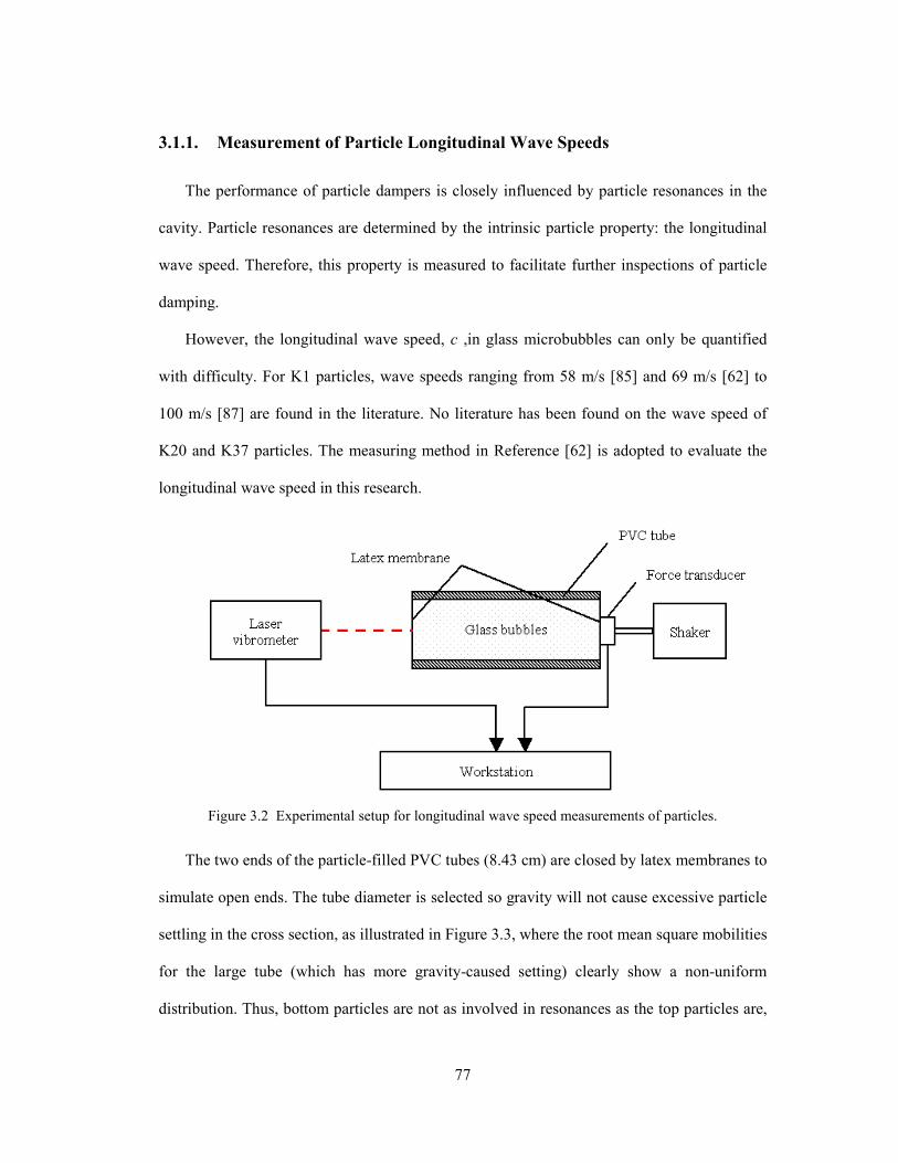
77

3.1.1. Measurement of Particle Longitudinal Wave Speeds

The performance of particle dampers is closely influenced by particle resonances in the

cavity. Particle resonances are determined by the intrinsic particle property: the longitudinal

wave speed. Therefore, this property is measured to facilitate further inspections of particle

damping.

However, the longitudinal wave speed, c ,in glass microbubbles can only be quantified

with difficulty. For K1 particles, wave speeds ranging from 58 m/s [85] and 69 m/s [62] to

100 m/s [87] are found in the literature. No literature has been found on the wave speed of

K20 and K37 particles. The measuring method in Reference [62] is adopted to evaluate the

longitudinal wave speed in this research.

Figure 3.2 Experimental setup for longitudinal wave speed measurements of particles.

The two ends of the particle-filled PVC tubes (8.43 cm) are closed by latex membranes to

simulate open ends. The tube diameter is selected so gravity will not cause excessive particle

settling in the cross section, as illustrated in Figure 3.3, where the root mean square mobilities

for the large tube (which has more gravity-caused setting) clearly show a non-uniform

distribution. Thus, bottom particles are not as involved in resonances as the top particles are,

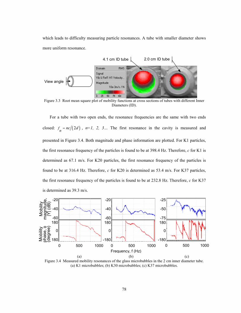
78

which leads to difficulty measuring particle resonances. A tube with smaller diameter shows

more uniform resonance.

Figure 3.3 Root mean square plot of mobility functions at cross sections of tubes with different Inner

Diameters (ID).

For a tube with two open ends, the resonance frequencies are the same with two ends

closed: ( )2fn

nc d= , n=1, 2, 3… The first resonance in the cavity is measured and

presented in Figure 3.4. Both magnitude and phase information are plotted. For K1 particles,

the first resonance frequency of the particles is found to be at 398.4 Hz. Therefore, c for K1 is

determined as 67.1 m/s. For K20 particles, the first resonance frequency of the particles is

found to be at 316.4 Hz. Therefore, c for K20 is determined as 53.4 m/s. For K37 particles,

the first resonance frequency of the particles is found to be at 232.8 Hz. Therefore, c for K37

is determined as 39.3 m/s.

(a) (b) (c)

Figure 3.4 Measured mobility resonances of the glass microbubbles in the 2 cm inner diameter tube.

(a) K1 microbubbles; (b) K30 microbubbles; (c) K37 microbubbles.

-20

-40

-60180

0

-180

View angle

-20

-40

-60180

0

-180

Frequency, f (Hz)

0 500 1000

-25

-50

-75180

0

-180

0 500 1000 0 500 1000

Mobility

m

agnitude,

|Y| (d

B)

Mobility

phase, φ

(degre

e)

4.1 cm ID tube 2.0 cm ID tube

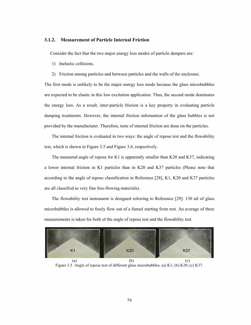
79

3.1.2. Measurement of Particle Internal Friction

Consider the fact that the two major energy loss modes of particle dampers are:

1) Inelastic collisions.

2) Friction among particles and between particles and the walls of the enclosure.

The first mode is unlikely to be the major energy loss mode because the glass microbubbles

are expected to be elastic in this low excitation application. Thus, the second mode dominates

the energy loss. As a result, inter-particle friction is a key property in evaluating particle

damping treatments. However, the internal friction information of the glass bubbles is not

provided by the manufacturer. Therefore, tests of internal friction are done on the particles.

The internal friction is evaluated in two ways: the angle of repose test and the flowability

test, which is shown in Figure 3.5 and Figure 3.6, respectively.

The measured angle of repose for K1 is apparently smaller than K20 and K37, indicating

a lower internal friction in K1 particles than in K20 and K37 particles (Please note that

according to the angle of repose classification in Reference [28], K1, K20 and K37 particles

are all classified as very fine free-flowing materials).

The flowability test instrument is designed referring to Reference [29]: 130 ml of glass

microbubbles is allowed to freely flow out of a funnel starting from rest. An average of three

measurements is taken for both of the angle of repose test and the flowability test.

(a) (b) (c)

Figure 3.5 Angle of repose test of different glass microbubbles. (a) K1; (b) K20; (c) K37.

K1 K20 K37

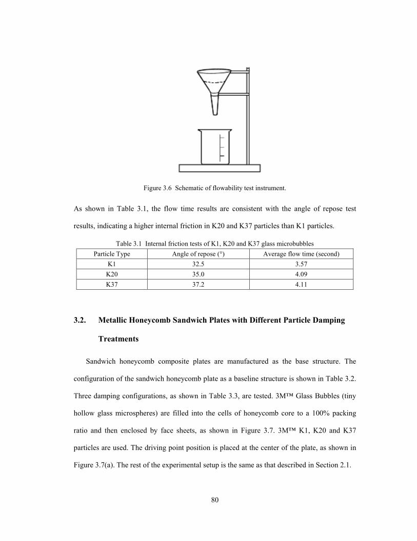
80

Figure 3.6 Schematic of flowability test instrument.

As shown in Table 3.1, the flow time results are consistent with the angle of repose test

results, indicating a higher internal friction in K20 and K37 particles than K1 particles.

Table 3.1 Internal friction tests of K1, K20 and K37 glass microbubbles

Particle Type Angle of repose (°) Average flow time (second)

K1 32.5 3.57

K20 35.0 4.09

K37 37.2 4.11

3.2. Metallic Honeycomb Sandwich Plates with Different Particle Damping

Treatments

Sandwich honeycomb composite plates are manufactured as the base structure. The

configuration of the sandwich honeycomb plate as a baseline structure is shown in Table 3.2.

Three damping configurations, as shown in Table 3.3, are tested. 3M™ Glass Bubbles (tiny

hollow glass microspheres) are filled into the cells of honeycomb core to a 100% packing

ratio and then enclosed by face sheets, as shown in Figure 3.7. 3M™ K1, K20 and K37

particles are used. The driving point position is placed at the center of the plate, as shown in

Figure 3.7(a). The rest of the experimental setup is the same as that described in Section 2.1.

81

(a)

(b)

Figure 3.7 Sandwich honeycomb plates with particle damping. (a): Schematic of damped plates; (b):

the three specimens filled with different particles.

Driving point

8 in

5.4

375 in

4 in

2.7

29 in

Aluminum plate

Honeycomb

Steel plate Base structure

Glass bubbles

Driving point

82

Table 3.2 Description of metallic sandwich honeycomb plates

Component Material Thickness (in) Length and width (in)

Aluminum face sheet Clad 2024-T3 0.032

Honeycomb core Nomex 1/8-3.0 0.66

Steel base sheet AISI 1018 0.0625

5 716 × 8

Table 3.3 Description of K1, K20 and K37 glass microbubbles

Particle Type Particle density [1]

(g/cm3)

Average particle

diameter [1] (µm)

Total mass of the

damped plate (g)

K1 0.125 65 441

K20 0.20 60 456

K37 0.37 45 495

With the properties measured in Section 3.1 in hand, it is convenient to inspect the

damping measurement, as shown in Figure 3.8. It can be observed from the comparison in

Figure 3.8 that:

1) The experimental power input method and modal curve-fitting method give

consistent results, but the power input method offers more damping information other

than just at a small number of frequencies. In particular, the experimental power

input method allows one to identify the distinct frequency bands within which the

damping is substantially higher.

2) Glass microbubbles, when filled into honeycomb cells, can significantly increase

damping for sandwich honeycomb plates in distinct frequency bands. Moreover, the

frequencies at which damping peak values occur follow the same trend as the friction

indices measured in Section 3.1.

a) The K1 specimen loss factor result shows a “hump” with the maximum value of

0.095 near 2000 Hz. By the fluid resonance model described in Section 3.1, since

K1 particles have a measured longitudinal wave speed of 67.1 m/s, the first

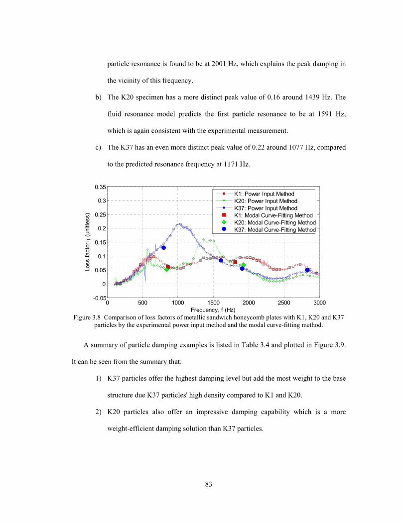
83

particle resonance is found to be at 2001 Hz, which explains the peak damping in

the vicinity of this frequency.

b) The K20 specimen has a more distinct peak value of 0.16 around 1439 Hz. The

fluid resonance model predicts the first particle resonance to be at 1591 Hz,

which is again consistent with the experimental measurement.

c) The K37 has an even more distinct peak value of 0.22 around 1077 Hz, compared

to the predicted resonance frequency at 1171 Hz.

0 500 1000 1500 2000 2500 3000-0.05

0

0.05

0.1

0.15

0.2

0.25

0.3

0.35

Frequency, f (Hz)

Loss facto

r η (unitle

ss)

K1: Power Input Method



K1: Modal Curve-Fitting Method



Figure 3.8 Comparison of loss factors of metallic sandwich honeycomb plates with K1, K20 and K37

particles by the experimental power input method and the modal curve-fitting method.

A summary of particle damping examples is listed in Table 3.4 and plotted in Figure 3.9.

It can be seen from the summary that:

1) K37 particles offer the highest damping level but add the most weight to the base

structure due K37 particles' high density compared to K1 and K20.

2) K20 particles also offer an impressive damping capability which is a more

weight-efficient damping solution than K37 particles.

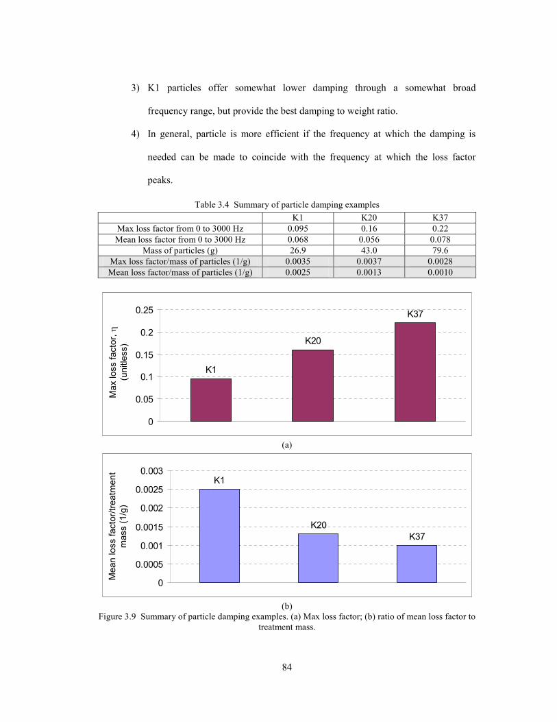
84

3) K1 particles offer somewhat lower damping through a somewhat broad

frequency range, but provide the best damping to weight ratio.

4) In general, particle is more efficient if the frequency at which the damping is

needed can be made to coincide with the frequency at which the loss factor

peaks.

Table 3.4 Summary of particle damping examples

K1 K20 K37

Max loss factor from 0 to 3000 Hz 0.095 0.16 0.22

Mean loss factor from 0 to 3000 Hz 0.068 0.056 0.078

Mass of particles (g) 26.9 43.0 79.6

Max loss factor/mass of particles (1/g) 0.0035 0.0037 0.0028

Mean loss factor/mass of particles (1/g) 0.0025 0.0013 0.0010

K1

K20

K37

0

0.05

0.1

0.15

0.2

0.25

(a)

K37

K20

K1

0

0.0005

0.001

0.0015

0.002

0.0025

0.003

(b)

Figure 3.9 Summary of particle damping examples. (a) Max loss factor; (b) ratio of mean loss factor to

treatment mass.

Max loss facto

r, η

(unitle

ss)

Mean loss facto

r/treatm

ent

mass (1/g

)

85

4. Closure

4.1. Summary

Both experimental and analytical methods of loss factor estimation have been

investigated on two of the most commonly-used passive damping treatments: constrained

layer damping and particle damping.

In summary, the major work in this research includes:

1) Design and manufacture of constrained layer damping, stand-off constrained layer

damping and particle damping treatments for both monolithic and sandwich-

construction beams and plates.

2) Measurement of loss factors for structural panels representative of passenger

enclosures in vehicles using the standard modal curve-fitting method, the free-decay

method and the power input method.

3) Estimation of loss factors for beams and plates with conventional constrained-layer-

damping treatments and stand-off constrained-layer-damping treatments using the

analytical modal strain energy method and the new analytical power input method.

4) Resolution of experimental and analytical methods of damping loss factor estimation

for structural panels with conventional and stand-off constrained layer damping.

5) Measurement of wave speeds in glass microbubbles used as particle dampers.

6) Resolution of frequency bands of high measured damping loss factor for particle

damping in structural panels with the wave speed of particles.

86

4.2. Original Contributions to the Field of Structural Acoustics

1) A new analytical power input method is proposed, validated and applied to

monolithic and sandwich-construction panels with both conventional and stand-off

constrained layer damping configurations. The frequency-dependency of the

viscoelastic materials is directly taken into account in the finite element model used.

This method, then, provides a viable analysis tool for panel constrained layer

damping design.

2) Reasons for the frequency-dependent fluctuation of loss factor estimations

characteristic of the power input methods are explained for the first time in the

literature.

3) Experiments to measure the wave speeds of glass microbubbles in cylindrical

enclosures were conducted.

4) Predicted cavity resonance frequencies, calculated from microbubble wave speeds,

were successfully correlated to frequencies of peak damping loss factor in sandwich

panels with microbubbles particle damping installed in the honeycomb core.

5) Experiments to measure the internal friction of various types of microbubbles were

conducted and correlated in a relative sense with wave speeds and therefore with

frequency of peak damping loss factor.

4.3. Conclusions

1) In frequency ranges where other commonly-used experimental methods apply, the

experimental power input method yields results consistent with the two most

commonly used experimental methods, the free decay method and the modal curve-

fitting method

87

2) In the frequency range associated with high modal density, the analytical power input

method yields results consistent with the (analytical) modal strain energy method and

the experimental power input method.

3) In the low frequency range associated with low modal density, the experimental and

analytical power input methods—with a single point of force/power input—both

predict damping loss factors which oscillate between substantial over-prediction and

near-agreement with the (analytical) modal strain energy method.

a. This effect is a direct result of the point at which the excitation occurs

i. If the excitation point is at a node line for the mode shapes and

deflection response shapes in a broad frequency range, these

methods will overpredict the damping loss factor.

ii. If the excitation point is at an anti-node for the mode shapes and

deflection response shapes in a broad frequency range, these

methods will more accurately predict the damping loss factor.

b. The analytical power input method predicts a slightly higher loss factor

than the modal strain energy method at the frequencies at which the

analytical power input method results are at a local minimum. It is

expected that if a different excitation point is used, the analytical power

input method would have different local minimums. This suggests one

can estimate the damping loss factor in the low modal density range by

"constructing" a curve through the local minimums of the loss factor

curve determined by testing.

4) In the low modal density frequency ranges where both the experimental and

analytical power input methods over-predict loss factor:

88

a. For monolithic plates with conventional constrained layer damping,

i. The experimental power input method predicts even higher loss

factors than the analytical power input method.

ii. The frequencies at which the overpredictions occur tend to agree

between the experimental and analytical methods.

b. For sandwich plates

i. The analytical power input method predicts even higher loss

factors than the experimental method.

ii. The frequencies at which the overpredictions occur are always

lower for the analytical model, suggesting the modeling process

for sandwich plates and/or stand-off damping treatments

underpredicts the structural stiffness of the panel and indicates

needed improvement.

5) The fluid resonance model can predict at which frequency the peak damping

performance will be for particle dampers made of glass microbubbles. This can be

used to tune particle dampers to function at a specific frequency, which leads to the

possibility of suppressing noise/vibration in a specified narrow frequency range (e.g.,

take-off fan blade passage frequency).

6) Results show that the internal friction indices can predict the relative relationship

between peak damping values. It can be used as a particle selection index.

89

4.4. Notes on Applying the Analytical Power Input Method

1) Discretization in the finite element model should be fine enough to capture the

feature size of the frequency response deflection so that there are at least 6-8

elements for a half sine wave.

2) Results show that the displacement in the viscoelastic layer of constraint layer

damping is not strictly linear. So, more than one solid element should be used for the

viscoelastic layer if the computational resource allows.

4.5. Notes on Applying the Experimental Power Input Method

3) The test article should have the velocity measured at points with a spacing that is

capable of capturing the smallest vibration “feature” desired. This can be achieved

by using an analytical model to determine the wavelength of the smallest feature of

the mode shapes for the highest frequency under study. Then, there should be no less

than 2 measurement points over the span of the smallest feature.

4) The shaker armature and stinger should not have a mass over 1/3, but ideally more

like 1/10 of the mass of the test article.

5) The shaker, armature and stinger should have a higher resonance frequency than the

highest frequency of interest.

6) Very long or short stinger lengths should be avoided:

a. Not so long that the stinger vibrates laterally.

b. Not so short that the shaker and test article respond in “pendulum

modes” (both lateral and torsional)

90

4.6. Recommendations for Future Work

1) For either the analytical or experimental power input method, the estimated

damping loss factors are dependent on the excitation position at which a

mechanical shaker is used as excitation source. Therefore, implementing multiple

excitation positions are desirable. In other estimation methods, for example, the

Impulse Response Decay Method (IRDM), multiple hammer excitation positions

are used to obtain a more accurate damping estimation for those structures.

Implementing multiple driving point positions would be very simple in the

analytical power input method, and is feasible for the experimental method.

2) A method to use acoustic excitation would be a great improvement to the

experimental power input method and the analytical power input method to expand

their applicability, especially to structures more complex than a flat structural

panel.

3) A laser vibrometer can not easily measure the driving point mobility because the

shaker will tend to block the view from the laser to the point of force application.

In the current work, all response velocities were measured on the other side of the

panel from the shaker. As reported, at high frequency, this leads to prediction of a

negative driving point mobility measurement (when the force is 90 degrees out of

phase with the measured velocity). It would be a great improvement to the

experimental power input method if this test difficulty can be overcome in future

works.

4) For more complex and built-up structures, the analytical power input method will

not raise particular difficulties. But the experimental method would require

scanning surfaces individually and rotating the specimen/shaker if the laser cannot

91

“see” all of the structure. Therefore, methods to provide high quality velocity

measurements for a “roving” laser vibrometer would be needed. Manually-

positioned accelerometers may be used instead.

5) A finite element specially-developed to model a thin viscoelastic layer should be

investigated. This element would need to satisfy the displacement and force

compatibilities expected in a viscoelastic continuum.

92

Reference

[1] 3M Glass Bubbles Production Information, 3M Specialty Materials Department, St.

Paul, Minnesota, 2005

[2] 3M Viscoelastic Damping Polymers Technical data, 3M Bonding System Division,

St. Paul, Minnesota, USA http://multimedia.mmm.com/mws/mediawebserver?WW

WWWWECOgjWpzXWizXWWW6U4GRh6wF0-

[3] Adams, Douglas Scott, Efficient finite element modeling of thin-walled structures

with constrained viscoelastic layer damping, AIAA/ASME/A SCE/AHS/ASC

Structures, Structural Dynamics and Materials Conference and Exhibit, 37th, Salt

Lake City, UT, Apr. 15-17, 1996, Technical Papers. Part 4, pp. 2079-2085, AIAA-

1996-1651

[4] Austin, E. A. and Inman, D. J., Some Pitfalls of Simplified Modeling for

Viscoelastic Sandwich Beams, ASME Journal of Vibration and Acoustics, Vol. 122,

No. 4, 2000, pp. 434-439

[5] Austin, Eric M. and Johnson, Conor D., Passive damping technology, International

Congress on Recent Developments in Air- and Structure-Borne Sound and Vibration,

2nd, Auburn Univ., AL, Mar. 4-6, 1992, Proceedings. Vol. 1 (A93-55851 24-31), pp.

181-188

[6] Belknap, Frank M., Vibration reduction of composite structures using constrained

layer damping techniques, AIAA/ASME/ASCE/AHS/ASC Structures, Structural

Dynamics, and Materials Conference, 32nd, Baltimore, MD, Apr. 8-10, 1991,

Technical Papers. Pt. 3 (A91-31826 12-39). Washington, DC, American Institute of

Aeronautics and Astronautics, 1991, pp. 2391-2396, AIAA-1991-1128

[7] Bianchini, E. and Lesieutre, G., Viscoelastic constrained-layer damping - time

domain finite element modeling and experimental results. SDM Conference, 1994,

AIAA paper 94-1652-CP, pp. 2666–2676

[8] Bies, D. A. and Hamid, S., In situ determination of loss and coupling loss factors by

the power injection method, Journal of Sound and Vibration, 1980, Vol. 70, pp. 187-

204

[9] Bloss, B. and Rao, M.D., “Measurement of Damping In Structures by the power

input method,” Experimental Techniques, Vo. 26, No. 3, 2002, pp. 30-33

http://www.me.mtu.edu/~mrao/et-paper-brandon-revised.pdf

[10] Bloss Brandon C. and Rao, Mohan D. Estimation of frequency-averaged loss factors

by the power injection and the impulse response decay methods, The Journal of the

Acoustical Society of America, Vol. 117(5), May 2005, pp. 240-249

[11] Bolduc, Maxime, Acquiring Statistical Energy Analysis Damping Loss Factor for

Complex Structures with Low to High Damping Characteristics, PhD dissertation,

University of Sherbrooke, Quebec, Canada, August 2007.

[12] Brown, K. T. and Norton, M. P., Some Comments on the Experimental

Determination of Modal Densities and Loss Factors for Statistical Energy Analysis

Applications, Journal of Sound and Vibration, Vol. 102, no. 4, 1985, pp. 588-594

[13] Buehrle, Ralph D., Gibbs, Gary P., Klos, Jacob and Mazur, Marina, Modeling and

Validation of Damped Plexiglas Windows for Noise Control, 44th

AIAA/ASME/ASCE/AHS/ASC Structures, Structural Dynamics, and Materials

Conference, Norfolk, Virginia, AIAA 2003-1870, April 7-10, 2003, pp. 10, AIAA,

2003

93

[14] Buehrle, Ralph D., Klos, J. and Gibbs, G. P., Damped Windows for Aircraft Interior

Noise Control, Noise-Con 2004, Baltimore, Maryland, USA, 12-14, July 2004, pp.

899-910

[15] Carfagni, M., Lenzi, E. and Pierini, M., The Loss Factor as a Measure of Mechanical

Damping, Proceedings of the 16th International Modal Analysis Conference, 1998,

pp.580-584

[16] Carfagni, M. and Pierini, M., Determining the Loss Factor by the power input

method (PIM), Par t 1: Numerical Investigation, Journal of Vibration and Acoustics,

July 1999, Vol. 121, pp. 417-421

[17] Carfagni, M. and Pierini, M., Determining the Loss Factor by the power input

method (PIM), Part 2: Experimental Investigation with Impact Hammer Excitation,

Journal of Vibration and Acoustics, July 1999, Vol. 121, pp. 422-428

[18] Carfagni, M., Citti, P., Pierini, M., Determining Loss Factor Using the power input

method with Shaker Excitation, Proceedings of the 16th International Modal

Analysis Conference, Santa Barbara, California, 2-5 Feb. 1998, pp. 585-590

[19] Carne, T., Constrained layer damping examined by finite element analysis, Society of

Engineering Science 12th annual Meeting, Austin, Texas, 20-22 October 1975,

Proceedings of the University of Texas, 1975, pp. 567-576

[20] Chang, Y., Linear Viscoelastic Material Properties in MSC/NASTRAN with Power

Spectral Density Input, The MSC 1992 World Users' Conference Proceedings, Vol.

2, Paper No. 48, May, 1992

[21] Chu, F. H., Wang, B. P., “ Experimental Determination of Damping in Materials and

Structures,” Damping Application for Vibration Control, Torvik, P.J., editor, ASME

Winter Annual Meeting, Chicago, 1980, pp. 113-122

[22] Christensen, R.M., Theory of viscoelasticity An introduction, Second Edition,

Academic Press, 1982

[23] Cremer, L, Heckl, M., Ungar, E., Structure-Borne Sound, Berlin, Springer Verlag,

1973

[24] Cremer, L., Heckl, M., Petersson, B.A.T., Structure-Borne Sound, 3rd ed, Berlin,

Springer Verlag, 2005

[25] Cundall, P.A. and Strack, O., A distinct element model for granular assemblies.

Geotechnique, 29, 1979, pp. 47-65

[26] DiTaranto, R. A., Theory of Vibratory Bending for Elastic and Viscoelastic Layered

Finite-Length Beams, Journal of Applied Mechanics Dec. 1965, pp. 881-886

[27] De Langhe, K., An experimental – analytical SEA identification and applied

validation criteria of a box type structure, Proceedings of the International

Conference on Noise and Vibration Engineering, Leuven, Belgium, Sep 1994, pp.

431-446

[28] Engineer Technical Letters, Thermal Desorption, Appendix E: Design and

Performance Criteria, Publication Number: TL 1110-1-173, U.S. Army Corps of

Engineers, May 31, 1996, pp. E-16. http://www.usace.army.mil/publications/eng-

tech-ltrs/etl1110-1-173/a-e.pdf

[29] European Pharmacopoeia, 2.9.16. Flowability, 5th ed., January 2005. Council of

Europe, Strasbourg, pp. 242-243.

[30] Ewing, M.S. and Liu, W., Predicting Damping Loss Factors for Beams and Plates

with Constrained Layer Damping, 49th AIAA/ASME/ASCE/AHS/ASC Structures,

Structural Dynamics, and Materials Conference, April 7-10, 2008, Schaumberg, IL,

AIAA 2008-2238

94

[31] Flugge, Wilhelm, Viscoelasticity, Springer-Verlag, Second Edition, 1975

[32] Fowler, B.L., Flint, E.M. and Olson S.E., Effectiveness and predictability of particle

damping, Proceedings of SPIE (the International Society for Optical Engineering),

2003, Smart Structures and Materials 2000: Damping and Isolation, Editor: T.

Tupper Hyde, April 2000, pp. 356-367

[33] FRIEND, R.D. and KINRA, V.K., Particle impact damping, Journal of Sound and

Vibration, Volume 233, Issue 1, 25 May 2000, Pages 93-118

[34] Friswell, M I; Inman, D. J., Finite element models with viscoelastic damping,

International Modal Analysis Conference (IMAC), 17th, Kissimmee, FL, 8-11 Feb.

1999, pp. 181-187

[35] Gade, S., and Herlufsen, H., Digital Filter techniques vs. FFT Techniques for

Damping Measurements, Bruel & Kjaer Technical Review, No. 1, 1994

[36] Graesser, E. J. and Wong, C. R., The relationship of traditional damping measures for

materials with high damping capacity: a review, M3D: Mechanics and Mechanisms

of Material Damping, ASTM STP 1169, Kinra and Wolfenden Eds., American

Society for Testing and Materials, Philadelphia, 1992, pp. 316-343

[37] Hermans L., Wyckaert K. and De Langhe K., The process to experimentally identify

the statistical energy analysis parameters of industrial structures: step by step,

Proceedings of the International Conference on Noise and Vibration Engineering,

Leuven, Belgium, Sep 1996, pp. 171-187

[38] Huang, P. Y. H., Reinhall, P. G., Shen, I. Y., Yellin, J. M., Thickness deformation of

constrained layer damping: an experimental and theoretical evaluation, Journal of

Vibration and Acoustics (Transactions of the ASME), Vol. 123, no. 2, Apr. 2001, pp.

213-221

[39] Jacobsen, Finn, Measurement of structural loss factors by the power input method.

Report No. 41, The acoustics laboratory, Technical University of Denmark, 1986

[40] Jacobsen, Finn, Experimental determination of structural damping. Nordic Acoustical

Meeting, Aalborg, Denmark, August, 1986

[41] Johnson, C. D., Kienholz, D. A. and Rogers, L. C., Finite element prediction of

damping in beams with constrained viscoelastic layers, Shock and Vibration Bull.

No. 50, 1981, Part 1, pp. 71-82

[42] Johnson C. D., Kienholz, D. A., Finite Element Prediction of Damping in Structures

with Constrained Viscoelastic Layers, AIAA Journal, Vol. 20, No. 9, September,

1982, pp. 1284-1290

[43] Johnson C. D., Passive Damping Technology using Viscoelastics, The 30th IEEE

Conference on Decision and Control, Brighton, United Kingdom, December, 1991,

pp. 2546-2551

[44] Kosmatka, J.B. and Liguore, S.L., Review of Methods to Study Constrained Layer

Damping, ASCE Journal of Aerospace Engineering, Vol. 6, 1993, pp. 268-283

[45] Lakes, Roderic S., Viscoelastic solids, Mechanical Engineering Series, CRC Press,

Boca Raton, FL, 1999

[46] Lesieutre, G. A. and Mingori, D. L., Finite Element Modeling of Frequency-

Dependent Material Damping Using Augmenting Thermodynamic Fields, AIAA

Journal of Guidance, Control, and Dynamics, vol. 13, no. 6, 1990, pp. 1040-1050

95

[47] Lesieutre, G. A. and Bianchini, E., Time domain modeling of linear viscoelasticity

using anelastic displacement fields, ASME Journal of Vibration and Acoustics, vol.

117, No. 4, 1995, pp. 424-430

[48] Lin, R. M. and Ling, S-F., Identification of damping characteristics of

viscoelastically damped structures using vibration test results, Proceedings of The

Institution of Mechanical Engineers, Part C: Journal of Mechanical Engineering

Science, Vol. 210, 1996, pp. 111-121

[49] Liu, W. and Ewing, M.S., Experimental and Analytical Estimation of Loss Factors of

by the Power Input Method, AIAA Journal, Vol. 45, No. 2, February 2007, pp. 477-

484

[50] Liu, W. and Ewing, M.S., Particle Damping of Composite Honeycomb Beams by the

Power Input Method, 48th AIAA/ASME/ASCE/AHS/ASC Structures, Structural

Dynamics, and Materials Conference, April 23rd, 2007, Honolulu, Hawaii, AIAA

2007-2044.

[51] Liu, W. and Ewing, M.S., Estimating Particle Damping of Honeycomb Sandwich

Plates Using a Fluid analogy, 49th AIAA/ASME/ASCE/AHS/ASC Structures,

Structural Dynamics, and Materials Conference, April 9th, 2008, Schaumberg, IL,

AIAA 2008-2104

[52] Lu, Y.P. and Everstine, G.C., More on finite element modeling of damped composite

systems, Journal of Sound and Vibration, 1980 69 (2), pp. 199-205

[53] Lyon R. H., Statistical energy analysis of dynamical systems, MIT press 1975

[54] McTavish, D. J. and Hughes, P. C., Finite element modeling of linear viscoelastic

structures: The GHM method, Proceedings of the 33rd

AIAA/ASME/ASCE/AHS/ASC Structures, Structural Dynamics, and Materials

Conference, 1992, pp. 1753-1763

[55] Mead, D. J., governing Equations for Vibrating Constrained-Layer Damping

Sandwich Plates and Beams, Journal of Applied Mechanics, Vol. 40(2), 1973, pp.

639-640

[56] Mead, D. J. and Markus, S., The forced vibration of a three-layer damped sandwich

beam with arbitrary boundary conditions, Journal of Sound and Vibration, 10(2),

1969, pp. 163–175

[57] Meirovitch, Leonard, Analytical Methods in Vibrations, The Macmillan Company,

New York, NY, 1967

[58] Moreira, R. and Rodrigues, J. D., Constrained damping layer treatments: The finite

element modeling. Journal of Vibration and Control, Vol. 10, 2004, pp. 575-595

[59] MSC/NASTRAN 2005 Quick Reference Guide, The MacNeal Schwendler

Corporation, USA, 2001

[60] MSC/NASTRAN 2005 Application Manual, Section 2.11, The MacNeal Schwendler

Corporation, USA, 1983

[61] Nashif, A. D., Jones, D. I. G., Henderson, J. P., Vibration Damping, John Wiley &

Sons, New York, NY, 1985

[62] Nayfeh, S.A., Verdirame, J.M. and Varanasi, K.K., Damping of Flexural Vibration

by Coupling to Low-Density Granular Materials, Proceedings of SPIE, The

International Society for Optical Engineering: 9th Annual International Symposium

on Smart Structures and Materials, 2002, San Diego, California, Vol. 4697, pp. 158-

167

96

[63] Papalou, A. and Masri, S.F., Performance of Particle Dampers Under Random

Excitation, Journal of Vibration and Acoustics, October 1996, Volume 118, Issue 4,

pp. 614-621

[64] Plouin, A. and Balmes, E., A Test Validated Models of Plates with Constrained

Viscoelastic Materials, International Modal Analysis Conference, Orlando, 1999,

pp. 194-200

[65] Plouin, A. and Balmes, E., Steel/viscoelastic/steel sandwich shells. Computational

methods and experimental validations, International Modal Analysis Conference

2000, pages 384–390, http://www.sdtools.com/pdf/imac00damp.pdf.

[66] Plunt, J., Power injection method for vibration damping determination of body panels

with applied damping treatments and trim, SAE Transactions, Vol. 100, 1991, pp.

1563-1571

[67] Plunt, J., Predictability of mid- and high frequency dynamic properties of industrial

product, Eighth International Conference on Recent Advances in Structural

Dynamics, Southampton, UK, 14-16 July 2003

[68] Polytec Scanning Vibrometer Software and Hardware Manual, Polytec Gmbh,

Deutschland

[69] Park, Jin-Tack and Choi, Nak-Sam, Flexural Vibration Analysis of a Sandwich Beam

Specimen with a Partially Inserted Viscoelastic Layer, KSME International

Journal, Vol. 18 No. 3, 2004, pp. 347-356

[70] Rao, M.D., Recent Applications of Viscoelastic Damping for Noise Control in

Automobiles and Commercial Airplanes, Journal of Sound and Vibration, Vol. 262,

(3), 2003, pp. 457-474

[71] Ranky, M. F., and Clarkson, B. L., Frequency average loss factors of plates and

shells, Journal of Sound and Vibration, 1983, Vol. 89(3), pp. 309-323

[72] Renji, K., Narayan, S. Shankar, Loss Factors of Composite Honeycomb Sandwich

Panels, Journal of Sound and Vibration, Vol. 250(4), February 28, 2002, pp. 745-761

[73] Rogers, Lynn C. and Parin, Mike, Experimental results for stand-off passive vibration

damping treatment, Proc. SPIE Vol. 2445, Smart Structures and Materials 1995:

Passive Damping, Conor D. Johnson; Ed., pp. 374-383

[74] Ross, D., Ungar, E. E., and Kerwin Jr., E. M., Damping of Plate Flexural Vibrations

by Means of Viscoelastic Laminae, in Structural Damping, ed. by J. E. Ruzicka,

ASME, NY, 1959, pp. 49-88

[75] Shin, Y. S. and Maurer, G. J., Vibration Response of Constrained Viscoelastically

Damped Plates: Analysis and Experiments, Journal of Finite Elements in Analysis

and Design, Vol. 7 1991, pp. 291-297

[76] Simonian, S.S., Particle beam damper, Proceedings of the SPIE Conference on

Passive Damping, Vol. 2445, SPIE, Newport Beach, CA, 1995, pp. 149–160

[77] Soovere, J., Drake, M. L., Miller, V. R., A Design guide for damping of aerospace

structures, AFWAL Vibration Damping 1984 Workshop, Proceedings 9 pages, N86-

21883 12-39, 1984

[78] Soovere, J., and Drake, M. L., Aerospace Structures Technology Damping Design

Guide, Volume I-Technology Review, Technical Report AFWAL-TR-84-3089,

Wright-Patterson Air Force Base, 1985

[79] Soovere, J. and Drake M. L., Aerospace structures technology damping design guide

volume II-Design Guide, Technical Report AFWAL-TR-84-3089, Wright-Patterson

Air Force Base, Ohio, 1985

97

[80] Soovere, J. and Drake M. L., Aerospace structures technology damping design guide

volume III-damping material data Final Report Submitted to Flight Dynamics

Laboratory, Wright-Patterson Air Force Base, Ohio, 1985

[81] Silva, Luciano Afonso da, Internal Variable and Temperature Modeling Behavior of

Viscoelastic Structures - A Control Analysis, PhD dissertation, Virginia Polytechnic

Institute and State University, 2003 http://scholar.lib.vt.edu/theses/available/etd-

08252003-065520/unrestricted/etdLAS.pdf

[82] STAR System™ Reference Manual, Spectrural Dynamics Inc., Version 5.24.32

[83] Torvik, P. J. and Runyon, B., “On the Application of the Method of Modal Strain

Energy to the Determination of Loss Factors for Damped Sandwich Beams,

Proceedings, 75th Shock and Vibration Symposium, Virginia Beach, VA October

17-21, 2004

[84] Torvik, P. J. and Runyon, B., “Observations on the Accuracy of Finite Element

Predictions of Constrained Layer Damping”, 10th National Turbine Engine High

Cycle Fatigue Conference, New Orleans, LA, March 8-11, 2005, Dayton, OH,

Universal Technology Corporation, 2005

[85] Varanasi, Kripa K. and Nayfeh, Samir A., Damping of flexural vibration by low-

density foams and granular materials, 2003 ASME Design Engineering Technical

Conferences, 2-6 September 2003, Chicago, Illinois

[86] Veeramani, Sudha and Wereley, Norman M., Induced Strain Actuation of Sandwich

Plates with Viscoelastic Damping Layers, AIAA/ASME/ASCE/AHS/ASC

Structures, Structural Dynamics, and Materials Conference and Exhibit, 38th and

AIAA/ASME/AHS Adaptive Structures Forum, Kissimmee, FL, Apr. 7-10, 1997

[87] Verdirame, J.M. and Nayfeh S.A., Vibration Damping of Cylindrical Shells using

Low-Density, Granular Materials, 47th AIAA/ASME/ASCE/AHS/ASC Structures,

Structural Dynamics, and Materials Conference, AIAA 2006-2206, 1-4, May 2006,

Newport, Rhode Island

[88] Wolf Jr., J.A., The influence of mounting stiffness on frequencies measured in a

vibration test, SAE paper 840480, Society of Auto motive Engineers, 1984

[89] Wu, L., Agren, A., Sundback, U., A Study of the Initial Decay Rate of Two-

Dimensional Vibrating Structures in Relation to Estimates of Loss Factor, Journal of

Sound and vibration, Vol. 206(5), pp. 663-684

[90] Xu, Z.W., Chan, K.W. andn Liao, W., An empirical method for particle damping

design, Shock and Vibration, Vol. 11, 2004, pp. 647-664

[91] Yellin, J.M., Shen, I.Y., Reinhall, P. G., Huang, P. Y. H., An Analytical and

Experimental Analysis for a One-Dimensional Passive Stand-Off Layer Damping

Treatment, Journal of Vibration and Acoustics, October 2000, Vol. 122(4), pp. 440-

447

[92] Zhu, G.H., Crocker M.J., and Rao, M.D., Data Processing and Accuracy Analysis of

Damping Measurement, J. of the Acoustical Society of America, Vol. 85(1), 1989,

pp. 171-177

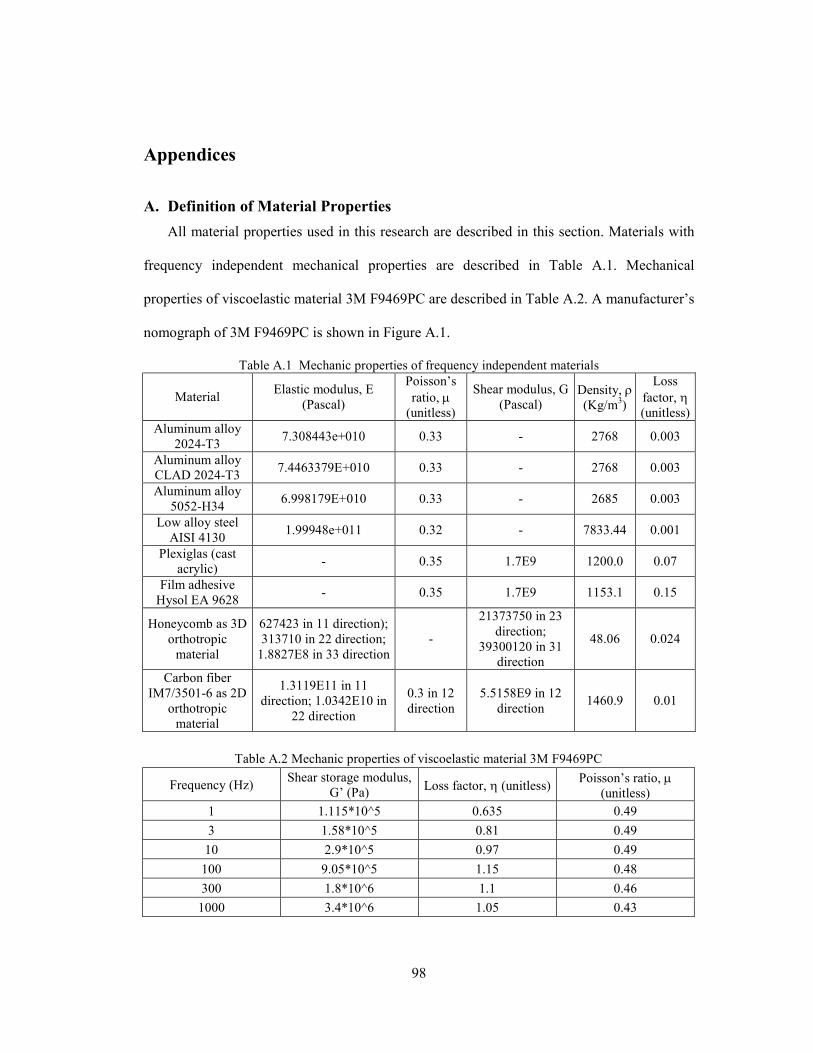
98

Appendices

A. Definition of Material Properties

All material properties used in this research are described in this section. Materials with

frequency independent mechanical properties are described in Table A.1. Mechanical

properties of viscoelastic material 3M F9469PC are described in Table A.2. A manufacturer’s

nomograph of 3M F9469PC is shown in Figure A.1.

Table A.1 Mechanic properties of frequency independent materials

Material Elastic modulus, E

(Pascal)

Poisson’s

ratio, µ

(unitless)

Shear modulus, G

(Pascal) Density, ρ

(Kg/m3)

Loss

factor, η

(unitless)

Aluminum alloy

2024-T3 7.308443e+010 0.33 - 2768 0.003

Aluminum alloy

CLAD 2024-T3 7.4463379E+010 0.33 - 2768 0.003

Aluminum alloy

5052-H34 6.998179E+010 0.33 - 2685 0.003

Low alloy steel

AISI 4130 1.99948e+011 0.32 - 7833.44 0.001

Plexiglas (cast

acrylic) - 0.35 1.7E9 1200.0 0.07

Film adhesive

Hysol EA 9628 - 0.35 1.7E9 1153.1 0.15

Honeycomb as 3D

orthotropic

material

627423 in 11 direction);

313710 in 22 direction;

1.8827E8 in 33 direction

-

21373750 in 23

direction;

39300120 in 31

direction

48.06 0.024

Carbon fiber

IM7/3501-6 as 2D

orthotropic

material

1.3119E11 in 11

direction; 1.0342E10 in

22 direction

0.3 in 12

direction

5.5158E9 in 12

direction 1460.9 0.01

Table A.2 Mechanic properties of viscoelastic material 3M F9469PC

Frequency (Hz) Shear storage modulus,

G’ (Pa) Loss factor, η (unitless)

Poisson’s ratio, µ

(unitless)

1 1.115*10^5 0.635 0.49

3 1.58*10^5 0.81 0.49

10 2.9*10^5 0.97 0.49

100 9.05*10^5 1.15 0.48

300 1.8*10^6 1.1 0.46

1000 3.4*10^6 1.05 0.43

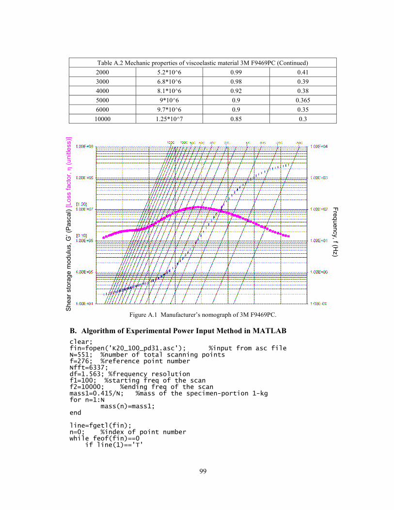
99

Table A.2 Mechanic properties of viscoelastic material 3M F9469PC (Continued)

2000 5.2*10^6 0.99 0.41

3000 6.8*10^6 0.98 0.39

4000 8.1*10^6 0.92 0.38

5000 9*10^6 0.9 0.365

6000 9.7*10^6 0.9 0.35

10000 1.25*10^7 0.85 0.3

Figure A.1 Manufacturer’s nomograph of 3M F9469PC.

B. Algorithm of Experimental Power Input Method in MATLAB

clear; fin=fopen('K20_100_pd31.asc'); %input from asc file N=551; %number of total scanning points f=276; %reference point number Nfft=6337; df=1.563; %frequency resolution f1=100; %starting freq of the scan f2=10000; %ending freq of the scan mass1=0.415/N; %mass of the specimen-portion 1-kg for n=1:N mass(n)=mass1; end line=fgetl(fin); n=0; %index of point number while feof(fin)==0 if line(1)=='T'

Shear sto

rage m

odulu

s, G

’ (P

ascal) [Loss facto

r, η

(unitle

ss)]

Fre

quency, f (H

z)

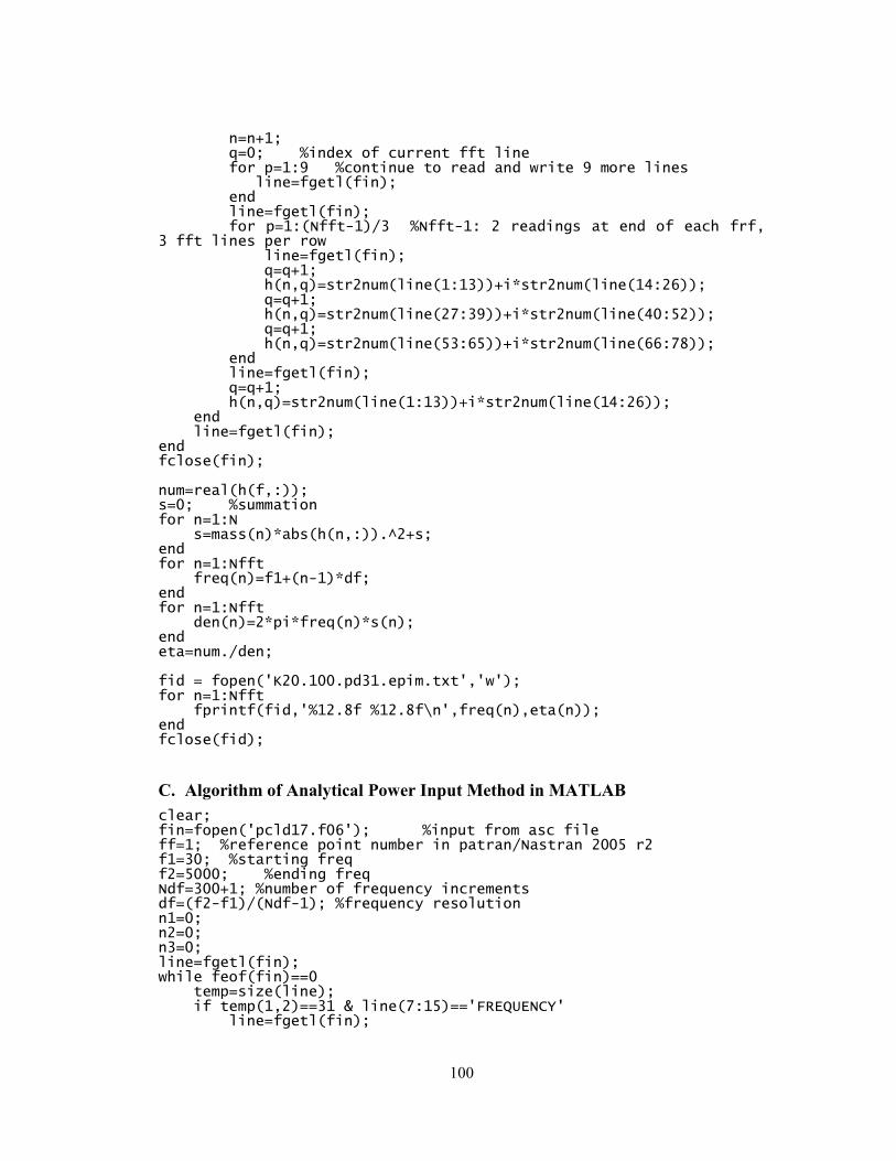
100

n=n+1; q=0; %index of current fft line for p=1:9 %continue to read and write 9 more lines line=fgetl(fin); end line=fgetl(fin); for p=1:(Nfft-1)/3 %Nfft-1: 2 readings at end of each frf, 3 fft lines per row line=fgetl(fin); q=q+1; h(n,q)=str2num(line(1:13))+i*str2num(line(14:26)); q=q+1; h(n,q)=str2num(line(27:39))+i*str2num(line(40:52)); q=q+1; h(n,q)=str2num(line(53:65))+i*str2num(line(66:78)); end line=fgetl(fin); q=q+1; h(n,q)=str2num(line(1:13))+i*str2num(line(14:26)); end line=fgetl(fin); end fclose(fin); num=real(h(f,:)); s=0; %summation for n=1:N s=mass(n)*abs(h(n,:)).^2+s; end for n=1:Nfft freq(n)=f1+(n-1)*df; end for n=1:Nfft den(n)=2*pi*freq(n)*s(n); end eta=num./den; fid = fopen('K20.100.pd31.epim.txt','w'); for n=1:Nfft fprintf(fid,'%12.8f %12.8f\n',freq(n),eta(n)); end fclose(fid);

C. Algorithm of Analytical Power Input Method in MATLAB

clear; fin=fopen('pcld17.f06'); %input from asc file ff=1; %reference point number in patran/Nastran 2005 r2 f1=30; %starting freq f2=5000; %ending freq Ndf=300+1; %number of frequency increments df=(f2-f1)/(Ndf-1); %frequency resolution n1=0; n2=0; n3=0; line=fgetl(fin); while feof(fin)==0 temp=size(line); if temp(1,2)==31 & line(7:15)=='FREQUENCY' line=fgetl(fin);

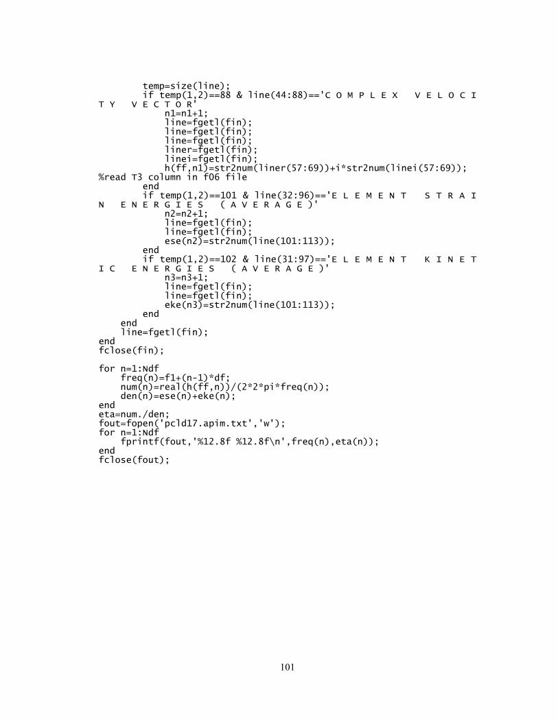
101

temp=size(line); if temp(1,2)==88 & line(44:88)=='C O M P L E X V E L O C I T Y V E C T O R' n1=n1+1; line=fgetl(fin); line=fgetl(fin); line=fgetl(fin); liner=fgetl(fin); linei=fgetl(fin); h(ff,n1)=str2num(liner(57:69))+i*str2num(linei(57:69)); %read T3 column in f06 file end if temp(1,2)==101 & line(32:96)=='E L E M E N T S T R A I N E N E R G I E S ( A V E R A G E )' n2=n2+1; line=fgetl(fin); line=fgetl(fin); ese(n2)=str2num(line(101:113)); end if temp(1,2)==102 & line(31:97)=='E L E M E N T K I N E T I C E N E R G I E S ( A V E R A G E )' n3=n3+1; line=fgetl(fin); line=fgetl(fin); eke(n3)=str2num(line(101:113)); end end line=fgetl(fin); end fclose(fin); for n=1:Ndf freq(n)=f1+(n-1)*df; num(n)=real(h(ff,n))/(2*2*pi*freq(n)); den(n)=ese(n)+eke(n); end eta=num./den; fout=fopen('pcld17.apim.txt','w'); for n=1:Ndf fprintf(fout,'%12.8f %12.8f\n',freq(n),eta(n)); end fclose(fout);

experimental and analytical estimation of damping in beams ...

Documents