Experiment M4: Photoluminescence...Experiment M4: Photoluminescence II. Institute of Physics A, WTHR Aachen April 14, 2016 Contents 1 Introduction 3 2 Fundamentals 4 2.1 Quantum theory

Experiment M4:

Photoluminescence

II. Institute of Physics A, RWTH Aachen

April 14, 2016

Contents

1 Introduction 3

2 Fundamentals 4

2.1 Quantum theory of the light - mater interaction . . . . . . . . . . . 42.2 Optical transitions in the solid states . . . . . . . . . . . . . . . . . 52.3 Optical transitions in semi conductors . . . . . . . . . . . . . . . . . 72.4 Photoluminescence . . . . . . . . . . . . . . . . . . . . . . . . . . . 82.5 Optical spin orientation and polarised photoluminescence . . . . . . 82.6 Excitons . . . . . . . . . . . . . . . . . . . . . . . . . . . . . . . . 112.7 Temperature dependence of the PL-peaks . . . . . . . . . . . . . . . 12

3 Sample system 15

3.1 Zinc oxide (ZnO) . . . . . . . . . . . . . . . . . . . . . . . . . . . . 153.2 Gallium arsenide (GaAs) . . . . . . . . . . . . . . . . . . . . . . . . 16

4 Experimental setup 17

4.1 Laser . . . . . . . . . . . . . . . . . . . . . . . . . . . . . . . . . . . 194.2 Spectrometer . . . . . . . . . . . . . . . . . . . . . . . . . . . . . . 19

4.2.1 Di�raction grating . . . . . . . . . . . . . . . . . . . . . . . 194.2.2 CCD . . . . . . . . . . . . . . . . . . . . . . . . . . . . . . . 20

5 Conducting the experiment and tasks 23

5.1 Working with Lasers: Safety instructions . . . . . . . . . . . . . . . 235.2 Adjustment of the Laser beam . . . . . . . . . . . . . . . . . . . . . 23

1

Contents

5.3 Recording of PL-spectra: Spectrometer Software . . . . . . . . . . . 245.4 Temperature dependent measurements on ZnO . . . . . . . . . . . . 25

5.4.1 Measurements . . . . . . . . . . . . . . . . . . . . . . . . . . 255.4.2 Analysis of the measurements . . . . . . . . . . . . . . . . . 25

5.5 Polarisation measurements on GaAs . . . . . . . . . . . . . . . . . . 255.5.1 Conducting the measurements . . . . . . . . . . . . . . . . . 255.5.2 Analysis . . . . . . . . . . . . . . . . . . . . . . . . . . . . . 26

5.6 Tips and tricks for analysing spectra . . . . . . . . . . . . . . . . . 265.7 Remarks about the report . . . . . . . . . . . . . . . . . . . . . . . 28

6 Questions for self-control 29

2

Required knowlege:

• Quantum mechanics of the interaction of light and matter, Fermi's goldenrule, perturbation theory.

• Semiconductor band structure, doping

• Excitons

• Laser, 4-level-system

• Light di�raction by a grating

1 Introduction

In spectroscopy, frequency and intensity of emitted, absorbed or re�ected radia-tion are analysed. By this, information about the interaction between radiationan matter, and their electronic structure are gained. Historically, spectroscopywas mainly con�ned to visible light which was emitted or absorbed by atoms andmolecules. Nowadays, spectroscopy ranges over a wide range of frequencies and isused to gain insight in the electronic structure of a material (emission or absorptionof photons), phonons in the solid state (Raman spectroscopy), crystal structure(X-Ray di�raction), core spins and structure of individual atoms or molecules(NMR), and many other material properties.

Luminescence describes the radiation emitted by a material which originatesfrom the transition of the system from an excited state into the ground state.In the case of Photo luminescence the excitation is induced optically by theabsorption of photons.In photo luminescence spectroscopy, electrons are optically excited into a level farabove the band edge. Subsequently, the electrons relax to the band minimumand emit luminescence radiation. The spectral composition of this light can giveinformation about the sort of states at the band edge, transition probabilities ore.g. vacancies and impurities

3

2 Fundamentals

2 Fundamentals

2.1 Quantum theory of the light - mater interaction

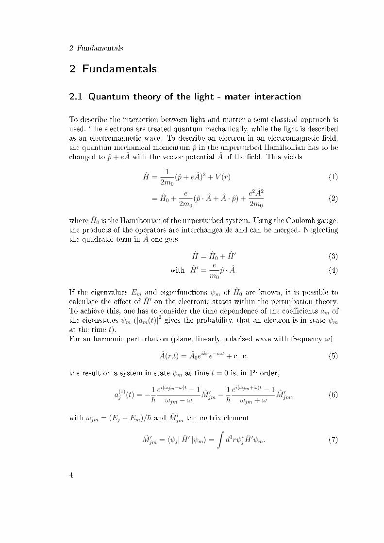
To describe the interaction between light and matter a semi classical approach isused. The electrons are treated quantum mechanically, while the light is describedas an electromagnetic wave. To describe an electron in an electromagnetic �eld,the quantum mechanical momentum p in the unperturbed Hamiltonian has to bechanged to p+ eA with the vector potential A of the �eld. This yields

H =1

2m0

(p+ eA)2 + V (r) (1)

= H0 +e

2m0

(p · A+ A · p) +e2A2

2m0

(2)

where H0 is the Hamiltonian of the unperturbed system. Using the Coulomb gauge,the products of the operators are interchangeable and can be merged. Neglectingthe quadratic term in A one gets

H = H0 + H ′ (3)

with H ′ =e

m0

p · A. (4)

If the eigenvalues Em and eigenfunctions ψm of H0 are known, it is possible tocalculate the e�ect of H ′ on the electronic states within the perturbation theory.To achieve this, one has to consider the time dependence of the coe�cients am ofthe eigenstates ψm (|am(t)|2 gives the probability, that an electron is in state ψmat the time t).For an harmonic perturbation (plane, linearly polarised wave with frequency ω)

A(r,t) = A0eikre−iωt + c. c. (5)

the result on a system in state ψm at time t = 0 is, in 1st order,

a(1)j (t) = −1

h

ei(ωjm−ω)t − 1

ωjm − ωM ′

jm −1

h

ei(ωjm+ω)t − 1

ωjm + ωM ′

jm, (6)

with ωjm = (Ej − Em)/h and M ′jm the matrix element

M ′jm = 〈ψj| H ′ |ψm〉 =

∫d3rψ∗j H

′ψm. (7)

4

2.2 Optical transitions in the solid states

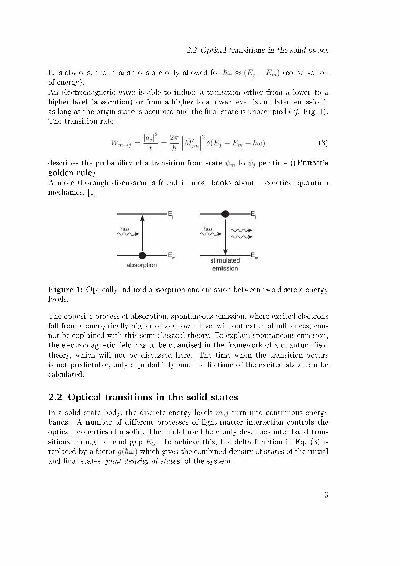
It is obvious, that transitions are only allowed for hω ≈ (Ej − Em) (conservationof energy).An electromagnetic wave is able to induce a transition either from a lower to ahigher level (absorption) or from a higher to a lower level (stimulated emission),as long as the origin state is occupied and the �nal state is unoccupied (cf. Fig. 1).The transition rate

Wm→j =|aj|2

t=

2π

h

∣∣∣M ′jm

∣∣∣2 δ(Ej − Em − hω) (8)

describes the probability of a transition from state ψm to ψj per time ((Fermi'sgolden rule).A more thorough discussion is found in most books about theoretical quantummechanics. [1]

Ej

Em

ħω

absorption

Ej

Emstimulatedemission

ħω

Figure 1: Optically induced absorption and emission between two discrete energylevels.

The opposite process of absorption, spontaneous emission, where excited electronsfall from a energetically higher onto a lower level without external in�uences, can-not be explained with this semi classical theory. To explain spontaneous emission,the electromagnetic �eld has to be quantised in the framework of a quantum �eldtheory, which will not be discussed here. The time when the transition occursis not predictable, only a probability and the lifetime of the excited state can becalculated.

2.2 Optical transitions in the solid states

In a solid state body, the discrete energy levels m,j turn into continuous energybands. A number of di�erent processes of light-matter interaction controls theoptical properties of a solid. The model used here only describes inter band tran-sitions through a band gap EG. To achieve this, the delta function in Eq. (8) isreplaced by a factor g(hω) which gives the combined density of states of the initialand �nal states, joint density of states, of the system.

5

2 Fundamentals

The simple density of states (DOS) of an electron in a parabolic band is identicalto the DOS of a free electron where the electron mass, me, is replaced by thee�ective mass m∗.

g(E) =1

2π

(2m∗

h2

) 32

E12 (9)

For the description of inter band transitions, the DOS of electrons and holes inparabolic bands are combined (see e.g. [2]) and it is,

g(hω) = 0 for hω < EG (10)

g(hω) =1

2π2

(2µ

h2

) 32

(hω − EG)12 for hω > EG (11)

with the reduced electron-hole-mass

1

µ=

1

m∗e+

1

m∗h. (12)

In Addition to the combined DOS, the transition-matrix element M ′jm (cf. equation

8) is the leading factor. This will be shown, looking at an interband transition ina solid.The eikr-term in eq. 5 is expanded into a Taylor expansion to

eikr = 1 + ik · r +1

2(ik · r)2 + . . . . (13)

For the interaction of electromagnetic waves with a wavelength in the order ofvisible light (λ ≈ 1µm) with atoms whose diameters are in the order of 10−10 m,only the �rst term has to be used as |k · r| ≈ 10−3. This approximation is calledthe electrical dipol approximation.The matrix element simpli�es to

M ′jm =

2e

m0

〈ψj| p · A0 |ψm〉 . (14)

The transitions of the outer valence band (vb) and the conduction bands (cb) in asolid are described by Bloch-waves

ψvb,cb(r) =1√V· uvb,cb(r) · eikvb,cb·r, (15)

where uvb,cb(r) are lattice periodic functions.

6

2.3 Optical transitions in semi conductors

By looking at a transition, induced by a photon with kopt from the valence- to theconduction band and replacing the ψj,m in equation (14) with Bloch-waves, it isshown that there is a contribution only for kvb = kcb − kopt. As the wave vectorof the electrons is some orders of magnitude larger that the momentum of thephoton, one gets

kvb ≈ kcb. (16)

This shows, that the wave vector of the electron stays approximately constant andonly 'straight' transitions in the E(k) diagram are possible.If an electric dipole transition is possible does not only depend on the energy andmomentum of the respective states. A quantum mechanical consideration of dipoltransitions of electrons within an hydrogen atom which is characterised with thequantum numbers n, l, ml and ms yields the following selection rules

• ∆ml = 0,± 1.

• ∆l = ±1. The total momentum of electron and photon (±1) is conserved.

• ∆ms = 0. Spin conservation.

These rules are also applicable to atoms with many electrons, or solids, where theelectronic states are described by atomic wave functions.In transitions which are forbidden by the selection rules, magnetic dipole or quadrupoletransitions may occur which result from the higher order terms in eq. 13. The tran-sitions have considerably lower transition probabilities and happen on a longer timescale (10−6 s). Slow emission due to these transitions is called phosphorescence.Emissions due to inter-band recombinations of electron-hole pairs happen on amuch shorter time scale (10−9 to 10−8 s). This process is called �uorescence.

2.3 Optical transitions in semi conductors

Due to their band structure, semiconductors are separated in two sub categories.In a direct semiconductor (e.g. GaAs, GaN, ZnO) the maximum of the valenceband (VB) and the minimum of the conduction band (CB) are "above one other"in momentum space with identikal k = 0. Optical transitions for valende bandelectrons into the conduction band are hence possible under eq. 16, as soon as thephoton energy ful�ls hω > EG.Usually the CB minimum is not in the centre of the Brillouin zone, but at k 6= 0.Due to eq. 16, and as shown in Fig. 2, direct transitions are not possible. Thedi�erence in momentum between VB maximum and CB minimum have to becompensated by an additional emission or absorption of phonons. These are calledindirect semiconductors (e.g. Si).In real semiconductors a number of optical transitions occur at energies below

7

2 Fundamentals

Valence band

Conduction band

kk = 0

Ea)

ħω

Valence band

Conduction band

kk = 0

Eb)

ħωPhonon

EGEG

Figure 2: Transitions from valence to condution band in a a) direct and b) indirectsemi conductor.

EG. Possible reasons are e.g. doping or defects such as impurities, vacanciesor interstitial atoms. These local disturbances yield discrete energy levels whichusually reside just above the VB (e.g. acceptor levels) or below the CB (e.g. donorlevels).Another e�ect leading to a sharp absorption peak below the band edge in manymaterials is the excitation of exciton. This will be discussed in Section 2.6.

2.4 Photoluminescence

Photoluminescence is the process of emitting radiation by spontaneous recombi-nation of an optically excited photon. This usually happens with photon energyhω > EG where an electron-hole pair with momentum hk 6= 0 is created (cf.Fig. 3). Due to strong electron phonon coupling, these 'hot' electrons relax, byemitting a photon, to the minimum of the CB. This process takes place on veryfast times cales ≈ 100 fs. It can hence be assumed, that most electrons are com-pletely relaxed prior to recombination via an inter band transition (order of 10−9

to 10−8 s).The same holds for holes, which relax to the VB maximum before recombiningwith an electron from the CB at k = 0.

2.5 Optical spin orientation and polarisedphotoluminescence

The photoluminescence of a sample can also be used to gain infromation aboutthe spin properties of the excited electrons, see Fig. 10. The basic principlesof this are the selection rules discussed in section 2.3 which couple the spin ofthe excited electrons to the polarisation of the photons. The optical excitation

8

2.5 Optical spin orientation and polarised photoluminescence

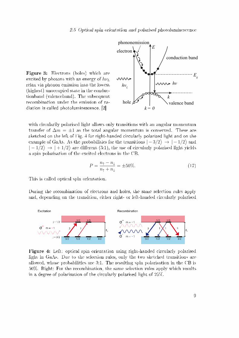
Figure 3: Electrons (holes) which areexcited by photons with an energy of hνLrelax via phonon emission into the lowest(highest) unoccupied state in the conduc-tionband (valenceband). The subsequentrecombination under the emission of ra-diation is called photoluminescence. [2]

E

hν

k = 0

k

conduction band

valence band

hνL

Eg

electron

hole

phononemission

with circularily polarised light allows only transitions with an angular momentumtransfer of ∆m = ±1 as the total angular momentum is conserved. These aresketched on the left of Fig. 4 for right-handed circularly polarised light and on theexample of GaAs. As the probabilities for the transitions |− 3/2

⟩→ |− 1/2

⟩and

| − 1/2⟩→ |+ 1/2

⟩are di�erent (3:1), the use of circularly polarised light yields

a spin polarisation of the excited electrons in the CB.

P =n↑ − n↓n↑ + n↓

= ±50%. (17)

This is called optical spin orientation.

During the recombination of electrons and holes, the same selection rules applyand, depending on the transition, either right- or left-handed circularly polarised

Figure 4: Left: optical spin orientation using right-handed circularly polarisedlight in GaAs. Due to the selection rules, only the two sketched transitions areallowed, whose probabilities are 3:1. The resulting spin polarisation in the CB is50%. Right: For the recombination, the same selection rules apply which resultsin a degree of polarisation of the circularly polarised light of 25%.

9

2 Fundamentals

light is emitted. As before, the di�erent probabilities have to be taken into account(cf. Fig. 4 right hand side) which yields a degree of polarisation of the PL light of

Pcirc =I+ − I−I+ + I−

= ±25% (18)

after the excitation of an electron spin polarisation of 50% due to circularly po-larised light. Generally the degree of polarisation of the PL-light can be attributedto the spin polarisation of excited CB electrons.

10

2.6 Excitons

2.6 Excitons

Electrons and holes, which are generated by the absorption of photons, are spa-tially at the same place in the solid. Oppositely charged, they attract each otherdue to Coulomb interactions. This may yield bound, hydrogen-like states of theelectron-hole pair which are called exciton.Excitons are be split in two main categories: Wannier-Mott- and Frenkel-excitons.Wannier-Mott-excitons are weakly bound electron-hole pairs with a large ra-dius which mainly occur in semiconductors. The binding energy is calculated inaccordance with Bohr's model of the hydrogen atom. The high dielectric constantεr of the medium in which the exciton exists has to be taken into account. Thereduced mass of the proton and electron 1/µ = 1/m∗

e + 1/m∗h are replaced by the

e�ective mass of electron and hole in the solid. This yields:

En = − µ

me

1

ε2r

RH

n2= −RX

n2(19)

with the Rydberg constant RH = 13,6 eV. The radius of the exciton is

rn =me

µεrn

2aB = n2aX , (20)

where aB is the Bohr radius of the hydrogen atom.Typical binding energies and radii are shown in Fig. 5. Note that Wannier-Mott-excitons stretch over many lattice constants. As they are able to movefreely through the solid, these excitons are called free excitons.Frenkel-excitons on the other hand are strong bound and have small radii inthe order of the lattice parameter. Due to their smaller size, the assumption ofa homogeneous material is not valid any more and the surrounding of the ecitionhas to be taken into account as well. Hence, the model in eq. 19 cannot be usedanymore to calculate the binding strength. Experimentally one gets values of acouple of 10meV up to 1 eV in some organic semiconductors.Bound excitons form when a free exciton binds to a defect or donor atom, eherebyit gains more energy.

For the optical properties of semiconductors excitoons play an important role, asthey often dominate the absorption spectrum just below the band edge. Electronsare able to be excited into the CB although the photon energy is not su�cient,the missing energy is taken from the binding energy of the exciton.In many materials, excitons are only observable at low temperatures as for theformation of stable excitons the binding energy needs to be higher than the thermal

11

2 Fundamentals

Figure 5: Band gap Eg,excitonic Rydberg-constantRX and exciton-Bohr-radiusaX of some semiconductorsfrom [2].

energy of the phonons in the material.

2.7 Temperature dependence of the PL-peaks

The temperature dependence of the PL intensity of exciton peaks is explained bythe equation for the rate equation for the exciton population.

dNX

dt= G− (γr + γnr)NX . (21)

Here, NX is the number or density of the excitons in question and G the excitationrate thereof. γr and γnr are the rates for radiative (r) and non-radiative (nr)transitions. In equilibration dNX/dt = 0 one gets the equilibrium population

NX =G

γr + γnr. (22)

The intensity of the PL-peaks is obviously given by the radiating transitions,

I(T ) = γr ·Nx =γr

γr + γnr·G. (23)

The temperature dependence of the PL-intensity is in the transition rates γr andγnr. The non-radiative transitions describe transitions from one excitonic stateinto another and can be modelled by a Boltzman-factor,

γnr = γ0nr · e

− δEkBT , (24)

12

2.7 Temperature dependence of the PL-peaks

while the radiative transitions, e.g. the recombination processes, which emit PL-light, can be approximated as independent of temperature,

γr = γ0r = const. (25)

δE is the energy di�erence between the initial and �nal excitonic state of the non-radiative transitions. Inserting this term in eq. 23, this yields the temperaturedependence of the PL-intensity

I(T ) =I0

1 + γ · e−δEkBT

(26)

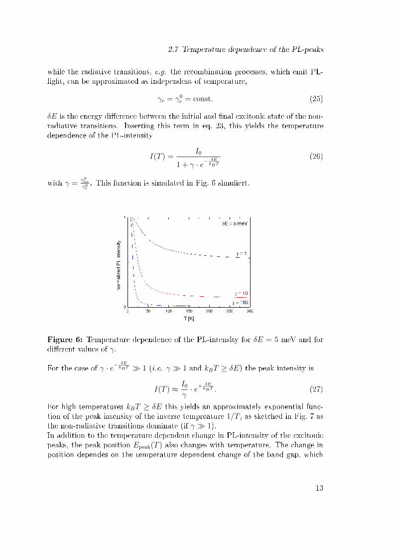
with γ = γ0nrγ0r. This function is simulated in Fig. 6 simuliert.

Figure 6: Temperature dependence of the PL-intensity for δE = 5 meV and fordi�erent values of γ.

For the case of γ · e−δEkBT � 1 (i.e. γ � 1 and kBT ≥ δE) the peak intensity is

I(T ) ≈ I0

γ· e+ δE

kBT . (27)

For high temperatures kBT ≥ δE this yields an approximately exponential func-tion of the peak intensity of the inverse tempreature 1/T , as sketched in Fig. 7 asthe non-radiative transitions dominate (if γ � 1).In addition to the temperature dependent change in PL-intensity of the excitonicpeaks, the peak position Epeak(T ) also changes with temperature. The change inposition dependes on the temperature dependent change of the band gap, which

13

2 Fundamentals

Figure 7: Temperature dependence of the PL-intensity for δE = 5 meV and fordi�erent values of γ. For high temperatures this is an almost exponential functionof the intensity of inverse temperature 1/T , as γ � 1.

is described by the phenomenological Varshni-formula [3]

Eg(T ) = Eg(T = 0K)− α T 2

T + β. (28)

Herem α and β are meterial speci�c constants. For the exciton energies this yieldsEpeak(T ) = Eg(T ) − Eb with the total binding energy of the excitons Eb. Thelatter resembles the binding energies of an electron and a hole of a free exciton, aswell as additional contributions due to the localisation of the exciton at a defectsite.

14

3 Sample system

3.1 Zinc oxide (ZnO)

Zinc oxide as a II-VI-semiconductor of great scienti�c interest (cf. [4] as an overview).Due to its large band gap of EG = 3,44 eV it is ideal for opto-electronic devices inthe near UV-range as e.g. blue LEDs.The emission spectrum of ZnO is dominated by excitons, whose binding energyof 60meV is well above the thermal energy at room temperature (≈ 25meV) andhence yields the possibility to use ZnO for Lasers or LEDs based on excitonicemission, which would have very narrow de�ned energies.As ZnO is easily n-doped with e.g. Aluminum and is transparent to visible light, itis also ideal as transparent conducting layer (TCO, transparent conducting oxide).These are used in touch-screens or �at-screens or as a front electrode for solar cells,where the otherwise occurring shading is omitted.

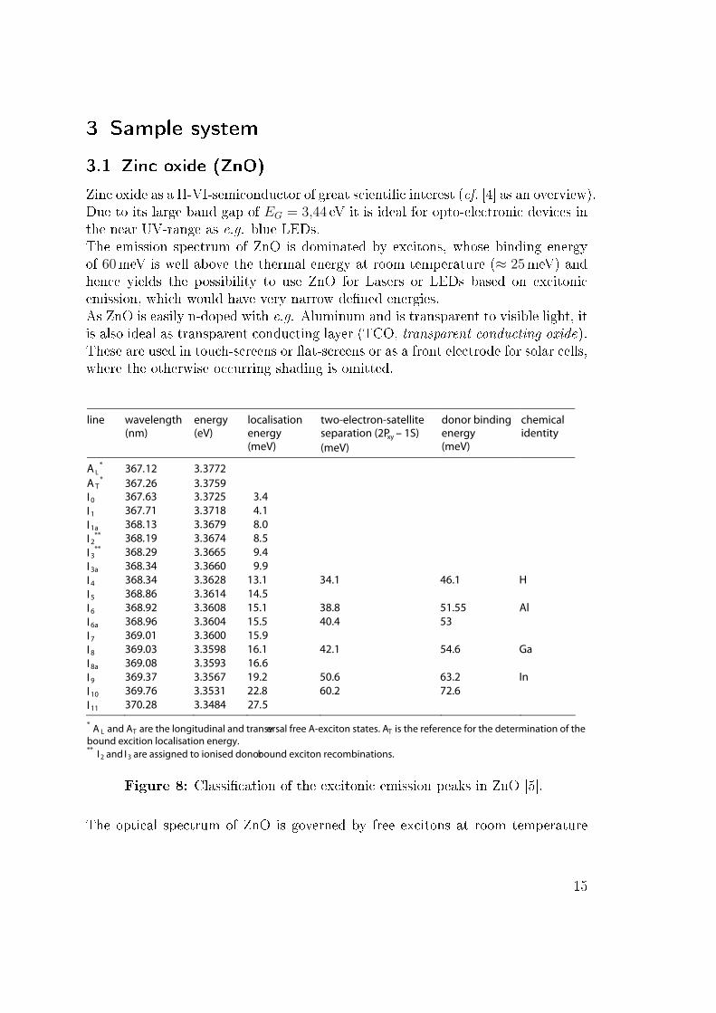
line wavelength (nm)

energy (eV)

localisation energy (meV)

two-electron-satellite separation (2Pxy – 1S) (meV)

donor binding energy (meV)

chemical identity

A L* 2773.3 21.763

A T* 9573.3 62.763

I0 4.3 5273.3 36.763I 1 1.4 8173.3 17.763I 1a 0.8 9763.3 31.863I 2

** 5.8 4763.3 91.863I 3

** 4.9 5663.3 92.863I 3a 9.9 0663.3 43.863I 4 368.34 3.3628 13.1 34.1 46.1 H I5 5.41 4163.3 68.863I 6 368.92 3.3608 15.1 38.8 51.55 Al I6a 368.96 3.3604 15.5 40.4 53 I7 9.51 0063.3 10.963I 8 369.03 3.3598 16.1 42.1 54.6 Ga I8a 6.61 3953.3 80.963I9 369.37 3.3567 19.2 50.6 63.2 In I10 369.76 3.3531 22.8 60.2 72.6 I11 5.72 4843.3 82.073

* A L and AT are the longitudinal and transversal free A-exciton states. AT is the reference for the determination of the bound excition localisation energy. ** I2 and I3 are assigned to ionised donor bound exciton recombinations.

Figure 8: Classi�cation of the excitonic emission peaks in ZnO [5].

The optical spectrum of ZnO is governed by free excitons at room temperature

15

3 Sample system

<111> <100>

Γ-Minimum

light holes

split-off holes

Eg

k

Ene

rgy

0 100 200 3001.2

1.3

1.4

1.5

1.6

Temperature [K]

Ene

rgy

[eV

]

Eg

heavy holes

Figure 9: Band structure of GaAs and the temperature dependence of the bandgap energy.

and by a number of emission lines originating from bound excitons at low tempera-tures. Depending on the sample, up to eleven di�erent lines are observable. Theseresult mainly from excitons which are bound to neutral or ionised donor atoms. Athorough assessment and characterisation of the lines was done by Meyer et al.. [5]A summary of results is shon in the table in Fig. 8. The localisation energies of thebound excitons, which add to the binding energies of free excitons of ≈ 60meV,are in the order of a few meV. This explains why bound excitons are only stableat low temperatures.

Some of the lines are attributed to certain elements to which the excitons arebound. A PL-measurement on ZnO can hence give an insight in the used donoratoms.

The sample to be examined consists of a some hundred of nm thick pulsed laser

deposition (PLD) grown thin �lm on a saphire substrate.

3.2 Gallium arsenide (GaAs)

Gallium arsenide is a III-V semiconductor with a direct bandgap of Eg = 1,42 eVat T = 300 K (cf. Fig. 9). The material is of high technological relevance. It isespecially prominent for its long spin lifetimes of over 100 ns at low temperaturesand ideal doping at the metal-insulator transition of n(Si) ≈ 3 · 1016 cm−3 in spinelectronic. [6, 7].

16

4 Experimental setup

HeC

d-U

V-La

ser

IR-d

iode

Las

er

Cry

osta

t

Sample

CC

D

Spectrometer

Optical fibre

Pol.LCVR

Pol.

LCVR

Filte

r whe

el

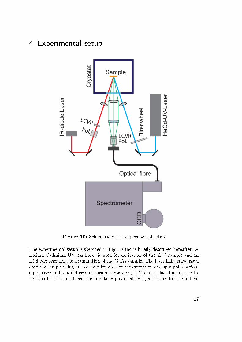
Figure 10: Schematic of the experimental setup

The experimental setup is sketched in Fig. 10 and is brie�y described hereafter. AHelium-Cadmium UV gas Laser is used for excitation of the ZnO sample and anIR diode laser for the examination of the GaAs sample. The laser light is focussedonto the sample using mirrors and lenses. For the excitation of a spin polarisation,a polariser and a liquid crystal variable retarder (LCVR) are placed inside the IRlight path. This produced the circularly polarised light, necessary for the optical

17

4 Experimental setup

5s 12

5p 12

5p 32

5s2 32

5s2 52

Ground stateof the Cd2+ ion

441.6 nm

325.0 nm

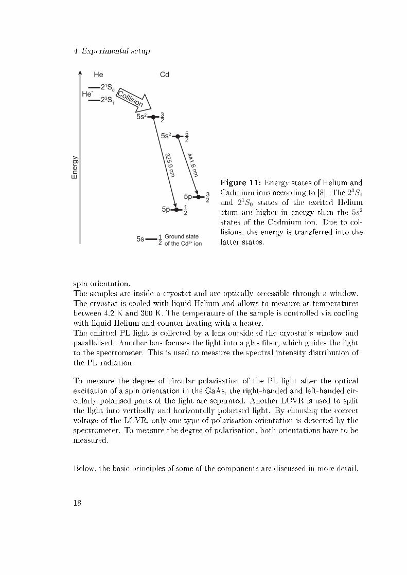
CdHe

23S1

21S0He*

Ene

rgy

Collision

Figure 11: Energy states of Helium andCadmium ions according to [8]. The 23S1

and 21S0 states of the excited Heliumatom are higher in energy than the 5s2

states of the Cadmium ion. Due to col-lisions, the energy is transferred into thelatter states.

spin orientation.The samples are inside a cryostat and are optically accessible through a window.The cryostat is cooled with liquid Helium and allows to measure at temperaturesbetween 4.2 K and 300 K. The temperature of the sample is controlled via coolingwith liquid Helium and counter heating with a heater.The emitted PL light is collected by a lens outside of the cryostat's window andparallelised. Another lens focuses the light into a glas �ber, which guides the lightto the spectrometer. This is used to measure the spectral intensity distribution ofthe PL radiation.

To measure the degree of circular polarisation of the PL light after the opticalexcitation of a spin orientation in the GaAs, the right-handed and left-handed cir-cularly polarised parts of the light are separated. Another LCVR is used to splitthe light into vertically and horizontally polarised light. By choosing the correctvoltage of the LCVR, only one type of polarisation orientation is detected by thespectrometer. To measure the degree of polarisation, both orientations have to bemeasured.

Below, the basic principles of some of the components are discussed in more detail.

18

4.1 Laser

4.1 Laser

As excitation source for the measurements in the UV a HeCd gas laser is used. Theactive medium is a Helium and Cadmium metal vapour mixture. The He atomsare excited via gas discharge and give the energy to the Cd atoms via collisions.The Cd atoms are now ionised and excited. The radiative recombination producesthe characteristic Laser line wavelengths. The dominant transitians are from the5s to the 5p level (cf. Fig. 11) which belong to emission lines at λ = 325 nm andλ = 442 nm. The Laser used here emitts the energetically higher wavelength of325 nm.For the polarisation dependent measurements on GaAs a GaAs/GaAlAs diodelaser is used. This emits light between 808.4 nm and 812.9 nm. The power iscontrolled by limiting the current on the controller. The exact principles of a lasercan be found in the instructions for the lab-course "Nd-YAG-Laser".

4.2 Spectrometer

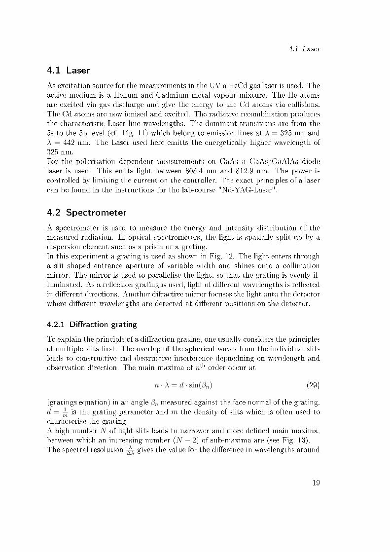
A spectrometer is used to measure the energy and intensity distribution of themeasured radiation. In optical spectrometers, the light is spatially split up by adispersion element such as a prism or a grating.In this experiment a grating is used as shown in Fig. 12. The light enters througha slit shaped entrance aperture of variable width and shines onto a collimationmirror. The mirror is used to parallelise the light, so that the grating is evenly il-luminated. As a re�ection grating is used, light of di�erent wavelengths is re�ectedin di�erent directions. Another difractive mirror focuses the light onto the detectorwhere di�erent wavelengths are detected at di�erent positions on the detector.

4.2.1 Di�raction grating

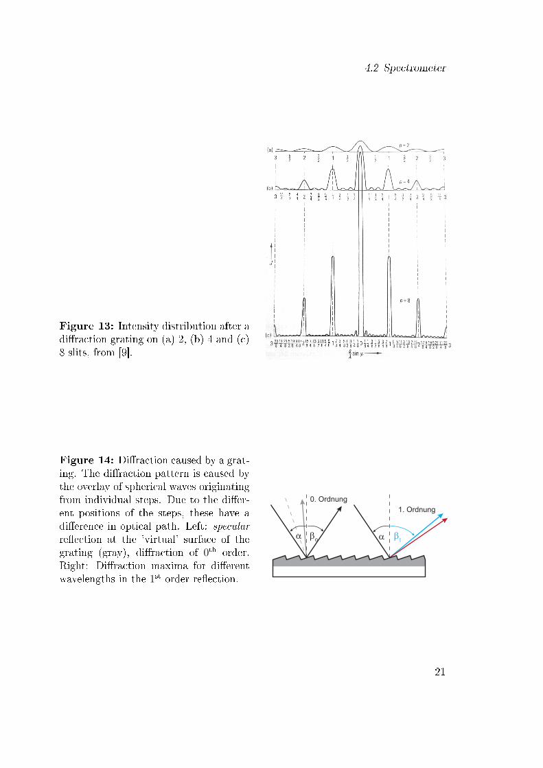
To explain the principle of a di�raction grating, one usually considers the principlesof multiple slits �rst. The overlap of the spherical waves from the individual slitsleads to constructive and destructive interference depnedning on wavelength andobservation direction. The main maxima of nth order occur at

n · λ = d · sin(βn) (29)

(gratings equation) in an angle βn measured against the face normal of the grating.d = 1

mis the grating parameter and m the density of slits which is often used to

characterise the grating.A high number N of light slits leads to narrower and more de�ned main maxima,between which an increasing number (N − 2) of sub-maxima are (see Fig. 13).The spectral resolution λ

∆λgives the value for the di�erence in wavelengths around

19

4 Experimental setup

Col

limat

ion

mirr

orFo

cuss

ing

mirr

or

reflectinggrating

Entrance slit

Detector surface

Figure 12: Schematics of the used spectrometer (Czerny-Turner-con�guration)

one main wavelength λ for two lines to be able to be separeted. For optical gratingsit is

λ

∆λ= nN. (30)

In the experiment a re�ection instead of a transmission grating is used as sketchedin Fig. 14 (b). In the most simple case, these are just a number of grooves in thematerial. However, usually one uses a saw-tooth pro�le to gain better results. Bytuning the angle of the saw-tooth, a high intensity for a certain wavelength and avertain order is achieved. This is called a blazed grating.The grating equation is corrected for the re�ective grating to

n · λ = d (sin(βn)− sin(α)) . (31)

Re�ection gratings have the advantage, that no intensity is lost via absorption atthe bars of the grating.

4.2.2 CCD

To record the light intensity as a function of wavelength, a charge-coupled device

(CCD) is used. CCDs are one- or two-dimensional sensors which are commonlyused in digital cameras. Fro their invention, W. Boyle and G. E. Smith won the

20

4.2 Spectrometer

Figure 13: Intensity distribution after adi�raction grating on (a) 2, (b) 4 and (c)8 slits, from [9].

Figure 14: Di�raction caused by a grat-ing. The di�raction pattern is caused bythe overlay of spherical waves originatingfrom individual steps. Due to the di�er-ent positions of the steps, these have adi�erence in optical path. Left: specularre�ection at the 'virtual' surface of thegrating (gray), di�raction of 0th order.Right: Di�raction maxima for di�erentwavelengths in the 1st order re�ection.

0. Ordnung

α β0 β1

1. Ordnung

α

21

4 Experimental setup

p-Si

10 V 5 V

10 V 15 VVG = 5 V

p-Si

a) b) VG = 5 V

Metal

InsulatorEF

VB

CB

hν

VG

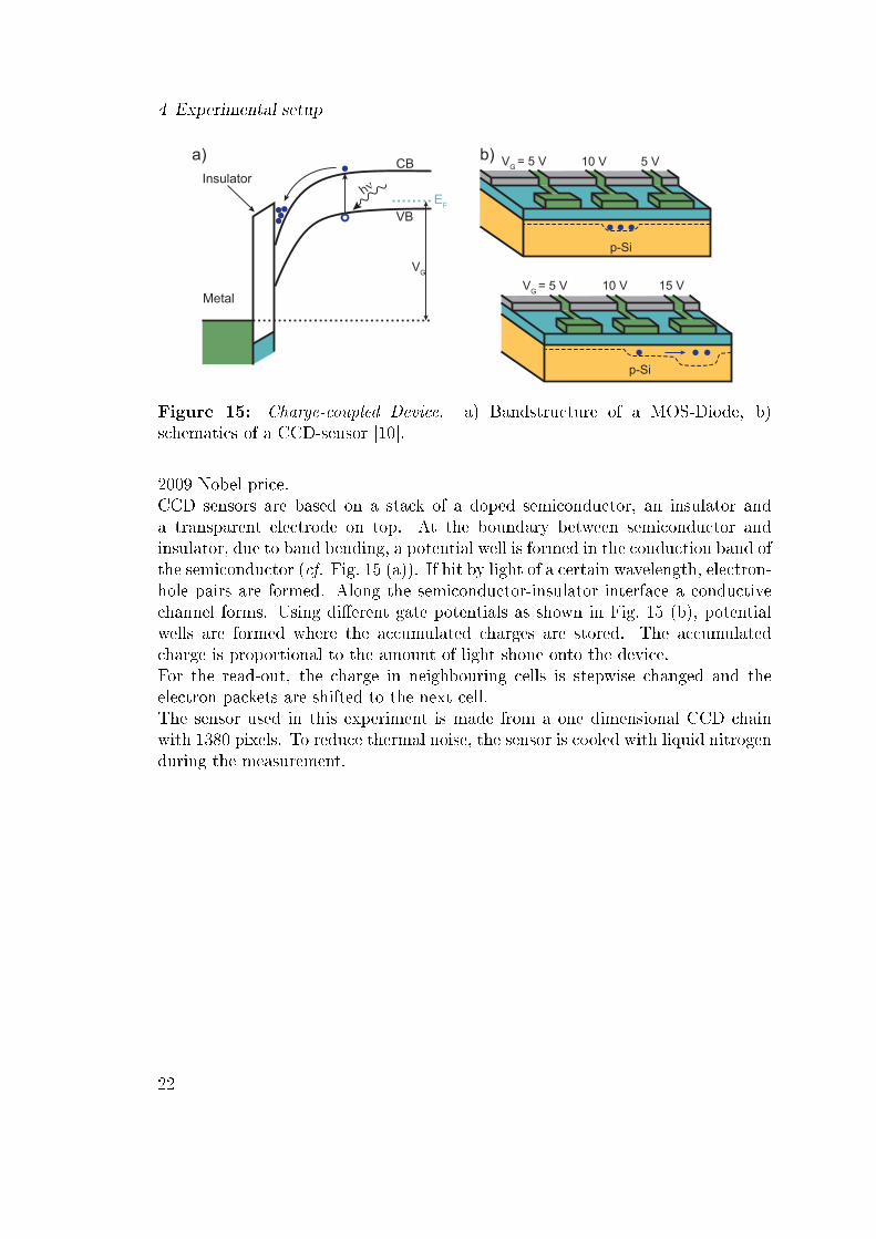
Figure 15: Charge-coupled Device. a) Bandstructure of a MOS-Diode, b)schematics of a CCD-sensor [10].

2009 Nobel price.CCD sensors are based on a stack of a doped semiconductor, an insulator anda transparent electrode on top. At the boundary between semiconductor andinsulator, due to band bending, a potential well is formed in the conduction band ofthe semiconductor (cf. Fig. 15 (a)). If hit by light of a certain wavelength, electron-hole pairs are formed. Along the semiconductor-insulator interface a conductivechannel forms. Using di�erent gate potentials as shown in Fig. 15 (b), potentialwells are formed where the accumulated charges are stored. The accumulatedcharge is proportional to the amount of light shone onto the device.For the read-out, the charge in neighbouring cells is stepwise changed and theelectron packets are shifted to the next cell.The sensor used in this experiment is made from a one dimensional CCD chainwith 1380 pixels. To reduce thermal noise, the sensor is cooled with liquid nitrogenduring the measurement.

22

5 Conducting the experiment and tasks

At the beginning of the day of the experiment the CCD-chip of the spectrometershould be cooled with liquid nitrogen under supervision of the tutor. During theoral exam, the temperature can begin to settle. Also the Laser should be switchedon to allow for stabilisation of the working temperature.

5.1 Working with Lasers: Safety instructions

The radiation emitted by the Lasers has a power of a couple 10 mW. Already muchlower power can irreparably damage the eyes! Always wear Laser safety glasseswhen the Lasers are switched on. This protects you from accidentally re�ectedradiation during adjustment of the light path. However, the glasses only partiallyblock the radiation. Even with glasse on:

Never look directly into the Laser beam!Never lower your head down to the hight of the Laser beam!

While working on the Laser beam remove all watches, rings, bracelets and otherre�ective objects which might cause re�ections. Be careful that the metallic Allenkeys or the optical holders never come into the light path. Always block the Laserwith a white card (or, in case of the UV Laser, the shutter) when adjusting theoptics.All optics cause back re�ections. Take extra care that all re�ections hit the blackshields around the setup and are not able to hit any metallic surface.

5.2 Adjustment of the Laser beam

The Laser beam should be aligned by the tutor in a way that they hit the sampleunder the same angle and thus be re�ected back in the same light path. Thisresults in a similar adjustment of the two beams. You should nevertheless controlthe alignment using the markings on the table and the calibration iris. To do so,adjust the Laser to a power of 1 mW and check for the correct hight of the beamand that all optics (such as mirrors, lenses and polarisers) are hit centrally. Toachieve the back re�ection in the same path, the cryostat, and hence the samples,might have to be rotated.

If using the Laser power meter the following rules apply:

• The λ-key is used to set the wavelength for which you wish to adjust thepower. Con�rm with "OK".

• The arrow keys change the range "R".

23

5 Conducting the experiment and tasks

We recommend to start with the ZnO measurements using the UV-Laser as thePL-light of ZnO is slightly blueish and visible to the eye. That eases the alignmentof the detection optics. To align the detection optics, you probably have to removethe safety glasses as these also shield the visible light. You should only do so if youare sure that the Laser beam is carefully adjusted and no metallic object can behit be the beam. After �nishing the adjustment you should use the safety glassesagain. Now hold the white card behind the collimation lens and move it towardsthe collimation lens for the �bre. Adjust the �bre in a way that it is centrally hitby the focused PL-light. A �ne adjustment can be made by optimising the peakheights of the recorded spectra.If swapping the Laser to IR, only very small adjustments to the �bre should benecessary to optimise the signal of the PL-spectra.

5.3 Recording of PL-spectra: Spectrometer Software

CCD and spectrometer are controlled and read-out by the software Syner JY V3.5

which is build into Origin. The software records spectra by measuring the CCDcounts per chosen time interval. You can change the settings in the menu

Collect → Experiment Setup.

The spectrometer has two di�erent gratings with di�erent parameters (lines/mm).The coarse grating has 120 lines/mm and a lower spectral resolution, but a widerspectral �eld which is recorded compared to the �ne grating with 1200 lines/mm.The latter has the better spectral resolution, but is only able to record a range ofabout 40 nm. However, for recording a high resolution spectrum, the �ne gratingcan still be used, as the software is able to stitch the spectra together. The gratingis chosen atMonos → Grating.The measuring range can be set in one of two ways: Either by choosing a centralwavelength (Detectors → CCD Position) or by choosing a start and end wave-length (Detectors → CCD Range). In the latter case, a number of spectra arerecorded and stitched together if the range is larger than the range of a singlespectrum. Make sure that the Laser wavelength is not in the set range, as the highintensity of the Laser might damage the CCD of the spectrometer.For the correct recording of PL-spectra the exposure time of the CCD sensor hasto be set viaDetectors → Exposure Time.After the change of experimental parameters such as Laser power, alignment orsample temperature, the exposure time has to be set to the lowest value (0.01 s)to avoid damage to the CCD sensor. The maximum signal the sensor can record

24

5.4 Temperature dependent measurements on ZnO

are 60000 counts. If necessary change the exposure time (up to a factor of 10)to use the maximum amount of counts and optimise the signal-noise ratio. How-ever, for all new settings, a background measurement should be recorded, wherethe Laser is blocked. This background can than be subtracted from the measureddata. Make sure that Detectors → Dark Substract is switched o�, as this wouldsubtract another, not �tting dark measurement which does not correspond to youractual measurement.

The software also allows the record of multiple spectra in a row and to averagethese. (Detectors → Accumulations resp. Detectors → Cycles) Recording a se-quence of measurements might be usefull during the �bre adjustment. If you donot want to use that function, set all values to '1'.The recorded spectra are presented as a graph and an Origin worksheet. You caneither work with the worksheets in Origin, or save these for another application.

5.4 Temperature dependent measurements on ZnO

5.4.1 Measurements

Investigate the temperature dependence of bound excitons in the existing ZnOsample. You should record PL-spectra between 10 k and 100 K in suitable tem-perature steps. Choose an appropriate range of wavelengths and set the exposuretime accordingly. After changing parameters, remember to record an additionalnoise measurement with identical settings for subtraction. For once, also recordone spectrum which shows the Laser wavelength with an exposure time of 0.01 s.This is to verify the calibration of the spectrometer.

5.4.2 Analysis of the measurements

Identify the individual exciton peaks of ZnO. Which impurities can be identi�ed?Analyse the temperature dependence of the peaks (peak height, width and posi-tion) and determine the localisation energies of the excitons.

5.5 Polarisation measurements on GaAs

5.5.1 Conducting the measurements

Set the sample temperature to 10 K. Change to the GaAs sample by aligning thecryostat horizontally and vertically so that the IR Laser beam hits the sample.Check the alignment of the �bre via maximising the peak heights in the PL spec-tra. To do so, record a couple of spectra without polarising optics (Polariser andLCVR).

25

5 Conducting the experiment and tasks

After �ne adjustment of the �bre, you have to set the voltage of LCVR wherelinearly polarised light is transformed to circularly poilarised light and vice versa.To set the LCVR voltage the driver with two LCVRs must be connected to thecomputer over USB and the program �LC Driver� must be started. The voltagesdriving both LCVRs can be set independently from each other. A λ/4 retardationcan be achieved at voltages Uσ+ = 1. 97 V and Uσ− = 4. 07 V. Place both polarisersin the incoming beam and adjust their optical axes to be parallel by measuring theLaser power behind the polarisers. When are the optical axes parallel? After that,place the second polariser and one of the LCVRs between the focussing lens andthe �bre in the detector area. Take care for the correct orientation with respectto the beam direction.Measure the degree of polarisation of the PL-light at 10 K. Remember to take anoise measurement.

5.5.2 Analysis

Identify the visible peaks in the circularly polarised light I+ and I− by a literatureresearch. Analyse and discuss the spectrum for the degree of circularly polarisa-tion of the PL-light according to eq. 18. Does this measurement show what youexpected?

5.6 Tips and tricks for analysing spectra

This section deals with some problems which might occur by analysing the spectraand how to avoid these.

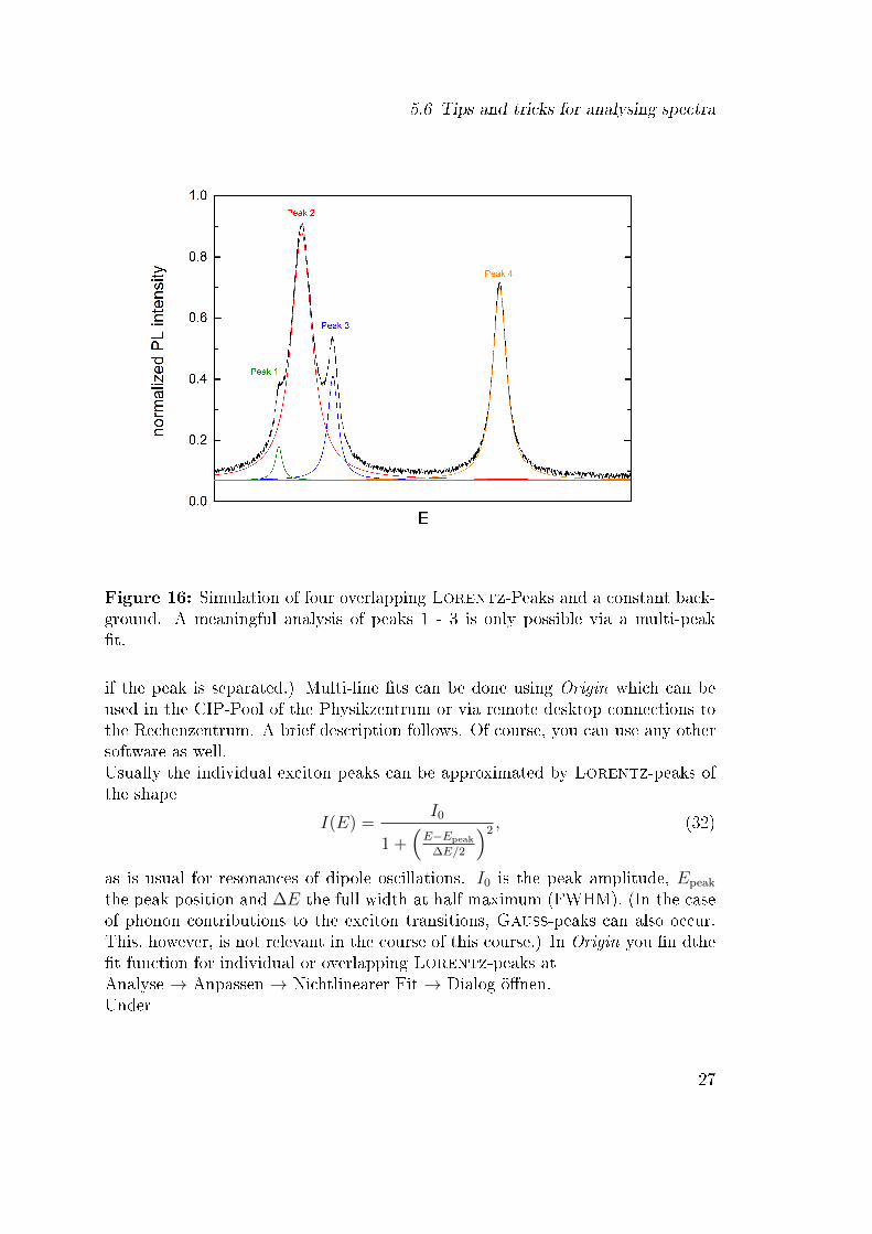
As shown in table 8 many excitonic transitions can lay very close together in thePL-spectra and even overlap. Figure 16 shows a simulation of four overlappingpeaks with a constant background. The individual peaks are shown in green, red,blue and orange, while the total signal is shown in black. The �rst three peaks areso close together, that their signal has to be described as the sum of the peaks.It is obvious, that in this case, the peak amplitudes cannot be read straight fromthe maxima in the total spectrum. While for peak 2the error is acceptable, theamplitude for peak 1 and 3 would be highly exaggerated. Peak 4 on the otherhand has a distance to the other peaks wich is large enough to read the amplitudefrom the maximum of the spectrum at that position. A direct extraction of thepeak amplitudes and widths is only justi�ed if the peaks do not overlap.

In the case of overlapping peaks, a multi-peak �t has to be used. (Individualsingle-peak �ts do not yield the correct results, as these will not take the con-tributions of neighbouring peaks into account. Single peak �ts are only justi�ed

26

5.6 Tips and tricks for analysing spectra

Figure 16: Simulation of four overlapping Lorentz-Peaks and a constant back-ground. A meaningful analysis of peaks 1 - 3 is only possible via a multi-peak�t.

if the peak is separated.) Multi-line �ts can be done using Origin which can beused in the CIP-Pool of the Physikzentrum or via remote desktop connections tothe Rechenzentrum. A brief description follows. Of course, you can use any othersoftware as well.Usually the individual exciton peaks can be approximated by Lorentz-peaks ofthe shape

I(E) =I0

1 +(E−Epeak

∆E/2

)2 , (32)

as is usual for resonances of dipole oscillations. I0 is the peak amplitude, Epeak

the peak position and ∆E the full width at half maximum (FWHM). (In the caseof phonon contributions to the exciton transitions, Gauÿ-peaks can also occur.This, however, is not relevant in the course of this course.) In Origin you �n dthe�t function for individual or overlapping Lorentz-peaks atAnalyse → Anpassen → Nichtlinearer Fit → Dialog ö�nen.Under

27

5 Conducting the experiment and tasks

Einstellungen → Funktionsauswahl in Kategorie: Origin Basic Functions

you �nd Funktion: Lorentz. Using the taps you can have a look at the equation(Formel) of the function and at a plot (Beispielkurve) of the function.At Einstellungen → Erweitert → Kopien you can change the number of copies.If �tting a single peak set this to '0'. For e.g. three peaks, set it to '2' copies.In the tab Parameter the initial values for the peaks are set. Change these if theautomatically set values seem to be unreasonable. The �t function, using the setinitial values, is shown in the tab Fit-Kurve together with the chosen measureddata. Here you can control the quality of the initial parameters.At Einstellungen → Erweitert → Fit-Steuerung the maximum number of iterationMax. Anzahl der Iterationen can be changed. This might be useful if the chosenstarting parameters do not lead to a convergent �t with the pre-set number ofiterations.There are a number of additional settings, although the above mentioned are themost important settings and should yield meaningful �t results.Important: When analysing a series of measurements, make sure to normalise thePL-spectra to laser power and exposure time, so that the peak heights can becompared with each other.

5.7 Remarks about the report

The report should include the aim of the experiment as well as a detailed descrip-tion of the procedure of the experiment. The main part of the protocol containsthe presentation and the analysis of the data. You should show an overview ofthe measured spectra and discuss the in the frame of the analysis described in theSections 5.4 and 5.5.

28

6 Questions for self-control

• What is Fermi's golden rule?

• What is the thermal energy at room temperature?

• Which order of magnitude have the binding energies of free excitons? Atwhich temperatures can these be observed?

• What is the di�erence between Wannier-Mott- and Frenkel-excitons?

• Why can the binding energy of a Frenkel-Exzitonen not be calculated inanalogy to the Hydrogen atom?

• What are the di�erences between interband transitions and transitions withexciton contributions in the PL-spectrum?

• Which orientation of the retarder with respect to the polariser is necessaryto measure only left-handed or right-handed circularly polarised light of thePL-light?

• How can you show, mathematically, that the degree of polarisation of thePL-light after optical spin orientation reaches ideally 25%?

• Which in�uence has a n-doping of the GaAs sample on the degree of polari-sation of the PL-light?

• How does the number of lit slits of a di�raction grating in�uence the intensitydistribution?

• Which properties should a di�raction grating have to reach the highest res-olution?

• What is the advantage of a re�ection grating compared to a transmissiongrating? What is the advantage of the saw-tooth geometry of the grating?

• How does a CCD sensor work? What happens if the exposure time is toolong, or the light intensity too high?

References

[1] H. Kurz, Vorlesungsskript Optoelektronik I.2.

[2] M. Fox, Optical Properties of Solids (Oxford University Press, 2001).

29

References

[3] I. Vurgaftman, J. R. Meyer, und L. R. Ram-Mohan, J. Appl. Phys. 89, 5815(2001).

[4] C. Klingshirn, M. Grundmann, A. Ho�mann, B. Meyer, und A. Waag, PhysikJournal 5, 33 (2006).

[5] B. K. Meyer et al., Phys. Status Solidi B 241, 231 (2004).

[6] J. M. Kikkawa und D. D. Awschalom, Phys. Rev. Lett. 80, 4313 (1998).

[7] R. I. Dzhioev et al., Phys. Rev. B 66, 245204 (2002).

[8] C. S. Willett, Introduction to gas lasers: population inversion mechanisms

(Pergamon Press Ltd., 1974).

[9] L. Bergmann und C. Schaefer, Lehrbuch der Experimentalphysik Band 3,

Optik, Wellen- und Teilchenoptik (Walter de Gruyter & Co., 2004).

[10] S. M. Sze, Physics of Semiconductor Devices (John Wiley & Sons, Inc., 1981).

30