1.1: Preferences 1.2: Risk Premia 1.3: Portfolio Choice 1.4: Conclusions Expected Utility and Risk Aversion George Pennacchi University of Illinois George Pennacchi University of Illinois Expected utility and risk aversion 1/ 58

Welcome message from author
This document is posted to help you gain knowledge. Please leave a comment to let me know what you think about it! Share it to your friends and learn new things together.
Transcript

1.1: Preferences 1.2: Risk Premia 1.3: Portfolio Choice 1.4: Conclusions
Expected Utility and Risk Aversion
George Pennacchi
University of Illinois
George Pennacchi University of Illinois
Expected utility and risk aversion 1/ 58

1.1: Preferences 1.2: Risk Premia 1.3: Portfolio Choice 1.4: Conclusions
Introduction
Expected utility is the standard framework for modeling investorchoices. The following topics will be covered:
1 Analyze conditions on individual preferences that lead to anexpected utility function.
2 Consider the link between utility, risk aversion, and risk premiafor particular assets.
3 Examine how risk aversion a¤ects an individual�s portfoliochoice between a risky and riskfree asset.
George Pennacchi University of Illinois
Expected utility and risk aversion 2/ 58

1.1: Preferences 1.2: Risk Premia 1.3: Portfolio Choice 1.4: Conclusions
Preferences when Returns are Uncertain
Economists typically analyze the price of a good using supplyand demand. We can do the same for assets.
The main distinction between assets is their future payo¤s:Risky assets have uncertain payo¤s, so a theory of assetdemands must specify investor preferences over di¤erent,uncertain payo¤s.
Consider relevant criteria for ranking preferences. Onepossible measure is the asset�s average payo¤.
George Pennacchi University of Illinois
Expected utility and risk aversion 3/ 58

1.1: Preferences 1.2: Risk Premia 1.3: Portfolio Choice 1.4: Conclusions
Criterion: Expected Payo¤
Suppose an asset o¤ers a single random payo¤ at a particularfuture date, and this payo¤ has a discrete distribution with npossible outcomes (x1; :::; xn) and corresponding probabilities(p1; :::; pn), where
Pni=1 pi = 1 and pi � 0.
Then the expected value of the payo¤ (or, more simply, theexpected payo¤) is �x � E [ex ] =Pn
i=1 pixi .
Is an asset�s expected value a suitable criterion fordetermining an individual�s demand for the asset?
Consider how much Paul would pay Peter to play thefollowing coin �ipping game.
George Pennacchi University of Illinois
Expected utility and risk aversion 4/ 58

1.1: Preferences 1.2: Risk Premia 1.3: Portfolio Choice 1.4: Conclusions
St. Petersburg Paradox, Nicholas Bernoulli, 1713
Peter continues to toss a coin until it lands �heads.�Heagrees to give Paul one ducat if he gets heads on the very �rstthrow, two ducats if he gets it on the second, four if on thethird, eight if on the fourth, and so on.
If the number of coin �ips taken to �rst obtain heads is i , thenpi =
� 12
�iand xi = 2i�1: Thus, Paul�s expected payo¤ equals
�x =P1i=1 pixi =
121+
142+
184+
1168+ ::: (1)
= 12 (1+
122+
144+
188+ :::
= 12 (1+ 1+ 1+ 1+ ::: =1
George Pennacchi University of Illinois
Expected utility and risk aversion 5/ 58

1.1: Preferences 1.2: Risk Premia 1.3: Portfolio Choice 1.4: Conclusions
St. Petersburg Paradox
What is the paradox?
Daniel Bernoulli (1738) explained it using expected utility.
His insight was that an individual�s utility from receiving apayo¤ di¤ered from the size of the payo¤.
Instead of valuing an asset as x =Pni=1 pixi , its value, V ,
would beV � E [U (ex)] =Xn
i=1piUi
where Ui is the utility associated with payo¤ xi .
He hypothesized that Ui is diminishingly increasing in wealth.
George Pennacchi University of Illinois
Expected utility and risk aversion 6/ 58

1.1: Preferences 1.2: Risk Premia 1.3: Portfolio Choice 1.4: Conclusions
Criterion: Expected Utility
Von Neumann and Morgenstern (1944) derived conditions onan individual�s preferences that, if satis�ed, would make themconsistent with an expected utility function.
De�ne a lottery as an asset that has a risky payo¤ andconsider an individual�s optimal choice of a lottery from agiven set of di¤erent lotteries. The possible payo¤s of alllotteries are contained in the set fx1; :::; xng.A lottery is characterized by an ordered set of probabilities
P = fp1; :::; png, where of course,nPi=1pi = 1 and pi � 0. Let a
di¤erent lottery be P� = fp�1 ; :::; p�ng. Let �, �, and �denote preference and indi¤erence between lotteries.
George Pennacchi University of Illinois
Expected utility and risk aversion 7/ 58

1.1: Preferences 1.2: Risk Premia 1.3: Portfolio Choice 1.4: Conclusions
Preferences Over Di¤erent Random Payo¤s
Speci�cally, if an individual prefers lottery P� to lottery P,this can be denoted as P� � P or P � P�.
When the individual is indi¤erent between the two lotteries,this is written as P� � P.
If an individual prefers lottery P� to lottery P or she isindi¤erent between lotteries P� and P, this is written asP� � P or P � P�.
N.B.: all lotteries have the same payo¤ set fx1; :::; xng, so wefocus on the (di¤erent) probability sets P and P�.
George Pennacchi University of Illinois
Expected utility and risk aversion 8/ 58
1.1: Preferences 1.2: Risk Premia 1.3: Portfolio Choice 1.4: Conclusions
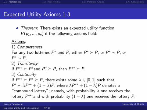
Expected Utility Axioms 1-3
Theorem: There exists an expected utility functionV (p1; :::; pn) if the following axioms hold:
Axioms:1) CompletenessFor any two lotteries P� and P, either P� � P, or P� � P, orP� � P.2) TransitivityIf P�� � P�and P� � P, then P�� � P.3) ContinuityIf P�� � P� � P, there exists some � 2 [0; 1] such thatP� � �P�� + (1� �)P, where �P�� + (1� �)P denotes a�compound lottery�; namely, with probability � one receives thelottery P�� and with probability (1� �) one receives the lottery P.
George Pennacchi University of Illinois
Expected utility and risk aversion 9/ 58

1.1: Preferences 1.2: Risk Premia 1.3: Portfolio Choice 1.4: Conclusions
Expected Utility Axioms 4-5
4) IndependenceFor any two lotteries P and P�, P� � P if and only if for all � 2(0,1] and all P��:
�P� + (1� �)P�� � �P + (1� �)P��
Moreover, for any two lotteries P and Py, P � Py if and only if forall � 2(0,1] and all P��:
�P + (1� �)P�� � �Py + (1� �)P��
5) DominanceLet P1 be the compound lottery �1Pz + (1� �1)Py and P2 be thecompound lottery �2Pz + (1� �2)Py. If Pz � Py, then P1 � P2 ifand only if �1 > �2.
George Pennacchi University of Illinois
Expected utility and risk aversion 10/ 58

1.1: Preferences 1.2: Risk Premia 1.3: Portfolio Choice 1.4: Conclusions
Discussion: Machina (1987)
The �rst three axioms are analogous to those used to establisha real-valued utility function in consumer choice theory.
Axiom 4 (Independence) is novel, but its linearity property iscritical for preferences to be consistent with expected utility.
To understand its meaning, suppose an individual chooses P�
� P. By Axiom 4, the choice between �P� + (1� �)P�� and�P + (1� �)P�� is equivalent to tossing a coin that withprobability (1� �) lands �tails,� in which both lotteries payP��, and with probability � lands �heads,� in which case theindividual should prefer P� to P.
George Pennacchi University of Illinois
Expected utility and risk aversion 11/ 58

1.1: Preferences 1.2: Risk Premia 1.3: Portfolio Choice 1.4: Conclusions
Allais Paradox
But, there is some experimental evidence counter to thisaxiom.
Consider lotteries over fx1; x2; x3g = f$0; $1m; $5mg and twolottery choices:C1: P1 = f0; 1; 0g vs P2 = f:01; :89; :1gC2: P3 = f:9; 0; :1g vs P4 = f:89; :11; 0g
Which do you choose in C1? In C2?
George Pennacchi University of Illinois
Expected utility and risk aversion 12/ 58

1.1: Preferences 1.2: Risk Premia 1.3: Portfolio Choice 1.4: Conclusions
Allais Paradox
Experimental evidence suggests most people prefer P1 � P2and P3 � P4.
But this violates Axiom 4. Why?
De�ne P5 = f1=11; 0; 10=11g and let � = 0:11. Note that P2is equivalent to the compound lottery:
P2 � �P5 + (1� �)P1
� 0:11f1=11; 0; 10=11g+ 0:89f0; 1; 0g� f:01; :89; :1g
George Pennacchi University of Illinois
Expected utility and risk aversion 13/ 58

1.1: Preferences 1.2: Risk Premia 1.3: Portfolio Choice 1.4: Conclusions
Allais Paradox
Note also that P1 is trivially the compound lottery�P1 + (1� �)P1. Hence, if P1 � P2, the independenceaxiom implies P1 � P5.Now also de�ne P6 = f1; 0; 0g, and note that P3 equals thefollowing compound lottery:
P3 � �P5 + (1� �)P6
� 0:11f1=11; 0; 10=11g+ 0:89f1; 0; 0g� f:9; 0; :1g
while P4 is equivalent to the compound lottery
P4 � �P1 + (1� �)P6
� 0:11f0; 1; 0g+ 0:89f1; 0; 0g� f:89; 0:11; 0g
George Pennacchi University of Illinois
Expected utility and risk aversion 14/ 58

1.1: Preferences 1.2: Risk Premia 1.3: Portfolio Choice 1.4: Conclusions
Allais Paradox
But if P3 � P4, the independence axiom implies P5 � P1,which contradicts the choice of P1 � P2 that impliesP1 � P5.
Despite the sometimes contradictory experimental evidence,expected utility is still the dominant paradigm.
However, we will consider di¤erent models of utility at a laterdate, including those that re�ect psychological biases.
George Pennacchi University of Illinois
Expected utility and risk aversion 15/ 58

1.1: Preferences 1.2: Risk Premia 1.3: Portfolio Choice 1.4: Conclusions
Deriving Expected Utility: Axiom 1
We now prove the theorem by showing that if an individual�spreferences over lotteries satisfy the preceding axioms, thesepreferences can be ranked by the individual�s expected utilityof the lotteries.
De�ne an �elementary�or �primitive� lottery, ei , whichreturns outcome xi with probability 1 and all other outcomeswith probability zero, that is, ei = fp1; :::pi�1;pi ;pi+1:::;png =f0; :::0; 1; 0; :::0g where pi = 1 and pj = 0 8j 6= i .
Without loss of generality, assume that the outcomes areordered such that en � en�1 � ::: � e1. This follows from thecompleteness axiom for this case of n elementary lotteries
George Pennacchi University of Illinois
Expected utility and risk aversion 16/ 58

1.1: Preferences 1.2: Risk Premia 1.3: Portfolio Choice 1.4: Conclusions
Deriving Expected Utility: Axiom 3, Axiom 4
From the continuity axiom, for each ei , there exists aUi 2 [0; 1] such that
ei � Uien + (1� Ui )e1 (2)
and for i = 1, this implies U1 = 0 and for i = n, this impliesUn = 1.
Now a given arbitrary lottery, P = fp1; :::; png, can be viewedas a compound lottery over the n elementary lotteries, whereelementary lottery ei is obtained with probability pi .
P � p1e1 + :::+ pnen
George Pennacchi University of Illinois
Expected utility and risk aversion 17/ 58

1.1: Preferences 1.2: Risk Premia 1.3: Portfolio Choice 1.4: Conclusions
Deriving Expected Utility: Axiom 4
By the independence axiom, and equation (2), the individualis indi¤erent between lottery, P, and the following lottery:
p1e1 + :::+ pnen � p1e1 + :::+ pi�1ei�1 + pi [Uien + (1� Ui )e1]+pi+1ei+1 + :::+ pnen (3)
where the indi¤erence relation in equation (2) substitutes forei on the right-hand side of (3).
By repeating this substitution for all i , i = 1; :::; n, theindividual will be indi¤erent between P and
p1e1 + :::+ pnen �
nXi=1
piUi
!en +
1�
nXi=1
piUi
!e1 (4)
George Pennacchi University of Illinois
Expected utility and risk aversion 18/ 58

1.1: Preferences 1.2: Risk Premia 1.3: Portfolio Choice 1.4: Conclusions
Deriving Expected Utility: Axiom 5
Now de�ne � �nPi=1
piUi . Thus, P � �en + (1� �)e1
Similarly, we can show that any other arbitrary lottery
P� = fp�1 ; :::; p�ng � ��en + (1� ��)e1, where �� �nPi=1
p�i Ui .
We know from the dominance axiom that P� � P i¤ �� > �,implying
nPi=1p�i Ui >
nPi=1piUi .
So we can de�ne the function
V (p1; :::; pn) =nXi=1
piUi (5)
which implies that P� � P i¤ V (p�1 ; :::; p�n) > V (p1; :::; pn).
George Pennacchi University of Illinois
Expected utility and risk aversion 19/ 58

1.1: Preferences 1.2: Risk Premia 1.3: Portfolio Choice 1.4: Conclusions
Deriving Expected Utility: The End
The function in (5) is known as von Neumann-Morgensternexpected utility. It is linear in the probabilities and is uniqueup to a linear monotonic transformation.
The intuition for why expected utility is unique up to a lineartransformation comes from equation (2). Here we expresselementary lottery i in terms of the least and most preferredelementary lotteries. However, other bases for ranking a givenlottery are possible.
For Ui = U(xi ), an individual�s choice over lotteries is thesame under the transformation aU(xi ) + b, but not anonlinear transformation that changes the �shape�of U(xi ).
George Pennacchi University of Illinois
Expected utility and risk aversion 20/ 58

1.1: Preferences 1.2: Risk Premia 1.3: Portfolio Choice 1.4: Conclusions
St. Petersburg Paradox Revisited
Suppose Ui = U(xi ) =pxi . Then the expected utility of the
St. Petersburg payo¤ is
V =nXi=1
piUi =1Xi=1
12ip2i�1 =
1Xi=1
2�12 (i+1) =
1Xi=2
2�i2
= 2�22 + 2�
32 + :::
=1Xi=0
�1p2
�i� 1� 1p
2=
11� 1p
2
� 1� 1p2
=1
2�p2�= 1:707
A certain payment of 1:7072 �= 2:914 ducats has the sameexpected utility as playing the St. Petersburg game.
George Pennacchi University of Illinois
Expected utility and risk aversion 21/ 58

1.1: Preferences 1.2: Risk Premia 1.3: Portfolio Choice 1.4: Conclusions
Super St. Petersburg
The St. Petersburg game has in�nite expected payo¤ becausethe probability of winning declines at rate 2i , while thewinning payo¤ increases at rate 2i .In a �super�St. Petersburg paradox, we can make thewinning payo¤ increase at a rate xi = U�1(2i�1) to causeexpected utility to increase at 2i . For square-root utility,xi = (2i2)2 = 22i�2; that is, x1 = 1, x2 = 4, x3 = 16, and soon. The expected utility of �super�St. Petersburg is
V =nXi=1
piUi =1Xi=1
12ip22i�2 =
1Xi=1
12i2i�1 =1 (6)
Should we be concerned that if prizes grow quickly enough,we can get in�nite expected utility (and valuations) for anychosen form of expected utility function?
George Pennacchi University of Illinois
Expected utility and risk aversion 22/ 58

1.1: Preferences 1.2: Risk Premia 1.3: Portfolio Choice 1.4: Conclusions
Von Neumann-Morgenstern Utility
The von Neumann-Morgenstern expected utility can begeneralized to a continuum of outcomes and lotteries withcontinuous probability distributions. Analogous to equation(5) is
V (F ) = E [U (ex)] = Z U (x) dF (x) =ZU (x) f (x) dx (7)
where F (x) is the lottery�s cumulative distribution functionover the payo¤s, x . V can be written in terms of theprobability density, f (x), when F (x) is absolutely continuous.
This is analogous to our previous lottery represented by thediscrete probabilities P = fp1; :::; png.
George Pennacchi University of Illinois
Expected utility and risk aversion 23/ 58

1.1: Preferences 1.2: Risk Premia 1.3: Portfolio Choice 1.4: Conclusions
Risk Aversion
Diminishing marginal utility results in risk aversion: beingunwilling to accept a �fair� lottery. Why?Let there be a lottery that has a random payo¤, e", where
e" = � "1with probability p"2 with probability 1� p
(8)
The requirement that it be a �fair� lottery restricts itsexpected value to equal zero:
E [e"] = p"1 + (1� p)"2 = 0 (9)
which implies "1="2 = � (1� p) =p, or solving for p,p = �"2= ("1 � "2). Since 0 < p < 1, "1 and "2 are ofopposite signs.
George Pennacchi University of Illinois
Expected utility and risk aversion 24/ 58

1.1: Preferences 1.2: Risk Premia 1.3: Portfolio Choice 1.4: Conclusions
Risk Aversion and Concave Utility
Suppose a vN-M maximizer with current wealth W is o¤ereda fair lottery. Would he accept it?With the lottery, expected utility is E [U (W + e")]. Withoutit, expected utility is E [U (W )] = U (W ). Rejecting it implies
U (W ) > E [U (W + e")] = pU (W + "1)+ (1� p)U (W + "2)(10)
U (W ) can be written as
U(W ) = U (W + p"1 + (1� p)"2) (11)
Substituting into (10), we have
U (W + p"1 + (1� p)"2) > pU (W + "1)+(1�p)U (W + "2)(12)
which is the de�nition of U being a concave function.
George Pennacchi University of Illinois
Expected utility and risk aversion 25/ 58

1.1: Preferences 1.2: Risk Premia 1.3: Portfolio Choice 1.4: Conclusions
Risk Aversion , Concavity
A function is concave if a line joining any two points liesentirely below the function. When U(W ) is a continuous,second di¤erentiable function, concavity implies U 00(W ) < 0.
George Pennacchi University of Illinois
Expected utility and risk aversion 26/ 58

1.1: Preferences 1.2: Risk Premia 1.3: Portfolio Choice 1.4: Conclusions
Risk Aversion , Concavity
To show that concave utility implies rejecting a fair lottery, wecan use Jensen�s inequality which says that for concave U(�)
E [U(~x)] < U(E [~x ]) (13)
Therefore, substituting ~x =W + e" with E [e"] = 0, we haveE [U(W + e")] < U (E [W + e"]) = U(W ) (14)
which is the desired result.
George Pennacchi University of Illinois
Expected utility and risk aversion 27/ 58

1.1: Preferences 1.2: Risk Premia 1.3: Portfolio Choice 1.4: Conclusions
Risk Aversion and Risk Premium
How might aversion to risk be quanti�ed? One way is tode�ne a risk premium as the amount that an individual iswilling to pay to avoid a risk.Let � denote the individual�s risk premium for a lottery, e". �is the maximum insurance payment an individual would pay toavoid the lottery risk:
U(W � �) = E [U(W + e")] (15)
W � � is de�ned as the certainty equivalent level of wealthassociated with the lottery, e".For concave utility, Jensen�s inequality implies � > 0 when e" isfair: the individual would accept wealth lower than herexpected wealth following the lottery, E [W + e"], to avoid thelottery.
George Pennacchi University of Illinois
Expected utility and risk aversion 28/ 58

1.1: Preferences 1.2: Risk Premia 1.3: Portfolio Choice 1.4: Conclusions
Risk Premium
For small e" we can take a Taylor approximation of equation(15) around e" = 0 and � = 0.Expanding the left-hand side about � = 0 gives
U(W � �) �= U(W )� �U 0(W ) (16)
and expanding the right-hand side about e" givesE [U(W + e")] �= E �U(W ) + e"U 0(W ) + 1
2e"2U 00(W )� (17)
= U(W ) + 0+ 12�
2U 00(W )
where �2 � E�e"2� is the lottery�s variance.
George Pennacchi University of Illinois
Expected utility and risk aversion 29/ 58

1.1: Preferences 1.2: Risk Premia 1.3: Portfolio Choice 1.4: Conclusions
Risk Premium cont�d
Equating the results in (16) and (17) gives
� = �12�
2U00(W )U 0(W )
� 12�
2R(W ) (18)
where R(W ) � �U 00(W )=U 0(W ) is the Pratt (1964)-Arrow(1971) measure of absolute risk aversion.
Since �2 > 0, U 0(W ) > 0, and U 00(W ) < 0, concavity of theutility function ensures that � must be positive
An individual may be very risk averse (�U 00(W ) is large), butmay be unwilling to pay a large risk premium if he is poorsince his marginal utility U 0(W ) is high.
George Pennacchi University of Illinois
Expected utility and risk aversion 30/ 58
1.1: Preferences 1.2: Risk Premia 1.3: Portfolio Choice 1.4: Conclusions
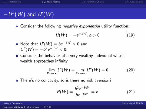
�U 00(W ) and U 0(W )
Consider the following negative exponential utility function:
U(W ) = �e�bW ; b > 0 (19)
Note that U 0(W ) = be�bW > 0 andU 00(W ) = �b2e�bW < 0.Consider the behavior of a very wealthy individual whosewealth approaches in�nity
limW!1
U 0(W ) = limW!1
U 00(W ) = 0 (20)
There�s no concavity, so is there no risk aversion?
R(W ) =b2e�bW
be�bW= b (21)
George Pennacchi University of Illinois
Expected utility and risk aversion 31/ 58

1.1: Preferences 1.2: Risk Premia 1.3: Portfolio Choice 1.4: Conclusions
Absolute Risk Aversion: Dollar Payment for Risk
We see that negative exponential utility, U(W ) = �e�bW ,has constant absolute risk aversion.
If, instead, we want absolute risk aversion to decline in wealth,a necessary condition is that the utility function must have apositive third derivative:
@R(W )@W
=@ � U 00(W )
U 0(W )
@W= �U
000(W )U 0(W )� [U 00(W )]2[U 0(W )]2
(22)
George Pennacchi University of Illinois
Expected utility and risk aversion 32/ 58

1.1: Preferences 1.2: Risk Premia 1.3: Portfolio Choice 1.4: Conclusions
R(W )) U(W )
The coe¢ cient of risk aversion contains all relevantinformation about the individual�s risk preferences. Note that
R(W ) = �U00(W )U 0(W )
= �@ (ln [U0(W )])
@W(23)
Integrating both sides of (23), we have
�ZR(W )dW = ln[U 0(W )] + c1 (24)
where c1 is an arbitrary constant. Taking the exponentialfunction of (24) gives
e�RR(W )dW = U 0(W )ec1 (25)
George Pennacchi University of Illinois
Expected utility and risk aversion 33/ 58

1.1: Preferences 1.2: Risk Premia 1.3: Portfolio Choice 1.4: Conclusions
R(W )) U(W ) cont�d
Integrating once again, we obtainZe�
RR(W )dW dW = ec1U(W ) + c2 (26)
where c2 is another arbitrary constant.
Because vN-M expected utility functions are unique up to alinear transformation, ec1U(W ) + c2 re�ects the same riskpreferences as U(W ).
George Pennacchi University of Illinois
Expected utility and risk aversion 34/ 58

1.1: Preferences 1.2: Risk Premia 1.3: Portfolio Choice 1.4: Conclusions
Relative Risk Aversion
Relative risk aversion is another frequently used measurede�ned as
Rr (W ) =WR(W ) (27)
Consider risk aversion for some utility functions often used inmodels of portfolio choice and asset pricing. Power utility canbe written as
U(W ) = 1 W
; < 1 (28)
implying that R(W ) = � ( �1)W �2
W �1 = (1� )W and, therefore,
Rr (W ) = 1� .Hence, it displays constant relative risk aversion.
George Pennacchi University of Illinois
Expected utility and risk aversion 35/ 58

1.1: Preferences 1.2: Risk Premia 1.3: Portfolio Choice 1.4: Conclusions
Logarithmic Utility: Constant Relative Risk Aversion
Logarithmic utility is a limiting case of power utility. Sinceutility functions are unique up to a linear transformation, writethe power utility function as
1 W
� 1 =W � 1
Next take its limit as ! 0. Do so by rewriting thenumerator and applying L�Hôpital�s rule:
lim !0
W � 1
= lim !0
e ln(W ) � 1
= lim !0
ln(W )W
1= ln(W )
(29)Thus, logarithmic utility is power utility with coe¢ cient ofrelative risk aversion (1� ) = 1 since R(W ) = �W �2
W �1 =1W
and Rr (W ) = 1.
George Pennacchi University of Illinois
Expected utility and risk aversion 36/ 58

1.1: Preferences 1.2: Risk Premia 1.3: Portfolio Choice 1.4: Conclusions
HARA: Power, Log, Quadratic
Hyperbolic absolute-risk-aversion (HARA) utility generalizesall of the previous utility functions:
U(W ) =1�
��W1� + �
� (30)
s:t: 6= 1, � > 0, �W1� + � > 0, and � = 1 if = �1.
Thus, R(W ) =�W1� +
��
��1. Since R(W ) must be > 0, it
implies � > 0 when > 1. Rr (W ) =W�W1� +
��
��1.
HARA utility nests constant absolute risk aversion ( = �1,� = 1), constant relative risk aversion ( < 1, � = 0), andquadratic ( = 2) utility functions.
George Pennacchi University of Illinois
Expected utility and risk aversion 37/ 58

1.1: Preferences 1.2: Risk Premia 1.3: Portfolio Choice 1.4: Conclusions
Another Look at the Risk Premium
A premium to avoid risk is �ne for insurance, but we may alsobe interested in a premium to bear risk.
This alternative concept of a risk premium was used by Arrow(1971), identical to the earlier one by Pratt (1964).
Suppose that a fair lottery e", has the following payo¤s andprobabilities:
e" = � +� with probability 12
�� with probability 12
(31)
How much do we need to deviate from �fairness� to make arisk-averse individual indi¤erent to this lottery?
George Pennacchi University of Illinois
Expected utility and risk aversion 38/ 58

1.1: Preferences 1.2: Risk Premia 1.3: Portfolio Choice 1.4: Conclusions
Risk Premium v2
Let�s de�ne a risk premium, �, in terms of probability ofwinning p:
� = Prob(win)� Prob(lose) = p � (1� p) = 2p � 1 (32)
Therefore, from (32) we have
Prob(win) � p = 12 (1+ �)
Prob(lose) = 1� p = 12 (1� �)
We want � that equalizes the utilities of taking and not takingthe lottery:
U(W ) =12(1+ �)U(W + �) +
12(1� �)U(W � �) (33)
George Pennacchi University of Illinois
Expected utility and risk aversion 39/ 58

1.1: Preferences 1.2: Risk Premia 1.3: Portfolio Choice 1.4: Conclusions
Risk Aversion (again)
Let�s again take a Taylor approximation of the right side,around � = 0
U(W ) =12(1+ �)
�U(W ) + �U 0(W ) + 1
2 �2U 00(W )
�(34)
+12(1� �)
�U(W )� �U 0(W ) + 1
2 �2U 00(W )
�= U(W ) + ��U 0(W ) + 1
2 �2U 00(W )
Rearranging (34) implies
� = 12 �R(W ) (35)
which, as before, is a function of the coe¢ cient of absoluterisk aversion.
George Pennacchi University of Illinois
Expected utility and risk aversion 40/ 58

1.1: Preferences 1.2: Risk Premia 1.3: Portfolio Choice 1.4: Conclusions
Risk Aversion (again)
Note that the Arrow premium, �, is in terms of a probability,while the Pratt measure, �, is in units of a monetary payment.
If we multiply � by the monetary payment received, �, thenequation (35) becomes
�� = 12 �2R(W ) (36)
Since �2 is the variance of the random payo¤, e", equation (36)shows that the Pratt and Arrow risk premia are equivalent.Both were obtained as a linearization of the true functionaround e" = 0.
George Pennacchi University of Illinois
Expected utility and risk aversion 41/ 58

1.1: Preferences 1.2: Risk Premia 1.3: Portfolio Choice 1.4: Conclusions
A Simple Portfolio Choice Problem
Let�s consider the relation between risk aversion and anindividual�s portfolio choice in a single period context.Assume there is a riskless security that pays a rate of returnequal to rf and just one risky security that pays a stochasticrate of return equal to er .Also, let W0 be the individual�s initial wealth, and let A be thedollar amount that the individual invests in the risky asset atthe beginning of the period. Thus, W0 � A is the initialinvestment in the riskless security.Denote the individual�s end-of-period wealth as ~W :
~W = (W0 � A)(1+ rf ) + A(1+ ~r) (37)
= W0(1+ rf ) + A(~r � rf )
George Pennacchi University of Illinois
Expected utility and risk aversion 42/ 58

1.1: Preferences 1.2: Risk Premia 1.3: Portfolio Choice 1.4: Conclusions
Single Period Utility Maximization
A vN-M expected utility maximizer chooses her portfolio bymaximizing the expected utility of end-of-period wealth:
maxAE [U( ~W )] = max
AE [U (W0(1+ rf ) + A(~r � rf ))] (38)
Maximization satis�es the �rst-order condition wrt. A:
EhU 0�~W�(~r � rf )
i= 0 (39)
Note that the second order condition
EhU 00�~W�(~r � rf )2
i� 0 (40)
is satis�ed because U 00�~W�� 0 from concavity.
George Pennacchi University of Illinois
Expected utility and risk aversion 43/ 58

1.1: Preferences 1.2: Risk Premia 1.3: Portfolio Choice 1.4: Conclusions
Obtaining A� from FOC
If E [~r � rf ] = 0, i.e., E [~r ] = rf , then we can show A=0 is thesolution.
When A=0, ~W =W0 (1+ rf ) and, therefore,
U 0�~W�= U 0 (W0 (1+ rf )) is nonstochastic. Hence,
EhU 0�~W�(~r � rf )
i= U 0 (W0 (1+ rf ))E [~r � rf ] = 0.
Next, suppose E [~r � rf ] > 0.A = 0 is not a solution becauseEhU 0�~W�(~r � rf )
i= U 0 (W0 (1+ rf ))E [~r � rf ] > 0 when
A = 0.
Thus, when E [~r ]� rf > 0, let�s show that A > 0.
George Pennacchi University of Illinois
Expected utility and risk aversion 44/ 58

1.1: Preferences 1.2: Risk Premia 1.3: Portfolio Choice 1.4: Conclusions
Why must A > 0?
Let rh denote a realization of ~r > rf , and let W h be thecorresponding level of ~W
Also, let r l denote a realization of ~r < rf , and let W l be thecorresponding level of ~W .
Then U 0(W h)(rh � rf ) > 0 and U 0(W l )(r l � rf ) < 0.
For U 0�~W�(~r � rf ) to average to zero for all realizations of
~r , it must be that W h >W l so that U 0�W h�< U 0
�W l�due
to the concavity of the utility function.
Why? Since E [~r ]� rf > 0, the average rh is farther above rfthan the average r l is below rf . To preserve (39), themultipliers must satisfy U 0
�W h�< U 0
�W l�to compensate,
which occurs when W h >W l and which requires that A > 0.
George Pennacchi University of Illinois
Expected utility and risk aversion 45/ 58
1.1: Preferences 1.2: Risk Premia 1.3: Portfolio Choice 1.4: Conclusions
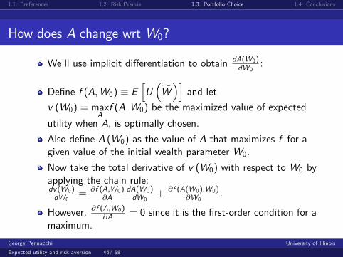
How does A change wrt W0?
We�ll use implicit di¤erentiation to obtain dA(W0)dW0
:
De�ne f (A;W0) � EhU�fW�i and let
v (W0) = maxAf (A;W0) be the maximized value of expected
utility when A, is optimally chosen.
Also de�ne A (W0) as the value of A that maximizes f for agiven value of the initial wealth parameter W0.
Now take the total derivative of v (W0) with respect to W0 byapplying the chain rule:dv (W0)dW0
= @f (A;W0)@A
dA(W0)dW0
+ @f (A(W0);W0)@W0
.
However, @f (A;W0)@A = 0 since it is the �rst-order condition for a
maximum.
George Pennacchi University of Illinois
Expected utility and risk aversion 46/ 58

1.1: Preferences 1.2: Risk Premia 1.3: Portfolio Choice 1.4: Conclusions
How does A change wrt W0 cont�d
The total derivative simpli�es to dv (W0)dW0
= @f (A(W0);W0)@W0
:
Thus, the derivative of the maximized value of the objectivefunction with respect to a parameter is just the partialderivative with respect to that parameter.
Second, consider how the optimal value of the controlvariable, A (W0), changes when the parameter W0 changes.
Derive this relationship by taking the total derivative of theF.O.C. (39), @f (A (W0) ;W0) =@A = 0, with respect to W0:
@(@f (A(W0);W0)=@A)@W0
= 0 =@2f (A(W0);W0)@A2
dA(W0)dW0
+@2f (A(W0);W0)@A@W0
George Pennacchi University of Illinois
Expected utility and risk aversion 47/ 58

1.1: Preferences 1.2: Risk Premia 1.3: Portfolio Choice 1.4: Conclusions
How does A change wrt W0 cont�d
Rearranging the above gives us
dA (W0)
dW0= �@
2f (A (W0) ;W0)
@A@W0=@2f (A (W0) ;W0)
@A2(41)
We can then evaluate it to obtain
dAdW0
=(1+ rf )E
hU 00( ~W )(~r � rf )
i�E
hU 00( ~W )(~r � rf )2
i (42)
The denominator of (42) is positive because of concavity.Therefore, the sign of dA
dW0depends on the numerator.
George Pennacchi University of Illinois
Expected utility and risk aversion 48/ 58

1.1: Preferences 1.2: Risk Premia 1.3: Portfolio Choice 1.4: Conclusions
Implications for dAdW0
with DARA
Consider an individual with absolute risk aversion that isdecreasing in wealth. Assuming E [~r ] > rf so that A > 0:
R�W h�< R (W0(1+ rf )) (43)
where, as before, R(W ) = �U 00(W )=U 0(W ).Multiplying both terms of (43) by �U 0(W h)(rh � rf ), which isa negative quantity, the inequality sign changes:
U 00(W h)(rh � rf ) > �U 0(W h)(rh � rf )R (W0(1+ rf )) (44)
Then for A > 0, we have W l <W0(1+ rf ). If absolute riskaversion is decreasing in wealth, this implies
R(W l ) > R (W0(1+ rf )) (45)
George Pennacchi University of Illinois
Expected utility and risk aversion 49/ 58

1.1: Preferences 1.2: Risk Premia 1.3: Portfolio Choice 1.4: Conclusions
Implications for dAdW0
with DARA
Multiplying (45) by �U 0(W l )(r l � rf ), which is positive, sothat the sign of (45) remains the same, we obtain
U 00(W l )(r l � rf ) > �U 0(W l )(r l � rf )R (W0(1+ rf )) (46)
Inequalities (44) and (46) are the same whether therealization is ~r = rh or ~r = r l .
Therefore, if we take expectations over all realizations of ~r , weobtain
EhU 00( ~W )(~r � rf )
i> �E
hU 0( ~W )(~r � rf )
iR (W0(1+ rf ))
(47)
The �rst term on the right-hand side is just the FOC.
George Pennacchi University of Illinois
Expected utility and risk aversion 50/ 58

1.1: Preferences 1.2: Risk Premia 1.3: Portfolio Choice 1.4: Conclusions
Implications for risk-taking with ARA/RRA
Inequality (47) reduces to
EhU 00( ~W )(~r � rf )
i> 0 (48)
Thus, DARA ) dA=dW0 > 0: amount invested A increases ininitial wealth.What about the proportion of initial wealth? To analyze this,de�ne
� �dAdW0AW0
=dAdW0
W0
A(49)
which is the elasticity measuring the proportional increase inthe risky asset for an increase in initial wealth.
George Pennacchi University of Illinois
Expected utility and risk aversion 51/ 58

1.1: Preferences 1.2: Risk Premia 1.3: Portfolio Choice 1.4: Conclusions
Implications for risk-taking with RRA
Adding 1� AA to the right-hand side of (49) gives
� = 1+(dA=dW0)W0 � A
A(50)
Substituting dA=dW0 from equation (42), we have
� = 1+W0(1+ rf )E
hU 00( ~W )(~r � rf )
i+ AE
hU 00( ~W )(~r � rf )2
i�AE
hU 00( ~W )(~r � rf )2
i(51)
Collecting terms in U 00( ~W )(~r � rf ), this can be rewritten as
George Pennacchi University of Illinois
Expected utility and risk aversion 52/ 58

1.1: Preferences 1.2: Risk Premia 1.3: Portfolio Choice 1.4: Conclusions
Implications for risk-taking with RRA
� = 1+EhU 00( ~W )(~r � rf )fW0(1+ rf ) + A(~r � rf )g
i�AE
hU 00( ~W )(~r � rf )2
i (52)
= 1+EhU 00( ~W )(~r � rf ) ~W
i�AE
hU 00( ~W )(~r � rf )2
i (53)
The denominator in (53) is positive for A > 0 by concavity.Therefore, � > 1, so that the individual invests proportionallymore in the risky asset with an increase in wealth, ifEhU 00( ~W )(~r � rf ) ~W
i> 0.
Can we relate this to the individual�s risk aversion?George Pennacchi University of Illinois
Expected utility and risk aversion 53/ 58

1.1: Preferences 1.2: Risk Premia 1.3: Portfolio Choice 1.4: Conclusions
Implications for risk-taking with DRRA
Consider an individual whose relative risk aversion isdecreasing in wealth.
Then for A > 0, we again have W h >W0(1+ rf ). WhenRr (W ) �WR(W ) is decreasing in wealth, this implies
W hR(W h) <W0(1+ rf )R (W0(1+ rf )) (54)
Multiplying both terms of (54) by �U 0(W h)(rh � rf ), which isa negative quantity, the inequality sign changes:
W hU 00(W h)(rh�rf ) > �U 0(W h)(rh�rf )W0(1+rf )R (W0(1+ rf ))(55)
George Pennacchi University of Illinois
Expected utility and risk aversion 54/ 58

1.1: Preferences 1.2: Risk Premia 1.3: Portfolio Choice 1.4: Conclusions
Implications for risk-taking with DRRA
For A > 0, we have W l <W0(1+ rf ). If relative risk aversionis decreasing in wealth, this implies
W lR(W l ) >W0(1+ rf )R (W0(1+ rf )) (56)
Multiplying (56) by �U 0(W l )(r l � rf ), which is positive, sothat the sign of (56) remains the same, we obtain
W lU 00(W l )(r l�rf ) > �U 0(W l )(r l�rf )W0(1+rf )R (W0(1+ rf ))(57)
Inequalities (55) and (57) are the same whether therealization is ~r = rh or ~r = r l .
Therefore, taking expectations over all realizations of ~r yields
George Pennacchi University of Illinois
Expected utility and risk aversion 55/ 58
1.1: Preferences 1.2: Risk Premia 1.3: Portfolio Choice 1.4: Conclusions
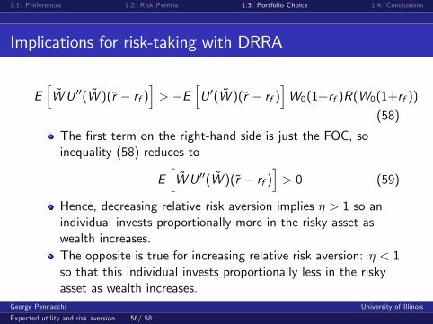
Implications for risk-taking with DRRA
Eh~WU 00( ~W )(~r � rf )
i> �E
hU 0( ~W )(~r � rf )
iW0(1+rf )R(W0(1+rf ))
(58)
The �rst term on the right-hand side is just the FOC, soinequality (58) reduces to
Eh~WU 00( ~W )(~r � rf )
i> 0 (59)
Hence, decreasing relative risk aversion implies � > 1 so anindividual invests proportionally more in the risky asset aswealth increases.The opposite is true for increasing relative risk aversion: � < 1so that this individual invests proportionally less in the riskyasset as wealth increases.
George Pennacchi University of Illinois
Expected utility and risk aversion 56/ 58

1.1: Preferences 1.2: Risk Premia 1.3: Portfolio Choice 1.4: Conclusions
Risk-taking with ARA/RRA
The main results of this section can be summarized as:
Risk Aversion Investment BehaviorDecreasing Absolute @A
@W0> 0
Constant Absolute @A@W0
= 0Increasing Absolute @A
@W0< 0
Decreasing Relative @A@W0
> AW0
Constant Relative @A@W0
= AW0
Increasing Relative @A@W0
< AW0
George Pennacchi University of Illinois
Expected utility and risk aversion 57/ 58

1.1: Preferences 1.2: Risk Premia 1.3: Portfolio Choice 1.4: Conclusions
Conclusions
We have shown:
� Why expected utility, rather than expected value, is a bettercriterion for choosing and valuing assets.
� What conditions preferences can satisfy to be represented byan expected utility function.
� The relationship between a utility function, U(W ), and riskaversion.
� How ARA/RRA a¤ects the choice between risky and risk-freeassets.
George Pennacchi University of Illinois
Expected utility and risk aversion 58/ 58
Related Documents


![Risk-Aversion Concepts in Expected- and Non-Expected ...RISK-AVERSION CONCEPTS 75 The two sets %9 and ~3 are mixtures spaces in the following sense: for any ot of [0, 1], any X and](https://static.cupdf.com/doc/110x72/5feab2526517b14ffa4f6b5f/risk-aversion-concepts-in-expected-and-non-expected-risk-aversion-concepts.jpg)


