Existence and stability analysis of semifluxons in disk-shaped two-dimensional 0-pi Josephson junctions

Existence and stability analysis of semifluxons in disk-shaped two-dimensional0-� Josephson junctions

Saeed Ahmad,1,* Hadi Susanto,1 Jonathan A. D. Wattis,1 and Edward Goldobin2,†

1School of Mathematical Sciences, University of Nottingham, University Park, Nottingham NG7 2RD, United Kingdom2Physikalisches Institut, Experimentalphysik II and Center for Collective Quantum Phenomena, Universität Tübingen,

Auf der Morgenstelle 14, D-72076 Tübingen, Germany�Received 11 August 2010; published 5 November 2010�

We consider a disk-shaped two-dimensional Josephson junction with concentric regions of 0- and �-phaseshifts and investigate its ground states. This system is described by a �2+1�-dimensional sine-Gordon equation,which becomes effectively one dimensional in polar coordinates when one considers radially symmetric staticsolutions. We show that there is a parameter region in which the ground state corresponds to a spontaneouslycreated ring-shaped semifluxon. We use a Hamiltonian energy characterization to describe analytically thedependence of the semifluxonlike ground state on the junction size and the applied bias current. We presentnumerical calculations to support our analytical results. We also discuss the existence and stability of excitedstates bifurcating from a uniform solution.

DOI: 10.1103/PhysRevB.82.174504 PACS number�s�: 74.50.�r, 85.25.Cp, 74.20.Rp

I. INTRODUCTION

Investigation of solitons in long Josephson junctions�LJJs� attracted a lot of attention in the last few decades.1

Mathematically they are topological solitons �kinks� of asine-Gordon model. Physically, if the phase difference of thesuperconductors is denoted by ��x�, a kink in the context ofLJJs corresponds to a vortex of supercurrent proportional tosin ��x�, which creates a localized magnetic field �d� /dxwith a total magnetic flux ��0� �2.07�10−15 Wb, i.e., amagnetic-flux quantum. Traditionally, one investigates themost simple one-dimensional �1D� geometry, i.e., a�1+1�-dimensional sine-Gordon equation, in which only thephase variation in the x direction is considered, while thephase dynamics in the y direction is neglected. This is justi-fied when the width w of the junction in y direction is lessthan or approximately equal to the Josephson length �J. Inthis case, the soliton can be viewed as a uniform flux tubegoing along the short y direction.

If one considers LJJs with both lateral sizes w �along y�and L �along x� �J, then one should use a�2+1�-dimensional sine-Gordon model.2 In such a model,one still can observe solutions in the �1+1�-dimensionalcounterpart. In addition, one can see the shape of wavespropagating along the y direction, especially when a solitonhits obstacles.3,4 Nonetheless, such �2+1�-dimensional soli-tons are still topologically equivalent to a simple flux line.On the other hand, in two spatial dimensions, one may alsoimagine solutions of completely different topology, such as aflux line closed in a loop �ring�. In a uniform system, suchsolitons are unstable5,6—even with initial velocity outward�an expanding soliton ring�, they exhibit a “return effect”7

and collapse into the center, resulting in a “pulson”8,9 andfinally decaying into the trivial constant phase solution.

Over the last decade, nonconventional JJs having a phasedrop of � in the ground state, called � junctions, were dis-covered and investigated experimentally.10–15 In this context,conventional junctions are called 0 junctions. In terms of asine-Gordon model, this means that there is a shift of � in

the phase difference �. All solutions are therefore shifted by� but no new phenomena appear.

Nontrivial properties occur when one combines 0 and �junctions in one device, making the so-called 0-� LJJ. Suchjunctions can be produced by using several technologies.16–18

If the 0 and � parts are long enough, a flux line, i.e., a vortexof supercurrent, is formed along the 0-� boundary and con-stitutes the ground state of the system. Such vortex carriesonly a half of the magnetic-flux quantum, i.e., ��0 /2 and,therefore, is called semifluxon. Semifluxons were predicted19

and observed experimentally.16 Among all 0-� JJtechnologies available nowadays, only superconductor-ferromagnetic-superconductor �SFS� or superconductor-insulator-ferromagnetic-superconductor �SIFS� technologyallows the fabrication of the 0-� boundary of arbitraryshape. Indeed, recently 0-� LJJs with 0-� boundary forminga loop were successfully fabricated and the supercurrenttransport in them was visualized.20

In this paper, we consider theoretically a two-dimensional�2D� disk-shaped Josephson junction, with the inner circular� part and the outer 0 part having, respectively, a radius fromRmin to Rmid and a radius from Rmid to Rmax, as sketched inFig. 1. In particular, we analyze the existence and stability ofdifferent static solutions to find the ground state of the sys-tem.

The paper is organized as follows. In Sec. II, the model isintroduced. In Sec. III, we analyze the stability of uniformsolutions in the case of no applied bias current and show that

FIG. 1. �Color online� A sketch of the disk-shaped two-dimensional 0-� Josephson junction considered in this paper.

PHYSICAL REVIEW B 82, 174504 �2010�

1098-0121/2010/82�17�/174504�15� ©2010 The American Physical Society174504-1

the uniform solutions are unstable in a certain parameter in-terval. In this interval of parameters a semifluxon is sponta-neously created. The existence and stability of nonuniformstatic solitons is discussed in Sec. IV. In Sec. V, we brieflystudy the existence and stability of excited states. Section VIconcludes this work.

II. MATHEMATICAL MODEL

The dynamics of the Josephson phase in a 2D JJ is gov-erned by the following �2+1�D perturbed sine-Gordon equa-tion:

�xx + �yy − �tt = sin�� + � + ��t − � , �1�

where ��x ,y , t� is a Josephson phase, � 0 is a dimension-less damping coefficient, and � is the applied bias currentdensity normalized to the critical current density jc and as-sumed to be constant. Here we consider a disk-shaped 2D JJsketched in Fig. 1. The origin of the coordinate system issituated in the center of the disk while z=0 corresponds tothe Josephson barrier, which is assumed to be infinitesimal.Thus, Eq. �1� should be solved on the domain

Rmin � �x2 + y2 � Rmax.

The function describes the position of an additional � shiftand is given by

= �� Rmin � �x2 + y2 � Rmid,

0 Rmid � �x2 + y2 � Rmax.� �2�

In this paper we consider only the case Rmin=0.Due to the geometry of the problem, it is convenient to

work in polar coordinates. If �r ,� are the polar coordinatescorresponding to the point �x ,y� in the plane, then the aboveEq. �1� can be written as

�rr +1

r�r +

1

r2� − �tt = sin�� + �r�� + ��t − � . �3�

The function �Eq. �2�� can then be rewritten as

�r� = �� 0 � r � a ,

0 a � r � L .� �4�

Here, for simplicity we have defined Rmid=a and Rmax=L. Inspite of phase jump �Eq. �4�� at r=a, the solution ��r� shouldbe continuous at r=a, i.e.,

��a−� = ��a+� , �5a�

�r�a−� = �r�a+� . �5b�

The boundary conditions corresponding to a zero appliedmagnetic field read

�r�L� = 0, �6a�

�r�Rmin� = 0. �6b�

The condition �Eq. �6b�� is only necessary when Rmin�0 andwill not be used below.

Equation �3� subject to the conditions �Eqs. �5a�, �5b�,�6a�, and �6b�� can be derived from the Lagrangian

L = 0

2� 0

L �1

2�t

2 −1

2�r

2 −1

2r2�2 − 1

+ cos�� + �r�� − ���rdrd . �7�

As we are particularly interested in static solutions, exis-tence of the solution will be studied through the time-independent equation

�rr +1

r�r +

1

r2� = sin�� + �r�� − � . �8�

In the case of -independent solutions, Eq. �8� is simplifiedto

�rr +1

r�r = sin�� + �r�� − � . �9�

Let �0�r ,� be a static solution of the governing equationin a polar coordinate �Eq. �3��. To determine the linear sta-bility of the solution, one then needs to perturb it by writing

� = �0 + ��1.

Substituting the equation above into Eq. �3� and retainingonly the linear terms in � yields the linearized equation

�rr +1

r�r +

1

r2���1 = �cos��0 + �r�� + �tt + ��t��1,

�10�

which governs the dynamics of the small perturbation �1.As Eq. �10� is linear, it can be solved using a separation of

variables method. Writing

�1 = e�tV�r,� , �11�

Eq. �10� becomes the eigenvalue problem

Vrr +1

rVr +

1

r2 V = cos��0 + �r��V + EV , �12�

where

E = �2 + �� . �13�

In the case where �0 is independent of the angular variable

, one can introduce V�r ,�→cos�q�V�r�, which actuallycovers all 2�-periodic functions in that can be representedby Fourier series. Then Eq. �12� becomes

Vrr +1

rVr −

q2V

r2 = �E + cos��0 + �r�� V . �14�

The eigenvalues E in this case are functions of q.Since the eigenvalue problem �Eq. �14�� is self-adjoint,

E�R. The function V�r� is subject to the continuity andboundary conditions that follow from Eqs. �5a�, �5b�, �6a�,and �6b�

V�a−� = V�a+� , �15a�

AHMAD et al. PHYSICAL REVIEW B 82, 174504 �2010�

174504-2

Vr�a−� = Vr�a+� , �15b�

and

Vr�L� = 0, �16a�

Vr�Rmin� = 0. �16b�

The condition �Eq. �16b�� is again only necessary whenRmin�0 and is not used below.

From Eq. �13�, we can easily obtain

�� =1

2�− � � ��2 + 4E� . �17�

In the case �=0, we have ��= ��E, i.e., the solution isstable for E�0 and unstable if E�0. For finite ��0,if E�0 then Re�����0, i.e., solution is stable. If E�0,Re��+� 0 and the solution is unstable. Thus, stability onlydepends on the sign of E and not on the value of �. There-fore, without loss of generality, in the following we set �=0, unless stated otherwise.

III. LINEAR STABILITY ANALYSIS OF UNIFORMSOLUTIONS

It can be easily shown that Eq. �9� has two uniform solu-tions �mod 2��

�0 = 0, �18a�

�0 = � , �18b�

when �=0. In the presence of an applied bias current, i.e.,��0, there is no uniform solution.

To study the stability of the uniform solutions, one needsto solve the eigenvalue problem �Eq. �14�� subject to thecontinuity and boundary conditions �Eqs. �15a�, �15b�, �16a�,and �16b��. From our numerical calculations, it appears thatthe critical eigenvalue of the solutions corresponds to q=0�see Appendix A�. Therefore, in our analytical calculationsbelow, we only consider the case q=0.

Due to the finite size of the domain, the eigenvalue prob-lem �Eq. �14�� has only discrete spectra, which, on the basisof the limit L→�, can be categorized into two types: the setof eigenvalues that constitutes the continuous spectrum inthe limit L→�, which for simplicity we denote as the “con-tinuous” spectrum and the set of eigenvalues that comple-ments the continuous spectrum in the infinite domain limit,which we call the “discrete spectrum.”

A. Linear stability of the �0=0 solution

1. Continuous spectrum

Consider the region 0�r�a, where �r�=�. Let V�1��r�denote the solution to the eigenvalue problem �Eq. �14�� inthis region. Then we obtain

Vrr�1� +

1

rVr

�1� − �E − 1�V�1� = 0, �19�

which is a Bessel equation of order zero with the solution

V�1��r� = C1J0��r� + C1�Y0��r� , �20�

where �=�1−E, J0 and Y0 are Bessel functions of first andsecond kinds, respectively.21 The Bessel function of second

kind Y0��r� is unbounded at r=0. In order to obtain abounded solution of Eq. �19�, we take C1

�=0 and are left with

V�1��r� = C1J0��r� . �21�

Let V�2��r� be the solution to the eigenvalue problem �Eq.

�14�� in the outer region a�r�L, where �r�=0. Hence Eq.�14� takes the form

Vrr�2� +

1

rVr

�2� − �E + 1�V�2� = 0. �22�

The bounded solution to this equation, which is an oscillat-ing function of r at L→�, is

V�2� = C2J0��r� + C3Y0��r� , �23�

where �=�−1−E.Thus, the eigenfunctions of the continuous spectrum of

the uniform zero solution are given by

V�r� =�C1J0��r� 0 � r � a ,

C2J0��r� + C3Y0��r� a � r � L .� �24�

Applying the continuity and boundary conditions�Eqs. �15a�, �15b�, and �16a��, we obtain a system of threehomogenous equations of the form A1U=0, whereU= �C1 ,C2 ,C3�T and A1 is the coefficient matrix defined as

A1�E� = � J0��a� − J0��a� − Y0��a�

− J1��a�� + J1��a�� + Y1��a��

0 − J1��L�� − Y1��L��� . �25�

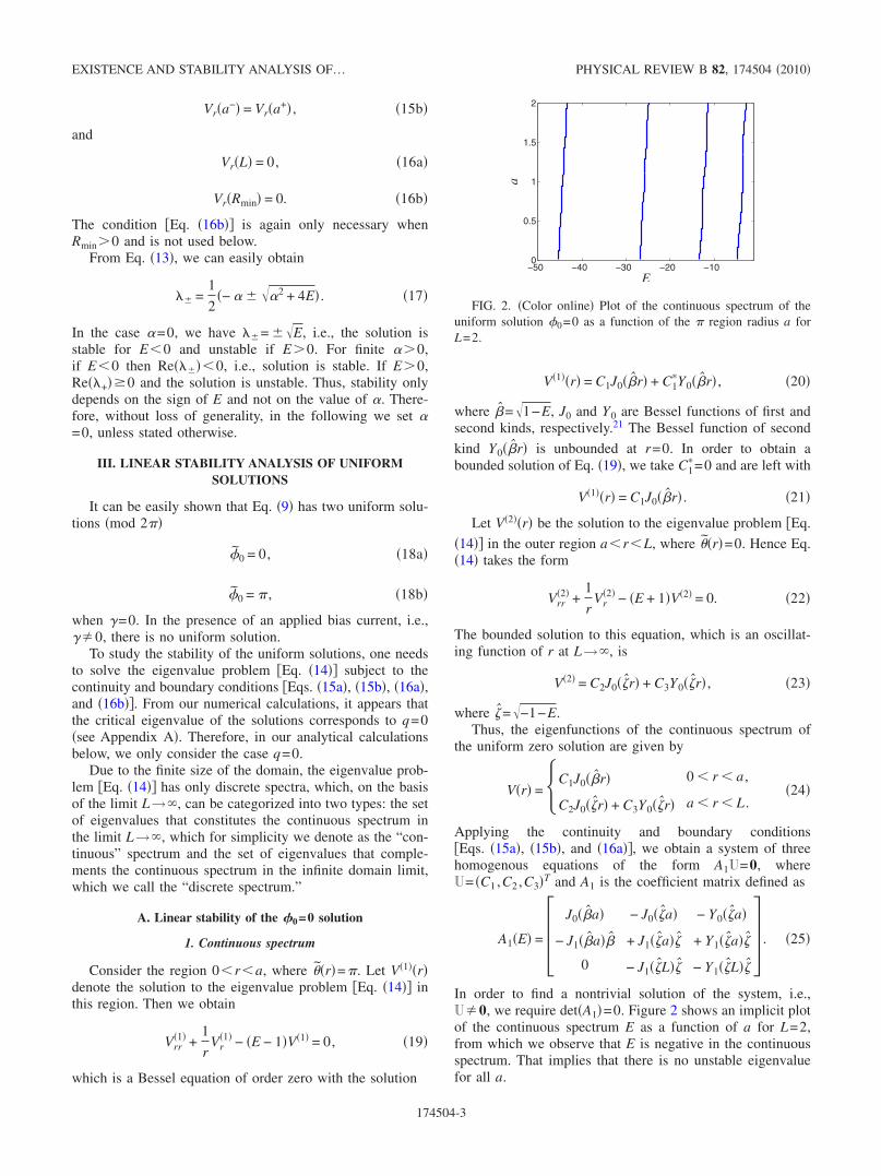
In order to find a nontrivial solution of the system, i.e.,U�0, we require det�A1�=0. Figure 2 shows an implicit plotof the continuous spectrum E as a function of a for L=2,from which we observe that E is negative in the continuousspectrum. That implies that there is no unstable eigenvaluefor all a.

E

a

−50 −40 −30 −20 −100

0.5

1

1.5

2

FIG. 2. �Color online� Plot of the continuous spectrum of theuniform solution �0=0 as a function of the � region radius a forL=2.

EXISTENCE AND STABILITY ANALYSIS OF… PHYSICAL REVIEW B 82, 174504 �2010�

174504-3

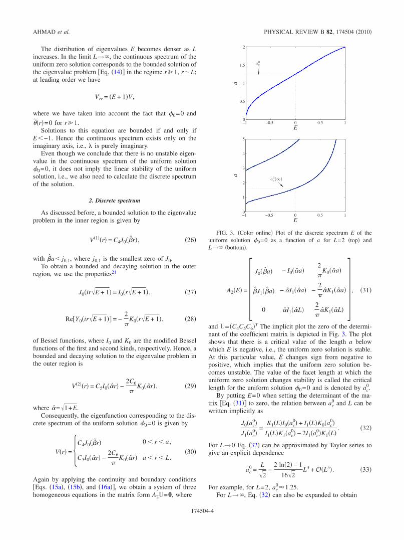
The distribution of eigenvalues E becomes denser as Lincreases. In the limit L→�, the continuous spectrum of theuniform zero solution corresponds to the bounded solution ofthe eigenvalue problem �Eq. �14�� in the regime r�1, r�L;at leading order we have

Vrr = �E + 1�V ,

where we have taken into account the fact that �0=0 and

�r�=0 for r�1.Solutions to this equation are bounded if and only if

E�−1. Hence the continuous spectrum exists only on theimaginary axis, i.e., � is purely imaginary.

Even though we conclude that there is no unstable eigen-value in the continuous spectrum of the uniform solution�0=0, it does not imply the linear stability of the uniformsolution, i.e., we also need to calculate the discrete spectrumof the solution.

2. Discrete spectrum

As discussed before, a bounded solution to the eigenvalueproblem in the inner region is given by

V�1��r� = C4J0��r� , �26�

with �a� j0,1, where j0,1 is the smallest zero of J0.To obtain a bounded and decaying solution in the outer

region, we use the properties21

J0�ir�E + 1� = I0�r�E + 1� , �27�

Re�Y0�ir�E + 1�� = −2

�K0�r�E + 1� , �28�

of Bessel functions, where I0 and K0 are the modified Besselfunctions of the first and second kinds, respectively. Hence, abounded and decaying solution to the eigenvalue problem inthe outer region is

V�2��r� = C5I0��r� −2C6

�K0��r� , �29�

where �=�1+E.Consequently, the eigenfunction corresponding to the dis-

crete spectrum of the uniform solution �0=0 is given by

V�r� = �C4J0��r� 0 � r � a ,

C5I0��r� −2C6

�K0��r� a � r � L .� �30�

Again by applying the continuity and boundary conditions�Eqs. �15a�, �15b�, and �16a��, we obtain a system of threehomogeneous equations in the matrix form A2U=0, where

A2�E� = � J0��a� − I0��a�2

�K0��a�

�J1��a� − �I1��a� −2

��K1��a�

0 �I1��L�2

��K1��L�

� , �31�

and U= �C4C5C6�T The implicit plot the zero of the determi-nant of the coefficient matrix is depicted in Fig. 3. The plotshows that there is a critical value of the length a belowwhich E is negative, i.e., the uniform zero solution is stable.At this particular value, E changes sign from negative topositive, which implies that the uniform zero solution be-comes unstable. The value of the facet length at which theuniform zero solution changes stability is called the criticallength for the uniform solution �0=0 and is denoted by ac

0.By putting E=0 when setting the determinant of the ma-

trix �Eq. �31�� to zero, the relation between ac0 and L can be

written implicitly as

J0�ac0�

J1�ac0�

=K1�L�I0�ac

0� + I1�L�K0�ac0�

I1�L�K1�ac0� − 2I1�ac

0�K1�L�. �32�

For L→0 Eq. �32� can be approximated by Taylor series togive an explicit dependence

ac0 =

L�2

−2 ln�2� − 1

16�2L3 + O�L5� . �33�

For example, for L=2, ac0�1.25.

For L→�, Eq. �32� can also be expanded to obtain

a0c

E

a

−1 −0.5 0 0.5 10

0.5

1

1.5

2

a0c(∞)

E

a

−1 −0.5 0 0.5 10

1

2

3

4

5

FIG. 3. �Color online� Plot of the discrete spectrum E of theuniform solution �0=0 as a function of a for L=2 �top� andL→� �bottom�.

AHMAD et al. PHYSICAL REVIEW B 82, 174504 �2010�

174504-4

�1

L�� 2

�eL�J0�ac

0�K1�ac0� − J1�ac

0�K0�ac0� � = 0. �34�

For the existence of the limit at L→�, we must haveJ0�ac

0�K1�ac0�−J1�ac

0�K0�ac0�=0. Solving for ac

0, we obtain

ac0 � 1.614635. �35�

In this limit, C5→0.The boundary of stability of the �0=0 state given by

ac0�L� is shown in Fig. 4.

B. Linear stability of the �0=� solution

Next, we discuss the linear stability of the uniform solu-tion �0=�.

1. Continuous spectrum

First we consider the inner region 0�r�a where

�r�=�. The eigenvalue problem �Eq. �14�� in this case takesthe form

Vrr +1

rVr − �E + 1�V = 0. �36�

This is a Bessel equation of order 0 whose solution is givenby

V�1��r� = C9J0��r� + C10Y0��r� , �37�

where �=�−1−E.Since Y0 is unbounded at r=0, in order to get a bounded

solution in the inner region we set C10=0 in the above equa-tion. Thus the bounded solution in the inner region is givenby

V�1��r� = C9J0��r� . �38�

For the outer region a�r�L, �r�=0 and Eq. �14� reducesinto the form

Vrr�2� +

1

rVr

�2� − �E − 1�V�2� = 0. �39�

The bounded solution to the Bessel equation �Eq. �39�� is ofthe form

V�2��r� = C11J0��r� + C12Y0��r� , �40�

where C11 and C12 are constants to be determined.Using Eqs. �38� and �40�, the eigenfunctions correspond-

ing to the continuous spectrum of the uniform � solution aredescribed by

V�r� =�C9J0��r� 0 � r � a ,

C11J0��r� + C12Y0��r� a � r � L .� �41�

By using the continuity and boundary conditions, we obtaina homogeneous system of three equations in a matrix formA4U=0, where

A4�E� = � J0��a� − J0��a� − Y0��a�

− J1��a�� J1��a�� Y1��a��

0 − J1��L�� − Y1��L��� �42�

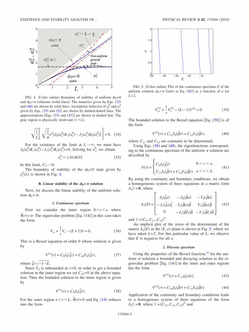
and U= �C9 ,C11,C12�T.An implicit plot of the zeros of the determinant of the

matrix A4�E� in the �E ,a� plane is shown in Fig. 5, where wehave taken L=2. For this particular value of L, we observethat E is negative for all a.

2. Discrete spectrum

Using the properties of the Bessel function,21 for the uni-form � solution a bounded and decaying solution to the ei-genvalue problem �Eq. �14�� in the inner and outer regionshas the form

V�1��r� = C13I0��r� , �43�

V�2��r� = C14J0��r� + C15Y0��r� . �44�

Application of the continuity and boundary conditions leadsto a homogenous system of three equations of the formA5U=0, where U= �C13,C14,C15�T and

FIG. 4. �Color online� Boundary of stability of uniform �0=0and �0=� solutions �solid lines�. The numerics given by Eqs. �32�and �46� are shown by solid lines. Asymptotic behavior of ac

0 and ac�

given by Eqs. �35� and �52� are shown by dashed-dotted lines. Theapproximations �Eqs. �33� and �47�� are shown in dashed line. Thegray region is physically irrelevant �r�L�.

E

a

−50 −40 −30 −20 −100

0.5

1

1.5

2

FIG. 5. �Color online� Plot of the continuous spectrum E of theuniform solution �0=� �refer to Eq. �42�� as a function of a forL=2.

EXISTENCE AND STABILITY ANALYSIS OF… PHYSICAL REVIEW B 82, 174504 �2010�

174504-5

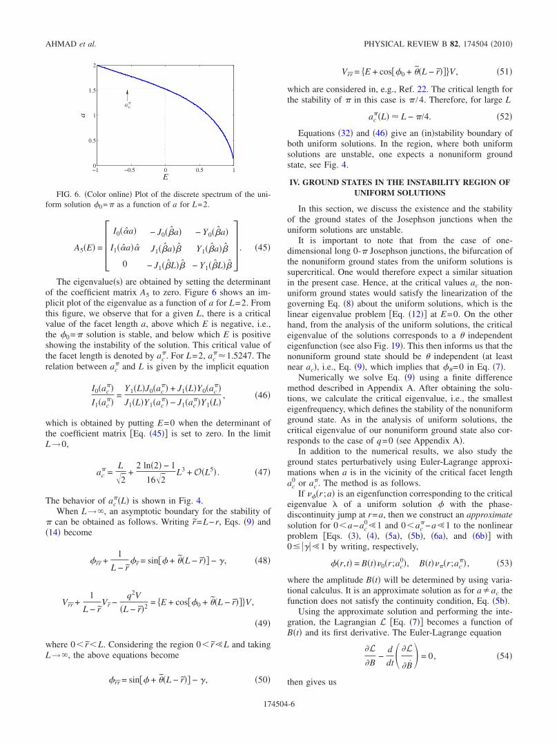
A5�E� = � I0��a� − J0��a� − Y0��a�

I1��a�� J1��a�� Y1��a��

0 − J1��L�� − Y1��L��� . �45�

The eigenvalue�s� are obtained by setting the determinantof the coefficient matrix A5 to zero. Figure 6 shows an im-plicit plot of the eigenvalue as a function of a for L=2. Fromthis figure, we observe that for a given L, there is a criticalvalue of the facet length a, above which E is negative, i.e.,the �0=� solution is stable, and below which E is positiveshowing the instability of the solution. This critical value ofthe facet length is denoted by ac

�. For L=2, ac��1.5247. The

relation between ac� and L is given by the implicit equation

I0�ac��

I1�ac��

=Y1�L�J0�ac

�� + J1�L�Y0�ac��

J1�L�Y1�ac�� − J1�ac

��Y1�L�, �46�

which is obtained by putting E=0 when the determinant ofthe coefficient matrix �Eq. �45�� is set to zero. In the limitL→0,

ac� =

L�2

+2 ln�2� − 1

16�2L3 + O�L5� . �47�

The behavior of ac��L� is shown in Fig. 4.

When L→�, an asymptotic boundary for the stability of� can be obtained as follows. Writing r=L−r, Eqs. �9� and�14� become

�rr +1

L − r�r = sin�� + �L − r�� − � , �48�

Vrr +1

L − rVr −

q2V

�L − r�2 = �E + cos��0 + �L − r�� V ,

�49�

where 0� r�L. Considering the region 0� r�L and takingL→�, the above equations become

�rr = sin�� + �L − r�� − � , �50�

Vrr = �E + cos��0 + �L − r�� V , �51�

which are considered in, e.g., Ref. 22. The critical length forthe stability of � in this case is � /4. Therefore, for large L

ac��L� � L − �/4. �52�

Equations �32� and �46� give an �in�stability boundary ofboth uniform solutions. In the region, where both uniformsolutions are unstable, one expects a nonuniform groundstate, see Fig. 4.

IV. GROUND STATES IN THE INSTABILITY REGION OFUNIFORM SOLUTIONS

In this section, we discuss the existence and the stabilityof the ground states of the Josephson junctions when theuniform solutions are unstable.

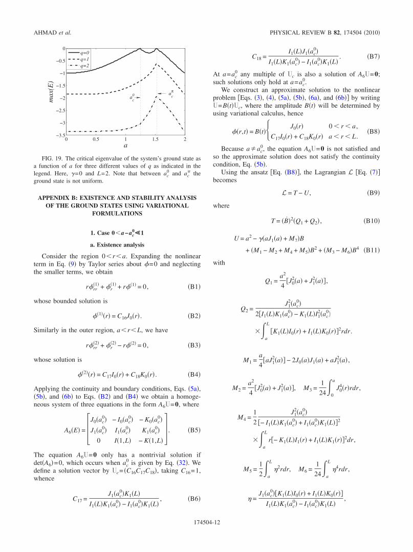
It is important to note that from the case of one-dimensional long 0-� Josephson junctions, the bifurcation ofthe nonuniform ground states from the uniform solutions issupercritical. One would therefore expect a similar situationin the present case. Hence, at the critical values ac the non-uniform ground states would satisfy the linearization of thegoverning Eq. �8� about the uniform solutions, which is thelinear eigenvalue problem �Eq. �12�� at E=0. On the otherhand, from the analysis of the uniform solutions, the criticaleigenvalue of the solutions corresponds to a independenteigenfunction �see also Fig. 19�. This then informs us that thenonuniform ground state should be independent �at leastnear ac�, i.e., Eq. �9�, which implies that �=0 in Eq. �7�.

Numerically we solve Eq. �9� using a finite differencemethod described in Appendix A. After obtaining the solu-tions, we calculate the critical eigenvalue, i.e., the smallesteigenfrequency, which defines the stability of the nonuniformground state. As in the analysis of uniform solutions, thecritical eigenvalue of our nonuniform ground state also cor-responds to the case of q=0 �see Appendix A�.

In addition to the numerical results, we also study theground states perturbatively using Euler-Lagrange approxi-mations when a is in the vicinity of the critical facet lengthac

0 or ac�. The method is as follows.

If ���r ;a� is an eigenfunction corresponding to the criticaleigenvalue � of a uniform solution � with the phase-discontinuity jump at r=a, then we construct an approximatesolution for 0�a−ac

0�1 and 0�ac�−a�1 to the nonlinear

problem �Eqs. �3�, �4�, �5a�, �5b�, �6a�, and �6b�� with0� ����1 by writing, respectively,

��r,t� = B�t��0�r;ac0�, B�t����r;ac

�� , �53�

where the amplitude B�t� will be determined by using varia-tional calculus. It is an approximate solution as for a�ac thefunction does not satisfy the continuity condition, Eq. �5b�.

Using the approximate solution and performing the inte-gration, the Lagrangian L �Eq. �7�� becomes a function ofB�t� and its first derivative. The Euler-Lagrange equation

�L�B

−d

dt �L

�B� = 0, �54�

then gives us

aπc

E

a

−1 −0.5 0 0.5 10

0.5

1

1.5

2

FIG. 6. �Color online� Plot of the discrete spectrum of the uni-form solution �0=� as a function of a for L=2.

AHMAD et al. PHYSICAL REVIEW B 82, 174504 �2010�

174504-6

B = F�B� . �55�

The time-independent value B=Bs that will make the ansatz�Eq. �53�� a good approximation is provided by a stationarypoint of the Lagrangian, i.e., it satisfies F�Bs�=0. Note that Fis also a function of a and �.

The variational formulation above can also provide solu-tions for small nonzero bias current. In general, the functionF will have three roots. When ��� increases, one will obtain avalue of � at which two solutions merge and disappear in asaddle-node bifurcation. This critical bias current can be cal-culated to satisfy

F�Bc� = 0,

where Bc is the root of �BF�B�=0.An approximation to the critical eigenvalue, i.e., the

smallest eigenfrequency, of the ground state can also be ob-tained using the result above. Linearizing Eq. �55� about the

fixed point Bs, i.e., substituting B=Bs+�B into Eq. �55�, oneobtains the equation

d2B

dt2 = �BF�Bs�B . �56�

The approximate critical eigenvalue is then given by

E = − �BF�Bs� ,

which is the square of the oscillation frequency of B�t�.

0 0.5 1 1.5 20.05

0.1

0.15

0.2

0.25

0.3

0.35

r

φ(r)

/π

−0.5 0 0.5−0.5

00.5

0.15

0.2

0.25

0.3

0.35

xy

φ/π

FIG. 7. �Color online� Top panel shows the numerically ob-tained ground state ��r� for L=2 and a=1.3 in the 1D representa-tion �solid� and its approximation �dashed�. Shown in the bottompanel is the corresponding profile in the original two-dimensionalproblem.

1.25 1.3 1.35 1.4 1.45 1.50

0.2

0.4

0.6

0.8

1

a

φ(0)

/π,φ

(a)/

π&

φ(L

)/π a

c0

acπ

1.25 1.3 1.35 1.4 1.45 1.5 1.550

0.1

0.2

0.3

0.4

0.5

0.6

0.7

0.8

a

∆φ

ac0

acπ

FIG. 8. �Color online� �Top panel� Comparisons of the numeri-cally obtained ground-state phases ��0�, ��L /2�, and ��L� �con-tinuous lines� and analytical approximations at a→ac

0 �see Eqs.�B8� and �B15�� �three lowest dotted lines� and approximations ata→ac

� �see Eqs. �B21� and �B24�� �three upper dotted lines� for�=0 and L=2. �Bottom panel� The difference of ��L�−��0� ob-tained numerically �solid� and analytically �dashed� in the vicinityof ac

0 and ac�.

2 3 4 50

0.2

0.4

0.6

0.8

1

a

φ(0)

/π

ac0

FIG. 9. �Color online� Similar to Fig. 8 but L→�.

−0.25 −0.2 −0.15 −0.1 −0.05 0 0.050

0.2

0.4

0.6

0.8

1

γ

φ(0)

/π

γc0

γcπ

FIG. 10. �Color online� Plot of ��0� as a function of �, calcu-lated numerically �solid� and approximated analytically �dashed� asgiven by Eqs. �B14� and �B23�. Here, a=1.3 and L=2.

EXISTENCE AND STABILITY ANALYSIS OF… PHYSICAL REVIEW B 82, 174504 �2010�

174504-7

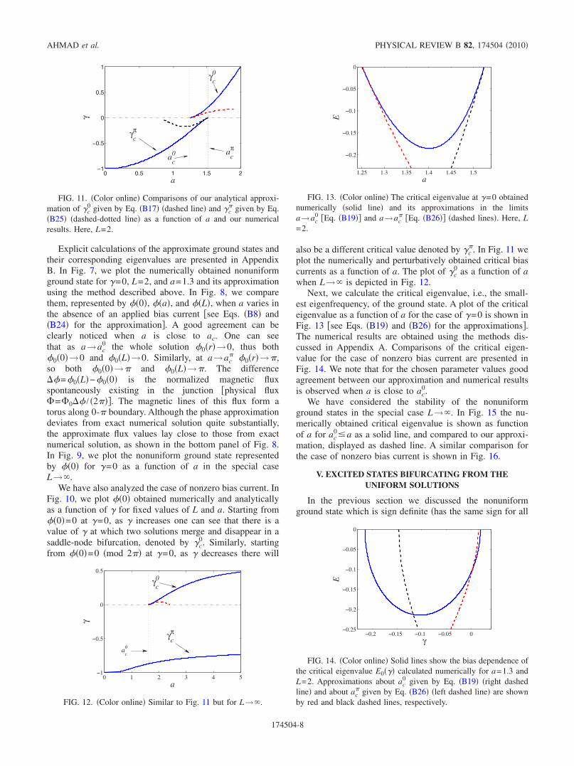
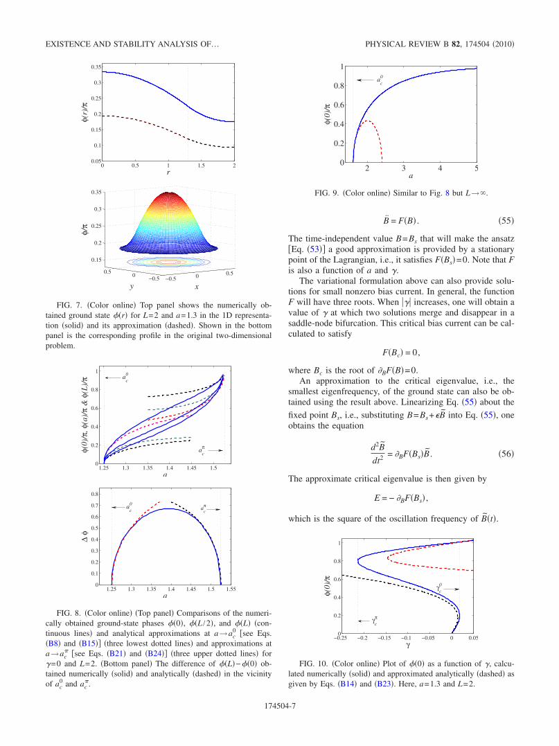
Explicit calculations of the approximate ground states andtheir corresponding eigenvalues are presented in AppendixB. In Fig. 7, we plot the numerically obtained nonuniformground state for �=0, L=2, and a=1.3 and its approximationusing the method described above. In Fig. 8, we comparethem, represented by ��0�, ��a�, and ��L�, when a varies inthe absence of an applied bias current �see Eqs. �B8� and�B24� for the approximation�. A good agreement can beclearly noticed when a is close to ac. One can seethat as a→ac

0 the whole solution �0�r�→0, thus both�0�0�→0 and �0�L�→0. Similarly, at a→ac

� �0�r�→�,so both �0�0�→� and �0�L�→�. The difference��=�0�L�−�0�0� is the normalized magnetic fluxspontaneously existing in the junction �physical flux�=�0�� / �2���. The magnetic lines of this flux form atorus along 0-� boundary. Although the phase approximationdeviates from exact numerical solution quite substantially,the approximate flux values lay close to those from exactnumerical solution, as shown in the bottom panel of Fig. 8.In Fig. 9, we plot the nonuniform ground state representedby ��0� for �=0 as a function of a in the special caseL→�.

We have also analyzed the case of nonzero bias current. InFig. 10, we plot ��0� obtained numerically and analyticallyas a function of � for fixed values of L and a. Starting from��0�=0 at �=0, as � increases one can see that there is avalue of � at which two solutions merge and disappear in asaddle-node bifurcation, denoted by �c

0. Similarly, startingfrom ��0�=0 �mod 2�� at �=0, as � decreases there will

also be a different critical value denoted by �c�. In Fig. 11 we

plot the numerically and perturbatively obtained critical biascurrents as a function of a. The plot of �c

0 as a function of awhen L→� is depicted in Fig. 12.

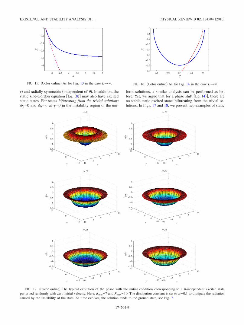
Next, we calculate the critical eigenvalue, i.e., the small-est eigenfrequency, of the ground state. A plot of the criticaleigenvalue as a function of a for the case of �=0 is shown inFig. 13 �see Eqs. �B19� and �B26� for the approximations�.The numerical results are obtained using the methods dis-cussed in Appendix A. Comparisons of the critical eigen-value for the case of nonzero bias current are presented inFig. 14. We note that for the chosen parameter values goodagreement between our approximation and numerical resultsis observed when a is close to ac

0.We have considered the stability of the nonuniform

ground states in the special case L→�. In Fig. 15 the nu-merically obtained critical eigenvalue is shown as functionof a for ac

0�a as a solid line, and compared to our approxi-mation, displayed as dashed line. A similar comparison forthe case of nonzero bias current is shown in Fig. 16.

V. EXCITED STATES BIFURCATING FROM THEUNIFORM SOLUTIONS

In the previous section we discussed the nonuniformground state which is sign definite �has the same sign for all

0 0.5 1 1.5 2−1

−0.5

0

0.5

1

a

γ

γcπ

acπ

γc0

ac0

FIG. 11. �Color online� Comparisons of our analytical approxi-mation of �c

0 given by Eq. �B17� �dashed line� and �c� given by Eq.

�B25� �dashed-dotted line� as a function of a and our numericalresults. Here, L=2.

0 1 2 3 4 5−1

−0.5

0

0.5

a

γ

ac0

γcπ

γc0

FIG. 12. �Color online� Similar to Fig. 11 but for L→�.

1.25 1.3 1.35 1.4 1.45 1.5

−0.2

−0.15

−0.1

−0.05

0

a

E

FIG. 13. �Color online� The critical eigenvalue at �=0 obtainednumerically �solid line� and its approximations in the limitsa→ac

0 �Eq. �B19�� and a→ac� �Eq. �B26�� �dashed lines�. Here, L

=2.

−0.2 −0.15 −0.1 −0.05 0−0.25

−0.2

−0.15

−0.1

−0.05

0

γ

E

FIG. 14. �Color online� Solid lines show the bias dependence ofthe critical eigenvalue E0��� calculated numerically for a=1.3 andL=2. Approximations about ac

0 given by Eq. �B19� �right dashedline� and about ac

� given by Eq. �B26� �left dashed line� are shownby red and black dashed lines, respectively.

AHMAD et al. PHYSICAL REVIEW B 82, 174504 �2010�

174504-8

r� and radially symmetric �independent of �. In addition, thestatic sine-Gordon equation �Eq. �8�� may also have excitedstatic states. For states bifurcating from the trivial solutions�0=0 and �0=� at �=0 in the instability region of the uni-

form solutions, a similar analysis can be performed as be-fore. Yet, we argue that for a phase shift �Eq. �4��, there areno stable static excited states bifurcating from the trivial so-lutions. In Figs. 17 and 18, we present two examples of static

2 2.5 3 3.5 4 4.5 5

−1

−0.8

−0.6

−0.4

−0.2

0

a

E

FIG. 15. �Color online� As for Fig. 13 in the case L→�.

−0.8 −0.6 −0.4 −0.2 0−0.8

−0.7

−0.6

−0.5

−0.4

−0.3

−0.2

−0.1

0

γ

E

FIG. 16. �Color online� As for Fig. 14 in the case L→�.

−10−5

05

10

−10

0

10−1.5

−1

−0.5

0

0.5

1

x

t=0

y

φ/π

−10−5

05

10

−10

0

10−1.5

−1

−0.5

0

0.5

1

x

t=13

y

φ/π

−10−5

05

10

−10

0

10−1.5

−1

−0.5

0

0.5

1

t=15

y

φ/π

−10−5

05

10

−10

−5

0

5

10−1.5

−1

−0.5

0

0.5

1

x

t=20

y

φ/π

−10−5

05

10

−10

0

10−1.5

−1

−0.5

0

0.5

1

t=25

y

φ/π

−10−5

05

10

−10

0

10−1.5

−1

−0.5

0

0.5

1

x

t=35

y

φ/π

FIG. 17. �Color online� The typical evolution of the phase with the initial condition corresponding to a -independent excited stateperturbed randomly with zero initial velocity. Here, Rmid=7 and Rmax=10. The dissipation constant is set to �=0.1 to dissipate the radiationcaused by the instability of the state. As time evolves, the solution tends to the ground state, see Fig. 7.

EXISTENCE AND STABILITY ANALYSIS OF… PHYSICAL REVIEW B 82, 174504 �2010�

174504-9

excited states bifurcating from the trivial solution �0�0 forRmid=7 and Rmax=10 and their typical instability dynamics,support our conjecture.

In Fig. 17, we present the dynamics of a -independentexcited state. This is an excited state in the sense that thesolution is not sign definite, i.e., it has one zero in the radialdirection. As for the excited state shown in Fig. 18, the stateis sign definite in the radial direction but not independent ofthe azimuthal direction ��. Defining the vorticity Q as thewave number of the oscillation or rotation in the azimuthaldirection, we note that the nonuniform ground state dis-cussed above and the excited state shown in Fig. 17 haveQ=0 while the excited state in Fig. 18 has vorticity Q=1. Wenote that both excited states will evolve into the ground stateshown in Fig. 7.

One may also obtain an excited state, which is a combi-nation of two types of states above. Yet, in this case, it willbe more unstable than those in Figs. 17 and 18.

VI. CONCLUSIONS

We have investigated a two-dimensional disk-shaped 0-�Josephson junction analytically and numerically both in thefinite and infinite domains. We have calculated the stabilityboundary of �0=0 and �0=� states. In the region of insta-bility of both �0=0 and �0=� states a semifluxon having ashape of a ring is generated spontaneously. Using an Euler-Lagrange formalism we have shown that the existence ofsemifluxons depends on the radius Rmax of the junction, theradius Rmid of 0-� boundary, and on the applied bias current.Critical eigenvalues that determine the stability of semi-fluxon solutions have been discussed as well. Analytical ex-pressions are compared with numerical simulations. We havebriefly discussed the existence of excited states bifurcatingfrom �0=0 and �0=� states, which are conjectured to beunstable for the particular phase-shift structure discussedhere.

−10−5

05

10

−10

0

10−1.5

−1

−0.5

0

0.5

1

t=0

y

φ/π

−10−5

05

10

−10

0

10−1.5

−1

−0.5

0

0.5

1

x

t=68

y

φ/π

−10−5

05

10

−10

−5

0

5

10−1.5

−1

−0.5

0

0.5

1

x

t=78

y

φ/π

−10−5

05

10

−10

0

10−1.5

−1

−0.5

0

0.5

1

x

t=85

y

φ/π

−10−5

05

10

−10

0

10−1.5

−1

−0.5

0

0.5

1

x

t=90

y

φ/π

−10−5

05

10

−10

0

10−1.5

−1

−0.5

0

0.5

1

x

t=105

y

φ/π

FIG. 18. �Color online� The same as Fig. 17 but for a static dependent excited state. As before, the solution also becomes the groundstate as t evolves.

AHMAD et al. PHYSICAL REVIEW B 82, 174504 �2010�

174504-10

Clearly, one is not limited by radially symmetric 0-�boundaries in 2D. One can easily fabricate and study 0-�boundaries having more arbitrary shapes in 2D includingself-crossing ones, e.g., checkerboardlike patterns. Such ge-ometries allow us to guide individual half-flux-quanta fieldlines in a predefined way and design devices that exploitthem. For example, one can use semifluxon strings as atransmission channel for transversal plasma waves, similar tothe situation discussed in Ref. 4.

ACKNOWLEDGMENTS

S.A. acknowledges support from the University of Mala-kand. E.G. thanks Deutsche Forschungsgemeinschaft�Project No. Go-1106/03� for financial support. H.S. thanksDarminto and the Department of Physics, Institut TeknologiSurabaya for their hospitality during the final stage of thepaper.

APPENDIX A: NUMERICAL SCHEMES AND THEANGULAR STABILITY

To solve numerically the independent Eq. �9�, whichcan be rewritten as

1

r�r�r�r = sin�� + � − � , �A1�

we use a finite difference method. We approximate the equa-tion by23

1

riri+1/2

�i+1 − �i

�r− ri−1/2

�i − �i−1

�r� 1

�r= sin��i + i� − � ,

�A2�

where �i and i, i=1, . . . , I, are the grid functions approxi-

mating ��i�r� and �i�r� and �r=L / �I+1�. The Dirichletboundary condition at r=L is approximated by

�I+1 = �I. �A3�

The most particular feature of polar coordinates is thecondition that must be imposed at r=0. To derive our condi-tion at the origin, we follow the method described in Ref. 23.Integrating Eq. �A1� over a small disk of radius � yields

0

�

�sin�� + � − ��rdr = 0

�

�r�r�rdr ,

where we have evaluated the integral over the angular vari-able as � is independent of . By assuming that in thesmall disk, � is independent of the radial variable r, theintegrals can be approximated by

sin��0 + 0��r

2�2

= �1 − �0, �A4�

where ���0 and = 0= 1. In the equation above, we havetaken �=�r /2 and approximated �r by a forward difference.Equations �A2�–�A4� form a complete set of algebraic equa-tions, which is solved using a Newton-Raphson method.

The eigenvalue problem �Eq. �14�� is also solved numeri-cally using a similar method. It is necessary to note that thesame calculation to obtain a condition at the origin as beforeshould not be applied directly to the equation. Instead, wefirst rewrite the equation as

r�rVr�r − q2V − r2 cos�� + �V = r2EV . �A5�

Integrating each term over a small disk yields

0

�

r�rVr�rrdr = �3Vr − 20

�

r2Vrdr

=�3Vr − 2�2V − 20

�

rVdr��

�r2

8�V1 − V0� ,

0

�

q2Vrdr ��r2

8q2V0,

0

�

�r2 cos�� + �V�rdr ��r4

64cos��0 + 0�V0,

0

�

�r2EV�rdr ��r4

64EV0.

The finite difference version of Eq. �A5� at the origin istherefore given by

V1 − �1 + q2 −�r2

8cos��0 + 0��V0 =

�r2

8EV0. �A6�

The boundary condition at r=L follows from Eq. �A3�,i.e.,

VI+1 = VI. �A7�

At the inner points, the eigenvalue problem �Eq. �A5�� isapproximated by

riri+1/2Vi+1 − Vi

�r− ri−1/2

Vi − Vi−1

�r� 1

�r− q2Vi

− ri2 cos��i + i�Vi = ri

2EVi. �A8�

Equations �A8� with boundary conditions �Eqs. �A6� and�A7�� form a generalized algebraic eigenvalue problem thathas to be solved simultaneously for �Vi i=0

I and E.We solve the two-dimensional time-independent equation

�Eq. �8�� using a Newton-Raphson method and numericallyintegrate the time-dependent one �Eq. �3�� using a Runge-Kutta method with a similar boundary condition at the sin-gularity r=0.23

We have used the method explained above to solve theeigenvalue problem �Eq. �14��. Shown in Fig. 19 is the criti-cal eigenvalue, i.e., the maximum E, of the system’s groundstate as a function of the radius a of the � region for threedifferent values of q, with L=2 and �=0. We note that thecase q=0 indeed gives the largest eigenvalue.

EXISTENCE AND STABILITY ANALYSIS OF… PHYSICAL REVIEW B 82, 174504 �2010�

174504-11

APPENDIX B: EXISTENCE AND STABILITY ANALYSISOF THE GROUND STATES USING VARIATIONAL

FORMULATIONS

1. Case 0�a−ac0™1

a. Existence analysis

Consider the region 0�r�a. Expanding the nonlinearterm in Eq. �9� by Taylor series about �=0 and neglectingthe smaller terms, we obtain

r�rr�1� + �r

�1� + r��1� = 0, �B1�

whose bounded solution is

��1��r� = C16J0�r� . �B2�

Similarly in the outer region, a�r�L, we have

r�rr�2� + �r

�2� − r��2� = 0, �B3�

whose solution is

��2��r� = C17I0�r� + C18K0�r� . �B4�

Applying the continuity and boundary conditions, Eqs. �5a�,�5b�, and �6b� to Eqs. �B2� and �B4� we obtain a homoge-neous system of three equations in the form A6U=0, where

A6�E� = �J0�ac0� − I0�ac

0� − K0�ac0�

J1�ac0� I1�ac

0� K1�ac0�

0 I�1,L� − K�1,L�� . �B5�

The equation A6U=0 only has a nontrivial solution ifdet�A6�=0, which occurs when ac

0 is given by Eq. �32�. Wedefine a solution vector by Uc= �C16C17C18�, taking C16=1,whence

C17 =J1�ac

0�K1�L�I1�L�K1�ac

0� − I1�ac0�K1�L�

, �B6�

C18 =I1�L�J1�ac

0�I1�L�K1�ac

0� − I1�ac0�K1�L�

. �B7�

At a=ac0 any multiple of Uc is also a solution of A6U=0;

such solutions only hold at a=ac0.

We construct an approximate solution to the nonlinearproblem �Eqs. �3�, �4�, �5a�, �5b�, �6a�, and �6b�� by writingU=B�t�Uc, where the amplitude B�t� will be determined byusing variational calculus, hence

��r,t� = B�t�� J0�r� 0 � r � a ,

C17I0�r� + C18K0�r� a � r � L .� �B8�

Because a�ac0, the equation A6U=0 is not satisfied and

so the approximate solution does not satisfy the continuitycondition, Eq. �5b�.

Using the ansatz �Eq. �B8��, the Lagrangian L �Eq. �7��becomes

L = T − U , �B9�

where

T = �B�2�Q1 + Q2� , �B10�

U = a2 − ��aJ1�a� + M7�B

+ �M1 − M2 + M4 + M5�B2 + �M3 − M6�B4 �B11�

with

Q1 =a2

4�J0

2�a� + J12�a�� ,

Q2 =J1

2�ac0�

2�I1�L�K1�ac0� − K1�L�I1

2�ac0��

�a

L

�K1�L�I0�r� + I1�L�K0�r��2rdr .

M1 =a

4�aJ1

2�a�� − 2J0�a�J1�a� + aJ12�a� ,

M2 =a2

4�J0

2�a� + J12�a��, M3 =

1

24

0

a

J04�r�rdr ,

M4 =1

2

J12�ac

0��− I1�L�K1�ac

0� + I1�ac0�K1�L��2

�a

L

r�− K1�L�I1�r� + I1�L�K1�r��2dr ,

M5 =1

2

a

L

�2rdr, M6 =1

24

a

L

�4rdr ,

� =J1�ac

0��K1�L�I0�r� + I1�L�K0�r��I1�L�K1�ac

0� − I1�ac0�K1�L�

,

0 0.5 1 1.5 2−3.5

−3

−2.5

−2

−1.5

−1

−0.5

0

a

max

(E)

q=0q=1q=2

ac0 a

cπ

FIG. 19. The critical eigenvalue of the system’s ground state asa function of a for three different values of q as indicated in thelegend. Here, �=0 and L=2. Note that between ac

0 and ac� the

ground state is not uniform.

AHMAD et al. PHYSICAL REVIEW B 82, 174504 �2010�

174504-12

M7 =J1�ac

0��2a�K1�L�I1�a� − I1�L�K�a�� + aI1�L��K0�a�I�a� + K1�a�I0�a�� − LI1�L��K1�L�I0�L� + I1�L�K0�L��

2�I1�ac0�K1�L� − I1�L�K1�ac

0��.

The Euler-Lagrange equation �Eq. �54�� gives us

B = f�B� , �B12�

where

f�B� =��aJ1�a� + M7� − 2�M1 − M2 + M4 + M5�B + 4�M6 − M3�B3

2�Q1 + Q2�. �B13�

The fixed points of this equation are given by f�B�=0, i.e.,UB=0.

The general solutions to the cubic equation, Eq. �B13�, for��0 can be found by using Nickall’s method,24 to yield

B�n� = 2� cos�� + �2n − 1��

3�, n = 1,2,3, �B14�

where

� =�M1 − M2 + M4 + M5

6�M6 − M3�,

h = − 2

3�3/2 �M1 − M2 + M4 + M5�3/2

�M6 − M3�1/2 ,

� =1

3arccos�− ��aJ1�a� + M7�

h� .

When �=0, the three roots above are simplified to

B�1,2� = ��M1 − M2 + M4 + M5

2�M6 − M3�, B�3� = 0. �B15�

It can be easily verified that the potential energy U islocally minimized by B�1� or B�2�. Hence, we obtain an ap-proximation to the nonuniform ground state in the instabilityregion of the constant solutions.

As the bias current � varies, there are two critical biascurrents at which two of the roots merge in a bifurcation,which can be calculated as follows.

Solving f��B�=0 for B, we obtain

Bc1,c2= ��M1 − M2 + M4 + M5

6�M6 − M3�. �B16�

These values of B locally minimize the potential energy U ofthe junction. The critical bias current �c

0 is then given by theinverse of f evaluated at Bc1,c2

above, i.e.,

�c0 = �

4�M6 − M3�Bc3 − 2�M1 − M2 + M4 + M5�Bc

aJ1�a� + M7.

�B17�

b. Stability analysis

To find the critical eigenvalue of the ground state analyti-

cally, we substitute B=B�n�+�B into Eq. �B12� and neglectthe higher order terms in � to obtain

d2B

dt2 = −6�M3 − M6��B�n��2 + �M1 − M2 + M4 + M5�

Q1 + Q2B .

�B18�

The critical eigenvalue of the ground state is therefore ap-proximately given by

E = −6�M3 − M6��B�n��2 + �M1 − M2 + M4 + M5�

Q1 + Q2,

�B19�

which is the square of the oscillation frequency of B�t�.

c. Infinite domain case

In the limit L→�, a similar calculation can be performedas before. Only in this case, for a close to ac

0, our approxi-mate ��r� �Eq. �B8�� becomes

��r� = B�t�� J0�r� 0 � r � a ,

J0�ac0����

K0�ac0����

K0�r� a � r � � ,� �B20�

i.e., C17→0 when L→� as limr→� I0�r�→�.

2. Case of 0�ac�−a™1

For a close to ac�, ��r� is approximated by

��r,t� = � − B�t�� C20I0�r� 0 � r � a ,

C21J0�r� + C22Y0�r� a � r � L .��B21�

Setting C20=1, the constants C21 and C22 are then given by

EXISTENCE AND STABILITY ANALYSIS OF… PHYSICAL REVIEW B 82, 174504 �2010�

174504-13

C21 =I1�ac

��Y1�L�J1�L�Y1�ac

�� − J1�ac��Y1�L�

,

C22 = −J1�L�I1�ac

��J1�L�Y1�ac

�� − J1�ac��Y1�L�

,

with ac� given by Eq. �46�.

The Lagrangian L=T−U is given by

T = �Q5 + Q6��B�2,

U = �M20 − M17�B4 + �M15 + M16 + M18 − M19�B2

− �a

2�a� + 2BI1�a�� +

��L2 − a2�2

B + M21B� + L2 − a2,

with

Q5 = −a2

4�− �I0�a��2 + �I1�a��2 ,

Q6 =I0�ac

��2

a

L

�rdr ,

� =Y1�L�J0�r� − J1�L�Y0�r�

J1�L�Y1�ac�� − J1�ac

��Y1�L�,

M15 =a2

4��I1�a��2 − I0�a�I2�a� ,

M16 =a2

4�I1�a�2 − I0�a�2�, M17 =

1

24

0

a

�I0�r��4rdr ,

M18 =1

2

a

L

R1rdr, M19 =1

2

a

L

R2rdr ,

M20 =1

24

a

L

R34rdr, M21 =

a

L

R3rdr ,

R1 = � I1�ac���J1�L�Y1�r� − Y1�L�J1�r��

J1�L�Y1�ac�� − Y1�L�J1�ac

�� �2

,

R2 = � I1�ac���J1�L�Y0�r� − Y1�L�J0�r��

Y1�L�J1�ac�� − J1�L�Y1�ac

�� �2

,

R3 =I1�ac

���J1�L�Y0�r� − Y1�L�J0�r��Y1�L�J1�ac

�� − J1�L�Y1�ac��

.

The Euler-Lagrange equation �Eq. �54�� becomes

d2B

dt2 = g�B� ,

where

g�B� = ��M20 − M17�B3 + 2�M15 + M16 + M18 − M19�B

− ��2I1�a� +�

2�L2 − a2� + M21��/2�Q3 + Q4�

�B22�

The fixed points of this equation are given by g�B�=0,which can be solved as before to yield

B�n� = 2� cos�� + �2n − 1��

3�, n = 1,2,3, �B23�

where

� =�M15 + M16 + M18 − M19

6�M20 − M17�,

h = − 2

3�3/2 �M15 + M16 + M18 − M19�3/2

�M20 − M17

,

� =1

3arccos�

h�2I1�a� +

�

2�L2 − a2� + M21�� .

For �=0, the roots are

B�1,2� = ��M15 + M16 + M18 − M19

2�M17 − M20�, B�3� = 0.

�B24�

Considering the nonzero roots B�1,2�, we find an approxima-tion to the ground state B as a function of a and � for 0�ac

�−a�1. We also note that there will again be a criticalbias current �c

� at which a saddle-node bifurcation occurs. Ina similar manner to above, it can be easily calculated that thecritical bias current is approximately given by

�c� =

4�M20 − M17�Bc3 + 2�M15 + M16 + M18 − M19�Bc

2I1�a� +�

2�L2 − a2� + M21

.

�B25�

The critical eigenvalue of the nonuniform ground states inthis case can be readily calculated as

E = −6�M17 − M20��B�n��2 − �M15 + M16 + M18 − M19�

Q5 + Q6.

�B26�

AHMAD et al. PHYSICAL REVIEW B 82, 174504 �2010�

174504-14

*On leave from Department of Mathematics, Universityof Malakand, Chakdara, K. Pakhtunkhwa, Pakistan;[email protected]

†[email protected] A. V. Ustinov, Physica D 123, 315 �1998�.2 J. Zagrodzinski, Phys. Lett. A 57, 213 �1976�.3 P. L. Christiansen and P. S. Lomdahl, Physica D 2, 482 �1981�.4 D. R. Gulevich, F. V. Kusmartsev, S. Savel’ev, V. A.

Yampol’skii, and F. Nori, Phys. Rev. B 80, 094509 �2009�.5 It is believed that the spatially uniform sine-Gordon equation has

no radially symmetric �angle independent� static solitonic solu-tions in two or more spatial dimensions �Ref. 25�. In fact, theargument given in Ref. 25 applies only to three or more spatialdimensions and fails in 2D. Still, in 2D the static ring soliton isunstable and collapses to the center as it has infinite criticalradius at zero bias �Ref. 26�.

6 In fact, any radially symmetric solution ��r� of anN-dimensional sine-Gordon equation �Ref. 25� is equivalent to asolution ��x� of a one-dimensional sine-Gordon equation withvariable �Josephson junction� width �Ref. 27� w�x�= �N−1�x.

7 P. L. Christiansen and O. H. Olsen, Phys. Lett. A 68, 185 �1978�.8 J. Geicke, Phys. Scr. 29, 431 �1984�.9 B. A. Malomed, Physica D 24, 155 �1987�.

10 L. N. Bulaevski�, V. V. Kuzi�, and A. A. Sobyanin, JETP Lett.25, 290 �1977�.

11 A. I. Buzdin, L. N. Bulaevskii, and S. V. Panyukov, JETP Lett.35, 178 �1982�.

12 V. A. Oboznov, V. V. Bol’ginov, A. K. Feofanov, V. V. Ryaza-nov, and A. I. Buzdin, Phys. Rev. Lett. 96, 197003 �2006�.

13 T. Kontos, M. Aprili, J. Lesueur, F. Genêt, B. Stephanidis, and R.

Boursier, Phys. Rev. Lett. 89, 137007 �2002�.14 M. Weides, M. Kemmler, E. Goldobin, D. Koelle, R. Kleiner, H.

Kohlstedt, and A. Buzdin, Appl. Phys. Lett. 89, 122511 �2006�.15 O. Vavra, S. Gazi, D. S. Golubovic, I. Vavra, J. Derer, J. Ver-

beeck, G. Van Tendeloo, and V. V. Moshchalkov, Phys. Rev. B74, 020502 �2006�.

16 H. Hilgenkamp, Ariando, H.-J. H. Smilde, D. H. A. Blank, G.Rijnders, H. Rogalla, J. R. Kirtley, and C. C. Tsuei, Nature�London� 422, 50 �2003�.

17 M. Weides, M. Kemmler, H. Kohlstedt, R. Waser, D. Koelle, R.Kleiner, and E. Goldobin, Phys. Rev. Lett. 97, 247001 �2006�.

18 E. Goldobin, A. Sterck, T. Gaber, D. Koelle, and R. Kleiner,Phys. Rev. Lett. 92, 057005 �2004�.

19 L. N. Bulaevskii, V. V. Kuzii, and A. A. Sobyanin, Solid StateCommun. 25, 1053 �1978�.

20 C. Gürlich, S. Scharinger, M. Weides, H. Kohlstedt, R. G. Mints,E. Goldobin, D. Koelle, and R. Kleiner, Phys. Rev. B 81,094502 �2010�.

21 Handbook of Mathematical Functions with Formulas, Graphs,and Mathematical Tables, edited by M. Abramowitz and I. A.Stegun �Dover, New York, 1974�.

22 E. Goldobin, D. Koelle, and R. Kleiner, Phys. Rev. B 67,224515 �2003�.

23 Finite Difference Schemes and Partial Differential Equations, J.Strikwerda �SIAM, Philadelphia, 2004�.

24 R. Nickalls, Math. Gaz. 77, 354 �1993�.25 G. H. Derrick, J. Math. Phys. 5, 1252 �1964�.26 O. H. Olsen and M. R. Samuelsen, Phys. Scr. 23, 1033 �1981�.27 E. Goldobin, A. Sterck, and D. Koelle, Phys. Rev. E 63, 031111

�2001�.

EXISTENCE AND STABILITY ANALYSIS OF… PHYSICAL REVIEW B 82, 174504 �2010�

174504-15