24 May 2021 EXERCISE SOLUTIONS for COMPUTATION AND PROBLEM SOLVING IN UNDERGRADUATE PHYSICS • IDL MATLAB OCTAVE PYTHON MAXIMA MAPLE • MATHEMATICA • PROGRAM • FORTRAN • C LSODE PDEs MUDPACK • L A T E X TGIF DAVID M. COOK with assistance from DANICA DRALUS, LU ’02 RYAN PETERSON, LU ’03 SCOTT KAMINSKI, LU ’04 MICHELLE MILNE, LU ’04 LAUREN KOST, LU ’05 CLAIRE WEISS, LU ’07 ERIK GARBACIK, LU ’08 Department of Physics Lawrence University 711 E Boldt Way SPC 24 Appleton, Wisconsin 54911 Copyright c 2000–21 by David M. Cook This work is licensed under a Creative Commons Attribution-NonCommercial- ShareAlike 4.0 International License (creativecommons.org/licenses/by-nc-sa/4.0/). Any use not permitted by this license requires authorization in writing from David M. Cook.

Welcome message from author
This document is posted to help you gain knowledge. Please leave a comment to let me know what you think about it! Share it to your friends and learn new things together.
Transcript
24 May 2021
EXERCISE SOLUTIONSfor
COMPUTATION AND PROBLEM SOLVING
IN UNDERGRADUATE PHYSICS
• IDL MATLAB OCTAVE
PYTHON MAXIMA MAPLE
• MATHEMATICA • PROGRAM • FORTRAN
• C LSODE PDEs
MUDPACK • LATEX TGIF
DAVID M. COOKwith assistance from
DANICA DRALUS, LU ’02 RYAN PETERSON, LU ’03
SCOTT KAMINSKI, LU ’04 MICHELLE MILNE, LU ’04
LAUREN KOST, LU ’05 CLAIRE WEISS, LU ’07
ERIK GARBACIK, LU ’08
Department of PhysicsLawrence University
711 E Boldt Way SPC 24Appleton, Wisconsin 54911
Copyright c© 2000–21 by David M. Cook
This work is licensed under a Creative Commons Attribution-NonCommercial-ShareAlike 4.0 International License (creativecommons.org/licenses/by-nc-sa/4.0/).Any use not permitted by this license requires authorization in writing from DavidM. Cook.

ii
Preface
This document contains solutions to selected exercises from Computation and Problem Solving inUndergraduate Physics (CPSUP), a book that has grown from small beginnings in the 1990s to aflexible volume that provides an orientation to a subset of tools chosen from
• the general purpose programs IDL, MATLAB, OCTAVE, PYTHON, MAXIMA, MAPLE, andMATHEMATICA,
• the programming languages FORTRAN and C,
• FORTRAN NUMERICAL RECIPES,
• C NUMERICAL RECIPES,
• the FORTRAN procedure library LSODE,
• the UNIX drawing program TGIF, and
• the tool LATEX for preparation of technical documents.
In addition, chapters on ordinary differential equations, integration, and root finding provide ex-amples of the use of the selected subset of tools for solving a wide variety of problems in physics.Problems from mechanics, electromagnetic theory, quantum mechanics, thermodynamics, statisticalmechanics, relativity, and other subarea of physics are included.
This document admits the same flexibility in composition that characterizes CPSUP. Both CP-SUP and this document can be configured to include all of the possibilities or only a selected subsetof the options. Because there are 13 different components, each of which can be included or not,there are technically 213 = 8012 versions of these items. To be sure, the vast majority of thesepossibilities makes no sense. Still, the number of versions is staggering. Creating documents withthis degree of flexibility would be impossible without exploiting the elegant features of the ifthen
package in LATEX, and I owe an immense debt to Donald Knuth, Leslie Lamport, and numerousothers who have contributed to the development of that publishing system.
iii

iv PREFACE
Table of Contents
Preface iii
Table of Contents v
2 Introduction to IDL 1
2.1 Creating Vectors and Matrices . . . . . . . . . . . . . . . . . . . . . . . . . . . . . . . . . 12.2 Properties of sort . . . . . . . . . . . . . . . . . . . . . . . . . . . . . . . . . . . . . . . . 32.5 Summing Elements in a Vector . . . . . . . . . . . . . . . . . . . . . . . . . . . . . . . . . 52.6 Evaluating a Cross Product . . . . . . . . . . . . . . . . . . . . . . . . . . . . . . . . . . . 62.8 Eigenvectors/Values in a Single Matrix . . . . . . . . . . . . . . . . . . . . . . . . . . . . 7
2.9 Finding/Plotting Eigenvalues/Vectors . . . . . . . . . . . . . . . . . . . . . . . . . . . . . 82.10 Stark Effect for n = 2 and n = 3 . . . . . . . . . . . . . . . . . . . . . . . . . . . . . . . . 152.11 Damped and Undamped Sine Waves . . . . . . . . . . . . . . . . . . . . . . . . . . . . . . 182.13 Plotting the Potential of a Charged Disk . . . . . . . . . . . . . . . . . . . . . . . . . . . 192.14 A Charging Capacitor . . . . . . . . . . . . . . . . . . . . . . . . . . . . . . . . . . . . . . 202.15 Plotting the Output of a Fabry-Perot Interferometer . . . . . . . . . . . . . . . . . . . . . 212.17 Plotting Common Relativistic Functions . . . . . . . . . . . . . . . . . . . . . . . . . . . . 232.18 Plotting Transmission/Reflection of Thin Film . . . . . . . . . . . . . . . . . . . . . . . . 252.19 Plotting the Potential of Two Charged Disks . . . . . . . . . . . . . . . . . . . . . . . . . 272.22 Plotting Relativistic Functions: Compton Effect . . . . . . . . . . . . . . . . . . . . . . . 292.23 Field of a Moving Charge . . . . . . . . . . . . . . . . . . . . . . . . . . . . . . . . . . . . 322.24 Plotting the Four-Slit Interference Pattern . . . . . . . . . . . . . . . . . . . . . . . . . . 352.25 Plotting the Planck Blackbody Radiation Curve . . . . . . . . . . . . . . . . . . . . . . . 382.26 Plotting the On-Axis Field of a Solenoid . . . . . . . . . . . . . . . . . . . . . . . . . . . 422.27 Plotting the On-Axis Field of a Pair of Current Loops . . . . . . . . . . . . . . . . . . . . 482.28 Current in an LRC Circuit . . . . . . . . . . . . . . . . . . . . . . . . . . . . . . . . . . . 512.30 Cooking a Spherical Potato . . . . . . . . . . . . . . . . . . . . . . . . . . . . . . . . . . . 532.31 Gravitational Potential Energy in a Plane . . . . . . . . . . . . . . . . . . . . . . . . . . . 582.32 Plotting Probability Densities in Hydrogen . . . . . . . . . . . . . . . . . . . . . . . . . . 632.33 Standing Waves in a Cube . . . . . . . . . . . . . . . . . . . . . . . . . . . . . . . . . . . 692.38 Animation of a Vibrating String . . . . . . . . . . . . . . . . . . . . . . . . . . . . . . . . 762.39 Animation of a User Function . . . . . . . . . . . . . . . . . . . . . . . . . . . . . . . . . 802.40 Animation of a Square Membrane . . . . . . . . . . . . . . . . . . . . . . . . . . . . . . . 84
8 Introduction to Mathematica 87
8.2 A Few MATHEMATICA Manipulations . . . . . . . . . . . . . . . . . . . . . . . . . . . . 878.3 More MATHEMATICA Manipulations . . . . . . . . . . . . . . . . . . . . . . . . . . . . 898.5 Legendre Polynomials . . . . . . . . . . . . . . . . . . . . . . . . . . . . . . . . . . . . . . 928.6 Wheatstone Bridge . . . . . . . . . . . . . . . . . . . . . . . . . . . . . . . . . . . . . . . . 1008.7 Quantum Wave Scattering . . . . . . . . . . . . . . . . . . . . . . . . . . . . . . . . . . . 1038.8 Black Body Spectrum . . . . . . . . . . . . . . . . . . . . . . . . . . . . . . . . . . . . . . 1068.10 Laguerre Polynomials . . . . . . . . . . . . . . . . . . . . . . . . . . . . . . . . . . . . . . 1108.12 Finding Eigenvectors/Values . . . . . . . . . . . . . . . . . . . . . . . . . . . . . . . . . . 1158.13 Stark Effect for n = 2 and n = 3 . . . . . . . . . . . . . . . . . . . . . . . . . . . . . . . . 1188.14 Lagrangian Approach to Equations of Motion . . . . . . . . . . . . . . . . . . . . . . . . . 1228.16 Elliptic Integrals . . . . . . . . . . . . . . . . . . . . . . . . . . . . . . . . . . . . . . . . . 128
v
vi PREFACE
8.17 Laplace transforms . . . . . . . . . . . . . . . . . . . . . . . . . . . . . . . . . . . . . . . . 1308.18 Fitting Parabola Through Three Points . . . . . . . . . . . . . . . . . . . . . . . . . . . . 1328.19 Deducing Simpson’s Rule . . . . . . . . . . . . . . . . . . . . . . . . . . . . . . . . . . . . 1338.20 Accuracy of Simpson’s Rule . . . . . . . . . . . . . . . . . . . . . . . . . . . . . . . . . . . 1348.24 Vector Derivatives in Cylindrical Coordinates . . . . . . . . . . . . . . . . . . . . . . . . . 1368.26 Vector Product Identities . . . . . . . . . . . . . . . . . . . . . . . . . . . . . . . . . . . . 139
9 Introduction to Programming 141
in Psuedocode
9.2 Relationship between IF-THEN-ELSE and CASE . . . . . . . . . . . . . . . . . . . . . . 1419.7 Tracking Both Extremes and their Positions . . . . . . . . . . . . . . . . . . . . . . . . . 1449.9 Mystery Procedure 1 . . . . . . . . . . . . . . . . . . . . . . . . . . . . . . . . . . . . . . . 146
in FORTRAN
9.12 Conversion from Celsius to Fahrenheit (FORTRAN) . . . . . . . . . . . . . . . . . . . . . 148
9.13 Laplace’s Equation with Different Grids (FORTRAN) . . . . . . . . . . . . . . . . . . . . 150
9.16 Exploring Trajectories in 3D (FORTRAN) . . . . . . . . . . . . . . . . . . . . . . . . . . 160
9.22 Great Circle Distances (FORTRAN) . . . . . . . . . . . . . . . . . . . . . . . . . . . . . . 166
in C
9.12 Conversion from Celsius to Fahrenheit (C) . . . . . . . . . . . . . . . . . . . . . . . . . . 171
9.14 Laplace’s Equation with Different Grids (C) . . . . . . . . . . . . . . . . . . . . . . . . . 173
9.16 Exploring Trajectories in 3D (C) . . . . . . . . . . . . . . . . . . . . . . . . . . . . . . . . 183
9.22 Great Circle Distances (C) . . . . . . . . . . . . . . . . . . . . . . . . . . . . . . . . . . . 189
11 Solving ODEs 195
symbolically with Mathematica
11.1 Driven oscillator (Mathematica) . . . . . . . . . . . . . . . . . . . . . . . . . . . . . . . . 195
11.2 Two Masses, One Spring (Mathematica) . . . . . . . . . . . . . . . . . . . . . . . . . . . . 199
11.4 Compound Pendulum (Mathematica) . . . . . . . . . . . . . . . . . . . . . . . . . . . . . 204
11.6 Series Solution (Mathematica) . . . . . . . . . . . . . . . . . . . . . . . . . . . . . . . . . 208
11.7 Projectile in Linear Air Resistance (Mathematica) . . . . . . . . . . . . . . . . . . . . . . 212
11.12 Vibrating String Fixed at Both Ends (MATHEMATICA) . . . . . . . . . . . . . . . . . . 214
numerically with IDL
11.17 Van der Pol Oscillator (IDL) . . . . . . . . . . . . . . . . . . . . . . . . . . . . . . . . . . 216
11.18 Large Amplitude Pendulum (IDL) . . . . . . . . . . . . . . . . . . . . . . . . . . . . . . . 220
11.19 Planet in Non-Inverse Square Gravity (IDL) . . . . . . . . . . . . . . . . . . . . . . . . . 225
11.21 Satellite with Two Suns (IDL) . . . . . . . . . . . . . . . . . . . . . . . . . . . . . . . . . 228
11.22 Charge in Crossed Fields (IDL) . . . . . . . . . . . . . . . . . . . . . . . . . . . . . . . . . 232
11.24 The Lorenz Attractor (IDL) . . . . . . . . . . . . . . . . . . . . . . . . . . . . . . . . . . 237
11.27 Dynamics of a Chemical Reaction (IDL) . . . . . . . . . . . . . . . . . . . . . . . . . . . . 240
11.28 The Predator-Prey Problem (IDL) . . . . . . . . . . . . . . . . . . . . . . . . . . . . . . . 244
numerically with FORTRAN
11.25 Radioactive Decay (FORTRAN) . . . . . . . . . . . . . . . . . . . . . . . . . . . . . . . . 247
numerically with C
11.26 Radioactive Decay (C) . . . . . . . . . . . . . . . . . . . . . . . . . . . . . . . . . . . . . . 252
numerically with Numerical Recipes in FORTRAN
11.33 Logistic Growth (Numerical Recipes-FORTRAN) . . . . . . . . . . . . . . . . . . . . . . 257
11.36 Lorenz System (Numerical Recipes-FORTRAN) . . . . . . . . . . . . . . . . . . . . . . . 263
numerically with Numerical Recipes in C
PREFACE vii
11.33 Logistic Growth (Numerical Recipes-C) . . . . . . . . . . . . . . . . . . . . . . . . . . . . 269
11.36 Lorenz system (Numerical Recipes-C) . . . . . . . . . . . . . . . . . . . . . . . . . . . . . 275
13 Evaluating Integrals 281
symbolically with Mathematica
13.1 Non-relativistic Motion under Constant Force (MATHEMATICA) . . . . . . . . . . . . . 281
13.2 Non-relativistic Motion under Constant Force (MATHEMATICA) . . . . . . . . . . . . . 282
13.3 Non-relativistic Motion under Spring Force (MATHEMATICA) . . . . . . . . . . . . . . 284
13.4 Non-Relativistic Motion with Decaying Force (Mathematica) . . . . . . . . . . . . . . . . 287
13.5 Properties of Lorentz Distribution (Mathematica) . . . . . . . . . . . . . . . . . . . . . . 289
13.6 Earth Falling into Sun (Mathematica) . . . . . . . . . . . . . . . . . . . . . . . . . . . . . 291
13.7 Electron inside Bohr Radius (Mathematica) . . . . . . . . . . . . . . . . . . . . . . . . . 294
13.8 On-Axis Potential of a Pair of Disks (Mathematica) . . . . . . . . . . . . . . . . . . . . . 296
13.10 Properties of Cardioid (Mathematica) . . . . . . . . . . . . . . . . . . . . . . . . . . . . . 299
13.11 Oscillator Matrix Elements (Mathematica) . . . . . . . . . . . . . . . . . . . . . . . . . . 302
13.12 Fourier Coefficients for Sawtooth (Mathematica) . . . . . . . . . . . . . . . . . . . . . . . 308
13.13 Expansion in Legendre Polynomials (MATHEMATICA) . . . . . . . . . . . . . . . . . . . 310
13.14 Deduction of Simpson’s Rule (Mathematica) . . . . . . . . . . . . . . . . . . . . . . . . . 313
numerically with IDL
13.18 Quantum Harmonic Oscillator Turning Points (IDL) . . . . . . . . . . . . . . . . . . . . . 315
13.19 Maxwell-Boltzmann Distribution (IDL) . . . . . . . . . . . . . . . . . . . . . . . . . . . . 317
13.20 Black Body Radiation (IDL) . . . . . . . . . . . . . . . . . . . . . . . . . . . . . . . . . . 319
13.21 Confidence Intervals for Gaussian (IDL) . . . . . . . . . . . . . . . . . . . . . . . . . . . . 322
13.22 Earth Falling into Sun (IDL) . . . . . . . . . . . . . . . . . . . . . . . . . . . . . . . . . . 324
13.23 Properties of Lorentz Distribution (IDL) . . . . . . . . . . . . . . . . . . . . . . . . . . . 326
13.24 Electron inside Bohr Radius (IDL) . . . . . . . . . . . . . . . . . . . . . . . . . . . . . . . 327
13.25 Elliptic Integrals (IDL) . . . . . . . . . . . . . . . . . . . . . . . . . . . . . . . . . . . . . 329
13.26 Large Amplitude Simple Pendulum (IDL) . . . . . . . . . . . . . . . . . . . . . . . . . . . 333
13.27 N-th Order Bessel Functions (IDL) . . . . . . . . . . . . . . . . . . . . . . . . . . . . . . . 336
13.28 The Bessel Function J1(x) (IDL) . . . . . . . . . . . . . . . . . . . . . . . . . . . . . . . . 338
13.29 Off-axis Potential of Circular Ring (IDL) . . . . . . . . . . . . . . . . . . . . . . . . . . . 340
13.30 Off-axis Field of Current Loop (IDL) . . . . . . . . . . . . . . . . . . . . . . . . . . . . . 343
numerically with Mathematica
13.20 Black Body Radiation (Mathematica) . . . . . . . . . . . . . . . . . . . . . . . . . . . . . 347
13.21 Confidence Intervals for Gaussian (Mathematica) . . . . . . . . . . . . . . . . . . . . . . . 349
13.23 Properties of Lorentz Distribution (Mathematica) . . . . . . . . . . . . . . . . . . . . . . 351
numerically with FORTRAN
13.32 Simpson’s Rule (FORTRAN) . . . . . . . . . . . . . . . . . . . . . . . . . . . . . . . . . 352
13.33 Gaussian Integration (FORTRAN) . . . . . . . . . . . . . . . . . . . . . . . . . . . . . . . 356
numerically with C
13.34 Simpson’s Rule (C) . . . . . . . . . . . . . . . . . . . . . . . . . . . . . . . . . . . . . . . 360
13.35 Gaussian Integration (C) . . . . . . . . . . . . . . . . . . . . . . . . . . . . . . . . . . . . 363
numerically with Numerical Recipes in FORTRAN
13.37 Numerical Integration (Numerical Recipes–FORTRAN) . . . . . . . . . . . . . . . . . . . 367
13.40 Maxwell-Boltzmann Distribution (Numerical Recipes–FORTRAN) . . . . . . . . . . . . . 369
numerically with Numerical Recipes in C
13.44 Numerical Integration (Numerical Recipes–C) . . . . . . . . . . . . . . . . . . . . . . . . 373
13.47 Maxwell-Boltzmann Distribution (Numerical Recipes–C) . . . . . . . . . . . . . . . . . . 375
viii PREFACE
14 Finding Roots 379
symbolically with Mathematica
14.3 Finding Extrema a Cubic Polynomial (Mathematica) . . . . . . . . . . . . . . . . . . . . . 379
14.4 Roots of Quadratic Equation (Mathematica) . . . . . . . . . . . . . . . . . . . . . . . . . 381
14.5 Lawnmower Blade Overlap (Mathematica) . . . . . . . . . . . . . . . . . . . . . . . . . . . 382
14.8 Three Coupled Oscillators (Mathematica) . . . . . . . . . . . . . . . . . . . . . . . . . . . 384
numerically with IDL
14.12 Square Root by Newton’s Method (IDL) . . . . . . . . . . . . . . . . . . . . . . . . . . . 388
14.14 Natural Frequencies of Bar (IDL) . . . . . . . . . . . . . . . . . . . . . . . . . . . . . . . 391
14.17 Finite Depth Square Well (IDL) . . . . . . . . . . . . . . . . . . . . . . . . . . . . . . . . 397
14.18 Single-Slit Diffraction (IDL) . . . . . . . . . . . . . . . . . . . . . . . . . . . . . . . . . . 403
14.19 Roots of J0(x) (IDL) . . . . . . . . . . . . . . . . . . . . . . . . . . . . . . . . . . . . . . 406
14.20 Double-Welled Potential (IDL) . . . . . . . . . . . . . . . . . . . . . . . . . . . . . . . . . 408
14.24 A Fluid Mechanics Problem (IDL) . . . . . . . . . . . . . . . . . . . . . . . . . . . . . . 411
numerically with Mathematica
14.18 Single-Slit Diffraction (Mathematica) . . . . . . . . . . . . . . . . . . . . . . . . . . . . . . 413
14.19 Roots of J0(x) (Mathematica) . . . . . . . . . . . . . . . . . . . . . . . . . . . . . . . . . . 417
14.20 Double-Welled Potential (Mathematica) . . . . . . . . . . . . . . . . . . . . . . . . . . . . 419
numerically with FORTRAN
14.12 Square Root by Newton’s Method (FORTRAN) . . . . . . . . . . . . . . . . . . . . . . . 421
14.25 Rootfinding with Newton’s Method (FORTRAN) . . . . . . . . . . . . . . . . . . . . . . . 424
numerically with C
14.12 Square Root by Newton’s Method (C) . . . . . . . . . . . . . . . . . . . . . . . . . . . . . 429
14.26 Rootfinding with Newton’s Method (C) . . . . . . . . . . . . . . . . . . . . . . . . . . . . 432
numerically with Numerical Recipes in FORTRAN
14.14 Natural Frequencies of Bar (NUMERICAL RECIPES-FORTRAN) . . . . . . . . . . . . 437
14.18 Single-Slit Diffraction (NUMERICAL RECIPES-FORTRAN) . . . . . . . . . . . . . . . . 443
14.19 Roots of J0(x) (NUMERICAL RECIPES-FORTRAN) . . . . . . . . . . . . . . . . . . . . 447
14.20 Double-Welled Potential (NUMERICAL RECIPES-FORTRAN) . . . . . . . . . . . . . . 449
14.24 A Fluid Mechanics Problem (NUMERICAL RECIPES-FORTRAN) . . . . . . . . . . . . 452
14.29 Finite Depth Square Well (NUMERICAL RECIPES-FORTRAN) . . . . . . . . . . . . . 455
numerically with Numerical Recipes in C
14.14 Natural Frequencies of Bar (NUMERICAL RECIPES-C) . . . . . . . . . . . . . . . . . . 463
14.18 Single-Slit Diffraction (NUMERICAL RECIPES-C) . . . . . . . . . . . . . . . . . . . . . 470
14.19 Roots of J0(x) (NUMERICAL RECIPES-C) . . . . . . . . . . . . . . . . . . . . . . . . . 474
14.20 Double-Welled Potential (NUMERICAL RECIPES-C) . . . . . . . . . . . . . . . . . . . . 476
14.24 A Fluid Mechanics Problem (NUMERICAL RECIPES-C) . . . . . . . . . . . . . . . . . 480
14.30 Finite Depth Square Well (NUMERICAL RECIPES-C) . . . . . . . . . . . . . . . . . . 483
A Introduction to LATEX 493
A.2 A Letter to a Friend . . . . . . . . . . . . . . . . . . . . . . . . . . . . . . . . . . . . . . . 493A.4 Chain Radioactive Decay . . . . . . . . . . . . . . . . . . . . . . . . . . . . . . . . . . . . 498
Chapter 2
Introduction to IDL
2.1 Creating Vectors and Matrices
Exercise: Write and test IDL statements to create (a) a five-element column vector, (b) an8× 8 unit matrix, and (c) a 10× 10 matrix all of whose elements are zero except those on the maindiagonal (which are all 2) and those on the diagonals just above and just below the main diagonal(which are all −1). Search for a route more efficient than laboriously setting each of the 100 elementsin the 10× 10 matrix individually.
Solution: (a) One way to create a column vector in IDL is to enclose each element in its ownpair of (square) brackets and then enclose the five elements themselves in a pair of brackets. Thestatements
IDL> colvec = [ [10], [8], [-5], [3], [12] ]
IDL> print,colvec
10
8
-5
3
12
achieve this objective. Alternatively, we could create a row vector and transpose it with the state-ments
IDL> rowvec = [ 10, 8, -5, 3, 12 ]
IDL> print, rowvec
10 8 -5 3 12
IDL> colvec = transpose( rowvec )
IDL> print, colvec
10
8
-5
3
12
1
2 Exercise 2.1
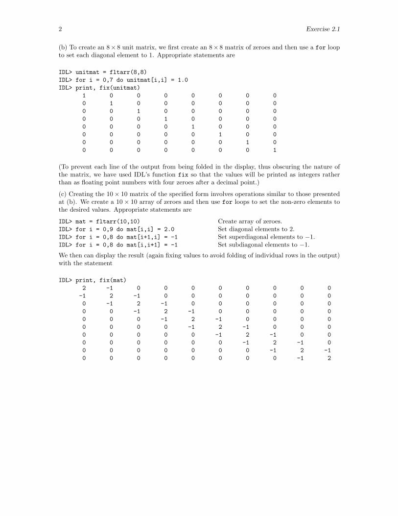
(b) To create an 8× 8 unit matrix, we first create an 8× 8 matrix of zeroes and then use a for loopto set each diagonal element to 1. Appropriate statements are
IDL> unitmat = fltarr(8,8)
IDL> for i = 0,7 do unitmat[i,i] = 1.0
IDL> print, fix(unitmat)
1 0 0 0 0 0 0 0
0 1 0 0 0 0 0 0
0 0 1 0 0 0 0 0
0 0 0 1 0 0 0 0
0 0 0 0 1 0 0 0
0 0 0 0 0 1 0 0
0 0 0 0 0 0 1 0
0 0 0 0 0 0 0 1
(To prevent each line of the output from being folded in the display, thus obscuring the nature ofthe matrix, we have used IDL’s function fix so that the values will be printed as integers ratherthan as floating point numbers with four zeroes after a decimal point.)
(c) Creating the 10× 10 matrix of the specified form involves operations similar to those presentedat (b). We create a 10× 10 array of zeroes and then use for loops to set the non-zero elements tothe desired values. Appropriate statements are
IDL> mat = fltarr(10,10)
IDL> for i = 0,9 do mat[i,i] = 2.0
IDL> for i = 0,8 do mat[i+1,i] = -1
IDL> for i = 0,8 do mat[i,i+1] = -1
Create array of zeroes.Set diagonal elements to 2.Set superdiagonal elements to −1.Set subdiagonal elements to −1.
We then can display the result (again fixing values to avoid folding of individual rows in the output)with the statement
IDL> print, fix(mat)
2 -1 0 0 0 0 0 0 0 0
-1 2 -1 0 0 0 0 0 0 0
0 -1 2 -1 0 0 0 0 0 0
0 0 -1 2 -1 0 0 0 0 0
0 0 0 -1 2 -1 0 0 0 0
0 0 0 0 -1 2 -1 0 0 0
0 0 0 0 0 -1 2 -1 0 0
0 0 0 0 0 0 -1 2 -1 0
0 0 0 0 0 0 0 -1 2 -1
0 0 0 0 0 0 0 0 -1 2
Exercise 2.2 3
2.2 Properties of sort
Exercise: Look up the procedure sort both in the on-line help and in the printed IDL manuals.Then create a vector of your choice and test the use of sort, following the pattern illustrated in thedocumentation. Finally, write in your own words a brief description of what sort does.
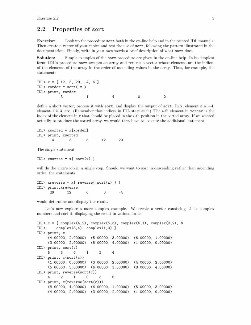
Solution: Simple examples of the sort procedure are given in the on-line help. In its simplestform, IDL’s procedure sort accepts an array and returns a vector whose elements are the indicesof the elements of the array in the order of ascending values in the array. Thus, for example, thestatements
IDL> x = [ 12, 3, 29, -4, 6 ]
IDL> xorder = sort( x )
IDL> print, xorder
3 1 4 0 2
define a short vector, process it with sort, and display the output of sort. In x, element 3 is −4,element 1 is 3, etc. (Remember that indices in IDL start at 0.) The i-th element in xorder is theindex of the element in x that should be placed in the i-th position in the sorted array. If we wantedactually to produce the sorted array, we would then have to execute the additional statement,
IDL> xsorted = x[xorder]
IDL> print, xsorted
-4 3 6 12 29
The single statement,
IDL> xsorted = x[ sort(x) ]
will do the entire job in a single step. Should we want to sort in descending rather than ascendingorder, the statements
IDL> xreverse = x[ reverse( sort(x) ) ]
IDL> print,xreverse
29 12 6 3 -4
would determine and display the result.
Let’s now explore a more complex example. We create a vector consisting of six complexnumbers and sort it, displaying the result in various forms.
IDL> c = [ complex(4,2), complex(5,3), complex(6,1), complex(3,2), $
IDL> complex(8,4), complex(1,0) ]
IDL> print, c
(4.00000, 2.00000) (5.00000, 3.00000) (6.00000, 1.00000)
(3.00000, 2.00000) (8.00000, 4.00000) (1.00000, 0.00000)
IDL> print, sort(c)
5 3 0 1 2 4
IDL> print, c(sort(c))
(1.00000, 0.00000) (3.00000, 2.00000) (4.00000, 2.00000)
(5.00000, 3.00000) (6.00000, 1.00000) (8.00000, 4.00000)
IDL> print, reverse(sort(c))
4 2 1 0 3 5
IDL> print, c(reverse(sort(c)))
(8.00000, 4.00000) (6.00000, 1.00000) (5.00000, 3.00000)
(4.00000, 2.00000) (3.00000, 2.00000) (1.00000, 0.00000)
4 Exercise 2.2
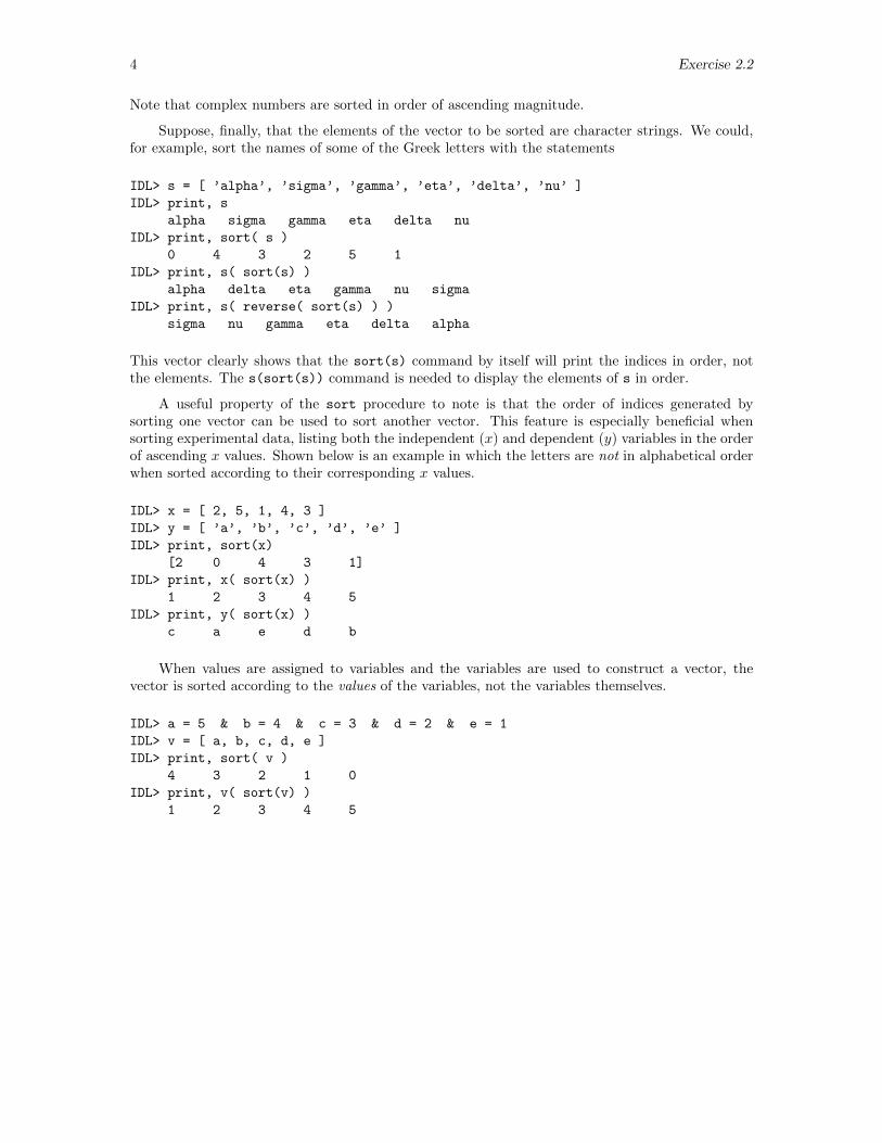
Note that complex numbers are sorted in order of ascending magnitude.
Suppose, finally, that the elements of the vector to be sorted are character strings. We could,for example, sort the names of some of the Greek letters with the statements
IDL> s = [ ’alpha’, ’sigma’, ’gamma’, ’eta’, ’delta’, ’nu’ ]
IDL> print, s
alpha sigma gamma eta delta nu
IDL> print, sort( s )
0 4 3 2 5 1
IDL> print, s( sort(s) )
alpha delta eta gamma nu sigma
IDL> print, s( reverse( sort(s) ) )
sigma nu gamma eta delta alpha
This vector clearly shows that the sort(s) command by itself will print the indices in order, notthe elements. The s(sort(s)) command is needed to display the elements of s in order.
A useful property of the sort procedure to note is that the order of indices generated bysorting one vector can be used to sort another vector. This feature is especially beneficial whensorting experimental data, listing both the independent (x) and dependent (y) variables in the orderof ascending x values. Shown below is an example in which the letters are not in alphabetical orderwhen sorted according to their corresponding x values.
IDL> x = [ 2, 5, 1, 4, 3 ]
IDL> y = [ ’a’, ’b’, ’c’, ’d’, ’e’ ]
IDL> print, sort(x)
[2 0 4 3 1]
IDL> print, x( sort(x) )
1 2 3 4 5
IDL> print, y( sort(x) )
c a e d b
When values are assigned to variables and the variables are used to construct a vector, thevector is sorted according to the values of the variables, not the variables themselves.
IDL> a = 5 & b = 4 & c = 3 & d = 2 & e = 1
IDL> v = [ a, b, c, d, e ]
IDL> print, sort( v )
4 3 2 1 0
IDL> print, v( sort(v) )
1 2 3 4 5
Exercise 2.5 5
2.5 Summing Elements in a Vector
Exercise: (a) Describe and test a sequence of IDL statements that uses a for/do loop toevaluate
∑i ai when the values of ai are supplied as the elements of the vector a. In essence you
will have to initialize a variable to zero and then, in the loop, successively add to that variable eachof the elements ai in turn. (b) Describe and test a sequence of IDL statements that uses the built-infunction total to achieve the same end.
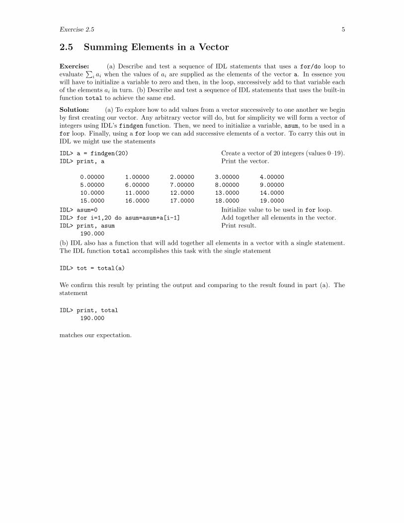
Solution: (a) To explore how to add values from a vector successively to one another we beginby first creating our vector. Any arbitrary vector will do, but for simplicity we will form a vector ofintegers using IDL’s findgen function. Then, we need to initialize a variable, asum, to be used in afor loop. Finally, using a for loop we can add successive elements of a vector. To carry this out inIDL we might use the statements
IDL> a = findgen(20)
IDL> print, a
0.00000 1.00000 2.00000 3.00000 4.00000
5.00000 6.00000 7.00000 8.00000 9.00000
10.0000 11.0000 12.0000 13.0000 14.0000
15.0000 16.0000 17.0000 18.0000 19.0000
Create a vector of 20 integers (values 0–19).Print the vector.
IDL> asum=0
IDL> for i=1,20 do asum=asum+a[i-1]
IDL> print, asum
190.000
Initialize value to be used in for loop.Add together all elements in the vector.Print result.
(b) IDL also has a function that will add together all elements in a vector with a single statement.The IDL function total accomplishes this task with the single statement
IDL> tot = total(a)
We confirm this result by printing the output and comparing to the result found in part (a). Thestatement
IDL> print, total
190.000
matches our expectation.
6 Exercise 2.6
2.6 Evaluating a Cross Product
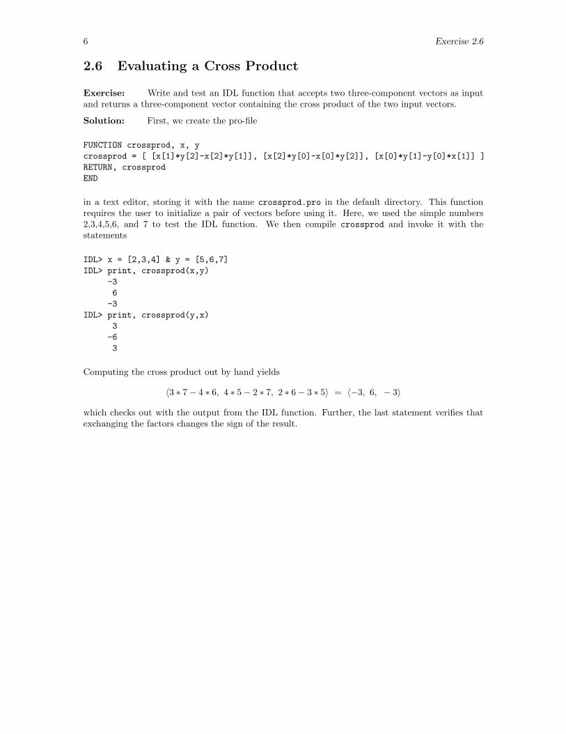
Exercise: Write and test an IDL function that accepts two three-component vectors as inputand returns a three-component vector containing the cross product of the two input vectors.
Solution: First, we create the pro-file
FUNCTION crossprod, x, y
crossprod = [ [x[1]*y[2]-x[2]*y[1]], [x[2]*y[0]-x[0]*y[2]], [x[0]*y[1]-y[0]*x[1]] ]
RETURN, crossprod
END
in a text editor, storing it with the name crossprod.pro in the default directory. This functionrequires the user to initialize a pair of vectors before using it. Here, we used the simple numbers2,3,4,5,6, and 7 to test the IDL function. We then compile crossprod and invoke it with thestatements
IDL> x = [2,3,4] & y = [5,6,7]
IDL> print, crossprod(x,y)
-3
6
-3
IDL> print, crossprod(y,x)
3
-6
3
Computing the cross product out by hand yields
〈3 ∗ 7− 4 ∗ 6, 4 ∗ 5− 2 ∗ 7, 2 ∗ 6− 3 ∗ 5〉 = 〈−3, 6, − 3〉
which checks out with the output from the IDL function. Further, the last statement verifies thatexchanging the factors changes the sign of the result.
Exercise 2.8 7
2.8 Eigenvectors/Values in a Single Matrix
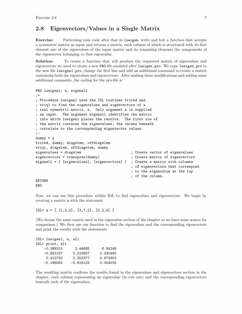
Exercise: Patterning your code after that in lueigen, write and test a function that acceptsa symmetric matrix as input and returns a matrix, each column of which is structured with its firstelement one of the eigenvalues of the input matrix and its remaining elements the components ofthe eigenvector belonging to that eigenvalue.
Solution: To create a function that will produce the requested matrix of eigenvalues andeigenvectors we need to create a new PRO file modeled after lueigen.pro. We copy lueigen.pro tothe new file lueigen1.pro, change the first line and add an additional command to create a matrixcontaining both the eigenvalues and eigenvectors. After making these modifications and adding someadditional comments, the coding for the pro-file is
PRO lueigen1, a, eigenall
;+
; Procedure lueigen1 uses the IDL routines trired and
; triq1 to find the eigenvalues and eigenvectors of a
; real symmetric matrix, a. Only argument a is supplied
; as input. The argument eigenall identifies the matrix
; into which lueigen1 places the results. The first row of
; the matrix contains the eigenvalues, the values beneath
; correlate to the corresponding eigenvector values.
;-
dummy = a
trired, dummy, diagelem, offdiagelem
triql, diagelem, offdiagelem, dummy
eigenvalues = diagelem ; Create vector of eigenvalues
eigenvectors = transpose(dummy) ; Create matrix of eigenvectors
eigenall = [ [eigenvalues], [eigenvectors] ] ; Create a matrix with columns
; of eigenvectors that correspond
; to the eigenvalue at the top
; of the column.
RETURN
END
Now, we can use this procedure within IDL to find eigenvalues and eigenvectors. We begin bycreating a matrix a with the statement
IDL> a = [ [1,3,0], [3,7,2], [0,2,4] ]
(We choose the same matrix used in the eigenvalue section of the chapter so we have some source forcomparison.) We then use our function to find the eigenvalues and the corresponding eigenvectorsand print the results with the statements
IDL> lueigen1, a, all
IDL> print, all
-0.389315 3.44685 8.94246
-0.891227 0.310657 0.330465
0.412732 0.253377 0.874902
-0.188062 -0.916129 0.354035
The resulting matrix confirms the results found in the eigenvalues and eigenvectors section in thechapter, each column representing an eigenvalue (in row one) and the corresponding eigenvectorsbeneath each of the eigenvalues.
8 Exercise 2.9
2.9 Finding/Plotting Eigenvalues/Vectors
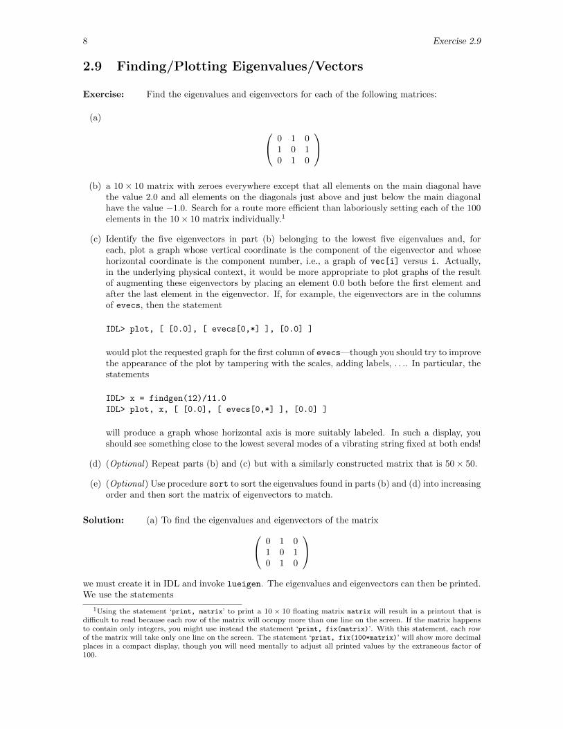
Exercise: Find the eigenvalues and eigenvectors for each of the following matrices:
(a) 0 1 01 0 10 1 0
(b) a 10 × 10 matrix with zeroes everywhere except that all elements on the main diagonal have
the value 2.0 and all elements on the diagonals just above and just below the main diagonalhave the value −1.0. Search for a route more efficient than laboriously setting each of the 100elements in the 10× 10 matrix individually.1
(c) Identify the five eigenvectors in part (b) belonging to the lowest five eigenvalues and, foreach, plot a graph whose vertical coordinate is the component of the eigenvector and whosehorizontal coordinate is the component number, i.e., a graph of vec[i] versus i. Actually,in the underlying physical context, it would be more appropriate to plot graphs of the resultof augmenting these eigenvectors by placing an element 0.0 both before the first element andafter the last element in the eigenvector. If, for example, the eigenvectors are in the columnsof evecs, then the statement
IDL> plot, [ [0.0], [ evecs[0,*] ], [0.0] ]
would plot the requested graph for the first column of evecs—though you should try to improvethe appearance of the plot by tampering with the scales, adding labels, . . .. In particular, thestatements
IDL> x = findgen(12)/11.0
IDL> plot, x, [ [0.0], [ evecs[0,*] ], [0.0] ]
will produce a graph whose horizontal axis is more suitably labeled. In such a display, youshould see something close to the lowest several modes of a vibrating string fixed at both ends!
(d) (Optional) Repeat parts (b) and (c) but with a similarly constructed matrix that is 50× 50.
(e) (Optional) Use procedure sort to sort the eigenvalues found in parts (b) and (d) into increasingorder and then sort the matrix of eigenvectors to match.
Solution: (a) To find the eigenvalues and eigenvectors of the matrix 0 1 01 0 10 1 0
we must create it in IDL and invoke lueigen. The eigenvalues and eigenvectors can then be printed.We use the statements
1Using the statement ‘print, matrix’ to print a 10 × 10 floating matrix matrix will result in a printout that isdifficult to read because each row of the matrix will occupy more than one line on the screen. If the matrix happensto contain only integers, you might use instead the statement ‘print, fix(matrix)’. With this statement, each rowof the matrix will take only one line on the screen. The statement ‘print, fix(100*matrix)’ will show more decimalplaces in a compact display, though you will need mentally to adjust all printed values by the extraneous factor of100.
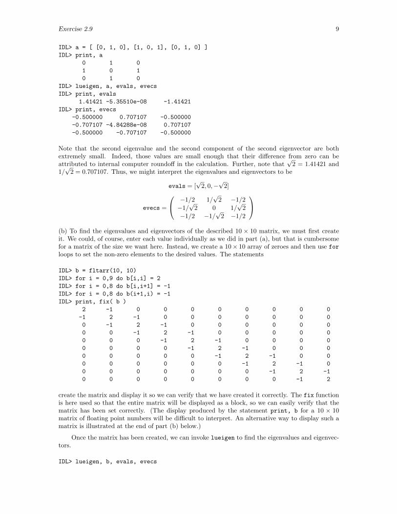
Exercise 2.9 9
IDL> a = [ [0, 1, 0], [1, 0, 1], [0, 1, 0] ]
IDL> print, a
0 1 0
1 0 1
0 1 0
IDL> lueigen, a, evals, evecs
IDL> print, evals
1.41421 -5.35510e-08 -1.41421
IDL> print, evecs
-0.500000 0.707107 -0.500000
-0.707107 -4.84288e-08 0.707107
-0.500000 -0.707107 -0.500000
Note that the second eigenvalue and the second component of the second eigenvector are bothextremely small. Indeed, those values are small enough that their difference from zero can beattributed to internal computer roundoff in the calculation. Further, note that
√2 = 1.41421 and
1/√
2 = 0.707107. Thus, we might interpret the eigenvalues and eigenvectors to be
evals = [√
2, 0,−√
2]
evecs =
−1/2 1/√
2 −1/2
−1/√
2 0 1/√
2
−1/2 −1/√
2 −1/2
(b) To find the eigenvalues and eigenvectors of the described 10 × 10 matrix, we must first createit. We could, of course, enter each value individually as we did in part (a), but that is cumbersomefor a matrix of the size we want here. Instead, we create a 10× 10 array of zeroes and then use for
loops to set the non-zero elements to the desired values. The statements
IDL> b = fltarr(10, 10)
IDL> for i = 0,9 do b[i,i] = 2
IDL> for i = 0,8 do b[i,i+1] = -1
IDL> for i = 0,8 do b(i+1,i) = -1
IDL> print, fix( b )
2 -1 0 0 0 0 0 0 0 0
-1 2 -1 0 0 0 0 0 0 0
0 -1 2 -1 0 0 0 0 0 0
0 0 -1 2 -1 0 0 0 0 0
0 0 0 -1 2 -1 0 0 0 0
0 0 0 0 -1 2 -1 0 0 0
0 0 0 0 0 -1 2 -1 0 0
0 0 0 0 0 0 -1 2 -1 0
0 0 0 0 0 0 0 -1 2 -1
0 0 0 0 0 0 0 0 -1 2
create the matrix and display it so we can verify that we have created it correctly. The fix functionis here used so that the entire matrix will be displayed as a block, so we can easily verify that thematrix has been set correctly. (The display produced by the statement print, b for a 10 × 10matrix of floating point numbers will be difficult to interpret. An alternative way to display such amatrix is illustrated at the end of part (b) below.)
Once the matrix has been created, we can invoke lueigen to find the eigenvalues and eigenvec-tors.
IDL> lueigen, b, evals, evecs
10 Exercise 2.9
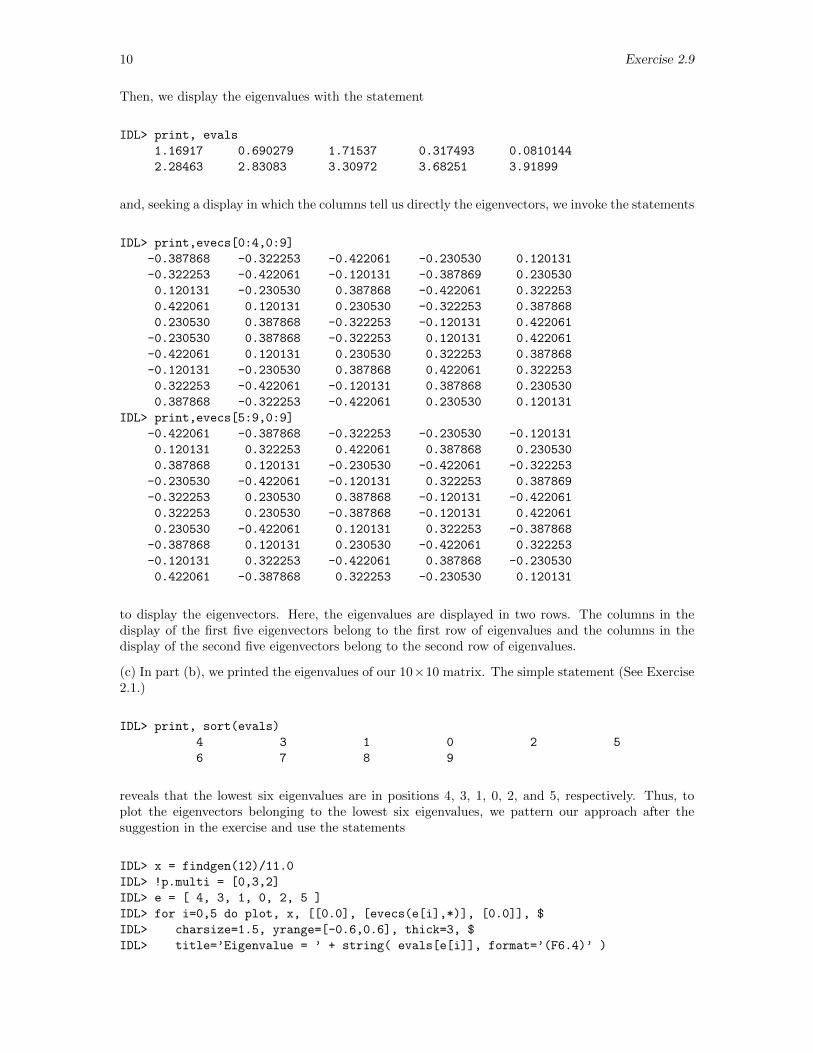
Then, we display the eigenvalues with the statement
IDL> print, evals
1.16917 0.690279 1.71537 0.317493 0.0810144
2.28463 2.83083 3.30972 3.68251 3.91899
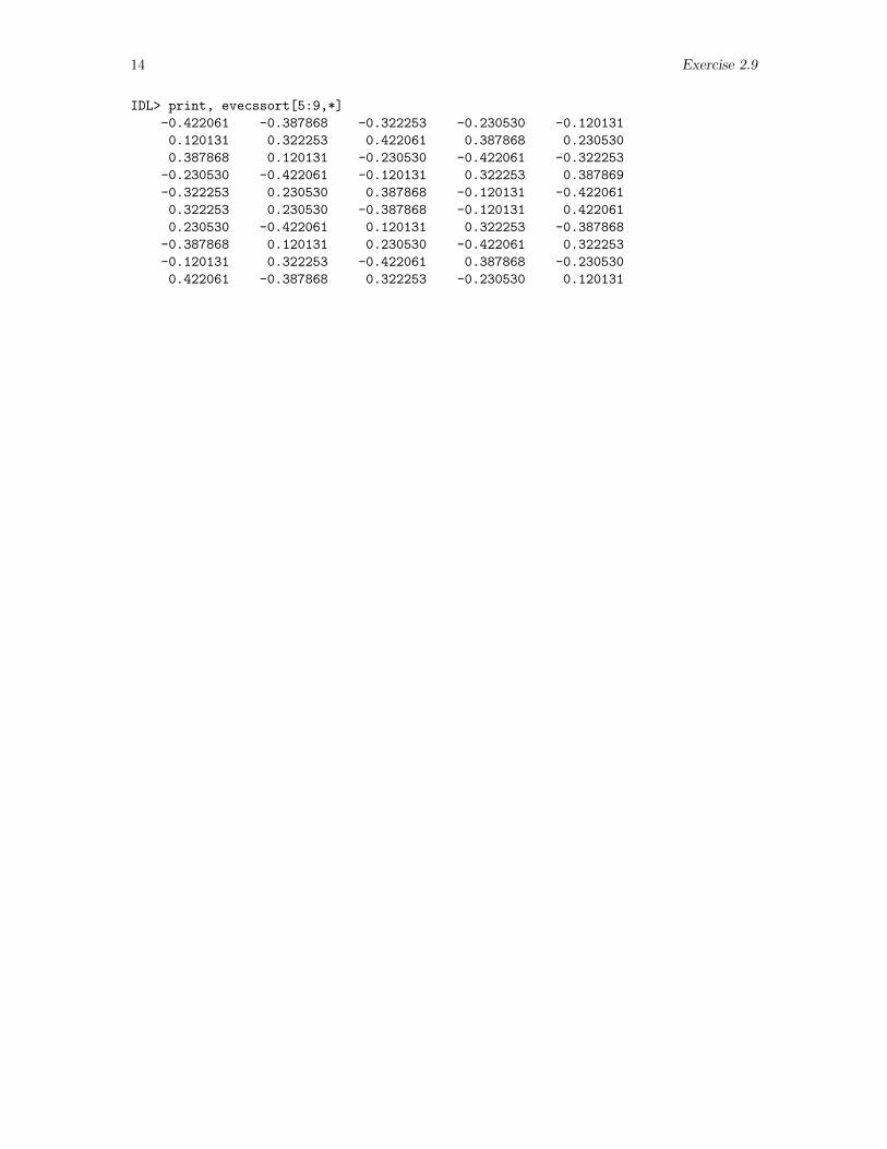
and, seeking a display in which the columns tell us directly the eigenvectors, we invoke the statements
IDL> print,evecs[0:4,0:9]
-0.387868 -0.322253 -0.422061 -0.230530 0.120131
-0.322253 -0.422061 -0.120131 -0.387869 0.230530
0.120131 -0.230530 0.387868 -0.422061 0.322253
0.422061 0.120131 0.230530 -0.322253 0.387868
0.230530 0.387868 -0.322253 -0.120131 0.422061
-0.230530 0.387868 -0.322253 0.120131 0.422061
-0.422061 0.120131 0.230530 0.322253 0.387868
-0.120131 -0.230530 0.387868 0.422061 0.322253
0.322253 -0.422061 -0.120131 0.387868 0.230530
0.387868 -0.322253 -0.422061 0.230530 0.120131
IDL> print,evecs[5:9,0:9]
-0.422061 -0.387868 -0.322253 -0.230530 -0.120131
0.120131 0.322253 0.422061 0.387868 0.230530
0.387868 0.120131 -0.230530 -0.422061 -0.322253
-0.230530 -0.422061 -0.120131 0.322253 0.387869
-0.322253 0.230530 0.387868 -0.120131 -0.422061
0.322253 0.230530 -0.387868 -0.120131 0.422061
0.230530 -0.422061 0.120131 0.322253 -0.387868
-0.387868 0.120131 0.230530 -0.422061 0.322253
-0.120131 0.322253 -0.422061 0.387868 -0.230530
0.422061 -0.387868 0.322253 -0.230530 0.120131
to display the eigenvectors. Here, the eigenvalues are displayed in two rows. The columns in thedisplay of the first five eigenvectors belong to the first row of eigenvalues and the columns in thedisplay of the second five eigenvectors belong to the second row of eigenvalues.
(c) In part (b), we printed the eigenvalues of our 10×10 matrix. The simple statement (See Exercise2.1.)
IDL> print, sort(evals)
4 3 1 0 2 5
6 7 8 9
reveals that the lowest six eigenvalues are in positions 4, 3, 1, 0, 2, and 5, respectively. Thus, toplot the eigenvectors belonging to the lowest six eigenvalues, we pattern our approach after thesuggestion in the exercise and use the statements
IDL> x = findgen(12)/11.0
IDL> !p.multi = [0,3,2]
IDL> e = [ 4, 3, 1, 0, 2, 5 ]
IDL> for i=0,5 do plot, x, [[0.0], [evecs(e[i],*)], [0.0]], $
IDL> charsize=1.5, yrange=[-0.6,0.6], thick=3, $
IDL> title=’Eigenvalue = ’ + string( evals[e[i]], format=’(F6.4)’ )
Exercise 2.9 11
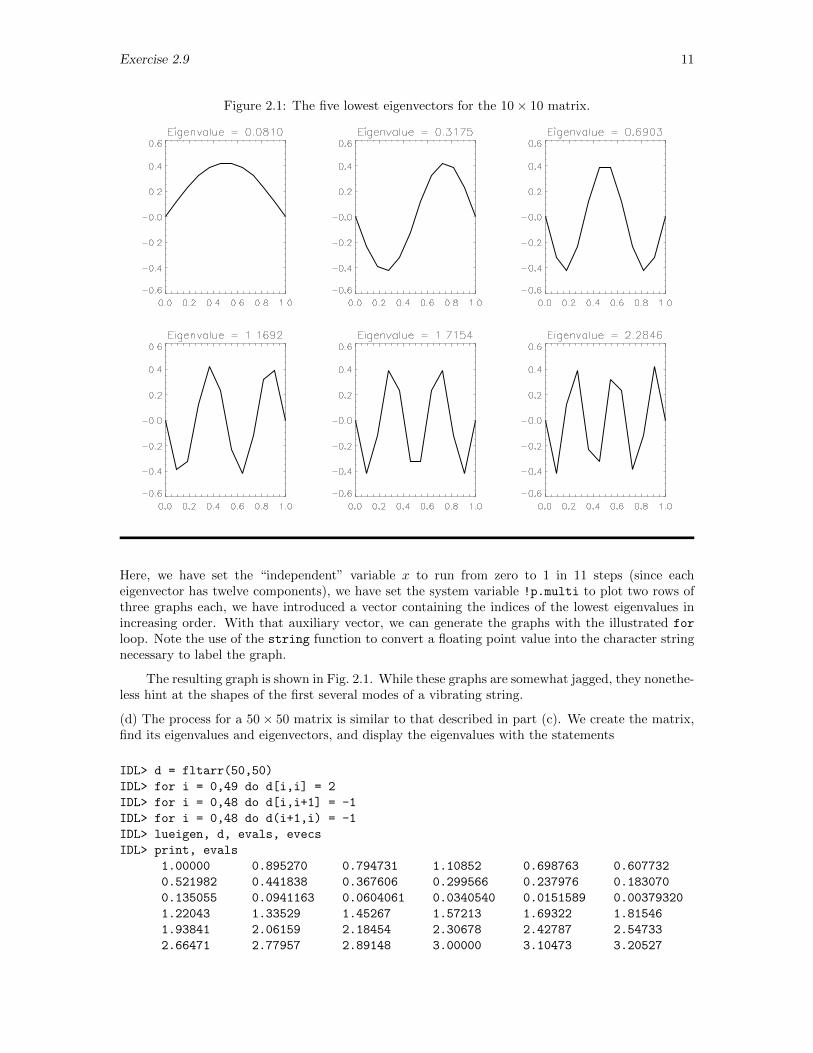
Figure 2.1: The five lowest eigenvectors for the 10× 10 matrix.
Here, we have set the “independent” variable x to run from zero to 1 in 11 steps (since eacheigenvector has twelve components), we have set the system variable !p.multi to plot two rows ofthree graphs each, we have introduced a vector containing the indices of the lowest eigenvalues inincreasing order. With that auxiliary vector, we can generate the graphs with the illustrated for
loop. Note the use of the string function to convert a floating point value into the character stringnecessary to label the graph.
The resulting graph is shown in Fig. 2.1. While these graphs are somewhat jagged, they nonethe-less hint at the shapes of the first several modes of a vibrating string.
(d) The process for a 50× 50 matrix is similar to that described in part (c). We create the matrix,find its eigenvalues and eigenvectors, and display the eigenvalues with the statements
IDL> d = fltarr(50,50)
IDL> for i = 0,49 do d[i,i] = 2
IDL> for i = 0,48 do d[i,i+1] = -1
IDL> for i = 0,48 do d(i+1,i) = -1
IDL> lueigen, d, evals, evecs
IDL> print, evals
1.00000 0.895270 0.794731 1.10852 0.698763 0.607732
0.521982 0.441838 0.367606 0.299566 0.237976 0.183070
0.135055 0.0941163 0.0604061 0.0340540 0.0151589 0.00379320
1.22043 1.33529 1.45267 1.57213 1.69322 1.81546
1.93841 2.06159 2.18454 2.30678 2.42787 2.54733
2.66471 2.77957 2.89148 3.00000 3.10473 3.20527
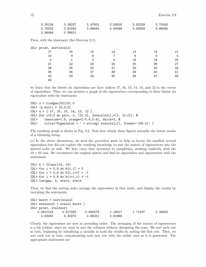
12 Exercise 2.9
3.30124 3.39227 3.47802 3.55816 3.63239 3.70043
3.76202 3.81693 3.86494 3.90588 3.93959 3.96595
3.98484 3.99621
Then, with the statement (See Exercise 2.1),
IDL> print, sort(evals)
17 16 15 14 13 12 11
10 9 8 7 6 5 4
2 1 0 3 18 19 20
21 22 23 24 25 26 27
28 29 30 31 32 33 34
35 36 37 38 39 40 41
42 43 44 45 46 47 48
49
we learn that the lowest six eigenvalues are have indices 17, 16, 15, 14, 13, and 12 in the vectorof eigenvalues. Thus, we can produce a graph of the eigenvectors corresponding to these lowest sixeigenvalues with the statements
IDL> x = findgen(52)/51.0
IDL> !p.multi = [0,3,2]
IDL> e = [ 17, 16, 15, 14, 13, 12 ]
IDL> for i=0,5 do plot, x, [[0.0], [evecs(e[i],*)], [0.0]], $
IDL> charsize=1.5, yrange=[-0.4,0.4], thick=3, $
IDL> title=’Eigenvalue = ’ + string( evals[e[i]], format=’(F6.4)’ )
The resulting graph is shown in Fig. 2.2. Note how closely these figures resemble the lowest modesof a vibrating string.
(e) In the above discussions, we used the procedure sort to help us locate the smallest severaleigenvalues but did not exploit the resulting knowledge to sort the matrix of eigenvectors into thedesired order as well. We here carry that operation to completion, working explicitly with the10× 10 case. We reconstruct the original matrix and find its eigenvalues and eigenvectors with thestatements
IDL> b = fltarr(10, 10)
IDL> for i = 0,9 do b[i,i] = 2
IDL> for i = 0,8 do b[i,i+1] = -1
IDL> for i = 0,8 do b(i+1,i) = -1
IDL> lueigen, b, evals, evecs
Then, we find the sorting order arrange the eigenvalues in that order, and display the results byexecuting the statements
IDL> bsort = sort(evals)
IDL> evalssort = evals[ bsort ]
IDL> print, evalssort
0.0810143 0.317493 0.690279 1.16917 1.71537 2.28463
2.83083 3.30972 3.68251 3.91899
Clearly, the eigenvalues are now in ascending order. The arranging of the matrix of eigenvectorsis a bit trickier, since we want to sort the columns without disrupting the rows. We sort each rowin turn, beginning by initializing a variable to hold the results by sorting the first row. Then, wesort each row in turn, concatenating each new row with the earlier ones as it is generated. Theappropriate statements are
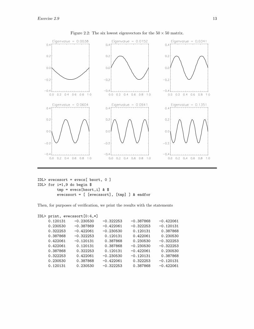
Exercise 2.9 13
Figure 2.2: The six lowest eigenvectors for the 50× 50 matrix.
IDL> evecssort = evecs[ bsort, 0 ]
IDL> for i=1,9 do begin $
tmp = evecs[bsort,i] & $
evecssort = [ [evecssort], [tmp] ] & endfor
Then, for purposes of verification, we print the results with the statements
IDL> print, evecssort[0:4,*]
0.120131 -0.230530 -0.322253 -0.387868 -0.422061
0.230530 -0.387869 -0.422061 -0.322253 -0.120131
0.322253 -0.422061 -0.230530 0.120131 0.387868
0.387868 -0.322253 0.120131 0.422061 0.230530
0.422061 -0.120131 0.387868 0.230530 -0.322253
0.422061 0.120131 0.387868 -0.230530 -0.322253
0.387868 0.322253 0.120131 -0.422061 0.230530
0.322253 0.422061 -0.230530 -0.120131 0.387868
0.230530 0.387868 -0.422061 0.322253 -0.120131
0.120131 0.230530 -0.322253 0.387868 -0.422061
14 Exercise 2.9
IDL> print, evecssort[5:9,*]
-0.422061 -0.387868 -0.322253 -0.230530 -0.120131
0.120131 0.322253 0.422061 0.387868 0.230530
0.387868 0.120131 -0.230530 -0.422061 -0.322253
-0.230530 -0.422061 -0.120131 0.322253 0.387869
-0.322253 0.230530 0.387868 -0.120131 -0.422061
0.322253 0.230530 -0.387868 -0.120131 0.422061
0.230530 -0.422061 0.120131 0.322253 -0.387868
-0.387868 0.120131 0.230530 -0.422061 0.322253
-0.120131 0.322253 -0.422061 0.387868 -0.230530
0.422061 -0.387868 0.322253 -0.230530 0.120131
Exercise 2.10 15
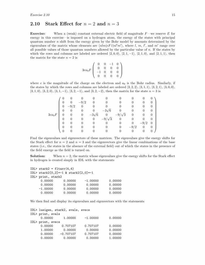
2.10 Stark Effect for n = 2 and n = 3
Exercise: When a (weak) constant external electric field of magnitude F—we reserve E forenergy in this exercise—is imposed on a hydrogen atom, the energy of the states with principalquantum number n shift from the energy given by the Bohr model by amounts determined by theeigenvalues of the matrix whose elements are 〈nlm|eF z|nl′m′〉, where l, m, l′, and m′ range overall possible values of those quantum numbers allowed by the particular value of n. If the states bywhich the rows and columns are labeled are ordered |2, 0, 0〉, |2, 1,−1〉, |2, 1, 0〉, and |2, 1, 1〉, thenthe matrix for the state n = 2 is
3ea0F
0 0 −1 00 0 0 0−1 0 0 00 0 0 0
where e is the magnitude of the charge on the electron and a0 is the Bohr radius. Similarly, ifthe states by which the rows and columns are labeled are ordered |3, 2, 2〉, |3, 1, 1〉, |3, 2, 1〉, |3, 0, 0〉,|3, 1, 0〉, |3, 2, 0〉, |3, 1,−1〉, |3, 2,−1〉, and |3, 2,−2〉, then the matrix for the state n = 3 is
3ea0F
0 0 0 0 0 0 0 0 00 0 −9/2 0 0 0 0 0 00 −9/2 0 0 0 0 0 0 0
0 0 0 0 −3√
6 0 0 0 0
0 0 0 −3√
6 0 −9/√
3 0 0 0
0 0 0 0 −9/√
3 0 0 0 00 0 0 0 0 0 0 −9/2 00 0 0 0 0 0 −9/2 0 00 0 0 0 0 0 0 0 0
Find the eigenvalues and eigenvectors of these matrices. The eigenvalues give the energy shifts forthe Stark effect for n = 2 and n = 3 and the eigenvectors give the linear combinations of the basestates (i.e., the states in the absence of the external field) out of which the states in the presence ofthe field emerge as the field is turned on.
Solution: When n = 2, the matrix whose eigenvalues give the energy shifts for the Stark effectin hydrogen is created simply in IDL with the statements
IDL> stark2 = fltarr(4,4)
IDL> stark2[0,2]=-1 & stark2[2,0]=-1
IDL> print, stark2
0.00000 0.00000 -1.00000 0.00000
0.00000 0.00000 0.00000 0.00000
-1.00000 0.00000 0.00000 0.00000
0.00000 0.00000 0.00000 0.00000
We then find and display its eigenvalues and eigenvectors with the statements
IDL> lueigen, stark2, evals, evecs
IDL> print, evals
0.00000 1.00000 -1.00000 0.00000
IDL> print, evecs
0.00000 0.707107 0.707107 0.00000
1.00000 0.00000 0.00000 0.00000
0.00000 -0.707107 0.707107 0.00000
0.00000 0.00000 0.00000 1.00000
16 Exercise 2.10
(Note, incidentally, that 0.707107 = 1/√
2.) Evidently, two states (|2, 0,−1〉, and |2, 1, 1〉) are notaffected by the perturbation and two states,
1√2
(|2, 0, 0〉 ± |2, 1, 0〉
)are shifted, one up in energy by one unit (i.e., by 3ea0F ) and the other down by one unit. Thedegeneracy is partly but not completely lifted by the application of the perturbation.
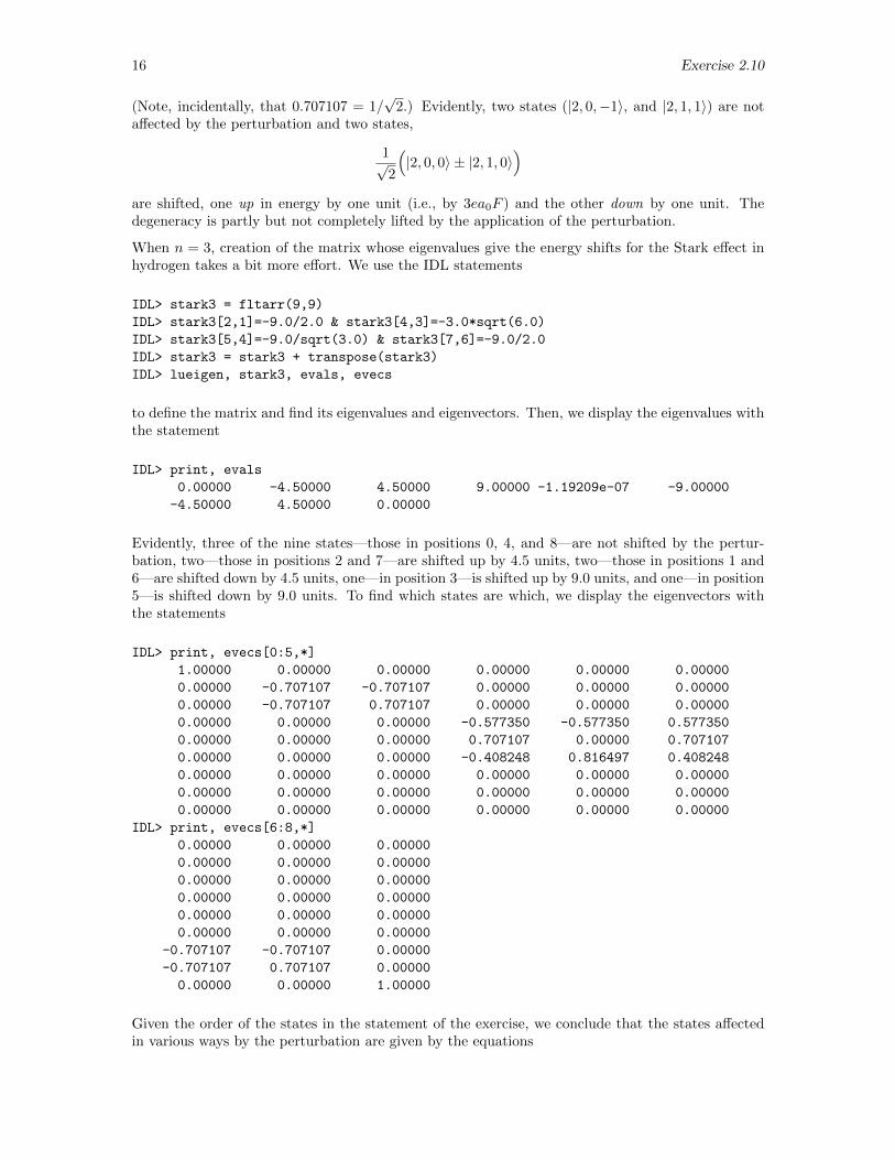
When n = 3, creation of the matrix whose eigenvalues give the energy shifts for the Stark effect inhydrogen takes a bit more effort. We use the IDL statements
IDL> stark3 = fltarr(9,9)
IDL> stark3[2,1]=-9.0/2.0 & stark3[4,3]=-3.0*sqrt(6.0)
IDL> stark3[5,4]=-9.0/sqrt(3.0) & stark3[7,6]=-9.0/2.0
IDL> stark3 = stark3 + transpose(stark3)
IDL> lueigen, stark3, evals, evecs
to define the matrix and find its eigenvalues and eigenvectors. Then, we display the eigenvalues withthe statement
IDL> print, evals
0.00000 -4.50000 4.50000 9.00000 -1.19209e-07 -9.00000
-4.50000 4.50000 0.00000
Evidently, three of the nine states—those in positions 0, 4, and 8—are not shifted by the pertur-bation, two—those in positions 2 and 7—are shifted up by 4.5 units, two—those in positions 1 and6—are shifted down by 4.5 units, one—in position 3—is shifted up by 9.0 units, and one—in position5—is shifted down by 9.0 units. To find which states are which, we display the eigenvectors withthe statements
IDL> print, evecs[0:5,*]
1.00000 0.00000 0.00000 0.00000 0.00000 0.00000
0.00000 -0.707107 -0.707107 0.00000 0.00000 0.00000
0.00000 -0.707107 0.707107 0.00000 0.00000 0.00000
0.00000 0.00000 0.00000 -0.577350 -0.577350 0.577350
0.00000 0.00000 0.00000 0.707107 0.00000 0.707107
0.00000 0.00000 0.00000 -0.408248 0.816497 0.408248
0.00000 0.00000 0.00000 0.00000 0.00000 0.00000
0.00000 0.00000 0.00000 0.00000 0.00000 0.00000
0.00000 0.00000 0.00000 0.00000 0.00000 0.00000
IDL> print, evecs[6:8,*]
0.00000 0.00000 0.00000
0.00000 0.00000 0.00000
0.00000 0.00000 0.00000
0.00000 0.00000 0.00000
0.00000 0.00000 0.00000
0.00000 0.00000 0.00000
-0.707107 -0.707107 0.00000
-0.707107 0.707107 0.00000
0.00000 0.00000 1.00000
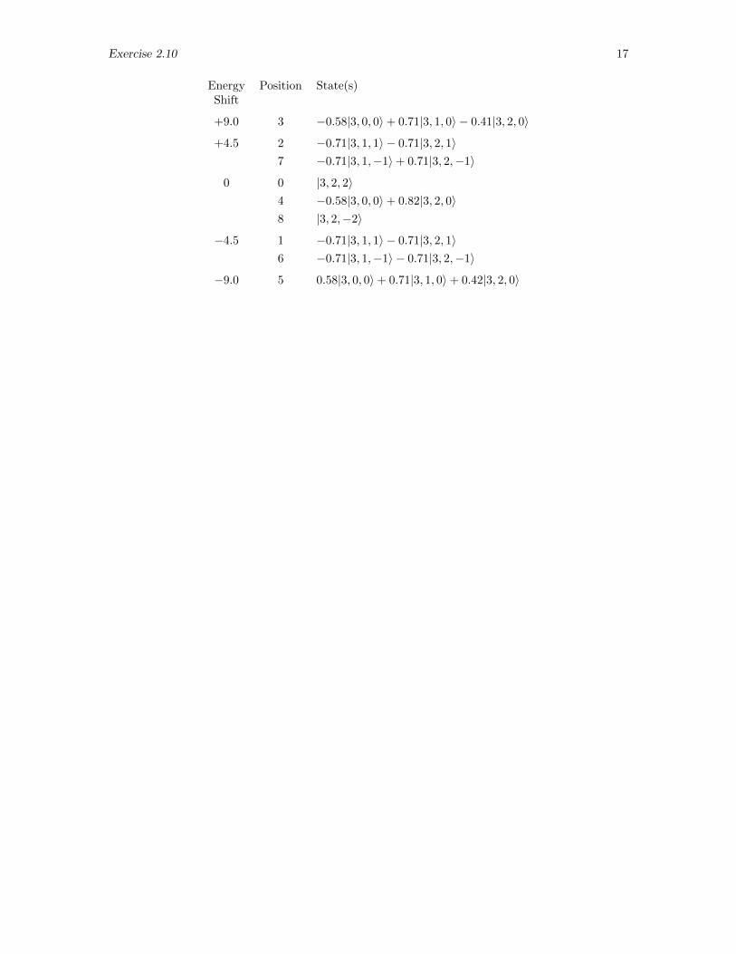
Given the order of the states in the statement of the exercise, we conclude that the states affectedin various ways by the perturbation are given by the equations
Exercise 2.10 17
Energy Position State(s)Shift
+9.0 3 −0.58|3, 0, 0〉+ 0.71|3, 1, 0〉 − 0.41|3, 2, 0〉
+4.5 2 −0.71|3, 1, 1〉 − 0.71|3, 2, 1〉7 −0.71|3, 1,−1〉+ 0.71|3, 2,−1〉
0 0 |3, 2, 2〉4 −0.58|3, 0, 0〉+ 0.82|3, 2, 0〉8 |3, 2,−2〉
−4.5 1 −0.71|3, 1, 1〉 − 0.71|3, 2, 1〉6 −0.71|3, 1,−1〉 − 0.71|3, 2,−1〉
−9.0 5 0.58|3, 0, 0〉+ 0.71|3, 1, 0〉+ 0.42|3, 2, 0〉
18 Exercise 2.11
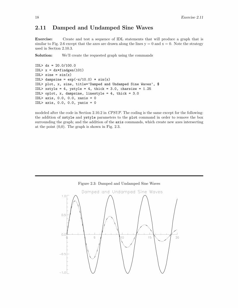
2.11 Damped and Undamped Sine Waves
Exercise: Create and test a sequence of IDL statements that will produce a graph that issimilar to Fig. 2.6 except that the axes are drawn along the lines y = 0 and x = 0. Note the strategyused in Section 2.10.3.
Solution: We’ll create the requested graph using the commands
IDL> dx = 20.0/100.0
IDL> x = dx*findgen(101)
IDL> sine = sin(x)
IDL> dampsine = exp(-x/10.0) * sin(x)
IDL> plot, x, sine, title=’Damped and Undamped Sine Waves’, $
IDL> xstyle = 4, ystyle = 4, thick = 3.0, charsize = 1.25
IDL> oplot, x, dampsine, linestyle = 4, thick = 3.0
IDL> axis, 0.0, 0.0, xaxis = 0
IDL> axis, 0.0, 0.0, yaxis = 0
modeled after the code in Section 2.10.2 in CPSUP. The coding is the same except for the following:the addition of xstyle and ystyle parameters to the plot command in order to remove the boxsurrounding the graph; and the addition of the axis commands, which create new axes intersectingat the point (0,0). The graph is shown in Fig. 2.3.
Figure 2.3: Damped and Undamped Sine Waves
Exercise 2.13 19
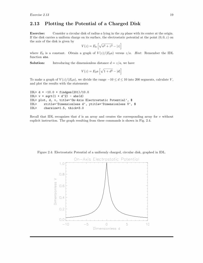
2.13 Plotting the Potential of a Charged Disk
Exercise: Consider a circular disk of radius a lying in the xy plane with its center at the origin.If the disk carries a uniform charge on its surface, the electrostatic potential at the point (0, 0, z) onthe axis of the disk is given by
V (z) = E0
[√a2 + z2 − |z|
]where E0 is a constant. Obtain a graph of V (z)/(E0a) versus z/a. Hint : Remember the IDLfunction abs.
Solution: Introducing the dimensionless distance d = z/a, we have
V (z) = E0a[√
1 + d2 − |d|]
To make a graph of V (z)/(E0a), we divide the range −10 ≤ d ≤ 10 into 200 segments, calculate V ,and plot the results with the statements
IDL> d = -10.0 + findgen(201)/10.0
IDL> v = sqrt(1 + d^2) - abs(d)
IDL> plot, d, v, title=’On-Axis Electrostatic Potential’, $
IDL> xtitle=’Dimensionless d’, ytitle=’Dimensionless V’, $
IDL> charsize=1.5, thick=3.0
Recall that IDL recognizes that d is an array and creates the corresponding array for v withoutexplicit instruction. The graph resulting from these commands is shown in Fig. 2.4.
Figure 2.4: Electrostatic Potential of a uniformly charged, circular disk, graphed in IDL.
20 Exercise 2.14
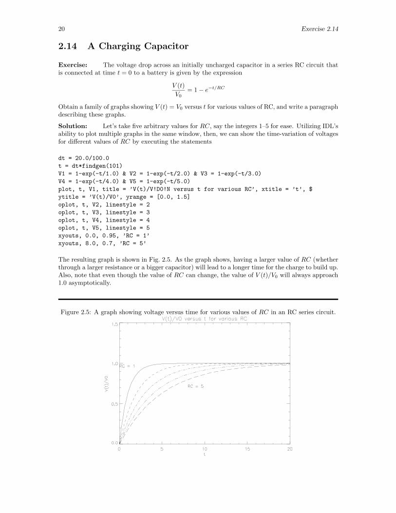
2.14 A Charging Capacitor
Exercise: The voltage drop across an initially uncharged capacitor in a series RC circuit thatis connected at time t = 0 to a battery is given by the expression
V (t)
V0= 1− e−t/RC
Obtain a family of graphs showing V (t) = V0 versus t for various values of RC, and write a paragraphdescribing these graphs.
Solution: Let’s take five arbitrary values for RC, say the integers 1–5 for ease. Utilizing IDL’sability to plot multiple graphs in the same window, then, we can show the time-variation of voltagesfor different values of RC by executing the statements
dt = 20.0/100.0
t = dt*findgen(101)
V1 = 1-exp(-t/1.0) & V2 = 1-exp(-t/2.0) & V3 = 1-exp(-t/3.0)
V4 = 1-exp(-t/4.0) & V5 = 1-exp(-t/5.0)
plot, t, V1, title = ’V(t)/V!D0!N versus t for various RC’, xtitle = ’t’, $
ytitle = ’V(t)/V0’, yrange = [0.0, 1.5]
oplot, t, V2, linestyle = 2
oplot, t, V3, linestyle = 3
oplot, t, V4, linestyle = 4
oplot, t, V5, linestyle = 5
xyouts, 0.0, 0.95, ’RC = 1’
xyouts, 8.0, 0.7, ’RC = 5’
The resulting graph is shown in Fig. 2.5. As the graph shows, having a larger value of RC (whetherthrough a larger resistance or a bigger capacitor) will lead to a longer time for the charge to build up.Also, note that even though the value of RC can change, the value of V (t)/V0 will always approach1.0 asymptotically.
Figure 2.5: A graph showing voltage versus time for various values of RC in an RC series circuit.

Exercise 2.15 21
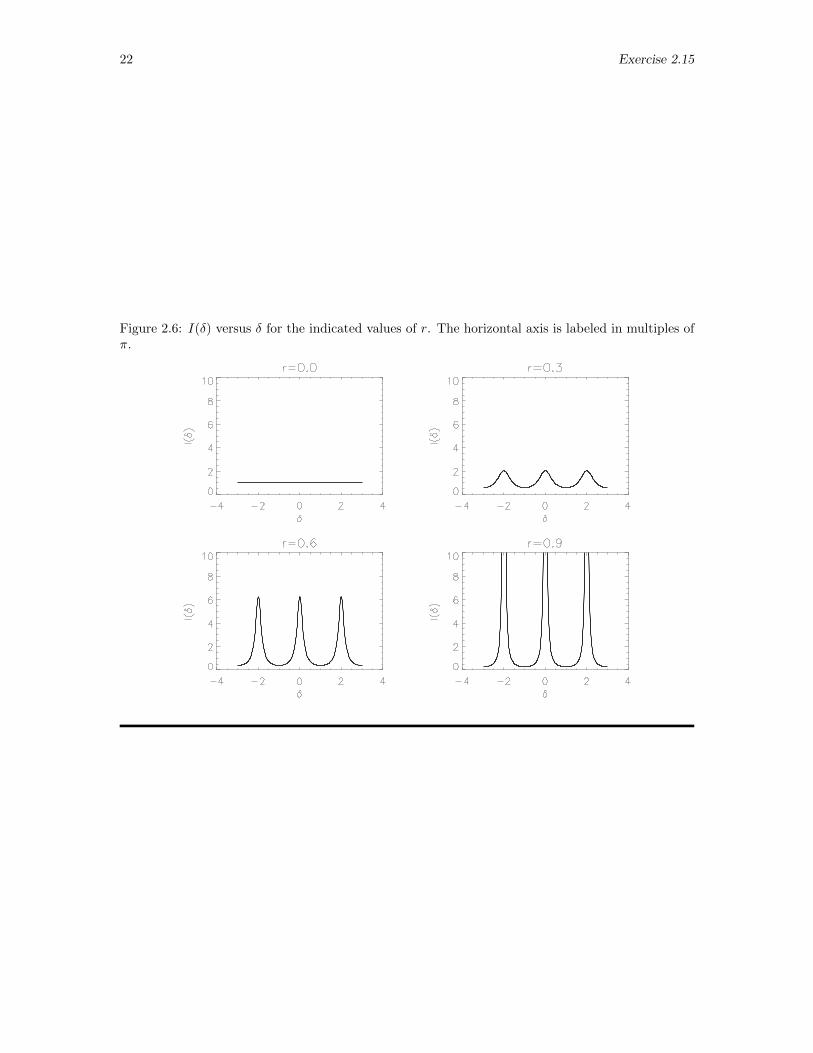
2.15 Plotting the Output of a Fabry-Perot Interferometer
Exercise: In a Fabry-Perot interferometer, a very large number of waves, each out of phasewith the previous one by an amount δ and reduced in amplitude by a factor r, 0 ≤ r < 1, interfere.The resulting intensity is proportional to the expression
I(δ) =1
1− 2r cos δ + r2
Obtain graphs of I(δ) versus δ over the interval −3π ≤ δ ≤ 3π for various values of r, and write aparagraph describing these graphs.
Solution: To evaluate the expression
I(δ) =1
1− 2r cos δ + r2
we first need to create a vector of values of δ. We elect to evaluate the function over the interval3π ≤ δ ≤ 3π and then to display it with the horizontal axis labeled in multiples of π. Thus, we startwith the statement
IDL> del = -3.0 + 6.0*findgen(401)/400.0
IDL> delta = !pi*del
Then, we evaluate the function at selected values of r with the statements
IDL> r = 0.0 & I0 = 1.0 / ( 1.0 - 2.0*r*cos(delta) + r^2 )
IDL> r = 0.3 & I3 = 1.0 / ( 1.0 - 2.0*r*cos(delta) + r^2 )
IDL> r = 0.6 & I6 = 1.0 / ( 1.0 - 2.0*r*cos(delta) + r^2 )
IDL> r = 0.9 & I9 = 1.0 / ( 1.0 - 2.0*r*cos(delta) + r^2 )
Finally, we plot these four relationships with the statements
IDL> !p.multi=[0,2,2] & !x.range=[-3.0,3.0] & !y.range=[0.0,10.0]
IDL> plot, del, I0, thick=3, xtitle=’!4d!3’, ytitle=’I(!4d!3)’, title=’r=0.0’
IDL> plot, del, I3, thick=3, xtitle=’!4d!3’, ytitle=’I(!4d!3)’, title=’r=0.3’
IDL> plot, del, I6, thick=3, xtitle=’!4d!3’, ytitle=’I(!4d!3)’, title=’r=0.6’
IDL> plot, del, I9, thick=3, xtitle=’!4d!3’, ytitle=’I(!4d!3)’, title=’r=0.9’
The resulting output is shown in Fig. 2.6. Clearly, as r increases, the peaks in I(δ) that occur whenδ is an integer multiple of 2π become sharper and sharper.
Note that we have, in the above, been very careful to code so that we don’t miss the preciselocation of a peak, especially when the peak is sharp. The simpler coding
IDL> delta= -10.0 + 20.0*findgen(101)/100.0
IDL> r = 0.9 & I9 = 1.0 / ( 1.0 - 2.0*r*cos(delta) + r^2 )
IDL> plot, delta, I9, thick=3, xtitle=’!4d!3’, ytitle=’I(!4d!3)’, title=’r=0.9’
produces a graph which suggests that the peaks at δ = 2π and δ = −2π are noticeably lower than thepeak at δ = 0. You must learn to recognize that digitized graphing can produce spurious effects whenproper care is not exercised. In the present case, you should recognize that I(δ) is a periodic functionof δ with period 2π. Thus, whatever happens at δ = 0 should also happen in exactly the same wayat δ = ±2π. The appearance in this spurious graph comes about because the points plotted do nothit the peak exactly and the graph, which connects consecutive points with straight line segmentssimply connects two points, one on each side of the peak, and hence makes the peak appear to beshorter than it actually is. The different heights are an artifact of the graphing approach, not a realfeature of the function. Beware!
22 Exercise 2.15
Figure 2.6: I(δ) versus δ for the indicated values of r. The horizontal axis is labeled in multiples ofπ.
Exercise 2.17 23
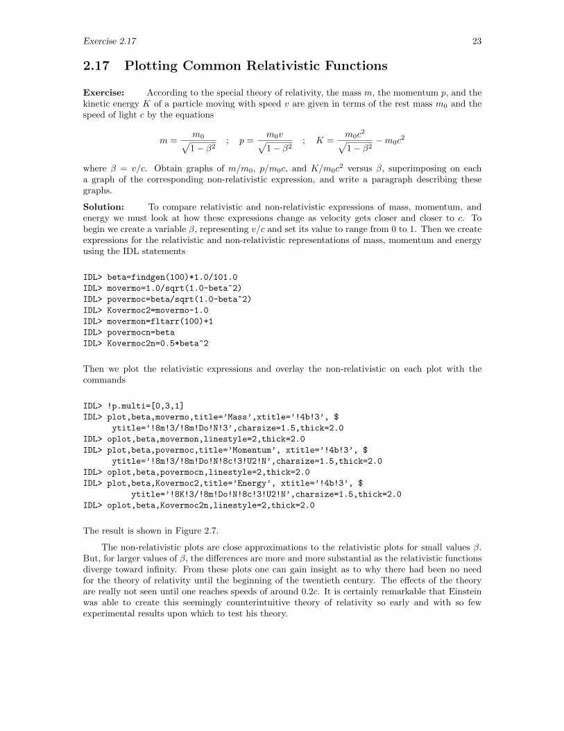
2.17 Plotting Common Relativistic Functions
Exercise: According to the special theory of relativity, the mass m, the momentum p, and thekinetic energy K of a particle moving with speed v are given in terms of the rest mass m0 and thespeed of light c by the equations
m =m0√1− β2
; p =m0v√1− β2
; K =m0c
2√1− β2
−m0c2
where β = v/c. Obtain graphs of m/m0, p/m0c, and K/m0c2 versus β, superimposing on each
a graph of the corresponding non-relativistic expression, and write a paragraph describing thesegraphs.
Solution: To compare relativistic and non-relativistic expressions of mass, momentum, andenergy we must look at how these expressions change as velocity gets closer and closer to c. Tobegin we create a variable β, representing v/c and set its value to range from 0 to 1. Then we createexpressions for the relativistic and non-relativistic representations of mass, momentum and energyusing the IDL statements
IDL> beta=findgen(100)*1.0/101.0
IDL> movermo=1.0/sqrt(1.0-beta^2)
IDL> povermoc=beta/sqrt(1.0-beta^2)
IDL> Kovermoc2=movermo-1.0
IDL> movermon=fltarr(100)+1
IDL> povermocn=beta
IDL> Kovermoc2n=0.5*beta^2
Then we plot the relativistic expressions and overlay the non-relativistic on each plot with thecommands
IDL> !p.multi=[0,3,1]
IDL> plot,beta,movermo,title=’Mass’,xtitle=’!4b!3’, $
ytitle=’!8m!3/!8m!Do!N!3’,charsize=1.5,thick=2.0
IDL> oplot,beta,movermon,linestyle=2,thick=2.0
IDL> plot,beta,povermoc,title=’Momentum’, xtitle=’!4b!3’, $
ytitle=’!8m!3/!8m!Do!N!8c!3!U2!N’,charsize=1.5,thick=2.0
IDL> oplot,beta,povermocn,linestyle=2,thick=2.0
IDL> plot,beta,Kovermoc2,title=’Energy’, xtitle=’!4b!3’, $
ytitle=’!8K!3/!8m!Do!N!8c!3!U2!N’,charsize=1.5,thick=2.0
IDL> oplot,beta,Kovermoc2n,linestyle=2,thick=2.0
The result is shown in Figure 2.7.
The non-relativistic plots are close approximations to the relativistic plots for small values β.But, for larger values of β, the differences are more and more substantial as the relativistic functionsdiverge toward infinity. From these plots one can gain insight as to why there had been no needfor the theory of relativity until the beginning of the twentieth century. The effects of the theoryare really not seen until one reaches speeds of around 0.2c. It is certainly remarkable that Einsteinwas able to create this seemingly counterintuitive theory of relativity so early and with so fewexperimental results upon which to test his theory.
24 Exercise 2.17
Figure 2.7: Relativistic versus non-relativistic dependence of mass ratio, momentum ratio, andenergy ratio on v/c. Relativistic functions are plotted using solid lines and non-relativistic functionsare plotted using dashed lines.
Exercise 2.18 25
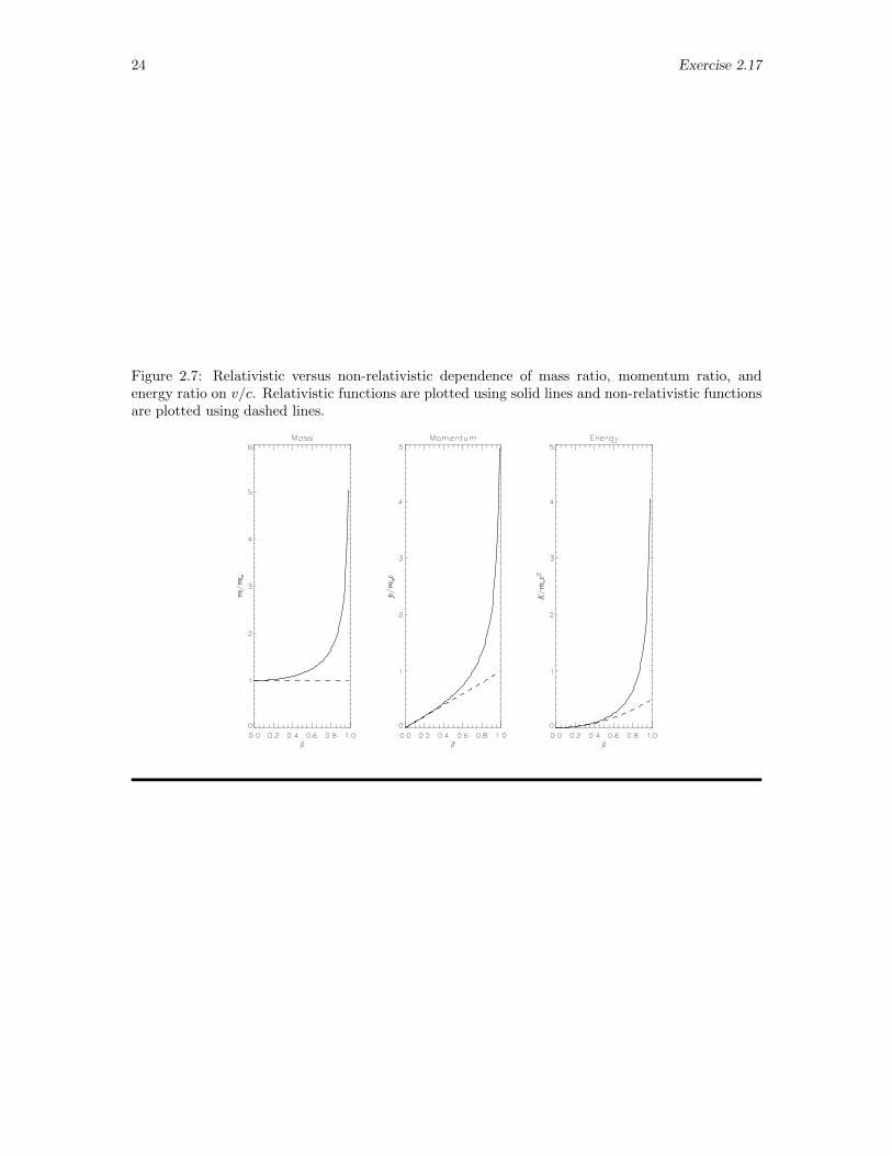
2.18 Plotting Transmission/Reflection of Thin Film
Exercise: In a vacuum, the transmission and reflection coefficients T and R of a dielectric filmof thickness d and index of refraction n are given by the equations
T =4n2
4n2 + (n2 − 1)2 sin2(κd); R =
(n2 − 1)2 sin2(κd)
4n2 + (n2 − 1)2 sin2(κd)(2.1)
where κ = 2πn/λ and λ is the wavelength of the wave in vacuum. Obtain graphs of T and R versusλ/d for various values of n and write a paragraph describing these graphs. Warning : Don’t tryplotting too close to λ = 0 since the function sin(κd) gives trouble at that point.
Solution: As stated in the exercise, the transmission and reflection coefficients of interest aregiven by
T =4n2
4n2 + (n2 − 1)2 sin2(κd); R =
(n2 − 1)2 sin2(κd)
4n2 + (n2 − 1)2 sin2(κd)
(Note, incidentally, that these expressions add to 1, as they must, since everything is either reflectedor transmitted.) We want, however, to plot these expressions as functions of wavelength λ, withwavelength measured in units of d. Thus, we recognize that
κd =2πd
λ=
2π
λwhere λ =
λ
d
In terms of λ, R and T are given by
T =4n2
4n2 + (n2 − 1)2 sin2(2π/λ); R =
(n2 − 1)2 sin2(2π/λ)
4n2 + (n2 − 1)2 sin2(2π/λ)
In plotting these quantities for various values of n as functions of λ, we must be wary of valuestoo close to λ = 0, since the sine functions oscillate increasingly rapidly as this limit is approached.Thus, we choose to plot over the interval 0.1 ≤ λ ≤ 6.0. Further, we note that we will need to usea large number of points to reproduce even reasonably accurate graphs for small values of λ. Weevaluate these functions for selected values of n with the statements
IDL> lambda = 6.0 * findgen(591)/600.0 + 0.1
IDL> n = 1.0
IDL> numT = 4.0*n^2 & numR = (n^2-1.0)^2*sin(2*!pi/lambda)^2
IDL> den = numT + numR
IDL> T1 = numT/den & R1 = numR/den
IDL> n = 1.5
IDL> numT = 4.0*n^2 & numR = (n^2-1.0)^2*sin(2*!pi/lambda)^2
IDL> den = numT + numR
IDL> T2 = numT/den & R2 = numR/den
IDL> n = 2.0
IDL> numT = 4.0*n^2 & numR = (n^2-1.0)^2*sin(2*!pi/lambda)^2
IDL> den = numT + numR
IDL> T3 = numT/den & R3 = numR/den
IDL> n = 3.0
IDL> numT = 4.0*n^2 & numR = (n^2-1.0)^2*sin(2*!pi/lambda)^2
IDL> den = numT + numR
IDL> T4 = numT/den & R4 = numR/den
Then, we plot R and T for these four values of n with the statements
26 Exercise 2.18
Figure 2.8: Transmission (upper curve in each frame at λ/d = 2) and reflection (lower curve in eachframe at λ/d = 2) coefficients T and R for the indicated values of the index of refraction n.
IDL> !p.multi=[0,2,2] & !y.range=[-0.5,1.5]
IDL> plot, lambda, T1, thick=3, xtitle=’!4k!3/d’, ytitle=’R, T’, title=’n=1.0’
IDL> oplot, lambda, R1, thick=3
IDL> plot, lambda, T2, thick=3, xtitle=’!4k!3/d’, ytitle=’R, T’, title=’n=1.5’
IDL> oplot, lambda, R2, thick=3
IDL> plot, lambda, T3, thick=3, xtitle=’!4k!3/d’, ytitle=’R, T’, title=’n=2.0’
IDL> oplot, lambda, R3, thick=3
IDL> plot, lambda, T4, thick=3, xtitle=’!4k!3/d’, ytitle=’R, T’, title=’n=3.0’
IDL> oplot, lambda, R4, thick=3
The resulting graph is shown in Fig. 2.8. Note that, when n = 1, there is basically no difference inthe two media involved so the incident beam is 100% transmitted and 0% reflected. As the index ofrefraction rises above 1, transmission and reflection begin to depend on wavelength, but always insuch a way that R+ T = 1.
Exercise 2.19 27
2.19 Plotting the Potential of Two Charged Disks
Exercise: Consider two circular disks, each of radius R, located with their centers on the z axissuch that their planes are parallel to the xy plane. Let the first disk have its center at the point(0, 0, b/2) and the second at the point (0, 0,−b/2) so that the disks are separated by a distance b(b > 0) and the origin is halfway between them. If the top disk carries a uniform, constant chargedensity σ and the bottom disk carries a uniform, constant charge density −σ, the electrostaticpotential at the point (0, 0, z) is given by
V (z) =σ
2ε0
√R2 +
(z − b
2
)2
−∣∣∣∣z − b
2
∣∣∣∣−√R2 +
(z +
b
2
)2
+
∣∣∣∣z +b
2
∣∣∣∣
Obtain graphs of V (z)/(σR/2ε0) versus z/R for various values of b/R and write a paragraph de-scribing these graphs. Hint : Remember the IDL function abs.
Solution: Starting with the expression above, we factor an R out of each term on the right tofind that
V (z)
σR/2ε0=
√1 +
(z
R− b
2R
)2
−∣∣∣∣ zR − b
2R
∣∣∣∣−√
1 +
(z
R+
b
2R
)2
+
∣∣∣∣ zR +b
2R
∣∣∣∣
Then, if we introduce the dimensionless variables z = z/R, b = b/R, and V = V (z)/(σR/2ε0), wecan write this expression still more compactly in the form
V =
√1 +
(z − b
2
)2
−∣∣∣∣z − b
2
∣∣∣∣−√
1 +
(z +
b
2
)2
+
∣∣∣∣z +b
2
∣∣∣∣
We then evaluate this expression as a function of z for various values of b with the statements
IDL> zbar = findgen(401)/50.0 - 4.0
IDL> bbar = 0.1
IDL> tmp1 = zbar - bbar/2.0 & tmp2 = zbar + bbar/2.0
IDL> V1 = sqrt(1+tmp1^2) - abs(tmp1) - sqrt(1+tmp2^2) + abs(tmp2)
IDL> bbar = 0.4
IDL> tmp1 = zbar - bbar/2.0 & tmp2 = zbar + bbar/2.0
IDL> V2 = sqrt(1+tmp1^2) - abs(tmp1) - sqrt(1+tmp2^2) + abs(tmp2)
IDL>
IDL> Repeat with bbar = 0.9, 1.6, 2.5, 3.6, generating V3, V4, V5, V6
IDL>
Finally, we plot graphs of these functions with the statements
IDL> !y.range = [-1.0,1.0] & !p.multi = [0,3,2]
IDL> plot, zbar, V1, thick=3.0, title=’b/R=0.1’
IDL> plot, zbar, V2, thick=3.0, title=’b/R=0.4’
IDL> plot, zbar, V3, thick=3.0, title=’b/R=0.9’
IDL> plot, zbar, V4, thick=3.0, title=’b/R=1.6’
IDL> plot, zbar, V5, thick=3.0, title=’b/R=2.5’
IDL> plot, zbar, V6, thick=3.0, title=’b/R=3.6’
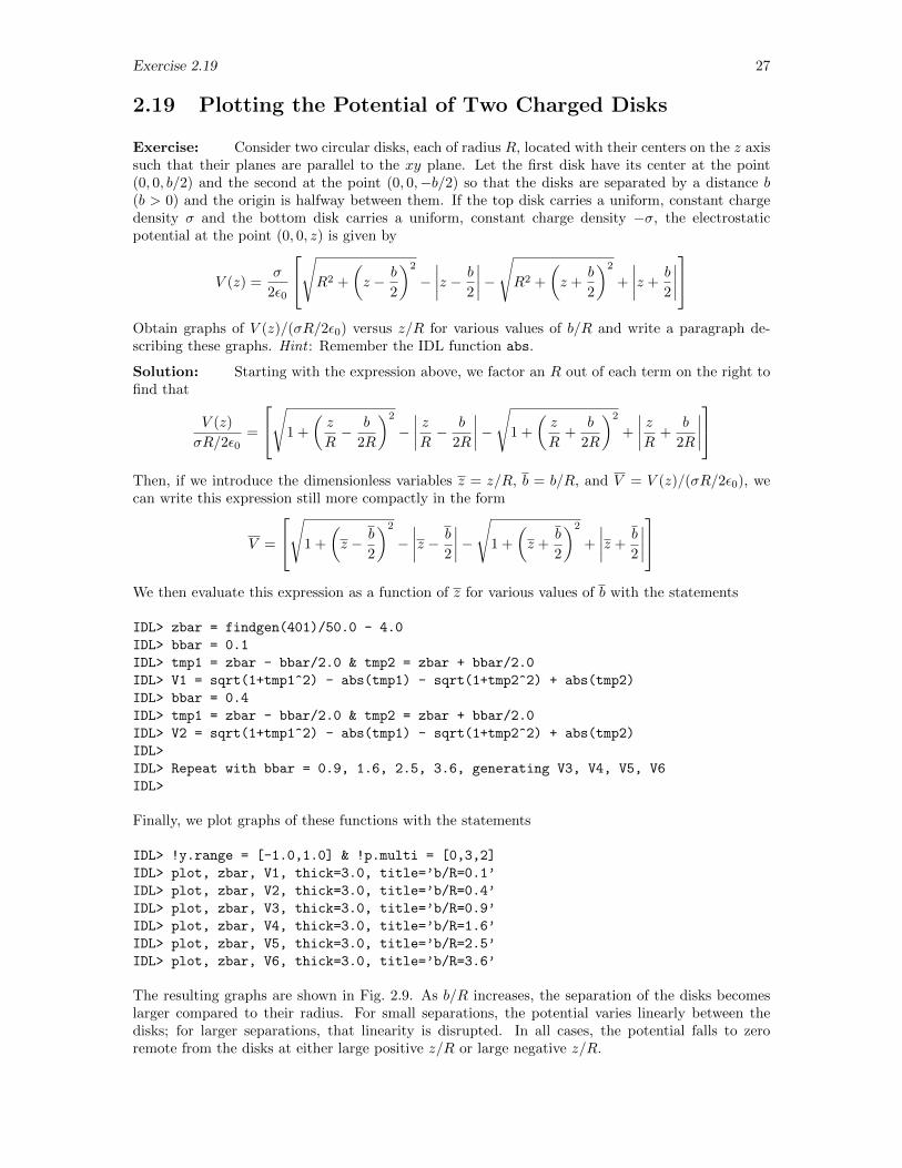
The resulting graphs are shown in Fig. 2.9. As b/R increases, the separation of the disks becomeslarger compared to their radius. For small separations, the potential varies linearly between thedisks; for larger separations, that linearity is disrupted. In all cases, the potential falls to zeroremote from the disks at either large positive z/R or large negative z/R.
28 Exercise 2.19
Figure 2.9: Graph of V (z)/(σR/2ε0) versus z/R for the indicated values of b/R.
Exercise 2.22 29
2.22 Plotting Relativistic Functions: Compton Effect
Exercise: When a photon of initial energy E0 undergoes Compton scattering from an atom ofmass m and is scattered by an angle θ, the energy of the photon is reduced to
E(θ) =E0
1 + ξ(1 + cos θ)
where ξ = E0/mc2. Obtain both Cartesian and polar graphs of E(θ)/E0 versus θ, −π ≤ θ ≤ π, for
several values of ξ, and write a paragraph describing these graphs.
Solution: To graph the function
E(θ)
E0=
1
1 + ξ(1 + cos θ)
over the interval −π ≤ θ ≤ π, we begin by establishing a vector with values of the independentvariable. For convenience in labeling the axes, we elect to generate an array both of values rangingfrom −1 to +1 and values ranging from −π to +π by invoking the statements2
x = findgen(101)/50.0 -1.0
theta = !pi*x
Then, we set a value for the parameter ξ, evaluate the function, and plot the values with thestatements
xi = 0.5
E = 1.0/(1.0+xi*(1.0+cos(theta)))
plot, x, E, thick=3.0
The resulting graph is combined with others in Fig. 2.10. With this graph alone, we are led to exploreother values of the parameter ξ and to construct a composite graph them all with the statements
plot, x, E, /nodata, xtitle = ’!4h!3 (rad)/!4p!3’, $
ytitle=’E(!4h!3)/E!D0!N’
xi = [ 0.1, 0.2, 0.3, 0.5, 0.75, 1.0, 2.0, 4.0 ]
for i = 0, 7 do begin $
E = 1.0/(1.0+xi[i]*(1.0+cos(theta))) & $
oplot, x, E, thick=3.0 & $
endfor
xyouts, -0.12, 0.87, ’!4n!3=0.1’
xyouts, -0.12, 0.06, ’!4n!3=4.0’
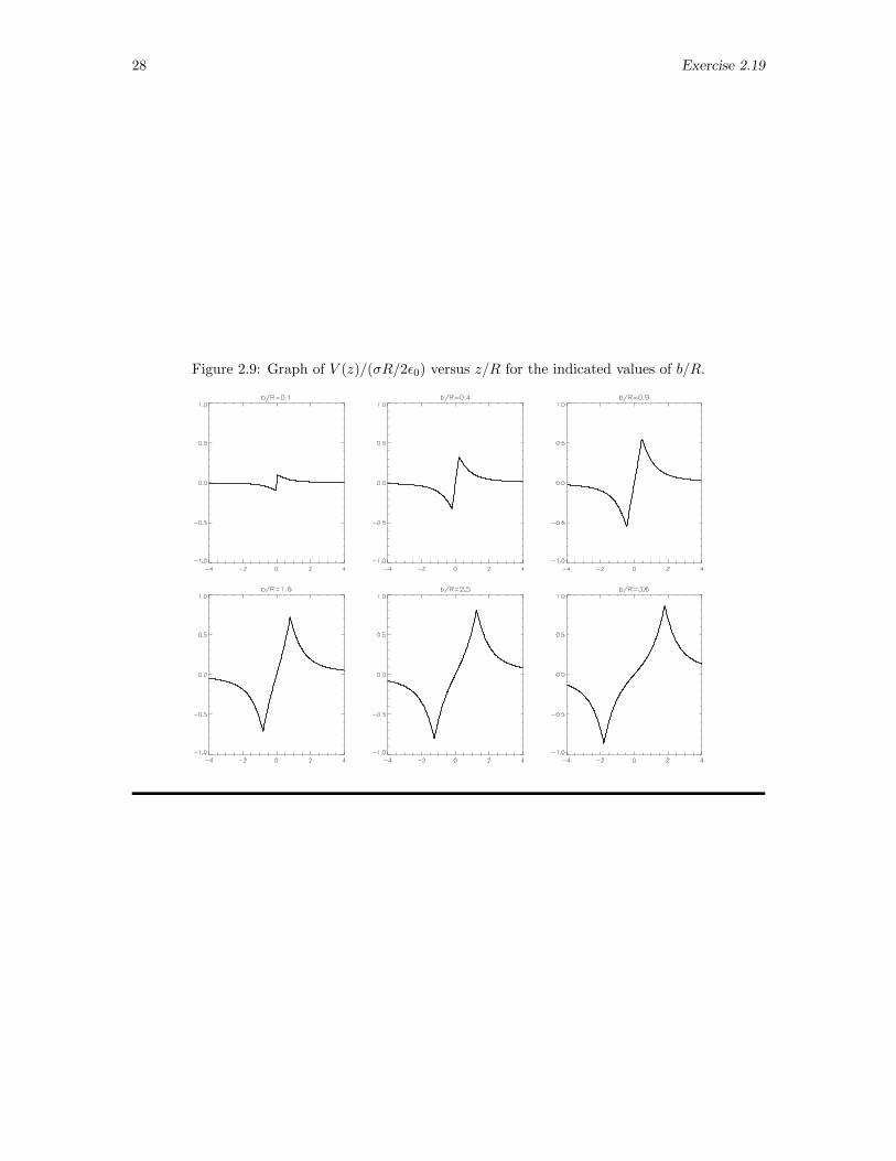
Whatever the ratio of photon energy to atomic rest energy, the photon energy is reduced by thelargest fraction for forward scattering (θ = 0) and is not reduced at all for backscattering (θ = +πor −π. Further, the greater the photon energy, the more greater its percentage loss of energy at anyscattering angle.
We can also create polar graphs of this function with the statements
E = 1.0/(1.0+xi[0]*(1.0+cos(theta)))
plot, E, theta, /polar, /nodata, xstyle=4, ystyle=4
for i = 0, 7 do begin $
2To facilitate cutting and pasting from the file accumulating this solution to the IDL command window, I elect toomit the IDL prompt from each line of code.
30 Exercise 2.22
Figure 2.10: E(θ)/E0 versus θ for various values of ξ = v/c.
E = 1.0/(1.0+xi[i]*(1.0+cos(theta))) & $
oplot, E, theta, /polar, thick=3.0 & $
endfor
oplot, [-1.0,1.0],[0.0,0.0]
oplot, [0.0,0.0], [-1.0,1.0]
xyouts, 1.0,0.05, ’0!Uo!N’
xyouts, 0.05,1.0, ’90!Uo!N’
xyouts, 0.65, 0.65, ’!4n!3=0.1’
xyouts, -0.5, 0.20, ’!4n!3=4.0’
This output is shown in Fig. 2.11. The conclusions we draw are the same as those drawn at the endof the previous paragraph.

Exercise 2.22 31
Figure 2.11: Polar plot of E(θ)/E0 versus θ for various values of ξ = v/c.
32 Exercise 2.23
2.23 Field of a Moving Charge
Exercise: A charged particle moves along the z-axis with speed v. When the particle passesthrough the origin, the magnitude of the electric field produced by the particle is given by theexpression
E(θ) =q
4πε0r2
1− β2
(1 + β2 sin2(θ))3/2
where θ is the polar angle of the observation point, r is the radial coordinate at that point, andβ = v/c. (c is the speed of light.) Obtain graphs of E(θ) = (q/4πε0r
2) versus θ and, to reveal someof the behavior more visibly, of E(θ)/E(0) versus θ for various values of β on the interval pi ≤ θ ≤ π,and write a paragraph describing these graphs.
Since we are asked to obtain (dimensionless) graphs of E/(q/4πε0r2) versus values of θ, and we
know that β < 1 always (since v ≤ c), we can simply write a sequence of IDL statements that willtake a bunch of β’s and output graphs of the E-fields using the code
dtheta = 2.0*!pi/100.0
theta = dtheta*findgen(101) - !pi
thetapl = 2.0/100.0 * findgen(101) - 1.0
beta = [ 0.2, 0.4, 0.6, 0.8, 0.99]
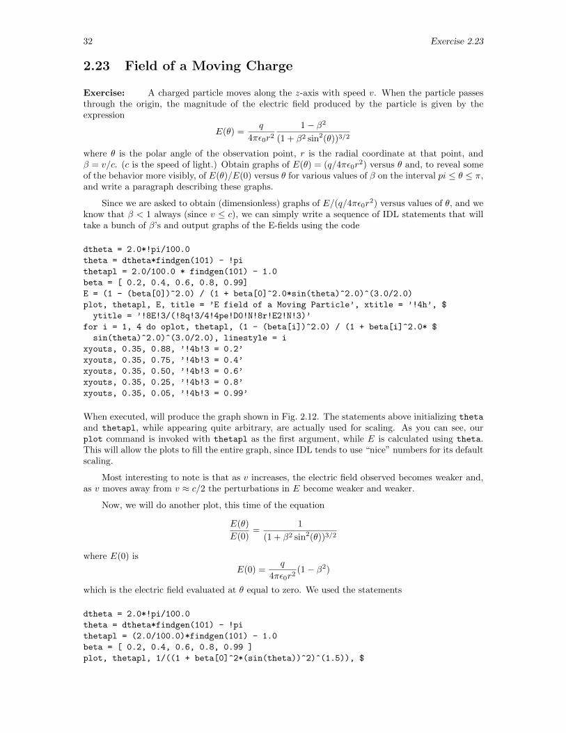
E = (1 - (beta[0])^2.0) / (1 + beta[0]^2.0*sin(theta)^2.0)^(3.0/2.0)
plot, thetapl, E, title = ’E field of a Moving Particle’, xtitle = ’!4h’, $
ytitle = ’!8E!3/(!8q!3/4!4pe!D0!N!8r!E2!N!3)’
for i = 1, 4 do oplot, thetapl, (1 - (beta[i])^2.0) / (1 + beta[i]^2.0* $
sin(theta)^2.0)^(3.0/2.0), linestyle = i
xyouts, 0.35, 0.88, ’!4b!3 = 0.2’
xyouts, 0.35, 0.75, ’!4b!3 = 0.4’
xyouts, 0.35, 0.50, ’!4b!3 = 0.6’
xyouts, 0.35, 0.25, ’!4b!3 = 0.8’
xyouts, 0.35, 0.05, ’!4b!3 = 0.99’
When executed, will produce the graph shown in Fig. 2.12. The statements above initializing theta
and thetapl, while appearing quite arbitrary, are actually used for scaling. As you can see, ourplot command is invoked with thetapl as the first argument, while E is calculated using theta.This will allow the plots to fill the entire graph, since IDL tends to use “nice” numbers for its defaultscaling.
Most interesting to note is that as v increases, the electric field observed becomes weaker and,as v moves away from v ≈ c/2 the perturbations in E become weaker and weaker.
Now, we will do another plot, this time of the equation
E(θ)
E(0)=
1
(1 + β2 sin2(θ))3/2
where E(0) is
E(0) =q
4πε0r2(1− β2)
which is the electric field evaluated at θ equal to zero. We used the statements
dtheta = 2.0*!pi/100.0
theta = dtheta*findgen(101) - !pi
thetapl = (2.0/100.0)*findgen(101) - 1.0
beta = [ 0.2, 0.4, 0.6, 0.8, 0.99 ]
plot, thetapl, 1/((1 + beta[0]^2*(sin(theta))^2)^(1.5)), $
Exercise 2.23 33
Figure 2.12: Various values of E/(q/4πε0r2) vs θ for different β
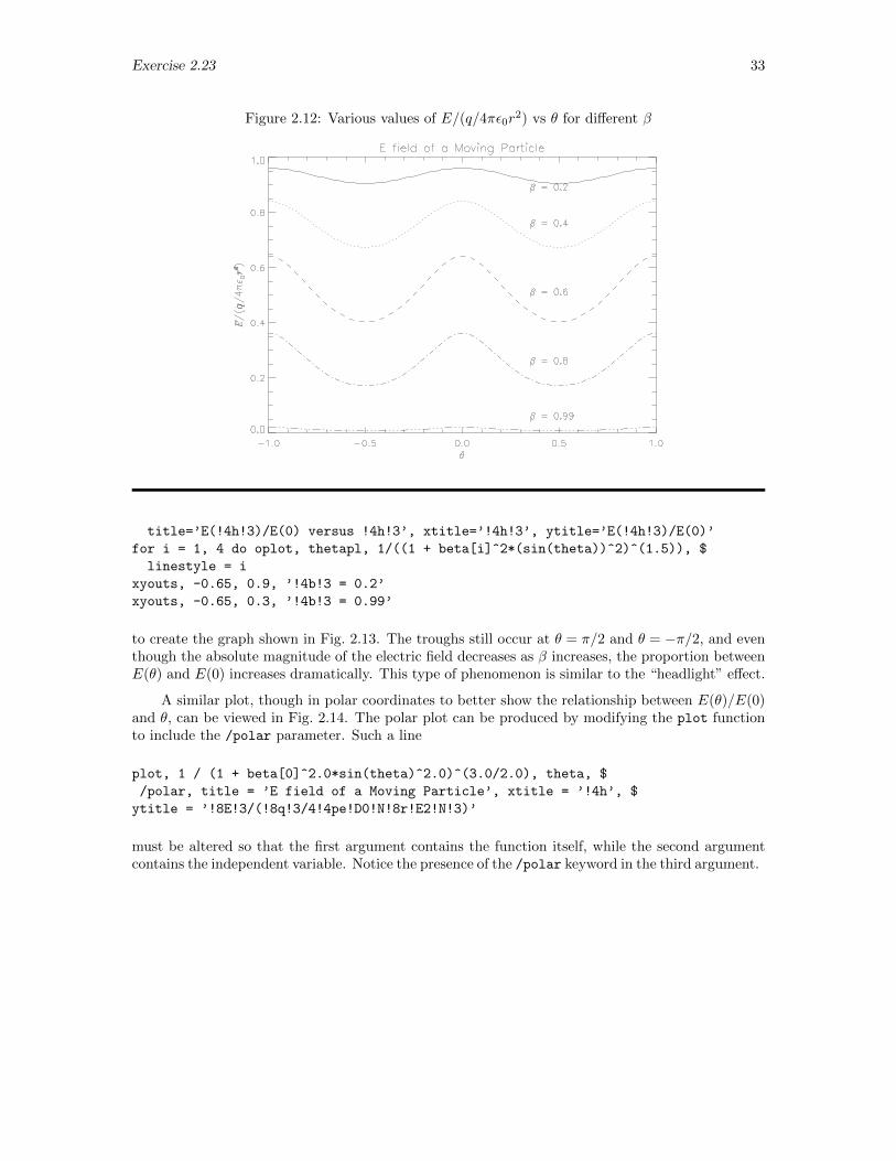
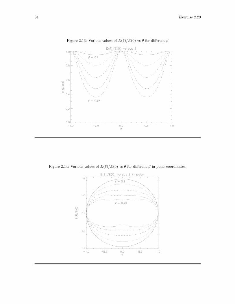
title=’E(!4h!3)/E(0) versus !4h!3’, xtitle=’!4h!3’, ytitle=’E(!4h!3)/E(0)’
for i = 1, 4 do oplot, thetapl, 1/((1 + beta[i]^2*(sin(theta))^2)^(1.5)), $
linestyle = i
xyouts, -0.65, 0.9, ’!4b!3 = 0.2’
xyouts, -0.65, 0.3, ’!4b!3 = 0.99’
to create the graph shown in Fig. 2.13. The troughs still occur at θ = π/2 and θ = −π/2, and eventhough the absolute magnitude of the electric field decreases as β increases, the proportion betweenE(θ) and E(0) increases dramatically. This type of phenomenon is similar to the “headlight” effect.
A similar plot, though in polar coordinates to better show the relationship between E(θ)/E(0)and θ, can be viewed in Fig. 2.14. The polar plot can be produced by modifying the plot functionto include the /polar parameter. Such a line
plot, 1 / (1 + beta[0]^2.0*sin(theta)^2.0)^(3.0/2.0), theta, $
/polar, title = ’E field of a Moving Particle’, xtitle = ’!4h’, $
ytitle = ’!8E!3/(!8q!3/4!4pe!D0!N!8r!E2!N!3)’
must be altered so that the first argument contains the function itself, while the second argumentcontains the independent variable. Notice the presence of the /polar keyword in the third argument.
34 Exercise 2.23
Figure 2.13: Various values of E(θ)/E(0) vs θ for different β
Figure 2.14: Various values of E(θ)/E(0) vs θ for different β in polar coordinates.
Exercise 2.24 35
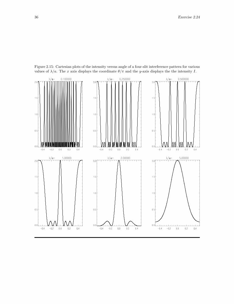
2.24 Plotting the Four-Slit Interference Pattern
Exercise: The intensity of the interference pattern produced by four slits illuminated by lightof wavelength λ when each slit is separated from the next by a distance a is given by
I(δ) = cos2 δ (1 + cos δ)
where δ = 2πa sin θ/λ. Obtain both Cartesian and polar graphs of I versus θ on the interval−π/2 ≤ θ ≤ π/2 for various values of λ/a, and write a paragraph describing these graphs.
Solution: When illuminated by a wave of wavelength λ, an array of four slits, each a distancea from its nearest neighbors, generates interesting interference patterns. To explore these patternscomputationally, we begin by forming a vector of values for θ ranging from −π/2 to π/2 and, so theplotting can be done on a horizontal scale labeled in multiples of π, an identically sized vector ofvalues ranging from −0.5 to +0.5. To that end, we invoke the statements
IDL> dt=1.0/1000.0
IDL> xaxis = -0.5+ dt*findgen(1001)
IDL> theta= !pi*xaxis
where, because we anticipate a function that varies rapidly in the interval −π/2 ≤ θ ≤ π/2, we putwhat might seem to be an unusually large number of points in the interval. Then, we form a vectorof values for λ/a that we want to look at. Here, we create an appropriate vector explicitly with thestatement
IDL> lambdaovera = [ 0.1, 0.25, 0.5, 1.0, 2.0, 5.0 ]
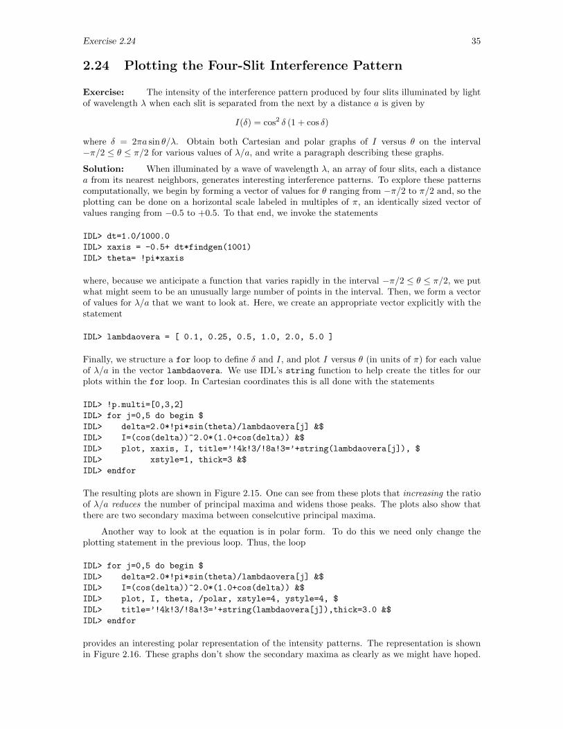
Finally, we structure a for loop to define δ and I, and plot I versus θ (in units of π) for each valueof λ/a in the vector lambdaovera. We use IDL’s string function to help create the titles for ourplots within the for loop. In Cartesian coordinates this is all done with the statements
IDL> !p.multi=[0,3,2]
IDL> for j=0,5 do begin $
IDL> delta=2.0*!pi*sin(theta)/lambdaovera[j] &$
IDL> I=(cos(delta))^2.0*(1.0+cos(delta)) &$
IDL> plot, xaxis, I, title=’!4k!3/!8a!3=’+string(lambdaovera[j]), $
IDL> xstyle=1, thick=3 &$
IDL> endfor
The resulting plots are shown in Figure 2.15. One can see from these plots that increasing the ratioof λ/a reduces the number of principal maxima and widens those peaks. The plots also show thatthere are two secondary maxima between conselcutive principal maxima.
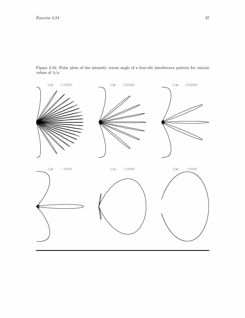
Another way to look at the equation is in polar form. To do this we need only change theplotting statement in the previous loop. Thus, the loop
IDL> for j=0,5 do begin $
IDL> delta=2.0*!pi*sin(theta)/lambdaovera[j] &$
IDL> I=(cos(delta))^2.0*(1.0+cos(delta)) &$
IDL> plot, I, theta, /polar, xstyle=4, ystyle=4, $
IDL> title=’!4k!3/!8a!3=’+string(lambdaovera[j]),thick=3.0 &$
IDL> endfor
provides an interesting polar representation of the intensity patterns. The representation is shownin Figure 2.16. These graphs don’t show the secondary maxima as clearly as we might have hoped.
36 Exercise 2.24
Figure 2.15: Cartesian plots of the intensity versus angle of a four-slit interference pattern for variousvalues of λ/a. The x axis displays the coordinate θ/π and the y-axis displays the the intensity I.
Exercise 2.24 37
Figure 2.16: Polar plots of the intensity versus angle of a four-slit interference pattern for variousvalues of λ/a.
38 Exercise 2.25
2.25 Plotting the Planck Blackbody Radiation Curve
Exercise: The Planck radiation law gives the expression
u(λ, T ) =8πch
λ5
1
ech/(λkT ) − 1
for the distribution of energy in the radiation emitted by a black body. Here, c is the speed of light,h is Planck’s constant, k is Boltzmann’s constant, λ is the wavelength of the radiation, and T is theabsolute temperature. Using appropriate dimensionless units, plot this function (a) as a functionof λ for several T and (b) as a surface over the λT -plane. Write a paragraph about the way thepeak changes in position, height, and width as T changes. Hint : Choose a reference wavelengthλ0 arbitrarily and recast the expression in terms of the dimensionless variable λ = λ/λ0. Then,note that T0 = ch/(λ0k) has the dimensions of temperature and re-express the temperature T interms of the dimensionless quantity T = T/T0. (You might find it informative to evaluate T0 forλ0 = 550 nm.) With these changes, the expression to be plotted can be recast in the form
u(λ, T ) =u(λ, T )
8πch/λ50
=1/λ
5
e1/(λT ) − 1
and the question now becomes one of plotting this quantity using the dimensionless variables λ andT .
Solution: This exercise is best begun by casting the expression
u(λ, T ) =8πch
λ5
1
ech/λkT − 1
in a dimensionless form. Rather than exploiting the dimensionless casting based on the arbitrarilyselected wavelength suggested in the statement of the exercise, we elect instead to choose an arbitraryreference temperature T0 and introduce the dimensionless temperature T = T/T0 so that T = T0T .Then, note that
ch
λkT=
ch
λkT0T
from which we infer that the quantity ch/kT0 might make a suitable unit for the measurement of λ.Checking the units of this quantity, we find
units ofch
λT0=
(m/s)× (J s)
(J/K)×K= m
(Here, J = Joule and K = Kelvin.) Thus, we choose a reference length λ0 = ch/kT0 and introducethe dimensionless wavelength λ so that λ = λ0λ. With this notation, we then have that
u(λ, T ) =8πch
λ50λ
5
1
e1/λT − 1
As the final step in this preparation, we then elect to plot
u =u
8πch/λ50
=1
λ5
1
e1/λT − 1
Note before we go on that, if the reference temperature is 1000 K, then the reference length is
λ0 =ch
kT0=
(3× 10⁸) m/s× (6.6× 10⁻³⁴) J s
(1.38× 10⁻²³) J/K× 103 K= 14.3× 10⁻⁶ m = 14300 nm
A quick scaling of this result reveals that for T0 = 2500 K (approximately the temperature of atungsten light filament), λ0 = 5720 nm and for T0 = 6000 K (approximately the temperature of thesurface of the sun), λ0 = 2380 nm.
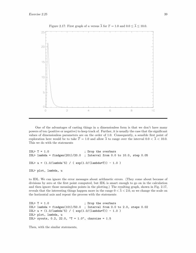
Exercise 2.25 39
Figure 2.17: First graph of u versus λ for T = 1.0 and 0.0 ≤ λ ≤ 10.0.
One of the advantages of casting things in a dimensionless form is that we don’t have manypowers of ten (positive or negative) to keep track of. Further, it is usually the case that the significantvalues of dimensionless parameters are on the order of 1.0. Consequently, a sensible first point ofexploration here would be to take T = 1.0 and allow λ to range over the interval 0.0 < λ < 10.0.This we do with the statements
IDL> T = 1.0 ; Drop the overbars
IDL> lambda = findgen(201)/20.0 ; Interval from 0.0 to 10.0, step 0.05
IDL> u = (1.0/lambda^5) / ( exp(1.0/(lambda*T)) - 1.0 )
IDL> plot, lambda, u
to IDL. We can ignore the error messages about arithmetic errors. (They come about because ofdivisions by zero at the first point computed, but IDL is smart enough to go on in the calculationand then ignore those meaningless points in the plotting.) The resulting graph, shown in Fig. 2.17,reveals that the interesting things happen more in the range 0 < λ < 2.0, so we change the scale onthe horizontal axis and repeat the process with the statements
IDL> T = 1.0 ; Drop the overbars
IDL> lambda = findgen(101)/50.0 ; Interval from 0.0 to 2.0, steps 0.02
IDL> u = (1.0/lambda^5) / ( exp(1.0/(lambda*T)) - 1.0 )
IDL> plot, lambda, u
IDL> xyouts, 0.2, 22.0, "T = 1.0", charsize = 1.5
Then, with the similar statements,
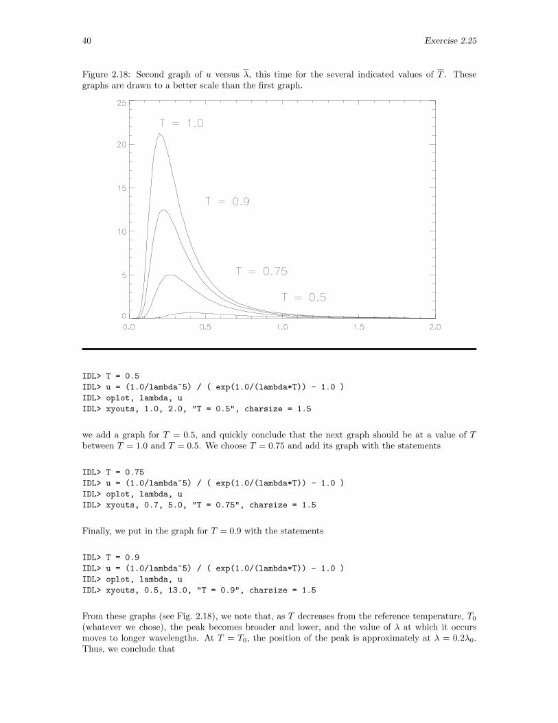
40 Exercise 2.25
Figure 2.18: Second graph of u versus λ, this time for the several indicated values of T . Thesegraphs are drawn to a better scale than the first graph.
IDL> T = 0.5
IDL> u = (1.0/lambda^5) / ( exp(1.0/(lambda*T)) - 1.0 )
IDL> oplot, lambda, u
IDL> xyouts, 1.0, 2.0, "T = 0.5", charsize = 1.5
we add a graph for T = 0.5, and quickly conclude that the next graph should be at a value of Tbetween T = 1.0 and T = 0.5. We choose T = 0.75 and add its graph with the statements
IDL> T = 0.75
IDL> u = (1.0/lambda^5) / ( exp(1.0/(lambda*T)) - 1.0 )
IDL> oplot, lambda, u
IDL> xyouts, 0.7, 5.0, "T = 0.75", charsize = 1.5
Finally, we put in the graph for T = 0.9 with the statements
IDL> T = 0.9
IDL> u = (1.0/lambda^5) / ( exp(1.0/(lambda*T)) - 1.0 )
IDL> oplot, lambda, u
IDL> xyouts, 0.5, 13.0, "T = 0.9", charsize = 1.5
From these graphs (see Fig. 2.18), we note that, as T decreases from the reference temperature, T0
(whatever we chose), the peak becomes broader and lower, and the value of λ at which it occursmoves to longer wavelengths. At T = T0, the position of the peak is approximately at λ = 0.2λ0.Thus, we conclude that
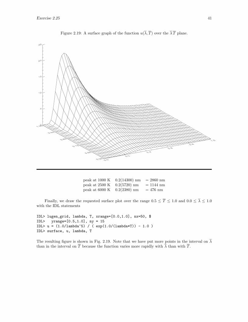
Exercise 2.25 41
Figure 2.19: A surface graph of the function u(λ, T ) over the λT plane.
peak at 1000 K 0.2(14300) nm = 2860 nmpeak at 2500 K 0.2(5720) nm = 1144 nmpeak at 6000 K 0.2(2380) nm = 476 nm
Finally, we draw the requested surface plot over the range 0.5 ≤ T ≤ 1.0 and 0.0 ≤ λ ≤ 1.0with the IDL statements
IDL> lugen_grid, lambda, T, xrange=[0.0,1.0], nx=50, $
IDL> yrange=[0.5,1.0], ny = 15
IDL> u = (1.0/lambda^5) / ( exp(1.0/(lambda*T)) - 1.0 )
IDL> surface, u, lambda, T
The resulting figure is shown in Fig. 2.19. Note that we have put more points in the interval on λthan in the interval on T because the function varies more rapidly with λ than with T .
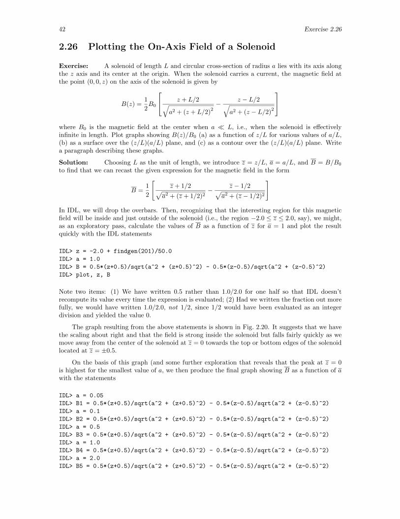
42 Exercise 2.26
2.26 Plotting the On-Axis Field of a Solenoid
Exercise: A solenoid of length L and circular cross-section of radius a lies with its axis alongthe z axis and its center at the origin. When the solenoid carries a current, the magnetic field atthe point (0, 0, z) on the axis of the solenoid is given by
B(z) =1
2B0
z + L/2√a2 + (z + L/2)
2− z − L/2√
a2 + (z − L/2)2
where B0 is the magnetic field at the center when a L, i.e., when the solenoid is effectivelyinfinite in length. Plot graphs showing B(z)/B0 (a) as a function of z/L for various values of a/L,(b) as a surface over the (z/L)(a/L) plane, and (c) as a contour over the (z/L)(a/L) plane. Writea paragraph describing these graphs.
Solution: Choosing L as the unit of length, we introduce z = z/L, a = a/L, and B = B/B0
to find that we can recast the given expression for the magnetic field in the form
B =1
2
[z + 1/2√
a2 + (z + 1/2)2− z − 1/2√
a2 + (z − 1/2)2
]
In IDL, we will drop the overbars. Then, recognizing that the interesting region for this magneticfield will be inside and just outside of the solenoid (i.e., the region −2.0 ≤ z ≤ 2.0, say), we might,as an exploratory pass, calculate the values of B as a function of z for a = 1 and plot the resultquickly with the IDL statements
IDL> z = -2.0 + findgen(201)/50.0
IDL> a = 1.0
IDL> B = 0.5*(z+0.5)/sqrt(a^2 + (z+0.5)^2) - 0.5*(z-0.5)/sqrt(a^2 + (z-0.5)^2)
IDL> plot, z, B
Note two items: (1) We have written 0.5 rather than 1.0/2.0 for one half so that IDL doesn’trecompute its value every time the expression is evaluated; (2) Had we written the fraction out morefully, we would have written 1.0/2.0, not 1/2, since 1/2 would have been evaluated as an integerdivision and yielded the value 0.
The graph resulting from the above statements is shown in Fig. 2.20. It suggests that we havethe scaling about right and that the field is strong inside the solenoid but falls fairly quickly as wemove away from the center of the solenoid at z = 0 towards the top or bottom edges of the solenoidlocated at z = ±0.5.
On the basis of this graph (and some further exploration that reveals that the peak at z = 0is highest for the smallest value of a, we then produce the final graph showing B as a function of awith the statements
IDL> a = 0.05
IDL> B1 = 0.5*(z+0.5)/sqrt(a^2 + (z+0.5)^2) - 0.5*(z-0.5)/sqrt(a^2 + (z-0.5)^2)
IDL> a = 0.1
IDL> B2 = 0.5*(z+0.5)/sqrt(a^2 + (z+0.5)^2) - 0.5*(z-0.5)/sqrt(a^2 + (z-0.5)^2)
IDL> a = 0.5
IDL> B3 = 0.5*(z+0.5)/sqrt(a^2 + (z+0.5)^2) - 0.5*(z-0.5)/sqrt(a^2 + (z-0.5)^2)
IDL> a = 1.0
IDL> B4 = 0.5*(z+0.5)/sqrt(a^2 + (z+0.5)^2) - 0.5*(z-0.5)/sqrt(a^2 + (z-0.5)^2)
IDL> a = 2.0
IDL> B5 = 0.5*(z+0.5)/sqrt(a^2 + (z+0.5)^2) - 0.5*(z-0.5)/sqrt(a^2 + (z-0.5)^2)
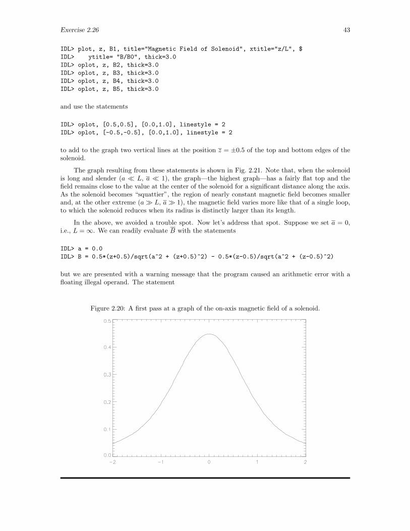
Exercise 2.26 43
IDL> plot, z, B1, title="Magnetic Field of Solenoid", xtitle="z/L", $
IDL> ytitle= "B/B0", thick=3.0
IDL> oplot, z, B2, thick=3.0
IDL> oplot, z, B3, thick=3.0
IDL> oplot, z, B4, thick=3.0
IDL> oplot, z, B5, thick=3.0
and use the statements
IDL> oplot, [0.5,0.5], [0.0,1.0], linestyle = 2
IDL> oplot, [-0.5,-0.5], [0.0,1.0], linestyle = 2
to add to the graph two vertical lines at the position z = ±0.5 of the top and bottom edges of thesolenoid.
The graph resulting from these statements is shown in Fig. 2.21. Note that, when the solenoidis long and slender (a L, a 1), the graph—the highest graph—has a fairly flat top and thefield remains close to the value at the center of the solenoid for a significant distance along the axis.As the solenoid becomes “squattier”, the region of nearly constant magnetic field becomes smallerand, at the other extreme (a L, a 1), the magnetic field varies more like that of a single loop,to which the solenoid reduces when its radius is distinctly larger than its length.
In the above, we avoided a trouble spot. Now let’s address that spot. Suppose we set a = 0,i.e., L =∞. We can readily evaluate B with the statements
IDL> a = 0.0
IDL> B = 0.5*(z+0.5)/sqrt(a^2 + (z+0.5)^2) - 0.5*(z-0.5)/sqrt(a^2 + (z-0.5)^2)
but we are presented with a warning message that the program caused an arithmetic error with afloating illegal operand. The statement
Figure 2.20: A first pass at a graph of the on-axis magnetic field of a solenoid.
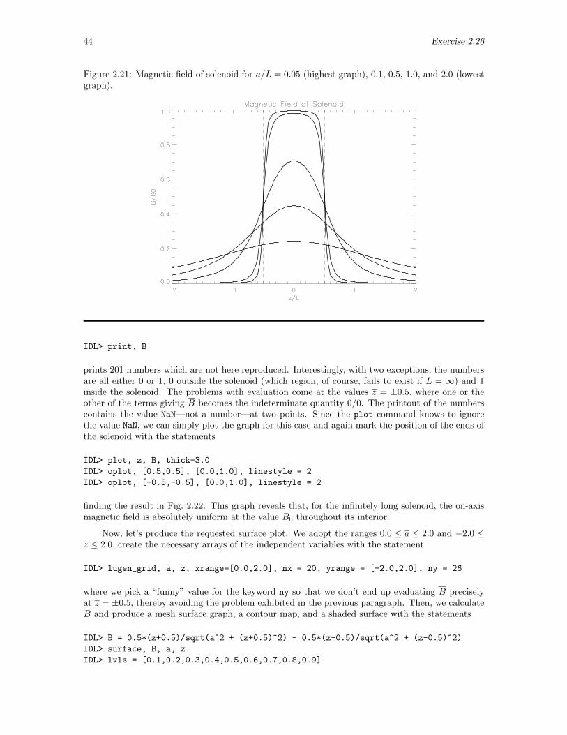
44 Exercise 2.26
Figure 2.21: Magnetic field of solenoid for a/L = 0.05 (highest graph), 0.1, 0.5, 1.0, and 2.0 (lowestgraph).
IDL> print, B
prints 201 numbers which are not here reproduced. Interestingly, with two exceptions, the numbersare all either 0 or 1, 0 outside the solenoid (which region, of course, fails to exist if L = ∞) and 1inside the solenoid. The problems with evaluation come at the values z = ±0.5, where one or theother of the terms giving B becomes the indeterminate quantity 0/0. The printout of the numberscontains the value NaN—not a number—at two points. Since the plot command knows to ignorethe value NaN, we can simply plot the graph for this case and again mark the position of the ends ofthe solenoid with the statements
IDL> plot, z, B, thick=3.0
IDL> oplot, [0.5,0.5], [0.0,1.0], linestyle = 2
IDL> oplot, [-0.5,-0.5], [0.0,1.0], linestyle = 2
finding the result in Fig. 2.22. This graph reveals that, for the infinitely long solenoid, the on-axismagnetic field is absolutely uniform at the value B0 throughout its interior.
Now, let’s produce the requested surface plot. We adopt the ranges 0.0 ≤ a ≤ 2.0 and −2.0 ≤z ≤ 2.0, create the necessary arrays of the independent variables with the statement
IDL> lugen_grid, a, z, xrange=[0.0,2.0], nx = 20, yrange = [-2.0,2.0], ny = 26
where we pick a “funny” value for the keyword ny so that we don’t end up evaluating B preciselyat z = ±0.5, thereby avoiding the problem exhibited in the previous paragraph. Then, we calculateB and produce a mesh surface graph, a contour map, and a shaded surface with the statements
IDL> B = 0.5*(z+0.5)/sqrt(a^2 + (z+0.5)^2) - 0.5*(z-0.5)/sqrt(a^2 + (z-0.5)^2)
IDL> surface, B, a, z
IDL> lvls = [0.1,0.2,0.3,0.4,0.5,0.6,0.7,0.8,0.9]
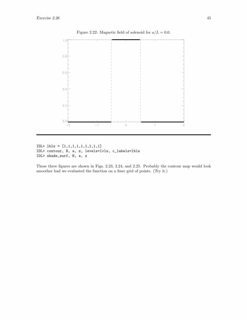
Exercise 2.26 45
Figure 2.22: Magnetic field of solenoid for a/L = 0.0.
IDL> lbls = [1,1,1,1,1,1,1,1,1]
IDL> contour, B, a, z, levels=lvls, c_labels=lbls
IDL> shade_surf, B, a, z
These three figures are shown in Figs. 2.23, 2.24, and 2.25. Probably the contour map would looksmoother had we evaluated the function on a finer grid of points. (Try it.)
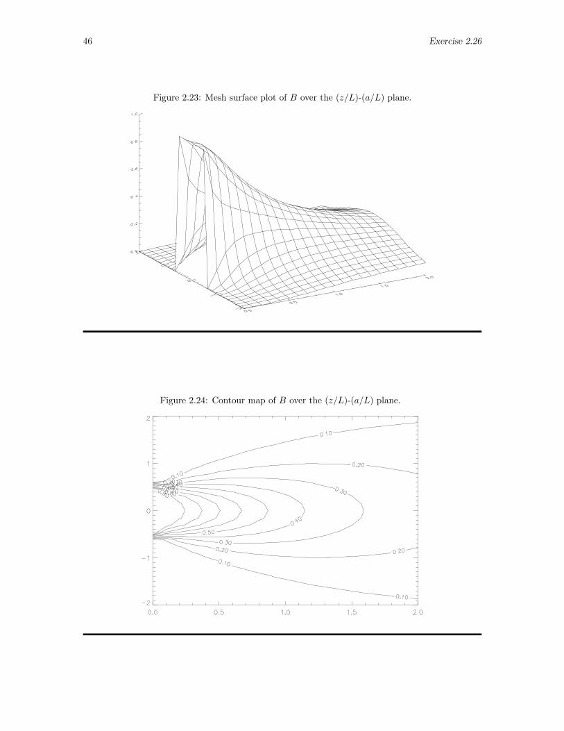
46 Exercise 2.26
Figure 2.23: Mesh surface plot of B over the (z/L)-(a/L) plane.
Figure 2.24: Contour map of B over the (z/L)-(a/L) plane.
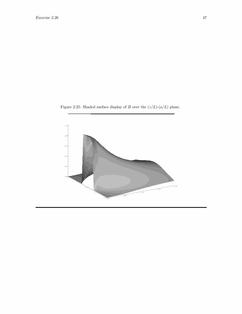
Exercise 2.26 47
Figure 2.25: Shaded surface display of B over the (z/L)-(a/L) plane.
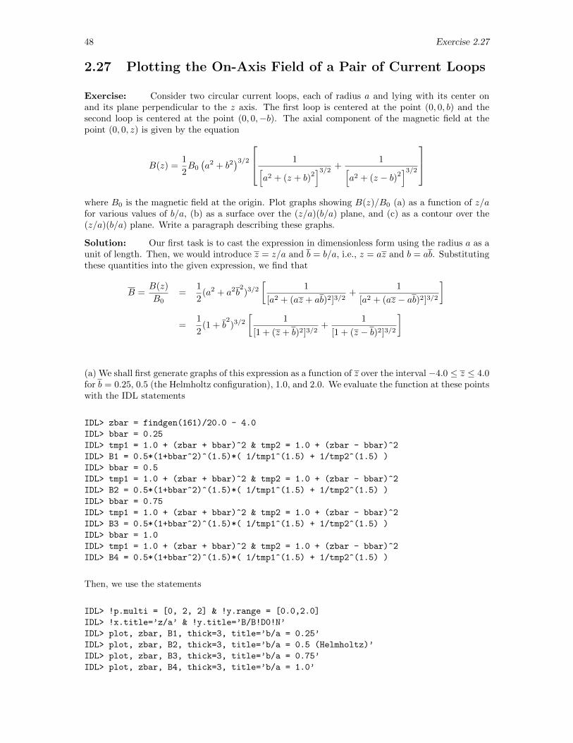
48 Exercise 2.27
2.27 Plotting the On-Axis Field of a Pair of Current Loops
Exercise: Consider two circular current loops, each of radius a and lying with its center onand its plane perpendicular to the z axis. The first loop is centered at the point (0, 0, b) and thesecond loop is centered at the point (0, 0,−b). The axial component of the magnetic field at thepoint (0, 0, z) is given by the equation
B(z) =1
2B0
(a2 + b2
)3/2 1[a2 + (z + b)
2]3/2 +
1[a2 + (z − b)2
]3/2
where B0 is the magnetic field at the origin. Plot graphs showing B(z)/B0 (a) as a function of z/afor various values of b/a, (b) as a surface over the (z/a)(b/a) plane, and (c) as a contour over the(z/a)(b/a) plane. Write a paragraph describing these graphs.
Solution: Our first task is to cast the expression in dimensionless form using the radius a as aunit of length. Then, we would introduce z = z/a and b = b/a, i.e., z = az and b = ab. Substitutingthese quantities into the given expression, we find that
B =B(z)
B0=
1
2(a2 + a2b
2)3/2
[1
[a2 + (az + ab)2]3/2+
1
[a2 + (az − ab)2]3/2
]
=1
2(1 + b
2)3/2
[1
[1 + (z + b)2]3/2+
1
[1 + (z − b)2]3/2
]
(a) We shall first generate graphs of this expression as a function of z over the interval −4.0 ≤ z ≤ 4.0for b = 0.25, 0.5 (the Helmholtz configuration), 1.0, and 2.0. We evaluate the function at these pointswith the IDL statements
IDL> zbar = findgen(161)/20.0 - 4.0
IDL> bbar = 0.25
IDL> tmp1 = 1.0 + (zbar + bbar)^2 & tmp2 = 1.0 + (zbar - bbar)^2
IDL> B1 = 0.5*(1+bbar^2)^(1.5)*( 1/tmp1^(1.5) + 1/tmp2^(1.5) )
IDL> bbar = 0.5
IDL> tmp1 = 1.0 + (zbar + bbar)^2 & tmp2 = 1.0 + (zbar - bbar)^2
IDL> B2 = 0.5*(1+bbar^2)^(1.5)*( 1/tmp1^(1.5) + 1/tmp2^(1.5) )
IDL> bbar = 0.75
IDL> tmp1 = 1.0 + (zbar + bbar)^2 & tmp2 = 1.0 + (zbar - bbar)^2
IDL> B3 = 0.5*(1+bbar^2)^(1.5)*( 1/tmp1^(1.5) + 1/tmp2^(1.5) )
IDL> bbar = 1.0
IDL> tmp1 = 1.0 + (zbar + bbar)^2 & tmp2 = 1.0 + (zbar - bbar)^2
IDL> B4 = 0.5*(1+bbar^2)^(1.5)*( 1/tmp1^(1.5) + 1/tmp2^(1.5) )
Then, we use the statements
IDL> !p.multi = [0, 2, 2] & !y.range = [0.0,2.0]
IDL> !x.title=’z/a’ & !y.title=’B/B!D0!N’
IDL> plot, zbar, B1, thick=3, title=’b/a = 0.25’
IDL> plot, zbar, B2, thick=3, title=’b/a = 0.5 (Helmholtz)’
IDL> plot, zbar, B3, thick=3, title=’b/a = 0.75’
IDL> plot, zbar, B4, thick=3, title=’b/a = 1.0’
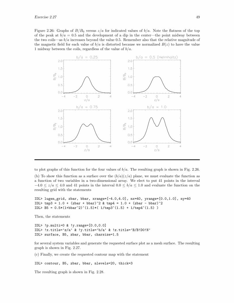
Exercise 2.27 49
Figure 2.26: Graphs of B/B0 versus z/a for indicated values of b/a. Note the flatness of the topof the peak at b/a = 0.5 and the development of a dip in the center—the point midway betweenthe two coils—as b/a increases beyond the value 0.5. Remember also that the relative magnitude ofthe magnetic field for each value of b/a is distorted because we normalized B(z) to have the value1 midway between the coils, regardless of the value of b/a.
to plot graphs of this function for the four values of b/a. The resulting graph is shown in Fig. 2.26.
(b) To show this function as a surface over the (b/a)(z/a) plane, we must evaluate the function asa function of two variables in a two-dimensional array. We elect to put 41 points in the interval−4.0 ≤ z/a ≤ 4.0 and 41 points in the interval 0.0 ≤ b/a ≤ 1.0 and evaluate the function on theresulting grid with the statements
IDL> lugen_grid, zbar, bbar, xrange=[-4.0,4.0], nx=40, yrange=[0.0,1.0], ny=40
IDL> tmp3 = 1.0 + (zbar + bbar)^2 & tmp4 = 1.0 + (zbar - bbar)^2
IDL> B5 = 0.5*(1+bbar^2)^(1.5)*( 1/tmp3^(1.5) + 1/tmp4^(1.5) )
Then, the statements
IDL> !p.multi=0 & !y.range=[0.0,0.0]
IDL> !x.title=’z/a’ & !y.title=’b/a’ & !z.title=’B/B!D0!N’
IDL> surface, B5, zbar, bbar, charsize=1.5
for several system variables and generate the requested surface plot as a mesh surface. The resultinggraph is shown in Fig. 2.27.
(c) Finally, we create the requested contour map with the statement
IDL> contour, B5, zbar, bbar, nlevels=20, thick=3
The resulting graph is shown in Fig. 2.28.
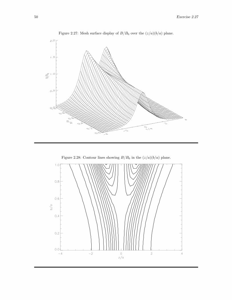
50 Exercise 2.27
Figure 2.27: Mesh surface display of B/B0 over the (z/a)(b/a) plane.
Figure 2.28: Contour lines showing B/B0 in the (z/a)(b/a) plane.
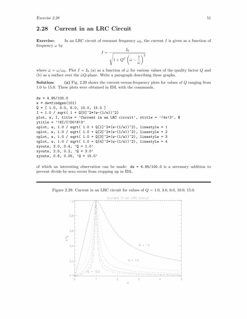
Exercise 2.28 51
2.28 Current in an LRC Circuit
Exercise: In an LRC circuit of resonant frequency ω0, the current I is given as a function offrequency ω by
I =I0√
1 +Q2
(ω − 1
ω
)2
where ω = ω/ω0. Plot I = I0 (a) as a function of ω for various values of the quality factor Q and(b) as a surface over the ωQ-plane. Write a paragraph describing these graphs.
Solution: (a) Fig. 2.29 shows the current-versus-frequency plots for values of Q ranging from1.0 to 15.0. These plots were obtained in IDL with the commands,
dw = 4.95/100.0
w = dw*findgen(101)
Q = [ 1.0, 3.0, 6.0, 10.0, 15.0 ]
I = 1.0 / sqrt( 1 + Q[0]^2*(w-(1/w))^2)
plot, w, I, title = ’Current in an LRC circuit’, xtitle = ’!4x!3’, $
ytitle = ’!8I/I!D0!N!3’
oplot, w, 1.0 / sqrt( 1.0 + Q[1]^2*(w-(1/w))^2), linestyle = 1
oplot, w, 1.0 / sqrt( 1.0 + Q[2]^2*(w-(1/w))^2), linestyle = 2
oplot, w, 1.0 / sqrt( 1.0 + Q[3]^2*(w-(1/w))^2), linestyle = 3
oplot, w, 1.0 / sqrt( 1.0 + Q[4]^2*(w-(1/w))^2), linestyle = 4
xyouts, 3.0, 0.4, ’Q = 1.0’
xyouts, 2.5, 0.2, ’Q = 3.0’
xyouts, 0.6, 0.05, ’Q = 15.0’
of which an interesting observation can be made: dw = 4.95/100.0 is a necessary addition toprevent divide-by-zero errors from cropping up in IDL.
Figure 2.29: Current in an LRC circuit for values of Q = 1.0, 3.0, 6.0, 10.0, 15.0.
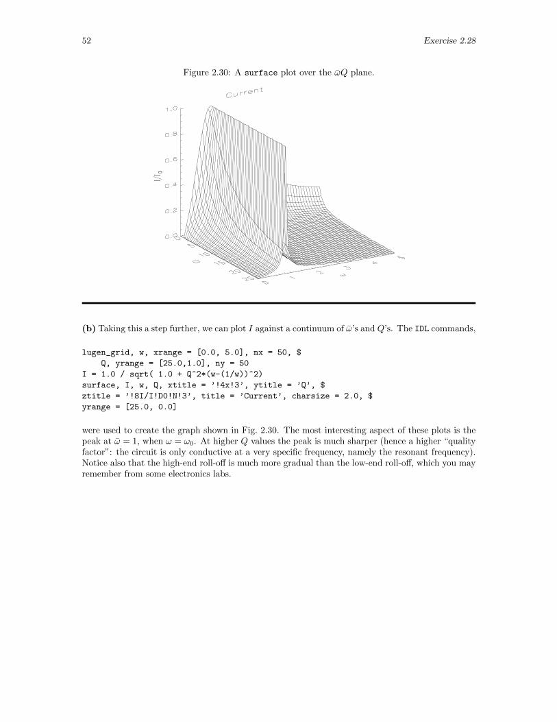
52 Exercise 2.28
Figure 2.30: A surface plot over the ωQ plane.
(b) Taking this a step further, we can plot I against a continuum of ω’s and Q’s. The IDL commands,
lugen_grid, w, xrange = [0.0, 5.0], nx = 50, $
Q, yrange = [25.0,1.0], ny = 50
I = 1.0 / sqrt( 1.0 + Q^2*(w-(1/w))^2)
surface, I, w, Q, xtitle = ’!4x!3’, ytitle = ’Q’, $
ztitle = ’!8I/I!D0!N!3’, title = ’Current’, charsize = 2.0, $
yrange = [25.0, 0.0]
were used to create the graph shown in Fig. 2.30. The most interesting aspect of these plots is thepeak at ω = 1, when ω = ω0. At higher Q values the peak is much sharper (hence a higher “qualityfactor”: the circuit is only conductive at a very specific frequency, namely the resonant frequency).Notice also that the high-end roll-off is much more gradual than the low-end roll-off, which you mayremember from some electronics labs.
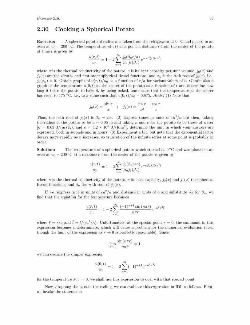
Exercise 2.30 53
2.30 Cooking a Spherical Potato
Exercise: A spherical potato of radius a is taken from the refrigerator at 0 C and placed in anoven at u0 = 200 C. The temperature u(r, t) at a point a distance r from the center of the potatoat time t is given by
u(r, t)
u0= 1− 2
∞∑n=1
j0(βnr/a)
βn j1(βn)e−κβ
2nt/(ca
2)
where κ is the thermal conductivity of the potato, c is its heat capacity per unit volume, j0(x) andj1(x) are the zeroth- and first-order spherical Bessel functions, and βn is the n-th root of j0(x), i.e.,j0(βn) = 0. Obtain graphs of u(r, t)/u0 as a function of r/a for various values of t. Obtain also agraph of the temperature u(0, t) at the center of the potato as a function of t and determine howlong it takes the potato to bake if, by being baked, one means that the temperature at the centerhas risen to 175 C, i.e., to a value such that u(0, t)/u0 = 0.875. Hints: (1) Note that
j0(x) =sinx
x; j1(x) =
sinx
x2− cosx
x
Thus, the n-th root of j0(x) is βn = nπ. (2) Express times in units of ca2/κ but then, takingthe radius of the potato to be a = 0.05 m and taking κ and c for the potato to be those of water[κ = 0.63 J/(m s K), and c = 4.2 × 10⁶ J/(K m3], determine the unit in which your answers areexpressed, both in seconds and in hours. (3) Experiment a bit, but note that the exponential factordecays more rapidly as n increases, so truncation of the infinite series at some point is probably inorder.
Solution: The temperature of a spherical potato which started at 0 C and was placed in anoven at u0 = 200 C at a distance r from the center of the potato is given by
u(r, t)
u0= 1− 2
∞∑n=1
j0(βnr/a)
βnj1(βn)e−κβ
2nt/(ca
2)
where κ is the thermal conductivity of the potato, c its heat capacity, j0(x) and j1(x) the sphericalBessel functions, and βn the n-th root of j0(x).
If we rexpress time in units of ca2/κ and distance in units of a and substitute nπ for βn, wefind that the equation for the temperature becomes
u(r, t)
u0= 1− 2
∞∑n=1
(−1)n+1 sin (nπr)
nπre−n
2π2 t
where r = r/a and t = t/(ca2/κ). Unfortunately, at the special point r = 0, the summand in thisexpression becomes indeterminate, which will cause a problem for the numerical evaluation (eventhough the limit of the expression as r → 0 is perfectly reasonable). Since
limr→0
sin(nπr)
nπr= 1
we can deduce the simpler expression
u(0, t)
u0= 1− 2
∞∑n=1
(−1)n+1e−n2π2 t
for the temperature at r = 0; we shall use this expression to deal with that special point.
Now, dropping the bars in the coding, we can evaluate this expression in IDL as follows. First,we invoke the statements
54 Exercise 2.30
IDL> dr = 1.0/100.0
IDL> r = dr*findgen(100) + dr
IDL> rplot = [ 0.0, r ]
to create values of r that avoid the point r = 0 and define the vector including the zero value forplotting purposes. Then, we choose a value of t and define the array u—including the first term (the1) in the expression—to receive temperatures as we find them by executing the statements
IDL> t = 0.01
IDL> u = fltarr(100) + 1.0
Then, for each of 100 values of r (index i, we sum (index n) over however many values of n wechoose to include in the sum. If we truncate the sum with n = 20, we would then evaluate u(r), addthe temperature at r = 0, and save the results in a unique variable with the statements
IDL> for i = 0, 99 do begin $
IDL> for n = 1, 20 do begin $
IDL> tmp = (-1)^(n+1)*sin(n*!pi*r[i])*exp(-n^2*!pi^2*t)/(n*!pi*r[i]) & $
IDL> u[i] = u[i] - 2.0*tmp & $
IDL> endfor
IDL> u0 = 1.0
IDL> for n=1, 20 do u0 = u0 - 2.0*(-1)^(n+1)*exp(-n^2*!pi^2*t)
IDL> u01 = [ u0, u ]
Similar statements (not here recorded) will produce arrays u05, u10, u15, u20, and u25 containingthe radial temperature distribution at t = 0.05, 0.10, 0.15, 0.20, and 0.25.3
With those quantities calculated, we can then plot a composite graph and label each time withthe statements
IDL> plot, rplot, u01, thick=3.0, yrange=[0.0,1.0], $
IDL> xtitle=’r/a’, ytitle=’u/u0’
IDL> oplot, rplot, u05, thick=3.0
IDL> oplot, rplot, u10, thick=3.0
IDL> oplot, rplot, u15, thick=3.0
IDL> oplot, rplot, u20, thick=3.0
IDL> oplot, rplot, u25, thick=3.0
IDL> xyouts, 0.8, 0.1, ’0.01’
IDL> xyouts, 0.5, 0.15, ’0.05’
IDL> xyouts, 0.3, 0.3, ’0.10’
IDL> xyouts, 0.2, 0.5, ’0.15’
IDL> xyouts, 0.15, 0.68, ’0.20’
IDL> xyouts, 0.1, 0.78, ’0.25’
The graph resulting from the above operations is shown in Fig. 2.31. You can see how the potatoheats up from the outside in as time passes.
The exercise also asks for a graph of the temperature as a function of time at the center of thepotato. We evaluate the points for plotting that graph as follows. Given the results in the above,
3We can safely ignore occasional messages informing us of floating point underflow. Negative exponentials goquickly to zero and, at some points in these evaluations, the exponential assumes a value smaller than the smallestvalue that can be represented in the computer. Despite the message, IDL actually treats the value as zero, which isquite correct.
Exercise 2.30 55
Figure 2.31: The temperature of the potato at several times. Remember that time is in units of ca2/κ(approximately 4 hrs 38 mins), distance is in units of a (the radius of the potato), and temperatureis in units of u0 (200 C).
we infer that examining times over the interval 0 ≤ t ≤ 0.5 would be appropriate, though we mustavoid t = 0 (because the sum doesn’t converge at that time). We set the time scale and prepare anarray to receive temperatures as we calculate them with the statements
IDL> t = findgen(100)/200.0 + 0.005
IDL> u = fltarr(100) + 1.0
(The added 1.0 in the second statement reflects the first term in the above sum giving u(0)/u0.)Then, for each time (index i), we again take 20 terms in the sum (index n), we evaluate thetemperatures and plot the desired graph with the statements
IDL> for i = 0, 99 do $
IDL> for n = 1, 20 do u[i] = u[i] - 2.0*(-1)^(n+1)*exp(-n^2*!pi^2*t[i])
IDL> plot, [0.0, t] , [0.0, u], ticklen=1.0, thick=3.0, $
IDL> xtitle=’t/(ca!U2!N/!4j!3)’, ytitle=’u(0)/u0’
Finally, to locate the point at which the temperature at the center has reached 0.875u0, we draw a(dashed) horizontal line at u(0)/u0 = 0.875 and, with a bit of trial and error, discover that a verticalline at t/(ca2/κ) = 0.28 comes close to intersecting the solid curve at the point u(0)/u0 = 0.875.The statements adding these two lines are
IDL> oplot, [0.0,0.5], [0.875, 0.875], linestyle=2
IDL> oplot, [0.28, 0.28], [0.0, 1.0], linestyle=2
The final plot is shown in Fig. 2.32.
To produce a more refined estimate of the critical time, we could draw a graph over a smallerportion of the interval with the statements
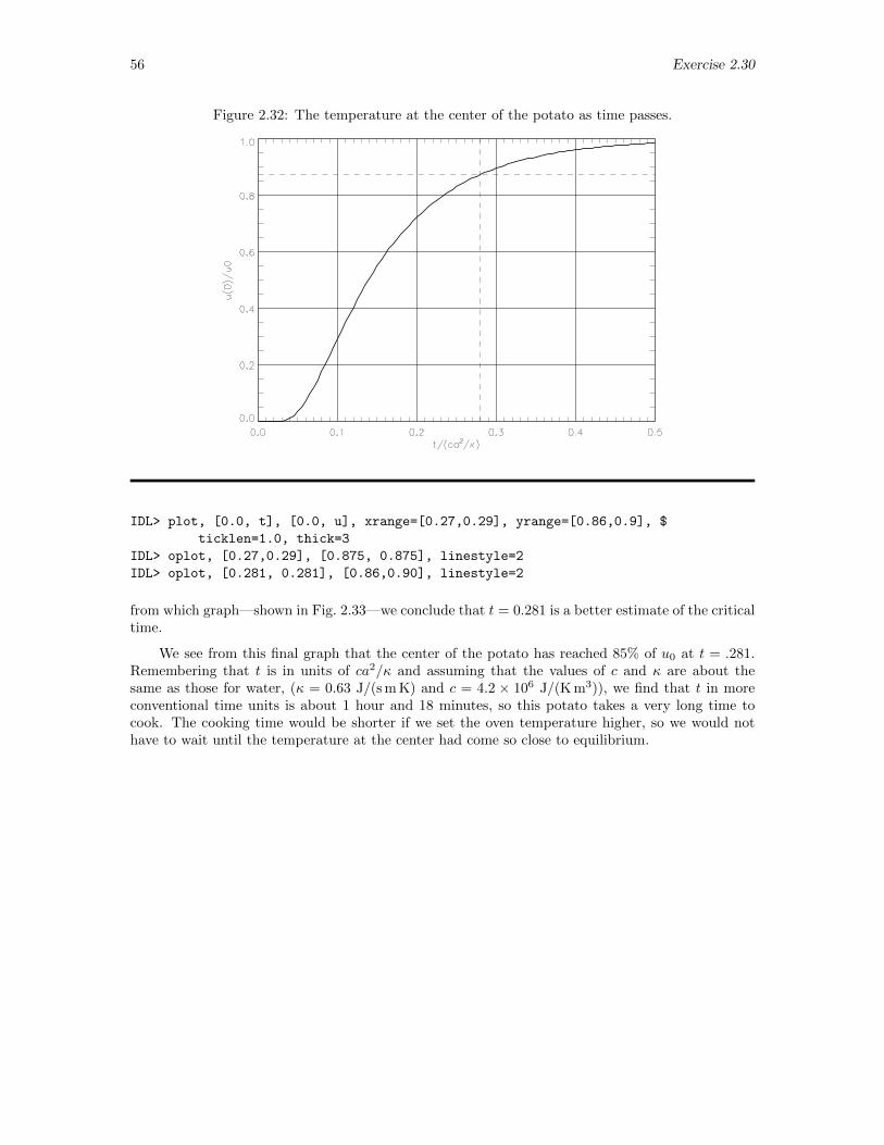
56 Exercise 2.30
Figure 2.32: The temperature at the center of the potato as time passes.
IDL> plot, [0.0, t], [0.0, u], xrange=[0.27,0.29], yrange=[0.86,0.9], $
ticklen=1.0, thick=3
IDL> oplot, [0.27,0.29], [0.875, 0.875], linestyle=2
IDL> oplot, [0.281, 0.281], [0.86,0.90], linestyle=2
from which graph—shown in Fig. 2.33—we conclude that t = 0.281 is a better estimate of the criticaltime.
We see from this final graph that the center of the potato has reached 85% of u0 at t = .281.Remembering that t is in units of ca2/κ and assuming that the values of c and κ are about thesame as those for water, (κ = 0.63 J/(s m K) and c = 4.2 × 10⁶ J/(K m3)), we find that t in moreconventional time units is about 1 hour and 18 minutes, so this potato takes a very long time tocook. The cooking time would be shorter if we set the oven temperature higher, so we would nothave to wait until the temperature at the center had come so close to equilibrium.
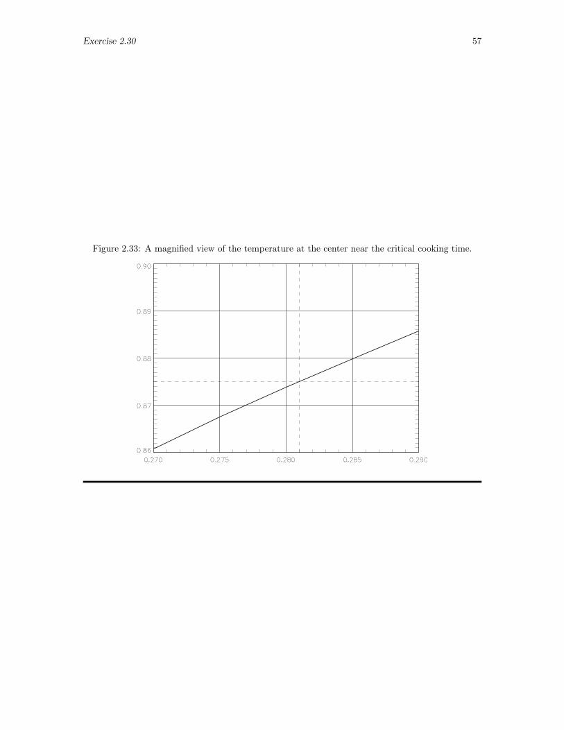
Exercise 2.30 57
Figure 2.33: A magnified view of the temperature at the center near the critical cooking time.
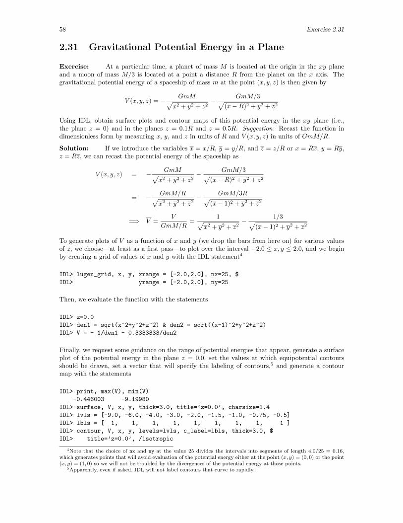
58 Exercise 2.31
2.31 Gravitational Potential Energy in a Plane
Exercise: At a particular time, a planet of mass M is located at the origin in the xy planeand a moon of mass M/3 is located at a point a distance R from the planet on the x axis. Thegravitational potential energy of a spaceship of mass m at the point (x, y, z) is then given by
V (x, y, z) = − GmM√x2 + y2 + z2
− GmM/3√(x−R)2 + y2 + z2
Using IDL, obtain surface plots and contour maps of this potential energy in the xy plane (i.e.,the plane z = 0) and in the planes z = 0.1R and z = 0.5R. Suggestion: Recast the function indimensionless form by measuring x, y, and z in units of R and V (x, y, z) in units of GmM/R.
Solution: If we introduce the variables x = x/R, y = y/R, and z = z/R or x = Rx, y = Ry,z = Rz, we can recast the potential energy of the spaceship as
V (x, y, z) = − GmM√x2 + y2 + z2
− GmM/3√(x−R)2 + y2 + z2
= − GmM/R√x2 + y2 + z2
− GmM/3R√(x− 1)2 + y2 + z2
=⇒ V =V
GmM/R=
1√x2 + y2 + z2
− 1/3√(x− 1)2 + y2 + z2
To generate plots of V as a function of x and y (we drop the bars from here on) for various valuesof z, we choose—at least as a first pass—to plot over the interval −2.0 ≤ x, y ≤ 2.0, and we beginby creating a grid of values of x and y with the IDL statement4
IDL> lugen_grid, x, y, xrange = [-2.0,2.0], nx=25, $
IDL> yrange = [-2.0,2.0], ny=25
Then, we evaluate the function with the statements
IDL> z=0.0
IDL> den1 = sqrt(x^2+y^2+z^2) & den2 = sqrt((x-1)^2+y^2+z^2)
IDL> V = - 1/den1 - 0.3333333/den2
Finally, we request some guidance on the range of potential energies that appear, generate a surfaceplot of the potential energy in the plane z = 0.0, set the values at which equipotential contoursshould be drawn, set a vector that will specify the labeling of contours,5 and generate a contourmap with the statements
IDL> print, max(V), min(V)
-0.446003 -9.19980
IDL> surface, V, x, y, thick=3.0, title=’z=0.0’, charsize=1.4
IDL> lvls = [-9.0, -6.0, -4.0, -3.0, -2.0, -1.5, -1.0, -0.75, -0.5]
IDL> lbls = [ 1, 1, 1, 1, 1, 1, 1, 1, 1 ]
IDL> contour, V, x, y, levels=lvls, c_label=lbls, thick=3.0, $
IDL> title=’z=0.0’, /isotropic
4Note that the choice of nx and ny at the value 25 divides the intervals into segments of length 4.0/25 = 0.16,which generates points that will avoid evaluation of the potential energy either at the point (x, y) = (0, 0) or the point(x, y) = (1, 0) so we will not be troubled by the divergences of the potential energy at those points.
5Apparently, even if asked, IDL will not label contours that curve to rapidly.
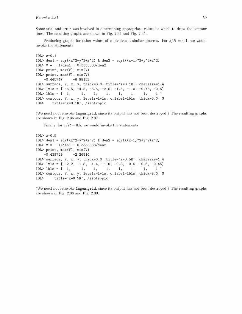
Exercise 2.31 59
Some trial and error was involved in determining appropriate values at which to draw the contourlines. The resulting graphs are shown in Fig. 2.34 and Fig. 2.35.
Producing graphs for other values of z involves a similar process. For z/R = 0.1, we wouldinvoke the statements
IDL> z=0.1
IDL> den1 = sqrt(x^2+y^2+z^2) & den2 = sqrt((x-1)^2+y^2+z^2)
IDL> V = - 1/den1 - 0.3333333/den2
IDL> print, max(V), min(V)
IDL> print, max(V), min(V)
-0.445747 -6.98152
IDL> surface, V, x, y, thick=3.0, title=’z=0.1R’, charsize=1.4
IDL> lvls = [ -6.5, -4.5, -3.5, -2.5, -1.5, -1.0, -0.75, -0.5]
IDL> lbls = [ 1, 1, 1, 1, 1, 1, 1, 1 ]
IDL> contour, V, x, y, levels=lvls, c_label=lbls, thick=3.0, $
IDL> title=’z=0.1R’, /isotropic
(We need not reinvoke lugen grid, since its output has not been destroyed.) The resulting graphsare shown in Fig. 2.36 and Fig. 2.37.
Finally, for z/R = 0.5, we would invoke the statements
IDL> z=0.5
IDL> den1 = sqrt(x^2+y^2+z^2) & den2 = sqrt((x-1)^2+y^2+z^2)
IDL> V = - 1/den1 - 0.3333333/den2
IDL> print, max(V), min(V)
-0.439729 -2.26810
IDL> surface, V, x, y, thick=3.0, title=’z=0.5R’, charsize=1.4
IDL> lvls = [ -2.2, -1.8, -1.4, -1.0, -0.8, -0.6, -0.5, -0.45]
IDL> lbls = [ 1, 1, 1, 1, 1, 1, 1, 1 ]
IDL> contour, V, x, y, levels=lvls, c_label=lbls, thick=3.0, $
IDL> title=’z=0.5R’, /isotropic
(We need not reinvoke lugen grid, since its output has not been destroyed.) The resulting graphsare shown in Fig. 2.38 and Fig. 2.39.
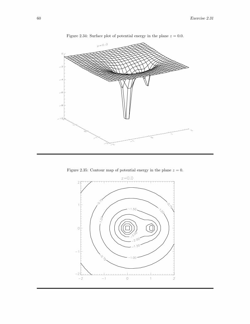
60 Exercise 2.31
Figure 2.34: Surface plot of potential energy in the plane z = 0.0.
Figure 2.35: Contour map of potential energy in the plane z = 0.
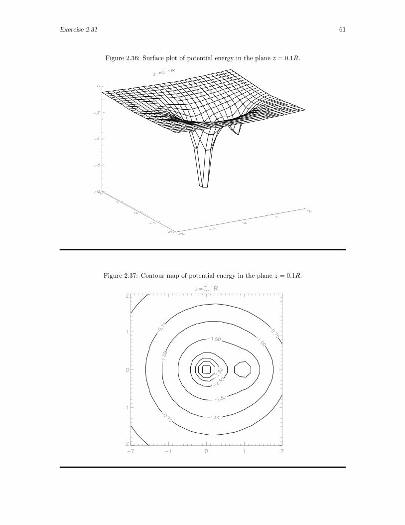
Exercise 2.31 61
Figure 2.36: Surface plot of potential energy in the plane z = 0.1R.
Figure 2.37: Contour map of potential energy in the plane z = 0.1R.
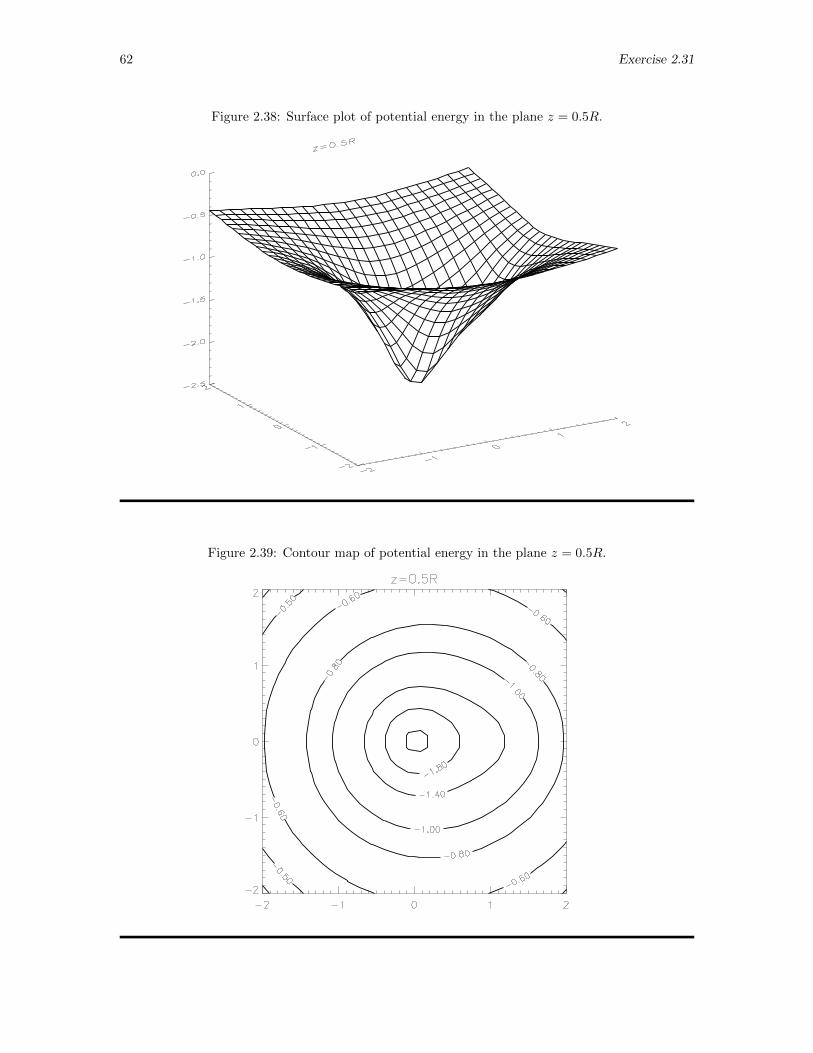
62 Exercise 2.31
Figure 2.38: Surface plot of potential energy in the plane z = 0.5R.
Figure 2.39: Contour map of potential energy in the plane z = 0.5R.
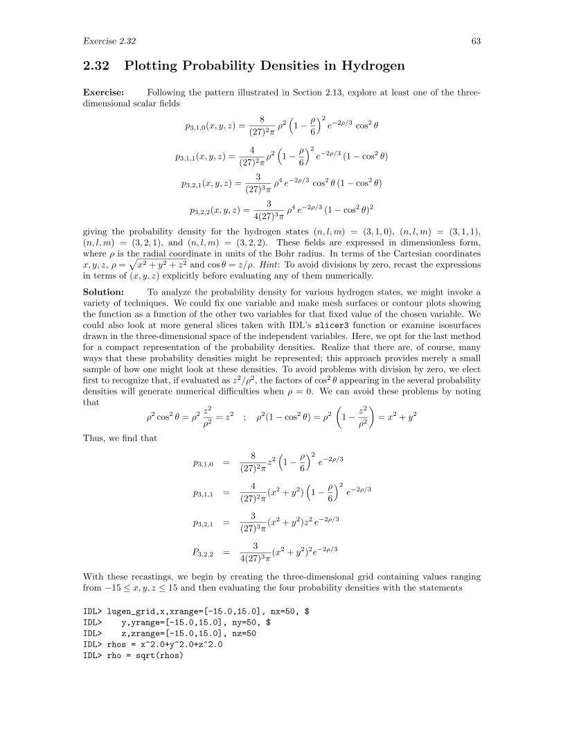
Exercise 2.32 63
2.32 Plotting Probability Densities in Hydrogen
Exercise: Following the pattern illustrated in Section 2.13, explore at least one of the three-dimensional scalar fields
p3,1,0(x, y, z) =8
(27)2πρ2(
1− ρ
6
)2
e−2ρ/3 cos2 θ
p3,1,1(x, y, z) =4
(27)2πρ2(
1− ρ
6
)2
e−2ρ/3 (1− cos2 θ)
p3,2,1(x, y, z) =3
(27)3πρ4 e−2ρ/3 cos2 θ (1− cos2 θ)
p3,2,2(x, y, z) =3
4(27)3πρ4 e−2ρ/3 (1− cos2 θ)2
giving the probability density for the hydrogen states (n, l,m) = (3, 1, 0), (n, l,m) = (3, 1, 1),(n, l,m) = (3, 2, 1), and (n, l,m) = (3, 2, 2). These fields are expressed in dimensionless form,where ρ is the radial coordinate in units of the Bohr radius. In terms of the Cartesian coordinatesx, y, z, ρ =
√x2 + y2 + z2 and cos θ = z/ρ. Hint : To avoid divisions by zero, recast the expressions
in terms of (x, y, z) explicitly before evaluating any of them numerically.
Solution: To analyze the probability density for various hydrogen states, we might invoke avariety of techniques. We could fix one variable and make mesh surfaces or contour plots showingthe function as a function of the other two variables for that fixed value of the chosen variable. Wecould also look at more general slices taken with IDL’s slicer3 function or examine isosurfacesdrawn in the three-dimensional space of the independent variables. Here, we opt for the last methodfor a compact representation of the probability densities. Realize that there are, of course, manyways that these probability densities might be represented; this approach provides merely a smallsample of how one might look at these densities. To avoid problems with division by zero, we electfirst to recognize that, if evaluated as z2/ρ2, the factors of cos2 θ appearing in the several probabilitydensities will generate numerical difficulties when ρ = 0. We can avoid these problems by notingthat
ρ2 cos2 θ = ρ2 z2
ρ2= z2 ; ρ2(1− cos2 θ) = ρ2
(1− z2
ρ2
)= x2 + y2
Thus, we find that
p3,1,0 =8
(27)2πz2(
1− ρ
6
)2
e−2ρ/3
p3,1,1 =4
(27)2π(x2 + y2)
(1− ρ
6
)2
e−2ρ/3
p3,2,1 =3
(27)3π(x2 + y2)z2 e−2ρ/3
P3,2,2 =3
4(27)3π(x2 + y2)2e−2ρ/3
With these recastings, we begin by creating the three-dimensional grid containing values rangingfrom −15 ≤ x, y, z ≤ 15 and then evaluating the four probability densities with the statements
IDL> lugen_grid,x,xrange=[-15.0,15.0], nx=50, $
IDL> y,yrange=[-15.0,15.0], ny=50, $
IDL> z,zrange=[-15.0,15.0], nz=50
IDL> rhos = x^2.0+y^2.0+z^2.0
IDL> rho = sqrt(rhos)
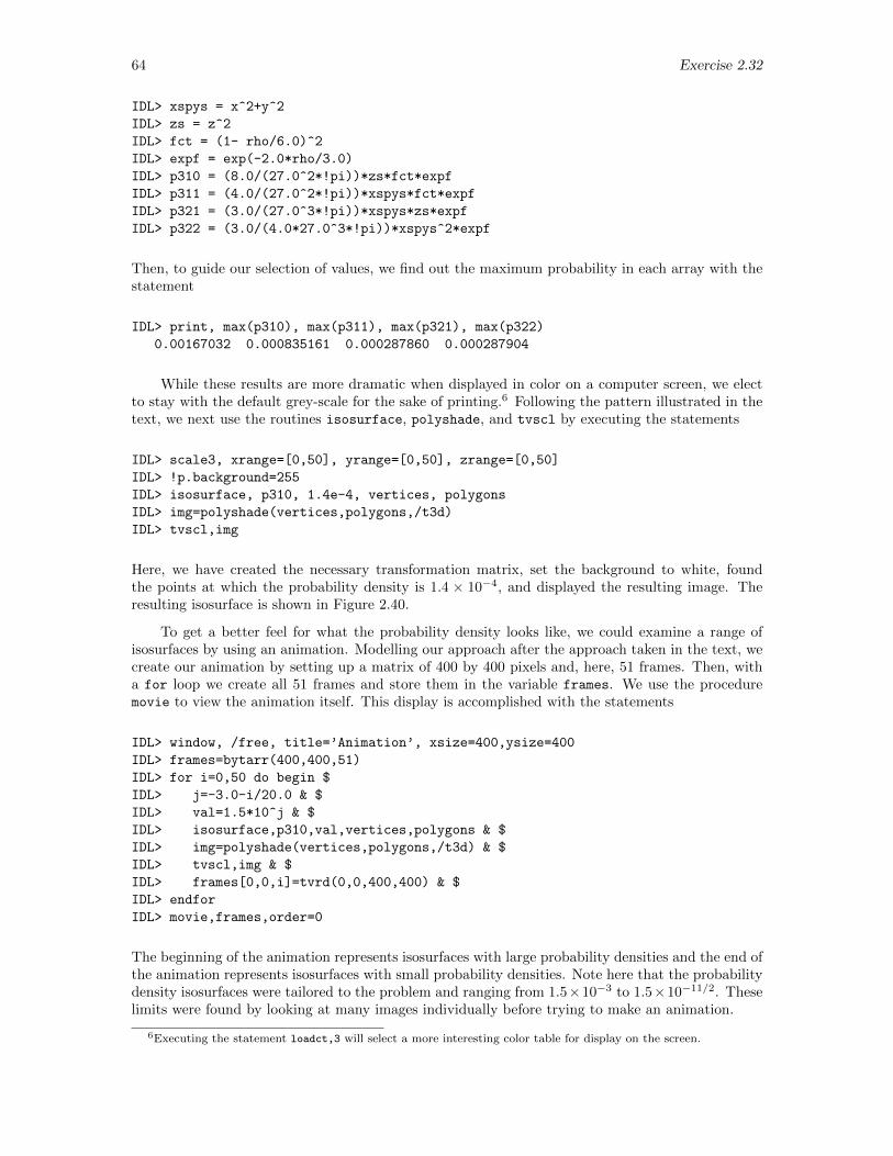
64 Exercise 2.32
IDL> xspys = x^2+y^2
IDL> zs = z^2
IDL> fct = (1- rho/6.0)^2
IDL> expf = exp(-2.0*rho/3.0)
IDL> p310 = (8.0/(27.0^2*!pi))*zs*fct*expf
IDL> p311 = (4.0/(27.0^2*!pi))*xspys*fct*expf
IDL> p321 = (3.0/(27.0^3*!pi))*xspys*zs*expf
IDL> p322 = (3.0/(4.0*27.0^3*!pi))*xspys^2*expf
Then, to guide our selection of values, we find out the maximum probability in each array with thestatement
IDL> print, max(p310), max(p311), max(p321), max(p322)
0.00167032 0.000835161 0.000287860 0.000287904
While these results are more dramatic when displayed in color on a computer screen, we electto stay with the default grey-scale for the sake of printing.6 Following the pattern illustrated in thetext, we next use the routines isosurface, polyshade, and tvscl by executing the statements
IDL> scale3, xrange=[0,50], yrange=[0,50], zrange=[0,50]
IDL> !p.background=255
IDL> isosurface, p310, 1.4e-4, vertices, polygons
IDL> img=polyshade(vertices,polygons,/t3d)
IDL> tvscl,img
Here, we have created the necessary transformation matrix, set the background to white, foundthe points at which the probability density is 1.4 × 10⁻⁴, and displayed the resulting image. Theresulting isosurface is shown in Figure 2.40.
To get a better feel for what the probability density looks like, we could examine a range ofisosurfaces by using an animation. Modelling our approach after the approach taken in the text, wecreate our animation by setting up a matrix of 400 by 400 pixels and, here, 51 frames. Then, witha for loop we create all 51 frames and store them in the variable frames. We use the proceduremovie to view the animation itself. This display is accomplished with the statements
IDL> window, /free, title=’Animation’, xsize=400,ysize=400
IDL> frames=bytarr(400,400,51)
IDL> for i=0,50 do begin $
IDL> j=-3.0-i/20.0 & $
IDL> val=1.5*10^j & $
IDL> isosurface,p310,val,vertices,polygons & $
IDL> img=polyshade(vertices,polygons,/t3d) & $
IDL> tvscl,img & $
IDL> frames[0,0,i]=tvrd(0,0,400,400) & $
IDL> endfor
IDL> movie,frames,order=0
The beginning of the animation represents isosurfaces with large probability densities and the end ofthe animation represents isosurfaces with small probability densities. Note here that the probabilitydensity isosurfaces were tailored to the problem and ranging from 1.5×10⁻³ to 1.5×10⁻¹¹/2. Theselimits were found by looking at many images individually before trying to make an animation.
6Executing the statement loadct,3 will select a more interesting color table for display on the screen.
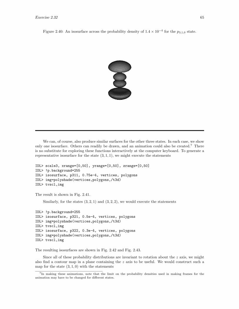
Exercise 2.32 65
Figure 2.40: An isosurface across the probability density of 1.4× 10⁻⁴ for the p3,1,0 state.
We can, of course, also produce similar surfaces for the other three states. In each case, we showonly one isosurface. Others can readily be drawn, and an animation could also be created.7 Thereis no substitute for exploring these functions interactively at the computer keyboard. To generate arepresentative isosurface for the state (3, 1, 1), we might execute the statements
IDL> scale3, xrange=[0,50], yrange=[0,50], zrange=[0,50]
IDL> !p.background=255
IDL> isosurface, p311, 0.75e-4, vertices, polygons
IDL> img=polyshade(vertices,polygons,/t3d)
IDL> tvscl,img
The result is shown in Fig. 2.41.
Similarly, for the states (3, 2, 1) and (3, 2, 2), we would execute the statements
IDL> !p.background=255
IDL> isosurface, p321, 0.5e-4, vertices, polygons
IDL> img=polyshade(vertices,polygons,/t3d)
IDL> tvscl,img
IDL> isosurface, p322, 0.3e-4, vertices, polygons
IDL> img=polyshade(vertices,polygons,/t3d)
IDL> tvscl,img
The resulting isosurfaces are shown in Fig. 2.42 and Fig. 2.43.
Since all of these probability distributions are invariant to rotation about the z axis, we mightalso find a contour map in a plane containing the z axis to be useful. We would construct such amap for the state (3, 1, 0) with the statements
7In making these animations, note that the limit on the probability densities used in making frames for theanimation may have to be changed for different states.
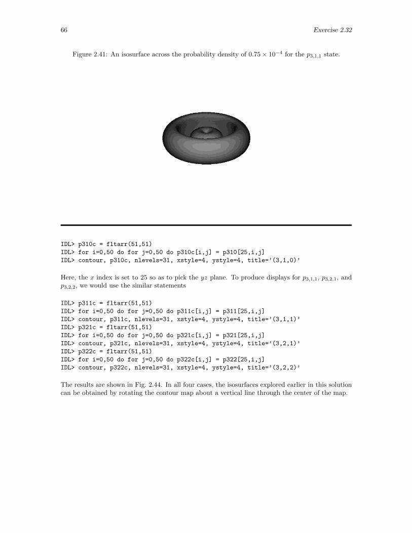
66 Exercise 2.32
Figure 2.41: An isosurface across the probability density of 0.75× 10⁻⁴ for the p3,1,1 state.
IDL> p310c = fltarr(51,51)
IDL> for i=0,50 do for j=0,50 do p310c[i,j] = p310[25,i,j]
IDL> contour, p310c, nlevels=31, xstyle=4, ystyle=4, title=’(3,1,0)’
Here, the x index is set to 25 so as to pick the yz plane. To produce displays for p3,1,1, p3,2,1, andp3,2,2, we would use the similar statements
IDL> p311c = fltarr(51,51)
IDL> for i=0,50 do for j=0,50 do p311c[i,j] = p311[25,i,j]
IDL> contour, p311c, nlevels=31, xstyle=4, ystyle=4, title=’(3,1,1)’
IDL> p321c = fltarr(51,51)
IDL> for i=0,50 do for j=0,50 do p321c[i,j] = p321[25,i,j]
IDL> contour, p321c, nlevels=31, xstyle=4, ystyle=4, title=’(3,2,1)’
IDL> p322c = fltarr(51,51)
IDL> for i=0,50 do for j=0,50 do p322c[i,j] = p322[25,i,j]
IDL> contour, p322c, nlevels=31, xstyle=4, ystyle=4, title=’(3,2,2)’
The results are shown in Fig. 2.44. In all four cases, the isosurfaces explored earlier in this solutioncan be obtained by rotating the contour map about a vertical line through the center of the map.
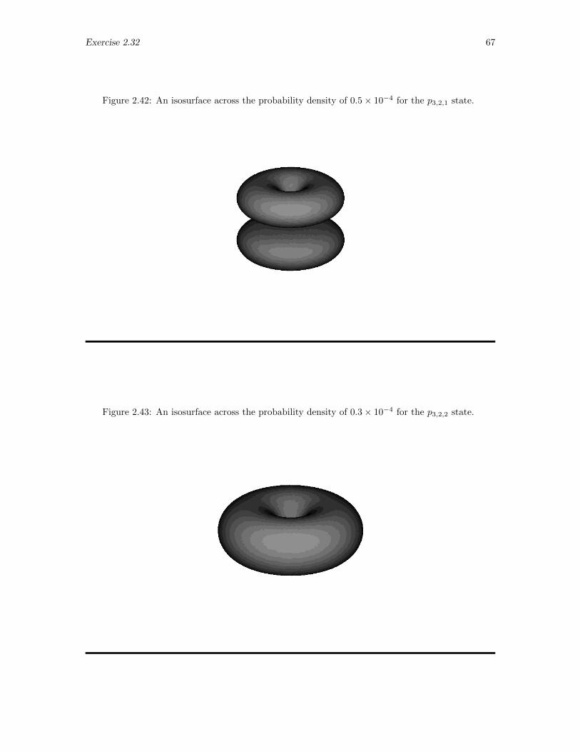
Exercise 2.32 67
Figure 2.42: An isosurface across the probability density of 0.5× 10⁻⁴ for the p3,2,1 state.
Figure 2.43: An isosurface across the probability density of 0.3× 10⁻⁴ for the p3,2,2 state.
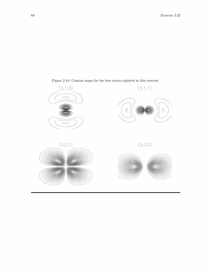
68 Exercise 2.32
Figure 2.44: Contour maps for the four states explored in this exercise.
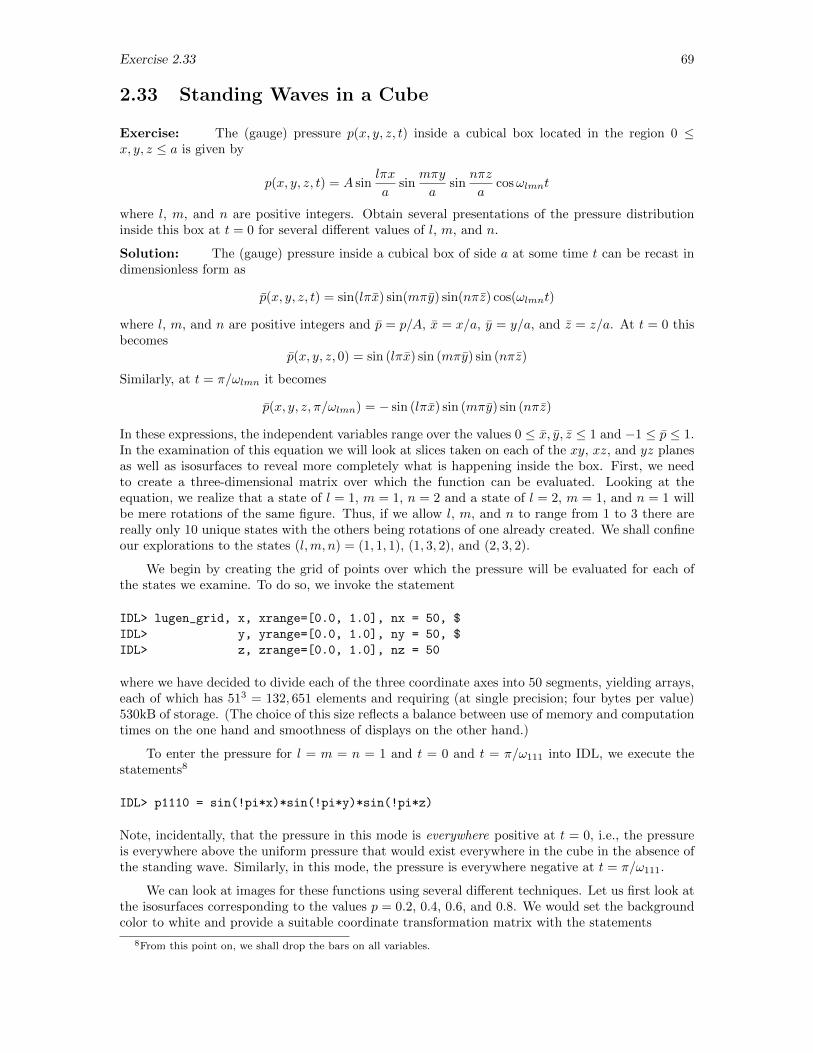
Exercise 2.33 69
2.33 Standing Waves in a Cube
Exercise: The (gauge) pressure p(x, y, z, t) inside a cubical box located in the region 0 ≤x, y, z ≤ a is given by
p(x, y, z, t) = A sinlπx
asin
mπy
asin
nπz
acosωlmnt
where l, m, and n are positive integers. Obtain several presentations of the pressure distributioninside this box at t = 0 for several different values of l, m, and n.
Solution: The (gauge) pressure inside a cubical box of side a at some time t can be recast indimensionless form as
p(x, y, z, t) = sin(lπx) sin(mπy) sin(nπz) cos(ωlmnt)
where l, m, and n are positive integers and p = p/A, x = x/a, y = y/a, and z = z/a. At t = 0 thisbecomes
p(x, y, z, 0) = sin (lπx) sin (mπy) sin (nπz)
Similarly, at t = π/ωlmn it becomes
p(x, y, z, π/ωlmn) = − sin (lπx) sin (mπy) sin (nπz)
In these expressions, the independent variables range over the values 0 ≤ x, y, z ≤ 1 and −1 ≤ p ≤ 1.In the examination of this equation we will look at slices taken on each of the xy, xz, and yz planesas well as isosurfaces to reveal more completely what is happening inside the box. First, we needto create a three-dimensional matrix over which the function can be evaluated. Looking at theequation, we realize that a state of l = 1, m = 1, n = 2 and a state of l = 2, m = 1, and n = 1 willbe mere rotations of the same figure. Thus, if we allow l, m, and n to range from 1 to 3 there arereally only 10 unique states with the others being rotations of one already created. We shall confineour explorations to the states (l,m, n) = (1, 1, 1), (1, 3, 2), and (2, 3, 2).
We begin by creating the grid of points over which the pressure will be evaluated for each ofthe states we examine. To do so, we invoke the statement
IDL> lugen_grid, x, xrange=[0.0, 1.0], nx = 50, $
IDL> y, yrange=[0.0, 1.0], ny = 50, $
IDL> z, zrange=[0.0, 1.0], nz = 50
where we have decided to divide each of the three coordinate axes into 50 segments, yielding arrays,each of which has 513 = 132, 651 elements and requiring (at single precision; four bytes per value)530kB of storage. (The choice of this size reflects a balance between use of memory and computationtimes on the one hand and smoothness of displays on the other hand.)
To enter the pressure for l = m = n = 1 and t = 0 and t = π/ω111 into IDL, we execute thestatements8
IDL> p1110 = sin(!pi*x)*sin(!pi*y)*sin(!pi*z)
Note, incidentally, that the pressure in this mode is everywhere positive at t = 0, i.e., the pressureis everywhere above the uniform pressure that would exist everywhere in the cube in the absence ofthe standing wave. Similarly, in this mode, the pressure is everywhere negative at t = π/ω111.
We can look at images for these functions using several different techniques. Let us first look atthe isosurfaces corresponding to the values p = 0.2, 0.4, 0.6, and 0.8. We would set the backgroundcolor to white and provide a suitable coordinate transformation matrix with the statements
8From this point on, we shall drop the bars on all variables.
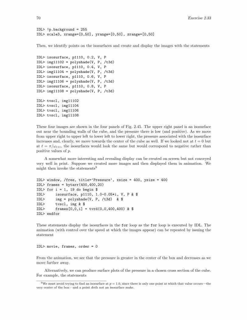
70 Exercise 2.33
IDL> !p.background = 255
IDL> scale3, xrange=[0,50], yrange=[0,50], zrange=[0,50]
Then, we identify points on the isosurfaces and create and display the images with the statements
IDL> isosurface, p1110, 0.2, V, P
IDL> img11102 = polyshade(V, P, /t3d)
IDL> isosurface, p1110, 0.4, V, P
IDL> img11104 = polyshade(V, P, /t3d)
IDL> isosurface, p1110, 0.6, V, P
IDL> img11106 = polyshade(V, P, /t3d)
IDL> isosurface, p1110, 0.8, V, P
IDL> img11108 = polyshade(V, P, /t3d)
IDL> tvscl, img11102
IDL> tvscl, img11104
IDL> tvscl, img11106
IDL> tvscl, img11108
These four images are shown in the four panels of Fig. 2.45. The upper right panel is an isosurfaceout near the bounding walls of the cube, and the pressure there is low (and positive). As we movefrom upper right to upper left to lower left to lower right, the pressure associated with the isosurfaceincreases and, clearly, we move towards the center of the cube as well. If we looked not at t = 0 butat t = π/ω111, the isosurfaces would look the same but would correspond to negative rather thanpositive values of p.
A somewhat more interesting and revealing display can be created on screen but not conveyedvery well in print. Suppose we created more images and then displayed them in animation. Wemight then invoke the statements9
IDL> window, /free, title=’Pressure’, xsize = 400, ysize = 400
IDL> frames = bytarr(400,400,20)
IDL> for i = 1, 19 do begin $
IDL> isosurface, p1110, 1.0-0.05*i, V, P & $
IDL> img = polyshade(V, P, /t3d) & $
IDL> tvscl, img & $
IDL> frames[0,0,i] = tvrd(0,0,400,400) & $
IDL> endfor
These statements display the isosurfaces in the for loop as the for loop is executed by IDL. Theanimation (with control over the speed at which the images appear) can be repeated by issuing thestatement
IDL> movie, frames, order = 0
From the animation, we see that the pressure is greater in the center of the box and decreases as wemove farther away.
Alternatively, we can produce surface plots of the pressure in a chosen cross section of the cube.For example, the statements
9We must avoid trying to find an isosurface at p = 1.0, since there is only one point at which that value occurs—thevery center of the box—and a point doth not an isosurface make.
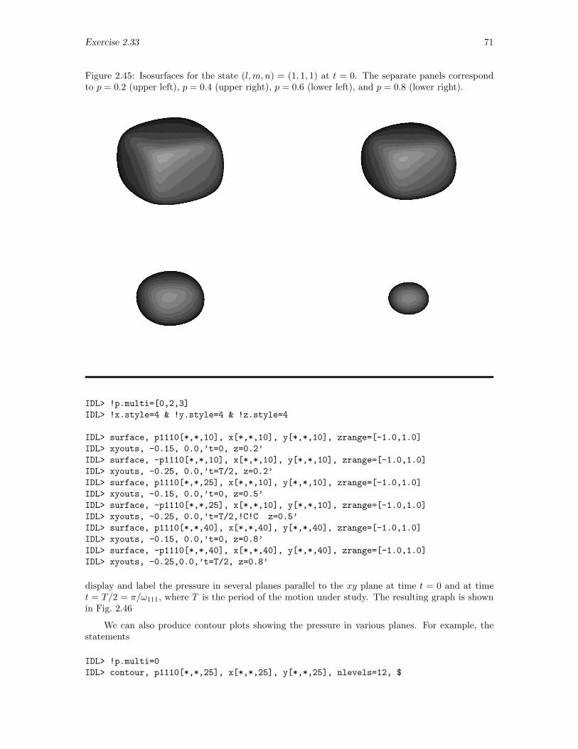
Exercise 2.33 71
Figure 2.45: Isosurfaces for the state (l,m, n) = (1, 1, 1) at t = 0. The separate panels correspondto p = 0.2 (upper left), p = 0.4 (upper right), p = 0.6 (lower left), and p = 0.8 (lower right).
IDL> !p.multi=[0,2,3]
IDL> !x.style=4 & !y.style=4 & !z.style=4
IDL> surface, p1110[*,*,10], x[*,*,10], y[*,*,10], zrange=[-1.0,1.0]
IDL> xyouts, -0.15, 0.0,’t=0, z=0.2’
IDL> surface, -p1110[*,*,10], x[*,*,10], y[*,*,10], zrange=[-1.0,1.0]
IDL> xyouts, -0.25, 0.0,’t=T/2, z=0.2’
IDL> surface, p1110[*,*,25], x[*,*,10], y[*,*,10], zrange=[-1.0,1.0]
IDL> xyouts, -0.15, 0.0,’t=0, z=0.5’
IDL> surface, -p1110[*,*,25], x[*,*,10], y[*,*,10], zrange=[-1.0,1.0]
IDL> xyouts, -0.25, 0.0,’t=T/2,!C!C z=0.5’
IDL> surface, p1110[*,*,40], x[*,*,40], y[*,*,40], zrange=[-1.0,1.0]
IDL> xyouts, -0.15, 0.0,’t=0, z=0.8’
IDL> surface, -p1110[*,*,40], x[*,*,40], y[*,*,40], zrange=[-1.0,1.0]
IDL> xyouts, -0.25,0.0,’t=T/2, z=0.8’
display and label the pressure in several planes parallel to the xy plane at time t = 0 and at timet = T/2 = π/ω111, where T is the period of the motion under study. The resulting graph is shownin Fig. 2.46
We can also produce contour plots showing the pressure in various planes. For example, thestatements
IDL> !p.multi=0
IDL> contour, p1110[*,*,25], x[*,*,25], y[*,*,25], nlevels=12, $
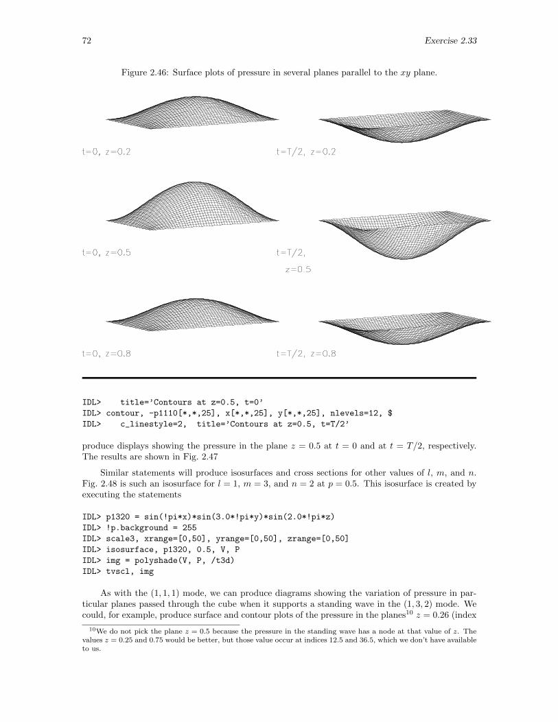
72 Exercise 2.33
Figure 2.46: Surface plots of pressure in several planes parallel to the xy plane.
IDL> title=’Contours at z=0.5, t=0’
IDL> contour, -p1110[*,*,25], x[*,*,25], y[*,*,25], nlevels=12, $
IDL> c_linestyle=2, title=’Contours at z=0.5, t=T/2’
produce displays showing the pressure in the plane z = 0.5 at t = 0 and at t = T/2, respectively.The results are shown in Fig. 2.47
Similar statements will produce isosurfaces and cross sections for other values of l, m, and n.Fig. 2.48 is such an isosurface for l = 1, m = 3, and n = 2 at p = 0.5. This isosurface is created byexecuting the statements
IDL> p1320 = sin(!pi*x)*sin(3.0*!pi*y)*sin(2.0*!pi*z)
IDL> !p.background = 255
IDL> scale3, xrange=[0,50], yrange=[0,50], zrange=[0,50]
IDL> isosurface, p1320, 0.5, V, P
IDL> img = polyshade(V, P, /t3d)
IDL> tvscl, img
As with the (1, 1, 1) mode, we can produce diagrams showing the variation of pressure in par-ticular planes passed through the cube when it supports a standing wave in the (1, 3, 2) mode. Wecould, for example, produce surface and contour plots of the pressure in the planes10 z = 0.26 (index
10We do not pick the plane z = 0.5 because the pressure in the standing wave has a node at that value of z. Thevalues z = 0.25 and 0.75 would be better, but those value occur at indices 12.5 and 36.5, which we don’t have availableto us.
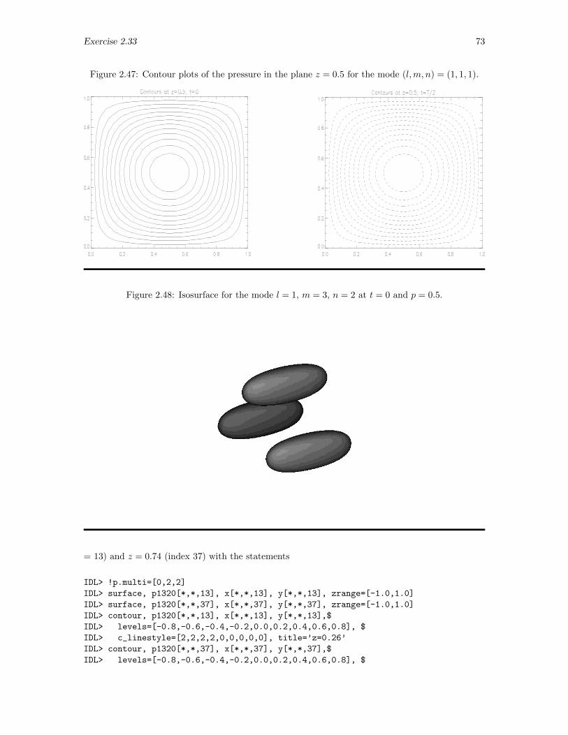
Exercise 2.33 73
Figure 2.47: Contour plots of the pressure in the plane z = 0.5 for the mode (l,m, n) = (1, 1, 1).
Figure 2.48: Isosurface for the mode l = 1, m = 3, n = 2 at t = 0 and p = 0.5.
= 13) and z = 0.74 (index 37) with the statements
IDL> !p.multi=[0,2,2]
IDL> surface, p1320[*,*,13], x[*,*,13], y[*,*,13], zrange=[-1.0,1.0]
IDL> surface, p1320[*,*,37], x[*,*,37], y[*,*,37], zrange=[-1.0,1.0]
IDL> contour, p1320[*,*,13], x[*,*,13], y[*,*,13],$
IDL> levels=[-0.8,-0.6,-0.4,-0.2,0.0,0.2,0.4,0.6,0.8], $
IDL> c_linestyle=[2,2,2,2,0,0,0,0,0], title=’z=0.26’
IDL> contour, p1320[*,*,37], x[*,*,37], y[*,*,37],$
IDL> levels=[-0.8,-0.6,-0.4,-0.2,0.0,0.2,0.4,0.6,0.8], $
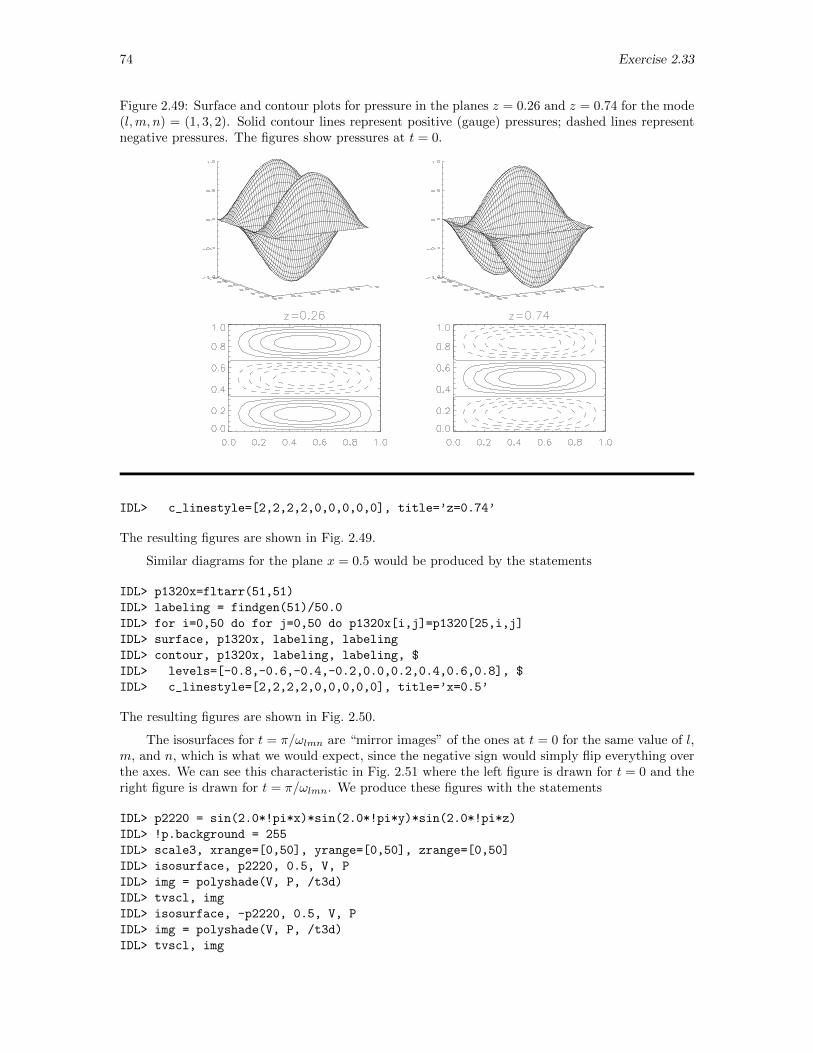
74 Exercise 2.33
Figure 2.49: Surface and contour plots for pressure in the planes z = 0.26 and z = 0.74 for the mode(l,m, n) = (1, 3, 2). Solid contour lines represent positive (gauge) pressures; dashed lines representnegative pressures. The figures show pressures at t = 0.
IDL> c_linestyle=[2,2,2,2,0,0,0,0,0], title=’z=0.74’
The resulting figures are shown in Fig. 2.49.
Similar diagrams for the plane x = 0.5 would be produced by the statements
IDL> p1320x=fltarr(51,51)
IDL> labeling = findgen(51)/50.0
IDL> for i=0,50 do for j=0,50 do p1320x[i,j]=p1320[25,i,j]
IDL> surface, p1320x, labeling, labeling
IDL> contour, p1320x, labeling, labeling, $
IDL> levels=[-0.8,-0.6,-0.4,-0.2,0.0,0.2,0.4,0.6,0.8], $
IDL> c_linestyle=[2,2,2,2,0,0,0,0,0], title=’x=0.5’
The resulting figures are shown in Fig. 2.50.
The isosurfaces for t = π/ωlmn are “mirror images” of the ones at t = 0 for the same value of l,m, and n, which is what we would expect, since the negative sign would simply flip everything overthe axes. We can see this characteristic in Fig. 2.51 where the left figure is drawn for t = 0 and theright figure is drawn for t = π/ωlmn. We produce these figures with the statements
IDL> p2220 = sin(2.0*!pi*x)*sin(2.0*!pi*y)*sin(2.0*!pi*z)
IDL> !p.background = 255
IDL> scale3, xrange=[0,50], yrange=[0,50], zrange=[0,50]
IDL> isosurface, p2220, 0.5, V, P
IDL> img = polyshade(V, P, /t3d)
IDL> tvscl, img
IDL> isosurface, -p2220, 0.5, V, P
IDL> img = polyshade(V, P, /t3d)
IDL> tvscl, img
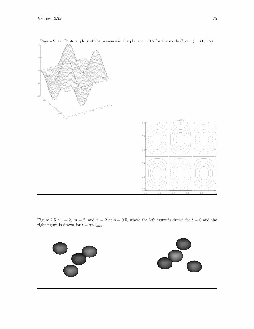
Exercise 2.33 75
Figure 2.50: Contour plots of the pressure in the plane x = 0.5 for the mode (l,m, n) = (1, 3, 2).
Figure 2.51: l = 2, m = 2, and n = 2 at p = 0.5, where the left figure is drawn for t = 0 and theright figure is drawn for t = π/ωlmn.
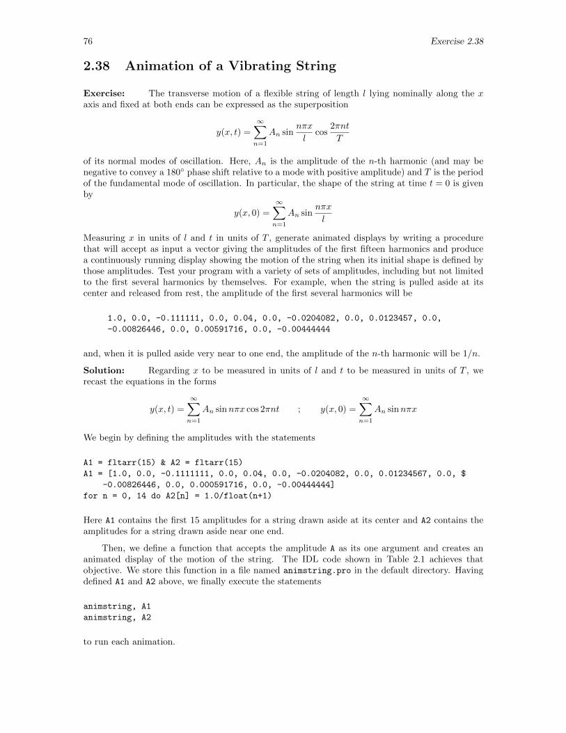
76 Exercise 2.38
2.38 Animation of a Vibrating String
Exercise: The transverse motion of a flexible string of length l lying nominally along the xaxis and fixed at both ends can be expressed as the superposition
y(x, t) =
∞∑n=1
An sinnπx
lcos
2πnt
T
of its normal modes of oscillation. Here, An is the amplitude of the n-th harmonic (and may benegative to convey a 180 phase shift relative to a mode with positive amplitude) and T is the periodof the fundamental mode of oscillation. In particular, the shape of the string at time t = 0 is givenby
y(x, 0) =
∞∑n=1
An sinnπx
l
Measuring x in units of l and t in units of T , generate animated displays by writing a procedurethat will accept as input a vector giving the amplitudes of the first fifteen harmonics and producea continuously running display showing the motion of the string when its initial shape is defined bythose amplitudes. Test your program with a variety of sets of amplitudes, including but not limitedto the first several harmonics by themselves. For example, when the string is pulled aside at itscenter and released from rest, the amplitude of the first several harmonics will be
1.0, 0.0, -0.111111, 0.0, 0.04, 0.0, -0.0204082, 0.0, 0.0123457, 0.0,
-0.00826446, 0.0, 0.00591716, 0.0, -0.00444444
and, when it is pulled aside very near to one end, the amplitude of the n-th harmonic will be 1/n.
Solution: Regarding x to be measured in units of l and t to be measured in units of T , werecast the equations in the forms
y(x, t) =
∞∑n=1
An sinnπx cos 2πnt ; y(x, 0) =
∞∑n=1
An sinnπx
We begin by defining the amplitudes with the statements
A1 = fltarr(15) & A2 = fltarr(15)
A1 = [1.0, 0.0, -0.1111111, 0.0, 0.04, 0.0, -0.0204082, 0.0, 0.01234567, 0.0, $
-0.00826446, 0.0, 0.000591716, 0.0, -0.00444444]
for n = 0, 14 do A2[n] = 1.0/float(n+1)
Here A1 contains the first 15 amplitudes for a string drawn aside at its center and A2 contains theamplitudes for a string drawn aside near one end.
Then, we define a function that accepts the amplitude A as its one argument and creates ananimated display of the motion of the string. The IDL code shown in Table 2.1 achieves thatobjective. We store this function in a file named animstring.pro in the default directory. Havingdefined A1 and A2 above, we finally execute the statements
animstring, A1
animstring, A2
to run each animation.
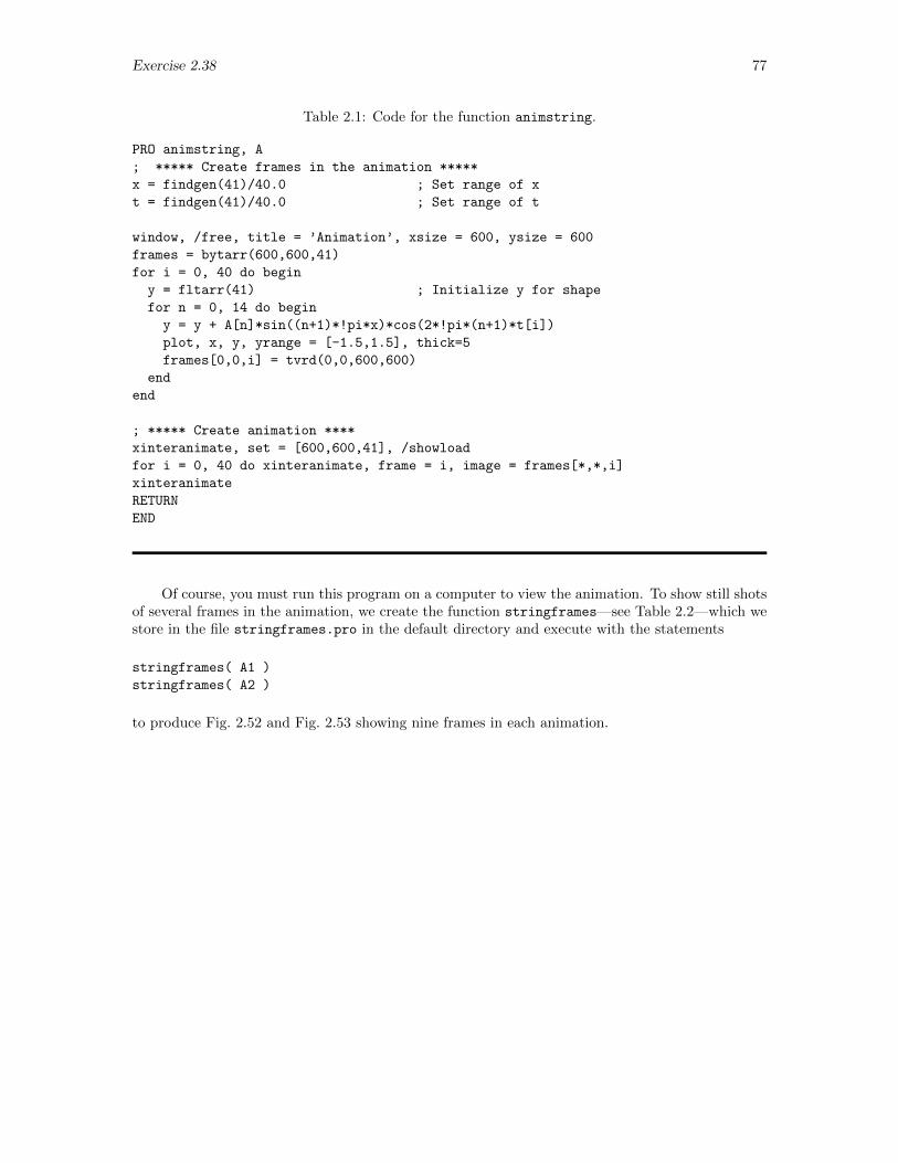
Exercise 2.38 77
Table 2.1: Code for the function animstring.
PRO animstring, A
; ***** Create frames in the animation *****
x = findgen(41)/40.0 ; Set range of x
t = findgen(41)/40.0 ; Set range of t
window, /free, title = ’Animation’, xsize = 600, ysize = 600
frames = bytarr(600,600,41)
for i = 0, 40 do begin
y = fltarr(41) ; Initialize y for shape
for n = 0, 14 do begin
y = y + A[n]*sin((n+1)*!pi*x)*cos(2*!pi*(n+1)*t[i])
plot, x, y, yrange = [-1.5,1.5], thick=5
frames[0,0,i] = tvrd(0,0,600,600)
end
end
; ***** Create animation ****
xinteranimate, set = [600,600,41], /showload
for i = 0, 40 do xinteranimate, frame = i, image = frames[*,*,i]
xinteranimate
RETURN
END
Of course, you must run this program on a computer to view the animation. To show still shotsof several frames in the animation, we create the function stringframes—see Table 2.2—which westore in the file stringframes.pro in the default directory and execute with the statements
stringframes( A1 )
stringframes( A2 )
to produce Fig. 2.52 and Fig. 2.53 showing nine frames in each animation.
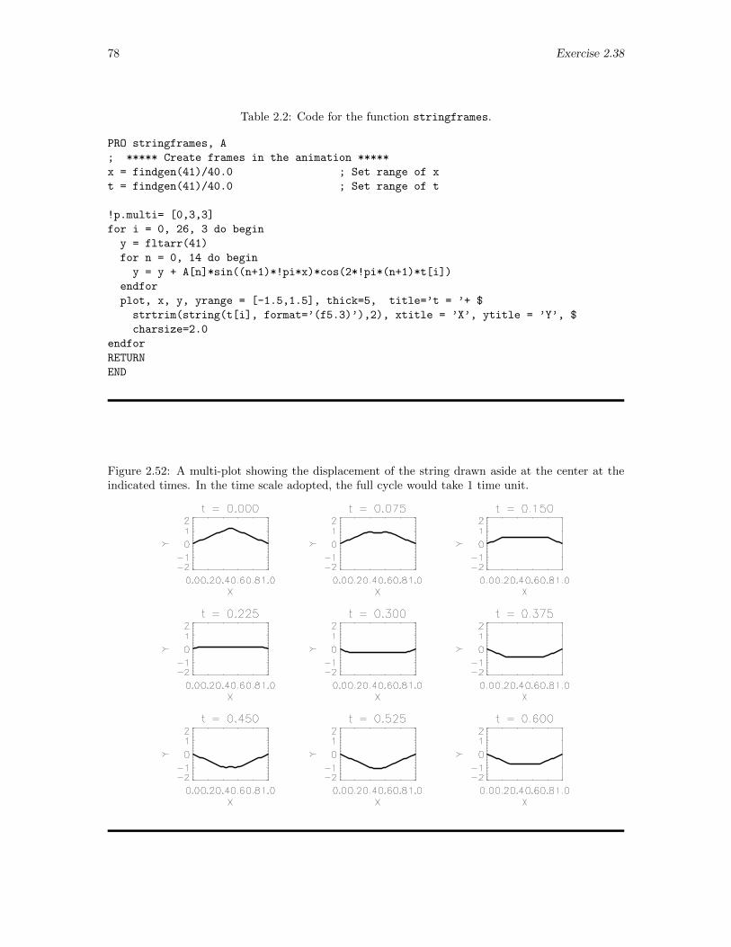
78 Exercise 2.38
Table 2.2: Code for the function stringframes.
PRO stringframes, A
; ***** Create frames in the animation *****
x = findgen(41)/40.0 ; Set range of x
t = findgen(41)/40.0 ; Set range of t
!p.multi= [0,3,3]
for i = 0, 26, 3 do begin
y = fltarr(41)
for n = 0, 14 do begin
y = y + A[n]*sin((n+1)*!pi*x)*cos(2*!pi*(n+1)*t[i])
endfor
plot, x, y, yrange = [-1.5,1.5], thick=5, title=’t = ’+ $
strtrim(string(t[i], format=’(f5.3)’),2), xtitle = ’X’, ytitle = ’Y’, $
charsize=2.0
endfor
RETURN
END
Figure 2.52: A multi-plot showing the displacement of the string drawn aside at the center at theindicated times. In the time scale adopted, the full cycle would take 1 time unit.
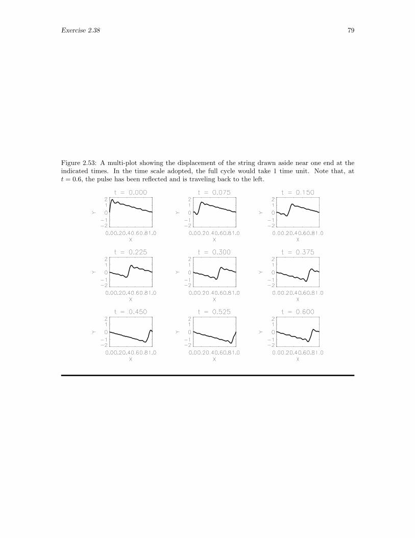
Exercise 2.38 79
Figure 2.53: A multi-plot showing the displacement of the string drawn aside near one end at theindicated times. In the time scale adopted, the full cycle would take 1 time unit. Note that, att = 0.6, the pulse has been reflected and is traveling back to the left.
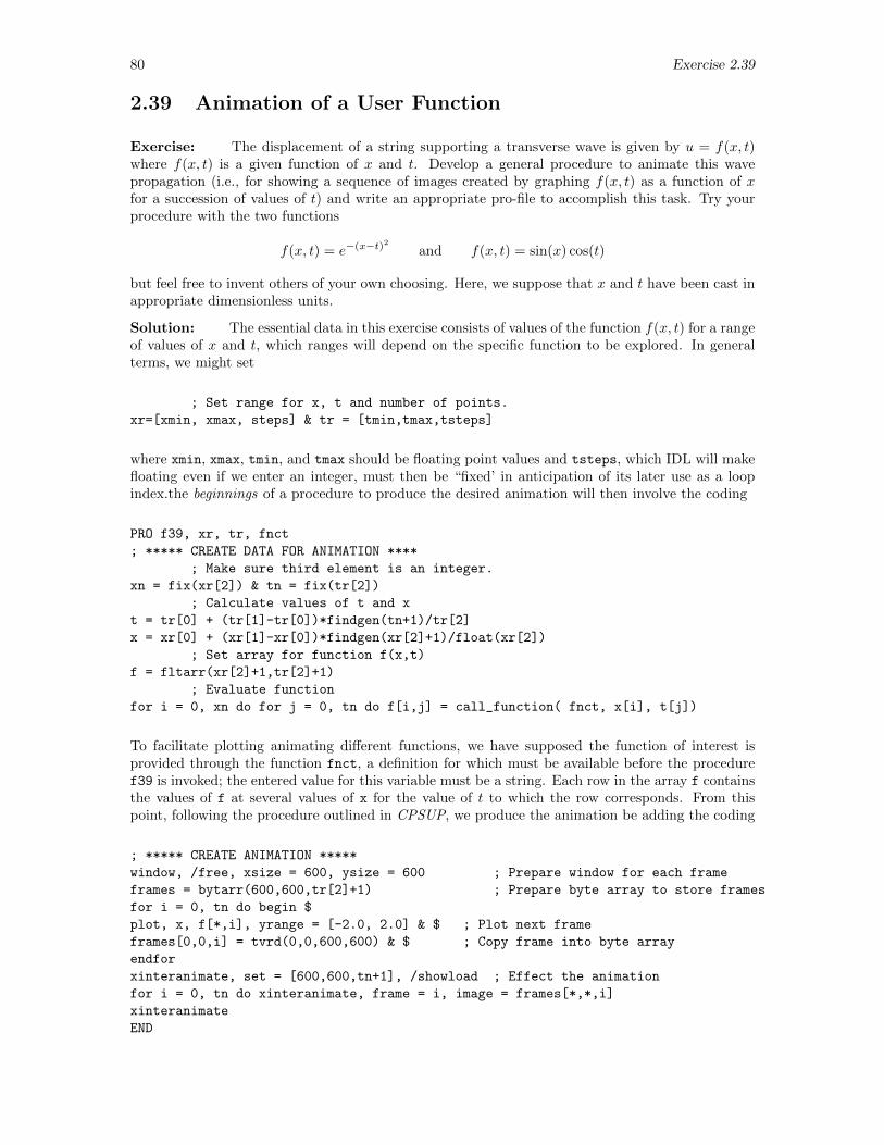
80 Exercise 2.39
2.39 Animation of a User Function
Exercise: The displacement of a string supporting a transverse wave is given by u = f(x, t)where f(x, t) is a given function of x and t. Develop a general procedure to animate this wavepropagation (i.e., for showing a sequence of images created by graphing f(x, t) as a function of xfor a succession of values of t) and write an appropriate pro-file to accomplish this task. Try yourprocedure with the two functions
f(x, t) = e−(x−t)2 and f(x, t) = sin(x) cos(t)
but feel free to invent others of your own choosing. Here, we suppose that x and t have been cast inappropriate dimensionless units.
Solution: The essential data in this exercise consists of values of the function f(x, t) for a rangeof values of x and t, which ranges will depend on the specific function to be explored. In generalterms, we might set
; Set range for x, t and number of points.
xr=[xmin, xmax, steps] & tr = [tmin,tmax,tsteps]
where xmin, xmax, tmin, and tmax should be floating point values and tsteps, which IDL will makefloating even if we enter an integer, must then be “fixed’ in anticipation of its later use as a loopindex.the beginnings of a procedure to produce the desired animation will then involve the coding
PRO f39, xr, tr, fnct
; ***** CREATE DATA FOR ANIMATION ****
; Make sure third element is an integer.
xn = fix(xr[2]) & tn = fix(tr[2])
; Calculate values of t and x
t = tr[0] + (tr[1]-tr[0])*findgen(tn+1)/tr[2]
x = xr[0] + (xr[1]-xr[0])*findgen(xr[2]+1)/float(xr[2])
; Set array for function f(x,t)
f = fltarr(xr[2]+1,tr[2]+1)
; Evaluate function
for i = 0, xn do for j = 0, tn do f[i,j] = call_function( fnct, x[i], t[j])
To facilitate plotting animating different functions, we have supposed the function of interest isprovided through the function fnct, a definition for which must be available before the proceduref39 is invoked; the entered value for this variable must be a string. Each row in the array f containsthe values of f at several values of x for the value of t to which the row corresponds. From thispoint, following the procedure outlined in CPSUP, we produce the animation be adding the coding
; ***** CREATE ANIMATION *****
window, /free, xsize = 600, ysize = 600 ; Prepare window for each frame
frames = bytarr(600,600,tr[2]+1) ; Prepare byte array to store frames
for i = 0, tn do begin $
plot, x, f[*,i], yrange = [-2.0, 2.0] & $ ; Plot next frame
frames[0,0,i] = tvrd(0,0,600,600) & $ ; Copy frame into byte array
endfor
xinteranimate, set = [600,600,tn+1], /showload ; Effect the animation
for i = 0, tn do xinteranimate, frame = i, image = frames[*,*,i]
xinteranimate
END
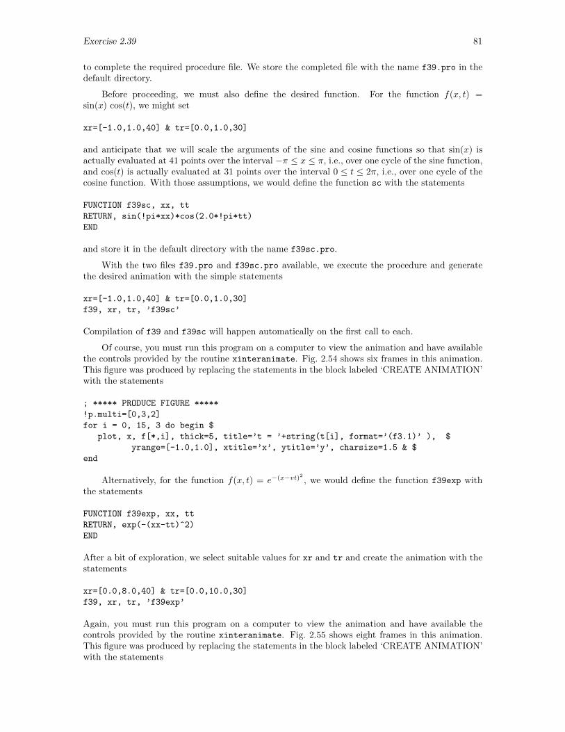
Exercise 2.39 81
to complete the required procedure file. We store the completed file with the name f39.pro in thedefault directory.
Before proceeding, we must also define the desired function. For the function f(x, t) =sin(x) cos(t), we might set
xr=[-1.0,1.0,40] & tr=[0.0,1.0,30]
and anticipate that we will scale the arguments of the sine and cosine functions so that sin(x) isactually evaluated at 41 points over the interval −π ≤ x ≤ π, i.e., over one cycle of the sine function,and cos(t) is actually evaluated at 31 points over the interval 0 ≤ t ≤ 2π, i.e., over one cycle of thecosine function. With those assumptions, we would define the function sc with the statements
FUNCTION f39sc, xx, tt
RETURN, sin(!pi*xx)*cos(2.0*!pi*tt)
END
and store it in the default directory with the name f39sc.pro.
With the two files f39.pro and f39sc.pro available, we execute the procedure and generatethe desired animation with the simple statements
xr=[-1.0,1.0,40] & tr=[0.0,1.0,30]
f39, xr, tr, ’f39sc’
Compilation of f39 and f39sc will happen automatically on the first call to each.
Of course, you must run this program on a computer to view the animation and have availablethe controls provided by the routine xinteranimate. Fig. 2.54 shows six frames in this animation.This figure was produced by replacing the statements in the block labeled ‘CREATE ANIMATION’with the statements
; ***** PRODUCE FIGURE *****
!p.multi=[0,3,2]
for i = 0, 15, 3 do begin $
plot, x, f[*,i], thick=5, title=’t = ’+string(t[i], format=’(f3.1)’ ), $
yrange=[-1.0,1.0], xtitle=’x’, ytitle=’y’, charsize=1.5 & $
end
Alternatively, for the function f(x, t) = e−(x−vt)2 , we would define the function f39exp withthe statements
FUNCTION f39exp, xx, tt
RETURN, exp(-(xx-tt)^2)
END
After a bit of exploration, we select suitable values for xr and tr and create the animation with thestatements
xr=[0.0,8.0,40] & tr=[0.0,10.0,30]
f39, xr, tr, ’f39exp’
Again, you must run this program on a computer to view the animation and have available thecontrols provided by the routine xinteranimate. Fig. 2.55 shows eight frames in this animation.This figure was produced by replacing the statements in the block labeled ‘CREATE ANIMATION’with the statements
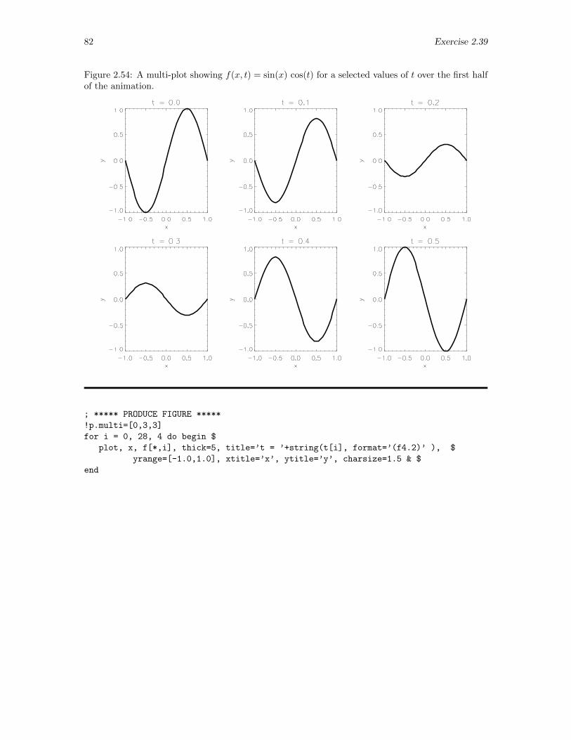
82 Exercise 2.39
Figure 2.54: A multi-plot showing f(x, t) = sin(x) cos(t) for a selected values of t over the first halfof the animation.
; ***** PRODUCE FIGURE *****
!p.multi=[0,3,3]
for i = 0, 28, 4 do begin $
plot, x, f[*,i], thick=5, title=’t = ’+string(t[i], format=’(f4.2)’ ), $
yrange=[-1.0,1.0], xtitle=’x’, ytitle=’y’, charsize=1.5 & $
end
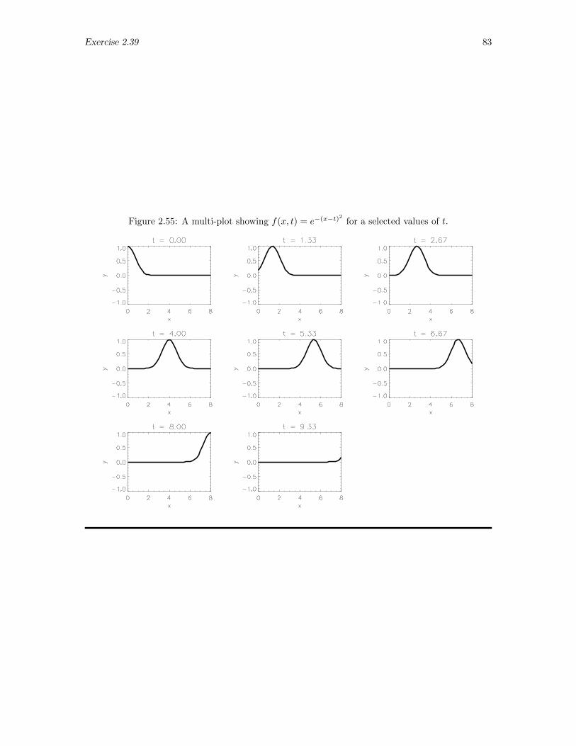
Exercise 2.39 83
Figure 2.55: A multi-plot showing f(x, t) = e−(x−t)2 for a selected values of t.
84 Exercise 2.40
2.40 Animation of a Square Membrane
Exercise: The displacement of a square membrane extending over the region 0 ≤ x, y ≤ awhen it is oscillating in its m,n normal mode is given by
u(x, y, t) = A sin(mπx
a
)sin(nπy
a
)cos(ωmnt)
where ωmn = (cπ/a)√m2 + n2, c being the speed of propagation of the waves in the membrane.
Write a procedure pro-file in IDL to animate the motion of this drumhead for a user-selected mode(user-selected values of m and n). Suggestions: (1) Express x and y in units of a and u in units ofA so the graphs you produce will show u/A above the (x/a)(y/a)-plane. (2) Review the discussionin the last paragraph of Section 2.15.
Solution: Given the above equation, we can immediately begin writing a pro-file that willanimate this motion. One condition is that the user is to input the values of m and n, so m andn must be included as arguments. Likewise, from looking at the hints we can also substitute thefollowing: x = x/a, y = y/a, and u = u/A, which leads to the new (and plottable) equation
u(x, y, t) = sin(mπx) sin(nπy) cos(ωmnt)
in dimensionless form. Notice that, although t still exists in the equation, the term (cπ)/a in ωmnis in units of inverse time (frequency), so the units cancel out completely.
Although u is given as a three-dimensional function, it is here convenient to think of it as asuccession of xy-planes, one for each value of t. Thus, we c an utilize lugen grid to fee us an arrayof x and y coordinates, evaluate the xy factors in the function, and then for a range of values of tcalculate the value of the function in the xy-plane for each t with the statements
PRO f40, m, n ; Define procedure
nx = 50 & ny = 50 ; Set size of grid
lugen_grid, x, xrange = [0.0, 1.0], nx = nx, $ ; Create grid
y, yrange = [0.0, 1.0], ny = ny
t = findgen(41)/40.0 ; Set times for solutions
disp = fltarr(nx+1, ny+1, 41) ; Create array for images
u = sin(m*!pi*x)*sin(n*!pi*y) ; Evaluate initial shape
for i = 0, 40 do disp[*,*,i] = u*cos(2*!pi*t[i]) ; Calculate shape for each t
window, /free, xsize = 600, ysize = 600 ; Create window for display
frames = bytarr(600,600,41) ; Create byte file for images
for i = 0, 40 do begin $
shade_surf, disp[*,*,i], zrange = [-1.0, 1.0] & $ ; Display each image
frames[0,0,i] = tvrd(0,0,600,600) & $ ; Read image into byte array
endfor
xinteranimate, set = [600,600,41], /showload ; Create animation
for i = 0, 40 do xinteranimate, frame = i, image = frames[*,*,i]
xinteranimate
END
which follow the pattern illustrated in Section 2.15 in CPSUP .
While the animation can be viewed only on a computer screen, several frames from that ani-mation for the [2, 3] mode are recorded in Fig. 2.56. For the sake of completeness, we note that thisfigure was created with the code
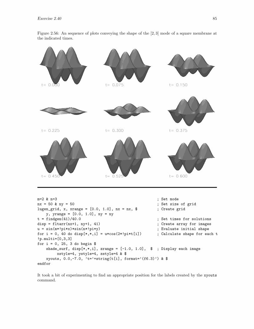
Exercise 2.40 85
Figure 2.56: An sequence of plots conveying the shape of the [2, 3] mode of a square membrane atthe indicated times.
m=2 & n=3 ; Set mode
nx = 50 & ny = 50 ; Set size of grid
lugen_grid, x, xrange = [0.0, 1.0], nx = nx, $ ; Create grid
y, yrange = [0.0, 1.0], ny = ny
t = findgen(41)/40.0 ; Set times for solutions
disp = fltarr(nx+1, ny+1, 41) ; Create array for images
u = sin(m*!pi*x)*sin(n*!pi*y) ; Evaluate initial shape
for i = 0, 40 do disp[*,*,i] = u*cos(2*!pi*t[i]) ; Calculate shape for each t
!p.multi=[0,3,3]
for i = 0, 25, 3 do begin $
shade_surf, disp[*,*,i], zrange = [-1.0, 1.0], $ ; Display each image
xstyle=4, ystyle=4, zstyle=4 & $
xyouts, 0.0,-7.0, ’t=’+string(t[i], format=’(f6.3)’) & $
endfor
It took a bit of experimenting to find an appropriate position for the labels created by the xyouts
command.

Chapter 8
Introduction to Mathematica
8.2 A Few MATHEMATICA Manipulations
Exercise: Use MATHEMATICA to convert each of the expressions in the left-hand column inthe table below into the expression in the associated right-hand column:
(a)(a− x)2
(a2 − 2ax+ x2)3/2=⇒ 1
|x− a|
(b) sinh( ln(x+√x2 + a2)− ln(a) ) =⇒ x
a
(c)1
x+√y
=⇒x−√yx2 − y
These samples are chosen to illustrate particularly the use of simplify and expand but othercommands will surely also be needed. Write two or three paragraphs in which you describe yourefforts, including some indication of approaches that were not successful. Don’t be overly concernedabout the order of terms within various sets of parentheses; that order is particularly difficult tocontrol. Focus instead on creating the general form of each desired result.
Solution: (a) To address (a), we invoke the MATHEMATICA statements
In[1]:= func = (a-x)^2/((a^2-2*a*x+x^2)^(3/2))
Out[1]=(a− x)2
(a2 − 2 a x+ x2)3/2
In[2]:= Simplify[ func, Element[x,a,Reals ] ]
Out[2]=1
Abs[a− x]
We found that the Simplify command applied to the original expression doesn’t quite achieve thedesired output. If, however, we stipulate that aand x have real values, the desired result does emerge.
(b) The statements
In[3]:= tmp1 = Sinh[ Log[x + Sqrt[x^2 + a^2]] - Log[a] ]
Out[3]= −Sinh[Log[a]− Log[x+
√a2 + x2]
]In[4]:= Simplify[ TrigExpand[ tmp1] ]
Out[4]=x
a
87
88 Exercise 8.2
which use the command TrigExpand, converts the initial expression into the desired form. Thecommand Expand alone is not sufficient, since it does not know how to deal with trigonometric,hyperbolic, and logarithmic functions.
(c) There appears to be no easy way in MATHEMATICA to rationalize a fraction whose denominatorcontains a square root. Instead, we adopt brute force with the statements
In[5]:= m = 1/(x+Sqrt[y])
Out[5]=1
x+√y
In[6]:= m1 = x - Sqrt[y]
Out[6]= x−√y
In[7]:= m1/Expand[1/(m/m1)]
Out[7]=x−√yx2 − y
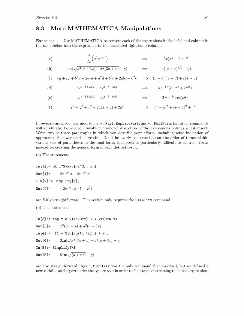
Exercise 8.3 89
8.3 More MATHEMATICA Manipulations
Exercise: Use MATHEMATICA to convert each of the expressions in the left-hand column inthe table below into the expression in the associated right-hand column:
(a)d
dx
(x2e−x
2)
=⇒ −2x(x2 − 1)e−x2
(b) sin(√a2(a+ 3x) + x2(3a+ x) + y) =⇒ sin((a+ x)3/2 + y)
(c) cg + cf + b2d+ 2abd+ a2d+ b2c+ 2abc+ a2c =⇒ (a+ b)2(c+ d) + c(f + g)
(d) a e(−b+iω)t + a e(−b−iω)t =⇒ a e−bt (e−iωt + eiωt)
(e) a e(−b+iω)t + a e(−b−iω)t =⇒ 2 a e−bt cos(ωt)
(f) x2 + y2 + z2 − 2a(x+ y) + 2a2 =⇒ (x− a)2 + (y − a)2 + z2
In several cases, you may need to invoke Part, ReplacePart, and/or FullForm, but other commandswill surely also be needed. Invoke microscopic dissection of the expressions only as a last resort.Write two or three paragraphs in which you describe your efforts, including some indication ofapproaches that were not successful. Don’t be overly concerned about the order of terms withinvarious sets of parentheses in the final form; that order is particularly difficult to control. Focusinstead on creating the general form of each desired result.
(a) The statements
In[1]:= D[ x^2*Exp[-x^2], x ]
Out[1]= 2e−x2
x− 2e−x2
x3
>In[2]:= Simplify[%];
Out[2]= −2e−x2
x(−1 + x2)
are fairly straightforward. This section only requires the Simplify command.
(b) The statements
In[3]:= tmp = a^2*(a+3*x) + x^2*(3*a+x)
Out[3]= x2(3a+ x) + a2(a+ 3x)
In[4]:= f1 = Sin[Sqrt[ tmp ] + y ]
Out[4]= Sin[√x2(3a+ x) + a2(a+ 3x) + y]
In[5]:= Simplify[%]
Out[5]= Sin(√
(a+ x)3 + y)
are also straightforward. Again, Simplify was the only command that was used, but we defined anew variable as the part under the square root in order to facilitate constructing the initial expression.
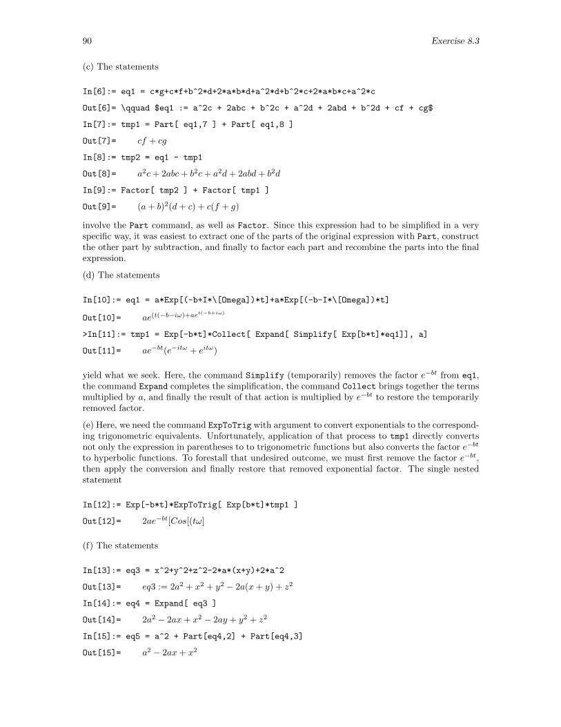
90 Exercise 8.3
(c) The statements
In[6]:= eq1 = c*g+c*f+b^2*d+2*a*b*d+a^2*d+b^2*c+2*a*b*c+a^2*c
Out[6]= \qquad $eq1 := a^2c + 2abc + b^2c + a^2d + 2abd + b^2d + cf + cg$
In[7]:= tmp1 = Part[ eq1,7 ] + Part[ eq1,8 ]
Out[7]= cf + cg
In[8]:= tmp2 = eq1 - tmp1
Out[8]= a2c+ 2abc+ b2c+ a2d+ 2abd+ b2d
In[9]:= Factor[ tmp2 ] + Factor[ tmp1 ]
Out[9]= (a+ b)2(d+ c) + c(f + g)
involve the Part command, as well as Factor. Since this expression had to be simplified in a veryspecific way, it was easiest to extract one of the parts of the original expression with Part, constructthe other part by subtraction, and finally to factor each part and recombine the parts into the finalexpression.
(d) The statements
In[10]:= eq1 = a*Exp[(-b+I*\[Omega])*t]+a*Exp[(-b-I*\[Omega])*t]
Out[10]= ae(t(−b−iω)+aet(−b+iω)
>In[11]:= tmp1 = Exp[-b*t]*Collect[ Expand[ Simplify[ Exp[b*t]*eq1]], a]
Out[11]= ae−bt(e−itω + eitω)
yield what we seek. Here, the command Simplify (temporarily) removes the factor e−bt from eq1,the command Expand completes the simplification, the command Collect brings together the termsmultiplied by a, and finally the result of that action is multiplied by e−bt to restore the temporarilyremoved factor.
(e) Here, we need the command ExpToTrig with argument to convert exponentials to the correspond-ing trigonometric equivalents. Unfortunately, application of that process to tmp1 directly convertsnot only the expression in parentheses to to trigonometric functions but also converts the factor e−bt
to hyperbolic functions. To forestall that undesired outcome, we must first remove the factor e−bt,then apply the conversion and finally restore that removed exponential factor. The single nestedstatement
In[12]:= Exp[-b*t]*ExpToTrig[ Exp[b*t]*tmp1 ]
Out[12]= 2ae−bt[Cos[(tω]
(f) The statements
In[13]:= eq3 = x^2+y^2+z^2-2*a*(x+y)+2*a^2
Out[13]= eq3 := 2a2 + x2 + y2 − 2a(x+ y) + z2
In[14]:= eq4 = Expand[ eq3 ]
Out[14]= 2a2 − 2ax+ x2 − 2ay + y2 + z2
In[15]:= eq5 = a^2 + Part[eq4,2] + Part[eq4,3]
Out[15]= a2 − 2ax+ x2
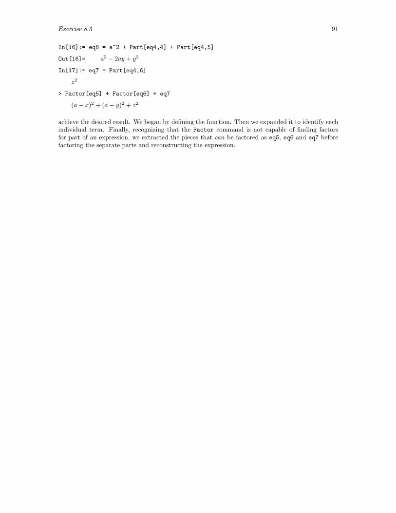
Exercise 8.3 91
In[16]:= eq6 = a^2 + Part[eq4,4] + Part[eq4,5]
Out[16]= a2 − 2ay + y2
In[17]:= eq7 = Part[eq4,6]
z2
> Factor[eq5] + Factor[eq6] + eq7
(a− x)2 + (a− y)2 + z2
achieve the desired result. We began by defining the function. Then we expanded it to identify eachindividual term. Finally, recognizing that the Factor command is not capable of finding factorsfor part of an expression, we extracted the pieces that can be factored as eq5, eq6 and eq7 beforefactoring the separate parts and reconstructing the expression.
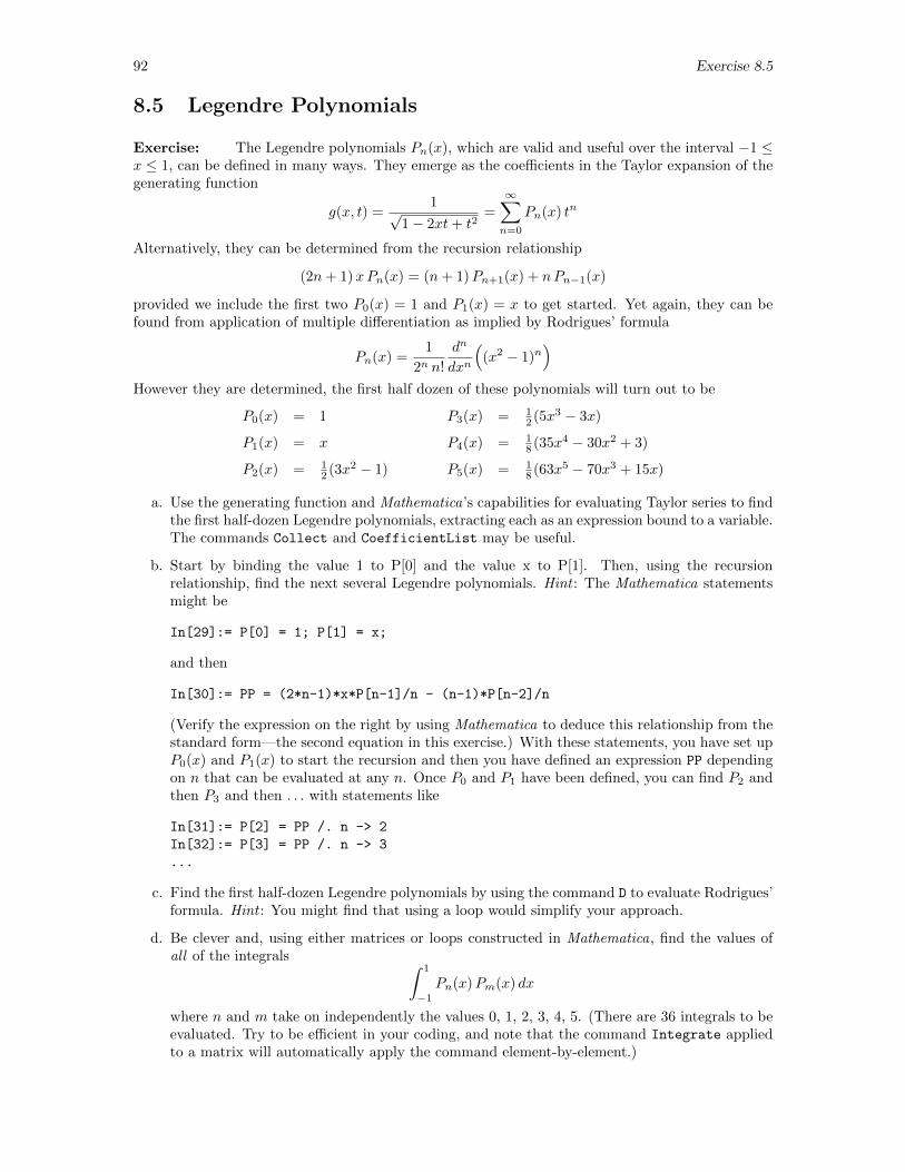
92 Exercise 8.5
8.5 Legendre Polynomials
Exercise: The Legendre polynomials Pn(x), which are valid and useful over the interval −1 ≤x ≤ 1, can be defined in many ways. They emerge as the coefficients in the Taylor expansion of thegenerating function
g(x, t) =1√
1− 2xt+ t2=
∞∑n=0
Pn(x) tn
Alternatively, they can be determined from the recursion relationship
(2n+ 1)xPn(x) = (n+ 1)Pn+1(x) + nPn−1(x)
provided we include the first two P0(x) = 1 and P1(x) = x to get started. Yet again, they can befound from application of multiple differentiation as implied by Rodrigues’ formula
Pn(x) =1
2n n!
dn
dxn
((x2 − 1)n
)However they are determined, the first half dozen of these polynomials will turn out to be
P0(x) = 1 P3(x) = 12 (5x3 − 3x)
P1(x) = x P4(x) = 18 (35x4 − 30x2 + 3)
P2(x) = 12 (3x2 − 1) P5(x) = 1
8 (63x5 − 70x3 + 15x)
a. Use the generating function and Mathematica’s capabilities for evaluating Taylor series to findthe first half-dozen Legendre polynomials, extracting each as an expression bound to a variable.The commands Collect and CoefficientList may be useful.
b. Start by binding the value 1 to P[0] and the value x to P[1]. Then, using the recursionrelationship, find the next several Legendre polynomials. Hint : The Mathematica statementsmight be
In[29]:= P[0] = 1; P[1] = x;
and then
In[30]:= PP = (2*n-1)*x*P[n-1]/n - (n-1)*P[n-2]/n
(Verify the expression on the right by using Mathematica to deduce this relationship from thestandard form—the second equation in this exercise.) With these statements, you have set upP0(x) and P1(x) to start the recursion and then you have defined an expression PP dependingon n that can be evaluated at any n. Once P0 and P1 have been defined, you can find P2 andthen P3 and then . . . with statements like
In[31]:= P[2] = PP /. n -> 2
In[32]:= P[3] = PP /. n -> 3
...
c. Find the first half-dozen Legendre polynomials by using the command D to evaluate Rodrigues’formula. Hint : You might find that using a loop would simplify your approach.
d. Be clever and, using either matrices or loops constructed in Mathematica, find the values ofall of the integrals ∫ 1
−1
Pn(x)Pm(x) dx
where n and m take on independently the values 0, 1, 2, 3, 4, 5. (There are 36 integrals to beevaluated. Try to be efficient in your coding, and note that the command Integrate appliedto a matrix will automatically apply the command element-by-element.)
Exercise 8.5 93
e. Within Mathematica, obtain graphs of the first six Legendre polynomials over the interval−1 ≤ x ≤ 1.
f. It is known that a function f(x) defined over the interval −1 ≤ x ≤ 1 can be expanded in aseries of Legendre polynomials of the form f(x) =
∑an Pn(x) where the coefficients an are
given by
an =2n+ 1
2
∫ 1
−1
f(x)Pn(x) dx
Find the first six coefficients for the expansion of the function f(x) = 0 when −1 < x < 0 andf(x) = 1 when 0 < x < 1. Then, construct the (partial) series representing this function andobtain a graph of that approximation to compare with the graph of the original function.
g. Mathematica actually knows quite a bit about many of the important special functions ofmathematical physics. In particular, the the n-th Legendre polynomial as a function of x isknown by the name LegendreP[n, x] and is described fully in the Mathematica manuals.Take a look at that documentation and then use that function to determine the first severalLegendre polynomials.
Solution: (a) One quick way to find the Legendre polynomials is through the Taylor expansionof the generating function,
g(x, t) =1√
1− 2xt+ t2=
∞∑n=0
Pn(x) tn
The Legendre polynomials are the coefficients in this expansion. To find these coefficients usingMathematica, we first define the generating function with the statement
In[1]:= g = 1/Sqrt[1 - 2*x*t + t^2]
Out[1]=1√
1 + t2 − 2tx
Next, we create the first six terms in the Taylor series expansion of the generating function. Toaccomplish this task we execute the statements
In[2]:= Taylorser = Series[ %, t, 0, 6 ];
In[3]:= Simplify[%]
Out[3]= 1 + x t+
(−1 + 3x2
)t2
2+x(−3 + 5x2
)t3
2+
(3− 30x2 + 35x4
)t4
8+
x(15− 70x2 + 63x4
)t5
8+
(−5 + 105x2 − 315x4 + 231x6
)t6
16+O[t]
7
Within the second argument to the Series function, the first argument, t, identifies the variable tobe expanded around, the second argument, 0, identifies the point to expand about, and the thirdargument tells Mathematica how far to carry the expansion (to the sixth power).
After simplifying the expansion, we convert the series into a polynomial with the statement
In[4]:= poly = Normal[%]
Out[4]= 1 + t x+t2(−1 + 3x2
)2
+t3 x
(−3 + 5x2
)2
+t4(3− 30x2 + 35x4
)8
+
94 Exercise 8.5
t5 x(15− 70x2 + 63x4
)8
+t6(−5 + 105x2 − 315x4 + 231x6
)16
To further simplify the solution, we expand and then collect the terms in the polynomial. Weaccomplish this task by executing the statements
In[5]:= Expand[poly];
In[6]:= poly2 = Collect[%, t]
Out[6]= 1 + t x+ t2(−1
2+
3x2
2
)+ t3
(−3x
2+
5x3
2
)+ t4
(3
8− 15x2
4+
35x4
8
)+
t5(
15x
8− 35x3
4+
63x5
8
)+ t6
(− 5
16+
105x2
16− 315x4
16+
231x6
16
)The second argument to the Collect function indicates the variable whose powers are to be sortedout. Now, we extract the coefficients from the polynomial and place them in a list. To accomplishthis task, we use the CoefficientList function and execute the statement
In[7]:= list1 = CoefficientList[ poly2, t ]
Out[7]=
1, x,−1
2+
3x2
2,−3x
2+
5x3
2,
3
8− 15x2
4+
35x4
8,
15x
8− 35x3
4+
63x5
8,
− 5
16+
105x2
16− 315x4
16+
231x6
16
The second argument to the CoefficientList function tells Mathematica to list the coefficientsfor the different powers of the variable t, starting at t0. Once we have this list, we can find aparticular Legendre polynomial by accessing an element in the list. For example, to find the Legendrepolynomial P2(x) we execute the statement
In[8]:= P[2] = list1[[3]]
Out[8]= −1
2+
3x2
2
(b) Another way to find the Legendre polynomials is by using the recursion relationship
(2n+ 1)xPn(x) = (n+ 1)Pn+1(x) + nPn−1(x)
First, we must recast this relationship as an expression giving a particular Legendre polynomial interms of the previous two, i.e., in an expression of the form
Pn(x) = APn−1(x) +B Pn−2(x)
where A and B potentially depend on n and x but not on the Legendre polynomials.
The statement in the exercise contends that the expression
Pn(x) =(2n− 1)xPn−1(x)
n− (n− 1)Pn−2(x)
n
is a rewriting of the recursion relationship. We now prove this relationship. Accepting the initialrecursion relationship, we first translate the indices so that the Legendre polynomial with the highestindex is labeled Pn and then solve that result for Pn. We start by executing the statement
In[9]:= r = (2*n + 1)*x*P[n] == (n + 1)* P[n+1] + n*P[n-1];
Exercise 8.5 95
which sets up the initial recursion relationship. Now we substitute n− 1 for n and then solve for Pnby executing the statements
In[10]:= s = r/. n -> n - 1;
In[11]:= r = Solve[ s, P[ n] ]
Out[11]=
Pn → −
((−1 + n) P−2+n − (1 + 2 (−1 + n)) xP−1+n
n
)We then expand and simplify the result to see that it is indeed the result given in part (b) with thestatements
In[12]:= ExpandAll[r]
Out[12]=
Pn → −P−2+n +
P−2+n
n+ 2xP−1+n −
xP−1+n
n
In[13]:= Simplify[%]
Out[13]=
Pn →
− (−1 + n) P−2+n + (−1 + 2n) xP−1+n
n
This is indeed the result given in part (b). Now, if we fix the first two Legendre polynomials, we canuse this recursion relationship to obtain all subsequent polynomials in turn. To fix the polynomialswe write the statement
In[14]:= P[0] = 1; P[1] = x;
Now we enter the suggested expression with the statement
In[15]:= PP = (2*n-1)*x*P[n-1]/n - (n-1)*P[n-2]/n
Out[15]=− (−1 + n) P−2+n
n+
(−1 + 2n) xP−1+n
n
At last we can find the Legendre polynomials. For example we can find the Legendre polynomialP2(x) with the substitution
In[16]:= P[2] = PP /. n -> 2
Out[16]=−1
2+
3x2
2
We can find all Legendre polynomials by making similar substitutions ( i.e. n = 3 for P3(x) and soon).
(c) The Legendre polynomials can also be defined with Rodrigues’ formula. First, we enter Ro-drigues’ formula using the D function with the statement
In[17]:= Rod = 1/(2^n * n!)*D[(x^2 - 1)^n, x, n];
The second argument of this function contains the variable, x, with respect to which the derivativeis taken and the number of times, n, that the differentiation is carried out. Now, we can find theLegendre polynomials by substituting different values of n into Rod. The statement to effect thisaction is
In[18]:= P[0] = Simplify[ Rod /. n -> 0 ]
96 Exercise 8.5
Out[18]= 1
We repeat this command to obtain the first six Legendre polynomials by executing the statements
In[19]:= P[1] = Simplify[ Rod /. n -> 1 ];
In[20]:= P[2] = Simplify[ Rod /. n -> 2 ];
In[21]:= P[3] = Simplify[ Rod /. n -> 3 ];
In[22]:= P[4] = Simplify[ Rod /. n -> 4 ];
In[23]:= P[5] = Simplify[ Rod /. n -> 5 ];
(d) To evaluate the requested integrals (and demonstrate the orthogonality of the Legendre polyno-mials with weight 1 on the interval −1 ≤ x ≤ 1), we could create a matrix containing the variousintegrands and then use the function Integrate to integrate each element in that matrix. Atfirst, the task may look daunting. Luckily, Mathematica provides straightforward tools to deal withthis problem. We begin by creating a list of values for the first six Legendre polynomials as weredetermined in (a), (b), and (c).
We use the values for P[n] found in part (c) to create the matrix of products of P [n]P [m]. Notethat we must use P[n-1] and let n got to six when creating the table because tables in Mathematicareference their first element as one and not zero. To create the table we write the statement
In[24]:= Table[ P[n - 1]*P[m - 1], n, 6, m, 6 ];
We now use the Integrate function to integrate every element in the matrix with the statement
In[25]:= Integrate[ %, x, -1, 1 ]
Out[25]=
2, 0, 0, 0, 0, 0, 0, 2
3, 0, 0, 0, 0, 0, 0, 2
5, 0, 0, 0, 0, 0, 0, 2
7, 0, 0,
0, 0, 0, 0, 2
9, 0, 0, 0, 0, 0, 0, 2
11
In[26]:= MatrixForm[%]
Out[26]//MatrixForm=
2 0 0 0 0 00 2/3 0 0 0 00 0 2/5 0 0 00 0 0 2/7 0 00 0 0 0 2/9 00 0 0 0 0 2/11
Evidently, these integrals are 0 for all values of n and m except when n = m. Further, when n = m,it appears as if the value of the integral is 2/(2n+ 1). Thus, we apparently can infer that∫ 1
−1
Pn(x)Pm(x) dx =2
2n+ 1δnm
(Here, δnm, the Kronecker delta, is 0 when n 6= m and 1 when n = m.) This result is correct ingeneral, though our evidence supports its correctness only when n,m ≤ 5.
We can understand some of the zeroes in the above matrix by noting the parity of the Legendrepolynomials: those for even n are even functions of x, those for odd n are odd functions of x. Thus,whenever we integrate a product of two polynomials, one of which is even and the other of which isodd, on symmetric limits, the integral (which is then an integral of an odd function on symmetric
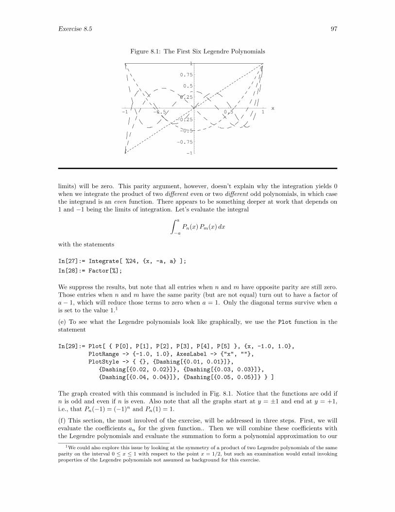
Exercise 8.5 97
Figure 8.1: The First Six Legendre Polynomials
-1 -0.5 0.5 1x
-1
-0.75
-0.5
-0.25
0.25
0.5
0.75
1
limits) will be zero. This parity argument, however, doesn’t explain why the integration yields 0when we integrate the product of two different even or two different odd polynomials, in which casethe integrand is an even function. There appears to be something deeper at work that depends on1 and −1 being the limits of integration. Let’s evaluate the integral∫ a
−aPn(x)Pm(x) dx
with the statements
In[27]:= Integrate[ %24, x, -a, a ];
In[28]:= Factor[%];
We suppress the results, but note that all entries when n and m have opposite parity are still zero.Those entries when n and m have the same parity (but are not equal) turn out to have a factor ofa − 1, which will reduce those terms to zero when a = 1. Only the diagonal terms survive when ais set to the value 1.1
(e) To see what the Legendre polynomials look like graphically, we use the Plot function in thestatement
In[29]:= Plot[ P[0], P[1], P[2], P[3], P[4], P[5] , x, -1.0, 1.0,
PlotRange -> -1.0, 1.0, AxesLabel -> "x", "",
PlotStyle -> , Dashing[0.01, 0.01],
Dashing[0.02, 0.02], Dashing[0.03, 0.03],
Dashing[0.04, 0.04], Dashing[0.05, 0.05] ]
The graph created with this command is included in Fig. 8.1. Notice that the functions are odd ifn is odd and even if n is even. Also note that all the graphs start at y = ±1 and end at y = +1,i.e., that Pn(−1) = (−1)n and Pn(1) = 1.
(f) This section, the most involved of the exercise, will be addressed in three steps. First, we willevaluate the coefficients an for the given function.. Then we will combine these coefficients withthe Legendre polynomials and evaluate the summation to form a polynomial approximation to our
1We could also explore this issue by looking at the symmetry of a product of two Legendre polynomials of the sameparity on the interval 0 ≤ x ≤ 1 with respect to the point x = 1/2, but such an examination would entail invokingproperties of the Legendre polynomials not assumed as background for this exercise.
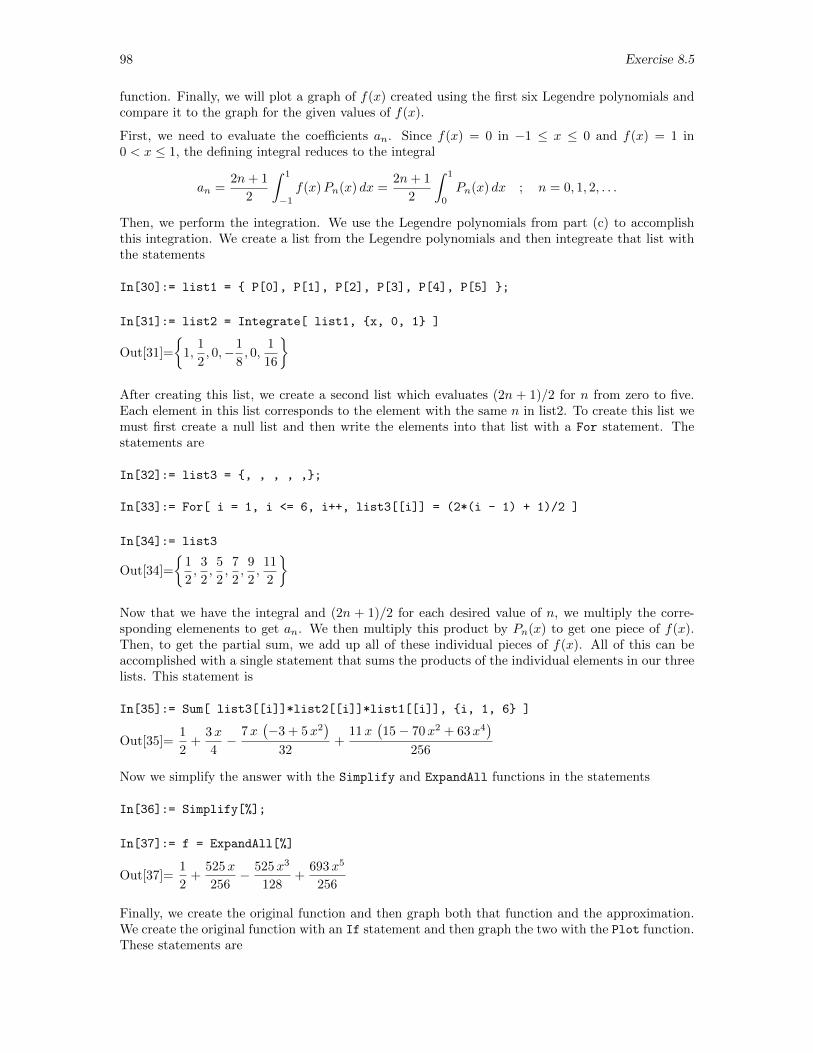
98 Exercise 8.5
function. Finally, we will plot a graph of f(x) created using the first six Legendre polynomials andcompare it to the graph for the given values of f(x).
First, we need to evaluate the coefficients an. Since f(x) = 0 in −1 ≤ x ≤ 0 and f(x) = 1 in0 < x ≤ 1, the defining integral reduces to the integral
an =2n+ 1
2
∫ 1
−1
f(x)Pn(x) dx =2n+ 1
2
∫ 1
0
Pn(x) dx ; n = 0, 1, 2, . . .
Then, we perform the integration. We use the Legendre polynomials from part (c) to accomplishthis integration. We create a list from the Legendre polynomials and then integreate that list withthe statements
In[30]:= list1 = P[0], P[1], P[2], P[3], P[4], P[5] ;
In[31]:= list2 = Integrate[ list1, x, 0, 1 ]
Out[31]=
1,
1
2, 0,−1
8, 0,
1
16
After creating this list, we create a second list which evaluates (2n + 1)/2 for n from zero to five.Each element in this list corresponds to the element with the same n in list2. To create this list wemust first create a null list and then write the elements into that list with a For statement. Thestatements are
In[32]:= list3 = , , , , ,;
In[33]:= For[ i = 1, i <= 6, i++, list3[[i]] = (2*(i - 1) + 1)/2 ]
In[34]:= list3
Out[34]=
1
2,
3
2,
5
2,
7
2,
9
2,
11
2
Now that we have the integral and (2n + 1)/2 for each desired value of n, we multiply the corre-sponding elemenents to get an. We then multiply this product by Pn(x) to get one piece of f(x).Then, to get the partial sum, we add up all of these individual pieces of f(x). All of this can beaccomplished with a single statement that sums the products of the individual elements in our threelists. This statement is
In[35]:= Sum[ list3[[i]]*list2[[i]]*list1[[i]], i, 1, 6 ]
Out[35]=1
2+
3x
4−
7x(−3 + 5x2
)32
+11x
(15− 70x2 + 63x4
)256
Now we simplify the answer with the Simplify and ExpandAll functions in the statements
In[36]:= Simplify[%];
In[37]:= f = ExpandAll[%]
Out[37]=1
2+
525x
256− 525x3
128+
693x5
256
Finally, we create the original function and then graph both that function and the approximation.We create the original function with an If statement and then graph the two with the Plot function.These statements are
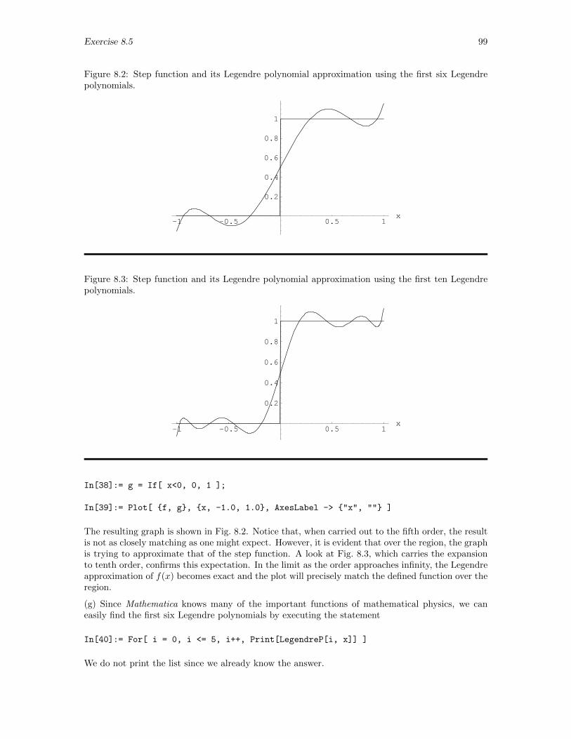
Exercise 8.5 99
Figure 8.2: Step function and its Legendre polynomial approximation using the first six Legendrepolynomials.
-1 -0.5 0.5 1x
0.2
0.4
0.6
0.8
1
Figure 8.3: Step function and its Legendre polynomial approximation using the first ten Legendrepolynomials.
-1 -0.5 0.5 1x
0.2
0.4
0.6
0.8
1
In[38]:= g = If[ x<0, 0, 1 ];
In[39]:= Plot[ f, g, x, -1.0, 1.0, AxesLabel -> "x", "" ]
The resulting graph is shown in Fig. 8.2. Notice that, when carried out to the fifth order, the resultis not as closely matching as one might expect. However, it is evident that over the region, the graphis trying to approximate that of the step function. A look at Fig. 8.3, which carries the expansionto tenth order, confirms this expectation. In the limit as the order approaches infinity, the Legendreapproximation of f(x) becomes exact and the plot will precisely match the defined function over theregion.
(g) Since Mathematica knows many of the important functions of mathematical physics, we caneasily find the first six Legendre polynomials by executing the statement
In[40]:= For[ i = 0, i <= 5, i++, Print[LegendreP[i, x]] ]
We do not print the list since we already know the answer.
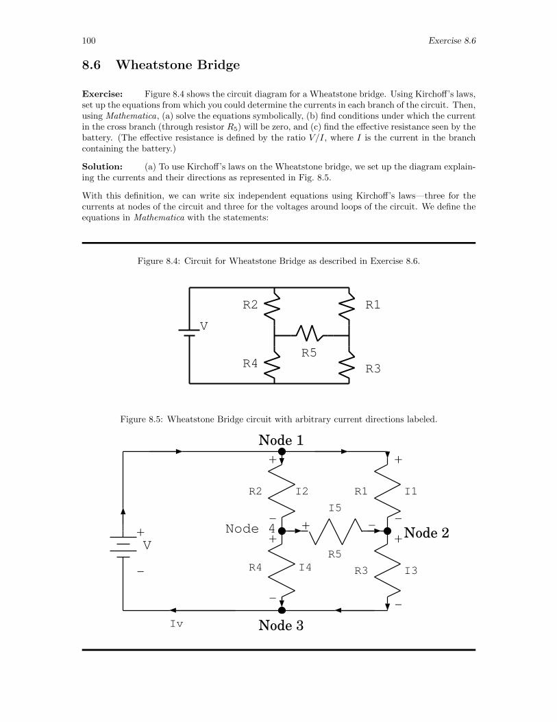
100 Exercise 8.6
8.6 Wheatstone Bridge
Exercise: Figure 8.4 shows the circuit diagram for a Wheatstone bridge. Using Kirchoff’s laws,set up the equations from which you could determine the currents in each branch of the circuit. Then,using Mathematica, (a) solve the equations symbolically, (b) find conditions under which the currentin the cross branch (through resistor R5) will be zero, and (c) find the effective resistance seen by thebattery. (The effective resistance is defined by the ratio V/I, where I is the current in the branchcontaining the battery.)
Solution: (a) To use Kirchoff’s laws on the Wheatstone bridge, we set up the diagram explain-ing the currents and their directions as represented in Fig. 8.5.
With this definition, we can write six independent equations using Kirchoff’s laws—three for thecurrents at nodes of the circuit and three for the voltages around loops of the circuit. We define theequations in Mathematica with the statements:
Figure 8.4: Circuit for Wheatstone Bridge as described in Exercise 8.6.
V
R1R2
R3R4R5
Figure 8.5: Wheatstone Bridge circuit with arbitrary current directions labeled.
R5R4
R2
R3
R1
V
I1
I3I4
I2
I5
Iv
-
+ +
-
+
++
+
- -
-
-
Node 1
Node 2
Node 3
Node 4
Exercise 8.6 101
In[1]:= IEqn1 = Iv - I2 - I1 == 0;
In[2]:= IEqn2 = I1 + I5 - I3 == 0;
In[3]:= IEqn3 = I3 + I4 - Iv == 0;
In[4]:= VolEqn1 = V - I1*R1 - I3*R3 == 0;
In[5]:= VolEqn2 = V - I2*R2 - I4*R4 == 0;
In[6]:= VolEqn3 = V - I2*R2 - I5*R5 -
I3*R3 == 0;
Set net current into Node 1 = 0.Set net current into Node 2 = 0.Set net current into Node 3 = 0.Set voltage drop clockwise around loop con-taining V , R1, and R3 = 0.Set voltage drop clockwise around loop con-taining V , R2, and R4 = 0.Set voltage drop clockwise around loop con-taining V , R2, R5, and R3 = 0.
We solve these (linear) equations for the unknown currents with the statement
In[7]:= soln = Simplify[ Solve[ IEqn1, IEqn2, IEqn3, VolEqn1, VolEqn2, VolEqn3,
I1, I2, I3, I4, I5, Iv ] ]
Out[7]=
I5 →
− (R2R3V ) +R1R4V
R3 (R4R5 +R2 (R4 +R5)) +R1 (R4 (R3 +R5) +R2 (R3 +R4 +R5)),
I4 →(R3 (R2 +R5) +R1 (R3 +R5))V
R3 (R4R5 +R2 (R4 +R5)) +R1 (R4 (R3 +R5) +R2 (R3 +R4 +R5)),
Iv →((R3 +R4)R5 +R1 (R3 +R4 +R5) +R2 (R3 +R4 +R5))V
R3 (R4R5 +R2 (R4 +R5)) +R1 (R4 (R3 +R5) +R2 (R3 +R4 +R5)),
I2 →(R3R5 +R1 (R3 +R4 +R5))V
R3 (R4R5 +R2 (R4 +R5)) +R1 (R4 (R3 +R5) +R2 (R3 +R4 +R5)),
I1 →(R4R5 +R2 (R3 +R4 +R5))V
R3 (R4R5 +R2 (R4 +R5)) +R1 (R4 (R3 +R5) +R2 (R3 +R4 +R5)),
I3 →(R1R4 +R4R5 +R2 (R4 +R5))V
R3 (R4R5 +R2 (R4 +R5)) +R1 (R4 (R3 +R5) +R2 (R3 +R4 +R5))
Here, the function Solve solves a system of linear equations for unknowns as long as the num-ber of unknowns is equal to or less than the number of equations (and the equations are linearlyindependent). Note that, in Mathematica’s solution, the currents all share the same denominator.
(b) In particular, we can readily see from the solution for I5 that, if R3R2 = R4R1, the current I5will be zero. Using Mathematica explicitly, we can find the condition under which I5 will be zerowith the statement2
In[8]:= cond = Solve[ Numerator[ soln[[1]][[1]][[2]]] == 0, R1 ]
Out[8]=
R1 →
R2R3
R4
We see that as long as R1 is equal to R2R3/R4 there will be no current through the bridge and weare free to choose R5 to be anything without affecting the circuit. This relationship provides thebasis for the primary use of the Wheatstone bridge. Suppose R1 is an unknown resistor and R2, R3,and R4 can be adjusted. Suppose, further, that a galvanometer is placed in series with R5. Then,by adjusting R2, R3, and R4, we can balance the bridge so that the galvanometer shows no current.Finally, we can use the balance condition here deduced to calculate the value of R1 from the known
2Note that the order in which Mathematica presents you with the solutions for the six unknown currents maydiffer from the order above. You must therefore be sure to replace the numbers identifying parts of the solution withvalues appropriate to your solution.
102 Exercise 8.6
values of R2, R3, and R4. Before the days of high-quality ohmmeters, the Wheatstone bridge wasan essential piece of laboratory equipment.
(c) Finally, to find the effective resistance, we divide the current Iv passing through the branch withthe battery by the voltage V of the battery. Since we have already solved for Iv the task involvesthe single statement
In[9]:= effre = V / soln[[1]][[3]][[2]]
Out[9]=R3 (R4R5 +R2 (R4 +R5)) +R1 (R4 (R3 +R5) +R2 (R3 +R4 +R5))
(R3 +R4)R5 +R1 (R3 +R4 +R5) +R2 (R3 +R4 +R5)
It turns out that if we choose R1 = R2 = R3 = R4, the effective resistance will be R1. Further,if this is done, note that R1 = R2R3/R4 and, therefore, we are free to choose R5. These two itemsare confirmed in Mathematica through substitution. A sample of this confirmation might includethe Mathematica statements
In[10]:= effre /. R1-> 2*R, R2-> 2*R, R3-> 2*R, R4->2*R, R5->2*R
Out[10]= 2R
In[11]:= effre /. R1-> 2*R, R2-> 2*R, R3-> 2*R, R4->2*R, R5->33*R
Out[11]= 2R
Changing R5 here does not change the effective resistance seen by the battery. More generally, wecould simply set R2, R3, and R4 equal to R1 with the statement
In[12]:= Simplify[ effre /. R2 -> R1, R3 -> R1, R4 -> R ]
Out[12]= R1
to confirm that the effective resistance when all four resistors R1, R2, R3, and R4 are the same is,in fact, equal to any one of those resistors and that it does not depend in any way on the value ofR5.
Exercise 8.7 103
8.7 Quantum Wave Scattering
Exercise: In the scattering of a quantum wave from a rectangular barrier in particular circum-stances, we find that the wave function must be expressed in three pieces in the form
ψ(x) = Aeikx +Be−ikx x < 0
= D cosh(κx) + F sinh(κx) 0 < x < w
= Ceikx x > w
where k and κ are constants related to the energy of the particle and the height of the barrier,A is a constant reflecting the intensity of the incident beam, and B, D, F , and C are constantsto be determined by imposing the requirement that the wave function and its first derivative becontinuous both at x = 0 and at x = w, i.e., that
ψ(0−) = ψ(0+) ; ψ(w−) = ψ(w+) ;dψ
dx
∣∣∣∣0−
=dψ
dx
∣∣∣∣0+
;dψ
dx
∣∣∣∣w−
=dψ
dx
∣∣∣∣w+
where superscript plus and minus signs identify points slightly below and slightly above the indicatedvalue of x, respectively. (While k and κ can be taken to be real for this barrier, the constants A,B, C, D, and F may—and probably will—be complex.) Use Mathematica’s abilities to manipulateexpressions to
(a) Obtain the equations determining B, C, D, and F by imposing the stated boundary conditionson these solutions.
(b) Solve those equations for those constants (expressing each as a multiple of the constant A).(c) Show that the reflection and transmission coefficients R and T defined by R = |B/A|2 and
T = |C/A|2 are given by
R =
∣∣∣∣BA∣∣∣∣2 =
(κ2 + k2)2 sinh2 κw
4κ2k2 + (κ2 + k2)2 sinh2 κw; T =
∣∣∣∣CA∣∣∣∣2 =
4k2κ2
4κ2k2 + (κ2 + k2)2 sinh2 κw
Here, the vertical bars symbolize the absolute value of the complex number enclosed by them.(d) Verify that R+ T = 1.
Solution: (a) In the scattering of a quantum wave from a rectangular barrier, the wave functionis defined in three equations. One of these equations describes the wave on the side coming into thebarrier, another the wave within the barrier, and the third the wave as it emerges from the barrier.For this problem, we begin by defining the three equations in Mathematica with the statements
In[1]:= \[Psi]1 = A*Exp[I*k*x]+B*Exp[-I*k*x];
In[2]:= \[Psi]2 = D*Cosh[\[Kappa]*x] +
F*Sinh[\[Kappa]*x];
In[3]:= \[Psi]3 = C*Exp[I*k*x];
Define the three wave functions, suppress-ing output.
(Recall that, within Mathematica, the variable I is equivalent to√−1.) Now, preparing to impose
the boundary conditions, we evaluate the derivatives of these functions with the statements
In[4]:= diff1 = D[ \[Psi]1, x ];
In[5]:= diff2 = D[ \[Psi]2, x ];
In[6]:= diff2 = D[ \[Psi]3, x ];
Evaluate the derivatives of Ψ1, Ψ2, and Ψ3
with respect to x, again suppressing output.
Physically, the wave function and its first derivative must be continuous at all points. In particular,at the points of discontinuity in the potential, i.e., at x = 0 and x = w, both the wave functions andtheir derivatives on either side of the boundary should be equivalent. Thus, we must require thatthe wave functions and their derivatives satisfy the four equations obtained with the statements
104 Exercise 8.7
In[7]:= eq1 = \[Psi]1==\[Psi]2/.x->0
Out[7]= A+B = DIn[8]:= eq2 = \[Psi]2==\[Psi]3/.x->w
eval(Psi2,x=w) = eval(Psi3,x=w);
Out[8]= D cosh(w κ) + F sinh(w κ) = C ei k w
In[9]:= eq3 = diff1==diff2/x->0
Out[9]= iAk − iB k = F κIn[10]:= eq4 = eq4 = diff2 == diff3 /. x -> w
Out[10]=F κ cosh(w κ) +Dκ sinh(w κ) = iC ei k w k
Establish the four equations expressing therequired boundary conditions.
(b) We can now solve these four equations for the four coefficients B, C, D, and F by executing thestatement
In[11]:= soln = Solve[ eq1,eq2,eq3,eq4, B,C,D,F ];
Out[11]= C → messC , D → messD, B → messB , F → messF
where the several messes are quite complicated—They are recorded in full detail in the appendixat the end of this solution.—but their details are not here particularly important, suffice it to notethat each one has an overall factor of A.
(c) While these solutions have been quickly obtained, they are not the quantities of primary interest.From here, our task is to find the transmission and reflection coefficients and beat them into theform given in the statement of the exercise. Since the reflection and transmission coefficients aredetermined by B and C, respectively, we shall in what follows ignore D and F . We begin byextracting B and C and evaluating the amplitudes for reflection r and transmission t with thestatements
In[12]:= eqb = Simplify[soln[[1]][[3]][[2]]];
In[13]:= r = eqb/A
Out[13]=
(k2 + κ2
)sinh(w κ)
2 i k κ cosh(w κ) + (k2 − κ2) sinh(w κ)
In[14]:= eqc = Simplify[ExpToTrig[soln[[1]][[1]][[2]]]];
In[15]:= t = eqc/A
Out[15]=2 k κ (i cos(k w) + sin(k w))
2 i k κ cosh(w κ) + (k2 − κ2) sinh(w κ)
We are, of course, not interested in r and t but rather in R = |r|2 and T = |t|2. We can move inthat direction by finding the absolute value of r and t. Since the Mathematica object Abs[] is onlyevaluated for numeric quantities, we will transform r and t into the form a + ib and then evaluatethe absolute value using
√a2 + b2 with the statements
In[16]:= rbottom = 1/r[[3]];
In[17]:= rtop = r[[1]]*r[[2]];
In[18]:= imrtop = rtop*(rbottom[[1]]/I);
In[19]:= rertop = rtop*(-rbottom[[2]]);
In[20]:= ccrbot = rbottom[[1]] - rbottom[[2]];
In[21]:= rbot = Simplify[rbottom*ccrbot];
In[22]:= realr = rertop/rbot;
In[23]:= imr = imrtop/rbot;
In[24]:= absr = Simplify[Sqrt[realr^2+imr^2]];
In[25]:= R = absr^2;
Start with the form a/(bi+ c).
Multiply by (bi− c)/(bi− c).
Then break it into the real and imaginarypieces.
Exercise 8.7 105
In[26]:= R = Simplify[R /. Cosh[2 w \[Kappa]]
-> (2*(Sinh[w*\[Kappa]])^2 + 1)];
Out[26]=
(k2 + κ2
)2sinh(w κ)
2
4 k2 κ2 + (k2 + κ2)2
sinh(w κ)2
Substitute in the identity cosh 2x =2 sinh2 x+ 1
(Because the output produced by these statements is involved and not particularly illuminating, wesuppress it.) Then we do the same for t by invoking the statements
In[27]:= tbottom = 1/t[[5]];
In[28]:= ttop = Expand[t[[1]]*t[[2]]*
t[[3]]*t[[4]]];
In[29]:= cctbot = tbottom[[1]]-tbottom[[2]];
Break t into the real and imaginary pieces.
In[30]:= ttop2 = Expand[ttop*cctbot];
In[31]:= imttop = Simplify[Expand[(ttop2[[2]]
+ ttop2[[3]] + ttop2[[4]])/I]];
In[32]:= rettop = Simplify[ttop2[[1]] +
ttop2[[5]] + ttop2[[6]]];
In[33]:= tbot = Simplify[tbottom*cctbot];
In[34]:= realt = Simplify[rettop/tbot];
In[35]:= imt = Simplify[imttop/tbot];
In[36]:= abst = Simplify[Sqrt[realt^2 + imt^2]];
In[37]:= T = abst^2;
In[38]:= T = T /. Cosh[2 w \[Kappa]] ->
(2*(Sinh[w *\[Kappa]])^2 + 1);
In[39]:= T = Simplify[T]
Out[39]=4 k2 κ2
4 k2 κ2 + (k2 + κ2)2
sinh(w κ)2
Substitute in the identity cosh 2x =2 sinh2 x+ 1
At last (except for order of terms, about which we can really do nothing), we have the expressionsgiven in the exercise.
(d) Now that we have the simplified equations for R and T we want to confirm that the sum ofR+ T is indeed 1. The single statement
In[40]:= Simplify[R + T]
Out[40]= 1
confirms that R+ T = 1.
Appendix to Exercise 8.7
We record here the several messes that were represented by abbreviations in part (b) of thisexercise: messC →
−2Ak κ(
cosh(w κ)2 − sinh(w κ)
2)
ei k w (−2 k κ cosh(w κ) + i k2 sinh(w κ)− iκ2 sinh(w κ)),
messD →2(iAk κ cosh(w κ) +Ak2 sinh(w κ)
)2 i k κ cosh(w κ) + k2 sinh(w κ)− κ2 sinh(w κ)
,
messB → −
(−(Ak2 sinh(w κ)
)−Aκ2 sinh(w κ)
2 i k κ cosh(w κ) + k2 sinh(w κ)− κ2 sinh(w κ)
),
messF →−2
(Ak2 cosh(w κ) + iAk κ sinh(w κ)
)2 i k κ cosh(w κ) + k2 sinh(w κ)− κ2 sinh(w κ)
106 Exercise 8.8
8.8 Black Body Spectrum
Exercise: The distribution of wavelengths λ in the blackbody spectrum at (absolute) temper-ature T is given by
u(λ, T ) =8πch
λ5
1
ech/(λkT ) − 1
where c is the speed of light, h is Planck’s constant, and k is Boltzmann’s constant. In terms of thevariable y = ch/λkT , this function has the alternative expression
(ch)4 u(λ, T )
8π(kT )5= f(y) =
y5
ey − 1
(a) Verify this transformed form and then, using MATHEMATICA, (b) obtain a graph of f(y) versusy, making sure to extend the graph over an interval that includes its peak and estimate the value ofy at which that peak occurs; (c) show that the peak occurs for values of y satisfying
(y − 5) ey + 5 = 0
(d) obtain a graph of this function versus y; (e) make another estimate of the value of y at which theoriginal function has its maximum; and (f) show that the wavelength λm at which this maximumoccurs satisfies
λmT = 0.28978× 10⁻²m K
Hints: (1) Remember that maxima in a function occur where the derivative of that function withrespect to the appropriate variable is zero. (2) Because ey varies rapidly with y, you may have toplay a bit to find a suitable range of values of y over which to plot these graphs.
Solution: (a) To verify the dimensionless transformation, we enter the original equation withthe statement
In[1]:= u = (8*Pi*c*h/\[Lambda]^5)*(1/(Exp[c*h/(\[Lambda]*k*T)]-1))
Out[1]=8πch
(−1 + ech/kTλ)λ5
Then, we create the left hand side of the second equation above with the statement
In[2]:= tmp = (c*h)^4/(8*Pi*(k*T)^5)*u
Out[2]=c5h5
(−1 + ech/kTλ − 1)k5T 5λ5
and, finally, effect the last transformation with the statement
In[3]:= f = tmp /. h->(y*\[Lambda]*k*T)/c
Out[3]= y5
−1+ey
(b) We are then asked to graph f(y) versus y. The MATHEMATICA statement
\verb!In[4]:= plt = Plot[ f, y, 0.1, 20.0, PlotRange->0.0,25.0,
PlotStyle->Thickness[0.01],Black,
TicksStyle->Directive[12], AxesLabel->Style["y",Bold,20],Style["f",Bold,20]]
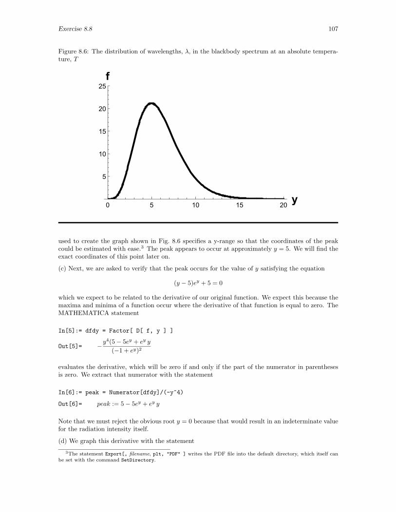
Exercise 8.8 107
Figure 8.6: The distribution of wavelengths, λ, in the blackbody spectrum at an absolute tempera-ture, T
0 5 10 15 20y
5
10
15
20
25f
used to create the graph shown in Fig. 8.6 specifies a y-range so that the coordinates of the peakcould be estimated with ease.3 The peak appears to occur at approximately y = 5. We will find theexact coordinates of this point later on.
(c) Next, we are asked to verify that the peak occurs for the value of y satisfying the equation
(y − 5)ey + 5 = 0
which we expect to be related to the derivative of our original function. We expect this because themaxima and minima of a function occur where the derivative of that function is equal to zero. TheMATHEMATICA statement
In[5]:= dfdy = Factor[ D[ f, y ] ]
Out[5]= −y4(5− 5ey + ey y
(−1 + ey)2
evaluates the derivative, which will be zero if and only if the part of the numerator in parenthesesis zero. We extract that numerator with the statement
In[6]:= peak = Numerator[dfdy]/(-y^4)
Out[6]= peak := 5− 5ey + ey y
Note that we must reject the obvious root y = 0 because that would result in an indeterminate valuefor the radiation intensity itself.
(d) We graph this derivative with the statement
3The statement Export[, filename, plt, "PDF" ] writes the PDF file into the default directory, which itself canbe set with the command SetDirectory.
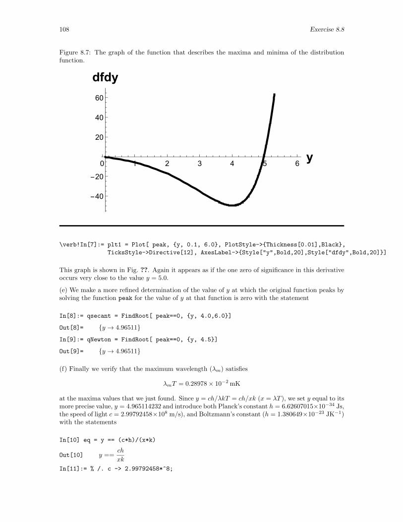
108 Exercise 8.8
Figure 8.7: The graph of the function that describes the maxima and minima of the distributionfunction.
0 1 2 3 4 5 6y
-40
-20
20
40
60
dfdy
\verb!In[7]:= plt1 = Plot[ peak, y, 0.1, 6.0, PlotStyle->Thickness[0.01],Black,
TicksStyle->Directive[12], AxesLabel->Style["y",Bold,20],Style["dfdy",Bold,20]]
This graph is shown in Fig. ??. Again it appears as if the one zero of significance in this derivativeoccurs very close to the value y = 5.0.
(e) We make a more refined determination of the value of y at which the original function peaks bysolving the function peak for the value of y at that function is zero with the statement
In[8]:= qsecant = FindRoot[ peak==0, y, 4.0,6.0]
Out[8]= y → 4.96511
In[9]:= qNewton = FindRoot[ peak==0, y, 4.5]
Out[9]= y → 4.96511
(f) Finally we verify that the maximum wavelength (λm) satisfies
λmT = 0.28978× 10⁻² mK
at the maxima values that we just found. Since y = ch/λkT = ch/xk (x = λT ), we set y equal to itsmore precise value, y = 4.965114232 and introduce both Planck’s constant h = 6.62607015×10⁻³⁴ Js,the speed of light c = 2.99792458×10⁸ m/s), and Boltzmann’s constant (h = 1.380649×10⁻²³ JK−1)with the statements
In[10] eq = y == (c*h)/(x*k)
Out[10] y ==ch
xk
In[11]:= % /. c -> 2.99792458*^8;
Exercise 8.8 109
In[12]:= % /. h -> 6.62607015*^-34;
In[13]:= func1 = % /. k -> 1.380649*^-23;
In[14]:= func2 = func1 /. qNewton
Out[14]= 4.96511 ==0.143878
x
In[15]:= Solve[ %, x ]
Out[15]= x→ 0.00289777
To work out the units of this result for x = λmT , we note that4
x = λmT =ch
ky=⇒ [x] =
[c][h]
[k][y]=
(m/s)(Js)
(J/K)= mK
We conclude that λmT = 0.2897663954×10⁻² mK, in agreement with the assertion in the statementof the exercise. More specifically, at a temperature T = 5778 K (the approximate surface temperatureof the sun), the peak of the radiated spectrum occurs at the wavelength
λm =0.289777× 10⁻² mK
5778 K= 5.01518× 10⁻⁷ m = 501.5 nm
which is a wavelength in the green region of the visible spectrum. Clearly, the sun is not radiatingas a black body.
4Square brackets around a symbol means the units of that symbol.
110 Exercise 8.10
8.10 Laguerre Polynomials
Exercise: The Laguerre polynomials Ln(x) can be defined in many ways. We might, forexample, set L0(x) = 1 and then generate each new polynomial in turn by requiring that Ln(x) forn > 0 be a polynomial of order n that is orthogonal to all previous polynomials, i.e., that∫ ∞
0
e−x Ln(x)Lm(x) dx = 0 , all m < n
and that the arbitrary overall sign remaining be resolved by requiring in addition that Ln(0) = 1.Alternatively, they can be determined from the recursion relationship
(n+ 1)Ln+1(x) = (2n+ 1− x)Ln(x)− nLn−1(x)
provided we include the first two L0(x) = 1 and L1(x) = 1 − x to get the recursion started. Yetagain, they can be found from the application of multiple differentiation as implied by Rodrigues’formula
Ln(x) =ex
n!
dn
dxn(xn e−x)
However they are determined, the first half dozen of these polynomials will turn out to be
L0(x) = 1 L3(x) = 1− 3x+ 32x
2 − 16x
3
L1(x) = 1− x L4(x) = 1− 4x+ 3x2 − 23x
3 + 124x
4
L2(x) = 1− 2x+ 12x
2 L5(x) = 1− 5x+ 5x2 − 53x
3 + 524x
4 − 1120x
5
a. Determine the first half dozen Laguerre polynomials by constructing them one at a time tosatisfy the requirements of orthogonality and normalization.
b. Start by binding the value 1 to L[0] and the value 1 − x to L[1]. Then, using the recursionrelationship, find the next several Laguerre polynomials. Hint : The Mathematica statementsmight be
In[29]:= L[0] = 1; L[1] = 1-x;
and then
In[30]:= LL = (2*n-1-x)*L[n-1]/n - (n-1)*L[n-2]/n
(Verify the expression on the right.) With these statements, you have set up L0(x) and L1(x)to start the recursion and then you have defined an expression LL involving n that can beevaluated at any n. Once L0 and L1 have been defined, you can find L2 and then L3 and then. . . with statements like
In[31]:= L[2] = LL /. n -> 2
In[32]:= L[3] = LL /. n -> 3
...
c. Find the first half-dozen Laguerre polynomials by using the command D to evaluate Rodrigues’formula.
d. Be clever and, using either matrices or loops constructed in MATHEMATICA, find the valuesof all of the integrals ∫ ∞
0
e−x Ln(x)Lm(x) dx
where n and m take on independently the values 0, 1, 2, 3, 4, 5. (There are 36 integrals tobe evaluated. Try to be efficient in your coding, and remember the command Map, which willbe useful in constructing a single statement that evaluates the integral of each element in amulti-element structure.)
Exercise 8.10 111
e. Mathematica actually knows quite a bit about many of the important special functions ofmathematical physics. In particular, the n-th Laguerre polynomial as a function of x is knownby the name LaguerreL[n,x] and is described fully in the Mathematica manuals. Take alook at that documentation and then use that function to determine the first several Laguerrepolynomials.
Solution: (a) We will determine the first few Laguerre polynomials by constructing them oneat a time using the conditions of orthogonality and normalization. Using the orthogonality integral,∫ ∞
0
e−xLn(x)Lm(x) dx
we will make sure each Laguerre polynomial is orthogonal to all of the polynomials preceding it. Wewill then use the equation, ∫ ∞
0
Ln(x)2 dx
to make sure that each Laguerre polynomial is normalized. The MATHEMATICA coding used to imposethese conditions and create the first few Laguerre polynomials is
In[1]:= L[0] = 1
Out[1]= 1
In[2]:= L[1] = a + b*x
Out[2]= a+ bx
In[3]:= f = Integrate[ Exp[-x]*L[1]*L[0], x, 0, Infinity]==0
Out[3]= a+ b == 0
In[4]:= f1 = Integrate[ Exp[-x]*(L[1]^2), x, 0, Infinity]==1
Out[4]= a2 + 2ab+ 2b2 == 1
In[5]:= m = Solve[ f,f1, a,b ]
Out[5]= a→ −1, b→ 1, a→ 1, b→ −1
In[6]:= L[1] = L[1] /. m[[2]]
Out[6]= 1− x
In[7]:= L[2] = a + b*x + c*x^2
Out[7]= a+ bx+ cx2
In[8]:= f2 = Integrate[ Exp[-x]*L[2]*L[1], x, 0, Infinity]==0
Out[8]= −b− 4c == 0
In[9]:= f3 = Integrate[ Exp[-x]*L[2]*L[0], x, 0, Infinity]==0
Out[9]= a+ b+ 2c = 0
In[10]:= f4 = Integrate[ Exp[-x]*L[2]^2, x, 0, Infinity]==1
Out[10]= a2 + 2ab+ 2b2 + 4(a+ 3b)c+ 24c2 == 1
In[11]:= m2 = Solve[ f2,f3, f4, a,b,c ]
Out[11]=
a = 1, b = −2, c =
1
2
,
a = −1, b = 2, c = −1
2
In[12]:= L[2] = L[2] /. m2[[1]]
112 Exercise 8.10
Out[12]= 1− 2x+1
2x2
In[13]:= L[3] = a + b*x + c*x^2 + d*x^3
Out[13]= a+ bx+ cx2 + dx3
In[14]:= f5 = Integrate[ Exp[-x]*L[3]*L[2], x, 0, Infinity]== 0
Out[14]= 2(c+ 9d) == 0
In[15]:= f6 = Integrate[ Exp[-x]*L[3]*L[1], x, 0, Infinity]==0
Out[15]= −b− 4c− 18d0
In[16]:= f7 = Integrate[ Exp[-x]*L[3]*L[0], x, 0, Infinity]==0
Out[16]= f7 := a+ b+ 2c+ 6d = 0
In[17]:= f8 = Integrate[ Exp[-x]*L[3]^2, x, 0, Infinity]==1
Out[17]= a2 + 2a(b+ 2c+ 6d) + 2(b2 + 6b(c+ 4d) + 12(c2 + 10cd+ 30d2)
)== 1
In[18]:= m3 = Solve[ f5,f6,f7,f8, a,b,c,d ]
Out[18]=
a = −1, b = 3, c = −3
2, d =
1
6
a = 1, b = −3, c =
3
2, d = −1
6,
In[19]:= L[3] = L[3] /. m3[[2]]
Out[19]= 1− 3x+3
2x2 − 1
6x3
Since we used the variables a, b, etc. more than once, we had to be careful to use the current valuesbefore overwriting them with the next values. Since we have squared the trial polynomials, there willbe an overall sign ambiguity in the solution for the constants. For conventions sake, we always chosethe solution set that whose constant term is a positive 1. Although slightly tedious, this method offinding Laguerre polynomials demonstrates clearly what conditions each of them satisfies.
(b) We begin by binding L[0] and L[1] first, thereby providing the basis for exploiting the recursionrelationship, and the MATHEMATICA coding
In[20]:= L[0] = 1
Out[20]= 1
In[21]:= L[1] = 1-x
Out[21]= 1− x
In[22]:= LL[n_] := (2*n-1-x)*L[n-1]/n - (n-1)*L[n-2]/n
In[23]:= L[2] = Expand[ LL[2] ]
Out[23]= 1− 2x+1
2x2
In[24]:= L[3] = Expand[ LL[3] ]
Out[24]= 1− 3x+3x2
2− x3
6
In[25]:= L[4] = Expand[ LL[4] ]
Out[25]= 1− 4x+ 3x2 − 2x3
3+x4
24
In[26]:= L[5] = Expand[ LL[5] ]
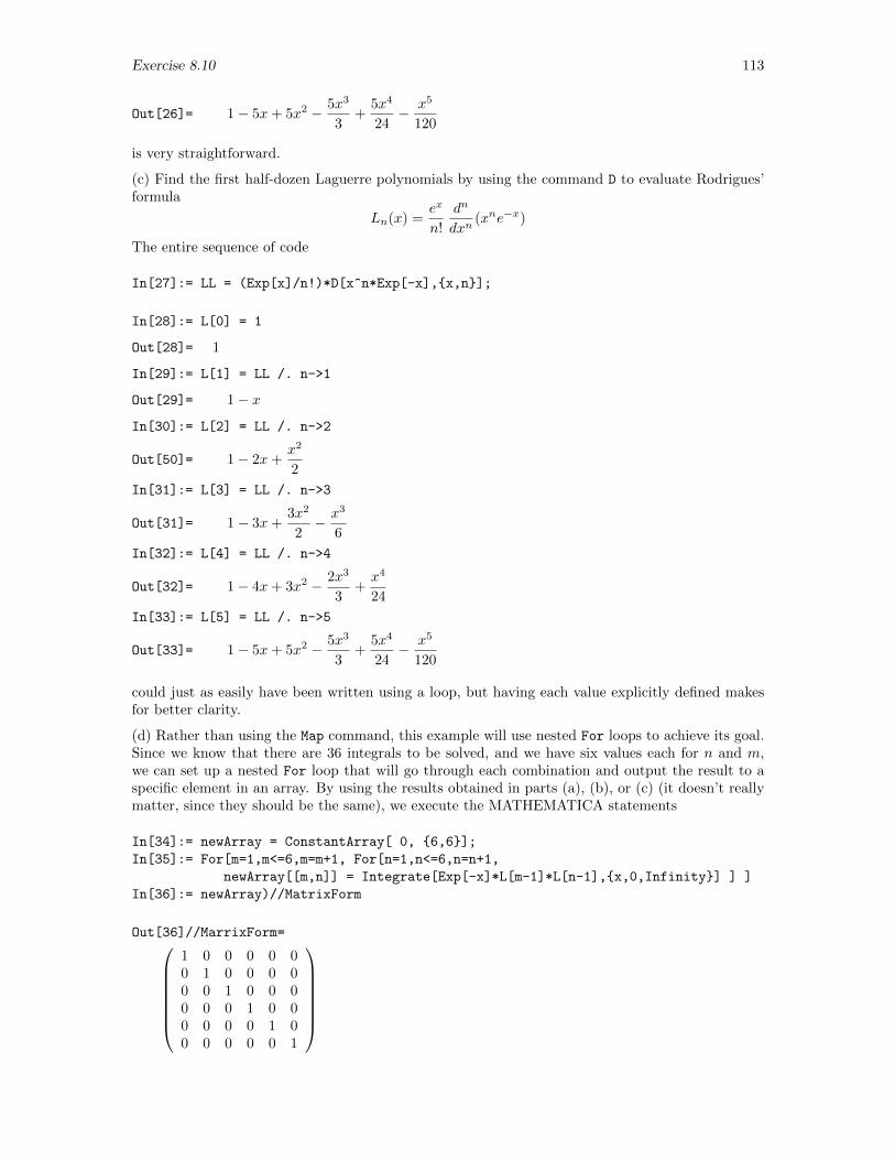
Exercise 8.10 113
Out[26]= 1− 5x+ 5x2 − 5x3
3+
5x4
24− x5
120
is very straightforward.
(c) Find the first half-dozen Laguerre polynomials by using the command D to evaluate Rodrigues’formula
Ln(x) =ex
n!
dn
dxn(xne−x)
The entire sequence of code
In[27]:= LL = (Exp[x]/n!)*D[x^n*Exp[-x],x,n];
In[28]:= L[0] = 1
Out[28]= 1
In[29]:= L[1] = LL /. n->1
Out[29]= 1− x
In[30]:= L[2] = LL /. n->2
Out[50]= 1− 2x+x2
2
In[31]:= L[3] = LL /. n->3
Out[31]= 1− 3x+3x2
2− x3
6
In[32]:= L[4] = LL /. n->4
Out[32]= 1− 4x+ 3x2 − 2x3
3+x4
24
In[33]:= L[5] = LL /. n->5
Out[33]= 1− 5x+ 5x2 − 5x3
3+
5x4
24− x5
120
could just as easily have been written using a loop, but having each value explicitly defined makesfor better clarity.
(d) Rather than using the Map command, this example will use nested For loops to achieve its goal.Since we know that there are 36 integrals to be solved, and we have six values each for n and m,we can set up a nested For loop that will go through each combination and output the result to aspecific element in an array. By using the results obtained in parts (a), (b), or (c) (it doesn’t reallymatter, since they should be the same), we execute the MATHEMATICA statements
In[34]:= newArray = ConstantArray[ 0, 6,6];
In[35]:= For[m=1,m<=6,m=m+1, For[n=1,n<=6,n=n+1,
newArray[[m,n]] = Integrate[Exp[-x]*L[m-1]*L[n-1],x,0,Infinity] ] ]
In[36]:= newArray)//MatrixForm
Out[36]//MarrixForm=1 0 0 0 0 00 1 0 0 0 00 0 1 0 0 00 0 0 1 0 00 0 0 0 1 00 0 0 0 0 1
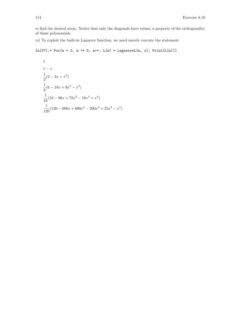
114 Exercise 8.10
to find the desired array. Notice that only the diagonals have values, a property of the orthogonalityof these polynomials.
(e) To exploit the built-in Laguerre function, we need merely execute the statement
In[37]:= For[n = 0, n <= 5, n++, L[n] = LaguerreL[n, x]; Print[L[n]]]
1
1− x1
2(2− 4x+ x2)
1
6(6− 18x+ 9x2 − x3)
1
24(24− 96x+ 72x2 − 16x3 + x4)
1
120(120− 600x+ 600x2 − 200x3 + 25x4 − x5)
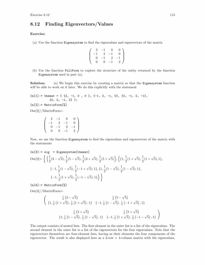
Exercise 8.12 115
8.12 Finding Eigenvectors/Values
Exercise:
(a) Use the function Eigensystem to find the eigenvalues and eigenvectors of the matrix2 −1 0 0−1 2 −1 0
0 −1 2 −10 0 −1 2
(b) Use the function FullForm to explore the structure of the entity returned by the function
Eigensystem used in part (a).
Solution: (a) We begin this exercise by creating a matrix so that the Eigensystem functionwill be able to work on it later. We do this explicitly with the statement
In[1]:= themat = 2, -1, 0 , 0 , -1, 2, -1, 0, 0, -1, 2, -1,
0, 0, -1, 2 ;
In[2]:= MatrixForm[%]
Out[2]//MatrixForm=2 −1 0 0−1 2 −1 0
0 −1 2 −10 0 −1 2
Now, we use the function Eigensystem to find the eigenvalues and eigenvectors of the matrix withthe statements
In[3]:= eig = Eigensystem[themat]
Out[3]=
1
2(3−
√5),
1
2(5−
√5),
1
2(3 +
√5),
1
2(5 +
√5),1, 1
2(1 +
√5),
1
2(1 +
√5), 1,
−1,1
2(1−
√5),
1
2(−1 +
√5), 1, 1, 1
2(1−
√5),
1
2(1−
√5), 1,
−1,1
2(1 +
√5),
1
2(−1−
√5), 1
In[4]:= MatrixForm[%]
Out[4]//MatrixForm=(12
(3−√
5)
12
(5−√
5)
1, 12
(1 +√
5), 1
2
(1 +√
5), 1 −1, 1
2
(1−√
5), 1
2
(−1 +
√5), 1
12
(3 +√
5)
12
(5 +√
5)
1, 12
(1−√
5), 1
2
(1−√
5), 1 −1, 1
2
(1 +√
5), 1
2
(−1−
√5), 1
)
The output consists of nested lists. The first element in the outer list is a list of the eigenvalues. Thesecond element in the outer list is a list of the eigenvectors for the four eigenvalues. Note that theeigenvectors themselves are four-element lists, having as their elements the four components of theeigenvector. The result is also displayed here as a 2-row × 4-column matrix with the eigenvalues,
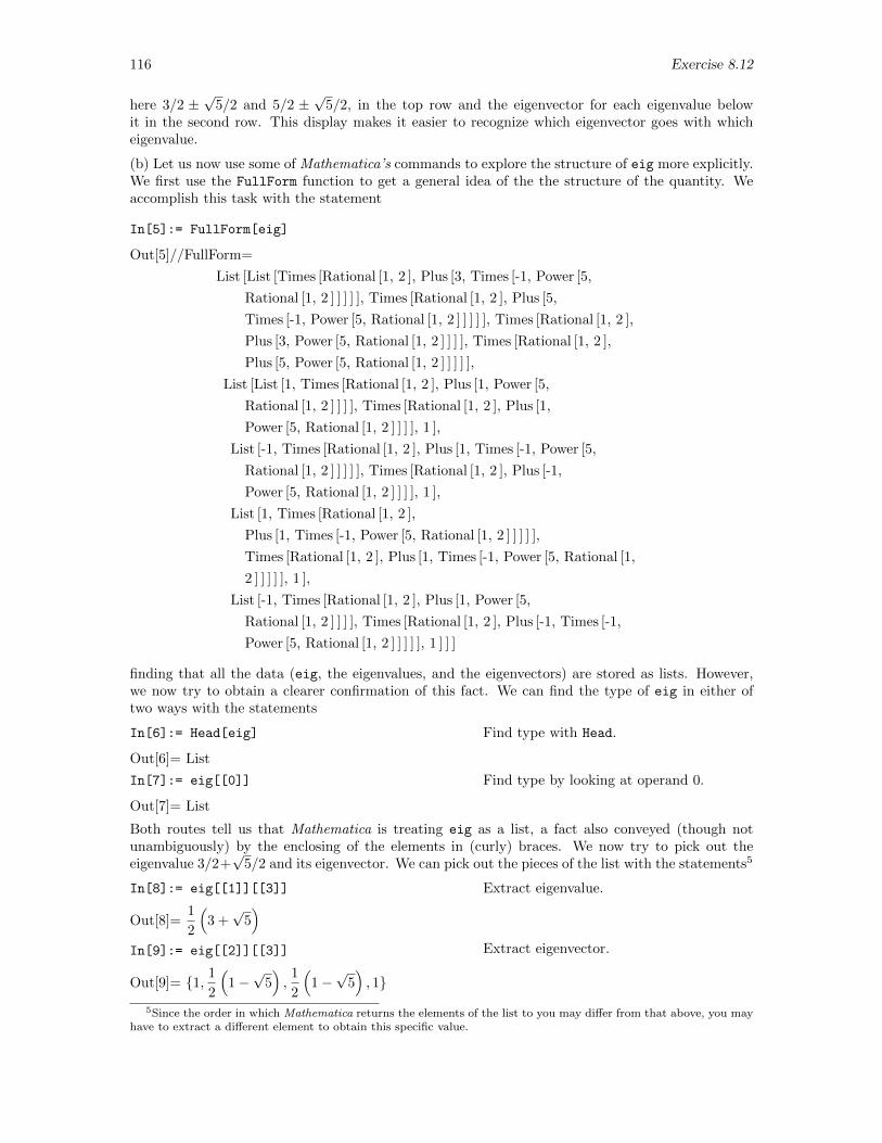
116 Exercise 8.12
here 3/2 ±√
5/2 and 5/2 ±√
5/2, in the top row and the eigenvector for each eigenvalue belowit in the second row. This display makes it easier to recognize which eigenvector goes with whicheigenvalue.
(b) Let us now use some of Mathematica’s commands to explore the structure of eig more explicitly.We first use the FullForm function to get a general idea of the the structure of the quantity. Weaccomplish this task with the statement
In[5]:= FullForm[eig]
Out[5]//FullForm=
List [List [Times [Rational [1, 2 ], Plus [3, Times [-1, Power [5,
Rational [1, 2 ] ] ] ] ], Times [Rational [1, 2 ], Plus [5,
Times [-1, Power [5, Rational [1, 2 ] ] ] ] ], Times [Rational [1, 2 ],
Plus [3, Power [5, Rational [1, 2 ] ] ] ], Times [Rational [1, 2 ],
Plus [5, Power [5, Rational [1, 2 ] ] ] ] ],
List [List [1, Times [Rational [1, 2 ], Plus [1, Power [5,
Rational [1, 2 ] ] ] ], Times [Rational [1, 2 ], Plus [1,
Power [5, Rational [1, 2 ] ] ] ], 1 ],
List [-1, Times [Rational [1, 2 ], Plus [1, Times [-1, Power [5,
Rational [1, 2 ] ] ] ] ], Times [Rational [1, 2 ], Plus [-1,
Power [5, Rational [1, 2 ] ] ] ], 1 ],
List [1, Times [Rational [1, 2 ],
Plus [1, Times [-1, Power [5, Rational [1, 2 ] ] ] ] ],
Times [Rational [1, 2 ], Plus [1, Times [-1, Power [5, Rational [1,
2 ] ] ] ] ], 1 ],
List [-1, Times [Rational [1, 2 ], Plus [1, Power [5,
Rational [1, 2 ] ] ] ], Times [Rational [1, 2 ], Plus [-1, Times [-1,
Power [5, Rational [1, 2 ] ] ] ] ], 1 ] ] ]
finding that all the data (eig, the eigenvalues, and the eigenvectors) are stored as lists. However,we now try to obtain a clearer confirmation of this fact. We can find the type of eig in either oftwo ways with the statements
In[6]:= Head[eig]
Out[6]= List
In[7]:= eig[[0]]
Out[7]= List
Find type with Head.
Find type by looking at operand 0.
Both routes tell us that Mathematica is treating eig as a list, a fact also conveyed (though notunambiguously) by the enclosing of the elements in (curly) braces. We now try to pick out theeigenvalue 3/2+
√5/2 and its eigenvector. We can pick out the pieces of the list with the statements5
In[8]:= eig[[1]][[3]]
Out[8]=1
2
(3 +√
5)
In[9]:= eig[[2]][[3]]
Out[9]= 1, 1
2
(1−√
5),
1
2
(1−√
5), 1
Extract eigenvalue.
Extract eigenvector.
5Since the order in which Mathematica returns the elements of the list to you may differ from that above, you mayhave to extract a different element to obtain this specific value.
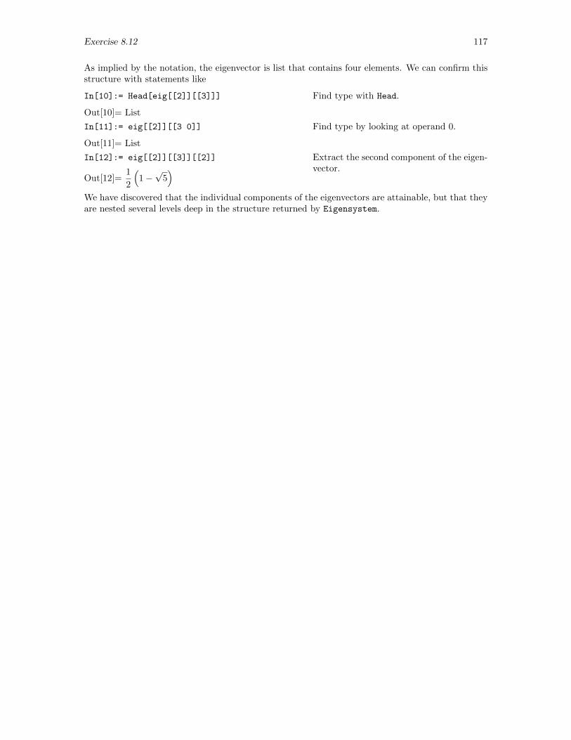
Exercise 8.12 117
As implied by the notation, the eigenvector is list that contains four elements. We can confirm thisstructure with statements like
In[10]:= Head[eig[[2]][[3]]]
Out[10]= List
In[11]:= eig[[2]][[3 0]]
Out[11]= List
In[12]:= eig[[2]][[3]][[2]]
Out[12]=1
2
(1−√
5)
Find type with Head.
Find type by looking at operand 0.
Extract the second component of the eigen-vector.
We have discovered that the individual components of the eigenvectors are attainable, but that theyare nested several levels deep in the structure returned by Eigensystem.
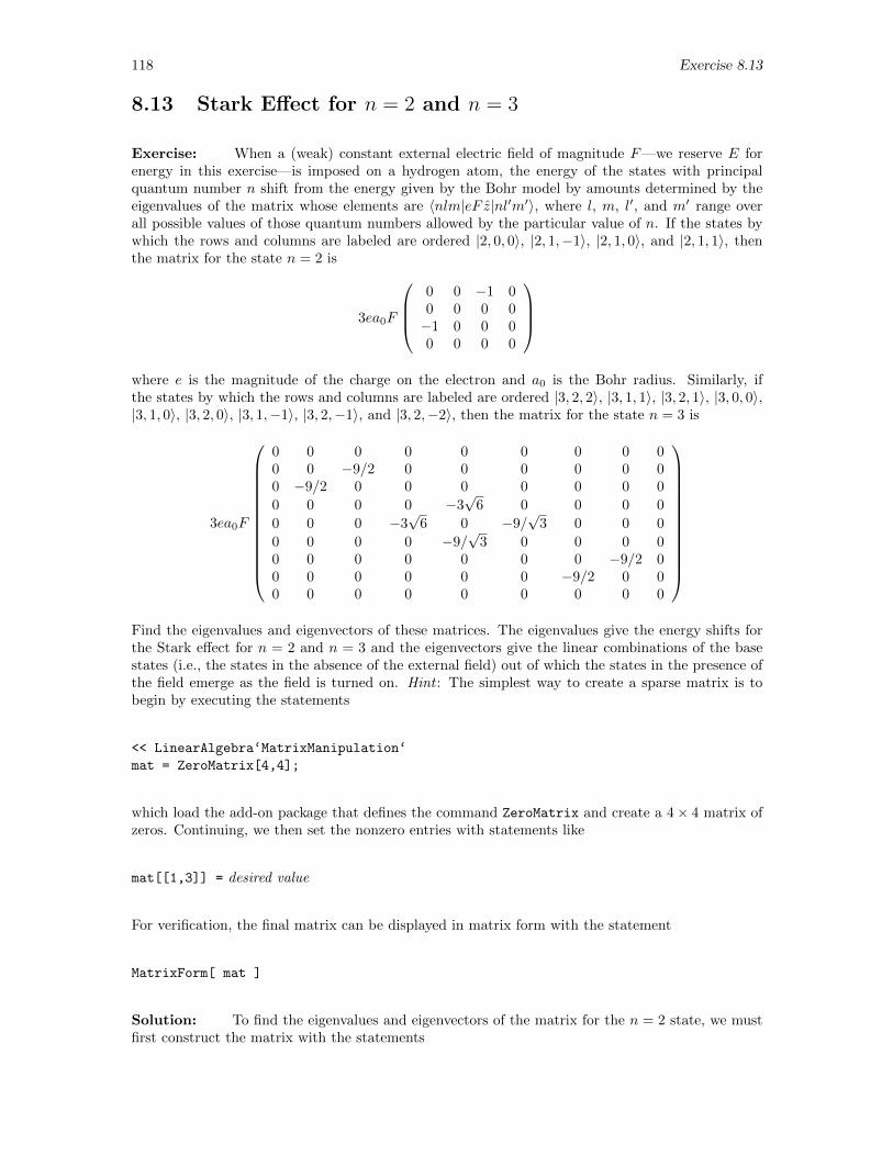
118 Exercise 8.13
8.13 Stark Effect for n = 2 and n = 3
Exercise: When a (weak) constant external electric field of magnitude F—we reserve E forenergy in this exercise—is imposed on a hydrogen atom, the energy of the states with principalquantum number n shift from the energy given by the Bohr model by amounts determined by theeigenvalues of the matrix whose elements are 〈nlm|eF z|nl′m′〉, where l, m, l′, and m′ range overall possible values of those quantum numbers allowed by the particular value of n. If the states bywhich the rows and columns are labeled are ordered |2, 0, 0〉, |2, 1,−1〉, |2, 1, 0〉, and |2, 1, 1〉, thenthe matrix for the state n = 2 is
3ea0F
0 0 −1 00 0 0 0−1 0 0 00 0 0 0
where e is the magnitude of the charge on the electron and a0 is the Bohr radius. Similarly, ifthe states by which the rows and columns are labeled are ordered |3, 2, 2〉, |3, 1, 1〉, |3, 2, 1〉, |3, 0, 0〉,|3, 1, 0〉, |3, 2, 0〉, |3, 1,−1〉, |3, 2,−1〉, and |3, 2,−2〉, then the matrix for the state n = 3 is
3ea0F
0 0 0 0 0 0 0 0 00 0 −9/2 0 0 0 0 0 00 −9/2 0 0 0 0 0 0 0
0 0 0 0 −3√
6 0 0 0 0
0 0 0 −3√
6 0 −9/√
3 0 0 0
0 0 0 0 −9/√
3 0 0 0 00 0 0 0 0 0 0 −9/2 00 0 0 0 0 0 −9/2 0 00 0 0 0 0 0 0 0 0
Find the eigenvalues and eigenvectors of these matrices. The eigenvalues give the energy shifts forthe Stark effect for n = 2 and n = 3 and the eigenvectors give the linear combinations of the basestates (i.e., the states in the absence of the external field) out of which the states in the presence ofthe field emerge as the field is turned on. Hint : The simplest way to create a sparse matrix is tobegin by executing the statements
<< LinearAlgebra‘MatrixManipulation‘
mat = ZeroMatrix[4,4];
which load the add-on package that defines the command ZeroMatrix and create a 4× 4 matrix ofzeros. Continuing, we then set the nonzero entries with statements like
mat[[1,3]] = desired value
For verification, the final matrix can be displayed in matrix form with the statement
MatrixForm[ mat ]
Solution: To find the eigenvalues and eigenvectors of the matrix for the n = 2 state, we mustfirst construct the matrix with the statements
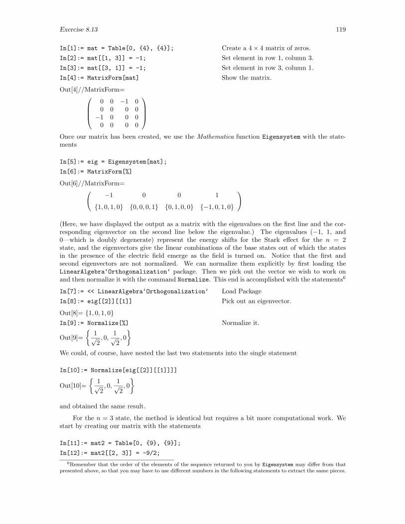
Exercise 8.13 119
In[1]:= mat = Table[0, 4, 4];
In[2]:= mat[[1, 3]] = -1;
In[3]:= mat[[3, 1]] = -1;
In[4]:= MatrixForm[mat]
Out[4]//MatrixForm=0 0 −1 00 0 0 0−1 0 0 0
0 0 0 0
Create a 4× 4 matrix of zeros.
Set element in row 1, column 3.
Set element in row 3, column 1.
Show the matrix.
Once our matrix has been created, we use the Mathematica function Eigensystem with the state-ments
In[5]:= eig = Eigensystem[mat];
In[6]:= MatrixForm[%]
Out[6]//MatrixForm=(−1 0 0 1
1, 0, 1, 0 0, 0, 0, 1 0, 1, 0, 0 −1, 0, 1, 0
)
(Here, we have displayed the output as a matrix with the eigenvalues on the first line and the cor-responding eigenvector on the second line below the eigenvalue.) The eigenvalues (−1, 1, and0—which is doubly degenerate) represent the energy shifts for the Stark effect for the n = 2state, and the eigenvectors give the linear combinations of the base states out of which the statesin the presence of the electric field emerge as the field is turned on. Notice that the first andsecond eigenvectors are not normalized. We can normalize them explicitly by first loading theLinearAlgebra‘Orthogonalization‘ package. Then we pick out the vector we wish to work onand then normalize it with the command Normalize. This end is accomplished with the statements6
In[7]:= << LinearAlgebra‘Orthogonalization‘
In[8]:= eig[[2]][[1]]
Out[8]= 1, 0, 1, 0In[9]:= Normalize[%]
Out[9]=
1√2, 0,
1√2, 0
Load Package
Pick out an eigenvector.
Normalize it.
We could, of course, have nested the last two statements into the single statement
In[10]:= Normalize[eig[[2]][[1]]]]
Out[10]=
1√2, 0,
1√2, 0
and obtained the same result.
For the n = 3 state, the method is identical but requires a bit more computational work. Westart by creating our matrix with the statements
In[11]:= mat2 = Table[0, 9, 9];
In[12]:= mat2[[2, 3]] = -9/2;
6Remember that the order of the elements of the sequence returned to you by Eigensystem may differ from thatpresented above, so that you may have to use different numbers in the following statements to extract the same pieces.
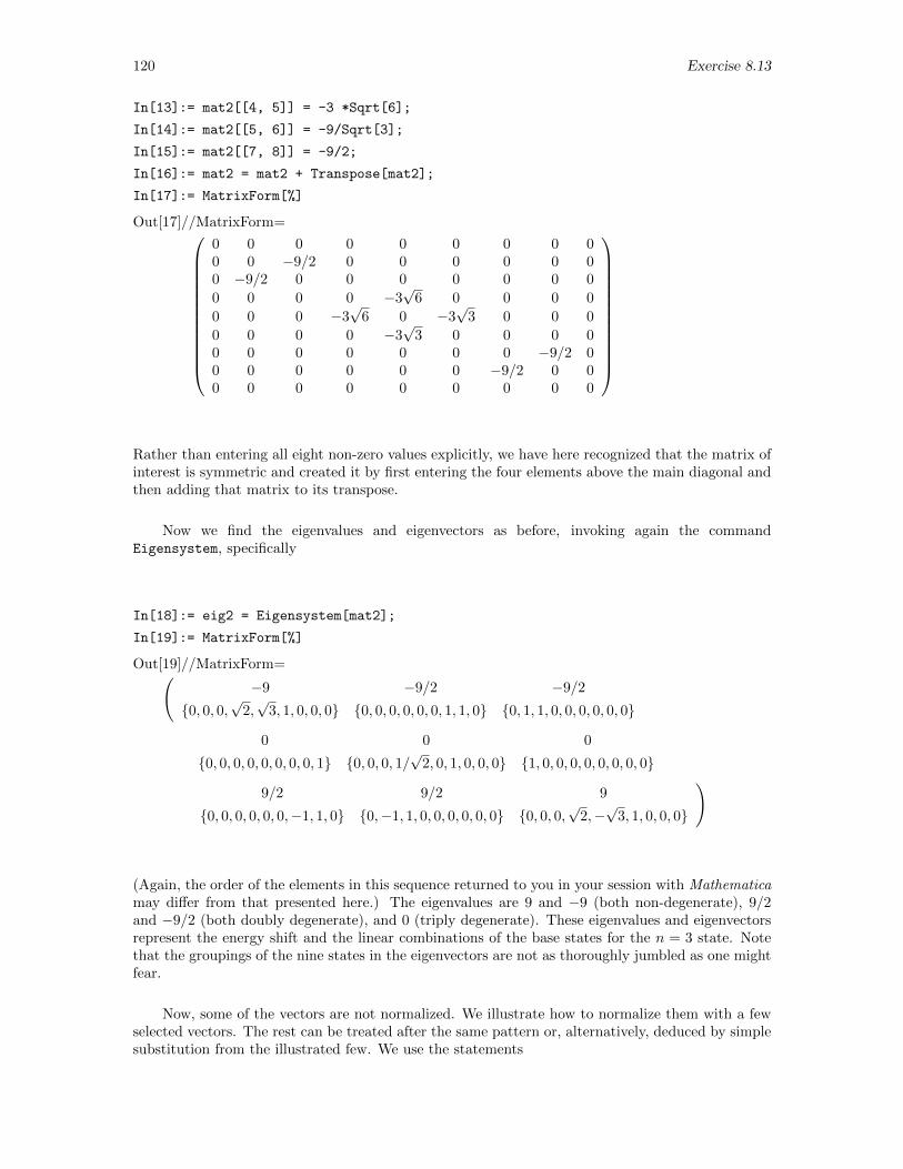
120 Exercise 8.13
In[13]:= mat2[[4, 5]] = -3 *Sqrt[6];
In[14]:= mat2[[5, 6]] = -9/Sqrt[3];
In[15]:= mat2[[7, 8]] = -9/2;
In[16]:= mat2 = mat2 + Transpose[mat2];
In[17]:= MatrixForm[%]
Out[17]//MatrixForm=
0 0 0 0 0 0 0 0 00 0 −9/2 0 0 0 0 0 00 −9/2 0 0 0 0 0 0 0
0 0 0 0 −3√
6 0 0 0 0
0 0 0 −3√
6 0 −3√
3 0 0 0
0 0 0 0 −3√
3 0 0 0 00 0 0 0 0 0 0 −9/2 00 0 0 0 0 0 −9/2 0 00 0 0 0 0 0 0 0 0
Rather than entering all eight non-zero values explicitly, we have here recognized that the matrix ofinterest is symmetric and created it by first entering the four elements above the main diagonal andthen adding that matrix to its transpose.
Now we find the eigenvalues and eigenvectors as before, invoking again the commandEigensystem, specifically
In[18]:= eig2 = Eigensystem[mat2];
In[19]:= MatrixForm[%]
Out[19]//MatrixForm=(−9 −9/2 −9/2
0, 0, 0,√
2,√
3, 1, 0, 0, 0 0, 0, 0, 0, 0, 0, 1, 1, 0 0, 1, 1, 0, 0, 0, 0, 0, 0
0 0 0
0, 0, 0, 0, 0, 0, 0, 0, 1 0, 0, 0, 1/√
2, 0, 1, 0, 0, 0 1, 0, 0, 0, 0, 0, 0, 0, 0
9/2 9/2 9
0, 0, 0, 0, 0, 0,−1, 1, 0 0,−1, 1, 0, 0, 0, 0, 0, 0 0, 0, 0,√
2,−√
3, 1, 0, 0, 0
)
(Again, the order of the elements in this sequence returned to you in your session with Mathematicamay differ from that presented here.) The eigenvalues are 9 and −9 (both non-degenerate), 9/2and −9/2 (both doubly degenerate), and 0 (triply degenerate). These eigenvalues and eigenvectorsrepresent the energy shift and the linear combinations of the base states for the n = 3 state. Notethat the groupings of the nine states in the eigenvectors are not as thoroughly jumbled as one mightfear.
Now, some of the vectors are not normalized. We illustrate how to normalize them with a fewselected vectors. The rest can be treated after the same pattern or, alternatively, deduced by simplesubstitution from the illustrated few. We use the statements
Exercise 8.13 121
In[20]:= eig2[[2]][[9]]
Out[20]= 0, 0, 0,√
2,−√
3, 1, 0, 0, 0
In[21]:= Normalize[eig2[[2]][[9]]]
Out[21]= 0, 0, 0, 1√3,− 1√
2,
1√6, 0, 0, 0
In[22]:= eig2[[2]][[3]]
Out[22]= 0, 1, 1, 0, 0, 0, 0, 0, 0
In[23]:= Normalize[eig2[[2]][[3]]]
Out[23]= 0, 1√2,
1√2, 0, 0, 0, 0, 0, 0
In[24]:= Normalize[eig2[[2]][[2]]]
Out[24]= 0, 0, 0, 0, 0, 0, 1√2,
1√2, 0
In[25]:= Normalize[eig2[[2]][[5]]]
Out[25]= 0, 0, 0,− 1√3, 0,
√2
3, 0, 0, 0
Extract eigenvector belonging to eigenvalue9.
Extract and normalize eigenvector belong-ing to eigenvalue 9
Extract first eigenvector belonging to eigen-value −9/2
Extract and normalize first eigenvector be-longing to eigenvalue −9/2.
Extract and normalize second eigenvectorbelonging to eigenvalue −9/2.
Extract and normalize second eigenvectorbelonging to eigenvalue 0.
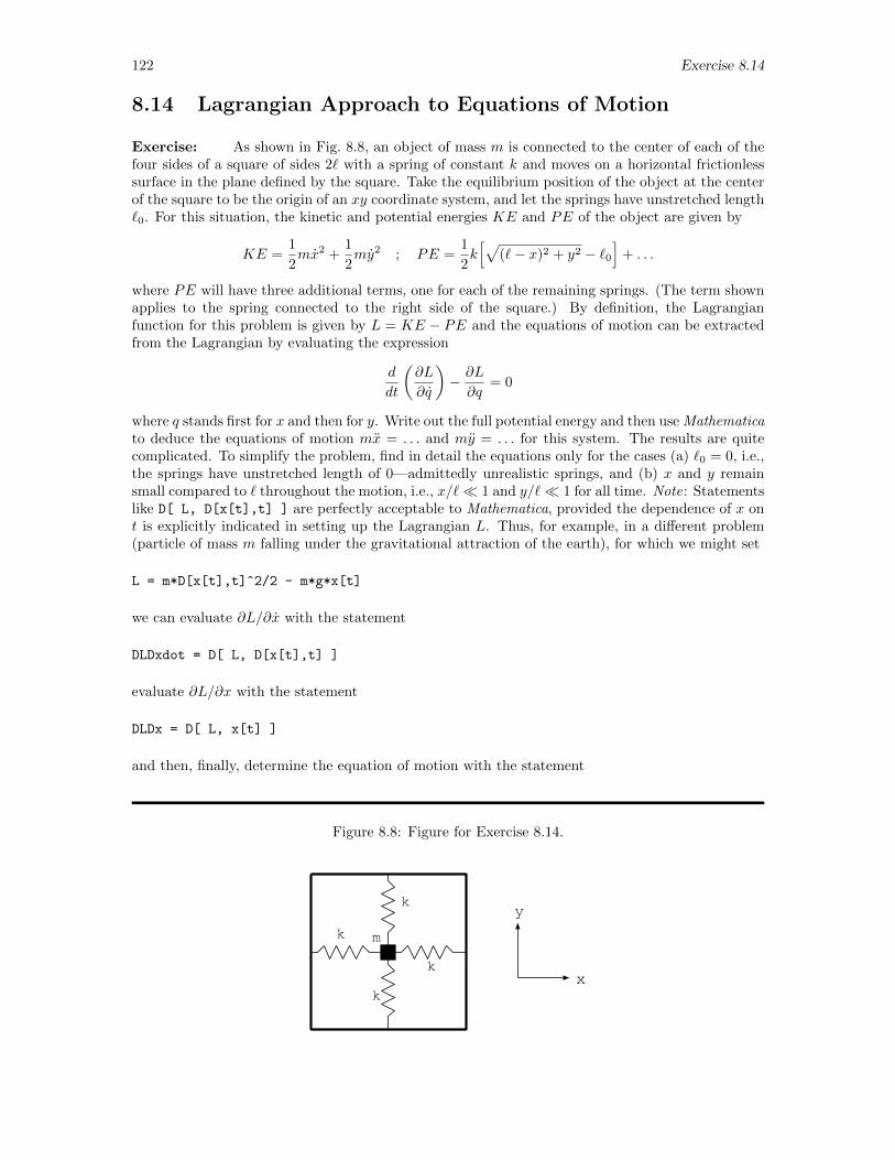
122 Exercise 8.14
8.14 Lagrangian Approach to Equations of Motion
Exercise: As shown in Fig. 8.8, an object of mass m is connected to the center of each of thefour sides of a square of sides 2` with a spring of constant k and moves on a horizontal frictionlesssurface in the plane defined by the square. Take the equilibrium position of the object at the centerof the square to be the origin of an xy coordinate system, and let the springs have unstretched length`0. For this situation, the kinetic and potential energies KE and PE of the object are given by
KE =1
2mx2 +
1
2my2 ; PE =
1
2k[√
(`− x)2 + y2 − `0]
+ . . .
where PE will have three additional terms, one for each of the remaining springs. (The term shownapplies to the spring connected to the right side of the square.) By definition, the Lagrangianfunction for this problem is given by L = KE − PE and the equations of motion can be extractedfrom the Lagrangian by evaluating the expression
d
dt
(∂L
∂q
)− ∂L
∂q= 0
where q stands first for x and then for y. Write out the full potential energy and then use Mathematicato deduce the equations of motion mx = . . . and my = . . . for this system. The results are quitecomplicated. To simplify the problem, find in detail the equations only for the cases (a) `0 = 0, i.e.,the springs have unstretched length of 0—admittedly unrealistic springs, and (b) x and y remainsmall compared to ` throughout the motion, i.e., x/` 1 and y/` 1 for all time. Note: Statementslike D[ L, D[x[t],t] ] are perfectly acceptable to Mathematica, provided the dependence of x ont is explicitly indicated in setting up the Lagrangian L. Thus, for example, in a different problem(particle of mass m falling under the gravitational attraction of the earth), for which we might set
L = m*D[x[t],t]^2/2 - m*g*x[t]
we can evaluate ∂L/∂x with the statement
DLDxdot = D[ L, D[x[t],t] ]
evaluate ∂L/∂x with the statement
DLDx = D[ L, x[t] ]
and then, finally, determine the equation of motion with the statement
Figure 8.8: Figure for Exercise 8.14.
k
k
k
k m
x
y
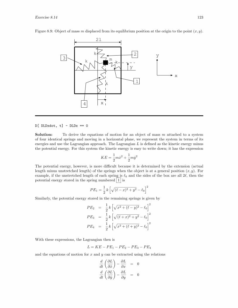
Exercise 8.14 123
Figure 8.9: Object of mass m displaced from its equilibrium position at the origin to the point (x, y).
k
k
kk m
x
y
x
y
2l
1
23
4
D[ DLDxdot, t] - DLDx == 0
Solution: To derive the equations of motion for an object of mass m attached to a systemof four identical springs and moving in a horizontal plane, we represent the system in terms of itsenergies and use the Lagrangian approach. The Lagrangian L is defined as the kinetic energy minusthe potential energy. For this system the kinetic energy is easy to write down; it has the expression
KE =1
2mx2 +
1
2my2
The potential energy, however, is more difficult because it is determined by the extension (actuallength minus unstretched length) of the springs when the object is at a general position (x, y). Forexample, if the unstretched length of each spring is `0 and the sides of the box are all 2`, then thepotential energy stored in the spring numbered 1 is
PE1 =1
2k[√
(`− x)2 + y2 − `0]2
Similarly, the potential energy stored in the remaining springs is given by
PE2 =1
2k[√
x2 + (`− y)2 − `0]2
PE3 =1
2k[√
(`+ x)2 + y2 − `0]2
PE4 =1
2k[√
x2 + (`+ y)2 − `0]2
With these expressions, the Lagrangian then is
L = KE − PE1 − PE2 − PE3 − PE4
and the equations of motion for x and y can be extracted using the relations
d
dt
(∂L
∂x
)− ∂L
∂x= 0
d
dt
(∂L
∂y
)− ∂L
∂y= 0
124 Exercise 8.14
Note here that the equations of motion for both x and y will be (essentially) identical, since rotatingour coordinate system 90 degrees will not change how the problem looks. So, once the equation ofmotion for x is derived, the equation of motion for y can be obtained simply by replacing x with y.
Our first step, then, is to construct the Lagrangian, which we do in several steps with thestatements7
In[1]:= KE = m* xdot^2/2 + m*ydot^2/2;
In[2]:= PE1 = k*(Sqrt[(l - x)^2 + y^2] - l0)^2/2;
In[3]:= PE2 = k*(Sqrt[(l - y)^2 + x^2] - l0)^2/2;
In[4]:= PE3 = k*(Sqrt[(l + x)^2 + y^2] - l0)^2/2;
In[5]:= PE4 = k*(Sqrt[(l + y)^2 + x^2] - l0)^2/2;
In[6]:= L = KE - PE1 - PE2 - PE3 - PE4
Set kinetic energy.
Set potential energy in spring 1.
Set potential energy in spring 2.
Set potential energy in spring 3.
Set potential energy in spring 4.
Evaluate Lagrangian.
Out[6]=mx2
2− 1
2k(−l0 +
√x2 + (l − y)2
)2
− 1
2k(−l0 +
√(l − x)2 + y2
)2
−
1
2k(−l0 +
√(l + x)2 + y2
)2
− 1
2k(−l0 +
√x2 + (l + y)2
)2
+my2
2
Following the suggestion in the statement of the exercise, we then find the equations of motion,starting with the statements
In[7]:= dLdxdot = D[L, xdot]
Out[7]= mx
In[8]:= dLdx = D[L, x]
Out[8]= −kx(−l0 +
√x2 + (l − y)2
)√x2 + (l − y)2
+k (l − x)
(−l0 +
√(l − x)2 + y2
)√
(l − x)2 + y2−
k (l + x)(−l0 +
√(l + x)2 + y2
)√
(l + x)2 + y2−kx(−l0 +
√x2 + (l + y)2
)√x2 + (l + y)2
In[9]:= dLdydot = D[L, ydot]
Out[9]= my
In[10]:= dLdy = D[L, y]
Out[10]= −k(−l0 +
√x2 + (l − y)2
)(l − y)√
x2 + (l − y)2+ky(−l0 +
√(l − x)2 + y2
)√
(l − x)2 + y2−
ky(−l0 +
√(l + x)2 + y2
)√
(l + x)2 + y2−k (l + y)
(−l0 +
√x2 + (l + y)2
)√x2 + (l + y)2
These results are far too complicated to support a simple treatment from here on. To illustrate thestrategy that we would adopt if we really wanted to know the general equations of motion, we focusinstead on two special cases.
Case 1: Suppose that the natural (unstretched) length of the springs is in fact 0, i.e., suppose that`0 = 0. Then, somewhat surprisingly, the Lagrangian and its derivatives reduce to
In[11]:= L1 = L /. l0 -> 0;
7We suppress the output from the first five lines because it is already displayed earlier in this solution.
Exercise 8.14 125
In[12]:= L1 = Expand[L1]
Out[12]= −2kl2 − 2kx2 +mx2
2− 2ky2 +
my2
2
In[13]:= dL1dxdot = D[L1, xdot]
Out[13]= mx
In[14]:= dL1dx = D[L1, x]
Out[14]= −4kx
In[15]:= dL1dydot = D[L1, ydot]
Out[15]= my
In[16]:= dL1dy = D[L1, y]
Out[16]= −4ky
That the complicated expressions should simplify so dramatically in this admittedly idealized situ-ation is a bit of a surprise.
These equations are, of course, not yet the equations of motion. We need to bring the realindependent variable t into greater prominence so we can take the next step. To that end, we makethe replacements
In[17]:= dL1dxdot = dL1dxdot /. x -> x[t], xdot -> D[x[t], t]
Out[17]= mx′[t]
In[18]:= dL1dx = dL1dx /. x -> x[t], xdot -> D[x[t], t]
Out[18]= −4kx[t]
In[19]:= dL1dydot = dL1dydot /. y -> y[t], ydot -> D[y[t], t]
Out[19]= my′[t]
In[20]:= dL1dy = dL1dy /. y -> y[t], ydot -> D[y[t], t]
Out[20]= −4ky[t]
Finally, we find the equations of motion themselves with the statements
In[21]:= eq1 = D[dL1dxdot, t] - dL1dx == 0
Out[21]= 4kx[t] +mx′′[t] == 0
In[22]:= eq2 = D[dL1dydot, t] - dL1dy == 0
Out[22]= 4ky[t] +my′′[t] == 0
These equations are uncoupled and—though the exercise didn’t ask for solutions—are readily solvedand simplified with the statements
In[23]:= DSolve[eq1, eq2, x[t], y[t], t];
In[24]:= % /. Sqrt[k]/Sqrt[m] -> \[Omega]
Out[24]=
x[t]→ C[1] cos(2tω) + C[2] sin(2tω), y[t]→ C[3] cos(2tω) + C[4] sin(2tω)
Here, C[1], C[2], C[3], and C[4] represent constants that would be determined had we been givena set of initial conditions to fulfill. We conclude that, when the springs are identical and have zero
126 Exercise 8.14
unstretched length, the motion of the object consists of SHM in both the x and y directions and thefrequency of both components of the motion is 2ω = 2
√k/m.
Case 2: Suppose that the amplitude of the motion in each coordinate direction is small comparedto ` so that we can linearize the equations of motion once we have them. That is, suppose wecan ignore terms in the equations of motion that involve x2, y2, xy, and higher powers of thedependent variables. Equivalently, since the equations of motion are determined by differentiatingthe Lagrangian with respect to x and y, we can find the equations of motion in this limiting case notby finding the general equations of motion and then linearizing them but more easily by expandingthe Lagrangian to include terms that are quadratic in x and y and then deducing the equations ofmotion. Indeed, for this case, the kinetic energy KE is already quadratic in the significant variables,so we need do nothing to simplify it. We determine the potential energy by itself and then simplifyit with the statements
In[25]:= PE = PE1 + PE2 + PE3 + PE4;
In[26]:= Series[PE, x, 0, 3, y, 0, 3];
In[27]:= Simplify[%, l > 0];
In[28]:= Collect[%, x, y];
In[29]:= PE = ExpandAll[%]
Find potential energy.
Evaluate successive Taylor expansions toinclude terms through x2 and y2.Simplify the result.
Collect powers of x and y.
Expand the result.
Out[29]= 2kl2 − 4kll0 + 2kl02 + 2kx2 − kl0x
2
l+ 2ky2 − kl0y
2
l− 2kl0x
2y2
l3
Note one further simplification that needs to be made to the result. Since Mathematica performedthe Taylor expansions in y after the Taylor expansion in x instead of concurrently, the program didnot recognize that the x2y2 term is negligible compared to the other terms. In other words, sincethe x2y2 term is the same order of some terms that have already been ignored, this term is negligibleand can also be ignored. We perform this operation with the statements
In[30]:= PE = PE /. -(2*k*l0*x^2*y^2)/(l^3) -> 0;
In[31]:= PE = Collect[%, x, y]
Out[31]= 2kl2 − 4kll0 + 2kl02 +
(2k − kl0
l
)x2 +
(2k − kl0
l
)y2
In this special case, the Lagrangian and its derivatives reduce to
In[32]:= L2 = KE - PE
Out[32]= −2kl2 + 4kll0 − 2kl02 −
(2k − kl0
l
)x2 +
mx2
2−(
2k − kl0l
)y2 +
my2
2
In[33]:= dL2dxdot = D[L2, xdot]
Out[33]= mx
In[34]:= dL2dx = Simplify[D[L2, x]]
Out[34]=2k (−2l + l0) x
l
In[35]:= dL2dydot = D[L2, ydot]
Out[35]= my
In[36]:= dL2dy = Simplify[D[L2, y]]
Out[36]=2k (−2l + l0) y
l
Exercise 8.14 127
As in the first special case, these equations are also not yet the equations of motion. We needto bring the real independent variable t into greater prominence so we can take the next step. Tothat end, we make the replacements
In[37]:= dL2dxdot = dL2dxdot /. x -> x[t], xdot -> D[x[t], t]
Out[37]= mx′[t]
In[38]:= dL2dx = dL2dx /. x -> x[t], xdot -> D[x[t], t]
Out[38]=2k (−2l + l0) x[t]
l
In[39]:= dL2dydot = dL2dydot /. y -> y[t], ydot -> D[y[t], t]
Out[39]= my′[t]
In[40]:= dL2dy = dL2dy /. y -> y[t], ydot -> D[y[t], t]
Out[40]=2k (−2l + l0) y[t]
l
Finally, we find the equations of motion themselves with the statements
In[41]:= eq1 = D[dL2dxdot, t] - dL2dx == 0
Out[41]=−2k (−2l + l0) x[t]
l+mx′′[t] = 0
In[42]:= eq2 = D[dL2dydot, t] - dL2dy == 0
Out[42]=−2k (−2l + l0) y[t]
l+my′′[t] = 0
These equations are uncoupled and can be readily solved just as we did for the case l0 = 0. We neednot, however, find that solution explicitly to conclude, to no particular surprise, that the motion ineach coordinate direction is simple harmonic and that the frequency of the motion is the same inboth directions—a frequency given by
Ω =
√2k
m
(2− `0
`
)= ω
√2
(2− `0
`
)= 2ω
√1− `0
2`
where, again, ω =√k/m. In particular, this expression reduces to 2ω when `0 = 0, a result
consistent with that deduced in the previous example. More generally, the frequency of (small-amplitude) oscillations depends on the relationship between the unstretched length of the spring`0 and the side of the box 2`. If, for example, `0 = `, i.e., the spring is neither stretched norcompressed when the object is in its equilibrium position, then the frequency reduces to Ω =
√2ω,
a result consistent with the conclusion that, in those circumstances, only the two springs parallel toone side affect the motion in a direction parallel to that side.
128 Exercise 8.16
8.16 Elliptic Integrals
Exercise: The complete elliptic integrals of the first and second kinds are given by
K(k) =
∫ π/2
0
dφ
(1− k2 sin2 φ)1/2; E(k) =
∫ π/2
0
(1− k2 sin2 φ)1/2 dφ
Use Mathematica to evaluate these integrals to O(k6) by expanding the integrands in Taylor seriesbefore evaluating the integrals.
Solution: In this exercise, we will look at both the Mathematica solutions to the ellipticintegrals and the Taylor approximations of these integrals. To start we define variables and evaluatethe integrals giving K and E by the statements
In[1]:= Kint = 1/Sqrt[1 - k^2*Sin[\[Phi]]^2]
Out[1]=1√
1− k2 sin(φ)2
In[2]:= Kser = Series[ Kint, k, 0, 5 ]
Out[2]= 1 +1
2sin(φ)2k2 +
3
8sin(φ)4k4 +O(k)6
In[3]:= Kpoly = Normal[Integrate[Kser,
\[Phi], 0, Pi/2]]
Out[3]=π
2+k2π
8+
9k4π
128
In[4]:= Eint = Sqrt[1 - k^2*Sin[\[Phi]]^2]
Out[4]=√
1− k2 sin(φ)2
In[5]:= Eser = Series[Eint, k, 0, 5]
Out[5]= 1− 1
2sin(φ)2k2 − 1
8sin(φ)4k4 +O(k)6
In[6]:= Epoly = Normal[Integrate[Eser,
\[Phi], 0, Pi/2]]
Out[6]=π
2− k2π
8− 3k4π
128
Assign variable for K integrand.
Expand the K integrand in a Taylor Series.
Integrate, converting result from a series toa polynomial.
Assign variable for E integrand.
Expand the E integrand in a Taylor Series.
Integrate, converting result from a series toa polynomial.
Now we are ready to generate a graph showing not only the Taylor approximations but also theevaluations built in to Mathematica. We invoke the single statement
In[7]:= Plot[Kpoly, Epoly, EllipticK[k^2], EllipticE[k^2], k, -1.0, 1.0,
PlotRange -> 1, 2.4, AxesLabel -> "k", "E,K",
PlotStyle -> Dashing[0.02, 0.02], Dashing[0.02, 0.02],
Thickness[0.001], Thickness[0.001]]
The display produced by this statement is shown in Fig. 8.10. It shows that the Taylor approximationdoesn’t quite agree with the more precise solution that Mathematica provides for the integrals. Thisis because the Taylor series is built to approximate the equation very close to 0, so one shouldn’texpect it to match for larger k. Even so, to the resolution of the graphs, the Taylor approximationto the order to which we have carried it appears to be good to about k = 0.6!
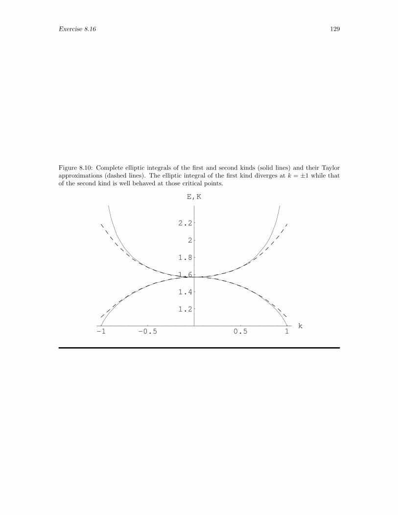
Exercise 8.16 129
Figure 8.10: Complete elliptic integrals of the first and second kinds (solid lines) and their Taylorapproximations (dashed lines). The elliptic integral of the first kind diverges at k = ±1 while thatof the second kind is well behaved at those critical points.
-1 -0.5 0.5 1k
1.2
1.4
1.6
1.8
2
2.2
E,K
130 Exercise 8.17 (Mathematica)
8.17 Laplace transforms
Exercise: Find the Laplace transform of each of the functions
(a) f(t) = tn (b) f(t) = t e−at (c) f(t) = cosh(at) (d)df(t)
dt
and the inverse Laplace transform of each of the functions
(e) f(s) =a+ bs
s2 + ω2(f) f(s) =
a
(s2 + 9ω2)(s2 + 4ω2)(s2 + ω2)
In (c), you may have to express the hyperbolic cosine in exponential form while in (f) you may haveto help Mathematica’s routine InverseLaplaceTransform by first invoking the command Apart toexpand the desired function in partial fractions.
Solution: (a) The Laplace transform of
f(t) = tn
is obtained in Mathematica with the statements
In[1]:= t^n
Out[1]= tn
In[2]:= LaplaceTransform[ %, t, s ]
Out[2]= s−1−nGamma[1 + n]
(b) Forf(t) = te−at
the statements evaluating the Laplace transform are
In[3]:= t*Exp[-a*t]
Out[3]= e−att
In[4]:= LaplaceTransform[ %, t, s ]
Out[4]=1
(a+ s)2
(c) Forf(t) = cosh (at)
the statements evaluating the Laplace transform are
In[5]:= Cosh[a*t]
Out[5]= Cosh[at]
In[6]:= LaplaceTransform[ %, t, s ]
Out[6]=s
−a2 + s2
(d) The inverse Laplace transform of
f(s) =a+ bs
s2 + ω2
is obtained with the statements
Exercise 8.17 (Mathematica) 131
In[7]:= (a + b*s)/(s^2 + \[Omega]^2)
Out[7]=a+ bs
s2 + ω2
In[8]:= InverseLaplaceTransform[ %, s, t ]
Out[8]= b cos [tω] +a sin [tω]
ω
(e) Finally, if
f(s) =a
(s2 + 9ω2)(s2 + 4ω2)(s2 + ω2)
the inverse Laplace transform is obtained quickly with the statements
In[9]:= qs = a/((s^2 + 9*\[Omega]^2)(s^2 + 4*\[Omega]^2)(s^2 + \[Omega]^2))
Out[9]=a
(s2 + 9ω2)(s2 + 4ω2)(s2 + ω2)
In[10]:= qt = InverseLaplaceTransform[ %, s, t ]
Out[10]=4aCos [tω/2) Sin [tω/2]
5
15ω5
Alternatively, we might obtain the result in a more conventional form by first expanding f(s) inpartial fractions in s2, finding that
In[11]:= qs1 = Apart[ qs, s^2 ]
Out[11]= :=a
24ω4(s2 + ω2)− a
15ω4(s2 + 4ω2)+
a
40ω4(s2 + 9ω2)
Then, remembering from the table in Section 2 of the chapter on solving ordinary differential equa-tions that the inverse Laplace transform of ω/(s2 + ω2) is sin(ωt), we recognize that each of theterms in this expression can be inverted separately to give a simple sine function with an appropriate(constant) multiplier and an appropriate argument. With this form of the transform, Mathematica’sinversion routine will automatically treat each term separately, and we find that
In[12]:= qt1 := InverseLaplaceTransform[ qs1, s, t ]
Out[12]=aSin [tω]
24ω5− aCos [tω] Sin [tω]
15ω5+a Sin [3tω]
120ω5
To cast this result in an even more conventional form, we could invoke the statement
In[13]:= Map[ TrigReduce, qt1 ]
Out[13]=aSin [tω]
24ω5− a Sin [2tω]
30ω5+a Sin [3tω]
120ω5
and, to show the agreement of this form with the form obtained first, we would invoke the statement
In[14]:= Simplify[ qt1 ]
Out[14]=4aCos [tω/2) Sin [tω/2]
5
15ω5
132 Exercise 8.18
8.18 Fitting Parabola Through Three Points
Exercise: Given the three points (xi, yi), i = 1, 2, 3, (a) find symbolic expressions for thecoefficients a, b, and c of the parabola y = ax2 + bx+ c that passes through these three points andthen (b) find a symbolic expression for the value of x at which the extreme point of the parabolaoccurs. Finally, (c) determine numerically the angle at which the maximum range of a projectileoccurs if the ranges at θ = 39, 40, and 41 are 0.7251744, 0.729383, and 0.7258887, respectively.
Solution: (a) The equation y = ax2 + bx + c relates the five quantities x, y, a, b, and c.Given three points (xi, yi), i = 1, 2, 3, through which this parabola must pass, we can create threeindependent equations and solve for a, b, and c with the Mathematica commands
In[1]:= GenEq = y == a*x^2 + b*x + c;
In[2]:= Eq1 = GenEq /. x -> x1, y -> y1;
In[3]:= Eq2 = GenEq /. x -> x2, y -> y2;
In[4]:= Eq3 = GenEq /. x -> x3, y -> y3;
In[5]:= soln = Solve[Eq1, Eq2, Eq3,
a, b, c]
Define the general equation.Create an equation for point 1.Create an equation for point 2.Create an equation for point 3.Solve the system of linear equations for thecoefficients a, b, and c.
Out[5] =
a→ − x2y3 − x3y2 − x1y3 − x2y1 + x1y2 + x3y1
−x2x23 + x1x2
3 − x1x22 + x3x2
2 − x3x21 + x2x2
1
,
b→ −x21y3 + x2
1y2 + y1x23 − y1x
22 + x2
2y3 − y2x23
−x2x23 + x1x2
3 − x1x22 + x3x2
2 − x3x21 + x2x2
1
,
c→ y2x1x23 − x2
1x3y2 − x22x1y3 + x2
2x3y1 + x21x2y3 − y1x2x
23
−x2x23 + x1x2
3 − x1x22 + x3x2
2 − x3x21 + x2x2
1
These parameters define the parabola passing through the three specified points.
(b) If we want to find where the maximum value of x is for the given parabola, we need only lookat the singular point where the derivative of our parabolic equation is 0. We must assume of coursethat a 6= 0. Then we can solve this equation for x to find xmax. In Mathematica the statementsused for making the substitution and solving for xmax are
In[6]:= NewGenEq = GenEq /. soln;
In[7]:= DiffGenEq = D[NewGenEq, x];
In[8]:= xmax = Solve[DiffGenEq, x]
Substitute the representations for the vari-ables from soln obtained in part (a) to cre-ate the new equation.Differentiate that equation. (Here, since wedid not specify y as a variable of x its deriva-tive is 0).Solve the differentiated equation for x.
Out[8] =
x→ −x2
1y3 + x21y2 + y1x
23 − y1x
22 + x2
2y3 − y2x23
2(x2y3 − x3y2 − x1y3 − x2y1 + x1y2 + x3y1)
(c) Upon inspecting the data given here, we expect the maximum range to occur at an initial anglesomewhere between 39 and 41. From (b) we know if we are given any three pairs of input andoutput we can find the extreme value of x on a parabola via direct substitution. We expect that,for the values listed, the maximum value will occur at an angle between 39 and 41. To find theangle at which the maximum occurs for the values listed, we use the Mathematica statement
In[9]:= xmax /. x1 -> 39, x2 -> 40, x3 -> 41, y1 -> 0.7251744, y2 -> 0.729383,
y3 -> 0.7258887
Out[9]=
x→ 40.0464
The result tells us that, if we desire the maximum range, we should fire the projectile at an initialangle of 40.0464. As we expected, the result falls between 39 and 41.
Exercise 8.19 133
8.19 Deducing Simpson’s Rule
Exercise: Find symbolic expressions for the coefficients a, b, and c that will cause the parabolay = ax2 + bx+ c to pass through the three points (x1 = x2− δx, y1), (x2, y2), and x3 = x2 + δx, y3).Then integrate the parabola over the interval x1 ≤ x ≤ x3 and deduce Simpson’s rule∫ x3
x1
y(x) dx =δx
3
(y1 + 4y2 + y3
)Solution: In an expression containing five variables such as y = ax2 + bx+ c, we need at leastthree equations containing different explicit values for two of the variables. Here, we have threesets of points for x and y, so the task is to define the three equations for the three separate points,solve the system of linear equations for the variables a, b, and c, then integrate the new quadraticequation from x1 to x3. In Mathematica this involves starting with the statements
In[1]:= eqn1 = y1 == a * (x2 - dx)^2 + b*(x2 - dx) + c;
In[2]:= eqn2 = y2 == a*x2^2 + b*x2 + c;
In[3]:= eqn3 = y3 == a * (x2 + dx)^2 + b*(x2 + dx) + c;
In[4]:= soln = Solve[eqn1, eqn2, eqn3, a, b, c]
Out[4]=
a→ −−y1 + 2y2 − y3
2 dx2,
b→ −dx y1 + 2x2y1 − 4x2y2 − dx y3 + 2x2y3
2dx2
c→ −dxx2y1 − x22y1 − 2 dx2y2 + 2x2
2y2 + dxx2y3 − x22y3
2 dx2
We have solved our system of linear equations. Now we need construct the approximating parabolaby assigning a, b, and c to the values generated in this solution and then evaluating the expressiongiving y. To those ends, we invoke the statements
In[5]:= a = soln[[1, 1, 2]];
In[6]:= b = soln[[1, 2, 2]];
In[7]:= c = soln[[1, 3, 2]];
In[8]:= y = a*x^2 + b*x + c
Out[8]= −x2 (−y1 + 2y2 − y3)
2 dx2 − x (dx y1 + 2x2y1 − 4x2y2 − dx y3 + 2x2y3)
2 dx2 −
−dxx2y1 − x22y1 − 2 dx2y2 + 2x2
2y2 + dxx2y3 − x22y3
2 dx2
We next integrate and recast this expression with the statements
In[9]:= Integrate[y, x, x2 - dx, x2 + dx]
Out[9]=dx y1
3+
4 dx y2
3+dx y3
3
In[10]:= Factor[%]
Out[10]=1
3dx (y1 + 4y2 + y3)
We have deduced Simpson’s rule using Mathematica.
134 Exercise 8.20
8.20 Accuracy of Simpson’s Rule
Exercise: The midpoint rule M and Simpson’s rule S for evaluating integrals numerically startwith the assumptions that∫ b
a
f(x) dx ≈M = (b− a) f
(a+ b
2
);
∫ b
a
f(x) dx ≈ S =b− a
6
(f(a) + 4 f
(a+ b
2
)+ f(b)
)respectively. To deduce the first of these expressions, we approximate f(x) over the interval a ≤ x ≤ bwith a constant equal to the value of f(x) at the midpoint of the interval while deducing the secondentails approximating the function with a quadratic polynomial that passes through f(x) at theendpoints and the midpoint of the interval. The midpoint rule will clearly be 100% accurate iff(x) is a constant and Simpson’s rule will be 100% accurate if f(x) is a quadratic polynomial. Usesymbolic manipulation to show that, surprisingly, the midpoint rule is in fact 100% accurate forthe linear function f(x) = mx + p and Simpson’s rule is 100% accurate for the cubic polynomialf(x) = cx3 + dx2 + ex + g! Optional : Try to construct geometric arguments that would provideinsight into the correctness of these analytic results.
Solution: The midpoint rule for evaluating integrals numerically is exact for linear functions,as we can show with the statements
In[1]:= linf[x_] := m*x + p
In[2]:= intab = Integrate[linf[x], x, a, b]
Out[2]= −a2m
2+b2m
2− ap+ bp
In[3]:= (b - a)*linf[(a + b)/2];
In[4]:= intmid = Expand[%]
Out[4]= −a2m
2+b2m
2− ap+ bp
Clearly the result obtained by integrating the linear function is equivalent to the result obtained byapplying the midpoint rule, though we could make this result even more evident either by subtractingone value from the other with the statement
In[5]:= Simplify[ intmid - intab ]
Out[5]= 0
or by asking whether they are equal with the statement
In[6]:= intmid == intab
Out[6]= True
This result makes sense for a linear function. Geometrically, the value of the integral given by themidpoint rule is the area under the rectangle in Fig. 8.11 while the integral of the linear functionis the area under the inclined line in that figure. The area under the horizontal line overestimatesthe area under the inclined line in the first half of the interval of integration and underestimatesthat area in the second half of the interval of integration, but the overestimate in the first half of theinterval is exactly the same as the underestimate in the second half of the interval. The two errorscancel and the end result is exactly correct.
In the same way, Simpson’s rule is exact for cubic polynomials, as we can check with thestatements
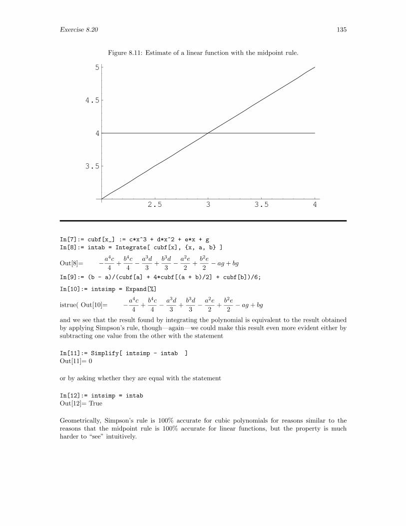
Exercise 8.20 135
Figure 8.11: Estimate of a linear function with the midpoint rule.
2.5 3 3.5 4
3.5
4
4.5
5
In[7]:= cubf[x_] := c*x^3 + d*x^2 + e*x + g
In[8]:= intab = Integrate[ cubf[x], x, a, b ]
Out[8]= −a4c
4+b4c
4− a3d
3+b3d
3− a2e
2+b2e
2− ag + bg
In[9]:= (b - a)/(cubf[a] + 4*cubf[(a + b)/2] + cubf[b])/6;
In[10]:= intsimp = Expand[%]
istrue( Out[10]= −a4c
4+b4c
4− a3d
3+b3d
3− a2e
2+b2e
2− ag + bg
and we see that the result found by integrating the polynomial is equivalent to the result obtainedby applying Simpson’s rule, though—again—we could make this result even more evident either bysubtracting one value from the other with the statement
In[11]:= Simplify[ intsimp - intab ]
Out[11]= 0
or by asking whether they are equal with the statement
In[12]:= intsimp = intab
Out[12]= True
Geometrically, Simpson’s rule is 100% accurate for cubic polynomials for reasons similar to thereasons that the midpoint rule is 100% accurate for linear functions, but the property is muchharder to “see” intuitively.
136 Exercise 8.24
8.24 Vector Derivatives in Cylindrical Coordinates
Exercise: Using the functions Grad, Laplacian, Div, and Curl defined in Section 8.8.10,
a. Evaluate the gradient of (i.e., the negative of the force field associated with) each of thefunctions
V1(r, φ, z) =1
(r2 + z2)1/2V2(r, φ, z) =
z
(r2 + z2)3/2
V3(r, φ, z) =2z2 − r2
(r2 + z2)5/2V4(r, φ, z) =
e−a(r2+z2)1/2
(r2 + z2)1/2
of the cylindrical variables r (radial), φ (azimuthal), and z (axial).
b. Verify that each field obtained in part (a) is conservative by showing that the curl of each iszero.
c. With r = r r + z k, show (1) that ∇× r = 0 and (2) that ∇ • r = 3.
d. With V5(r, φ, z) = r2 + z2, show that ∇2V5(r, φ, z) = ∇ •∇V5(r, φ, z) = 6.
e. Show that ∇2V1(r, φ, z) = 0. (Note: Except at r = z = 0.)
f. Evaluate the Laplacian of V4(r, φ, z), ∇2V4(r, φ, z).
Solution: We begin by defining the several functions referred to in this exercise with thestatements
In[1]:= V1 = 1/Sqrt[r^2+z^2];
In[2]:= V2 = z/(r^2+z^2)^(3/2);
In[3]:= V3 = (2*z^2 - r^2)/(r^2+z^2)^(5/2);
In[4]:= V4 = Exp[-a*Sqrt[r^2+z^2] ]/Sqrt[r^2+z^2];
In[5]:= V5 = r^2 + z^2;
(a) We evaluate the several gradients with the statements
In[6]:= gradV1 = Grad[V1, r,\[Phi],z, "Cylindrical"]
Out[6]=
− r
(r2 + z2)3/2, 0,− z
(r2 + z2)3/2
In[7]:= gradV2 = Grad[V2, r,\[Phi],z, "Cylindrical"]
Out[7]=
− 3rz
(r2 + z2)5/2, 0,− 3z2
(r2 + z2)5/2+
1
(r2 + z2)3/2
In[8]:= gradV3 = Grad[V3, r,\[Phi],z, "Cylindrical"]
Out[8]=
− 2r
(r2 + z2)5/2− 5r(−r2 + 2z2)
(r2 + z2)7/2, 0,
4z
(r2 + z2)5/2− 5z(−r2 + 2z2)
(r2 + z2)7/2
In[9]:= gradV4 = Grad[V4, r,\[Phi],z, "Cylindrical"]
Out[9]=
− r
(r2 + z2)3/2− ar
r2 + z2, 0,− az
r2 + z2− z
(r2 + z2)3/2
e−a√r2+z2
(b) Next, we evaluate the curl of each of the results in part (a) with the statements
Exercise 8.24 137
In[10]:= Curl[gradV1, r,\[Phi],z, "Cylindrical"]
Out[10]= 0,0,0
In[11]:= Curl[gradV2, r,\[Phi],z, "Cylindrical"]
Out[11]= 0,0,0
In[12]:= Curl[gradV3, r,\[Phi],z, "Cylindrical"]
Out[12]= 0,0,0
In[13]:= Curl[gradV4, r,\[Phi],z, "Cylindrical"]
Out[13]= 0,0,0
Clearly, each of the potentials V1, V2, V3 and V4 is gives rise to a conservative force field.
(c) The curl and divergence of the position vector are evaluated with the statements
In[14]:= poscyl = r,0,z
Out[14]= r, 0, zIn[15]:= Curl[ poscyl, r,\[Phi],z, "Cylindrical" ]
Out[15]= 0,0,0
In[16]:= Div[ poscyl, r,\[Phi],z, "Cylindrical" ]
Out[16]= 3
(d) The Laplacian of V5, which is the square of the distance of the point from the origin, is addressedwith the statement
In[17]) Laplacian[ r^2+z^2, r,\[Phi],z, "Cylindrical" ]
Out[17]= 6
or with the statement
In[18]:= Div[ Grad[ r^2+z^2, r,phi,z, "Cylindrical"],
r,\[Phi],z, "Cylindrical" ]
Out[18]= 6
(e) Since ∇2V1 = ∇ •∇V1 and ∇V1 was evaluated as gradV1 above, the single statement
In[19]:= Div[ gradV1, r,phi,z, "Cylindrical" ]
Out[19]= A bit of a mess In[20]:= Factor[%]
Out[20]= 0
Note that it took a few tries before finding that the command Factor achieved the desired simplifi-cation.
(f) Similarly to (e), ∇2V4 = ∇•∇V4 and ∇V4 was evaluated as gradV4 above, the single statement
In[21]:= Div[ gradV4, r,phi,z, "Cylindrical" ]
Out[21]= A bit of a messIn[22]:= Factor(%)
Out[22]=a2 e−a
√r2+z2
√r2 + z2
Alternatively, we could use the function Laplacian with the statement

138 Exercise 8.24
In[23]:= Laplacian[ V4, r,phi,z, "Cylindrical" ]
Out[23]= A bit of a messIn[24]:= Factor(%)
Out[24]=a2 e−a
√r2+z2
√z2 + r2
Exercise 8.26 139
8.26 Vector Product Identities
Exercise: Create four three-component vectors A, B, CC, and DD with statements like8
A = A1, A2, A3; B = B1,B2,B3; CC = CC1,CC2,CC3; DD = DD1,DD2,DD3;
Then, using the file crossdot.m as described in Section 8.11, show that
a. A×B = −B×A, or, equivalently, that A×B + B×A = 0.
b. A×(B×CC
)=(A •CC
)B−
(A •B
)CC
c.(A×B
)×CC =
(A •CC
)B−
(B •CC
)A
d. A •(B×CC
)=(A×B
)•CC
e.(A×B
)•(CC×DD
)=(A •CC
)(B •DD
)−(A •DD
)(B •CC
)Solution: After launching MATHEMATICA and setting the default directory to the directorycontaining the desired file, we load the MATHEMATICA command file crossdot.m and define thefour vectors with the statements
In[1]:= Get[ "crossdot.m" ]
In[2]:= A = A1, A2, A3; B = B1,B2,B3; CC = CC1,CC2,CC3; DD = DD1,DD2,DD3;
a. We evaluate the two cross products with the statements
In[3]:= cross1 = lucross[A,B]
Out[3]= -A3 B2 + A2 B3, A3 B1-A1 B3, -A2 B1 + A1 B2
In[4]:= cross2 = lucross[B,A]
Out[4]= A3 B2-A2 B3, -A3 B1 + A1 B3, A2 B1-A1 B2
and test the assertion that A×B + B×A = 0 with the statement
In[5]:= cross1 + cross2
Out[5]= 0, 0, 0
clearly verifying that A×B = −B×A.
b. In a similar vein, the statements
In[6]:= pt1 = lucross[ A, lucross[B,CC]];
In[7]:= pt2 = ludot[A,CC]*B - ludot[A,B]*CC;
In[8]:= Expand[ pt1 - pt2 ]
Out[8]= 0, 0, 0
verify that A×(B×CC
)=(A •CC
)B−
(A •B
)CC
c. To verify that(A×B
)×CC =
(A •CC
)B−
(B •CC
)A we invoke the statements
In[9]:= exp1 = lucross[lucross[A,B], CC ];
In[10]:= exp2 = ludot[A,CC]*B - ludot[B,CC]*A;
In[11]:= Expand[ exp1 - exp2 ]
Out[11]= 0, 0, 0
8The variables C and D in MATHEMATICA are protected.
140 Exercise 8.26
Comparing parts (b) and (c), we confirm that the position of the parentheses in this so-called triple cross product is important. This particular triple product is not associative, i.e.,A×
(B×CC
)6=(A×B
)×CC.
d. To verify that A •(B×CC
)=(A×B
)•CC we invoke the statements
In[12]:= exp3 = ludot[ A, lucross[B,CC] ];
In[13]:= exp4 = ludot[ lucross[A,B], CC ];
In[14]:= Expand[ exp3 - exp4 ]
Out[14]= 0
Q.E.D.
e. Finally, to verify that(A×B
)•(CC×DD
)=(A •CC
)(B •DD
)−(A •DD
)(B •CC
)we
invoke the statements
In[15]:= exp5 = ludot[ lucross[A,B], lucross[CC,DD] ];
In[16]:= exp6 = ludot[A,CC]*ludot[B,DD] - ludot[A,DD]*ludot[B,CC];
In[17:= Expand[ exp5 - exp6 ]
Out[17]= 0
Q.E.D. Note that this identity can alternatively be written in the form
(A×B
)•(CC×DD
)=
∣∣∣∣ A •CC A •DDB •CC B •DD
∣∣∣∣
Chapter 9
Introduction to Programming
9.2 Relationship between IF-THEN-ELSE and CASE
Exercise: Figure 9.1 shows three different alternative structures. Express each structure using(a) only CASE structures and (b) only IF-THEN-ELSE structures. In these figures, T, F, C, and B
stand for true, false, condition, and block of statements, respectively. Use proper indentation asillustrated in the examples.
Solution: (a) In the pseudocode of Chapter 9, this figure translates directly into the nestedIF-THEN-ELSE control structure
IF C1 THEN B1
ELSE IF C2 THEN B2
ELSE B3
END_IF
END_IF
Equivalently, using the CASE structure, we would write
CASE
OF C1 DO B1
OF C2 DO B2
OF OTHERS DO B3
END_CASE
(b) In the pseudocode of Chapter 9, this figure translates directly into the CASE structure
CASE
OF C1 DO B1
OF C2 DO B2
OF C3 DO B3
OF OTHERS DO B4
END_CASE
Equivalently, using the IF-THEN-ELSE structure, we would write
141
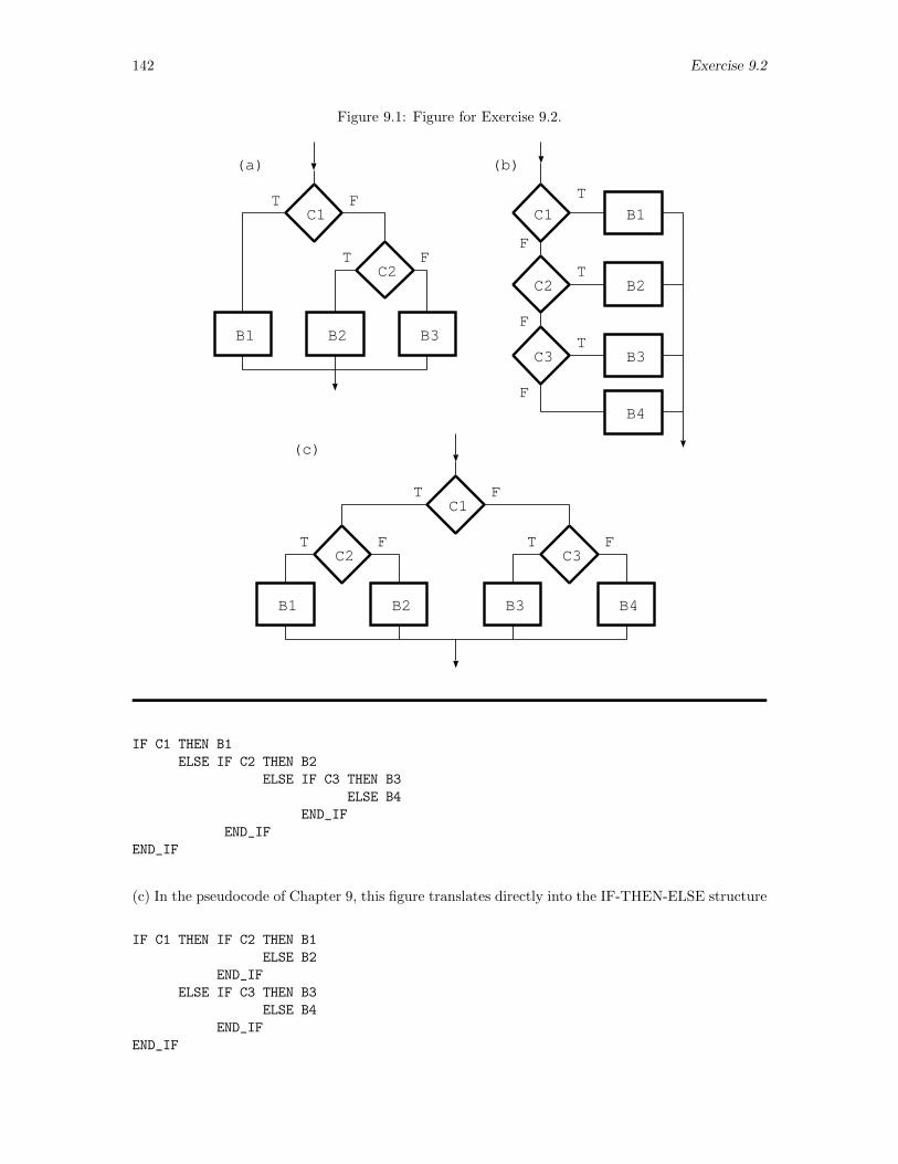
142 Exercise 9.2
Figure 9.1: Figure for Exercise 9.2.
C1
B1
C2
C1
C2
C3
B2 B3
B1
B3
B2
(a)
B4
(b)
C1
C2 C3
B1 B3B2 B4
(c)
T
T
T
T
T T
T
T F
F
F F
F
F
F
F
IF C1 THEN B1
ELSE IF C2 THEN B2
ELSE IF C3 THEN B3
ELSE B4
END_IF
END_IF
END_IF
(c) In the pseudocode of Chapter 9, this figure translates directly into the IF-THEN-ELSE structure
IF C1 THEN IF C2 THEN B1
ELSE B2
END_IF
ELSE IF C3 THEN B3
ELSE B4
END_IF
END_IF
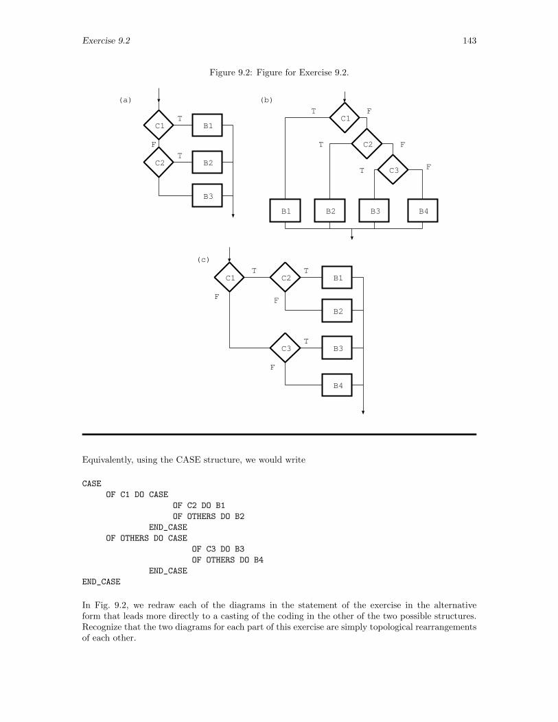
Exercise 9.2 143
Figure 9.2: Figure for Exercise 9.2.
C1 B1
C2
C1
C2
C3B2
B3
B1 B3B2
(a)
B4
(b)
C1 C2
C3
B1
B3
B2
B4
(c)
T
T
T
T T
T
T
T
F F
F
F
F
F
F
Equivalently, using the CASE structure, we would write
CASE
OF C1 DO CASE
OF C2 DO B1
OF OTHERS DO B2
END_CASE
OF OTHERS DO CASE
OF C3 DO B3
OF OTHERS DO B4
END_CASE
END_CASE
In Fig. 9.2, we redraw each of the diagrams in the statement of the exercise in the alternativeform that leads more directly to a casting of the coding in the other of the two possible structures.Recognize that the two diagrams for each part of this exercise are simply topological rearrangementsof each other.
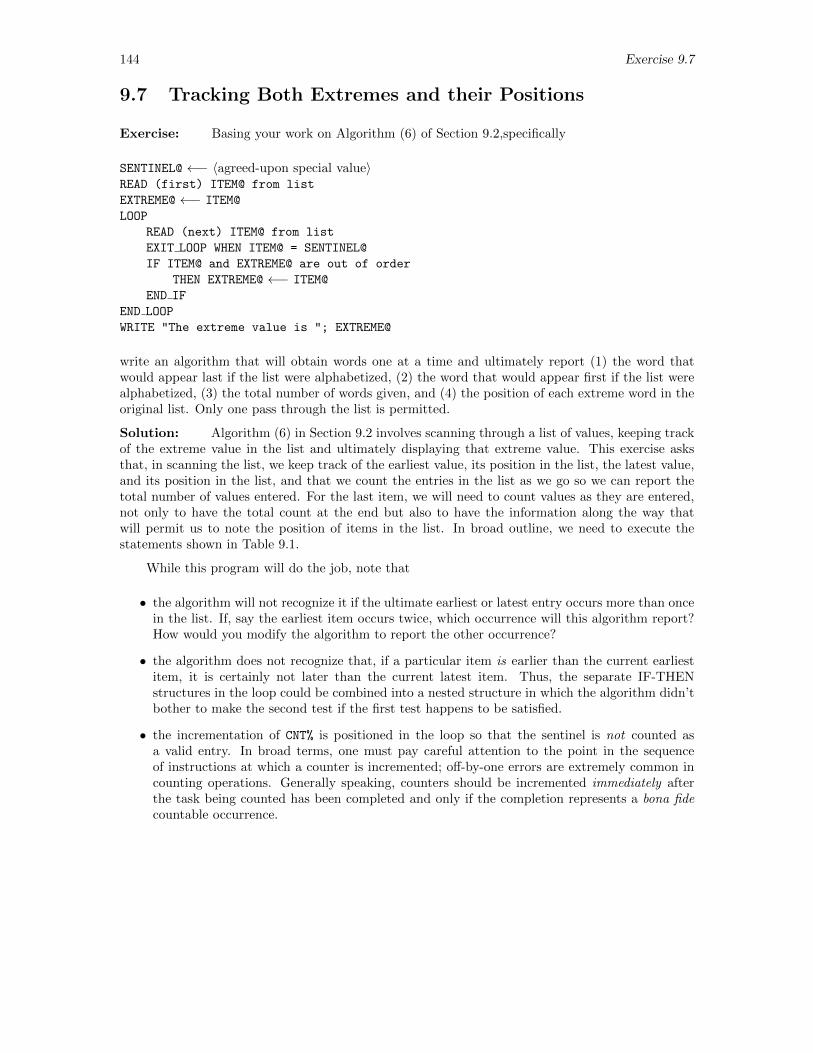
144 Exercise 9.7
9.7 Tracking Both Extremes and their Positions
Exercise: Basing your work on Algorithm (6) of Section 9.2,specifically
SENTINEL@ ←− 〈agreed-upon special value〉READ (first) ITEM@ from list
EXTREME@ ←− ITEM@
LOOP
READ (next) ITEM@ from list
EXIT LOOP WHEN ITEM@ = SENTINEL@
IF ITEM@ and EXTREME@ are out of order
THEN EXTREME@ ←− ITEM@
END IF
END LOOP
WRITE "The extreme value is "; EXTREME@
write an algorithm that will obtain words one at a time and ultimately report (1) the word thatwould appear last if the list were alphabetized, (2) the word that would appear first if the list werealphabetized, (3) the total number of words given, and (4) the position of each extreme word in theoriginal list. Only one pass through the list is permitted.
Solution: Algorithm (6) in Section 9.2 involves scanning through a list of values, keeping trackof the extreme value in the list and ultimately displaying that extreme value. This exercise asksthat, in scanning the list, we keep track of the earliest value, its position in the list, the latest value,and its position in the list, and that we count the entries in the list as we go so we can report thetotal number of values entered. For the last item, we will need to count values as they are entered,not only to have the total count at the end but also to have the information along the way thatwill permit us to note the position of items in the list. In broad outline, we need to execute thestatements shown in Table 9.1.
While this program will do the job, note that
• the algorithm will not recognize it if the ultimate earliest or latest entry occurs more than oncein the list. If, say the earliest item occurs twice, which occurrence will this algorithm report?How would you modify the algorithm to report the other occurrence?
• the algorithm does not recognize that, if a particular item is earlier than the current earliestitem, it is certainly not later than the current latest item. Thus, the separate IF-THENstructures in the loop could be combined into a nested structure in which the algorithm didn’tbother to make the second test if the first test happens to be satisfied.
• the incrementation of CNT% is positioned in the loop so that the sentinel is not counted asa valid entry. In broad terms, one must pay careful attention to the point in the sequenceof instructions at which a counter is incremented; off-by-one errors are extremely common incounting operations. Generally speaking, counters should be incremented immediately afterthe task being counted has been completed and only if the completion represents a bona fidecountable occurrence.
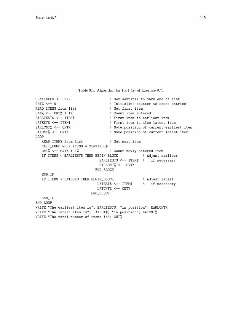
Exercise 9.7 145
Table 9.1: Algorithm for Part (a) of Exercise 9.7.
SENTINEL$ <-- ??? ! Set sentinel to mark end of list
CNT% <-- 0 ! Initialize counter to count entries
READ ITEM$ from list ! Get first item
CNT% <-- CNT% + 1% ! Count item entered
EARLIEST$ <-- ITEM$ ! First item is earliest item
LATEST$ <-- ITEM$ ! First item is also latest item
EARLCNT% <-- CNT% ! Note position of current earliest item
LATCNT% <-- CNT% ! Note position of current latest item
LOOP
READ ITEM$ from list ! Get next item
EXIT_LOOP WHEN ITEM$ = SENTINEL$
CNT% <-- CNT% + 1% ! Count newly entered item
IF ITEM$ < EARLIEST$ THEN BEGIN_BLOCK ! Adjust earliest
EARLIEST$ <-- ITEM$ ! if necessary
EARLCNT% <-- CNT%
END_BLOCK
END_IF
IF ITEM$ > LATEST$ THEN BEGIN_BLOCK ! Adjust latest
LATEST$ <-- ITEM$ ! if necessary
LATCNT% <-- CNT%
END_BLOCK
END_IF
END_LOOP
WRITE "The earliest item is"; EARLIEST$; "in position"; EARLCNT%
WRITE "The latest item is"; LATEST$; "in position"; LATCNT%
WRITE "The total number of items is"; CNT%
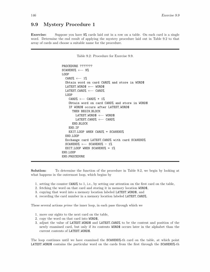
146 Exercise 9.9
9.9 Mystery Procedure 1
Exercise: Suppose you have N% cards laid out in a row on a table. On each card is a singleword. Determine the end result of applying the mystery procedure laid out in Table 9.2 to thatarray of cards and choose a suitable name for the procedure.
Table 9.2: Procedure for Exercise 9.9.
PROCEDURE ???????
SCANEND% ←− N%
LOOP
CARD% ←− 1%
Obtain word on card CARD% and store in WORD$
LATEST WORD$ ←− WORD$
LATEST CARD% ←− CARD%
LOOP
CARD% ←− CARD% + 1%
Obtain word on card CARD% and store in WORD$
IF WORD$ occurs after LATEST WORD$
THEN BEGIN BLOCK
LATEST WORD$ ←− WORD$
LATEST CARD% ←− CARD%
END BLOCK
END IF
EXIT LOOP WHEN CARD% = SCANEND%
END LOOP
Exchange card LATEST CARD% with card SCANEND%
SCANEND% ←− SCANEND% - 1%
EXIT LOOP WHEN SCANEND% = 1%
END LOOP
END PROCEDURE
Solution: To determine the function of the procedure in Table 9.2, we begin by looking atwhat happens in the outermost loop, which begins by
1. setting the counter CARD% to 1, i.e., by setting our attention on the first card on the table,2. fetching the word on that card and storing it in memory location WORD$,3. copying that word into a memory location labeled LATEST WORD$, and4. recording the card number in a memory location labeled LATEST CARD%.
These several actions prime the inner loop, in each pass through which we
1. move our sights to the next card on the table,2. copy the word on that card into WORD$,3. adjust the value of LATEST WORD$ and LATEST CARD% to be the content and position of the
newly examined card, but only if its contents WORD$ occurs later in the alphabet than thecurrent contents of LATEST WORD$.
The loop continues until we have examined the SCANEND%-th card on the table, at which pointLATEST WORD$ contains the particular word on the cards from the first through the SCANEND%-th
Exercise 9.9 147
that occurs latest in the alphabet and LATEST CARD% contains the position on the table of the cardcontaining that word.
Upon exit from the inner loop, we exchange the SCANEND%-th card with the LATEST CARD%-thcard, thereby moving to the SCANEND%-th position the card in the subgroup of cards from 1 thruSCANEND%, i.e., we move the card in that subgroup that will be latest in the alphabet to the lastposition in the subgroup!
Then, we decrement SCANEND% and go back to the beginning of the outermost loop.
Note that the outer loop starts with SCANEND% set to the number of cards on the table. Thus,in the first pass through that outer loop, we move the card in the entire stack that is latest inthe alphabet to the last position in the stack. Then we ignore that last card by decrementingthe counter on the outer loop. At the end of the next pass through the outer loop, we move the“latest-in-the-alphabet” card in the first N%-1% cards to the bottom of that stack. Then, we movethe “latest-in-the-alphabet” card in the first N%-2% cards to the bottom of that stack, . . .. Everytime we move a card, we move the card displaced by the “latest-in-the-alphabet” card to a positionearlier in the stack—so it will continue to be examined in each pass through the loops until suchtime as it, itself, becomes the “latest-in-the-alphabet” card, moves to the bottom, and ceases to befurther examined.
By the time this mystery procedure has completed execution, the cards on the table have beenarranged in alphabetic order.
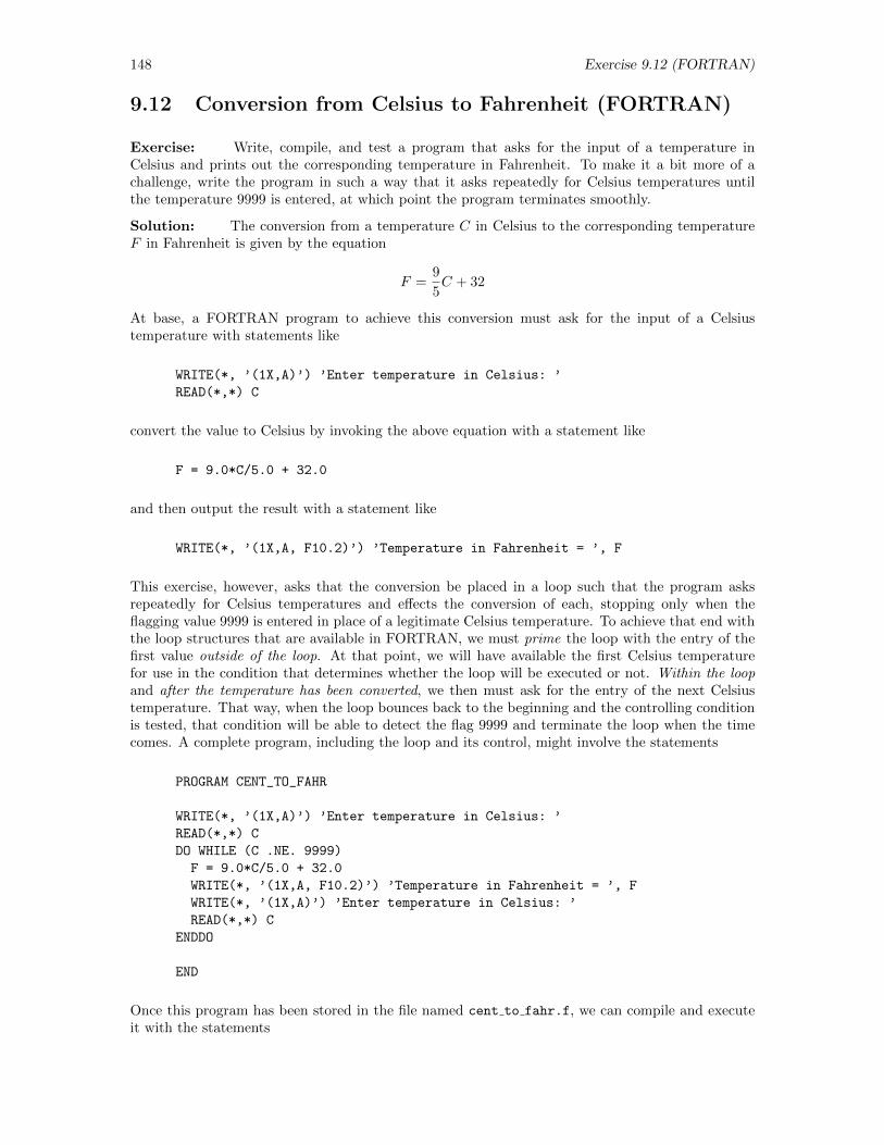
148 Exercise 9.12 (FORTRAN)
9.12 Conversion from Celsius to Fahrenheit (FORTRAN)
Exercise: Write, compile, and test a program that asks for the input of a temperature inCelsius and prints out the corresponding temperature in Fahrenheit. To make it a bit more of achallenge, write the program in such a way that it asks repeatedly for Celsius temperatures untilthe temperature 9999 is entered, at which point the program terminates smoothly.
Solution: The conversion from a temperature C in Celsius to the corresponding temperatureF in Fahrenheit is given by the equation
F =9
5C + 32
At base, a FORTRAN program to achieve this conversion must ask for the input of a Celsiustemperature with statements like
WRITE(*, ’(1X,A)’) ’Enter temperature in Celsius: ’
READ(*,*) C
convert the value to Celsius by invoking the above equation with a statement like
F = 9.0*C/5.0 + 32.0
and then output the result with a statement like
WRITE(*, ’(1X,A, F10.2)’) ’Temperature in Fahrenheit = ’, F
This exercise, however, asks that the conversion be placed in a loop such that the program asksrepeatedly for Celsius temperatures and effects the conversion of each, stopping only when theflagging value 9999 is entered in place of a legitimate Celsius temperature. To achieve that end withthe loop structures that are available in FORTRAN, we must prime the loop with the entry of thefirst value outside of the loop. At that point, we will have available the first Celsius temperaturefor use in the condition that determines whether the loop will be executed or not. Within the loopand after the temperature has been converted, we then must ask for the entry of the next Celsiustemperature. That way, when the loop bounces back to the beginning and the controlling conditionis tested, that condition will be able to detect the flag 9999 and terminate the loop when the timecomes. A complete program, including the loop and its control, might involve the statements
PROGRAM CENT_TO_FAHR
WRITE(*, ’(1X,A)’) ’Enter temperature in Celsius: ’
READ(*,*) C
DO WHILE (C .NE. 9999)
F = 9.0*C/5.0 + 32.0
WRITE(*, ’(1X,A, F10.2)’) ’Temperature in Fahrenheit = ’, F
WRITE(*, ’(1X,A)’) ’Enter temperature in Celsius: ’
READ(*,*) C
ENDDO
END
Once this program has been stored in the file named cent to fahr.f, we can compile and executeit with the statements
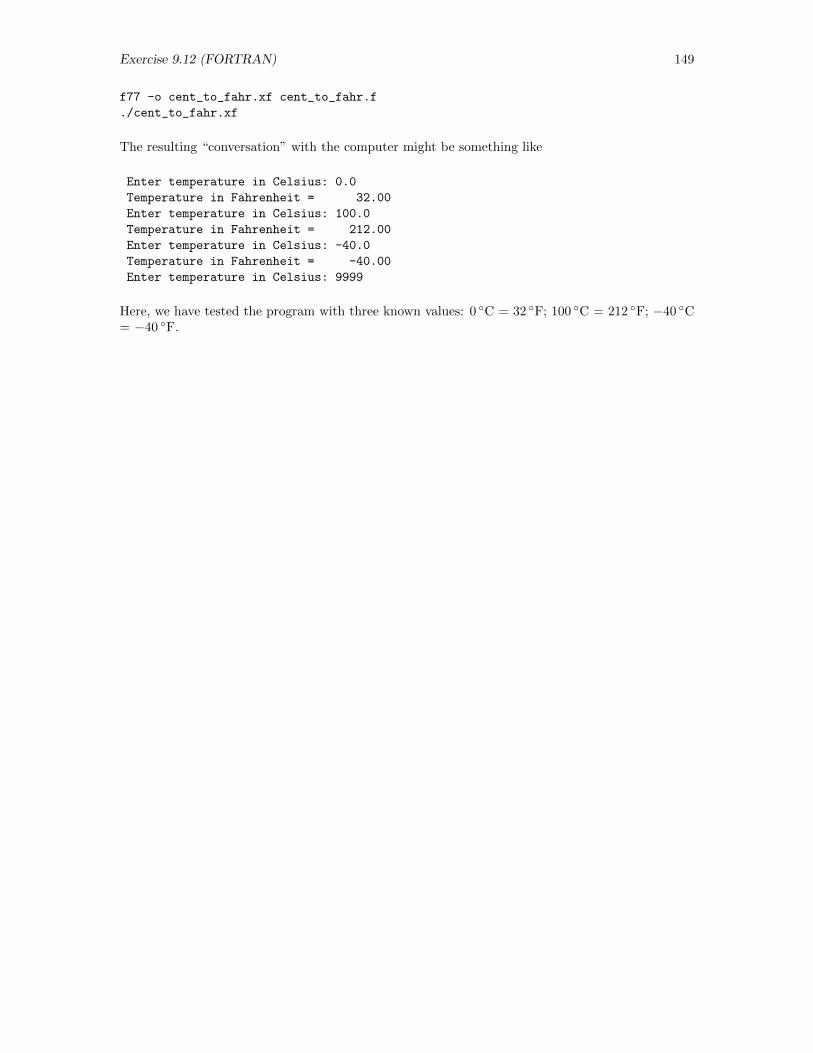
Exercise 9.12 (FORTRAN) 149
f77 -o cent_to_fahr.xf cent_to_fahr.f
./cent_to_fahr.xf
The resulting “conversation” with the computer might be something like
Enter temperature in Celsius: 0.0
Temperature in Fahrenheit = 32.00
Enter temperature in Celsius: 100.0
Temperature in Fahrenheit = 212.00
Enter temperature in Celsius: -40.0
Temperature in Fahrenheit = -40.00
Enter temperature in Celsius: 9999
Here, we have tested the program with three known values: 0 C = 32 F; 100 C = 212 F; −40 C= −40 F.
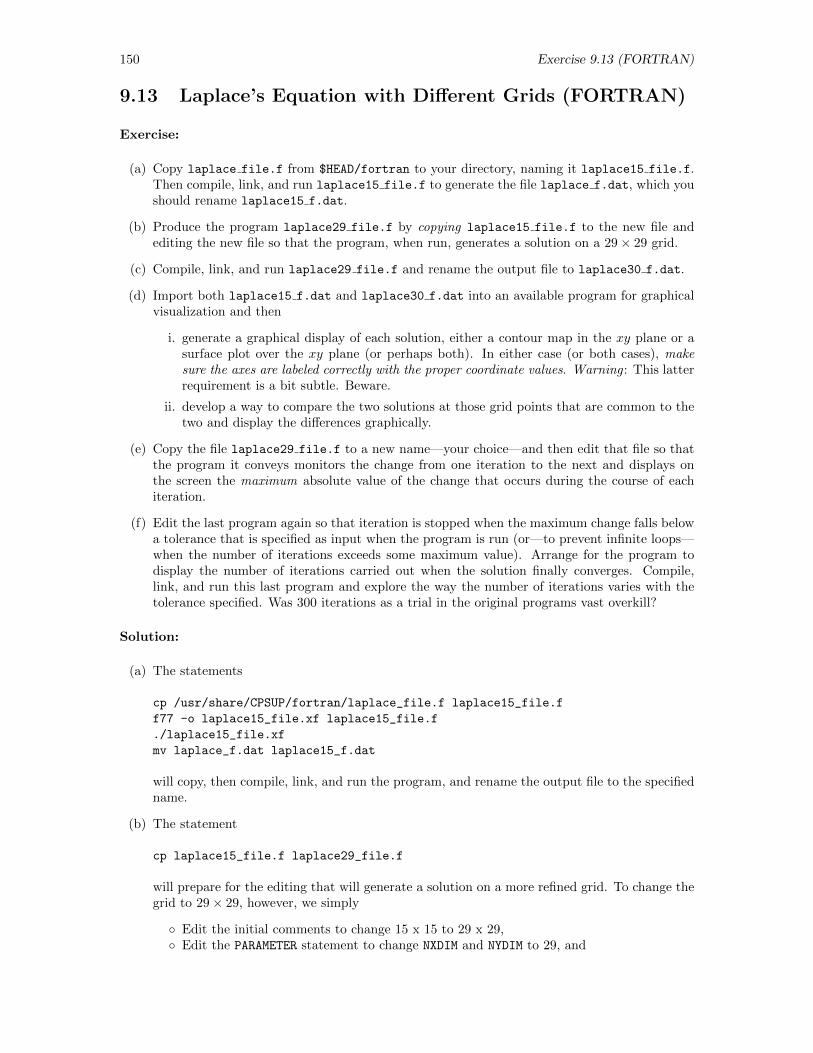
150 Exercise 9.13 (FORTRAN)
9.13 Laplace’s Equation with Different Grids (FORTRAN)
Exercise:
(a) Copy laplace file.f from $HEAD/fortran to your directory, naming it laplace15 file.f.Then compile, link, and run laplace15 file.f to generate the file laplace f.dat, which youshould rename laplace15 f.dat.
(b) Produce the program laplace29 file.f by copying laplace15 file.f to the new file andediting the new file so that the program, when run, generates a solution on a 29× 29 grid.
(c) Compile, link, and run laplace29 file.f and rename the output file to laplace30 f.dat.
(d) Import both laplace15 f.dat and laplace30 f.dat into an available program for graphicalvisualization and then
i. generate a graphical display of each solution, either a contour map in the xy plane or asurface plot over the xy plane (or perhaps both). In either case (or both cases), makesure the axes are labeled correctly with the proper coordinate values. Warning : This latterrequirement is a bit subtle. Beware.
ii. develop a way to compare the two solutions at those grid points that are common to thetwo and display the differences graphically.
(e) Copy the file laplace29 file.f to a new name—your choice—and then edit that file so thatthe program it conveys monitors the change from one iteration to the next and displays onthe screen the maximum absolute value of the change that occurs during the course of eachiteration.
(f) Edit the last program again so that iteration is stopped when the maximum change falls belowa tolerance that is specified as input when the program is run (or—to prevent infinite loops—when the number of iterations exceeds some maximum value). Arrange for the program todisplay the number of iterations carried out when the solution finally converges. Compile,link, and run this last program and explore the way the number of iterations varies with thetolerance specified. Was 300 iterations as a trial in the original programs vast overkill?
Solution:
(a) The statements
cp /usr/share/CPSUP/fortran/laplace_file.f laplace15_file.f
f77 -o laplace15_file.xf laplace15_file.f
./laplace15_file.xf
mv laplace_f.dat laplace15_f.dat
will copy, then compile, link, and run the program, and rename the output file to the specifiedname.
(b) The statement
cp laplace15_file.f laplace29_file.f
will prepare for the editing that will generate a solution on a more refined grid. To change thegrid to 29× 29, however, we simply
Edit the initial comments to change 15 x 15 to 29 x 29, Edit the PARAMETER statement to change NXDIM and NYDIM to 29, and
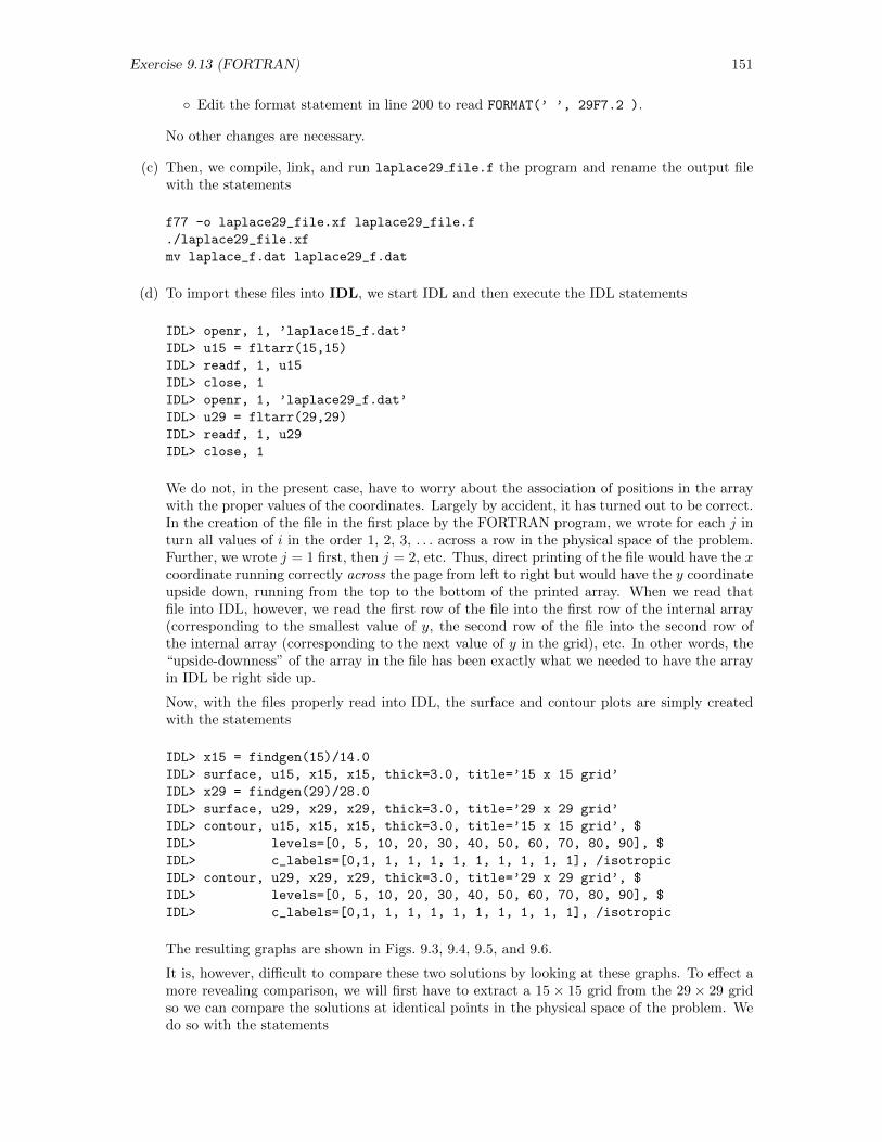
Exercise 9.13 (FORTRAN) 151
Edit the format statement in line 200 to read FORMAT(’ ’, 29F7.2 ).
No other changes are necessary.
(c) Then, we compile, link, and run laplace29 file.f the program and rename the output filewith the statements
f77 -o laplace29_file.xf laplace29_file.f
./laplace29_file.xf
mv laplace_f.dat laplace29_f.dat
(d) To import these files into IDL, we start IDL and then execute the IDL statements
IDL> openr, 1, ’laplace15_f.dat’
IDL> u15 = fltarr(15,15)
IDL> readf, 1, u15
IDL> close, 1
IDL> openr, 1, ’laplace29_f.dat’
IDL> u29 = fltarr(29,29)
IDL> readf, 1, u29
IDL> close, 1
We do not, in the present case, have to worry about the association of positions in the arraywith the proper values of the coordinates. Largely by accident, it has turned out to be correct.In the creation of the file in the first place by the FORTRAN program, we wrote for each j inturn all values of i in the order 1, 2, 3, . . . across a row in the physical space of the problem.Further, we wrote j = 1 first, then j = 2, etc. Thus, direct printing of the file would have the xcoordinate running correctly across the page from left to right but would have the y coordinateupside down, running from the top to the bottom of the printed array. When we read thatfile into IDL, however, we read the first row of the file into the first row of the internal array(corresponding to the smallest value of y, the second row of the file into the second row ofthe internal array (corresponding to the next value of y in the grid), etc. In other words, the“upside-downness” of the array in the file has been exactly what we needed to have the arrayin IDL be right side up.
Now, with the files properly read into IDL, the surface and contour plots are simply createdwith the statements
IDL> x15 = findgen(15)/14.0
IDL> surface, u15, x15, x15, thick=3.0, title=’15 x 15 grid’
IDL> x29 = findgen(29)/28.0
IDL> surface, u29, x29, x29, thick=3.0, title=’29 x 29 grid’
IDL> contour, u15, x15, x15, thick=3.0, title=’15 x 15 grid’, $
IDL> levels=[0, 5, 10, 20, 30, 40, 50, 60, 70, 80, 90], $
IDL> c_labels=[0,1, 1, 1, 1, 1, 1, 1, 1, 1, 1], /isotropic
IDL> contour, u29, x29, x29, thick=3.0, title=’29 x 29 grid’, $
IDL> levels=[0, 5, 10, 20, 30, 40, 50, 60, 70, 80, 90], $
IDL> c_labels=[0,1, 1, 1, 1, 1, 1, 1, 1, 1, 1], /isotropic
The resulting graphs are shown in Figs. 9.3, 9.4, 9.5, and 9.6.
It is, however, difficult to compare these two solutions by looking at these graphs. To effect amore revealing comparison, we will first have to extract a 15 × 15 grid from the 29 × 29 gridso we can compare the solutions at identical points in the physical space of the problem. Wedo so with the statements
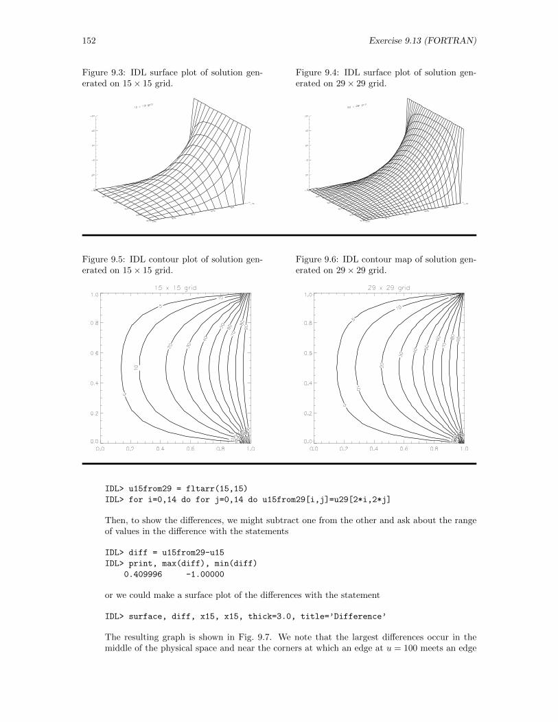
152 Exercise 9.13 (FORTRAN)
Figure 9.3: IDL surface plot of solution gen-erated on 15× 15 grid.
Figure 9.4: IDL surface plot of solution gen-erated on 29× 29 grid.
Figure 9.5: IDL contour plot of solution gen-erated on 15× 15 grid.
Figure 9.6: IDL contour map of solution gen-erated on 29× 29 grid.
IDL> u15from29 = fltarr(15,15)
IDL> for i=0,14 do for j=0,14 do u15from29[i,j]=u29[2*i,2*j]
Then, to show the differences, we might subtract one from the other and ask about the rangeof values in the difference with the statements
IDL> diff = u15from29-u15
IDL> print, max(diff), min(diff)
0.409996 -1.00000
or we could make a surface plot of the differences with the statement
IDL> surface, diff, x15, x15, thick=3.0, title=’Difference’
The resulting graph is shown in Fig. 9.7. We note that the largest differences occur in themiddle of the physical space and near the corners at which an edge at u = 100 meets an edge
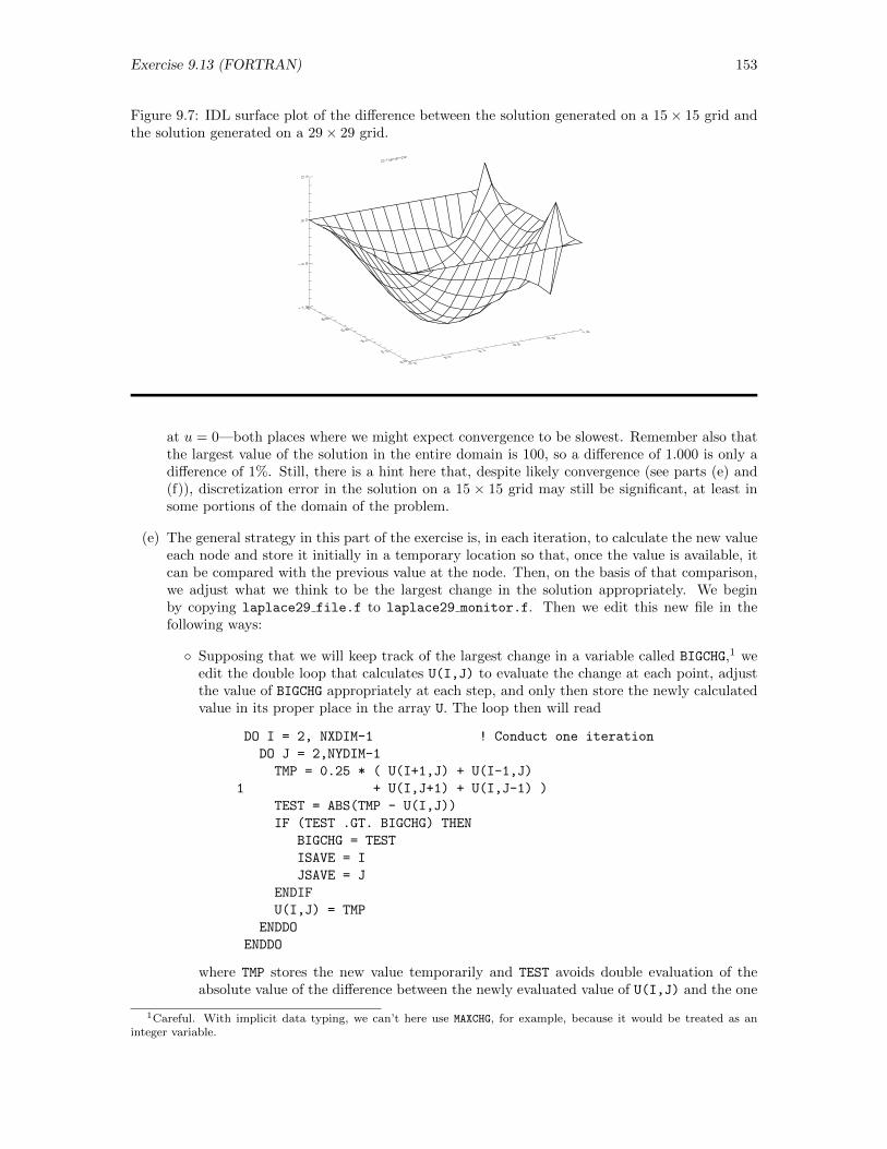
Exercise 9.13 (FORTRAN) 153
Figure 9.7: IDL surface plot of the difference between the solution generated on a 15× 15 grid andthe solution generated on a 29× 29 grid.
at u = 0—both places where we might expect convergence to be slowest. Remember also thatthe largest value of the solution in the entire domain is 100, so a difference of 1.000 is only adifference of 1%. Still, there is a hint here that, despite likely convergence (see parts (e) and(f)), discretization error in the solution on a 15 × 15 grid may still be significant, at least insome portions of the domain of the problem.
(e) The general strategy in this part of the exercise is, in each iteration, to calculate the new valueeach node and store it initially in a temporary location so that, once the value is available, itcan be compared with the previous value at the node. Then, on the basis of that comparison,we adjust what we think to be the largest change in the solution appropriately. We beginby copying laplace29 file.f to laplace29 monitor.f. Then we edit this new file in thefollowing ways:
Supposing that we will keep track of the largest change in a variable called BIGCHG,1 weedit the double loop that calculates U(I,J) to evaluate the change at each point, adjustthe value of BIGCHG appropriately at each step, and only then store the newly calculatedvalue in its proper place in the array U. The loop then will read
DO I = 2, NXDIM-1 ! Conduct one iteration
DO J = 2,NYDIM-1
TMP = 0.25 * ( U(I+1,J) + U(I-1,J)
1 + U(I,J+1) + U(I,J-1) )
TEST = ABS(TMP - U(I,J))
IF (TEST .GT. BIGCHG) THEN
BIGCHG = TEST
ISAVE = I
JSAVE = J
ENDIF
U(I,J) = TMP
ENDDO
ENDDO
where TMP stores the new value temporarily and TEST avoids double evaluation of theabsolute value of the difference between the newly evaluated value of U(I,J) and the one
1Careful. With implicit data typing, we can’t here use MAXCHG, for example, because it would be treated as aninteger variable.
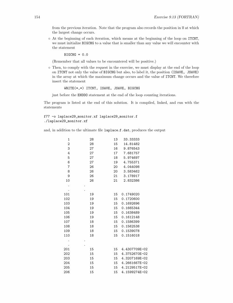
154 Exercise 9.13 (FORTRAN)
from the previous iteration. Note that the program also records the position in U at whichthe largest change occurs.
At the beginning of each iteration, which means at the beginning of the loop on ITCNT,we must initialize BIGCHG to a value that is smaller than any value we will encounter withthe statement
BIGCHG = 0.0
(Remember that all values to be encountered will be positive.)
Then, to comply with the request in the exercise, we must display at the end of the loopon ITCNT not only the value of BIGCHG but also, to label it, the position (ISAVE, JSAVE)
in the array at which the maximum change occurs and the value of ITCNT. We thereforeinsert the statement
WRITE(*,*) ITCNT, ISAVE, JSAVE, BIGCHG
just before the ENDDO statement at the end of the loop counting iterations.
The program is listed at the end of this solution. It is compiled, linked, and run with thestatements
f77 -o laplace29_monitor.xf laplace29_monitor.f
./laplace29_monitor.xf
and, in addition to the ultimate file laplace f.dat, produces the output
1 28 13 33.33333
2 28 15 14.81482
3 27 16 9.876543
4 27 17 7.681757
5 27 18 5.974697
6 27 19 4.755371
7 26 20 4.044098
8 26 20 3.583462
9 26 21 3.178917
10 26 21 2.832386
. .
. .
101 19 15 0.1749020
102 19 15 0.1720600
103 19 15 0.1692696
104 19 15 0.1665344
105 19 15 0.1638489
106 19 15 0.1612148
107 18 15 0.1586399
108 18 15 0.1562538
109 18 15 0.1539078
110 18 15 0.1516018
. .
. .
201 15 15 4.4307709E-02
202 15 15 4.3752670E-02
203 15 15 4.3207169E-02
204 15 15 4.2661667E-02
205 15 15 4.2129517E-02
206 15 15 4.1599274E-02
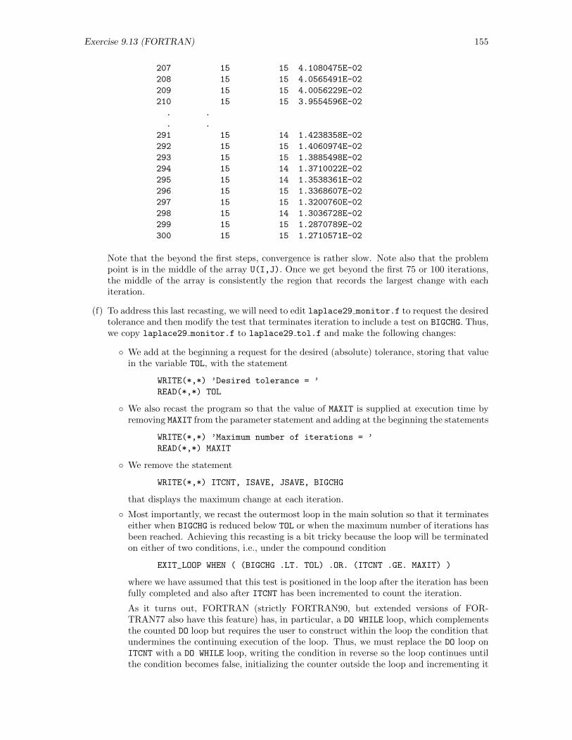
Exercise 9.13 (FORTRAN) 155
207 15 15 4.1080475E-02
208 15 15 4.0565491E-02
209 15 15 4.0056229E-02
210 15 15 3.9554596E-02
. .
. .
291 15 14 1.4238358E-02
292 15 15 1.4060974E-02
293 15 15 1.3885498E-02
294 15 14 1.3710022E-02
295 15 14 1.3538361E-02
296 15 15 1.3368607E-02
297 15 15 1.3200760E-02
298 15 14 1.3036728E-02
299 15 15 1.2870789E-02
300 15 15 1.2710571E-02
Note that the beyond the first steps, convergence is rather slow. Note also that the problempoint is in the middle of the array U(I,J). Once we get beyond the first 75 or 100 iterations,the middle of the array is consistently the region that records the largest change with eachiteration.
(f) To address this last recasting, we will need to edit laplace29 monitor.f to request the desiredtolerance and then modify the test that terminates iteration to include a test on BIGCHG. Thus,we copy laplace29 monitor.f to laplace29 tol.f and make the following changes:
We add at the beginning a request for the desired (absolute) tolerance, storing that valuein the variable TOL, with the statement
WRITE(*,*) ’Desired tolerance = ’
READ(*,*) TOL
We also recast the program so that the value of MAXIT is supplied at execution time byremoving MAXIT from the parameter statement and adding at the beginning the statements
WRITE(*,*) ’Maximum number of iterations = ’
READ(*,*) MAXIT
We remove the statement
WRITE(*,*) ITCNT, ISAVE, JSAVE, BIGCHG
that displays the maximum change at each iteration.
Most importantly, we recast the outermost loop in the main solution so that it terminateseither when BIGCHG is reduced below TOL or when the maximum number of iterations hasbeen reached. Achieving this recasting is a bit tricky because the loop will be terminatedon either of two conditions, i.e., under the compound condition
EXIT_LOOP WHEN ( (BIGCHG .LT. TOL) .OR. (ITCNT .GE. MAXIT) )
where we have assumed that this test is positioned in the loop after the iteration has beenfully completed and also after ITCNT has been incremented to count the iteration.
As it turns out, FORTRAN (strictly FORTRAN90, but extended versions of FOR-TRAN77 also have this feature) has, in particular, a DO WHILE loop, which complementsthe counted DO loop but requires the user to construct within the loop the condition thatundermines the continuing execution of the loop. Thus, we must replace the DO loop onITCNT with a DO WHILE loop, writing the condition in reverse so the loop continues untilthe condition becomes false, initializing the counter outside the loop and incrementing it
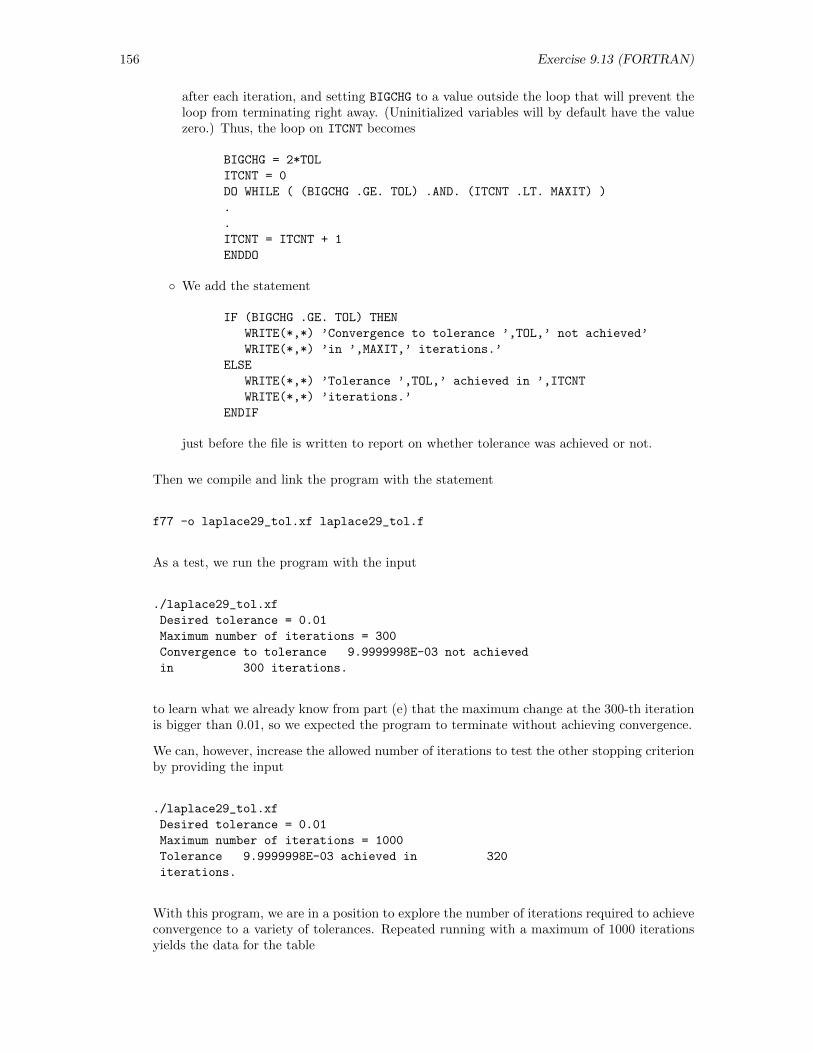
156 Exercise 9.13 (FORTRAN)
after each iteration, and setting BIGCHG to a value outside the loop that will prevent theloop from terminating right away. (Uninitialized variables will by default have the valuezero.) Thus, the loop on ITCNT becomes
BIGCHG = 2*TOL
ITCNT = 0
DO WHILE ( (BIGCHG .GE. TOL) .AND. (ITCNT .LT. MAXIT) )
.
.
ITCNT = ITCNT + 1
ENDDO
We add the statement
IF (BIGCHG .GE. TOL) THEN
WRITE(*,*) ’Convergence to tolerance ’,TOL,’ not achieved’
WRITE(*,*) ’in ’,MAXIT,’ iterations.’
ELSE
WRITE(*,*) ’Tolerance ’,TOL,’ achieved in ’,ITCNT
WRITE(*,*) ’iterations.’
ENDIF
just before the file is written to report on whether tolerance was achieved or not.
Then we compile and link the program with the statement
f77 -o laplace29_tol.xf laplace29_tol.f
As a test, we run the program with the input
./laplace29_tol.xf
Desired tolerance = 0.01
Maximum number of iterations = 300
Convergence to tolerance 9.9999998E-03 not achieved
in 300 iterations.
to learn what we already know from part (e) that the maximum change at the 300-th iterationis bigger than 0.01, so we expected the program to terminate without achieving convergence.
We can, however, increase the allowed number of iterations to test the other stopping criterionby providing the input
./laplace29_tol.xf
Desired tolerance = 0.01
Maximum number of iterations = 1000
Tolerance 9.9999998E-03 achieved in 320
iterations.
With this program, we are in a position to explore the number of iterations required to achieveconvergence to a variety of tolerances. Repeated running with a maximum of 1000 iterationsyields the data for the table
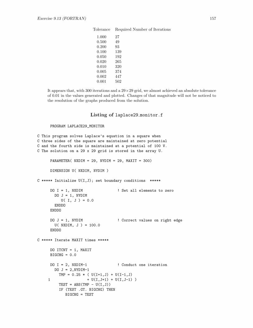
Exercise 9.13 (FORTRAN) 157
Tolerance Required Number of Iterations
1.000 270.500 490.200 930.100 1390.050 1920.020 2650.010 3200.005 3740.002 4470.001 502
It appears that, with 300 iterations and a 29×29 grid, we almost achieved an absolute toleranceof 0.01 in the values generated and plotted. Changes of that magnitude will not be noticed tothe resolution of the graphs produced from the solution.
Listing of laplace29 monitor.f
PROGRAM LAPLACE29_MONITOR
C This program solves Laplace’s equation in a square when
C three sides of the square are maintained at zero potential
C and the fourth side is maintained at a potential of 100 V.
C The solution on a 29 x 29 grid is stored in the array U.
PARAMETER( NXDIM = 29, NYDIM = 29, MAXIT = 300)
DIMENSION U( NXDIM, NYDIM )
C ***** Initialize U(I,J); set boundary conditions *****
DO I = 1, NXDIM ! Set all elements to zero
DO J = 1, NYDIM
U( I, J ) = 0.0
ENDDO
ENDDO
DO J = 1, NYDIM ! Correct values on right edge
U( NXDIM, J ) = 100.0
ENDDO
C ***** Iterate MAXIT times *****
DO ITCNT = 1, MAXIT
BIGCHG = 0.0
DO I = 2, NXDIM-1 ! Conduct one iteration
DO J = 2,NYDIM-1
TMP = 0.25 * ( U(I+1,J) + U(I-1,J)
1 + U(I,J+1) + U(I,J-1) )
TEST = ABS(TMP - U(I,J))
IF (TEST .GT. BIGCHG) THEN
BIGCHG = TEST
158 Exercise 9.13 (FORTRAN)
ISAVE = I
JSAVE = J
ENDIF
U(I,J) = TMP
ENDDO
ENDDO
WRITE(*,*) ITCNT, ISAVE, JSAVE, BIGCHG
ENDDO
C ***** Display solution *****
OPEN( UNIT = 1, FILE = ’laplace_f.dat’, STATUS = ’NEW’ )
DO J = 1, NYDIM
WRITE( UNIT = 1, FMT = 200 ) ( U(I,J), I=1,NXDIM )
ENDDO
CLOSE( UNIT = 1 )
200 FORMAT(’ ’, 29F7.2 )
END
Listing of laplace29 tol.f
PROGRAM LAPLACE29_TOL
C This program solves Laplace’s equation in a square when
C three sides of the square are maintained at zero potential
C and the fourth side is maintained at a potential of 100 V.
C The solution on a 29 x 29 grid is stored in the array U.
PARAMETER( NXDIM = 29, NYDIM = 29)
DIMENSION U( NXDIM, NYDIM )
WRITE(*,*) ’Desired tolerance = ’
READ(*,*) TOL
WRITE(*,*) ’Maximum number of iterations = ’
READ(*,*) MAXIT
C ***** Initialize U(I,J); set boundary conditions *****
DO I = 1, NXDIM ! Set all elements to zero
DO J = 1, NYDIM
U( I, J ) = 0.0
ENDDO
ENDDO
DO J = 1, NYDIM ! Correct values on right edge
U( NXDIM, J ) = 100.0
Exercise 9.13 (FORTRAN) 159
ENDDO
C ***** Iterate MAXIT times *****
BIGCHG = 2*TOL
ITCNT = 0
DO WHILE ( (BIGCHG .GE. TOL) .AND. (ITCNT .LT. MAXIT) )
BIGCHG = 0.0
DO I = 2, NXDIM-1 ! Conduct one iteration
DO J = 2,NYDIM-1
TMP = 0.25 * ( U(I+1,J) + U(I-1,J)
1 + U(I,J+1) + U(I,J-1) )
TEST = ABS(TMP - U(I,J))
IF (TEST .GT. BIGCHG) THEN
BIGCHG = TEST
ISAVE = I
JSAVE = J
ENDIF
U(I,J) = TMP
ENDDO
ENDDO
ITCNT = ITCNT + 1
ENDDO
IF (BIGCHG .GE. TOL) THEN
WRITE(*,*) ’Convergence to tolerance ’,TOL,’ not achieved’
WRITE(*,*) ’in ’,MAXIT,’ iterations.’
ELSE
WRITE(*,*) ’Tolerance ’,TOL,’ achieved in ’,ITCNT
WRITE(*,*) ’iterations.’
ENDIF
C ***** Display solution *****
OPEN( UNIT = 1, FILE = ’laplace_f.dat’, STATUS = ’NEW’ )
DO J = 1, NYDIM
WRITE( UNIT = 1, FMT = 200 ) ( U(I,J), I=1,NXDIM )
ENDDO
CLOSE( UNIT = 1 )
200 FORMAT(’ ’, 29F7.2 )
END
160 Exercise 9.16 (FORTRAN)
9.16 Exploring Trajectories in 3D (FORTRAN)
Exercise: The trajectory of a particle in three-dimensional space is given parametrically as afunction of time t by the position vector
r = x(t) i + y(t) j + z(t) k
You desire to fathom out the general character of this trajectory by using a graphical visualizationtool that does not have much computational capability. Thus, you must generate the data usingone tool but will visualize the trajectory with another tool. You elect to use an ASCII file tocommunicate the data from the first tool to the second. Suppose that the ASCII file produced bythe first tool is to be structured as follows:
• five lines of text describing the contents of the file and its origin,• one line containing the number of points N on the trajectory included in the file, and• N lines, each of which contains four floating point values separated by commas, those values
being in order t, x(t), y(t), and z(t) for a point on the trajectory. (The N lines are ordered byincreasing value of t.)
Describe a general procedure to create this file and then implement that procedure in at least onelanguage of your choice, testing your program(s) with the trajectory given by
r = cos t i + sin t j + 0.1t k
which describes the path followed by a charged particle in a constant magnetic field along the z axis.
Solution: In broad outline, the task we need to perform in solving this exercise is to initializeseveral variables and then, time instant by time instant, systematically move from the starting timethrough the desired number of steps, writing the results at each step to the desired file. Somewhereprior to the loop in which the coordinates are evaluated at each step, we would have to open theintended file and write the desired labeling lines to the file, and then after the loop we would haveto close the file. In outline (and in pseudocode), the program might have the general structure2
ATTACH NEW FILE filename ON CHANNEL 1
WRITE TO CHANNEL 1%, "Descriptive line 1"
WRITE TO CHANNEL 1%, "Descriptive line 2"
WRITE TO CHANNEL 1%, "Descriptive line 3"
WRITE TO CHANNEL 1%, "Descriptive line 4"
WRITE TO CHANNEL 1%, "Descriptive line 5"
nsteps% <-- ?? ! Set number of time steps
WRITE TO CHANNEL 1%, nsteps%+1% ! Write number of lines to file
tstart <-- ?? ! Set starting time
dt <-- ?? ! Set time increment between steps
ncnt% <-- 0 ! Initialize step counter
LOOP
t = tstart + dt*float(ncnt%) ! Set current time (tstart on first pass)
x <-- x(t) ! Evaluate x, y, z at current time
y <-- y(t)
z <-- z(t)
WRITE TO CHANNEL 1%, t, x, y, z ! Output values to file
EXIT_LOOP WHEN ncnt% = nsteps%
ncnt% <-- ncnt% + 1% ! Increment counter for next step
END_LOOP
CLOSE FILE ON CHANNEL 1%
2The function float used at the end of the loop forces a conversion of the integer ncnt% to floating point form forthe floating-point computation in which it appears.
Exercise 9.16 (FORTRAN) 161
Note the position at which ncnt% is incremented. Further, to minimize problems from cumulativeroundoff, note that the program calculates each new time by adding the appropriate multiple of dtto tstart rather than simply adding dt repeatedly to t. Since we are writing the values to the fileas they are generated, we have in the context of this program no reason to introduce a dimensionedarray to store all the values; we can afford to forget each value after it has been written to the file.
While conceptually fairly straightforward, the above program makes use of a loop structure thatis not available in FORTRAN. Before developing more explicit coding, we must recast the loop sothat the EXIT_LOOP statement appears at the beginning of the loop. To do so, we must “prime” theloop, i.e., we must execute the statements in the above loop but preceding the EXIT LOOP statementbefore entering the loop and then execute them again at the end of the loop. To prime the loop, theprogram above must be embellished to become
ATTACH NEW FILE filename ON CHANNEL 1%
WRITE TO CHANNEL 1%, "Descriptive line 1"
WRITE TO CHANNEL 1%, "Descriptive line 2"
WRITE TO CHANNEL 1%, "Descriptive line 3"
WRITE TO CHANNEL 1%, "Descriptive line 4"
WRITE TO CHANNEL 1%, "Descriptive line 5"
nsteps% <-- ?? ! Set number of time steps to take
WRITE TO CHANNEL 1%, nsteps%+1% ! Write number of lines to file
tstart <-- ?? ! Set starting time
dt <-- ?? ! Set time increment between steps
ncnt% <-- 0 ! Initialize step counter
t = tstart ! Initialize current time
x <-- x(t) ! Evaluate x, y, z at current time
y <-- y(t)
z <-- z(t)
WRITE TO CHANNEL 1%, t, x, y, z ! Output initial values to file
LOOP
EXIT_LOOP WHEN ncnt% = nsteps%
ncnt% <-- ncnt% + 1% ! Count step about to be taken
t = tstart + dt*float(ncnt%) ! Set current time
x <-- x(t) ! Evaluate x, y, z at current time
y <-- y(t)
z <-- z(t)
WRITE TO CHANNEL 1%, t, x, y, z ! Output current values to file
END_LOOP
CLOSE FILE ON CHANNEL 1%
Now, we are ready to recast this program into an explicit program in FORTRAN, though to createa compilable and runnable program, we must assume a specific trajectory, which we take to be thetrajectory defined by the parametric equations
x(t) = cos t ; y(t) = sin t ; z(t) = 0.1t (9.1)
Further, to facilitate exploration, we cast the actual program so that (1) the time step and thenumber of steps to be taken will be entered at execution time and (2) the descriptive lines reflectthe specific trajectory adopted as the example.3 We thus arrive at the program
3Note that a WRITE statement with no specified output will generate a blank line in the file.
162 Exercise 9.16 (FORTRAN)
PROGRAM TRAJECTORY
C ***** Open file, set number of steps, and write descriptive
C lines to file *****
OPEN( UNIT = 1, FILE = ’trajectory_f.dat’, STATUS = ’NEW’ )
WRITE( UNIT=1, FMT=* ) "Trajectory when "
WRITE( UNIT=1, FMT=* ) " x(t) = cos(t)"
WRITE( UNIT=1, FMT=* ) " y(t) = sin(t)"
WRITE( UNIT=1, FMT=* ) " z(t) = 0.1 t"
WRITE( UNIT=1, FMT=* )
WRITE( *,*) "Enter number of steps: " ! Set number of time steps to take
READ(*,*) NSTEPS
WRITE( UNIT=1, FMT=’(1X,I8)’ ) NSTEPS+1 ! Write number of lines to file
C ***** Initialize variables, prime loop, write initial values to file *****
TSTART = 0.0 ! Set starting time
WRITE( *,* ) "Enter time between points: " ! Set time increment between steps
READ( *, * ) DT
NCNT = 0 ! Initialize step counter
T = TSTART ! Initialize current time
X = COS(T) ! Evaluate x, y, z at current time
Y = SIN(T)
Z = 0.1*T
WRITE( UNIT=1, FMT=’(1X,4E15.5)’ ) T, X, Y, Z
! Output initial values to file
C ***** Evaluate desired number of steps, writing values at each step
C to file *****
DO NCNT = 1, NSTEPS
T = TSTART + DT*FLOAT(NCNT) ! Set current time
X = COS(T) ! Evaluate x, y, z at current time
Y = SIN(T)
Z = 0.1*T
WRITE( UNIT=1, FMT=’(1X,4E15.5)’ ) T, X, Y, Z
! Output current values to file
ENDDO
C ***** Close file *****
CLOSE( UNIT=1 )
END
This program would be compiled and executed with the statements
f77 -o trajectory.xf trajectory.f
./trajectory.xf
When run, with the input4
4The actual entered values will be on lines by themselves; we here compress the display by placing the entered
Exercise 9.16 (FORTRAN) 163
Enter number of steps: 10
Enter time between points:0.1
the resulting file trajectory f.dat contains the lines
Trajectory when
x(t) = cos(t)
y(t) = sin(t)
z(t) = 0.1 t
11
0.00000E+00 0.10000E+01 0.00000E+00 0.00000E+00
0.10000E+00 0.99500E+00 0.99833E-01 0.10000E-01
0.20000E+00 0.98007E+00 0.19867E+00 0.20000E-01
0.30000E+00 0.95534E+00 0.29552E+00 0.30000E-01
0.40000E+00 0.92106E+00 0.38942E+00 0.40000E-01
0.50000E+00 0.87758E+00 0.47943E+00 0.50000E-01
0.60000E+00 0.82534E+00 0.56464E+00 0.60000E-01
0.70000E+00 0.76484E+00 0.64422E+00 0.70000E-01
0.80000E+00 0.69671E+00 0.71736E+00 0.80000E-01
0.90000E+00 0.62161E+00 0.78333E+00 0.90000E-01
0.10000E+01 0.54030E+00 0.84147E+00 0.10000E+00
To produce the desired graphical display of this trajectory, we need to input this file into asuitable graphics program. In IDL, we would execute the statements
ln = "" ; Set string variable for reading lines
openr, 1, ’trajectory_f.dat’ ; Open file
for i=1,5 do readf, 1, ln ; Read past and ignore first 5 lines
readf, 1, nlines ; Read number of lines
traj = fltarr(4,nlines) ; Dimension array for data
readf, 1, traj ; Read data
close, 1 ; Close the file
t = traj[0,*] & x = traj[1,*] & y = traj[2,*] & z = traj[3,*]
to open the file, read past the descriptive lines, read the data contained in the file, close the file, and(for convenience in reference) extract each column into a more mnemonically named variable. Then,to display the trajectory in a graph, we execute the statements (see Section 2.16.2 of CPSUP)
scale3, xrange=[-1.0,1.0], yrange=[-1.0,1.0], zrange=[0.0,0.1]
plots, x, y, z, /t3d
The scaling was determined by noting that −1.0 ≤ x, y ≤ 1.0 (since those are the limits on the sineand cosine functions) and 0 ≤ z ≤ 0.1.
The sample above, of course, did not trace the trajectory very far away from its origin. To finda more suitable total time interval, we note that x and y each take time 2π to complete one cycle. Ifwe want to plot the trajectory through, say, 4 full cycles, we should allow t to run from 0 to about8π ≈ 25.0, whence z will run from 0 to 2.5. If we rerun the program with the input
Enter number of steps: 250
Enter time between points: 0.1
values on the same line as the associated prompt.
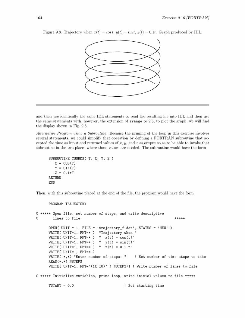
164 Exercise 9.16 (FORTRAN)
Figure 9.8: Trajectory when x(t) = cos t, y(t) = sin t, z(t) = 0.1t. Graph produced by IDL.
and then use identically the same IDL statements to read the resulting file into IDL and then usethe same statements with, however, the extension of zrange to 2.5, to plot the graph, we will findthe display shown in Fig. 9.8.
Alternative Program using a Subroutine: Because the priming of the loop in this exercise involvesseveral statements, we could simplify that operation by defining a FORTRAN subroutine that ac-cepted the time as input and returned values of x, y, and z as output so as to be able to invoke thatsubroutine in the two places where those values are needed. The subroutine would have the form
SUBROUTINE COORDS( T, X, Y, Z )
X = COS(T)
Y = SIN(T)
Z = 0.1*T
RETURN
END
Then, with this subroutine placed at the end of the file, the program would have the form
PROGRAM TRAJECTORY
C ***** Open file, set number of steps, and write descriptive
C lines to file *****
OPEN( UNIT = 1, FILE = ’trajectory_f.dat’, STATUS = ’NEW’ )
WRITE( UNIT=1, FMT=* ) "Trajectory when "
WRITE( UNIT=1, FMT=* ) " x(t) = cos(t)"
WRITE( UNIT=1, FMT=* ) " y(t) = sin(t)"
WRITE( UNIT=1, FMT=* ) " z(t) = 0.1 t"
WRITE( UNIT=1, FMT=* )
WRITE( *,*) "Enter number of steps: " ! Set number of time steps to take
READ(*,*) NSTEPS
WRITE( UNIT=1, FMT=’(1X,I8)’ ) NSTEPS+1 ! Write number of lines to file
C ***** Initialize variables, prime loop, write initial values to file *****
TSTART = 0.0 ! Set starting time
Exercise 9.16 (FORTRAN) 165
WRITE( *,* ) "Enter time between points: " ! Set time increment between steps
READ( *, * ) DT
NCNT = 0 ! Initialize step counter
T = TSTART ! Initialize current time
CALL COORDS( T, X, Y, Z ) ! Initialize X, Y, Z
WRITE( UNIT=1, FMT=’(1X,4E15.5)’ ) T, X, Y, Z
! Output initial values to file
C ***** Evaluate desired number of steps, writing values at each step
C to file *****
DO NCNT = 1, NSTEPS
T = TSTART + DT*FLOAT(NCNT) ! Set current time
CALL COORDS( T, X, Y, Z ) ! Evaluate x, y, z at current time
WRITE( UNIT=1, FMT=’(1X,4E15.5)’ ) T, X, Y, Z
! Output current values to file
ENDDO
C ***** Close file *****
CLOSE( UNIT=1 )
END
SUBROUTINE COORDS( T, X, Y, Z )
X = COS(T)
Y = SIN(T)
Z = 0.1*T
RETURN
END
166 Exercise 9.22 (FORTRAN)
9.22 Great Circle Distances (FORTRAN)
Exercise: Write and test a program to ask for the latitude and longitude of both a point ofdeparture D and a point of arrival A on the surface of the earth and then calculate and print outthe “crow-flies” distance along a great circle route from D to A. Make sure your program prints theshorter of the two distances, regardless of the location of the points, and make sure your programdoesn’t run into difficulties if the two points happen to be at opposite ends of a diameter. Take theearth to be a perfect sphere with a circumference of 24900 miles (radius 3963 miles). For purposesof testing, note that Albany, NY, is at [4340′ N, 7345′ W]; Grand Junction, CO, is at [395′ N,10833′ W]; Los Angeles, CA, is at [343′ N, 11815′ W]; Appleton, WI, is at [4416′ N, 8825′ W];Calcutta India, is at [2232′ N, 8820′ E]; Sydney, Australia, is at [3352′ S, 15112′ E]; Paris,France, is at [4849′ N, 229′ E]; and Stockholm, Sweden, is at [5921′ N, 184′ E].
Solution: Introduce a coordinate system in which the axis of the earth defines the z axis, a linefrom the center of the earth to the equator at a point at longitude of 0 defines the x axis, and a linefrom the center of the earth to the equation at a point at longitude 90 E. In that system, let thepolar and azimuthal angles (not the latitude and longitude) of one point be θ1, φ1 and the polar andazimuthal angles of the other point be θ2, φ2, where 0 ≤ θ1, θ2 ≤ 90 and −180 ≤ φ1, φ2 ≤ 180.Further, let the radius of the earth, considered to be a sphere, be R. Then vector r1 and r2 fromthe center of the earth to each of these points are given by
r1 = R(sin θ1 cosφ1 i + sin θ1 sinφ1 j + cos θ1 k
)and
r2 = R(sin θ2 cosφ2 i + sin θ2 sinφ2 j + cos θ2 k
)Remembering that the dot product of two vectors A and B is defined by
A •B = |A| |B| cos θAB =⇒ cos θAB =A •B|A| |B|
we conclude that the angle subtended at the center of the earth by the two vectors identifying thepoints of interest on the earth’s surface is given by
θ12 = cos−1
(r1 • r2
r1 r2
)=
r1
R• r2
R
and then that the required distance is given by
d = Rθ12
A listing of a program to accomplish the desired task is presented at the end of this solution. Thetask is complicated a bit because the input information is to be given in terms of the normal latitude-longitude designation of the points of interest, e.g., Albany, NY, at 42 40′ N latitude, 73 45′ Wlongitude. Thus, the first task of the program before calculating the distance between two pointsso specified is to obtain the input coordinates in the conventional terminology and then convertthat specification for each into the polar and azimuthal angles involved in the above expressionsfor the radius vectors of the two points. We will use implicit variable typing, except that we needto declare explicitly four character variables to contain single characters N or S for latitude, E orW longitude. Using S as the initial character of a variable pertaining to the starting point and E
as the initial character for the ending point, LAT and LON to convey latitude and longitude, andDEG and MIN in a variable name to convey degrees and minutes, we begin—Section 1—by declaringfour character variables that will ultimately contain the latitude and longitude of each point ofinterest and dimensioning two vectors that will ultimately contain the three components of the twovectors r1/R and r2/R. Then—Section 2—we set important constants. Next—Section 3—we printinstructions to clarify the way in which input data will be provided. In Section 4, we actually obtainthe input data, storing the three values for each latitude and longitude in three separate variables.
Exercise 9.22 (FORTRAN) 167
The actual calculation begins in Section 5, where each specification of a latitude or longitudeis converted into the corresponding polar or azimuthal angle in the standard coordinate system andultimately expressed in radians. Note that, for south latitudes and west longitudes, the input anglemust have its sign changed and that the polar angles must be expressed as angles down from thenorth pole rather than up or down from the equator.
Once the angles have been converted into the conventional coordinate system, we can calculate—Section 6—the three components of the vectors r1/R and r2/R, storing them in the arrays preparedin Section 1, and then the angle of interest.
Finally—Section 7—we calculate and display the required distance.
After storing this program in a file named greatcircle.f in the default directory, we compilelink and run the program for sample input with the statements5
f77 -o greatcircle.xf greatcircle.f
./greatcircle.xf
Latitudes should be given as three entries
in, for example, the form 15,30,N for
15 degrees, 30 minutes north latitude.
Degrees will range from 0 to 90 and minutes
from 0 to 60; compass direction will be
either N or S. Entries should be separated
by commas.
Longitudes should also be given as three
entries in, for example, the form 89,44,W
for 89 degrees, 44 minutes west longitude.
Degrees will range from 0 to 180 and minutes
from 0 to 60; compass direction will be
either W or E. Entries should be separated
by commas.
Note that each triplet is entered using
commas but NO spaces to separate values.
Starting latitude: 0,0,N
Starting longitude: 0,0,E
Ending latitude: 0,0,N
Ending longitude: 90,0,E
The distance is 6225.00 miles.
As a test, we have specified two points that are on the equator and 90 apart, in which case thedistance should be one-quarter of the earth’s circumference (i.e., 24900/4 = 6225 miles), which theprogram has calculated as well. With a point at the pole and a second point on the equator, theresult is
Starting latitude: 90,0,N
Starting longitude: 0,0,E
Ending latitude: 0,0,N
Ending longitude: 0,0,E
The distance is 6225.00 miles.
5To save space here, input data are displayed on the same line as the prompting message. In the actual run, thesevalues will be typed on the line after the prompt.
168 Exercise 9.22 (FORTRAN)
We again confirm the expected value of one-quarter of the circumference of the earth. More in-terestingly, the distance between Albany, NY (latitude and longitude above) and Los Angeles, CA(34 3′ N, 118 15′ W) is
Starting latitude: 42,40,N
Starting longitude: 73,45,W
Ending latitude: 34,3,N
Ending longitude: 118,15,W
The distance is 2456.11 miles.
We make two further tests. For two points that are on the equator but more than 90 apart,say, 120 we find that
Starting latitude: 0,0,S
Starting longitude: 90,0,E
Ending latitude: 0,0,N
Ending longitude: 45,0,W
The distance is 9337.50 miles.
which is, as expected, three-eighths of the circumference of the earth ((3/8)×24900 = 9337.5 miles).For two points that are on the equator and 270 apart, we find that
Starting latitude: 0,0,S
Starting longitude: 90,0,E
Ending latitude: 0,0,N
Ending longitude: 180,0,W
The distance is 6225.00 miles.
which is correct (one-quarter the circumference of the earth).
These results appear to be correct. The remaining source of concern reflects the fact that theinverse cosine function has some ambiguities. For the correctness of the above analysis, we haveassumed that the inverse cosine returns an angle between zero and π (0 and 180). To check thatassumption, we write the quick program
PROGRAM TEST
DIMENSION ARCCOS(11), ANGLE(11)
PI = 3.14159265
DO I = 1,11
ARCCOS(I) = 0.2*FLOAT(I-6) ! Values from -1.0 to 1.0
ANGLE(I) = ACOS(ARCCOS(I)) ! Find inverse cosine
ANGLE(I) = 180.0*ANGLE(I)/PI ! Convert to degrees
WRITE(*,*) ARCCOS(I), ANGLE(I) ! Display results
ENDDO
END
Then we compile, link, and run this program with the statements
f77 -o test.xf test.f
./test.xf
Exercise 9.22 (FORTRAN) 169
-1. 180.
-0.800000012 143.130096
-0.600000024 126.869896
-0.400000006 113.578178
-0.200000003 101.536957
0. 90.
0.200000003 78.4630432
0.400000006 66.4218216
0.600000024 53.1301003
0.800000012 36.8698959
1. 0.
(The output in this display was rearranged a bit to align columns.) Evidently the FORTRAN inversecosine function does what we had expected. Thus, the program designed to address this exercisewill apparently work properly, always returning an angular separation of the two points of interestin the range from 0 to 180, i.e., the program will always return the shorter great circle distancebetween the two points even if the angle between the associated two vectors exceeds 180.
Final Program for Exercise 9.22
PROGRAM greatcircle
! *** 1. Declare those variables needing declaring
CHARACTER :: SLATDIR, SLONDIR, ELATDIR, ELONDIR
DIMENSION X1(3), X2(3)
! *** 2. Set constants ***
CIRCUM = 24900.0
PI = 3.1415926535
RADIUS = CIRCUM/(2.0*PI)
! *** 3. Provide instructions ***
WRITE(*,*)
WRITE(*, ’(1X,A)’) ’Latitudes should be given as three entries’
WRITE(*, ’(1X,A)’) ’in, for example, the form 15,30,N for’
WRITE(*, ’(1X,A)’) ’15 degrees, 30 minutes north latitude.’
WRITE(*, ’(1X,A)’) ’Degrees will range from 0 to 90 and minutes’
WRITE(*, ’(1X,A)’) ’from 0 to 60; compass direction will be’
WRITE(*, ’(1X,A)’) ’either N or S. Entries should be separated’
WRITE(*, ’(1X,A)’) ’by commas.’
WRITE(*,*)
WRITE(*, ’(1X,A)’) ’Longitudes should also be given as three’
WRITE(*, ’(1X,A)’) ’entries in, for example, the form 89,44,W’
WRITE(*, ’(1X,A)’) ’for 89 degrees, 44 minutes west longitude.’
WRITE(*, ’(1X,A)’) ’Degrees will range from 0 to 180 and minutes’
WRITE(*, ’(1X,A)’) ’from 0 to 60; compass direction will be ’
WRITE(*, ’(1X,A)’) ’either W or E. Entries should be separated’
WRITE(*, ’(1X,A)’) ’by commas.’
WRITE(*,*)
WRITE(*, ’(1X,A)’) ’Note that each triplet is entered using’
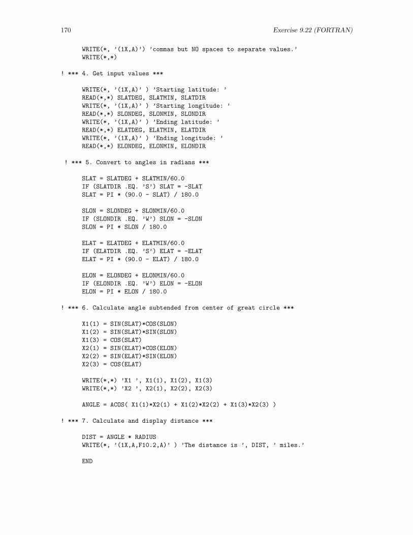
170 Exercise 9.22 (FORTRAN)
WRITE(*, ’(1X,A)’) ’commas but NO spaces to separate values.’
WRITE(*,*)
! *** 4. Get input values ***
WRITE(*, ’(1X,A)’ ) ’Starting latitude: ’
READ(*,*) SLATDEG, SLATMIN, SLATDIR
WRITE(*, ’(1X,A)’ ) ’Starting longitude: ’
READ(*,*) SLONDEG, SLONMIN, SLONDIR
WRITE(*, ’(1X,A)’ ) ’Ending latitude: ’
READ(*,*) ELATDEG, ELATMIN, ELATDIR
WRITE(*, ’(1X,A)’ ) ’Ending longitude: ’
READ(*,*) ELONDEG, ELONMIN, ELONDIR
! *** 5. Convert to angles in radians ***
SLAT = SLATDEG + SLATMIN/60.0
IF (SLATDIR .EQ. ’S’) SLAT = -SLAT
SLAT = PI * (90.0 - SLAT) / 180.0
SLON = SLONDEG + SLONMIN/60.0
IF (SLONDIR .EQ. ’W’) SLON = -SLON
SLON = PI * SLON / 180.0
ELAT = ELATDEG + ELATMIN/60.0
IF (ELATDIR .EQ. ’S’) ELAT = -ELAT
ELAT = PI * (90.0 - ELAT) / 180.0
ELON = ELONDEG + ELONMIN/60.0
IF (ELONDIR .EQ. ’W’) ELON = -ELON
ELON = PI * ELON / 180.0
! *** 6. Calculate angle subtended from center of great circle ***
X1(1) = SIN(SLAT)*COS(SLON)
X1(2) = SIN(SLAT)*SIN(SLON)
X1(3) = COS(SLAT)
X2(1) = SIN(ELAT)*COS(ELON)
X2(2) = SIN(ELAT)*SIN(ELON)
X2(3) = COS(ELAT)
WRITE(*,*) ’X1 ’, X1(1), X1(2), X1(3)
WRITE(*,*) ’X2 ’, X2(1), X2(2), X2(3)
ANGLE = ACOS( X1(1)*X2(1) + X1(2)*X2(2) + X1(3)*X2(3) )
! *** 7. Calculate and display distance ***
DIST = ANGLE * RADIUS
WRITE(*, ’(1X,A,F10.2,A)’ ) ’The distance is ’, DIST, ’ miles.’
END
Exercise 9.12 (C) 171
9.12 Conversion from Celsius to Fahrenheit (C)
Exercise: Write, compile, and test a program that asks for the input of a temperature inCelsius and prints out the corresponding temperature in Fahrenheit. To make it a bit more of achallenge, write the program in such a way that it asks repeatedly for Celsius temperatures untilthe temperature 9999 is entered, at which point the program terminates smoothly.
Solution: The conversion from a temperature C in Celsius to the corresponding temperatureF in Fahrenheit is given by the equation
F =9
5C + 32
At base, a C program to achieve this conversion must ask for the input of a Celsius temperaturewith statements like
printf( "\nEnter temperature in Celsius: ");
scanf( "%f", &C );
convert the value to Celsius by invoking the above equation with a statement like
F = 9.0*C/5.0 + 32.0
and then output the result with a statement like
printf( "Temperature in Fahrenheit = %10.2", F );
This exercise, however, asks that the conversion be placed in a loop such that the program asksrepeatedly for Celsius temperatures and effects the conversion of each, stopping only when theflagging value 9999 is entered in place of a legitimate Celsius temperature. To achieve that end withthe loop structures that are available in C, we must prime the loop with the entry of the first valueoutside of the loop. At that point, we will have available the first Celsius temperature for use inthe condition that determines whether the loop will be executed or not. Within the loop and afterthe temperature has been converted, we then must ask for the entry of the next Celsius temperature.That way, when the loop bounces back to the beginning and the controlling condition is tested, thatcondition will be able to detect the flag 9999 and terminate the loop when the time comes. Wemust, of course, also include whatever libraries are necessary and declare all variables appropriately.A complete program, including the loop and its control, might involve the statements
/* PROGRAM cent_to_fahr.c */
#include <stdio.h>
main()
float C, F; /* For temperatures */
printf( "\nEnter temperature in Celsius: ");
scanf( "%f", &C );
while (C != 9999)
F = 9.0*C/5.0 + 32.0;
printf( "Temperature in Fahrenheit = %10.2f", F );
printf( "\nEnter temperature in Celsius: ");
scanf( "%f", &C );
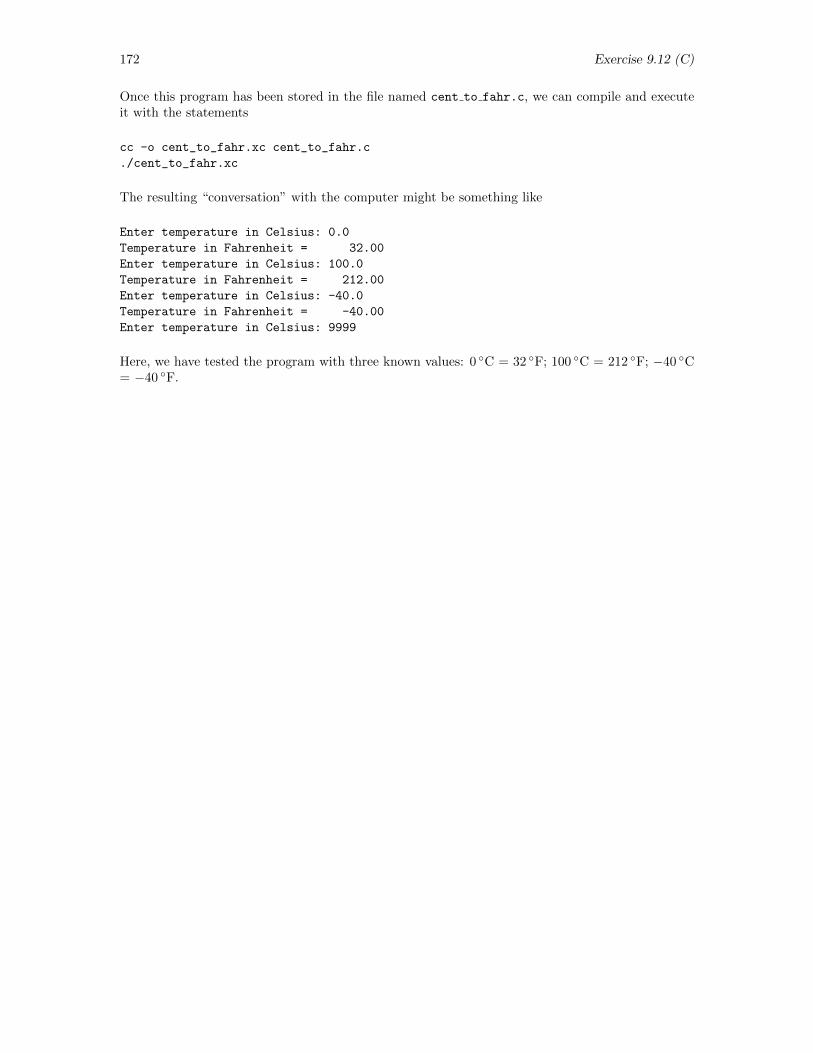
172 Exercise 9.12 (C)
Once this program has been stored in the file named cent to fahr.c, we can compile and executeit with the statements
cc -o cent_to_fahr.xc cent_to_fahr.c
./cent_to_fahr.xc
The resulting “conversation” with the computer might be something like
Enter temperature in Celsius: 0.0
Temperature in Fahrenheit = 32.00
Enter temperature in Celsius: 100.0
Temperature in Fahrenheit = 212.00
Enter temperature in Celsius: -40.0
Temperature in Fahrenheit = -40.00
Enter temperature in Celsius: 9999
Here, we have tested the program with three known values: 0 C = 32 F; 100 C = 212 F; −40 C= −40 F.
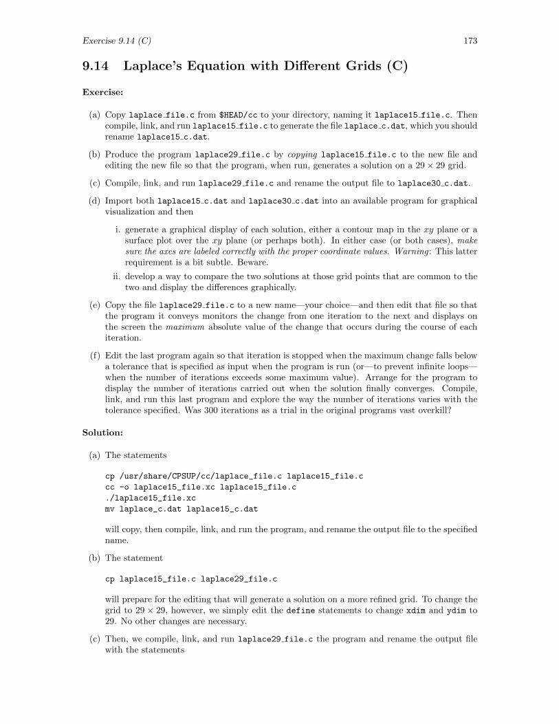
Exercise 9.14 (C) 173
9.14 Laplace’s Equation with Different Grids (C)
Exercise:
(a) Copy laplace file.c from $HEAD/cc to your directory, naming it laplace15 file.c. Thencompile, link, and run laplace15 file.c to generate the file laplace c.dat, which you shouldrename laplace15 c.dat.
(b) Produce the program laplace29 file.c by copying laplace15 file.c to the new file andediting the new file so that the program, when run, generates a solution on a 29× 29 grid.
(c) Compile, link, and run laplace29 file.c and rename the output file to laplace30 c.dat.
(d) Import both laplace15 c.dat and laplace30 c.dat into an available program for graphicalvisualization and then
i. generate a graphical display of each solution, either a contour map in the xy plane or asurface plot over the xy plane (or perhaps both). In either case (or both cases), makesure the axes are labeled correctly with the proper coordinate values. Warning : This latterrequirement is a bit subtle. Beware.
ii. develop a way to compare the two solutions at those grid points that are common to thetwo and display the differences graphically.
(e) Copy the file laplace29 file.c to a new name—your choice—and then edit that file so thatthe program it conveys monitors the change from one iteration to the next and displays onthe screen the maximum absolute value of the change that occurs during the course of eachiteration.
(f) Edit the last program again so that iteration is stopped when the maximum change falls belowa tolerance that is specified as input when the program is run (or—to prevent infinite loops—when the number of iterations exceeds some maximum value). Arrange for the program todisplay the number of iterations carried out when the solution finally converges. Compile,link, and run this last program and explore the way the number of iterations varies with thetolerance specified. Was 300 iterations as a trial in the original programs vast overkill?
Solution:
(a) The statements
cp /usr/share/CPSUP/cc/laplace_file.c laplace15_file.c
cc -o laplace15_file.xc laplace15_file.c
./laplace15_file.xc
mv laplace_c.dat laplace15_c.dat
will copy, then compile, link, and run the program, and rename the output file to the specifiedname.
(b) The statement
cp laplace15_file.c laplace29_file.c
will prepare for the editing that will generate a solution on a more refined grid. To change thegrid to 29 × 29, however, we simply edit the define statements to change xdim and ydim to29. No other changes are necessary.
(c) Then, we compile, link, and run laplace29 file.c the program and rename the output filewith the statements
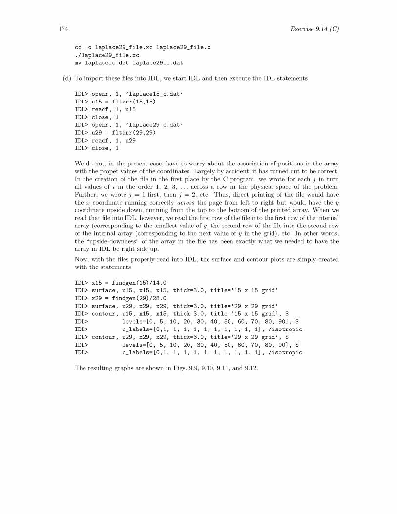
174 Exercise 9.14 (C)
cc -o laplace29_file.xc laplace29_file.c
./laplace29_file.xc
mv laplace_c.dat laplace29_c.dat
(d) To import these files into IDL, we start IDL and then execute the IDL statements
IDL> openr, 1, ’laplace15_c.dat’
IDL> u15 = fltarr(15,15)
IDL> readf, 1, u15
IDL> close, 1
IDL> openr, 1, ’laplace29_c.dat’
IDL> u29 = fltarr(29,29)
IDL> readf, 1, u29
IDL> close, 1
We do not, in the present case, have to worry about the association of positions in the arraywith the proper values of the coordinates. Largely by accident, it has turned out to be correct.In the creation of the file in the first place by the C program, we wrote for each j in turnall values of i in the order 1, 2, 3, . . . across a row in the physical space of the problem.Further, we wrote j = 1 first, then j = 2, etc. Thus, direct printing of the file would havethe x coordinate running correctly across the page from left to right but would have the ycoordinate upside down, running from the top to the bottom of the printed array. When weread that file into IDL, however, we read the first row of the file into the first row of the internalarray (corresponding to the smallest value of y, the second row of the file into the second rowof the internal array (corresponding to the next value of y in the grid), etc. In other words,the “upside-downness” of the array in the file has been exactly what we needed to have thearray in IDL be right side up.
Now, with the files properly read into IDL, the surface and contour plots are simply createdwith the statements
IDL> x15 = findgen(15)/14.0
IDL> surface, u15, x15, x15, thick=3.0, title=’15 x 15 grid’
IDL> x29 = findgen(29)/28.0
IDL> surface, u29, x29, x29, thick=3.0, title=’29 x 29 grid’
IDL> contour, u15, x15, x15, thick=3.0, title=’15 x 15 grid’, $
IDL> levels=[0, 5, 10, 20, 30, 40, 50, 60, 70, 80, 90], $
IDL> c_labels=[0,1, 1, 1, 1, 1, 1, 1, 1, 1, 1], /isotropic
IDL> contour, u29, x29, x29, thick=3.0, title=’29 x 29 grid’, $
IDL> levels=[0, 5, 10, 20, 30, 40, 50, 60, 70, 80, 90], $
IDL> c_labels=[0,1, 1, 1, 1, 1, 1, 1, 1, 1, 1], /isotropic
The resulting graphs are shown in Figs. 9.9, 9.10, 9.11, and 9.12.
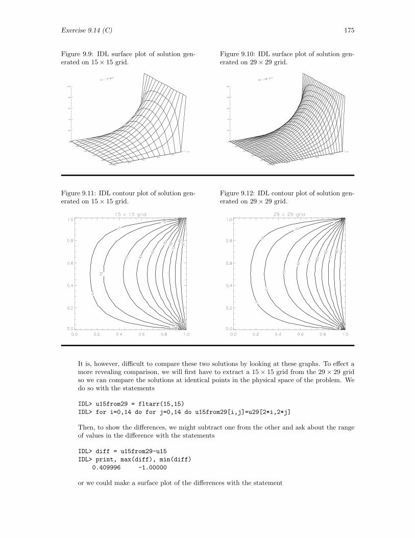
Exercise 9.14 (C) 175
Figure 9.9: IDL surface plot of solution gen-erated on 15× 15 grid.
Figure 9.10: IDL surface plot of solution gen-erated on 29× 29 grid.
Figure 9.11: IDL contour plot of solution gen-erated on 15× 15 grid.
Figure 9.12: IDL contour plot of solution gen-erated on 29× 29 grid.
It is, however, difficult to compare these two solutions by looking at these graphs. To effect amore revealing comparison, we will first have to extract a 15 × 15 grid from the 29 × 29 gridso we can compare the solutions at identical points in the physical space of the problem. Wedo so with the statements
IDL> u15from29 = fltarr(15,15)
IDL> for i=0,14 do for j=0,14 do u15from29[i,j]=u29[2*i,2*j]
Then, to show the differences, we might subtract one from the other and ask about the rangeof values in the difference with the statements
IDL> diff = u15from29-u15
IDL> print, max(diff), min(diff)
0.409996 -1.00000
or we could make a surface plot of the differences with the statement
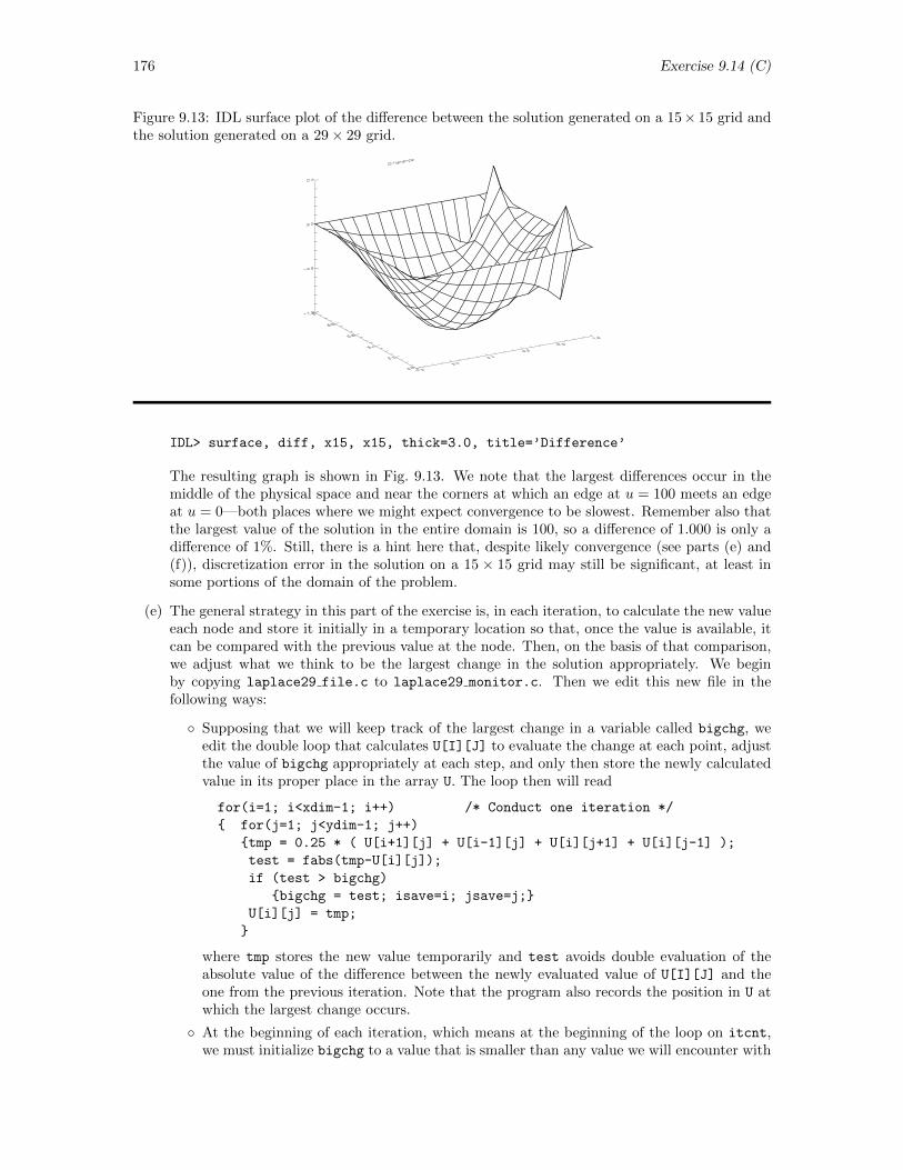
176 Exercise 9.14 (C)
Figure 9.13: IDL surface plot of the difference between the solution generated on a 15× 15 grid andthe solution generated on a 29× 29 grid.
IDL> surface, diff, x15, x15, thick=3.0, title=’Difference’
The resulting graph is shown in Fig. 9.13. We note that the largest differences occur in themiddle of the physical space and near the corners at which an edge at u = 100 meets an edgeat u = 0—both places where we might expect convergence to be slowest. Remember also thatthe largest value of the solution in the entire domain is 100, so a difference of 1.000 is only adifference of 1%. Still, there is a hint here that, despite likely convergence (see parts (e) and(f)), discretization error in the solution on a 15 × 15 grid may still be significant, at least insome portions of the domain of the problem.
(e) The general strategy in this part of the exercise is, in each iteration, to calculate the new valueeach node and store it initially in a temporary location so that, once the value is available, itcan be compared with the previous value at the node. Then, on the basis of that comparison,we adjust what we think to be the largest change in the solution appropriately. We beginby copying laplace29 file.c to laplace29 monitor.c. Then we edit this new file in thefollowing ways:
Supposing that we will keep track of the largest change in a variable called bigchg, weedit the double loop that calculates U[I][J] to evaluate the change at each point, adjustthe value of bigchg appropriately at each step, and only then store the newly calculatedvalue in its proper place in the array U. The loop then will read
for(i=1; i<xdim-1; i++) /* Conduct one iteration */
for(j=1; j<ydim-1; j++)
tmp = 0.25 * ( U[i+1][j] + U[i-1][j] + U[i][j+1] + U[i][j-1] );
test = fabs(tmp-U[i][j]);
if (test > bigchg)
bigchg = test; isave=i; jsave=j;
U[i][j] = tmp;
where tmp stores the new value temporarily and test avoids double evaluation of theabsolute value of the difference between the newly evaluated value of U[I][J] and theone from the previous iteration. Note that the program also records the position in U atwhich the largest change occurs.
At the beginning of each iteration, which means at the beginning of the loop on itcnt,we must initialize bigchg to a value that is smaller than any value we will encounter with
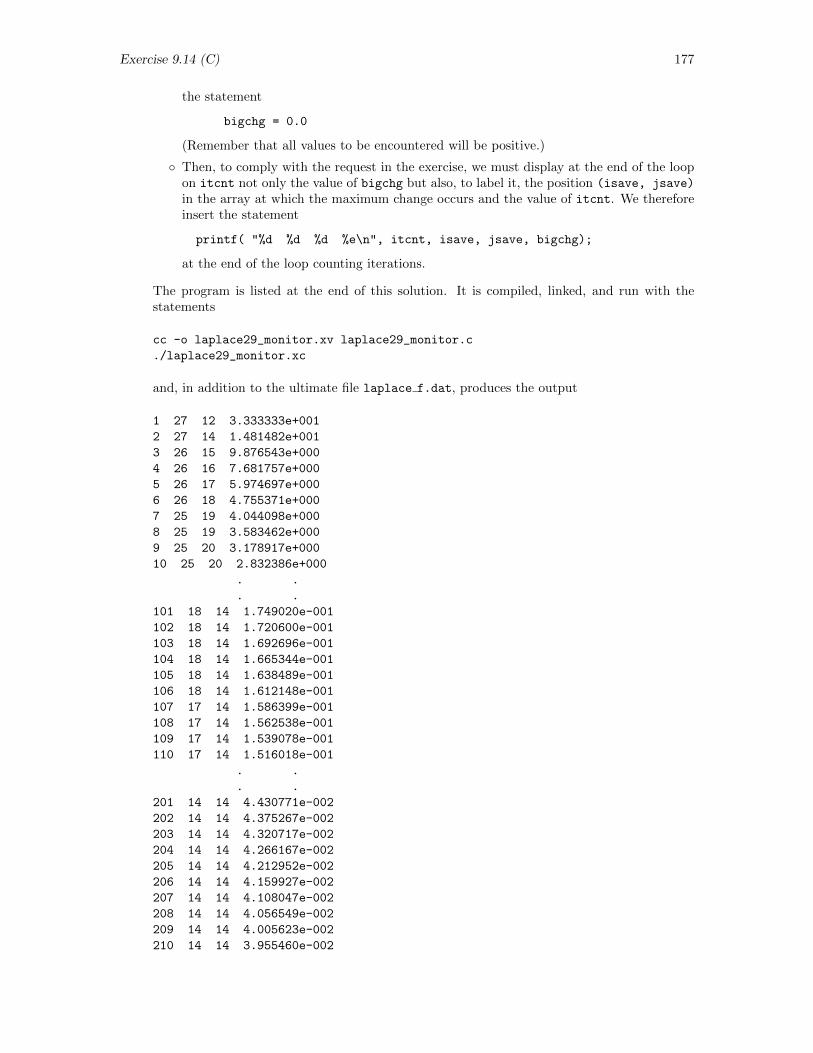
Exercise 9.14 (C) 177
the statement
bigchg = 0.0
(Remember that all values to be encountered will be positive.)
Then, to comply with the request in the exercise, we must display at the end of the loopon itcnt not only the value of bigchg but also, to label it, the position (isave, jsave)
in the array at which the maximum change occurs and the value of itcnt. We thereforeinsert the statement
printf( "%d %d %d %e\n", itcnt, isave, jsave, bigchg);
at the end of the loop counting iterations.
The program is listed at the end of this solution. It is compiled, linked, and run with thestatements
cc -o laplace29_monitor.xv laplace29_monitor.c
./laplace29_monitor.xc
and, in addition to the ultimate file laplace f.dat, produces the output
1 27 12 3.333333e+001
2 27 14 1.481482e+001
3 26 15 9.876543e+000
4 26 16 7.681757e+000
5 26 17 5.974697e+000
6 26 18 4.755371e+000
7 25 19 4.044098e+000
8 25 19 3.583462e+000
9 25 20 3.178917e+000
10 25 20 2.832386e+000
. .
. .
101 18 14 1.749020e-001
102 18 14 1.720600e-001
103 18 14 1.692696e-001
104 18 14 1.665344e-001
105 18 14 1.638489e-001
106 18 14 1.612148e-001
107 17 14 1.586399e-001
108 17 14 1.562538e-001
109 17 14 1.539078e-001
110 17 14 1.516018e-001
. .
. .
201 14 14 4.430771e-002
202 14 14 4.375267e-002
203 14 14 4.320717e-002
204 14 14 4.266167e-002
205 14 14 4.212952e-002
206 14 14 4.159927e-002
207 14 14 4.108047e-002
208 14 14 4.056549e-002
209 14 14 4.005623e-002
210 14 14 3.955460e-002
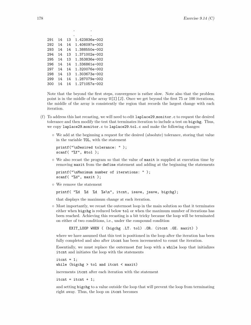
178 Exercise 9.14 (C)
. .
. .
291 14 13 1.423836e-002
292 14 14 1.406097e-002
293 14 14 1.388550e-002
294 14 13 1.371002e-002
295 14 13 1.353836e-002
296 14 14 1.336861e-002
297 14 14 1.320076e-002
298 14 13 1.303673e-002
299 14 14 1.287079e-002
300 14 14 1.271057e-002
Note that the beyond the first steps, convergence is rather slow. Note also that the problempoint is in the middle of the array U[I][J]. Once we get beyond the first 75 or 100 iterations,the middle of the array is consistently the region that records the largest change with eachiteration.
(f) To address this last recasting, we will need to edit laplace29 monitor.c to request the desiredtolerance and then modify the test that terminates iteration to include a test on bigchg. Thus,we copy laplace29 monitor.c to laplace29 tol.c and make the following changes:
We add at the beginning a request for the desired (absolute) tolerance, storing that valuein the variable TOL, with the statement
printf("\nDesired tolerance: " );
scanf( "%f", &tol );
We also recast the program so that the value of maxit is supplied at execution time byremoving maxit from the define statement and adding at the beginning the statements
printf("\nMaximum number of iterations: " );
scanf( "%d", maxit );
We remove the statement
printf( "%d %d %d %e\n", itcnt, isave, jsave, bigchg);
that displays the maximum change at each iteration.
Most importantly, we recast the outermost loop in the main solution so that it terminateseither when bigchg is reduced below tol or when the maximum number of iterations hasbeen reached. Achieving this recasting is a bit tricky because the loop will be terminatedon either of two conditions, i.e., under the compound condition
EXIT_LOOP WHEN ( (bigchg .LT. tol) .OR. (itcnt .GE. maxit) )
where we have assumed that this test is positioned in the loop after the iteration has beenfully completed and also after itcnt has been incremented to count the iteration.
Essentially, we must replace the outermost for loop with a while loop that initializesitcnt and initiates the loop with the statements
itcnt = 1;
while (bigchg > tol and itcnt < maxit)
increments itcnt after each iteration with the statement
itcnt = itcnt + 1;
and setting bigchg to a value outside the loop that will prevent the loop from terminatingright away. Thus, the loop on itcnt becomes
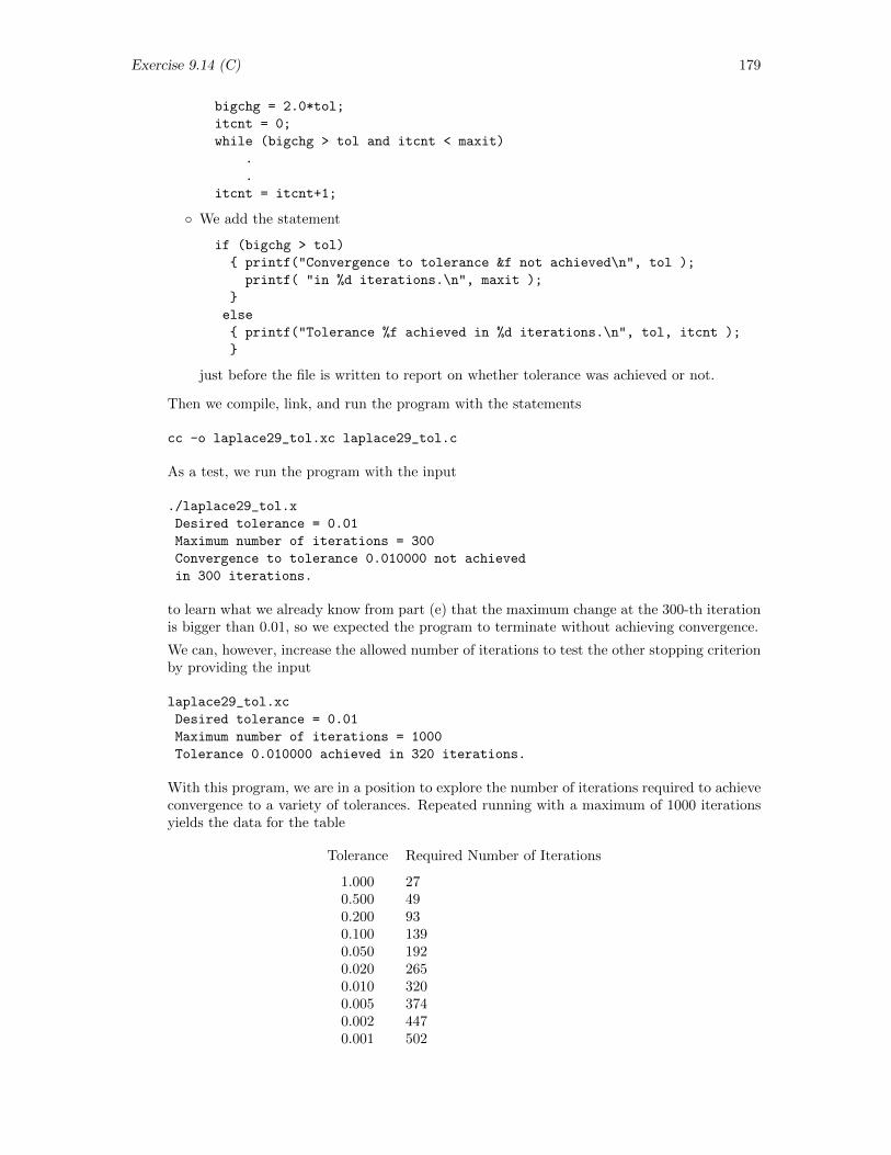
Exercise 9.14 (C) 179
bigchg = 2.0*tol;
itcnt = 0;
while (bigchg > tol and itcnt < maxit)
.
.
itcnt = itcnt+1;
We add the statement
if (bigchg > tol)
printf("Convergence to tolerance &f not achieved\n", tol );
printf( "in %d iterations.\n", maxit );
else
printf("Tolerance %f achieved in %d iterations.\n", tol, itcnt );
just before the file is written to report on whether tolerance was achieved or not.
Then we compile, link, and run the program with the statements
cc -o laplace29_tol.xc laplace29_tol.c
As a test, we run the program with the input
./laplace29_tol.x
Desired tolerance = 0.01
Maximum number of iterations = 300
Convergence to tolerance 0.010000 not achieved
in 300 iterations.
to learn what we already know from part (e) that the maximum change at the 300-th iterationis bigger than 0.01, so we expected the program to terminate without achieving convergence.
We can, however, increase the allowed number of iterations to test the other stopping criterionby providing the input
laplace29_tol.xc
Desired tolerance = 0.01
Maximum number of iterations = 1000
Tolerance 0.010000 achieved in 320 iterations.
With this program, we are in a position to explore the number of iterations required to achieveconvergence to a variety of tolerances. Repeated running with a maximum of 1000 iterationsyields the data for the table
Tolerance Required Number of Iterations
1.000 270.500 490.200 930.100 1390.050 1920.020 2650.010 3200.005 3740.002 4470.001 502
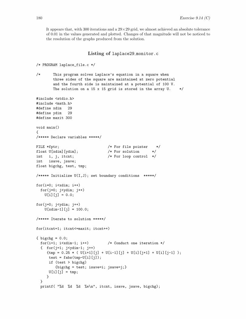
180 Exercise 9.14 (C)
It appears that, with 300 iterations and a 29×29 grid, we almost achieved an absolute toleranceof 0.01 in the values generated and plotted. Changes of that magnitude will not be noticed tothe resolution of the graphs produced from the solution.
Listing of laplace29 monitor.c
/* PROGRAM laplace_file.c */
/* This program solves Laplace’s equation in a square when
three sides of the square are maintained at zero potential
and the fourth side is maintained at a potential of 100 V.
The solution on a 15 x 15 grid is stored in the array U. */
#include <stdio.h>
#include <math.h>
#define xdim 29
#define ydim 29
#define maxit 300
void main()
/***** Declare variables *****/
FILE *fptr; /* For file pointer */
float U[xdim][ydim]; /* For solution */
int i, j, itcnt; /* For loop control */
int isave, jsave;
float bigchg, test, tmp;
/***** Initialize U(I,J); set boundary conditions *****/
for(i=0; i<xdim; i++)
for(j=0; j<ydim; j++)
U[i][j] = 0.0;
for(j=0; j<ydim; j++)
U[xdim-1][j] = 100.0;
/***** Iterate to solution *****/
for(itcnt=1; itcnt<=maxit; itcnt++)
bigchg = 0.0;
for(i=1; i<xdim-1; i++) /* Conduct one iteration */
for(j=1; j<ydim-1; j++)
tmp = 0.25 * ( U[i+1][j] + U[i-1][j] + U[i][j+1] + U[i][j-1] );
test = fabs(tmp-U[i][j]);
if (test > bigchg)
bigchg = test; isave=i; jsave=j;
U[i][j] = tmp;
printf( "%d %d %d %e\n", itcnt, isave, jsave, bigchg);
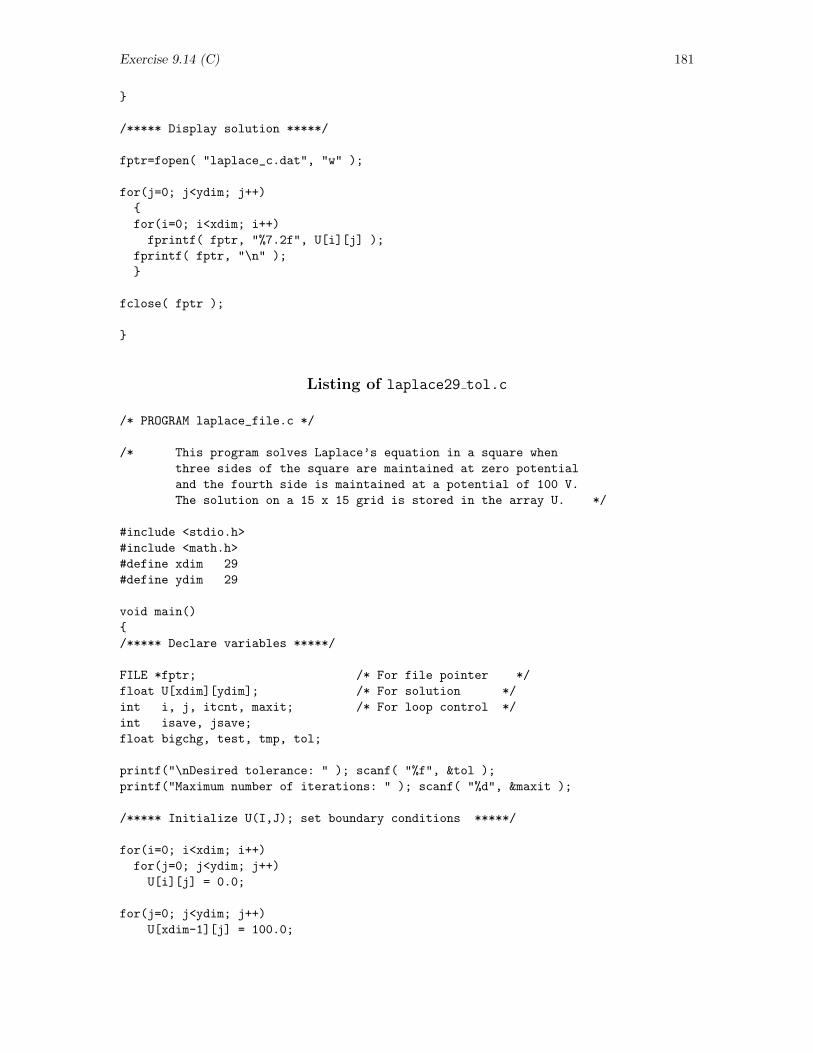
Exercise 9.14 (C) 181
/***** Display solution *****/
fptr=fopen( "laplace_c.dat", "w" );
for(j=0; j<ydim; j++)
for(i=0; i<xdim; i++)
fprintf( fptr, "%7.2f", U[i][j] );
fprintf( fptr, "\n" );
fclose( fptr );
Listing of laplace29 tol.c
/* PROGRAM laplace_file.c */
/* This program solves Laplace’s equation in a square when
three sides of the square are maintained at zero potential
and the fourth side is maintained at a potential of 100 V.
The solution on a 15 x 15 grid is stored in the array U. */
#include <stdio.h>
#include <math.h>
#define xdim 29
#define ydim 29
void main()
/***** Declare variables *****/
FILE *fptr; /* For file pointer */
float U[xdim][ydim]; /* For solution */
int i, j, itcnt, maxit; /* For loop control */
int isave, jsave;
float bigchg, test, tmp, tol;
printf("\nDesired tolerance: " ); scanf( "%f", &tol );
printf("Maximum number of iterations: " ); scanf( "%d", &maxit );
/***** Initialize U(I,J); set boundary conditions *****/
for(i=0; i<xdim; i++)
for(j=0; j<ydim; j++)
U[i][j] = 0.0;
for(j=0; j<ydim; j++)
U[xdim-1][j] = 100.0;
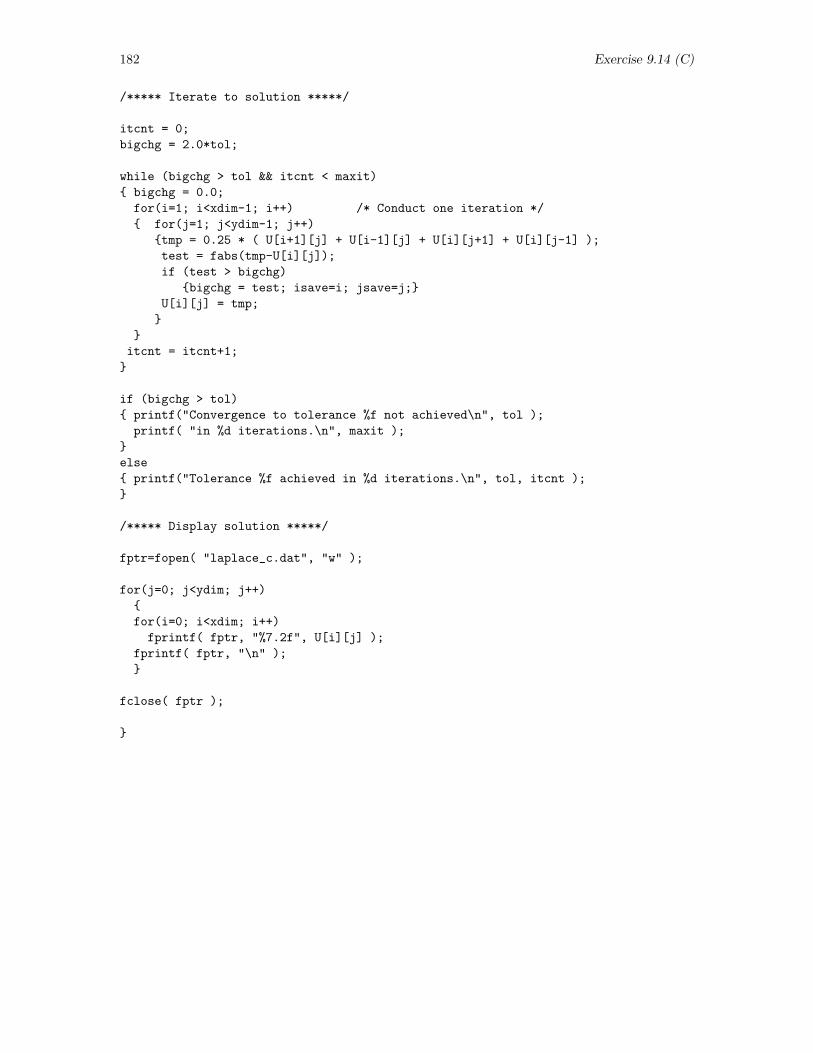
182 Exercise 9.14 (C)
/***** Iterate to solution *****/
itcnt = 0;
bigchg = 2.0*tol;
while (bigchg > tol && itcnt < maxit)
bigchg = 0.0;
for(i=1; i<xdim-1; i++) /* Conduct one iteration */
for(j=1; j<ydim-1; j++)
tmp = 0.25 * ( U[i+1][j] + U[i-1][j] + U[i][j+1] + U[i][j-1] );
test = fabs(tmp-U[i][j]);
if (test > bigchg)
bigchg = test; isave=i; jsave=j;
U[i][j] = tmp;
itcnt = itcnt+1;
if (bigchg > tol)
printf("Convergence to tolerance %f not achieved\n", tol );
printf( "in %d iterations.\n", maxit );
else
printf("Tolerance %f achieved in %d iterations.\n", tol, itcnt );
/***** Display solution *****/
fptr=fopen( "laplace_c.dat", "w" );
for(j=0; j<ydim; j++)
for(i=0; i<xdim; i++)
fprintf( fptr, "%7.2f", U[i][j] );
fprintf( fptr, "\n" );
fclose( fptr );
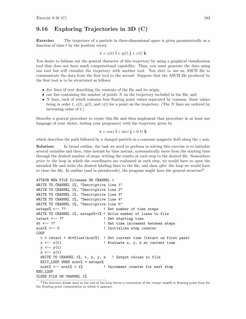
Exercise 9.16 (C) 183
9.16 Exploring Trajectories in 3D (C)
Exercise: The trajectory of a particle in three-dimensional space is given parametrically as afunction of time t by the position vector
r = x(t) i + y(t) j + z(t) k
You desire to fathom out the general character of this trajectory by using a graphical visualizationtool that does not have much computational capability. Thus, you must generate the data usingone tool but will visualize the trajectory with another tool. You elect to use an ASCII file tocommunicate the data from the first tool to the second. Suppose that the ASCII file produced bythe first tool is to be structured as follows:
• five lines of text describing the contents of the file and its origin,• one line containing the number of points N on the trajectory included in the file, and• N lines, each of which contains four floating point values separated by commas, those values
being in order t, x(t), y(t), and z(t) for a point on the trajectory. (The N lines are ordered byincreasing value of t.)
Describe a general procedure to create this file and then implement that procedure in at least onelanguage of your choice, testing your program(s) with the trajectory given by
r = cos t i + sin t j + 0.1t k
which describes the path followed by a charged particle in a constant magnetic field along the z axis.
Solution: In broad outline, the task we need to perform in solving this exercise is to initializeseveral variables and then, time instant by time instant, systematically move from the starting timethrough the desired number of steps, writing the results at each step to the desired file. Somewhereprior to the loop in which the coordinates are evaluated at each step, we would have to open theintended file and write the desired labeling lines to the file, and then after the loop we would haveto close the file. In outline (and in pseudocode), the program might have the general structure6
ATTACH NEW FILE filename ON CHANNEL 1
WRITE TO CHANNEL 1%, "Descriptive line 1"
WRITE TO CHANNEL 1%, "Descriptive line 2"
WRITE TO CHANNEL 1%, "Descriptive line 3"
WRITE TO CHANNEL 1%, "Descriptive line 4"
WRITE TO CHANNEL 1%, "Descriptive line 5"
nsteps% <-- ?? ! Set number of time steps
WRITE TO CHANNEL 1%, nsteps%+1% ! Write number of lines to file
tstart <-- ?? ! Set starting time
dt <-- ?? ! Set time increment between steps
ncnt% <-- 0 ! Initialize step counter
LOOP
t = tstart + dt*float(ncnt%) ! Set current time (tstart on first pass)
x <-- x(t) ! Evaluate x, y, z at current time
y <-- y(t)
z <-- z(t)
WRITE TO CHANNEL 1%, t, x, y, z ! Output values to file
EXIT_LOOP WHEN ncnt% = nsteps%
ncnt% <-- ncnt% + 1% ! Increment counter for next step
END_LOOP
CLOSE FILE ON CHANNEL 1%
6The function float used at the end of the loop forces a conversion of the integer ncnt% to floating point form forthe floating-point computation in which it appears.
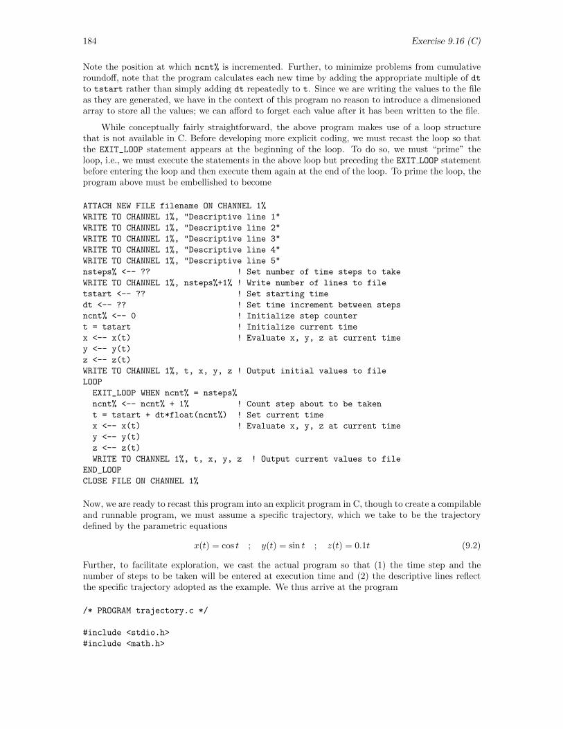
184 Exercise 9.16 (C)
Note the position at which ncnt% is incremented. Further, to minimize problems from cumulativeroundoff, note that the program calculates each new time by adding the appropriate multiple of dtto tstart rather than simply adding dt repeatedly to t. Since we are writing the values to the fileas they are generated, we have in the context of this program no reason to introduce a dimensionedarray to store all the values; we can afford to forget each value after it has been written to the file.
While conceptually fairly straightforward, the above program makes use of a loop structurethat is not available in C. Before developing more explicit coding, we must recast the loop so thatthe EXIT_LOOP statement appears at the beginning of the loop. To do so, we must “prime” theloop, i.e., we must execute the statements in the above loop but preceding the EXIT LOOP statementbefore entering the loop and then execute them again at the end of the loop. To prime the loop, theprogram above must be embellished to become
ATTACH NEW FILE filename ON CHANNEL 1%
WRITE TO CHANNEL 1%, "Descriptive line 1"
WRITE TO CHANNEL 1%, "Descriptive line 2"
WRITE TO CHANNEL 1%, "Descriptive line 3"
WRITE TO CHANNEL 1%, "Descriptive line 4"
WRITE TO CHANNEL 1%, "Descriptive line 5"
nsteps% <-- ?? ! Set number of time steps to take
WRITE TO CHANNEL 1%, nsteps%+1% ! Write number of lines to file
tstart <-- ?? ! Set starting time
dt <-- ?? ! Set time increment between steps
ncnt% <-- 0 ! Initialize step counter
t = tstart ! Initialize current time
x <-- x(t) ! Evaluate x, y, z at current time
y <-- y(t)
z <-- z(t)
WRITE TO CHANNEL 1%, t, x, y, z ! Output initial values to file
LOOP
EXIT_LOOP WHEN ncnt% = nsteps%
ncnt% <-- ncnt% + 1% ! Count step about to be taken
t = tstart + dt*float(ncnt%) ! Set current time
x <-- x(t) ! Evaluate x, y, z at current time
y <-- y(t)
z <-- z(t)
WRITE TO CHANNEL 1%, t, x, y, z ! Output current values to file
END_LOOP
CLOSE FILE ON CHANNEL 1%
Now, we are ready to recast this program into an explicit program in C, though to create a compilableand runnable program, we must assume a specific trajectory, which we take to be the trajectorydefined by the parametric equations
x(t) = cos t ; y(t) = sin t ; z(t) = 0.1t (9.2)
Further, to facilitate exploration, we cast the actual program so that (1) the time step and thenumber of steps to be taken will be entered at execution time and (2) the descriptive lines reflectthe specific trajectory adopted as the example. We thus arrive at the program
/* PROGRAM trajectory.c */
#include <stdio.h>
#include <math.h>
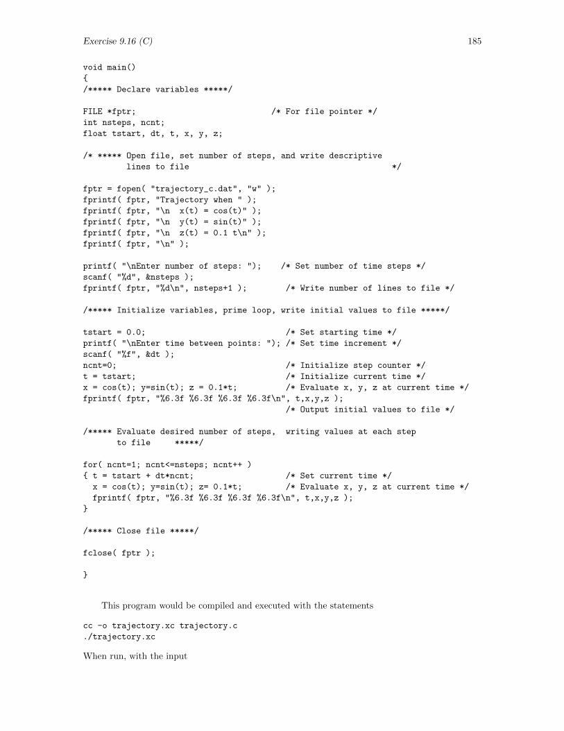
Exercise 9.16 (C) 185
void main()
/***** Declare variables *****/
FILE *fptr; /* For file pointer */
int nsteps, ncnt;
float tstart, dt, t, x, y, z;
/* ***** Open file, set number of steps, and write descriptive
lines to file */
fptr = fopen( "trajectory_c.dat", "w" );
fprintf( fptr, "Trajectory when " );
fprintf( fptr, "\n x(t) = cos(t)" );
fprintf( fptr, "\n y(t) = sin(t)" );
fprintf( fptr, "\n z(t) = 0.1 t\n" );
fprintf( fptr, "\n" );
printf( "\nEnter number of steps: "); /* Set number of time steps */
scanf( "%d", &nsteps );
fprintf( fptr, "%d\n", nsteps+1 ); /* Write number of lines to file */
/***** Initialize variables, prime loop, write initial values to file *****/
tstart = 0.0; /* Set starting time */
printf( "\nEnter time between points: "); /* Set time increment */
scanf( "%f", &dt );
ncnt=0; /* Initialize step counter */
t = tstart; /* Initialize current time */
x = cos(t); y=sin(t); z = 0.1*t; /* Evaluate x, y, z at current time */
fprintf( fptr, "%6.3f %6.3f %6.3f %6.3f\n", t,x,y,z );
/* Output initial values to file */
/***** Evaluate desired number of steps, writing values at each step
to file *****/
for( ncnt=1; ncnt<=nsteps; ncnt++ )
t = tstart + dt*ncnt; /* Set current time */
x = cos(t); y=sin(t); z= 0.1*t; /* Evaluate x, y, z at current time */
fprintf( fptr, "%6.3f %6.3f %6.3f %6.3f\n", t,x,y,z );
/***** Close file *****/
fclose( fptr );
This program would be compiled and executed with the statements
cc -o trajectory.xc trajectory.c
./trajectory.xc
When run, with the input
186 Exercise 9.16 (C)
Enter number of steps: 10
Enter time between points: 0.1
the resulting file trajectory c.dat contains the lines
Trajectory when
x(t) = cos(t)
y(t) = sin(t)
z(t) = 0.1 t
11
0.000 1.000 0.000 0.000
0.100 0.995 0.100 0.010
0.200 0.980 0.199 0.020
0.300 0.955 0.296 0.030
0.400 0.921 0.389 0.040
0.500 0.878 0.479 0.050
0.600 0.825 0.565 0.060
0.700 0.765 0.644 0.070
0.800 0.697 0.717 0.080
0.900 0.622 0.783 0.090
1.000 0.540 0.841 0.100
To produce the desired graphical display of this trajectory, we need to input this file into asuitable graphics program. In IDL, we would execute the statements
ln = "" ; Set string variable for reading lines
openr, 1, ’trajectory_c.dat’ ; Open file
for i=1,5 do readf, 1, ln ; Read past and ignore first 5 lines
readf, 1, nlines ; Read number of lines
traj = fltarr(4,nlines) ; Dimension array for data
readf, 1, traj ; Read data
close, 1 ; Close the file
t = traj[0,*] & x = traj[1,*] & y = traj[2,*] & z = traj[3,*]
to open the file, read past the descriptive lines, read the data contained in the file, close the file, and(for convenience in reference) extract each column into a more mnemonically named variable. Then,to display the trajectory in a graph, we execute the statements (see Section 2.16.2 of CPSUP)
scale3, xrange=[-1.0,1.0], yrange=[-1.0,1.0], zrange=[0.0,0.1]
plots, x, y, z, /t3d
The scaling was determined by noting that −1.0 ≤ x, y ≤ 1.0 (since those are the limits on the sineand cosine functions) and 0 ≤ z ≤ 0.1.
The sample above, of course, did not trace the trajectory very far away from its origin. To finda more suitable total time interval, we note that x and y each take time 2π to complete one cycle. Ifwe want to plot the trajectory through, say, 4 full cycles, we should allow t to run from 0 to about8π ≈ 25.0, whence z will run from 0 to 2.5. If we rerun the program with the input
Enter number of steps: 250
Enter time between points: 0.1
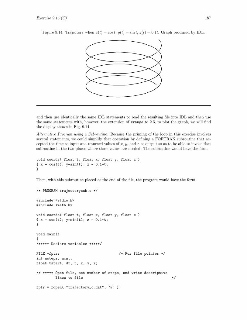
Exercise 9.16 (C) 187
Figure 9.14: Trajectory when x(t) = cos t, y(t) = sin t, z(t) = 0.1t. Graph produced by IDL.
and then use identically the same IDL statements to read the resulting file into IDL and then usethe same statements with, however, the extension of zrange to 2.5, to plot the graph, we will findthe display shown in Fig. 9.14.
Alternative Program using a Subroutine: Because the priming of the loop in this exercise involvesseveral statements, we could simplify that operation by defining a FORTRAN subroutine that ac-cepted the time as input and returned values of x, y, and z as output so as to be able to invoke thatsubroutine in the two places where those values are needed. The subroutine would have the form
void coords( float t, float x, float y, float z )
x = cos(t); y=sin(t); z = 0.1*t;
Then, with this subroutine placed at the end of the file, the program would have the form
/* PROGRAM trajectorysub.c */
#include <stdio.h>
#include <math.h>
void coords( float t, float x, float y, float z )
x = cos(t); y=sin(t); z = 0.1*t;
void main()
/***** Declare variables *****/
FILE *fptr; /* For file pointer */
int nsteps, ncnt;
float tstart, dt, t, x, y, z;
/* ***** Open file, set number of steps, and write descriptive
lines to file */
fptr = fopen( "trajectory_c.dat", "w" );
188 Exercise 9.16 (C)
fprintf( fptr, "Trajectory when " );
fprintf( fptr, "\n x(t) = cos(t)" );
fprintf( fptr, "\n y(t) = sin(t)" );
fprintf( fptr, "\n z(t) = 0.1 t\n" );
fprintf( fptr, "\n" );
printf( "\nEnter number of steps: "); /* Set number of time steps */
scanf( "%d", &nsteps );
fprintf( fptr, "%d\n", nsteps+1 ); /* Write number of lines to file */
/***** Initialize variables, prime loop, write initial values to file *****/
tstart = 0.0; /* Set starting time */
printf( "\nEnter time between points: "); /* Set time increment */
scanf( "%f", &dt );
ncnt=0; /* Initialize step counter */
t = tstart; /* Initialize current time */
coords( t, x, y, z); /* Evaluate x, y, z at current time */
fprintf( fptr, "%6.3f %6.3f %6.3f %6.3f\n", t,x,y,z );
/* Output initial values to file */
/***** Evaluate desired number of steps, writing values at each step
to file *****/
for( ncnt=1; ncnt<=nsteps; ncnt++ )
t = tstart + dt*ncnt; /* Set current time */
coords( t, x, y, z); /* Evaluate x, y, z at current time */
fprintf( fptr, "%6.3f %6.3f %6.3f %6.3f\n", t,x,y,z );
/***** Close file *****/
fclose( fptr );
This program would be compiled and executed with the statements
cc -o trajectoryseb.xc trajectoryseb.c
./trajectorysub.xc
When run, with the input
Enter number of steps: 10
Enter time between points: 0.1
the resulting file trajectory c.dat would be the same as the corresponding file displayed earlier.
Exercise 9.22 (C) 189
9.22 Great Circle Distances (C)
Exercise: Write and test a program to ask for the latitude and longitude of both a point ofdeparture D and a point of arrival A on the surface of the earth and then calculate and print outthe “crow-flies” distance along a great circle route from D to A. Make sure your program prints theshorter of the two distances, regardless of the location of the points, and make sure your programdoesn’t run into difficulties if the two points happen to be at opposite ends of a diameter. Take theearth to be a perfect sphere with a circumference of 24900 miles (radius 3963 miles). For purposesof testing, note that Albany, NY, is at [4340′ N, 7345′ W]; Grand Junction, CO, is at [395′ N,10833′ W]; Los Angeles, CA, is at [343′ N, 11815′ W]; Appleton, WI, is at [4416′ N, 8825′ W];Calcutta India, is at [2232′ N, 8820′ E]; Sydney, Australia, is at [3352′ S, 15112′ E]; Paris,France, is at [4849′ N, 229′ E]; and Stockholm, Sweden, is at [5921′ N, 184′ E].
Solution: Introduce a coordinate system in which the axis of the earth defines the z axis, a linefrom the center of the earth to the equator at a point at longitude of 0 defines the x axis, and a linefrom the center of the earth to the equation at a point at longitude 90 E. In that system, let thepolar and azimuthal angles (not the latitude and longitude) of one point be θ1, φ1 and the polar andazimuthal angles of the other point be θ2, φ2, where 0 ≤ θ1, θ2 ≤ 90 and −180 ≤ φ1, φ2 ≤ 180.Further, let the radius of the earth, considered to be a sphere, be R. Then vector r1 and r2 fromthe center of the earth to each of these points are given by
r1 = R(sin θ1 cosφ1 i + sin θ1 sinφ1 j + cos θ1 k
)and
r2 = R(sin θ2 cosφ2 i + sin θ2 sinφ2 j + cos θ2 k
)Remembering that the dot product of two vectors A and B is defined by
A •B = |A| |B| cos θAB =⇒ cos θAB =A •B|A| |B|
we conclude that the angle subtended at the center of the earth by the two vectors identifying thepoints of interest on the earth’s surface is given by
θ12 = cos−1
(r1 • r2
r1 r2
)=
r1
R• r2
R
and then that the required distance is given by
d = Rθ12
A listing of a program to accomplish the desired task is presented at the end of this solution. Thetask is complicated a bit because the input information is to be given in terms of the normal latitude-longitude designation of the points of interest, e.g., Albany, NY, at 42 40′ N latitude, 73 45′ Wlongitude. Thus, the first task of the program before calculating the distance between two pointsso specified is to obtain the input coordinates in the conventional terminology and then convertthat specification for each into the polar and azimuthal angles involved in the above expressionsfor the radius vectors of the two points. We will use implicit variable typing, except that we needto declare explicitly four character variables to contain single characters N or S for latitude, E orW longitude. Using S as the initial character of a variable pertaining to the starting point and E
as the initial character for the ending point, LAT and LON to convey latitude and longitude, andDEG and MIN in a variable name to convey degrees and minutes, we begin—Section 1—by declaringfour character variables that will ultimately contain the latitude and longitude of each point ofinterest and dimensioning two vectors that will ultimately contain the three components of the twovectors r1/R and r2/R. Then—Section 2—we set important constants. Next—Section 3—we printinstructions to clarify the way in which input data will be provided. In Section 4, we actually obtainthe input data, storing the three values for each latitude and longitude in three separate variables.
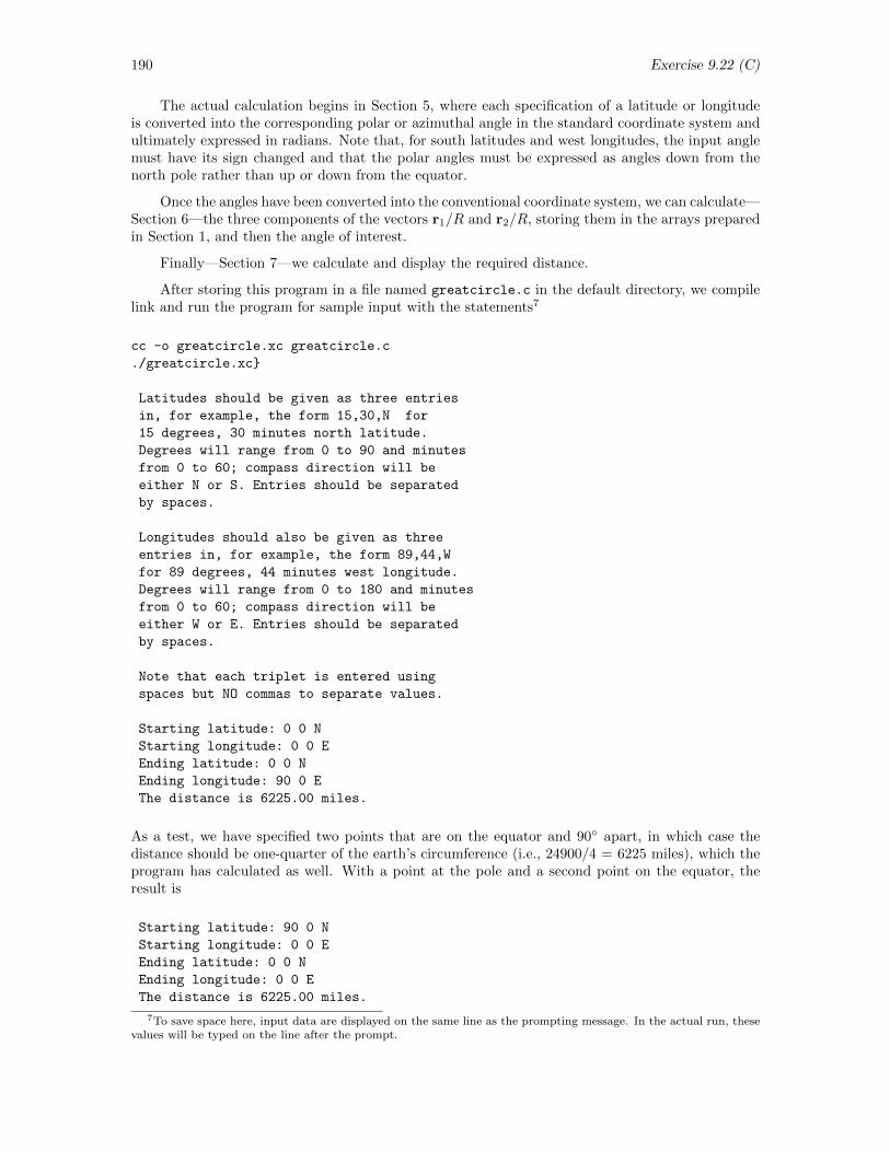
190 Exercise 9.22 (C)
The actual calculation begins in Section 5, where each specification of a latitude or longitudeis converted into the corresponding polar or azimuthal angle in the standard coordinate system andultimately expressed in radians. Note that, for south latitudes and west longitudes, the input anglemust have its sign changed and that the polar angles must be expressed as angles down from thenorth pole rather than up or down from the equator.
Once the angles have been converted into the conventional coordinate system, we can calculate—Section 6—the three components of the vectors r1/R and r2/R, storing them in the arrays preparedin Section 1, and then the angle of interest.
Finally—Section 7—we calculate and display the required distance.
After storing this program in a file named greatcircle.c in the default directory, we compilelink and run the program for sample input with the statements7
cc -o greatcircle.xc greatcircle.c
./greatcircle.xc
Latitudes should be given as three entries
in, for example, the form 15,30,N for
15 degrees, 30 minutes north latitude.
Degrees will range from 0 to 90 and minutes
from 0 to 60; compass direction will be
either N or S. Entries should be separated
by spaces.
Longitudes should also be given as three
entries in, for example, the form 89,44,W
for 89 degrees, 44 minutes west longitude.
Degrees will range from 0 to 180 and minutes
from 0 to 60; compass direction will be
either W or E. Entries should be separated
by spaces.
Note that each triplet is entered using
spaces but NO commas to separate values.
Starting latitude: 0 0 N
Starting longitude: 0 0 E
Ending latitude: 0 0 N
Ending longitude: 90 0 E
The distance is 6225.00 miles.
As a test, we have specified two points that are on the equator and 90 apart, in which case thedistance should be one-quarter of the earth’s circumference (i.e., 24900/4 = 6225 miles), which theprogram has calculated as well. With a point at the pole and a second point on the equator, theresult is
Starting latitude: 90 0 N
Starting longitude: 0 0 E
Ending latitude: 0 0 N
Ending longitude: 0 0 E
The distance is 6225.00 miles.
7To save space here, input data are displayed on the same line as the prompting message. In the actual run, thesevalues will be typed on the line after the prompt.
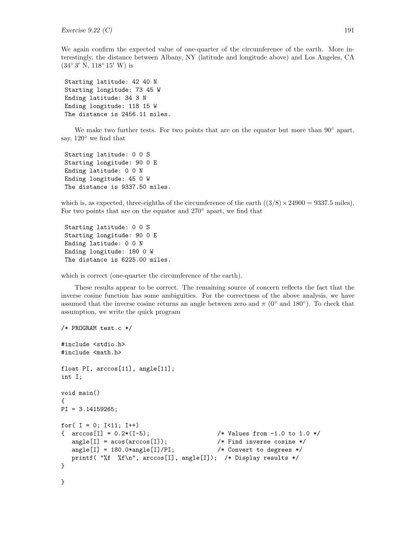
Exercise 9.22 (C) 191
We again confirm the expected value of one-quarter of the circumference of the earth. More in-terestingly, the distance between Albany, NY (latitude and longitude above) and Los Angeles, CA(34 3′ N, 118 15′ W) is
Starting latitude: 42 40 N
Starting longitude: 73 45 W
Ending latitude: 34 3 N
Ending longitude: 118 15 W
The distance is 2456.11 miles.
We make two further tests. For two points that are on the equator but more than 90 apart,say, 120 we find that
Starting latitude: 0 0 S
Starting longitude: 90 0 E
Ending latitude: 0 0 N
Ending longitude: 45 0 W
The distance is 9337.50 miles.
which is, as expected, three-eighths of the circumference of the earth ((3/8)×24900 = 9337.5 miles).For two points that are on the equator and 270 apart, we find that
Starting latitude: 0 0 S
Starting longitude: 90 0 E
Ending latitude: 0 0 N
Ending longitude: 180 0 W
The distance is 6225.00 miles.
which is correct (one-quarter the circumference of the earth).
These results appear to be correct. The remaining source of concern reflects the fact that theinverse cosine function has some ambiguities. For the correctness of the above analysis, we haveassumed that the inverse cosine returns an angle between zero and π (0 and 180). To check thatassumption, we write the quick program
/* PROGRAM test.c */
#include <stdio.h>
#include <math.h>
float PI, arccos[11], angle[11];
int I;
void main()
PI = 3.14159265;
for( I = 0; I<11; I++)
arccos[I] = 0.2*(I-5); /* Values from -1.0 to 1.0 */
angle[I] = acos(arccos[I]); /* Find inverse cosine */
angle[I] = 180.0*angle[I]/PI; /* Convert to degrees */
printf( "%f %f\n", arccos[I], angle[I]); /* Display results */
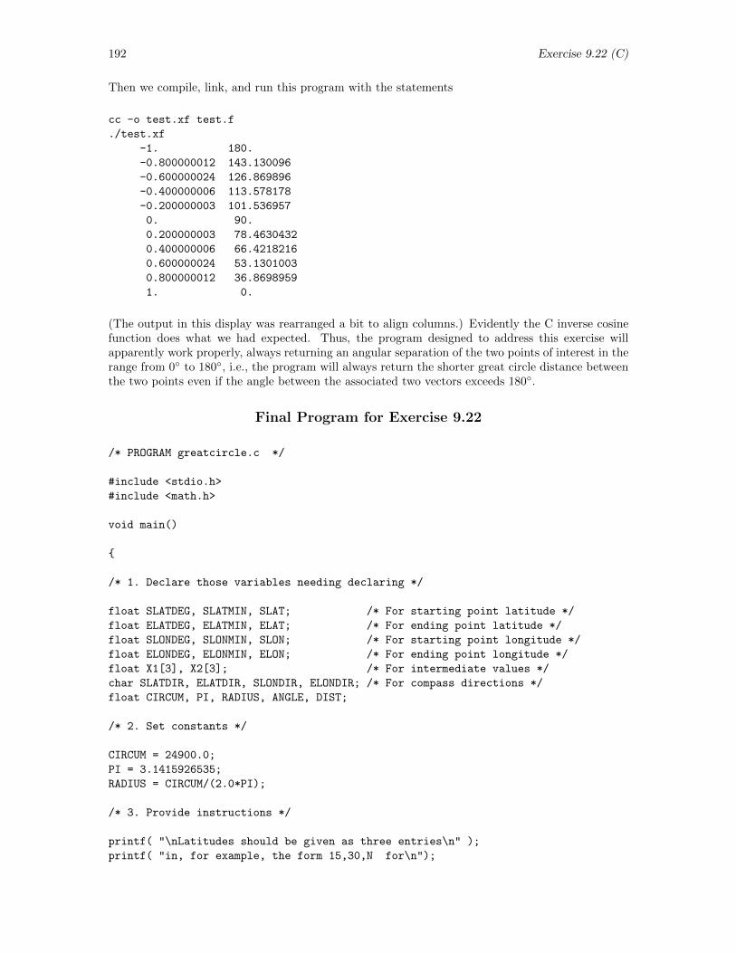
192 Exercise 9.22 (C)
Then we compile, link, and run this program with the statements
cc -o test.xf test.f
./test.xf
-1. 180.
-0.800000012 143.130096
-0.600000024 126.869896
-0.400000006 113.578178
-0.200000003 101.536957
0. 90.
0.200000003 78.4630432
0.400000006 66.4218216
0.600000024 53.1301003
0.800000012 36.8698959
1. 0.
(The output in this display was rearranged a bit to align columns.) Evidently the C inverse cosinefunction does what we had expected. Thus, the program designed to address this exercise willapparently work properly, always returning an angular separation of the two points of interest in therange from 0 to 180, i.e., the program will always return the shorter great circle distance betweenthe two points even if the angle between the associated two vectors exceeds 180.
Final Program for Exercise 9.22
/* PROGRAM greatcircle.c */
#include <stdio.h>
#include <math.h>
void main()
/* 1. Declare those variables needing declaring */
float SLATDEG, SLATMIN, SLAT; /* For starting point latitude */
float ELATDEG, ELATMIN, ELAT; /* For ending point latitude */
float SLONDEG, SLONMIN, SLON; /* For starting point longitude */
float ELONDEG, ELONMIN, ELON; /* For ending point longitude */
float X1[3], X2[3]; /* For intermediate values */
char SLATDIR, ELATDIR, SLONDIR, ELONDIR; /* For compass directions */
float CIRCUM, PI, RADIUS, ANGLE, DIST;
/* 2. Set constants */
CIRCUM = 24900.0;
PI = 3.1415926535;
RADIUS = CIRCUM/(2.0*PI);
/* 3. Provide instructions */
printf( "\nLatitudes should be given as three entries\n" );
printf( "in, for example, the form 15,30,N for\n");
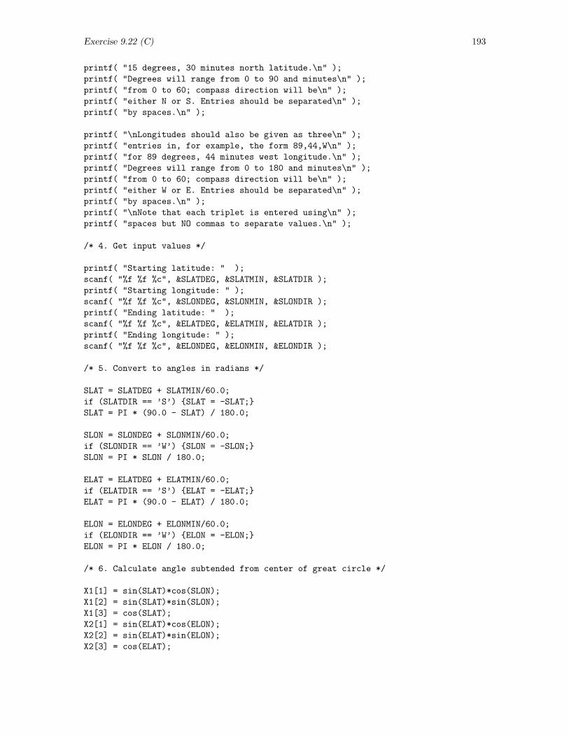
Exercise 9.22 (C) 193
printf( "15 degrees, 30 minutes north latitude.\n" );
printf( "Degrees will range from 0 to 90 and minutes\n" );
printf( "from 0 to 60; compass direction will be\n" );
printf( "either N or S. Entries should be separated\n" );
printf( "by spaces.\n" );
printf( "\nLongitudes should also be given as three\n" );
printf( "entries in, for example, the form 89,44,W\n" );
printf( "for 89 degrees, 44 minutes west longitude.\n" );
printf( "Degrees will range from 0 to 180 and minutes\n" );
printf( "from 0 to 60; compass direction will be\n" );
printf( "either W or E. Entries should be separated\n" );
printf( "by spaces.\n" );
printf( "\nNote that each triplet is entered using\n" );
printf( "spaces but NO commas to separate values.\n" );
/* 4. Get input values */
printf( "Starting latitude: " );
scanf( "%f %f %c", &SLATDEG, &SLATMIN, &SLATDIR );
printf( "Starting longitude: " );
scanf( "%f %f %c", &SLONDEG, &SLONMIN, &SLONDIR );
printf( "Ending latitude: " );
scanf( "%f %f %c", &ELATDEG, &ELATMIN, &ELATDIR );
printf( "Ending longitude: " );
scanf( "%f %f %c", &ELONDEG, &ELONMIN, &ELONDIR );
/* 5. Convert to angles in radians */
SLAT = SLATDEG + SLATMIN/60.0;
if (SLATDIR == ’S’) SLAT = -SLAT;
SLAT = PI * (90.0 - SLAT) / 180.0;
SLON = SLONDEG + SLONMIN/60.0;
if (SLONDIR == ’W’) SLON = -SLON;
SLON = PI * SLON / 180.0;
ELAT = ELATDEG + ELATMIN/60.0;
if (ELATDIR == ’S’) ELAT = -ELAT;
ELAT = PI * (90.0 - ELAT) / 180.0;
ELON = ELONDEG + ELONMIN/60.0;
if (ELONDIR == ’W’) ELON = -ELON;
ELON = PI * ELON / 180.0;
/* 6. Calculate angle subtended from center of great circle */
X1[1] = sin(SLAT)*cos(SLON);
X1[2] = sin(SLAT)*sin(SLON);
X1[3] = cos(SLAT);
X2[1] = sin(ELAT)*cos(ELON);
X2[2] = sin(ELAT)*sin(ELON);
X2[3] = cos(ELAT);

194 Exercise 9.22 (C)
ANGLE = X1[1]*X2[1] + X1[2]*X2[2] + X1[3]*X2[3];
ANGLE = acos( ANGLE );
/* 7. Calculate and display distance */
DIST = ANGLE * RADIUS;
printf( "The distance is %7.2f miles.", DIST);
Chapter 11
Solving ODEs
11.1 Driven oscillator (Mathematica)
Exercise: Find the motion of a driven, damped oscillator satisfying the differential equation
md2x
dt2+ b
dx
dt+ kx = mf cosωt
subject to the general initial conditions
x(0) = x0 ;dx
dt(0) = v0
and then determine the particular initial values that might be imposed so that the transient partof the solution is wiped out from the beginning, i.e., so that the motion is identically the steady-state motion from the moment the oscillator is set into motion. Assume that the oscillator isunderdamped. (Note that, so that m will ultimately appear only in conjunction with b and k, wehave chosen to define f as a force per unit mass rather than simply a force.)
Solution: To solve the given differential equation with Mathematica, we begin by defining thedifferential equation with the statement
In[1]:= odeqn = m*D[x[t], t, 2] + b*D[x[t], t, 1] + k*x[t] ==
m*f*Cos[\[Omega]*t]
Out[1]= k x(t) + b x′(t) +mx′′(t) = f m cos(t ω)
the initial conditions with the statement
In[2]:= ics = x[0] == x0, x’[0] == v0
Out[2]= x(0) = x0, x′(0) = v0
As illustrated in Section 8.9 of the Mathematica chapter in CPSUP, we must take many steps afterinvoking DSolve with the statement
In[3]:= soln1 = DSolve[ odeqn, ics, x[t], t ];
to specify that we want the case of underdamped motion. To tell Mathematica that b2 < 4km, andthen to find a solution in the form of underdamped motion, we follow the lead of the above-referencedsection and execute the statements
195
196 Exercise 11.1 (Mathematica)
In[4]:= soln2 = soln1[[1]][[1]][[2]];
In[5]:= soln3 = Simplify[ soln2, m > 0 ];
In[6]:= soln4 = soln3 /. Sqrt[b^2 - 4*k*m] -> I*a;
In[7]:= Part[ soln4, 3 ]
Out[7]=1√
b2 − 4 km
In[8]:= soln4 = soln4 /. Part[soln4, 3] -> 1/(I*a);
In[9]:= soln5 = Expand[soln4];
In[10]:= soln6 = Map[ ComplexExpand, soln5, 6 ];
In[11]:= soln7 = Simplify[ soln6, b*t/m > 0 ];
In[12]:= soln8 = Collect[ soln7, Cos[\[Omega]*t], Sin[\[Omega]*t ],
Cos[a*t/(2*m)], Sin[a*t/(2*m)]];
In[13]:= soln9 = soln8 /. a -> Sqrt[b^2 - 4*k*m];
In[14]:= soln10 = x[t] -> soln9
Out[14]= Ae−bt/2m cos
√4km− b2 t
2m+B cos(ωt) + Fe−bt/2m sin
√4km− b2 t
2m+G sin(ωt)
We have suppressed explicit inclusion of the values Mathematica gives for the coefficients A, B, F ,and G. (C, D, and E are protected variables.) Hiding those complexities, we then see more clearlythat the solution consists of four terms. In the result we have obtained, the terms multiplied by adecaying exponential will disappear as t becomes large. Thus, the first and third terms constitutethe transient part of the solution and the second and fourth terms constitute the steady state part.
To be sure, Mathematica indeed returns explicit values for the constants A, B, F , and G. For thesake of completeness, we use Mathematica as follows to extract and simplify these four coefficients.For the coefficient A, we would execute the statement1
In[15]:= A = Part[ soln10[[1]][[1]][[2]], 1 ]/(Cos[Sqrt[b^2 - 4*k*m]*t/(2*m)]*
Exp[-b*t/(2*m)])
Out[15]=fm(−k +mω2) + x0
(k2 + b2ω2 − 2kmω2 +m2ω4
)k2 + b2ω2 − 2kmω2 +m2ω4
where we find the first term of the solution with the Part function and then divide out the parts ofthe first term that are not part of the coefficient.
Essentially similar statements will extract the remaining three coefficients from the originalsolution. However, more statements are needed to simplify the numerator in F . We find that
In[16]:= B = Part[ soln10[[1]][[1]][[2]], 2 ]/Cos[t*\[Omega]]
Out[16]= −(
fm(−k +mω2)
k2 + b2ω2 − 2kmω2 +m2ω4
)In[17]:= F = Part[ soln10[[1]][[1]][[2]], 3 ]/(Sin[Sqrt[b^2 - 4*k*m]*t/(2*m)]*
Exp[-b*t/(2*m)]);
In[18]:= num = Collect[ Numerator[F], x0, v0 ];
In[19]:= F = num/Denominator[F]
1Warning: Mathematica does not in all circumstances present the four terms in this solution in the same order.Thus, the numbers needed to extract the coefficients of the terms with sine or cosine factors may be different in yoursession than they are here. Beware!
Exercise 11.1 (Mathematica) 197
Out[19]=
−(bfkm)− bfm2ω2 + x0(bk2 + b3ω2 − 2bkmω2 + bm2ω4)
+v0(2k2m+ 2b2mω2 − 4km2ω2 + 2m3ω4)√b2 − 4km(k2 + b2ω2 − 2kmω2 +m2ω4)
In[20]:= G = Part[ soln10[[1]][[1]][[2]],4]/Sin[t*\[Omega] ]
Out[20]=bfmω
k2 + b2ω2 − 2kmω2 +m2ω4
To achieve the objective of the problem, we want to find initial conditions that will result in thetransient terms having zero coefficients so that, in fact, the transient term is gone from the beginning.Evidently, because the sine and cosine functions are linearly independent of one another, we cannot“wipe out” the transient term as required unless the coefficients of the sine and cosine terms areseparately zero. Thus, to eliminate the transient term from the beginning, we must require that
A = 0 and B = 0
Our remaining task in Mathematica then is simply to solve these two equations for the initial values,x0 and v0. Each of these results, however, is a fraction whose denominator is not zero. Thus, therequired coefficients will be zero if the numerators are zero, and we finally find that the equationswe wish to solve for x0 and v0 are
In[21]:= eq1 = Numerator[F] == 0
Out[21]= −(bfkm)− bfm2ω2 + x0
(bk2 + b3ω2 − 2bkmω2 + bm2ω4
)+
v0(2k2m+ 2b2mω2 − 4km2ω2 + 2m3ω4) = 0
In[22]:= eq2 = Numerator[A] == 0
Out[22]= fm(−k +mω2) + x0(k2 + b2ω2 − 2kmω2 +m2ω4) = 0
Finally, we determine the desired initial conditions with the statements
In[23]:= notran = Solve[ eq1, eq2, x0, v0 ]
Out[23]=
v0 →
bfmω2
k2 + b2ω2 − 2kmω2 +m2ω4, x0 → −
(fm(−k +mω2)
k2 + b2ω2 − 2kmω2 +m2ω4
)Then, if we substitute these results into the original solution with the statements
In[24]:= soln10 /. x0 -> notran[[1]][[2]][[2]], v0 -> notran[[1]][[1]][[2]];
In[25]:= Simplify[%]
Out[25]=
x(t)→
fm((k −mω2
)cos(tω) + bω sin(tω)
)k2 + b2ω2 − 2kmω2 +m2ω4
we confirm that, with the identified initial conditions, the steady state solution describes the motionright from time t = 0.
Note that the denominator in the solutions for x0 and v0 can be rewritten in the slightly moretransparent form
k2 − 2kω2m+ ω2b2 + ω4m2 = (k − ω2m)2 + ω2b2
and that, if we limit the frequency of the driving force to the natural frequency of the undampedoscillator, i.e., we set ω2 = k/m, then the solution for the appropriate initial conditions reduces to
x0 = 0 and v0 =mfbω2
ω2b2=mf
b=
f
2γ

198 Exercise 11.1 (Mathematica)
where γ = b/2m. While this solution is perfectly appropriate if we carefully match the drivingfrequency to the natural frequency, the necessary initial conditions to wipe out the transient termsfrom the beginning are more complicated if the driving frequency differs from the natural frequency.
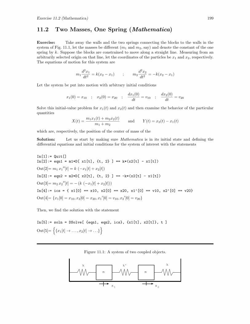
Exercise 11.2 (Mathematica) 199
11.2 Two Masses, One Spring (Mathematica)
Exercise: Take away the walls and the two springs connecting the blocks to the walls in thesystem of Fig. 11.1, let the masses be different (m1 and m2, say) and denote the constant of the onespring by k. Suppose the blocks are constrained to move along a straight line. Measuring from anarbitrarily selected origin on that line, let the coordinates of the particles be x1 and x2, respectively.The equations of motion for this system are
m1d2x1
dt2= k(x2 − x1) ; m2
d2x2
dt2= −k(x2 − x1)
Let the system be put into motion with arbitrary initial conditions
x1(0) = x10 ; x2(0) = x20 ;dx1(0)
dt= v10 ;
dx2(0)
dt= v20
Solve this initial-value problem for x1(t) and x2(t) and then examine the behavior of the particularquantities
X(t) =m1x1(t) +m2x2(t)
m1 +m2and Y (t) = x2(t)− x1(t)
which are, respectively, the position of the center of mass of the
Solution: Let us start by making sure Mathematica is in its initial state and defining thedifferential equations and initial conditions for the system of interest with the statements
In[1]:= Quit[]
In[2]:= eqn1 = m1*D[ x1[t], t, 2 ] == k*(x2[t] - x1[t])
Out[2]= m1 x1′′[t] = k (−x1[t] + x2[t])
In[3]:= eqn2 = m2*D[ x2[t], t, 2 ] == -k*(x2[t] - x1[t])
Out[3]= m2 x2′′[t] = − (k (−x1[t] + x2[t]))
In[4]:= ics = x1[0] == x10, x2[0] == x20, x1’[0] == v10, x2’[0] == v20
Out[4]= x1[0] = x10, x2[0] = x20, x1′[0] = v10, x2
′[0] = v20
Then, we find the solution with the statement
In[5]:= soln = DSolve[ eqn1, eqn2, ics, x1[t], x2[t], t ]
Out[5]=x1[t]→ . . . , x2[t]→ . . .
Figure 11.1: A system of two coupled objects.
m m
k k’ k
x1 x2
200 Exercise 11.2 (Mathematica)
where, of course, the ellipses stand for the actual (elaborate and extensive) expressions that Mathe-matica supplies. The resulting expressions, however, include some terms that vary sinusoidally withthe frequency
Ω =
√km2
2m1 + km2m21
m2m1=
√km1 +m2
m1m2=
√k
(1
m1+
1
m2
)=
√k
mred
where mred, defined by1
mred=
1
m1+
1
m2or mred =
m1m2
m1 +m2
is called the reduced mass of the two-body system. With this recognition, we can simplify theappearance of the solution by substituting Ω for the frequency. First, we must transform theexponential solution that Mathematica gives us to the trigonometric solution. To accomplish thistransformation we execute the statements
In[6]:= soln1 = soln[[1]][[1]][[2]], soln[[1]][[2]][[2]] ;
In[7]:= soln2 = soln1 /. Sqrt[-k*m1^2*m2 - k*m1*m2^2] ->
I*Sqrt[k*m2^2*m1 + k*m2*m1^2]
In[8]:= soln3 = ExpToTrig[soln2];
In these statements, we first form a list of just the actual solutions found by DSolve. This stepis needed so that the ExpToTrig function can be applied later. Then we perform a substitutionto make Mathematica realize the presence of imaginary numbers. After this step we perform thetransformation from exponential to trigonometric form. Finally, we perform the desired substitutionand reassign these values to x1[t] and x2[t] with the statements
In[9]:= soln4 = soln3 /. Sqrt[k*m2^2*m1 + k*m2*m1^2] ->
m2*m1*\[CapitalOmega];
In[10]:= soln5 = x1[t] -> soln4[[1]], x2[t] -> soln4[[2]] ;
Then, without worrying about which order x1[t] and x2[t] are presented, we can extract the solutionfor x1[t] as an expression with the statement
In[11]:= x1 = Simplify[ Evaluate[x1[t] /. soln5] ]
Out[11]=
m1m2
((m1tΩ +m2 sin(tΩ))v10 +m2(tΩ− sin(tΩ)) v20
+Ω( (m1 +m2 cos(tΩ))x10 −m2(−1 + cos(tΩ))x20 ))
(m1 +m2)√−km1m2(m1 +m2)
and we can extract the solution for x2[t] with the statement
In[12]:= x2 = Simplify[ Evaluate[x2[t] /. soln5] ]
Out[12]=
m1m2
(m1(tΩ− sin(tΩ)) v10 + (m2tΩ +m1 sin(tΩ)) v20
+Ω( (m1 −m1 cos(tΩ))x10 + (m2 +m1 cos(tΩ))x20 ))
(m1 +m2)√−km1m2 (m1 +m2)
Exercise 11.2 (Mathematica) 201
Now, for some reason, the above operation that substituted Ω for the frequency in some of theterms failed to find and replace the square roots in the denominators of some of the terms. Effectingthat replacement (and simplification) appears to require more involved manipulation. For x1, forexample, we can with the statement
In[13]:= den = Part[ x1[[1]], 5 ]
Out[13]=1√
−km1m2(m1 +m2)
confirm that the fifth part of the first element in x1 is the reciprocal of the square root we seek toreplace.2 Then, we can replace that operand with the equivalent expression 1/(m2m1Ω)i with thestatement
In[14]:= x1 = x1 /. Part[ x1[[1]], 5 ] -> 1/(I*\[CapitalOmega]*m1*m2)
Out[14]=
(m1tΩ +m2 sin(tΩ))v10 +m2(tΩ− sin(tΩ))v20
+Ω(
(m1 +m2 cos(tΩ))x10 −m2(−1 + cos(tΩ))x20
)(m1 +m2)Ω
Now we simplify this expression by executing the statements
In[15]:= x1 = Expand[x1];
In[16]:= x1 = Collect[ x1, \[CapitalOmega], t, Sin[t*\[CapitalOmega] ],
Cos[t*\[CapitalOmega]], m1 + m2 , m2]
Out[16]=
m2 sin(tΩ) (v10 − v20)
(m1 +m2)Ω+t(m1v10 +m2v20)
m1 +m2
+m2 cos(tΩ) (x10 − x20)
m1 +m2+m1x10 +m2x20
m1 +m2
Similarly, with the statement
In[17]:= den2 = Part[ x2[[1]], 5 ]
Out[17]=1√
−km1m2(m1 +m2)
we confirm that the fifth part of the first part in x2 is the reciprocal of the square root we seek toreplace.3 Then, we can replace that operand with the equivalent expression 1/(m2m1Ω)i with thestatement
In[18]:= x2 = x2 /. Part[ x2[[1]], 5 ] -> 1/(I*\[CapitalOmega]*m1*m2)
Out[18]=
m1(tΩ− sin(tΩ))v10 + (m2tΩ +m1 sin(tΩ))v20
+Ω(
(m1 −m1 cos(tΩ))x10 + (m2 +m1 cos(tΩ))x20
)(m1 +m2)Ω
2The position of this operand in your expression may not be the same as here. Thus, you may have to experiment
a bit to find the proper location for your session with Mathematica.3See the previous footnote.
202 Exercise 11.2 (Mathematica)
Now we simplify this expression by executing the statements
In[19]:= x2 = Expand[x2]
In[20]:= x2 = Collect[ x2, \[CapitalOmega], t, Sin[t*\[CapitalOmega] ],
Cos[t*\[CapitalOmega]], m1 + m2, m1 ]
Out[20]=
m1 sin(tΩ) (−v10 + v20)
(m1 +m2) Ω+t (m1v10 +m2 v20)
m1 +m2
+m1 cos(tΩ) (−x10 + x20)
m1 +m2+m1x10 +m2x20
m1 +m2
These results are now probably about as simple as we can make them, so we will stop at this pointwith efforts to recast them.
Now, we are ready to look at the center of mass of the system, X(t), as well as the position ofthe second block relative to the first, Y (t). To find the center of mass, we invoke the statements
In[21]:= X = Simplify[ (m1*x1 + m2*x2)/(m1 + m2) ]
Out[21]=
m1tv10 +m2tv20 +m1x10 +m2x20
m1 +m2
In[22]:= X=Collect[ X, t ]
Out[22]=
t (m1v10 +m2v20)
m1 +m2+m1x10 +m2x20
m1 +m2
This interesting result has the simple form X = X0 + Vcmt, where
X0 =m1x10 +m2x20
m1 +m2; Vcm =
m1v10 +m2v20
m1 +m2
In other words, the center of mass of the moving system starts at the initial position of the center ofmass and moves along a straight line at constant velocity Vcm. This result, of course, confirms ourexpectation that, in the absence of external forces, the linear momentum of the composite systemmust be conserved. However, as the spring stretches and contracts, the center of mass will motoralong at a constant velocity. Note also that the velocity of the center of mass is independent of thespring constant.
To find the motion of the second object relative to the first, we would use instead the Mathe-matica statements
In[23]:= Y = Expand[ Simplify[x2 - x1] ];
Out[23]=
−(
sin(tΩ) v10
Ω
)+
sin(tΩ) v20
Ω− cos(tΩ)x10 + cos(tΩ)x20
In[24]:= Y = Collect[ Y, Sin[t*\[CapitalOmega]], Cos[t*\[CapitalOmega] ] ]
Out[24]=
sin(tΩ)(−(v10
Ω
)+v20
Ω
)+ cos(tΩ) (−x10 + x20)
Since the coefficients of the sine and cosine terms are constants, this expression for Y (t) can begeneralized as A cos(Ωt) + B sin(Ωt). We conclude, then that the motion of the second objectrelative to the first is simple harmonic and is given by an oscillating function that could, if we chose,be written as a single sinusoidal function with an appropriate amplitude and phase. The mainpoint is that the separation of the two objects oscillates quite simply as the two objects individuallymove closer to and further away from the equilibrium position (so long, of course, as we remain in

Exercise 11.2 (Mathematica) 203
our frictionless dreamworld). Note that, in terms of the reduced mass mred, the frequency of theoscillation has the simple relationship
Ω =
√k
mred
to the parameters describing the system. Indeed, the relative motion is identical to that of a singleobject of mass mred on a spring of constant k.
Taken together, then, we have a system of two blocks moving across a surface, with the center ofmass moving at constant velocity, and, as the motion ensues, with m2 pulling m1, then m1 catchingup and pushing block m2, then . . .. This pushing and pulling process is repeated indefinitely. Thebehavior, of course, follows directly from the forces and Newton’s laws of motion.
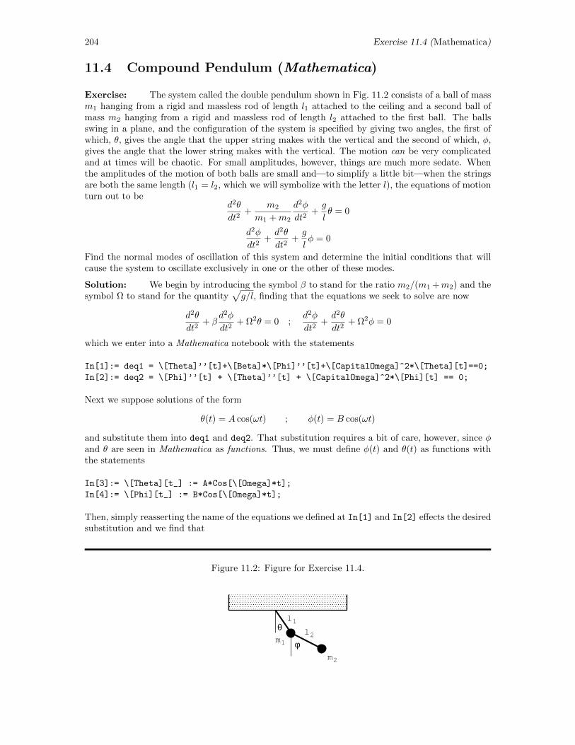
204 Exercise 11.4 (Mathematica)
11.4 Compound Pendulum (Mathematica)
Exercise: The system called the double pendulum shown in Fig. 11.2 consists of a ball of massm1 hanging from a rigid and massless rod of length l1 attached to the ceiling and a second ball ofmass m2 hanging from a rigid and massless rod of length l2 attached to the first ball. The ballsswing in a plane, and the configuration of the system is specified by giving two angles, the first ofwhich, θ, gives the angle that the upper string makes with the vertical and the second of which, φ,gives the angle that the lower string makes with the vertical. The motion can be very complicatedand at times will be chaotic. For small amplitudes, however, things are much more sedate. Whenthe amplitudes of the motion of both balls are small and—to simplify a little bit—when the stringsare both the same length (l1 = l2, which we will symbolize with the letter l), the equations of motionturn out to be
d2θ
dt2+
m2
m1 +m2
d2φ
dt2+g
lθ = 0
d2φ
dt2+d2θ
dt2+g
lφ = 0
Find the normal modes of oscillation of this system and determine the initial conditions that willcause the system to oscillate exclusively in one or the other of these modes.
Solution: We begin by introducing the symbol β to stand for the ratio m2/(m1 +m2) and thesymbol Ω to stand for the quantity
√g/l, finding that the equations we seek to solve are now
d2θ
dt2+ β
d2φ
dt2+ Ω2θ = 0 ;
d2φ
dt2+d2θ
dt2+ Ω2φ = 0
which we enter into a Mathematica notebook with the statements
In[1]:= deq1 = \[Theta]’’[t]+\[Beta]*\[Phi]’’[t]+\[CapitalOmega]^2*\[Theta][t]==0;
In[2]:= deq2 = \[Phi]’’[t] + \[Theta]’’[t] + \[CapitalOmega]^2*\[Phi][t] == 0;
Next we suppose solutions of the form
θ(t) = A cos(ωt) ; φ(t) = B cos(ωt)
and substitute them into deq1 and deq2. That substitution requires a bit of care, however, since φand θ are seen in Mathematica as functions. Thus, we must define φ(t) and θ(t) as functions withthe statements
In[3]:= \[Theta][t_] := A*Cos[\[Omega]*t];
In[4]:= \[Phi][t_] := B*Cos[\[Omega]*t];
Then, simply reasserting the name of the equations we defined at In[1] and In[2] effects the desiredsubstitution and we find that
Figure 11.2: Figure for Exercise 11.4.
θ
φ
l1l2
m1
m2
Exercise 11.4 (Mathematica) 205
In[5]:= eq1 = deq1
Out[5]= −Aω2 Cos [tω]−Bβω2 Cos [tω] +AΩ2 Cos [tω] == 0
In[6]:= eq2 = deq2
Out[6]= −Aω2 Cos [tω]−Bω2 Cos [tω] +BΩ2 Cos [tω] == 0
Then, dividing out the factor cos(ωt) with the statements
In[7]:= eq3 = Simplify[eq1[[1]]/Cos[\[Omega]*t]] == 0
Out[7]= −Bβω2 +A(−ω2 + Ω2) == 0
In[8]:= eq4 = Simplify[eq2[[1]]/Cos[\[Omega]*t]] == 0
Out[8]= −Aω2 +B(−ω2 + Ω2) == 0
we arrive at two algebraic equations (eq3 and eq4), for which we seek conditions under whichnon-trivial solutions for A and B can be found. Writing these two equations in the form(
−ω2 + Ω2 −βω2
−ω2 −ω2 + Ω2
)(AB
)=
(00
)we see that, in essence, we want to extract the coefficient matrix with respect to the constants(A,B) and then find the values of ω2 which will cause the determinant of that matrix to be zero.The statements
In[9]:= << LinearAlgebra‘MatrixManipulation‘
In[10]:= tmp = LinearEquationsToMatrices[eq3, eq4, A, B][[1]];
In[11]:= MatrixForm[tmp]
Out[11]=
(−ω2 + Ω2 −βω2
−ω2 −ω2 + Ω2
)
will extract the coefficient matrix. Then, the statement
In[12]:= detm = Expand[ Det[tmp] ]
Out[12]= ω4 − βω4 − 2ω2Ω2 + Ω4
finds the determinant, the statement
In[13]:= det1 = detm /. \[Omega] -> Sqrt[ \[Alpha] ]
Out[13]= α2 − βα2 − 2αΩ2 + Ω4
temporarily replaces ω2 with α so Mathematica will recognize the expression as a quadratic equation(in α). the statement
In[14]:= soln = Solve[ det1 == 0, \[Alpha] ]
Out[14]=
α→ − Ω2
−1 +√β
,α→ Ω2
1 +√β
generates the two solutions for α, and—at last—-the statements
206 Exercise 11.4 (Mathematica)
In[15]:= w1 = Sqrt[ \[Alpha] ] /. soln[[1]]
Out[15]=
√− Ω2
−1 +√β
In[16]:= w2 = Sqrt[ \[Alpha] ] /. soln[[2]]
Out[16]=
√Ω2
1 +√β
yield the two separate solutions for ω. (We don’t bother with the negative square roots, since thesign of ω is irrelevant to the solution. Further, we note that 0 ≤ β ≤ 1 and the quantities underthe square roots are therefore always positive; the solutions indeed are oscillatory, not exponentiallygrowing or decaying.)
We must, however, also find the initial amplitudes that will start the system oscillating inthe normal mode corresponding to each of these frequencies. To do so, we return to the algebraicequations eq3 and eq4. We set ω in eq3 to w1 and solve for B—denote it B1—as a multiple of Awith the statements
In[17]:= Simplify[ eq3 /. \[Omega] -> w1 ];
In[18]:= B1 = Solve[%, B][[1,1]]
Out[18]= B → − A√β
Then, we verify that eq4 is satisfied as well with the statement
In[19]:= Simplify[ eq4 /. B1, \[Omega] -> w1 ]
Out[15]= True
Parallel statements applied to the second frequency yield the results
In[20]:= Simplify[ eq3 /. \[Omega] -> w2 ];
In[21]:= B2 = Solve[%, B][[1,1]]
Out[21]= B → A√β
Int[22]:= Simplify[eq4 /. B2, \[Omega] -> w2 ]
Out[22]= True
Intriguingly, one normal mode is obtained by displacing the upper pendulum by some amountA in one direction and the lower pendulum by an amount A/
√β—which is larger than A because
β < 1—in the same direction, while the other normal mode is obtained by displacing the upperpendulum by some amount A in one direction and the lower pendulum by an amount A/
√β in the
other direction. The interesting feature is that the displacement of the second pendulum in the twocases has the same magnitude even though the direction is different. In both cases the pendula arereleased from rest.
We should note also that the mode in which the two pendula are displaced in the same directionwill oscillate with the frequency
ω1 =Ω√
1−√β
=
√g/l√
1−√β

Exercise 11.4 (Mathematica) 207
while the mode in which the two pendula are displaced in opposite directions will oscillate with thefrequency
ω2 =Ω√
1 +√β
=
√g/l√
1 +√β
From these relationships, we note that ω2 < ω1. As we would expect (and as has turned out to bethe case, the mode in which the pendula oscillate in phase would be the lower frequency mode andthe mode in which the pendula oscillate out of phase would be the higher frequency mode. Notealso that the unit
√g/l in which these frequencies are expressed is the frequency of small amplitude
oscillations of a single pendulum of length l.
208 Exercise 11.6 (Mathematica)
11.6 Series Solution (Mathematica)
Exercise: Among the simplest of differential equations is the equation
d2x
dt2+ ω2x = 0
that describes a simple harmonic oscillator. Generate a series solution to this equation and thenverify that the solution thus generated agrees with the known solution
x(t) = A cosωt+B sinωt
where A and B are constants determined by the initial conditions.
Solution: Solving differential equations using series in Mathematica is easy if one knows theright statements. We begin by assigning the left-hand side of the differential equation
d2x
dt2+ ω2x = 0
to the variable eq1 with the statement
In[1]:= eq1 = D[x[t], t, 2] + \[Omega]^2*x[t]
Out[1]= ω2 x[t] + x′′[t]
Now, supposing a solution of the form
x(t) =
∞∑i
aiti+γ
we create a (truncated) series with the statement
In[2]:= x[t_] := Sum[ a[i]*t^(i+\[Gamma]), i, 0, 10 ]
Then, we substitute this expression into the differential equation with the statement
In[3] := ode = eq1
Out[3]= (result too long to record)
Each term in this result, however, has a factor of tγ , which we can remove by division. To simplifythe expression, we also multiply by t2, which adjusts every power of t upward by 2 and creates anexpression in which the lowest power of t is t0. (We can perform these adjustments because theresult is set equal to zero. Since t is not identically zero, we can multiply the overall expression by tto any power without destroying the “zero-ness” of the result.) Thus, we we invoke the statements
In[4]:= soln1 = Expand[ t^2*ode/t^\[Gamma] ];
In[5]:= soln2 = Collect[ soln1, t ]
Out[5]= −γa0 + γ2a0 + t(γa1 + γ2a1) + t2(ω2a0 + 2a2 + 3γa2 + γ2a2) + . . .
Following the pattern in Section 9.5.8, we now extract the coefficients with the statement
In[6]::= coefs = CoefficientList[ soln2, t ]
Out[6]= −γa0 + γ2a0, (γa1 + γ2a1), (ω2a0 + 2a2 + 3γa2 + γ2a2), . . .
Exercise 11.6 (Mathematica) 209
Each coefficient in this list must itself be zero. To find the possible values of γ, we require the firstcoefficient to be zero, discovering with the statement
In[7]:= gam = Solve[ coefs[[1]]==0, \[Gamma] ]
Out[7]= γ → 0, γ → 1
that γ can be either 0 or 1. (We assume that a0 6= 0.)
Suppose we take γ = 1 first. To find the coefficients in this case, we would execute the statements
In[8]:= coefs1 = coefs /. gam[[2]]
Out[8]= 0, 2a1, ω2a0 + 6a2, ω
2a1 + 12a3, ω2a2 + 20a4, ω
2a3 + 30a5, ω2a4 + 42a6, ω
2a5 + 56a7,
ω2a6 + 72a8, ω2a7 + 90a9, ω
2a8 + 110a10, ω2a9, ω
2a10
In[9]:= eqs1 = Table[ coefs1[[i+1]]==0, i, 10 ]
Out[9]= 2a1 == 0, ω2a0 + 6a2 == 0, ω2a1 + 12a3 == 0, ω2a2 + 20a4 == 0,
ω2a3 + 30a5 == 0, ω2a4 + 42a6 == 0, ω2a5 + 56a7 == 0,
ω2a6 + 72a8 == 0, ω2a7 + 90a9 == 0, ω2a8 + 110a10 == 0
In[10]:= vars1 = Table[ a[i], i, 10 ]
Out[10]= a1, a2, a3, . . . , a10
In[11]:= Solve[ eqs1, vars1 ][[1]]
Out[11]=
a9 → 0, a10 → −
ω10
39916800a0, a1 → 0, a2 → −
ω2
6a0, a3 → 0, a4 →
ω4
120a0,
a5 → 0, a7 → 0, a6 → −ω6
5040a0, a8 →
ω8
362880a0
(At In[9], we ignore the first coefficient, which is already zero, and we ignore the last two, whichare incomplete because of the truncation of the series.) Then, we obtain the series for the solutioncorresponding to γ = 1, we execute the statements
In[12]:= x[t] /. \[Gamma]->1;
In[13]:= % /. %11;
In[14]:= soln3 = Collect[ %, a[0] ]
Out[14]=
(t− t3ω2
6+t5ω4
120− t7ω6
5040+
t9ω8
362880− t11ω10
39916800
)a0
If we now recognize that 3! = 6, 5! = 120, 7! = 5040, 9! = 362880, and 11! = 39916800 and alsomultiply and divide by ω, we can recast this result as the series
a0
ω
(ωt− t3ω3
6+t5ω5
120− t7ω7
5040+
t9ω9
362880− t11ω11
39916800
)which we recognize as the beginning of the series for
a0
ωsin(ωt)
though we need not come to that recognition for the series solution to be valid or useful in its ownright.
The solution when γ = 0 can be found in a similar way. We begin by finding the coefficientswhen γ = 0 with the statement
210 Exercise 11.6 (Mathematica)
In[15]:= coefs0 = coefs /. gam[[1]]
Out[15]= 0, 0, ω2a0 + 2a2, ω2a1 + 6a3, ω
2a2 + 12a4, ω2a3 + 20a5, ω
2a4 + 30a6, ω2a5 + 42a7,
ω2a6 + 56a8, ω2a7 + 72a9, ω
2a8 + 90a10, ω2a9ω
2a10
Each of these coefficients must itself be zero, a property whose consequences we explore with thestatements
In[16]:= eqs0 = Table[ coefs0[[i+2]]==0, i, 9 ]
Out[16]= ω2a0 + 2a2 == 0, ω2a1 + 6a3 == 0, ω2a2 + 12a4 == 0,
ω2a3 + 20a5 == 0, ω2a4 + 30a6 == 0, ω2a5 + 42a7 == 0,
ω2a6 + 56a8 == 0, ω2a7 + 72a9 == 0, ω2a8 + 90a10 == 0
In[17]:= vars0 = Table[ a[i+1], i, 9 ]
Out[17]= a2, a3, a4, a5, a6, a7, a8, a9, a10
In[18]:= Solve[ eqs0, vars0 ][[1]]
Out[18]=
a9 →
ω8
362880a1, a10 →
ω10
3628800a1, a2 → −
ω2
2a1, a4 →
ω4
24a1, a6 → −
ω6
720a1,
a8 →ω8
40320a1, a7 → −
ω6
5040a1, a5 →
ω4
120a1, a3 → −
ω2
6a1
Neither a0 nor a1 is fixed by these conditions. Finally, substituting these solutions into the serieswith which we began, we find that
In[19]:= x[t] /. \[Gamma]->0;
In[20]:= % /. %18;
In[21]:= Collect[ %, a[0], a[1] ]
Out[21]=
(1− ω2t2
2+ω4t4
24− ω6t6
720+
ω8t8
40320− ω10t10
3628800
)a0
+
(t− ω2t3
6+ω4t5
120− ω6t7
5040+
ω8t9
362880
)a1
As above, the series involving odd powers of t can be recognized as the beginning several terms inthe Taylor expansion of sin(ωt). Recognizing that 4! = 24, 6! = 720, 8! = 40320, and 10! = 3628800,we similarly recognize the series involving even powsrs of t as the beginnings of the Taylor expansionof cos(ωt). Based on these observations, we infer that the solution we have obtained by applyingthe method of Frobenius is consistent with the aolution
x(t) = a0 cos(ωt) +a1
ωsin(ωt)
Finally, we want to compare the (truncated) series with the analytic solution, i.e., we want tocompare
xseries(t) =
(1− ω2t2
2+ω4t4
24− ω6t6
720+
ω8t8
40320− ω10t10
3628800
)a0
+
(t− ω2t3
6+ω4t5
120− ω6t7
5040+
ω8t9
362880
)a1
withxanalytic(t) = a0 cos(ωt) +
a1
ωsin(ωt)
We define the necessary expressions with the statements
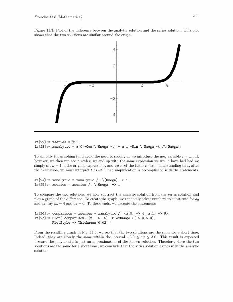
Exercise 11.6 (Mathematica) 211
Figure 11.3: Plot of the difference between the analytic solution and the series solution. This plotshows that the two solutions are similar around the origin.
-4 -2 2 4
-4
-2
2
4
In[22]:= xseries = %21;
In[23]:= xanalytic = a[0]*Cos[\[Omega]*t] + a[1]*Sin[\[Omega]*t]/\[Omega];
To simplify the graphing (and avoid the need to specify ω, we introduce the new variable τ = ωt. If,however, we then replace τ with t, we end up with the same expression we would have had had wesimply set ω = 1 in the original expressions, and we elect the latter course, understanding that, afterthe evaluation, we must interpret t as ωt. That simplification is accomplished with the statements
In[24]:= xanalytic = xanalytic /. \[Omega] -> 1;
In[25]:= xseries = xseries /. \[Omega] -> 1;
To compare the two solutions, we now subtract the analytic solution from the series solution andplot a graph of the difference. To create the graph, we randomly select numbers to substitute for a0
and a1, say a0 = 4 and a1 = 6. To these ends, we execute the statements
In[26]:= comparison = xseries - xanalytic /. a[0] -> 4, a[1] -> 6;
In[27]:= Plot[ comparison, t, -5, 5, PlotRange->-5.0,5.0,
PlotStyle -> Thickness[0.02] ]
From the resulting graph in Fig. 11.3, we see that the two solutions are the same for a short time.Indeed, they are closely the same within the interval −3.0 ≤ ωt ≤ 3.0. This result is expectedbecause the polynomial is just an approximation of the known solution. Therefore, since the twosolutions are the same for a short time, we conclude that the series solution agrees with the analyticsolution.
212 Exercise 11.7 (Mathematica)
11.7 Projectile in Linear Air Resistance (Mathematica)
Exercise: Find a symbolic solution for all three components for the motion of a projectile ina linear, viscous medium, when the initial conditions are general, i.e., solve the equations
md2x
dt2= −bdx
dt; m
d2y
dt2= −bdy
dt; m
d2z
dt2= −mg − bdz
dt
subject to the initial conditions
x(0) = x0 ; y(0) = y0 ; z(0) = 0 ;dx
dt(0) = vx0 ;
dy
dt(0) = vy0 ;
dz
dt(0) = vz0
Since the equations are uncoupled, you can solve each individually. Alternatively, you can solve thethree equations simultaneously as a system. Solve them both ways. Once you have the solutionsin hand, verify that they satisfy the original equations and initial conditions. Finally, explore theirlimits for small b.
Solution: The problem defined by the differential equations and the initial conditions above isfairly straightforward. We simply define the equations, solve them, and determine the integrationconstants to match the initial conditions. Appropriate statements to Mathematica are
In[1]:=
Out[1]= mx′′[t] == −b x′[t]
In[2]:= eqdy = m*y’’[t] == -b*y’[t]
Out[2]= my′′[t] == −b y′[t]
In[3]:= eqdz = m*z’’[t] == -m*g -b*z’[t]
Out[3]= mz′′[t] == −gm− b z′[t]
In[4]:= solnx = DSolve[ eqdx, x[0]==x0, x’[0]==vx0, x, t ]
Out[4]= x→ Function[t, . . .]
In[5]:= solnx1 = x[t] /. solnx;
In[6]:= solnx1 = solnx1[[1]];
In[7]:= solnx1 = Collect[ Expand[solnx1], m*vx0/b ]
Out[7]= :=1− e−bt/mmvx0
b+ x0
In[8]:= solny = DSolve[ eqdy, y[0]==y0, y’[0]==vy0, y, t ]
Out[4]= y → Function[t, . . .]
In[9]:= solny1 = y[t] /. solny;
In[10]:= solny1 = solny1[[1]];
In[11]:= solny1 = Collect[ Expand[solny1], m*vy0/b ]
Out[11]= :=1− e−bt/mmvy0
b+ y0
In[12]:= solnz = DSolve[ eqdz, z[0]==z0, z’[0]==vz0, z, t ]
Out[12]= z → Function[t, . . .]
In[12]:= solnz1 = z[t] /. solnz;
In[13]:= solnz1 = solnz1[[1]];
Exercise 11.7 (Mathematica) 213
In[14]:= solnz1 = Collect[ Expand[solnz1], Exp[-b*t/m] ]
Out[14]=gm2
b2− gmt
b+mvz0b
+ e−bt/m(−gm
2
b2− mvz0
b
)+ z0
Alternatively, we can solve all three of the equations at once with the Mathematica statements
In[15]:= soln = DSolve[ eqdx, eqdy, eqdz, x[0]==x0, x’[0]==vx0,
y[0]==y0, y’[0]==vy0, z[0]==z0, z’[0]==vz0,
x, y, z , t ]
which yields output having the form
Out[15]= x→ Function[t, . . .], y → Function[t, . . .], z → Function[t, . . .]
where the three solutions are identical to those obtained separately in the first calculation. Then,we could extract the separate solutions with the statements
In[16]:= solnx2 = x[t] /. soln;
In[17]:= solny2 = y[t] /. soln;
In[18]:= solnz2 = z[t] /. soln;
and manipulate these entities in the same way as above to obtain the same final solutions.
To verify that each solution satisfies the original equation, we would invoke the Mathematicastatements
In[19]:= Simplify[ eqdx /. solnx[[1]] ]
Out[19]= TrueIn[20]:= Simplify[ eqdy /. solny[[1]] ]
Out[20]= TrueIn[21]:= Simplify[ eqdz /. solnz[[1]] ]
Out[21]= True
Further, we can verify the satisfaction of the initial conditions by invoking the statements
In[22]:= Simplify[ x[0], x’[0] /. solnx[[1]] ]
Out[22]= x0, vx0In[23]:= Simplify[ y[0], y’[0] /. solny[[1]] ]
Out[23]= y0, vy0In[24]:= Simplify[ z[0], z’[0] /. solnz[[1]] ]
Out[24]= z0, vz0
Finally, to determine the behavior of the solutions x(t), y(t), and z(t) for small b, we evaluateTaylor series, going far enough (after some trial) to include the terms of order b2. We find that
In[25]:= Series[ solnx1, b, 0, 2 ]
Out[25]= (x0 + vx0t)−vx0t
2
2mb+
vx0t3
6m2b2 +O[b]3
In[26]:= Series[ solny1, b, 0, 2 ]
Out[26]= (y0 + vy0t)−vy0t
2
2mb+
vy0t3
6m2b2 +O[b]3
In[27]:= Simplify[ Series[ solnz1, b, 0, 2 ] ]
Out[27]=
(−gt
2
2+ tvz0 + z0
)+t2(gt− 3vz0)
6mb− t3(gt− 4vz0)
24m2+O[b]3
The zeroth-order terms, of course, agree with what we would expect in the absence of air resistance.
214 Exercise 11.12 (MATHEMATICA)
11.12 Vibrating String Fixed at Both Ends (MATHEMAT-ICA)
Exercise: In an appropriate dimensionless presentation, standing waves in a string must satisfythe boundary value problem
d2y
dx2+ k2y = 0 ; y(0) = y(1) = 0
Suppose that the interval 0 ≤ x ≤ 1 is divided into n equal segments of length ∆x = 1/n, letxi = i∆x (with i = 0, 1, 2, . . . , n), and let yi = y(xi). Evaluate the ODE at x = xi, approximate thesecond derivative with the difference formula
d2y
dx2
∣∣∣∣x=xi
≈ yi+1 − 2yi + yi−1
∆x2; i = 1, 2, 3, . . . n− 1
and note that y0 = yn = 0. Show that the values yi for i = 0, 1, 2, . . . , n satisfy a system of n+1 linearalgebraic equations of the form M Y = αY , where Y is an (n+1)-component vector whose elementsare the values of yi and α is determined from k2 and ∆x. Then argue that the allowed values of k2
can be determined from the eigenvalues of the matrix M . That is, show that this transformationturns a boundary value problem involving a differential equation into an approximately equivalentmatrix eigenvalue problem.
Solution: Since the string is fixed at x = 0 and x = 1, we cannot use Euler’s method or a moresophisticated method to address this exercise. Instead, we must divide the interval 0 ≤ x ≤ 1 into nequal segments of length ∆x = 1/n. Then using, xi = i∆x and yi = y(xi) (where i = 0, 1, 2, . . . , n),we use the formula in the second equation in the statement of the exercise to approximate the secondderivative and seek to solve the family of equations
yi+1 − 2yi + yi−1
∆x2= −k2yi
To illustrate the procedure, we suppose n = 4, but the process is similar for other values of n. InMATHEMATICA, the statements 4
In[1]:= eqs = Array[eq,5]
Out[1]= eq[1], eq[2], eq[3], eq[4], eq[5]
In[[2]]:= eqs[[1]] = y[1] == 0;
In[[3]]:= eqs[[5]] = y[5] == 0;
In[[4]]:= For[ i=2,i<=4,i++, eqs[[i]] = y[i+1]-2*y[i]+y[i-1] == -k^2*d^2*y[i] ]
In[5]:= eqs
Out[5]= y[1] == 0,
y[1] - 2 y[2] + y[3] == -d^2 k^2 y[2],
y[2] - 2 y[3] + y[4] == -d^2 k^2 y[3],
y[3] - 2 y[4] + y[5] == -d^2 k^2 y[4],
y[5] == 0
In[6]:= eqs = eqs/. y[1]->0, y[5]->0
Out[6]= True,
- 2 y[2] + y[3] == -d^2 k^2 y[2],
y[2] - 2 y[3] + y[4] == -d^2 k^2 y[3],
y[3] - 2 y[4] == -d^2 k^2 y[4],
True
In[7]:= eqss = Delete[ eqs, 1, 5 ]
Out[7]= - 2 y[2] + y[3] == -d^2 k^2 y[2],
y[2] - 2 y[3] + y[4] == -d^2 k^2 y[3],
y[3] - 2 y[4] == -d^2 k^2 y[4]
4For simplicity in notation, we use d instead of δx in this coding.
Exercise 11.12 (MATHEMATICA) 215
yielding three equations in the form My = −k2d2y where y is the vector [y1, y2, y3] and M is thecoefficient matrix for the system of the three linear equations for the components of y. Specifically,−k2d2 is an eigenvalue of the coefficient matrix M , which is readily extracted with the statements
In[8]:= For[ i = 1, i <= 3, i++, eqss[[i]] = eqss[[i, 1]] ]
In[9]:= eqss
Out[9]= -2 y[2] + y[3],
y[2] - 2 y[3] + y[4],
y[3] - 2 y[4]
In[10]:= yy = Delete[ Array[y, 5], 1, 5]
Out[10]= y[2], y[3], y[4]
In[11]:= M = Normal[ CoefficientArrays[ eqss, yy ] ]
Out[11]= 0, 0, 0, -2, 1, 0, 1, -2, 1, 0, 1, -2
In[12]:= M = M[[2]]
Out[12]= -2, 1, 0, 1, -2, 1, 0, 1, -2
In[13]:= MatrixForm[%]
Out[13]//MatrixForm=
−2 1 01 −2 10 1 −2
Non-trivial solutions for the system of three equations at Out[7] can be found only if −d2k2 hasone of the three eigenvalues of this 3× 3 matrix so the acceptable values of k are given by
In[14]:= evals = Eigenvalues[ M ]
Out[14]= −2−√
2,−2,−2 +√
2
In[15]:= vals = N[ evals ]
Out[15]= -3.41421, -2., -0.585786
Finally, since the eigenvalues are values of −k2d2, the acceptable values of k are found with thestatements
In[16]:= Assuming[d>0, Map[ FullSimplify[ Map[Sqrt,-vals/d^2]] ] ]
Out[16]= Map[ 1.84776/d, 1.41421.d, 0.765367/d ]
The same procedures can be implemented for much larger values of n to achieve a more accuratedetermination of the eigenvalues
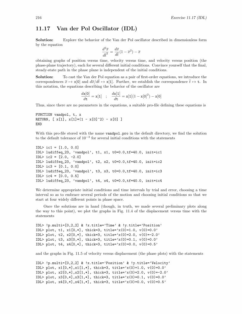
216 Exercise 11.17 (IDL)
11.17 Van der Pol Oscillator (IDL)
Solution: Explore the behavior of the Van der Pol oscillator described in dimensionless formby the equation
d2x
dt2 =
dx
dt(1− x2)− x
obtaining graphs of position versus time, velocity versus time, and velocity versus position (thephase-plane trajectory), each for several different initial conditions. Convince yourself that the final,steady-state path in the phase plane is independent of the initial conditions.
Solution: To cast the Van der Pol equation as a pair of first-order equations, we introduce thecorrespondences x 7→ x[0] and dx/dt 7→ x[1]. Further, we establish the correspondence t 7→ t. Inthis notation, the equations describing the behavior of the oscillator are
dx[0]
dt= x[1] ;
dx[1]
dt= x[1](1− x[0]
2)− x[0]
Thus, since there are no parameters in the equations, a suitable pro-file defining these equations is
FUNCTION vandpol, t, x
RETURN, [ x[1], x[1]*(1 - x[0]^2) - x[0] ]
END
With this pro-file stored with the name vandpol.pro in the default directory, we find the solutionto the default tolerance of 10−3 for several initial conditions with the statements
IDL> ic1 = [1.0, 0.0]
IDL> ludiffeq_23, ’vandpol’, t1, x1, t0=0.0,tf=40.0, init=ic1
IDL> ic2 = [2.0, -2.0]
IDL> ludiffeq_23, ’vandpol’, t2, x2, t0=0.0,tf=40.0, init=ic2
IDL> ic3 = [0.1, 0.0]
IDL> ludiffeq_23, ’vandpol’, t3, x3, t0=0.0,tf=40.0, init=ic3
IDL> ic4 = [0.0, 0.5]
IDL> ludiffeq_23, ’vandpol’, t4, x4, t0=0.0,tf=40.0, init=ic4
We determine appropriate initial conditions and time intervals by trial and error, choosing a timeinterval so as to embrace several periods of the motion and choosing initial conditions so that westart at four widely different points in phase space.
Once the solutions are in hand (though, in truth, we made several preliminary plots alongthe way to this point), we plot the graphs in Fig. 11.4 of the displacement versus time with thestatements
IDL> !p.multi=[0,2,2] & !x.title=’Time’ & !y.title=’Position’
IDL> plot, t1, x1[0,*], thick=3, title=’x(0)=1.0, v(0)=0.0’
IDL> plot, t2, x2[0,*], thick=3, title=’x(0)=2.0, v(0)=-2.0’
IDL> plot, t3, x3[0,*], thick=3, title=’x(0)=0.1, v(0)=0.0’
IDL> plot, t4, x4[0,*], thick=3, title=’x(0)=0.0, v(0)=0.5’
and the graphs in Fig. 11.5 of velocity versus displacement (the phase plots) with the statements
IDL> !p.multi=[0,2,2] & !x.title=’Position’ & !y.title=’Velocity’
IDL> plot, x1[0,*],x1[1,*], thick=3, title=’x(0)=1.0, v(0)=0.0’
IDL> plot, x2[0,*],x2[1,*], thick=3, title=’x(0)=2.0, v(0)=-2.0’
IDL> plot, x3[0,*],x3[1,*], thick=3, title=’x(0)=0.1, v(0)=0.0’
IDL> plot, x4[0,*],x4[1,*], thick=3, title=’x(0)=0.0, v(0)=0.5’
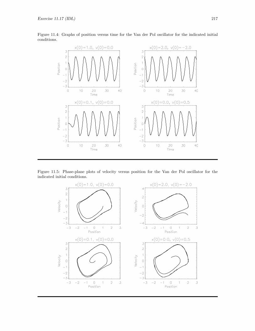
Exercise 11.17 (IDL) 217
Figure 11.4: Graphs of position versus time for the Van der Pol oscillator for the indicated initialconditions.
Figure 11.5: Phase-plane plots of velocity versus position for the Van der Pol oscillator for theindicated initial conditions.
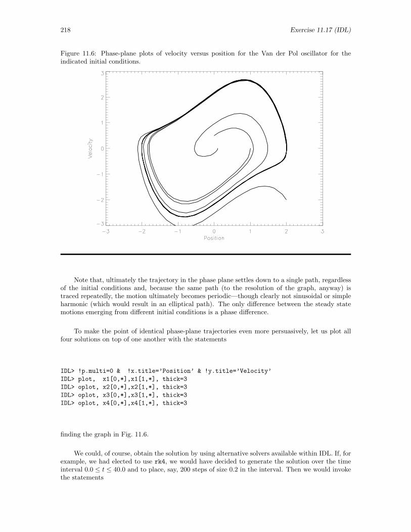
218 Exercise 11.17 (IDL)
Figure 11.6: Phase-plane plots of velocity versus position for the Van der Pol oscillator for theindicated initial conditions.
Note that, ultimately the trajectory in the phase plane settles down to a single path, regardlessof the initial conditions and, because the same path (to the resolution of the graph, anyway) istraced repeatedly, the motion ultimately becomes periodic—though clearly not sinusoidal or simpleharmonic (which would result in an elliptical path). The only difference between the steady statemotions emerging from different initial conditions is a phase difference.
To make the point of identical phase-plane trajectories even more persuasively, let us plot allfour solutions on top of one another with the statements
IDL> !p.multi=0 & !x.title=’Position’ & !y.title=’Velocity’
IDL> plot, x1[0,*],x1[1,*], thick=3
IDL> oplot, x2[0,*],x2[1,*], thick=3
IDL> oplot, x3[0,*],x3[1,*], thick=3
IDL> oplot, x4[0,*],x4[1,*], thick=3
finding the graph in Fig. 11.6.
We could, of course, obtain the solution by using alternative solvers available within IDL. If, forexample, we had elected to use rk4, we would have decided to generate the solution over the timeinterval 0.0 ≤ t ≤ 40.0 and to place, say, 200 steps of size 0.2 in the interval. Then we would invokethe statements
Exercise 11.17 (IDL) 219
IDL> t = findgen(201)/5.0
IDL> x = fltarr( 2, 201 )
IDL> x[0,0] = 1.0
IDL> dt = 0.2
IDL> for i=1, 200 do begin $
IDL> der = vandpol( t[i-1], x[*,i-1] ) & $
IDL> x[*,i] = rk4( x[*,i-1], der, t[i-1], $
IDL> dt, ’vandpol’ ) & $
IDL> endfor
IDL> x1 = x
Set times.Prepare two-column array for solution.Set initial conditions.Set time step.Loop once per point:Set current derivatives.Calculate solution dt later.
Save solution in new variable.
Repetition of this procedure will generate solutions for the other three initial conditions, whichsolutions can then be plotted by the same procedures as have already been illustrated to obtainbasically the same graphs. Note that, in this approach, we do not need to have four different vectorsfor the times because the solutions in each case are generated for the same times.
If, on the other hand, we had elected to use lsode, we would have decided to generate thesolution over the time interval 0.0 ≤ t ≤ 40.0 and to place, say, 200 steps of size 0.2 in the interval.Then we would invoke the statements
IDL> t = findgen(201)/5.0
IDL> x = fltarr( 2, 201 )
IDL> x[0,0] = 1.0
IDL> dt = 0.2
IDL> for i=1, 200 do begin $
IDL> tmp = x[*,i-1] & $
IDL> x[*,i] = lsode( tmp, t[i-1], dt, $
IDL> ’vandpol’ ) & $
IDL> endfor
IDL> x1 = x
Set times.Prepare two-column array for solution.Set initial conditions.Set time step.Loop once per point:Extract current values.Calculate solution dt later.
Save solution in new variable.
As with the rk4 solution, repetition of this procedure will generate solutions for the other threeinitial conditions, which solutions can then be plotted by the same procedures as have already beenillustrated to obtain basically the same graphs. Here again, we need not have four different vectorsfor the times because the solutions in each case are generated for the same times.
220 Exercise 11.18 (IDL)
11.18 Large Amplitude Pendulum (IDL)
Exercise: The angular position θ of a simple pendulum of length l satisfies the non-linearequation
d2θ
dt2+g
lsin θ = 0
where θ is measured in radians from the lowest point of the pendulum’s motion. Use numericalmethods to study the motion of this pendulum when it is released from rest at each of severalinitial displacements, say 20, 45, 90, 120, 150, 165, and 178. Look particularly at graphs ofθ versus t, dθ/dt versus t, and dθ/dt versus θ (the phase plot). Obtain also a graph of period versusamplitude (initial displacement). Write several paragraphs describing your set up of the problemand presenting evidence for your discoveries. Optional : Try starting the pendulum at the bottom(0 initial angle) with several initial angular velocities. How large can the angular velocity be beforethe pendulum begins to swing over the top? Suggestion: Begin by introducing the dimensionless
time t =√g/l t so that the equation becomes d2θ/dt
2+ sin θ = 0.
Solution: Starting with the equation
d2θ
dt2+g
lsin θ = 0
we begin by introducing the dimensionless time t =√g/l t, in terms of which the equation becomes
d2θ
dt2 + sin θ = 0
As a pair of first-order equations, we would alternatively have the two equations
dθ
dt= ω ;
dω
dt= − sin θ
(We have dropped the bars.) To address this equation numerically using IDL, we adopt the corre-spondences θ(t) 7→ x[0] and φ(t) 7→ x[1], and then we create the function pro-file
function sp0602, t, x
return, [x[1], -sin(x[0]) ]
end
and store it in the default directory with the name sp0602.pro. Then we invoke IDL with thecommand idl to the operating system and execute the following statements
ic = [ 15.0*!pi/180.0, 0.0 ]
ludiffeq_23, ’sp0602’, t, x, t0=0.0, tf = 10.0, init=ic
plot, t, x[0,*], thick=4
to set the initial conditions for release from rest at a displacement of 15, generate the solution overthe interval 0.0 < t < 10.0 at the default tolerance, and plot a graph of angular displacement as afunction of time for that interval. To check accuracy, we choose a smaller tolerance, regenerate thesolution, and overplot the results on the original graph with the statements
ludiffeq_23, ’sp0602’, t, x, t0=0.0, tf = 10.0, init=ic, tol = 0.0001
oplot, t, x[0,*], thick=4
Exercise 11.18 (IDL) 221
The two graphs lie essentially on top of one another throughout the entire range, from which weconclude that the solution generated with the first tolerance is, in fact, accurate to the resolutionof the graph (and may, in fact, be more accurate than that). (We elect not to display the graphsproduced by the statements in this paragraph.)
To produce a graph showing the behavior of this pendulum for several different amplitudes,we begin by setting a vector containing several different initial conditions (both in degrees and inradians) with the statements
phi0 = [20.0, 45.0, 90.0, 120.0, 150.0, 165.0, 178.0]
phi0rad = !pi*phi0/180.0
In trial runs, we discover (1) that we need to run the solution over the time interval 0.0 < t < 25.0 tocover the entire period of the motion at the largest amplitude and (2) that we must use a toleranceof 0.0001 rather than the default if we want to avoid the round off problems that cause the solutionat a tolerance of 0.001 to run over the top at the largest amplitude. Further, let’s set up so we canplot the angular displacement in degrees, which will range from −180 to 180 by establishing theaxes with the statement
plot, [0.0, 25.0], [-200.0, 200.0], /nodata, xtitle=’t’, $
ytitle=’!4h!3(t)’, ticklen=1.0
Then, we generate and plot each solution in turn within the loop
for i = 0, 6 do begin $
ic = [ phi0rad[i], 0.0 ] & $
ludiffeq_23, ’sp0602’, t, x, t0=0.0, tf = 25.0, init=ic, tol = 0.0001 & $
oplot, t, 180.0*x[0,*]/!pi, thick=4, linestyle=i & $
endfor
The resulting graph, the PostScript file for which was obtained by executing the statements
set_plot, ’ps’
device, filename = ’SP0602-fig1.ps’
plot, [0.0, 25.0], [-200.0, 200.0], /nodata, xtitle=’t’, $
ytitle=’!4h!3(t)’, ticklen=1.0
for i = 0, 6 do begin $
ic = [ phi0rad[i], 0.0 ] & $
ludiffeq_23, ’sp0602’, t, x, t0=0.0, tf = 25.0, init=ic, tol = 0.0001 & $
oplot, t, 180.0*x[0,*]/!pi, thick=4, linestyle=i & $
endfor
device, /close
set_plot, ’x’
is shown in Fig. 11.7. Note that the period gets longer as the amplitude increases and that thependulum dwells longer and longer near its highest point as the amplitude increases.
To plot angular velocity versus time, we need modify the above statements only slightly to be
plot, [0.0, 25.0], [-2.0, 2.0], /nodata, xtitle=’t’, $
ytitle=’!4x!3(t)’, ticklen=1.0
for i = 0, 6 do begin $
ic = [ phi0rad[i], 0.0 ] & $
ludiffeq_23, ’sp0602’, t, x, t0=0.0, tf = 25.0, init=ic, tol = 0.0001 & $
oplot, t, x[1,*], thick=4, linestyle=i & $
endfor
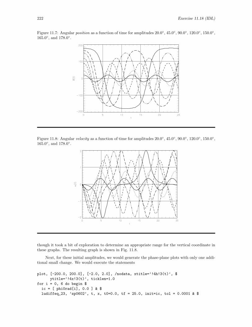
222 Exercise 11.18 (IDL)
Figure 11.7: Angular position as a function of time for amplitudes 20.0, 45.0, 90.0, 120.0, 150.0,165.0, and 178.0.
Figure 11.8: Angular velocity as a function of time for amplitudes 20.0, 45.0, 90.0, 120.0, 150.0,165.0, and 178.0.
though it took a bit of exploration to determine an appropriate range for the vertical coordinate inthese graphs. The resulting graph is shown in Fig. 11.8.
Next, for these initial amplitudes, we would generate the phase-plane plots with only one addi-tional small change. We would execute the statements
plot, [-200.0, 200.0], [-2.0, 2.0], /nodata, xtitle=’!4h!3(t)’, $
ytitle=’!4x!3(t)’, ticklen=1.0
for i = 0, 6 do begin $
ic = [ phi0rad[i], 0.0 ] & $
ludiffeq_23, ’sp0602’, t, x, t0=0.0, tf = 25.0, init=ic, tol = 0.0001 & $
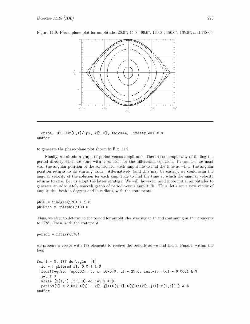
Exercise 11.18 (IDL) 223
Figure 11.9: Phase-plane plot for amplitudes 20.0, 45.0, 90.0, 120.0, 150.0, 165.0, and 178.0.
oplot, 180.0*x[0,*]/!pi, x[1,*], thick=4, linestyle=i & $
endfor
to generate the phase-plane plot shown in Fig. 11.9.
Finally, we obtain a graph of period versus amplitude. There is no simple way of finding theperiod directly when we start with a solution for the differential equation. In essence, we mustscan the angular position of the solution for each amplitude to find the time at which the angularposition returns to its starting value. Alternatively (and this may be easier), we could scan theangular velocity of the solution for each amplitude to find the time at which the angular velocityreturns to zero. Let us adopt the latter strategy. We will, however, need more initial amplitudes togenerate an adequately smooth graph of period versus amplitude. Thus, let’s set a new vector ofamplitudes, both in degrees and in radians, with the statements
phi0 = findgen(178) + 1.0
phi0rad = !pi*phi0/180.0
Thus, we elect to determine the period for amplitudes starting at 1 and continuing in 1 incrementsto 178. Then, with the statement
period = fltarr(178)
we prepare a vector with 178 elements to receive the periods as we find them. Finally, within theloop
for i = 0, 177 do begin $
ic = [ phi0rad[i], 0.0 ] & $
ludiffeq_23, ’sp0602’, t, x, t0=0.0, tf = 25.0, init=ic, tol = 0.0001 & $
j=5 & $
while (x[1,j] lt 0.0) do j=j+1 & $
period[i] = 2.0*( t[j] - x[1,j]*(t[j+1]-t[j])/(x[1,j+1]-x[1,j]) ) & $
endfor
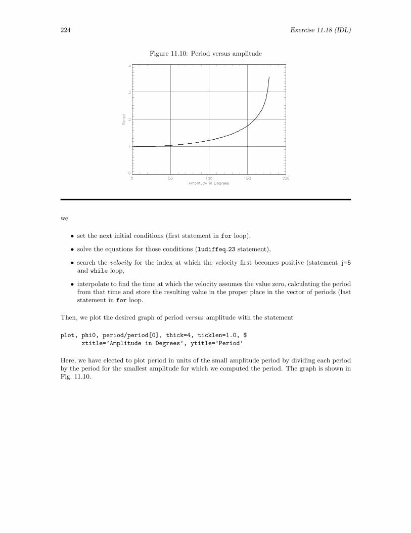
224 Exercise 11.18 (IDL)
Figure 11.10: Period versus amplitude
we
• set the next initial conditions (first statement in for loop),
• solve the equations for those conditions (ludiffeq 23 statement),
• search the velocity for the index at which the velocity first becomes positive (statement j=5
and while loop,
• interpolate to find the time at which the velocity assumes the value zero, calculating the periodfrom that time and store the resulting value in the proper place in the vector of periods (laststatement in for loop.
Then, we plot the desired graph of period versus amplitude with the statement
plot, phi0, period/period[0], thick=4, ticklen=1.0, $
xtitle=’Amplitude in Degrees’, ytitle=’Period’
Here, we have elected to plot period in units of the small amplitude period by dividing each periodby the period for the smallest amplitude for which we computed the period. The graph is shown inFig. 11.10.
Exercise 11.19 (IDL) 225
11.19 Planet in Non-Inverse Square Gravity (IDL)
Exercise: Suppose that the “gravitational” force were not inverse square but instead dependedon some other (negative) power of the radial coordinate. The dimensionless equations of motionthen would be
d2x
dt2 = − x
(x2 + y2)b;
d2y
dt2 = − y
(x2 + y2)b
Of course, the equations reduce to those for the inverse square force if we simply set b = 3/2. Forthe planetary problem, find conditions that will generate a distinctly elliptical orbit for an attractiveinverse square force (b = 1.5). Then explore the effect on that orbit of distorting the force bychanging the exponent in the denominator of the equations making b = 1.45, b = 1.55, or anythingelse you can think of, and write a paragraph or two describing the nature of the changes in somedetail. Make sure your solutions are generated to an adequate accuracy to support your conclusions.
Solution: The pro-file planet.pro deduced in Section 9.7.6 is designed to facilitate the explo-ration requested in this problem as well. With the correspondences vx 7→ x[0], x 7→ x[1], y 7→ x[2],and vy 7→ x[3], we there created the pro-file
FUNCTION planet, t, x
common params, b
temp = ( x[0]^2+x[2]^2 )^b
RETURN, [x[1], -x[0]/temp, x[3], -x[2]/temp ]
END
to return the derivatives of the four dependent variables involved in the set of four first-order ODEsdescribing the planetary problem. We have already determined that the initial conditions
x(0) = 4.0 ; vx(0) = 0.0 ; y(0) = 0.0 ; vy(0) = 0.3
lead to a distinctly elliptical orbit when b = 1.5 (inverse square force). Making sure to track farenough into the future for the planet to orbit its sun several times (and taking several preliminarytrials to find appropriate time intervals), we track the motion using different values of b with thestatements
IDL> ics = [ 4.0, 0.0, 0.0, 0.3 ]
IDL> common params, b
IDL> b = 1.50
IDL> ludiffeq_45, ’planet’, t1,x1, t0=0.0,tf=150, init=ics
IDL> b = 1.55
IDL> ludiffeq_45, ’planet’, t2,x2, t0=0.0,tf=150, init=ics
IDL> b = 1.45
IDL> ludiffeq_45, ’planet’, t3,x3, t0=0.0,tf=150, init=ics
IDL> b = 1.60
IDL> ludiffeq_45, ’planet’, t4,x4, t0=0.0,tf=150, init=ics
Then, plotting in order of increasing b and without struggling to arrange equal scales on the twoaxes, we plot the orbits with the statements
IDL> !p.multi=[0,2,2] & !x.range=[-4.0,4.0] & !y.range=[-4.0,4.0]
IDL> plot, x3[0,*],x3[2,*], thick=3, title=’b = 1.45’
IDL> plot, x1[0,*],x1[2,*], thick=3, title=’b = 1.50’
IDL> plot, x2[0,*],x2[2,*], thick=3, title=’b = 1.55’
IDL> plot, x4[0,*],x4[2,*], thick=3, title=’b = 1.60’
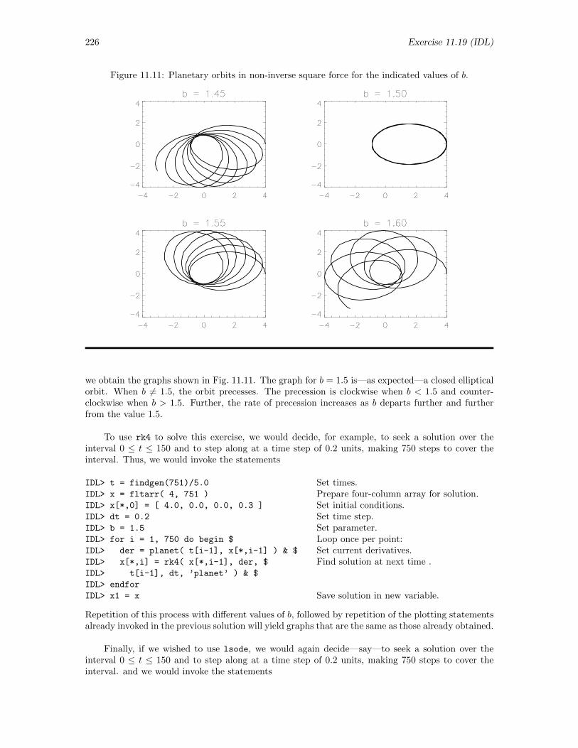
226 Exercise 11.19 (IDL)
Figure 11.11: Planetary orbits in non-inverse square force for the indicated values of b.
we obtain the graphs shown in Fig. 11.11. The graph for b = 1.5 is—as expected—a closed ellipticalorbit. When b 6= 1.5, the orbit precesses. The precession is clockwise when b < 1.5 and counter-clockwise when b > 1.5. Further, the rate of precession increases as b departs further and furtherfrom the value 1.5.
To use rk4 to solve this exercise, we would decide, for example, to seek a solution over theinterval 0 ≤ t ≤ 150 and to step along at a time step of 0.2 units, making 750 steps to cover theinterval. Thus, we would invoke the statements
IDL> t = findgen(751)/5.0
IDL> x = fltarr( 4, 751 )
IDL> x[*,0] = [ 4.0, 0.0, 0.0, 0.3 ]
IDL> dt = 0.2
IDL> b = 1.5
IDL> for i = 1, 750 do begin $
IDL> der = planet( t[i-1], x[*,i-1] ) & $
IDL> x[*,i] = rk4( x[*,i-1], der, $
IDL> t[i-1], dt, ’planet’ ) & $
IDL> endfor
IDL> x1 = x
Set times.Prepare four-column array for solution.Set initial conditions.Set time step.Set parameter.Loop once per point:Set current derivatives.Find solution at next time .
Save solution in new variable.
Repetition of this process with different values of b, followed by repetition of the plotting statementsalready invoked in the previous solution will yield graphs that are the same as those already obtained.
Finally, if we wished to use lsode, we would again decide—say—to seek a solution over theinterval 0 ≤ t ≤ 150 and to step along at a time step of 0.2 units, making 750 steps to cover theinterval. and we would invoke the statements
Exercise 11.19 (IDL) 227
IDL> t = findgen(751)/5.0
IDL> x = fltarr( 4, 751 )
IDL> x[*,0] = [ 4.0, 0.0, 0.0, 0.3 ]
IDL> dt = 0.2
IDL> b = 1.5
IDL> for i = 1, 750 do begin $
IDL> tmp = x[ *, i-1 ] & $
IDL> x[*,i] = lsode( tmp, t[i-1], $
IDL> dt, ’planet’ ) & $
IDL> endfor
IDL> x1 = x
Set times.Prepare four-column array for solution.Set initial conditions.Set time step.Set parameter.Loop once per point:Extract current values.Find solution at next time .
Save solution in new variable.
Again, repetition of this process with different values of b, followed by repetition of the plottingstatements already invoked in the previous solution will yield graphs that are the same as thosealready obtained.
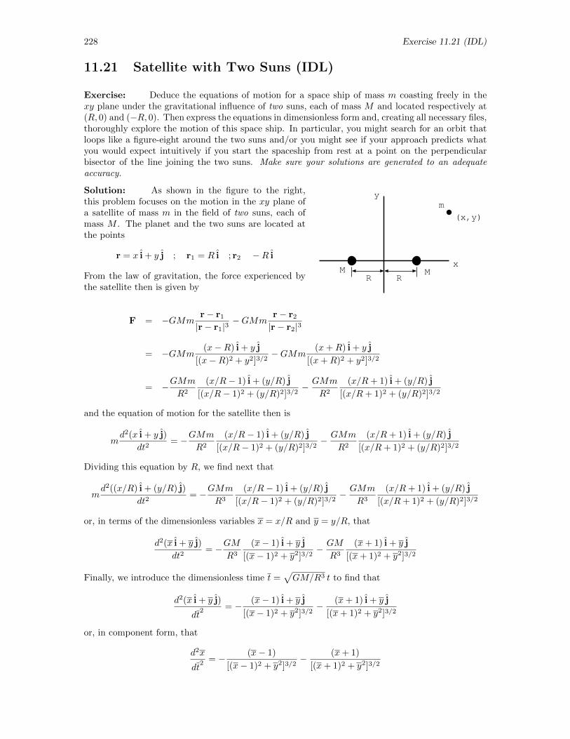
228 Exercise 11.21 (IDL)
11.21 Satellite with Two Suns (IDL)
Exercise: Deduce the equations of motion for a space ship of mass m coasting freely in thexy plane under the gravitational influence of two suns, each of mass M and located respectively at(R, 0) and (−R, 0). Then express the equations in dimensionless form and, creating all necessary files,thoroughly explore the motion of this space ship. In particular, you might search for an orbit thatloops like a figure-eight around the two suns and/or you might see if your approach predicts whatyou would expect intuitively if you start the spaceship from rest at a point on the perpendicularbisector of the line joining the two suns. Make sure your solutions are generated to an adequateaccuracy.
Solution: As shown in the figure to the right,this problem focuses on the motion in the xy plane ofa satellite of mass m in the field of two suns, each ofmass M . The planet and the two suns are located atthe points
r = x i + y j ; r1 = R i ; r2 −R i
From the law of gravitation, the force experienced bythe satellite then is given by
MM
m
x
y
R R
(x,y)
F = −GMmr− r1
|r− r1|3−GMm
r− r2
|r− r2|3
= −GMm(x−R) i + y j
[(x−R)2 + y2]3/2−GMm
(x+R) i + y j
[(x+R)2 + y2]3/2
= −GMm
R2
(x/R− 1) i + (y/R) j
[(x/R− 1)2 + (y/R)2]3/2− GMm
R2
(x/R+ 1) i + (y/R) j
[(x/R+ 1)2 + (y/R)2]3/2
and the equation of motion for the satellite then is
md2(x i + y j)
dt2= −GMm
R2
(x/R− 1) i + (y/R) j
[(x/R− 1)2 + (y/R)2]3/2− GMm
R2
(x/R+ 1) i + (y/R) j
[(x/R+ 1)2 + (y/R)2]3/2
Dividing this equation by R, we find next that
md2((x/R) i + (y/R) j)
dt2= −GMm
R3
(x/R− 1) i + (y/R) j
[(x/R− 1)2 + (y/R)2]3/2− GMm
R3
(x/R+ 1) i + (y/R) j
[(x/R+ 1)2 + (y/R)2]3/2
or, in terms of the dimensionless variables x = x/R and y = y/R, that
d2(x i + y j)
dt2= −GM
R3
(x− 1) i + y j
[(x− 1)2 + y2]3/2− GM
R3
(x+ 1) i + y j
[(x+ 1)2 + y2]3/2
Finally, we introduce the dimensionless time t =√GM/R3 t to find that
d2(x i + y j)
dt2 = − (x− 1) i + y j
[(x− 1)2 + y2]3/2− (x+ 1) i + y j
[(x+ 1)2 + y2]3/2
or, in component form, that
d2x
dt2 = − (x− 1)
[(x− 1)2 + y2]3/2− (x+ 1)
[(x+ 1)2 + y2]3/2
Exercise 11.21 ( IDL) 229
andd2y
dt2 = − y
[(x− 1)2 + y2]3/2− y
[(x+ 1)2 + y2]3/2
Then, with the correspondences x 7→ pos[0], dx/dt 7→ pos[1], y 7→ pos[2], and dx/dt 7→ pos[3], wewould construct the pro-file
FUNCTION twosuns, t, pos
tmp1 = 1.0 / ( (pos[0] - 1.0)^2 + pos[2]^2 )^1.5
tmp2 = 1.0 / ( (pos[0] + 1.0)^2 + pos[2]^2 )^1.5
xacc = -(pos[0] - 1.0)*tmp1 - (pos[0] + 1.0)*tmp2
yacc = -pos[2] * (tmp1 + tmp2)
RETURN, [ pos[1], xacc, pos[3], yacc ]
END
As a first test of the above analysis and the pro-file we have created, let us ask about the motionwhen the satellite is released from rest at a point on the y axis. The statements
IDL> ics = [0.0, 0.0, 2.0, 0.0 ]
IDL> ludiffeq_23, ’twosuns’, t1, x1, t0=0.0,tf=50.0, init=ics
IDL> plot, x1[0,*], x1[2,*], xrange=[-0.4,0.4]
IDL> plot, t1, x1[0,*]
IDL> plot, t1, x1[2,*], yrange=[-0.4,0.4]
produce three graphs (not shown) in which (1) the trajectory of the satellite is confined to the y axis,(2) the y coordinate oscillates through several cycles, staying in the interval −2.0 ≤ y ≤ 2.0, and(3) the x coordinate stays fixed at x = 0.0. All of this is as expected and provides some evidence ofthe adequacy of the specified default tolerance. [In the first and third cases, explicit specification ofthe range on one of the axes is necessary. Otherwise, IDL will choose to start the axis at the value0.0, and the graph will lie right on the axis (and thus be invisible).]
Next, again as a test, we suppose that the satellite is started off quite some distance from thetwo suns on the x axis and given a velocity perpendicular to that axis (i.e., a y velocity only). Aftersome exploration with the y velocity, we invoke the statements
IDL> ics = [20.0, 0.0, 0.0, 0.3 ]
IDL> ludiffeq_23, ’twosuns’, t1, x1, t0=0.0,tf=400.0, init=ics, tol=1.0e-6
IDL> plot, x1[0,*], x1[2,*]
which generates a graph (again, not shown) of a closed orbit around both suns. This result, too, isexpected, since from a distance 10 times the separation of the two suns, the two suns look almostlike a single sun of twice the mass, and the orbit should be close to the ellipse we would expect ifthere were only one sun. This outcome provides further justification of the adequacy of our approachand choice of tolerances. (Actually, in this latter case, the tolerance was made more stringent notso much as to produce a closed orbit—the default tolerance did that tolerably well—but to producea smoother curve, since the default tolerance stepped along the path so quickly that the resultinggraph was a bit jagged.)
Finally, let’s move the satellite in a bit closer and explore a few trajectories with different initialconditions:5,6 (a) Start on the y axis with an initial x velocity:
5Some exploration was needed before the initial conditions actually presented were identified.6If, as you explore this problem, the message ‘Beware of singularity’ appears, you should simply conclude that
the adaptive algorithm failed to converge at some point after executing the maximum number of iterations, and thesolution was terminated. The satellite probably collided with one of the suns, and a plot of the data that IDL doesreturn will probably reveal as much.
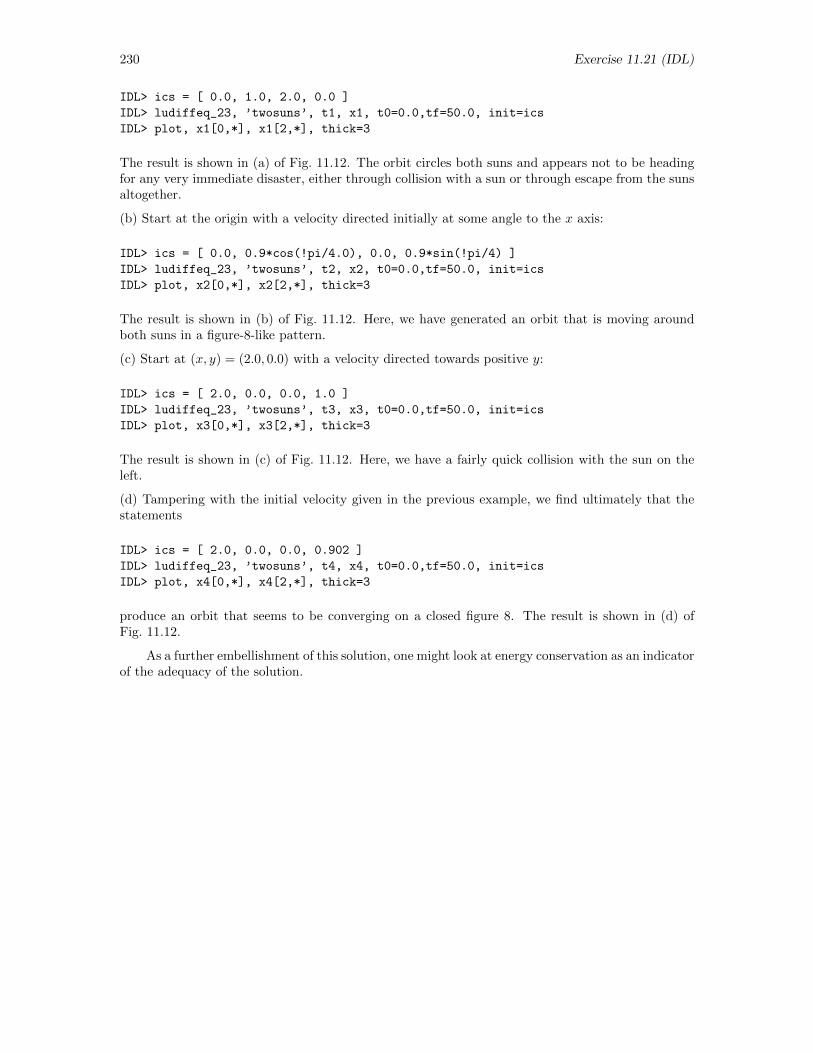
230 Exercise 11.21 (IDL)
IDL> ics = [ 0.0, 1.0, 2.0, 0.0 ]
IDL> ludiffeq_23, ’twosuns’, t1, x1, t0=0.0,tf=50.0, init=ics
IDL> plot, x1[0,*], x1[2,*], thick=3
The result is shown in (a) of Fig. 11.12. The orbit circles both suns and appears not to be headingfor any very immediate disaster, either through collision with a sun or through escape from the sunsaltogether.
(b) Start at the origin with a velocity directed initially at some angle to the x axis:
IDL> ics = [ 0.0, 0.9*cos(!pi/4.0), 0.0, 0.9*sin(!pi/4) ]
IDL> ludiffeq_23, ’twosuns’, t2, x2, t0=0.0,tf=50.0, init=ics
IDL> plot, x2[0,*], x2[2,*], thick=3
The result is shown in (b) of Fig. 11.12. Here, we have generated an orbit that is moving aroundboth suns in a figure-8-like pattern.
(c) Start at (x, y) = (2.0, 0.0) with a velocity directed towards positive y:
IDL> ics = [ 2.0, 0.0, 0.0, 1.0 ]
IDL> ludiffeq_23, ’twosuns’, t3, x3, t0=0.0,tf=50.0, init=ics
IDL> plot, x3[0,*], x3[2,*], thick=3
The result is shown in (c) of Fig. 11.12. Here, we have a fairly quick collision with the sun on theleft.
(d) Tampering with the initial velocity given in the previous example, we find ultimately that thestatements
IDL> ics = [ 2.0, 0.0, 0.0, 0.902 ]
IDL> ludiffeq_23, ’twosuns’, t4, x4, t0=0.0,tf=50.0, init=ics
IDL> plot, x4[0,*], x4[2,*], thick=3
produce an orbit that seems to be converging on a closed figure 8. The result is shown in (d) ofFig. 11.12.
As a further embellishment of this solution, one might look at energy conservation as an indicatorof the adequacy of the solution.
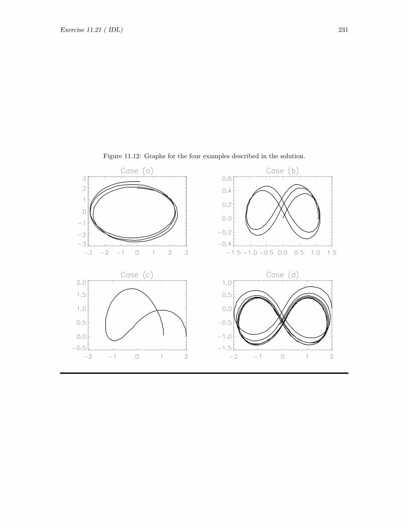
Exercise 11.21 ( IDL) 231
Figure 11.12: Graphs for the four examples described in the solution.
232 Exercise 11.22 (IDL)
11.22 Charge in Crossed Fields (IDL)
Exercise: Suppose a particle of charge q and mass m is injected into a region of space containingconstant, crossed electric and magnetic fields E = Exi and B = Bzk. In vector form, the equationof motion for this particle is
md2r
dt2= qE + q
dr
dt×B
Verify the equations of motion
md2x
dt2= qEx + qBz
dy
dt; m
d2y
dt2= −qBz
dx
dt; m
d2z
dt2= 0
for the specific fields of this exercise, express them in dimensionless form (note that ω = qBz/m isa frequency and Ex/Bz is a velocity), and thoroughly explore the behavior of the particle in thissituation. Try to understand the motion intuitively. Hint : You should find that, in terms of anarbitrarily selected unit of length `, the equations involve a single parameter qEx/(mω
2`), whichcan alternatively be written as (Ex/Bz)/(ω`) — the ratio of the velocity Ex/Bz determined by thefields to the characteristic velocity implied by your choice of a length unit and the frequency ω.Note that this exercise actually has more than one parameter, since the initial components of thevelocity—probably expressed in units of ω`—also influence the solution.
Solution: The first part of this exercise is to verify the second set of equations from the firstset. We begin by substituting components for all the vectors in the basic equation, finding that
md2(x i + y j + z k)
dt2= qEx i + q
d(x i + y j + z k)
dt×Bz k
= qEx i + qBzd(−x j + y i)
dt
The desired equations are the x, y, and z components of this vector equation.
The second part of the exercise asks us to cast these individual equations in dimensionless form.Dividing all three equations by m, we obtain
d2x
dt2=qExm
+ ωdy
dt;
d2y
dt2= −ωdx
dt;
d2z
dt2= 0
Now, setting x = x/`, y = y/`, z = z/`, and t = ωt, we find that
d2x
dt2=
qExmω2`
+dy
dt;
d2y
dt2= −dx
dt;
d2z
dt2= 0
Hereafter, we drop the overbars and use the symbol w to stand for qEx/mω2`.
At this point, we recognize that the motion in the z-direction is motion with zero acceleration,which implies constant velocity. That motion is independent of the projection of the motion into thexy-plane. Consequently, we can focus on the x and y motion. To set up the function that will definethe x and y equations for IDL’s procedure lsode, we begin by establishing the correspondences
x→ n[0], y → n[1],dx
dt→ n[2],
dy
dt→ n[3]
in terms of which the equations become
dn[0]
dt= n[2],
dn[1]
dt= n[3],
dn[2]
dt= w + n[3],
dn[3]
dt= −n[2]
and the function defining these equations for lsode then is
Exercise 11.22 (IDL) 233
FUNCTION charge, t, n
;+
; charge.pro takes as its second argument a
; four-component vector whose components are
; x, y, vx, vy and returns the first derivatives
; of these quantities n = [vx, vy, w+vy, -vx]
;-
common params, w
return, [n[2],n[3],w+n[3],-n[2]]
END
Here, we have used a common storage to communicate the parameter w from command level throughludiffeq 23 to the function charge.
Once this function has been defined in IDL, we can find and plot the solution for several valuesof w when the particle is started off at the origin at rest with the coding
common params, w
ic = [0.0,0.0,0.0,0.0]
!p.multi = [0,2,2]
w = 0.2
ludiffeq_23, ’charge’, t, n02, t0=0.0, tf=20.0, init = ic
plot, n02[0,*], n02[1,*], thick = 3.0, title = ’w = ’ + $
string(w,format=’(f4.1)’), ytitle = ’y(t)’, xtitle = ’x(t)’
w = 0.5
ludiffeq_23, ’charge’, t, n05, t0=0.0, tf=20.0, init = ic
plot, n05[0,*], n05[1,*], thick = 3.0, title = ’w = ’ + $
string(w,format=’(f4.1)’), ytitle = ’y(t)’, xtitle = ’x(t)’
w = 1.0
ludiffeq_23, ’charge’, t, n10, t0=0.0, tf=20.0, init = ic
plot, n10[0,*], n10[1,*], thick = 3.0, title = ’w = ’ + $
string(w,format=’(f4.1)’), ytitle = ’y(t)’, xtitle = ’x(t)’
w = 1.5
ludiffeq_23, ’charge’, t, n15, t0=0.0, tf=20.0, init = ic
plot, n15[0,*], n15[1,*], thick = 3.0, title = ’w = ’ + $
string(w,format=’(f4.1)’), ytitle = ’y(t)’, xtitle = ’x(t)’
The four graphs generated by this code are shown in Fig. 11.13. The general trajectory has the sameform for all values of w. Only the scale along both axes changes. Because of the electric field in thei direction, this particle is initially accelerated in that direction. Once the particle starts moving,however, the magnetic field exerts an additional force in the direction i × k = − j, so the particleis nudged in the negative y direction. Overall, the particle oscillates in the x direction but drifts inthe minus-y direction.
Graphs of x, y, vx, and vy as functions of t for w = 0.5 can be produced with the statements
!p.multi = [0,2,2]
plot, t, n05[0,*], thick = 3.0, title = ’x vs.t.for w = ’ + $
string(w,format=’(f4.1)’), ytitle = ’x(t)’, xtitle = ’t’
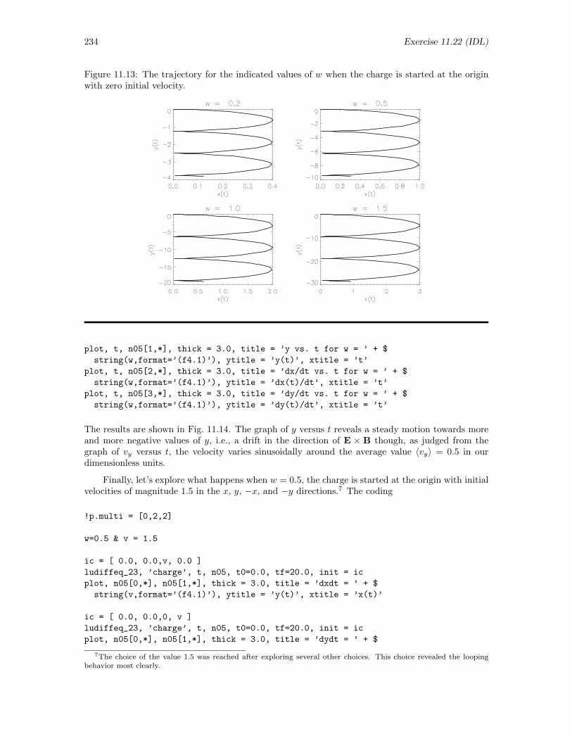
234 Exercise 11.22 (IDL)
Figure 11.13: The trajectory for the indicated values of w when the charge is started at the originwith zero initial velocity.
plot, t, n05[1,*], thick = 3.0, title = ’y vs. t for w = ’ + $
string(w,format=’(f4.1)’), ytitle = ’y(t)’, xtitle = ’t’
plot, t, n05[2,*], thick = 3.0, title = ’dx/dt vs. t for w = ’ + $
string(w,format=’(f4.1)’), ytitle = ’dx(t)/dt’, xtitle = ’t’
plot, t, n05[3,*], thick = 3.0, title = ’dy/dt vs. t for w = ’ + $
string(w,format=’(f4.1)’), ytitle = ’dy(t)/dt’, xtitle = ’t’
The results are shown in Fig. 11.14. The graph of y versus t reveals a steady motion towards moreand more negative values of y, i.e., a drift in the direction of E × B though, as judged from thegraph of vy versus t, the velocity varies sinusoidally around the average value 〈vy〉 = 0.5 in ourdimensionless units.
Finally, let’s explore what happens when w = 0.5, the charge is started at the origin with initialvelocities of magnitude 1.5 in the x, y, −x, and −y directions.7 The coding
!p.multi = [0,2,2]
w=0.5 & v = 1.5
ic = [ 0.0, 0.0,v, 0.0 ]
ludiffeq_23, ’charge’, t, n05, t0=0.0, tf=20.0, init = ic
plot, n05[0,*], n05[1,*], thick = 3.0, title = ’dxdt = ’ + $
string(v,format=’(f4.1)’), ytitle = ’y(t)’, xtitle = ’x(t)’
ic = [ 0.0, 0.0,0, v ]
ludiffeq_23, ’charge’, t, n05, t0=0.0, tf=20.0, init = ic
plot, n05[0,*], n05[1,*], thick = 3.0, title = ’dydt = ’ + $
7The choice of the value 1.5 was reached after exploring several other choices. This choice revealed the loopingbehavior most clearly.
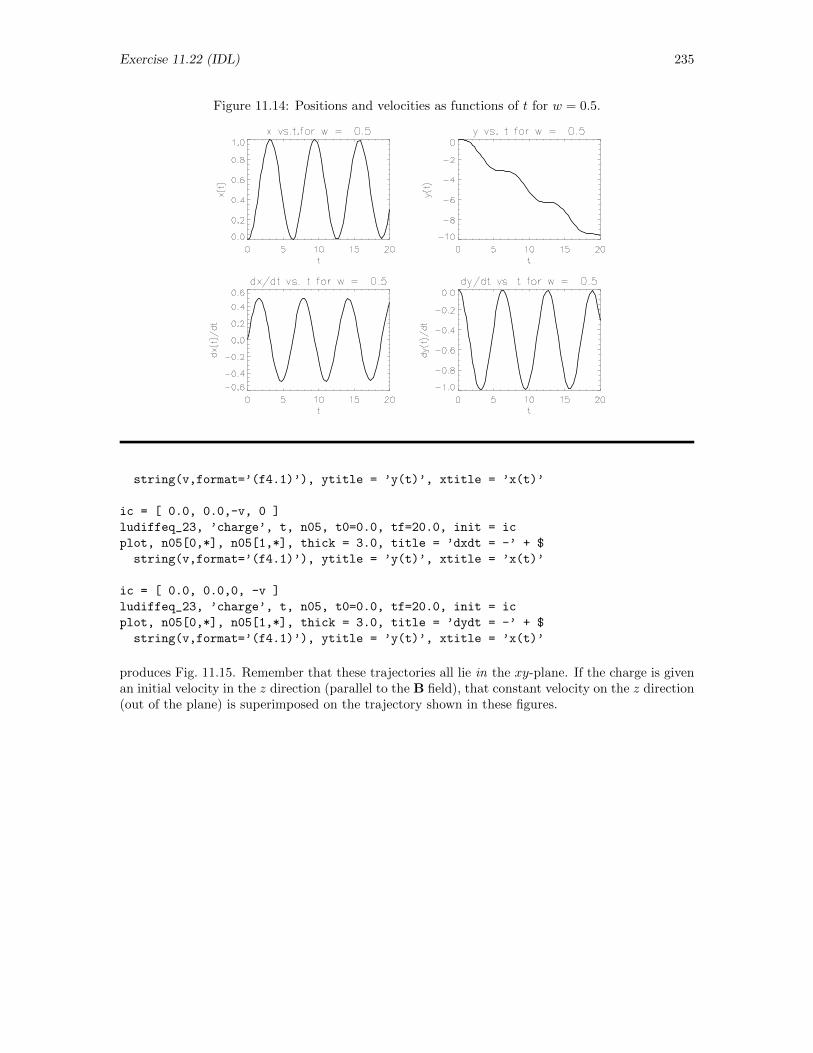
Exercise 11.22 (IDL) 235
Figure 11.14: Positions and velocities as functions of t for w = 0.5.
string(v,format=’(f4.1)’), ytitle = ’y(t)’, xtitle = ’x(t)’
ic = [ 0.0, 0.0,-v, 0 ]
ludiffeq_23, ’charge’, t, n05, t0=0.0, tf=20.0, init = ic
plot, n05[0,*], n05[1,*], thick = 3.0, title = ’dxdt = -’ + $
string(v,format=’(f4.1)’), ytitle = ’y(t)’, xtitle = ’x(t)’
ic = [ 0.0, 0.0,0, -v ]
ludiffeq_23, ’charge’, t, n05, t0=0.0, tf=20.0, init = ic
plot, n05[0,*], n05[1,*], thick = 3.0, title = ’dydt = -’ + $
string(v,format=’(f4.1)’), ytitle = ’y(t)’, xtitle = ’x(t)’
produces Fig. 11.15. Remember that these trajectories all lie in the xy-plane. If the charge is givenan initial velocity in the z direction (parallel to the B field), that constant velocity on the z direction(out of the plane) is superimposed on the trajectory shown in these figures.
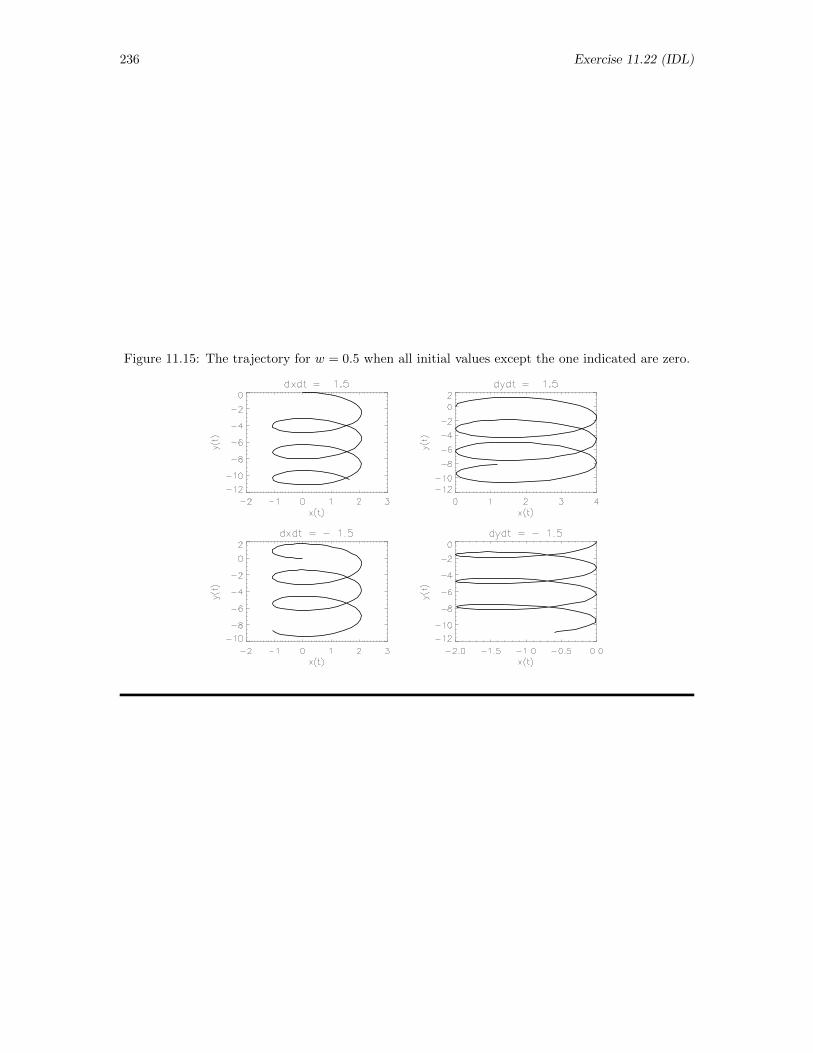
236 Exercise 11.22 (IDL)
Figure 11.15: The trajectory for w = 0.5 when all initial values except the one indicated are zero.
Exercise 11.24 (IDL) 237
11.24 The Lorenz Attractor (IDL)
Exercise: An important system in the early study of chaos is described by the Lorenz equations
dx
dt= a(y − x)
dy
dt= −xz + bx− y
dz
dt= xy − cz
Create an appropriate file defining these equations and then thoroughly explore the behavior of thissystem. Graphs of y versus x, z versus x, and z versus y when a = 10.0, b = 28.0 and c = 8.0/3.0under the initial conditions x0 = 1.0, y0 = 0.0, and z0 = 0.0 are particularly interesting. Whilegraphs of y versus x, z versus x, and z versus y are interesting, the true beauty of the trajectory isbest seen using a three-dimensional space curve. Be sure to examine the path from several differentvantage points in the space around the path, an objective most easily accomplished if the display ofthe path allows rotation of the path on the screen.
Solution: For the Lorenz system with three parameters a, b, and c, we declare the correspon-dences x 7→ var[0], y 7→ var[1], and z 7→ var[2]. Then, we create the pro-file
FUNCTION lorenz, t, var
common params, a, b, c
dxdt = a*(var[1]-var[0])
dydt = -var[0]*var[2] + b*var[0]
dzdt = var[0]*var[1] - c*var[2]
RETURN, [ dxdt, dydt, dzdt ]
END
which returns the derivatives of the dependent variables. We elect to use lsode. Then, to find asolution over the time interval from 0.0 ≤ t ≤ 50.0 (which is a guess as to an appropriate interval)with 2000 steps8 in that interval and the parameters given in the exercise, we use the statements
IDL> t = findgen(2001)/40.0
IDL> sln = fltarr( 3, 2001 )
IDL> sln[*,0] = [ 5.0, 0.0, 0.0 ]
IDL> dt = 0.025
IDL> common params, a, b, c
IDL> a = 10.0 & b = 28.0 & c = 8.0/3.0
IDL> for i = 1, 2000 do begin $
IDL> tmp = sln[*,i-1] & $
IDL> sln[*,i] = lsode( tmp, t[i-1], $
IDL> dt, ’lorenz’ ) & $
IDL> endfor
IDL> sln1 = sln
Set times.Prepare three-column array for solution.Set initial values.Set time step.Define common area for parameters.Set parameters.Loop once per point:Extract solution at current time.Generate solution at next time.
Save solution.
With this solution now in hand, we can generate several graphs. First we look at the behaviorof each state variable as a function of time with the statements
IDL> !p.multi=[0,2,2]
IDL> plot, t, sln1[0,*], title=’X1 versus T’
IDL> plot, t, sln1[1,*], title=’X2 versus T’
IDL> plot, t, sln1[2,*], title=’X3 versus T’
8The initial try used 200 steps, but that value led to major jaggedness in some of the graphs.
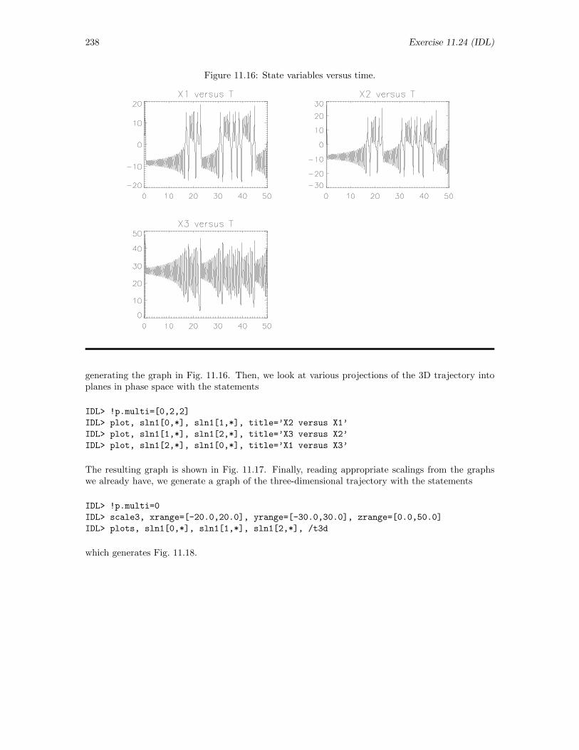
238 Exercise 11.24 (IDL)
Figure 11.16: State variables versus time.
generating the graph in Fig. 11.16. Then, we look at various projections of the 3D trajectory intoplanes in phase space with the statements
IDL> !p.multi=[0,2,2]
IDL> plot, sln1[0,*], sln1[1,*], title=’X2 versus X1’
IDL> plot, sln1[1,*], sln1[2,*], title=’X3 versus X2’
IDL> plot, sln1[2,*], sln1[0,*], title=’X1 versus X3’
The resulting graph is shown in Fig. 11.17. Finally, reading appropriate scalings from the graphswe already have, we generate a graph of the three-dimensional trajectory with the statements
IDL> !p.multi=0
IDL> scale3, xrange=[-20.0,20.0], yrange=[-30.0,30.0], zrange=[0.0,50.0]
IDL> plots, sln1[0,*], sln1[1,*], sln1[2,*], /t3d
which generates Fig. 11.18.
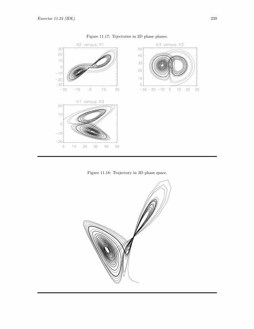
Exercise 11.24 (IDL) 239
Figure 11.17: Trjectories in 2D phase planes.
Figure 11.18: Trajectory in 3D phase space.
240 Exercise 11.27 (IDL)
11.27 Dynamics of a Chemical Reaction (IDL)
Exercise: The dynamics of the chemical reaction
A + B C + D
is governed by the equations
dA
dt= −kfAB + krCD
dB
dt= −kfAB + krCD
dC
dt= kfAB − krCD
dD
dt= kfAB − krCD
where A(t), B(t), C(t), and D(t) are the concentrations of each molecule in the reaction vessel, andkf and kr are the forward and reverse rate constants, respectively. Suppose that the reaction isstarted with A(0) = A0, B(0) = B0, and C(0) = D(0) = 0. Cast the equations in dimensionlessform, using A0 as the unit of concentration and kfA0t as the dimensionless time. Then explorethe behavior of the system as a function of the initial concentration of B, measured in units ofA0 and the reverse rate constant, measured in units of kf . Look particularly at the dependence ofthe ultimate equilibrium on these parameters. Make sure your results are generated to adequateaccuracy.
Solution: To put the above equations into dimensionless form, we first need to realize thatthis system of equations is not linear. A,B,C, and D are all in units of concentration, meaning thatwe have concentration-squared on the right side and concentration-over-time on the left. Because ofthis, we must introduce units of inverse concentration for the constants kf and kr. Since the unitsare consistent on both sides now, we can substitute AB = (AB)/A2
0, CD = (CD)/A20 and absorb
the extra A0 term into the time variable, t = t(kfA0). Dividing through by kf and dropping thebars then yields the dimensionless equations
dA
dt= −AB +
krkfCD
dB
dt= −AB +
krkfCD
dC
dt= AB − kr
kfCD
dD
dt= AB − kr
kfCD
To write the function defining these equations for OCTAVE’s routine lsode, we establish theassociations
A =⇒ n[0] ; B =⇒ n[1] ; C =⇒ n[2] ; D =⇒ n[3]
and introduce k to stand for kr/kf . In these terms, the equations become
dn[0]
dt= −n[0] ∗ n[1] + k ∗ n[2] ∗ n[3]
dn[1]
dt= −n[0] ∗ n[1] + k ∗ n[2] ∗ n[3]
dn[2]
dt= n[0] ∗ n[1]− k ∗ n[2] ∗ n[3]
dn[3]
dt= n[0] ∗ n[1]− k ∗ n[2] ∗ n[3]
These equations can then be solved and plotted in OCTAVE in the standard way of creating graphsof ODEs. With the parameter k being communicated from command level through ludiffeq 23 tothe function in common storage, the procedure file chemreac.pro defined with the statements
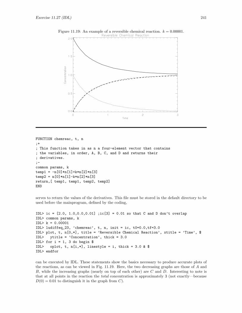
Exercise 11.27 (IDL) 241
Figure 11.19: An example of a reversible chemical reaction. k = 0.00001.
FUNCTION chemreac, t, n
;+
; This function takes in as n a four-element vector that contains
; the variables, in order, A, B, C, and D and returns their
; derivatives.
;-
common params, k
temp1 = -n[0]*n[1]+k*n[2]*n[3]
temp2 = n[0]*n[1]-k*n[2]*n[3]
return,[ temp1, temp1, temp2, temp2]
END
serves to return the values of the derivatives. This file must be stored in the default directory to beused before the mainprogram, defined by the coding,
IDL> ic = [2.0, 1.0,0.0,0.01] ;ic[3] = 0.01 so that C and D don’t overlap
IDL> common params, k
IDL> k = 0.00001
IDL> ludiffeq_23, ’chemreac’, t, n, init = ic, t0=0.0,tf=3.0
IDL> plot, t, n[0,*], title = ’Reversible Chemical Reaction’, xtitle = ’Time’, $
IDL> ytitle = ’Concentration’, thick = 3.0
IDL> for i = 1, 3 do begin $
IDL> oplot, t, n[i,*], linestyle = i, thick = 3.0 & $
IDL> endfor
can be executed by IDL. These statements show the basics necessary to produce accurate plots ofthe reactions, as can be viewed in Fig. 11.19. Here, the two decreasing graphs are those of A andB, while the increasing graphs (nearly on top of each other) are C and D. Interesting to note isthat at all points in the reaction the total concentration is approximately 3 (not exactly—becauseD(0) = 0.01 to distinguish it in the graph from C).
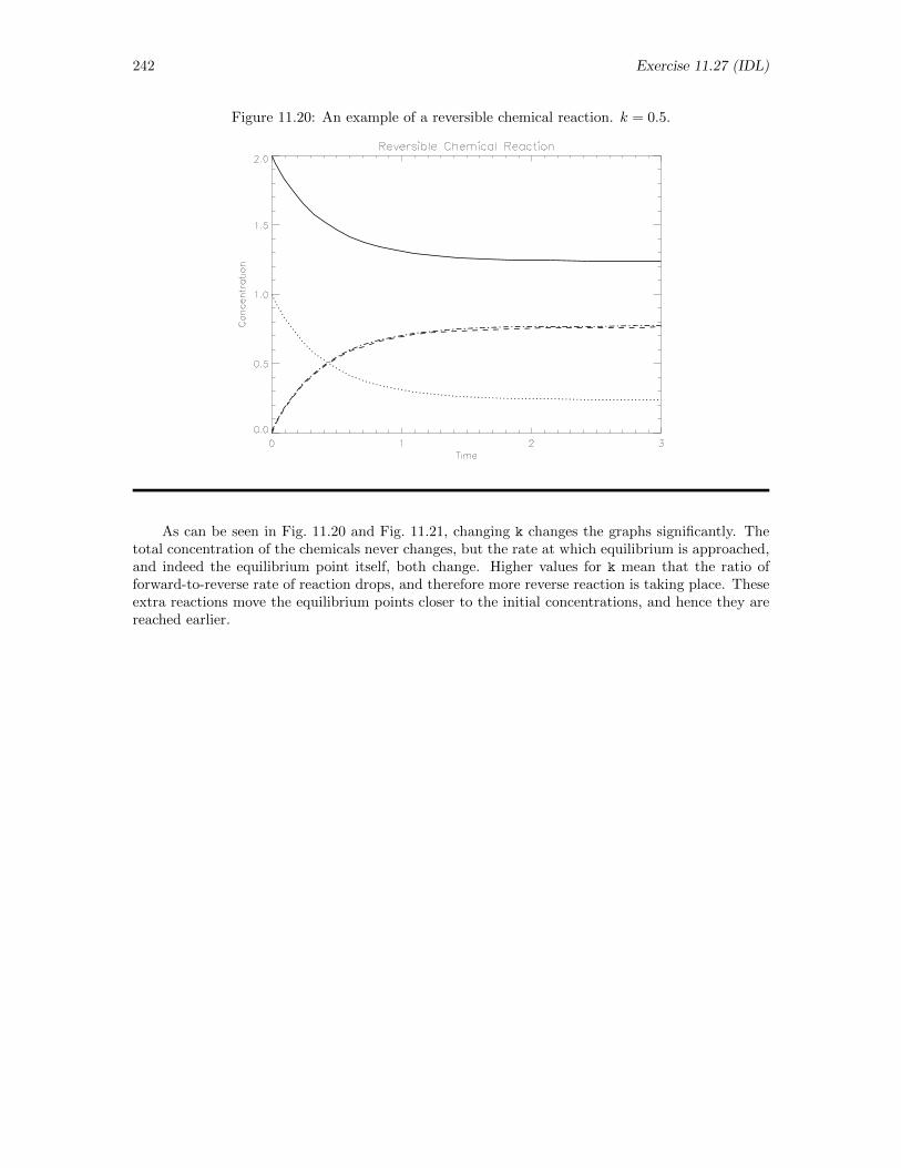
242 Exercise 11.27 (IDL)
Figure 11.20: An example of a reversible chemical reaction. k = 0.5.
As can be seen in Fig. 11.20 and Fig. 11.21, changing k changes the graphs significantly. Thetotal concentration of the chemicals never changes, but the rate at which equilibrium is approached,and indeed the equilibrium point itself, both change. Higher values for k mean that the ratio offorward-to-reverse rate of reaction drops, and therefore more reverse reaction is taking place. Theseextra reactions move the equilibrium points closer to the initial concentrations, and hence they arereached earlier.
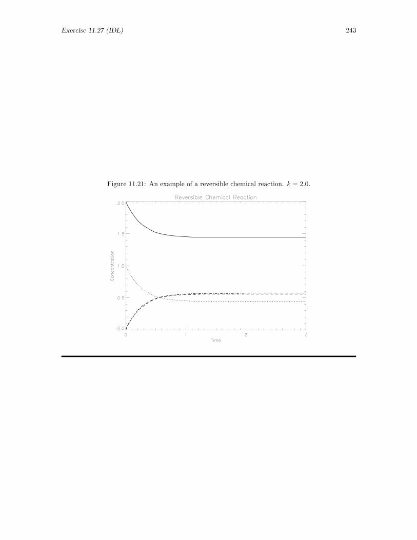
Exercise 11.27 (IDL) 243
Figure 11.21: An example of a reversible chemical reaction. k = 2.0.
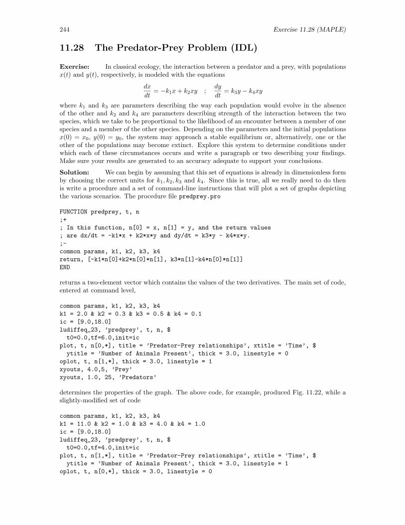
244 Exercise 11.28 (MAPLE)
11.28 The Predator-Prey Problem (IDL)
Exercise: In classical ecology, the interaction between a predator and a prey, with populationsx(t) and y(t), respectively, is modeled with the equations
dx
dt= −k1x+ k2xy ;
dy
dt= k3y − k4xy
where k1 and k3 are parameters describing the way each population would evolve in the absenceof the other and k2 and k4 are parameters describing strength of the interaction between the twospecies, which we take to be proportional to the likelihood of an encounter between a member of onespecies and a member of the other species. Depending on the parameters and the initial populationsx(0) = x0, y(0) = y0, the system may approach a stable equilibrium or, alternatively, one or theother of the populations may become extinct. Explore this system to determine conditions underwhich each of these circumstances occurs and write a paragraph or two describing your findings.Make sure your results are generated to an accuracy adequate to support your conclusions.
Solution: We can begin by assuming that this set of equations is already in dimensionless formby choosing the correct units for k1, k2, k3 and k4. Since this is true, all we really need to do thenis write a procedure and a set of command-line instructions that will plot a set of graphs depictingthe various scenarios. The procedure file predprey.pro
FUNCTION predprey, t, n
;+
; In this function, n[0] = x, n[1] = y, and the return values
; are dx/dt = -k1*x + k2*x*y and dy/dt = k3*y - k4*x*y.
;-
common params, k1, k2, k3, k4
return, [-k1*n[0]+k2*n[0]*n[1], k3*n[1]-k4*n[0]*n[1]]
END
returns a two-element vector which contains the values of the two derivatives. The main set of code,entered at command level,
common params, k1, k2, k3, k4
k1 = 2.0 & k2 = 0.3 & k3 = 0.5 & k4 = 0.1
ic = [9.0,18.0]
ludiffeq_23, ’predprey’, t, n, $
t0=0.0,tf=6.0,init=ic
plot, t, n[0,*], title = ’Predator-Prey relationships’, xtitle = ’Time’, $
ytitle = ’Number of Animals Present’, thick = 3.0, linestyle = 0
oplot, t, n[1,*], thick = 3.0, linestyle = 1
xyouts, 4.0,5, ’Prey’
xyouts, 1.0, 25, ’Predators’
determines the properties of the graph. The above code, for example, produced Fig. 11.22, while aslightly-modified set of code
common params, k1, k2, k3, k4
k1 = 11.0 & k2 = 1.0 & k3 = 4.0 & k4 = 1.0
ic = [9.0,18.0]
ludiffeq_23, ’predprey’, t, n, $
t0=0.0,tf=4.0,init=ic
plot, t, n[1,*], title = ’Predator-Prey relationships’, xtitle = ’Time’, $
ytitle = ’Number of Animals Present’, thick = 3.0, linestyle = 1
oplot, t, n[0,*], thick = 3.0, linestyle = 0
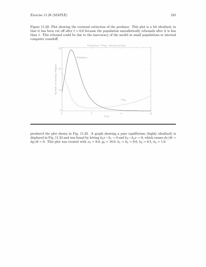
Exercise 11.28 (MAPLE) 245
Figure 11.22: Plot showing the eventual extinction of the predator. This plot is a bit idealized, inthat it has been cut off after t = 6.0 because the population unrealistically rebounds after it is lessthan 1. This rebound could be due to the inaccuracy of the model at small populations or internalcomputer roundoff.
produced the plot shown in Fig. 11.23. A graph showing a pure equilibrium (highly idealized) isdisplayed in Fig. 11.24 and was found by letting k2x−k1 = 0 and k3−k4x = 0, which causes dx/dt =dy/dt = 0. This plot was created with x0 = 9.0, y0 = 18.0, k1 = k3 = 9.0, k2 = 0.5, k4 = 1.0.
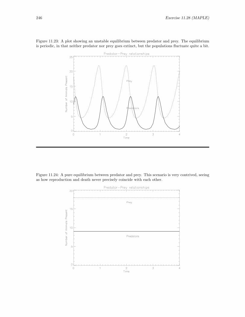
246 Exercise 11.28 (MAPLE)
Figure 11.23: A plot showing an unstable equilibrium between predator and prey. The equilibriumis periodic, in that neither predator nor prey goes extinct, but the populations fluctuate quite a bit.
Figure 11.24: A pure equilibrium between predator and prey. This scenario is very contrived, seeingas how reproduction and death never precisely coincide with each other.
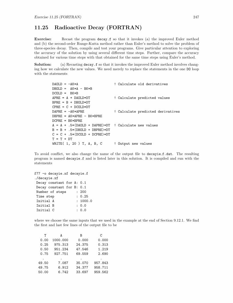
Exercise 11.25 (FORTRAN) 247
11.25 Radioactive Decay (FORTRAN)
Exercise: Recast the program decay.f so that it invokes (a) the improved Euler methodand (b) the second-order Runge-Kutta method rather than Euler’s method to solve the problem ofthree-species decay. Then, compile and test your programs. Give particular attention to exploringthe accuracy of the solution by using several different time steps. Further, compare the accuracyobtained for various time steps with that obtained for the same time steps using Euler’s method.
Solution: (a) Recasting decay.f so that it invokes the improved Euler method involves chang-ing how we calculate the new values. We need merely to replace the statements in the one DO loopwith the statements
DAOLD = -AK*A ! Calculate old derivatives
DBOLD = AK*A - BK*B
DCOLD = BK*B
APRE = A + DAOLD*DT ! Calculate predicted values
BPRE = B + DBOLD*DT
CPRE = C + DCOLD*DT
DAPRE = -AK*APRE ! Calculate predicted derivatives
DBPRE = AK*APRE - BK*BPRE
DCPRE = BK*BPRE
A = A + .5*(DAOLD + DAPRE)*DT ! Calculate new values
B = B + .5*(DBOLD + DBPRE)*DT
C = C + .5*(DCOLD + DCPRE)*DT
T = T + DT
WRITE( 1, 20 ) T, A, B, C ! Output new values
To avoid conflict, we also change the name of the output file to decayie f.dat. The resultingprogram is named decayie.f and is listed later in this solution. It is compiled and run with thestatements
f77 -o decayie.xf decayie.f
./decayie.xf
Decay constant for A: 0.1
Decay constant for B: 0.1
Number of steps : 200
Time step : 0.25
Initial A : 1000.0
Initial B : 0.0
Initial C : 0.0
where we choose the same inputs that we used in the example at the end of Section 9.12.1. We findthe first and last few lines of the output file to be
T A B C
0.00 1000.000 0.000 0.000
0.25 975.313 24.375 0.313
0.50 951.234 47.546 1.219
0.75 927.751 69.559 2.690
. . . .
49.50 7.087 35.070 957.843
49.75 6.912 34.377 958.711
50.00 6.742 33.697 959.562
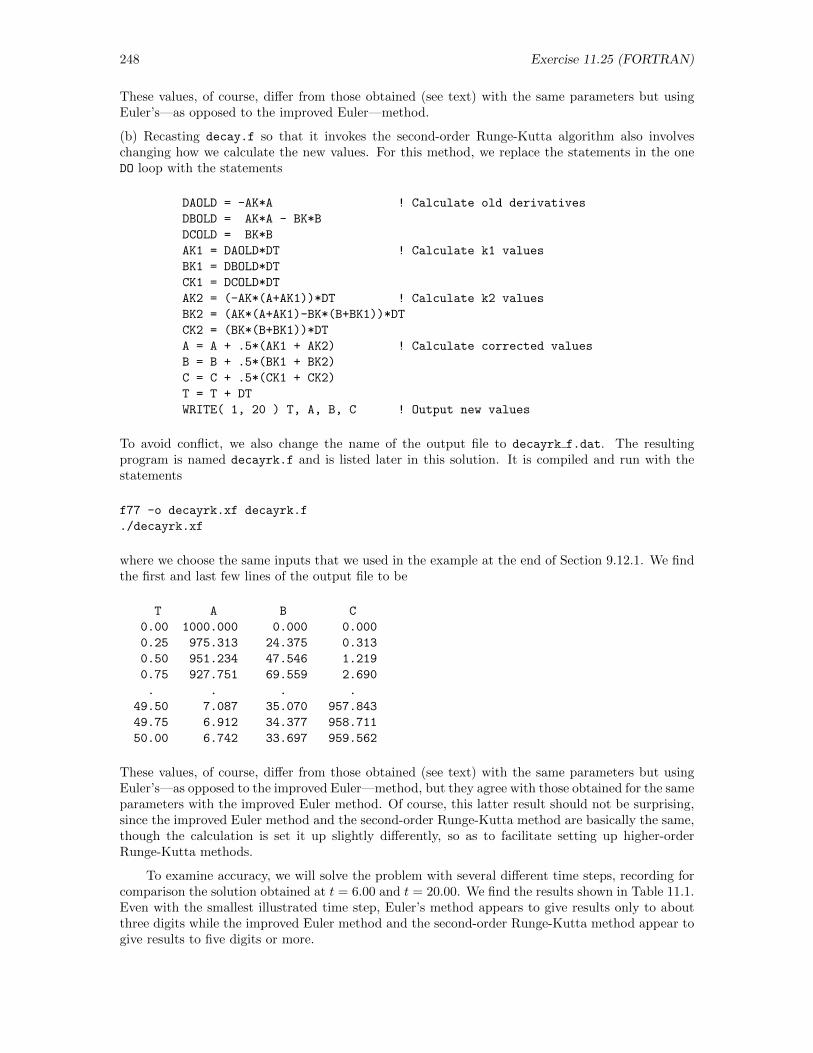
248 Exercise 11.25 (FORTRAN)
These values, of course, differ from those obtained (see text) with the same parameters but usingEuler’s—as opposed to the improved Euler—method.
(b) Recasting decay.f so that it invokes the second-order Runge-Kutta algorithm also involveschanging how we calculate the new values. For this method, we replace the statements in the oneDO loop with the statements
DAOLD = -AK*A ! Calculate old derivatives
DBOLD = AK*A - BK*B
DCOLD = BK*B
AK1 = DAOLD*DT ! Calculate k1 values
BK1 = DBOLD*DT
CK1 = DCOLD*DT
AK2 = (-AK*(A+AK1))*DT ! Calculate k2 values
BK2 = (AK*(A+AK1)-BK*(B+BK1))*DT
CK2 = (BK*(B+BK1))*DT
A = A + .5*(AK1 + AK2) ! Calculate corrected values
B = B + .5*(BK1 + BK2)
C = C + .5*(CK1 + CK2)
T = T + DT
WRITE( 1, 20 ) T, A, B, C ! Output new values
To avoid conflict, we also change the name of the output file to decayrk f.dat. The resultingprogram is named decayrk.f and is listed later in this solution. It is compiled and run with thestatements
f77 -o decayrk.xf decayrk.f
./decayrk.xf
where we choose the same inputs that we used in the example at the end of Section 9.12.1. We findthe first and last few lines of the output file to be
T A B C
0.00 1000.000 0.000 0.000
0.25 975.313 24.375 0.313
0.50 951.234 47.546 1.219
0.75 927.751 69.559 2.690
. . . .
49.50 7.087 35.070 957.843
49.75 6.912 34.377 958.711
50.00 6.742 33.697 959.562
These values, of course, differ from those obtained (see text) with the same parameters but usingEuler’s—as opposed to the improved Euler—method, but they agree with those obtained for the sameparameters with the improved Euler method. Of course, this latter result should not be surprising,since the improved Euler method and the second-order Runge-Kutta method are basically the same,though the calculation is set it up slightly differently, so as to facilitate setting up higher-orderRunge-Kutta methods.
To examine accuracy, we will solve the problem with several different time steps, recording forcomparison the solution obtained at t = 6.00 and t = 20.00. We find the results shown in Table 11.1.Even with the smallest illustrated time step, Euler’s method appears to give results only to aboutthree digits while the improved Euler method and the second-order Runge-Kutta method appear togive results to five digits or more.
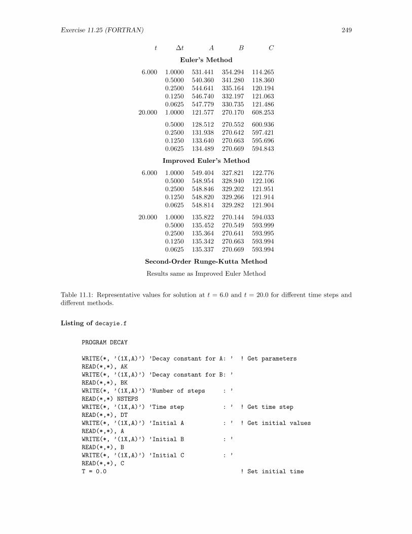
Exercise 11.25 (FORTRAN) 249
t ∆t A B C
Euler’s Method
6.000 1.0000 531.441 354.294 114.2650.5000 540.360 341.280 118.3600.2500 544.641 335.164 120.1940.1250 546.740 332.197 121.0630.0625 547.779 330.735 121.486
20.000 1.0000 121.577 270.170 608.253
0.5000 128.512 270.552 600.9360.2500 131.938 270.642 597.4210.1250 133.640 270.663 595.6960.0625 134.489 270.669 594.843
Improved Euler’s Method
6.000 1.0000 549.404 327.821 122.7760.5000 548.954 328.940 122.1060.2500 548.846 329.202 121.9510.1250 548.820 329.266 121.9140.0625 548.814 329.282 121.904
20.000 1.0000 135.822 270.144 594.0330.5000 135.452 270.549 593.9990.2500 135.364 270.641 593.9950.1250 135.342 270.663 593.9940.0625 135.337 270.669 593.994
Second-Order Runge-Kutta Method
Results same as Improved Euler Method
Table 11.1: Representative values for solution at t = 6.0 and t = 20.0 for different time steps anddifferent methods.
Listing of decayie.f
PROGRAM DECAY
WRITE(*, ’(1X,A)’) ’Decay constant for A: ’ ! Get parameters
READ(*,*), AK
WRITE(*, ’(1X,A)’) ’Decay constant for B: ’
READ(*,*), BK
WRITE(*, ’(1X,A)’) ’Number of steps : ’
READ(*,*) NSTEPS
WRITE(*, ’(1X,A)’) ’Time step : ’ ! Get time step
READ(*,*), DT
WRITE(*, ’(1X,A)’) ’Initial A : ’ ! Get initial values
READ(*,*), A
WRITE(*, ’(1X,A)’) ’Initial B : ’
READ(*,*), B
WRITE(*, ’(1X,A)’) ’Initial C : ’
READ(*,*), C
T = 0.0 ! Set initial time
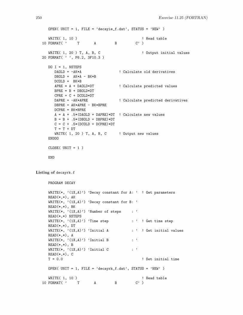
250 Exercise 11.25 (FORTRAN)
OPEN( UNIT = 1, FILE = ’decayie_f.dat’, STATUS = ’NEW’ )
WRITE( 1, 10 ) ! Head table
10 FORMAT( ’ T A B C’ )
WRITE( 1, 20 ) T, A, B, C ! Output initial values
20 FORMAT( ’ ’, F6.2, 3F10.3 )
DO I = 1, NSTEPS
DAOLD = -AK*A ! Calculate old derivatives
DBOLD = AK*A - BK*B
DCOLD = BK*B
APRE = A + DAOLD*DT ! Calculate predicted values
BPRE = B + DBOLD*DT
CPRE = C + DCOLD*DT
DAPRE = -AK*APRE ! Calculate predicted derivatives
DBPRE = AK*APRE - BK*BPRE
DCPRE = BK*BPRE
A = A + .5*(DAOLD + DAPRE)*DT ! Calculate new values
B = B + .5*(DBOLD + DBPRE)*DT
C = C + .5*(DCOLD + DCPRE)*DT
T = T + DT
WRITE( 1, 20 ) T, A, B, C ! Output new values
ENDDO
CLOSE( UNIT = 1 )
END
Listing of decayrk.f
PROGRAM DECAY
WRITE(*, ’(1X,A)’) ’Decay constant for A: ’ ! Get parameters
READ(*,*), AK
WRITE(*, ’(1X,A)’) ’Decay constant for B: ’
READ(*,*), BK
WRITE(*, ’(1X,A)’) ’Number of steps : ’
READ(*,*) NSTEPS
WRITE(*, ’(1X,A)’) ’Time step : ’ ! Get time step
READ(*,*), DT
WRITE(*, ’(1X,A)’) ’Initial A : ’ ! Get initial values
READ(*,*), A
WRITE(*, ’(1X,A)’) ’Initial B : ’
READ(*,*), B
WRITE(*, ’(1X,A)’) ’Initial C : ’
READ(*,*), C
T = 0.0 ! Set initial time
OPEN( UNIT = 1, FILE = ’decayrk_f.dat’, STATUS = ’NEW’ )
WRITE( 1, 10 ) ! Head table
10 FORMAT( ’ T A B C’ )
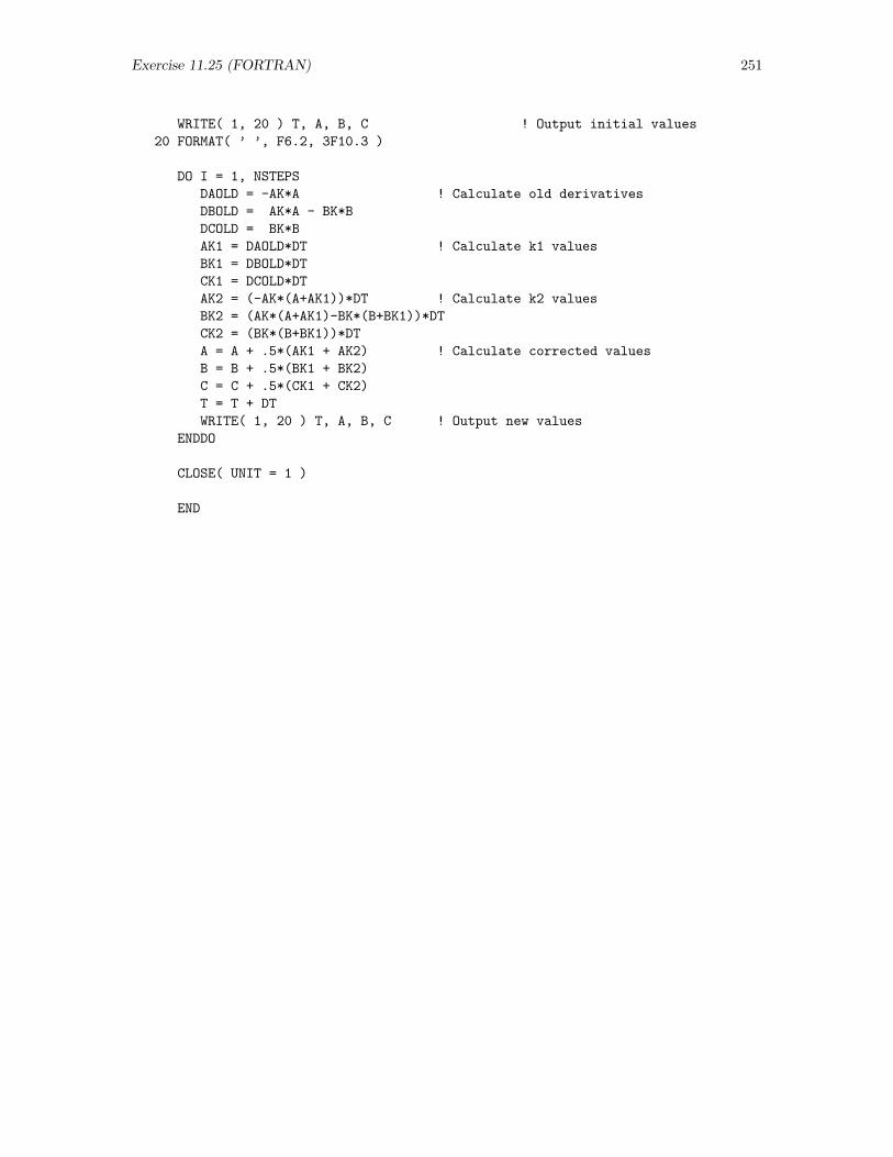
Exercise 11.25 (FORTRAN) 251
WRITE( 1, 20 ) T, A, B, C ! Output initial values
20 FORMAT( ’ ’, F6.2, 3F10.3 )
DO I = 1, NSTEPS
DAOLD = -AK*A ! Calculate old derivatives
DBOLD = AK*A - BK*B
DCOLD = BK*B
AK1 = DAOLD*DT ! Calculate k1 values
BK1 = DBOLD*DT
CK1 = DCOLD*DT
AK2 = (-AK*(A+AK1))*DT ! Calculate k2 values
BK2 = (AK*(A+AK1)-BK*(B+BK1))*DT
CK2 = (BK*(B+BK1))*DT
A = A + .5*(AK1 + AK2) ! Calculate corrected values
B = B + .5*(BK1 + BK2)
C = C + .5*(CK1 + CK2)
T = T + DT
WRITE( 1, 20 ) T, A, B, C ! Output new values
ENDDO
CLOSE( UNIT = 1 )
END
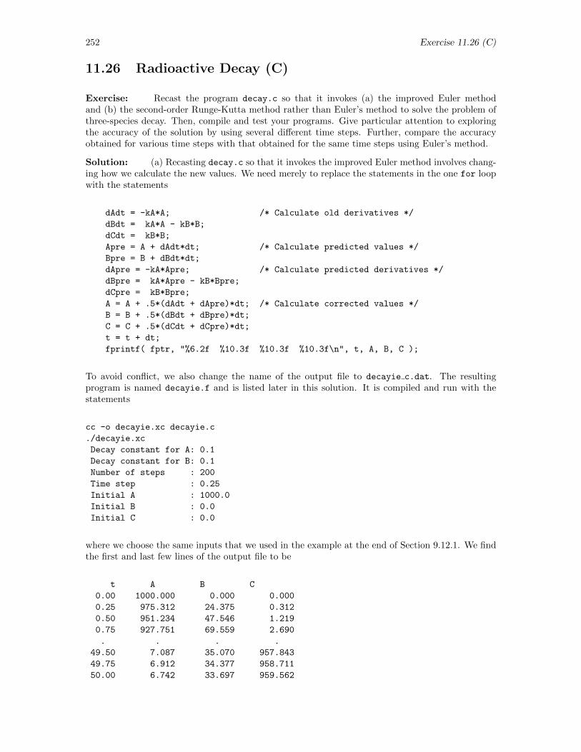
252 Exercise 11.26 (C)
11.26 Radioactive Decay (C)
Exercise: Recast the program decay.c so that it invokes (a) the improved Euler methodand (b) the second-order Runge-Kutta method rather than Euler’s method to solve the problem ofthree-species decay. Then, compile and test your programs. Give particular attention to exploringthe accuracy of the solution by using several different time steps. Further, compare the accuracyobtained for various time steps with that obtained for the same time steps using Euler’s method.
Solution: (a) Recasting decay.c so that it invokes the improved Euler method involves chang-ing how we calculate the new values. We need merely to replace the statements in the one for loopwith the statements
dAdt = -kA*A; /* Calculate old derivatives */
dBdt = kA*A - kB*B;
dCdt = kB*B;
Apre = A + dAdt*dt; /* Calculate predicted values */
Bpre = B + dBdt*dt;
dApre = -kA*Apre; /* Calculate predicted derivatives */
dBpre = kA*Apre - kB*Bpre;
dCpre = kB*Bpre;
A = A + .5*(dAdt + dApre)*dt; /* Calculate corrected values */
B = B + .5*(dBdt + dBpre)*dt;
C = C + .5*(dCdt + dCpre)*dt;
t = t + dt;
fprintf( fptr, "%6.2f %10.3f %10.3f %10.3f\n", t, A, B, C );
To avoid conflict, we also change the name of the output file to decayie c.dat. The resultingprogram is named decayie.f and is listed later in this solution. It is compiled and run with thestatements
cc -o decayie.xc decayie.c
./decayie.xc
Decay constant for A: 0.1
Decay constant for B: 0.1
Number of steps : 200
Time step : 0.25
Initial A : 1000.0
Initial B : 0.0
Initial C : 0.0
where we choose the same inputs that we used in the example at the end of Section 9.12.1. We findthe first and last few lines of the output file to be
t A B C
0.00 1000.000 0.000 0.000
0.25 975.312 24.375 0.312
0.50 951.234 47.546 1.219
0.75 927.751 69.559 2.690
. . . .
49.50 7.087 35.070 957.843
49.75 6.912 34.377 958.711
50.00 6.742 33.697 959.562
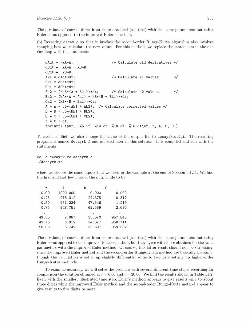
Exercise 11.26 (C) 253
These values, of course, differ from those obtained (see text) with the same parameters but usingEuler’s—as opposed to the improved Euler—method.
(b) Recasting decay.c so that it invokes the second-order Runge-Kutta algorithm also involveschanging how we calculate the new values. For this method, we replace the statements in the onefor loop with the statements
dAdt = -kA*A; /* Calculate old derivatives */
dBdt = kA*A - kB*B;
dCdt = kB*B;
Ak1 = dAdt*dt; /* Calculate k1 values */
Bk1 = dBdt*dt;
Ck1 = dCdt*dt;
Ak2 = (-kA*(A + Ak1))*dt; /* Calculate k2 values */
Bk2 = (kA*(A + Ak1) - kB*(B + Bk1))*dt;
Ck2 = (kB*(B + Bk1))*dt;
A = A + .5*(Ak1 + Ak2); /* Calculate corrected values */
B = B + .5*(Bk1 + Bk2);
C = C + .5*(Ck1 + Ck2);
t = t + dt;
fprintf( fptr, "%6.2f %10.3f %10.3f %10.3f\n", t, A, B, C );
To avoid conflict, we also change the name of the output file to decayrk c.dat. The resultingprogram is named decayrk.f and is listed later in this solution. It is compiled and run with thestatements
cc -o decayrk.xc decayrk.c
./decayrk.xc
where we choose the same inputs that we used in the example at the end of Section 9.12.1. We findthe first and last few lines of the output file to be
t A B C
0.00 1000.000 0.000 0.000
0.25 975.312 24.375 0.312
0.50 951.234 47.546 1.219
0.75 927.751 69.559 2.690
. . . .
49.50 7.087 35.070 957.843
49.75 6.912 34.377 958.711
50.00 6.742 33.697 959.562
These values, of course, differ from those obtained (see text) with the same parameters but usingEuler’s—as opposed to the improved Euler—method, but they agree with those obtained for the sameparameters with the improved Euler method. Of course, this latter result should not be surprising,since the improved Euler method and the second-order Runge-Kutta method are basically the same,though the calculation is set it up slightly differently, so as to facilitate setting up higher-orderRunge-Kutta methods.
To examine accuracy, we will solve the problem with several different time steps, recording forcomparison the solution obtained at t = 6.00 and t = 20.00. We find the results shown in Table 11.2.Even with the smallest illustrated time step, Euler’s method appears to give results only to aboutthree digits while the improved Euler method and the second-order Runge-Kutta method appear togive results to five digits or more.
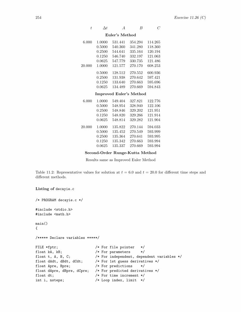
254 Exercise 11.26 (C)
t ∆t A B C
Euler’s Method
6.000 1.0000 531.441 354.294 114.2650.5000 540.360 341.280 118.3600.2500 544.641 335.164 120.1940.1250 546.740 332.197 121.0630.0625 547.779 330.735 121.486
20.000 1.0000 121.577 270.170 608.253
0.5000 128.512 270.552 600.9360.2500 131.938 270.642 597.4210.1250 133.640 270.663 595.6960.0625 134.489 270.669 594.843
Improved Euler’s Method
6.000 1.0000 549.404 327.821 122.7760.5000 548.954 328.940 122.1060.2500 548.846 329.202 121.9510.1250 548.820 329.266 121.9140.0625 548.814 329.282 121.904
20.000 1.0000 135.822 270.144 594.0330.5000 135.452 270.549 593.9990.2500 135.364 270.641 593.9950.1250 135.342 270.663 593.9940.0625 135.337 270.669 593.994
Second-Order Runge-Kutta Method
Results same as Improved Euler Method
Table 11.2: Representative values for solution at t = 6.0 and t = 20.0 for different time steps anddifferent methods.
Listing of decayie.c
/* PROGRAM decayie.c */
#include <stdio.h>
#include <math.h>
main()
/***** Declare variables *****/
FILE *fptr; /* For file pointer */
float kA, kB; /* For parameters */
float t, A, B, C; /* For independent, dependent variables */
float dAdt, dBdt, dCdt; /* For 1st guess derivatives */
float Apre, Bpre; /* For predictions */
float dApre, dBpre, dCpre; /* For predicted derivatives */
float dt; /* For time increment */
int i, nsteps; /* Loop index, limit */
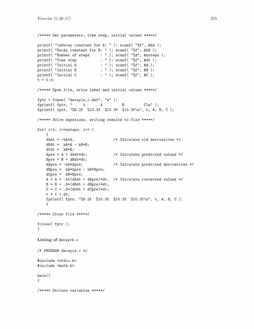
Exercise 11.26 (C) 255
/***** Get parameters, time step, initial values *****/
printf( "\nDecay constant for A: " ); scanf( "%f", &kA );
printf( "Decay constant for B: " ); scanf( "%f", &kB );
printf( "Number of steps : " ); scanf( "%d", &nsteps );
printf( "Time step : " ); scanf( "%f", &dt );
printf( "Initial A : " ); scanf( "%f", &A );
printf( "Initial B : " ); scanf( "%f", &B );
printf( "Initial C : " ); scanf( "%f", &C );
t = 0.0;
/***** Open file, write label and initial values *****/
fptr = fopen( "decayie_c.dat", "w" );
fprintf( fptr, " t A B C\n" );
fprintf( fptr, "%6.2f %10.3f %10.3f %10.3f\n", t, A, B, C );
/***** Solve equations, writing results to file *****/
for( i=1; i<=nsteps; i++ )
dAdt = -kA*A; /* Calculate old derivatives */
dBdt = kA*A - kB*B;
dCdt = kB*B;
Apre = A + dAdt*dt; /* Calculate predicted values */
Bpre = B + dBdt*dt;
dApre = -kA*Apre; /* Calculate predicted derivatives */
dBpre = kA*Apre - kB*Bpre;
dCpre = kB*Bpre;
A = A + .5*(dAdt + dApre)*dt; /* Calculate corrected values */
B = B + .5*(dBdt + dBpre)*dt;
C = C + .5*(dCdt + dCpre)*dt;
t = t + dt;
fprintf( fptr, "%6.2f %10.3f %10.3f %10.3f\n", t, A, B, C );
/***** Close file *****/
fclose( fptr );
Listing of decayrk.c
/* PROGRAM decayie.c */
#include <stdio.h>
#include <math.h>
main()
/***** Declare variables *****/
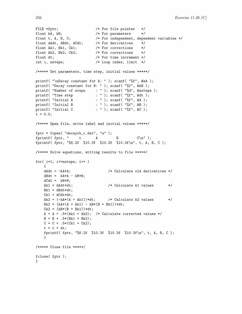
256 Exercise 11.26 (C)
FILE *fptr; /* For file pointer */
float kA, kB; /* For parameters */
float t, A, B, C; /* For independent, dependent variables */
float dAdt, dBdt, dCdt; /* For derivatives */
float Ak1, Bk1, Ck1; /* For corrections */
float Ak2, Bk2, Ck2; /* For corrections */
float dt; /* For time increment */
int i, nsteps; /* Loop index, limit */
/***** Get parameters, time step, initial values *****/
printf( "\nDecay constant for A: " ); scanf( "%f", &kA );
printf( "Decay constant for B: " ); scanf( "%f", &kB );
printf( "Number of steps : " ); scanf( "%d", &nsteps );
printf( "Time step : " ); scanf( "%f", &dt );
printf( "Initial A : " ); scanf( "%f", &A );
printf( "Initial B : " ); scanf( "%f", &B );
printf( "Initial C : " ); scanf( "%f", &C );
t = 0.0;
/***** Open file, write label and initial values *****/
fptr = fopen( "decayrk_c.dat", "w" );
fprintf( fptr, " t A B C\n" );
fprintf( fptr, "%6.2f %10.3f %10.3f %10.3f\n", t, A, B, C );
/***** Solve equations, writing results to file *****/
for( i=1; i<=nsteps; i++ )
dAdt = -kA*A; /* Calculate old derivatives */
dBdt = kA*A - kB*B;
dCdt = kB*B;
Ak1 = dAdt*dt; /* Calculate k1 values */
Bk1 = dBdt*dt;
Ck1 = dCdt*dt;
Ak2 = (-kA*(A + Ak1))*dt; /* Calculate k2 values */
Bk2 = (kA*(A + Ak1) - kB*(B + Bk1))*dt;
Ck2 = (kB*(B + Bk1))*dt;
A = A + .5*(Ak1 + Ak2); /* Calculate corrected values */
B = B + .5*(Bk1 + Bk2);
C = C + .5*(Ck1 + Ck2);
t = t + dt;
fprintf( fptr, "%6.2f %10.3f %10.3f %10.3f\n", t, A, B, C );
/***** Close file *****/
fclose( fptr );
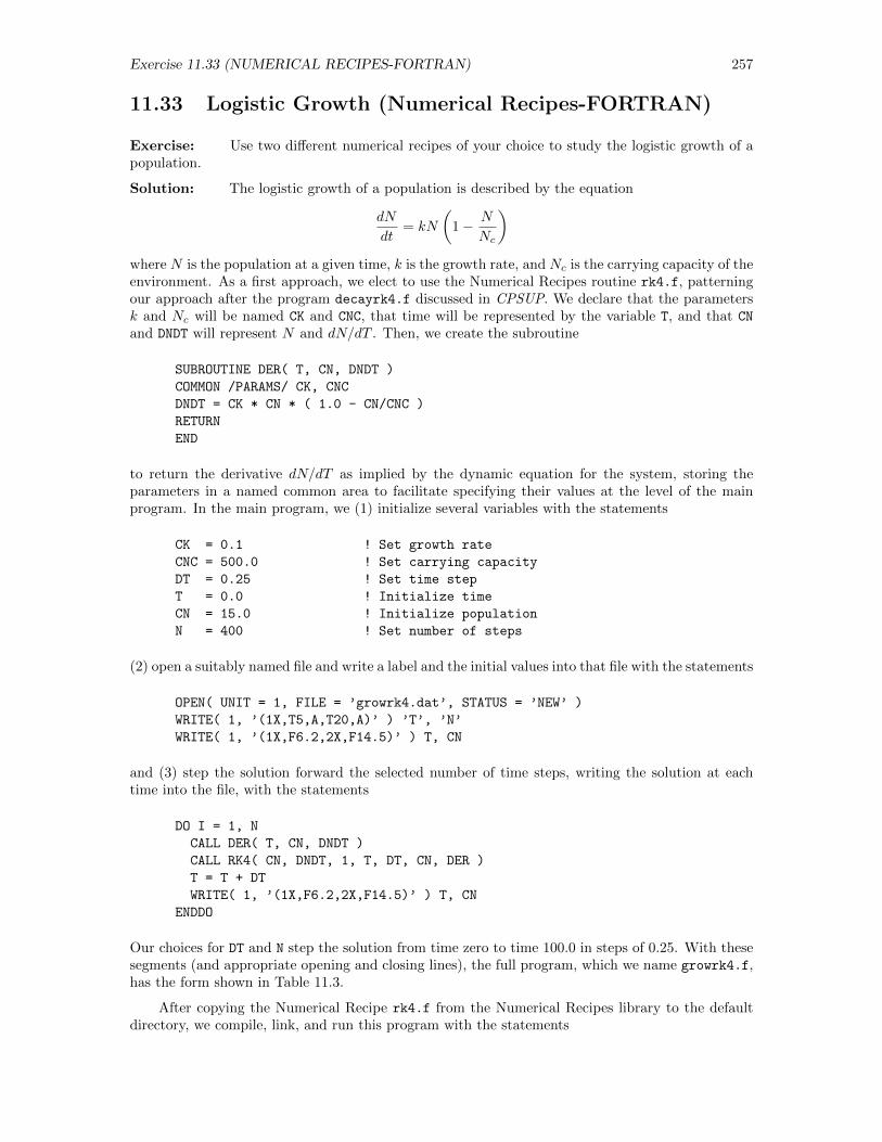
Exercise 11.33 (NUMERICAL RECIPES-FORTRAN) 257
11.33 Logistic Growth (Numerical Recipes-FORTRAN)
Exercise: Use two different numerical recipes of your choice to study the logistic growth of apopulation.
Solution: The logistic growth of a population is described by the equation
dN
dt= kN
(1− N
Nc
)where N is the population at a given time, k is the growth rate, and Nc is the carrying capacity of theenvironment. As a first approach, we elect to use the Numerical Recipes routine rk4.f, patterningour approach after the program decayrk4.f discussed in CPSUP. We declare that the parametersk and Nc will be named CK and CNC, that time will be represented by the variable T, and that CN
and DNDT will represent N and dN/dT . Then, we create the subroutine
SUBROUTINE DER( T, CN, DNDT )
COMMON /PARAMS/ CK, CNC
DNDT = CK * CN * ( 1.0 - CN/CNC )
RETURN
END
to return the derivative dN/dT as implied by the dynamic equation for the system, storing theparameters in a named common area to facilitate specifying their values at the level of the mainprogram. In the main program, we (1) initialize several variables with the statements
CK = 0.1 ! Set growth rate
CNC = 500.0 ! Set carrying capacity
DT = 0.25 ! Set time step
T = 0.0 ! Initialize time
CN = 15.0 ! Initialize population
N = 400 ! Set number of steps
(2) open a suitably named file and write a label and the initial values into that file with the statements
OPEN( UNIT = 1, FILE = ’growrk4.dat’, STATUS = ’NEW’ )
WRITE( 1, ’(1X,T5,A,T20,A)’ ) ’T’, ’N’
WRITE( 1, ’(1X,F6.2,2X,F14.5)’ ) T, CN
and (3) step the solution forward the selected number of time steps, writing the solution at eachtime into the file, with the statements
DO I = 1, N
CALL DER( T, CN, DNDT )
CALL RK4( CN, DNDT, 1, T, DT, CN, DER )
T = T + DT
WRITE( 1, ’(1X,F6.2,2X,F14.5)’ ) T, CN
ENDDO
Our choices for DT and N step the solution from time zero to time 100.0 in steps of 0.25. With thesesegments (and appropriate opening and closing lines), the full program, which we name growrk4.f,has the form shown in Table 11.3.
After copying the Numerical Recipe rk4.f from the Numerical Recipes library to the defaultdirectory, we compile, link, and run this program with the statements
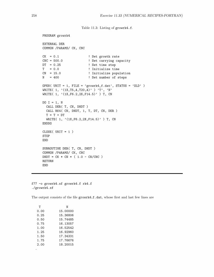
258 Exercise 11.33 (NUMERICAL RECIPES-FORTRAN)
Table 11.3: Listing of growrk4.f.
PROGRAM growrk4
EXTERNAL DER
COMMON /PARAMS/ CK, CNC
CK = 0.1 ! Set growth rate
CNC = 500.0 ! Set carrying capacity
DT = 0.25 ! Set time step
T = 0.0 ! Initialize time
CN = 15.0 ! Initialize population
N = 400 ! Set number of steps
OPEN( UNIT = 1, FILE = ’growrk4_f.dat’, STATUS = ’OLD’ )
WRITE( 1, ’(1X,T5,A,T20,A)’ ) ’T’, ’N’
WRITE( 1, ’(1X,F6.2,2X,F14.5)’ ) T, CN
DO I = 1, N
CALL DER( T, CN, DNDT )
CALL RK4( CN, DNDT, 1, T, DT, CN, DER )
T = T + DT
WRITE( 1, ’(1X,F6.2,2X,F14.5)’ ) T, CN
ENDDO
CLOSE( UNIT = 1 )
STOP
END
SUBROUTINE DER( T, CN, DNDT )
COMMON /PARAMS/ CK, CNC
DNDT = CK * CN * ( 1.0 - CN/CNC )
RETURN
END
f77 -o growrk4.xf growrk4.f rk4.f
./growrk4.xf
The output consists of the file growrk4 f.dat, whose first and last few lines are
T N
0.00 15.00000
0.25 15.36806
0.50 15.74485
0.75 16.13057
1.00 16.52542
1.25 16.92960
1.50 17.34331
1.75 17.76676
2.00 18.20015
.
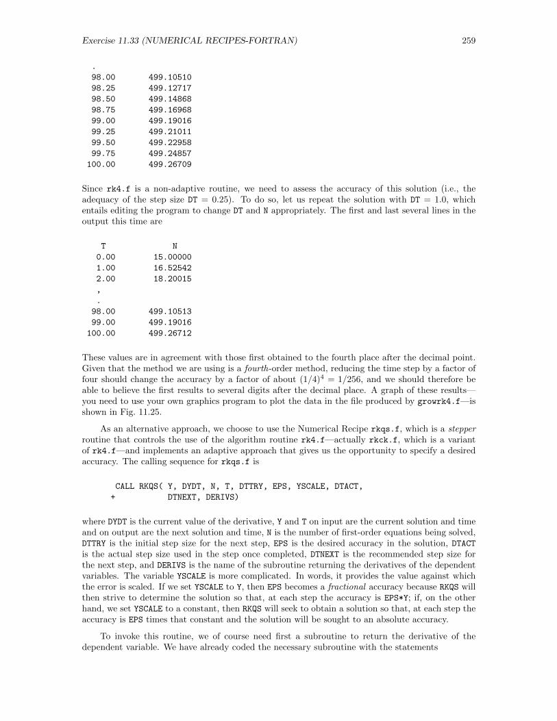
Exercise 11.33 (NUMERICAL RECIPES-FORTRAN) 259
.
98.00 499.10510
98.25 499.12717
98.50 499.14868
98.75 499.16968
99.00 499.19016
99.25 499.21011
99.50 499.22958
99.75 499.24857
100.00 499.26709
Since rk4.f is a non-adaptive routine, we need to assess the accuracy of this solution (i.e., theadequacy of the step size DT = 0.25). To do so, let us repeat the solution with DT = 1.0, whichentails editing the program to change DT and N appropriately. The first and last several lines in theoutput this time are
T N
0.00 15.00000
1.00 16.52542
2.00 18.20015
,
.
98.00 499.10513
99.00 499.19016
100.00 499.26712
These values are in agreement with those first obtained to the fourth place after the decimal point.Given that the method we are using is a fourth-order method, reducing the time step by a factor offour should change the accuracy by a factor of about (1/4)4 = 1/256, and we should therefore beable to believe the first results to several digits after the decimal place. A graph of these results—you need to use your own graphics program to plot the data in the file produced by growrk4.f—isshown in Fig. 11.25.
As an alternative approach, we choose to use the Numerical Recipe rkqs.f, which is a stepperroutine that controls the use of the algorithm routine rk4.f—actually rkck.f, which is a variantof rk4.f—and implements an adaptive approach that gives us the opportunity to specify a desiredaccuracy. The calling sequence for rkqs.f is
CALL RKQS( Y, DYDT, N, T, DTTRY, EPS, YSCALE, DTACT,
+ DTNEXT, DERIVS)
where DYDT is the current value of the derivative, Y and T on input are the current solution and timeand on output are the next solution and time, N is the number of first-order equations being solved,DTTRY is the initial step size for the next step, EPS is the desired accuracy in the solution, DTACTis the actual step size used in the step once completed, DTNEXT is the recommended step size forthe next step, and DERIVS is the name of the subroutine returning the derivatives of the dependentvariables. The variable YSCALE is more complicated. In words, it provides the value against whichthe error is scaled. If we set YSCALE to Y, then EPS becomes a fractional accuracy because RKQS willthen strive to determine the solution so that, at each step the accuracy is EPS*Y; if, on the otherhand, we set YSCALE to a constant, then RKQS will seek to obtain a solution so that, at each step theaccuracy is EPS times that constant and the solution will be sought to an absolute accuracy.
To invoke this routine, we of course need first a subroutine to return the derivative of thedependent variable. We have already coded the necessary subroutine with the statements
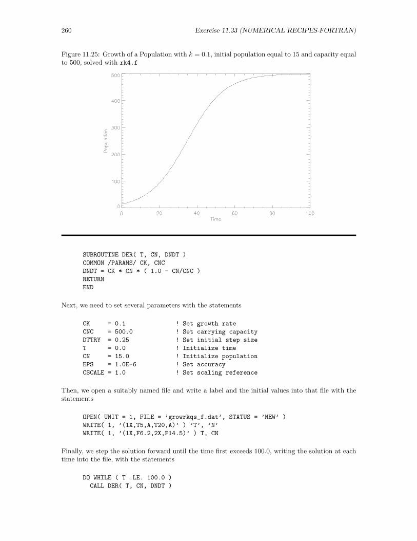
260 Exercise 11.33 (NUMERICAL RECIPES-FORTRAN)
Figure 11.25: Growth of a Population with k = 0.1, initial population equal to 15 and capacity equalto 500, solved with rk4.f
SUBROUTINE DER( T, CN, DNDT )
COMMON /PARAMS/ CK, CNC
DNDT = CK * CN * ( 1.0 - CN/CNC )
RETURN
END
Next, we need to set several parameters with the statements
CK = 0.1 ! Set growth rate
CNC = 500.0 ! Set carrying capacity
DTTRY = 0.25 ! Set initial step size
T = 0.0 ! Initialize time
CN = 15.0 ! Initialize population
EPS = 1.0E-6 ! Set accuracy
CSCALE = 1.0 ! Set scaling reference
Then, we open a suitably named file and write a label and the initial values into that file with thestatements
OPEN( UNIT = 1, FILE = ’growrkqs_f.dat’, STATUS = ’NEW’ )
WRITE( 1, ’(1X,T5,A,T20,A)’ ) ’T’, ’N’
WRITE( 1, ’(1X,F6.2,2X,F14.5)’ ) T, CN
Finally, we step the solution forward until the time first exceeds 100.0, writing the solution at eachtime into the file, with the statements
DO WHILE ( T .LE. 100.0 )
CALL DER( T, CN, DNDT )
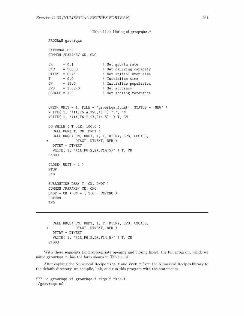
Exercise 11.33 (NUMERICAL RECIPES-FORTRAN) 261
Table 11.4: Listing of groqrqks.f.
PROGRAM growrqks
EXTERNAL DER
COMMON /PARAMS/ CK, CNC
CK = 0.1 ! Set growth rate
CNC = 500.0 ! Set carrying capacity
DTTRY = 0.25 ! Set initial step size
T = 0.0 ! Initialize time
CN = 15.0 ! Initialize population
EPS = 1.0E-6 ! Set accuracy
CSCALE = 1.0 ! Set scaling reference
OPEN( UNIT = 1, FILE = ’growrkqs_f.dat’, STATUS = ’NEW’ )
WRITE( 1, ’(1X,T5,A,T20,A)’ ) ’T’, ’N’
WRITE( 1, ’(1X,F6.2,2X,F14.5)’ ) T, CN
DO WHILE ( T .LE. 100.0 )
CALL DER( T, CN, DNDT )
CALL RKQS( CN, DNDT, 1, T, DTTRY, EPS, CSCALE,
+ DTACT, DTNEXT, DER )
DTTRY = DTNEXT
WRITE( 1, ’(1X,F6.2,2X,F14.5)’ ) T, CN
ENDDO
CLOSE( UNIT = 1 )
STOP
END
SUBROUTINE DER( T, CN, DNDT )
COMMON /PARAMS/ CK, CNC
DNDT = CK * CN * ( 1.0 - CN/CNC )
RETURN
END
CALL RKQS( CN, DNDT, 1, T, DTTRY, EPS, CSCALE,
+ DTACT, DTNEXT, DER )
DTTRY = DTNEXT
WRITE( 1, ’(1X,F6.2,2X,F14.5)’ ) T, CN
ENDDO
With these segments (and appropriate opening and closing lines), the full program, which wename growrkqs.f, has the form shown in Table 11.4.
After copying the Numerical Recipe rkqs.f and rkck.f from the Numerical Recipes library tothe default directory, we compile, link, and run this program with the statements
f77 -o growrkqs.xf growrkqs.f rkqs.f rkck.f
./growrkqs.xf
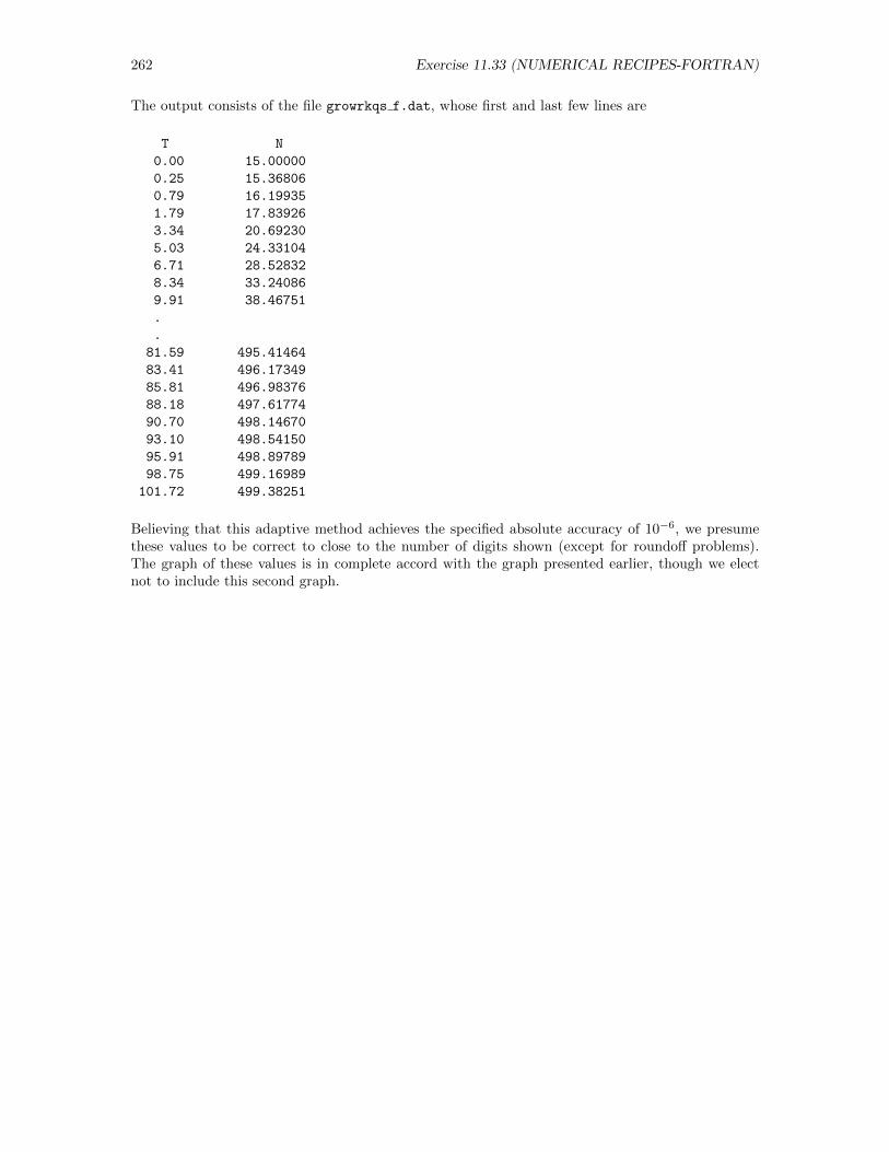
262 Exercise 11.33 (NUMERICAL RECIPES-FORTRAN)
The output consists of the file growrkqs f.dat, whose first and last few lines are
T N
0.00 15.00000
0.25 15.36806
0.79 16.19935
1.79 17.83926
3.34 20.69230
5.03 24.33104
6.71 28.52832
8.34 33.24086
9.91 38.46751
.
.
81.59 495.41464
83.41 496.17349
85.81 496.98376
88.18 497.61774
90.70 498.14670
93.10 498.54150
95.91 498.89789
98.75 499.16989
101.72 499.38251
Believing that this adaptive method achieves the specified absolute accuracy of 10−6, we presumethese values to be correct to close to the number of digits shown (except for roundoff problems).The graph of these values is in complete accord with the graph presented earlier, though we electnot to include this second graph.
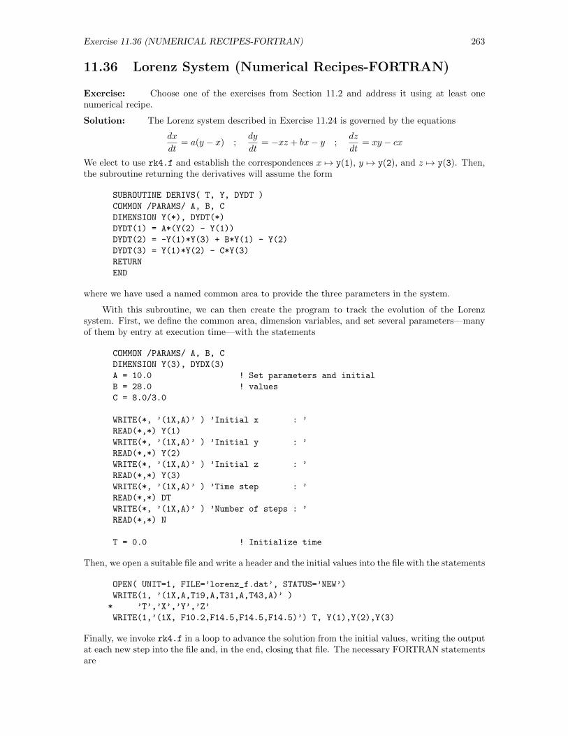
Exercise 11.36 (NUMERICAL RECIPES-FORTRAN) 263
11.36 Lorenz System (Numerical Recipes-FORTRAN)
Exercise: Choose one of the exercises from Section 11.2 and address it using at least onenumerical recipe.
Solution: The Lorenz system described in Exercise 11.24 is governed by the equations
dx
dt= a(y − x) ;
dy
dt= −xz + bx− y ;
dz
dt= xy − cx
We elect to use rk4.f and establish the correspondences x 7→ y(1), y 7→ y(2), and z 7→ y(3). Then,the subroutine returning the derivatives will assume the form
SUBROUTINE DERIVS( T, Y, DYDT )
COMMON /PARAMS/ A, B, C
DIMENSION Y(*), DYDT(*)
DYDT(1) = A*(Y(2) - Y(1))
DYDT(2) = -Y(1)*Y(3) + B*Y(1) - Y(2)
DYDT(3) = Y(1)*Y(2) - C*Y(3)
RETURN
END
where we have used a named common area to provide the three parameters in the system.
With this subroutine, we can then create the program to track the evolution of the Lorenzsystem. First, we define the common area, dimension variables, and set several parameters—manyof them by entry at execution time—with the statements
COMMON /PARAMS/ A, B, C
DIMENSION Y(3), DYDX(3)
A = 10.0 ! Set parameters and initial
B = 28.0 ! values
C = 8.0/3.0
WRITE(*, ’(1X,A)’ ) ’Initial x : ’
READ(*,*) Y(1)
WRITE(*, ’(1X,A)’ ) ’Initial y : ’
READ(*,*) Y(2)
WRITE(*, ’(1X,A)’ ) ’Initial z : ’
READ(*,*) Y(3)
WRITE(*, ’(1X,A)’ ) ’Time step : ’
READ(*,*) DT
WRITE(*, ’(1X,A)’ ) ’Number of steps : ’
READ(*,*) N
T = 0.0 ! Initialize time
Then, we open a suitable file and write a header and the initial values into the file with the statements
OPEN( UNIT=1, FILE=’lorenz_f.dat’, STATUS=’NEW’)
WRITE(1, ’(1X,A,T19,A,T31,A,T43,A)’ )
* ’T’,’X’,’Y’,’Z’
WRITE(1,’(1X, F10.2,F14.5,F14.5,F14.5)’) T, Y(1),Y(2),Y(3)
Finally, we invoke rk4.f in a loop to advance the solution from the initial values, writing the outputat each new step into the file and, in the end, closing that file. The necessary FORTRAN statementsare
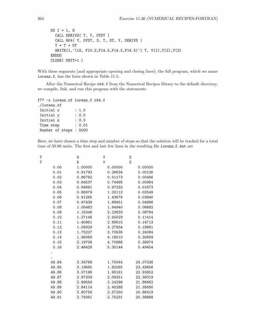
264 Exercise 11.36 (NUMERICAL RECIPES-FORTRAN)
DO I = 1, N
CALL DERIVS( T, Y, DYDT )
CALL RK4( Y, DYDT, 3, T, DT, Y, DERIVS )
T = T + DT
WRITE(1,’(1X, F10.2,F14.5,F14.5,F14.5)’) T, Y(1),Y(2),Y(3)
ENDDO
CLOSE( UNIT=1 )
With these segments (and appropriate opening and closing lines), the full program, which we namelorenz.f, has the form shown in Table 11.5.
After the Numerical Recipe rk4.f from the Numerical Recipes library to the default directory,we compile, link, and run this program with the statements
f77 -o lorenz.xf lorenz.f rk4.f
./lorenz.xf
Initial x : 1.0
Initial y : 0.0
Initial z : 0.0
Time step : 0.01
Number of steps : 5000
Here, we have chosen a time step and number of steps so that the solution will be tracked for a totaltime of 50.00 units. The first and last few lines in the resulting file lorenz f.dat are
T X Y Z
T X Y Z
0.00 1.00000 0.00000 0.00000
0.01 0.91793 0.26634 0.00126
0.02 0.86792 0.51173 0.00466
0.03 0.84537 0.74465 0.00984
0.04 0.84681 0.97232 0.01673
0.05 0.86979 1.20112 0.02549
0.06 0.91265 1.43676 0.03640
0.07 0.97439 1.68451 0.04996
0.08 1.05463 1.94940 0.06682
0.09 1.15346 2.23633 0.08784
0.10 1.27146 2.55023 0.11414
0.11 1.40961 2.89615 0.14713
0.12 1.56929 3.27934 0.18861
0.13 1.75227 3.70535 0.24084
0.14 1.96069 4.18010 0.30669
0.15 2.19706 4.70988 0.38974
0.16 2.46428 5.30144 0.49454
.
.
49.84 3.34768 1.70044 24.07326
49.85 3.19665 1.82065 23.49656
49.86 3.07196 1.95161 22.93652
49.87 2.97209 2.09251 22.39319
49.88 2.89559 2.24296 21.86662
49.89 2.84114 2.40288 21.35690
49.90 2.80756 2.57250 20.86419
49.91 2.79381 2.75231 20.38868
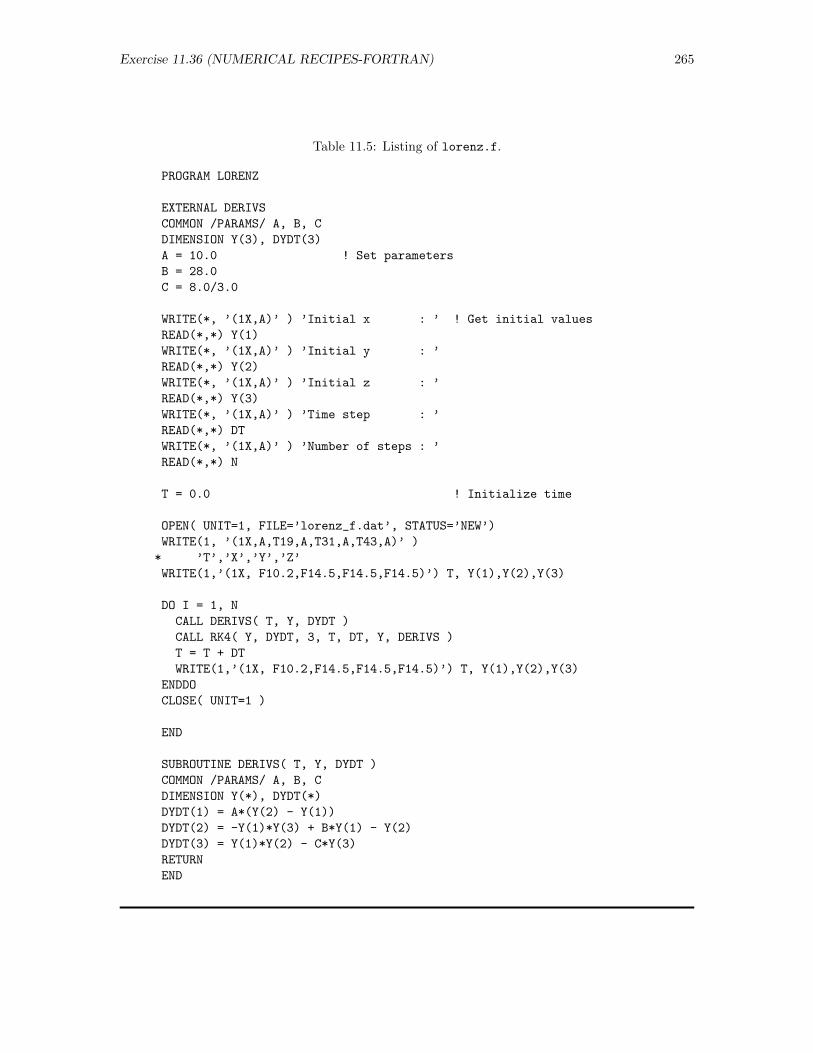
Exercise 11.36 (NUMERICAL RECIPES-FORTRAN) 265
Table 11.5: Listing of lorenz.f.
PROGRAM LORENZ
EXTERNAL DERIVS
COMMON /PARAMS/ A, B, C
DIMENSION Y(3), DYDT(3)
A = 10.0 ! Set parameters
B = 28.0
C = 8.0/3.0
WRITE(*, ’(1X,A)’ ) ’Initial x : ’ ! Get initial values
READ(*,*) Y(1)
WRITE(*, ’(1X,A)’ ) ’Initial y : ’
READ(*,*) Y(2)
WRITE(*, ’(1X,A)’ ) ’Initial z : ’
READ(*,*) Y(3)
WRITE(*, ’(1X,A)’ ) ’Time step : ’
READ(*,*) DT
WRITE(*, ’(1X,A)’ ) ’Number of steps : ’
READ(*,*) N
T = 0.0 ! Initialize time
OPEN( UNIT=1, FILE=’lorenz_f.dat’, STATUS=’NEW’)
WRITE(1, ’(1X,A,T19,A,T31,A,T43,A)’ )
* ’T’,’X’,’Y’,’Z’
WRITE(1,’(1X, F10.2,F14.5,F14.5,F14.5)’) T, Y(1),Y(2),Y(3)
DO I = 1, N
CALL DERIVS( T, Y, DYDT )
CALL RK4( Y, DYDT, 3, T, DT, Y, DERIVS )
T = T + DT
WRITE(1,’(1X, F10.2,F14.5,F14.5,F14.5)’) T, Y(1),Y(2),Y(3)
ENDDO
CLOSE( UNIT=1 )
END
SUBROUTINE DERIVS( T, Y, DYDT )
COMMON /PARAMS/ A, B, C
DIMENSION Y(*), DYDT(*)
DYDT(1) = A*(Y(2) - Y(1))
DYDT(2) = -Y(1)*Y(3) + B*Y(1) - Y(2)
DYDT(3) = Y(1)*Y(2) - C*Y(3)
RETURN
END
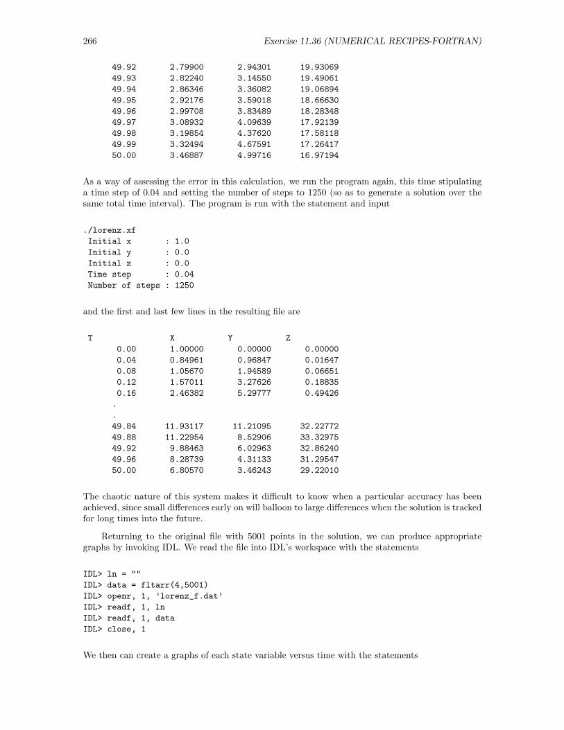
266 Exercise 11.36 (NUMERICAL RECIPES-FORTRAN)
49.92 2.79900 2.94301 19.93069
49.93 2.82240 3.14550 19.49061
49.94 2.86346 3.36082 19.06894
49.95 2.92176 3.59018 18.66630
49.96 2.99708 3.83489 18.28348
49.97 3.08932 4.09639 17.92139
49.98 3.19854 4.37620 17.58118
49.99 3.32494 4.67591 17.26417
50.00 3.46887 4.99716 16.97194
As a way of assessing the error in this calculation, we run the program again, this time stipulatinga time step of 0.04 and setting the number of steps to 1250 (so as to generate a solution over thesame total time interval). The program is run with the statement and input
./lorenz.xf
Initial x : 1.0
Initial y : 0.0
Initial z : 0.0
Time step : 0.04
Number of steps : 1250
and the first and last few lines in the resulting file are
T X Y Z
0.00 1.00000 0.00000 0.00000
0.04 0.84961 0.96847 0.01647
0.08 1.05670 1.94589 0.06651
0.12 1.57011 3.27626 0.18835
0.16 2.46382 5.29777 0.49426
.
.
49.84 11.93117 11.21095 32.22772
49.88 11.22954 8.52906 33.32975
49.92 9.88463 6.02963 32.86240
49.96 8.28739 4.31133 31.29547
50.00 6.80570 3.46243 29.22010
The chaotic nature of this system makes it difficult to know when a particular accuracy has beenachieved, since small differences early on will balloon to large differences when the solution is trackedfor long times into the future.
Returning to the original file with 5001 points in the solution, we can produce appropriategraphs by invoking IDL. We read the file into IDL’s workspace with the statements
IDL> ln = ""
IDL> data = fltarr(4,5001)
IDL> openr, 1, ’lorenz_f.dat’
IDL> readf, 1, ln
IDL> readf, 1, data
IDL> close, 1
We then can create a graphs of each state variable versus time with the statements
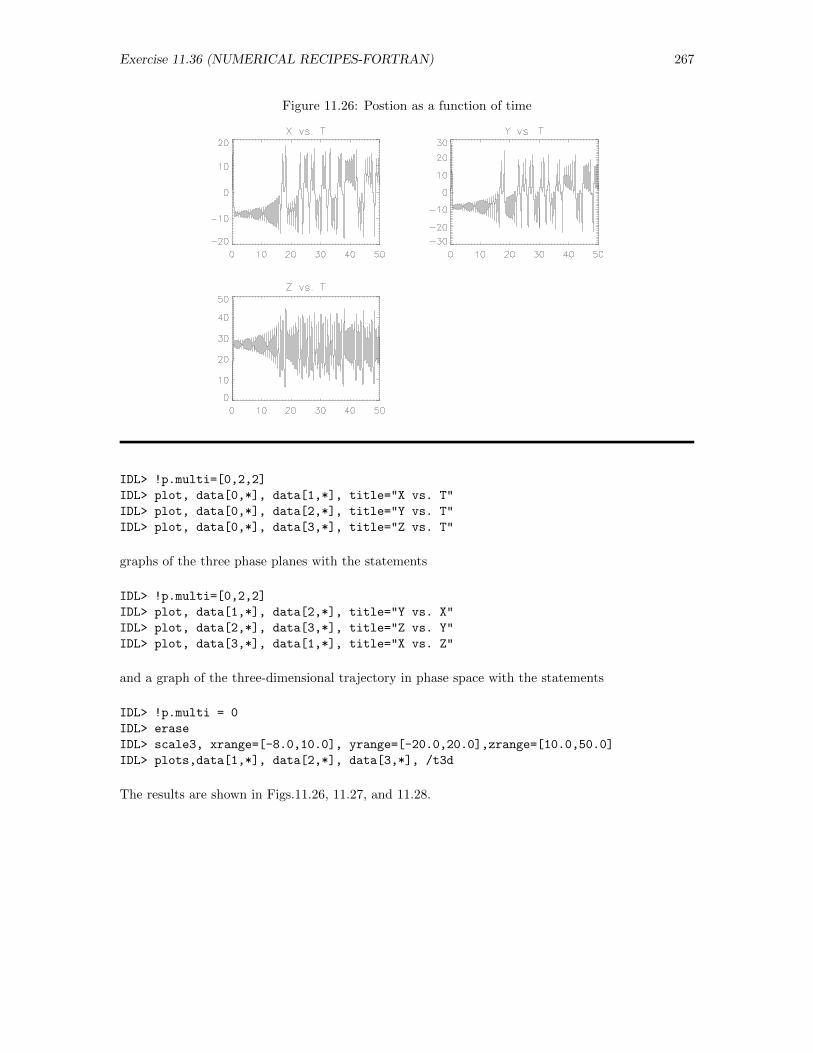
Exercise 11.36 (NUMERICAL RECIPES-FORTRAN) 267
Figure 11.26: Postion as a function of time
IDL> !p.multi=[0,2,2]
IDL> plot, data[0,*], data[1,*], title="X vs. T"
IDL> plot, data[0,*], data[2,*], title="Y vs. T"
IDL> plot, data[0,*], data[3,*], title="Z vs. T"
graphs of the three phase planes with the statements
IDL> !p.multi=[0,2,2]
IDL> plot, data[1,*], data[2,*], title="Y vs. X"
IDL> plot, data[2,*], data[3,*], title="Z vs. Y"
IDL> plot, data[3,*], data[1,*], title="X vs. Z"
and a graph of the three-dimensional trajectory in phase space with the statements
IDL> !p.multi = 0
IDL> erase
IDL> scale3, xrange=[-8.0,10.0], yrange=[-20.0,20.0],zrange=[10.0,50.0]
IDL> plots,data[1,*], data[2,*], data[3,*], /t3d
The results are shown in Figs.11.26, 11.27, and 11.28.
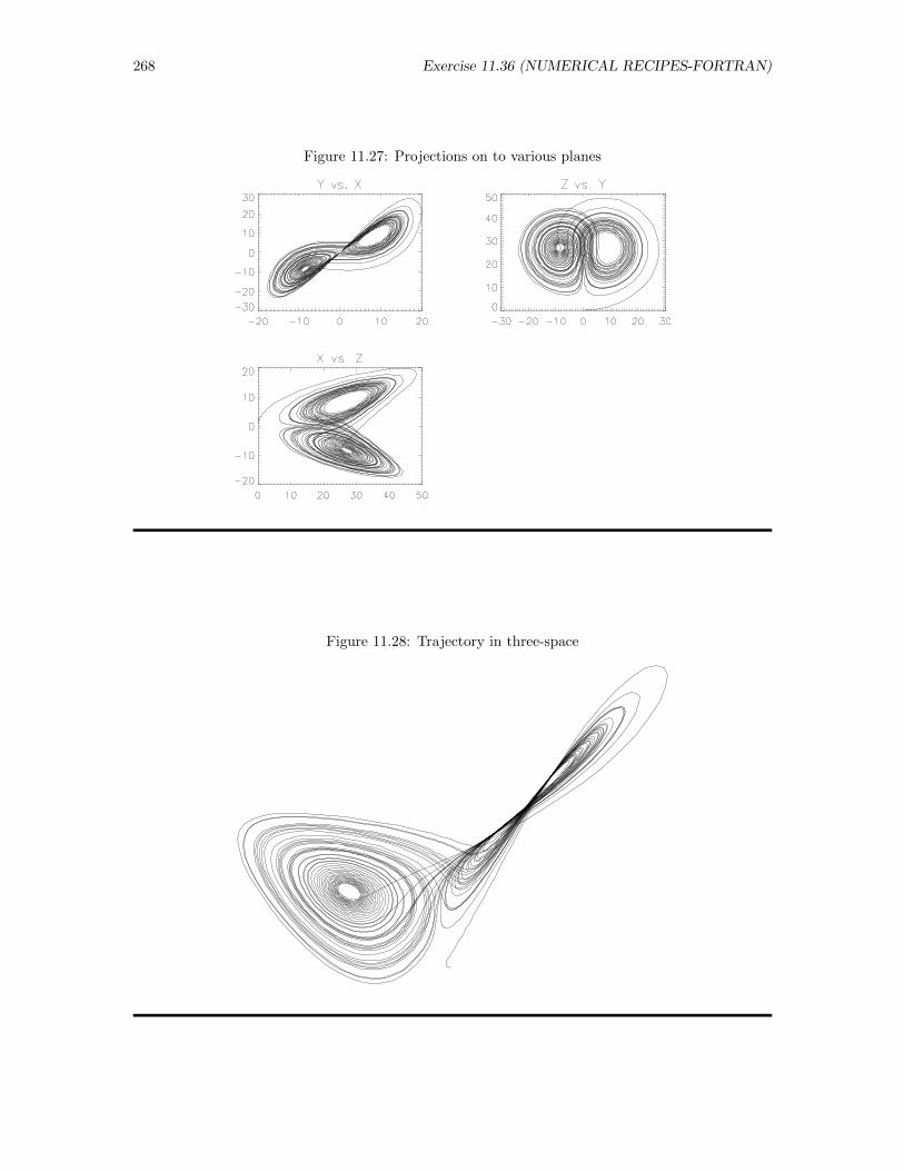
268 Exercise 11.36 (NUMERICAL RECIPES-FORTRAN)
Figure 11.27: Projections on to various planes
Figure 11.28: Trajectory in three-space
Exercise 11.33 (NUMERICAL RECIPES-C) 269
11.33 Logistic Growth (Numerical Recipes-C)
Exercise: Use two different numerical recipes of your choice to study the logistic growth of apopulation.
Solution: The logistic growth of a population is described by the equation
dN
dt= kN
(1− N
Nc
)where N is the population at a given time, k is the growth rate, and Nc is the carrying capacityof the environment. As a first approach, we elect to use the Numerical Recipes routine rk4.c,patterning our approach after the program decayrk4.c discussed in CPSUP. We declare that theparameters k and Nc will be named k and Nc, that time will be represented by the variable t, andthat N[1] and dNdt[1] will represent N and dN/dT . Further, we note that we must define N anddNdt as arrays with dimension two (because indices in C start at zero), even though we have only asingle equation to solve. Then, we create the procedure
void derivs( float t, float N[], float dNdt[] )
float k=0.1, Nc=500.0;
dNdt[1] = k * N[1] * ( 1.0 - N[1]/Nc );
to return the derivative dN/dT as implied by the dynamic equation for the system, hard codingvalues of the parameters in the routine itself. In the main program, we (1) declare and initializeseveral variables with the statements
int i, n; /* For loop index, number of steps */
float dt, t; /* For time step, time */
float N[2], dNdt[2]; /* For N, and dN/dt */
FILE *fptr; /* For output file */
N[1] = 15.0; /* Initialize population */
t = 0.0; /* Initialize time */
dt = 0.25; /* Set time step */
n = 400; /* Set number of steps */
(2) open a suitably named file and write a label and the initial values into that file with the statements
fptr = fopen( "growrk4_c.dat", "w" );
fprintf( fptr, " T N\n" );
fprintf( fptr, " %12.4f %12.4f\n", t, N[1] );
and (3) step the solution forward the selected number of time steps, writing the solution at eachtime into the file, with the statements
for ( i=0; i<n; i++ )
derivs( t, N, dNdt );
t = t + dt;
rk4( N, dNdt, 1, t, dt, N, derivs );
fprintf( fptr, " %12.4f %12.4f\n", t, N[1] );
fclose(fptr);
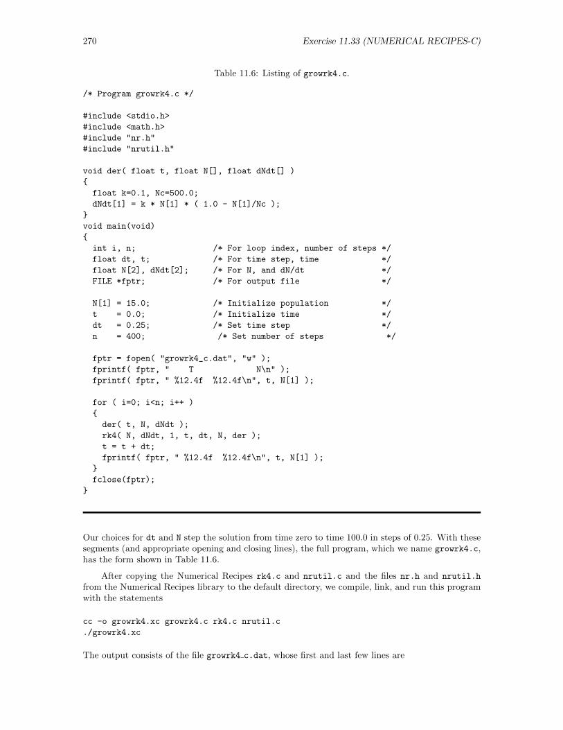
270 Exercise 11.33 (NUMERICAL RECIPES-C)
Table 11.6: Listing of growrk4.c.
/* Program growrk4.c */
#include <stdio.h>
#include <math.h>
#include "nr.h"
#include "nrutil.h"
void der( float t, float N[], float dNdt[] )
float k=0.1, Nc=500.0;
dNdt[1] = k * N[1] * ( 1.0 - N[1]/Nc );
void main(void)
int i, n; /* For loop index, number of steps */
float dt, t; /* For time step, time */
float N[2], dNdt[2]; /* For N, and dN/dt */
FILE *fptr; /* For output file */
N[1] = 15.0; /* Initialize population */
t = 0.0; /* Initialize time */
dt = 0.25; /* Set time step */
n = 400; /* Set number of steps */
fptr = fopen( "growrk4_c.dat", "w" );
fprintf( fptr, " T N\n" );
fprintf( fptr, " %12.4f %12.4f\n", t, N[1] );
for ( i=0; i<n; i++ )
der( t, N, dNdt );
rk4( N, dNdt, 1, t, dt, N, der );
t = t + dt;
fprintf( fptr, " %12.4f %12.4f\n", t, N[1] );
fclose(fptr);
Our choices for dt and N step the solution from time zero to time 100.0 in steps of 0.25. With thesesegments (and appropriate opening and closing lines), the full program, which we name growrk4.c,has the form shown in Table 11.6.
After copying the Numerical Recipes rk4.c and nrutil.c and the files nr.h and nrutil.h
from the Numerical Recipes library to the default directory, we compile, link, and run this programwith the statements
cc -o growrk4.xc growrk4.c rk4.c nrutil.c
./growrk4.xc
The output consists of the file growrk4 c.dat, whose first and last few lines are
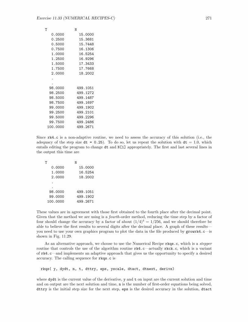
Exercise 11.33 (NUMERICAL RECIPES-C) 271
T N
0.0000 15.0000
0.2500 15.3681
0.5000 15.7448
0.7500 16.1306
1.0000 16.5254
1.2500 16.9296
1.5000 17.3433
1.7500 17.7668
2.0000 18.2002
.
.
98.0000 499.1051
98.2500 499.1272
98.5000 499.1487
98.7500 499.1697
99.0000 499.1902
99.2500 499.2101
99.5000 499.2296
99.7500 499.2486
100.0000 499.2671
Since rk4.c is a non-adaptive routine, we need to assess the accuracy of this solution (i.e., theadequacy of the step size dt = 0.25). To do so, let us repeat the solution with dt = 1.0, whichentails editing the program to change dt and N[1] appropriately. The first and last several lines inthe output this time are
T N
0.0000 15.0000
1.0000 16.5254
2.0000 18.2002
.
.
98.0000 499.1051
99.0000 499.1902
100.0000 499.2671
These values are in agreement with those first obtained to the fourth place after the decimal point.Given that the method we are using is a fourth-order method, reducing the time step by a factor offour should change the accuracy by a factor of about (1/4)4 = 1/256, and we should therefore beable to believe the first results to several digits after the decimal place. A graph of these results—you need to use your own graphics program to plot the data in the file produced by growrk4.c—isshown in Fig. 11.29.
As an alternative approach, we choose to use the Numerical Recipe rkqs.c, which is a stepperroutine that controls the use of the algorithm routine rk4.c—actually rkck.c, which is a variantof rk4.c—and implements an adaptive approach that gives us the opportunity to specify a desiredaccuracy. The calling sequence for rkqs.c is
rkqs( y, dydt, n, t, dttry, eps, yscale, dtact, dtnext, derivs)
where dydt is the current value of the derivative, y and t on input are the current solution and timeand on output are the next solution and time, n is the number of first-order equations being solved,dttry is the initial step size for the next step, eps is the desired accuracy in the solution, dtact
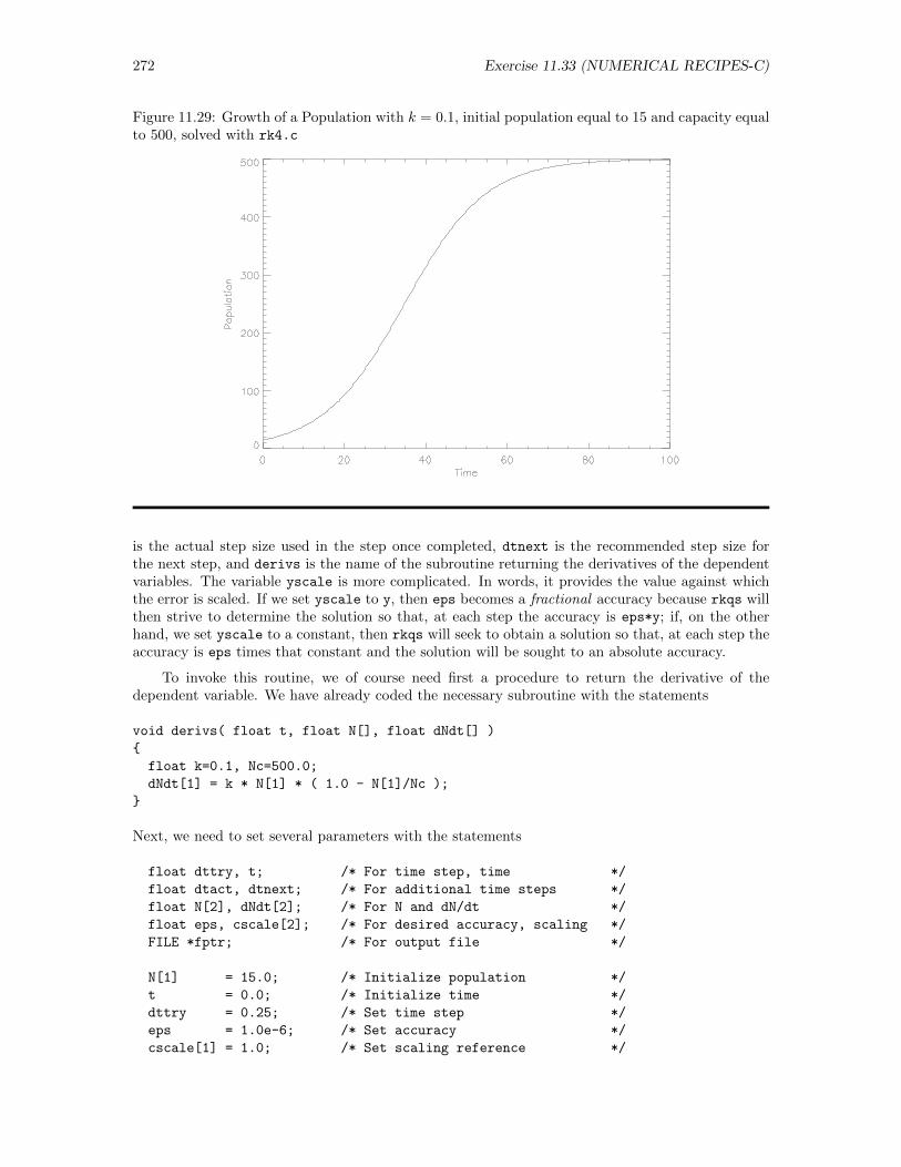
272 Exercise 11.33 (NUMERICAL RECIPES-C)
Figure 11.29: Growth of a Population with k = 0.1, initial population equal to 15 and capacity equalto 500, solved with rk4.c
is the actual step size used in the step once completed, dtnext is the recommended step size forthe next step, and derivs is the name of the subroutine returning the derivatives of the dependentvariables. The variable yscale is more complicated. In words, it provides the value against whichthe error is scaled. If we set yscale to y, then eps becomes a fractional accuracy because rkqs willthen strive to determine the solution so that, at each step the accuracy is eps*y; if, on the otherhand, we set yscale to a constant, then rkqs will seek to obtain a solution so that, at each step theaccuracy is eps times that constant and the solution will be sought to an absolute accuracy.
To invoke this routine, we of course need first a procedure to return the derivative of thedependent variable. We have already coded the necessary subroutine with the statements
void derivs( float t, float N[], float dNdt[] )
float k=0.1, Nc=500.0;
dNdt[1] = k * N[1] * ( 1.0 - N[1]/Nc );
Next, we need to set several parameters with the statements
float dttry, t; /* For time step, time */
float dtact, dtnext; /* For additional time steps */
float N[2], dNdt[2]; /* For N and dN/dt */
float eps, cscale[2]; /* For desired accuracy, scaling */
FILE *fptr; /* For output file */
N[1] = 15.0; /* Initialize population */
t = 0.0; /* Initialize time */
dttry = 0.25; /* Set time step */
eps = 1.0e-6; /* Set accuracy */
cscale[1] = 1.0; /* Set scaling reference */
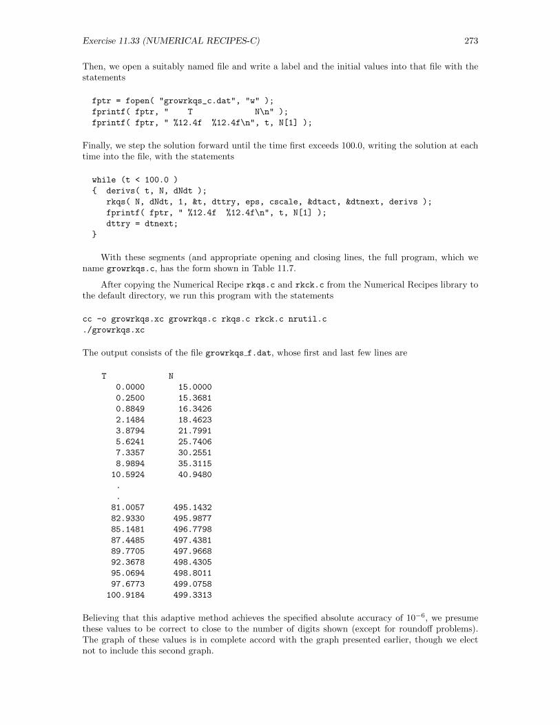
Exercise 11.33 (NUMERICAL RECIPES-C) 273
Then, we open a suitably named file and write a label and the initial values into that file with thestatements
fptr = fopen( "growrkqs_c.dat", "w" );
fprintf( fptr, " T N\n" );
fprintf( fptr, " %12.4f %12.4f\n", t, N[1] );
Finally, we step the solution forward until the time first exceeds 100.0, writing the solution at eachtime into the file, with the statements
while (t < 100.0 )
derivs( t, N, dNdt );
rkqs( N, dNdt, 1, &t, dttry, eps, cscale, &dtact, &dtnext, derivs );
fprintf( fptr, " %12.4f %12.4f\n", t, N[1] );
dttry = dtnext;
With these segments (and appropriate opening and closing lines, the full program, which wename growrkqs.c, has the form shown in Table 11.7.
After copying the Numerical Recipe rkqs.c and rkck.c from the Numerical Recipes library tothe default directory, we run this program with the statements
cc -o growrkqs.xc growrkqs.c rkqs.c rkck.c nrutil.c
./growrkqs.xc
The output consists of the file growrkqs f.dat, whose first and last few lines are
T N
0.0000 15.0000
0.2500 15.3681
0.8849 16.3426
2.1484 18.4623
3.8794 21.7991
5.6241 25.7406
7.3357 30.2551
8.9894 35.3115
10.5924 40.9480
.
.
81.0057 495.1432
82.9330 495.9877
85.1481 496.7798
87.4485 497.4381
89.7705 497.9668
92.3678 498.4305
95.0694 498.8011
97.6773 499.0758
100.9184 499.3313
Believing that this adaptive method achieves the specified absolute accuracy of 10−6, we presumethese values to be correct to close to the number of digits shown (except for roundoff problems).The graph of these values is in complete accord with the graph presented earlier, though we electnot to include this second graph.
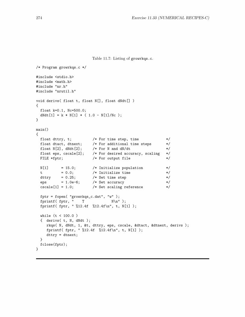
274 Exercise 11.33 (NUMERICAL RECIPES-C)
Table 11.7: Listing of growrkqs.c.
/* Program growrkqs.c */
#include <stdio.h>
#include <math.h>
#include "nr.h"
#include "nrutil.h"
void derivs( float t, float N[], float dNdt[] )
float k=0.1, Nc=500.0;
dNdt[1] = k * N[1] * ( 1.0 - N[1]/Nc );
main()
float dttry, t; /* For time step, time */
float dtact, dtnext; /* For additional time steps */
float N[2], dNdt[2]; /* For N and dN/dt */
float eps, cscale[2]; /* For desired accuracy, scaling */
FILE *fptr; /* For output file */
N[1] = 15.0; /* Initialize population */
t = 0.0; /* Initialize time */
dttry = 0.25; /* Set time step */
eps = 1.0e-6; /* Set accuracy */
cscale[1] = 1.0; /* Set scaling reference */
fptr = fopen( "growrkqs_c.dat", "w" );
fprintf( fptr, " T N\n" );
fprintf( fptr, " %12.4f %12.4f\n", t, N[1] );
while (t < 100.0 )
derivs( t, N, dNdt );
rkqs( N, dNdt, 1, &t, dttry, eps, cscale, &dtact, &dtnext, derivs );
fprintf( fptr, " %12.4f %12.4f\n", t, N[1] );
dttry = dtnext;
fclose(fptr);
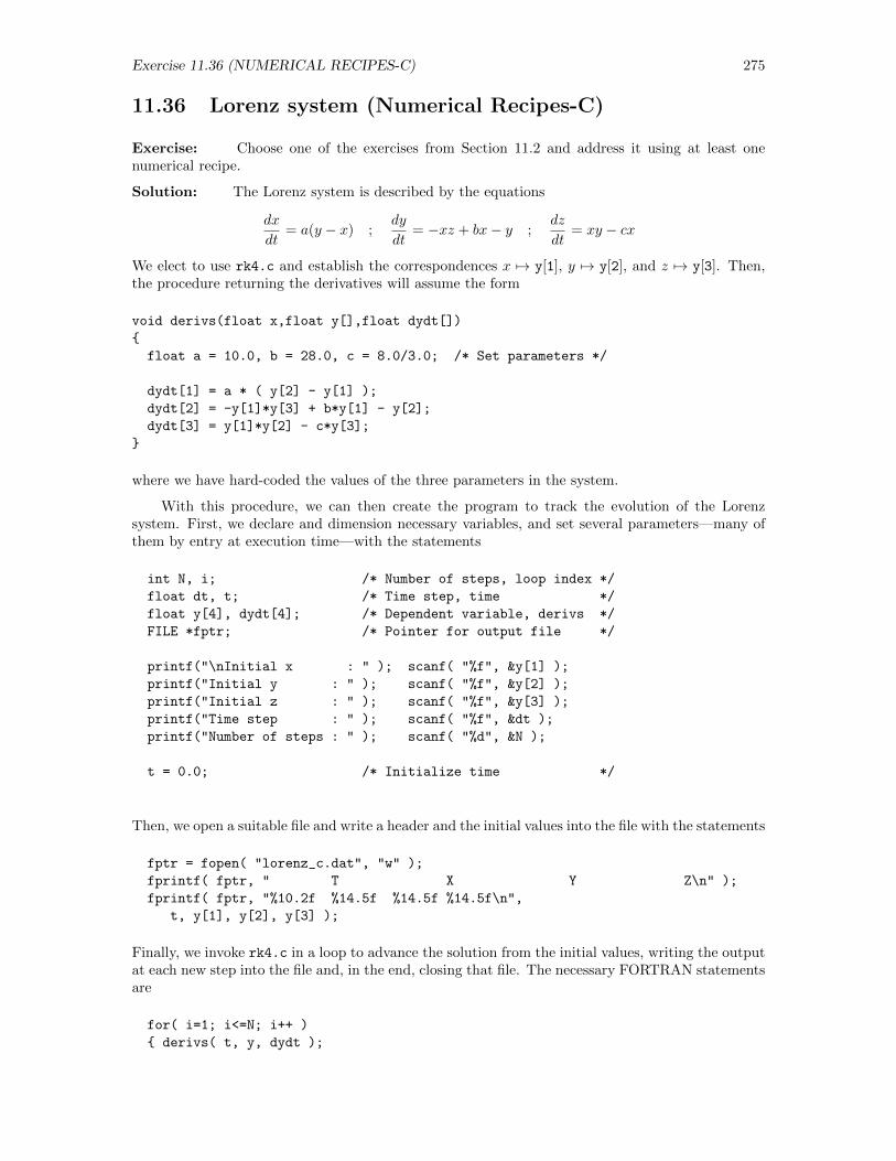
Exercise 11.36 (NUMERICAL RECIPES-C) 275
11.36 Lorenz system (Numerical Recipes-C)
Exercise: Choose one of the exercises from Section 11.2 and address it using at least onenumerical recipe.
Solution: The Lorenz system is described by the equations
dx
dt= a(y − x) ;
dy
dt= −xz + bx− y ;
dz
dt= xy − cx
We elect to use rk4.c and establish the correspondences x 7→ y[1], y 7→ y[2], and z 7→ y[3]. Then,the procedure returning the derivatives will assume the form
void derivs(float x,float y[],float dydt[])
float a = 10.0, b = 28.0, c = 8.0/3.0; /* Set parameters */
dydt[1] = a * ( y[2] - y[1] );
dydt[2] = -y[1]*y[3] + b*y[1] - y[2];
dydt[3] = y[1]*y[2] - c*y[3];
where we have hard-coded the values of the three parameters in the system.
With this procedure, we can then create the program to track the evolution of the Lorenzsystem. First, we declare and dimension necessary variables, and set several parameters—many ofthem by entry at execution time—with the statements
int N, i; /* Number of steps, loop index */
float dt, t; /* Time step, time */
float y[4], dydt[4]; /* Dependent variable, derivs */
FILE *fptr; /* Pointer for output file */
printf("\nInitial x : " ); scanf( "%f", &y[1] );
printf("Initial y : " ); scanf( "%f", &y[2] );
printf("Initial z : " ); scanf( "%f", &y[3] );
printf("Time step : " ); scanf( "%f", &dt );
printf("Number of steps : " ); scanf( "%d", &N );
t = 0.0; /* Initialize time */
Then, we open a suitable file and write a header and the initial values into the file with the statements
fptr = fopen( "lorenz_c.dat", "w" );
fprintf( fptr, " T X Y Z\n" );
fprintf( fptr, "%10.2f %14.5f %14.5f %14.5f\n",
t, y[1], y[2], y[3] );
Finally, we invoke rk4.c in a loop to advance the solution from the initial values, writing the outputat each new step into the file and, in the end, closing that file. The necessary FORTRAN statementsare
for( i=1; i<=N; i++ )
derivs( t, y, dydt );
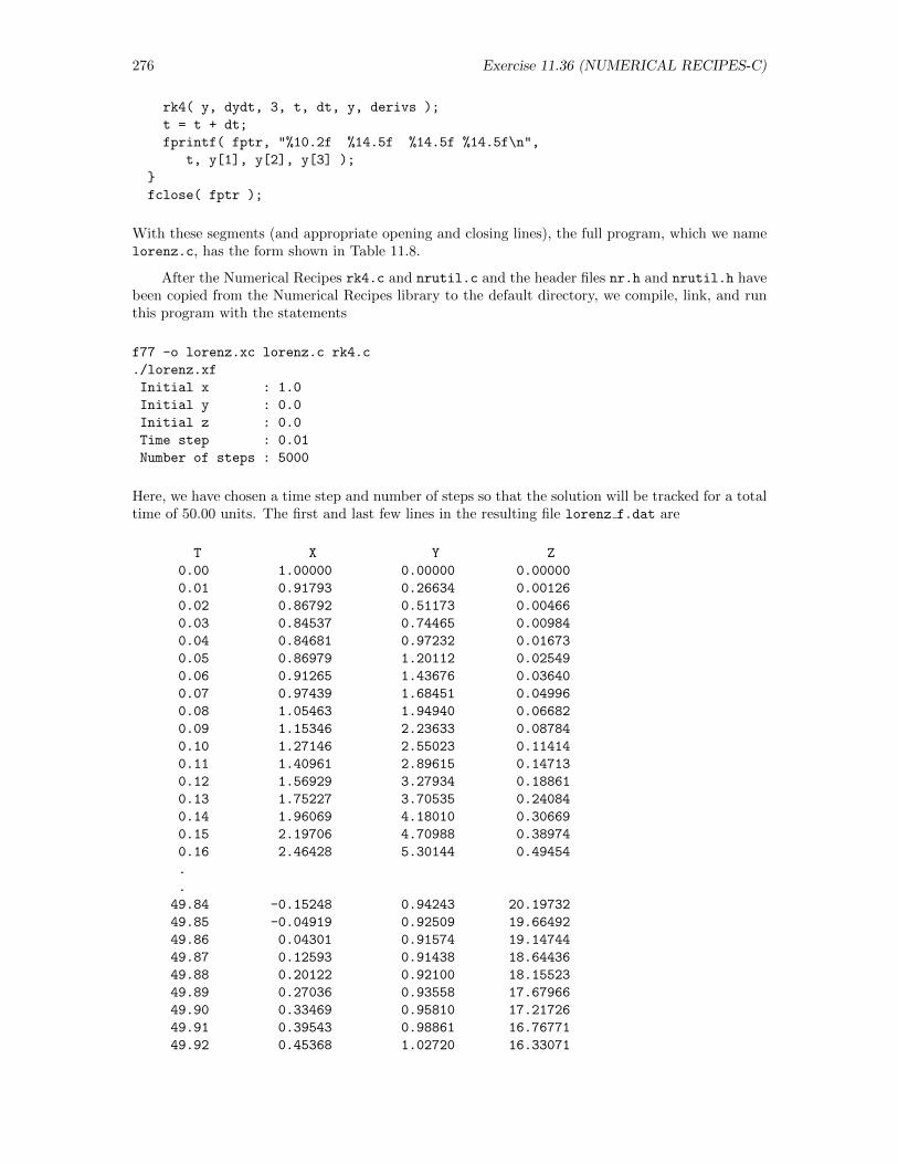
276 Exercise 11.36 (NUMERICAL RECIPES-C)
rk4( y, dydt, 3, t, dt, y, derivs );
t = t + dt;
fprintf( fptr, "%10.2f %14.5f %14.5f %14.5f\n",
t, y[1], y[2], y[3] );
fclose( fptr );
With these segments (and appropriate opening and closing lines), the full program, which we namelorenz.c, has the form shown in Table 11.8.
After the Numerical Recipes rk4.c and nrutil.c and the header files nr.h and nrutil.h havebeen copied from the Numerical Recipes library to the default directory, we compile, link, and runthis program with the statements
f77 -o lorenz.xc lorenz.c rk4.c
./lorenz.xf
Initial x : 1.0
Initial y : 0.0
Initial z : 0.0
Time step : 0.01
Number of steps : 5000
Here, we have chosen a time step and number of steps so that the solution will be tracked for a totaltime of 50.00 units. The first and last few lines in the resulting file lorenz f.dat are
T X Y Z
0.00 1.00000 0.00000 0.00000
0.01 0.91793 0.26634 0.00126
0.02 0.86792 0.51173 0.00466
0.03 0.84537 0.74465 0.00984
0.04 0.84681 0.97232 0.01673
0.05 0.86979 1.20112 0.02549
0.06 0.91265 1.43676 0.03640
0.07 0.97439 1.68451 0.04996
0.08 1.05463 1.94940 0.06682
0.09 1.15346 2.23633 0.08784
0.10 1.27146 2.55023 0.11414
0.11 1.40961 2.89615 0.14713
0.12 1.56929 3.27934 0.18861
0.13 1.75227 3.70535 0.24084
0.14 1.96069 4.18010 0.30669
0.15 2.19706 4.70988 0.38974
0.16 2.46428 5.30144 0.49454
.
.
49.84 -0.15248 0.94243 20.19732
49.85 -0.04919 0.92509 19.66492
49.86 0.04301 0.91574 19.14744
49.87 0.12593 0.91438 18.64436
49.88 0.20122 0.92100 18.15523
49.89 0.27036 0.93558 17.67966
49.90 0.33469 0.95810 17.21726
49.91 0.39543 0.98861 16.76771
49.92 0.45368 1.02720 16.33071
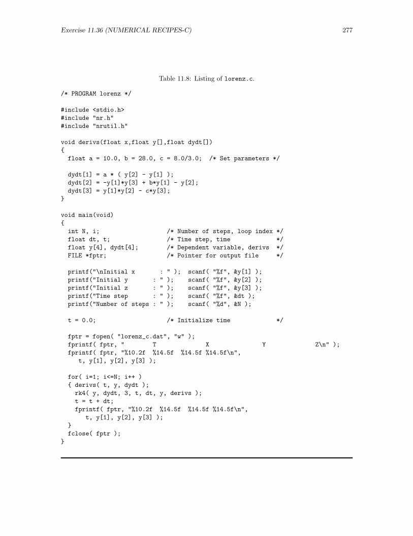
Exercise 11.36 (NUMERICAL RECIPES-C) 277
Table 11.8: Listing of lorenz.c.
/* PROGRAM lorenz */
#include <stdio.h>
#include "nr.h"
#include "nrutil.h"
void derivs(float x,float y[],float dydt[])
float a = 10.0, b = 28.0, c = 8.0/3.0; /* Set parameters */
dydt[1] = a * ( y[2] - y[1] );
dydt[2] = -y[1]*y[3] + b*y[1] - y[2];
dydt[3] = y[1]*y[2] - c*y[3];
void main(void)
int N, i; /* Number of steps, loop index */
float dt, t; /* Time step, time */
float y[4], dydt[4]; /* Dependent variable, derivs */
FILE *fptr; /* Pointer for output file */
printf("\nInitial x : " ); scanf( "%f", &y[1] );
printf("Initial y : " ); scanf( "%f", &y[2] );
printf("Initial z : " ); scanf( "%f", &y[3] );
printf("Time step : " ); scanf( "%f", &dt );
printf("Number of steps : " ); scanf( "%d", &N );
t = 0.0; /* Initialize time */
fptr = fopen( "lorenz_c.dat", "w" );
fprintf( fptr, " T X Y Z\n" );
fprintf( fptr, "%10.2f %14.5f %14.5f %14.5f\n",
t, y[1], y[2], y[3] );
for( i=1; i<=N; i++ )
derivs( t, y, dydt );
rk4( y, dydt, 3, t, dt, y, derivs );
t = t + dt;
fprintf( fptr, "%10.2f %14.5f %14.5f %14.5f\n",
t, y[1], y[2], y[3] );
fclose( fptr );
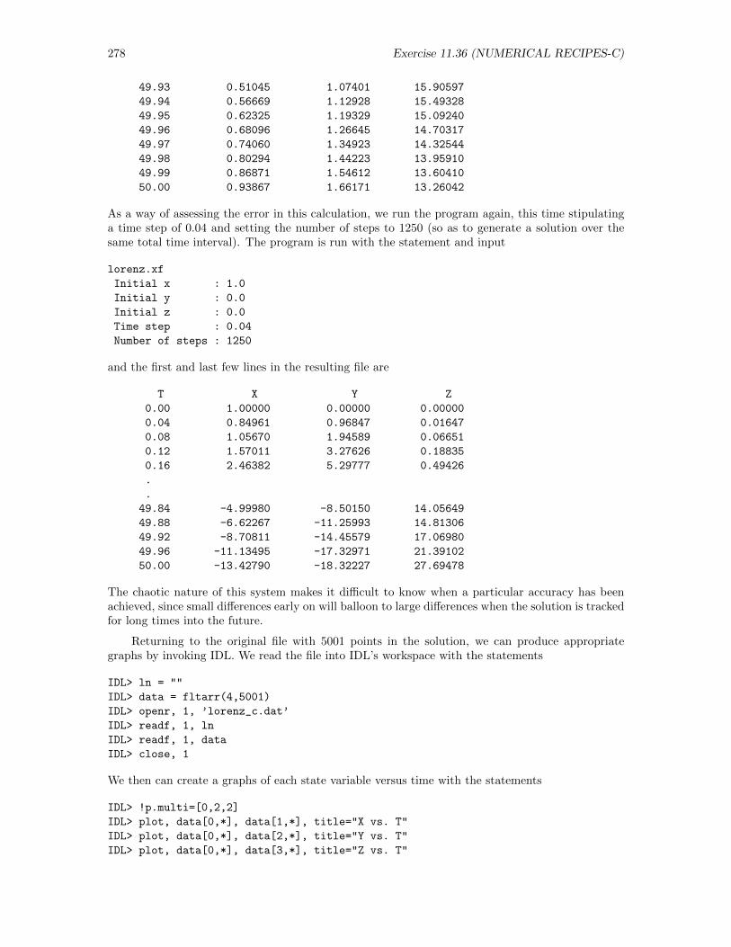
278 Exercise 11.36 (NUMERICAL RECIPES-C)
49.93 0.51045 1.07401 15.90597
49.94 0.56669 1.12928 15.49328
49.95 0.62325 1.19329 15.09240
49.96 0.68096 1.26645 14.70317
49.97 0.74060 1.34923 14.32544
49.98 0.80294 1.44223 13.95910
49.99 0.86871 1.54612 13.60410
50.00 0.93867 1.66171 13.26042
As a way of assessing the error in this calculation, we run the program again, this time stipulatinga time step of 0.04 and setting the number of steps to 1250 (so as to generate a solution over thesame total time interval). The program is run with the statement and input
lorenz.xf
Initial x : 1.0
Initial y : 0.0
Initial z : 0.0
Time step : 0.04
Number of steps : 1250
and the first and last few lines in the resulting file are
T X Y Z
0.00 1.00000 0.00000 0.00000
0.04 0.84961 0.96847 0.01647
0.08 1.05670 1.94589 0.06651
0.12 1.57011 3.27626 0.18835
0.16 2.46382 5.29777 0.49426
.
.
49.84 -4.99980 -8.50150 14.05649
49.88 -6.62267 -11.25993 14.81306
49.92 -8.70811 -14.45579 17.06980
49.96 -11.13495 -17.32971 21.39102
50.00 -13.42790 -18.32227 27.69478
The chaotic nature of this system makes it difficult to know when a particular accuracy has beenachieved, since small differences early on will balloon to large differences when the solution is trackedfor long times into the future.
Returning to the original file with 5001 points in the solution, we can produce appropriategraphs by invoking IDL. We read the file into IDL’s workspace with the statements
IDL> ln = ""
IDL> data = fltarr(4,5001)
IDL> openr, 1, ’lorenz_c.dat’
IDL> readf, 1, ln
IDL> readf, 1, data
IDL> close, 1
We then can create a graphs of each state variable versus time with the statements
IDL> !p.multi=[0,2,2]
IDL> plot, data[0,*], data[1,*], title="X vs. T"
IDL> plot, data[0,*], data[2,*], title="Y vs. T"
IDL> plot, data[0,*], data[3,*], title="Z vs. T"
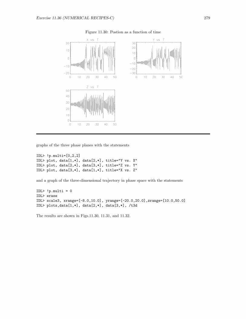
Exercise 11.36 (NUMERICAL RECIPES-C) 279
Figure 11.30: Postion as a function of time
graphs of the three phase planes with the statements
IDL> !p.multi=[0,2,2]
IDL> plot, data[1,*], data[2,*], title="Y vs. X"
IDL> plot, data[2,*], data[3,*], title="Z vs. Y"
IDL> plot, data[3,*], data[1,*], title="X vs. Z"
and a graph of the three-dimensional trajectory in phase space with the statements
IDL> !p.multi = 0
IDL> erase
IDL> scale3, xrange=[-8.0,10.0], yrange=[-20.0,20.0],zrange=[10.0,50.0]
IDL> plots,data[1,*], data[2,*], data[3,*], /t3d
The results are shown in Figs.11.30, 11.31, and 11.32.
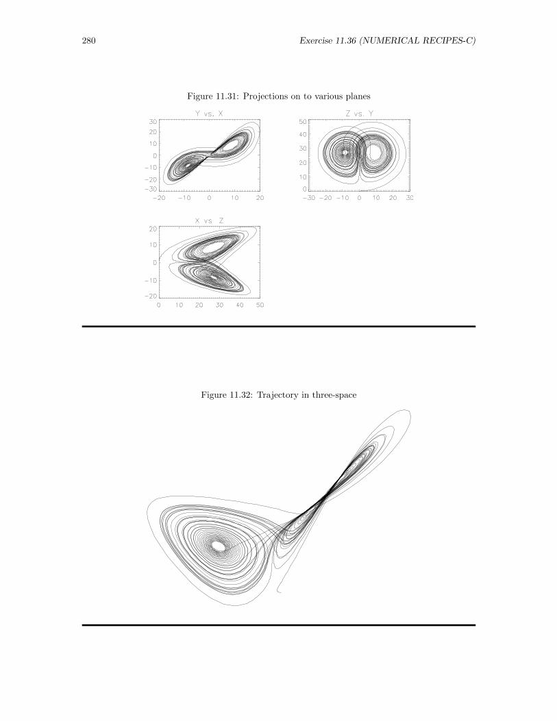
280 Exercise 11.36 (NUMERICAL RECIPES-C)
Figure 11.31: Projections on to various planes
Figure 11.32: Trajectory in three-space
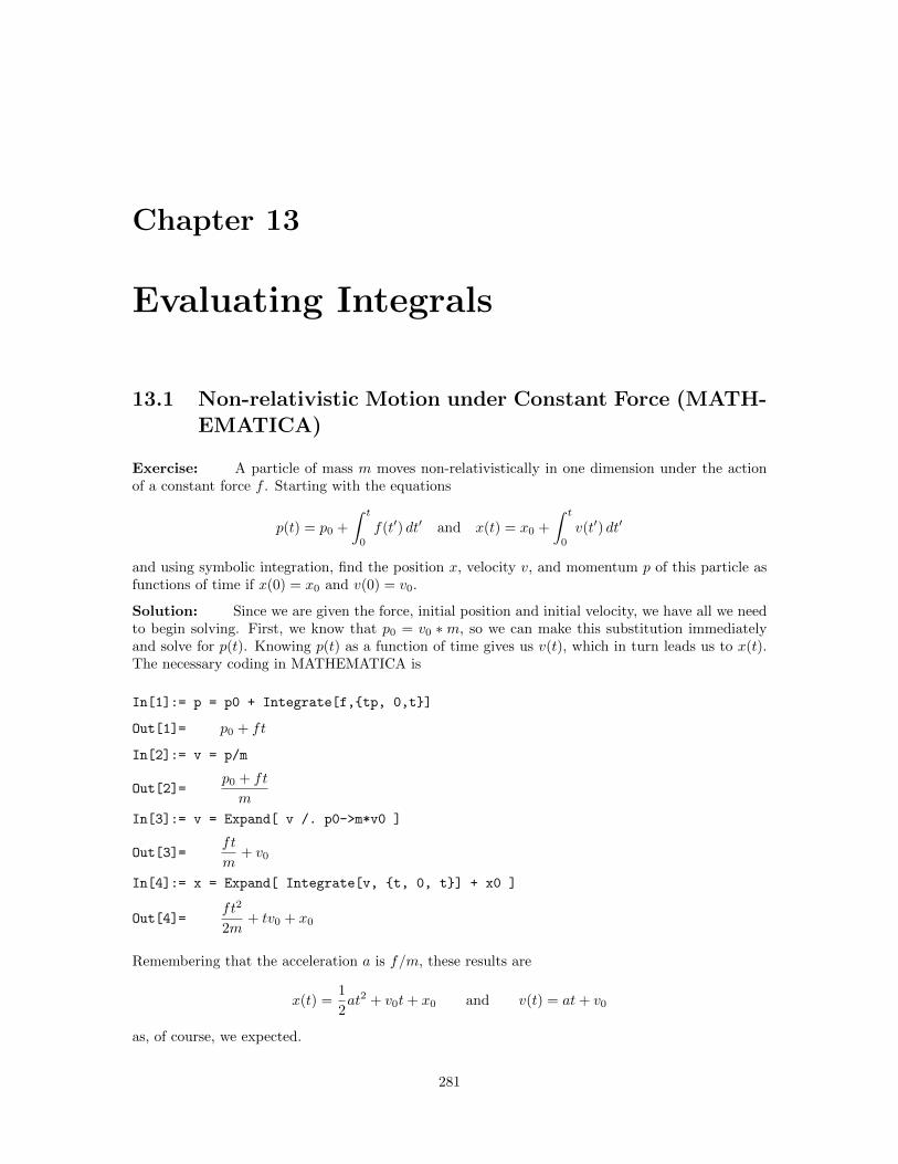
Chapter 13
Evaluating Integrals
13.1 Non-relativistic Motion under Constant Force (MATH-EMATICA)
Exercise: A particle of mass m moves non-relativistically in one dimension under the actionof a constant force f . Starting with the equations
p(t) = p0 +
∫ t
0
f(t′) dt′ and x(t) = x0 +
∫ t
0
v(t′) dt′
and using symbolic integration, find the position x, velocity v, and momentum p of this particle asfunctions of time if x(0) = x0 and v(0) = v0.
Solution: Since we are given the force, initial position and initial velocity, we have all we needto begin solving. First, we know that p0 = v0 ∗m, so we can make this substitution immediatelyand solve for p(t). Knowing p(t) as a function of time gives us v(t), which in turn leads us to x(t).The necessary coding in MATHEMATICA is
In[1]:= p = p0 + Integrate[f,tp, 0,t]
Out[1]= p0 + ft
In[2]:= v = p/m
Out[2]=p0 + ft
m
In[3]:= v = Expand[ v /. p0->m*v0 ]
Out[3]=ft
m+ v0
In[4]:= x = Expand[ Integrate[v, t, 0, t] + x0 ]
Out[4]=ft2
2m+ tv0 + x0
Remembering that the acceleration a is f/m, these results are
x(t) =1
2at2 + v0t+ x0 and v(t) = at+ v0
as, of course, we expected.
281
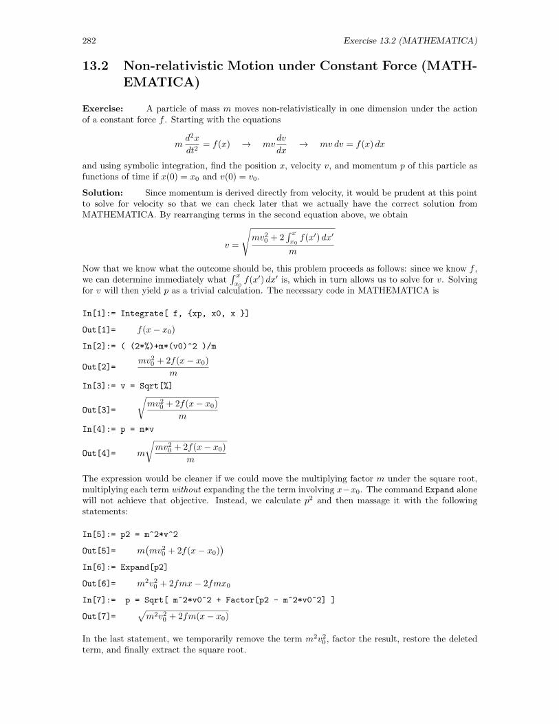
282 Exercise 13.2 (MATHEMATICA)
13.2 Non-relativistic Motion under Constant Force (MATH-EMATICA)
Exercise: A particle of mass m moves non-relativistically in one dimension under the actionof a constant force f . Starting with the equations
md2x
dt2= f(x) → mv
dv
dx→ mv dv = f(x) dx
and using symbolic integration, find the position x, velocity v, and momentum p of this particle asfunctions of time if x(0) = x0 and v(0) = v0.
Solution: Since momentum is derived directly from velocity, it would be prudent at this pointto solve for velocity so that we can check later that we actually have the correct solution fromMATHEMATICA. By rearranging terms in the second equation above, we obtain
v =
√mv2
0 + 2∫ xx0f(x′) dx′
m
Now that we know what the outcome should be, this problem proceeds as follows: since we know f ,we can determine immediately what
∫ xx0f(x′) dx′ is, which in turn allows us to solve for v. Solving
for v will then yield p as a trivial calculation. The necessary code in MATHEMATICA is
In[1]:= Integrate[ f, xp, x0, x ]
Out[1]= f(x− x0)
In[2]:= ( (2*%)+m*(v0)^2 )/m
Out[2]=mv2
0 + 2f(x− x0)
m
In[3]:= v = Sqrt[%]
Out[3]=
√mv2
0 + 2f(x− x0)
m
In[4]:= p = m*v
Out[4]= m
√mv2
0 + 2f(x− x0)
m
The expression would be cleaner if we could move the multiplying factor m under the square root,multiplying each term without expanding the the term involving x−x0. The command Expand alonewill not achieve that objective. Instead, we calculate p2 and then massage it with the followingstatements:
In[5]:= p2 = m^2*v^2
Out[5]= m(mv2
0 + 2f(x− x0))
In[6]:= Expand[p2]
Out[6]= m2v20 + 2fmx− 2fmx0
In[7]:= p = Sqrt[ m^2*v0^2 + Factor[p2 - m^2*v0^2] ]
Out[7]=√m2v2
0 + 2fm(x− x0)
In the last statement, we temporarily remove the term m2v20 , factor the result, restore the deleted
term, and finally extract the square root.
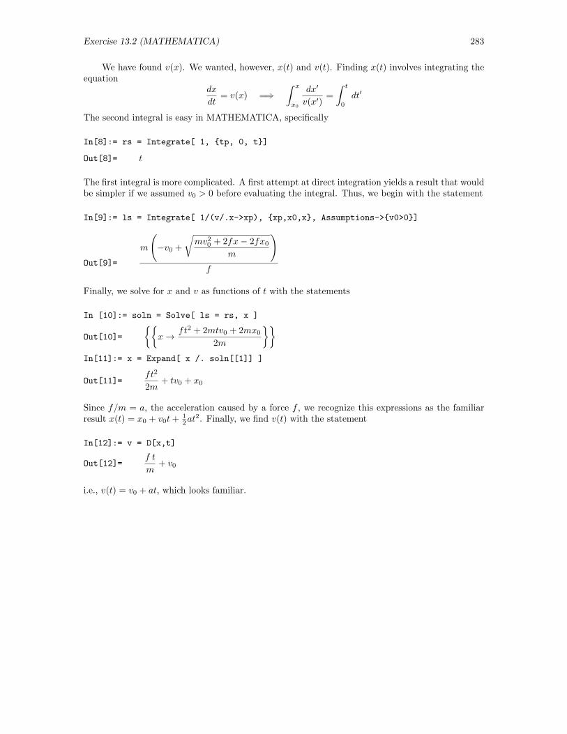
Exercise 13.2 (MATHEMATICA) 283
We have found v(x). We wanted, however, x(t) and v(t). Finding x(t) involves integrating theequation
dx
dt= v(x) =⇒
∫ x
x0
dx′
v(x′)=
∫ t
0
dt′
The second integral is easy in MATHEMATICA, specifically
In[8]:= rs = Integrate[ 1, tp, 0, t]
Out[8]= t
The first integral is more complicated. A first attempt at direct integration yields a result that wouldbe simpler if we assumed v0 > 0 before evaluating the integral. Thus, we begin with the statement
In[9]:= ls = Integrate[ 1/(v/.x->xp), xp,x0,x, Assumptions->v0>0]
Out[9]=
m
(−v0 +
√mv2
0 + 2fx− 2fx0
m
)f
Finally, we solve for x and v as functions of t with the statements
In [10]:= soln = Solve[ ls = rs, x ]
Out[10]=
x→ ft2 + 2mtv0 + 2mx0
2m
In[11]:= x = Expand[ x /. soln[[1]] ]
Out[11]=ft2
2m+ tv0 + x0
Since f/m = a, the acceleration caused by a force f , we recognize this expressions as the familiarresult x(t) = x0 + v0t+ 1
2at2. Finally, we find v(t) with the statement
In[12]:= v = D[x,t]
Out[12]=f t
m+ v0
i.e., v(t) = v0 + at, which looks familiar.
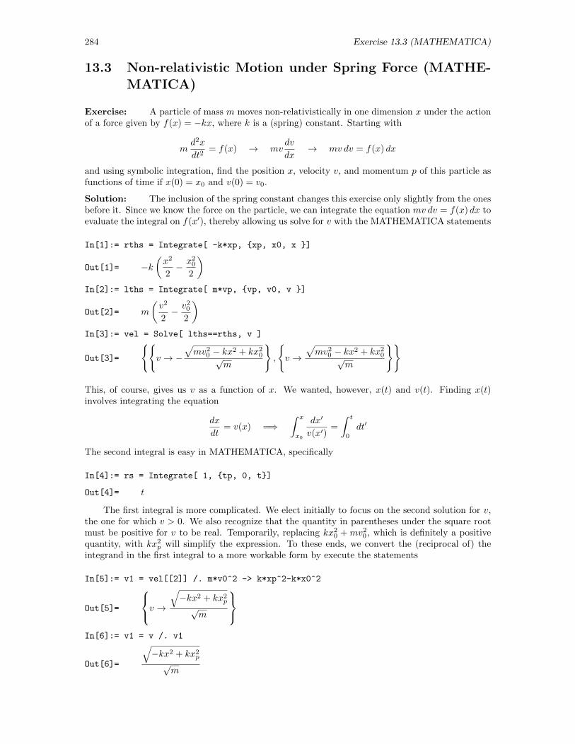
284 Exercise 13.3 (MATHEMATICA)
13.3 Non-relativistic Motion under Spring Force (MATHE-MATICA)
Exercise: A particle of mass m moves non-relativistically in one dimension x under the actionof a force given by f(x) = −kx, where k is a (spring) constant. Starting with
md2x
dt2= f(x) → mv
dv
dx→ mv dv = f(x) dx
and using symbolic integration, find the position x, velocity v, and momentum p of this particle asfunctions of time if x(0) = x0 and v(0) = v0.
Solution: The inclusion of the spring constant changes this exercise only slightly from the onesbefore it. Since we know the force on the particle, we can integrate the equation mv dv = f(x) dx toevaluate the integral on f(x′), thereby allowing us solve for v with the MATHEMATICA statements
In[1]:= rths = Integrate[ -k*xp, xp, x0, x ]
Out[1]= −k(x2
2− x2
0
2
)In[2]:= lths = Integrate[ m*vp, vp, v0, v ]
Out[2]= m
(v2
2− v2
0
2
)In[3]:= vel = Solve[ lths==rths, v ]
Out[3]=
v → −
√mv2
0 − kx2 + kx20√
m
,
v →
√mv2
0 − kx2 + kx20√
m
This, of course, gives us v as a function of x. We wanted, however, x(t) and v(t). Finding x(t)involves integrating the equation
dx
dt= v(x) =⇒
∫ x
x0
dx′
v(x′)=
∫ t
0
dt′
The second integral is easy in MATHEMATICA, specifically
In[4]:= rs = Integrate[ 1, tp, 0, t]
Out[4]= t
The first integral is more complicated. We elect initially to focus on the second solution for v,the one for which v > 0. We also recognize that the quantity in parentheses under the square rootmust be positive for v to be real. Temporarily, replacing kx2
0 + mv20 , which is definitely a positive
quantity, with kx2p will simplify the expression. To these ends, we convert the (reciprocal of) the
integrand in the first integral to a more workable form by execute the statements
In[5]:= v1 = vel[[2]] /. m*v0^2 -> k*xp^2-k*x0^2
Out[5]=
v →√−kx2 + kx2
p√m
In[6]:= v1 = v /. v1
Out[6]=
√−kx2 + kx2
p√m
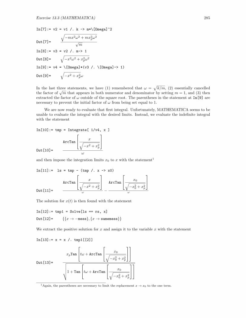
Exercise 13.3 (MATHEMATICA) 285
In[7]:= v2 = v1 /. k -> m*\[Omega]^2
Out[7]=
√−mx2ω2 +mx2
pω2
√m
In[8]:= v3 = v2 /. m-> 1
Out[8]=√−x2ω2 + x2
pω2
In[9]:= v4 = \[Omega]*(v3 /. \[Omega]-> 1)
Out[9]=√−x2 + x2
pω
In the last three statements, we have (1) remembered that ω =√k/m, (2) essentially cancelled
the factor of√m that appears in both numerator and denominator by setting m = 1, and (3) then
extracted the factor of ω outside of the square root. The parentheses in the statement at In[9] arenecessary to prevent the initial factor of ω from being set equal to 1.
We are now ready to evaluate that first integral. Unfortunately, MATHEMATICA seems to beunable to evaluate the integral with the desired limits. Instead, we evaluate the indefinite integralwith the statement
In[10]:= tmp = Integrate[ 1/v4, x ]
Out[10]=
ArcTan
x√−x2 + x2
p
ω
and then impose the integration limits x0 to x with the statement1
In[11]:= ls = tmp - (tmp /. x -> x0)
Out[11]=
ArcTan
x√−x2 + x2
p
ω −
ArcTan
x0√−x2
0 + x2p
ω
The solution for x(t) is then found with the statement
In[12]:= tmp1 = Solve[ls == rs, x]
Out[12]= x→ −mess, x→ samemess
We extract the positive solution for x and assign it to the variable x with the statement
In[13]:= x = x /. tmp1[[2]]
Out[13]=
xpTan
tω + ArcTan
x0√−x2
0 + x2p
√√√√√1 + Tan
tω + ArcTan
x0√−x2
0 + x2p
1Again, the parentheses are necessary to limit the replacement x→ x0 to the one term.
286 Exercise 13.3 (MATHEMATICA)
Recognizing that the arctangent in this result is a constant and simply a phase, we simplify the entireexpression by replacing that complicated expression with a single symbol φ with the statement
In[14]:= x1 = x /. ArcTan[x0/Sqrt[-x0^2+xp^2]] -> \[Phi]
Out[14]=xpTan[φ+ tω]√1 + Tan[φ+ tω]2
and then simplify the expression further with the statements
In[15]:= x2 = Simplify[ x1, trig ]
Out[15]=xpTan[φ+ tω]√Sec[φ+ tω]2
In[16]:= x = Assuming[ Sec[\[Phi]+t*\[Omega]]>0, Refine[x2]]
Out[16]= xp Sin[φ+ tω]
From here, we find the velocity and momentum as functions of time with the statements
In[17]:= v = D[x,t]
Out[17]= xpωCos[φ+ tω]
In[17]:= p = m*v
mxpωCos[φ+ tω]
Strictly, this solution applies only when v > 0. Fortuitously, however, it happens to apply alsowhen v < 0, as repeating the above steps with the second solution for v will reveal. Remember thatω =
√k/m and
k ∗ x2p = m ∗ v2
0 + k ∗ x20 =⇒ x2
p = x20 +
mv20
k= x2
0 +v2
0
ω2
and
φ = ArcTan
x0√x2p − x2
0
= ArcTan
(ωx0
v0
)
Exercise 13.4 (Mathematica) 287
13.4 Non-Relativistic Motion with Decaying Force (Mathe-matica)
Exercise: Suppose an object of mass m moves non-relativistically in one dimension under theaction of the force f(t) = f0e
−bt, where both b and f0 are positive. Let x(0) = x0 and v(0) = v0.Use symbolic integration to find x(t) and v(t) by evaluating the integrals in the equations
p(t) = p0 +
∫ t
0
f(t′) dt′ and x(t) = x0 +
∫ t
0
v(t′) dt′
Then, find and interpret both the limits of these two results as t→∞ and the Taylor expansion ofthese two results for small t.
Solution: When the force experienced by a particle moving non-relativistically is given by
f(t) = f0e−bt
the dynamic problem to be solved to find the motion is conveyed by the equations
md2x
dt2= f0e
−bt ; x(0) = x0 ; v(0) = v0
where v(t) = dx(t)/dt. To find this solution by direct integration, we begin by recognizing fromEq. (11.3) that
p(t) = mv(t) = mv0 +
∫ t
0
f(t′) dt′ = mv0 +
∫ t
0
f0 e−bt′ dt′
and we evaluate this integral in Mathematica with the statements
In[1]:= f = f0*Exp[-b*tp];
In[2]:= p = m*v0 + Integrate[ f, tp, 0, t ]
Out[2]=
(1
b− e−bt
b
)f0 +mv0
Then, remembering that
x(t) = x0 +
∫ t
0
v(t′) dt′
and that, non-relativistically, p(t) = mv(t) and mindful also of the need to keep integration variablesseparate from the limits of integration, we determine the velocity and integrate the result one moretime with the statements
In[3]:= v = Simplify[p/m]
Out[3]=f0− e−btf0 + bmv0
bm
In[4]:= vp = v /. t -> tp;
In[5]:= x = Simplify[ x0 + Integrate[ vp, tp, 0, t ] ]
Out[5]= −(f0 − e−btf0
b2m
)+f0t
bm+ tv0 + x0
In[6]:= x = Collect[ Collect[x, t], 1/(b^2*m) ]
Out[6]=−f0 + e−btf0
b2m+ t
(f0
bm+ v0
)+ x0
288 Exercise 13.4 (Mathematica)
At present, Mathematica’s Limit function does not have the capacity to accept assumptionsabout the variables appearing in its first argument. The simple evaluation of the limits of v and xas t→∞ is therefore not possible; Mathematica returns an unevaluated form of the limit. We can,however, substitute a new variable, say T , for bt in the expressions and then evaluate the limits. Forthe velocity, we could use the statements
In[7]:= vv = v /. t -> T/b
Out[7]=f0 − e−T f0 + bmv0
bm
In[8]:= Limit[ vv, T -> Infinity ]
Out[8]=f0
bm+ v0
(Technically, we should restore the original variable t, but the result does not depend on T , so sucha replacement would have no effect on the result.) For the position, we would start with the similarstatement
In[9]:= xx = x /. t -> T/b
Out[9]= −f0 + e−T f0
b2m+T (f0/(bm) + v0)
b+ x0
Unfortunately, the simple statement Limit[ %, T -> Infinity ] returns an unevaluated form.Further, invoking Map to apply the function Limit to each term separately does not seem to work.The statement
In[10]:= Limit[ xx[[1]], T -> Infinity ] + Limit[ xx[[2]], T -> Infinity ]
+ Limit[ xx[[3]], T -> Infinity ]
Out[10]= − f0
b2m+ x0 +
(f0 + bmv0)∞b2m
does yield a useful result. We find that the velocity approaches a constant limiting value whilethe position increases in magnitude indefinitely, becoming large and positive or large and negative(depending on the algebraic sign of f0 + bmv0, i.e., on the relationship between the initial force andthe initial velocity). In the special case that v0 = −f0/bm, the terminal velocity is zero and, lookingagain at the expression for x, we conclude that the object comes ultimately to rest at the positionx = x0 − f0/b
2m.
To evaluate the limit as t becomes small, we choose to evaluate a Taylor series rather than lookspecifically to the limit. We invoke the statements
In[11]:= Series[ x, t, 0, 3 ]
Out[11]= x0 + v0t+f0t
2
2m− bf0t
3
6m+O(t)
4
In[12]:= Series[ v, t, 0, 2 ]
Out[12]= v0 +f0t
m− bf0t
2
2m+O(t)
3
We find that the first few terms in these expansions coincide with what we would expect for aconstant force f0 but then, as t becomes a bit larger (and the force becomes smaller), the positionand the velocity depart from those appropriate to constant force. Not surprisingly, for a short whilethis motion looks like motion under a constant force.
Exercise 13.5 (Mathematica) 289
13.5 Properties of Lorentz Distribution (Mathematica)
Exercise: The normalized Lorentz distribution function is given by
p(x) =1
π
a/2
x2 + (a/2)2
Using symbolic integration, (a) verify that∫ +∞−∞ p(x) dx = 1, (b) evaluate—as best you can—the
average x and variance σ2, defined by
x = limb→∞
∫ +b
−bx p(x) dx and σ2 = lim
b→∞
∫ +b
−b(x− x)2 p(x) dx
for this distribution, and (c) find the probability that a single, randomly selected value will lie inthe range −a ≤ x ≤ a. Finally, (d) show analytically that you should have expected the result ofpart (c) to be independent of a. Hint : Introduce the dimensionless variable λ = x/a.
Solution: The normalized Lorentz distribution function is
p(x) =1
π
a/2
x2 + (a/2)2
(a) Using symbolic integration, we can show that∫∞−∞ p(x) dx = 1 by setting up the integrand in
Mathematica and evaluating the integral with the limits −∞ to +∞. We use the statements
In[1]:= integrand = (1/\[Pi])*(a/2)/(x^2 + (a/2)^2);
In[2]:= Integrate[ integrand, x, -Infinity, Infinity, Assumptions -> a > 0 ]
Out[2]= 1
(b) The average x and the variance σ2 are defined by
x = limb→∞
∫ +b
−bx p(x) dx and σ2 = lim
b→∞
∫ +b
−b(x− x)2p(x) dx
respectively. To find x, we evaluate the integral on the symmetric finite interval −b ≤ x ≤ b andthen allow the limits to expand to infinity. We invoke the statements
In[3]:= Integrate[ integrand*x, x, -b, b, Assumptions -> b > 0 ]
Out[3]= 0
In[4]:= Limit[ %, b -> Infinity ]
Out[4]= 0
To evaluate σ2, we substitute the value for x and evaluate the integral defining σ2 with the statements
In[5]:= Integrate[ x^2 *integrand, x, -b, b, Assumptions -> b > 0 ];
In[6]:= Limit[ %, b -> Infinity ]
Out[6]= a∞
As we might have expected from the nature of the integrand in the integral giving σ2, the variancediverges for the Lorentz distribution. We note, even though Mathematica does not, that a∞ issimply ∞.
(c) To find the probability that a single, randomly selected value will be in the range −a ≤ x ≤ a,we need to evaluate the integral
∫ a−a p(x) dx. Since the integrand has already been defined earlier
in this exercise, we can continue our session with statements
290 Exercise 13.5 (Mathematica)
In[7]:= Integrate[integrand, x, -a, a, Assumptions -> a > 0];
In[8]:= ComplexExpand[%]
Out[8]= 2arctan(2)
π
In[9]:= N[%7]
Out[9]= 0.704833
(d) To show analytically that part (c) is independent of a, we introduce the dimensionless variableλ = x/a. Since dλ = dx/a, the new form of our equation is∫ a
−ap(x) dx =
1
2π
∫ 1
−1
1
λ2 + (1/4)dλ
Since all trace of a can be absorbed in this form, we know that the specific value of the integral isindependent of a.
Exercise 13.6 (Mathematica) 291
13.6 Earth Falling into Sun (Mathematica)
Exercise: Suppose some cataclysmic event stops the earth dead in its tracks and, respondingto the sun’s gravitational attraction, the earth falls into the sun. Using symbolic integration, findthe time required for the earth to fall over the middle half of its journey to the sun. Expressedin years, what is the value of this time for the earth-sun system? Hint : Since the gravitationalpotential is −GmM/x, conservation of energy yields
1
2m
(dx
dt
)2
−GmMx
= −GmMx0
=⇒ dx
dt= −√
2GM
√1
x− 1
x0
(The negative square root is taken because x, the distance to the sun, is known to be decreasing.)This expression then leads to the value
Tmidhalf =1√
2GM
∫ 3x0/4
x0/4
(1
x− 1
x0
)−1/2
dx
Hint : The evaluation will be simpler if you begin by recasting the problem in dimensionless terms,expressing lengths in units of x0 and times in units of
√x3
0/(2GM). To interpret the significanceof this unit of time, determine the period of a circular orbit of radius x0, which will turn out to be2π√x3
0/GM . For the earth around the sun, this latter time is, of course, 1 year. Optional : Evaluatethe time required for the first half of the journey, which involves a convergent but improper integral.
Solution: Should the earth stop, the time it would take for it to fall towards the sun over thecenter half of its path is given by the integral
Tmidhalf =1√
2GM
∫ 3x0/4
x0/4
(1
x− 1
x0
)−1/2
dx
To evaluate this integral symbolically in Mathematica, we set up the integrand and integrate. Recallthat the distances, although decreasing, are positive. We invoke the statements
In[1]:= integrand = (1/x - 1/x0)^(-1/2);
In[2]:= Integrate[integrand, x, x0/4, 3*x0/4];
In[3]:= ComplexExpand[%];
In[4]:= Simplify[%, x0 > 0]
Out[4]=1
6πx0
3/2
In[5]:= tmid = % / Sqrt[2*G*M]
Out[5]=πx0
3/2
6√
2√GM
Now, to find the period of a circular orbit at radius x0, we first require that the gravitational forcematch the required centripetal force, i.e., that
mv2
x0=GmM
x20
=⇒ v =
√GM
x0
and then compute the period from the relationship
T0 =2πx0
v=
2πx0√GM/x0
=2πx
3/20√
GM
To cast the above result as a multiple of T0, we execute the statements
292 Exercise 13.6 (Mathematica)
In[6]:= t0 = 2*Pi*x0^(3/2)/Sqrt[G*M]
Out[6]=2πx0
3/2
√GM
In[7]:= tmid/t0
Out[7]=1
12√
2
In[8]:= N[%]
Out[8]= 0.0589256
In[9]:= %*365
Out[9]= 21.5078
We find that the time required for the earth to fall towards the sun through the middle half of its
journey is given symbolically by πx3/20 /6
√2√GM and numerically by 0.0589 years or 21.51 days.
The time required for the first half of the journey can be found by changing the the upperlimit of integration to x0 and the lower limit to x0/2. To evaluate, we continue our session with thestatements
In[10]:= Integrate[integrand, x, x0/2, x0, Assumptions -> ( x0 > 0)]
Out[10]=1
4(2 + π) x0
3/2
In[11]:= tfirst = % / Sqrt[2*G*M]
Out[11]=(2 + π)x0
3/2
4√
2√GM
Again, casting in terms of the period of the circular orbit of radius x0, we find that this time is givenby
In[12]:= tfirst/t0
Out[12]=2 + π
8√
2π
In[13]:= N[%]
Out[13]= 0.144658
In[14]:= %*365
Out[14]= 52.8002
We find that the time required for the earth to fall towards the sun through the first half of its journey
is given symbolically by (2 + π)x3/20 /4
√2√GM and numerically by 0.1447 years or 52.80 days.
Finally, let us find the time required for the earth to fall all the way from its starting point tothe sun. We execute the statements
In[15]:= Integrate[integrand, x, 0, x0, Assumptions -> ( x0 > 0)]
Out[15]=1
2x
3/20
In[16]:= tfull = %/Sqrt[2*G*M]
Out[16]=πx
3/20
2√
2GM

Exercise 13.6 (Mathematica) 293
In[17]:= tfull/t0
Out[17]=1
4√
2
In[18]:= N[%]
Out[18]= 0.176777
In[19]:= %*365
Out[19]= 64.5235
From start to finish in this calamity requires a mere 64.5 days!
294 Exercise 13.7 (Mathematica)
13.7 Electron inside Bohr Radius (Mathematica)
Exercise: According to the quantum theory, the probability that the electron in the groundstate of the hydrogen atom will be found between the center of the atom and some radius r is givenby
P (r) =4
a3
∫ r
0
e−2r′/ar′2dr′ = 4
∫ r/a
0
e−2ρ ρ2 dρ
where a is the Bohr radius and ρ = r′/a. Evaluate this integral symbolically. Then plot and commenton a graph of P (r) versus r/a.
Solution: In this exercise, we are to examine the probability that an electron in the groundstate of the hydrogen atom will be found between the center of the atom and some radius r. Thisprobability is given by the equation
P (r) = 4
∫ r/a
0
e−2ρρ2 dρ
where a is the Bohr radius. To explore the probability in Mathematica as a function of r/a, we mustidentify the integrand and evaluate the integral. Introducing the dimensionless variable s = r/a, weexecute the statements
In[1]:= integrand = Exp[-2*\[Rho]]*\[Rho]^2;
In[2]:= p = 4 * Integrate[%, \[Rho], 0, s];
In[3]:= p = Simplify[%];
In[4]:= p = Collect[p, Exp[-2*s]]
Out[4]= 1 + e(−2s) (−1− 2s− 2s2)
In[5]:= Plot[p, s, 0.0, 4.0, PlotStyle -> AbsoluteThickness[3],
AxesLabel -> "r/a", "p"]
The first statement sets up the integrand and binds it to the variable integrand. The secondstatement evaluates the integral from 0 to s, and the third and fourth statements rearrange theresult into a somewhat more readable form. Then, using the last statement, in which we allow thevalues of s to range from 0.0 to 4.0, we plot p as a function of s. The resulting graph is shown inFig. 13.1. Note that the value of P (s) goes to 1 as s approaches infinity.
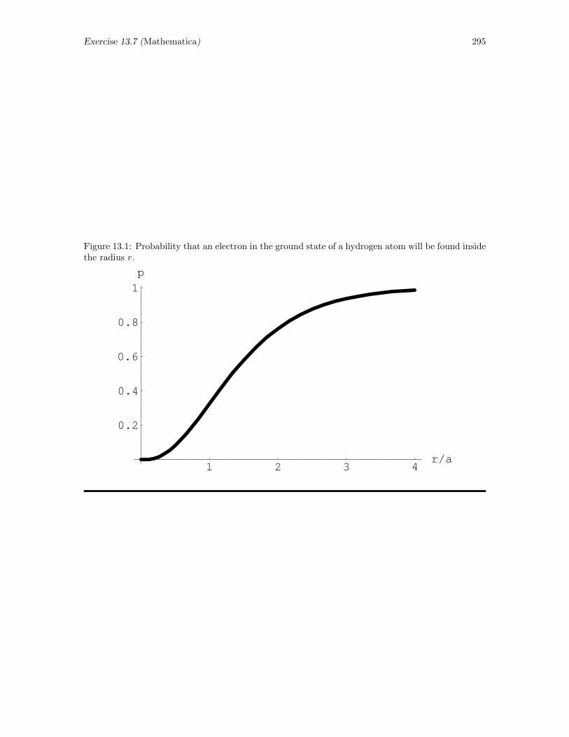
Exercise 13.7 (Mathematica) 295
Figure 13.1: Probability that an electron in the ground state of a hydrogen atom will be found insidethe radius r.
1 2 3 4r/a
0.2
0.4
0.6
0.8
1
p
296 Exercise 13.8 (Mathematica)
13.8 On-Axis Potential of a Pair of Disks (Mathematica)
Exercise: Consider a source consisting of two uniformly charged disks, each of radius a andeach oriented with its center on the z axis and its plane perpendicular to the z axis. Let one diskhave its center at (0,0,ca) and carry a positive charge density σ and the other have its center at(0,0,−ca) and carry a negative charge density −σ. Using a symbolic program, show that the on-axiselectrostatic potential established by this source is given by
V (z) =σ
2ε0
[√a2 + (z − ca)2 − |z − ca| −
√a2 + (z + ca)2 + |z + ca|
]and then explore this potential as a function of z/a for various values of c. Hint : First find theon-axis potential of a single disk lying in the xy plane, and then construct the desired potential bysuperposition.
Solution: Consider first the on-axis electrostatic potential of a single charged disk of radiusa located in the xy plane with its center at the origin. Then, the vectors r and r′ locating theobservation point on the z axis and an element of the source whose polar coordinates in the xyplane are (r′, φ′) are
r = z k ; r′ = r′ cosφ′ i + r′ sinφ′ j
and an element of the source subtending the angle dφ′ from the center of the circle has arear′ dφ′ dr′ and, with uniform charge density σ, carries charge dq′ = σr′ dφ′ dr′. Further, accord-ing to Eq. (11.28), the electrostatic potential at this observation point is given by
V (z) =σ
4πε0
∫ 2π
0
∫ a
0
r′ dr′ dφ′
|r− r′|
We need first to determine the integrand and then do the double integral. We invoke the Mathematicastatements2
In[1]:= ro = 0, 0, z ;
In[2]:= rp = r*Cos[\[Phi]],r*Sin[\[Phi]],0;
In[3]:= sep = ro + rp;
In[4]:= sep.sep;
In[5]:= Simplify[%];
In[6]:= den = Sqrt[%]
Out[6]=√r2 + z2
In[7]:= cnst = 1/(4*Pi*\[Epsilon][0]);
In[8]:= integ = \[Sigma]*cnst*r/den
Out[8]=rσ
4π√r2 + z2 ε0
In[9]:= Integrate[integ, r, 0, a]
In[10]:= single = Integrate[ %,
\[Phi],0,2*Pi ]
Out[10]=
(−√z2 +
√a2 + z2
)σ
2ε0
Set observation point.Set source point.Evaluate r− r′.Evaluate |r− r′|2.Recognize cos2 φ+ sin2 φ = 1Calculate denominator in integral.
Set constant.Evaluate integrand.
Evaluate integrals, doing the radial integralfirst.
Now, we are ready to construct from this potential the potential produced by a pair of identicaldisks, one carrying charge density σ and located at z = ca and the other carrying charge density−σ and located at z = −ca. We need simply recognize that the symbol z in the above evaluationrepresents the coordinate of the observation point relative to the center of the disk. Thus, we canconstruct the potential established by the pair of disks located as described from that of the single
2In this coding, we use r and phi for r′ and φ′.
Exercise 13.8 (Mathematica) 297
disk we have calculated simply by combining two pieces, for the first of which we replace z in theabove evaluation with z − ca and for the second of which we replace z with z + ca and σ with −σ.Equivalently, we subtract the above expression with z + ca replacing z from the above expressionwith z − ca replacing z. The appropriate Mathematica statements are
In[11]:= part1 = single /. z -> z - c*a;
In[12]:= part2 = single /. z -> z + c*a;
In[13]:= double = Collect[ part1 - part2, \[Sigma] ]
Out[13]:= σ
−√
(−ac+ z)2
+
√a2 + (−ac+ z)
2
2ε0+
√(ac+ z)
2 −√a2 + (ac+ z)
2
2ε0
Recognizing that
√q2 = |q|, we conclude that this result agrees with the result given in the exercise.
To explore this result for various values of c, it is wise to cast it in a dimensionless form byintroducing the coordinate zd = z/a and measuring the potential in units of σa/2ε0. Thus, wewant ultimately to replace z in the above expression with azd and divide the result by σa/2ε0.Unfortunately, we need to pursue these objectives in several steps. First, we substitute azd for z,then, in pieces, we remove the factors of σ, 2, and ε0 with the statements
In[14]:= Simplify[ 2*(double /. z -> a*zd)/\[Sigma] ];
In[15]:= Collect[%, \[Epsilon][0]];
In[16]:= tmp = %*\[Epsilon][0]
Out[16]=
√a2 (c+ zd)
2 −√
(a c− a zd)2 −√a2(
1 + (c+ zd)2)
+
√a2 + (a c− a zd)2
Clearly, there is now a common factor of a in every term. To complete the translation of thisexpression to a dimensionless form, we need to divide this result by a, thereby removing a from theexpression altogether. Simple setting a = 1 achieves the same end result. Rather than wrestle withpersuading Mathematica to factor the a out of these square roots, we elect the easier route with thestatement
In[17]:= pot = tmp /. a -> 1
Out[17]=
√1 + (c− zd)2 −
√(c− zd)2
+
√(c+ zd)
2 −√
1 + (c+ zd)2
At long last, we can plot this potential as a function of zd for various values of c. We invokethe statements
In[18]:= pot01 = pot /. c -> 0.1;
In[19]:= pot05 = pot /. c -> 0.5;
In[20]:= pot10 = pot /. c -> 1.0;
In[21]:= pot20 = pot /. c -> 2.0
In[22]:= graph = Plot[ pot01, pot05, pot10, pot20, zd, -4.0, 4.0,
PlotRange -> -1.0, 1.0, AxesLabel -> "z/a", "pot" ]
In[23]:= Display["integ-ex08-mathem-fig1.eps", graph, "EPS"]
The resulting graph is shown in Fig. 13.2. Note that, for the smaller values of c (at which theseparation of the disks is small compared to their common radius), the potential varies linearly aswe walk from one disk to the other in the region between them. As their separation grows relativeto their radius, that linearity is gradually destroyed. In all cases, however, the potential remainszero at the on-axis point midway between the two disks.
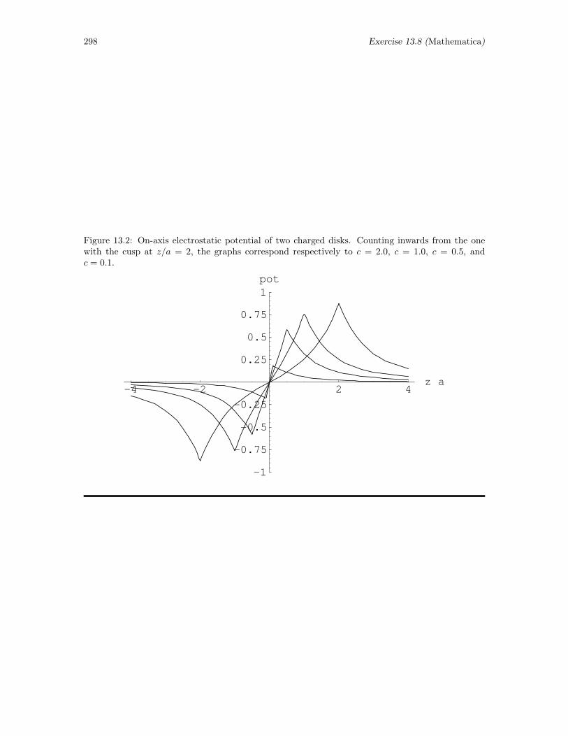
298 Exercise 13.8 (Mathematica)
Figure 13.2: On-axis electrostatic potential of two charged disks. Counting inwards from the onewith the cusp at z/a = 2, the graphs correspond respectively to c = 2.0, c = 1.0, c = 0.5, andc = 0.1.
-4 -2 2 4za
-1
-0.75
-0.5
-0.25
0.25
0.5
0.75
1pot
Exercise 13.10 (Mathematica) 299
13.10 Properties of Cardioid (Mathematica)
Exercise: Consider a surface in the xy plane having uniform mass density σ and having theshape of a cardioid given in polar coordinates by the function r(φ) = a(1 − cosφ). Using symbolicintegration, find (a) the center of mass of this object, (b) the moment of inertia tensor of this objectabout the x, y, and z axes, and (c) the radius of gyration about the z axis. Hints: The center ofmass is defined in Section 13.1.2; the moment of inertia tensor is a 3× 3 tensor whose ij element isgiven by
Iij =
∫[(x2
1 + x22 + x2
3)δij − xixj ] dm
where x1, x2, and x3 symbolize x, y, and z, respectively; δij is the Kronecker delta, which has thevalue 1 when i = j and the value 0 otherwise; and the radius of gyration is defined in Section 13.1.3.
Solution: (a) The location of the center of mass of an object is given by the equation
rcm =1
M
∫r dm =
1
M
∫σ(r, φ) r r dr dφ
In this case, σ is a constant. We can write r = r cosφ i + r sinφ j and then perform the integral
rcm =σ
M
∫ 2π
0
∫ a(1−cosφ)
0
(r cosφ i + r sinφ j) r dr dφ
To do this in Mathematica, we define the x, y and z components of r, construct the vector r, andintegrate by invoking the statements
In[1]:= x = r*Cos[\[Phi]];
In[2]:= y = r*Sin[\[Phi]];
In[3]:= z = 0;
In[4]:= vec = x, y, z
Out[4]= r cos(φ), r sin(φ), 0
In[5]:= vec = vec*r
Out[5]=r2 cos(φ), r2 sin(φ), 0
In[6]:= Integrate[ vec, r, 0, a*(1 - Cos[\[Phi]]) ];
In[7]:= num = Integrate[ %, \[Phi], 0, 2*\[Pi] ]
Out[7]=
−5 a3 π
4, 0, 0
Note that the integral over r must be done first since the upper limit of r has a dependence on φ.
To find the total mass M , we need to integrate dm = σ r dr dφ. To that end, we execute thestatement
In[8]:= M = Integrate[ Integrate[ \[Sigma]*r, r, 0, a*(1 - Cos[\[Phi]]) ],
\[Phi], 0, 2*\[Pi] ]
Out[8]=3 a2 π σ
2
Finally, we calculate the position of the center of mass with the statement
In[9]:= \[Sigma]*num/M
Out[9]=
−5 a
6, 0, 0
300 Exercise 13.10 (Mathematica)
The center of mass is therefore located at rcm = −5a/6, 0, 0.
(b) The moment of inertia tensor is a 3× 3 matrix whose components are given by
Iij =
∫[(x2
1 + x22 + x2
3)δij − xixj ] dm = σ
∫[(x2
1 + x22 + x2
3)δij − xixj ] r dr dφ
where x1, x2 and x3 correspond to x, y and z, respectively, and δij is the Kronecker delta. Theintegrand in square brackets is therefore an element of the matrix y2 + z2 −xy −xz
−yx x2 + z2 −yz−zx −zy x2 + y2
Since x, y and z were defined in part (a), we need only enter this matrix and evaluate the integrals.Appropriate statements to Mathematica are
In[10]:= t = y^2 + z^2, -x*y, -x*z, -y*x, x^2 + z^2, -y*z,
-z*x, -z*y, x^2 + y^2;
In[11]:= MatrixForm[%]
Out[11]//MatrixForm= r2 sin(φ)2 −r2 cos(φ) sin(φ) 0−r2 cos(φ) sin(φ) r2 cos(φ)2 0
0 0 r2 sin(φ)2 + r2 cos(φ)2
In[12]:= t = Simplify[t];
In[13]:= MatrixForm[%]
Out[13]//MatrixForm= r2 sin(φ)2 −r2 cos(φ) sin(φ) 0−r2 cos(φ) sin(φ) r2 cos(φ)2 0
0 0 r2
In[14]:= t*r*\[Sigma];
In[15]:= Integrate[ %, r, 0, a*(1 - Cos[\[Phi]]) ];
In[16]:= i = Integrate[ %, \[Phi], 0, 2*\[Pi] ];
In[17]:= MatrixForm[%]
Out[17]//MatrixForm= 21πσa4/32 0 00 49πσa4/32 00 0 35πσa4/16
Finally, let us express this result in terms of the total mass of the cardioid by replacing σ with2M/(3πa2). Unfortunately, we have already bound a value to the Mathematica variable M, so wecan’t (easily) use that variable again. Let us represent the total mass by the symbol MM. Then thestatement
In[18]:= i = Replace[ i, \[Sigma] -> 2*MM/(3*\[Pi]*a^2) ];
In[19]:= MatrixForm[%]
Out[19]//MatrixForm= 7Ma2/16 0 00 49Ma2/48 00 0 35Ma2/24
Exercise 13.10 (Mathematica) 301
recasts the above moment of inertia tensor in terms of the total mass (which we symbolize by M inthe displayed output).
(c) The radius of gyration about a particular axis is the distance from that axis at which the totalmass of the object would have to be placed (as a point) for it to have the same moment of inertiaas the object itself. Since we found I in terms of the total mass M in part (b), we need only solvethe equation I = Mk2 for k. To do this, we continue our Mathematica session with the statements
In[20]:= Sqrt[i/MM]
In[21]:= Simplify[ %, a > 0 ]
In[22]:= MatrixForm[%]
Out[22]//MatrixForm= √7a/4 0 0
0 7a/4√
3 0
0 0√
35 a/2√
6
The diagonal elements of this matrix are the radii of gyration associated with the three coordinateaxes x, y, and z, respectively. Thus,
√7a/4 is the distance from the x-axis, 7a/4
√3 is the distance
from the y-axis, and√
35 a/2√
6 is the distance from the z-axis at which the total mass would haveto be placed for it to have the same moment of inertia about the axis as the object itself has.
302 Exercise 13.11 (Mathematica)
13.11 Oscillator Matrix Elements (Mathematica)
Exercise: In quantum mechanics, the two integrals
xmn =
∫ ∞−∞
ψ∗m(x)xψn(x) dx and pmn =
∫ ∞−∞
ψ∗m(x)h
i
∂
∂xψn(x) dx
are important in a variety of contexts. For a particle in an infinitely deep potential well that extendsover the region −a ≤ x ≤ a,
ψn(x) =
1√a
cosnπx
2an = 1, 3, 5, . . .
1√a
sinnπx
2an = 2, 4, 6, . . .
Using symbolic integration, show that, for these wave functions, xmn = 0 and pmn = 0 when m andn are both even or both odd and that
xmn =16a
π2(−1)(m+n+1)/2 mn
(m2 − n2)2
pmn =2ih
a(−1)(m+n+1)/2 mn
(m2 − n2)
otherwise. Note that, for purposes of translating the general integrals above to the circumstances ofthis exercise, the wave functions should both be regarded as zero outside of the interval −a ≤ x ≤ a.
Solution: We are given that
ψn(x) =1√a
cosnπx
2an = 1, 3, 5, ...
=1√a
sinnπx
2an = 2, 4, 6, ...
and that
xmn =
∫ ∞−∞
ψm(x)xψn(x) dx
where the asterisk on ψm can be omitted because the function is real. We now examine four possiblecases:
1.) m even, n even. For this case,
xmn =
∫ a
−a
(1√a
sinmπx
2a
)x
(1√a
sinnπx
2a
)dx
We quickly conclude that the integral is zero because we notice that the integrand is an odd functionof x and the limits are symmetric. This yields the result
xmn = 0 when m and n both even
2.) m odd, n odd. For this case,
xmn =
∫ a
−a
(1√a
cosmπx
2a
)x
(1√a
cosnπx
a
)dx
We again quickly conclude that the integral is zero because the integrand is an odd function of xand the limits are symmetric. This yields the same result
xmn = 0 when m and n both odd
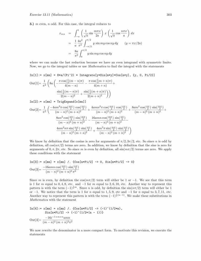
Exercise 13.11 (Mathematica) 303
3.) m even, n odd. For this case, the integral reduces to
xmn =
∫ a
−a
(1√a
sinmπx
2a
)x
(1√a
cosnπx
a
)dx
=1
a
4a2
π2
∫ π/2
−π/2y sinmy cosny dy (y = πx/2a)
=8a
π2
∫ π/2
0
y sinmy cosny dy
where we can make the last reduction because we have an even integrand with symmetric limits.Now, we go to the integral tables or use Mathematica to find the integral with the statements
In[1]:= x[mn] = 8*a/(Pi^2) * Integrate[y*Sin[m*y]*Cos[n*y], y, 0, Pi/2]
Out[1]=1
π2
(8a
(−π cos( 1
2 (m− n)π)
4(m− n)−π cos( 1
2m+ n)π)
4(m+ n)+
sin( 12 (m− n)π)
2(m− n)2+
sin( 12 (m+ n)π)
2(m+ n)2
))In[2]:= x[mn] = TrigExpand[x[mn]]
Out[2]=1
π2
(−4am3π cos(mπ2 ) cos(nπ2 )
(m− n)2 (m+ n)2+
4amn2π cos(mπ2 ) cos(nπ2 )
(m− n)2 (m+ n)2+
8am2 cos(nπ2 ) sin(mπ2 )
(m− n)2 (m+ n)2+
8an2 cos(nπ2 ) sin(mπ2 )
(m− n)2 (m+ n)2−
16amn cos(mπ2 ) sin(nπ2 )
(m− n)2 (m+ n)2−
4am2nπ sin(mπ2 ) sin(nπ2 )
(m− n)2 (m+ n)2+
4an3π sin(mπ2 ) sin(nπ2 )
(m− n)2 (m+ n)2
)We know by definition that the cosine is zero for arguments of π/2, 3π/2, etc. So since n is odd bydefinition, all cos(nπ/2) terms are zero. In addition, we know by definition that the sine is zero forarguments of 0, π, 2π, etc. So since m is even by definition, all sin(mπ/2) terms are zero. We applythese conditions with the statement
In[3]:= x[mn] = x[mn] /. Cos[n*Pi/2] -> 0, Sin[m*Pi/2] -> 0
Out[3]=−16amn cos(mπ2 ) sin(nπ2 )
(m− n)2 (m+ n)2 π2
Since m is even, by definition the cos(mπ/2) term will either be 1 or −1. We see that this termis 1 for m equal to 0, 4, 8, etc. and −1 for m equal to 2, 6, 10, etc. Another way to represent thispattern is with the term (−1)
12m. Since n is odd, by definition the sin(nπ/2) term will either be 1
or −1. We notice that the term is 1 for n equal to 1, 5, 9, etc and −1 for n equal to 3, 7, 11, etc.Another way to represent this pattern is with the term (−1)
12 (n−1). We make these substitutions in
Mathematica with the statement
In[4]:= x[mn] = x[mn] /. Cos[m*Pi/2] -> (-1)^(1/2*m),
Sin[n*Pi/2] -> (-1)^(1/2*(n - 1))
Out[4]=−16i−1+m+namn
(m− n)2 (m+ n)2π2
We now rewrite the denominator in a more compact form. To motivate this revision, we execute thestatements
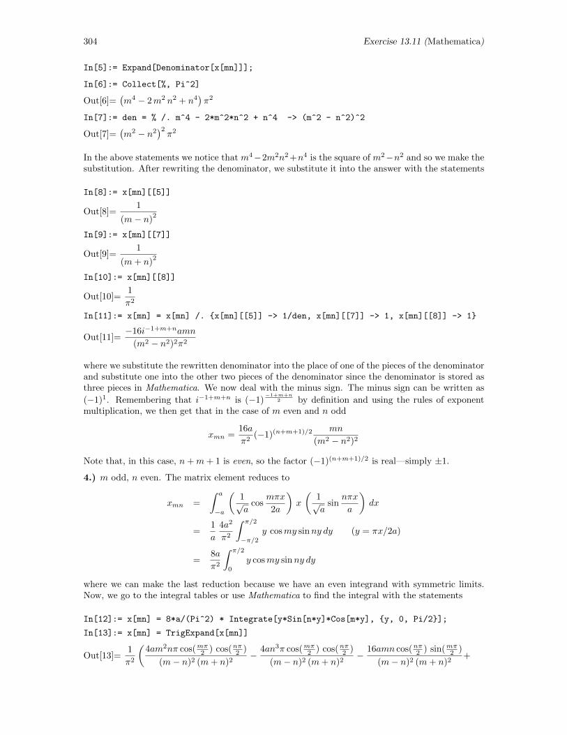
304 Exercise 13.11 (Mathematica)
In[5]:= Expand[Denominator[x[mn]]];
In[6]:= Collect[%, Pi^2]
Out[6]=(m4 − 2m2 n2 + n4
)π2
In[7]:= den = % /. m^4 - 2*m^2*n^2 + n^4 -> (m^2 - n^2)^2
Out[7]=(m2 − n2
)2π2
In the above statements we notice that m4−2m2n2 +n4 is the square of m2−n2 and so we make thesubstitution. After rewriting the denominator, we substitute it into the answer with the statements
In[8]:= x[mn][[5]]
Out[8]=1
(m− n)2
In[9]:= x[mn][[7]]
Out[9]=1
(m+ n)2
In[10]:= x[mn][[8]]
Out[10]=1
π2
In[11]:= x[mn] = x[mn] /. x[mn][[5]] -> 1/den, x[mn][[7]] -> 1, x[mn][[8]] -> 1
Out[11]=−16i−1+m+namn
(m2 − n2)2π2
where we substitute the rewritten denominator into the place of one of the pieces of the denominatorand substitute one into the other two pieces of the denominator since the denominator is stored asthree pieces in Mathematica. We now deal with the minus sign. The minus sign can be written as
(−1)1. Remembering that i−1+m+n is (−1)−1+m+n
2 by definition and using the rules of exponentmultiplication, we then get that in the case of m even and n odd
xmn =16a
π2(−1)(n+m+1)/2 mn
(m2 − n2)2
Note that, in this case, n+m+ 1 is even, so the factor (−1)(n+m+1)/2 is real—simply ±1.
4.) m odd, n even. The matrix element reduces to
xmn =
∫ a
−a
(1√a
cosmπx
2a
)x
(1√a
sinnπx
a
)dx
=1
a
4a2
π2
∫ π/2
−π/2y cosmy sinny dy (y = πx/2a)
=8a
π2
∫ π/2
0
y cosmy sinny dy
where we can make the last reduction because we have an even integrand with symmetric limits.Now, we go to the integral tables or use Mathematica to find the integral with the statements
In[12]:= x[mn] = 8*a/(Pi^2) * Integrate[y*Sin[n*y]*Cos[m*y], y, 0, Pi/2];
In[13]:= x[mn] = TrigExpand[x[mn]]
Out[13]=1
π2
(4am2nπ cos(mπ2 ) cos(nπ2 )
(m− n)2 (m+ n)2−
4an3π cos(mπ2 ) cos(nπ2 )
(m− n)2 (m+ n)2−
16amn cos(nπ2 ) sin(mπ2 )
(m− n)2 (m+ n)2+
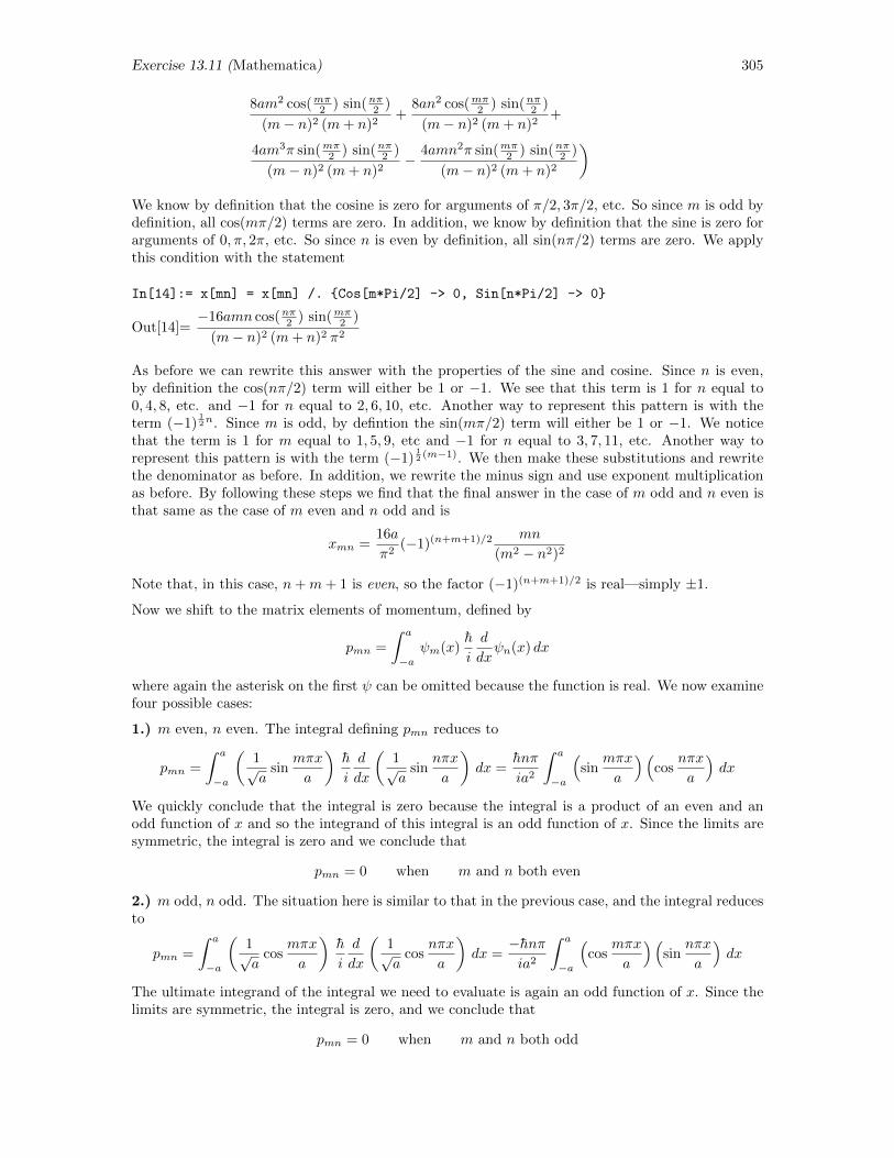
Exercise 13.11 (Mathematica) 305
8am2 cos(mπ2 ) sin(nπ2 )
(m− n)2 (m+ n)2+
8an2 cos(mπ2 ) sin(nπ2 )
(m− n)2 (m+ n)2+
4am3π sin(mπ2 ) sin(nπ2 )
(m− n)2 (m+ n)2−
4amn2π sin(mπ2 ) sin(nπ2 )
(m− n)2 (m+ n)2
)We know by definition that the cosine is zero for arguments of π/2, 3π/2, etc. So since m is odd bydefinition, all cos(mπ/2) terms are zero. In addition, we know by definition that the sine is zero forarguments of 0, π, 2π, etc. So since n is even by definition, all sin(nπ/2) terms are zero. We applythis condition with the statement
In[14]:= x[mn] = x[mn] /. Cos[m*Pi/2] -> 0, Sin[n*Pi/2] -> 0
Out[14]=−16amn cos(nπ2 ) sin(mπ2 )
(m− n)2 (m+ n)2 π2
As before we can rewrite this answer with the properties of the sine and cosine. Since n is even,by definition the cos(nπ/2) term will either be 1 or −1. We see that this term is 1 for n equal to0, 4, 8, etc. and −1 for n equal to 2, 6, 10, etc. Another way to represent this pattern is with theterm (−1)
12n. Since m is odd, by defintion the sin(mπ/2) term will either be 1 or −1. We notice
that the term is 1 for m equal to 1, 5, 9, etc and −1 for n equal to 3, 7, 11, etc. Another way torepresent this pattern is with the term (−1)
12 (m−1). We then make these substitutions and rewrite
the denominator as before. In addition, we rewrite the minus sign and use exponent multiplicationas before. By following these steps we find that the final answer in the case of m odd and n even isthat same as the case of m even and n odd and is
xmn =16a
π2(−1)(n+m+1)/2 mn
(m2 − n2)2
Note that, in this case, n+m+ 1 is even, so the factor (−1)(n+m+1)/2 is real—simply ±1.
Now we shift to the matrix elements of momentum, defined by
pmn =
∫ a
−aψm(x)
h
i
d
dxψn(x) dx
where again the asterisk on the first ψ can be omitted because the function is real. We now examinefour possible cases:
1.) m even, n even. The integral defining pmn reduces to
pmn =
∫ a
−a
(1√a
sinmπx
a
)h
i
d
dx
(1√a
sinnπx
a
)dx =
hnπ
ia2
∫ a
−a
(sin
mπx
a
)(cos
nπx
a
)dx
We quickly conclude that the integral is zero because the integral is a product of an even and anodd function of x and so the integrand of this integral is an odd function of x. Since the limits aresymmetric, the integral is zero and we conclude that
pmn = 0 when m and n both even
2.) m odd, n odd. The situation here is similar to that in the previous case, and the integral reducesto
pmn =
∫ a
−a
(1√a
cosmπx
a
)h
i
d
dx
(1√a
cosnπx
a
)dx =
−hnπia2
∫ a
−a
(cos
mπx
a
)(sin
nπx
a
)dx
The ultimate integrand of the integral we need to evaluate is again an odd function of x. Since thelimits are symmetric, the integral is zero, and we conclude that
pmn = 0 when m and n both odd
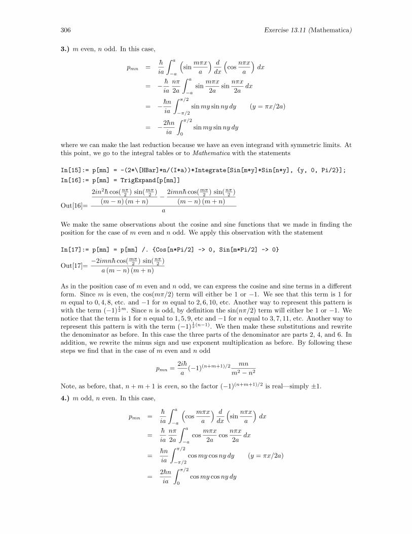
306 Exercise 13.11 (Mathematica)
3.) m even, n odd. In this case,
pmn =h
ia
∫ a
−a
(sin
mπx
a
) d
dx
(cos
nπx
a
)dx
= − hia
nπ
2a
∫ a
−asin
mπx
2asin
nπx
2adx
= − hnia
∫ π/2
−π/2sinmy sinny dy (y = πx/2a)
= −2hn
ia
∫ π/2
0
sinmy sinny dy
where we can make the last reduction because we have an even integrand with symmetric limits. Atthis point, we go to the integral tables or to Mathematica with the statements
In[15]:= p[mn] = -(2*\[HBar]*n/(I*a))*Integrate[Sin[m*y]*Sin[n*y], y, 0, Pi/2];
In[16]:= p[mn] = TrigExpand[p[mn]]
Out[16]=
2in2h cos(nπ2 ) sin(mπ2 )
(m− n) (m+ n)−
2imnh cos(mπ2 ) sin(nπ2 )
(m− n) (m+ n)
a
We make the same observations about the cosine and sine functions that we made in finding theposition for the case of m even and n odd. We apply this observation with the statement
In[17]:= p[mn] = p[mn] /. Cos[n*Pi/2] -> 0, Sin[m*Pi/2] -> 0
Out[17]=−2imnh cos(mπ2 ) sin(nπ2 )
a (m− n) (m+ n)
As in the position case of m even and n odd, we can express the cosine and sine terms in a differentform. Since m is even, the cos(mπ/2) term will either be 1 or −1. We see that this term is 1 form equal to 0, 4, 8, etc. and −1 for m equal to 2, 6, 10, etc. Another way to represent this pattern iswith the term (−1)
12m. Since n is odd, by definition the sin(nπ/2) term will either be 1 or −1. We
notice that the term is 1 for n equal to 1, 5, 9, etc and −1 for n equal to 3, 7, 11, etc. Another way torepresent this pattern is with the term (−1)
12 (n−1). We then make these substitutions and rewrite
the denominator as before. In this case the three parts of the denominator are parts 2, 4, and 6. Inaddition, we rewrite the minus sign and use exponent multiplication as before. By following thesesteps we find that in the case of m even and n odd
pmn =2ih
a(−1)(n+m+1)/2 mn
m2 − n2
Note, as before, that, n+m+ 1 is even, so the factor (−1)(n+m+1)/2 is real—simply ±1.
4.) m odd, n even. In this case,
pmn =h
ia
∫ a
−a
(cos
mπx
a
) d
dx
(sin
nπx
a
)dx
=h
ia
nπ
2a
∫ a
−acos
mπx
2acos
nπx
2adx
=hn
ia
∫ π/2
−π/2cosmy cosny dy (y = πx/2a)
=2hn
ia
∫ π/2
0
cosmy cosny dy
Exercise 13.11 (Mathematica) 307
where we can make the last reduction because we have an even integrand with symmetric limits. Atthis point, we go to the integral tables or to Mathematica with the statements
In[18]:= p[mn] = (2*\[HBar]*n/(I*a))*Integrate[Cos[m*y]*Cos[n*y], y, 0, Pi/2];
In[19]:= p[mn] = TrigExpand[p[mn]]
Out[19]=
−2imnh cos(nπ2 ) sin(mπ2 )
(m− n) (m+ n)+
2in2h cos(mπ2 ) sin(nπ2 )
(m− n) (m+ n)
a
We make the same observations about the cosine and sine functions that we made in finding theposition for the case of m odd and n even. We apply this observation with the statement
In[20]:= p[mn] = p[mn] /. Cos[m*Pi/2] -> 0, Sin[n*Pi/2] -> 0
Out[20]=2imnh cos(nπ2 ) sin(mπ2 )
a(m− n) (m+ n)
As in the position case of m odd and n even, we can express the cosine and sine terms in a differentform. We can represent the cosine with the term (−1)
12n and the sine with the term (−1)
12 (m−1).
We then make these substitutions and rewrite the denominator as before. In this case the threeparts of the denominator are parts 2, 4, and 6. By following these steps we find that in the case ofm odd and n even, just as in the case of m even and n odd,
pmn =2ih
a(−1)(n+m+1)/2 mn
m2 − n2
Note, as before, that, n+m+ 1 is even, so the factor (−1)(n+m+1)/2 is real—simply ±1.
308 Exercise 13.12 (Mathematica)
13.12 Fourier Coefficients for Sawtooth (Mathematica)
Exercise: The sawtooth wave is defined by
f(x) =x
l; −l ≤ x ≤ l
Use symbolic integration to find the Fourier coefficients an and bn for this function and then generategraphs showing the function given by the truncated series
ftrunc(x) =a0
2+
N∑n=1
(an cos
nπx
l+ bn sin
nπx
l
)for various values of N , including 0, 1, 2, 3, and 10.
Solution: For the sawtooth wave defined by
f(x) =x
l; −l ≤ x ≤ l
the Fourier coefficients, an and bn, are given by
an =1
l
∫ l
−lf(x) cos
nπx
ldx ; bn =
1
l
∫ l
−lf(x) sin
nπx
ldx
In terms of the variable x = x/l, these integrals become
an =
∫ 1
−1
x cos(nπx) dx ; bn =
∫ 1
−1
f(x) sin(nπx dx
Dropping the overbars, we find these coefficients in Mathematica using the statements
In[1]:= a[n_] := Integrate[ x*Cos[n*Pi*x], x,-1,1]
In[2]:= b[n_] := Integrate[ x*Sin[n*Pi*x], x,-1,1]
(Remember to use Pi not pi so Mathematica will know you mean the value as well as the symbol.)
Our remaining task is to evaluate these coefficients for specific terms and generate plots for thetruncated function
ftrunc(x) =a0
2+
N∑n=1
(an cos
nπx
l+ bn sin
nπx
l
)=a0
2+
N∑n=1
(an cos(nπx) + bn sin(nπx))
for N = 1, 2, 3 and 10. We evaluate the sum for these four cases and create the plots with thestatements
In[3]:= ftrunc1 = a[0]/2 + Sum[ a[n]*Cos[n*Pi*x]+b[n]*Sin[n*Pi*x], n, 0, 1 ];
In[4]:= Plot[ftrunc1, x, -2.5, 2.5, PlotRange->-1.2,1.2,
PlotPoints->250, PlotStyle->Thickness[0.01] ]
In[5]:= ftrunc2 = a[0]/2 + Sum[ a[n]*Cos[n*Pi*x] + b[n]*Sin[n*Pi*x], n, 0, 2 ];
In[6]:= Plot[ftrunc2, x, -2.5, 2.5, PlotRange->-1.2,1.2,
PlotPoints->250, PlotStyle->Thickness[0.01] ]
In[7]:= ftrunc3 = a[0]/2 + Sum[a[n]*Cos[n*Pi*x] + b[n]*Sin[n*Pi*x], n, 0, 3 ];
In[8]:= Plot[ftrunc3, x, -2.5, 2.5, PlotRange->-1.2,1.2,
PlotPoints->250, PlotStyle->Thickness[0.01] ]
In[9]:= ftrunc10 = a[0]/2 + Sum[a[n]*Cos[n*Pi*x] + b[n]*Sin[n*Pi*x], n, 0, 10 ];
In[10]:= Plot[ftrunc10, x, -2.5, 2.5, PlotRange->-1.2,1.2,
PlotPoints->250, PlotStyle->Thickness[0.01] ]
The plots in Figs. 13.3–13.6 get progressively sharper and more like a sawtooth as the number ofterms in the Fourier series increases.
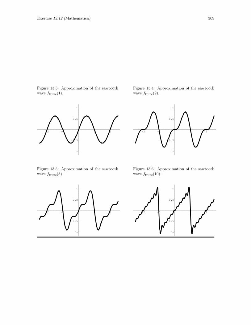
Exercise 13.12 (Mathematica) 309
Figure 13.3: Approximation of the sawtoothwave ftrunc(1).
-2 -1 1 2
-1
-0.5
0.5
1
Figure 13.4: Approximation of the sawtoothwave ftrunc(2).
-2 -1 1 2
-1
-0.5
0.5
1
Figure 13.5: Approximation of the sawtoothwave ftrunc(3).
-2 -1 1 2
-1
-0.5
0.5
1
Figure 13.6: Approximation of the sawtoothwave ftrunc(10).
-2 -1 1 2
-1
-0.5
0.5
1
310 Exercise 13.13 (MATHEMATICA)
13.13 Expansion in Legendre Polynomials (MATHEMAT-ICA)
Exercise: The Legendre polynomials Ln(x), n = 0, 1, 2, . . ., are orthogonal on the interval−1 ≤ x ≤ 1 with weight 1. In particular,∫ 1
−1
Lm(x)Ln(x) dx =2
2n+ 1δmn
Any function defined over the interval −1 ≤ x ≤ 1 can then be expanded in the Legendre series
f(x) =
∞∑n=0
cn Ln(x)
(a) Show by hand that the coefficient cn in this expansion is given by
cn =2n+ 1
2
∫ 1
−1
f(x)Ln(x) dx
(b) Use symbolic integration to find cn for n = 0, 1, 2, 3, 4, 5 and 6 in the Legendre expansion for thefunction
f(x) =
−1 −1 < x < 0
1 0 < x < 1
(c) Graph the functions defined by the partial sums∑Nn=0 cn Ln(x) for N = 0, 1, 2, 3, 4, 5, and 6.
Hint : Quite possibly the symbolic program you are using has the Legendre polynomials builtin somehow, and you should study its manuals to find out how to invoke them. Just in case thatisn’t true, the first nine Legendre polynomials are
L0(x) = 1 L5(x) = 18 (63x5 − 70x3 + 15x)
L1(x) = x L6(x) = 116 (231x6 − 315x4 + 105x2 − 5)
L2(x) = 12 (3x2 − 1) L7(x) = 1
16 (429x7 − 693x5 + 315x3 − 35x)
L3(x) = 12 (5x3 − 3x) L8(x) = 1
128 (6435x8 − 12012x6 + 6930x4 − 1260x2 + 35)
L4(x) = 18 (35x4 − 30x2 + 3) L9(x) = 1
128 (12155x9 − 25740x7 + 18018x5 − 4620x3 + 315x)
Solution: (a) To solve this part of the exercise, we multiply the second equation in the problemstatement by Lm(x) and integrate over the interval −1 ≤ x ≤ 1 to find that∫ 1
−1
Lm(x) f(x) ds =∑n
cn
∫ 1
−1
Ln(x)Lm(x) dx =∑n
cn
(2
2n+ 1δmn
)= cm
(2
2m+ 1
)Here we have recognized the orthogonality of the polynomials as given in the first equation in thestatement of the exercise. We conclude that
cn =2n+ 1
2
∫ 1
−1
Ln(x) f(x) dx
(b) The first thing we can notice about this function is that it is odd, i.e. f(−x) = −f(x). Recallingthe properties of even and odd functions, we know also that two odd functions multiplied togetherwill produce an even function, while one of each will produce an odd function. This proves usefulbecause Ln(x) is even when n is even, and odd when n is odd. Therefore, gn(x) = f(x)Ln(x) will beodd when n is even and even when n is odd. Since odd functions integrated over symmetric limitswill be zero, we only care therefore about the even functions gn(x) = f(x)Ln(x), when n is odd.
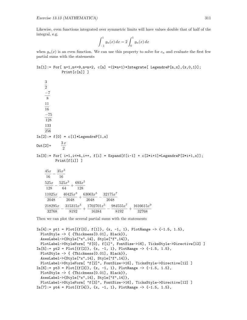
Exercise 13.13 (MATHEMATICA) 311
Likewise, even functions integrated over symmetric limits will have values double that of half of theintegral, e.g. ∫ 1
−1
gn(x) dx = 2
∫ 1
0
gn(x) dx
when gn(x) is an even function. We can use this property to solve for cn and evaluate the first fewpartial sums with the statements
In[1]:= For[ n=1,n<=9,n=n+2, c[n] =(2*n+1)*Integrate[ LegendreP[n,x],x,0,1];
Print[c[n]] ]
3
2
−7
8
11
16
−75
128
133
256
In[2]:= f[0] = c[1]*LegendreP[1,x]
Out[2]=3x
2
In[3]:= For[ i=1,i<=4,i++, f[i] = Expand[f[i-1] + c[2*i+1]*LegendreP[2*i+1,x]];
Print[f[i]] ]
45x
16− 35x3
16
525x
128− 525x3
64+
693x5
128
11025x
2048− 40425x3
2048+
63063x5
2048− 32175x7
2048
218295x
32768− 315315x3
8192+
1702701x5
16384− 984555x7
8192+
1616615x9
32768
Then we can plot the several partial sums with the statements
In[4]:= pt1 = Plot[f[0], f[1], x, -1, 1, PlotRange -> -1.5, 1.5,
PlotStyle -> Thickness[0.01], Black,
AxesLabel->Style["x",14], Style["f",14],
PlotLabel->StyleForm[ "f[0], f[1]", FontSize->16], TicksStyle->Directive[12] ]
In[5]:= pt2 = Plot[f[2], x, -1, 1, PlotRange -> -1.5, 1.5,
PlotStyle -> Thickness[0.01], Black,
AxesLabel->Style["x",14], Style["f",14],
PlotLabel->StyleForm[ "f[2]", FontSize->16], TicksStyle->Directive[12] ]
In[6]:= pt3 = Plot[f[3], x, -1, 1, PlotRange -> -1.5, 1.5,
PlotStyle -> Thickness[0.01], Black,
AxesLabel->Style["x",14], Style["f",14],
PlotLabel->StyleForm[ "f[3]", FontSize->16], TicksStyle->Directive[12] ]
In[7]:= pt4 = Plot[f[4], x, -1, 1, PlotRange -> -1.5, 1.5,
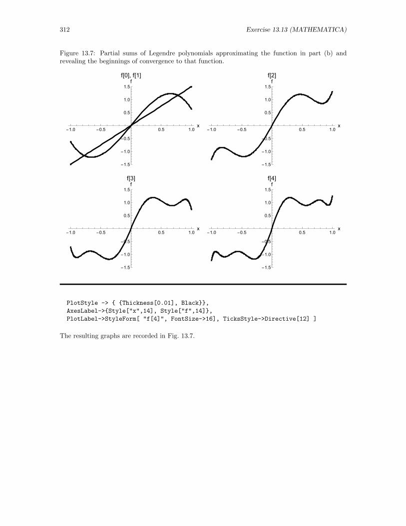
312 Exercise 13.13 (MATHEMATICA)
Figure 13.7: Partial sums of Legendre polynomials approximating the function in part (b) andrevealing the beginnings of convergence to that function.
-1.0 -0.5 0.5 1.0x
-1.5
-1.0
-0.5
0.5
1.0
1.5f
f[0], f[1]
-1.0 -0.5 0.5 1.0x
-1.5
-1.0
-0.5
0.5
1.0
1.5ff[2]
-1.0 -0.5 0.5 1.0x
-1.5
-1.0
-0.5
0.5
1.0
1.5ff[3]
-1.0 -0.5 0.5 1.0x
-1.5
-1.0
-0.5
0.5
1.0
1.5ff[4]
PlotStyle -> Thickness[0.01], Black,
AxesLabel->Style["x",14], Style["f",14],
PlotLabel->StyleForm[ "f[4]", FontSize->16], TicksStyle->Directive[12] ]
The resulting graphs are recorded in Fig. 13.7.
Exercise 13.14 (Mathematica) 313
13.14 Deduction of Simpson’s Rule (Mathematica)
Exercise: To deduce Simpson’s rule, we start by supposing three consecutive values f1, f2,and f3 of the integrand, where for simplicity in notation we take the points of evaluation to bex1 = x2 − ∆x, x2, and x3 = x2 + ∆x. Using a symbol manipulating program to do the algebraand calculus, (a) find the coefficients A, B, and C needed to make the parabola Ax2 +Bx+C passthrough the three points (xi, fi), i = 1, 2, 3, (b) integrate that parabola over the interval x1 < x < x3
to find that ∫ x3
x1
f(x) dx ≈∫ x3
x1
(Ax2 +Bx+ C) dx =∆x
3
(f1 + 4f2 + f3
)(c) show that this result actually gives the correct value for f(x) = x3 and, finally, (d) deduce the(extended) Simpson’s rule∫ b
a
f(x) dx ≈ SN = 13 (f0 + 4f1 + 2f2 + 4f3 + · · ·+ 2fN−2 + 4fN−1 + fN ) ∆x
Note: Because this exercise relates to numerical algorithms, it has been placed in with other exercisesthat are numerical. This exercise is symbolic, and you should use a symbol manipulating programfor parts (a), (b), and (c); however, you should address part (d) by hand.
Solution: (a), (b) We want to begin by fitting the parabola
f(x) = Ax2 +Bx+ C
to the three points
f(x2 −∆x) = f1 ; f(x2) = f2 ; f(x2 + ∆x) = f3
Using Mathematica, we first define the general function f(x) with the statement
In[1]:= f[x_] := A*x^2+B*x+C;
Then, we stipulate that the three points shall lie on the parabola by defining the three equations
In[2]:= eq1 = f1 == f[x2-dx];
In[3]:= eq2 = f2 == f[x2];
In[4]:= eq3 = f3 == f[x2+dx];
Next, we solve the three equations for the constants A, B, and C with the statement
In[5]:= soln = Solve[ eq1, eq2, eq3, A, B, C ][[1]]
Out[5]= :=A→ . . . , B → . . . , C → . . .
though we suppress the explicit solutions because of their complexity. Finally, we substitute thissolution into the original function and integrate it with the statements
In[6]:= integ = f[x] /. soln:
In[7]:= S = Integrate[ integ, x, x2-dx, x2+dx ]:
In[8]:= S = Simplify[ S ]
Out[8]= :=dx
3
(f1 + 4f2 + f3
)which demonstrates the correctness of the desired relationship.
(c) For the cubic polynomial g(x) = x3, we use the statements
314 Exercise 13.14 (Mathematica)
In[9]:= g[x_] = x^3;
In[10]:= S /. f1 -> g[x2-dx], f2 -> g[x2], f3 -> g[x2+dx];
In[11]:= Simplify[ % ]
Out[11]= 2 dxx2(dx2 + x22)
to find∫ x2+dx
x2−dx g(x) dx via Simpson’s rule and the statements
In[12]:= Integrate[ g[x], x, x2-dx, x2+dx ];
In[13]:= Simplify[ % ]
2 dxx2(dx2 + x22)
to evaluate the same integral formally and exactly. We do indeed discover that Simpson’s rule, whichwas designed to be exactly correct for quadratic polynomials is apparently also exactly correct forthe cubic function!
(d) To deduce the extended Simpson’s rule, let us introduce the points xi = i∆x, i = 0, 1, 2, . . . , N ,with a = x0 and b = xN . Make sure N is even, so we have an integer number of pairs or strips.Then, we write
∫ b
a
f(x) dx =
N/2∑i=0
∫ x2i+2
x2i
f(x) dx
=
∫ x2
x0
f(x) dx+
∫ x4
x2
f(x) dx+ · · ·+∫ xN−2
xN−4
f(x) dx+
∫ xN
xN−2
f(x) dx
=dx
3
((f0 + 4f1 + f2) + f2 + 4f3 + f4) + · · ·
+(fN−4 + 4fN−3 + fN−2) + (fN−2 + 4fN−1 + fN ))
=dx
3
(f0 + 4f1 + 2f2 + 4f3 + 2f4 + · · ·+ 2fN−4 + 4fN−3 + 2fN−2 + 4fN−1 + fN
)where, in this last expression (which was obtained by substituting appropriate values into the resultof part (b)), fi = f(xi). Q.E.D.
Exercise 13.18 (IDL) 315
13.18 Quantum Harmonic Oscillator Turning Points (IDL)
Exercise: The (normalized) wave functions for a quantum harmonic oscillator in its first andsecond excited states (n = 1, n = 2) are
ψ1(x) =√
2(mωπh
)1/4
ye−y2/2 ; ψ2(x) =
1√2
(mωπh
)1/4 (2y2 − 1
)e−y
2/2
where y = x/a, a =√hω/k, and ω =
√k/m.
Solution: The energies of these states are 3hω/2 and 5hω/2, respectively. We know that theclassical turning point occurs when the potential energy, kx2/2, is equal to the energy of the state, sowe find that x1turn =
√3hω/k =
√3 a and x2turn =
√5hω/k =
√5 a. Now, to find the probability
that the oscillator will be outside the classical turning point, we need to subtract the integral from−xturn to xturn of the square magnitude of the wave function from the total probability of findingthe oscillator somewhere, i.e., from 1. Thus, we conclude that
P1 = 1−∫ x=
√3 a
x=−√
3
|ψ1(x)|2 dx = 1− 2
√mω
πh
∫ y=√
3
y=−√
3
y2e−y2
d(ay)
= 1− 2
√ma2ω
πh
∫ √3
−√
3
y2e−y2
dy = 1− 2√π
∫ √3
−√
3
y2e−y2
dy
= 1− 4√π
∫ √3
0
y2e−y2
dy
and
P2 = 1−∫ x=
√5 a
x=−√
5 a
|ψ2(x)|2 dx = 1− 1
2
√mω
πh
∫ y=√
5
y=−√
5
(2y2 − 1)2e−y2
d(ay)
= 1− 1
2
√ma2ω
πh
∫ √5
−√
5
(2y2 − 1)2e−y2
dy = 1− 1
2√π
∫ √5
−√
5
(2y2 − 1)2e−y2
dy
= 1− 1√π
∫ √5
0
(2y2 − 1)2e−y2
dy
where the last form in each case emerges when we recognize that the integrand is an even functionof y and the limits are symmetric. The necessary function pro-files then are:
FUNCTION quantumn1, y
Part1 = 4.0/sqrt(!pi)
RETURN, Part1*y^2*exp(-y^2)
END
and
FUNCTION quantumn2, y
Part1 = 1.0/sqrt(!pi)
RETURN, Part1*(2*y^2-1)^2*exp(-y^2)
END
After these files have been saved in the default directories with the names quantumn1.pro andquantumn2.pro, we can evaluate the desired integrals by invoking the function luqsimp with thestatements

316 Exercise 13.18 (IDL)
IDL> n1 = 1 - luqsimp( ’quantumn1’, 0.0, sqrt(3.0), eps=0.00001 )
% Compiled module: LUQSIMP.
% Compiled module: TRAPZD.
% Compiled module: QUANTUMN1.
IDL> print, n1
0.11161021
IDL> n2 = 1 - luqsimp( ’quantumn2’, 0.0, sqrt(5.0), eps=0.000001 )
% Compiled module: QUANTUMN2.
IDL> print, n2
0.095069447
We learn that the oscillator will be outside the classical turning point 11.16% of the time when it isin its first excited state and 9.51% of the time when it is in the second excited state.
Exercise 13.19 (IDL) 317
13.19 Maxwell-Boltzmann Distribution (IDL)
Exercise: The Maxwell-Boltzmann speed distribution yields the integral
f(v) = 4π( m
2πkT
) 32
∫ v
0
e−mv′2/2kT v′2 dv′
for the fraction of the molecules having speed less than v. Using numerical means, explore thisintegral as a function of v. Hint : Re-express the integral using
√2kT/m as the unit of velocity.
Solution: The Maxwell-Boltzmann speed distribution gives us the integral
f(v) = 4π( m
2πkT
) 32
∫ v
0
e−mv′2/2kT v′2 dv′
for the fraction of molecules having speed less than v. By letting X =√v2m/2kT , and therefore
dX =√m/kTdv, we can recast this integral as
f(X) =4√π
∫ X
0
e−X′2X ′2 dX ′
To evaluate this integral in IDL, we begin by creating the function pro-file
function maxbolt, x
;
; The Maxwell-Boltzmann speed distribution
; in dimensionless form, x=v/sqrt(2kT/m).
;
return, x^2*exp(-x^2)
end
that will return the integrand. Once the pro-file is written and saved in the default directory withthe name maxbolt.pro, we can evaluate the integral by invoking the IDL procedure luqsimp withthe statements
IDL> x = findgen(31)/10.0
IDL> q = size(x) & N=q[1]-1
IDL> mb = fltarr(N+1)
IDL> for i=0, N do mb[i] = 4/sqrt(!pi)*luqsimp("maxbolt", 0.0, x[i])
IDL> plot, x, mb, title=’Speed Distribution’, $
IDL> xtitle=’X’, ytitle=’f(X)’
The resulting graph is shown in Fig. 13.8. As expected (since more and more molecules are includedas v increases), this graph approaches 1 as X = v/
√m/2kT approaches infinity.
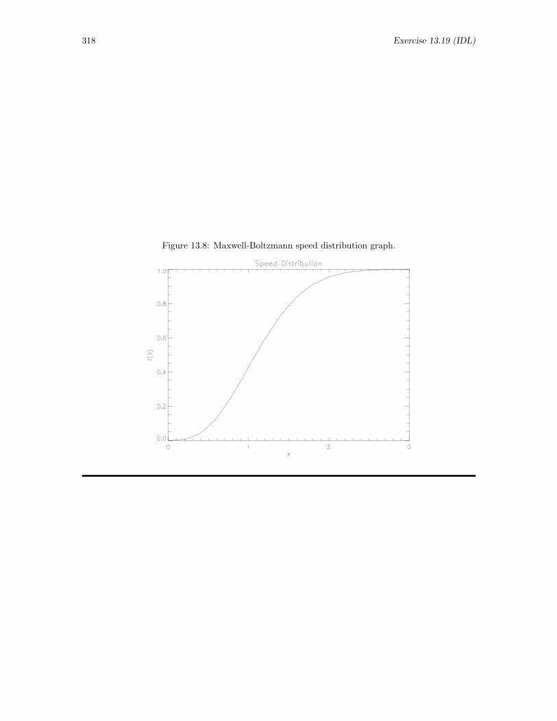
318 Exercise 13.19 (IDL)
Figure 13.8: Maxwell-Boltzmann speed distribution graph.
Exercise 13.20 (IDL) 319
13.20 Black Body Radiation (IDL)
Exercise: Planck’s black body radiation law gives the expression
I(ν2, ν1) =8πh
c3
∫ ν2
ν1
ν3
ehν/kT − 1dν
for the power radiated per unit area in the frequency range ν1 ≤ ν ≤ ν2. Using numerical means,explore the power radiated in the visible spectrum 4× 10¹⁴ Hz ≤ ν ≤ 7× 10¹⁴ Hz as a function oftemperature. Hint : One way to approach this exercise would be to choose a reference frequency ν0
arbitrarily (say 1014 Hz) and recast the integral on the dimensionless variable s = ν/ν0. Examinationof I in units of 8πhν4
0/c3 as a function of T in units of hν0/k would then be indicated.
Solution: Planck’s black body radiation law gives us the expression
I =8πh
c3
∫ ν2
ν1
ν3
ehv/kT − 1dν
for the power radiated per unit area over the frequency range ν1 ≤ ν ≤ ν2. Introducing thedimensionless variable s = ν/ν0 (where ν0 is an arbitrarily selected reference frequency) and notingthat ds = dν/ν0, we can recast this equation as
I =8πhν4
0
c3
∫ ν2/ν0
ν1/ν0
s3
ehsν0/kT − 1ds
If we express I in units of I0 = 8πhν40/c
3 as a function of T in units of T0 = hν0/k, then we have
I ′ =
∫ ν2/ν0
ν1/ν0
s3
es/T ′ − 1ds
where I ′ = I/(8πhν40/c
3) and T ′ = T/(hν0/k). To explore this integral over the frequency range4×1014 Hz ≤ ν ≤ 7×10¹⁴ Hz, let us choose the reference frequency to be 1014 Hz so that the integralof interest ranges from 4 to 7. Note also that this choice of ν0 implies the reference temperature
T0 =hν0
k=
6.62× 10−34 Js× 1014 s
1.38× 10⁻²³ J/K= 4797 K
Since the temperature of a white-hot tungsten filament is about 2800 K and the average temperatureof the sun is 5000-6000 K, the region of interest for this exercise probably is in the region of T/T0 ≤ 1.
The first step in exploring this integral is to write the function pro-file
function planck, s
;
; This pro-file returns the integrand
; for the power radiated per unit area
; according to Planck’s black body
; radiation law.
;
common param, t
den=exp(s/t)-1.0
return, (s^3)/den
end
to return the integrand of the integral of concern.
Then, in IDL, we establish the common parameter t, generate values for t within a reasonablerange, and invoke luqsimp to evaluate the integral for values of T ′ ranging from 0.0 to 2.0, an endaccomplished with the statements
320 Exercise 13.20 (IDL)
IDL> common param, t
IDL> tt=findgen(101)/50.0
IDL> q-size(tt) & N=q[1]-1
IDL> p = fltarr(N+1)
IDL> for i=0,N do begin $
IDL> t= tt[i] & $
IDL> p[i]=luqsimp("planck", 4.0, 7.0 ) & end
At this point, however, we discover that some sort of problem exists, because the attempt tointegrate yields a quick error message—a message which is not all that transparent but that doesremind us that the storage of sinble-precision values in IDL has a limited range. Further, we recallthat exponentials have a way of causing floating point under or overflow. Given the integral we areevaluating, the worst point in this regard will be at the upper limit, when the integrand involves theexponential e7.0/T ′ . At T ′ = 0, this exponential will definitely cause difficulties, since it will have thevalue e∞—a clear case of floating point overflow. We must, in fact, avoid evaluating the integrandat temperatures for which e7.0/T ′ exceeds about 1038. We find the critical value by searching withMATLAB, using the statements
IDL> print, exp(7.0/0.10)
2.51544e+30
IDL> print, exp(7.0/0.09)
6.00422e+33
IDL> print, exp(7.0/0.08)
1.00177e+38
IDL> print, exp(7.0/0.07)
Inf
Thus, we must make sure not to evaluate the integral for temperatures closer to zero than aboutT ′ = 0.07, since the numerical operation will be terminated with an error message at such points.We know, however, that the required intensity is actually quite small at the temperatures that willhere cause troubles. Thus, we can evaluate the integral for temperatures exceeding, say, 0.10 andfill in the values for smaller temperatures by taking them to be zero.
With that background, we are then motivated to revise the above procedure so that it starts atT/T0 = 0.10 and runs upwards to T/T0 = 2.0. The ppropriate statements are
IDL> common param, t
IDL> tt = findgen(96)/50.0 + 0.10
IDL> q = size(tt) & N = q[1]-1
IDL> p = fltarr(N+1)
IDL> for i = 1, N do begin $
IDL> t - tt[i] & $
IDL> p[i] = luqsimp( "planck", 4.0, 7.0 ) & end
IDL> plot, tt, p, title=’Black Body Radiation Intensity’, thick=3, $
stitle-’T/T0’, ytitle=’Intensity in the Visible/I0’
IDL> oplot, [0.0,m0.10, [0.0,0.0] thick=3
The resulting graph is shown in Fig. 13.9.
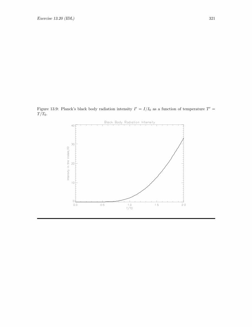
Exercise 13.20 (IDL) 321
Figure 13.9: Planck’s black body radiation intensity I ′ = I/I0 as a function of temperature T ′ =T/T0.
322 Exercise 13.21 (IDL)
13.21 Confidence Intervals for Gaussian (IDL)
Exercise: As used in statistical data analysis, the Gaussian distribution for a variable t isusually expressed in terms of the standard deviation σ, the distribution function being
1√2π σ
e−t2/2σ2
Thus, the probability of finding a value between a and b is given by
P (a, b) =1√2πσ
∫ b
a
e−t2/(2σ2) dt
Show analytically that P (−x, x) = erf(x/(√
2σ)), and then evaluate P (−σ, σ), P (−2σ, 2σ), andP (−3σ, 3σ) numerically. The values of these three quantities are 0.6827, 0.9545, and 0.9973,respectively—values that give rise to the designations of 68%, 95%, and 99% confidence intervals instatistical data analysis.
Solution: The probability that a single measurement drawn from a normally distributed uni-verse of possible values will lie between a and b is given by the integral
P (a, b) =1√2πσ
∫ b
a
e−t2/(2σ2) dt
To show analytically that P (−x, x) = erf(x/(√
2σ)), we simply change variables. If we let t2/2σ2 =s2, then dt =
√2σ ds and, when t = x, s = x/
√2σ. Thus, the integral becomes
P (−x, x) =1√π
∫ x/√
2σ
−x/√
2σ
e−s2
ds =2√π
∫ x/√
2σ
0
e−s2
ds = erf
(x√2σ
)The first equality is a result of the change of variables. The second stems from the observations that(1) the integrand is an even function of the integration variable and (2) the limits are symmetric.
To evaluate the error function for different values of x, we first create and store the functionpro-file
function erf, s
;
; This pro-file returns the integrand for the error function.
;
return, exp(-s^2)
end
to return the integrand. Then, since we seek specifically the values
P (−σ, σ) = erf
(1√2
); P (−2σ, 2σ) = erf
(2√2
); P (−3σ, 3σ) = erf
(3√2
)we invoke luqsimp in IDL and print the desired values with the statements
IDL> q=luqsimp("erf", 0.0, 1/sqrt(2.0))
IDL> qerf=(2/(sqrt(!pi))*q
IDL> print, qerf
0.682689
IDL> q=luqsimp("erf", 0.0, 2/sqrt(2.0))
IDL> qerf=(2/(sqrt(!pi))*q

Exercise 13.21 (IDL) 323
IDL> print, qerf
0.954500
IDL> q=luqsimp("erf", 0.0, 3/sqrt(2.0))
IDL> qerf=(2/(sqrt(!pi))*q
IDL> print, qerf
0.997300
We have accepted the default tolerance incorporated in the IDL routine.
We conclude that a single value randomly selected from a Gaussian distribution stands a 68.3%chance of falling within one standard deviation of the mean, a 95.4% chance of falling within twostandard deviations, and a 99.7% chance of falling within three standard deviations.
324 Exercise 13.22 (IDL)
13.22 Earth Falling into Sun (IDL)
Exercise: Suppose some cataclysmic event stops the earth dead in its tracks and, responding tothe sun’s gravitational attraction, the earth falls into the sun. Using numerical integration, find thetime required for the earth to fall over the middle half of its journey to the sun. Expressed in years,what numerically is the value of this time for the earth-sun system? Hint : Since the gravitationalpotential is −GmM/x, conservation of energy yields
1
2m
(dx
dt
)2
−GmMx
= −GmMx0
=⇒ dx
dt= −√
2GM
√1
x− 1
x0
(The negative square root is taken because x, the distance to the sun, is known to be decreasing.)This expression then leads to the value
Tmidhalf =1√
2GM
∫ 3x0/4
x0/4
(1
x− 1
x0
)−1/2
dx
Hint : The evaluation will be simpler if you begin by recasting the problem in dimensionless terms,expressing lengths in units of x0 and times in units of
√x3
0/(2GM). To interpret the significanceof this unit of time, determine the period of a circular orbit of radius x0, which will turn out to be2π√x3
0/GM . For the earth around the sun, this latter time is, of course, 1 year. Optional : Seeif you can develop a means to determine the time required for the first half of the journey, whichunfortunately—for numerical approaches—involves a convergent but improper integral.
Solution: Should the earth stop, the time it would take for it to fall over the middle half of itsjourney into the sun is given by the integral
Tmidhalf =1√
2GM
∫ 3x0/4
x0/4
(1
x− 1
x0
)−1/2
dx
To simplify the evaluation, let us introduce the dimensionless variable α = x/x0, so that the integralbecomes
Tmidhalf =
√x3
0
2GM
∫ 3/4
1/4
(1
α− 1
)−1/2
dα
To find a convenient time unit, let’s determine the period of a circular orbit at radius x0. We firstrequire that the gravitational force match the required centripetal force, i.e., that
mv2
x0=GmM
x20
=⇒ v =
√GM
x0
and then compute the period from the relationship
T0 =2πx0
v=
2πx0√GM/x0
=2πx
3/20√
GM
We conclude that, in this unit (where—for the earth around the sun—T0 is one year),
Tmidhalf
T0=
1
2π√
2
∫ 3/4
1/4
(1
α− 1
)−1/2
dα =1
2π√
2
∫ 3/4
1/4
√α
1− αdα
Note that the lower limit corresponds to the final position of the earth and the upper limit corre-sponds to the initial position of the earth.
To use IDL to evaluate this integral, we must first create an appropriate pro-file to define theintegrand, say the file
Exercise 13.22 (IDL) 325
FUNCTION earthfall, alpha
RETURN, sqrt(alpha/(1.0-alpha))/(2.0*!pi*sqrt(2))
END
We store this file with the name earthfall.pro in the default directory. Then we invoke luqsimp
with the following statement
IDL> print, luqsimp( ’earthfall’, 0.25, 0.75 )
0.058925565
which, given the default (fractional) tolerance of 10−6, we conclude is accurate to at least five digitsafter the decimal point. Recognizing that the time unit is one year for the earth, we conclude thatthe earth would take 0.058926 years (about 21.51 days or one month) to fall over the middle half ofits journey to the sun.
While we have the routine in hand, let’s note that the time required to fall over the last half ofits journey (from α = 0.5 to α = 0.0) would be
IDL> print, luqsimp( ’earthfall’, 0.0, 0.5 )
0.032118565
or about 11.8 days. The time required for the earth to fall over the last 90% of its journey would be
IDL> print, luqsimp( ’earthfall’, 0.0, 0.9 )
0.10680513
or about 38.98 days. Because the integrand diverges as α→ 1, we cannot reliably use this approachto find the time required for the earth’s entire journey to the sun. The integral is not a divergentintegral, but the divergence of the integrand precludes use of Simpson’s rule to obtain a reliableevaluation over intervals that extend too close to the starting point. We can, however, push theupper limit fairly close to 1.0 before IDL complains about non-convergence. For example, we findthat
IDL> print, luqsimp( ’earthfall’, 0.0, 0.99999 )
0.17606441
IDL> print, luqsimp( ’earthfall’, 0.0, 0.999999 )
% LUQSIMP: WARNING - Sum did not converge after 20 steps
0.17655328
IDL> print, luqsimp( ’earthfall’, 0.0, 0.999999, max_iter=40 )
0.17655011
The first of these values is about 64.26 days while the second and third are both about 64.44 days.Thus, we infer that, from start to finish, the entire calamity takes only about 64.4 days. (Theseresults can be compared with the analytic results obtained in Exercise 11.6.)
326 Exercise 13.23 (IDL)
13.23 Properties of Lorentz Distribution (IDL)
Exercise: The normalized Lorentz distribution function is given by
p(x) =1
π
a/2
x2 + (a/2)2
Find the probability that a single, randomly selected value will be in the range −a ≤ x ≤ a. Makesure to assess the precision of your result by methods that do not exploit a priori knowledge of theexact value. Hint : Before evaluating the integral, introduce the dimensionless variable s = x/a andnote that the result actually doesn’t depend on a, so there is but one number to determine.
Solution: The normalized Lorentz distribution function is
p(x) =1
π
a/2
x2 + (a/2)2
To find the probability that a single, randomly chosen value will be in the range −a ≤ x ≤ a, wemust integrate p(x)dx from −a to a. First, though, let us express x in a dimensionless form byintroducing the variable s = x/a. Since ds = dx/a, the new form of the integral is∫
p(s)ds =1
2π
∫ 1
−1
1
s2 + 1/4ds
To invoke luqsimp in IDL to evaluate the integral, we must write the function pro-file
function lorentz, s
;
; This program generates the integrand for
; the normalized Lorentz distribution, to be used in IDL.
; It is saved in the default directory as lorentz.pro.
;
tmp=1/(s^2+0.25)
return, tmp/(2*!pi)
end
to return the integrand. Once this program has been saved in a file named lorentz.pro, we canevaluate the integral in IDL with the statements
IDL> q=luqsimp("lorentz", -1.0, 1.0, eps=0.1) & print,q
0.70354646
IDL> q=luqsimp("lorentz", -1.0, 1.0, eps=0.01) & print,q
0.70482727
IDL> q=luqsimp("lorentz", -1.0, 1.0, eps=0.001) & print, q
0.70483256
IDL> q=luqsimp("lorentz", -1.0, 1.0, eps=0.0001) & print, q
0.70483256
IDL> q=luqsimp("lorentz", -1.0, 1.0, eps=0.00001) & print,q
0.70483256
IDL> q=luqsimp("lorentz", -1.0, 1.0, eps=0.000001) & print,q
0.70483273
By invoking luqsimp with different fractional accuracies, we learn a bit about the convergence. Sincethe last several values agree to six digits, we conclude that, to six digits, the value of the integral ofinterest is 0.704833. We need to be cautious about extending our conclusion to include additionaldigits, since internal roundoff appears to be affecting the last two displayed digits and six digits isabout the limit of the single precision arithmetic being used by luqsimp.
Exercise 13.24 (IDL) 327
13.24 Electron inside Bohr Radius (IDL)
Exercise: According to the quantum theory, the probability that the electron in the groundstate of the hydrogen atom will be found between the center of the atom and some radius r is givenby
P (r) =4
a3
∫ r
0
e−2r′/a r′2 dr′ = 4
∫ r/a
0
e−2ρ ρ2 dρ
where a is the Bohr radius and ρ = r′/a. Using numerical integration, evaluate this integral as afunction of its upper limit. Then plot and comment on a graph of P (r) versus r/a.
Solution: We seek to evaluate the integral3
P (x) = 4
∫ x
0
e−2y y2 dy
as a function of x. To use IDL, we begin by creating the pro-file
function integ_ex24, y
return, 4.0*y^2*exp(-2*y)
end
to define the integrand for the integration routine. Then, we store this file in the default directorywith the name integ ex24.pro. With this pro-file in place, the statements
p = luqsimp( ’integ_ex24’, 0.0, 1.0 )
print, p
0.32332360
will evaluate the integral over the interval 0.0 ≤ y ≤ 1.0 using the default fractional tolerance (10−6)and the default absolute tolerance (0.0) and print out the result. The statements
p = luqsimp( ’integ_ex24’, 0.0, 1.0, eps= 0.0001 )
print, p
0.32332385
repeat the evaluation with a less stringent tolerance. Since these two results agree when rounded tosix digits after the decimal point (0.323324), we conclude that the default tolerance probably givesus more than enough accuracy to accept the value for purposes of graphing.
Now, we need to evaluate the integral as a function of its upper limit in a form that will allow usthen to plot the required graph. We begin by deciding to evaluate P (x) over the interval 0 ≤ x ≤ 4and to evaluate it at values of x separated by 0.1—a total of 41 points. Thus, we would create avector of upper limits and a vector for storing the values of the integral with the statements
x = findgen(41)/10.0
p = fltarr(41)
Then, in a loop, we evaluate the integral for each of the chosen upper limits and store each newvalue in the next element of the vector p. The single statement accomplishing these operations is
for i = 0, 40 do p[i] = luqsimp( ’integ_ex24’, 0.0, x[i] )
The execution prints out the message
3For a simpler notation, we replace the integration variable with y and r/a with x.
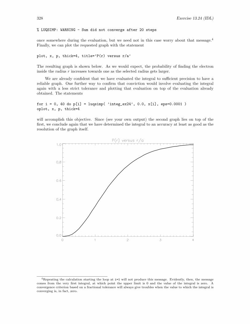
328 Exercise 13.24 (IDL)
% LUQSIMP: WARNING - Sum did not converge after 20 steps
once somewhere during the evaluation, but we need not in this case worry about that message.4
Finally, we can plot the requested graph with the statement
plot, x, p, thick=4, title=’P(r) versus r/a’
The resulting graph is shown below. As we would expect, the probability of finding the electroninside the radius r increases towards one as the selected radius gets larger.
We are already confident that we have evaluated the integral to sufficient precision to have areliable graph. One further way to confirm that conviction would involve evaluating the integralagain with a less strict tolerance and plotting that evaluation on top of the evaluation alreadyobtained. The statements
for i = 0, 40 do p[i] = luqsimp( ’integ_ex24’, 0.0, x[i], eps=0.0001 )
oplot, x, p, thick=4
will accomplish this objective. Since (see your own output) the second graph lies on top of thefirst, we conclude again that we have determined the integral to an accuracy at least as good as theresolution of the graph itself.
4Repeating the calculation starting the loop at i=1 will not produce this message. Evidently, then, the messagecomes from the very first integral, at which point the upper limit is 0 and the value of the integral is zero. Aconvergence criterion based on a fractional tolerance will always give troubles when the value to which the integral isconverging is, in fact, zero.
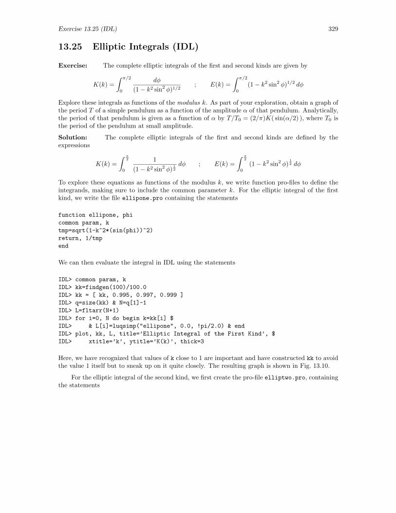
Exercise 13.25 (IDL) 329
13.25 Elliptic Integrals (IDL)
Exercise: The complete elliptic integrals of the first and second kinds are given by
K(k) =
∫ π/2
0
dφ
(1− k2 sin2 φ)1/2; E(k) =
∫ π/2
0
(1− k2 sin2 φ)1/2 dφ
Explore these integrals as functions of the modulus k. As part of your exploration, obtain a graph ofthe period T of a simple pendulum as a function of the amplitude α of that pendulum. Analytically,the period of that pendulum is given as a function of α by T/T0 = (2/π)K( sin(α/2) ), where T0 isthe period of the pendulum at small amplitude.
Solution: The complete elliptic integrals of the first and second kinds are defined by theexpressions
K(k) =
∫ π2
0
1
(1− k2 sin2 φ)12
dφ ; E(k) =
∫ π2
0
(1− k2 sin2 φ)12 dφ
To explore these equations as functions of the modulus k, we write function pro-files to define theintegrands, making sure to include the common parameter k. For the elliptic integral of the firstkind, we write the file ellipone.pro containing the statements
function ellipone, phi
common param, k
tmp=sqrt(1-k^2*(sin(phi))^2)
return, 1/tmp
end
We can then evaluate the integral in IDL using the statements
IDL> common param, k
IDL> kk=findgen(100)/100.0
IDL> kk = [ kk, 0.995, 0.997, 0.999 ]
IDL> q=size(kk) & N=q[1]-1
IDL> L=fltarr(N+1)
IDL> for i=0, N do begin k=kk[i] $
IDL> & L[i]=luqsimp("ellipone", 0.0, !pi/2.0) & end
IDL> plot, kk, L, title=’Elliptic Integral of the First Kind’, $
IDL> xtitle=’k’, ytitle=’K(k)’, thick=3
Here, we have recognized that values of k close to 1 are important and have constructed kk to avoidthe value 1 itself but to sneak up on it quite closely. The resulting graph is shown in Fig. 13.10.
For the elliptic integral of the second kind, we first create the pro-file elliptwo.pro, containingthe statements
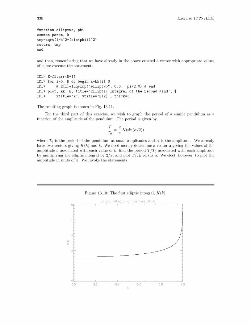
330 Exercise 13.25 (IDL)
function elliptwo, phi
common param, k
tmp=sqrt(1-k^2*(sin(phi))^2)
return, tmp
end
and then, remembering that we have already in the above created a vector with appropriate valuesof k, we execute the statements
IDL> E=fltarr(N+1)
IDL> for i=0, N do begin k=kk[i] $
IDL> & E[i]=luqsimp("elliptwo", 0.0, !pi/2.0) & end
IDL> plot, kk, E, title=’Elliptic Integral of the Second Kind’, $
IDL> xtitle=’k’, ytitle=’E(k)’, thick=3
The resulting graph is shown in Fig. 13.11.
For the third part of this exercise, we wish to graph the period of a simple pendulum as afunction of the amplitude of the pendulum. The period is given by
T
T0=
2
πK(sin(α/2))
where T0 is the period of the pendulum at small amplitudes and α is the amplitude. We alreadyhave two vectors giving K(k) and k. We need merely determine a vector a giving the values of theamplitude a associated with each value of k, find the period T/T0 associated with each amplitudeby multiplying the elliptic integral by 2/π, and plot T/T0 versus a. We elect, however, to plot theamplitude in units of π. We invoke the statements
Figure 13.10: The first elliptic integral, K(k).
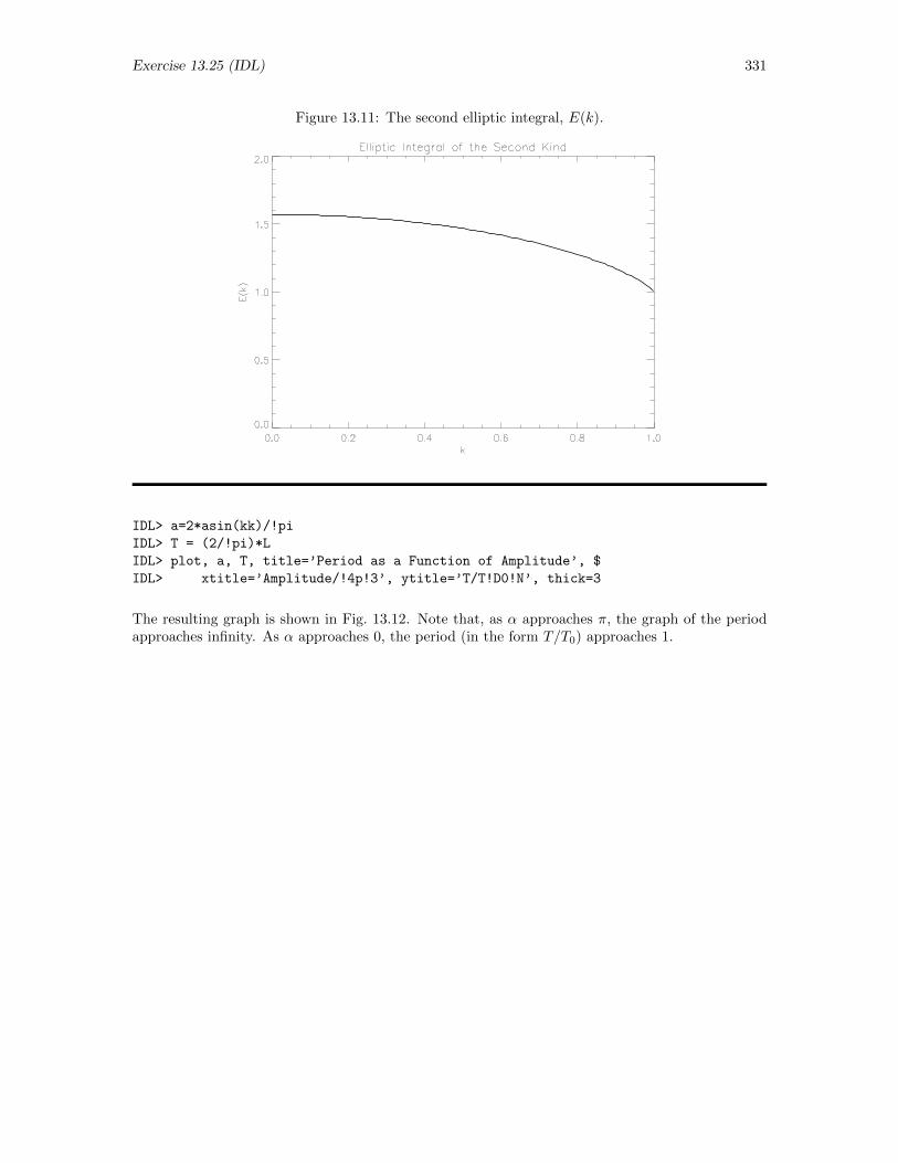
Exercise 13.25 (IDL) 331
Figure 13.11: The second elliptic integral, E(k).
IDL> a=2*asin(kk)/!pi
IDL> T = (2/!pi)*L
IDL> plot, a, T, title=’Period as a Function of Amplitude’, $
IDL> xtitle=’Amplitude/!4p!3’, ytitle=’T/T!D0!N’, thick=3
The resulting graph is shown in Fig. 13.12. Note that, as α approaches π, the graph of the periodapproaches infinity. As α approaches 0, the period (in the form T/T0) approaches 1.
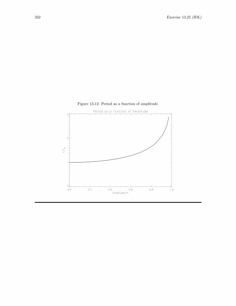
332 Exercise 13.25 (IDL)
Figure 13.12: Period as a function of amplitude.
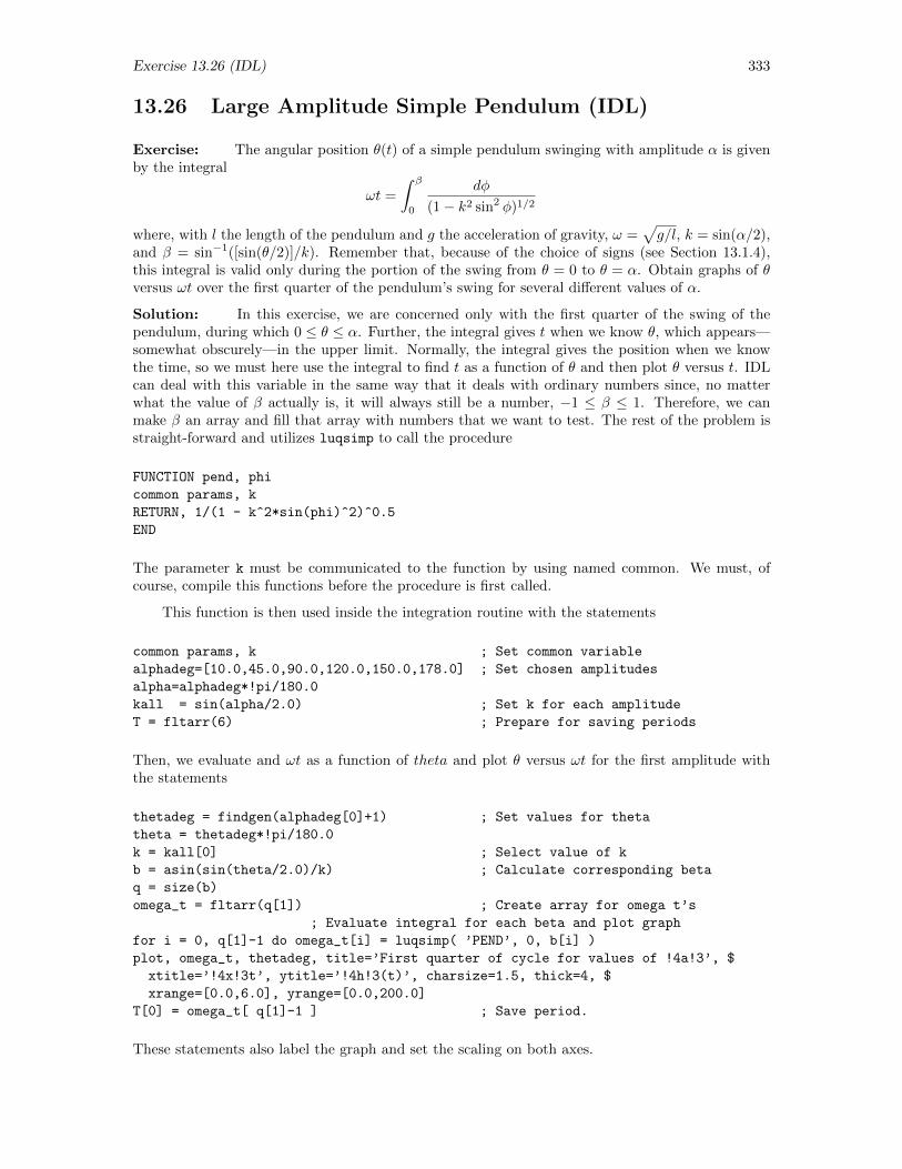
Exercise 13.26 (IDL) 333
13.26 Large Amplitude Simple Pendulum (IDL)
Exercise: The angular position θ(t) of a simple pendulum swinging with amplitude α is givenby the integral
ωt =
∫ β
0
dφ
(1− k2 sin2 φ)1/2
where, with l the length of the pendulum and g the acceleration of gravity, ω =√g/l, k = sin(α/2),
and β = sin−1([sin(θ/2)]/k). Remember that, because of the choice of signs (see Section 13.1.4),this integral is valid only during the portion of the swing from θ = 0 to θ = α. Obtain graphs of θversus ωt over the first quarter of the pendulum’s swing for several different values of α.
Solution: In this exercise, we are concerned only with the first quarter of the swing of thependulum, during which 0 ≤ θ ≤ α. Further, the integral gives t when we know θ, which appears—somewhat obscurely—in the upper limit. Normally, the integral gives the position when we knowthe time, so we must here use the integral to find t as a function of θ and then plot θ versus t. IDLcan deal with this variable in the same way that it deals with ordinary numbers since, no matterwhat the value of β actually is, it will always still be a number, −1 ≤ β ≤ 1. Therefore, we canmake β an array and fill that array with numbers that we want to test. The rest of the problem isstraight-forward and utilizes luqsimp to call the procedure
FUNCTION pend, phi
common params, k
RETURN, 1/(1 - k^2*sin(phi)^2)^0.5
END
The parameter k must be communicated to the function by using named common. We must, ofcourse, compile this functions before the procedure is first called.
This function is then used inside the integration routine with the statements
common params, k ; Set common variable
alphadeg=[10.0,45.0,90.0,120.0,150.0,178.0] ; Set chosen amplitudes
alpha=alphadeg*!pi/180.0
kall = sin(alpha/2.0) ; Set k for each amplitude
T = fltarr(6) ; Prepare for saving periods
Then, we evaluate and ωt as a function of theta and plot θ versus ωt for the first amplitude withthe statements
thetadeg = findgen(alphadeg[0]+1) ; Set values for theta
theta = thetadeg*!pi/180.0
k = kall[0] ; Select value of k
b = asin(sin(theta/2.0)/k) ; Calculate corresponding beta
q = size(b)
omega_t = fltarr(q[1]) ; Create array for omega t’s
; Evaluate integral for each beta and plot graph
for i = 0, q[1]-1 do omega_t[i] = luqsimp( ’PEND’, 0, b[i] )
plot, omega_t, thetadeg, title=’First quarter of cycle for values of !4a!3’, $
xtitle=’!4x!3t’, ytitle=’!4h!3(t)’, charsize=1.5, thick=4, $
xrange=[0.0,6.0], yrange=[0.0,200.0]
T[0] = omega_t[ q[1]-1 ] ; Save period.
These statements also label the graph and set the scaling on both axes.
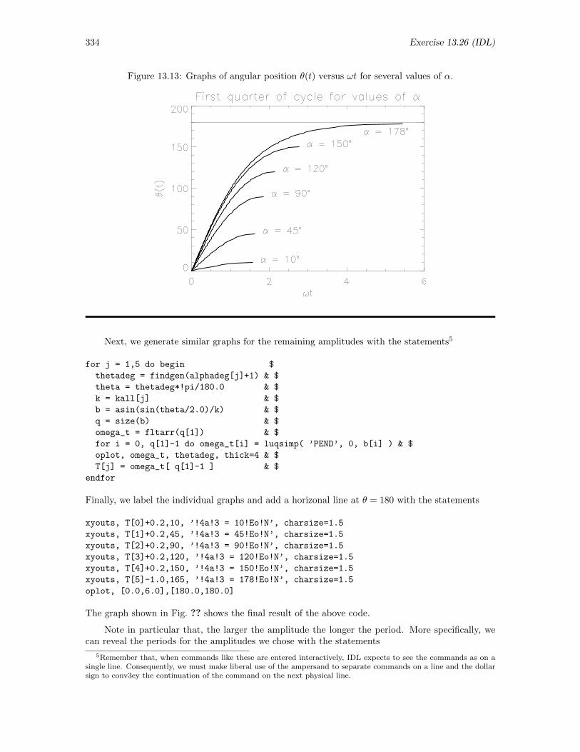
334 Exercise 13.26 (IDL)
Figure 13.13: Graphs of angular position θ(t) versus ωt for several values of α.
Next, we generate similar graphs for the remaining amplitudes with the statements5
for j = 1,5 do begin $
thetadeg = findgen(alphadeg[j]+1) & $
theta = thetadeg*!pi/180.0 & $
k = kall[j] & $
b = asin(sin(theta/2.0)/k) & $
q = size(b) & $
omega_t = fltarr(q[1]) & $
for i = 0, q[1]-1 do omega_t[i] = luqsimp( ’PEND’, 0, b[i] ) & $
oplot, omega_t, thetadeg, thick=4 & $
T[j] = omega_t[ q[1]-1 ] & $
endfor
Finally, we label the individual graphs and add a horizonal line at θ = 180 with the statements
xyouts, T[0]+0.2,10, ’!4a!3 = 10!Eo!N’, charsize=1.5
xyouts, T[1]+0.2,45, ’!4a!3 = 45!Eo!N’, charsize=1.5
xyouts, T[2]+0.2,90, ’!4a!3 = 90!Eo!N’, charsize=1.5
xyouts, T[3]+0.2,120, ’!4a!3 = 120!Eo!N’, charsize=1.5
xyouts, T[4]+0.2,150, ’!4a!3 = 150!Eo!N’, charsize=1.5
xyouts, T[5]-1.0,165, ’!4a!3 = 178!Eo!N’, charsize=1.5
oplot, [0.0,6.0],[180.0,180.0]
The graph shown in Fig. ?? shows the final result of the above code.
Note in particular that, the larger the amplitude the longer the period. More specifically, wecan reveal the periods for the amplitudes we chose with the statements
5Remember that, when commands like these are entered interactively, IDL expects to see the commands as on asingle line. Consequently, we must make liberal use of the ampersand to separate commands on a line and the dollarsign to conv3ey the continuation of the command on the next physical line.
Exercise 13.26 (IDL) 335
T = 4.0*T ; Evaluate actual period
alphadeg
10.000000 45.000000 90.000000 120.00000 150.00000 178.00000
T
6.2951689 6.5343456 7.4162989 8.6260633 11.072254 21.739559
For small amplitude, both α and θ approach zero, so the ratio approaches 1 and β = sin−1(1) = π/2and
ωt =
∫ π/2
0
dφ =π
2
so 4ωt = 2π and the small amplitude period in the units used above is 2π = 6.2832. Thus, relativeto the small amplitude period,
T = T/6.2832 ; Calculate relative periods
alphadeg
10.000000 45.000000 90.000000 120.00000 150.00000 178.00000
T
1.0019050 1.0399710 1.1803379 1.3728775 1.7621999 3.4599504
Even at 45 the small angle approximation to the period of a real pendulum is off by only 4%!
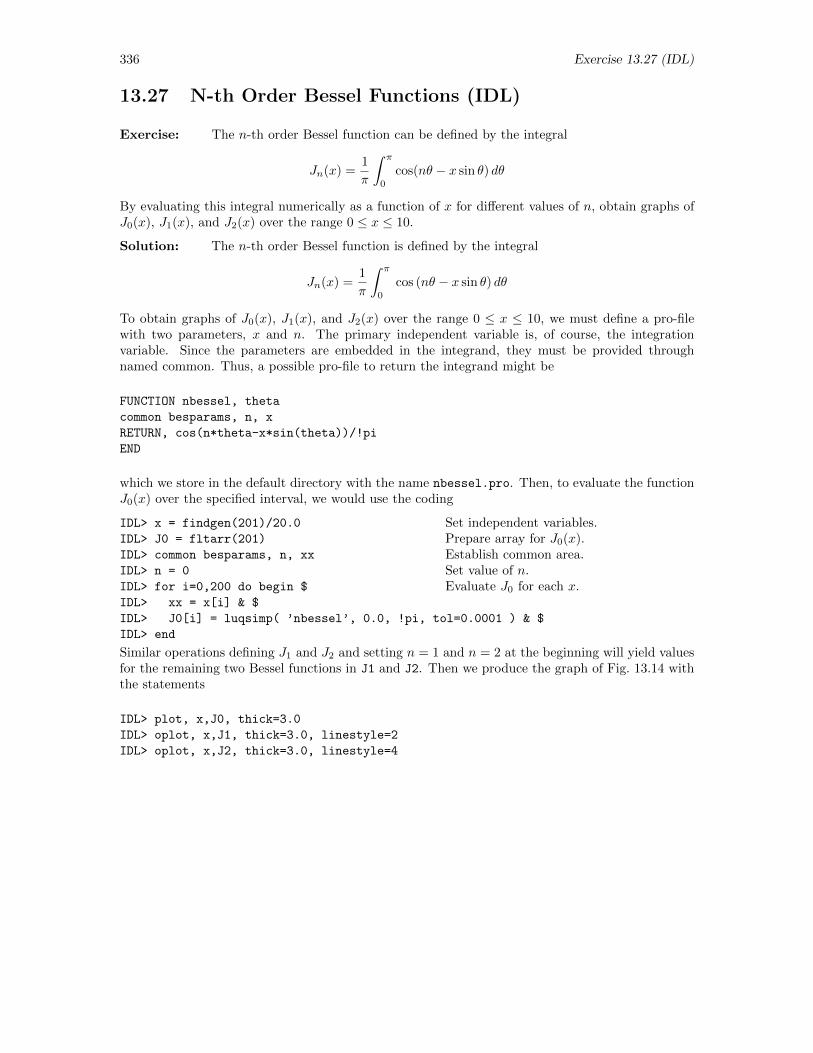
336 Exercise 13.27 (IDL)
13.27 N-th Order Bessel Functions (IDL)
Exercise: The n-th order Bessel function can be defined by the integral
Jn(x) =1
π
∫ π
0
cos(nθ − x sin θ) dθ
By evaluating this integral numerically as a function of x for different values of n, obtain graphs ofJ0(x), J1(x), and J2(x) over the range 0 ≤ x ≤ 10.
Solution: The n-th order Bessel function is defined by the integral
Jn(x) =1
π
∫ π
0
cos (nθ − x sin θ) dθ
To obtain graphs of J0(x), J1(x), and J2(x) over the range 0 ≤ x ≤ 10, we must define a pro-filewith two parameters, x and n. The primary independent variable is, of course, the integrationvariable. Since the parameters are embedded in the integrand, they must be provided throughnamed common. Thus, a possible pro-file to return the integrand might be
FUNCTION nbessel, theta
common besparams, n, x
RETURN, cos(n*theta-x*sin(theta))/!pi
END
which we store in the default directory with the name nbessel.pro. Then, to evaluate the functionJ0(x) over the specified interval, we would use the coding
IDL> x = findgen(201)/20.0
IDL> J0 = fltarr(201)
IDL> common besparams, n, xx
IDL> n = 0
IDL> for i=0,200 do begin $
IDL> xx = x[i] & $
IDL> J0[i] = luqsimp( ’nbessel’, 0.0, !pi, tol=0.0001 ) & $
IDL> end
Set independent variables.Prepare array for J0(x).Establish common area.Set value of n.Evaluate J0 for each x.
Similar operations defining J1 and J2 and setting n = 1 and n = 2 at the beginning will yield valuesfor the remaining two Bessel functions in J1 and J2. Then we produce the graph of Fig. 13.14 withthe statements
IDL> plot, x,J0, thick=3.0
IDL> oplot, x,J1, thick=3.0, linestyle=2
IDL> oplot, x,J2, thick=3.0, linestyle=4
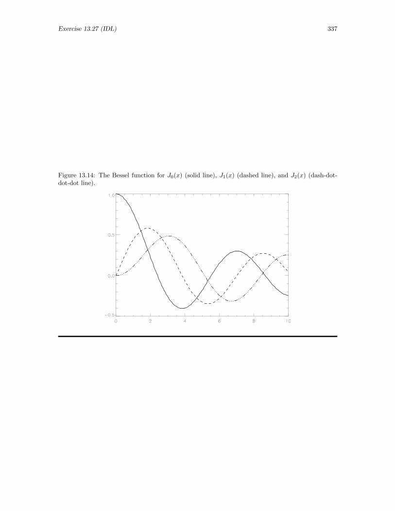
Exercise 13.27 (IDL) 337
Figure 13.14: The Bessel function for J0(x) (solid line), J1(x) (dashed line), and J2(x) (dash-dot-dot-dot line).
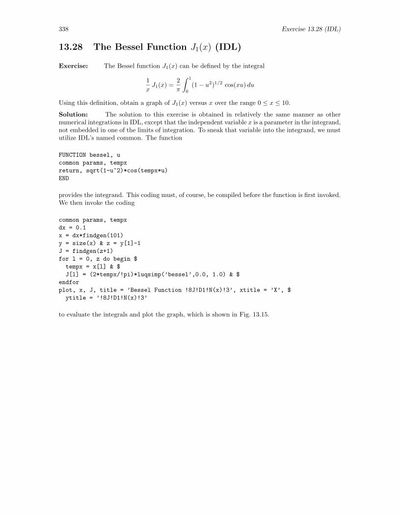
338 Exercise 13.28 (IDL)
13.28 The Bessel Function J1(x) (IDL)
Exercise: The Bessel function J1(x) can be defined by the integral
1
xJ1(x) =
2
π
∫ 1
0
(1− u2)1/2 cos(xu) du
Using this definition, obtain a graph of J1(x) versus x over the range 0 ≤ x ≤ 10.
Solution: The solution to this exercise is obtained in relatively the same manner as othernumerical integrations in IDL, except that the independent variable x is a parameter in the integrand,not embedded in one of the limits of integration. To sneak that variable into the integrand, we mustutilize IDL’s named common. The function
FUNCTION bessel, u
common params, tempx
return, sqrt(1-u^2)*cos(tempx*u)
END
provides the integrand. This coding must, of course, be compiled before the function is first invoked.We then invoke the coding
common params, tempx
dx = 0.1
x = dx*findgen(101)
y = size(x) & z = y[1]-1
J = findgen(z+1)
for l = 0, z do begin $
tempx = x[l] & $
J[l] = (2*tempx/!pi)*luqsimp(’bessel’,0.0, 1.0) & $
endfor
plot, x, J, title = ’Bessel Function !8J!D1!N(x)!3’, xtitle = ’X’, $
ytitle = ’!8J!D1!N(x)!3’
to evaluate the integrals and plot the graph, which is shown in Fig. 13.15.
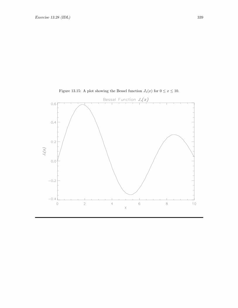
Exercise 13.28 (IDL) 339
Figure 13.15: A plot showing the Bessel function J1(x) for 0 ≤ x ≤ 10.
340 Exercise 13.29 (IDL)
13.29 Off-axis Potential of Circular Ring (IDL)
Exercise: A circular ring of radius a resides in the xy plane with its center at the origin andcarries a charge Q uniformly distributed about its perimeter. The electrostatic potential establishedby this ring at an observation point whose cylindrical coordinates are (r, φ, z) is
V (r, φ, z)
Q/4πε0a=
1
π
∫ π
0
(1− 2
r
acosφ′ +
r2
a2+z2
a2
)−1/2
dφ′
Explore this integral as a function of r/a for several values of z/a.
Solution: A circular ring, radius a, lies in the xy plane with its center at the origin. It carries atotal charge Q uniformly distributed around its circumference, thereby producing an electric field andan electrostatic potential in its vicinity. The electrostatic potential at the point (r, φ, z) (cylindricalcoordinates) is given by the equation
V (r, φ, z)
Q/4πε0a=
1
π
∫ π
0
(1− 2
r
acosφ′ +
r2
a2+z2
a2
)−1/2
dφ′
Introducing the dimensionless quantities R = r/a and Z = z/a, we can simplify this expression to
V (r, φ, z)
Q/4πε0a=
1
π
∫ π
0
(1− 2R cosφ′ +R2 + Z2
)−1/2dφ′
We want to use IDL to explore this electrostatic potential as a function of R for various values ofZ. Choosing to measure V in units of V0 = Q/4πε0a and using the IDL variables r and z for thedimensionless variables R and Z, we first create the function pro-file
function chgdring, phi
;
; Computes the integrand for evaluating the electrostatic
; potential of a charged ring
;
common param, r, z
den= sqrt( 1 - 2*r*cos(phi) + r^2 + z^2 )
return, 1.0/(den*!pi)
end
The parameters r and z, which appear embedded within the integrand, are provided through thenamed common area param.
After storing the above file with the name chdring.pro in the default directory, we are readyto invoke luqsimp to evaluate the integral. We would, for example, determine and plot the x and zcomponents of the field at z = 0.1 with the statements
IDL> common param, rr, zz
IDL> r=findgen(121)/40.0
IDL> q=size(r) & N=q[1]-1
IDL> V01=fltarr(N+1)
IDL> zz=0.1
IDL> for i=0, N do begin rr= r[i] $
IDL> & V01[i]=luqsimp(’chgdring’, 0.0, !pi) & end
IDL> plot,r,V01
Exercise 13.29 (IDL) 341
(It took a bit of experimenting to find a suitable range of values over which to extend the variabler.) The results are incorporated in the more complete graph in Fig. 13.16.
Similar statements generate the magnetic fields for other values of z. In particular, we executethe statements
IDL> V03=fltarr(N+1)
IDL> zz=0.3
IDL> for i=0, N do begin rr= r[i] $
IDL> & V03[i]=luqsimp(’chgdring’, 0.0, !pi) & end
IDL> V06=fltarr(N+1)
IDL> zz=0.6
IDL> for i=0, N do begin rr= r[i] $
IDL> & V06[i]=luqsimp(’chgdring’, 0.0, !pi) & end
IDL> V10=fltarr(N+1)
IDL> zz=1.0
IDL> for i=0, N do begin rr= r[i] $
IDL> & V10[i]=luqsimp(’chgdring’, 0.0, !pi) & end
Finally, we generate a composite plot showing the x component of the magnetic field producedby this source by invoking the statements
IDL> plot, r, V01, title=’Electrostatic Potential of Charged Ring’, $
IDL> xtitle=’r/a’, ytitle=’V/V_0’, linestyle=4, thick=3
IDL> oplot, r, V03, linestyle=2, thick=3
IDL> oplot, r, V06, linestyle=3, thick=3
IDL> oplot, r, V10, linestyle=1, thick=3
IDL> plots, [1.5, 2.1], [1.4, 1.4], linestyle=4, thick=3
IDL> xyouts, 2.2, 1.4, ’z/a=0.1’
IDL> plots, [1.5, 2.1], [1.3, 1.3], linestyle=2, thick=3
IDL> xyouts, 2.2, 1.3, ’z/a=0.3’
IDL> plots, [1.5, 2.1], [1.2, 1.2], linestyle=3, thick=3
IDL> xyouts, 2.2, 1.2, ’z/a=0.6’
IDL> plots, [1.5, 2.1], [1.1, 1.1], linestyle=1, thick=3
IDL> xyouts, 2.2, 1.1, ’z/a=1.0’
The resulting graph is shown in 13.16. Note that, since x/a = 1 corresponds to the point directlyabove the loop, the peaks in these graphs occur right over the loop.
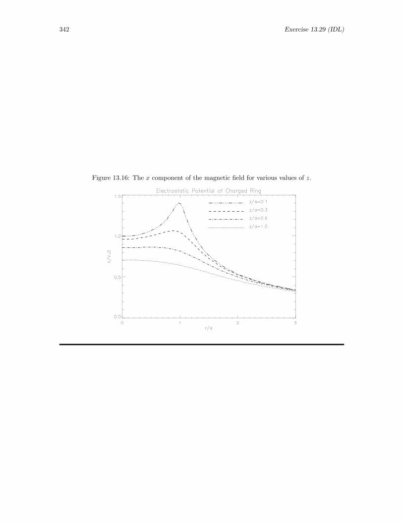
342 Exercise 13.29 (IDL)
Figure 13.16: The x component of the magnetic field for various values of z.
Exercise 13.30 (IDL) 343
13.30 Off-axis Field of Current Loop (IDL)
Exercise: A circular current loop of radius a lies in the xy-plane with its center at the originand carries a current I ′ counterclockwise as viewed from a point on the positive z axis. The magneticfield at a point in the xz plane is given by
B(x, z)
µ0I ′/2πa= a2
∫ π
0
z cosφ′ i + (a− x cosφ′) k
[x2 + z2 + a2 − 2ax cosφ′]3/2dφ′
Explore both components of this magnetic field numerically as functions of x/a for various valuesof z/a, including z/a = 0.0 (which will require some creativity for dealing with the point x/a = 1.0,at which the integrand diverges at one point in the range of the integration variable).
Solution: A circular current loop, radius a, lies in the xy plane with its center at the origin.It carries a current I ′ counterclockwise as viewed from the positive z axis, thereby producing amagnetic field B. This field, at a point in the xz plane, is given by the equation
B(x, z)
µoI ′/2πa= a2
∫ π
0
z cosφ′ i + (a− x cosφ′)k
[x2 + z2 + a2 − 2ax cosφ′]3/2dφ′
Introducing the dimensionless quantities X = x/a and Z = z/a, we can simplify this expression to
B(X,Z)
µoI ′/2πa=
∫ π
0
Z cosφ′ i + (1−X cosφ′)k
[X2 + Z2 + 1− 2X cosφ′]3/2dφ′
We want to use IDL to explore both components of this field as functions of X for various values ofZ. Choosing to measure B in units of B0 = µ0I
′/2πa and using the IDL variables x and z for thedimensionless variables X and Z, we first create the function pro-files
function magneticx, phi
;
; Computes the integrand for evaluating the x component
; of the B field of a circular current loop
;
common param, x, z
den= (x^2 + z^2 +1-2*x*cos(phi))^1.5
return, z*cos(phi)/den
end
and
function magneticz, phi
;
; Computes the integrand for evaluating the z component
; of the B field of a circular current loop
;
common param, x, z
den= (x^2 + z^2 +1-2*x*cos(phi))^1.5
return, (1-x*cos(phi))/den
end
In each case, the parameters x and z, which appear embedded within the integrands, are providedthrough the named common area param. These functions, of course, return the x and z componentsof the integrand, respectively.
Now, we are ready to invoke luqsimp to evaluate the integrals. We would, for example, deter-mine and plot the x and z components of the field at z = 0.1 with the statements
344 Exercise 13.30 (IDL)
IDL> common param, xx, zz
IDL> x=findgen(121)/40.0
IDL> q=size(x) & N=q[1]-1
IDL> Bx01=fltarr(N+1) & Bz01=fltarr(N+1)
IDL> zz=0.1
IDL> for i=0, N do begin xx= x[i] $
IDL> & Bx01[i]=luqsimp(’magneticx’, 0.0, !pi) $
IDL> & Bz01[i]=luqsimp(’magneticz’, 0.0, !pi ) & end
IDL> !p.multi=[0,1,2]
IDL> plot,x,Bx01,xtitle=’x’,ytitle=’B_x’,thick=3
IDL> plot,x,Bz01,xtitle=’x’,ytitle=’B_z’,thick=3
(It took a bit of experimenting to find a suitable range of values over which to extend the variablex.) The results are incorporated in the more complete graphs of Figs. 13.17 and 13.18
Similar statements generate the magnetic fields for other values of z. In particular, we executethe statements
IDL> Bx03=fltarr(N+1) & Bz03=fltarr(N+1)
IDL> zz=0.3
IDL> for i=0, N do begin xx= x[i] $
IDL> & Bx03[i]=luqsimp(’magneticx’, 0.0, !pi) $
IDL> & Bz03[i]=luqsimp(’magneticz’, 0.0, !pi ) & end
IDL> Bx06=fltarr(N+1) & Bz06=fltarr(N+1)
IDL> zz=0.6
IDL> for i=0, N do begin xx= x[i] $
IDL> & Bx06[i]=luqsimp(’magneticx’, 0.0, !pi) $
IDL> & Bz06[i]=luqsimp(’magneticz’, 0.0, !pi ) & end
IDL> Bx10=fltarr(N+1) & Bz10=fltarr(N+1)
IDL> zz=1.0
IDL> for i=0, N do begin xx= x[i] $
IDL> & Bx10[i]=luqsimp(’magneticx’, 0.0, !pi) $
IDL> & Bz10[i]=luqsimp(’magneticz’, 0.0, !pi ) & end
Finally, we generate a composite plot showing the x component of the magnetic field producedby this source by invoking the statements
IDL> !p.multi=0
IDL> plot, x, Bx01, title=’x Component of Magnetic Field’, xtitle=’x/a’,$
IDL> ytitle=’B_x/B_0’, xrange=[0.0, 3.0], linestyle=4, thick=3
IDL> oplot, x, Bx03, linestyle=2, thick=3
IDL> oplot, x, Bx06, linestyle=3, thick=3
IDL> oplot, x, Bx10, linestyle=1, thick=3
IDL> plots, [1.5, 2.1], [9.0, 9.0], linestyle=4, thick=3
IDL> xyouts, 2.2, 9.0, ’z/a=0.1’
IDL> plots, [1.5, 2.1], [8.0, 8.0], linestyle=2, thick=3
IDL> xyouts, 2.2, 8.0, ’z/a=0.3’
IDL> plots, [1.5, 2.1], [7.0, 7.0], linestyle=3, thick=3
IDL> xyouts, 2.2, 7.0, ’z/a=0.6’
IDL> plots, [1.5, 2.1], [6.0, 6.0], linestyle=1, thick=3
IDL> xyouts, 2.2, 6.0, ’z/a=1.0’
The resulting graph is shown in Fig. 13.17. Note that, since x/a = 1 corresponds to the pointdirectly above the loop, the peaks in these graphs occur right over the loop.
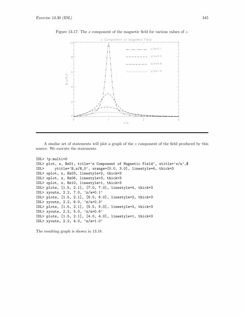
Exercise 13.30 (IDL) 345
Figure 13.17: The x component of the magnetic field for various values of z.
A similar set of statements will plot a graph of the z component of the field produced by thissource. We execute the statements
IDL> !p.multi=0
IDL> plot, x, Bz01, title=’z Component of Magnetic Field’, xtitle=’x/a’,$
IDL> ytitle=’B_z/B_0’, xrange=[0.0, 3.0], linestyle=4, thick=3
IDL> oplot, x, Bz03, linestyle=2, thick=3
IDL> oplot, x, Bz06, linestyle=3, thick=3
IDL> oplot, x, Bz10, linestyle=1, thick=3
IDL> plots, [1.5, 2.1], [7.0, 7.0], linestyle=4, thick=3
IDL> xyouts, 2.2, 7.0, ’z/a=0.1’
IDL> plots, [1.5, 2.1], [6.0, 6.0], linestyle=2, thick=3
IDL> xyouts, 2.2, 6.0, ’z/a=0.3’
IDL> plots, [1.5, 2.1], [5.0, 5.0], linestyle=3, thick=3
IDL> xyouts, 2.2, 5.0, ’z/a=0.6’
IDL> plots, [1.5, 2.1], [4.0, 4.0], linestyle=1, thick=3
IDL> xyouts, 2.2, 4.0, ’z/a=1.0’
The resulting graph is shown in 13.18.
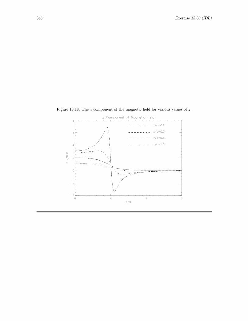
346 Exercise 13.30 (IDL)
Figure 13.18: The z component of the magnetic field for various values of z.
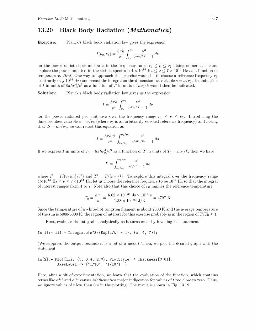
Exercise 13.20 Mathematica) 347
13.20 Black Body Radiation (Mathematica)
Exercise: Planck’s black body radiation law gives the expression
I(ν2, ν1) =8πh
c3
∫ ν2
ν1
ν3
ehν/kT − 1dν
for the power radiated per unit area in the frequency range ν1 ≤ ν ≤ ν2. Using numerical means,explore the power radiated in the visible spectrum 4× 10¹⁴ Hz ≤ ν ≤ 7× 10¹⁴ Hz as a function oftemperature. Hint : One way to approach this exercise would be to choose a reference frequency ν0
arbitrarily (say 1014 Hz) and recast the integral on the dimensionless variable s = ν/ν0. Examinationof I in units of 8πhν4
0/c3 as a function of T in units of hν0/k would then be indicated.
Solution: Planck’s black body radiation law gives us the expression
I =8πh
c3
∫ ν2
ν1
ν3
ehv/kT − 1dν
for the power radiated per unit area over the frequency range ν1 ≤ ν ≤ ν2. Introducing thedimensionless variable s = ν/ν0 (where ν0 is an arbitrarily selected reference frequency) and notingthat ds = dν/ν0, we can recast this equation as
I =8πhν4
0
c3
∫ ν2/ν0
ν1/ν0
s3
ehsν0/kT − 1ds
If we express I in units of I0 = 8πhν40/c
3 as a function of T in units of T0 = hν0/k, then we have
I ′ =
∫ ν2/ν0
ν1/ν0
s3
es/T ′ − 1ds
where I ′ = I/(8πhν40/c
3) and T ′ = T/(hν0/k). To explore this integral over the frequency range4×1014 Hz ≤ ν ≤ 7×10¹⁴ Hz, let us choose the reference frequency to be 1014 Hz so that the integralof interest ranges from 4 to 7. Note also that this choice of ν0 implies the reference temperature
T0 =hν0
k=
6.62× 10−34 Js× 1014 s
1.38× 10⁻²³ J/K= 4797 K
Since the temperature of a white-hot tungsten filament is about 2800 K and the average temperatureof the sun is 5000-6000 K, the region of interest for this exercise probably is in the region of T/T0 ≤ 1.
First, evaluate the integral—analytically as it turns out—by invoking the statement
In[1]:= iii = Integrate[s^3/(Exp[s/t] - 1), s, 4, 7];
(We suppress the output because it is a bit of a mess.) Then, we plot the desired graph with thestatement
In[2]:= Plot[iii, t, 0.4, 2.0, PlotStyle -> Thickness[0.01],
AxesLabel -> "T/T0", "I/I0" ]
Here, after a bit of experimentation, we learn that the evaluation of the function, which containsterms like e4/t and e7/t causes Mathematica major indigestion for values of t too close to zero. Thus,we ignore values of t less than 0.4 in the plotting. The result is shown in Fig. 13.19.
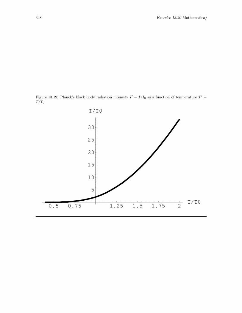
348 Exercise 13.20 Mathematica)
Figure 13.19: Planck’s black body radiation intensity I ′ = I/I0 as a function of temperature T ′ =T/T0.
0.5 0.75 1.25 1.5 1.75 2T/T0
5
10
15
20
25
30
I/I0
Exercise 13.21 (Mathematica) 349
13.21 Confidence Intervals for Gaussian (Mathematica)
Exercise: As used in statistical data analysis, the Gaussian distribution for a variable t isusually expressed in terms of the standard deviation σ, the distribution function being
1√2π σ
e−t2/2σ2
Thus, the probability of finding a value between a and b is given by
P (a, b) =1√2πσ
∫ b
a
e−t2/(2σ2) dt
Show analytically that P (−x, x) = erf(x/(√
2σ)), and then evaluate P (−σ, σ), P (−2σ, 2σ), andP (−3σ, 3σ) numerically. The values of these three quantities are 0.6827, 0.9545, and 0.9973,respectively—values that give rise to the designations of 68%, 95%, and 99% confidence intervals instatistical data analysis.
Solution: The probability that a single measurement drawn from a normally distributed uni-verse of possible values will lie between a and b is given by the integral
P (a, b) =1√2πσ
∫ b
a
e−t2/(2σ2) dt
To show analytically that P (−x, x) = erf(x/(√
2σ)), we simply change variables. If we let t2/2σ2 =s2, then dt =
√2σ ds and, when t = x, s = x/
√2σ. Thus, the integral becomes
P (−x, x) =1√π
∫ x/√
2σ
−x/√
2σ
e−s2
ds =2√π
∫ x/√
2σ
0
e−s2
ds = erf
(x√2σ
)The first equality is a result of the change of variables. The second stems from the observations that(1) the integrand is an even function of the integration variable and (2) the limits are symmetric.
Another way to determine the relationship between P (−x, x) and erf(x) is to integrate theprobability function symbolically. We can define the integrand and perform the integral by enteringthe statements
In[1]:= integrand = Exp[-t^2/(2*\[Sigma]^2)];
In[2]:= coef = 1/(Sqrt[2*Pi]*\[Sigma]);
In[3]:= p = coef * Integrate[integrand, t, -x, x]
Out[3]= Erf(x√2σ
)
This sequence of statements to Mathematica confirms the demonstration of the previous paragraphthat P (−x, x) = erf(x/(
√2σ)).
To evaluate the probability function for particular values of x, it is only necessary to evaluatethe error function for x/(
√2σ). For x = σ, 2σ, and 3σ, respectively, we seek the value of erf(1/
√2),
erf(2/√
2), and erf(3/√
2). Appropriate statements are
In[4]:= N[p /. x -> \[Sigma]]
Out[4]= 0.682689
In[5]:= N[p /. x -> 2*\[Sigma]]
Out[5]= 0.9545
In[6]:= N[p /. x -> 3*\[Sigma]]
Out[6]= 0.9973

350 Exercise 13.21 (Mathematica)
We conclude that a single value randomly selected from a Gaussian distribution stands a 68.3%chance of falling within one standard deviation of the mean, a 95.4% chance of falling within twostandard deviations, and a 99.7% chance of falling within three standard deviations.
Exercise 13.23 (Mathematica) 351
13.23 Properties of Lorentz Distribution (Mathematica)
Exercise: The normalized Lorentz distribution function is given by
p(x) =1
π
a/2
x2 + (a/2)2
Find the probability that a single, randomly selected value will be in the range −a ≤ x ≤ a. Makesure to assess the precision of your result by methods that do not exploit a priori knowledge of theexact value. Hint : Before evaluating the integral, introduce the dimensionless variable s = x/a andnote that the result actually doesn’t depend on a, so there is but one number to determine.
Solution: The normalized Lorentz distribution function is
p(x) =1
π
a/2
x2 + (a/2)2
To find the probability that a random value will be in the range a ≤ x ≤ a, we simply integratep(x)dx from a to −a. First, however, let us subsitute the dimensionless variable s = x/a. Then theintegral we wish to evaluate becomes∫ a
−ap(x) dx =
1
2π
∫ 1
−1
1
s2 + (1/4)ds
We explored this integral symbolically in Exercise 11.5. Here, we wish to exhibit Mathematica’scapabilities to evaluate integrals numerically. To do so, we invoke the statement
In[1]:= p = (1/(2*Pi))/(s^2+1/4)
Out[1]=1
2π(1/4 + s2)
to define the integrand. Then, we evaluate the integral directly by a numerical method with thestatement
In[2]:= NIntegrate[ p, s, -1.0, 1.0 ]
Out[2]= 0.704833
The probability that a value will fall in that range −a ≤ x ≤ a is evidently 70.5%. By default, theoption variable PrecisionGoal has the value 6 (10 less than the working precision of 16), so weshould be able to believe all six digits printed out.
We can obtain a numerical evaluation of the integral to more digits by evaluating the integralanalytically and then converting the result to a numerical value. Statements achieving that objectiveare
In[3]:= N[ Integrate[ p, s, -1, 1], 20 ]
Out[3]= 0.70483276469913345165
(Explicit decimal points in the limits will subvert the request for 20 digits in the output.)
352 Exercise 13.32 (FORTRAN)
13.32 Simpson’s Rule (FORTRAN)
Exercise: Patterning your program after the program trapezoidal.f, write and test a FOR-TRAN program that uses Simpson’s rule to evaluate
I =2√π
∫ b
a
e−x2
dx
Solution: We want to write and test a FORTRAN program that will use Simpson’s rule
I =∆x
3(f0 + 4f1 + 2f2 + · · ·+ 2fn−2 + 4fn−1 + fn)
to evaluate the integral
I =2√π
∫ b
a
e−x2
dx
for limits and number of divisions entered at the time of execution. The program trapezoidal.f canserve as a model for the program to be created. We need, of course, to have a function subprogramto return the value of the integrand. An appropriate segment of the code would then involve thestatements
FUNCTION FUNC(X)
FUNC = 2.0*EXP(-X**2)/SQRT(3.14159265)
END
The limits and number of divisions would be obtained from the keyboard with statements identicalto those in trapezoidal.f, namely
WRITE(*, ’(1X,A)’) ’Lower limit? ’
READ(*,*) A
WRITE(*, ’(1X,A)’) ’Upper limit? ’
READ(*,*) B
WRITE(*, ’(1X,A)’) ’Number of divisions? ’
READ(*,*) N
We would then have to set the increment that expresses the width of each strip in the division ofthe interval a ≤ x ≤ b into n segments with the statement
DX = (B-A)/FLOAT(N) ! Set size of segment
Then, the evaluation of the integral would be achieved by adding up the several terms in the aboveequation. To achieve that end, we would use the statements
VAL = FUNC(A) ! Initialize to first term
DO I=1, N-1, 2 ! Add terms multiplied by 4
VAL = VAL + 4.0*FUNC(A+I*DX)
ENDDO
DO I=2, N-2, 2 ! Add terms multiplied by 2
VAL = VAL + 2.0*FUNC(A+I*DX)
ENDDO
VAL = VAL + FUNC(B) ! Add final term
VAL = VAL*DX/3.0 ! Incorporate overall factor
Finally, we display the value of the integral with the statement
Exercise 13.32 (FORTRAN) 353
WRITE(*, ’(1X,A,F12.6)’) ’Integral = ’, VAL
As a futher wrinkle, however, let us recognize that Simpson’s rule requires n to be even andlet’s build in a routine to reject inadvertently entered odd values of n. We would simply test n asit is entered and return to ask for it again if the entered value happens to be odd. To that end, wewould modify the statements requesting the FORTRAN variable N to have the form
WRITE(*, ’(1X,A)’) ’Number of divisions? ’
READ(*,*) N
DO WHILE (N/2 .NE. FLOAT(N)/2.0)
WRITE(*, ’(1X,A)’) ’Value of N must be even.’
WRITE(*, ’(1X,A)’) ’Number of divisions? ’
READ(*,*) N
ENDDO
The full program (including a few added comments) is listed on a page by itself at the end of thissolution
Once saved in the default directory with the name simpson.f, this program can be compiledand run using the statements
f77 -o simpson.xf simpson.f
./simpson.xf
In response, the “conversation” with the computer might look like6
Lower limit? 0
Upper limit? 1
Number of divisions? 8
Integral = 0.842703
We test the program’s capacity to reject odd values of n with the statements
./simpson.xf
Lower limit? 0
Upper limit? 1
Number of divisions? 15
Value of N must be even.
Number of divisions? 17
Value of N must be even.
Number of divisions? 16
Integral = 0.842701
Finally, we test the convergence of this evaluation by executing similar statements with other valuesof n, obtaining the results
n Integral
2 0.8431034 0.8427368 0.842703
16 0.84270132 0.84270164 0.842701
128 0.842701
6Values input in response to prompts have here been placed on the same line as the prompt to save space.

354 Exercise 13.32 (FORTRAN)
By the time 16 divisions have been used, the value of the integral has converged to 0.842701. Asillustrated in the text, the program trapezoidal.f required on the order of 256 or even 512 divisionsbefore the results it generated had converged to six digits after the decimal place.
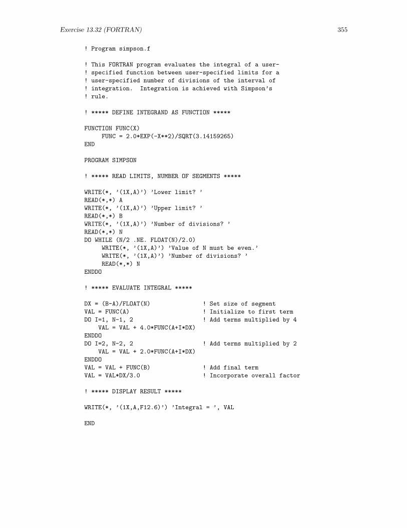
Exercise 13.32 (FORTRAN) 355
! Program simpson.f
! This FORTRAN program evaluates the integral of a user-
! specified function between user-specified limits for a
! user-specified number of divisions of the interval of
! integration. Integration is achieved with Simpson’s
! rule.
! ***** DEFINE INTEGRAND AS FUNCTION *****
FUNCTION FUNC(X)
FUNC = 2.0*EXP(-X**2)/SQRT(3.14159265)
END
PROGRAM SIMPSON
! ***** READ LIMITS, NUMBER OF SEGMENTS *****
WRITE(*, ’(1X,A)’) ’Lower limit? ’
READ(*,*) A
WRITE(*, ’(1X,A)’) ’Upper limit? ’
READ(*,*) B
WRITE(*, ’(1X,A)’) ’Number of divisions? ’
READ(*,*) N
DO WHILE (N/2 .NE. FLOAT(N)/2.0)
WRITE(*, ’(1X,A)’) ’Value of N must be even.’
WRITE(*, ’(1X,A)’) ’Number of divisions? ’
READ(*,*) N
ENDDO
! ***** EVALUATE INTEGRAL *****
DX = (B-A)/FLOAT(N) ! Set size of segment
VAL = FUNC(A) ! Initialize to first term
DO I=1, N-1, 2 ! Add terms multiplied by 4
VAL = VAL + 4.0*FUNC(A+I*DX)
ENDDO
DO I=2, N-2, 2 ! Add terms multiplied by 2
VAL = VAL + 2.0*FUNC(A+I*DX)
ENDDO
VAL = VAL + FUNC(B) ! Add final term
VAL = VAL*DX/3.0 ! Incorporate overall factor
! ***** DISPLAY RESULT *****
WRITE(*, ’(1X,A,F12.6)’) ’Integral = ’, VAL
END
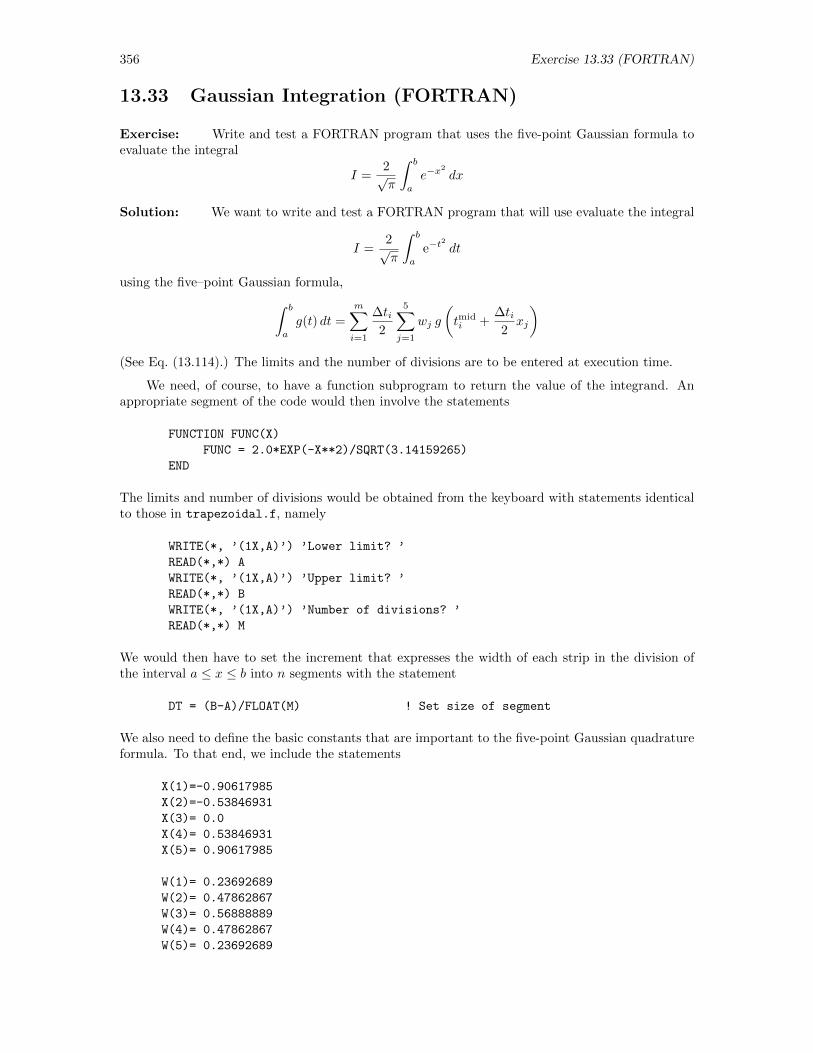
356 Exercise 13.33 (FORTRAN)
13.33 Gaussian Integration (FORTRAN)
Exercise: Write and test a FORTRAN program that uses the five-point Gaussian formula toevaluate the integral
I =2√π
∫ b
a
e−x2
dx
Solution: We want to write and test a FORTRAN program that will use evaluate the integral
I =2√π
∫ b
a
e−t2
dt
using the five–point Gaussian formula,∫ b
a
g(t) dt =
m∑i=1
∆ti2
5∑j=1
wj g
(tmidi +
∆ti2xj
)(See Eq. (13.114).) The limits and the number of divisions are to be entered at execution time.
We need, of course, to have a function subprogram to return the value of the integrand. Anappropriate segment of the code would then involve the statements
FUNCTION FUNC(X)
FUNC = 2.0*EXP(-X**2)/SQRT(3.14159265)
END
The limits and number of divisions would be obtained from the keyboard with statements identicalto those in trapezoidal.f, namely
WRITE(*, ’(1X,A)’) ’Lower limit? ’
READ(*,*) A
WRITE(*, ’(1X,A)’) ’Upper limit? ’
READ(*,*) B
WRITE(*, ’(1X,A)’) ’Number of divisions? ’
READ(*,*) M
We would then have to set the increment that expresses the width of each strip in the division ofthe interval a ≤ x ≤ b into n segments with the statement
DT = (B-A)/FLOAT(M) ! Set size of segment
We also need to define the basic constants that are important to the five-point Gaussian quadratureformula. To that end, we include the statements
X(1)=-0.90617985
X(2)=-0.53846931
X(3)= 0.0
X(4)= 0.53846931
X(5)= 0.90617985
W(1)= 0.23692689
W(2)= 0.47862867
W(3)= 0.56888889
W(4)= 0.47862867
W(5)= 0.23692689
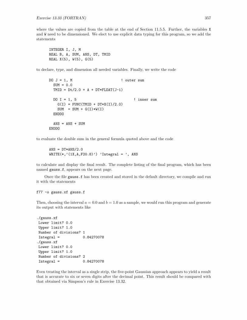
Exercise 13.33 (FORTRAN) 357
where the values are copied from the table at the end of Section 11.5.5. Further, the variables X
and W need to be dimensioned. We elect to use explicit data typing for this program, so we add thestatements
INTEGER I, J, M
REAL B, A, SUM, ANS, DT, TMID
REAL X(5), W(5), G(5)
to declare, type, and dimension all needed variables. Finally, we write the code
DO J = 1, M ! outer sum
SUM = 0.0
TMID = Dt/2.0 + A + DT*FLOAT(J-1)
DO I = 1, 5 ! inner sum
G(I) = FUNC(TMID + DT*X(I)/2.0)
SUM = SUM + G(I)*W(I)
ENDDO
ANS = ANS + SUM
ENDDO
to evaluate the double sum in the general formula quoted above and the code
ANS = DT*ANS/2.0
WRITE(*,’(1X,A,F20.8)’) ’Integral = ’, ANS
to calculate and display the final result. The complete listing of the final program, which has beennamed gauss.f, appears on the next page.
Once the file gauss.f has been created and stored in the default directory, we compile and runit with the statements
f77 -o gauss.xf gauss.f
Then, choosing the interval a = 0.0 and b = 1.0 as a sample, we would run this program and generateits output with statements like
./gauss.xf
Lower limit? 0.0
Upper limit? 1.0
Number of divisions? 1
Integral = 0.84270078
./gauss.xf
Lower limit? 0.0
Upper limit? 1.0
Number of divisions? 2
Integral = 0.84270078
Even treating the interval as a single strip, the five-point Gaussian approach appears to yield a resultthat is accurate to six or seven digits after the decimal point. This result should be compared withthat obtained via Simpson’s rule in Exercise 13.32.
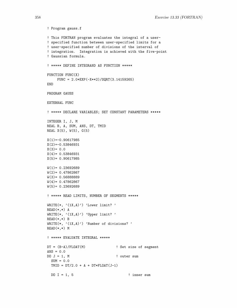
358 Exercise 13.33 (FORTRAN)
! Program gauss.f
! This FORTRAN program evaluates the integral of a user-
! specified function between user-specified limits for a
! user-specified number of divisions of the interval of
! integration. Integration is achieved with the five-point
! Gaussian formula.
! ***** DEFINE INTEGRAND AS FUNCTION *****
FUNCTION FUNC(X)
FUNC = 2.0*EXP(-X**2)/SQRT(3.14159265)
END
PROGRAM GAUSS
EXTERNAL FUNC
! ***** DECLARE VARIABLES; SET CONSTANT PARAMETERS *****
INTEGER I, J, M
REAL B, A, SUM, ANS, DT, TMID
REAL X(5), W(5), G(5)
X(1)=-0.90617985
X(2)=-0.53846931
X(3)= 0.0
X(4)= 0.53846931
X(5)= 0.90617985
W(1)= 0.23692689
W(2)= 0.47862867
W(3)= 0.56888889
W(4)= 0.47862867
W(5)= 0.23692689
! ***** READ LIMITS, NUMBER OF SEGMENTS *****
WRITE(*, ’(1X,A)’) ’Lower limit? ’
READ(*,*) A
WRITE(*, ’(1X,A)’) ’Upper limit? ’
READ(*,*) B
WRITE(*, ’(1X,A)’) ’Number of divisions? ’
READ(*,*) M
! ***** EVALUATE INTEGRAL *****
DT = (B-A)/FLOAT(M) ! Set size of segment
ANS = 0.0
DO J = 1, M ! outer sum
SUM = 0.0
TMID = DT/2.0 + A + DT*FLOAT(J-1)
DO I = 1, 5 ! inner sum

Exercise 13.33 (FORTRAN) 359
G(I) = FUNC(TMID + DT*X(I)/2.0)
SUM = SUM + G(I)*W(I)
ENDDO
ANS = ANS + SUM
ENDDO
ANS = DT*ANS/2.0
! ***** DISPLAY RESULT *****
WRITE(*,’(1X,A,F20.8)’) ’Integral = ’, ANS
END
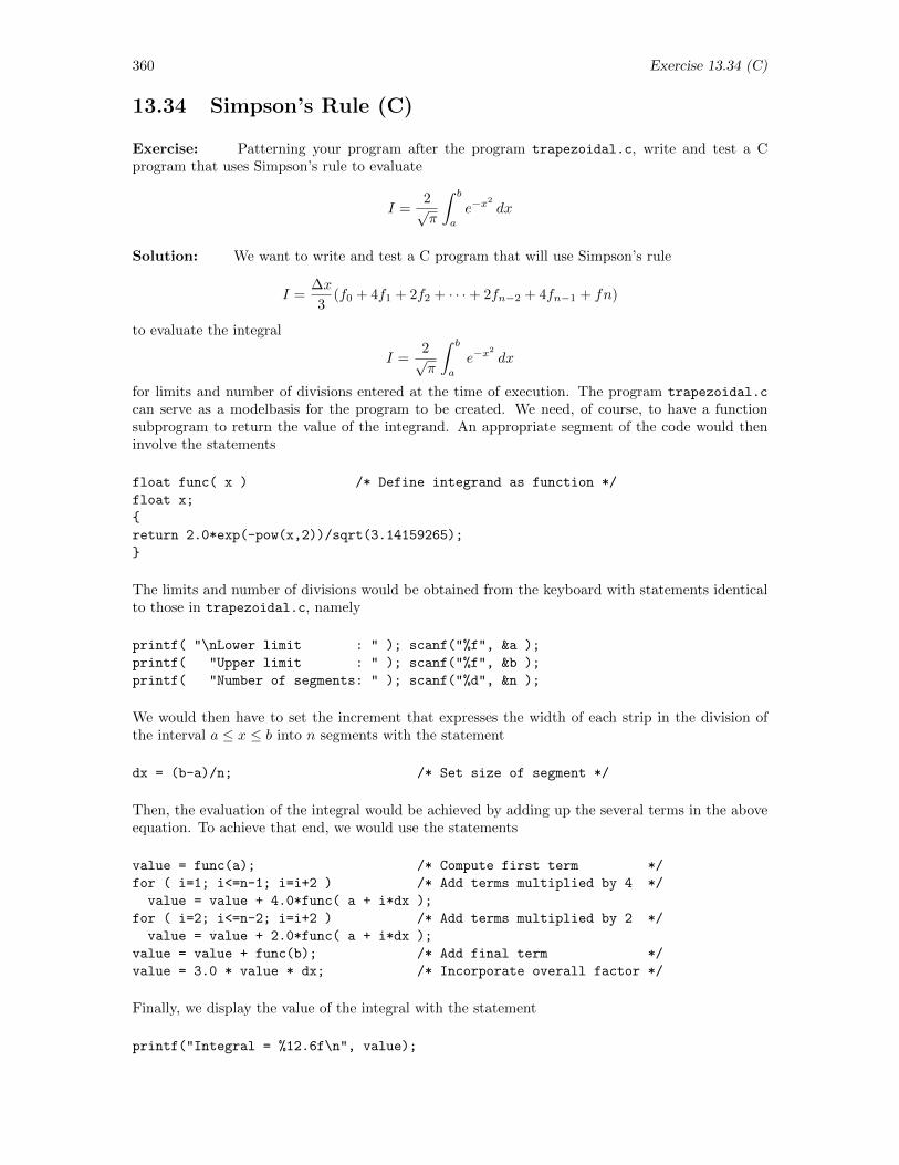
360 Exercise 13.34 (C)
13.34 Simpson’s Rule (C)
Exercise: Patterning your program after the program trapezoidal.c, write and test a Cprogram that uses Simpson’s rule to evaluate
I =2√π
∫ b
a
e−x2
dx
Solution: We want to write and test a C program that will use Simpson’s rule
I =∆x
3(f0 + 4f1 + 2f2 + · · ·+ 2fn−2 + 4fn−1 + fn)
to evaluate the integral
I =2√π
∫ b
a
e−x2
dx
for limits and number of divisions entered at the time of execution. The program trapezoidal.c
can serve as a modelbasis for the program to be created. We need, of course, to have a functionsubprogram to return the value of the integrand. An appropriate segment of the code would theninvolve the statements
float func( x ) /* Define integrand as function */
float x;
return 2.0*exp(-pow(x,2))/sqrt(3.14159265);
The limits and number of divisions would be obtained from the keyboard with statements identicalto those in trapezoidal.c, namely
printf( "\nLower limit : " ); scanf("%f", &a );
printf( "Upper limit : " ); scanf("%f", &b );
printf( "Number of segments: " ); scanf("%d", &n );
We would then have to set the increment that expresses the width of each strip in the division ofthe interval a ≤ x ≤ b into n segments with the statement
dx = (b-a)/n; /* Set size of segment */
Then, the evaluation of the integral would be achieved by adding up the several terms in the aboveequation. To achieve that end, we would use the statements
value = func(a); /* Compute first term */
for ( i=1; i<=n-1; i=i+2 ) /* Add terms multiplied by 4 */
value = value + 4.0*func( a + i*dx );
for ( i=2; i<=n-2; i=i+2 ) /* Add terms multiplied by 2 */
value = value + 2.0*func( a + i*dx );
value = value + func(b); /* Add final term */
value = 3.0 * value * dx; /* Incorporate overall factor */
Finally, we display the value of the integral with the statement
printf("Integral = %12.6f\n", value);
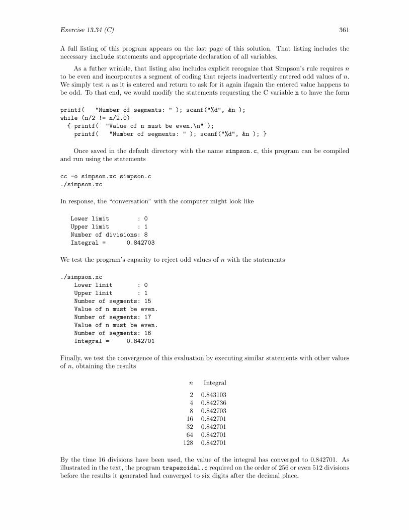
Exercise 13.34 (C) 361
A full listing of this program appears on the last page of this solution. That listing includes thenecessary include statements and appropriate declaration of all variables.
As a futher wrinkle, that listing also includes explicit recognize that Simpson’s rule requires nto be even and incorporates a segment of coding that rejects inadvertently entered odd values of n.We simply test n as it is entered and return to ask for it again ifagain the entered value happens tobe odd. To that end, we would modify the statements requesting the C variable n to have the form
printf( "Number of segments: " ); scanf("%d", &n );
while (n/2 != n/2.0)
printf( "Value of n must be even.\n" );
printf( "Number of segments: " ); scanf("%d", &n );
Once saved in the default directory with the name simpson.c, this program can be compiledand run using the statements
cc -o simpson.xc simpson.c
./simpson.xc
In response, the “conversation” with the computer might look like
Lower limit : 0
Upper limit : 1
Number of divisions: 8
Integral = 0.842703
We test the program’s capacity to reject odd values of n with the statements
./simpson.xc
Lower limit : 0
Upper limit : 1
Number of segments: 15
Value of n must be even.
Number of segments: 17
Value of n must be even.
Number of segments: 16
Integral = 0.842701
Finally, we test the convergence of this evaluation by executing similar statements with other valuesof n, obtaining the results
n Integral
2 0.8431034 0.8427368 0.842703
16 0.84270132 0.84270164 0.842701
128 0.842701
By the time 16 divisions have been used, the value of the integral has converged to 0.842701. Asillustrated in the text, the program trapezoidal.c required on the order of 256 or even 512 divisionsbefore the results it generated had converged to six digits after the decimal place.
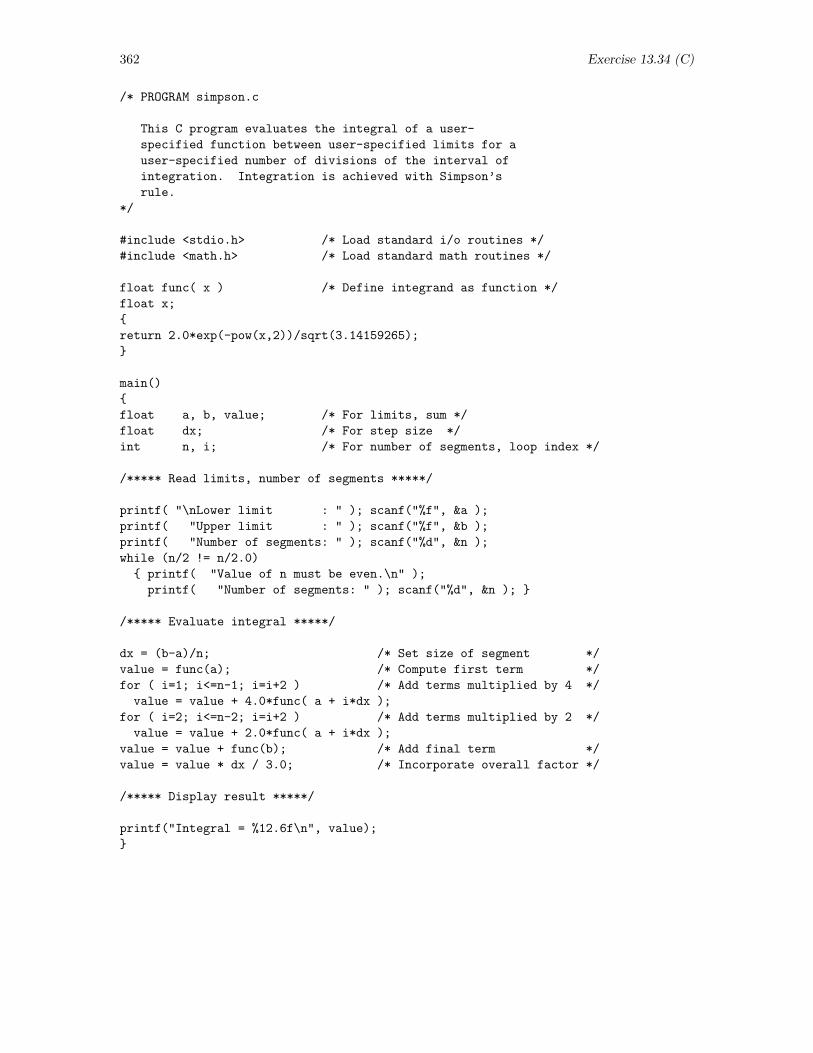
362 Exercise 13.34 (C)
/* PROGRAM simpson.c
This C program evaluates the integral of a user-
specified function between user-specified limits for a
user-specified number of divisions of the interval of
integration. Integration is achieved with Simpson’s
rule.
*/
#include <stdio.h> /* Load standard i/o routines */
#include <math.h> /* Load standard math routines */
float func( x ) /* Define integrand as function */
float x;
return 2.0*exp(-pow(x,2))/sqrt(3.14159265);
main()
float a, b, value; /* For limits, sum */
float dx; /* For step size */
int n, i; /* For number of segments, loop index */
/***** Read limits, number of segments *****/
printf( "\nLower limit : " ); scanf("%f", &a );
printf( "Upper limit : " ); scanf("%f", &b );
printf( "Number of segments: " ); scanf("%d", &n );
while (n/2 != n/2.0)
printf( "Value of n must be even.\n" );
printf( "Number of segments: " ); scanf("%d", &n );
/***** Evaluate integral *****/
dx = (b-a)/n; /* Set size of segment */
value = func(a); /* Compute first term */
for ( i=1; i<=n-1; i=i+2 ) /* Add terms multiplied by 4 */
value = value + 4.0*func( a + i*dx );
for ( i=2; i<=n-2; i=i+2 ) /* Add terms multiplied by 2 */
value = value + 2.0*func( a + i*dx );
value = value + func(b); /* Add final term */
value = value * dx / 3.0; /* Incorporate overall factor */
/***** Display result *****/
printf("Integral = %12.6f\n", value);
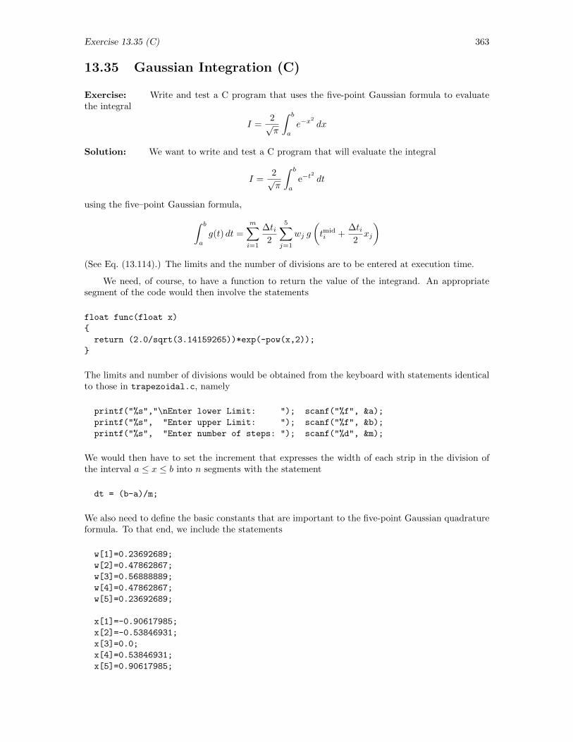
Exercise 13.35 (C) 363
13.35 Gaussian Integration (C)
Exercise: Write and test a C program that uses the five-point Gaussian formula to evaluatethe integral
I =2√π
∫ b
a
e−x2
dx
Solution: We want to write and test a C program that will evaluate the integral
I =2√π
∫ b
a
e−t2
dt
using the five–point Gaussian formula,∫ b
a
g(t) dt =
m∑i=1
∆ti2
5∑j=1
wj g
(tmidi +
∆ti2xj
)
(See Eq. (13.114).) The limits and the number of divisions are to be entered at execution time.
We need, of course, to have a function to return the value of the integrand. An appropriatesegment of the code would then involve the statements
float func(float x)
return (2.0/sqrt(3.14159265))*exp(-pow(x,2));
The limits and number of divisions would be obtained from the keyboard with statements identicalto those in trapezoidal.c, namely
printf("%s","\nEnter lower Limit: "); scanf("%f", &a);
printf("%s", "Enter upper Limit: "); scanf("%f", &b);
printf("%s", "Enter number of steps: "); scanf("%d", &m);
We would then have to set the increment that expresses the width of each strip in the division ofthe interval a ≤ x ≤ b into n segments with the statement
dt = (b-a)/m;
We also need to define the basic constants that are important to the five-point Gaussian quadratureformula. To that end, we include the statements
w[1]=0.23692689;
w[2]=0.47862867;
w[3]=0.56888889;
w[4]=0.47862867;
w[5]=0.23692689;
x[1]=-0.90617985;
x[2]=-0.53846931;
x[3]=0.0;
x[4]=0.53846931;
x[5]=0.90617985;
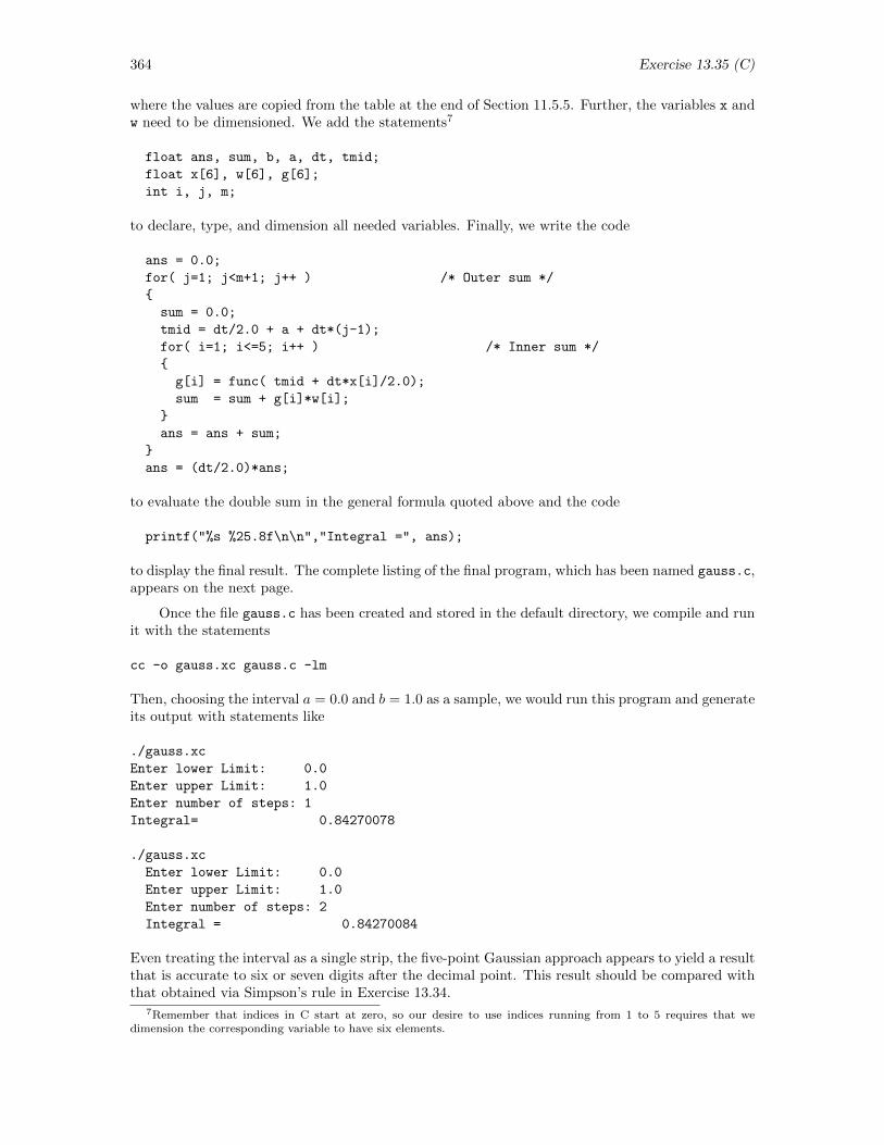
364 Exercise 13.35 (C)
where the values are copied from the table at the end of Section 11.5.5. Further, the variables x andw need to be dimensioned. We add the statements7
float ans, sum, b, a, dt, tmid;
float x[6], w[6], g[6];
int i, j, m;
to declare, type, and dimension all needed variables. Finally, we write the code
ans = 0.0;
for( j=1; j<m+1; j++ ) /* Outer sum */
sum = 0.0;
tmid = dt/2.0 + a + dt*(j-1);
for( i=1; i<=5; i++ ) /* Inner sum */
g[i] = func( tmid + dt*x[i]/2.0);
sum = sum + g[i]*w[i];
ans = ans + sum;
ans = (dt/2.0)*ans;
to evaluate the double sum in the general formula quoted above and the code
printf("%s %25.8f\n\n","Integral =", ans);
to display the final result. The complete listing of the final program, which has been named gauss.c,appears on the next page.
Once the file gauss.c has been created and stored in the default directory, we compile and runit with the statements
cc -o gauss.xc gauss.c -lm
Then, choosing the interval a = 0.0 and b = 1.0 as a sample, we would run this program and generateits output with statements like
./gauss.xc
Enter lower Limit: 0.0
Enter upper Limit: 1.0
Enter number of steps: 1
Integral= 0.84270078
./gauss.xc
Enter lower Limit: 0.0
Enter upper Limit: 1.0
Enter number of steps: 2
Integral = 0.84270084
Even treating the interval as a single strip, the five-point Gaussian approach appears to yield a resultthat is accurate to six or seven digits after the decimal point. This result should be compared withthat obtained via Simpson’s rule in Exercise 13.34.
7Remember that indices in C start at zero, so our desire to use indices running from 1 to 5 requires that wedimension the corresponding variable to have six elements.
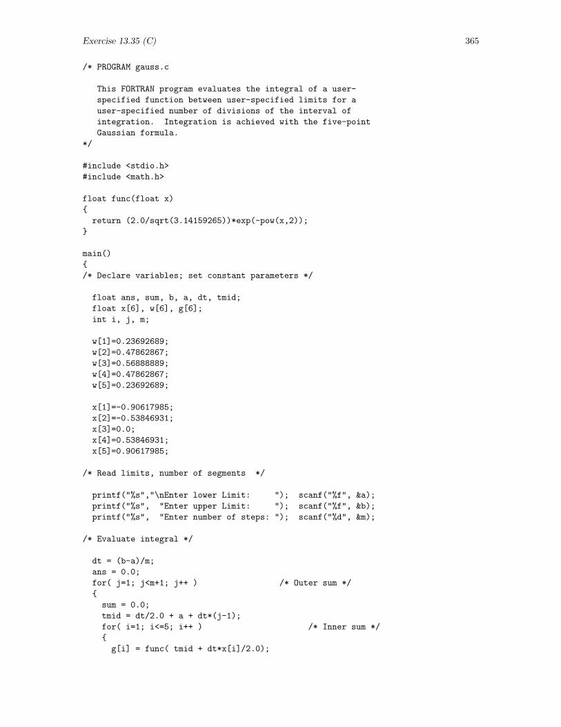
Exercise 13.35 (C) 365
/* PROGRAM gauss.c
This FORTRAN program evaluates the integral of a user-
specified function between user-specified limits for a
user-specified number of divisions of the interval of
integration. Integration is achieved with the five-point
Gaussian formula.
*/
#include <stdio.h>
#include <math.h>
float func(float x)
return (2.0/sqrt(3.14159265))*exp(-pow(x,2));
main()
/* Declare variables; set constant parameters */
float ans, sum, b, a, dt, tmid;
float x[6], w[6], g[6];
int i, j, m;
w[1]=0.23692689;
w[2]=0.47862867;
w[3]=0.56888889;
w[4]=0.47862867;
w[5]=0.23692689;
x[1]=-0.90617985;
x[2]=-0.53846931;
x[3]=0.0;
x[4]=0.53846931;
x[5]=0.90617985;
/* Read limits, number of segments */
printf("%s","\nEnter lower Limit: "); scanf("%f", &a);
printf("%s", "Enter upper Limit: "); scanf("%f", &b);
printf("%s", "Enter number of steps: "); scanf("%d", &m);
/* Evaluate integral */
dt = (b-a)/m;
ans = 0.0;
for( j=1; j<m+1; j++ ) /* Outer sum */
sum = 0.0;
tmid = dt/2.0 + a + dt*(j-1);
for( i=1; i<=5; i++ ) /* Inner sum */
g[i] = func( tmid + dt*x[i]/2.0);

366 Exercise 13.35 (C)
sum = sum + g[i]*w[i];
ans = ans + sum;
ans = (dt/2.0)*ans;
/* Display result */
printf("%s %25.8f\n\n","Integral =", ans);
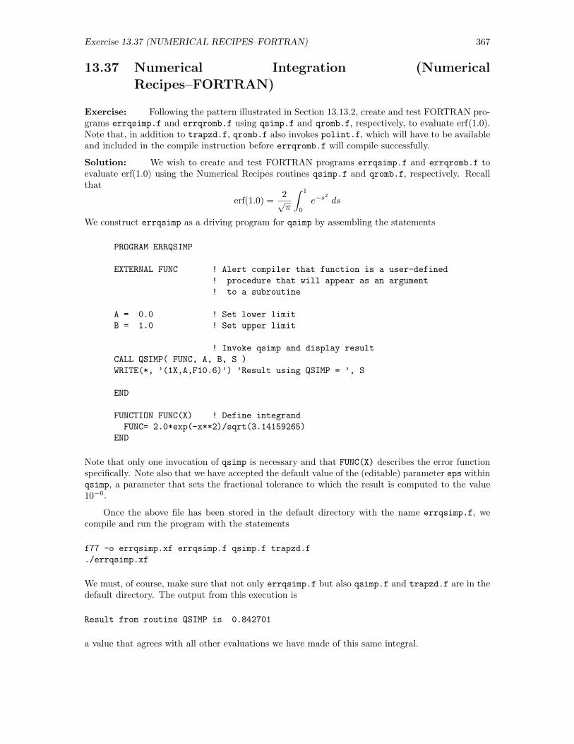
Exercise 13.37 (NUMERICAL RECIPES–FORTRAN) 367
13.37 Numerical Integration (NumericalRecipes–FORTRAN)
Exercise: Following the pattern illustrated in Section 13.13.2, create and test FORTRAN pro-grams errqsimp.f and errqromb.f using qsimp.f and qromb.f, respectively, to evaluate erf(1.0).Note that, in addition to trapzd.f, qromb.f also invokes polint.f, which will have to be availableand included in the compile instruction before errqromb.f will compile successfully.
Solution: We wish to create and test FORTRAN programs errqsimp.f and errqromb.f toevaluate erf(1.0) using the Numerical Recipes routines qsimp.f and qromb.f, respectively. Recallthat
erf(1.0) =2√π
∫ 1
0
e−s2
ds
We construct errqsimp as a driving program for qsimp by assembling the statements
PROGRAM ERRQSIMP
EXTERNAL FUNC ! Alert compiler that function is a user-defined
! procedure that will appear as an argument
! to a subroutine
A = 0.0 ! Set lower limit
B = 1.0 ! Set upper limit
! Invoke qsimp and display result
CALL QSIMP( FUNC, A, B, S )
WRITE(*, ’(1X,A,F10.6)’) ’Result using QSIMP = ’, S
END
FUNCTION FUNC(X) ! Define integrand
FUNC= 2.0*exp(-x**2)/sqrt(3.14159265)
END
Note that only one invocation of qsimp is necessary and that FUNC(X) describes the error functionspecifically. Note also that we have accepted the default value of the (editable) parameter eps withinqsimp, a parameter that sets the fractional tolerance to which the result is computed to the value10−6.
Once the above file has been stored in the default directory with the name errqsimp.f, wecompile and run the program with the statements
f77 -o errqsimp.xf errqsimp.f qsimp.f trapzd.f
./errqsimp.xf
We must, of course, make sure that not only errqsimp.f but also qsimp.f and trapzd.f are in thedefault directory. The output from this execution is
Result from routine QSIMP is 0.842701
a value that agrees with all other evaluations we have made of this same integral.
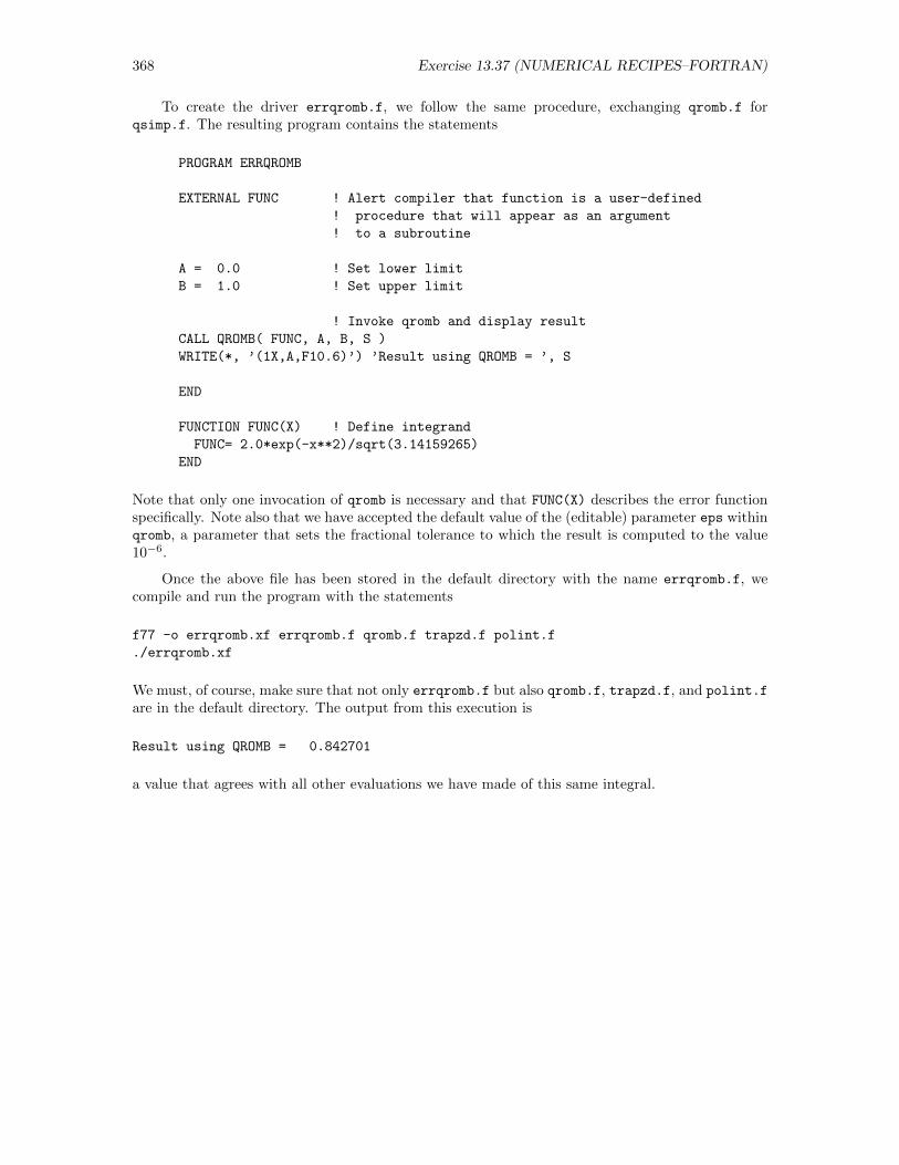
368 Exercise 13.37 (NUMERICAL RECIPES–FORTRAN)
To create the driver errqromb.f, we follow the same procedure, exchanging qromb.f forqsimp.f. The resulting program contains the statements
PROGRAM ERRQROMB
EXTERNAL FUNC ! Alert compiler that function is a user-defined
! procedure that will appear as an argument
! to a subroutine
A = 0.0 ! Set lower limit
B = 1.0 ! Set upper limit
! Invoke qromb and display result
CALL QROMB( FUNC, A, B, S )
WRITE(*, ’(1X,A,F10.6)’) ’Result using QROMB = ’, S
END
FUNCTION FUNC(X) ! Define integrand
FUNC= 2.0*exp(-x**2)/sqrt(3.14159265)
END
Note that only one invocation of qromb is necessary and that FUNC(X) describes the error functionspecifically. Note also that we have accepted the default value of the (editable) parameter eps withinqromb, a parameter that sets the fractional tolerance to which the result is computed to the value10−6.
Once the above file has been stored in the default directory with the name errqromb.f, wecompile and run the program with the statements
f77 -o errqromb.xf errqromb.f qromb.f trapzd.f polint.f
./errqromb.xf
We must, of course, make sure that not only errqromb.f but also qromb.f, trapzd.f, and polint.f
are in the default directory. The output from this execution is
Result using QROMB = 0.842701
a value that agrees with all other evaluations we have made of this same integral.
Exercise 13.40 (NUMERICAL RECIPES–FORTRAN) 369
13.40 Maxwell-Boltzmann Distribution (NumericalRecipes–FORTRAN)
Exercise: Use trapzd.f, qtrap.f, qsimp.f, and qromb.f in a succession of programs toevaluate the quantity
f(v) =
∫ v
0
v′2 e−v′2/2 dv
(a) for v = 1.0 and (b) as a function of v over the range 0.0 ≤ v ≤ 3.0. Cast your response topart (b) so that it writes the values of v and f(v) into a (text) file that could then be importedinto another program for graphical display. Statements for opening, writing to, and closing a file inFORTRAN are introduced in the chapter of CPSUP titled “Introduction to Programming”.
Solution: To evaluate the quantity
f(v) =
∫ v
0
v′2 e−v′2/2 dv
a) for v = 1.0, we modify the driving program errtrapzd.f mentioned earlier in the chapter so thatthe function reads
FUNCTION FUNC(X) ! Define integrand
FUNC=X**2*EXP(-X**2/2.0)
END
Then we can compile, link and run ertrapzd.xf (since all the other subroutines are presumablystill in the default directory from the exercises in the chapter) with the statements
f77 -o errtrapzd.xf errtrapzd.f trapzd.f
./errtrapzd.xf
n No Divs Approx. Integral
1 1 0.303265
2 2 0.261945
3 4 0.252266
4 8 0.249884
5 16 0.249291
6 32 0.249143
7 64 0.249106
8 128 0.249097
9 256 0.249095
10 512 0.249094
11 1024 0.249094
12 2048 0.249094
13 4096 0.249094
14 8192 0.249094
and we can conclude that the value of the integral is 0.249094 (to six digits).
We modify the functions in errqtrap.f, errqsimp.f and errqromb.f in the same way, thencompile, link and run them with the statements
f77 -o errqtrap.xf errqtrap.f trapzd.f qtrap.f
./errqtrap.xf
Result using QTRAP = 0.249094
370 Exercise 13.40 (NUMERICAL RECIPES–FORTRAN)
f77 -o errqsimp.xf errqsimp.f trapzd.f qsimp.f
./errqsimp.xf
Result using QSIMP = 0.249094
f77 -o errqromb.xf errqromb.f trapzd.f qromb.f polint.f
./errqromb.xf
Result using QROMB = 0.249094
Happily, the results all agree with each other.
b) To evaluate the quantity as a function of v over the range 0.0 ≤ v ≤ 3.0, we modify the programerrtrapzd.f to become this:
PROGRAM ERRTRAPZD
EXTERNAL FUNC ! Alert compiler that FUNC is a user-defined
! procedure that will appear as an argument
! to a subroutine
NUMIT = 14 ! Set number of iterations
A = 0.0 ! Set lower limit
! Open file to put data in
OPEN( UNIT = 1, FILE = ’errtrapzd_f.dat’, STATUS=’NEW’)
DO J = 0, 1000 ! Loop to evaluate over a range of upper
B = J*0.003 ! limits from 0 to 3 with 1000 steps
DO I = 1,NUMIT
! Invoke TRAPZD
CALL TRAPZD( FUNC, A, B, S, I )
ENDDO
! Write the results to file
WRITE(1, ’(F20.6,F20.6)’) B, S
ENDDO
CLOSE( UNIT = 1 ) ! Close the file
END
FUNCTION FUNC(X) ! Define integrand
FUNC= X**2*EXP(-X**2/2.0)
END
We then compile, link and run this program with the statements
f77 -o errtrapzd.xf errtrapzd.f trapzd.f
./errtrapzd.xf
Next, we modify the program errqtrap.f in the same way to become
PROGRAM ERRQTRAP
EXTERNAL FUNC ! Alert compiler that FUNC is a user-defined
! procedure that will appear as an argument
! to a subroutine
A = 0.0 ! Set lower limit
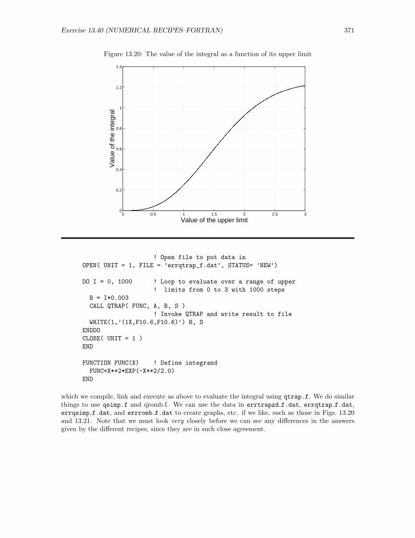
Exercise 13.40 (NUMERICAL RECIPES–FORTRAN) 371
Figure 13.20: The value of the integral as a function of its upper limit
0 0.5 1 1.5 2 2.5 30
0.2
0.4
0.6
0.8
1
1.2
1.4
Value of the upper limit
Val
ue o
f the
inte
gral
! Open file to put data in
OPEN( UNIT = 1, FILE = ’errqtrap_f.dat’, STATUS= ’NEW’)
DO I = 0, 1000 ! Loop to evaluate over a range of upper
! limits from 0 to 3 with 1000 steps
B = I*0.003
CALL QTRAP( FUNC, A, B, S )
! Invoke QTRAP and write result to file
WRITE(1,’(1X,F10.6,F10.6)’) B, S
ENDDO
CLOSE( UNIT = 1 )
END
FUNCTION FUNC(X) ! Define integrand
FUNC=X**2*EXP(-X**2/2.0)
END
which we compile, link and execute as above to evaluate the integral using qtrap.f. We do similarthings to use qsimp.f and qromb.f. We can use the data in errtrapzd f.dat, errqtrap f.dat,errqsimp f.dat, and errromb f.dat to create graphs, etc. if we like, such as those in Figs. 13.20and 13.21. Note that we must look very closely before we can see any differences in the answersgiven by the different recipes, since they are in such close agreement.
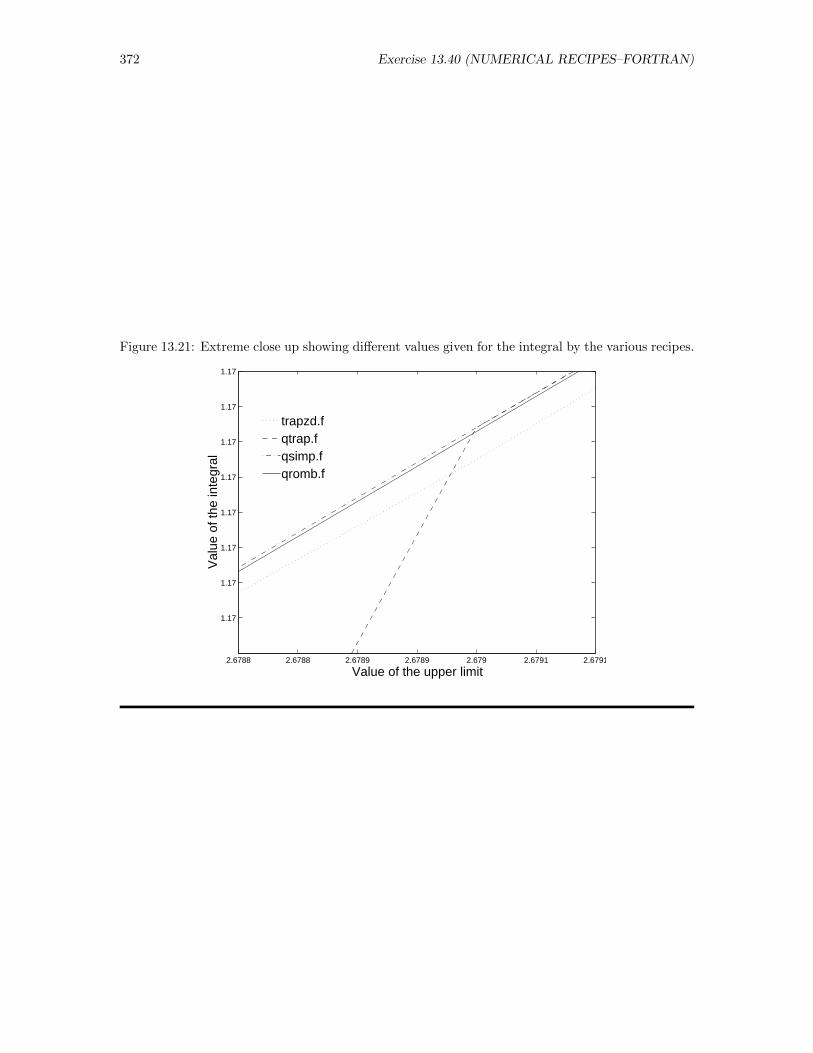
372 Exercise 13.40 (NUMERICAL RECIPES–FORTRAN)
Figure 13.21: Extreme close up showing different values given for the integral by the various recipes.
2.6788 2.6788 2.6789 2.6789 2.679 2.6791 2.6791
1.17
1.17
1.17
1.17
1.17
1.17
1.17
1.17
Value of the upper limit
Val
ue o
f the
inte
gral
qromb.fqsimp.fqtrap.ftrapzd.f
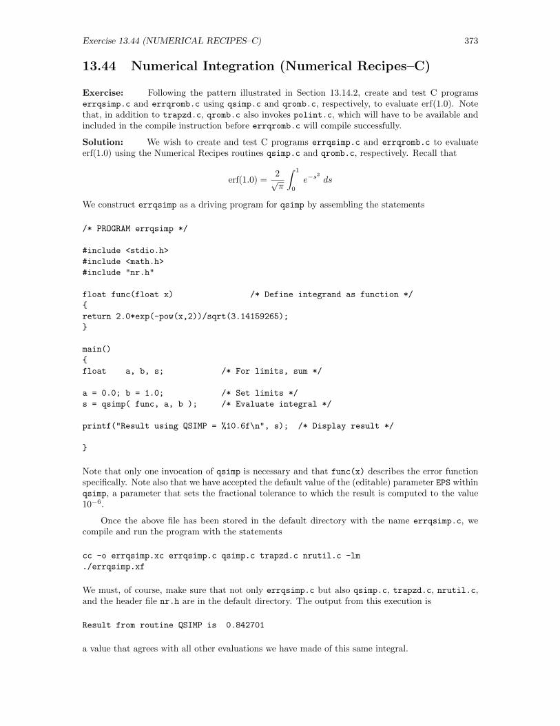
Exercise 13.44 (NUMERICAL RECIPES–C) 373
13.44 Numerical Integration (Numerical Recipes–C)
Exercise: Following the pattern illustrated in Section 13.14.2, create and test C programserrqsimp.c and errqromb.c using qsimp.c and qromb.c, respectively, to evaluate erf(1.0). Notethat, in addition to trapzd.c, qromb.c also invokes polint.c, which will have to be available andincluded in the compile instruction before errqromb.c will compile successfully.
Solution: We wish to create and test C programs errqsimp.c and errqromb.c to evaluateerf(1.0) using the Numerical Recipes routines qsimp.c and qromb.c, respectively. Recall that
erf(1.0) =2√π
∫ 1
0
e−s2
ds
We construct errqsimp as a driving program for qsimp by assembling the statements
/* PROGRAM errqsimp */
#include <stdio.h>
#include <math.h>
#include "nr.h"
float func(float x) /* Define integrand as function */
return 2.0*exp(-pow(x,2))/sqrt(3.14159265);
main()
float a, b, s; /* For limits, sum */
a = 0.0; b = 1.0; /* Set limits */
s = qsimp( func, a, b ); /* Evaluate integral */
printf("Result using QSIMP = %10.6f\n", s); /* Display result */
Note that only one invocation of qsimp is necessary and that func(x) describes the error functionspecifically. Note also that we have accepted the default value of the (editable) parameter EPS withinqsimp, a parameter that sets the fractional tolerance to which the result is computed to the value10−6.
Once the above file has been stored in the default directory with the name errqsimp.c, wecompile and run the program with the statements
cc -o errqsimp.xc errqsimp.c qsimp.c trapzd.c nrutil.c -lm
./errqsimp.xf
We must, of course, make sure that not only errqsimp.c but also qsimp.c, trapzd.c, nrutil.c,and the header file nr.h are in the default directory. The output from this execution is
Result from routine QSIMP is 0.842701
a value that agrees with all other evaluations we have made of this same integral.
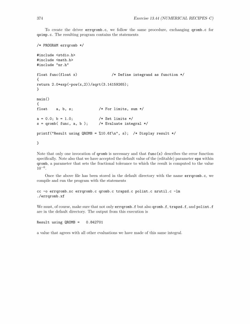
374 Exercise 13.44 (NUMERICAL RECIPES–C)
To create the driver errqromb.c, we follow the same procedure, exchanging qromb.c forqsimp.c. The resulting program contains the statements
/* PROGRAM errqromb */
#include <stdio.h>
#include <math.h>
#include "nr.h"
float func(float x) /* Define integrand as function */
return 2.0*exp(-pow(x,2))/sqrt(3.14159265);
main()
float a, b, s; /* For limits, sum */
a = 0.0; b = 1.0; /* Set limits */
s = qromb( func, a, b ); /* Evaluate integral */
printf("Result using QROMB = %10.6f\n", s); /* Display result */
Note that only one invocation of qromb is necessary and that func(x) describes the error functionspecifically. Note also that we have accepted the default value of the (editable) parameter eps withinqromb, a parameter that sets the fractional tolerance to which the result is computed to the value10−6.
Once the above file has been stored in the default directory with the name errqromb.c, wecompile and run the program with the statements
cc -o errqromb.xc errqromb.c qromb.c trapzd.c polint.c nrutil.c -lm
./errqromb.xf
We must, of course, make sure that not only errqromb.f but also qromb.f, trapzd.f, and polint.f
are in the default directory. The output from this execution is
Result using QROMB = 0.842701
a value that agrees with all other evaluations we have made of this same integral.
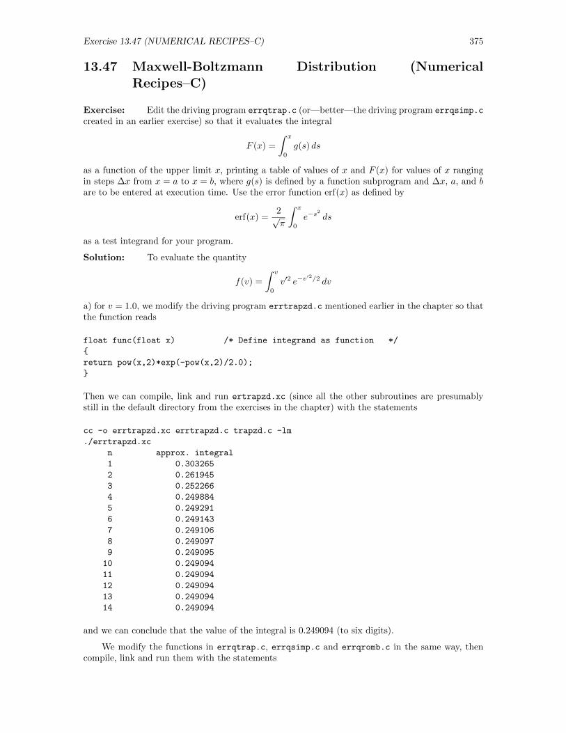
Exercise 13.47 (NUMERICAL RECIPES–C) 375
13.47 Maxwell-Boltzmann Distribution (NumericalRecipes–C)
Exercise: Edit the driving program errqtrap.c (or—better—the driving program errqsimp.c
created in an earlier exercise) so that it evaluates the integral
F (x) =
∫ x
0
g(s) ds
as a function of the upper limit x, printing a table of values of x and F (x) for values of x rangingin steps ∆x from x = a to x = b, where g(s) is defined by a function subprogram and ∆x, a, and bare to be entered at execution time. Use the error function erf(x) as defined by
erf(x) =2√π
∫ x
0
e−s2
ds
as a test integrand for your program.
Solution: To evaluate the quantity
f(v) =
∫ v
0
v′2 e−v′2/2 dv
a) for v = 1.0, we modify the driving program errtrapzd.c mentioned earlier in the chapter so thatthe function reads
float func(float x) /* Define integrand as function */
return pow(x,2)*exp(-pow(x,2)/2.0);
Then we can compile, link and run ertrapzd.xc (since all the other subroutines are presumablystill in the default directory from the exercises in the chapter) with the statements
cc -o errtrapzd.xc errtrapzd.c trapzd.c -lm
./errtrapzd.xc
n approx. integral
1 0.303265
2 0.261945
3 0.252266
4 0.249884
5 0.249291
6 0.249143
7 0.249106
8 0.249097
9 0.249095
10 0.249094
11 0.249094
12 0.249094
13 0.249094
14 0.249094
and we can conclude that the value of the integral is 0.249094 (to six digits).
We modify the functions in errqtrap.c, errqsimp.c and errqromb.c in the same way, thencompile, link and run them with the statements
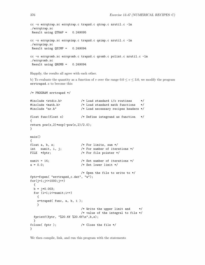
376 Exercise 13.47 (NUMERICAL RECIPES–C)
cc -o errqtrap.xc errqtrap.c trapzd.c qtrap.c nrutil.c -lm
./errqtrap.xc
Result using QTRAP = 0.249095
cc -o errqsimp.xc errqsimp.c trapzd.c qsimp.c nrutil.c -lm
./errqsimp.xc
Result using QSIMP = 0.249094
cc -o errqromb.xc errqromb.c trapzd.c qromb.c polint.c nrutil.c -lm
./errqromb.xc
Result using QROMB = 0.249094
Happily, the results all agree with each other.
b) To evaluate the quantity as a function of v over the range 0.0 ≤ v ≤ 3.0, we modify the programerrtrapzd.c to become this:
/* PROGRAM errtrapzd */
#include <stdio.h> /* Load standard i/o routines */
#include <math.h> /* Load standard math functions */
#include "nr.h" /* Load necessary recipes headers */
float func(float x) /* Define integrand as function */
return pow(x,2)*exp(-pow(x,2)/2.0);
main()
float a, b, s; /* For limits, sum */
int numit, i, j; /* For number of iterations */
FILE *fptr; /* For file pointer */
numit = 14; /* Set number of iterations */
a = 0.0; /* Set lower limit */
/* Open the file to write to */
fptr=fopen( "errtrapzd_c.dat", "w");
for(j=1;j<=1000;j++)
b = j*0.003;
for (i=1;i<=numit;i++)
s=trapzd( func, a, b, i );
/* Write the upper limit and */
/* value of the integral to file */
fprintf(fptr, "%20.6f %20.6f\n",b,s);
fclose( fptr ); /* Close the file */
We then compile, link, and run this program with the statements
Exercise 13.47 (NUMERICAL RECIPES–C) 377
cc -o errtrapzd.xc errtrapzd.c trapzd.c -lm
./errtrapzd.xc
Next, we modify the program errqtrap.c in the same way to become
/* PROGRAM errqtrap */
#include <stdio.h> /* Load standard i/o routines */
#include <math.h> /* Load standard math routines */
#include "nr.h" /* Load necessary recipes headers */
float func(float x) /* Define integrand as function */
return pow(x,2)*exp(-pow(x,2)/2.0);
main()
float a, b, s; /* For limits, sum */
int i; /* For iterations */
FILE *fptr; /* For file pointer */
a = 0.0; /* Set lower limit */
/* Open the file to write to */
fptr=fopen( "errqtrap_c.dat", "w");
for(i=1;i<=1000;i++)
b = i*0.003;
s = qtrap( func, a, b ); /* Evaluate integral */
/* Write the upper limit and */
/* value of the integral to file */
fprintf(fptr, "%20.6f %20.6f\n",b,s);
fclose( fptr ); /* Close the file */
which we compile, link and execute as above to evaluate the integral using qtrap.c. We do similarthings to use qsimp.c and qromb.c. We can use the data in errtrapzd c.dat, errqtrap c.dat,errqsimp c.dat, and errromb c.dat to create graphs, etc. if we like, such as those in Figs. 13.22and 13.23. Note, in Fig. 13.23, that we must look very closely before we can see any differences inthe answers given by the various recipes, since they are in such close agreement.
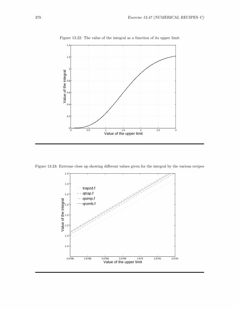
378 Exercise 13.47 (NUMERICAL RECIPES–C)
Figure 13.22: The value of the integral as a function of its upper limit
0 0.5 1 1.5 2 2.5 30
0.2
0.4
0.6
0.8
1
1.2
1.4
Value of the upper limit
Val
ue o
f the
inte
gral
Figure 13.23: Extreme close up showing different values given for the integral by the various recipes
2.6788 2.6788 2.6789 2.6789 2.679 2.6791 2.6791
1.17
1.17
1.17
1.17
1.17
1.17
1.17
1.17
Value of the upper limit
Val
ue o
f the
inte
gral
qromb.fqsimp.fqtrap.ftrapzd.f
Chapter 14
Finding Roots
14.3 Finding Extrema a Cubic Polynomial (Mathematica)
Exercise: Find the points at which the function f(x) = ax3 + bx2 + cx+ d has (local) extremaand find a criterion involving the coefficients (or some of them) that will assure that the functionhas three real roots. Assume that a, b, c, and d are real.
Solution: We seek the extreme points of f(x) = ax3 + bx2 + cx + d. We enter this equationinto Mathematica with the statement
In[1]:= eq = a*x^3 + b*x^2 + c*x + d;
Then we find the roots of the first derivative with the statements
In[2]:= deq = D[ eq, x ];
In[3]:= soln = Solve[ deq == 0, x ];
In[4]:= soln1 = soln[[1]][[1]]
Out[4]= x→ −b−√b2 − 3ac
3a
In[5]:= soln2 = soln[[2]][[1]]
Out[5]= x→ −b+√b2 − 3ac
3a
These are the values of x at which the polynomial eq has a (local) maximum or a (local) minimum.The values of eq at these points are given by
In[6]:= ext1 = Simplify[ eq /. soln1 ]
Out[6]=2b3 − 9abc+ 2b2
√b2 − 3ac− 6ac
√b2 − 3ac+ 27a2d
27a2
In[7]:= ext2 = Simplify[ eq /. soln2 ]
Out[7]=2b3 − 9abc− 2b2
√b2 − 3ac+ 6ac
√b2 − 3ac+ 27a2d
27a2
We know that if all three roots of eq are real, then the two extreme points must also be real.This means that the quantity under the square root, b2 − 3ca, in both solutions must be positive.We also know that if all three roots are real, then the product of the two extreme points ought to be
379
380 Exercise 14.3 (Mathematica)
negative, i.e., the value of eq at the maximun extreme point and its value at the minimum extremepoint must have opposite signs. To see what restrictions this additional criterion puts on a, b, c andd, we begin by evaluating the critical product with the statements
In[8]:= prod = Simplify[ ext1 * ext2 ]
Out[8]=−b2c2 + 4b3d− 18abcd+ a
(4c3 + 27ad2
)27a2
Since both 27 and a2 are positive, we can multiply this result by 27a2 without affecting its sign.Thus, we must require that the quantity given by
In[9]:= Expand[ 27*a^2*prod ]
Out[9]= −b2c2 + 4ac3 + 4b3d− 18abcd+ 27a2d2
be less than zero. In summary, we conclude that
• If b2 − 3ca < 0, the cubic polynomial has only one real root.
• If b2 − 3ca > 0, the cubic polynomial may have three real roots, but only if, in addition
−b2c2 + 4ac3 − 6abcd+ 27a2d2 < 0
Exercise 14.4 (Mathematica) 381
14.4 Roots of Quadratic Equation (Mathematica)
Exercise: In some quantum calculations, the need to solve the equation x(x+ 1) = l(l+ 1) forx arises. Find those roots, noting particularly that, since the equation is quadratic, there are tworoots. The obvious root x = l is not the only one.
Solution: We wish to find the roots to the equation x(x + 1) = l(l + 1) or, equivalently, tosolve x(x + 1) − l(l + 1) = 0 for x. To do this symbolically in Mathematica is a straight forwardcalculation. We simply define the expression and request its roots with the statements
In[1]:= eq = x*(x + 1) - l*(l + 1);
In[2]:= soln = Solve[eq == 0, x]
Out[2]=
x→ −1− l,x→ l
We see that there are two roots, which we expect for a quadratic equation. To verify these solutions,we substitute them into the original equation using the statements
In[3]:= eq /. x -> soln[[2, 1, 2]]
Out[3]= 0
In[4]:= eq /. x -> soln[[1, 1, 2]]
Out[4]= −(−1− l)l − l(1 + l)
In[5]:= Simplify[%]
Out[5]= 0
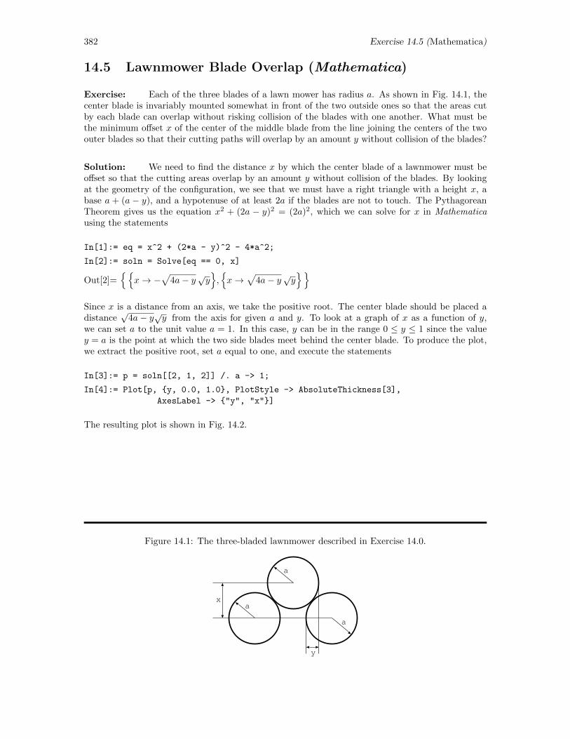
382 Exercise 14.5 (Mathematica)
14.5 Lawnmower Blade Overlap (Mathematica)
Exercise: Each of the three blades of a lawn mower has radius a. As shown in Fig. 14.1, thecenter blade is invariably mounted somewhat in front of the two outside ones so that the areas cutby each blade can overlap without risking collision of the blades with one another. What must bethe minimum offset x of the center of the middle blade from the line joining the centers of the twoouter blades so that their cutting paths will overlap by an amount y without collision of the blades?
Solution: We need to find the distance x by which the center blade of a lawnmower must beoffset so that the cutting areas overlap by an amount y without collision of the blades. By lookingat the geometry of the configuration, we see that we must have a right triangle with a height x, abase a + (a − y), and a hypotenuse of at least 2a if the blades are not to touch. The PythagoreanTheorem gives us the equation x2 + (2a − y)2 = (2a)2, which we can solve for x in Mathematicausing the statements
In[1]:= eq = x^2 + (2*a - y)^2 - 4*a^2;
In[2]:= soln = Solve[eq == 0, x]
Out[2]=
x→ −√
4a− y√y,x→
√4a− y√y
Since x is a distance from an axis, we take the positive root. The center blade should be placed adistance
√4a− y√y from the axis for given a and y. To look at a graph of x as a function of y,
we can set a to the unit value a = 1. In this case, y can be in the range 0 ≤ y ≤ 1 since the valuey = a is the point at which the two side blades meet behind the center blade. To produce the plot,we extract the positive root, set a equal to one, and execute the statements
In[3]:= p = soln[[2, 1, 2]] /. a -> 1;
In[4]:= Plot[p, y, 0.0, 1.0, PlotStyle -> AbsoluteThickness[3],
AxesLabel -> "y", "x"]
The resulting plot is shown in Fig. 14.2.
Figure 14.1: The three-bladed lawnmower described in Exercise 14.0.
a
a
a
x
y
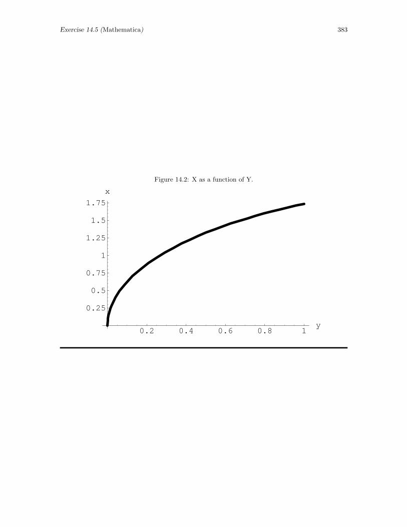
Exercise 14.5 (Mathematica) 383
Figure 14.2: X as a function of Y.
0.2 0.4 0.6 0.8 1y
0.25
0.5
0.75
1
1.25
1.5
1.75
x
384 Exercise 14.8 (Mathematica)
14.8 Three Coupled Oscillators (Mathematica)
Exercise: Find the natural frequencies for the three modes of oscillation characterizing thesystem that results when the system shown in Fig. ?? is extended to contain three objects coupledin a line. Take the four springs all to have the same spring constant but allow for the possibilitythat the middle object may have a mass m′ different from the mass m of the two outside objects. Inparticular, measure frequencies in units of
√k/m and seek a graph showing the frequency of each
of the modes as a function of β = m′/m. Hint : To help you get started and to facilitate focusing onthe solution of the ODEs rather than on deriving them, note that, for three masses, the equationsof motion will be
md2x1
dt2= −kx1 + k(x2 − x1)
m′d2x2
dt2= −k(x2 − x1) + k(x3 − x2)
md2x3
dt2= −k(x3 − x2)− kx3
Solution: Given the equations
md2x1
dt2= −kx1 + k(x2 − x1); m′
d2x2
dt2= −k(x2 − x1) + k(x3 − x2); m
d2x3
dt2= −k(x3 − x2)− kx3
for the motion of three objects connected by four springs, the substitutions ω0 =√k/m, β = m′/m,
and t = ω0t causes the equations to become
d2x1
dt2= −2x1 + x2; β
d2x1
dt2= x1 − 2x2 + x3;
d2x3
dt2= x2 − 2x3
We enter these into Mathematica using the statements
In[1]:= equ1 = x1’’[t] == -2*x1[t] + x2[t];
In[2]:= equ2 = \[Beta]*x2’’[t] == x1[t] - 2*x2[t] + x3[t];
In[3]:= equ3 = x3’’[t] == x2[t] - 2*x3[t];
We then assume solutions of the form x1 = x10 cosωt et al., and substitute these into the equationsto find the natural frequencies. To insure non-trivial solutions, we must require the determinantof the coefficient matrix to be zero. To extract that determinant and find its roots, we invoke thestatements
In[4]:= x1[t_] := x10*Cos[\[Omega]*t]
In[5]:= x2[t_] := x20*Cos[\[Omega]*t]
In[6]:= x3[t_] := x30*Cos[\[Omega]*t]
In[7]:= eq1 = Simplify[equ1]
Out[7]= (x20 + x10(−2 + ω2)) Cos [tω] == 0
In[8]:= eq2 = Simplify[equ2]
Out[8]= (x10 + x30 + x20(−2 + βω2)) Cos [tω] == 0
In[9]:= eq3 = Simplify[equ3]
Out[9]= (x20 + x30(−2 + ω2)) Cos [tω] == 0
In[10]:= eqn1 = eq1[[1]]/Cos[\[Omega]*t] == 0
Out[10]= x20 + x10(−2 + ω2) == 0
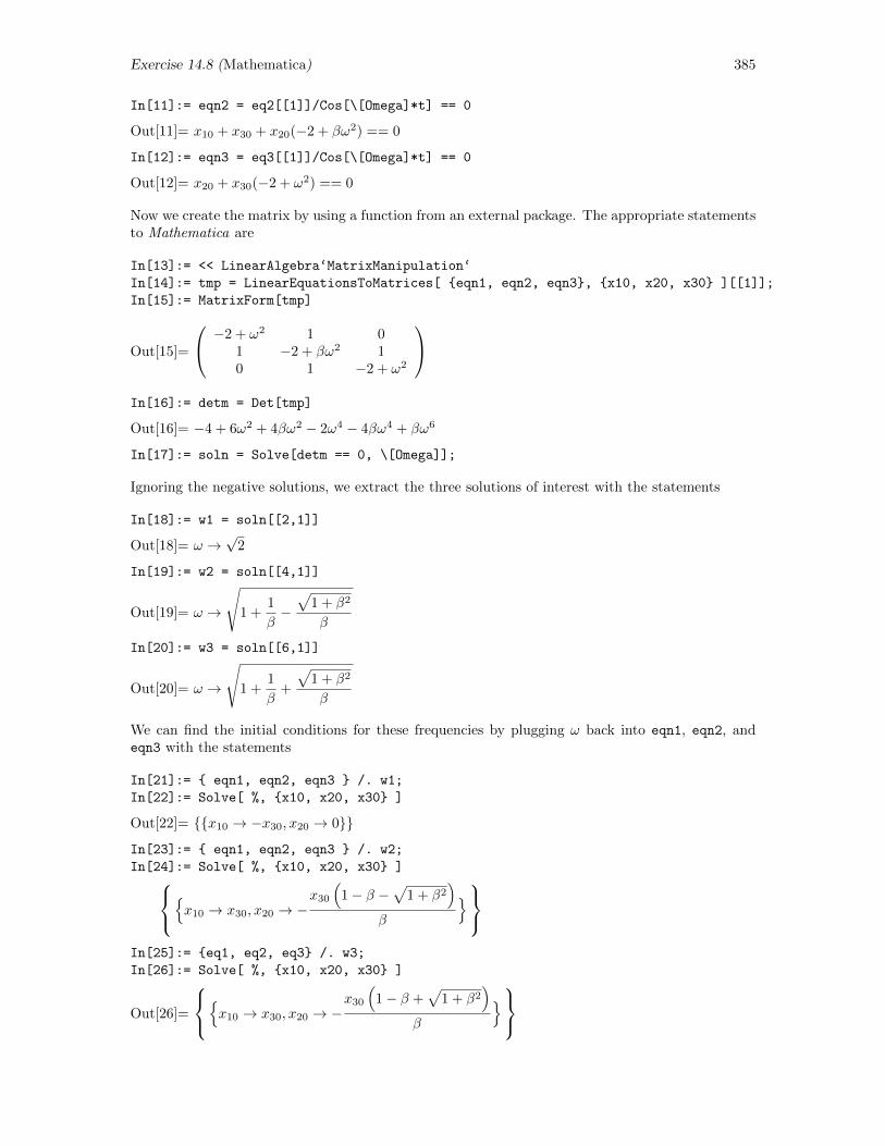
Exercise 14.8 (Mathematica) 385
In[11]:= eqn2 = eq2[[1]]/Cos[\[Omega]*t] == 0
Out[11]= x10 + x30 + x20(−2 + βω2) == 0
In[12]:= eqn3 = eq3[[1]]/Cos[\[Omega]*t] == 0
Out[12]= x20 + x30(−2 + ω2) == 0
Now we create the matrix by using a function from an external package. The appropriate statementsto Mathematica are
In[13]:= << LinearAlgebra‘MatrixManipulation‘
In[14]:= tmp = LinearEquationsToMatrices[ eqn1, eqn2, eqn3, x10, x20, x30 ][[1]];
In[15]:= MatrixForm[tmp]
Out[15]=
−2 + ω2 1 01 −2 + βω2 10 1 −2 + ω2
In[16]:= detm = Det[tmp]
Out[16]= −4 + 6ω2 + 4βω2 − 2ω4 − 4βω4 + βω6
In[17]:= soln = Solve[detm == 0, \[Omega]];
Ignoring the negative solutions, we extract the three solutions of interest with the statements
In[18]:= w1 = soln[[2,1]]
Out[18]= ω →√
2
In[19]:= w2 = soln[[4,1]]
Out[19]= ω →
√1 +
1
β−√
1 + β2
β
In[20]:= w3 = soln[[6,1]]
Out[20]= ω →
√1 +
1
β+
√1 + β2
β
We can find the initial conditions for these frequencies by plugging ω back into eqn1, eqn2, andeqn3 with the statements
In[21]:= eqn1, eqn2, eqn3 /. w1;
In[22]:= Solve[ %, x10, x20, x30 ]
Out[22]= x10 → −x30, x20 → 0
In[23]:= eqn1, eqn2, eqn3 /. w2;
In[24]:= Solve[ %, x10, x20, x30 ]x10 → x30, x20 → −x30
(1− β −
√1 + β2
)β
In[25]:= eq1, eq2, eq3 /. w3;
In[26]:= Solve[ %, x10, x20, x30 ]
Out[26]=
x10 → x30, x20 → −x30
(1− β +
√1 + β2
)β
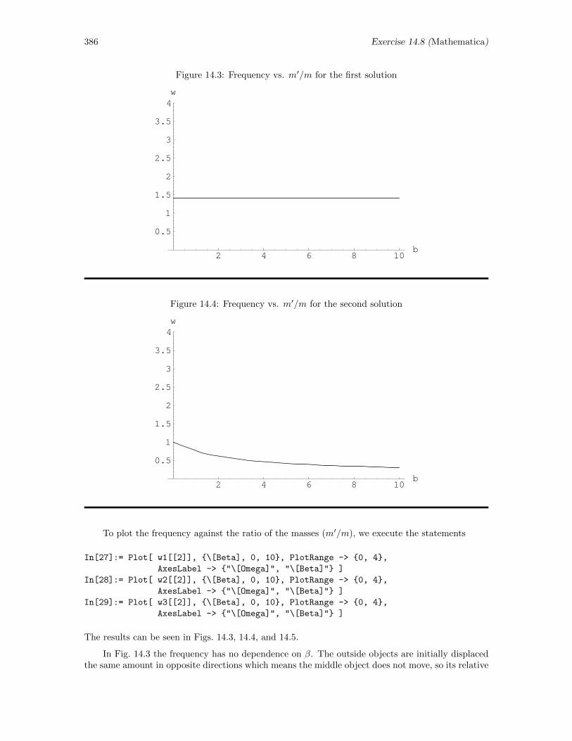
386 Exercise 14.8 (Mathematica)
Figure 14.3: Frequency vs. m′/m for the first solution
2 4 6 8 10b
0.5
1
1.5
2
2.5
3
3.5
4w
Figure 14.4: Frequency vs. m′/m for the second solution
2 4 6 8 10b
0.5
1
1.5
2
2.5
3
3.5
4w
To plot the frequency against the ratio of the masses (m′/m), we execute the statements
In[27]:= Plot[ w1[[2]], \[Beta], 0, 10, PlotRange -> 0, 4,
AxesLabel -> "\[Omega]", "\[Beta]" ]
In[28]:= Plot[ w2[[2]], \[Beta], 0, 10, PlotRange -> 0, 4,
AxesLabel -> "\[Omega]", "\[Beta]" ]
In[29]:= Plot[ w3[[2]], \[Beta], 0, 10, PlotRange -> 0, 4,
AxesLabel -> "\[Omega]", "\[Beta]" ]
The results can be seen in Figs. 14.3, 14.4, and 14.5.
In Fig. 14.3 the frequency has no dependence on β. The outside objects are initially displacedthe same amount in opposite directions which means the middle object does not move, so its relative
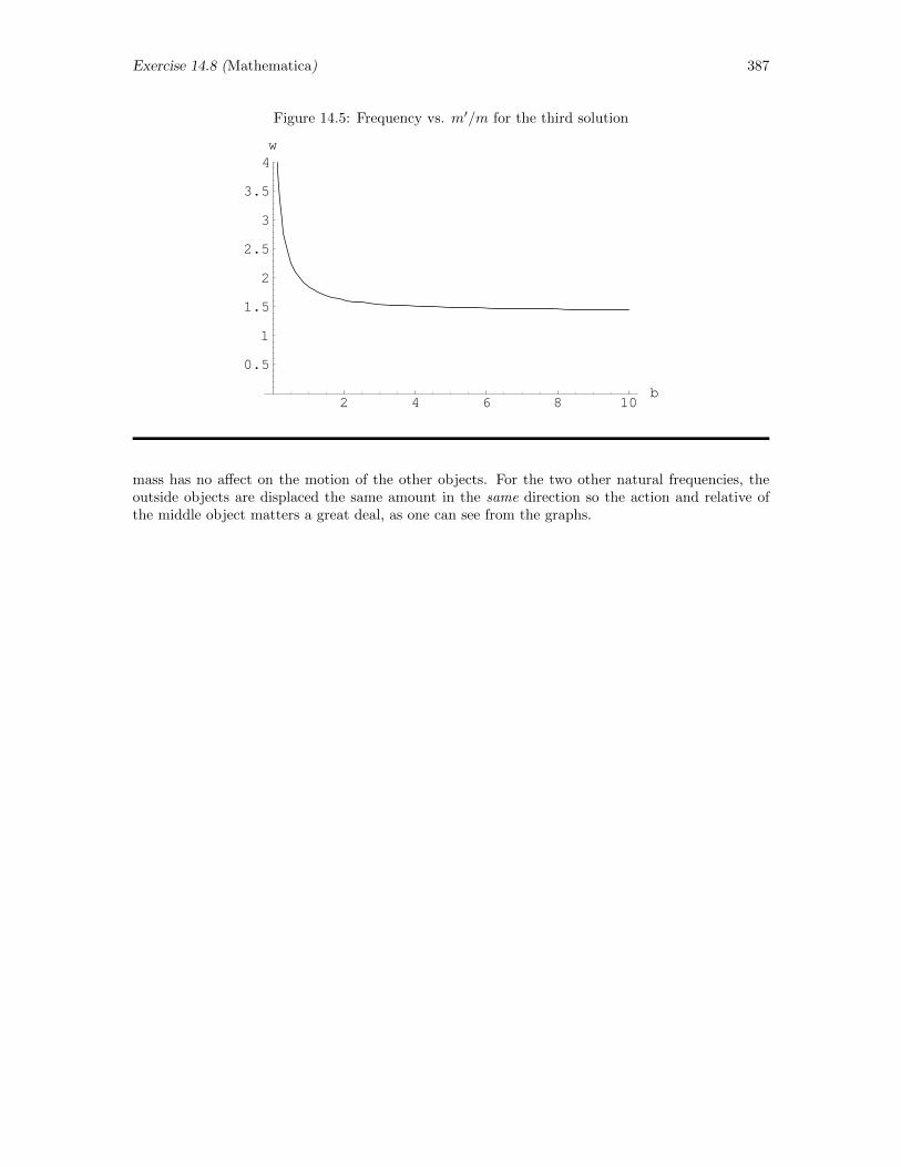
Exercise 14.8 (Mathematica) 387
Figure 14.5: Frequency vs. m′/m for the third solution
2 4 6 8 10b
0.5
1
1.5
2
2.5
3
3.5
4w
mass has no affect on the motion of the other objects. For the two other natural frequencies, theoutside objects are displaced the same amount in the same direction so the action and relative ofthe middle object matters a great deal, as one can see from the graphs.
388 Exercise 14.12 (IDL)
14.12 Square Root by Newton’s Method (IDL)
Exercise: One way to find the square root of a (positive) number a is to find the root of thefunction f(x) = x2−a. (a) Apply Newton’s method symbolically to show that xn+1 = (xn+a/xn)/2.(b) Using a pocket calculator and starting with the guess x0 = 2, work out the first few iteratesby hand and note how quickly this algorithm converges to
√2 = 1.41421. (This algorithm is the
algorithm that most pocket calculators invoke when the square root key is pressed.) (c) Usingwhatever computational tool appeals to you, write a program that asks for the value of a, an initialguess for
√a, and a tolerance and then implements Newton’s method to find
√a, printing out each
iterate along the way and stopping automatically when successive iterates differ by less than thespecified tolerance.
Solution: (a) The square root of a number a can be found by locating the roots of the equationf(x) = x2 − a. With the shorthand notation fn = f(xn) and f ′n = df(x)/dx|xn , we can writeNewton’s method for the function of interest in the form
xn+1 = xn −fnf ′n
= xn −x2n − a2xn
= xn −xn2
+a
2xn=
1
2
(xn +
a
xn
)
(b) With a pocket calculator, if we start with a = 2 and the initial guess x0 = 2, we then find that
x1 =1
2
(x0 +
2
x0
)=
1
2
(2 +
2
2
)= 0.5× 3 = 1.5
Then, the next iteration gives
x2 =1
2
(x1 +
2
x1
)=
1
2
(1.5 +
2
1.5
)= 1.4166667
and the next iteration gives
x3 =1
2
(x2 +
2
x2
)=
1
2
(1.4166667 +
2
1.416667
)= 1.4142157
and the next gives
x4 =1
2
(x3 +
2
x3
)=
1
2
(1.4142157 +
2
1.4142157
)= 1.4142136
The square root of 2 obtained with the square root key on this pocket calculator gives 1.4142136, sofour iterations have apparently given us the square root of 2 to seven digits after the decimal place.
(c) Using basic commands, it is not difficult to construct a program that utilizes Newton’s methodto find the square root of a number. A sample IDL pro-file might contain the statements
;+
;newton.pro
;Batch pro-file newton.pro finds the square root of a number
;specified by the user. The procedure uses an initial guess of
;the square root supplied by the user to start the process and
;then stops when it has reached the desired tolerance which is
;also specified by the user.
;-
READ, a, PROMPT = ’Number whose root is to be found: ’
READ, val, PROMPT = ’Initial Guess: ’
READ, toler, PROMPT = ’Absolute Tolerance: ’
diff = toler + 1.0
Exercise 14.12 (IDL) 389
print, ’Iterative Results’
while diff gt toler do $
begin $
temp = ( val + a/val )/2.0 & $
diff = abs( temp - val ) & $
val = temp & $
print, val & $
endwhile
print, ’Square Root =’ & print, val
(The statement diff = toler + 1.0 is included before the loop to make sure that diff is indeedgreater than toler when the loop is started.) Note that the tolerance is an absolute tolerance andthat each iterate is printed so the user can see how quickly the algorithm converges.
Once this program has been stored in the default directory with the name newton.pro, we canfind the square root of any positive number to any tolerance. For example, to find the square rootof 2, we might run this command file with the statement and input
IDL> @newton
Number whose root is to be found: 2
Initial Guess: 1
Absolute Tolerance: 0.0001
Iterative Results
1.50000
1.41667
1.41422
1.41421
Square Root =
1.41421
A few more sample sessions are shown below. First, we seek the square root of 2 again, butwith a different initial guess, with the “conversation”
IDL> @newton
Number whose root is to be found: 2
Initial Guess: 5
Absolute Tolerance: 0.0001
Iterative Results
2.70000
1.72037
1.44146
1.41447
1.41421
1.41421
Square Root =
1.41421
Next, we seek the square root of 55 with the “conversation”
IDL> @newton
Number whose root is to be found: 55
Initial Guess: 7
Absolute Tolerance: 0.0001
Iterative Results

390 Exercise 14.12 (IDL)
7.42857
7.41621
7.41620
Square Root =
7.41620
In all these examples, convergence to five digits after the decimal point occurs in no more than halfa dozen iterations.
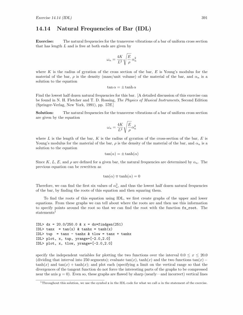
Exercise 14.14 (IDL) 391
14.14 Natural Frequencies of Bar (IDL)
Exercise: The natural frequencies for the transverse vibrations of a bar of uniform cross sectionthat has length L and is free at both ends are given by
ωn =4K
L2
√E
ρα2n
where K is the radius of gyration of the cross section of the bar, E is Young’s modulus for thematerial of the bar, ρ is the density (mass/unit volume) of the material of the bar, and αn is asolution to the equation
tanα = ± tanhα
Find the lowest half dozen natural frequencies for this bar. [A detailed discussion of this exercise canbe found in N. H. Fletcher and T. D. Rossing, The Physics of Musical Instruments, Second Edition(Springer-Verlag, New York, 1991), pp. 57ff.]
Solution: The natural frequencies for the transverse vibrations of a bar of uniform cross sectionare given by the equation
ωn =4K
L2
√E
ρα2n
where L is the length of the bar, K is the radius of gyration of the cross-section of the bar, E isYoung’s modulus for the material of the bar, ρ is the density of the material of the bar, and αn is asolution to the equation
tan(α) = ± tanh(α)
Since K, L, E, and ρ are defined for a given bar, the natural frequencies are determined by αn. Theprevious equation can be rewritten as
tan(α)∓ tanh(α) = 0
Therefore, we can find the first six values of α2n, and thus the lowest half dozen natural frequencies
of the bar, by finding the roots of this equation and then squaring them.
To find the roots of this equation using IDL, we first create graphs of the upper and lowerequations. From these graphs we can tell about where the roots are and then use this informationto specify points around the root so that we can find the root with the function fx_root. Thestatements1
IDL> dx = 20.0/250.0 & x = dx*findgen(251)
IDL> tanx = tan(x) & tanhx = tanh(x)
IDL> tup = tanx - tanhx & tlow = tanx + tanhx
IDL> plot, x, tup, yrange=[-2.0,2.0]
IDL> plot, x, tlow, yrange=[-2.0,2.0]
specify the independent variables for plotting the two functions over the interval 0.0 ≤ x ≤ 20.0(dividing that interval into 250 segments); evaluate tan(x), tanh(x) and the two functions tan(x)−tanh(x) and tan(x) + tanh(x); and plot each (specifying a limit on the vertical range so that thedivergences of the tangent function do not force the interesting parts of the graphs to be compressednear the axis y = 0). Even so, these graphs are flawed by sharp (nearly—and incorrect) vertical lines
1Throughout this solution, we use the symbol x in the IDL code for what we call α in the statement of the exercise.
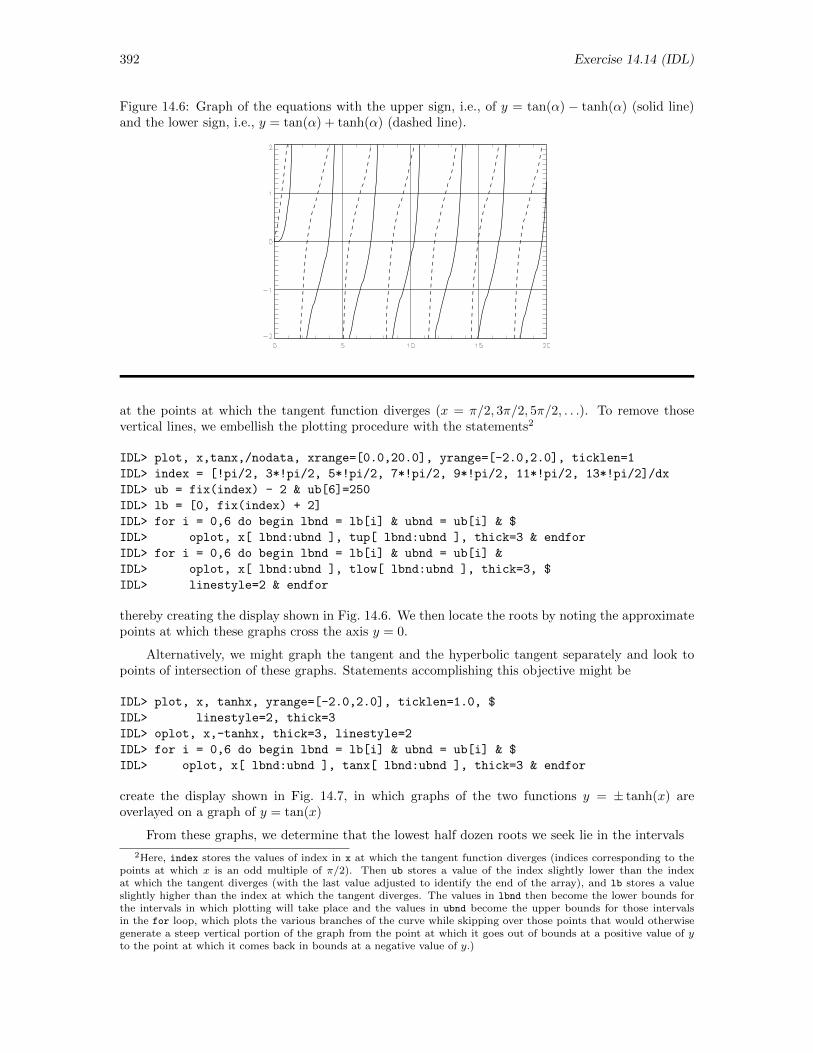
392 Exercise 14.14 (IDL)
Figure 14.6: Graph of the equations with the upper sign, i.e., of y = tan(α) − tanh(α) (solid line)and the lower sign, i.e., y = tan(α) + tanh(α) (dashed line).
at the points at which the tangent function diverges (x = π/2, 3π/2, 5π/2, . . .). To remove thosevertical lines, we embellish the plotting procedure with the statements2
IDL> plot, x,tanx,/nodata, xrange=[0.0,20.0], yrange=[-2.0,2.0], ticklen=1
IDL> index = [!pi/2, 3*!pi/2, 5*!pi/2, 7*!pi/2, 9*!pi/2, 11*!pi/2, 13*!pi/2]/dx
IDL> ub = fix(index) - 2 & ub[6]=250
IDL> lb = [0, fix(index) + 2]
IDL> for i = 0,6 do begin lbnd = lb[i] & ubnd = ub[i] & $
IDL> oplot, x[ lbnd:ubnd ], tup[ lbnd:ubnd ], thick=3 & endfor
IDL> for i = 0,6 do begin lbnd = lb[i] & ubnd = ub[i] &
IDL> oplot, x[ lbnd:ubnd ], tlow[ lbnd:ubnd ], thick=3, $
IDL> linestyle=2 & endfor
thereby creating the display shown in Fig. 14.6. We then locate the roots by noting the approximatepoints at which these graphs cross the axis y = 0.
Alternatively, we might graph the tangent and the hyperbolic tangent separately and look topoints of intersection of these graphs. Statements accomplishing this objective might be
IDL> plot, x, tanhx, yrange=[-2.0,2.0], ticklen=1.0, $
IDL> linestyle=2, thick=3
IDL> oplot, x,-tanhx, thick=3, linestyle=2
IDL> for i = 0,6 do begin lbnd = lb[i] & ubnd = ub[i] & $
IDL> oplot, x[ lbnd:ubnd ], tanx[ lbnd:ubnd ], thick=3 & endfor
create the display shown in Fig. 14.7, in which graphs of the two functions y = ± tanh(x) areoverlayed on a graph of y = tan(x)
From these graphs, we determine that the lowest half dozen roots we seek lie in the intervals
2Here, index stores the values of index in x at which the tangent function diverges (indices corresponding to thepoints at which x is an odd multiple of π/2). Then ub stores a value of the index slightly lower than the indexat which the tangent diverges (with the last value adjusted to identify the end of the array), and lb stores a valueslightly higher than the index at which the tangent diverges. The values in lbnd then become the lower bounds forthe intervals in which plotting will take place and the values in ubnd become the upper bounds for those intervalsin the for loop, which plots the various branches of the curve while skipping over those points that would otherwisegenerate a steep vertical portion of the graph from the point at which it goes out of bounds at a positive value of yto the point at which it comes back in bounds at a negative value of y.)
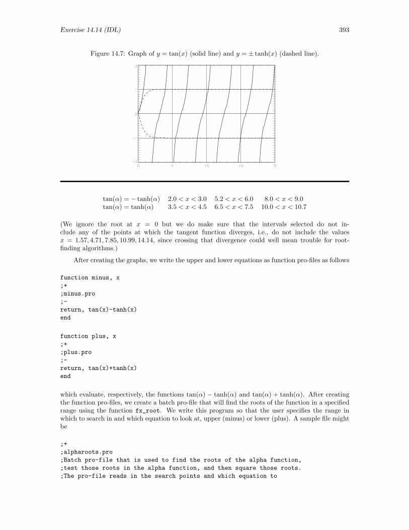
Exercise 14.14 (IDL) 393
Figure 14.7: Graph of y = tan(x) (solid line) and y = ± tanh(x) (dashed line).
tan(α) = − tanh(α) 2.0 < x < 3.0 5.2 < x < 6.0 8.0 < x < 9.0tan(α) = tanh(α) 3.5 < x < 4.5 6.5 < x < 7.5 10.0 < x < 10.7
(We ignore the root at x = 0 but we do make sure that the intervals selected do not in-clude any of the points at which the tangent function diverges, i.e., do not include the valuesx = 1.57, 4.71, 7.85, 10.99, 14.14, since crossing that divergence could well mean trouble for root-finding algorithms.)
After creating the graphs, we write the upper and lower equations as function pro-files as follows
function minus, x
;+
;minus.pro
;-
return, tan(x)-tanh(x)
end
function plus, x
;+
;plus.pro
;-
return, tan(x)+tanh(x)
end
which evaluate, respectively, the functions tan(α) − tanh(α) and tan(α) + tanh(α). After creatingthe function pro-files, we create a batch pro-file that will find the roots of the function in a specifiedrange using the function fx_root. We write this program so that the user specifies the range inwhich to search in and which equation to look at, upper (minus) or lower (plus). A sample file mightbe
;+
;alpharoots.pro
;Batch pro-file that is used to find the roots of the alpha function,
;test those roots in the alpha function, and then square those roots.
;The pro-file reads in the search points and which equation to
394 Exercise 14.14 (IDL)
;search from the user. Then, the function fx_root is used to find the
;root using the information supplied by the user.
;-
READ, a, PROMPT = ’Provide a low guess for the root : ’
READ, b, PROMPT = ’Provide a middle guess for the root: ’
READ, c, PROMPT = ’Provide an upper guess for the root: ’
name = ’’
READ, name, PROMPT = ’minus or plus solution: ’
searchpoints = [a, b, c]
root = fx_root(searchpoints, name)
root= float(root)
print, ’Root = ’ & print, root
trial = call_function(name, root)
print, ’Alpha at Root = ’ & print, trial
sqr = root^2
print, ’Root^2= ’ & print, sqr
After creating this batch pro-file we can easily find the six lowest roots of the alpha equation. Tofind the first root in the equation with the upper sign (and save the square of the root), we executethe statements
IDL> @alpharoots
Provide a low guess for the root : 2.0
Provide a middle guess for the root: 2.5
Provide an upper guess for the root: 3.0
minus or plus solution: plus
Root = 2.36502
Alpha at Root = -1.78814e-07
Root^2= 5.59332
IDL> rtsq = fltarr(6) ; Prepare array to save roots
IDL> rtsq[0] = sqr
Further sessions to find the other roots involve the statements
IDL> @alpharoots
Provide a low guess for the root : 5.2
Provide a middle guess for the root: 5.5
Provide an upper guess for the root: 6.0
minus or plus solution: plus
Root = 5.49780
Alpha at Root = 4.76837e-07
Root^2= 30.2259
IDL> rtsq[2] = sqr
IDL> @alpharoots
Provide a low guess for the root : 8.0
Provide a middle guess for the root: 8.5
Provide an upper guess for the root: 9.0
minus or plus solution: plus
Root = 8.63938
Alpha at Root = -6.55651e-07
Root^2= 74.6389
IDL> rtsq[4] = sqr
Exercise 14.14 (IDL) 395
IDL> @alpharoots
Provide a low guess for the root : 3.5
Provide a middle guess for the root: 4.0
Provide an upper guess for the root: 4.5
minus or plus solution: minus
Root = 3.92660
Alpha at Root = 1.19209e-07
Root^2= 15.4182
IDL> rtsq[1] = sqr
IDL> @alpharoots
Provide a low guess for the root : 6.5
Provide a middle guess for the root: 7.0
Provide an upper guess for the root: 7.5
minus or plus solution: minus
Root = 7.06858
Alpha at Root = -4.17233e-07
Root^2= 49.9649
IDL> rtsq[3] = sqr
IDL> @alpharoots
Provide a low guess for the root : 10.0
Provide a middle guess for the root: 10.4
Provide an upper guess for the root: 10.7
minus or plus solution: minus
Root = 10.2102
Alpha at Root = 7.15256e-07
Root^2= 104.248
IDL> rtsq[5] = sqr
Next, let us display the values of the squared roots, both in absolute terms and as multiples ofthe lowest frequency, with the statements
IDL> print, rtsq
5.59332 15.4182 30.2259 49.9649 74.6389 104.248
IDL> print, rtsq/rtsq[0]
1.00000 2.75654 5.40392 8.93295 13.3443 18.6379
Note in particular that the frequencies at which this bar oscillates are not integer multiples of thelowest (fundamental) frequency.
Similar program can be created that use a different root finding function. For example if wewanted to use the function newton to find the roots, then the program would be
;+
;alphanewt.pro
;Batch pro-file that is used to find the roots of the alpha function
;and then test those roots in the alpha function. The pro-file reads in
;a point from which to start the search and which equation to search
;from the user. Then, the newton function is used to find the
;root using the starting point specified by the user.
;-
READ, a, PROMPT = ’Provide a starting point: ’
name = ’’
READ, name, PROMPT = ’minus or plus solution: ’
396 Exercise 14.14 (IDL)
root =newton(a, name)
root= float(root)
print, ’Root = ’ & print, root
trial = call_function(name, root)
print, ’Alpha at Root = ’ & print, trial
sqr = root^2
print, ’Root^2 = ’ & print, sqr
and a sample run would have the form
IDL> @alphanewt
IDL> @alphanewt
Provide a starting point: 2.0
minus or plus solution: plus
Root = 2.36502
Alpha at Root = -6.55651e-07
Root^2= 5.59332
From these sessions we can see that the the values of α2n that correspond to the lowest six
natural frequencies are 5.59332, 15.4182, 30.2259, 49.9649, 74.6389, and 104.248. Thus, the lowesthalf dozen natural frequencies of this bar are
ω1 = 5.593324K
L2
√E
ρω2 = 15.4182
4K
L2
√E
ρ= 2.75654ω1
ω3 = 30.22594K
L2
√E
ρ= 5.40392ω1 ω4 = 49.9649
4K
L2
√E
ρ= 8.93295ω1
ω5 = 74.63894K
L2
√E
ρ= 13.3443ω1 ω6 = 104.248
4K
L2
√E
ρ= 18.6379ω1
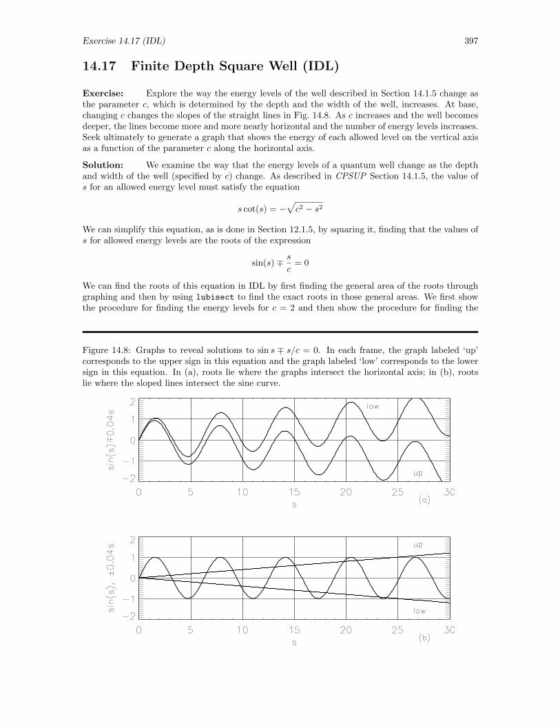
Exercise 14.17 (IDL) 397
14.17 Finite Depth Square Well (IDL)
Exercise: Explore the way the energy levels of the well described in Section 14.1.5 change asthe parameter c, which is determined by the depth and the width of the well, increases. At base,changing c changes the slopes of the straight lines in Fig. 14.8. As c increases and the well becomesdeeper, the lines become more and more nearly horizontal and the number of energy levels increases.Seek ultimately to generate a graph that shows the energy of each allowed level on the vertical axisas a function of the parameter c along the horizontal axis.
Solution: We examine the way that the energy levels of a quantum well change as the depthand width of the well (specified by c) change. As described in CPSUP Section 14.1.5, the value ofs for an allowed energy level must satisfy the equation
s cot(s) = −√c2 − s2
We can simplify this equation, as is done in Section 12.1.5, by squaring it, finding that the values ofs for allowed energy levels are the roots of the expression
sin(s)∓ s
c= 0
We can find the roots of this equation in IDL by first finding the general area of the roots throughgraphing and then by using lubisect to find the exact roots in those general areas. We first showthe procedure for finding the energy levels for c = 2 and then show the procedure for finding the
Figure 14.8: Graphs to reveal solutions to sin s ∓ s/c = 0. In each frame, the graph labeled ‘up’corresponds to the upper sign in this equation and the graph labeled ‘low’ corresponds to the lowersign in this equation. In (a), roots lie where the graphs intersect the horizontal axis; in (b), rootslie where the sloped lines intersect the sine curve.
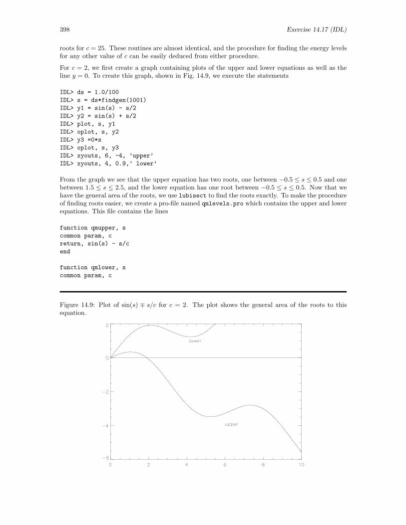
398 Exercise 14.17 (IDL)
roots for c = 25. These routines are almost identical, and the procedure for finding the energy levelsfor any other value of c can be easily deduced from either procedure.
For c = 2, we first create a graph containing plots of the upper and lower equations as well as theline y = 0. To create this graph, shown in Fig. 14.9, we execute the statements
IDL> ds = 1.0/100
IDL> s = ds*findgen(1001)
IDL> y1 = sin(s) - s/2
IDL> y2 = sin(s) + s/2
IDL> plot, s, y1
IDL> oplot, s, y2
IDL> y3 =0*s
IDL> oplot, s, y3
IDL> xyouts, 6, -4, ’upper’
IDL> xyouts, 4, 0.9,’ lower’
From the graph we see that the upper equation has two roots, one between −0.5 ≤ s ≤ 0.5 and onebetween 1.5 ≤ s ≤ 2.5, and the lower equation has one root between −0.5 ≤ s ≤ 0.5. Now that wehave the general area of the roots, we use lubisect to find the roots exactly. To make the procedureof finding roots easier, we create a pro-file named qmlevels.pro which contains the upper and lowerequations. This file contains the lines
function qmupper, s
common param, c
return, sin(s) - s/c
end
function qmlower, s
common param, c
Figure 14.9: Plot of sin(s) ∓ s/c for c = 2. The plot shows the general area of the roots to thisequation.
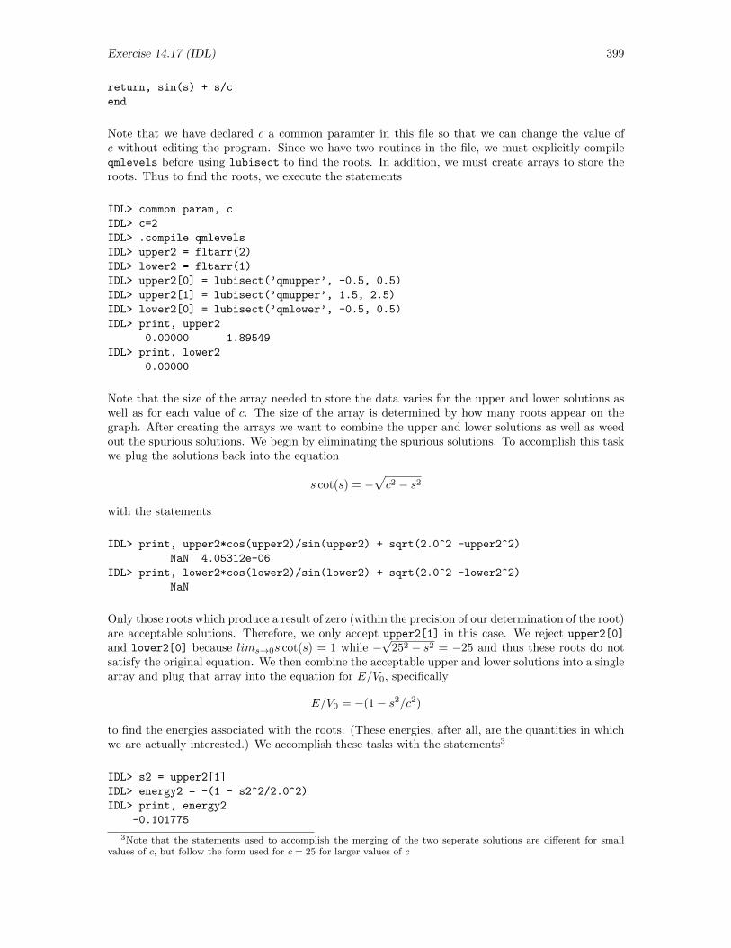
Exercise 14.17 (IDL) 399
return, sin(s) + s/c
end
Note that we have declared c a common paramter in this file so that we can change the value ofc without editing the program. Since we have two routines in the file, we must explicitly compileqmlevels before using lubisect to find the roots. In addition, we must create arrays to store theroots. Thus to find the roots, we execute the statements
IDL> common param, c
IDL> c=2
IDL> .compile qmlevels
IDL> upper2 = fltarr(2)
IDL> lower2 = fltarr(1)
IDL> upper2[0] = lubisect(’qmupper’, -0.5, 0.5)
IDL> upper2[1] = lubisect(’qmupper’, 1.5, 2.5)
IDL> lower2[0] = lubisect(’qmlower’, -0.5, 0.5)
IDL> print, upper2
0.00000 1.89549
IDL> print, lower2
0.00000
Note that the size of the array needed to store the data varies for the upper and lower solutions aswell as for each value of c. The size of the array is determined by how many roots appear on thegraph. After creating the arrays we want to combine the upper and lower solutions as well as weedout the spurious solutions. We begin by eliminating the spurious solutions. To accomplish this taskwe plug the solutions back into the equation
s cot(s) = −√c2 − s2
with the statements
IDL> print, upper2*cos(upper2)/sin(upper2) + sqrt(2.0^2 -upper2^2)
NaN 4.05312e-06
IDL> print, lower2*cos(lower2)/sin(lower2) + sqrt(2.0^2 -lower2^2)
NaN
Only those roots which produce a result of zero (within the precision of our determination of the root)are acceptable solutions. Therefore, we only accept upper2[1] in this case. We reject upper2[0]
and lower2[0] because lims→0s cot(s) = 1 while −√
252 − s2 = −25 and thus these roots do notsatisfy the original equation. We then combine the acceptable upper and lower solutions into a singlearray and plug that array into the equation for E/V0, specifically
E/V0 = −(1− s2/c2)
to find the energies associated with the roots. (These energies, after all, are the quantities in whichwe are actually interested.) We accomplish these tasks with the statements3
IDL> s2 = upper2[1]
IDL> energy2 = -(1 - s2^2/2.0^2)
IDL> print, energy2
-0.101775
3Note that the statements used to accomplish the merging of the two seperate solutions are different for smallvalues of c, but follow the form used for c = 25 for larger values of c
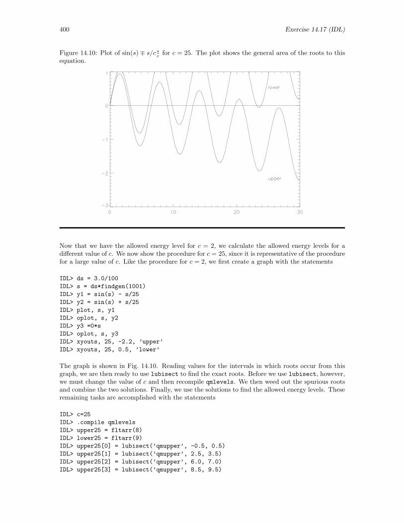
400 Exercise 14.17 (IDL)
Figure 14.10: Plot of sin(s)∓ s/c sc for c = 25. The plot shows the general area of the roots to thisequation.
Now that we have the allowed energy level for c = 2, we calculate the allowed energy levels for adifferent value of c. We now show the procedure for c = 25, since it is representative of the procedurefor a large value of c. Like the procedure for c = 2, we first create a graph with the statements
IDL> ds = 3.0/100
IDL> s = ds*findgen(1001)
IDL> y1 = sin(s) - s/25
IDL> y2 = sin(s) + s/25
IDL> plot, s, y1
IDL> oplot, s, y2
IDL> y3 =0*s
IDL> oplot, s, y3
IDL> xyouts, 25, -2.2, ’upper’
IDL> xyouts, 25, 0.5, ’lower’
The graph is shown in Fig. 14.10. Reading values for the intervals in which roots occur from thisgraph, we are then ready to use lubisect to find the exact roots. Before we use lubisect, however,we must change the value of c and then recompile qmlevels. We then weed out the spurious rootsand combine the two solutions. Finally, we use the solutions to find the allowed energy levels. Theseremaining tasks are accomplished with the statements
IDL> c=25
IDL> .compile qmlevels
IDL> upper25 = fltarr(8)
IDL> lower25 = fltarr(9)
IDL> upper25[0] = lubisect(’qmupper’, -0.5, 0.5)
IDL> upper25[1] = lubisect(’qmupper’, 2.5, 3.5)
IDL> upper25[2] = lubisect(’qmupper’, 6.0, 7.0)
IDL> upper25[3] = lubisect(’qmupper’, 8.5, 9.5)
Exercise 14.17 (IDL) 401
IDL> upper25[4] = lubisect(’qmupper’, 12.5, 13.5)
IDL> upper25[5] = lubisect(’qmupper’, 14.5, 15.5)
IDL> upper25[6] = lubisect(’qmupper’, 19,0, 20.0)
IDL> upper25[7] = lubisect(’qmupper’, 20.5, 21.5)
IDL> lower25[0] = lubisect(’qmlower’, -0.5, 0.5)
IDL> lower25[1] = lubisect(’qmlower’, 3.0, 4.0)
IDL> lower25[2] = lubisect(’qmlower’, 5.5, 6.5)
IDL> lower25[3] = lubisect(’qmlower’, 9.5, 10.5)
IDL> lower25[4] = lubisect(’qmlower’, 11.5, 12.5)
IDL> lower25[5] = lubisect(’qmlower’, 16.0, 17.0)
IDL> lower25[6] = lubisect(’qmlower’, 17.5, 18.5)
IDL> lower25[7] = lubisect(’qmlower’, 22.5, 23.5)
IDL> lower25[8] = lubisect(’qmlower’, 23.5, 24.5)
IDL> print, upper25
-1.00000e-06 3.02048 6.54820 9.05419 13.1188 15.0614
19.7611 20.9943
IDL> print, upper25*cos(upper25)/sin(upper25) + sqrt(25.0^2 -upper25^2)
NaN -7.43866e-05 48.2544 -3.81470e-06 42.5628 -3.24249e-05
30.6268 -3.52859e-05
IDL> print, lower25
-1.00000e-06 3.27289 6.03920 9.82884 12.0628 16.4248
18.0433 23.1778 23.8645
IDL> print, lower25*cos(lower25)/sin(lower25) + sqrt(25.0^2 -lower25^2)
NaN 49.5695 -4.00543e-05 45.9736 4.95911e-05 37.6949
9.53674e-06 18.7393 1.81198e-05
IDL> s25 = lower25[1:8]
IDL> for i= 1, 7, 2 do s25[i-1] = upper25[i]
IDL> print, s25
3.02048 6.03920 9.05419 12.0628 15.0614 18.0433
20.9943 23.8645
IDL> energy25 = -(1- s^2/25.0^2)
IDL> print, energy25
-0.985403 -0.941645 -0.868835 -0.767180 -0.637047 -0.479105
-0.294784 -0.0887774
After finding the allowed energy levels for c = 25, we use similar procedures to find the allowedenergy levels for other values of c. Once we have found the allowed energy levels for a variety of cvalues, we plot a diagram that shows the allowed energy levels for different values of c. In our casewe choose 2, 5, 20, 25 and 50 as our values of c. To create the plot we use the statements
IDL> plot, [-0.5, 5.5], [0.5, -1.5], /nodata, xstyle=4, ystyle=4
IDL> axis, 0.0, yaxis= 0, ytitle=’E/V!DO!N’, charsize=1.5
IDL> oplot, [0.2, 0.8], [energy2[0], energy2[0]], thick=3.0
IDL> for i=0,1 do oplot, [1.2, 1.8],[energy5[i], energy5[i]], thick=3.0
IDL> for i=0,2 do oplot, [2.2, 2.8],[energy10[i], energy10[i]], thick=3.0
IDL> for i=0,7 do oplot, [3.2, 3.8],[energy25[i], energy25[i]], thick=3.0
IDL> for i=0,15 do oplot, [4.2, 4.8],[energy50[i], energy50[i]], thick=3.0
IDL> oplot, [0.0,5.2,5.2,5.5], [-1.0,-1.0,0.0,0.0]
IDL> xyouts, 0.4, -1.1, ’2’
IDL> xyouts, 1.4, -1.1, ’5’
IDL> xyouts, 2.35, -1.1, ’10’
IDL> xyouts, 3.35, -1.1, ’25’
IDL> xyouts, 4.35, -1.1, ’50’
The resulting graph is shown in Fig. 14.11. From this diagram, we see that the number of allowed
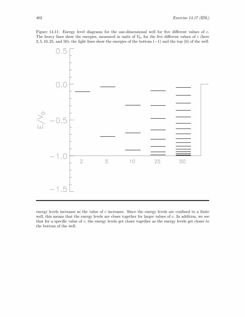
402 Exercise 14.17 (IDL)
Figure 14.11: Energy level diagrams for the one-dimensional well for five different values of c.The heavy lines show the energies, measured in units of V0, for the five different values of c (here2, 5, 10, 25, and 50); the light lines show the energies of the bottom (−1) and the top (0) of the well.
energy levels increases as the value of c increases. Since the energy levels are confined to a finitewell, this means that the energy levels are closer together for larger values of c. In addition, we seethat for a specific value of c, the energy levels get closer together as the energy levels get closer tothe bottom of the well.
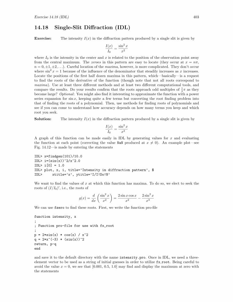
Exercise 14.18 (IDL) 403
14.18 Single-Slit Diffraction (IDL)
Exercise: The intensity I(x) in the diffraction pattern produced by a single slit is given by
I(x)
I0=
sin2 x
x2
where I0 is the intensity in the center and x is related to the position of the observation point awayfrom the central maximum. The zeroes in this pattern are easy to locate (they occur at x = nπ,n = 0,±1,±2, . . .). Careful location of the maxima, however, is more complicated. They don’t occurwhere sin2 x = 1 because of the influence of the denominator that steadily increases as x increases.Locate the positions of the first half dozen maxima in this pattern, which—basically—is a requestto find the roots of the derivative of the function (though note that not all roots correspond tomaxima). Use at least three different methods and at least two different computational tools, andcompare the results. Do your results confirm that the roots approach odd multiples of 1
2π as theybecome large? Optional : You might also find it interesting to approximate the function with a powerseries expansion for sinx, keeping quite a few terms but converting the root finding problem intothat of finding the roots of a polynomial. Then, use methods for finding roots of polynomials andsee if you can come to understand how accuracy depends on how many terms you keep and whichroot you seek.
Solution: The intensity I(x) in the diffraction pattern produced by a single slit is given by
I(x)
I0=
sin2 x
x2
A graph of this function can be made easily in IDL by generating values for x and evaluatingthe function at each point (correcting the value NaN produced at x 6= 0). An example plot—seeFig. 14.12—is made by entering the statements
IDL> x=findgen(101)/10.0
IDL> i=(sin(x))^2/x^2.0
IDL> i[0] = 1.0
IDL> plot, x, i, title=’Intensity in diffraction pattern’, $
IDL> xtitle=’x’, ytitle=’I/I!Do!N’
We want to find the values of x at which this function has maxima. To do so, we elect to seek theroots of (I/I0)′, i.e., the roots of
g(x) =d
dx
(sin2 x
x2
)=
2 sinx cosx
x2− 2 sin2 x
x3
We can use fzero to find these roots. First, we write the function pro-file
function intensity, x
;
; Function pro-file for use with fx_root
;
p = 2*sin(x) * cos(x) / x^2
q = 2*x^(-3) * (sin(x))^2
return, p-q
end
and save it to the default directory with the name intensity.pro. Once in IDL, we need a three-element vector to be used as a string of initial guesses in order to utilize fx root. Being careful toavoid the value x = 0, we see that [0.001, 0.5, 1.0] may find and display the maximum at zero withthe statements
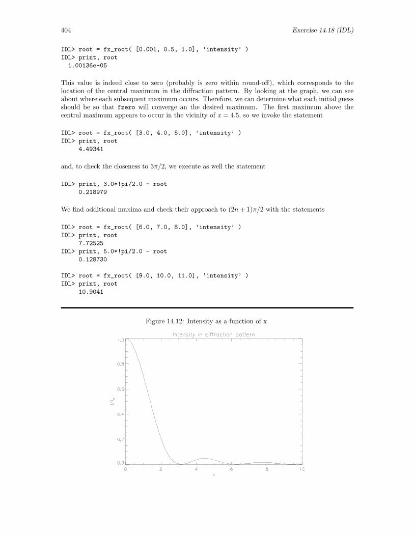
404 Exercise 14.18 (IDL)
IDL> root = fx_root( [0.001, 0.5, 1.0], ’intensity’ )
IDL> print, root
1.00136e-05
This value is indeed close to zero (probably is zero within round-off), which corresponds to thelocation of the central maximum in the diffraction pattern. By looking at the graph, we can seeabout where each subsequent maximum occurs. Therefore, we can determine what each initial guessshould be so that fzero will converge an the desired maximum. The first maximum above thecentral maximum appears to occur in the vicinity of x = 4.5, so we invoke the statement
IDL> root = fx_root( [3.0, 4.0, 5.0], ’intensity’ )
IDL> print, root
4.49341
and, to check the closeness to 3π/2, we execute as well the statement
IDL> print, 3.0*!pi/2.0 - root
0.218979
We find additional maxima and check their approach to (2n+ 1)π/2 with the statements
IDL> root = fx_root( [6.0, 7.0, 8.0], ’intensity’ )
IDL> print, root
7.72525
IDL> print, 5.0*!pi/2.0 - root
0.128730
IDL> root = fx_root( [9.0, 10.0, 11.0], ’intensity’ )
IDL> print, root
10.9041
Figure 14.12: Intensity as a function of x.
Exercise 14.18 (IDL) 405
IDL> print, 7.0*!pi/2.0 - root
0.0914536
IDL> root = fx_root( [12.0,13.0,14.0], ’intensity’ )
IDL> print, root
14.0662
IDL> print, 9.0*!pi/2.0 - root
0.0709734
IDL> root = fx_root( [15.0, 16.0, 17.0], ’intensity’ )
IDL> print, root
17.2208
IDL> print, 11.0*!pi/2.0 - root
0.0580063
By looking at the roots and the comparisons that follow, we see that the maxima are found at x ≈ 0,3π/2, 5π/2, 7π/2, etc. Furthermore, we see that the difference between the root and the multipleof π/2 lessens as the size of the root increases. So, the maxima do indeed approach odd multiplesof π/2 as the roots become large.
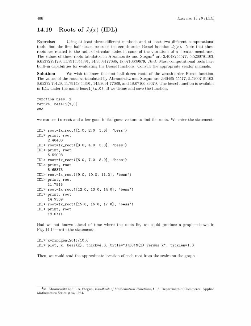
406 Exercise 14.19 (IDL)
14.19 Roots of J0(x) (IDL)
Exercise: Using at least three different methods and at least two different computationaltools, find the first half dozen roots of the zeroth-order Bessel function J0(x). Note that theseroots are related to the radii of circular nodes in some of the vibrations of a circular membrane.The values of these roots tabulated in Abramowitz and Stegun4 are 2.4048255577, 5.5200781103,8.6537279129, 11.7915344391, 14.9309177086, 18.0710639679. Hint : Most computational tools havebuilt-in capabilities for evaluating the Bessel functions. Consult the appropriate vendor manuals.
Solution: We wish to know the first half dozen roots of the zeroth-order Bessel function.The values of the roots as tabulated by Abramowitz and Stegun are 2.40485 55577, 5.52007 81103,8.65372 79129, 11.79153 44391, 14.93091 77086, and 18.07106 39679. The bessel function is availablein IDL under the name beselj(x,0). If we define and save the function,
function bess, x
return, beselj(x,0)
end
we can use fx root and a few good initial guess vectors to find the roots. We enter the statements
IDL> root=fx_root([1.0, 2.0, 3.0], ’bess’)
IDL> print, root
2.40483
IDL> root=fx_root([3.0, 4.0, 5.0], ’bess’)
IDL> print, root
5.52008
IDL> root=fx_root([6.0, 7.0, 8.0], ’bess’)
IDL> print, root
8.65373
IDL> root=fx_root([9.0, 10.0, 11.0], ’bess’)
IDL> print, root
11.7915
IDL> root=fx_root([12.0, 13.0, 14.0], ’bess’)
IDL> print, root
14.9309
IDL> root=fx_root([15.0, 16.0, 17.0], ’bess’)
IDL> print, root
18.0711
Had we not known ahead of time where the roots lie, we could produce a graph—shown inFig. 14.13—with the statements
IDL> x=findgen(201)/10.0
IDL> plot, x, bess(x), thick=4.0, title="J!D0!N(x) versus x", ticklen=1.0
Then, we could read the approximate location of each root from the scales on the graph.
4M. Abramowitz and I. A. Stegun, Handbook of Mathematical Functions, U. S. Department of Commerce, AppliedMathematics Series #55, 1964.
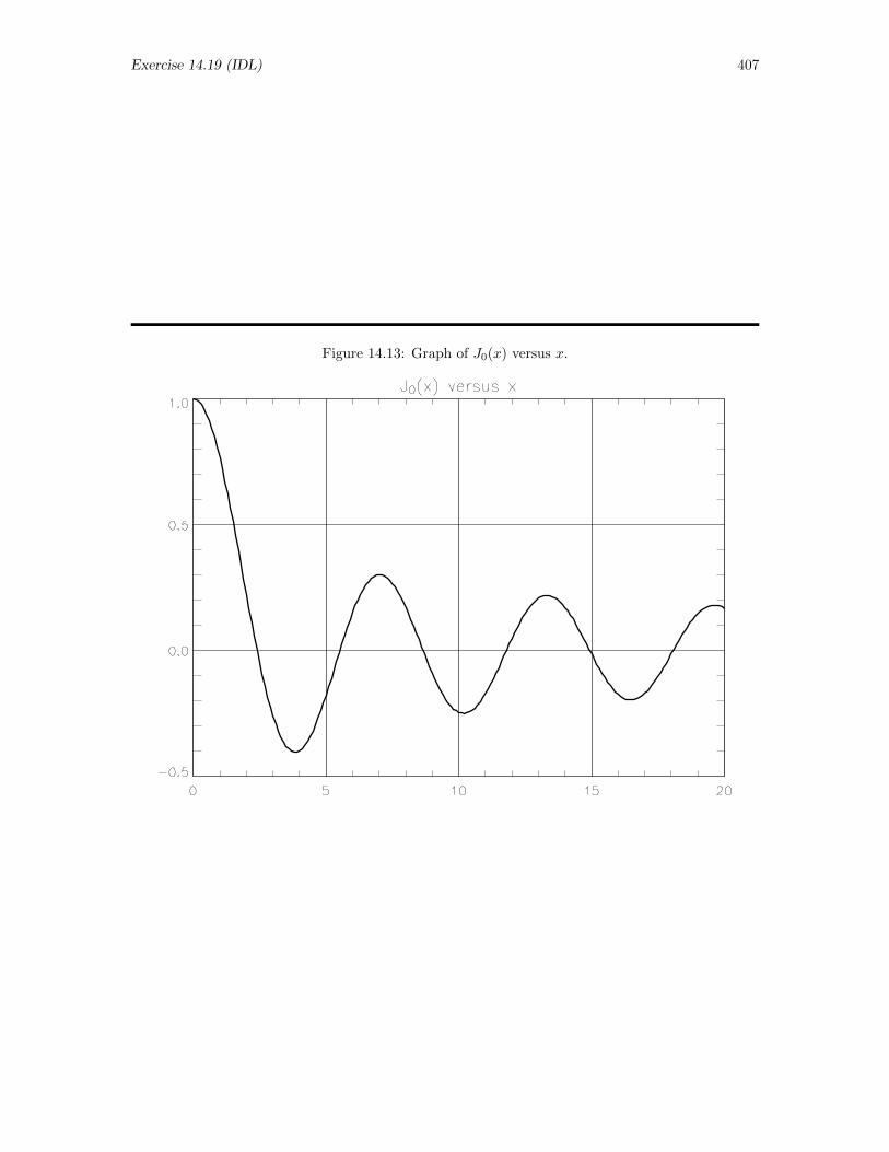
Exercise 14.19 (IDL) 407
Figure 14.13: Graph of J0(x) versus x.
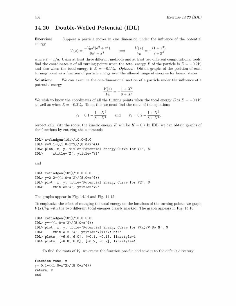
408 Exercise 14.20 (IDL)
14.20 Double-Welled Potential (IDL)
Exercise: Suppose a particle moves in one dimension under the influence of the potentialenergy
V (x) =−V0a
2(a2 + x2)
8a4 + x4=⇒ V (x)
V0= − (1 + x2)
8 + x4
where x = x/a. Using at least three different methods and at least two different computational tools,find the coordinates x of all turning points when the total energy E of the particle is E = −0.2V0
and also when the total energy is E = −0.1V0. Optional : Obtain graphs of the position of eachturning point as a function of particle energy over the allowed range of energies for bound states.
Solution: We can examine the one-dimensional motion of a particle under the influence of apotential energy
V (x)
V0= −1 +X2
8 +X4
We wish to know the coordinates of all the turning points when the total energy E is E = −0.1V0
as well as when E = −0.2V0. To do this we must find the roots of the equations
V1 = 0.1− 1 +X2
8 +X4and V2 = 0.2− 1 +X2
8 +X4,
respectively. (At the roots, the kinetic energy K will be K = 0.) In IDL, we can obtain graphs ofthe functions by entering the commands
IDL> x=findgen(101)/10.0-5.0
IDL> y=0.1-((1.0+x^2)/(8.0+x^4))
IDL> plot, x, y, title=’Potential Energy Curve for V1’, $
IDL> xtitle=’X’, ytitle=’V1’
and
IDL> x=findgen(101)/10.0-5.0
IDL> y=0.2-((1.0+x^2)/(8.0+x^4))
IDL> plot, x, y, title=’Potential Energy Curve for V2’, $
IDL> xtitle=’X’, ytitle=’V2’
The graphs appear in Fig. 14.14 and Fig. 14.15.
To emphasize the effect of changing the total energy on the locations of the turning points, we graphV (x)/V0 with the two different total energies clearly marked. The graph appears in Fig. 14.16.
IDL> x=findgen(101)/10.0-5.0
IDL> y=-((1.0+x^2)/(8.0+x^4))
IDL> plot, x, y, title=’Potential Energy Curve for V(x)/V!Do!N’, $
IDL> xtitle = ’X’, ytitle=’V(x)/V!Do!N’
IDL> plots, [-6.0, 6.0], [-0.1, -0.1], linestyle=1
IDL> plots, [-6.0, 6.0], [-0.2, -0.2], linestyle=1
To find the roots of V1, we create the function pro-file and save it to the default directory.
function vone, x
y= 0.1-((1.0+x^2)/(8.0+x^4))
return, y
end
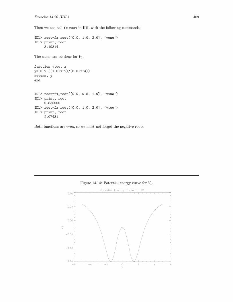
Exercise 14.20 (IDL) 409
Then we can call fx root in IDL with the following commands:
IDL> root=fx_root([0.0, 1.0, 2.0], ’vone’)
IDL> print, root
3.19314
The same can be done for V2.
function vtwo, x
y= 0.2-((1.0+x^2)/(8.0+x^4))
return, y
end
IDL> root=fx_root([0.0, 0.5, 1.0], ’vtwo’)
IDL> print, root
0.835000
IDL> root=fx_root([0.0, 1.0, 2.0], ’vtwo’)
IDL> print, root
2.07431
Both functions are even, so we must not forget the negative roots.
Figure 14.14: Potential energy curve for V1.
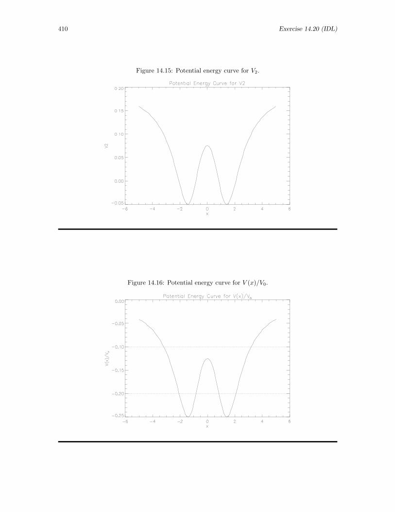
410 Exercise 14.20 (IDL)
Figure 14.15: Potential energy curve for V2.
Figure 14.16: Potential energy curve for V (x)/V0.
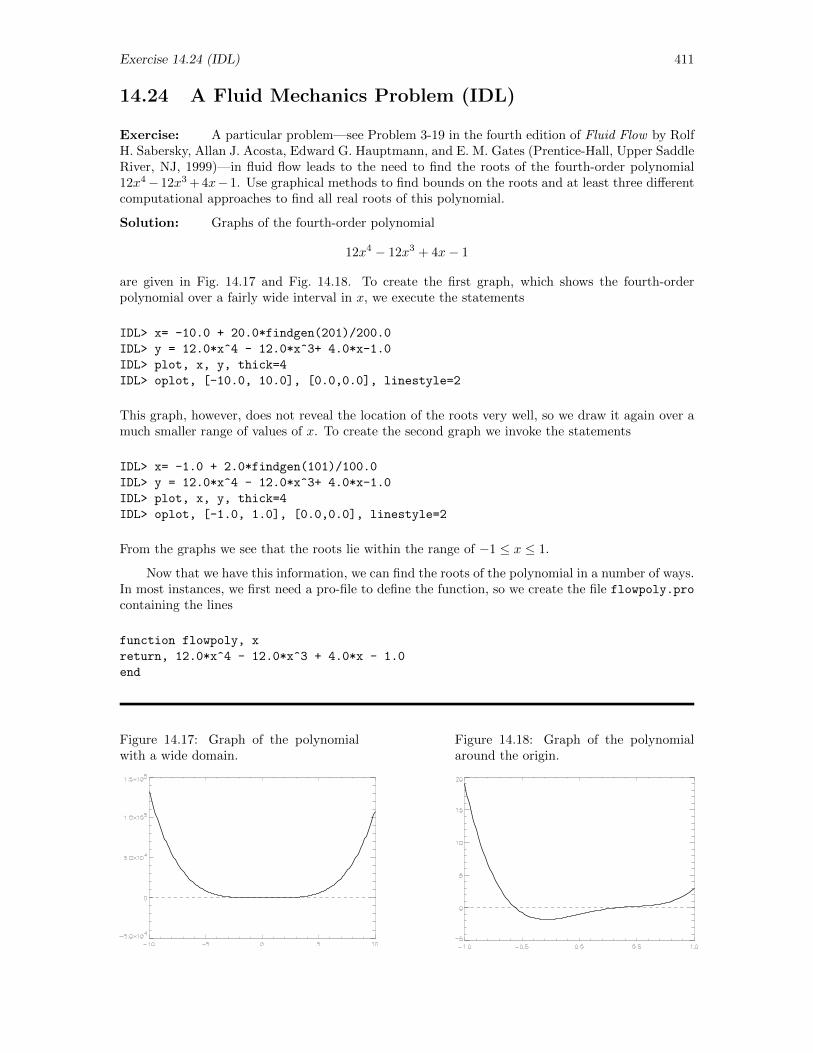
Exercise 14.24 (IDL) 411
14.24 A Fluid Mechanics Problem (IDL)
Exercise: A particular problem—see Problem 3-19 in the fourth edition of Fluid Flow by RolfH. Sabersky, Allan J. Acosta, Edward G. Hauptmann, and E. M. Gates (Prentice-Hall, Upper SaddleRiver, NJ, 1999)—in fluid flow leads to the need to find the roots of the fourth-order polynomial12x4−12x3 + 4x−1. Use graphical methods to find bounds on the roots and at least three differentcomputational approaches to find all real roots of this polynomial.
Solution: Graphs of the fourth-order polynomial
12x4 − 12x3 + 4x− 1
are given in Fig. 14.17 and Fig. 14.18. To create the first graph, which shows the fourth-orderpolynomial over a fairly wide interval in x, we execute the statements
IDL> x= -10.0 + 20.0*findgen(201)/200.0
IDL> y = 12.0*x^4 - 12.0*x^3+ 4.0*x-1.0
IDL> plot, x, y, thick=4
IDL> oplot, [-10.0, 10.0], [0.0,0.0], linestyle=2
This graph, however, does not reveal the location of the roots very well, so we draw it again over amuch smaller range of values of x. To create the second graph we invoke the statements
IDL> x= -1.0 + 2.0*findgen(101)/100.0
IDL> y = 12.0*x^4 - 12.0*x^3+ 4.0*x-1.0
IDL> plot, x, y, thick=4
IDL> oplot, [-1.0, 1.0], [0.0,0.0], linestyle=2
From the graphs we see that the roots lie within the range of −1 ≤ x ≤ 1.
Now that we have this information, we can find the roots of the polynomial in a number of ways.In most instances, we first need a pro-file to define the function, so we create the file flowpoly.pro
containing the lines
function flowpoly, x
return, 12.0*x^4 - 12.0*x^3 + 4.0*x - 1.0
end
Figure 14.17: Graph of the polynomialwith a wide domain.
Figure 14.18: Graph of the polynomialaround the origin.
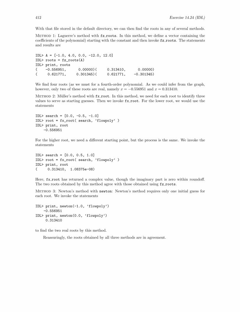
412 Exercise 14.24 (IDL)
With that file stored in the default directory, we can then find the roots in any of several methods.
Method 1: Laguerre’s method with fz roots. In this method, we define a vector containing thecoefficients of the polynomial) starting with the constant and then invoke fz roots. The statementsand results are
IDL> A = [-1.0, 4.0, 0.0, -12.0, 12.0]
IDL> roots = fz_roots(A)
IDL> print, roots
( -0.556951, 0.00000)( 0.313410, 0.00000)
( 0.621771, 0.301345)( 0.621771, -0.301345)
We find four roots (as we must for a fourth-order polynomial. As we could infer from the graph,however, only two of these roots are real, namely x = −0.556951 and x = 0.313410.
Method 2: Muller’s method with fx root. In this method, we need for each root to identify threevalues to serve as starting guesses. Then we invoke fx root. For the lower root, we would use thestatements
IDL> search = [0.0, -0.5, -1.0]
IDL> root = fx_root( search, ’flowpoly’ )
IDL> print, root
-0.556951
For the higher root, we need a different starting point, but the process is the same. We invoke thestatements
IDL> search = [0.0, 0.5, 1.0]
IDL> root = fx_root( search, ’flowpoly’ )
IDL> print, root
( 0.313410, 1.08375e-08)
Here, fx root has returned a complex value, though the imaginary part is zero within roundoff.The two roots obtained by this method agree with those obtained using fz roots.
Method 3: Newton’s method with newton: Newton’s method requires only one initial guess foreach root. We invoke the statements
IDL> print, newton(-1.0, ’flowpoly’)
-0.556951
IDL> print, newton(0.0, ’flowpoly’)
0.313410
to find the two real roots by this method.
Reassuringly, the roots obtained by all three methods are in agreement.
Exercise 14.18 (Mathematica) 413
14.18 Single-Slit Diffraction (Mathematica)
Exercise: The intensity I(x) in the diffraction pattern produced by a single slit is given by
I(x)
I0=
sin2 x
x2
where I0 is the intensity in the center and x is related to the position of the observation point awayfrom the central maximum. The zeroes in this pattern are easy to locate (they occur at x = nπ,n = 0,±1,±2, . . .). Careful location of the maxima, however, is more complicated. They don’t occurwhere sin2 x = 1 because of the influence of the denominator that steadily increases as x increases.Locate the positions of the first half dozen maxima in this pattern, which—basically—is a requestto find the roots of the derivative of the function (though note that not all roots correspond tomaxima). Use at least three different methods and at least two different computational tools, andcompare the results. Do your results confirm that the roots approach odd multiples of 1
2π as theybecome large? Optional : You might also find it interesting to approximate the function with a powerseries expansion for sinx, keeping quite a few terms but converting the root finding problem intothat of finding the roots of a polynomial. Then, use methods for finding roots of polynomials andsee if you can come to understand how accuracy depends on how many terms you keep and whichroot you seek.
Solution: The intensity I(x) in the diffraction pattern produced by a single slit is given by
I(x)
Io=
sin2 x
x2
A graph of this function can be made easily in Mathematica with the statements
In[1]:= i = Sin[x]^2/x^2;
In[2]:= g = Table[c, GrayLevel[1] , c, 20];
In[3]:= Plot[i, x, -5.0, 20.0, PlotStyle -> AbsoluteThickness[3],
AxesLabel -> "x", "i", GridLines -> g, None]
The resulting graph is shown in Fig. 14.19.
We want to find the maxima of the function. The maxima occur at every other root of (I/Io)′.
Thus we find the maxima by finding the roots of (I/Io)′ in the regions where the graph shows a
maxima. One way to find the roots is with the FindRoot function. To find the roots with thisfunction, we execute the statements5
In[4]:= d = D[i, x]
Out[4]=2 cos(x) sin(x)
x2− 2 sin[x]2
x3
In[5]:= FindRoot[d == 0, x, -0.5]
Out[5]=x→ 2.008289379149778× 10⁻¹¹
In[6]:= FindRoot[d == 0, x, 4.0]
Out[6]= x→ 4.49341
In[7]:= N[3*Pi/2] - %[[1, 2]]
Out[7]= 0.21898
5The FindRoot function is inconsistent and will not always return the closest root. For example, entering an initialcondition of x = 7.0 will not return 7.72524 as expected, but rather return 10.9041
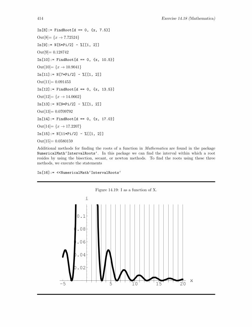
414 Exercise 14.18 (Mathematica)
In[8]:= FindRoot[d == 0, x, 7.5]
Out[8]= x→ 7.72524
In[9]:= N[5*Pi/2] - %[[1, 2]]
Out[9]= 0.128742
In[10]:= FindRoot[d == 0, x, 10.5]
Out[10]= x→ 10.9041
In[11]:= N[7*Pi/2] - %[[1, 2]]
Out[11]= 0.091453
In[12]:= FindRoot[d == 0, x, 13.5]
Out[12]= x→ 14.0662
In[13]:= N[9*Pi/2] - %[[1, 2]]
Out[13]= 0.0709792
In[14]:= FindRoot[d == 0, x, 17.0]
Out[14]= x→ 17.2207
In[15]:= N[11*Pi/2] - %[[1, 2]]
Out[15]= 0.0580159
Additional methods for finding the roots of a function in Mathematica are found in the packageNumericalMath‘IntervalRoots‘. In this package we can find the interval within which a rootresides by using the bisection, secant, or newton methods. To find the roots using these threemethods, we execute the statements
In[16]:= <<NumericalMath‘IntervalRoots‘
Figure 14.19: I as a function of X.
-5 5 10 15 20x
0.02
0.04
0.06
0.08
0.1
i
Exercise 14.18 (Mathematica) 415
In[17]:= IntervalBisection[d, x, Interval[4.0, 5.0], 0.0001,
MaxRecursion -> 20]
Out[17]= Interval[4.49335, 4.49347]
In[18]:= IntervalBisection[d, x, Interval[7.0, 8.0], 0.0001,
MaxRecursion -> 20]
Out[18]= Interval[7.72522, 7.72528]
In[19]:= IntervalSecant[d, x, Interval[4.0, 5.0], 0.0001,
MaxRecursion -> 20]
Out[19]= Interval[4.49341, 4.49341]
In[20]:= IntervalSecant[d, x, Interval[7.0, 8.0], 0.0001,
MaxRecursion -> 20]
Out[20]= Interval[7.72524, 7.72526]
In[21]:= IntervalNewton[d, x, Interval[4.0, 5.0], 0.0001,
MaxRecursion -> 20]
Out[21]= Interval[4.49336, 4.49345]
In[22]:= IntervalNewton[d, x, Interval[7.0, 8.0], 0.0001,
MaxRecursion -> 20]
Out[22]= Interval[7.72525, 7.72525]
From these methods, we see that secant and newton methods converge on the root faster thanthe bisection method, but they all converge to the same root. By looking at the roots and thecomparisons that followed, we see that the maxima are found at x ≈ 0, 3π/2, 5π/2, 7π/2, etc.Furthermore, we see that the difference between the root and the multiple of π/2 lessens as the sizeof the root increases. So, the maxima do indeeed approach odd multiples of π/2 as the roots becomelarge.
If we approximate the function with a power series, we find we are limited in our ability tofind the desired roots. First, we find that the number of the polynomial’s real roots increases asthe number of terms in the polynomial increases. In the data presented here, we see only three realroots. If the number of terms is increased to 40, the number of real roots increases to 11. The otherroots to the polynomial are imaginary. Furthermore, we see that as the number of terms increases,the accuracy of the roots increases. To explore this power series approximation, we execute thestatements
In[23]:= iserone = Series[i, x, 0, 4];
In[24]:= Normal[%]
Out[24]= 1− x2
3+
2x4
45
In[25]:= dserone = D[%, x]
Out[25]=−2x
3+
8x3
45
In[26]:= NSolve[dserone == 0, x]
Out[26]= x→ −1.93649, x→ 0., x→ 1.93649
In[27]:= isertwo = Series[i, x, 0, 8];
In[27]:= Normal[%];
In[29]:= dsertwo = D[%, x];
416 Exercise 14.18 (Mathematica)
In[30]:= NSolve[dsertwo == 0, x]
Out[30]= x→ −2.70384− 1.47083i, x→ −2.70384 + 1.47083i, x→ −2.56519,x→ 0., x→ 2.56519, x→ 2.70384− 1.47083i,x→ 2.70384 + 1.47083i
In[31]:= iser = Series[i, x, 0, 20];
In[32]:= Normal[%];
In[33]:= dser = D[%, x];
In[34]:= NSolve[dser == 0, x]
Out[34]= x→ −5.1619− 3.37102i, x→ −5.1619 + 3.37102i, x→ −5.05779− 1.60258i,x→ −5.05779 + 1.60258i, x→ −4.81827− 5.97602i, x→ −4.81827 + 5.97602i,x→ −4.61423− 0.219485i, x→ −4.61423 + 0.219485i,x→ −3.14155, x→ 0., x→ 3.14155,x→ 4.61423− 0.219485i, x→ 4.61423 + 0.219485i, x→ 4.81827− 5.97602i,x→ 4.81827 + 5.97602i, x→ 5.05779− 1.60258i, x→ 5.05779 + 1.60258i,x→ 5.1619− 3.37102i, x→ 5.1619 + 3.37102i
In[35]:= FindRoot[dser == 0, x, -0.5]
Out[35]= (x→ 8.854689822080514× 10⁻¹²)
In[36]:= FindRoot[dser == 0, x, -0.5]
Out[36]= x→ 3.14155
In[37]:= FindRoot[dser == 0, x, -0.5]
Out[37]= x→ 7.28211
In[38]:= IntervalBisection[dser, x, Interval[7.0, 8.0], 0.0001,
MaxRecursion -> 20]
Out[38]= Interval[]
We enter similar statements to explore this topic further.
Exercise 14.19 (Mathematica) 417
14.19 Roots of J0(x) (Mathematica)
Exercise: Using at least three different methods and at least two different computationaltools, find the first half dozen roots of the zeroth-order Bessel function J0(x). Note that theseroots are related to the radii of circular nodes in some of the vibrations of a circular membrane.The values of these roots tabulated in Abramowitz and Stegun6 are 2.4048255577, 5.5200781103,8.6537279129, 11.7915344391, 14.9309177086, 18.0710639679. Hint : Most computational tools havebuilt-in capabilities for evaluating the Bessel functions. Consult the appropriate vendor manuals.
Solution: We wish to know the first half dozen roots of the zeroth-order Bessel function.The values of the roots as tabulated by Abramowitz and Stegun are 2.40485 55577, 5.52007 81103,8.65372 79129, 11.79153 44391, 14.93091 77086, and 18.07106 39679.
The Bessel function we desire can be found in Mathematica under the name BesselJ[0, x]. To useFindRoot function, we need only call up the Bessel function and give Mathematica a starting point.So, we find the roots by executing the statements
In[1]:= BesselJ[0, x];
In[2]:= FindRoot[%1 == 0, x, 2.0]
Out[2] = x→ 2.40483
In[3]:= FindRoot[%1 == 0, x, 5.0]
Out[3] = x→ 5.52008
In[4]:= FindRoot[%1 == 0, x, 8.0]
Out[4] = x→ 8.65373
In[5]:= FindRoot[%1 == 0, x, 11.0]
Out[5] = x→ 11.7915
We can continue this way until the first half dozen roots have been found. By knowing ahead oftime what the roots are, it is very easy to give good useful starting points to Mathematica. If wedid not know the roots already we could create a graph to find the general area of the roots. Wecreate a graph by executing the statements
In[6]:= g = Table[c, GrayLevel[1] , c, 20];
In[7]:= Plot[%1, x, 0.0, 20.0, PlotStyle -> AbsoluteThickness[3],
AxesLabel -> "x", "BesselJ", GridLines -> g, None]
From this graph (seen in Fig. 14.20) we can obtain useful starting points for use in the FindRoot
function. However, Mathematica provides a much quicker way to find the roots of the zeroth-orderBessel function. If we load the package NumericalMath‘BesselZeros‘, we can make use of theBesselJZeros function. This function takes as its arguments the order of the Bessel function andthe number of roots desired and then returns those roots. So, we can also find the first half dozenroots by executing the statements
In[8]:= << NumericalMath‘BesselZeros‘
In[1]:= BesselJZeros[0, 6]
Out[2] = 2.40483, 5.52008, 8.65373, 11.7915, 14.9309, 18.0711
6M. Abramowitz and I. A. Stegun, Handbook of Mathematical Functions, U. S. Department of Commerce, AppliedMathematics Series #55, 1964.
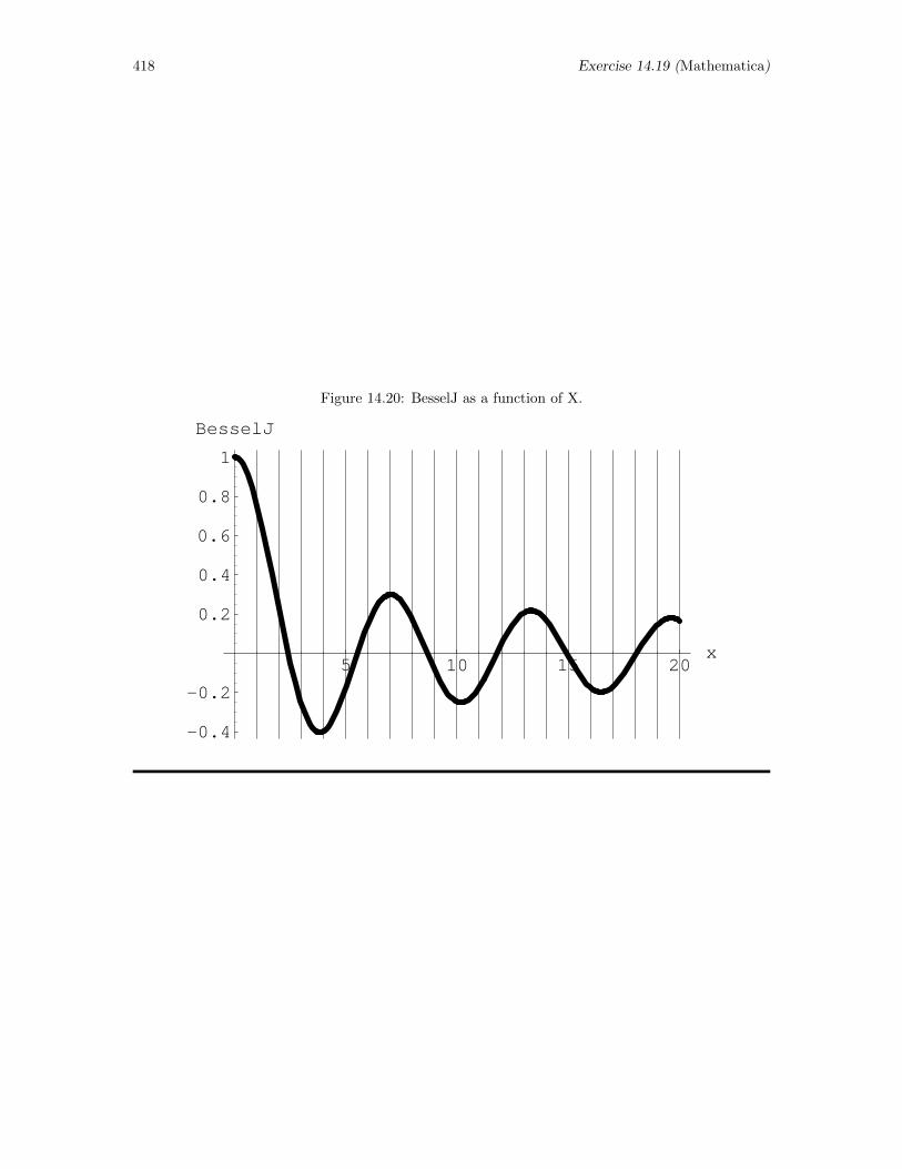
418 Exercise 14.19 (Mathematica)
Figure 14.20: BesselJ as a function of X.
5 10 15 20x
-0.4
-0.2
0.2
0.4
0.6
0.8
1
BesselJ
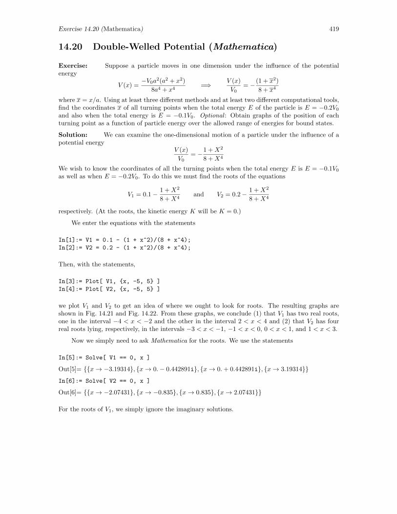
Exercise 14.20 (Mathematica) 419
14.20 Double-Welled Potential (Mathematica)
Exercise: Suppose a particle moves in one dimension under the influence of the potentialenergy
V (x) =−V0a
2(a2 + x2)
8a4 + x4=⇒ V (x)
V0= − (1 + x2)
8 + x4
where x = x/a. Using at least three different methods and at least two different computational tools,find the coordinates x of all turning points when the total energy E of the particle is E = −0.2V0
and also when the total energy is E = −0.1V0. Optional : Obtain graphs of the position of eachturning point as a function of particle energy over the allowed range of energies for bound states.
Solution: We can examine the one-dimensional motion of a particle under the influence of apotential energy
V (x)
V0= −1 +X2
8 +X4
We wish to know the coordinates of all the turning points when the total energy E is E = −0.1V0
as well as when E = −0.2V0. To do this we must find the roots of the equations
V1 = 0.1− 1 +X2
8 +X4and V2 = 0.2− 1 +X2
8 +X4
respectively. (At the roots, the kinetic energy K will be K = 0.)
We enter the equations with the statements
In[1]:= V1 = 0.1 - (1 + x^2)/(8 + x^4);
In[2]:= V2 = 0.2 - (1 + x^2)/(8 + x^4);
Then, with the statements,
In[3]:= Plot[ V1, x, -5, 5 ]
In[4]:= Plot[ V2, x, -5, 5 ]
we plot V1 and V2 to get an idea of where we ought to look for roots. The resulting graphs areshown in Fig. 14.21 and Fig. 14.22. From these graphs, we conclude (1) that V1 has two real roots,one in the interval −4 < x < −2 and the other in the interval 2 < x < 4 and (2) that V2 has fourreal roots lying, respectively, in the intervals −3 < x < −1, −1 < x < 0, 0 < x < 1, and 1 < x < 3.
Now we simply need to ask Mathematica for the roots. We use the statements
In[5]:= Solve[ V1 == 0, x ]
Out[5]= x→ −3.19314, x→ 0.− 0.442891i, x→ 0.+ 0.442891i, x→ 3.19314
In[6]:= Solve[ V2 == 0, x ]
Out[6]= x→ −2.07431, x→ −0.835, x→ 0.835, x→ 2.07431
For the roots of V1, we simply ignore the imaginary solutions.
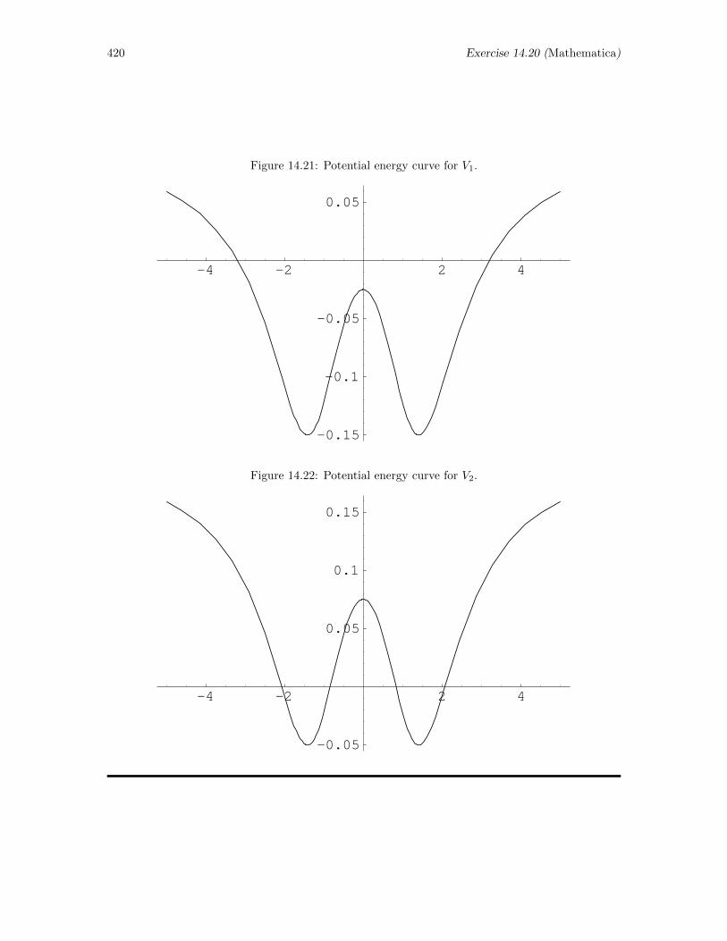
420 Exercise 14.20 (Mathematica)
Figure 14.21: Potential energy curve for V1.
-4 -2 2 4
-0.15
-0.1
-0.05
0.05
Figure 14.22: Potential energy curve for V2.
-4 -2 2 4
-0.05
0.05
0.1
0.15
Exercise 14.12 (FORTRAN) 421
14.12 Square Root by Newton’s Method (FORTRAN)
Exercise: One way to find the square root of a (positive) number a is to find the root of thefunction f(x) = x2−a. (a) Apply Newton’s method symbolically to show that xn+1 = (xn+a/xn)/2.(b) Using a pocket calculator and starting with the guess x0 = 2, work out the first few iteratesby hand and note how quickly this algorithm converges to
√2 = 1.41421. (This algorithm is the
algorithm that most pocket calculators invoke when the square root key is pressed.) (c) Usingwhatever computational tool appeals to you, write a program that asks for the value of a, an initialguess for
√a, and a tolerance and then implements Newton’s method to find
√a, printing out each
iterate along the way and stopping automatically when successive iterates differ by less than thespecified tolerance.
Solution: (a) The square root of a number a can be found by locating the roots of the equationf(x) = x2 − a. With the shorthand notation fn = f(xn) and f ′n = df(x)/dx|xn , we can writeNewton’s method for the function of interest in the form
xn+1 = xn −fnf ′n
= xn −x2n − a2xn
= xn −xn2
+a
2xn=
1
2
(xn +
a
xn
)
(b) With a pocket calculator, if we start with a = 2 and the initial guess x0 = 2, we then find that
x1 =1
2
(x0 +
2
x0
)=
1
2
(2 +
2
2
)= 0.5× 3 = 1.5
Then, the next iteration gives
x2 =1
2
(x1 +
2
x1
)=
1
2
(1.5 +
2
1.5
)= 1.4166667
and the next iteration gives
x3 =1
2
(x2 +
2
x2
)=
1
2
(1.4166667 +
2
1.416667
)= 1.4142157
and the next gives
x4 =1
2
(x3 +
2
x3
)=
1
2
(1.4142157 +
2
1.4142157
)= 1.4142136
The square root of 2 obtained with the square root key on this pocket calculator gives 1.4142136, sofour iterations have apparently given us the square root of 2 to seven digits after the decimal place.
(c) Using basic commands, it is not difficult to construct a program that utilizes Newton’s methodto find the square root of a number. A sample FORTRAN program is shown at the top of the nextpage. The statement diff = toler + 1.0 is included before the loop to make sure that diff isindeed greater than toler when the loop is started. Note also that the tolerance is an absolutetolerance, and that each iterate is printed so the user can see how quickly the algorithm converges.
Once this program has been stored in the default directory with the name squareroot.f, wewould compile and run the program to find the square root of 2 with the statements
f77 -o squareroot.xf squareroot.f
./squareroot.xf
Number whose root is to be found: 2.0
Initial guess: 1.0
Absolute tolerance: 0.0001
Iterative results:
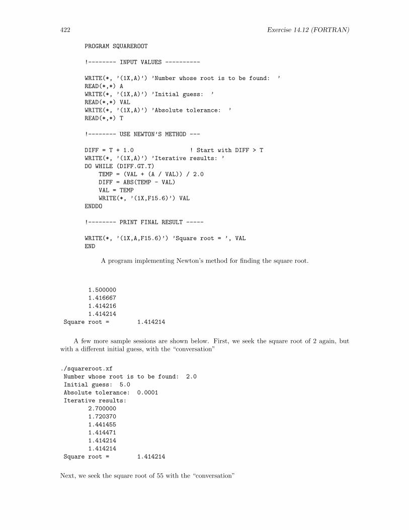
422 Exercise 14.12 (FORTRAN)
PROGRAM SQUAREROOT
!-------- INPUT VALUES ----------
WRITE(*, ’(1X,A)’) ’Number whose root is to be found: ’
READ(*,*) A
WRITE(*, ’(1X,A)’) ’Initial guess: ’
READ(*,*) VAL
WRITE(*, ’(1X,A)’) ’Absolute tolerance: ’
READ(*,*) T
!-------- USE NEWTON’S METHOD ---
DIFF = T + 1.0 ! Start with DIFF > T
WRITE(*, ’(1X,A)’) ’Iterative results: ’
DO WHILE (DIFF.GT.T)
TEMP = (VAL + (A / VAL)) / 2.0
DIFF = ABS(TEMP - VAL)
VAL = TEMP
WRITE(*, ’(1X,F15.6)’) VAL
ENDDO
!-------- PRINT FINAL RESULT -----
WRITE(*, ’(1X,A,F15.6)’) ’Square root = ’, VAL
END
A program implementing Newton’s method for finding the square root.
1.500000
1.416667
1.414216
1.414214
Square root = 1.414214
A few more sample sessions are shown below. First, we seek the square root of 2 again, butwith a different initial guess, with the “conversation”
./squareroot.xf
Number whose root is to be found: 2.0
Initial guess: 5.0
Absolute tolerance: 0.0001
Iterative results:
2.700000
1.720370
1.441455
1.414471
1.414214
1.414214
Square root = 1.414214
Next, we seek the square root of 55 with the “conversation”

Exercise 14.12 (FORTRAN) 423
./squareroot.xf
Number whose root is to be found: 55.0
Initial guess: 7.0
Absolute tolerance: 0.0001
Iterative results:
7.428572
7.416209
7.416199
Square root = 7.416199
In all these examples, convergence to five digits after the decimal point occurs in no more than halfa dozen iterations.
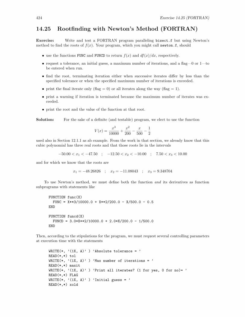
424 Exercise 14.25 (FORTRAN)
14.25 Rootfinding with Newton’s Method (FORTRAN)
Exercise: Write and test a FORTRAN program paralleling bisect.f but using Newton’smethod to find the roots of f(x). Your program, which you might call newton.f, should
• use the functions FUNC and FUNCD to return f(x) and df(x)/dx, respectively.
• request a tolerance, an initial guess, a maximum number of iterations, and a flag—0 or 1—tobe entered when run.
• find the root, terminating iteration either when successive iterates differ by less than thespecified tolerance or when the specified maximum number of iterations is exceeded.
• print the final iterate only (flag = 0) or all iterates along the way (flag = 1).
• print a warning if iteration is terminated because the maximum number of iterates was ex-ceeded.
• print the root and the value of the function at that root.
Solution: For the sake of a definite (and testable) program, we elect to use the function
V (x) =x3
10000+
x2
200− x
500− 1
2
used also in Section 12.1.1 as ab example. From the work in that section, we already know that thiscubic polynomial has three real roots and that those roots lie in the intervals
−50.00 < x1 < −47.50 ; −12.50 < x2 < −10.00 ; 7.50 < x3 < 10.00
and for which we know that the roots are
x1 = −48.26826 ; x2 = −11.08043 ; x3 = 9.348704
To use Newton’s method, we must define both the function and its derivatives as functionsubprograms with statements like
FUNCTION func(X)
FUNC = X**3/10000.0 + X**2/200.0 - X/500.0 - 0.5
END
FUNCTION funcd(X)
FUNCD = 3.0*X**2/10000.0 + 2.0*X/200.0 - 1/500.0
END
Then, according to the stipulations for the program, we must request several controlling parametersat execution time with the statements
WRITE(*, ’(1X, A)’ ) ’Absolute tolerance = ’
READ(*,*) tol
WRITE(*, ’(1X, A)’ ) ’Max number of iterations = ’
READ(*,*) maxit
WRITE(*, ’(1X, A)’ ) ’Print all iterates? (1 for yes, 0 for no)= ’
READ(*,*) FLAG
WRITE(*, ’(1X, A)’ ) ’Initial guess = ’
READ(*,*) xold
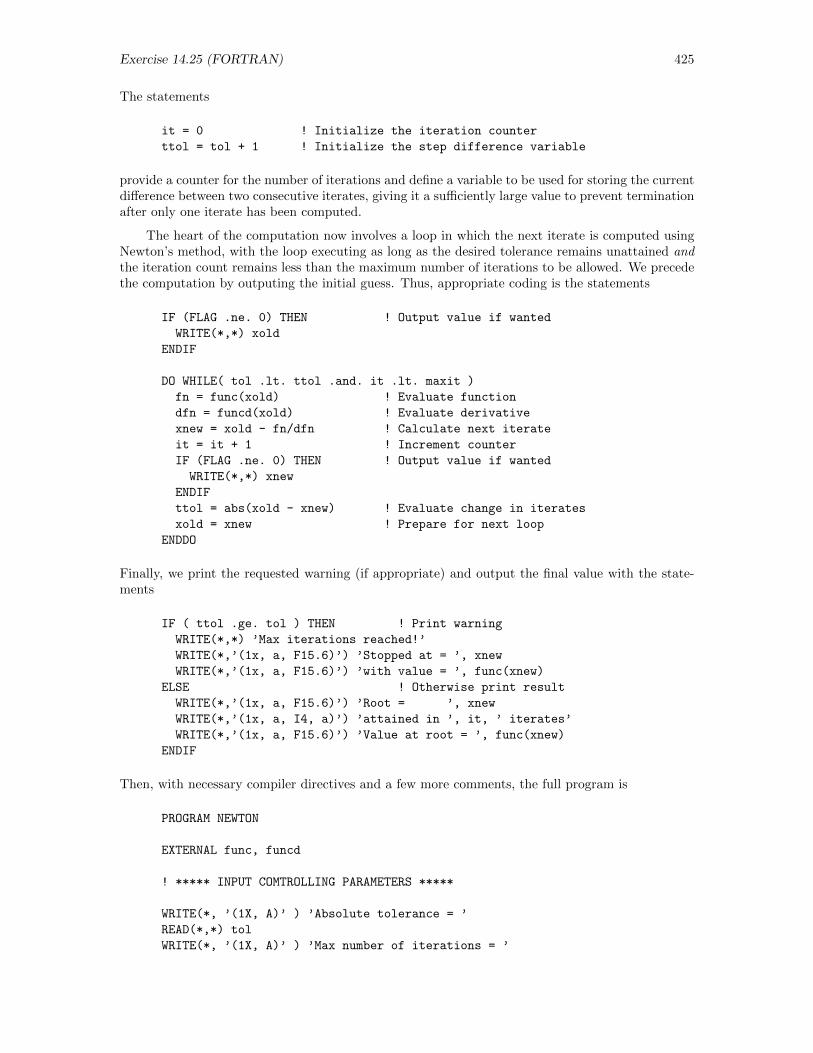
Exercise 14.25 (FORTRAN) 425
The statements
it = 0 ! Initialize the iteration counter
ttol = tol + 1 ! Initialize the step difference variable
provide a counter for the number of iterations and define a variable to be used for storing the currentdifference between two consecutive iterates, giving it a sufficiently large value to prevent terminationafter only one iterate has been computed.
The heart of the computation now involves a loop in which the next iterate is computed usingNewton’s method, with the loop executing as long as the desired tolerance remains unattained andthe iteration count remains less than the maximum number of iterations to be allowed. We precedethe computation by outputing the initial guess. Thus, appropriate coding is the statements
IF (FLAG .ne. 0) THEN ! Output value if wanted
WRITE(*,*) xold
ENDIF
DO WHILE( tol .lt. ttol .and. it .lt. maxit )
fn = func(xold) ! Evaluate function
dfn = funcd(xold) ! Evaluate derivative
xnew = xold - fn/dfn ! Calculate next iterate
it = it + 1 ! Increment counter
IF (FLAG .ne. 0) THEN ! Output value if wanted
WRITE(*,*) xnew
ENDIF
ttol = abs(xold - xnew) ! Evaluate change in iterates
xold = xnew ! Prepare for next loop
ENDDO
Finally, we print the requested warning (if appropriate) and output the final value with the state-ments
IF ( ttol .ge. tol ) THEN ! Print warning
WRITE(*,*) ’Max iterations reached!’
WRITE(*,’(1x, a, F15.6)’) ’Stopped at = ’, xnew
WRITE(*,’(1x, a, F15.6)’) ’with value = ’, func(xnew)
ELSE ! Otherwise print result
WRITE(*,’(1x, a, F15.6)’) ’Root = ’, xnew
WRITE(*,’(1x, a, I4, a)’) ’attained in ’, it, ’ iterates’
WRITE(*,’(1x, a, F15.6)’) ’Value at root = ’, func(xnew)
ENDIF
Then, with necessary compiler directives and a few more comments, the full program is
PROGRAM NEWTON
EXTERNAL func, funcd
! ***** INPUT COMTROLLING PARAMETERS *****
WRITE(*, ’(1X, A)’ ) ’Absolute tolerance = ’
READ(*,*) tol
WRITE(*, ’(1X, A)’ ) ’Max number of iterations = ’
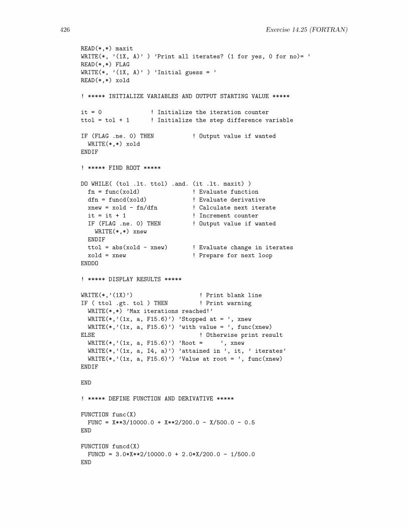
426 Exercise 14.25 (FORTRAN)
READ(*,*) maxit
WRITE(*, ’(1X, A)’ ) ’Print all iterates? (1 for yes, 0 for no)= ’
READ(*,*) FLAG
WRITE(*, ’(1X, A)’ ) ’Initial guess = ’
READ(*,*) xold
! ***** INITIALIZE VARIABLES AND OUTPUT STARTING VALUE *****
it = 0 ! Initialize the iteration counter
ttol = tol + 1 ! Initialize the step difference variable
IF (FLAG .ne. 0) THEN ! Output value if wanted
WRITE(*,*) xold
ENDIF
! ***** FIND ROOT *****
DO WHILE( (tol .lt. ttol) .and. (it .lt. maxit) )
fn = func(xold) ! Evaluate function
dfn = funcd(xold) ! Evaluate derivative
xnew = xold - fn/dfn ! Calculate next iterate
it = it + 1 ! Increment counter
IF (FLAG .ne. 0) THEN ! Output value if wanted
WRITE(*,*) xnew
ENDIF
ttol = abs(xold - xnew) ! Evaluate change in iterates
xold = xnew ! Prepare for next loop
ENDDO
! ***** DISPLAY RESULTS *****
WRITE(*,’(1X)’) ! Print blank line
IF ( ttol .gt. tol ) THEN ! Print warning
WRITE(*,*) ’Max iterations reached!’
WRITE(*,’(1x, a, F15.6)’) ’Stopped at = ’, xnew
WRITE(*,’(1x, a, F15.6)’) ’with value = ’, func(xnew)
ELSE ! Otherwise print result
WRITE(*,’(1x, a, F15.6)’) ’Root = ’, xnew
WRITE(*,’(1x, a, I4, a)’) ’attained in ’, it, ’ iterates’
WRITE(*,’(1x, a, F15.6)’) ’Value at root = ’, func(xnew)
ENDIF
END
! ***** DEFINE FUNCTION AND DERIVATIVE *****
FUNCTION func(X)
FUNC = X**3/10000.0 + X**2/200.0 - X/500.0 - 0.5
END
FUNCTION funcd(X)
FUNCD = 3.0*X**2/10000.0 + 2.0*X/200.0 - 1/500.0
END
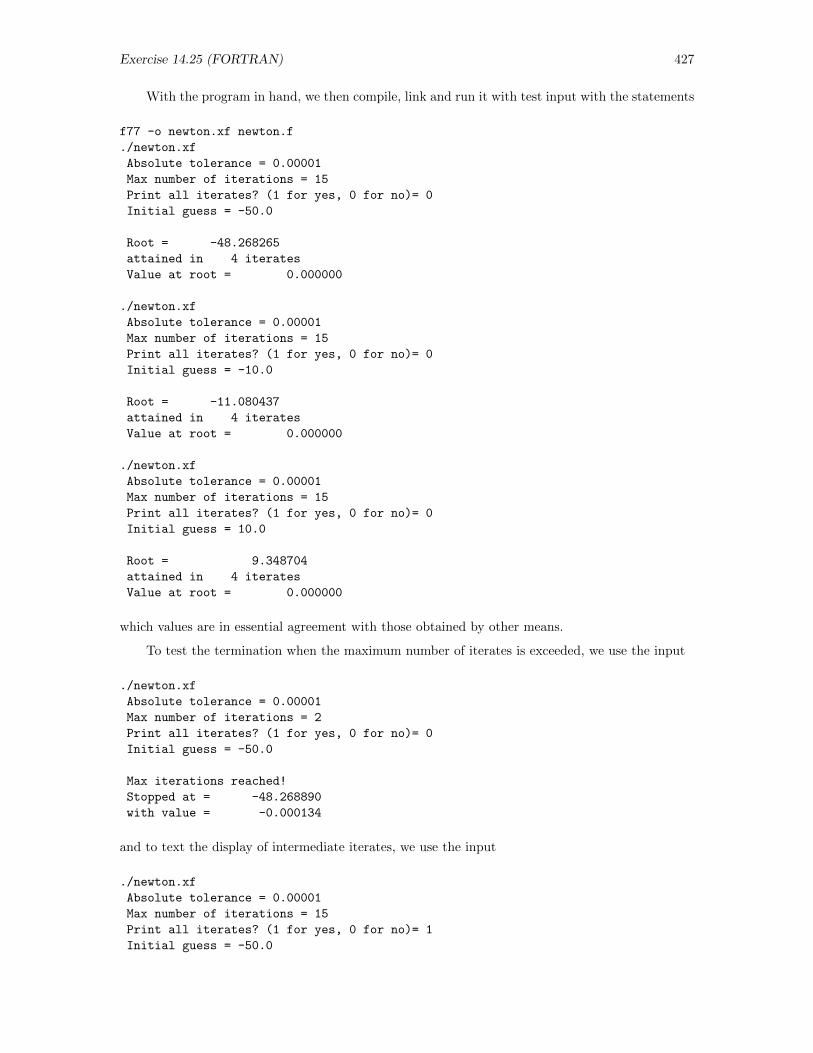
Exercise 14.25 (FORTRAN) 427
With the program in hand, we then compile, link and run it with test input with the statements
f77 -o newton.xf newton.f
./newton.xf
Absolute tolerance = 0.00001
Max number of iterations = 15
Print all iterates? (1 for yes, 0 for no)= 0
Initial guess = -50.0
Root = -48.268265
attained in 4 iterates
Value at root = 0.000000
./newton.xf
Absolute tolerance = 0.00001
Max number of iterations = 15
Print all iterates? (1 for yes, 0 for no)= 0
Initial guess = -10.0
Root = -11.080437
attained in 4 iterates
Value at root = 0.000000
./newton.xf
Absolute tolerance = 0.00001
Max number of iterations = 15
Print all iterates? (1 for yes, 0 for no)= 0
Initial guess = 10.0
Root = 9.348704
attained in 4 iterates
Value at root = 0.000000
which values are in essential agreement with those obtained by other means.
To test the termination when the maximum number of iterates is exceeded, we use the input
./newton.xf
Absolute tolerance = 0.00001
Max number of iterations = 2
Print all iterates? (1 for yes, 0 for no)= 0
Initial guess = -50.0
Max iterations reached!
Stopped at = -48.268890
with value = -0.000134
and to text the display of intermediate iterates, we use the input
./newton.xf
Absolute tolerance = 0.00001
Max number of iterations = 15
Print all iterates? (1 for yes, 0 for no)= 1
Initial guess = -50.0

428 Exercise 14.25 (FORTRAN)
-50.00000
-48.38710
-48.26889
-48.26826
-48.26826
Root = -48.268265
attained in 4 iterates
Value at root = 0.000000
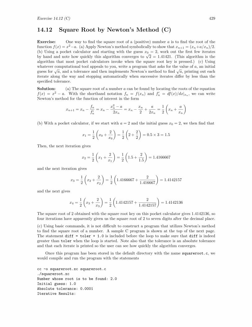
Exercise 14.12 (C) 429
14.12 Square Root by Newton’s Method (C)
Exercise: One way to find the square root of a (positive) number a is to find the root of thefunction f(x) = x2−a. (a) Apply Newton’s method symbolically to show that xn+1 = (xn+a/xn)/2.(b) Using a pocket calculator and starting with the guess x0 = 2, work out the first few iteratesby hand and note how quickly this algorithm converges to
√2 = 1.41421. (This algorithm is the
algorithm that most pocket calculators invoke when the square root key is pressed.) (c) Usingwhatever computational tool appeals to you, write a program that asks for the value of a, an initialguess for
√a, and a tolerance and then implements Newton’s method to find
√a, printing out each
iterate along the way and stopping automatically when successive iterates differ by less than thespecified tolerance.
Solution: (a) The square root of a number a can be found by locating the roots of the equationf(x) = x2 − a. With the shorthand notation fn = f(xn) and f ′n = df(x)/dx|xn , we can writeNewton’s method for the function of interest in the form
xn+1 = xn −fnf ′n
= xn −x2n − a2xn
= xn −xn2
+a
2xn=
1
2
(xn +
a
xn
)
(b) With a pocket calculator, if we start with a = 2 and the initial guess x0 = 2, we then find that
x1 =1
2
(x0 +
2
x0
)=
1
2
(2 +
2
2
)= 0.5× 3 = 1.5
Then, the next iteration gives
x2 =1
2
(x1 +
2
x1
)=
1
2
(1.5 +
2
1.5
)= 1.4166667
and the next iteration gives
x3 =1
2
(x2 +
2
x2
)=
1
2
(1.4166667 +
2
1.416667
)= 1.4142157
and the next gives
x4 =1
2
(x3 +
2
x3
)=
1
2
(1.4142157 +
2
1.4142157
)= 1.4142136
The square root of 2 obtained with the square root key on this pocket calculator gives 1.4142136, sofour iterations have apparently given us the square root of 2 to seven digits after the decimal place.
(c) Using basic commands, it is not difficult to construct a program that utilizes Newton’s methodto find the square root of a number. A sample C program is shown at the top of the next page.The statement diff = toler + 1.0 is included before the loop to make sure that diff is indeedgreater than toler when the loop is started. Note also that the tolerance is an absolute toleranceand that each iterate is printed so the user can see how quickly the algorithm converges.
Once this program has been stored in the default directory with the name squareroot.c, wewould compile and run the program with the statements
cc -o squareroot.xc squareroot.c
./squareroot.xc
Number whose root is to be found: 2.0
Initial guess: 1.0
Absolute tolerance: 0.0001
Iterative Results:
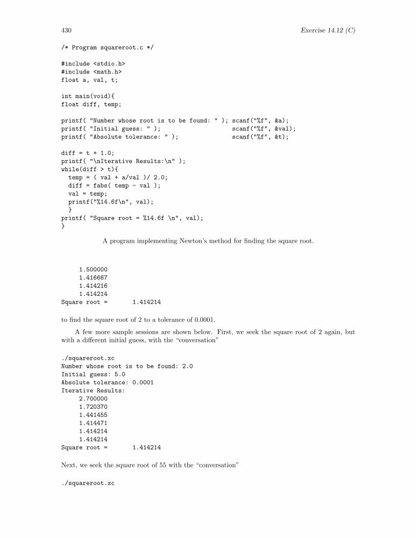
430 Exercise 14.12 (C)
/* Program squareroot.c */
#include <stdio.h>
#include <math.h>
float a, val, t;
int main(void)
float diff, temp;
printf( "Number whose root is to be found: " ); scanf("%f", &a);
printf( "Initial guess: " ); scanf("%f", &val);
printf( "Absolute tolerance: " ); scanf("%f", &t);
diff = t + 1.0;
printf( "\nIterative Results:\n" );
while(diff > t)
temp = ( val + a/val )/ 2.0;
diff = fabs( temp - val );
val = temp;
printf("%14.6f\n", val);
printf( "Square root = %14.6f \n", val);
A program implementing Newton’s method for finding the square root.
1.500000
1.416667
1.414216
1.414214
Square root = 1.414214
to find the square root of 2 to a tolerance of 0.0001.
A few more sample sessions are shown below. First, we seek the square root of 2 again, butwith a different initial guess, with the “conversation”
./squareroot.xc
Number whose root is to be found: 2.0
Initial guess: 5.0
Absolute tolerance: 0.0001
Iterative Results:
2.700000
1.720370
1.441455
1.414471
1.414214
1.414214
Square root = 1.414214
Next, we seek the square root of 55 with the “conversation”
./squareroot.xc

Exercise 14.12 (C) 431
Number whose root is to be found: 55.0
Initial guess: 7.0
Absolute tolerance: 0.0001
Iterative Results:
7.428572
7.416209
7.416199
Square root = 7.416199
In all these examples, convergence to five digits after the decimal point occurs in no more than halfa dozen iterations.
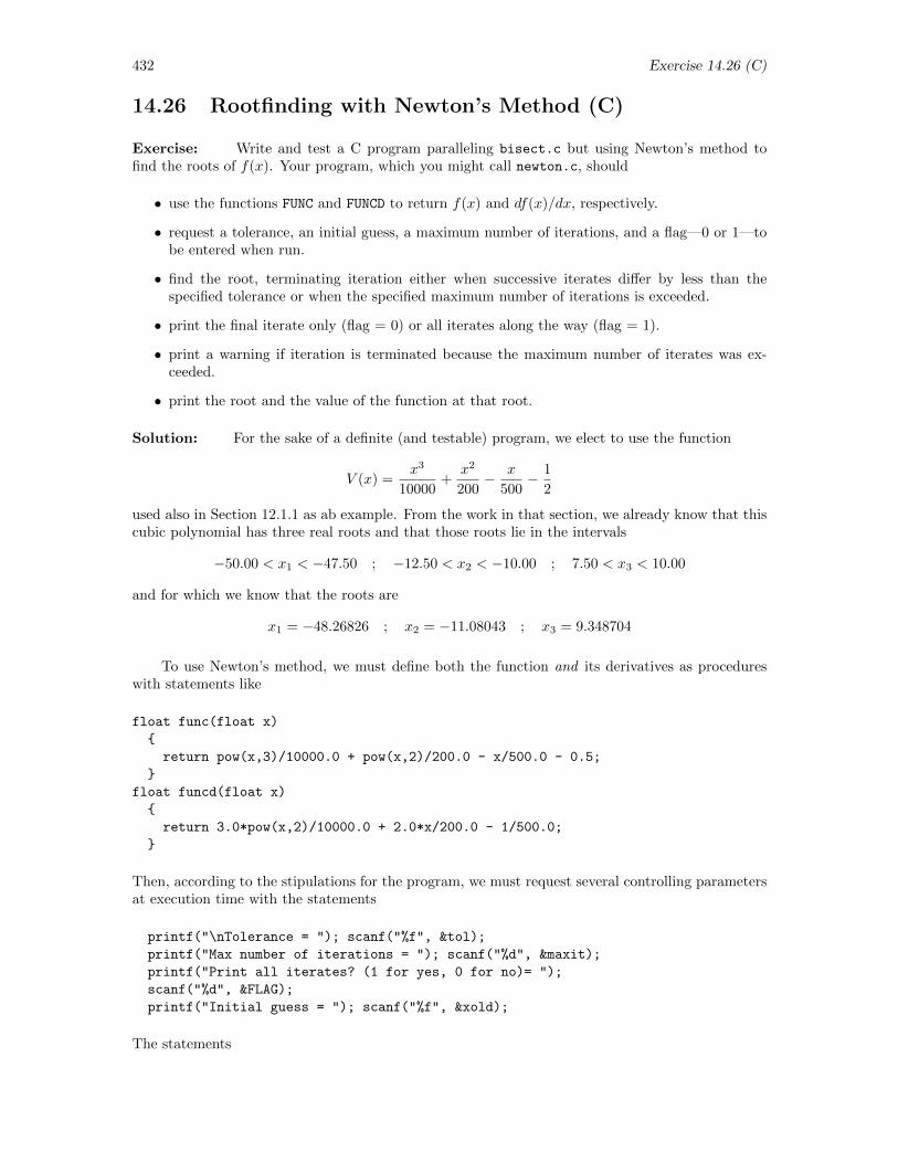
432 Exercise 14.26 (C)
14.26 Rootfinding with Newton’s Method (C)
Exercise: Write and test a C program paralleling bisect.c but using Newton’s method tofind the roots of f(x). Your program, which you might call newton.c, should
• use the functions FUNC and FUNCD to return f(x) and df(x)/dx, respectively.
• request a tolerance, an initial guess, a maximum number of iterations, and a flag—0 or 1—tobe entered when run.
• find the root, terminating iteration either when successive iterates differ by less than thespecified tolerance or when the specified maximum number of iterations is exceeded.
• print the final iterate only (flag = 0) or all iterates along the way (flag = 1).
• print a warning if iteration is terminated because the maximum number of iterates was ex-ceeded.
• print the root and the value of the function at that root.
Solution: For the sake of a definite (and testable) program, we elect to use the function
V (x) =x3
10000+
x2
200− x
500− 1
2
used also in Section 12.1.1 as ab example. From the work in that section, we already know that thiscubic polynomial has three real roots and that those roots lie in the intervals
−50.00 < x1 < −47.50 ; −12.50 < x2 < −10.00 ; 7.50 < x3 < 10.00
and for which we know that the roots are
x1 = −48.26826 ; x2 = −11.08043 ; x3 = 9.348704
To use Newton’s method, we must define both the function and its derivatives as procedureswith statements like
float func(float x)
return pow(x,3)/10000.0 + pow(x,2)/200.0 - x/500.0 - 0.5;
float funcd(float x)
return 3.0*pow(x,2)/10000.0 + 2.0*x/200.0 - 1/500.0;
Then, according to the stipulations for the program, we must request several controlling parametersat execution time with the statements
printf("\nTolerance = "); scanf("%f", &tol);
printf("Max number of iterations = "); scanf("%d", &maxit);
printf("Print all iterates? (1 for yes, 0 for no)= ");
scanf("%d", &FLAG);
printf("Initial guess = "); scanf("%f", &xold);
The statements
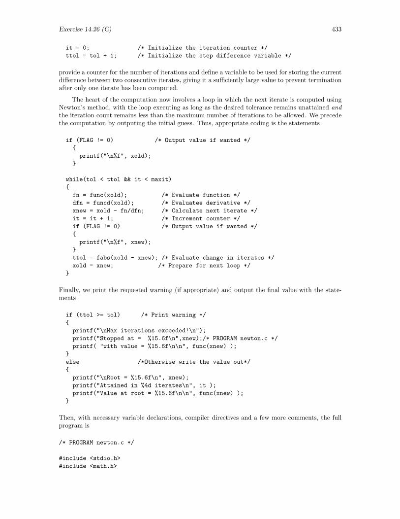
Exercise 14.26 (C) 433
it = 0; /* Initialize the iteration counter */
ttol = tol + 1; /* Initialize the step difference variable */
provide a counter for the number of iterations and define a variable to be used for storing the currentdifference between two consecutive iterates, giving it a sufficiently large value to prevent terminationafter only one iterate has been computed.
The heart of the computation now involves a loop in which the next iterate is computed usingNewton’s method, with the loop executing as long as the desired tolerance remains unattained andthe iteration count remains less than the maximum number of iterations to be allowed. We precedethe computation by outputing the initial guess. Thus, appropriate coding is the statements
if (FLAG != 0) /* Output value if wanted */
printf("\n%f", xold);
while(tol < ttol && it < maxit)
fn = func(xold); /* Evaluate function */
dfn = funcd(xold); /* Evaluatee derivative */
xnew = xold - fn/dfn; /* Calculate next iterate */
it = it + 1; /* Increment counter */
if (FLAG != 0) /* Output value if wanted */
printf("\n%f", xnew);
ttol = fabs(xold - xnew); /* Evaluate change in iterates */
xold = xnew; /* Prepare for next loop */
Finally, we print the requested warning (if appropriate) and output the final value with the state-ments
if (ttol >= tol) /* Print warning */
printf("\nMax iterations exceeded!\n");
printf("Stopped at = %15.6f\n",xnew);/* PROGRAM newton.c */
printf( "with value = %15.6f\n\n", func(xnew) );
else /*Otherwise write the value out*/
printf("\nRoot = %15.6f\n", xnew);
printf("Attained in %4d iterates\n", it );
printf("Value at root = %15.6f\n\n", func(xnew) );
Then, with necessary variable declarations, compiler directives and a few more comments, the fullprogram is
/* PROGRAM newton.c */
#include <stdio.h>
#include <math.h>
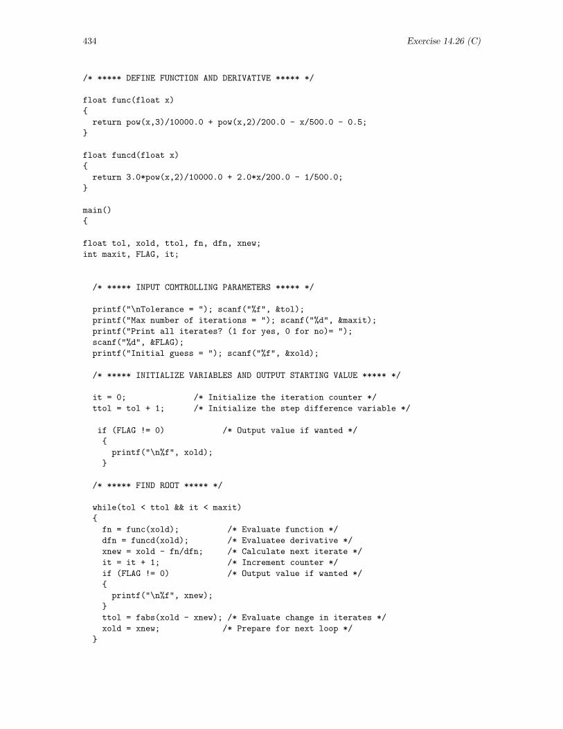
434 Exercise 14.26 (C)
/* ***** DEFINE FUNCTION AND DERIVATIVE ***** */
float func(float x)
return pow(x,3)/10000.0 + pow(x,2)/200.0 - x/500.0 - 0.5;
float funcd(float x)
return 3.0*pow(x,2)/10000.0 + 2.0*x/200.0 - 1/500.0;
main()
float tol, xold, ttol, fn, dfn, xnew;
int maxit, FLAG, it;
/* ***** INPUT COMTROLLING PARAMETERS ***** */
printf("\nTolerance = "); scanf("%f", &tol);
printf("Max number of iterations = "); scanf("%d", &maxit);
printf("Print all iterates? (1 for yes, 0 for no)= ");
scanf("%d", &FLAG);
printf("Initial guess = "); scanf("%f", &xold);
/* ***** INITIALIZE VARIABLES AND OUTPUT STARTING VALUE ***** */
it = 0; /* Initialize the iteration counter */
ttol = tol + 1; /* Initialize the step difference variable */
if (FLAG != 0) /* Output value if wanted */
printf("\n%f", xold);
/* ***** FIND ROOT ***** */
while(tol < ttol && it < maxit)
fn = func(xold); /* Evaluate function */
dfn = funcd(xold); /* Evaluatee derivative */
xnew = xold - fn/dfn; /* Calculate next iterate */
it = it + 1; /* Increment counter */
if (FLAG != 0) /* Output value if wanted */
printf("\n%f", xnew);
ttol = fabs(xold - xnew); /* Evaluate change in iterates */
xold = xnew; /* Prepare for next loop */
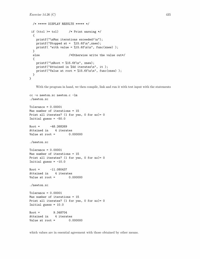
Exercise 14.26 (C) 435
/* ***** DISPLAY RESULTS ***** */
if (ttol >= tol) /* Print warning */
printf("\nMax iterations exceeded!\n");
printf("Stopped at = %15.6f\n",xnew);
printf( "with value = %15.6f\n\n", func(xnew) );
else /*Otherwise write the value out*/
printf("\nRoot = %15.6f\n", xnew);
printf("Attained in %4d iterates\n", it );
printf("Value at root = %15.6f\n\n", func(xnew) );
With the program in hand, we then compile, link and run it with test input with the statements
cc -o newton.xc newton.c -lm
./newton.xc
Tolerance = 0.00001
Max number of iterations = 15
Print all iterates? (1 for yes, 0 for no)= 0
Initial guess = -50.0
Root = -48.268269
Attained in 4 iterates
Value at root = 0.000000
./newton.xc
Tolerance = 0.00001
Max number of iterations = 15
Print all iterates? (1 for yes, 0 for no)= 0
Initial guess = -10.0
Root = -11.080437
Attained in 4 iterates
Value at root = 0.000000
./newton.xc
Tolerance = 0.00001
Max number of iterations = 15
Print all iterates? (1 for yes, 0 for no)= 0
Initial guess = 10.0
Root = 9.348704
Attained in 4 iterates
Value at root = 0.000000
which values are in essential agreement with those obtained by other means.
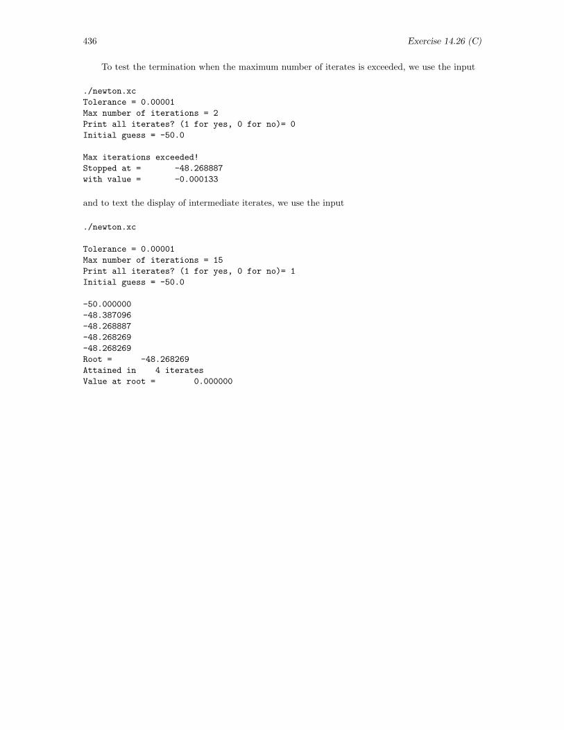
436 Exercise 14.26 (C)
To test the termination when the maximum number of iterates is exceeded, we use the input
./newton.xc
Tolerance = 0.00001
Max number of iterations = 2
Print all iterates? (1 for yes, 0 for no)= 0
Initial guess = -50.0
Max iterations exceeded!
Stopped at = -48.268887
with value = -0.000133
and to text the display of intermediate iterates, we use the input
./newton.xc
Tolerance = 0.00001
Max number of iterations = 15
Print all iterates? (1 for yes, 0 for no)= 1
Initial guess = -50.0
-50.000000
-48.387096
-48.268887
-48.268269
-48.268269
Root = -48.268269
Attained in 4 iterates
Value at root = 0.000000
Exercise 14.14 (NUMERICAL RECIPES-FORTRAN) 437
14.14 Natural Frequencies of Bar (NUMERICAL RECIPES-FORTRAN)
Exercise: The natural frequencies for the transverse vibrations of a bar of uniform cross sectionthat has length L and is free at both ends are given by
ωn =4K
L2
√E
ρα2n
where K is the radius of gyration of the cross section of the bar, E is Young’s modulus for thematerial of the bar, ρ is the density (mass/unit volume) of the material of the bar, and αn is asolution to the equation
tanα = ± tanhα
Find the lowest half dozen natural frequencies for this bar. [A detailed discussion of this exercise canbe found in N. H. Fletcher and T. D. Rossing, The Physics of Musical Instruments, Second Edition(Springer-Verlag, New York, 1991), pp. 57ff.]
Solution: The natural frequencies for the transverse vibrations of a bar of uniform cross sectionare given by the equation
ωn =4K
L2
√E
ρα2n
where L is the length of the bar, K is the radius of gyration of the cross-section of the bar, E isYoung’s modulus for the material of the bar, ρ is the density of the material of the bar, and αn is asolution to the equation
tan(α) = ± tanh(α)
Since K,L,E, and ρ are fixed for a given bar, the relationships among the natural frequencies ofthat bar are determined by αn. The previous equation can be rewritten as
tan(α)∓ tanh(α) = 0
Therefore, we can find the first six values of α2n, and thus the lowest half dozen natural frequencies
of the bar, by finding the roots of this equation and then squaring them.
As a start, we must have some idea where the roots we seek lie. Thus, graphs of the functionsy = tan(α) − tanh(α) and y = tan(α) + tanh(α) should be made. A graph of these functions ispresented in Fig. 14.23.7 From this graph we conclude that the first six roots lie in the intervals
tan(α) = − tanh(α) 2.0 < x < 3.0 5.2 < x < 6.0 8.0 < x < 9.0tan(α) = tanh(α) 3.5 < x < 4.5 6.5 < x < 7.5 10.0 < x < 10.7
You should use a program with which you are familiar to generate this—or an equivalent—graph.Note in particular that the divergences of the tangent function (1) complicate the production ofa graph that does not have extraneous and erroneous (nearly) vertical lines at α equal to an oddmultiple of π/2 and (2) make it critical to avoid embracing any of these special values of α in anyof the intervals in which we seek a root.
To find the roots of this equation, we choose first to use the Numerical Recipe rtbis.f,which we must copy to the default directory from the directory $NRHEAD/recipes_f/recipes. Asa start on a suitable driving program, we also copy the demonstration program xrtbis.f from$NRHEAD/recipes_f/demo/src, saving it under the name natfreq bisect.f. Then, we modify thedemonstration program in the following ways:
7FORTRAN by itself does not offer the possibility of making such graphs. The graph shown was produced byIDL. The coding used to create an equivalent graph in the program(s) incorporated in this document is recorded atthe end of this solution.
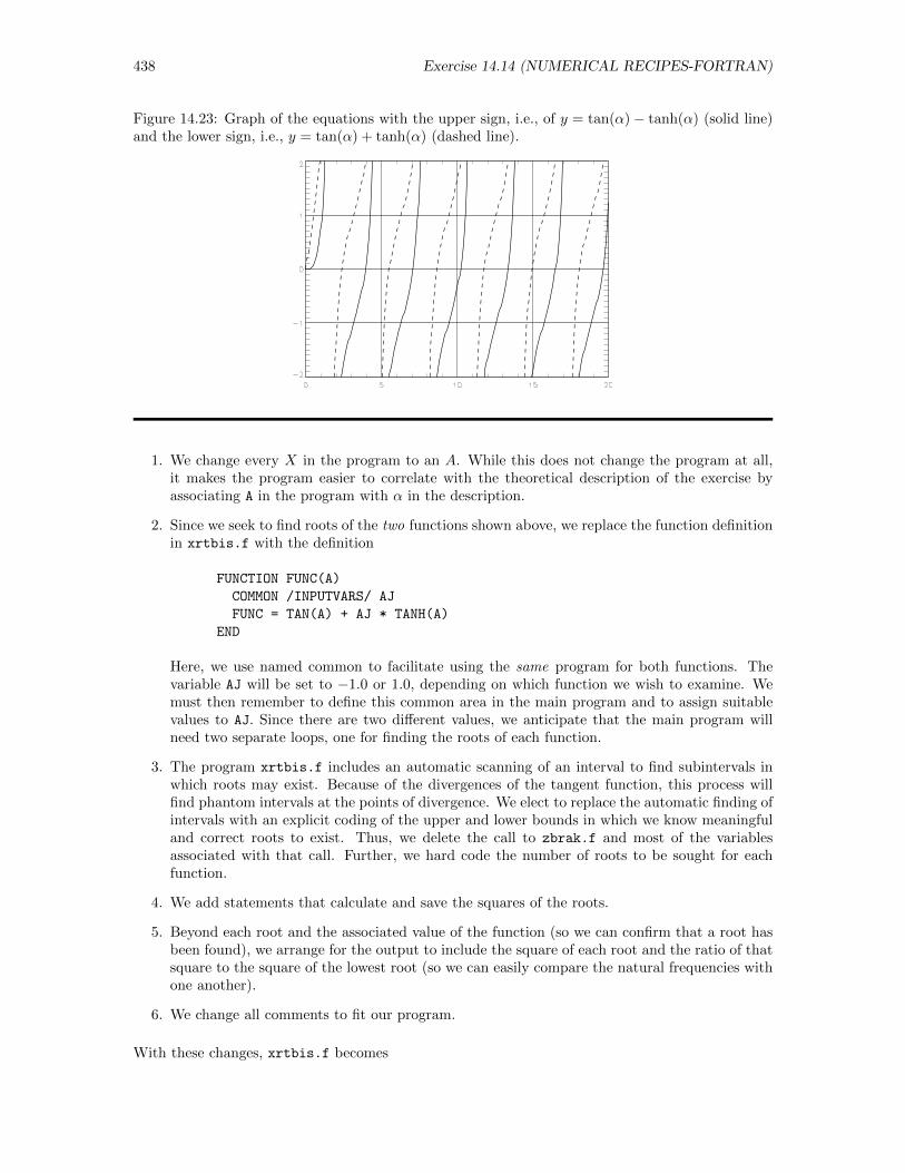
438 Exercise 14.14 (NUMERICAL RECIPES-FORTRAN)
Figure 14.23: Graph of the equations with the upper sign, i.e., of y = tan(α)− tanh(α) (solid line)and the lower sign, i.e., y = tan(α) + tanh(α) (dashed line).
1. We change every X in the program to an A. While this does not change the program at all,it makes the program easier to correlate with the theoretical description of the exercise byassociating A in the program with α in the description.
2. Since we seek to find roots of the two functions shown above, we replace the function definitionin xrtbis.f with the definition
FUNCTION FUNC(A)
COMMON /INPUTVARS/ AJ
FUNC = TAN(A) + AJ * TANH(A)
END
Here, we use named common to facilitate using the same program for both functions. Thevariable AJ will be set to −1.0 or 1.0, depending on which function we wish to examine. Wemust then remember to define this common area in the main program and to assign suitablevalues to AJ. Since there are two different values, we anticipate that the main program willneed two separate loops, one for finding the roots of each function.
3. The program xrtbis.f includes an automatic scanning of an interval to find subintervals inwhich roots may exist. Because of the divergences of the tangent function, this process willfind phantom intervals at the points of divergence. We elect to replace the automatic finding ofintervals with an explicit coding of the upper and lower bounds in which we know meaningfuland correct roots to exist. Thus, we delete the call to zbrak.f and most of the variablesassociated with that call. Further, we hard code the number of roots to be sought for eachfunction.
4. We add statements that calculate and save the squares of the roots.
5. Beyond each root and the associated value of the function (so we can confirm that a root hasbeen found), we arrange for the output to include the square of each root and the ratio of thatsquare to the square of the lowest root (so we can easily compare the natural frequencies withone another).
6. We change all comments to fit our program.
With these changes, xrtbis.f becomes
Exercise 14.14 (NUMERICAL RECIPES-FORTRAN) 439
PROGRAM NATFREQ_BISECT
EXTERNAL FUNC
DIMENSION AB1(3), AB2(3), SQ(6) ! For bounds and squares
COMMON /INPUTVARS/ AJ ! For selecting function
AACC = 1.0E-6 ! Set precision
AJ = 1.0 ! Set for tan(a)+tanh(a)
AB1(1) = 2.0 ! Set bounds
AB2(1) = 3.0
AB1(2) = 5.2
AB2(2) = 6.0
AB1(3) = 8.0
AB2(3) = 9.0
WRITE(*,’(1X,A)’) ’The roots of tan(a) + tanh(a) and their squares:’
WRITE(*,’(1X)’)
WRITE(*, 5) ’a’,’F(a)’,’a^2’, ’a^2/a1^2’
5 FORMAT( 1X,T19,A,T31,A,T45,A,T54,A )
WRITE(*,’(1X)’)
DO I = 1, 3 ! Find, save, display roots
ROOT = RTBIS( FUNC, AB1(I), AB2(I), AACC )
SQ(2*I-1) = ROOT**2
TMP = SQ(2*I-1)/SQ(1)
WRITE(*, 10) ’Root’, 2*I-1, ROOT, FUNC(ROOT), SQ(2*I-1), TMP
10 FORMAT( 1X,A,I2,2X,F12.6,E16.4,F12.6,F12.6 )
ENDDO
AJ = -1.0 ! Set for tan(a)-tanh(a)
AB1(1) = 3.5 ! Set bounds
AB2(1) = 4.5
AB1(2) = 6.5
AB2(2) = 7.5
AB1(3) = 10.0
AB2(3) = 10.7
WRITE(*,’(1X)’)
WRITE(*,’(1X,A)’) ’The roots of tan(a) - tanh(a) and their squares:’
WRITE(*,’(1X)’)
WRITE(*, 5) ’a’,’F(a)’,’a^2’, ’a^2/a1^2’
WRITE(*,’(1X)’)
DO I = 1, 3 ! Find, save, display roots
ROOT = RTBIS( FUNC, AB1(I), AB2(I), AACC )
SQ(2*I) = ROOT**2
TMP = SQ(2*I)/SQ(1)
WRITE(*, 10) ’Root’, 2*I, ROOT, FUNC(ROOT), SQ(2*I), TMP
ENDDO
END
FUNCTION FUNC(A) ! Define function
COMMON /INPUTVARS/ AJ
FUNC = TAN(A) + AJ * TANH(A)
END
Once this program and the recipe rtbis.f have been stored in the default directory, we compileand run the program with the statements
440 Exercise 14.14 (NUMERICAL RECIPES-FORTRAN)
f77 -o natfreq_bisect.xf natfreq_bisect.f rtbis.f
./natfreq_bisect.xf
The resulting output is
The roots of tan(a) + tanh(a) and their squares:
a F(a) a^2 a^2/a1^2
Root 1 2.365020 -0.1132E-05 5.593318 1.000000
Root 3 5.497804 -0.4768E-06 30.225845 5.403920
Root 5 8.639380 -0.6557E-06 74.638878 13.344293
The roots of tan(a) - tanh(a) and their squares:
a F(a) a^2 a^2/a1^2
Root 2 3.926601 -0.1848E-05 15.418199 2.756539
Root 4 7.068583 -0.4768E-06 49.964859 8.932955
Root 6 10.210176 -0.1252E-05 104.247681 18.637896
We conclude that the values of α2n that correspond to the lowest six natural frequencies are 5.593318,
15.418199, 30.225845, 49.964859, 74.638878, and 104.247681, though not all the digits reported aresignificant. Thus, we determine that the natural frequencies themselves are given by
ω1 = 5.5933184K
L2
√E
ρω2 = 15.418199
4K
L2
√E
ρ= 2.756539ω1
ω3 = 30.2258454K
L2
√E
ρ= 5.403920ω1 ω4 = 49.964859
4K
L2
√E
ρ= 8.932955ω1
ω5 = 74.6388784K
L2
√E
ρ= 13.344293ω1 ω6 = 104.247681
4K
L2
√E
ρ= 18.637896ω1
Similar edits to the demo program xrtnewt.f, though including recasting of FUNC to FUNCD—a subroutine that returns both the function and its first derivative, produces the programnatfreq newt.f:
PROGRAM NATFREQ_NEWT
EXTERNAL FUNCD
DIMENSION AB1(3), AB2(3), SQ(6) ! For bounds and squares
COMMON /INPUTVARS/ AJ ! For selecting function
AJ = 1.0 ! Set for tan(a)+tanh(a)
AB1(1) = 2.0 ! Set bounds
AB2(1) = 3.0
AB1(2) = 5.2
AB2(2) = 6.0
AB1(3) = 8.0
AB2(3) = 9.0
WRITE(*,’(1X,A)’) ’The roots of tan(a) + tanh(a) and their squares:’
WRITE(*,’(1X)’)
WRITE(*, 5) ’a’,’F(a)’,’a^2’, ’a^2/a1^2’
Exercise 14.14 (NUMERICAL RECIPES-FORTRAN) 441
5 FORMAT( 1X,T19,A,T31,A,T45,A,T54,A )
WRITE(*,’(1X)’)
DO I = 1, 3 ! Find, save, display roots
AACC=(1.0e-6)*(AB1(I)+AB2(I))/2.0
ROOT=RTNEWT( FUNCD, AB1(I), AB2(I), AACC )
SQ(2*I-1) = ROOT**2
TMP = SQ(2*I-1)/SQ(1)
CALL FUNCD( ROOT, FN, DF )
WRITE(*, 10) ’Root’, 2*I-1, ROOT, FN, SQ(2*I-1), TMP
10 FORMAT( 1X,A,I2,2X,F12.6,E16.4,F12.6,F12.6 )
ENDDO
AJ = -1.0 ! Set for tan(a)-tanh(a)
AB1(1) = 3.5 ! Set bounds
AB2(1) = 4.5
AB1(2) = 6.5
AB2(2) = 7.5
AB1(3) = 10.0
AB2(3) = 10.7
WRITE(*,’(1X)’)
WRITE(*,’(1X,A)’) ’The roots of tan(a) - tanh(a) and their squares:’
WRITE(*,’(1X)’)
WRITE(*, 5) ’a’,’F(a)’,’a^2’, ’a^2/a1^2’
WRITE(*,’(1X)’)
DO I = 1, 3 ! Find, save, display roots
AACC=(1.0e-6)*(AB1(I)+AB2(I))/2.0
ROOT=RTNEWT( FUNCD, AB1(I), AB2(I), AACC )
SQ(2*I) = ROOT**2
TMP = SQ(2*I)/SQ(1)
CALL FUNCD( ROOT, FN, DF )
WRITE(*, 10) ’Root’, 2*I, ROOT, FN, SQ(2*I), TMP
ENDDO
END
SUBROUTINE FUNCD( A, FN, DF ) ! Define subroutine
COMMON /INPUTVARS/ AJ
FN = TAN(A) + AJ * TANH(A)
DF = TAN(A)**2 - AJ*TANH(A)**2 + AJ+1.0
RETURN
END
This program uses the alternative recipe rtnewt.f and can be compiled, linked, and run with thestatements
f77 -o natfreq_newt.xf natfreq_newt.f rtnewt.f
./natfreq_newt.xf
The resulting output is
The roots of tan(a) + tanh(a) and their squares:
a F(a) a^2 a^2/a1^2
442 Exercise 14.14 (NUMERICAL RECIPES-FORTRAN)
Root 1 2.365020 -0.1788E-06 5.593321 1.000000
Root 3 5.497804 -0.4768E-06 30.225845 5.403918
Root 5 8.639380 -0.6557E-06 74.638878 13.344287
The roots of tan(a) - tanh(a) and their squares:
a F(a) a^2 a^2/a1^2
Root 2 3.926602 0.5960E-07 15.418206 2.756539
Root 4 7.068583 0.4768E-06 49.964867 8.932952
Root 6 10.210176 0.7153E-06 104.247704 18.637892
Within roundoff error, this output is entirely consistent with that produced by the first program.
IDL Code
; Establish independent and dependent variables
alpha = findgen(401)/20.0 ; 0.0 <= alpha <= 20.0, 0.05 increment
; 401 entries
y1 = tan(alpha) + tanh(alpha)
y2 = tan(alpha) - tanh(alpha)
; Determine indices at which functions diverge. They
; are the same for both y1 and y2.
for i = 0, 399 do $
if signum(y1[i]) eq 1 and signum(y1[i+1])eq -1 then print, i
; 31 94 157 219 282 345
ind = [ 31, 94, 157, 219, 282, 345, 402] ; Add 400+2 to final segment of graph
; Plot y1 and y2, avoiding the points of divergence by 2 entries
plot, alpha[0:30],y1[0:30], ticklen=1, linestyle=2, thick=3, $
xrange=[0.0,20.0], yrange=[-2.0,2.0]
oplot, alpha[0:30],y2[0:30], thick=3
for i = 0,5 do begin $
st=ind[i]+2 & en=ind[i+1]-2 & $
oplot, alpha[st:en],y1[st:en], linestyle=2, thick=3 & $
oplot, alpha[st:en],y2[st:en], thick=3 & $
end
Exercise 14.18 (NUMERICAL RECIPES-FORTRAN) 443
14.18 Single-Slit Diffraction (NUMERICAL RECIPES-FORTRAN)
Exercise: The intensity I(x) in the diffraction pattern produced by a single slit is given by
I(x)
I0=
sin2 x
x2
where I0 is the intensity in the center and x is related to the position of the observation point awayfrom the central maximum. The zeroes in this pattern are easy to locate (they occur at x = nπ,n = 0,±1,±2, . . .). Careful location of the maxima, however, is more complicated. They don’t occurwhere sin2 x = 1 because of the influence of the denominator that steadily increases as x increases.Locate the positions of the first half dozen maxima in this pattern, which—basically—is a requestto find the roots of the derivative of the function (though note that not all roots correspond tomaxima). Use at least three different methods and at least two different computational tools, andcompare the results. Do your results confirm that the roots approach odd multiples of 1
2π as theybecome large? Optional : You might also find it interesting to approximate the function with a powerseries expansion for sinx, keeping quite a few terms but converting the root finding problem intothat of finding the roots of a polynomial. Then, use methods for finding roots of polynomials andsee if you can come to understand how accuracy depends on how many terms you keep and whichroot you seek.
Solution: The intensity I(x) in the diffraction pattern produced by a single slit is given by
I(x)
I0=
sin2 x
x2
A graph of this function is given in Fig. 14.24.8 We seek the points at which this function has itsmaxima, i.e., the points at which
g(x) =d
dx
(sin2 x
x2
)=
2 sinx cosx
x2− 2 sin2 x
x3= 0
Using the FORTRAN version of Numerical Recipes routines to locate the roots of this equation isquite simple. For rtbis.f, we copy xrtbis.f into the default directory under a new name. Then,following the insight from the graph, we elect to find the roots of g(x) in the interval −0.5 ≤ x ≤ 20.0,so we modify our parameters to take us through the range. We must also tell the program thatwe are using an external function FUNC, which we define at the end to be the first derivative of ourintensity function. The resulting program follows is
PROGRAM EX18BIN
EXTERNAL FUNC
PARAMETER( N=150, NBMAX=20, X1=-0.5, X2=20.0 )
DIMENSION XB1(NBMAX), XB2(NBMAX)
NB=NBMAX
CALL ZBRAK( FUNC, X1, X2, N, XB1, XB2, NB )
WRITE(*,’(/1X,T19,A,T31,A/)’) ’x’, ’F(x)’
DO I = 1, NB
XACC = 1.0E-6
ROOT = RTBIS( FUNC,XB1(I), XB2(I), XACC )
WRITE( *, ’(1X,A,I2,2X,F12.6,E16.4)’) ’Root ’, I, ROOT,
+ FUNC(ROOT)
8FORTRAN by itself does not offer the possibility of making such graphs. The graph shown was produced byIDL. The coding used to create an equivalent graph in the program(s) incorporated in this document is recorded atthe end of this solution.
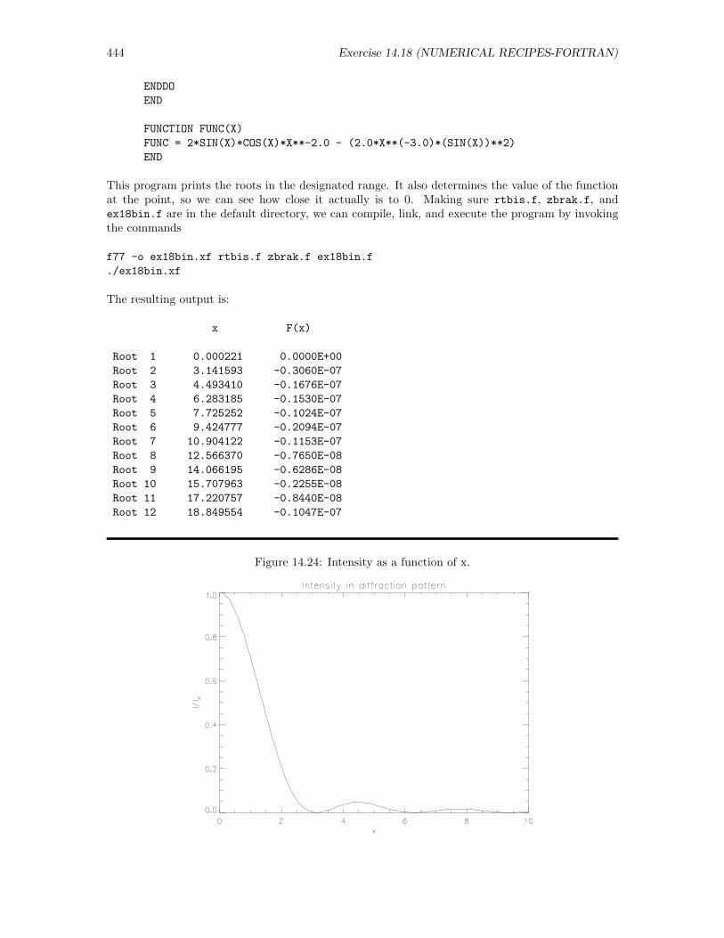
444 Exercise 14.18 (NUMERICAL RECIPES-FORTRAN)
ENDDO
END
FUNCTION FUNC(X)
FUNC = 2*SIN(X)*COS(X)*X**-2.0 - (2.0*X**(-3.0)*(SIN(X))**2)
END
This program prints the roots in the designated range. It also determines the value of the functionat the point, so we can see how close it actually is to 0. Making sure rtbis.f, zbrak.f, andex18bin.f are in the default directory, we can compile, link, and execute the program by invokingthe commands
f77 -o ex18bin.xf rtbis.f zbrak.f ex18bin.f
./ex18bin.xf
The resulting output is:
x F(x)
Root 1 0.000221 0.0000E+00
Root 2 3.141593 -0.3060E-07
Root 3 4.493410 -0.1676E-07
Root 4 6.283185 -0.1530E-07
Root 5 7.725252 -0.1024E-07
Root 6 9.424777 -0.2094E-07
Root 7 10.904122 -0.1153E-07
Root 8 12.566370 -0.7650E-08
Root 9 14.066195 -0.6286E-08
Root 10 15.707963 -0.2255E-08
Root 11 17.220757 -0.8440E-08
Root 12 18.849554 -0.1047E-07
Figure 14.24: Intensity as a function of x.
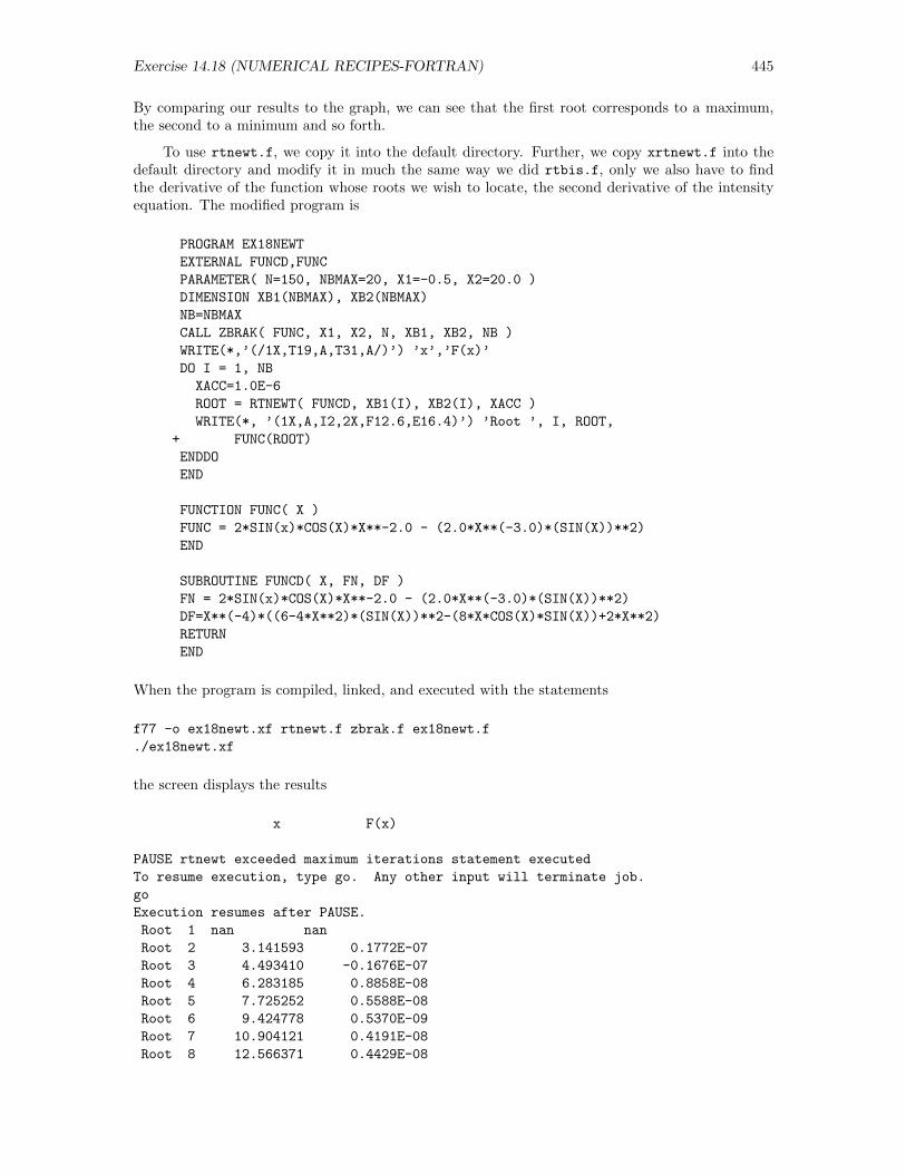
Exercise 14.18 (NUMERICAL RECIPES-FORTRAN) 445
By comparing our results to the graph, we can see that the first root corresponds to a maximum,the second to a minimum and so forth.
To use rtnewt.f, we copy it into the default directory. Further, we copy xrtnewt.f into thedefault directory and modify it in much the same way we did rtbis.f, only we also have to findthe derivative of the function whose roots we wish to locate, the second derivative of the intensityequation. The modified program is
PROGRAM EX18NEWT
EXTERNAL FUNCD,FUNC
PARAMETER( N=150, NBMAX=20, X1=-0.5, X2=20.0 )
DIMENSION XB1(NBMAX), XB2(NBMAX)
NB=NBMAX
CALL ZBRAK( FUNC, X1, X2, N, XB1, XB2, NB )
WRITE(*,’(/1X,T19,A,T31,A/)’) ’x’,’F(x)’
DO I = 1, NB
XACC=1.0E-6
ROOT = RTNEWT( FUNCD, XB1(I), XB2(I), XACC )
WRITE(*, ’(1X,A,I2,2X,F12.6,E16.4)’) ’Root ’, I, ROOT,
+ FUNC(ROOT)
ENDDO
END
FUNCTION FUNC( X )
FUNC = 2*SIN(x)*COS(X)*X**-2.0 - (2.0*X**(-3.0)*(SIN(X))**2)
END
SUBROUTINE FUNCD( X, FN, DF )
FN = 2*SIN(x)*COS(X)*X**-2.0 - (2.0*X**(-3.0)*(SIN(X))**2)
DF=X**(-4)*((6-4*X**2)*(SIN(X))**2-(8*X*COS(X)*SIN(X))+2*X**2)
RETURN
END
When the program is compiled, linked, and executed with the statements
f77 -o ex18newt.xf rtnewt.f zbrak.f ex18newt.f
./ex18newt.xf
the screen displays the results
x F(x)
PAUSE rtnewt exceeded maximum iterations statement executed
To resume execution, type go. Any other input will terminate job.
go
Execution resumes after PAUSE.
Root 1 nan nan
Root 2 3.141593 0.1772E-07
Root 3 4.493410 -0.1676E-07
Root 4 6.283185 0.8858E-08
Root 5 7.725252 0.5588E-08
Root 6 9.424778 0.5370E-09
Root 7 10.904121 0.4191E-08
Root 8 12.566371 0.4429E-08
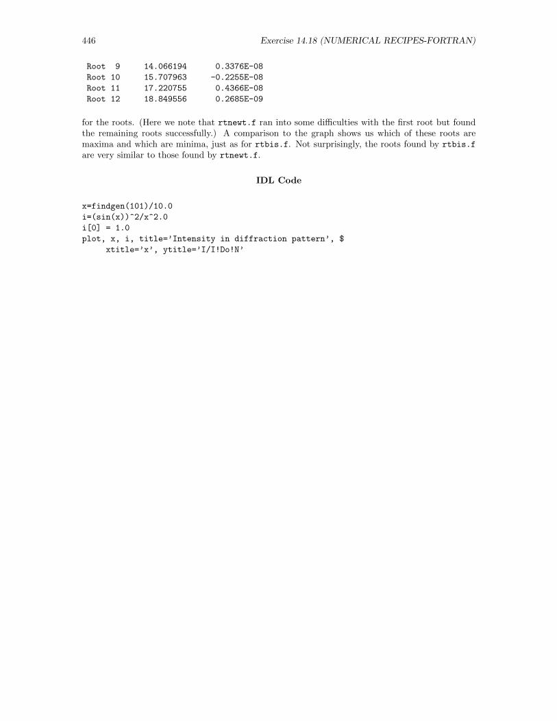
446 Exercise 14.18 (NUMERICAL RECIPES-FORTRAN)
Root 9 14.066194 0.3376E-08
Root 10 15.707963 -0.2255E-08
Root 11 17.220755 0.4366E-08
Root 12 18.849556 0.2685E-09
for the roots. (Here we note that rtnewt.f ran into some difficulties with the first root but foundthe remaining roots successfully.) A comparison to the graph shows us which of these roots aremaxima and which are minima, just as for rtbis.f. Not surprisingly, the roots found by rtbis.f
are very similar to those found by rtnewt.f.
IDL Code
x=findgen(101)/10.0
i=(sin(x))^2/x^2.0
i[0] = 1.0
plot, x, i, title=’Intensity in diffraction pattern’, $
xtitle=’x’, ytitle=’I/I!Do!N’
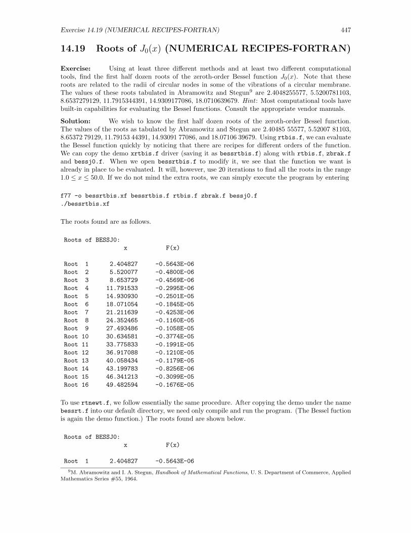
Exercise 14.19 (NUMERICAL RECIPES-FORTRAN) 447
14.19 Roots of J0(x) (NUMERICAL RECIPES-FORTRAN)
Exercise: Using at least three different methods and at least two different computationaltools, find the first half dozen roots of the zeroth-order Bessel function J0(x). Note that theseroots are related to the radii of circular nodes in some of the vibrations of a circular membrane.The values of these roots tabulated in Abramowitz and Stegun9 are 2.4048255577, 5.5200781103,8.6537279129, 11.7915344391, 14.9309177086, 18.0710639679. Hint : Most computational tools havebuilt-in capabilities for evaluating the Bessel functions. Consult the appropriate vendor manuals.
Solution: We wish to know the first half dozen roots of the zeroth-order Bessel function.The values of the roots as tabulated by Abramowitz and Stegun are 2.40485 55577, 5.52007 81103,8.65372 79129, 11.79153 44391, 14.93091 77086, and 18.07106 39679. Using rtbis.f, we can evaluatethe Bessel function quickly by noticing that there are recipes for different orders of the function.We can copy the demo xrtbis.f driver (saving it as bessrtbis.f) along with rtbis.f, zbrak.fand bessj0.f. When we open bessrtbis.f to modify it, we see that the function we want isalready in place to be evaluated. It will, however, use 20 iterations to find all the roots in the range1.0 ≤ x ≤ 50.0. If we do not mind the extra roots, we can simply execute the program by entering
f77 -o bessrtbis.xf bessrtbis.f rtbis.f zbrak.f bessj0.f
./bessrtbis.xf
The roots found are as follows.
Roots of BESSJ0:
x F(x)
Root 1 2.404827 -0.5643E-06
Root 2 5.520077 -0.4800E-06
Root 3 8.653729 -0.4569E-06
Root 4 11.791533 -0.2995E-06
Root 5 14.930930 -0.2501E-05
Root 6 18.071054 -0.1845E-05
Root 7 21.211639 -0.4253E-06
Root 8 24.352465 -0.1160E-05
Root 9 27.493486 -0.1058E-05
Root 10 30.634581 -0.3774E-05
Root 11 33.775833 -0.1991E-05
Root 12 36.917088 -0.1210E-05
Root 13 40.058434 -0.1179E-05
Root 14 43.199783 -0.8256E-06
Root 15 46.341213 -0.3099E-05
Root 16 49.482594 -0.1676E-05
To use rtnewt.f, we follow essentially the same procedure. After copying the demo under the namebessrt.f into our default directory, we need only compile and run the program. (The Bessel fuctionis again the demo function.) The roots found are shown below.
Roots of BESSJ0:
x F(x)
Root 1 2.404827 -0.5643E-06
9M. Abramowitz and I. A. Stegun, Handbook of Mathematical Functions, U. S. Department of Commerce, AppliedMathematics Series #55, 1964.
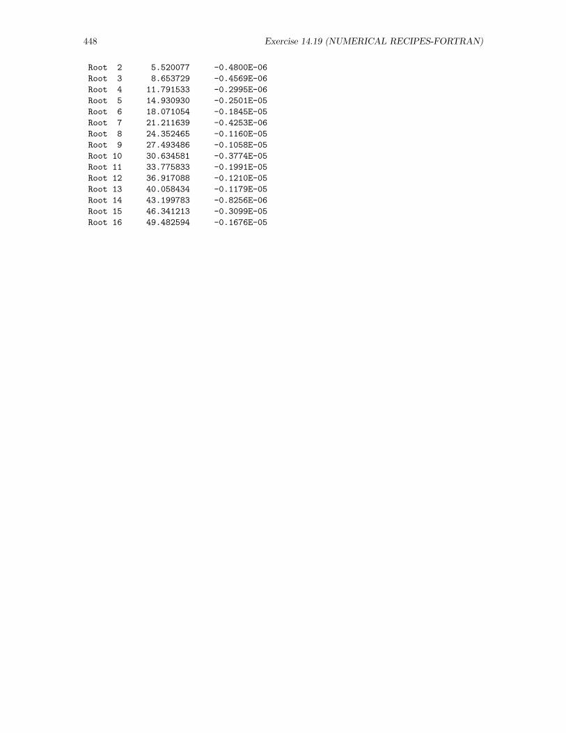
448 Exercise 14.19 (NUMERICAL RECIPES-FORTRAN)
Root 2 5.520077 -0.4800E-06
Root 3 8.653729 -0.4569E-06
Root 4 11.791533 -0.2995E-06
Root 5 14.930930 -0.2501E-05
Root 6 18.071054 -0.1845E-05
Root 7 21.211639 -0.4253E-06
Root 8 24.352465 -0.1160E-05
Root 9 27.493486 -0.1058E-05
Root 10 30.634581 -0.3774E-05
Root 11 33.775833 -0.1991E-05
Root 12 36.917088 -0.1210E-05
Root 13 40.058434 -0.1179E-05
Root 14 43.199783 -0.8256E-06
Root 15 46.341213 -0.3099E-05
Root 16 49.482594 -0.1676E-05
Exercise 14.20 (NUMERICAL RECIPES-FORTRAN) 449
14.20 Double-Welled Potential (NUMERICAL RECIPES-FORTRAN)
Exercise: Suppose a particle moves in one dimension under the influence of the potentialenergy
V (x) =−V0a
2(a2 + x2)
8a4 + x4=⇒ V (x)
V0= − (1 + x2)
8 + x4
where x = x/a. Using at least three different methods and at least two different computational tools,find the coordinates x of all turning points when the total energy E of the particle is E = −0.2V0
and also when the total energy is E = −0.1V0. Optional : Obtain graphs of the position of eachturning point as a function of particle energy over the allowed range of energies for bound states.
Solution: We can examine the one-dimensional motion of a particle under the influence of apotential energy
V (x)
V0= −1 +X2
8 +X4
We wish to know the coordinates of all the turning points when the total energy E is E = −0.1V0
as well as when E = −0.2V0. To do this we must find the roots of the equations
V1 = 0.1− 1 +X2
8 +X4and V2 = 0.2− 1 +X2
8 +X4
respectively. (At the roots, the kinetic energy K will be K = 0.) We can find the roots of ourequations in FORTRAN using the Numerical Recipes rtbis.f and rtnewt.f. To use rtbis.f, wemust copy the file xrtbis.f into our default directory under a new name. Knowing that the rootsfor V1 lie in the range −4.0 ≤ x ≤ 4.0, we modify the range in the program. We need also modifythe definition of the function to conform with V1. The resulting program is
PROGRAM XRTBIS
EXTERNAL FUNC
PARAMETER(N=100,NBMAX=20,X1=-4.0,X2=4.0)
DIMENSION XB1(NBMAX),XB2(NBMAX)
NB=NBMAX
CALL ZBRAK(FUNC,X1,X2,N,XB1,XB2,NB)
WRITE(*,’(/1X,A)’) ’Roots of FUNC:’
WRITE(*,’(/1X,T19,A,T31,A/)’) ’x’,’F(x)’
DO I=1,NB
XACC=(1.0E-6)
ROOT=RTBIS(FUNC,XB1(I),XB2(I),XACC)
WRITE(*,’(1X,A,I2,2X,F12.6,E16.4)’) ’Root ’,I,ROOT,FUNC(ROOT)
ENDDO
END
FUNCTION FUNC(X)
FUNC=0.1-((X**2+1.0)/(X**4+8.0))
END
After copying the files rtbis.f and zbrak.f from the Numerical Recipes directory, we compile andrun the program with the statements
f77 -o xrtbis.xf xrtbis.f rtbis.f zbrak.f
./xrtbis.xf
The resulting output is
450 Exercise 14.20 (NUMERICAL RECIPES-FORTRAN)
Roots of FUNC:
x F(x)
Root 1 -3.193141 -0.3725E-07
Root 2 3.193141 -0.3725E-07
To find the roots of V2, we need only adjust the function FUNC to read FUNC = 0.2- .... The resultof running the program with that modification is
Roots of FUNC:
x F(x)
Root 1 -2.074313 0.0000E+00
Root 2 -0.835000 -0.8941E-07
Root 3 0.835000 -0.7451E-07
Root 4 2.074313 0.0000E+00
If we wish to use rtnewt instead, we must supply not only the function but also its derivative.For both total energies, we have
V ′1 = V ′2 =2X5 + 4X3 − 16X
X8 + 16X4 + 64
After copying xrtnewt.f into our default directory, we modify it by changing the range (as forxrtbis.f) and entering the function and its derivative. The modified program looks is
PROGRAM XRTNEWT
EXTERNAL FUNCD, FUNC
PARAMETER(N=100,NBMAX=20,X1=-4.0,X2=4.0)
DIMENSION XB1(NBMAX),XB2(NBMAX)
NB=NBMAX
CALL ZBRAK(FUNC,X1,X2,N,XB1,XB2,NB)
WRITE(*,’(/1X,A)’) ’Roots of FUNC:’
WRITE(*,’(/1X,T19,A,T31,A/)’) ’x’,’F(x)’
DO I=1,NB
XACC=(1.0E-6)
ROOT=RTNEWT(FUNCD,XB1(I),XB2(I),XACC)
WRITE(*,’(1X,A,I2,2X,F12.6,E16.4)’) ’Root ’,I,ROOT,FUNC(ROOT)
ENDDO
END
FUNCTION FUNC(x)
FUNC=0.1-((X**2+1.0)/(X**4+8.0))
END
SUBROUTINE FUNCD(X,FN,DF)
FN=0.1-((X**2+1.0)/(X**4+8.0))
DF=(2.0*X**5+4.0*X**3-16.0*X)/(X**8+16.0*X**4+64)
RETURN
END
To run this program, we make sure all of the supporting files are in our directory, then type
f77 -o xrtnewt.xf rtnewt.f zbrak.f polint.f xrtnewt.f
./xrtnewt.xf
Exercise 14.20 (NUMERICAL RECIPES-FORTRAN) 451
The program returns the roots
Roots of FUNC:
x F(x)
Root 1 -3.193141 -0.7451E-08
Root 2 3.193141 -0.7451E-08
for V1 To find the roots of V2, we make the same single adjustment as we did for xrtbis.f (bothunder FUNCTION and SUBROUTINE), recalling the the derivatives of the two functions are the same.Compiling and running this modified program yields the result
Roots of FUNC:
x F(x)
Root 1 -2.074313 0.0000E+00
Root 2 -0.835000 -0.1490E-07
Root 3 0.835000 -0.1490E-07
Root 4 2.074313 0.0000E+00
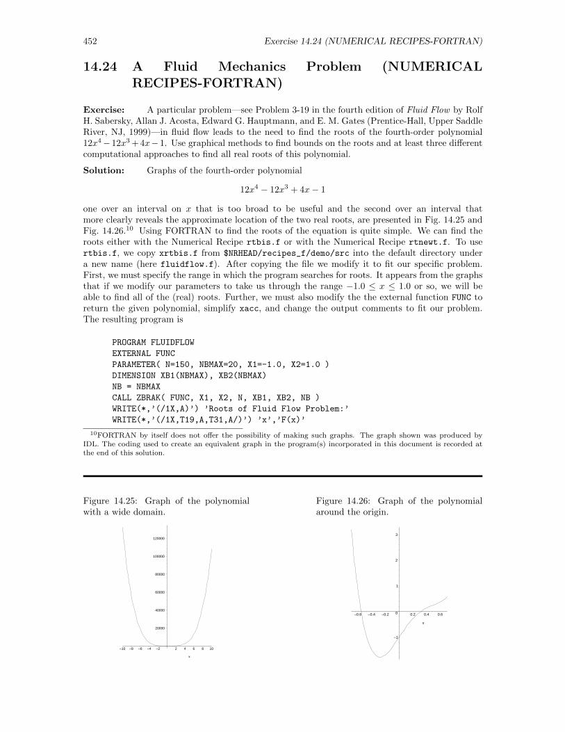
452 Exercise 14.24 (NUMERICAL RECIPES-FORTRAN)
14.24 A Fluid Mechanics Problem (NUMERICALRECIPES-FORTRAN)
Exercise: A particular problem—see Problem 3-19 in the fourth edition of Fluid Flow by RolfH. Sabersky, Allan J. Acosta, Edward G. Hauptmann, and E. M. Gates (Prentice-Hall, Upper SaddleRiver, NJ, 1999)—in fluid flow leads to the need to find the roots of the fourth-order polynomial12x4−12x3 + 4x−1. Use graphical methods to find bounds on the roots and at least three differentcomputational approaches to find all real roots of this polynomial.
Solution: Graphs of the fourth-order polynomial
12x4 − 12x3 + 4x− 1
one over an interval on x that is too broad to be useful and the second over an interval thatmore clearly reveals the approximate location of the two real roots, are presented in Fig. 14.25 andFig. 14.26.10 Using FORTRAN to find the roots of the equation is quite simple. We can find theroots either with the Numerical Recipe rtbis.f or with the Numerical Recipe rtnewt.f. To usertbis.f, we copy xrtbis.f from $NRHEAD/recipes_f/demo/src into the default directory undera new name (here fluidflow.f). After copying the file we modify it to fit our specific problem.First, we must specify the range in which the program searches for roots. It appears from the graphsthat if we modify our parameters to take us through the range −1.0 ≤ x ≤ 1.0 or so, we will beable to find all of the (real) roots. Further, we must also modify the the external function FUNC toreturn the given polynomial, simplify xacc, and change the output comments to fit our problem.The resulting program is
PROGRAM FLUIDFLOW
EXTERNAL FUNC
PARAMETER( N=150, NBMAX=20, X1=-1.0, X2=1.0 )
DIMENSION XB1(NBMAX), XB2(NBMAX)
NB = NBMAX
CALL ZBRAK( FUNC, X1, X2, N, XB1, XB2, NB )
WRITE(*,’(/1X,A)’) ’Roots of Fluid Flow Problem:’
WRITE(*,’(/1X,T19,A,T31,A/)’) ’x’,’F(x)’
10FORTRAN by itself does not offer the possibility of making such graphs. The graph shown was produced byIDL. The coding used to create an equivalent graph in the program(s) incorporated in this document is recorded atthe end of this solution.
Figure 14.25: Graph of the polynomialwith a wide domain.
20000
40000
60000
80000
100000
120000
–10 –8 –6 –4 –2 2 4 6 8 10
x
Figure 14.26: Graph of the polynomialaround the origin.
–1
0
1
2
3
–0.6 –0.4 –0.2 0.2 0.4 0.6
x
Exercise 14.24 (NUMERICAL RECIPES-FORTRAN) 453
DO I = 1, NB
XACC=1.0E-6
ROOT = RTBIS(FUNC,XB1(I),XB2(I),XACC)
WRITE(*,’(1X,A,I2,2X,F12.6,E16.4)’) ’Root ’,I,ROOT,FUNC(ROOT)
ENDDO
END
FUNCTION FUNC(X)
FUNC = 12.0*X**4 - 12.0*X**3 + 4.0*X - 1.0
END
Finally, we must copy the files rtbis.f and zbrak.f from $NRHEAD/recipes_f/recipes into thedefault directory. Then, we compile fluidflow.f (along with rtbis.f and zbrak.f) and link theprogram with the statement
f77 -o fluidflow.xf fluidflow.f rtbis.f zbrak.f
and finally run the program with the statement
./fluidflow.xf
Roots of Fluid Flow Problem:
x F(x)
Root 1 -0.556950 -0.1121E-04
Root 2 0.313409 -0.1431E-05
To use rtnewt.f, we follow essentially the same procedure. Assuming that we already havezbrak.f in the default directory, we only have to copy two files. First, we copy the file rtnewt.f
from $NRHEAD/recipes_f/recipes into our default directory. Second, we copy the file xrtnewt.f
from $NRHEAD/recipes_c-ansi/demo/src (saving it under the name fluidnewt.f) into the defaultdirectory. We modify fluidnewt.f in much the same way we modified the original version offluidflow.f, first, changing the parameters to scan through the range −1.0 ≤ x ≤ 1.0, thenmodifying the external function FUNC to return the given polynomial, simplifying xacc, and changingthe comment labeling the output. In addition, we enter the given polynomial and its derivative intothe subroutine FUNCD. The resulting program is
PROGRAM FLUIDNEWT
EXTERNAL FUNCD, FUNC
PARAMETER( N=100, NBMAX=20, X1=-1.0, X2=1.0 )
DIMENSION XB1(NBMAX), XB2(NBMAX)
NB = NBMAX
CALL ZBRAK( FUNC, X1, X2, N, XB1, XB2, NB )
WRITE(*,’(/1X,A)’) ’Roots of Fluid Flow Problem:’
WRITE(*,’(/1X,T19,A,T31,A/)’) ’x’,’F(x)’
DO I=1,NB
XACC = 1.0E-6
ROOT = RTNEWT(FUNCD,XB1(I),XB2(I),XACC)
WRITE(*,’(1X,A,I2,2X,F12.6,E16.4)’) ’Root ’,I,ROOT,FUNC(ROOT)
ENDDO
END
454 Exercise 14.24 (NUMERICAL RECIPES-FORTRAN)
FUNCTION FUNC(X)
FUNC = 12.0*X**4 - 12.0*X**3 + 4.0*X - 1.0
END
SUBROUTINE FUNCD(X,FN,DF)
FN = 12.0*X**4 - 12.0*X**3 + 4.0*X - 1.0
DF = 48.0*X**3 - 36.0*X**2 + 4.0
RETURN
END
Having already copied the necessary files to our default directory, we compile, link, and execute theprogram with the statements
f77 -o fluidnewt.xf fluidnewt.f rtnewt.f zbrak.f
./fluidnewt.xf
Roots of Fluid Flow Problem:
x F(x)
Root 1 -0.556951 -0.2384E-06
Root 2 0.313410 0.0000E+00
From both programs we see that the two roots of the given fourth-order polynomial are−0.556951 and 0.313410.
IDL Code
x= -10.0 + 20.0*findgen(201)/200.0
y = 12.0*x^4 - 12.0*x^3+ 4.0*x-1.0
plot, x, y, thick=4
oplot, [-10.0, 10.0], [0.0,0.0], linestyle=2
x= -1.0 + 2.0*findgen(101)/100.0
y = 12.0*x^4 - 12.0*x^3+ 4.0*x-1.0
plot, x, y, thick=4
oplot, [-1.0, 1.0], [0.0,0.0], linestyle=2
Exercise 14.29 (NUMERICAL RECIPES-FORTRAN) 455
14.29 Finite Depth Square Well (NUMERICAL RECIPES-FORTRAN)
Exercise: Study the demonstration programs xrtbis.f and xrtnewt.f, each of which iswritten so as to be able to find all roots of a given function in a specified range. Then recast eachof these programs to produce a program that will find all of the positive roots of the equation foreach sign in the equations
sin s = ±0.04 s or sin s∓ 0.04 s = 0
describing a finite-depth square well. Write your program so that the value of c and the boundariesof the region in which roots are to be sought are entered from the terminal at the time the programis run. Finally, test your program with c = 25, comparing your results with those obtained in thetext, and then examine other values of c, seeking ultimately to obtain a graph showing each root asa function of c.
Solution: We examine the way that the energy levels of a quantum well change as the depthand width of the well (specified by c) change. As described in CPSUP Section 12.1.5, the value ofs for an allowed energy level must satisfy the equation
s cot(s) = −√c2 − s2
We can simplify this equation, as is done in Section 12.1.5, by squaring it, finding that the values ofs for allowed energy levels are the roots of the expression
sin(s)∓ s
c= 0
Note however that, by simplifying the expression, we have possibly introduced spurious roots, so wemust ultimately check the roots in the original equation.
We can find the roots of our equation in FORTRAN using either the Numerical Recipe rtbis.fand a corresponding driving program or the Numerical Recipe rtnewt.f and a corresponding drivingprogram.
Solution using rtbis.f:
To use rtbis.f, we must copy several files into our default directory. First, we copy the demon-stration program xrtbis.f from $NRHEAD/recipes_f/demo/src and save it under an appropriatename (here qwell.f). Then, we modify this file to fit our specific problem by
• changing all variables whose names begin with X to variables with names beginning with S (soas to facilitate correlation of the program with the statement of the problem).
• defining the function whose roots are to be found with the statements
FUNCTION FUNC(S)
COMMON /INPUTVARS/ AJ, C
FUNC = SIN(S) + AJ*S/C
END
where we have introduced the variable AJ, which will be given the value +1 or the value −1as a means to combine both signs in the above equation into a single program, and we haveused named common to communicate both the value of AJ and the value of C to the functionsubprogram. For this function to work properly, we must then also add the statement
COMMON /INPUTVARS/ AJ, C
456 Exercise 14.29 (NUMERICAL RECIPES-FORTRAN)
to the compiler directives in the main program. Further, we add the statements
WRITE(*, ’(1X,A)’) ’Enter a value for c = ’
READ(*, *) C
WRITE(*, *) ’Enter -1 for an upper solution and 1 for a lower’
WRITE(*, *) ’solution =’
READ(*, *) AJ
to the main program so that values of C and AJ can be entered at execution time.
• deleting the arguments S1 and S2 of the PARAMETERS() directive that specify the range of thesearch and adding the statements
WRITE(*, ’(1X,A)’) ’Enter a value for the lower bound = ’
READ(*, *) S1
WRITE(*, ’(1X,A)’) ’Enter a value for the upper bound = ’
READ(*, *) S2
so that the range will be specified by the user at execution time. (Note that a search startedat the value s = 0 will generate an error message. We seek only positive roots, but we will,when the time comes, start each search at s = −0.5 to avoid the problem just mentioned.)
• arranging for writing the results into a file for transfer to a graphing program by defining thecharacter variable FILENAME and reading its value at execution time with the statements
CHARACTER*20 FILENAME
WRITE(*, *) ’Enter an appropriate file name(ends in .dat’
WRITE(*, *) ’and is less than 20 characters):’
READ(*, FMT=’(A)’) FILENAME
OPEN(UNIT=1, FILE = FILENAME, STATUS = ’NEW’)
We must, of course, also modify the output statement to write to this file rather than to thescreen and then, after all output has been produced, we must close the file.
These provisions allow the user to run the program multiple times without having to recompile it.The resulting program is
PROGRAM QWELL
EXTERNAL FUNC
CHARACTER*20 NAME
PARAMETER( N=100, NBMAX=20 )
DIMENSION SB1(NBMAX), SB2(NBMAX)
COMMON /INPUTVARS/ AJ, C
NB=NBMAX
WRITE(*, ’(1X,A)’) ’Enter a value for the lower bound: ’
READ(*, *) S1
WRITE(*, ’(1X,A)’) ’Enter a value for the upper bound: ’
READ(*, *) S2
WRITE(*, ’(1X,A)’) ’Enter a value for c: ’
READ(*, *) C
WRITE(*, *) ’Enter -1 for an upper solution and 1 for a lower’
WRITE(*, *) ’solution: ’
READ(*, *) AJ
Exercise 14.29 (NUMERICAL RECIPES-FORTRAN) 457
WRITE(*, *) ’Enter an appropriate file name(ends in .dat’
WRITE(*, *) ’ and is less than 20 characters): ’
READ(*, FMT=’(A)’) NAME
CALL ZBRAK(FUNC,S1,S2,N,SB1,SB2,NB)
OPEN(UNIT=1, FILE = NAME, STATUS = ’NEW’)
DO I=1,NB
SACC=(1.0E-6)
ROOT = RTBIS(FUNC,SB1(I),SB2(I),SACC)
WRITE(1,’(F12.6)’) ROOT
ENDDO
CLOSE( UNIT=1 )
END
FUNCTION FUNC(S)
COMMON /INPUTVARS/ AJ, C
FUNC = SIN(S) + AJ*S/C
END
Finally, we must copy the files rtbis.f and zbrak.f from $NRHEAD/recipes_f/recipes into ourdefault directory and compile qwell.f (along with rtbis.f and zbrak.f) with the statement
f77 -o qwell.xf qwell.f rtbis.f zbrak.f
Once the executable file qwell.xf is available, we run the program many times with differentvalues of c and different filenames. For example, with c = 2.0, we would create files containing theroots for each sign with the input
./qwell.xf
Enter a value for the lower bound: -0.5
Enter a value for the upper bound: 60.0
Enter a value for c: 2.0
Enter -1 for an upper solution and 1 for a lower solution: -1
Enter an appropriate file name(ends in .dat
and is less than 20 characters): qwell02up_f.dat
./qwell.xf
Enter a value for the lower bound: -0.5
Enter a value for the upper bound: 60.0
Enter a value for c: 2.0
Enter -1 for an upper solution and 1 for a lower solution: 1
Enter an appropriate file name(ends in .dat
and is less than 20 characters): qwell02lo_f.dat
In similar fashion, We run the program many times to obtain the results for several values of c,including c = 5, 10, 25, and 50. Each time we run the program we enter a different filename as theoutput location for the data, changing in particular the sixth and seventh characters to reflect thevalue of c to which the file applies. In particular, by displaying these files, we find that the roots(some of which are spurious) for c = 2 are
upper: 0.000000 lower: 0.000000
1.89549
458 Exercise 14.29 (NUMERICAL RECIPES-FORTRAN)
and those for c = 25 are
upper: 0.000000 lower: 0.000000
3.020478 3.272885
6.548204 6.039204
9.054186 9.828837
13.118793 12.062847
15.061390 16.424786
19.761087 18.043257
20.994287 23.177780
23.864494
Graphing Solution with IDL
To create the energy level diagram with IDL, we begin by opening our file and storing the datain an array with the statements
IDL> openr, 1, ’qwell02up_f.dat’
IDL> upper2 = fltarr(2,1)
IDL> readf, 1, upper2
IDL> close, 1
IDL> print, upper2
-1.00000e-06 1.89550
where qwell02up_f.dat is the name of the file where our data are stored. Note that we executethe statements for c = 2 to begin with. This is a special case and a more general routine appearsjust after this specific routine. We do not open the qwell02lo_f.dat file in IDL because we knowthat the only root in that file is zero and we know that it is a spurious root. However, for all othersubsequent routines (as shown later) we will also open the lower solution file. Furthermore, notethat the size of the array needed to store the data will vary for the upper and lower solutions as wellas for each value of c. To find the appropriate size for the array, the data file must be opened andlooked at. After creating the arrays in IDL we want to combine the upper and lower solutions as wellas weed out the spurious solutions. We begin by eliminating the spurious solutions. To accomplishthis task we plug the solutions back into the equation
s cot(s) = −√c2 − s2
with the statement
IDL> print, upper2*cos(upper2)/sin(upper2) + sqrt(2.0^2 -upper2^2)
3.00000 -4.29153e-06
Only those roots which produce a result of zero (within the precision of our determination of theroot) are acceptable solutions. We then combine the acceptable upper and lower solutions into asingle array and plug that array into the equation for E/V0
E/V0 = −(1− s2/c2)
to find the energies associated with the roots which is what we are actually interested in. Weaccomplish these tasks with the statements11
IDL> s2 = upper2[1]
IDL> energy2 = -(1 - s2^2/2.0^2)
IDL> print, energy2
-0.101775
11Note that the statements used to accomplish the merging of the two separate solutions are different for smallvalues of c, but follow the form used for c = 25 for larger values of c
Exercise 14.29 (NUMERICAL RECIPES-FORTRAN) 459
We now show the general procedure for finding the allowed energy levels. This goal is achieved byexecuting the statements
IDL> openr, 1, ’qwell25up_f.dat’
IDL> upper25 = fltarr(8)
IDL> readf, 1, upper25
IDL> close, 1
IDL> print, upper25
-1.00000e-06 3.02048 6.54820 9.05419 13.1188 15.0614
19.7611 20.9943
IDL> print, upper25*cos(upper25)/sin(upper25) + sqrt(25.0^2 -upper25^2)
26.0000 -7.43866e-05 48.2544 -3.81470e-06 42.5628 -3.24249e-05
30.6268 -3.52859e-05
IDL> openr, 1, ’qwell25lo_f.dat’
IDL> lower25 = fltarr(9)
IDL> readf, 1, lower25
IDL> close, 1
IDL> print, lower25
-1.00000e-06 3.27289 6.03920 9.82884 12.0628 16.4248
18.0433 23.1778 23.8645
IDL> print, lower25*cos(lower25)/sin(lower25) + sqrt(25.0^2 -lower25^2)
26.0000 49.5695 -4.00543e-05 45.9736 4.95911e-05 37.6949
9.53674e-06 18.7393 1.81198e-05
IDL> s25 = lower25[1:8]
IDL> for i= 1, 7, 2 do s25[i-1] = upper25[i]
IDL> print, s25
3.02048 6.03920 9.05419 12.0628 15.0614 18.0433
20.9943 23.8645
IDL> energy25 = -(1- s^2/25.0^2)
IDL> print, energy25
-0.985403 -0.941645 -0.868835 -0.767180 -0.637047 -0.479105
-0.294784 -0.0887774
Once we have found the energies associated with the roots for a variety of c values, we plot a diagramthat shows the allowed energy levels for different values of c. In our case we choose 2, 5, 20, 25 and50 as our values of c. To create a plot we use the statements
IDL> plot, [-0.5, 5.5], [0.5, -1.5], /nodata, xstyle=4, ystyle=4
IDL> axis, 0.0, yaxis= 0, ytitle=’E/V!DO!N’, charsize=1.5
IDL> oplot, [0.2, 0.8], [energy2[0], energy2[0]], thick=3.0
IDL> for i=0,1 do oplot, [1.2, 1.8],[energy5[i], energy5[i]], thick=3.0
IDL> for i=0,2 do oplot, [2.2, 2.8],[energy10[i], energy10[i]], thick=3.0
IDL> for i=0,7 do oplot, [3.2, 3.8],[energy25[i], energy25[i]], thick=3.0
IDL> for i=0,15 do oplot, [4.2, 4.8],[energy50[i], energy50[i]], thick=3.0
IDL> oplot, [0.0,5.2,5.2,5.5], [-1.0,-1.0,0.0,0.0]
IDL> xyouts, 0.4, -1.1, ’2’
IDL> xyouts, 1.4, -1.1, ’5’
IDL> xyouts, 2.35, -1.1, ’10’
IDL> xyouts, 3.35, -1.1, ’25’
IDL> xyouts, 4.35, -1.1, ’50’
The resulting graphs appear in Fig. 14.27.
We see from the diagram that the number of allowed energy levels increases as the value of cincreases. Since the energy levels are confined to a finite well, this means that the energy levels are
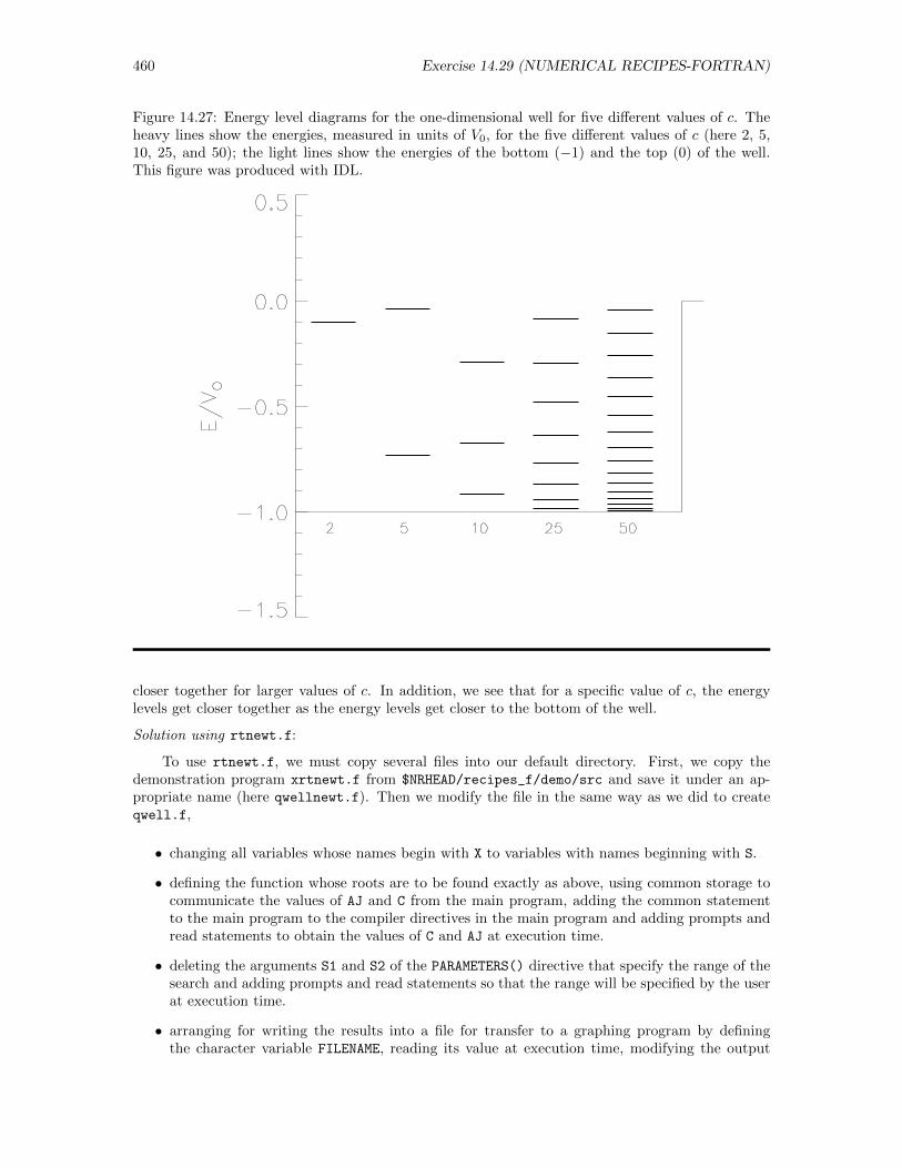
460 Exercise 14.29 (NUMERICAL RECIPES-FORTRAN)
Figure 14.27: Energy level diagrams for the one-dimensional well for five different values of c. Theheavy lines show the energies, measured in units of V0, for the five different values of c (here 2, 5,10, 25, and 50); the light lines show the energies of the bottom (−1) and the top (0) of the well.This figure was produced with IDL.
closer together for larger values of c. In addition, we see that for a specific value of c, the energylevels get closer together as the energy levels get closer to the bottom of the well.
Solution using rtnewt.f:
To use rtnewt.f, we must copy several files into our default directory. First, we copy thedemonstration program xrtnewt.f from $NRHEAD/recipes_f/demo/src and save it under an ap-propriate name (here qwellnewt.f). Then we modify the file in the same way as we did to createqwell.f,
• changing all variables whose names begin with X to variables with names beginning with S.
• defining the function whose roots are to be found exactly as above, using common storage tocommunicate the values of AJ and C from the main program, adding the common statementto the main program to the compiler directives in the main program and adding prompts andread statements to obtain the values of C and AJ at execution time.
• deleting the arguments S1 and S2 of the PARAMETERS() directive that specify the range of thesearch and adding prompts and read statements so that the range will be specified by the userat execution time.
• arranging for writing the results into a file for transfer to a graphing program by definingthe character variable FILENAME, reading its value at execution time, modifying the output
Exercise 14.29 (NUMERICAL RECIPES-FORTRAN) 461
statement to write to this file rather than to the screen and,after all output has been produced,closing the file.
• defining the function to return a derivative by adding the external function FUNCD defined by
SUBROUTINE FUNCD(S,FN,DF)
COMMON /INPUTVARS/ AJ, C
FN=SIN(S) + AJ*S/C
DF=COS(S) + AJ/C
RETURN
These provisions allow the user to run the program multiple times without having to recompile it.The resulting program is
PROGRAM QWELLNEWT
EXTERNAL FUNCD, FUNC
CHARACTER*20 FILENAME
PARAMETER(N=100,NBMAX=20)
DIMENSION SB1(NBMAX),SB2(NBMAX)
COMMON /INPUTVARS/ AJ, C
NB=NBMAX
WRITE(*, ’(1X,A)’) ’Enter a value for c = ’
READ(*, *) C
WRITE(*, ’(1X,A)’) ’Enter a value for the lower bound = ’
READ(*, *) S1
WRITE(*, ’(1X,A)’) ’Enter a value for the upper bound = ’
READ(*, *) S2
WRITE(*, *) ’Enter -1 for an upper solution and 1 for a lower’
WRITE(*, *) ’solution =’
READ(*, *) J
WRITE(*, *) ’Enter an appropriate file name(ends in .dat’
WRITE(*, *) ’and is less than 20 characters):’
READ(*, FMT=’(A)’) FILENAME
CALL ZBRAK(FUNC,S1,S2,N,SB1,SB2,NB)
OPEN(UNIT=1, FILE = NAME, STATUS = ’NEW’)
DO I=1,NB
SACC=(1.0E-6)
ROOT=RTNEWT(FUNCD,SB1(I),SB2(I),SACC)
WRITE(1,’(F12.6)’) ROOT
ENDDO
CLOSE( UNIT=1)
END
FUNCTION FUNC(S)
COMMON /INPUTVARS/ AJ, C
FUNC = SIN(S) + AJ*S/C
END
SUBROUTINE FUNCD(S,FN,DF)
COMMON /INPUTVARS/ J, C
FN=SIN(S) + J*S/C
DF=COS(S) + J/C
RETURN
END

462 Exercise 14.29 (NUMERICAL RECIPES-FORTRAN)
Finally, we must copy the files rtnewt.f and, if it is not still there, zbrak.f from$NRHEAD/recipes_f/recipes into our default directory and compile qwellnewt.f (along withrtbis.f and zbrak.f) with the statement
f77 -o qwellnewt.xf qwell.f rtbis.f zbrak.f
This program can then be run in the same way—and with the same input—as qwell.xf. Wesuppress output because it is the same as the output already described for the first program.
Exercise 14.14 (NUMERICAL RECIPES-C) 463
14.14 Natural Frequencies of Bar (NUMERICAL RECIPES-C)
Exercise: The natural frequencies for the transverse vibrations of a bar of uniform cross sectionthat has length L and is free at both ends are given by
ωn =4K
L2
√E
ρα2n
where K is the radius of gyration of the cross section of the bar, E is Young’s modulus for thematerial of the bar, ρ is the density (mass/unit volume) of the material of the bar, and αn is asolution to the equation
tanα = ± tanhα
Find the lowest half dozen natural frequencies for this bar. [A detailed discussion of this exercise canbe found in N. H. Fletcher and T. D. Rossing, The Physics of Musical Instruments, Second Edition(Springer-Verlag, New York, 1991), pp. 57ff.]
Solution: The natural frequencies for the transverse vibrations of a bar of uniform cross sectionare given by the equation
ωn =4K
L2
√E
ρα2n
where L is the length of the bar, K is the radius of gyration of the cross-section of the bar, E isYoung’s modulus for the material of the bar, ρ is the density of the material of the bar, and αn is asolution to the equation
tan(α) = ± tanh(α)
Since K,L,E, and ρ are fixed for a given bar, the relationships among the natural frequencies ofthat bar are determined by αn. The previous equation can be rewritten as
tan(α)∓ tanh(α) = 0
Therefore, we can find the first six values of α2n, and thus the lowest half dozen natural frequencies
of the bar, by finding the roots of this equation and then squaring them.
As a start, we must have some idea where the roots we seek lie. Thus, graphs of the functionsy = tan(α) − tanh(α) and y = tan(α) + tanh(α) should be made. A graph of these functions ispresented in Fig. 14.28.12 From this graph we conclude that the first six roots lie in the intervals
tan(α) = − tanh(α) 2.0 < x < 3.0 5.2 < x < 6.0 8.0 < x < 9.0tan(α) = tanh(α) 3.5 < x < 4.5 6.5 < x < 7.5 10.0 < x < 10.7
You should use a program with which you are familiar to generate this—or an equivalent—graph.Note in particular that the divergences of the tangent function (1) complicate the production ofa graph that does not have extraneous and erroneous (nearly) vertical lines at α equal to an oddmultiple of π/2 and (2) make it critical to avoid embracing any of these special values of α in anyof the intervals in which we seek a root.
To find the roots of this equation, we choose first to use the Numerical Recipe rtbis.c, whichwe must copy to the default directory from the directory $NRHEAD/recipes_c-ansi/recipes. Asa start on a suitable driving program, we also copy the demonstration program xrtbis.c from$NRHEAD/recipes_c-ansi/demo/src, saving it under the name natfreq bisect.c. Then, we mod-ify the demonstration program in the following ways:
12C by itself does not offer the possibility of making such graphs. The graph shown was produced by IDL. Thecoding used to create an equivalent graph in the program(s) incorporated in this document is recorded at the end ofthis solution.
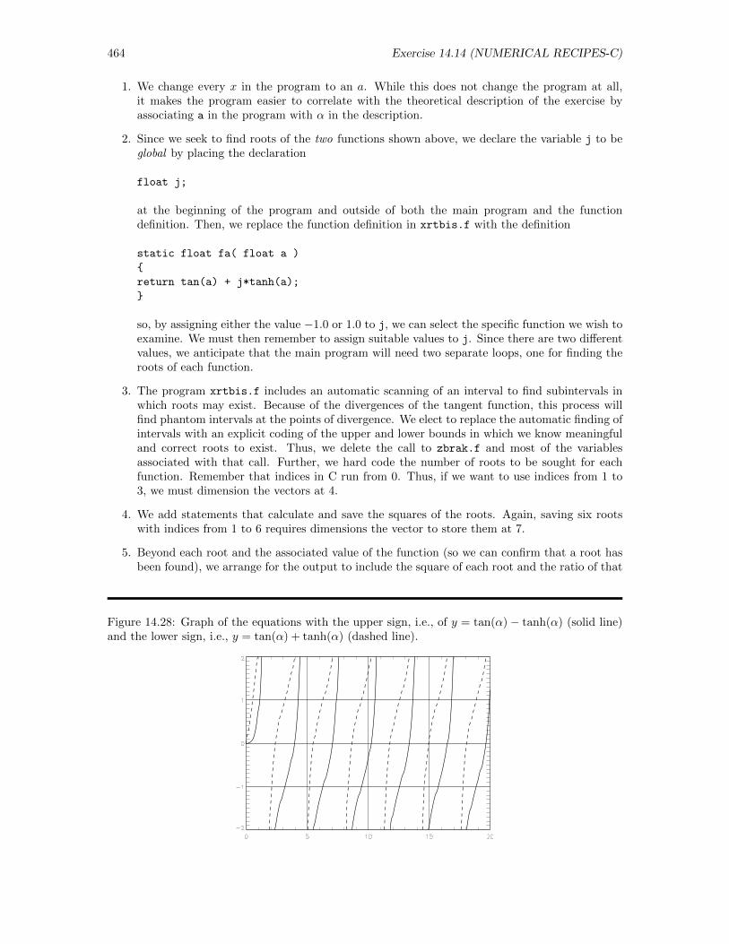
464 Exercise 14.14 (NUMERICAL RECIPES-C)
1. We change every x in the program to an a. While this does not change the program at all,it makes the program easier to correlate with the theoretical description of the exercise byassociating a in the program with α in the description.
2. Since we seek to find roots of the two functions shown above, we declare the variable j to beglobal by placing the declaration
float j;
at the beginning of the program and outside of both the main program and the functiondefinition. Then, we replace the function definition in xrtbis.f with the definition
static float fa( float a )
return tan(a) + j*tanh(a);
so, by assigning either the value −1.0 or 1.0 to j, we can select the specific function we wish toexamine. We must then remember to assign suitable values to j. Since there are two differentvalues, we anticipate that the main program will need two separate loops, one for finding theroots of each function.
3. The program xrtbis.f includes an automatic scanning of an interval to find subintervals inwhich roots may exist. Because of the divergences of the tangent function, this process willfind phantom intervals at the points of divergence. We elect to replace the automatic finding ofintervals with an explicit coding of the upper and lower bounds in which we know meaningfuland correct roots to exist. Thus, we delete the call to zbrak.f and most of the variablesassociated with that call. Further, we hard code the number of roots to be sought for eachfunction. Remember that indices in C run from 0. Thus, if we want to use indices from 1 to3, we must dimension the vectors at 4.
4. We add statements that calculate and save the squares of the roots. Again, saving six rootswith indices from 1 to 6 requires dimensions the vector to store them at 7.
5. Beyond each root and the associated value of the function (so we can confirm that a root hasbeen found), we arrange for the output to include the square of each root and the ratio of that
Figure 14.28: Graph of the equations with the upper sign, i.e., of y = tan(α)− tanh(α) (solid line)and the lower sign, i.e., y = tan(α) + tanh(α) (dashed line).
Exercise 14.14 (NUMERICAL RECIPES-C) 465
square to the square of the lowest root (so we can easily compare the natural frequencies withone another).
6. We change all comments to fit our program.
With these changes, our final program natfreq bisect.c is
/* Program natfreq_bisect.c */
#include <stdio.h>
#include <math.h>
#include "nr.h"
#include "nrutil.h"
float j; /* Set j global */
static float fa( float a ) /* Define function */
return tan(a) + j*tanh(a);
int main(void)
int i; /* Loop index */
float aacc, root, tmp;
float ab1[4], ab2[4], sqr[7]; /* Bounds, square of root */
aacc = 1.0e-6; /* Set precision */
j = 1.0; /* Set for tan(a)+tanh(a) */
ab1[1] = 2.0; ab2[1] = 3.0; /* Set bounds */
ab1[2] = 5.2; ab2[2] = 6.0;
ab1[3] = 8.0; ab2[3] = 9.0;
printf("\n The roots of tan(a) + tanh(a) their squares:\n" );
printf("\n%21s %15s %13s %15s\n\n","a","f(a)","a^2", "a^2/a1^2");
for (i=1;i<=3;i++) /* Find, save display roots */
root = rtbis( fa, ab1[i], ab2[i], aacc );
sqr[2*i-1] = pow( root, 2 );
tmp = sqr[2*i-1]/sqr[1];
printf("root %3d %14.6f %14.6f %14.6f %14.6f\n",
2*i-1, root, fa(root), sqr[2*i-1], tmp );
j = -1; /* Set for tan(a)-tanh(a) */
ab1[1] = 3.5; ab2[1] = 4.5; /* Set bounds */
ab1[2] = 6.5; ab2[2] = 7.5;
ab1[3] = 10.0; ab2[3] = 10.7;
printf("\n The roots of tan(a) - tanh(a) and their squares:\n" );
printf("\n%21s %15s %13s %15s\n\n","a","f(a)","a^2", "a^2/a1^2");
for (i=1;i<=3;i++) /* Find, save, display roots */
root = rtbis( fa, ab1[i], ab2[i], aacc );
466 Exercise 14.14 (NUMERICAL RECIPES-C)
sqr[2*i] = pow( root, 2 );
tmp = sqr[2*i]/sqr[1];
printf("root %3d %14.6f %14.6f %14.6f %14.6f\n",
2*i, root, fa(root), sqr[2*i], tmp );
return 0;
Next, we must copy the files nr.h and nrutil.h from $NRHEAD/recipes_c-ansi/include andnrutil.c from $NRHEAD/recipes_c-ansi/recipes into our default directory. We now compile andlink natfreq bisect.c, rtbis.c, and nrutil.c with the statement
cc -o natfreq_bisect.xc natfreq.c nrutil.c rtbis.c -lm
and then run the program with the statement
./natfreq_bisect.xc
The resulting output is
The roots of tan(a) + tanh(a) and their squares:
a f(a) a^2 a^2/a1^2
root 1 2.365020 -0.000001 5.593318 1.000000
root 3 5.497804 0.000000 30.225845 5.403920
root 5 8.639380 -0.000001 74.638878 13.344293
The roots of tan(a) - tanh(a) and their squares:
a f(a) a^2 a^2/a1^2
root 2 3.926601 -0.000002 15.418199 2.756539
root 4 7.068583 0.000000 49.964859 8.932955
root 6 10.210176 -0.000001 104.247681 18.637896
We conclude that the values of α2n that correspond to the lowest six natural frequencies are 5.593318,
15.418199, 30.225845, 49.964859, 74.638878, and 104.247681, though not all the digits reported aresignificant. Thus, we determine that the natural frequencies themselves are given by
ω1 = 5.5933184K
L2
√E
ρω2 = 15.418199
4K
L2
√E
ρ= 2.756539ω1
ω3 = 30.2258454K
L2
√E
ρ= 5.403920ω1 ω4 = 49.964859
4K
L2
√E
ρ= 8.932955ω1
ω5 = 74.6388784K
L2
√E
ρ= 13.344293ω1 ω6 = 104.247681
4K
L2
√E
ρ= 18.637896ω1
Similar edits to the demo program xrtnewt.c, though adding the procedure funcd that returnsboth the function and its first derivative, produces the program natfreq newt.f:
Exercise 14.14 (NUMERICAL RECIPES-C) 467
/* Program natfreq_newt.c */
#include <stdio.h>
#include <math.h>
#include "nr.h"
#include "nrutil.h"
float j; /* Set j global */
static float fa(float a)
return tan(a) + j*tanh(a);
static void funcd(float a,float *fn, float *df)
*fn = tan(a) + j*tanh(a);
*df = pow( tan(a), 2 ) - j * pow( tanh(a), 2 ) + j + 1.0;
int main(void)
int i; /* Loop index */
float aacc, root, tmp;
float ab1[4], ab2[4], sqr[7]; /* Bounds, square of root */
j = 1.0; /* Set for tan(a)+tanh(a) */
ab1[1] = 2.0; ab2[1] = 3.0; /* Set bounds */
ab1[2] = 5.2; ab2[2] = 6.0;
ab1[3] = 8.0; ab2[3] = 9.0;
printf("\n The roots of tan(a) + tanh(a) and their squares:\n" );
printf("\n%21s %15s %13s %15s\n\n","a","f(a)","a^2", "a^2/a1^2");
for (i=1;i<=3;i++) /* Find, save display roots */
aacc = (1.0e-6)*(ab1[i]+ab2[i])/2.0;
root = rtnewt( funcd, ab1[i], ab2[i], aacc );
sqr[2*i-1] = pow( root, 2 );
tmp = sqr[2*i-1]/sqr[1];
printf("root %3d %14.6f %14.6f %14.6f %14.6f\n",
2*i-1, root, fa(root), sqr[2*i-1], tmp );
j = -1; /* Set for tan(a)-tanh(a) */
ab1[1] = 3.5; ab2[1] = 4.5; /* Set bounds */
ab1[2] = 6.5; ab2[2] = 7.5;
ab1[3] = 10.0; ab2[3] = 10.7;
printf("\n The roots of tan(a) - tanh(a) and their squares:\n" );
printf("\n%21s %15s %13s %15s\n\n","a","f(a)","a^2", "a^2/a1^2");
for (i=1;i<=3;i++) /* Find, save display roots */
aacc = (1.0e-6)*(ab1[i]+ab2[i])/2.0;
root = rtnewt( funcd, ab1[i], ab2[i], aacc );
468 Exercise 14.14 (NUMERICAL RECIPES-C)
sqr[2*i] = pow( root, 2 );
tmp = sqr[2*i]/sqr[1];
printf("root %3d %14.6f %14.6f %14.6f %14.6f\n",
2*i, root, fa(root), sqr[2*i], tmp );
return 0;
This program uses the alternative recipe rtnewt.c and can be compiled, linked, and run with thestatements
cc -o natfreq_newt.xc natfreq_newt.c rtnewt.c nrutil.c -lm
./natfreq_newt.xc
The resulting output is
The roots of tan(a) + tanh(a) and their squares:
a f(a) a^2 a^2/a1^2
root 1 2.365020 0.000000 5.593321 1.000000
root 3 5.497804 0.000000 30.225845 5.403918
root 5 8.639380 -0.000001 74.638878 13.344287
The roots of tan(a) - tanh(a) and their squares:
a f(a) a^2 a^2/a1^2
root 2 3.926602 0.000000 15.418206 2.756539
root 4 7.068583 0.000000 49.964859 8.932951
root 6 10.210176 0.000001 104.247704 18.637892
Within roundoff error, this output is entirely consistent with that produced by the first program.
IDL Code
; Establish independent and dependent variables
alpha = findgen(401)/20.0 ; 0.0 <= alpha <= 20.0, 0.05 increment
; 401 entries
y1 = tan(alpha) + tanh(alpha)
y2 = tan(alpha) - tanh(alpha)
; Determine indices at which functions diverge. They
; are the same for both y1 and y2.
for i = 0, 399 do $
if signum(y1[i]) eq 1 and signum(y1[i+1])eq -1 then print, i
; 31 94 157 219 282 345
ind = [ 31, 94, 157, 219, 282, 345, 402] ; Add 400+2 to final segment of graph
; Plot y1 and y2, avoiding the points of divergence by 2 entries
plot, alpha[0:30],y1[0:30], ticklen=1, linestyle=2, thick=3, $
xrange=[0.0,20.0], yrange=[-2.0,2.0]
oplot, alpha[0:30],y2[0:30], thick=3
for i = 0,5 do begin $

Exercise 14.14 (NUMERICAL RECIPES-C) 469
st=ind[i]+2 & en=ind[i+1]-2 & $
oplot, alpha[st:en],y1[st:en], linestyle=2, thick=3 & $
oplot, alpha[st:en],y2[st:en], thick=3 & $
end
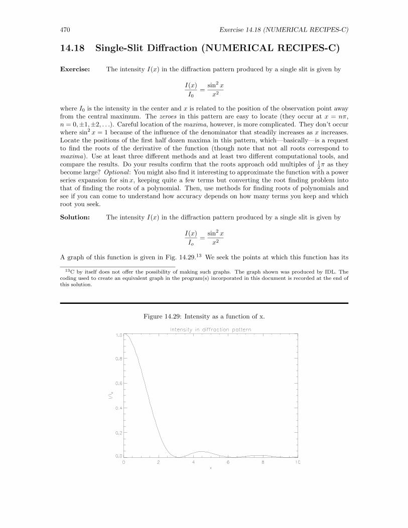
470 Exercise 14.18 (NUMERICAL RECIPES-C)
14.18 Single-Slit Diffraction (NUMERICAL RECIPES-C)
Exercise: The intensity I(x) in the diffraction pattern produced by a single slit is given by
I(x)
I0=
sin2 x
x2
where I0 is the intensity in the center and x is related to the position of the observation point awayfrom the central maximum. The zeroes in this pattern are easy to locate (they occur at x = nπ,n = 0,±1,±2, . . .). Careful location of the maxima, however, is more complicated. They don’t occurwhere sin2 x = 1 because of the influence of the denominator that steadily increases as x increases.Locate the positions of the first half dozen maxima in this pattern, which—basically—is a requestto find the roots of the derivative of the function (though note that not all roots correspond tomaxima). Use at least three different methods and at least two different computational tools, andcompare the results. Do your results confirm that the roots approach odd multiples of 1
2π as theybecome large? Optional : You might also find it interesting to approximate the function with a powerseries expansion for sinx, keeping quite a few terms but converting the root finding problem intothat of finding the roots of a polynomial. Then, use methods for finding roots of polynomials andsee if you can come to understand how accuracy depends on how many terms you keep and whichroot you seek.
Solution: The intensity I(x) in the diffraction pattern produced by a single slit is given by
I(x)
Io=
sin2 x
x2
A graph of this function is given in Fig. 14.29.13 We seek the points at which this function has its
13C by itself does not offer the possibility of making such graphs. The graph shown was produced by IDL. Thecoding used to create an equivalent graph in the program(s) incorporated in this document is recorded at the end ofthis solution.
Figure 14.29: Intensity as a function of x.
Exercise 14.18 (NUMERICAL RECIPES-C) 471
maxima, i.e., the points at which
g(x) =d
dx
(sin2 x
x2
)=
2 sinx cosx
x2− 2 sin2 x
x3= 0
Using the C version of Numerical Recipes routines to locate the roots of this equation is quite simple.Furthermore, we see from the graph that the maxima occur at every other root of the first derivative.
We can use two different methods to find the roots of the first derivative of the intensityfunction. To use rtbis.c, we copy xrtbis.c from $NRHEAD/recipes_c-ansi/demo/src into thedefault directory under a new name (here ex18bin.c). It appears from the graph that if we modifyour parameters to take us through the range −0.5 ≤ x ≤ 20.0 or so, we will be able to find the firstsix maxima. We must also tell the program that we are using an external function fx, which wedefine in the beginning to be the first derivative of our intensity function. Furthermore, we add thestatement #include <math.h> so that we can use the sine, cosine, and pow functions. Finally, wemodify the xacc parameter in the for loop to be just 1.0e− 6. The resulting program is
/* ex18bin.c */
#include <stdio.h>
#include <math.h>
#include "nr.h"
#include "nrutil.h"
#define N 150
#define NBMAX 20
#define X1 -0.5
#define X2 20.0
static float fx(float x)
return 2*sin(x)*cos(x)*pow(x, -2.0) - 2.0*pow(x, -3.0)*pow(sin(x), 2.0);
int main(void)
int i, nb=NBMAX;
float xacc, root, xb1[NBMAX+1], xb2[NBMAX+1];
zbrak( fx, X1, X2, N, xb1, xb2, &nb );
printf("%21s %15s\n","x","f(x)");
for ( i=1; i<=nb; i++ )
xacc = 1.0e-6;
root = rtbis( fx, xb1[i], xb2[i], xacc );
printf( "root %3d %14.6f %14.4e\n", i, root, fx(root) );
This program prints the roots in the designated range. It also determines the value of thefunction at the point, so we can see how close it actually is to 0. After copying rtbis.c,zbrak.c, and nrutil.c from $NRHEAD/recipes_c-ansi/recipes and nr.h and nrutil.h from$NRHEAD/recipes_c-ansi/include, we can compile, link, and execute the program by invoking thestatements
cc -o ex18bin.xc ex18bin.c rtbis.c zbrak.c nrutil.c -lm
./ex18bin.xc
472 Exercise 14.18 (NUMERICAL RECIPES-C)
The resulting output is
x f(x)
root 1 0.000000 -2.0210e-07
root 2 3.141593 -3.0598e-08
root 3 4.493410 -1.6585e-08
root 4 6.283185 -1.5299e-08
root 5 7.725252 -1.0368e-08
root 6 9.424777 -2.0936e-08
root 7 10.904122 -1.1563e-08
root 8 12.566370 -7.6495e-09
root 9 14.066195 -6.2504e-09
root 10 15.707963 -2.2545e-09
root 11 17.220757 -8.4612e-09
root 12 18.849554 -1.0468e-08
By comparing our results to the graph, we can see that the first root corresponds to a maximum,the second to a minimum and so forth. Thus, the maxima are roots 1, 3, 5, etc.
To use rtnewt.c, we follow essentially the same procedure. Assuming that we already havenr.h, nrutil.h, zbrak.c, and nrutil.c in our default directory, we only have to copy two morefiles into our defualt directory. We must copy xrtnewt.c from $NRHEAD/recipes_c-ansi/demo/src
(saving it under the name ex18newt.c) and rtnewt.c from $NRHEAD/recipes_c-ansi/recipes. Wemodify rtnewt.c in much the same way we did rtbis.c, only we also have to find the derivativeof the function whose roots we wish to locate, the second derivative of the intensity equation. Themodified program is
/* Program ex18newt.c */
#include <stdio.h>
#include <math.h>
#include "nr.h"
#include "nrutil.h"
#define N 150
#define NBMAX 20
#define X1 -0.5
#define X2 20.0
static float fx(float x)
return 2*sin(x)*cos(x)*pow(x, -2.0) - 2.0*pow(x, -3.0)*pow(sin(x), 2.0);
static void funcd(float x,float *fn, float *df)
*fn= 2.0*cos(x)*sin(x)*pow(x, -2.0) - 2.0*pow(sin(x), 2.0)*pow(x,-3.0);
*df = 2*pow(x, -2.0)*(pow(cos(x), 2.0)-pow(sin(x), 2.0)-
2*sin(x)*cos(x)/x) - 4*sin(x)*cos(x)*pow(x, -3.0)+
6*pow(sin(x),2.0)*pow(x, -4.0);
int main(void)
int i, nb=NBMAX;
Exercise 14.18 (NUMERICAL RECIPES-C) 473
float xacc,root, xb1[NBMAX+1], xb2[NBMAX+1];
zbrak( fx, X1, X2, N, xb1, xb2, &nb );
printf("%21s %15s\n","x","f(x)");
for (i=1;i<=nb;i++)
xacc=(1.0e-6);
root=rtnewt(funcd,xb1[i],xb2[i],xacc);
printf("root %3d %14.6f %14.4e\n",i,root,fx(root));
When the program is compiled and executed with the statements
cc -o ex18newt.xc ex18newt.c zbrak.c nrutil.c rtnewt.c -lm
./ex18newt.xc
the screen displays the results
x f(x)
root 1 0.000000 3.8147e-06
root 2 3.141593 1.7716e-08
root 3 4.493410 -1.6585e-08
root 4 6.283185 8.8578e-09
root 5 7.725252 5.3489e-09
root 6 9.424778 5.3700e-10
root 7 10.904121 4.3453e-09
root 8 12.566371 4.4289e-09
root 9 14.066194 3.3411e-09
root 10 15.707963 -2.2545e-09
root 11 17.220755 4.3590e-09
root 12 18.849556 2.6850e-10
for the roots. A comparison to the graph shows us just as before that the odd numbered rootscorrespond to the maxima. Notice that the roots found by rtbis.c are very similar to those foundby rtnewt.c.
IDL Code
x=findgen(101)/10.0
i=(sin(x))^2/x^2.0
i[0] = 1.0
plot, x, i, title=’Intensity in diffraction pattern’, $
xtitle=’x’, ytitle=’I/I!Do!N’
474 Exercise 14.19 (NUMERICAL RECIPES-C)
14.19 Roots of J0(x) (NUMERICAL RECIPES-C)
Exercise: Using at least three different methods and at least two different computationaltools, find the first half dozen roots of the zeroth-order Bessel function J0(x). Note that theseroots are related to the radii of circular nodes in some of the vibrations of a circular membrane.The values of these roots tabulated in Abramowitz and Stegun14 are 2.4048255577, 5.5200781103,8.6537279129, 11.7915344391, 14.9309177086, 18.0710639679. Hint : Most computational tools havebuilt-in capabilities for evaluating the Bessel functions. Consult the appropriate vendor manuals.
Solution: We wish to know the first half dozen roots of the zeroth-order Bessel function.The values of the roots as tabulated by Abramowitz and Stegun are 2.40485 55577, 5.52007 81103,8.65372 79129, 11.79153 44391, 14.93091 77086, and 18.07106 39679. Using rtbis.c in C, we canevaluate the Bessel function quickly by noticing that there are recipes for different orders of the func-tion. We can copy the xrtbis.c driver from $NRHEAD/recipes_c-ansi/demo/src into our defaultdirectory (saving it as bessrtbis.c). In addition, we copy the files rtbis.c, zbrak.c, nrutil.c,and bessj0.c from $NRHEAD/recipes_c-ansi/recipes into our default directory. Finally, we mustcopy nr.h and nrutil.h from $NRHEAD/recipes_c-ansi/include into our default directory. Whenwe open bessrtbis.c to modify it, we see that the function we want is already in place to be eval-uated. It will, however, use 20 iterations to find all the roots in the range 1.0 ≤ x ≤ 50.0. If we donot mind the extra roots, we can simply execute the program by entering the statements
cc -o bessrtbis.xc bessrtbis.c zbrak.c bessj0.c nrutil.c rtbis.c -lm
./bessrtbis.xc
The roots found are as follows.
Roots of bessj0:
x f(x)
root 1 2.404827 -0.000001
root 2 5.520077 0.000000
root 3 8.653729 0.000000
root 4 11.791533 0.000000
root 5 14.930930 -0.000003
root 6 18.071054 -0.000002
root 7 21.211639 0.000000
root 8 24.352465 -0.000001
root 9 27.493486 -0.000001
root 10 30.634581 -0.000004
root 11 33.775833 -0.000002
root 12 36.917088 -0.000001
root 13 40.058434 -0.000001
root 14 43.199783 -0.000001
root 15 46.341213 -0.000003
root 16 49.482594 -0.000002
To use rtnewt, we follow essentially the same procedure. Assuming that we alreadyhave nr.h, nrutil.h, zbrak.c, nrutil.c, and bessj0.c in our default directory, we onlyhave to copy three more files into our default directory. We must copy xrtnewt.c from$NRHEAD/recipes_c-ansi/demo/src (saving it under the name bessrtnewt.c) and rtnewt.c andbessj1.c from $NRHEAD/recipes_c-ansi/recipes. Now, we need only compile and run the pro-gram since the Bessel function is again the demo function. We compile and run the program withthe statements
14M. Abramowitz and I. A. Stegun, Handbook of Mathematical Functions, U. S. Department of Commerce, AppliedMathematics Series #55, 1964.
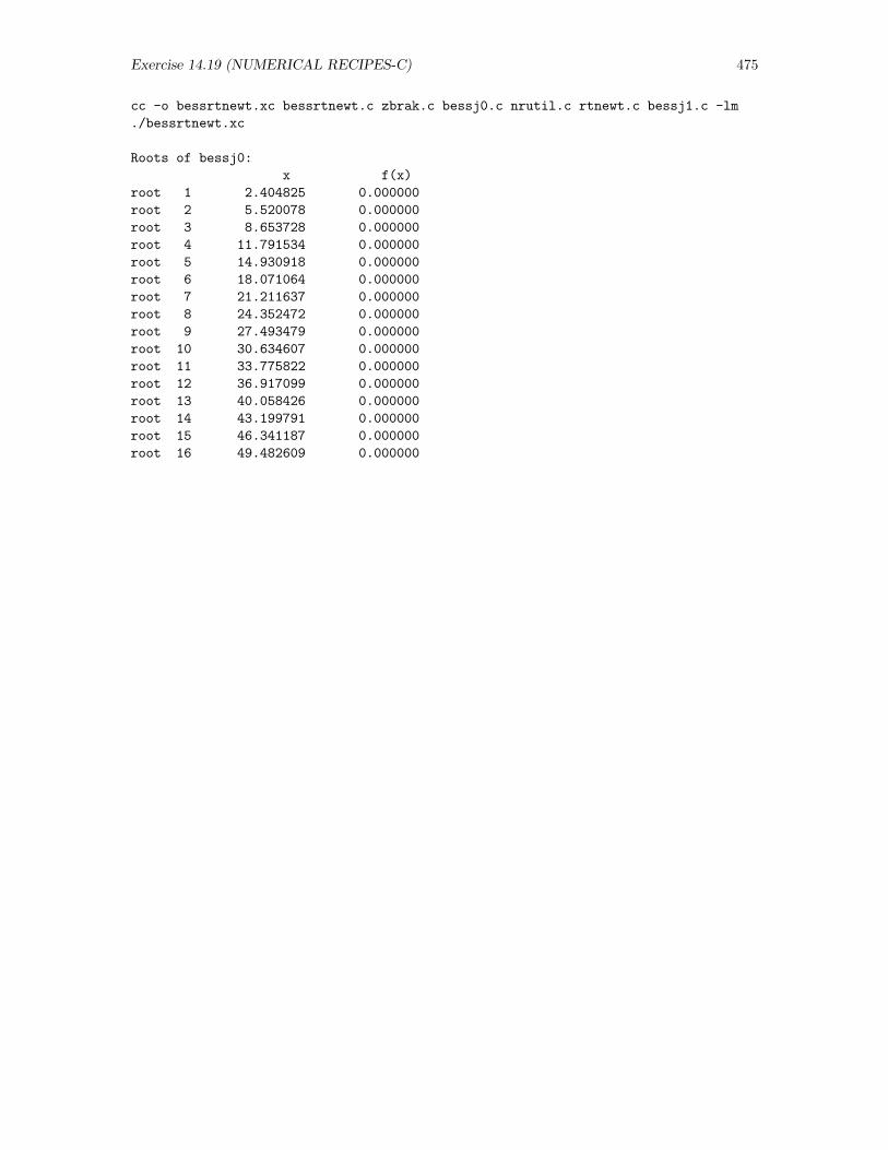
Exercise 14.19 (NUMERICAL RECIPES-C) 475
cc -o bessrtnewt.xc bessrtnewt.c zbrak.c bessj0.c nrutil.c rtnewt.c bessj1.c -lm
./bessrtnewt.xc
Roots of bessj0:
x f(x)
root 1 2.404825 0.000000
root 2 5.520078 0.000000
root 3 8.653728 0.000000
root 4 11.791534 0.000000
root 5 14.930918 0.000000
root 6 18.071064 0.000000
root 7 21.211637 0.000000
root 8 24.352472 0.000000
root 9 27.493479 0.000000
root 10 30.634607 0.000000
root 11 33.775822 0.000000
root 12 36.917099 0.000000
root 13 40.058426 0.000000
root 14 43.199791 0.000000
root 15 46.341187 0.000000
root 16 49.482609 0.000000
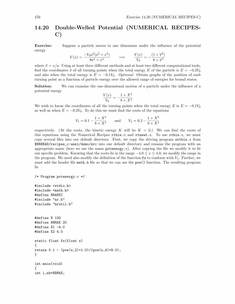
476 Exercise 14.20 (NUMERICAL RECIPES-C)
14.20 Double-Welled Potential (NUMERICAL RECIPES-C)
Exercise: Suppose a particle moves in one dimension under the influence of the potentialenergy
V (x) =−V0a
2(a2 + x2)
8a4 + x4=⇒ V (x)
V0= − (1 + x2)
8 + x4
where x = x/a. Using at least three different methods and at least two different computational tools,find the coordinates x of all turning points when the total energy E of the particle is E = −0.2V0
and also when the total energy is E = −0.1V0. Optional : Obtain graphs of the position of eachturning point as a function of particle energy over the allowed range of energies for bound states.
Solution: We can examine the one-dimensional motion of a particle under the influence of apotential energy
V (x)
V0= −1 +X2
8 +X4
We wish to know the coordinates of all the turning points when the total energy E is E = −0.1V0
as well as when E = −0.2V0. To do this we must find the roots of the equations
V1 = 0.1− 1 +X2
8 +X4and V2 = 0.2− 1 +X2
8 +X4
respectively. (At the roots, the kinetic energy K will be K = 0.) We can find the roots ofthis equations using the Numerical Recipes rtbis.c and rtnewt.c. To use rtbis.c, we mustcopy several files into our default directory. First, we copy the driving program xrtbis.c from$NRHEAD/recipes_c-ansi/demo/src into our default directory and rename the program with anappropriate name (here we use the name potenergy.c). After copying the file we modify it to fitour specific problem. Knowing that the roots lie in the range −4.0 ≤ x ≤ 4.0, we modify the range inthe program. We need also modify the definition of the function fx to conform with V1. Further, wemust add the header file math.h file so that we can use the pow() function. The resulting programlis
/* Program potenergy.c */
#include <stdio.h>
#include <math.h>
#define NRANSI
#include "nr.h"
#include "nrutil.h"
#define N 100
#define NBMAX 20
#define X1 -4.0
#define X2 4.0
static float fx(float x)
return 0.1 - (pow(x,2)+1.0)/(pow(x,4)+8.0);
int main(void)
int i,nb=NBMAX;
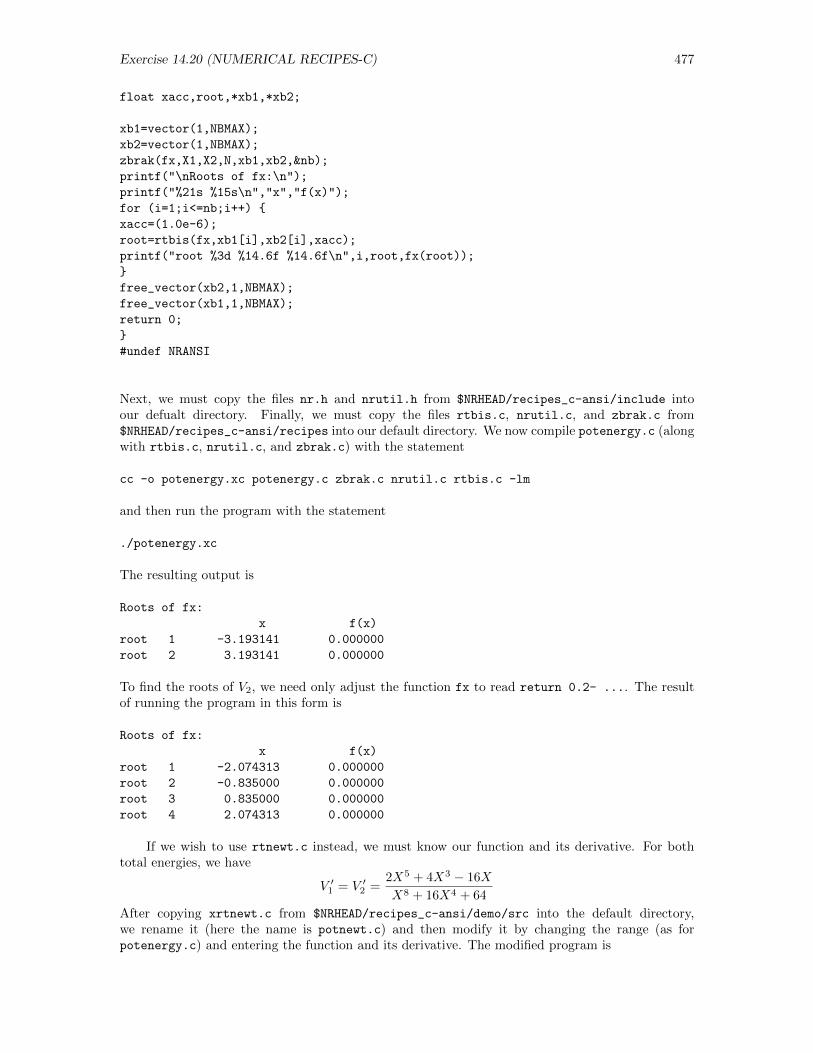
Exercise 14.20 (NUMERICAL RECIPES-C) 477
float xacc,root,*xb1,*xb2;
xb1=vector(1,NBMAX);
xb2=vector(1,NBMAX);
zbrak(fx,X1,X2,N,xb1,xb2,&nb);
printf("\nRoots of fx:\n");
printf("%21s %15s\n","x","f(x)");
for (i=1;i<=nb;i++)
xacc=(1.0e-6);
root=rtbis(fx,xb1[i],xb2[i],xacc);
printf("root %3d %14.6f %14.6f\n",i,root,fx(root));
free_vector(xb2,1,NBMAX);
free_vector(xb1,1,NBMAX);
return 0;
#undef NRANSI
Next, we must copy the files nr.h and nrutil.h from $NRHEAD/recipes_c-ansi/include intoour defualt directory. Finally, we must copy the files rtbis.c, nrutil.c, and zbrak.c from$NRHEAD/recipes_c-ansi/recipes into our default directory. We now compile potenergy.c (alongwith rtbis.c, nrutil.c, and zbrak.c) with the statement
cc -o potenergy.xc potenergy.c zbrak.c nrutil.c rtbis.c -lm
and then run the program with the statement
./potenergy.xc
The resulting output is
Roots of fx:
x f(x)
root 1 -3.193141 0.000000
root 2 3.193141 0.000000
To find the roots of V2, we need only adjust the function fx to read return 0.2- .... The resultof running the program in this form is
Roots of fx:
x f(x)
root 1 -2.074313 0.000000
root 2 -0.835000 0.000000
root 3 0.835000 0.000000
root 4 2.074313 0.000000
If we wish to use rtnewt.c instead, we must know our function and its derivative. For bothtotal energies, we have
V ′1 = V ′2 =2X5 + 4X3 − 16X
X8 + 16X4 + 64
After copying xrtnewt.c from $NRHEAD/recipes_c-ansi/demo/src into the default directory,we rename it (here the name is potnewt.c) and then modify it by changing the range (as forpotenergy.c) and entering the function and its derivative. The modified program is
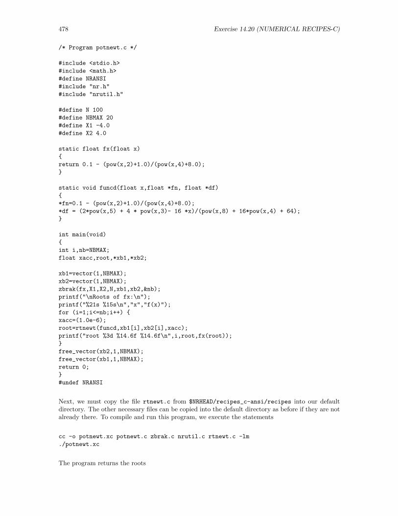
478 Exercise 14.20 (NUMERICAL RECIPES-C)
/* Program potnewt.c */
#include <stdio.h>
#include <math.h>
#define NRANSI
#include "nr.h"
#include "nrutil.h"
#define N 100
#define NBMAX 20
#define X1 -4.0
#define X2 4.0
static float fx(float x)
return 0.1 - (pow(x,2)+1.0)/(pow(x,4)+8.0);
static void funcd(float x,float *fn, float *df)
*fn=0.1 - (pow(x,2)+1.0)/(pow(x,4)+8.0);
*df = (2*pow(x,5) + 4 * pow(x,3)- 16 *x)/(pow(x,8) + 16*pow(x,4) + 64);
int main(void)
int i,nb=NBMAX;
float xacc,root,*xb1,*xb2;
xb1=vector(1,NBMAX);
xb2=vector(1,NBMAX);
zbrak(fx,X1,X2,N,xb1,xb2,&nb);
printf("\nRoots of fx:\n");
printf("%21s %15s\n","x","f(x)");
for (i=1;i<=nb;i++)
xacc=(1.0e-6);
root=rtnewt(funcd,xb1[i],xb2[i],xacc);
printf("root %3d %14.6f %14.6f\n",i,root,fx(root));
free_vector(xb2,1,NBMAX);
free_vector(xb1,1,NBMAX);
return 0;
#undef NRANSI
Next, we must copy the file rtnewt.c from $NRHEAD/recipes_c-ansi/recipes into our defaultdirectory. The other necessary files can be copied into the default directory as before if they are notalready there. To compile and run this program, we execute the statements
cc -o potnewt.xc potnewt.c zbrak.c nrutil.c rtnewt.c -lm
./potnewt.xc
The program returns the roots
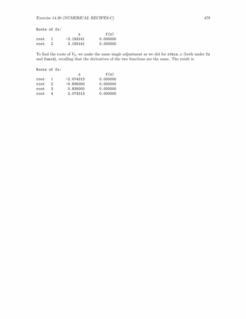
Exercise 14.20 (NUMERICAL RECIPES-C) 479
Roots of fx:
x f(x)
root 1 -3.193141 0.000000
root 2 3.193141 0.000000
To find the roots of V2, we make the same single adjustment as we did for rtbis.c (both under fxand funcd), recalling that the derivatives of the two functions are the same. The result is
Roots of fx:
x f(x)
root 1 -2.074313 0.000000
root 2 -0.835000 0.000000
root 3 0.835000 0.000000
root 4 2.074313 0.000000
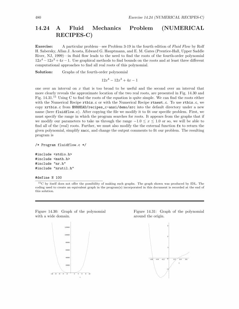
480 Exercise 14.24 (NUMERICAL RECIPES-C)
14.24 A Fluid Mechanics Problem (NUMERICALRECIPES-C)
Exercise: A particular problem—see Problem 3-19 in the fourth edition of Fluid Flow by RolfH. Sabersky, Allan J. Acosta, Edward G. Hauptmann, and E. M. Gates (Prentice-Hall, Upper SaddleRiver, NJ, 1999)—in fluid flow leads to the need to find the roots of the fourth-order polynomial12x4−12x3 + 4x−1. Use graphical methods to find bounds on the roots and at least three differentcomputational approaches to find all real roots of this polynomial.
Solution: Graphs of the fourth-order polynomial
12x4 − 12x3 + 4x− 1
one over an interval on x that is too broad to be useful and the second over an interval thatmore clearly reveals the approximate location of the two real roots, are presented in Fig. 14.30 andFig. 14.31.15 Using C to find the roots of the equation is quite simple. We can find the roots eitherwith the Numerical Recipe rtbis.c or with the Numerical Recipe rtnewt.c. To use rtbis.c, wecopy xrtbis.c from $NRHEAD/recipes_c-ansi/demo/src into the default directory under a newname (here fluidflow.c). After copying the file we modify it to fit our specific problem. First, wemust specify the range in which the program searches for roots. It appears from the graphs that ifwe modify our parameters to take us through the range −1.0 ≤ x ≤ 1.0 or so, we will be able tofind all of the (real) roots. Further, we must also modify the the external function fx to return thegiven polynomial, simplify xacc, and change the output comments to fit our problem. The resultingprogram is
/* Program fluidflow.c */
#include <stdio.h>
#include <math.h>
#include "nr.h"
#include "nrutil.h"
#define N 100
15C by itself does not offer the possibility of making such graphs. The graph shown was produced by IDL. Thecoding used to create an equivalent graph in the program(s) incorporated in this document is recorded at the end ofthis solution.
Figure 14.30: Graph of the polynomialwith a wide domain.
20000
40000
60000
80000
100000
120000
–10 –8 –6 –4 –2 2 4 6 8 10
x
Figure 14.31: Graph of the polynomialaround the origin.
–1
0
1
2
3
–0.6 –0.4 –0.2 0.2 0.4 0.6
x
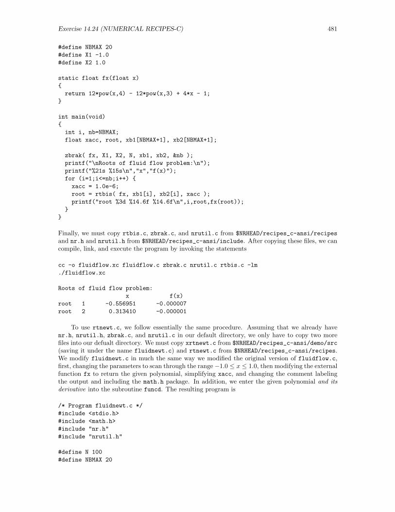
Exercise 14.24 (NUMERICAL RECIPES-C) 481
#define NBMAX 20
#define X1 -1.0
#define X2 1.0
static float fx(float x)
return 12*pow(x,4) - 12*pow(x,3) + 4*x - 1;
int main(void)
int i, nb=NBMAX;
float xacc, root, xb1[NBMAX+1], xb2[NBMAX+1];
zbrak( fx, X1, X2, N, xb1, xb2, &nb );
printf("\nRoots of fluid flow problem:\n");
printf("%21s %15s\n","x","f(x)");
for (i=1;i<=nb;i++)
xacc = 1.0e-6;
root = rtbis( fx, xb1[i], xb2[i], xacc );
printf("root %3d %14.6f %14.6f\n",i,root,fx(root));
Finally, we must copy rtbis.c, zbrak.c, and nrutil.c from $NRHEAD/recipes_c-ansi/recipes
and nr.h and nrutil.h from $NRHEAD/recipes_c-ansi/include. After copying these files, we cancompile, link, and execute the program by invoking the statements
cc -o fluidflow.xc fluidflow.c zbrak.c nrutil.c rtbis.c -lm
./fluidflow.xc
Roots of fluid flow problem:
x f(x)
root 1 -0.556951 -0.000007
root 2 0.313410 -0.000001
To use rtnewt.c, we follow essentially the same procedure. Assuming that we already havenr.h, nrutil.h, zbrak.c, and nrutil.c in our default directory, we only have to copy two morefiles into our defualt directory. We must copy xrtnewt.c from $NRHEAD/recipes_c-ansi/demo/src
(saving it under the name fluidnewt.c) and rtnewt.c from $NRHEAD/recipes_c-ansi/recipes.We modify fluidnewt.c in much the same way we modified the original version of fluidflow.c,first, changing the parameters to scan through the range −1.0 ≤ x ≤ 1.0, then modifying the externalfunction fx to return the given polynomial, simplifying xacc, and changing the comment labelingthe output and including the math.h package. In addition, we enter the given polynomial and itsderivative into the subroutine funcd. The resulting program is
/* Program fluidnewt.c */
#include <stdio.h>
#include <math.h>
#include "nr.h"
#include "nrutil.h"
#define N 100
#define NBMAX 20
482 Exercise 14.24 (NUMERICAL RECIPES-C)
#define X1 -1.0
#define X2 1.0
static float fx(float x)
return 12*pow(x,4) - 12*pow(x,3) + 4*x - 1;
static void funcd(float x,float *fn, float *df)
*fn = 12*pow(x,4) - 12*pow(x,3) + 4*x - 1;
*df = 48*pow(x,3) - 36*pow(x,2) + 4;
int main(void)
int i, nb = NBMAX;
float xacc, root, xb1[NBMAX+1], xb2[NBMAX+1];
zbrak(fx,X1,X2,N,xb1,xb2,&nb);
printf("\nRoots of fluid flow problem:\n");
printf("%21s %15s\n","x","f(x)");
for (i=1;i<=nb;i++)
xacc=(1.0e-6);
root=rtnewt(funcd,xb1[i],xb2[i],xacc);
printf("root %3d %14.6f %14.6f\n",i,root,fx(root));
Having already copied the necessary files to our default directory, we compile, link and execute theprogram with the statements
cc -o fluidnewt.xc fluidnewt.c zbrak.c nrutil.c rtnewt.c -lm
./fluidnewt.xc
Roots of fluid flow problem:
x f(x)
root 1 -0.556951 0.000000
root 2 0.313410 0.000000
From both programs we see that the two roots of the given fourth-order polynomial are−0.556951 and 0.313410.
IDL Code
x= -10.0 + 20.0*findgen(201)/200.0
y = 12.0*x^4 - 12.0*x^3+ 4.0*x-1.0
plot, x, y, thick=4
oplot, [-10.0, 10.0], [0.0,0.0], linestyle=2
x= -1.0 + 2.0*findgen(101)/100.0
y = 12.0*x^4 - 12.0*x^3+ 4.0*x-1.0
plot, x, y, thick=4
oplot, [-1.0, 1.0], [0.0,0.0], linestyle=2
Exercise 14.30 (NUMERICAL RECIPES-C) 483
14.30 Finite Depth Square Well (NUMERICAL RECIPES-C)
Exercise: Study the demonstration programs xrtbis.c and xrtnewt.c, each of which iswritten so as to be able to find all roots of a given function in a specified range. Then recast eachof these programs to produce a program that will find all of the positive roots of the equation foreach sign in the equation
sin s = ±0.04 s or sin s∓ 0.04 s = 0
for a finite depth well. Write your program so that the value of c and the boundaries of the region inwhich roots are to be sought are entered from the terminal at the time the program is run. Finally,test your program with c = 25, comparing your results with those obtained in the text, and thenexamine other values of c, seeking ultimately to obtain a graph showing each root as a function of c.
Solution: We examine the way that the energy levels of a quantum well change as the depthand width of the well (specified by c) change. As described in CPSUP Section 12.1.5, the value ofs for an allowed energy level must satisfy the equation
s cot(s) = −√c2 − s2
We can simplify this equation, as is done in Section 12.1.5, by squaring it, finding that the values ofs for allowed energy levels are the roots of the expression
sin(s)∓ s
c= 0
Note however that, by simplifying the expression, we have possibly introduced spurious roots, so wemust ultimately check the roots in the original equation.
We can find the roots of our equation in FORTRAN using either the Numerical Recipe rtbis.cand a corresponding driving program or the Numerical Recipe rtnewt.c and a corresponding drivingprogram.
Solution using rtbis.c:
To use rtbis.c, we must copy several files into our default directory. First, we copy thedemonstration program xrtbis.c from $NRHEAD/recipes_c-ansi/demo/src and save it under anappropriate name (here qwell.c). Then, we modify this file to fit our specific problem by
• changing all variables whose names begin with x to variables with names beginning with s (soas to facilitate correlation of the program with the statement of the problem).
• defining the function whose roots are to be found with the statements
static float fs( float s)
return sin(s)+aj*s/c;
where we have introduced the variable aj, which will be given the value +1 or the value −1as a means to combine both signs in the above equation into a single program, and we definethe variables aj and c as global variables with the statement
float c, j;
placed outside the main program so values set in the main program can be communicated tothe function without placing them as explicit arguments to the function.Further, we add thestatements
484 Exercise 14.30 (NUMERICAL RECIPES-C)
printf("\n Enter a value for c: " );
scanf("%f", &c);
printf("\n Enter -1 for an upper solution and 1 for a lower solution: " );
scanf("%f", &aj);
to the main program so that values of c and aj can be entered at execution time.
• deleting the arguments s1 and s2 of the #define directives that specify the range of the searchand adding the statements
printf("\n Enter a value for the lower boundary: " );
scanf("%f", &s1);
printf("\n Enter a value for the upper boundary: " );
scanf("%f", &s2);
so that the range will be specified by the user at execution time. (Note that a search startedat the value s = 0 will generate an error message. We seek only positive roots, but we will,when the time comes, start each search at s = −0.5 to avoid the problem just mentioned.)
• arranging for writing the results into a file for transfer to a graphing program by defining thecharacter variable filename and reading its value at execution time with the statements
char filename[20];
printf("\n Enter an appropriate file name (must be less than 20
characters and end in .dat): " );
scanf( "%s", filename );
fptr = fopen( filename, "w" );
We must, of course, also modify the output statement to write to this file rather than to thescreen and then, after all output has been produced, we must close the file.
These provisions allow the user to run the program multiple times without having to recompile it.The resulting program is
/* Program qwell.c */
#include <stdio.h>
#include "nr.h"
#include "nrutil.h"
#include <math.h>
#include <string.h>
#define N 100
#define NBMAX 30
float c, aj;
static float fs( float s)
return sin(s)+aj*s/c;
int main(void)
Exercise 14.30 (NUMERICAL RECIPES-C) 485
float s1, s2;
char filename[20];
int i, nb=NBMAX;
float sacc, root, sb1[NBMAX+1], sb2[NBMAX+1];
FILE *fptr;
printf("\n Enter a value for the lower boundary: " );
scanf("%f", &s1);
printf(" Enter a value for the upper boundary: " );
scanf("%f", &s2);
printf(" Enter a value for c: " );
scanf("%f", &c);
printf(" Enter -1 for an upper solution and 1 for a lower solution: " );
scanf("%f", &aj);
printf(" Enter an appropriate file name (must be less than 20\n" );
printf(" characters and end in .dat): " );
scanf("%s", filename );
zbrak(fs,s1,s2,N,sb1,sb2,&nb);
fptr = fopen( filename, "w" );
for (i=1;i<=nb;i++)
sacc=(1.0e-6);
root=rtbis(fs,sb1[i],sb2[i],sacc);
fprintf(fptr, "%14.6f\n",root);
fclose(fptr);
return 0;
Next, we must copy the files nr.h and nrutil.h from $NRHEAD/recipes_c-ansi/include intoour default directory. Finally, we must copy the files rtbis.c, nrutil.c, and zbrak.c from$NRHEAD/recipes_c-ansi/recipes into our default directory and compile qwell.c (along withrtbis.c and zbrak.c) with the statement
cc -o qwell.xc qwell.c zbrak.c nrutil.c rtbis.c -lm
Once the executable file qwell.xc is available, we run the program many times with differentvalues of c and different filenames. For example, with c = 2.0, we would create files containing theroots for each sign with the input
./qwell.xc
Enter a value for the lower bound: -0.5
Enter a value for the upper bound: 60.0
Enter a value for c: 2.0
Enter -1 for an upper solution and 1 for a lower solution: -1
Enter an appropriate file name(ends in .dat
and is less than 20 characters): qwell02up_c.dat
./qwell.xc
Enter a value for the lower bound: -0.5
Enter a value for the upper bound: 60.0
Enter a value for c: 2.0
Enter -1 for an upper solution and 1 for a lower solution: 1
Enter an appropriate file name(ends in .dat
and is less than 20 characters): qwell02lo_c.dat
486 Exercise 14.30 (NUMERICAL RECIPES-C)
In similar fashion, We run the program many times to obtain the results for several values of c,including c = 5, 10, 25, and 50. Each time we run the program we enter a different filename as theoutput location for the data, changing in particular the sixth and seventh characters to reflect thevalue of c to which the file applies. In particular, by displaying these files, we find that the roots(some of which are spurious) for c = 2 are
upper: -0.000000 lower: -0.000000
1.895495
and those for c = 25 are
upper: -0.000000 lower: -0.000000
3.020478 3.272885
6.548204 6.039204
9.054186 9.828837
13.118793 12.062847
15.061390 16.424786
19.761087 18.043257
20.994287 23.177780
23.864494
Graphing Solution with IDL
To create the energy level diagram with IDL, we begin by opening our file and storing the datain an array with the statements
IDL> openr, 1, ’qwell02up_c.dat’
IDL> upper2 = fltarr(2,1)
IDL> readf, 1, upper2
IDL> close, 1
IDL> print, upper2
-1.00000e-06 1.89550
where qwell02up_c.dat is the name of the file where our data are stored. Note that we executethe statements for c = 2 to begin with. This is a special case and a more general routine appearsjust after this specific routine. We do not open the qwell02lo_c.dat file in IDL because we knowthat the only root in that file is zero and we know that it is a spurious root. However, for all othersubsequent routines (as shown later) we will also open the lower solution file. Furthermore, notethat the size of the array needed to store the data will vary for the upper and lower solutions as wellas for each value of c. To find the appropriate size for the array, the data file must be opened andlooked at. After creating the arrays in IDL we want to combine the upper and lower solutions as wellas weed out the spurious solutions. We begin by eliminating the spurious solutions. To accomplishthis task we plug the solutions back into the equation
s cot(s) = −√c2 − s2
with the statement
IDL> print, upper2*cos(upper2)/sin(upper2) + sqrt(2.0^2 -upper2^2)
3.00000 -4.29153e-06
Only those roots which produce a result of zero (within the precision of our determination of theroot) are acceptable solutions. We then combine the acceptable upper and lower solutions into asingle array and plug that array into the equation for E/V0
E/V0 = −(1− s2/c2)
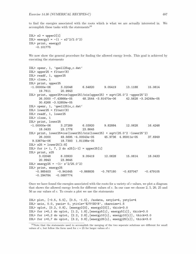
Exercise 14.30 (NUMERICAL RECIPES-C) 487
to find the energies associated with the roots which is what we are actually interested in. Weaccomplish these tasks with the statements16
IDL> s2 = upper2[1]
IDL> energy2 = -(1 - s2^2/2.0^2)
IDL> print, energy2
-0.101775
We now show the general procedure for finding the allowed energy levels. This goal is achieved byexecuting the statements
IDL> openr, 1, ’qwell25up_c.dat’
IDL> upper25 = fltarr(8)
IDL> readf, 1, upper25
IDL> close, 1
IDL> print, upper25
-1.00000e-06 3.02048 6.54820 9.05419 13.1188 15.0614
19.7611 20.9943
IDL> print, upper25*cos(upper25)/sin(upper25) + sqrt(25.0^2 -upper25^2)
26.0000 -7.43866e-05 48.2544 -3.81470e-06 42.5628 -3.24249e-05
30.6268 -3.52859e-05
IDL> openr, 1, ’qwell25lo_c.dat’
IDL> lower25 = fltarr(9)
IDL> readf, 1, lower25
IDL> close, 1
IDL> print, lower25
-1.00000e-06 3.27289 6.03920 9.82884 12.0628 16.4248
18.0433 23.1778 23.8645
IDL> print, lower25*cos(lower25)/sin(lower25) + sqrt(25.0^2 -lower25^2)
26.0000 49.5695 -4.00543e-05 45.9736 4.95911e-05 37.6949
9.53674e-06 18.7393 1.81198e-05
IDL> s25 = lower25[1:8]
IDL> for i= 1, 7, 2 do s25[i-1] = upper25[i]
IDL> print, s25
3.02048 6.03920 9.05419 12.0628 15.0614 18.0433
20.9943 23.8645
IDL> energy25 = -(1- s^2/25.0^2)
IDL> print, energy25
-0.985403 -0.941645 -0.868835 -0.767180 -0.637047 -0.479105
-0.294784 -0.0887774
Once we have found the energies associated with the roots for a variety of c values, we plot a diagramthat shows the allowed energy levels for different values of c. In our case we choose 2, 5, 20, 25 and50 as our values of c. To create a plot we use the statements
IDL> plot, [-0.5, 5.5], [0.5, -1.5], /nodata, xstyle=4, ystyle=4
IDL> axis, 0.0, yaxis= 0, ytitle=’E/V!DO!N’, charsize=1.5
IDL> oplot, [0.2, 0.8], [energy2[0], energy2[0]], thick=3.0
IDL> for i=0,1 do oplot, [1.2, 1.8],[energy5[i], energy5[i]], thick=3.0
IDL> for i=0,2 do oplot, [2.2, 2.8],[energy10[i], energy10[i]], thick=3.0
IDL> for i=0,7 do oplot, [3.2, 3.8],[energy25[i], energy25[i]], thick=3.0
16Note that the statements used to accomplish the merging of the two seperate solutions are different for smallvalues of c, but follow the form used for c = 25 for larger values of c
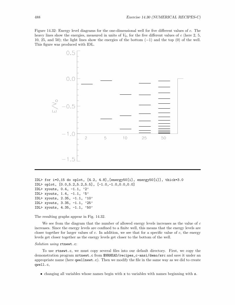
488 Exercise 14.30 (NUMERICAL RECIPES-C)
Figure 14.32: Energy level diagrams for the one-dimensional well for five different values of c. Theheavy lines show the energies, measured in units of V0, for the five different values of c (here 2, 5,10, 25, and 50); the light lines show the energies of the bottom (−1) and the top (0) of the well.This figure was produced with IDL.
IDL> for i=0,15 do oplot, [4.2, 4.8],[energy50[i], energy50[i]], thick=3.0
IDL> oplot, [0.0,5.2,5.2,5.5], [-1.0,-1.0,0.0,0.0]
IDL> xyouts, 0.4, -1.1, ’2’
IDL> xyouts, 1.4, -1.1, ’5’
IDL> xyouts, 2.35, -1.1, ’10’
IDL> xyouts, 3.35, -1.1, ’25’
IDL> xyouts, 4.35, -1.1, ’50’
The resulting graphs appear in Fig. 14.32.
We see from the diagram that the number of allowed energy levels increases as the value of cincreases. Since the energy levels are confined to a finite well, this means that the energy levels arecloser together for larger values of c. In addition, we see that for a specific value of c, the energylevels get closer together as the energy levels get closer to the bottom of the well.
Solution using rtnewt.c:
To use rtnewt.c, we must copy several files into our default directory. First, we copy thedemonstration program xrtnewt.c from $NRHEAD/recipes_c-ansi/demo/src and save it under anappropriate name (here qwellnewt.c). Then we modify the file in the same way as we did to createqwell.c,
• changing all variables whose names begin with x to variables with names beginning with s.
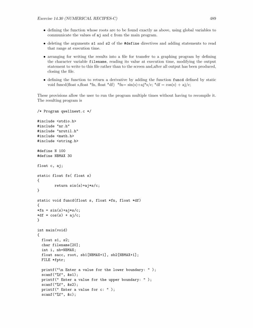
Exercise 14.30 (NUMERICAL RECIPES-C) 489
• defining the function whose roots are to be found exactly as above, using global variables tocommunicate the values of aj and c from the main program.
• deleting the arguments s1 and s2 of the #define directives and adding statements to readthat range at execution time.
• arranging for writing the results into a file for transfer to a graphing program by definingthe character variable filename, reading its value at execution time, modifying the outputstatement to write to this file rather than to the screen and,after all output has been produced,closing the file.
• defining the function to return a derivative by adding the function funcd defined by staticvoid funcd(float s,float *fn, float *df) *fn= sin(s)+aj*s/c; *df = cos(s) + aj/c;
These provisions allow the user to run the program multiple times without having to recompile it.The resulting program is
/* Program qwellnewt.c */
#include <stdio.h>
#include "nr.h"
#include "nrutil.h"
#include <math.h>
#include <string.h>
#define N 100
#define NBMAX 30
float c, aj;
static float fs( float s)
return sin(s)+aj*s/c;
static void funcd(float s, float *fn, float *df)
*fn = sin(s)+aj*s/c;
*df = cos(s) + aj/c;
int main(void)
float s1, s2;
char filename[20];
int i, nb=NBMAX;
float sacc, root, sb1[NBMAX+1], sb2[NBMAX+1];
FILE *fptr;
printf("\n Enter a value for the lower boundary: " );
scanf("%f", &s1);
printf(" Enter a value for the upper boundary: " );
scanf("%f", &s2);
printf(" Enter a value for c: " );
scanf("%f", &c);
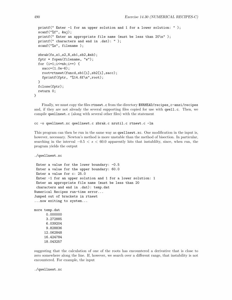
490 Exercise 14.30 (NUMERICAL RECIPES-C)
printf(" Enter -1 for an upper solution and 1 for a lower solution: " );
scanf("%f", &aj);
printf(" Enter an appropriate file name (must be less than 20\n" );
printf(" characters and end in .dat): " );
scanf("%s", filename );
zbrak(fs,s1,s2,N,sb1,sb2,&nb);
fptr = fopen(filename, "w");
for (i=1;i<=nb;i++)
sacc=(1.0e-6);
root=rtnewt(funcd,sb1[i],sb2[i],sacc);
fprintf(fptr, "%14.6f\n",root);
fclose(fptr);
return 0;
Finally, we must copy the files rtnewt.c from the directory $NRHEAD/recipes_c-ansi/recipes
and, if they are not already the several supporting files copied for use with qwell.c. Then, wecompile qwellnewt.c (along with several other files) with the statement
cc -o qwellnewt.xc qwellnewt.c zbrak.c nrutil.c rtnewt.c -lm
This program can then be run in the same way as qwellnewt.xc. One modification in the input is,however, necessary. Newton’s method is more unstable than the method of bisection. In particular,searching in the interval −0.5 < s < 60.0 apparently hits that instablilty, since, when run, theprogram yields the output
./qwellnewt.xc
Enter a value for the lower boundary: -0.5
Enter a value for the upper boundary: 60.0
Enter a value for c: 25.0
Enter -1 for an upper solution and 1 for a lower solution: 1
Enter an appropriate file name (must be less than 20
characters and end in .dat): temp.dat
Numerical Recipes run-time error...
Jumped out of brackets in rtnewt
...now exiting to system...
more temp.dat
0.000000
3.272885
6.039204
9.828836
12.062848
16.424784
18.043257
suggesting that the calculation of one of the roots has encountered a derivative that is close tozero somewhere along the line. If, however, we search over a different range, that instability is notencountered. For example, the input
./qwellnewt.xc

Exercise 14.30 (NUMERICAL RECIPES-C) 491
Enter a value for the lower boundary: -2.0
Enter a value for the upper boundary: 60.0
Enter a value for c: 25.0
Enter -1 for an upper solution and 1 for a lower solution: 1
Enter an appropriate file name (must be less than 20
characters and end in .dat): temp.dat
yields no error message and finds the roots
more temp.dat
0.000000
3.272885
6.039204
9.828836
12.062848
16.424784
18.043257
23.177778
23.864494
Once we find ways to avoid this instability, the output is the same in all cases as that obtained bythe method of bisection, and we suppress any further discussion or processing of that output.


Appendix A
Introduction to LATEX
A.2 A Letter to a Friend
Exercise: Use LATEX to write a letter to a friend. Format your letter so that it has
• a centered block at the top containing your name and address (center environment);
• a right-justified date (using \today and either \hfill or the flushright environment);
• a left-justified block containing an inside address (flushleft environment);
• a left-justified salutation;
• the body of the letter, containing more than one paragraph;
• a closing (e.g., Sincerely, With love, . . .) positioned 3.5” from the left margin; and
• your name, spaced far enough below the closing to allow for your signature and aligned withthe closing.
Suppress page numbers altogether on this letter. Include both your LATEX code and the processedoutput in what you submit as a solution to this exercise.
Solution: I begin by creating the preamble, including selection of 11 point type, with thecoding
\documentclass[11pt]article
% Set size of text area, size of page, position of printed
% area on page, extra space between paragraphs, paragraph
% indent.
\setlength\textheight9.0truein % Set 6"x9" print area
\setlength\textwidth6.0truein
\setlength\topmargin-0.5truein % Set 1" top margin
\setlength\parskip6pt plus 2pt minus 1pt % Specify extra 5-8pt space
% between paragraphs
\setlength\parindent20pt % Set 20-pt paragraph indent
\pagestyleempty % Suppress page numbers
\begindocument
493
494 Exercise A.2
Then, I create the letterhead and specify the inside address, the current date, and the salutationwith the coding
\begincenter
David M. Cook \\
Department of Physics \\
Lawrence University \\
711 E Boldt Way \\
Appleton, WI 54911
\endcenter
\beginflushright
\today
\endflushright
\beginflushleft
Professor Richard Feynman \\
Department of Physics \\
California Institute of Technology \\
1200 E California Blvd \\
Pasadena, CA 91125
\endflushleft
\noindent Dear Professor Feynman,
Next, I create the body of the letter. Appropriate in a letter to Richard Feynman, I choose toinclude some mathematical symbols and a couple of equations, partly to illustrate how to do that.The body of the letter is achieved with the coding
I seek your confirmation on the correctness of two equations. First, I understand
that the allowed energies $E$ of a quantum particle of mass $m$ moving in
one dimension under the influence of a spring of constant $k$ are the
eigenvalues of the time-independent Schr\"odinger equation
\beginequation
\labelschr
-\frac\hbar^22m\fracd^2\psi(x)dx^2 + \frac12kx^2\psi(x) = E\psi(x)
\endequation
Here, $\psi(x)$ is the wave function of the particle. This equation is to be
solved subject to the boundary conditions that $\psi(\pm\infty) = 0$.
Second, I understand that the product $\mathbfC$ of two matrices $\mathbfA$
and $\mathbfB$, the first of which has the same number of columns as the
second of which has rows has elements given by
\beginequation
\labelmatmul
\mathbfC = \mathbfA\mathbfB \qquad \Longrightarrow \qquad C_\mu\nu =
\sum_i=1^N A_\mu i\,B_i\nu
\endequation
Here, $N$ is the (common) number of columns in $\mathbfA$ and the number of
rows in $\mathbfB$.
I will postpone further studies based on Eqs.~(\refschr) and (\refmatmul)
until you confirm their correctness. Thank you very much.
Finally, I add the salutation and complete the file with the coding
Exercise A.2 495
\hspace3.5truein \parbox2.4trueinSincerely, \\[36pt]
David M. Cook
\enddocument
The specification [36pt] at the end of the closing assures sufficient space between the closing andthe typed name for a hand-written signature.
The completed file, stored with the name letter-ex02.tex is listed below:
The file letter-ex02.tex that solves Exercise A.2.
\documentclass[11pt]article
% Set size of text area, size of page, position of printed
% area on page, extra space between paragraphs, paragraph
% indent.
\setlength\textheight9.0truein % Set 6"x9" print area
\setlength\textwidth6.0truein
\setlength\topmargin-0.5truein % Set 1" top margin
\setlength\parskip6pt plus 2pt minus 1pt % Specify extra 5-8pt space
% between paragraphs
\setlength\parindent20pt % Set 20-pt paragraph indent
\pagestyleempty % Suppress page numbers
\begindocument
\begincenter
David M. Cook \\
Department of Physics \\
Lawrence University \\
711 E Boldt Way \\
Appleton, WI 54911
\endcenter
\beginflushright
\today
\endflushright
\beginflushleft
Professor Richard Feynman \\
Department of Physics \\
California Institute of Technology \\
1200 E California Blvd \\
Pasadena, CA 91125
\endflushleft
\noindent Dear Professor Feynman,
I seek your confirmation on the correctness of two equations. First, I understand
that the allowed energies $E$ of a quantum particle of mass $m$ moving in
one dimension under the influence of a spring of constant $k$ are the
eigenvalues of the time-independent Schr\"odinger equation
\beginequation
496 Exercise A.2
\labelschr
-\frac\hbar^22m\fracd^2\psi(x)dx^2 + \frac12kx^2\psi(x) = E\psi(x)
\endequation
Here, $\psi(x)$ is the wave function of the particle. This equation is to be
solved subject to the boundary conditions that $\psi(\pm\infty) = 0$.
Second, I understand that the product $\mathbfC$ of two matrices $\mathbfA$
and $\mathbfB$, the first of which has the same number of columns as the
second of which has rows has elements given by
\beginequation
\labelmatmul
\mathbfC = \mathbfA\mathbfB \qquad \Longrightarrow \qquad C_\mu\nu =
\sum_i=1^N A_\mu i\,B_i\nu
\endequation
Here, $N$ is the number of columns in $\mathbfA$ and the number of
rows in $\mathbfB$.
I will postpone further studies based on Eqs.~(\refschr) and (\refmatmul)
until you confirm their correctness. Thank you very much.
\noindent \hspace3.5truein \parbox2.4trueinSincerely, \\[36pt]
David M. Cook
\enddocument
With this file stored in the default directory, the pdf file containing the formatted text can thenbe created with the two simple statements1
pdflatex letter-ex02
pdflatex letter-ex02
which also creates the additional files letter-ex02.aux and letter-ex02.log and the desired fileletter-ex02.pdf. Unfortunately, in the first pass, the internal references to the two equationswill not be identified. That information is written into the file letter-ex02.aux in that pass.In the second pass, that file is read and provides the information to resolve those two internalreferences. Anytime a file contains internal references, at least two (and sometimes three) passesthrough pdflatex will be necessary. Printing of the file letter-ex02.pdf creates the letter shownon the next page.
1At Lawrence, the system is set so that, no matter the default directory, the system will find pdflatex without apath specification. At other sites, a different statement may be necessary.
Exercise A.2 497
David M. CookDepartment of PhysicsLawrence University
711 E Boldt WayAppleton, WI 54911
November 28, 2020
Professor Richard FeynmanDepartment of PhysicsCalifornia Institute of Technology1200 E California BlvdPasadena, CA 91125
Dear Professor Feynman,
I seek your confirmation on the correctness of two equations. First, I understand thatthe the allowed energies E of a quantum particle of mass m moving in one dimensionunder the influence of a spring of constant k are the eigenvalues of the time-independentSchrodinger equation
− h2
2m
d2ψ(x)
dx2+
1
2kx2ψ(x) = Eψ(x) (1)
Here, ψ(x) is the wave function of the particle. This equation is to be solved subject to theboundary conditions that ψ(±∞) = 0.
Second, I understand that the product C of two matrices A and B, the first of whichhas the same number of columns as the second of which has rows has elements given by
C = AB =⇒ Cµν =N∑i=1
AµiBiν (2)
Here, N is the number of columns in A and the number of rows in B.
I will postpone further studies based on Eqs. (1) and (2) until you confirm their cor-rectness. Thank you very much.
Sincerely,
David M. Cook
498 Exercise A.4
A.4 Chain Radioactive Decay
Exercise: The folder $HEAD/tex contains the three files radio.ps, radio.eps, and radio.pdf,each of which contains a description of a graph showing the number of nuclei of each of three speciesA, B, and C as a function of time as the 1000 nuclei of A initially present decay radioactively firstto B and then to C. The equations describing the system are
dA
dt= −kAA ;
dB
dt= kAA− kBB ;
dC
dt= kBB
and the graph shows the solution of these equations when the initial conditions are A(0) = 1000,B(0) = C(0) = 0 for the case kA = kB = 0.1. Prepare a document containing this figure, thedifferential equations, the initial conditions, and a brief description of the graph in English. Be surethat your text includes explicit references to the figure and the equations. You might also contriveto include a footnote somewhere. Include both your LATEX code and the processed output in whatyou submit as a solution to this exercise. A Crutch: The file $HEAD/tex/sampledoc.tex providesa start on the creation of a suitable source file for this exercise.
Solution: I begin by copying the file radio.pdf to the default directory. Then I create thepreamble, including selection of 11 point type and incorporation of the graphicx package, with thecoding
\documentclass[11pt]article
% Set size of text area, size of page, position of printed
% area on page, extra space between paragraphs, paragraph
% indent.
\setlength\textheight9.0truein % Set 6"x9" print area
\setlength\textwidth6.0truein
\setlength\topmargin-0.5truein % Set 1" top margin
\setlength\parskip6pt plus 2pt minus 1pt % Specify extra 5-8pt space
% between paragraphs
\setlength\parindent20pt % Set 20-pt paragraph indent
\pagestyleempty % Suppress page numbers
\usepackagegraphicx
\begindocument
Next, I add a title and a descriptive text with the coding
\begincenter
\large\bf Solution to Exercise A.4 in CPSUP
\endcenter
Let $A(t)$, $B(t)$, and $C(t)$ represent in some units the the quantity of
three chemical species present in a reaction vessel. Suppose that $C$ is
stable but that $A$ decays to $B$ and $B$ to $C$ according to the equations
\beginequation
\labeldecay
\fracdAdt = -k_AA \quad ; \quad \fracdBdt = k_AA - k_BB \quad ; \quad
\fracdCdt
\endequation
where the constants $k_A$ and $k_B$ Suppose further that, initially 1000
Exercise A.4 499
units of $A$ are present but $B$ and $C$ are absent to that the initial
conditions for the behavior of this system are
\beginequation
\labelics
A(0) = 1000 \quad ; \quad B(0) = 0 \quad ; \quad C(0) = 0
\endequartion
The result of a numerical solution of the three ordinary differential
equations Eqs.~\refdecay subject to the initial conditions in
Eq.~\refics when $k_A = k_B = 0.1$ is shown in Fig.~\refdecaygr.
Finally, we incorporate the graph and end the file with the coding2
\beginfigure[h]
\captionBehavior of a three-atom chain radioactive decay.
\labeldecaygr
\includegraphics[height=3.5truein]radio
\endfigure
\enddocument
Note that the quantity of A steadily goes down; that the quantity of B rises initially when it isproduced by decay of A faster than it decays to C; but finally as B’s rate of production diminishes(because the quantity of A is reduced), it decays to C faster than it is produced; and the quantityof C rises steadily until, after a long time, all of A has been converted to C and there is no B lefteither.
The completed file, stored with the name letter-ex02.tex is listed below:
The file decay-ex04.tex that solves Exercise A.4.
\documentclass[11pt]article
% Set size of text area, size of page, position of printed
% area on page, extra space between paragraphs, paragraph
% indent.
\setlength\textheight9.0truein % Set 6"x9" print area
\setlength\textwidth6.0truein
\setlength\topmargin-0.5truein % Set 1" top margin
\setlength\parskip6pt plus 2pt minus 1pt % Specify extra 5-8pt space
% between paragraphs
\setlength\parindent20pt % Set 20-pt paragraph indent
\pagestyleempty % Suppress page numbers
\usepackagegraphicx
\begindocument
\begincenter
\large\bf Solution to Exercise A.4 in CPSUP
\endcenter
2Here, the designation [h] at the end of the first line overrides the default positioning of the figure at the top ofthe page to place it “here”, i.e., right after the last line of text.
500 Exercise A.4
Let $A(t)$, $B(t)$, and $C(t)$ represent in some units the the quantity of
three chemical species present in a reaction vessel. Suppose that $C$ is
stable but that $A$ decays to $B$ and $B$ to $C$ according to the equations
\beginequation
\labeldecay
\fracdAdt = -k_AA \quad ; \quad \fracdBdt = k_AA - k_BB \quad ; \quad
\fracdCdt
\endequation
where the constants $k_A$ and $k_B$ Suppose further that, initially 1000
units of $A$ are present but $B$ and $C$ are absent to that the initial
conditions for the behavior of this system are
\beginequation
\labelics
A(0) = 1000 \quad ; \quad B(0) = 0 \quad ; \quad C(0) = 0
\endequation
The result of a numerical solution of the three ordinary differential
equations in Eq.~(\refdecay) subject to the initial conditions in
Eq.~(\refics) when $k_A = k_B = 0.1$ is shown in Fig.~\refdecaygr.
\beginfigure[h]
\captionBehavior of a three-atom chain radioactive decay. $A$ is the
solid line, $B$ is the dotted line, and $C$ is the dashed line.
\labeldecaygr
\begincenter
\includegraphics[height=3.5truein]radio
\endcenter
\endfigure
\enddocument
With this file stored in the default directory, the pdf file containing the formatted text can thenbe created with the two simple statements3
pdflatex decay-ex04
pdflatex decay-ex04
which also creates the additional files decay-ex04.aux and decay-ex04.log and the desired filedecay-ex04.pdf. Unfortunately, in the first pass, the internal references to the two equationsand the figure will not be identified. That information is written into the file decay-ex04.aux inthat pass. In the second pass, that file is read and provides the information to resolve those threeinternal references. Anytime a file contains internal references, at least two (and sometimes three)passes through pdflatex will be necessary. Printing of the file decay-ex04.pdf creates the outputshown on the next page.
3At Lawrence, the system is set so that, no matter the default directory, the system will find pdflatex without apath specification. At other sites, a different statement may be necessary.
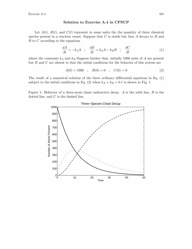
Exercise A.4 501
Solution to Exercise A.4 in CPSUP
Let A(t), B(t), and C(t) represent in some units the the quantity of three chemicalspecies present in a reaction vessel. Suppose that C is stable but that A decays to B andB to C according to the equations
dA
dt= −kAA ;
dB
dt= kAA− kBB ;
dC
dt(1)
where the constants kA and kB Suppose further that, initially 1000 units of A are presentbut B and C are absent to that the initial conditions for the behavior of this system are
A(0) = 1000 ; B(0) = 0 ; C(0) = 0 (2)
The result of a numerical solution of the three ordinary differential equations in Eq. (1)subject to the initial conditions in Eq. (2) when kA = kB = 0.1 is shown in Fig. 1.
Figure 1: Behavior of a three-atom chain radioactive decay. A is the solid line, B is thedotted line, and C is the dashed line.
0 10 20 30 40 500
100
200
300
400
500
600
700
800
900
1000Three−Species Chain Decay
Time
Num
ber
of A
tom
s P
rese
nt
Related Documents