This PDF is a selection from an out-of-print volume from the National Bureau of Economic Research Volume Title: The Microstructure of Foreign Exchange Markets Volume Author/Editor: Jeffrey A. Frankel, Giampaolo Galli, Alberto Giovannini, editors Volume Publisher: University of Chicago Press Volume ISBN: 0-226-26000-3 Volume URL: http://www.nber.org/books/fran96-1 Conference Date: July 1-2, 1994 Publication Date: January 1996 Chapter Title: Exchange Rate Economics: What's Wrong with the Conventional Macro Approach? Chapter Author: Robert P. Flood, Mark P. Taylor Chapter URL: http://www.nber.org/chapters/c11368 Chapter pages in book: (p. 261 - 302)

Welcome message from author
This document is posted to help you gain knowledge. Please leave a comment to let me know what you think about it! Share it to your friends and learn new things together.
Transcript

This PDF is a selection from an out-of-print volume from the NationalBureau of Economic Research
Volume Title: The Microstructure of Foreign Exchange Markets
Volume Author/Editor: Jeffrey A. Frankel, Giampaolo Galli, AlbertoGiovannini, editors
Volume Publisher: University of Chicago Press
Volume ISBN: 0-226-26000-3
Volume URL: http://www.nber.org/books/fran96-1
Conference Date: July 1-2, 1994
Publication Date: January 1996
Chapter Title: Exchange Rate Economics: What's Wrong with theConventional Macro Approach?
Chapter Author: Robert P. Flood, Mark P. Taylor
Chapter URL: http://www.nber.org/chapters/c11368
Chapter pages in book: (p. 261 - 302)
8 Exchange Rate Economics:What's Wrong with theConventional Macro Approach?Robert P. Flood and Mark P. Taylor
To include a paper entitled as this one is in a volume devoted to an examinationof the importance of market microstructure in foreign exchange markets is,to utilize a well-used phrase, to preach to the converted. The poor empiricalperformance of the major exchange rate models over the recent float is, more-over, extremely well documented (Frankel and Rose 1994; MacDonald andTaylor 1992; Taylor 1994). Nevertheless, it is important to have a formal state-ment of the theory and evidence relating to exchange rate models based onmacroeconomic fundamentals as a ground-clearing exercise since only by stat-ing what is wrong with the conventional macro approach can we hope to designmodels that fill the gaps left by the macro-based models. Thus, section 8.1 ofthis paper is devoted to a discussion of the theory and empirical evidence relat-ing to the major macroeconomic exchange rate models developed during thelast twenty years or so, including the flexible-price monetary model, the sticky-price, overshooting monetary model, the portfolio balance model, and the equi-librium model. In section 8.2, we provide a brief discussion of the theory andevidence relating to the speculative efficiency of foreign exchange markets.
Beyond this, however, we want to demonstrate that, while the macro funda-mentals are clearly not capable of explaining all—or even most—of the varia-tion in short-term nominal exchange rate movements, the research program ofthe last twenty years has nevertheless not been entirely fruitless. Our aim isthus to examine the macro fundamentals as a means of "setting the parameters"within which microstructural models might be constructed. Thus, in section
Robert P. Flood is a senior economist in the Research Department of the International MonetaryFund. Mark P. Taylor is professor of economics at the University of Liverpool.
The authors are grateful for comments on earlier versions of the paper from Jeffrey Frankel,Andrew Rose, Lars Svensson, and other conference participants. The views represented in thepaper are those of the authors and are not necessarily those of the International Monetary Fund orof its member authorities.
261
262 Robert P. Flood and Mark P. Taylor
8.3, we invert the question posed in the title of this paper and ask, What's rightwith the conventional macro approach? Using data on twenty-one industrial-ized countries for the floating-rate period, we show that, while the macro fun-damentals may be a poor guide to variations in short-run exchange rate move-ments (where the short run is defined as one year or less), they maynevertheless have considerable explanatory power over longer horizons.
A final section concludes the discussion and tries to give an answer to thequestion that the title of this paper poses.
8.1 Theory and Evidence on Exchange Rate Models Based onMacro Fundamentals
In this section, we review briefly the theory and evidence pertaining to thefour major exchange rate models based on conventional macro fundamentals:the monetary model, the sticky-price monetary model, the equilibrium model,and the portfolio balance model.' The monetary model is the simplest of thefour and assumes that all goods are perfect substitutes, as are all interest-bearing assets, and that all markets clear continuously. The other three modelsrelax, in various ways, some of the strong assumptions made in the monetarymodel and in some cases make explicit previously unarticulated assumptions.The sticky-price model makes two big changes from the monetary model: itadds multiple goods and allows slow adjustment of nominal goods prices. Theequilibrium model also allows multiple goods, but it models asset preferencesas depending on the covariation of real asset returns with the marginal utilityof consumption for some assets and as determined by unmodeled constraintsfor other assets. Also, by paying explicit attention to individual and economy-wide constraints, the equilibrium model is intended to clarify the full effectsof various policy options. Typically, equilibrium models require continuousgoods market and asset market clearing. Portfolio balance models are distin-guished by their preferred specification of asset demands and are eclectic withrespect to goods market specifications. In portfolio balance models, differentinterest-bearing assets are not perfect substitutes so that uncovered interest rateparity does not hold and asset demands may be modeled along the lines sug-gested by Tobin (1969).
Evidently, these four classes of model are not mutually exclusive. They sharemany common structural elements, including the property that expectations ofthe future are potentially crucial for current decisions, and, more important,they all share the property that current and expected future macro fundamen-tals are always at the heart of exchange rate determination.
Prior to setting out the theory and evidence relating to these four models indetail, however, we consider what is probably the simplest and in many ways
1. Sections 8.1 and 8.2 draw on MacDonald and Taylor (1992) and Taylor (1994).
263 Exchange Rate Economics: What's Wrong with the Macro Approach?
the most fundamental link between the exchange rate and macroeconomic fun-damentals: purchasing power parity.
8.1.1 Purchasing Power Parity
Purchasing power parity (PPP) is one of the simplest macro fundamentalexchange rate models that one can imagine. Absolute purchasing power parityimplies that the exchange rate is equal to the ratio of the two relevant nationalprice levels; relative purchasing power parity posits that changes in the ex-change rate are equal to changes in relative national prices:
(1) s, = (p, - pt) + i.
and
(2) As, =
where sr denotes the logarithm of the spot exchange rate (domestic price offoreign currency), and pt and p* denote the logarithms of suitably normalizednational price levels for the domestic and foreign economies, respectively. Thedeviation from purchasing power parity is commonly referred to as the realexchange rate, defined here in logarithmic form:
(3) ^, = st- (p, - p*) = (=,.
The professional consensus on the validity of purchasing power parity hasshifted radically over the past two decades or so. Prior to the recent float, theconsensus appeared to support the existence of a fairly stable real exchangerate—that is to say, the variance of £, or ^ was thought of as small relative tothe variance in relative prices or relative inflation rates. The prevailing ortho-doxy of the early 1970s, largely associated with the monetary approach to theexchange rate, assumed the much stronger proposition of continuous purchas-ing power parity—that is, that the variance of £r or %t was identically equal tozero (see, e.g., Frenkel 1976; and Frenkel and Johnson 1978). Proponents ofearly monetary exchange rate models, moreover, argued that, while the ex-change rate may apparently diverge from PPP when conventional price indicesare used, the condition would be seen to hold if one could observe the "true"price indices that are relevant for deflating national monies, so that observedvariation in £f or ^ was really due to variation in measurement errors.
In the mid- to late 1970s, in the light of the very high variability of realexchange rates, this extreme position was largely abandoned as the variabilityin observed deviations from PPP became so large that it became clear that theycould not be due to measurement errors alone. Subsequently, studies publishedmostly in the 1980s, which could not reject the hypothesis of random-walkbehavior in real exchange rates—that £f or ir, followed a random walk (e.g.,Adler and Lehmann 1983)—reduced further the confidence in purchasing
264 Robert P. Flood and Mark P. Taylor
power parity and led to the rather widespread belief that PPP was of little useempirically and that real exchange rate movements were highly persistent.
More recently, in an extension of this literature, researchers have tested formore general mean reversion or stationarity of the real exchange (where thealternative hypothesis is a more general unit root process rather than specifi-cally a random walk) have interpreted the null hypothesis of stationarity asequivalent to the existence of long-run purchasing power parity. Relatedly, re-searchers have also allowed the slope coefficients on domestic and foreignprices to differ from unity by testing for cointegration between the nominalexchange rate and domestic and foreign prices. Early cointegration studiesgenerally reported a failure of significant mean reversion of the exchange ratetoward purchasing power parity for the recent floating experience (Taylor1988; Mark 1990) but were supportive of reversion toward purchasing powerparity notably for the interwar float (Taylor and McMahon 1988) and for theexchange rates of high-inflation countries (McNown and Wallace 1989). Veryrecent applied work on long-run purchasing power parity among the majorindustrialized economies has, however, been more favorable toward the long-run purchasing power parity hypothesis for the recent float (e.g., Cheung andLai 1993; Lothian and Taylor 1994). A number of authors have argued that thedata period for the recent float alone may simply be too short to provide anyreasonable degree of test power in the normal statistical tests for stationarityof the real exchange rate (e.g., Frankel 1990).
8.1.2 The Flexible-Price Monetary Model
The monetary approach to the exchange rate, which emerged as the domi-nant exchange rate model at the start of the recent float in the early 1970s (e.g.,Frenkel 1976), starts from the definition of the exchange rate as the relativeprice of two monies and attempts to model that relative price in terms of therelative supply of and demand for those monies. Assuming stable, log-linearmoney demand functions at home and abroad (all variables except interest ratesexpressed in logarithms), the demand for money, m, is assumed to depend lin-early on real income, y, the price level, p, and the level of the nominal interestrate, / (foreign variables are denoted by an asterisk). Assuming continuous pur-chasing power parity (£, = 0 in [1]), and substituting out for relative prices,it is straightforward to derive the fundamental equation of the flexible-pricemonetary model:
(4) st = mt- m* - K(yt - y) + 6(i, - i,'),
where K and 0 are the income elasticity and interest rate semielasticity of thedemand for money (here assumed equal at home and abroad for expositorypurposes). By invoking the uncovered interest parity condition, we can substi-tute Ase
t+l for (it — i*) in order to emphasize the forward-looking nature ofthe model:
265 Exchange Rate Economics: What's Wrong with the Macro Approach?
(5) *, = <!>, ^ + 1
where cj>; is the monetary fundamental given by
(6) cj>, = m, - m* - K(V, - y*).
The rational expectations solution to (5) is
where E[- \ Clt] denotes the mathematical expectation conditioned on the infor-mation set available at time t, (I,.2 It is well known from the rational expecta-tions literature, however, that equation (7) is only one solution to (5) from apotentially infinite set involving rational bubbles.
Note that the flexible-price monetary model is really just a purchasing powerparity model of the exchange rate, where the proximate force driving relativeprices is assumed to be relative excess demand for money.
The very high volatility of real exchange rates during the 1970s float, con-spicuously refuting the assumption of continuous purchasing power parity, ledto the development of two further models, the sticky-price monetary modeland the so-called equilibrium model. Both of these can be viewed as extensionsor modifications in some way of the flexible-price monetary model. Beforeexamining the empirical evidence on the flexible-price monetary model, wegive a brief exposition of the sticky-price monetary model.
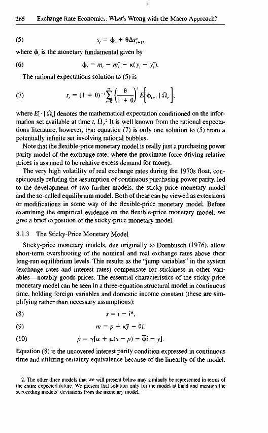
8.1.3 The Sticky-Price Monetary Model
Sticky-price monetary models, due originally to Dornbusch (1976), allowshort-term overshooting of the nominal and real exchange rates above theirlong-run equilibrium levels. This results as the "jump variables" in the system(exchange rates and interest rates) compensate for stickiness in other vari-ables—notably goods prices. The essential characteristics of the sticky-pricemonetary model can be seen in a three-equation structural model in continuoustime, holding foreign variables and domestic income constant (these are sim-plifying rather than necessary assumptions):
(8) s = i - i*,
(9) m = p + Ky - Qi,
(10) p = y[a + \x(s - p) - ijii - y].
Equation (8) is the uncovered interest parity condition expressed in continuoustime and utilizing certainty equivalence because of the linearity of the model.
2. The other three models that we will present below may similarly be represented in terms ofthe entire expected future. We present that solution only for the model at hand and mention thesucceeding models' deviations from the monetary model.
266 Robert P. Flood and Mark P. Taylor
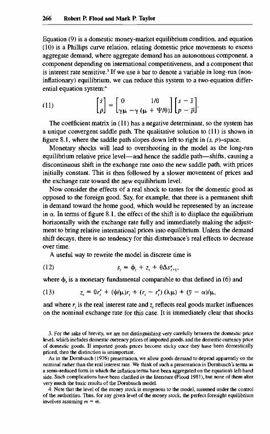
Equation (9) is a domestic money-market equilibrium condition, and equation(10) is a Phillips curve relation, relating domestic price movements to excessaggregate demand, where aggregate demand has an autonomous component, acomponent depending on international competitiveness, and a component thatis interest rate sensitive.3 If we use a bar to denote a variable in long-run (non-inflationary) equilibrium, we can reduce this system to a two-equation differ-ential equation system:4
f° 1/9 ]\s-'s
The coefficient matrix in (11) has a negative determinant, so the system hasa unique convergent saddle path. The qualitative solution to (11) is shown infigure 8.1, where the saddle path slopes down left to right in (s, /?)-space.
Monetary shocks will lead to overshooting in the model as the long-runequilibrium relative price level—and hence the saddle path—shifts, causing adiscontinuous shift in the exchange rate onto the new saddle path, with pricesinitially constant. This is then followed by a slower movement of prices andthe exchange rate toward the new equilibrium level.
Now consider the effects of a real shock to tastes for the domestic good asopposed to the foreign good. Say, for example, that there is a permanent shiftin demand toward the home good, which would be represented by an increasein a. In terms of figure 8.1, the effect of the shift is to displace the equilibriumhorizontally with the exchange rate fully and immediately making the adjust-ment to bring relative international prices into equilibrium. Unless the demandshift decays, there is no tendency for this disturbance's real effects to decreaseover time.
A useful way to rewrite the model in discrete time is
(12) sr = cj>, + z,
where cf>, is a monetary fundamental comparable to that defined in (6) and
(13) z, = 6r; + (i|i/n)r, + (r, - rj) (Xji) + (y -
and where rt is the real interest rate and z, reflects real goods market influenceson the nominal exchange rate for this case. It is immediately clear that shocks
3. For the sake of brevity, we are not distinguishing very carefully between the domestic pricelevel, which includes domestic currency prices of imported goods, and the domestic currency priceof domestic goods. If imported goods prices become sticky once they have been domesticallypriced, then the distinction is unimportant.
As in the Dornbusch (1976) presentation, we allow goods demand to depend apparently on thenominal rather than the real interest rate. We think of such a presentation in Dornbusch's terms asa semi-reduced form in which the inflation terms have been aggregated on the equation's left-handside. Such complications have been clarified in the literature (Flood 1981), but none of them altervery much the basic results of the Dornbusch model.
4. Note that the level of the money stock is exogenous to the model, assumed under the controlof the authorities. Thus, for any given level of the money stock, the perfect foresight equilibriuminvolves assuming m = m.

267 Exchange Rate Economics: What's Wrong with the Macro Approach?
p = 0
s = 0
Fig. 8.1 The saddle path for the sticky-price monetary model
and influence z, make the sticky-price monetary model's predictions divergefrom those of the flexible-price monetary model, at least in the short run. Tothe extent that shocks to zt are transitory, however, the differences between themonetary and the sticky-price models are transitory also.
8.1.4 Empirical Evidence on the Flexible-Price and Sticky-PriceMonetary Models
Initial support for the flexible-price monetary model was provided by Fren-kel (1976), who utilized data for the German mark/U.S. dollar exchange rateduring the German hyperinflation of the 1920s. The subsequent accumulationof data for the 1970s float allowed estimation of the model for the major ex-change rates during the recent float, and initial studies were also broadly sup-portive of the flexible-price monetary model (e.g., Bilson 1978; and Dornbusch1976). Beyond the late 1970s, however, the flexible-price monetary model (orits real interest differential variant) ceases to provide a good explanation ofvariations in exchange rate data: the estimated equations break down, provid-ing poor fits, exhibiting incorrectly signed coefficients, and failing generalequation diagnostics (e.g., Frankel 1993).
The evidence for the sticky-price monetary model is also weak when thedata period is extended beyond the late 1970s (Backus 1984). Another implica-tion of the sticky-price monetary model is proportional variation between thereal exchange rate and the real interest rate differential. This follows from thebasic assumptions of the overshooting model: slowly adjusting prices and un-covered interest rate parity. A number of studies have failed to find strong evi-dence of this relation, notably Meese and Rogoff (1988), who could not findcointegration between real exchange rates and real interest rate differentials.
268 Robert P. Flood and Mark P. Taylor
More recently, MacDonald and Taylor (1993, 1994) apply multivariate coin-tegration analysis and dynamic modeling techniques to a number of exchangerates and find some evidence to support the monetary model as a long-runequilibrium toward which the exchange rate converges, while allowing forcomplicated short-run dynamics. Since all the monetary models collapse to anequilibrium condition of the form (6) in the long run, these tests have no powerto discriminate between the alternative varieties. The usefulness of the cointe-gration approach suggested by these studies should, moreover, be taken as atmost tentative: their robustness across different data periods and exchangerates has yet to be demonstrated.
8.1.5 The Portfolio Balance Model
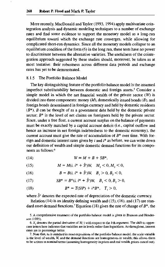
The key distinguishing feature of the portfolio balance model is the assumedimperfect substitutability between domestic and foreign assets.5 Consider asimple model in which the net financial wealth of the private sector (W) isdivided into three components: money (M), domestically issued bonds (B), andforeign bonds denominated in foreign currency and held by domestic residents(B*). B can be thought of as a government debt held by the domestic privatesector; B* is the level of net claims on foreigners held by the private sector.Since, under a free float, a current account surplus on the balance of paymentsmust be exactly matched by a capital account deficit (i.e., capital outflow andhence an increase in net foreign indebtedness to the domestic economy), thecurrent account must give the rate of accumulation of B* over time. With for-eign and domestic interest rates given by i and i* as before, we can write downour definition of wealth and simple domestic demand functions for its compo-nents as follows:6
(14) W = M + B + SB*,
(15) M = Mii, i* + Se)W, Ml <0,M2< 0,
(16) B = B(i, i* + Se)W, #, > 0, B2 < 0,
(17) SB* = B*(i, i* + Se)W, Bl <0,B2> 0,
(18) B* = T(S/P) + i*B*, r, > 0,
where Se denotes the expected rate of depreciation of the domestic currency.Relation (14) is an identity defining wealth and (15), (16), and (17) are stan-
dard asset demand functions.7 Equation (18) gives the rate of change of B*, the
5. A comprehensive treatment of the portfolio balance model is given in Branson and Hender-son (1985).
6. Xk denotes the partial derivative of X(-) with respect to the kth argument. The shift to upper-case letters here indicates that variables are in levels rather than logarithms. As throughout, interestrates are in percentage terms.
7. Note that, as is standard in most expositions of the portfolio balance model, the scale variableis the level of wealth, W, and the demand functions are homogeneous in wealth; this allows themto be written in nominal terms (assuming homogeneity in prices and real wealth, prices cancel out).

269 Exchange Rate Economics: What's Wrong with the Macro Approach?
capital account, as equal to the current account, which is in turn equal to thesum of the trade balance, T(-), and net debt service receipts, i*B*. The tradebalance depends positively on the level of the real exchange rate (a devaluationimproves the trade balance). The exchange rate is then determined by solvingequations (14)—(18) for given levels of M, B, and B*, normally assuming ratio-nal expectations. Disturbances to these stocks will result in movements in S inboth the short run (solve [14]—[18] allowing the left-hand side of [18] to benonzero) and the long run (impose the constraint that all asset levels are con-stant). More structure can be put on the model by assuming that the asset de-mand functions are determined by agents optimizing a function of the meanand variance of their end-of-period wealth.
8.1.6 Empirical Evidence on the Portfolio Balance Model
Log-linear versions of reduced-form portfolio balance exchange rate equa-tions, using cumulated current accounts for the stock of foreign assets, have,however, been estimated for many of the major exchange rates for the 1970sfloat, with poor results: estimated coefficients are often insignificant, and thereis a persistent problem of residual autocorrelation (e.g., Branson, Halttunen,and Masson 1977; Frankel 1993; see also Lewis 1988).
The imperfect substitutability of domestic and foreign assets that is assumedin the portfolio balance model is equivalent to assuming that there is a riskpremium separating expected depreciation and the domestic-foreign interestdifferential, and in the portfolio balance model this risk premium will be afunction of relative domestic and foreign debt outstanding. An alternative, indi-rect method of testing the portfolio balance model, therefore, is to test for em-pirical relations of this kind. Investigations of this kind have usually reportedstatistically insignificant relations (see Frankel 1982; and Rogoff 1984). In arecent study of the effectiveness of exchange rate intervention for dollar/markand dollar/Swiss franc during the 1980s, Dominguez and Frankel (1993) mea-sure the risk premium using survey data and show that the resulting measurecan in fact be explained by an empirical model that is consistent with the port-folio balance model, with the additional assumption of mean-variance optimi-zation on the part of investors. In some ways, the relative success of the Domin-guez and Frankel (1993) study is consistent with the recent empirical literatureon foreign exchange market efficiency, discussed below, which suggests theexistence of significant foreign exchange risk premia and nonrational expecta-tions.
8.1.7 The Equilibrium Model
Equilibrium exchange rate models of the type developed originally byStockman (1980) and Lucas (1982) analyze the general equilibrium of a two-country model by maximizing the expected present value of a representativeagent's utility, subject to budget constraints and cash-in-advance constraints(by convention, agents are required to hold local currency, the accepted me-

270 Robert P. Flood and Mark P. Taylor
foreign goods
Fig. 8.2 A simple equilibrium exchange rate model
dium of exchange, with which to purchase goods).8 In an important sense,equilibrium models are an extension or a generalization of the flexible-pricemonetary model to allow for multiple traded goods and real shocks acrosscountries.
A simple equilibrium model can be sketched as follows. Consider a two-country, two-good world in which prices are flexible and markets are in equi-librium, as in the flexible-price monetary model, but in which, in contrast tothe monetary model, agents distinguish between domestic and foreign goodsin terms of well-defined preferences. Further, for simplicity, assume that allagents, domestic or foreign, have identical preferences. Then, given domesticand foreign output of y and v*, respectively, the equilibrium relative price offoreign output, say II, must be the slope of a representative agent's indifferencecurve at the point (y*/n, yln) in foreign-domestic output per capita space(where nil is the number of individuals in each economy), as in figure 8.2. Butthe relative price of foreign output is the real exchange rate, which is definedin logarithmic form (IT) by (3). Now consider log-linear domestic and foreignmoney demand functions for the representative agent:
(19)
(20) * = P* +
8. For a more extensive, largely nontechnical exposition, see Stockman (1987). This literatureis an offshoot of the real business cycle literature.

271 Exchange Rate Economics: What's Wrong with the Macro Approach?
foreign goods
Fig. 8.3 The real exchange rate effect of a preference shift toward domesticgoods in the equilibrium model
which, in an optimizing framework, can be interpreted as linearizations of ex-pressions derived from maximizing the representative agent's utility functionsubject to a cash-in-advance constraint, assuming that government policy (andother influences on the constancy of parameters) remains constant. Combiningthese with the definition of the real exchange rate, (3), and solving for thenominal exchange rate, we can derive
(21) s, = mt - rn, - K(y, - y,*) + IT,.
Equation (21) represents a very simple formulation of nominal exchangerate determination in the equilibrium model. At first sight, it appears to be asimple modification of the monetary model. Indeed, relative monetary expan-sion leads to a depreciation of the domestic currency as in the simple monetarymodel. However, as an example of a situation that it would be impossible toanalyze in a flexible-price monetary model, consider an exogenous shift inpreferences away from foreign goods toward domestic goods, represented as aflattening of indifference curves as in figure 8.3 (from /, to /2). With per capitaoutputs fixed, this implies a fall in the relative price of foreign output (or, con-versely, a rise in the relative price of domestic output)—II falls (from II, toIl2 in fig. 8.3).9 Assuming unchanged monetary policies, this movement in the
9. Note that uppercase pi denotes the real exchange rate, lowercase pi the logarithm of the realexchange rate.

272 Robert P. Flood and Mark P. Taylor
real exchange rate will, however, be brought about entirely (and swiftly) by amovement in the nominal exchange rate without any movement in nationalprice levels. Thus, demand shirts are capable of explaining the observed vola-tility of nominal exchange rates in excess of volatility in relative prices in equi-librium models. The fall in s, in this case matching the fall in IT, will be ob-served as a decline in domestic competitiveness.10
8.1.8 Empirical Evidence on the Equilibrium Model
Although there is, in principle, no reason why a linearized version of theequilibrium model should not be estimated, advocates of this approach havepreferred to point to the "consistency" of the model with the observed behaviorof exchange rates. Well-known, stylized facts of the recent float include thehigh volatility and correlation of real and nominal exchange rates and the ab-sence of strong mean-reverting properties in either series. As we noted above,equilibrium models are capable of explaining the variability of nominal ex-change rates in excess of relative price variability (and hence the variability ofreal exchange rates), but so is the sticky-price monetary model. Some authorshave argued, however, that the difficulty that researchers have experienced inrejecting the hypothesis of nonstationarity in the real exchange rate is evidenceagainst the sticky-price model and in favor of equilibrium models since theformer class of models requires some sort of long-run convergence of the realexchange rate toward PPP, while an equilibrium model characterized byrandom-walk innovations to taste and technology would generate a nonstation-ary real exchange rate. Explaining the persistence in both real and nominalexchange rates over the recent float within the framework of the sticky-pricemodel, it is argued, involves assuming either implausibly sluggish price adjust-ment or else that movements in nominal exchange rates are due largely to per-manent real disturbances (e.g., Stockman 1987).
This line of argument overlooks, however, the fact that relative shocks totastes and technology between countries are more likely to be mean reverting(e.g., because of technology transfer). Moreover, as Frankel (1990) arguesforcibly, noncontradiction is not the same as confirmation: simply being con-sistent with the facts is not enough to demonstrate the empirical validity ofa theory.
One testable implication of the simplest equilibrium models is the neutralityof the exchange rate with respect to the exchange rate regime: since the realexchange rate is determined by real variables such as tastes and technology, its
10. In the simple equilibrium model that we have sketched here, we have implicitly made a hostof simplifying assumptions. Chief among these is the assumption that individuals in either econ-omy hold exactly the same fractions of their wealth in any firm, domestic or foreign. If this as-sumption is violated, then supply and demand shifts will alter the relative distribution of wealthbetween domestic and foreign residents as, e.g., one country becomes relatively more productive.This, in turn, will affect the equilibrium level of the exchange rate (Stockman 1987).

273 Exchange Rate Economics: What's Wrong with the Macro Approach?
behavior ought to be independent of whether the nominal exchange rate ispegged or allowed to float freely. Using data for a large number of countriesand time periods, however, researchers have invariably found that real ex-change rates are significantly more volatile under floating nominal rate regimes(Stockman 1983; Mussa 1986; Baxter and Stockman 1989).
Although this evidence does, indeed, constitute a rejection of the simplestequilibrium models, it is possible that the evidence is to some extent con-founded by the endogeneity of the choice of exchange rate regime—that is,countries experiencing greater real disturbances are more likely to chooseflexible exchange rate systems. Moreover, Stockman (1983) also shows thatthe assumptions necessary for regime neutrality are in fact quite restrictive ina fully specified equilibrium model and include Ricardian equivalence, nowealth-distribution effects of nominal price changes, no real effects of infla-tion, no real effects of changes in the level of the money supply, complete assetmarkets, completely flexible prices, and identical sets of government policiesunder different exchange rate systems. Since it is unlikely that all these condi-tions will be met in practice, Stockman argues that only the simplest class ofequilibrium models should be rejected and that equilibrium models should bedeveloped that relax some or all of these assumptions. Moreover, Stockman(1988) argues that, because of the increased likelihood of countries with fixedexchange rates introducing controls on trade or capital flows, a disturbance thatwould tend to raise the relative price of foreign goods (e.g., a preference shifttoward foreign goods) will raise the probability that the domestic country will,at some future point, impose capital or trade restrictions that will raise thefuture relative world price of domestic goods. With intertemporal substitution,this induces a higher world demand for domestic goods now, serving to offsetpartly the direct effect of the disturbance, which was to raise the relative priceof the foreign good, and hence to reduce the resulting movement in the realexchange rate. Thus, countries with pegged exchange rates will experiencelower volatility in the real exchange rate than countries with flexible ex-change rates.
This discussion makes clear that the equilibrium model is not so much amodel as a way of viewing the world in strictly equilibrium terms. In particular,it is not clear exactly what the proponents of this approach would accept as adecisive rejection of the model.
8.1.9 Forecasting with Macro-Based Exchange Rate Models
In a landmark paper, Meese and Rogoff (1983a) compare the out-of-sampleforecasts produced by various macro-based exchange rate models with fore-casts produced by a random-walk model, by the forward exchange rate, by aunivariate regression of the spot rate, and by a vector autoregression. They userolling regressions to generate a succession of out-of-sample forecasts for eachmodel and for various time horizons. The conclusion that emerges from this
274 Robert P. Flood and Mark P. Taylor
study is that, on a comparison of root mean square errors (RMSEs), none ofthe asset market exchange rate models outperforms the simple random walk."Further work by the same authors (Meese and Rogoff 1983b) suggested thatthe estimated models may have been affected by simultaneity bias. Imposingcoefficient constraints taken from the empirical literature on money demand,Meese and Rogoff find that, although the coefficient-constrained asset reducedforms still fail to outperform the random-walk model for most horizons up toa year, combinations of parameter constraints can be found such that the mod-els do outperform the random-walk model for horizons beyond twelve months.Even at these longer horizons, however, the models are unstable in the sensethat the minimum RMSE models have different coefficient values at differenthorizons.
Although beating the random walk still remains the standard metric in whichto judge empirical exchange rate models, researchers have found that one keyto improving forecast performance based on economic fundamentals lies inthe introduction of equation dynamics. This has been done in various ways: byusing dynamic forecasting equations for the forcing variables in the forward-looking, rational expectations version of the flexible-price monetary model, byincorporating dynamic partial adjustment terms into the estimating equation,by using time-varying parameter estimation techniques, and—most recently—by using dynamic error correction forms (Throop 1993; MacDonald and Taylor1993, 1994; Mark 1992).
8.2 Speculative Efficiency
In tandem with work on macro-based exchange rate models, there has devel-oped a whole body of literature on the speculative efficiency of foreign ex-change markets. This literature is important in the present context for at leastthree reasons. First, efficiency conditions such as uncovered interest parity areoften used as building blocks in constructing macro-based exchange rate mod-els. Second, the empirical literature of the efficiency of the foreign exchangemarket has thrown up a number of stylized facts (indeed, anomalies) that pro-vide a challenge for models of foreign exchange market microstructure to ex-plain. Third, and most important, a standard route by which market microstruc-ture has traditionally been dismissed is via the assumption of market efficiency.If, indeed, smart speculators always tend to dominate in the foreign exchangemarket, as Friedman's classic apologia of floating exchange rates argues (Fried-man 1953), then the aggregate behavior of foreign exchange markets can infact be summarized by a handful of parity conditions that characterize the mar-
11. Meese and Rogoff (1983a) compare random-walk forecasts with those produced by theflexible-price monetary model, Frankel's (1979) real interest rate differential variant of the mone-tary model, and a synthesis of the monetary and portfolio balance models suggested by Hooperand Morton (1982).
275 Exchange Rate Economics: What's Wrong with the Macro Approach?
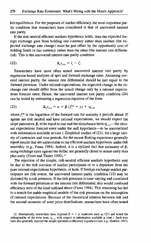
ket equilibrium. For the purposes of market efficiency, the most important par-ity condition that researchers have considered is that of uncovered interestrate parity.
If the risk-neutral efficient markets hypothesis holds, then the expected for-eign exchange gain from holding one currency rather than another (the ex-pected exchange rate change) must be just offset by the opportunity cost ofholding funds in this currency rather than the other (the interest rate differen-tial). This is the uncovered interest rate parity condition:
(22) \sl+k = i, - /;.
Researchers have most often tested uncovered interest rate parity byregression-based analyses of spot and forward exchange rates. Assuming cov-ered interest parity, the interest rate differential should be just equal to theforward premium. Under rational expectations, the expected change in the ex-change rate should differ from the actual change only by a rational expecta-tions forecast error. Hence, the uncovered interest rate parity condition (26)can be tested by estimating a regression equation of the form
(23) Akst+k = a + 3 ( / « - s,) + f]t+k,
where/* is the logarithm of the forward rate for maturity k periods ahead. Ifagents are risk neutral and have rational expectations, we should expect theslope parameter, (3, to be equal to one and the disturbance term r\l+k—the ratio-nal expectations forecast error under the null hypothesis—to be uncorrelatedwith information available at time t. Empirical studies of (23), for a large vari-ety of currencies and time periods, for the recent floating experience generallyreport results that are unfavorable to the efficient markets hypothesis under riskneutrality (e.g., Fama 1984). Indeed, it is a stylized fact that estimates of (3,using exchange rates against the dollar, are generally closer to minus unity thanplus unity (Froot and Thaler 1990).12
The rejection of the simple, risk-neutral efficient markets hypothesis maybe due to the risk aversion of market participants or to a departure from thepure rational expectations hypothesis, or both. If foreign exchange market par-ticipants are risk averse, the uncovered interest parity condition (22) may bedistorted by a risk premium. If the risk premium is time varying and correlatedwith the forward premium or the interest rate differential, this would confoundefficiency tests of the kind outlined above (Fama 1984). This reasoning has ledto a search for stable empirical models of the risk premium on the assumptionof rational expectations. Because of the theoretical relation between risk andthe second moments of asset price distributions, researchers have often tested
12. Alternatively, researchers have imposed 3 = 1 in equations such as (23) and tested theorthogonality of the error term, r\l+k, with respect to information available at time /. Such testshave also generally rejected the simple speculative efficiency hypothesis (see, e.g., Hodrick 1987).
276 Robert P. Flood and Mark P. Taylor
for a risk premium as a function of the variance of forecast errors or of ex-change rate movements (Frankel 1982; Domowitz and Hakkio 1985; Giovan-nini and Jorion 1989). In common with other empirical risk premium models,such as latent variables formulations (Hansen and Hodrick 1983), such modelshave generally met with mixed and somewhat limited success and have notbeen found to be robust when applied to different data sets and sample periods.In sum, it appears that, for credible degrees of risk aversion, empirical riskpremium models have so far been unable to explain to any significant degreethe variation in the excess return from forward market speculation.
An alternative explanation of the rejection of the simple efficient marketshypothesis is that there is a failure, in some sense, of the expectations compo-nent of the joint hypothesis. Examples in this group are the "peso problem"suggested by Kenneth Rogoff (1979), rational bubbles, learning about regimeshifts (Lewis 1989), or inefficient information processing (as suggested, e.g.,by John Bilson [1981]). The peso problem refers to the situation where agentsattach a small probability to a large change in the economic fundamentals,which does not occur in sample. This will tend to produce a skew in the distri-bution of forecast errors even if agents' expectations are rational and thus maygenerate apparent evidence of nonzero excess returns from forward specula-tion. In common with peso problems, the presence of rational bubbles mayalso show up as nonzero excess returns even when agents are risk neutral. Sim-ilarly, when agents are learning about their environment, they may be unablefully to exploit arbitrage opportunities that are apparent in the data ex post.A problem with admitting peso problems, bubbles, or learning into the classof explanations of the forward discount bias is that, as noted above, a verylarge number of econometric studies—encompassing an even larger rangeof exchange rates and sample periods—have found that the direction of biasis the same, that is, that the estimated uncovered interest rate parity slopeparameter, (3 in (23), is generally negative and closer to minus unity than plusunity.
A problem with much of the empirical work on the possible rationalizationsof the rejection of the simple, risk-neutral efficient markets hypothesis is that,in testing one leg of the joint hypothesis, researchers have typically assumedthat the other leg is true. For instance, the search for a stable empirical riskpremium model has generally been conditioned on the assumption of rationalexpectations. Thus, some researchers have employed survey data on exchangerate expectations to conduct tests of each component of the joint hypothesis(Froot and Frankel 1989). In general, the overall conclusion that emerges fromsurvey data studies appears to be that both risk aversion and departures fromrational expectations are responsible for rejection of the simple efficient mar-kets hypothesis.13
13. For surveys of the literature on foreign exchange risk premia, see Frankel (1988) andLewis (1994).
277 Exchange Rate Economics: What's Wrong with the Macro Approach?
8.3 What's Right with the Conventional Macro Approach?
In this section, we present some further empirical evidence on the relationbetween exchange rate movements and macroeconomic fundamentals by ex-amining the purchasing power parity and uncovered interest rate parity condi-tions, using panel data for twenty-two countries.14
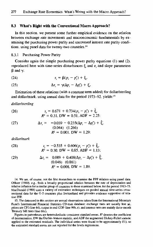
8.3.1 Purchasing Power Parity
Consider again the simple purchasing power parity equations (1) and (2),reproduced here with time-series disturbances £r and et and slope parametersP and y:
(24) s, = P(ft - pt) + i,
(25) As, = y(Apt - Atf) + £.
Estimation of these relations (with a constant term added) for dollar/sterlingand dollar/mark, using annual data for the period 1973-92, yields:15
dollar/sterling
(26) s, = 0.671 + 0.734(/?, - p*t) + %,R2 = 0.31, DW = 0.51, ADF = 2.25;
(27) As, = -0.039 - 0.235(Ap, - Ap*) + £,(0.044) (1.266)
R2 = 0.001, DW = 1.29;
dollar/mark
(28) st = -0.535 + 0.606(/?, - p*t) + |,,R2 = 0.30, DW = 0.85, ADF =1.13;
(29) As, = 0.009 + 0.408(Apr - Ap*t) + £,(0.046) (0.861)R2 = 0.008, DW = 1.89.
14. We are, of course, not the first researchers to examine the PPP relation using panel data.Officer (1980), e.g., finds a broadly proportional relation between the rate of depreciation andrelative inflation for a similar group of countries to those examined below, for the period 1913-75.MacDonald (1988) uses a variety of estimation techniques on pooled annual time-series cross-sectional data for the G-5 countries plus Switzerland and provides evidence supportive of rela-tive PPP.
15. The data used in this section are annual observations taken from the International MonetaryFund's International Financial Statistics CD-rom database: exchange rates are usually line ae,prices are CPI (line 64), output is real GDP (line 99b. r), and interest rates are mainly three-monthTreasury bill rates (line 60c).
Figures in parentheses are heteroskedastic-consistent standard errors, fl2 denotes the coefficientof determination, DW the Durbin-Watson statistic, and ADF the augmented Dickey-Fuller statisticapplied to the estimated residuals. The individual series were found to be approximately 1(1), sothe estimated standard errors are not reported for the levels regressions.

278 Robert P. Flood and Mark P. Taylor
-30 -20 -10 0 10 20 30 40 50 60 70
Fig. 8.4 Scatter plot of annual exchange rate change against annual inflationdifferential
These equations are typical of single-equation results reported in the litera-ture for the recent floating-rate period: there is no apparent sign of cointegra-tion of the exchange rate and relative prices, and relative inflation explains lessthan 1 percent of the time-series variation in the nominal exchange rate.
In figure 8.4, we have plotted the annual exchange rate change against theannual inflation differential for twenty-one industrialized countries against theUnited States for the period 1973-92.16 This scatter plot is vaguely suggestiveof a positive linear relation between the rate of depreciation and the inflationdifferential, especially for large inflation differentials.
In figure 8.5, we also plot the annual rate of depreciation against the UnitedStates, but this time using five-year averages (four for each country, corre-sponding to the periods 1973-77, 1978-82, and 1983-87, and 1988-92). Fig-ure 8.5 appears to reveal a stronger medium-term relation between the ex-change rate and relative inflation, in the sense that the scatter is much closer tothe forty-five-degree line, albeit with one or two outliers. When the data areaveraged over periods of ten or twenty years (figs. 8.6 and 8.7, respectively),the proportionality between average relative inflation and average depreciationbecomes even more marked, as the scatter more or less collapses onto theforty-five-degree ray.
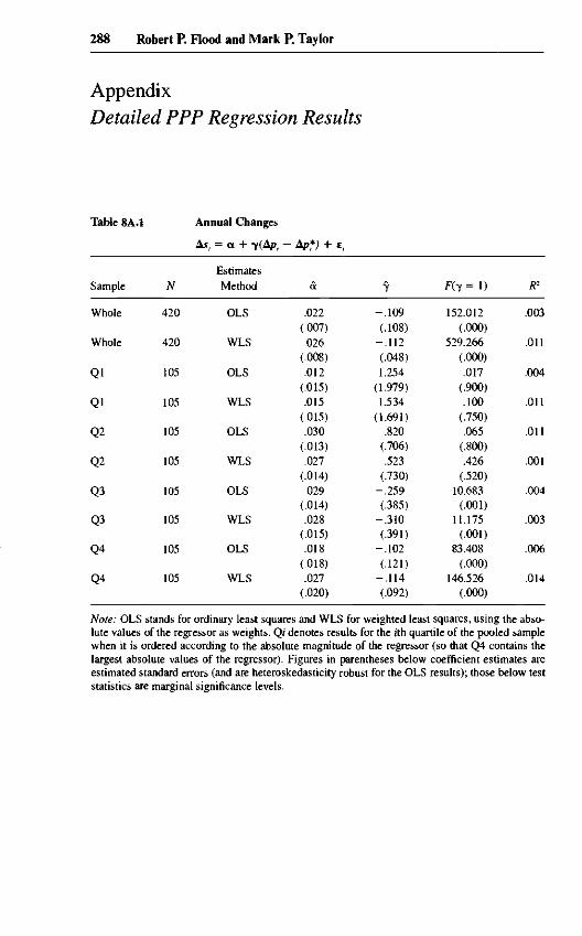
These visual impressions are largely confirmed by regression analysis, thefull results of which are given in the appendix. By simply pooling the twentyyears of data on annual changes, for example, we obtained the followingpooled estimate:
16. The countries besides the United States included in the sample are Australia, Austria, Bel-gium, Canada, Denmark, Finland, France, Germany, Greece, Iceland, Ireland, Italy, Japan, theNetherlands, New Zealand, Norway, Portugal, Spain, Sweden, Switzerland, and the United King-dom. All data were taken from the IFS database.

-30 -20 -10 0 10 20 30 40 50 60 70 80
Fig. 8.5 Scatter plot of five-year average exchange rate change against five-yearaverage inflation differential
-30 -20 -10 0 10 20 30 40 50 60 70 80
Fig. 8.6 Scatter plot of ten-year average exchange rate change against ten-yearaverage inflation differential
-30 -20 -10 0 10 20 30 40 50 60 70 80
Fig. 8.7 Scatter plot of twenty-year average exchange rate change againsttwenty-year average inflation differential
280 Robert P. Flood and Mark P. Taylor
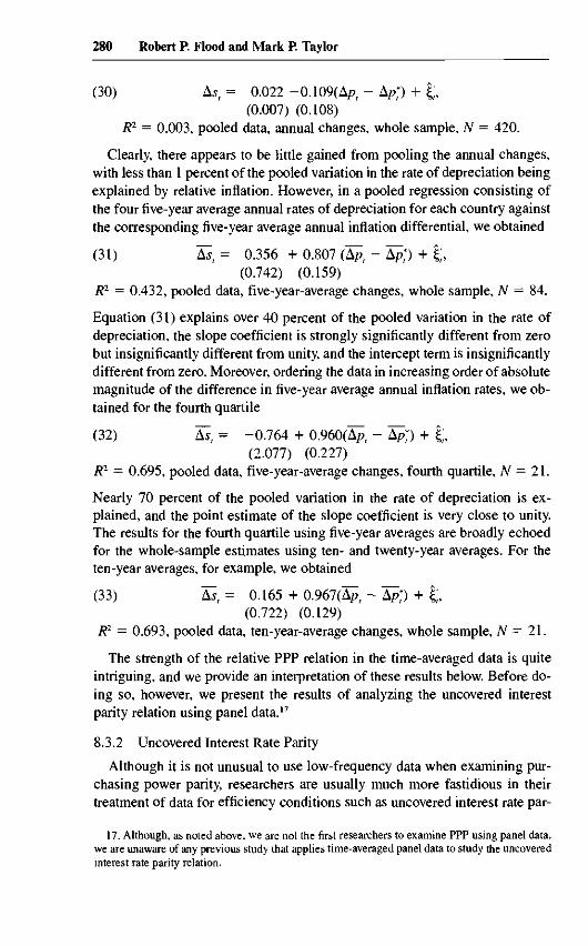
(30) As, = 0.022 -0.109(Ap, - A/?,*) + £,(0.007) (0.108)
R2 = 0.003, pooled data, annual changes, whole sample, N = 420.
Clearly, there appears to be little gained from pooling the annual changes,with less than 1 percent of the pooled variation in the rate of depreciation beingexplained by relative inflation. However, in a pooled regression consisting ofthe four five-year average annual rates of depreciation for each country againstthe corresponding five-year average annual inflation differential, we obtained
(31) As, = 0.356 + 0.807 (Ap, - ApJ) + £,(0.742) (0.159)
R2 — 0.432, pooled data, five-year-average changes, whole sample, N = 84.
Equation (31) explains over 40 percent of the pooled variation in the rate ofdepreciation, the slope coefficient is strongly significantly different from zerobut insignificantly different from unity, and the intercept term is insignificantlydifferent from zero. Moreover, ordering the data in increasing order of absolutemagnitude of the difference in five-year average annual inflation rates, we ob-tained for the fourth quartile
(32) As, - -0.764 + 0.960(Ap", - Atf) + £,(2.077) (0.227)
R2 — 0.695, pooled data, five-year-average changes, fourth quartile, N — 21.
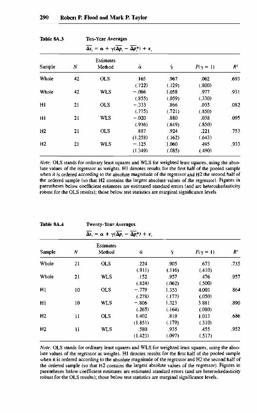
Nearly 70 percent of the pooled variation in the rate of depreciation is ex-plained, and the point estimate of the slope coefficient is very close to unity.The results for the fourth quartile using five-year averages are broadly echoedfor the whole-sample estimates using ten- and twenty-year averages. For theten-year averages, for example, we obtained
(33) As, = 0.165 + 0.967(Kpt ~ Apr*) + £,(0.722) (0.129)
R2 = 0.693, pooled data, ten-year-average changes, whole sample, N = 21.
The strength of the relative PPP relation in the time-averaged data is quiteintriguing, and we provide an interpretation of these results below. Before do-ing so, however, we present the results of analyzing the uncovered interestparity relation using panel data.17
8.3.2 Uncovered Interest Rate Parity
Although it is not unusual to use low-frequency data when examining pur-chasing power parity, researchers are usually much more fastidious in theirtreatment of data for efficiency conditions such as uncovered interest rate par-
17. Although, as noted above, we are not the first researchers to examine PPP using panel data,we are unaware of any previous study that applies time-averaged panel data to study the uncoveredinterest rate parity relation.
281 Exchange Rate Economics: What's Wrong with the Macro Approach?
ity and covered interest rate parity (see, e.g., Hodrick 1987; Taylor 1988,1989). This is for good reasons—namely, that tiny mismatches or imperfec-tions in the data may be mistaken for arbitrage opportunities that, althoughsmall in size, would nevertheless be highly profitable for a foreign exchangemarket participant moving around very large sums of money. In the presentcontext, however, we are concerned with looking at uncovered interest rateparity in very broad terms, to see whether interest differentials have any rela-tion with exchange rate movements.18 Clearly, our results should be taken asindicative only.
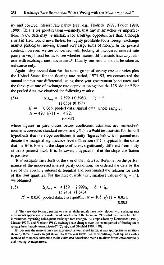
Again using annual data for the same group of twenty-one countries plusthe United States for the floating-rate period, 1973-92, we constructed theannual interest rate differential, using three-year government bond rates, andthe three-year rate of exchange rate depreciation against the U.S. dollar.19 Forthe pooled data, we obtained the following results:
(34) A3s,+3 = 2.599 +0.596(*, - 0 + r\t,(1.656) (0.195)
R2 = 0.066, pooled data, annual data, whole sample,N = 420, x2(l) = 4.72,
(0.038)
where figures in parentheses below coefficient estimates are method-of-moments corrected standard errors, and x2(l) is a Wald test statistic for the nullhypothesis that the slope coefficient is unity (figures below it in parenthesesdenote the marginal significance level). Equation (34) is typical in the sensethat the R2 is low and the slope coefficient significantly different from unityat the 5 percent level. It is, however, untypical in that the slope coefficientis positive.
To investigate the effects of the size of the interest differential on the perfor-mance of the uncovered interest parity condition, we ordered the data by thesize of the absolute interest differential and reestimated the relation for eachof the four quartiles. For the first quartile (i.e., smallest values of \it - i*\),we obtained
(35) A35,+3 = 4.159 - 2.9990; - O + \ ,(3.243) (1.343)
R2 = 0.036, pooled data, first quartile, N = 105, X2U) = 8.851,
(0.003)
18. The view that forward premia or interest differentials have little relation with exchange ratemovements appears to be a widespread conclusion of the literature: "Forward premia contain littleinformation regarding subsequent exchange rate changes. As emphasized by Dornbusch (1980),Mussa (1979), and Frenkel (1981), exchange rate changes over the recent period of floating seemto have been largely unanticipated" (Cumby and Obstfeld 1984, 139).
19. Because the interest rates are expressed in annualized terms, it was appropriate to multiplythem by three in order to put them into three-year terms. We used ordinary least squares with amethod-of-moments correction to the estimated covariance matrix to allow for heteroskedasticityand moving-average errors.

282 Robert P. Flood and Mark P. Taylor
which exhibits the characteristic negative slope coefficient and a lower R2.For the second quartile, the result was
(36) A35f+3 = 5.208 - 0.798(ir - 0 + U(1.732) (0.475)
R2 = 0.024, pooled data, second quartile, N = 105, x2(l) = 14.345,(0.000)
which shows a very typical slope coefficient estimate that is closer to minusunity than plus unity and an even smaller R2.
For the third quartile, we obtained
(37) A35f+3= -1 .405+ 0.609 (i, - O + fj,,(2.841) (0.329)
R2 = 0.046, pooled data, third quartile, N = 105, x2(l) = 1-409,(0.235)
while, for the fourth quartile (i.e., the largest values of \ir — i*\), the resultingestimate was
(38) A35f+3 = 11.121 + 0.5200; - O + fj,(7.460) (0.273)
R2 = 0.079, pooled data, fourth quartile, N = 105, x2(l) = 3.087.(0.079)
It is interesting to note that, for the third and fourth quartiles, the slope coef-ficient is insignificantly different from unity at the 5 percent level. However,although there is some improvement in the goodness of fit, the /?2's are stillquite low, and the slope coefficients are not in fact significantly different fromzero at the 5 percent level.
As in the analysis of PPP, the next step was to average the data temporally.Using pooled five-year averages for the data for the whole sample, we obtainedthe following estimate:
(39) A3s,+3 = 0.632 + 0.751(ir - O + f),,(2.020) (0.171)
R2 = 0.190, pooled data, five-year averages, whole sample,N = 84, x2(l) = 2.124.
(0.145)
Equation (39) is quite impressive in the sense that the goodness of fit has risendramatically from the unaveraged cases—by a factor of twenty-five or more.Moreover, the slope coefficient is now strongly significantly different fromzero and insignificantly different from zero at the 5 percent level. These effectswith respect to the goodness of fit and the slope coefficient are even more

283 Exchange Rate Economics: What's Wrong with the Macro Approach?
marked when we consider the results of running the same regressions usingdata that have been time averaged over ten or twenty years:
(40) A35r+3 = 0.706 + 1.075(if - ij) + fjf,(1.942) (0.111)
R2 = 0.400, pooled data, ten-year averages, whole sample,N = 42, x2(l) = 0.461;
(0.497)
(41) A35,+3 = -2.721 + 1.481(1, - O + %(1.556) (0.293)
R2 - 0.772, pooled data, twenty-year averages, whole sample,N = 42, x2(l) = 2.697.
(0.100)
Given the plethora of results on uncovered interest rate parity that havefound little or no empirical connection between interest rates and the exchangerate or, if anything, have found negative covariation between the interest differ-ential or forward premium and the rate of depreciation, these results are verystriking and quite intriguing. Moreover, as we noted above, we have used aready-made data set from the IFS (International Financial Statistics, Interna-tional Monetary Fund) and have not spent a great deal of time worrying aboutaligning maturity dates, checking that the instruments are identical in all rele-vant respects across countries, and so on. These shortcomings in the data setwould be most relevant if we did not find evidence of uncovered interest rateparity in the averaged data; as it is, they serve only to underscore the strengthof the relation that we appear to be unearthing.
8.3.3 Interpretation
In this section, we have shown that very simple macro fundamentals—rela-tive inflation or relative interest rates—have poor explanatory power with re-spect to variations in exchange rate movements even over the one-year horizon.Taking five-, ten-, and twenty-year averages, however, we found that a strongproportionality between average exchange rate depreciation and average move-ments in the fundamentals begins to emerge. The analysis is thus indicative ofsomething that Rick and lisa knew long ago: the fundamental things apply astime goes by. Moreover, the analysis also suggests that the variation of devia-tions from the fundamentals appears to be inversely related to the size of themovements in the underlying fundamentals.
Our interpretation of these results is that, while the nominal exchange rateis extremely hard to distinguish from a random walk even at the one-year hori-zon, a simple macro fundamentals-based model outperforms the random walkat horizons of five years or longer. To see this clearly, note that the n-yearaverage annual change in the exchange rate is defined as

284 Robert P. Flood and Mark P. Taylor
(43) (l/n)j>>s,+1- = d/n)(st+n - s,).i=0
Thus, finding that the n-year average exchange rate change is explained bymacro fundamentals is equivalent to finding that the «-year-ahead random-walk forecast is beaten in sample by a simple macro fundamentals model.
The results also tell us something about the nature of deviations from thefundamentals. The change in the exchange rate can be defined as the sum of acomponent that is explained by movements in the macro fundamentals (suchas relative inflation or relative nominal interest rates, or whatever macro vari-ables that, in turn, determine them), Ft, and a component that is unexplainedby the macro fundamentals, U,:
(43) As, - F, + Ur
When As, is averaged over periods of five years or more, the estimated slopecoefficient from a regression of As, onto Ft tends toward unity, and the R2 risesdramatically, a result that holds for both the PPP and the UIP (uncovered inter-est rate parity) analyses. This implies that the variance of the movement in theexchange rate unexplained by the macro fundamentals declines dramaticallyover periods of five years or more, which must mean that the year-by-year time-series errors cancel out approximately:
n
(44) (l/n)X u,+i * °' forn > 5 years.i = 0
Thus, there appears to be little effect from omitting Ut from the regressionsusing averaged data. However, the fact that the estimated slope coefficient inthe regressions using annual, unaveraged data is quite different from the esti-mates obtained using the averaged data suggests that the unexplained compo-nent is correlated with the component of the change explained by the macrofundamentals at the annual level:
(45) Corr(F,, U) # 0.
One interpretation of our results is that averaging Ut provides a filter thatvastly reduces the variance of the disturbance term and that much of this reduc-tion is in terms of reduced covariation of the residual with the fundamental.This covariance, of course, would also be reduced if we had truly exogenousfundamentals or instruments for the fundamentals.
Thus, our analysis suggests the following. First, short-run deviations of theexchange rate, from the path consistent with the macro fundamentals alone,are responsible for the greater proportion of the short-run variation in nominalexchange rates. Second, these deviations apparently cancel out over periods offive years or more. Third, and perhaps most puzzling, the deviations appear tobe correlated with the fundamentals themselves in the annual data.

285 Exchange Rate Economics: What's Wrong with the Macro Approach?
8.4 Conclusion: What's Wrong with the ConventionalMacro Approach?
The empirical work summarized in sections 8.1 and 8.2 suggests that, forindustrial countries during "normal times" (i.e., when they are not experienc-ing economic pathologies such as a hyperinflation), conventional macro funda-mental models of exchange rate behavior are incapable of explaining thegreater proportion of the variation in nominal exchange rate movements. It isapparent that there are important influences, not on the list of standard macrofundamentals, that affect short-run exchange rate behavior, and standardmacro-based models perform poorly when subjected to standard time-serieseconometric testing—typically providing poor in-sample fits and miserablepostsample predictive performance. Hence, there seems to be little profes-sional disagreement with the view that, as a guide to the short-run behavior ofthe major exchange rates, exchange rate models based on macro fundamentalshave largely failed.
The macro-based models have, to some extent, been rehabilitated in studiesthat have used cointegration or error-correction-type models to forecast theexchange rate. These studies, however, in common with recent cointegrationstudies on exchange rates and purchasing power parity, provide evidence forthe view that it is the longer-run or low-frequency movements in exchangerates that are correlated with the traditional macro fundamentals, while theshorter run movements are poorly understood or, to use the applied researcher'seuphemism, "noisy."
Some generic evidence on the relevance of economic fundamentals forshort-run exchange rate behavior is provided in a recent study by Flood andRose (1993). Observing the increased volatility of exchange rates under float-ing as opposed to fixed exchange rate regimes, these authors argue that anytentatively adequate exchange rate model should have fundamentals that arealso much more volatile during floating-rate regimes. In fact, they find littleshift in the volatility of economic fundamentals suggested by flexible-price orsticky-price monetary models across different nominal exchange rate regimesfor a number of OECD exchange rates. Similar evidence is reported by Baxterand Stockman (1989). More generally, a number of studies have noted that,under the recent float, nominal exchange rates have shown much greater vari-ability than important macroeconomic fundamentals such as price levels andreal incomes (e.g., Dornbusch and Frankel 1988; Frankel and Froot 1990; Mar-ston 1989).20 Again, this suggests that there are speculative forces at work in
20. Some analyses suggest that exchange rate volatility can change dramatically across regimeseven though the volatility of the macro fundamentals does not. This point was crucial, e.g., in theDornbusch (1976) overshooting model and in the Krugman (1991) target zone model. In boththese models, and in rational expectations models in general, the Lucas critique applies, and theform of the reduced-form relation between the exchange rate and the fundamentals is not invariant

286 Robert P. Flood and Mark P. Taylor
the foreign exchange market that are not reflected in the usual menu of macro-economic fundamentals: given the exhaustive interrogation of the macro fun-damentals in this respect over the last twenty years, it would seem that ourunderstanding of the short-run behavior of exchange rates is unlikely to befurther enhanced by further examination of the macro fundamentals. And it isin this context that new work on the microstructure of the foreign exchangemarket seems both warranted and promising.
The results of the research program into the speculative efficiency of theforeign exchange market also have important implications for the new researchprogram into the microstructure of foreign exchange markets as well as themore conventional, macro-based approach. In particular, the rejection of thesimple speculative efficiency hypothesis as applied to the foreign exchangemarket and the stylized empirical fact of a negative covariation between therate of depreciation and the forward premium challenges conventional, macro-based approaches to the foreign exchange market since it suggests that onecannot take for granted many of the efficiency conditions that are typicallysubsumed in macro-based exchange rate models. Even under the assumptionof risk aversion alongside that of rational expectations, the stylized fact of theso-called negative discount bias is very hard to explain (Fama 1984). More-over, the evidence, from studies employing survey data, that foreign exchangemarket participants are neither risk averse nor conform to the rational expecta-tions hypothesis suggests that the heterogeneity of agents' expectations acrossthe foreign exchange market—itself highlighted in some recent survey datastudies—may itself be an important feature determining short-run exchangerate behavior. The processes by which information is obtained and dissemin-ated throughout markets is not amenable to analysis within a standard macroapproach but is clearly of major importance given heterogeneity of agents'expectations and information sets (see, e.g., Lyons 1995). Information pro-cessing may also be at the root of the contagion in volatility across foreignexchange markets that has been documented.21 Moreover, the finding that ahigh proportion of foreign exchange market participants deliberately use ana-lytic techniques that ignore macro fundamentals (i.e., "technical" or "chartist"analysis), especially over shorter horizons (Taylor and Allen 1992), under-scores the importance of allowing for the interaction of diverse forces in theshort-run determination of exchange rates (Goodhart 1988; Frankel and Froot1990).
to the policy regime. To circumvent this well-known critique as well as the possibility that thepresence of exchange rate bubbles may be regime dependent, Flood and Rose (1993) studied ex-change rate and fundamentals volatility in structural equations rather than reduced-form expres-sions so that their conclusions are close to immune to the Lucas critique and bubbles issue. Wesay "close to immune" because it could be that exchange rate policy change results in structuralcoefficient drift, but this would be a thin reed on which to base exchange rate models.
21. So-called meteor showers (Engle, Ito, and Lin 1990).
287 Exchange Rate Economics: What's Wrong with the Macro Approach?
The additional empirical results reported in this paper underscore the viewthat empirical work on macro-based exchange rage models has been hamperedby "contamination" of the data with a high degree of short-run noise. Industrialcountries are different from each other, but the differences in exchangerate fundamentals change very slowly through time, while exchange ratetime series show comparatively huge variation. To investigate this question,we work with a panel of data on twenty-two industrialized countries (in-cluding the United States) during the recent floating exchange rate era. In ourinvestigation, we suppress noisy time-series variation in a series of steps. Wefirst study two very simple exchange rate relations, relative purchasing powerparity and uncovered interest rate parity, with annual data, then with five-year averaged, ten-year averaged, and, finally, twenty-year averaged data.Formally, as we temporally average the data, we also temporally average thetime-series disturbances until, eventually, they disappear, leaving us with across-sectional model apparently purged of temporal noise. We find that thesimple fundamentals models work extremely well in the pure cross section,with inflation or interest rate differentials explaining a very high proportionof the cross-sectional variation in exchange rate movements. We have,therefore, provided some additional evidence that the macro fundamentalsshould not be dismissed entirely. It is clear that the macro fundamentalsin an important sense "set the parameters" within which exchange ratesmove but that these parameters are very broad indeed over the short run.Developing microstructural models of short-run exchange rate movementswithin these wide parameters is the challenge that researchers in this fieldnow face.
288 Robert P. Flood and Mark P. Taylor
AppendixDetailed PPP Regression Results
Table 8A.1
Sample
Whole
Whole
Ql
Ql
Q2
Q2
Q3
Q3
Q4
Q4
N
420
420
105
105
105
105
105
105
105
105
Annual Changes
As, = a + "y(Ap,
EstimatesMethod
OLS
WLS
OLS
WLS
OLS
WLS
OLS
WLS
OLS
WLS
- bp?) + e,
a
.022(.007).026
(.008).012
(.015).015
(.015).030
(.013).027
(.014).029
(.014).028
(.015).018
(.018).027
(.020)
y
-.109(.108)
-.112(.048)1.254
(1.979)1.534
(1.691).820
(.706).523
(.730)-.259(.385)
-.310(.391)
-.102(.121)
-.114(.092)
F(y = 1)
152.012(.000)
529.266(.000).017
(.900).100
(.750).065
(.800).426
(.520)10.683
(.001)11.175
(.001)83.408
(.000)146.526
(.000)
R2
.003
.011
.004
.011
.011
.001
.004
.003
.006
.014
Note: OLS stands for ordinary least squares and WLS for weighted least squares, using the abso-lute values of the regressor as weights. Oj denotes results for the ith quartile of the pooled samplewhen it is ordered according to the absolute magnitude of the regressor (so that Q4 contains thelargest absolute values of the regressor). Figures in parentheses below coefficient estimates areestimated standard errors (and are heteroskedasticity robust for the OLS results); those below teststatistics are marginal significance levels.

289 Exchange Rate Economics: What's Wrong with the Macro Approach?
Table 8A.2
Sample
Whole
Whole
Ql
Ql
Q2
Q2
Q3
Q3
Q4
Q4
N
84
84
21
21
21
21
21
21
21
21
Five-Year Averages
As, = a + Y(A/>, —
EstimatesMethod
OLS
WLS
OLS
WLS
OLS
WLS
OLS
WLS
OLS
WLS
Ap?) + e,
a
.356(.742)
-.108(.984).592
(1.109)-.474(1.165)-.344(1.264)-.523(1.344)
.510(1.287)1.221
(1.327)-.764(2.077)
-2.050(2.684)
P
.807(.159)
-.955(.064)1.927
(1.539)1.908
(1.298).202
(.751).327
(.769)-.223(.364)
-.202(.344).960
(.227)1.059(.143)
F(y = 1)
1.490(.220).463
(.490).362
(.540).489
(.490)1.128(.290).767
(.390)11.262
(.001)12.188
(.002).031
(.860).171
(.680)
R2
.432
.812
.065
.100
.004
.012
.019
.039
.695
.837
Note: OLS stands for ordinary least squares and WLS for weighted least squares, using the abso-lute values of the regressor as weights. Qi denotes results for the ith quartile of the pooled samplewhen it is ordered according to the absolute magnitude of the regressor (so that Q4 contains thelargest absolute values of the regressor). Figures in parentheses below coefficient estimates areestimated standard errors (and are heteroskedasticity robust for the OLS results); those below teststatistics are marginal significance levels.
290 Robert P. Flood and Mark P. Taylor
Table 8A.3
Sample
Whole
Whole
HI
HI
H2
H2
N
42
42
21
21
21
21
Ten-Year Averages
As, = a + 7(Ap, —
EstimatesMethod
OLS
WLS
OLS
WLS
OLS
WLS
Ap*) + E,
a
.165(.722)
-.086(.855)
-.333(-775)
-.020(.916).887
(1.258)-.125(1.349)
7
.967(.129)1.058(.059).866
(.721).880
(.619).924
(.162)1.060(.085)
F(y = 1)
.062(.800).977
(.330).035
(.850).038
(.850).221
(.643).495
(.490)
R2
.693
.931
.082
.095
.753
.933
Note: OLS stands for ordinary least squares and WLS for weighted least squares, using the abso-lute values of the regressor as weights. HI denotes results for the first half of the pooled samplewhen it is ordered according to the absolute magnitude of the regressor and H2 the second half ofthe ordered sample (so that H2 contains the largest absolute values of the regressor). Figures inparentheses below coefficient estimates are estimated standard errors (and are heteroskedasticityrobust for the OLS results); those below test statistics are marginal significance levels.
Table 8A.4
Sample
Whole
Whole
HI
HI
H2
H2
N
21
21
10
10
11
11
Twenty-Year Averages
As, = a + v(Ap,
EstimatesMethod
OLS
WLS
OLS
WLS
OLS
WLS
- Ap,*; + e,
&
.224(.911).152
(.824)-.779(.278)
-.806(.265)1.402
(1.851).580
(1.423)
7
.905(.116).957
(.062)1.353(.177)1.323(.164).819
(.179).935
(.097)
F(y = 1)
.673(.410).476
(.500)4.003(.050)3.881(.080)1.013(.310).455
(.517)
R2
.735
.957
.864
.890
.686
.952
Note: OLS stands for ordinary least squares and WLS for weighted least squares, using the abso-lute values of the regressor as weights. HI denotes results for the first half of the pooled samplewhen it is ordered according to the absolute magnitude of the regressor and H2 the second half ofthe ordered sample (so that H2 contains the largest absolute values of the regressor). Figures inparentheses below coefficient estimates are estimated standard errors (and are heteroskedasticityrobust for the OLS results); those below test statistics are marginal significance levels.

291 Exchange Rate Economics: What's Wrong with the Macro Approach?
References
Adler, Michael, and Bruce Lehmann. 1983. Deviations from purchasing power parityin the long run. Journal of Finance 38, no. 4:1471-78.
Backus, David K. 1984. Empirical models of the exchange rate: Separating the wheatfrom the chaff. Canadian Journal of Economics 17:824-46.
Baxter, Marianne, and Alan C. Stockman. 1989. Business cycles and the exchange rateregime: Some international evidence. Journal of Monetary Economics 23, no.3:377-400.
Bilson, John E O. 1978. Rational expectations and the exchange rate. In The economicsof exchange rates, ed. Jacob A. Frenkel and Harry G. Johnson. Reading, Mass.:Addison-Wesley.
. 1981. The speculative efficiency hypothesis. Journal of Business 54:435-51.Branson, William H., Hannu Halttunen, and Paul R. Masson. 1977. Exchange rates in
the short run: The dollar-deutschemark rate. European Economic Review 10, no.4:303-24.
Branson, William H., and Dale W. Henderson. 1985. The specification and influence ofasset markets. In Handbook of international economics, ed. Ronald W. Jones andPeter B. Kenen. Amsterdam: North-Holland.
Cheung, Yin-Wong, and Kon S. Lai. 1993. Long-run purchasing power parity duringthe recent float. Journal of International Economics 34, no. 1:181-92.
Cumby, Robert E., and Maurice Obstfeld. 1984. International interest rate and pricelevel linkages under flexible exchange rates: A review of recent evidence. In Ex-change rate theory and practice, ed. John F. O. Bilson and Richard C. Marston. Chi-cago: University of Chicago Press.
Dominguez, Kathryn M., and Jeffrey A. Frankel. 1993. Does foreign exchange inter-vention matter? The portfolio effect. American Economic Review 83, no. 4:1356-69.
Domowitz, Ian, and Craig Hakkio. 1985. Conditional variance and the risk premium inthe foreign exchange market. Journal of International Economics 19, no. 3:47-66.
Dornbusch, Rudiger. 1976. Expectations and exchange rate dynamics. Journal of Politi-cal Economy 84, no. 6:1161-76.
. 1980. Exchange rate economics: Where do we stand? Brookings Papers onEconomic Activity 143-85.
Dornbusch, Rudiger, and Jeffrey Frankel. 1988. The flexible exchange rate system: Ex-perience and alternatives. In International Trade and Finance in a Polycentric World,ed. Silvio Borner. New York: St. Martin's Press.
Engle, Robert E, Takatoshi Ito, and Wen-Ling Lin. 1990. Meteor showers or heatwaves? Heteroskedastic intra-daily volatility in the foreign exchange market. Econo-metrica 58, no. 3:525-42.
Fama, Eugene F. 1984. Forward and spot exchange rates. Journal of Monetary Econom-ics 14, no. 3:319-38.
Flood, Robert P. 1981. Explanations of exchange rate volatility and other empiricalregularities in some popular models of the foreign exchange market. Carnegie-Rochester Conference Series on Public Policy 15 (Autumn): 219-49.
Flood, Robert P., and Andrew K. Rose. 1993. Fixing exchange rates: A virtual quest forfundamentals. Discussion Paper no. 838. London: Centre for Economic PolicyResearch.
Frankel, Jeffrey A. 1979. On the mark: A theory of floating exchange rates based onreal interest differentials. American Economic Review 69:610-22.
. 1982. In search of the exchange risk premium: A six-currency test assumingmean-variance optimization. Journal of International Money and Finance 1, no.3:255-74.
292 Robert P. Flood and Mark P. Taylor
. 1988. Recent estimates of time-variation in the conditional variance and in theexchange risk premium. Journal of International Money and Finance 7, no.1:115-25.
-. 1990. Zen and the art of modern macroeconomics: The search for perfect noth-ingness. In Monetary policy for a volatile global economy, ed. William Haraf andThomas Willett. Washington, D.C.: American Enterprise Institute.
-. 1993. Monetary and portfolio balance models of the determination of exchangerates. In On exchange rates. Cambridge, Mass.: MIT Press.
Frankel, Jeffrey A., and Kenneth A. Froot. 1990. Chartists, fundamentalists and thedemand for dollars. In Private behaviour and government policy in interdependenteconomies, ed. Anthony S. Courakis and Mark P. Taylor. Oxford: Oxford UniversityPress.
Frankel, Jeffrey A., and Andrew K. Rose. 1994. An empirical characterization of nomi-nal exchange rates. Department of Economics, University of California, Berkeley.Mimeo.
Frenkel, Jacob A. 1976. A monetary approach to the exchange rate: Doctrinal aspectsand empirical evidence. Scandinavian Journal of Economics 78, no. 1:200-224.
. 1981. Flexible exchange rates, prices and the role of "news." Journal of Politi-cal Economy 89:665-705.
Frenkel, Jacob A., and Harry G. Johnson, eds. 1978. The economics of exchange rates.Reading, Mass.: Addison-Wesley.
Friedman, Milton. 1953. The case for flexible exchange rates. In Essays in positiveeconomics, ed. Milton Friedman. Chicago: University of Chicago Press.
Froot, Kenneth A., and Jeffrey A. Frankel. 1989. Forward discount bias: Is it an ex-change risk premium? Quarterly Journal of Economics 104, no. 1:139-61.
Froot, Kenneth A., and Richard H. Thaler. 1990. Anomalies: Foreign exchange. Journalof Economic Perspectives 4, no. 2:179-92.
Giovannini, Alberto, and Philippe Jorion. 1989. The time variation of risk and return inthe foreign exchange and stock markets. Journal of Finance 44, no. 2:307-25.
Goodhart, Charles A. E. 1988. The foreign exchange market: A random walk with adragging anchor. Economica 55, no. 4:437-60.
Hansen, Lars P., and Robert J. Hodrick. 1983. Risk averse speculation in the forwardforeign exchange market: An econometric analysis of linear models. In Exchangerates and international macroeconomics, ed. Jacob A. Frenkel. Chicago: Universityof Chicago Press.
Hodrick, Robert J. 1987. The empirical evidence on the efficiency of forward andfutures foreign exchange markets. London: Harwood.
Hooper, Peter, and John Morton. 1982. Fluctuations in the dollar: A model of nominaland real exchange rate determination. Journal of International Money and Financel,no. 1:39-56.
Krugman, Paul R. 1991. Target zones and exchange rate dynamics. Quarterly Journalof Economics 106, no. 3:669-82.
Lewis, Karen K. 1988. Testing and portfolio balance model: A multilateral approach.Journal of International Economics 24:133-50.
. 1989. Changing beliefs and systematic rational forecast errors with evidencefrom foreign exchange. American Economic Review 79, no. 4:621-36.
-. 1994. International financial markets. Wharton School, University of Pennsyl-vania. Mimeo.
Lothian, James R., and Mark P. Taylor. 1994. Real exchange rate behavior: The recentfloat from the perspective of the past two centuries. Washington, D.C.: InternationalMonetary Fund.
Lucas, Robert E. 1982. Interest rates and currency prices in a two-country world. Jour-nal of Monetary Economics 10, no. 4:335-59.

293 Exchange Rate Economics: What's Wrong with the Macro Approach?
Lyons, Richard K. 1995. Tests of microstructural hypotheses in the foreign exchangemarket. Journal of Financial Economics 39:321-51.
MacDonald, Ronald. 1988. Purchasing power parity: Some "long-run" evidence fromthe recent float. Economist 136, no. 2:239-51.
MacDonald, Ronald, and Mark P. Taylor. 1992. Exchange rate economics: A survey.International Monetary Fund Staff Papers 39, no. 1:1-57.
. 1993. The monetary approach to the exchange rate: Rational expectations,long-run equilibrium, and forecasting. International Monetary Fund Staff Papers 40,no. 1:89-107.
1994. The Monetary Model of the exchange rate: Long-run relationships,short-run dynamics, and how to beat a random walk. Journal of International Moneyand Finance.
Mark, Nelson C. 1990. Real and nominal exchange rates in the long run. Journal ofInternational Economics 28, no. 1:115-36.
. 1992. Exchange rates and fundamentals: Evidence on long-horizon predict-ability and overshooting. Working paper. Ohio State University, August.
Marston, Richard C. 1989. Real and nominal exchange rate variability. Empirica 16,no. 2:147-60.
McNown, Robert, and Myles Wallace. 1989. National price levels, purchasing powerparity and cointegration: A test of four high-inflation economies. Journal of Interna-tional Money and Finance 8, no. 4:533-45.
Meese, Richard A., and Kenneth Rogoff. 1983a. Empirical exchange rate models of theseventies: Do they fit out of sample. Journal of International Economics 14, no.2:3-24.
. 1983b. The out-of-sample failure of empirical exchange rate models: Samplingerror or misspecification? In Exchange rates and international macroeconomics, ed.Jacob A. Frenkel. Chicago: University of Chicago Press.
-. 1988. Was it real? The exchange rate-interest differential relationship over themodern floating-rate period. Journal of Finance 43, no. 4:933-48.
Mussa, Michael. 1979. Empirical regularities in the behavior of exchange rates andtheories of the foreign exchange market. Carnegie-Rochester Conference Series onPublic Policy 11:9-57'.
. 1986. Nominal exchange rate regimes and the behavior of real exchange rates:Evidence and implications. Carnegie-Rochester Conference Series on Public Policy25:117-213.
Officer, Lawrence H. 1980. Effective exchange rates and price ratios over the long-run:A test of the purchasing power parity theory. Canadian Journal of Economics8:206-30.
Rogoff, Kenneth. 1979. Expectations and exchange rate volatility. Ph.D. diss., Massa-chusetts Institute of Technology.
. 1984. On the effects of sterilized intervention: An analysis of weekly data.Journal of Monetary Economics 14:133-50.
Stockman, Alan C. 1980. A theory of exchange rate determination. Journal of PoliticalEconomy 88, no. 4:673-98.
. 1983. Real exchange rates under alternative nominal exchange rate systems.Journal of International Money and Finance 2:147-66.
1987. The equilibrium approach to exchange rates. Federal Reserve Bank ofRichmond Economic Review 73, no. 2:12-31.
1988. Real exchange rate variability under pegged and nominal floating ex-change rate systems: An equilibrium theory. Working Paper no. 2565. Cambridge,Mass.: National Bureau of Economic Research.
Taylor, Mark P. 1988. An empirical examination of long-run purchasing power parityusing cointegration techniques. Applied Economics 20, no. 10:1369-82.
294 Robert P. Flood and Mark P. Taylor
. 1989. Covered interest arbitrage and market turbulence. Economic Journal 99,no. 2:376-91.
-. 1994. The economics of exchange rates. Washington, D.C.: International Mon-etary Fund. Mimeo.
Taylor, Mark P., and Helen L. Allen. 1992. The use of technical analysis in the foreignexchange market. Journal of International Money and Finance 11, no. 3:304-14.
Taylor, Mark P., and Patrick C. McMahon. 1988. Long-run purchasing power parity inthe 1920s. European Economic Review 32, no. 1:179-97.
Throop, Adrian W. 1993. A generalized uncovered interest parity model of exchangerates. Federal Reserve Bank of San Francisco Economic Review, no. 2:3-16.
Tobin, James. 1969. A general equilibrium approach to monetary theory. Journal ofMoney, Credit and Banking 1, no. 1:15-29.
Comment Andrew K. Rose
There are basically two parts to this paper. The first (and larger) part is a surveyof the conventional international macroeconomic literature on floating ex-change rates. This work, closely related to a series of papers by Ronald Mac-Donald and Taylor, is a well-balanced, thorough survey of the evidence onexchange rate determination. The authors survey four classes of theoreticalmodels of exchange rate determination and show that the empirical perfor-mance of these models is quite poor. I find the work eminently reasonable andhave very little to add.
The second part of the paper is relatively short but innovative and interest-ing. The authors assemble a panel of data on exchange rates and monetaryfundamentals for over twenty countries in the period since the collapse of theBretton Woods regime. The authors show that pooling the annual observationsprovides only very weak evidence of tendencies to purchasing power parity(PPP). However, moving to coarser time frequencies seems to give muchstronger evidence of PPP. For instance, using five-year averages gives a higherregression coefficient in a regression of the exchange rate change on the infla-tion differential than a similar regression estimated with annual differences(the goodness of fit improves as well). Averaging the data over ten years im-proves matters even more. This is true despite the fact that time-averaged datahave fewer outliers than finer-frequency data (as is obvious from the dimen-sions of figs. 8.5-8.7). It is also true despite the fact that the sample span ofthe data (in terms of both country and time coverage) stays constant whenmoving between frequencies. In this, as in many contexts, less is more; throw-ing away short-run variation in exchange and inflation rates leads to a fit moreconsistent with one's theoretical priors. It is interesting that throwing away
Andrew K. Rose is associate professor and chair of economics at the Haas School of Business,University of California, Berkeley, a research fellow of the Centre for Economic Policy Research,and a research associate of the National Bureau of Economic Research.

295 Exchange Rate Economics: What's Wrong with the Macro Approach?
within-country time-series variation (and increasing the proportion ofbetween-country variation) not only does not hurt the regression analysis butpositively helps matters.
I find this result quite interesting. It clearly implies (as the authors point out)that there is a nontrivial correlation between the regression disturbance and theinflation differential that leads to a biased coefficient at the annual frequency.But what is the source of this correlation? Perhaps the authors have found outonly that (price index) measurement error is fatal in such simple regressions atshort- and medium-run frequencies. On the other hand, this kind of regressionhas been criticized by a number of economists in that it is not based on anyunderlying theoretical model of either price or exchange rate adjustment sothat the regression coefficients are not structural parameters; in addition, thereis no obvious alternative hypothesis posed. Exploring this result further, andtrying to pin down the source of the correlation, remains an interesting andimportant task for future research. However, unlike many comparable tasks ininternational macroeconomics, it is a manifestly promising avenue of researchsince the results are consistent with the prior beliefs of many economists (in-cluding me), namely, that theories like PPP work well in the long run but arebarely detectable in the short run.
Thus, this paper has performed two valuable tasks. First, it has demonstratedthe lack of empirical success of conventional macroeconomic exchange ratemodels. Second, it has produced an interesting set of results on model fit inboth the short and the long run. However, my one criticism of it is that theauthors could be more forceful in pinning down the specific failures of themacroeconomic approach to exchange rates that can potentially be answeredwith microstructure analysis. We have the opportunity to set the agenda formicrostructural work; it is important to lend focus to this emerging literatureat an early stage. Here is my wish list of important topics in which we shouldbe interested (many are related):
1. First is the role of noise trading and bubbles. Can microstructural workexplain the evidence of apparent excessive volatility in floating foreign ex-change markets (derived from news regressions, the poor fit of macro equa-tions, and potentially the literature on deviations from uncovered interest par-ity)? Can noise trading explain the high volume on foreign exchange markets?How about the apparent short-run near irrelevance of macroeconomic factors?
2. What leads to the heterogeneous beliefs manifestly apparent in foreignexchange markets? Is the source of the heterogeneity disagreements aboutmacroeconomic phenomena, models of the economy, or something com-pletely different?
3. How does intervention fit in? Why is it taken so seriously by both marketparticipants and central banks when the macroeconomic presumption is thatsterilized intervention is almost irrelevant? Is there a microstructural reasonwhy intervention should be kept secret?
296 Robert P. Flood and Mark P. Taylor
4. Can microstructure analysis shed light on how the credibility of a foreignexchange authority (trying to limit exchange rate fluctuations) is determined?We know that macroeconomic phenomena are not all that important.
5. Can microstructure analysis explain the apparent preference of centralbanks for fixed or managed exchange rates? In general, how are issues of re-gime choice affected by micro features?
6. What is the behavior of market participants like in times of "unusual"activity, especially speculative attacks and hyperinflations? For instance, aremicro phenomena relevant in precipitating or exacerbating speculative attacks?
7. Can microstructure analysis shed light on the apparent evidence of "con-tagion/infection" effects witnessed during the 1992-93 exchange rate mecha-nism crisis? In general, what are the spillovers between different foreign ex-change markets? Are there externalities between these and other asset markets?
8. Do the microstructural features of foreign exchange markets have im-portant consequences for hedging? If so, are there important effects on interna-tional trade flows?
9. Can microstructure explain the well-established large and persistent de-viations from uncovered interest parity?
In summary, the paper by Flood and Taylor is a valuable contribution in tworespects: it provides a clean survey of the floating exchange rate literature, andit provides some intriguing new evidence on short- and long-run exchange ratebehavior. The authors have convincingly demonstrated that macroeconomicmodels have not provided a satisfactory answer to the key question of exchangerate determination. However, it is still my belief that the macroeconomic analy-sis was after the right question, and I would urge us all to keep our collectiveeyes on the prize: Why do floating exchange rates fluctuate so much? Why dofixed exchange rates both persist the way they do and collapse? And what arethe consequences for all this for international trade, macroeconomic policy,and foreign exchange market policies?
Comment Lars E. O. Svensson
Flood and Taylor's paper is a fine survey of theories of exchange rate determi-nation and empirical tests of these theories. It also presents interesting resultsin favor of long-run purchasing power parity.
One of the main points of the survey is to emphasize the by now well-known
Lars E. O. Svensson is professor of international economics at the Institute for InternationalEconomic Studies at Stockholm University, a research fellow of the Centre for Economic PolicyResearch, and a research associate of the National Bureau of Economic Research.
Comments by Jeff Frankel are gratefully acknowledged.
297 Exchange Rate Economics: What's Wrong with the Macro Approach?
situation that existing theories cannot predict and explain short-run exchangerate movements during floating exchange rate regimes and, more specifically,that existing theories cannot outbeat a random walk.
This unfortunate situation refers to floating exchange rates. I would like toadd that, for fixed exchange rate regimes, the situation is different, in a particu-lar aspect. Real-world fixed exchange rates usually have bands within whichexchange rates fluctuate; the Bretton Woods system had a bandwidth of ± 1percentage point; previously ERM (exchange rate mechanism), the Europeanexchange rate cooperation, had a bandwidth of either ±2.25 or ±6 percentagepoints, whereas after the July 1993 crisis the bandwidth was increased to ± 15percentage points (with the exception of the Dutch gulden/deutsche mark ex-change rate). It turns out that it is much easier to explain and predict exchangerate movements within such bands than to predict freely floating exchangerates.
Table 8C.1 (from Svensson [1993, table 3]; see that paper for details) showstypical regression results for fixed exchange rate regimes with bands. The tableshows, for six ERM currencies, regressions of the rate of depreciation withinthe band during the next three months (relative to the deutsche mark) on thecurrent exchange rate (x), the currency's three-month Euro interest rate (/), andthe deutsche mark three-month Euro rate (/*). The intercepts are allowed todiffer across periods between realignment dates. If exchange rates withinbands were martingales, the /?2's in these equations would be close to zero, andthe coefficients of exchange rates and interest rates would not be significantlydifferent from zero. Instead, we see that the /?2's lie between 0.26 and 0.62 andthat all coefficients for the exchange rate are negative and significantly differ-ent from zero (Newey-West standard errors are reported within parentheses).When the currency is weak, it will on average appreciate. This is of course justmean reversion within the band, which perhaps is not so surprising.
However, mean reversion is not the end of the story. We also see that thecoefficient for the own-currency Euro interest rate is negative and significantin four cases out of six, whereas the coefficient for the foreign interest rate ispositive and significant in two cases. This sign pattern is consistent with centralbanks engaging in interest rate smoothing. When the domestic-currency inter-est rate (or the interest rate differential relative to the deutsche mark) is high,the currency will in the future on average appreciate relative to the deutschemark. This expected appreciation will prevent the domestic-currency interestrate from being even higher. Put differently, by inducing an expected apprecia-tion of the currency, the central bank prevents the domestic interest rate frombeing even higher.
This association between high interest rate differentials and future expectedappreciation within the band may appear to be counter to uncovered interestparity, which predicts an association between high interest rate differentialsand future expected depreciation. However, the latter association is betweenhigh interest rate differentials and expected total depreciation, including re-

298 Robert P. Flood and Mark P. Taylor
Table 8C.1
Intercepts:13 March 1979
24 September 1979
30 November 1979
23 March 1981
5 October 1981
22 February 1982
14 June 1982
21 March 1983
22 July 1985
7 April 1986
4 August 1986
12 January 1987
8 January 1990-9 April 1992
Coefficients:X
iT
Diagnostics:NR2
a
Exchange Rate Depreciation within the Band: Three Months
(1)BF/DM
13.13(1.81)16.98(2.66)
21.70(2.51)24.54(2.35)20.16(2.53)13.60(1.97)
12.54(1-52)
9.40(1.50)
-1.25(•26)
-1.33(.21).37
(.12)
2,743.62
1.8
(2)DK/DM
18.56(2.78)
15.28(4.02)
16.08(3.90)17.84(3.71)16.76(4.16)9.80
(2.55)
13.80(2.07)
10.83(2.44)
-2.12(.28)
-1.04(.23).22
(-18)
2,686.56
2.6
(3)FF/DM
2.42(1.88)
-2.66(3.12)
2.86(4.33)
1.06(3.72)-.88(2.48)
2.83(1.67)
.54(1.97)
-1.90(-36)
-.11(.22).37
(.20)
2,802.43
2.7
(4)IL/DM
1.47(5.07)8.79
(8.29)
7.95(10.82)12.03
(10.19)
8.76(7.66)4.44
(6.30)5.99
(4.71)2.81
(4.39)
6.39(3.84)3.30
(7.51)
-1.42(.39)
- .29(.22).02
(.78)
2,624.26
4.3
(5)IP/DM
18.02(4.19)
16.21(3.38)9.56
(2.84)
12.46(2.23)13.00(2.16)7.30
(2.08)
-1.75(-42)
- .80(.21).18
(.15)
2,211.55
2.3
(6)NG/DM
7.85(1.07)- .08(1.09)
1.13(.67)
-2.74(.55)
- .94(.31).84
(.27)
3,039.52
1.6
Note: OLS with Newey-West standard errors within parentheses (T lags, T = 65). Regressand is(xl+7 - x,)hdt (%/year), idt = 63/261; regressors are *,(%), i] (%/year), and ifT (%/year), where xis ln(BF/DM),..., ln(NG/DM), i] is the T maturity B F , . . . , NG Euro interest rate, and t*T is theT maturity DM Euro interest rate. A vertical bar for a realignment date indicates that the corre-sponding currency was not realigned and that the estimate straight above applies. Interest rates forIP were not available before October 1981. The second regime for Danish krone/deutsche mark istoo short to be estimated. For details, see Svensson (1993). BF = Belgian franc; DM = deutschemark; DK = Danish krone; FF = French franc; IL = lira; IP = Irish pound; NG = Dutch gulden.
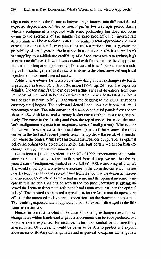
299 Exchange Rate Economics: What's Wrong with the Macro Approach?
alignments, whereas the former is between high interest rate differentials andexpected depreciation relative to central parity. For a sample period duringwhich a realignment is expected with some probability but does not occurowing to the shortness of the sample (the peso problem), high interest ratedifferentials will be associated with future realized total appreciation, even ifexpectations are rational. If expectations are not rational but exaggerate theprobability of a realignment, for instance, in a situation in which a central bankis struggling to establish the credibility of a fixed exchange rate regime, highinterest rate differentials will be associated with future total realized apprecia-tions also for longer sample periods. Thus, central banks' interest rate smooth-ing within exchange rate bands may contribute to the often observed empiricalrejection of uncovered interest parity.
Additional evidence for interest rate smoothing within exchange rate bandsis presented in figure 8C.1 (from Svensson [1994, fig. 2d]; see that paper fordetails). The top panel's thin curve shows a time series of deviations from cen-tral parity of the Swedish krona (relative to the currency basket that the kronawas pegged to prior to May 1992 when the pegging to the ECU [Europeancurrency unit] began). The horizontal dotted lines show the bandwidth, ±1.5percentage points. The thin curves in the second and third panels from the topshow the Swedish krona and currency basket one-month interest rates, respec-tively. The curve in the fourth panel from the top shows estimates of the mar-ket's realignment expectations (expected rates of realignment). Whereas thethin curves show the actual historical development of these series, the thickcurves in the first and second panels from the top show the result of a simula-tion where the central bank faces historical disturbances but pursues an optimalpolicy according to an objective function that puts certain weight on both ex-change rate and interest rate smoothing.
Let us look at just one incident. In the fall of 1990, expectations of a devalu-ation rose dramatically. In the fourth panel from the top, we see that the ex-pected rate of realignment peaked in the fall of 1990. Everything else equal,this would show up in a one-to-one increase in the domestic-currency interestrate. Instead, we see in the second panel from the top that the domestic interestrate increased by much less (the actual increase and the optimal increase coin-cide in this incident). As can be seen in the top panel, Sveriges Riksbank al-lowed the krona to depreciate within the band (somewhat less than the optimalpolicy). This created an expected appreciation for the krona that dampened theeffect of the increased realignment expectations on the domestic interest rate.The resulting expected rate of appreciation of the krona is displayed in the fifthpanel from the top.
Hence, in contrast to what is the case for floating exchange rates, for ex-change rates within bands exchange rate movements can be both predicted andto some extent explained, for instance, in terms of central banks smoothinginterest rates. Of course, it would be better to be able to predict and explainmovements of floating exchange rates and in general to explain exchange rate

300 Robert P. Flood and Mark P. Taylor
CMCM
(0
%
1?
tj
B
B7
87
88
88
09
69
90
90
91
91
93
Fig. 8C.1 Evidence of interest rate smoothingNote: x is percentage deviation of exchange rate from central parity; iT and z*T are domestic andforeign one-month interest rates, respectively; gT is expected rate of realignment; T equals fourweeks, dt = one week. Thin curve: actual. Thick curve: optimal. Dashed line: mean. For details,see Svensson (1994).
levels in terms of levels of other contemporaneous macro variables, but it isstill of some interest that exchange rate movements within bands are systematicand also not exclusively characterized by mean reversion.
I missed in Flood and Taylor's survey a discussion of international macroproblems or puzzles where a microstructure approach might help. A list ofsuch problems/puzzles is discussed extensively in Andrew Rose's comment onFlood and Taylor. Let me just mention two such problems/puzzles that areon my own wish list.
The effects on exchange rates of sterilized central bank intervention may besuitable to analyze with a microstructure approach. Most macro studies findlittle or no effect of sterilized intervention. If they are correct, why do central

301 Exchange Rate Economics: What's Wrong with the Macro Approach?
banks keep doing it? Some studies emphasize a signaling effect, namely, thatsterilized interventions signal future nonsterilized interventions. If the signal-ing effect is the important one, why are central banks often secretive abouttheir interventions? And why aren't there better ways to signal changes in futuremonetary policy?
Some central bank officials have suggested to me that herd behavior in theforeign exchange market may be exploited by central banks. If the central banksecretly through intermediaries can convey the impression that someone otherthan the central bank is suddenly starting to buy the currency, the herd mightfollow. This way the central bank would then be able to push or pull the ex-change rate in desired directions. These issues might be suitable for a micro-structure approach.
Another such issue is speculative attacks, in particular, central banks' de-fense against speculative attack. For instance, during the dramatic defense ofthe Swedish krona in September 1992, with a 500 percent overnight rate, theforeign exchange market for kronor and the Swedish Treasury bills marketseemed paralyzed. Instead of a strong inflow of kronor, very little trade oc-curred. Huge spreads were quoted on Swedish T-bills, indicating that no onewanted to trade. One reason is that it became almost impossible to price ashort-term bill since the uncertainty about the future overnight rate was enor-mous. Who knew whether it would come down to reasonable levels withinthree, seven, or fourteen days? A related issue is to what extent the increasedpractice of trading rules, dynamic hedging, etc. affects central banks' defenseagainst speculative attack. As the paper by Garber and Spencer (chap. 6 in thisvolume) demonstrates, this is another suitable area for a microstructureapproach.
References
Svensson, Lars E. O. 1993. Assessing target zone credibility: Mean reversion and deval-uation expectations in the ERM, 1979-1992. European Economic Review37:763-802.
. 1994. Why exchange rate bands: Monetary independence in spite of fixed ex-change rates. Journal of Monetary Economics 33:157-94.

Related Documents