Excess volatility? the Australian stock market from 1883 to 1999

Excess Volatility? The Australian Stock Marketfrom 1883 to 1999

by Richard Heaney, School of Finance and Applied Statistics, Faculty of Economics andCommerce, Australian National University, Canberra, Australia

Abstract

Are share markets too volatile? While it is difficult to ignore share market volatility it isimportant to determine whether volatility is excessive. This paper replicates the Shiller(1981) test as well as applying standard time series analysis to annual Australian stockmarket data for the period 1883 to 1999. While Shiller’s test suggests the possibility ofexcess volatility, time series analysis identifies a long-run relationship between sharemarket value and dividends, consistent with the share market reverting to its fundamentaldiscounted cash flow value over time.

JEL Classification: G12, C22, C32, C51, C52

Keywords: excess volatility, cointegration, unit root test, reversion to fundamental value

1. Introduction

There is considerable empirical evidence to support the argument that stock markets aremore volatile than the discounted cash flow pricing model suggests (Campbell and Shil-ler, 1987, Gillies and LeRoy, 1991, LeRoy, 1989, LeRoy and Porter, 1981, Scott, 1985,Shiller, 1981, 1988, 1990, and West, 1988a). While the work of Shiller (1981) and LeRoyand Porter (1981) publicised this argument, a fairly large number of empirical tests sup-porting the excess volatility argument followed. This additional work corrected many ofthe problems associated with the earlier research, including improved statistical tests aswell as alternative methods of analysis. Yet, during this period there was little success inexplaining the phenomenon (Gillies and LeRoy, 1991). It appears there is no acceptablereplacement for the discounted cash flow model. Bubbles and fads have been suggested(Gillies and LeRoy, 1991, Shiller, 1990 and West, 1988b) though West (1988b) arguesthat these explanations are not convincing. Two explanations that have generated sub-stantial interest are non-constant discount rates (Cochrane, 1992, Cuthbertson and Hyde,2002, Gillies and LeRoy, 1991, Kleidon, 1988b) and non-constant growth rates (Barskyand De Long, 1993) though these extensions are not the subject of this study.

Not all researchers accept that stock market prices are excessively volatile. For ex-ample, Ackert and Smith (1993), Barsky and De Long (1993), Cochrane (1992), Kleidon(1986a and 1986b), Marsh and Merton (1986) and Shea (1989) provide various rebuttals.While Shea (1989) questions some of the statistical tests applied in tests of excess volatil-ity, Ackert and Smith (1993) argue that care is required with the definition of dividendsparticularly in Shiller’s data set. Further, Barsky and De Long (1993), Kleidon (1986aand 1986b) and Marsh and Merton (1986) infer that Shiller’s result is peculiar to the as-sumed dividend process underlying the price calculation. They show that if dividends arenon-stationary then Shiller’s variance bounds are incorrect and the finding of excessvolatility is invalid.

Managerial Finance 76

This paper focuses on the question of excess stock market price volatility and theappropriateness of the discounted dividend valuation model using annual observations ofreal stock market value and real dividends for the Australian stock market. Unit root testsare applied in the analysis of the underlying processes driving real dividends and realstock market value, and tests for cointegration and vector error correction models areused in the analysis of the underlying relationship between these two variables. Theanalysis suggests that the value of the equity market tends to revert to its equilibrium orfundamental value over time even after substantial shocks such as the 1929 and 1987 eq-uity market crashes. The stock market data for the period from 1882 to 1999 was suppliedby the Australian Stock Exchange and an inflation index, the retail price index, was ob-tained from the Reserve Bank of Australia (section 3). The results from the analysis arereported in Section 4 and a summary is provided in Section 5. A review of the literature isprovided in the following section.

2. Literature Review

Shiller (1981) produced the most influential paper in this controversy. He argues thatstock returns are more volatile than suggested by the present value model. There are threekey assumptions underlying this analysis: constant growth rate, constant discount rate,and stationary dividend series. Shiller (1981) calculates real dividends and real stockmarket prices and detrends these series to remove an assumed constant geometric growthfactor. The traditional discounted cash flow model is relied upon to estimate the realstock market value, Pt, in terms of the present value of expected real dividends.

P E Dt

k

t t k

k

� ��

�

&

' 1

0

( ) (1)

where '��

1

1 r = constant real discount factor (0 < � < 1),

r = constant required return, r,

Et(.) = expectations operator as at time t,

Dt+k = real dividend k periods from time t paid at the end of the period t+k.

The long run growth is removed from Pt and Dt using a long run growth factor, 't-T

= (1+g)t-T, with g the growth rate and T the base year. Shiller(1981) estimates the growthrate by regressing the natural log of price on an intercept and time trend, ln(Pt) = a+bt+�t,and setting ' = eb. The real price and real dividends are adjusted for growth using thegrowth factor such that:

pP P

gd

D D

gt

t

t T

t

t T t

t

t T

t

t T� �

�� �

�� � � �� �( ) ( )1 1and (2)

Defining �'= '. The real stock market value as per equation (1) may now be rewrit-ten in terms of real growth adjusted expected dividends.

Volume 30 Number 1 2004 77

p E d E dt

k

t t k

k

t t k

kk

� ���

��

�

&

�

&

( )�' '1 1

00

(3)

The growth rate is defined to be less than the discount rate to ensure a finite price

and so it is expected that ' �'� ��

��

1

11

g

r. Shiller (1981) restates '�

�

1

1 rwhich is the

discount factor for the detrended real price, pt, and detrended real dividend series, dt. Thediscount rate is derived by taking unconditional expectations over equation (3) and sum-ming the resulting infinite series.

E p E E d E dk

t t k

k

k

k

( ) ( )��

!!

"

#$$� �

�

�

!

"

#$�

��

&�' '

'

'1

0

1

1�

&

0

E d( ) (4)

Given the definition of '��

1

1 r, the discount rate can be written as the ratio of the

mean growth adjusted real dividend to the mean growth adjusted real price or:

E pr

rE d

rE d( )

/ ( )

/ ( )( ) ( )�

�

� �

�

!

"

#$ �

1 1

1 1 1

1(5)

r E d E p� ( ) / ( ).

Thus the appropriate discount rate, r, for the adjusted series is estimated by takingthe ratio of expected value of the detrended real dividend to the expected value of the de-trended real price. Shiller (1981) suggests another formulation of the problem with theprice stated in terms of the actual (ex post) subsequent dividends:

p E p p dt t t t

k

t k

k

� � ��

�

&

( *) *where ' 1

0

(6)

Estimation of price using equation (6) involves summing over an infinite series ofdividend terms. The dividend process is estimated recursively by taking the averagegrowth adjusted real price from the full sample, E(p), as the present value of dividends atthe end of the sample. The price, pt*, is calculated beginning with the most recent obser-vation and then solving recursively back to the first observation using the equation:

p p dt t t* ( * )� ��'1

(7)

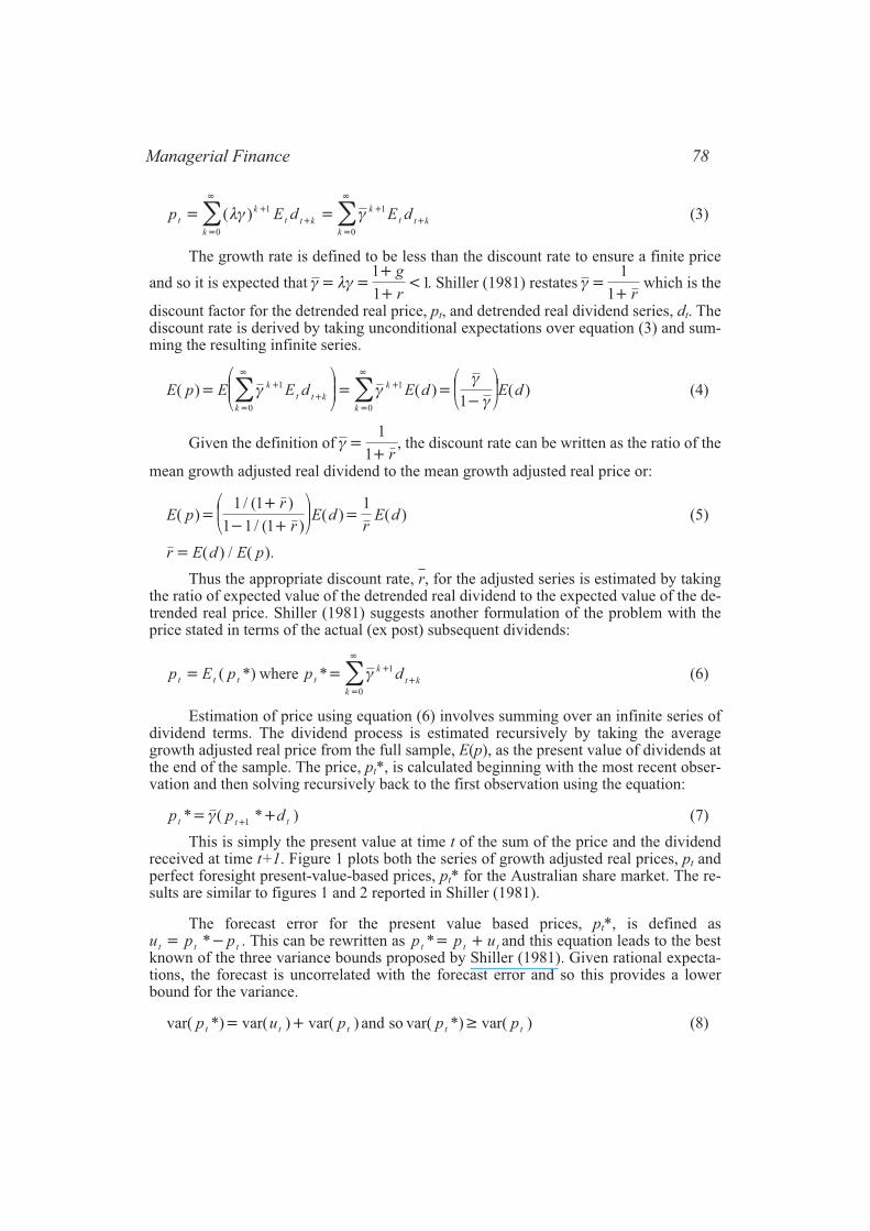
This is simply the present value at time t of the sum of the price and the dividendreceived at time t+1. Figure 1 plots both the series of growth adjusted real prices, pt andperfect foresight present-value-based prices, pt* for the Australian share market. The re-sults are similar to figures 1 and 2 reported in Shiller (1981).

The forecast error for the present value based prices, pt*, is defined asu p pt t t� �* . This can be rewritten as p p ut t t*� � and this equation leads to the bestknown of the three variance bounds proposed by Shiller (1981). Given rational expecta-tions, the forecast is uncorrelated with the forecast error and so this provides a lowerbound for the variance.

var( *) var( ) var( ) var( *) var( )p u p p pt t t t t� � �and so (8)

Managerial Finance 78

The bound1 is a hurdle value rather than a statistical test and the lack of a statisticaltest for significance generates some criticism. In the same year, LeRoy and Porter (1981)develop statistical tests of excess volatility supporting Shiller’s finding. Given these re-sults both Shiller (1981) and LeRoy and Porter (1981) reason that stock prices are toovolatile for the stock market to be efficient in a present value sense.

The suggestion that stock markets are excessively volatile has generated substantialdiscussion. For example Flavin (1983) and Kleidon (1986a) argue that Shiller’s variancebound tests are subject to a small sample bias towards rejection of the bounds. Marsh andMerton (1986) show the variance bounds tests are sensitive to the assumed dividend pro-cess and if dividends are non-stationary Shiller’s variance bounds are reversed. Kleidon(1986b) uses simulations to further highlight the impact of a non-stationary dividend pro-cess on Shiller’s variance bounds.2 While Gillies and LeRoy (1991) agree that an impor-tant criticism of the Shiller result is the reliance on the assumption of a stationarydividend process, they question whether this assumption can adequately explain the mag-nitude of the excess volatility observed by Shiller.

The assumption of a simple random walk process without drift provides an indica-tion of the impact of relaxing Shiller’s assumption of stationary dividends. In this case the

Volume 30 Number 1 2004 79

0

1000

2000

3000

4000

5000

6000

7000

18

83

18

90

18

97

19

04

19

11

19

18

19

25

19

32

19

39

19

46

19

53

19

60

19

67

19

74

19

81

19

88

19

95

Year

Sh

are

mark

et

valu

e

p*

p

Figure 1Share Price Index and Ex-Post Rational Price

(Real Prices and Dividends adjusted for Growth, 1883-1999)

Shar

eM

arket

Val

ue

Note:Both the real price and real dividend series are detrended by dividing by the long run exponentialgrowth factor and the base year is set at 1999. The variable p* is the present value of the observedsubsequent real detrended dividends with the present value of dividends at 1999 assumed equal tothe average real detrended price for the period. p* is calculated recursively beginning at 1999 withthe average real detrended price for the period and then the p* value for 1998 is calculated usingp p d1998 1998 1998* ( * )' � where dividends are received at the end of the period and ' is the discountrate.

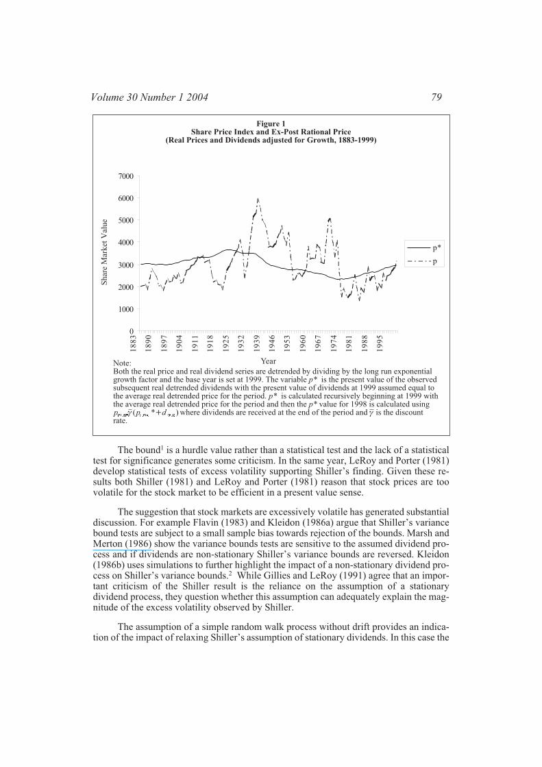
expected dividend for some time in the future is the current observed dividend or Etdt+k =dt (for all integers k > 0) and so given an infinite sequence of dividends, the stock marketvalue follows a simple perpetuity formula rather than requiring perfect knowledge of thefuture stream of dividends. Given equation (3):

p E dt

k

t t k

k

� ��

�

&

' 1

0

� � � �� �' ' 'E d E d E dt t t t t t

2

1

3

2�

� �� � � ��dt 1

21' ' ' �

��

���

dd

rt

t

1

1

1

'

'( )(9)

To provide some indication of the impact of this change in assumptions, the theo-retical price, pt*, is recalculated using the perpetuity formula detailed in equation (9) andthis is graphed in Figure 2. With this adjustment the volatility of the theoretical stockmarket value is much closer to the volatility of the actual market value.

Managerial Finance 80

0

1000

2000

3000

4000

5000

6000

7000

18

84

18

91

18

98

19

05

19

12

19

19

19

26

19

33

19

40

19

47

19

54

19

61

19

68

19

75

19

82

19

89

19

96

Year

share

mark

et

valu

e

p*

p

Shar

eM

arket

Val

ue

Figure 2Share Price Index and Valuation Based on Prior Dividend

(Real Prices and Dividends adjusted for Growth, 1883-1999)

Note:Both the real price and real dividend series are detrended by dividing by the long run exponentialgrowth factor and the base year is set at 1999. The variable p* is calculated using the constantdividend perpetuity model given the dividend for the previous period, observable now, and constantdiscount rate calculated for the sample, '. This is written as pt* = dt-1 / r.

One further criticism of the Shiller analysis involves the removal of the geometrictrend from the time series. While Nelson and Kang (1984) highlight the problems arisingfrom the removal of a deterministic trend from a non-stationary process, Kleidon(1986b), Marsh and Merton (1986) and Campbell and Shiller (1987) make this pointmore forcefully. Thus the removal of the impact of growth over the period may also ad-versely affect the conclusions drawn in early tests for excess volatility.

There are clearly problems with the early tests for excess volatility. As a result asecond generation of tests appeared in the literature (Gillies and LeRoy, 1991). Thesetests account for many of the problems identified in the earlier literature including adjust-ment for non-stationary dividends. Some of these tests (for example, Mankiw, Romer andShapiro, 1985 and 1991, Scott, 1985), though not all, identify excessive volatility. Onetest, developed by West (1988a) and applied in Ackert and Smith (1993), provides an im-portant example of the impact of limiting analysis to the payment of cash dividends.While West (1988a) found evidence supporting the existence of excess volatility usingShiller’s original data, Ackert and Smith (1993) argue that the dividend data used by Shil-ler (1981) and West (1988a) is narrowly defined and ignores cash flows from share repur-chases and takeover distributions, alternative sources of cash particularly evident after1970 when Shiller’s graphical analysis is particularly persuasive. With the use of a morebroadly defined measure of shareholder cash receipts, Ackert and Smith (1993) find littleevidence of excessive volatility.

A series of papers by Campbell and Shiller (1987, 1988a and 1988b) also adjust forsome of the problems observed in the early excess volatility literature and there is littleclear rejection of the discounted cash flow model. Cochrane (1992) also considers thisquestion suggesting that changing discount rates provide an important explanation for theobserved variation in stock prices. In general, the more recent tests either provide supportfor the discount cash flow model or fail to provide a clear rebuttal of the present valuemodel.

Barsky and De Long (1993) propose that a non-constant dividend growth rate ex-plains the unexpected variation in stock market returns. Their reasoning is couchedwithin the Gordon (1962) model. They argue that Shiller’s constant growth rate adjust-ment is invalid, assuming that the natural log of real dividends follows a complex non-stationary process. This assumption appears reasonable given a crude model of value,real dividends multiplied by 20, accounts for over three fifths of the variation in long runchanges in stock market value.3 This simple approximation provides a substantial im-provement over the model used in Shiller (1981). Although, Barsky and De Long (1993)find that stock value is more volatile than expected they argue this greater volatility is ex-plained by variation in the dividend growth rate. Their adjusted pricing model accountsfor much of the long run variation in observed prices. Given this alternative view on divi-dend processes, Barsky and De Long (1993) argue the present value model “… retainsconsiderable power.”

Thus there is still some uncertainty about the ability of the discounted cash flowmodel to explain observed stock market volatility. Possible explanations include model-ling time-varying dividend growth rates (Barsky and De Long, 1993) and time-varyingdiscount rates (Cochrane, 1992) though the task of assessing these alternative explana-tions is left to future research.

Volume 30 Number 1 2004 81

3. Data

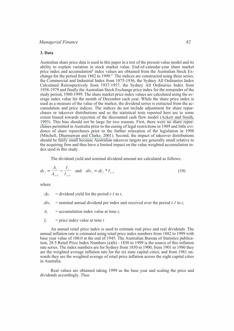
Australian share price data is used in this paper in a test of the present value model and itsability to explain variation in stock market value. End-of-calendar-year share marketprice index and accumulation4 index values are obtained from the Australian Stock Ex-change for the period from 1882 to 1999.5 The indices are constructed using three series,the Commercial and Industrial Index from 1875-1936, the Sydney All Ordinaries IndexCalculated Retrospectively from 1937-1957, the Sydney All Ordinaries Index from1958-1979 and finally the Australian Stock Exchange price index for the remainder of thestudy period, 1980-1999. The share market price index values are calculated using the av-erage index value for the month of December each year. While the share price index isused as a measure of the value of the market, the dividend series is extracted from the ac-cumulation and price indices. The indices do not include adjustment for share repur-chases or takeover distributions and so the statistical tests reported here are to someextent biased towards rejection of the discounted cash flow model (Ackert and Smith,1993). This bias should not be large for two reasons. First, there were no share repur-chases permitted in Australia prior to the easing of legal restrictions in 1989 and little evi-dence of share repurchases prior to the further relaxation of the legislation in 1998(Mitchell, Dharmawan and Clarke, 2001). Second, the impact of takeover distributionsshould be fairly small because Australian takeover targets are generally small relative tothe acquiring firm and thus have a limited impact on the value weighted accumulation in-dex used in this study.

The dividend yield and nominal dividend amount are calculated as follows:

dyA

A

I

Idiv dy It

t

t

t

t

t t t� � �

� ��

1 1

1and * (10)

where

dyt = dividend yield for the period t-1 to t,

divt = nominal annual dividend per index unit received over the period t-1 to t,

At = accumulation index value at time t,

It = price index value at time t

An annual retail price index is used to estimate real price and real dividends. Theannual inflation rate is estimated using retail price index numbers from 1882 to 1999 withbase year value of 100.0 at the end of 1945. The Australian Bureau of Statistics publica-tion, 28.5 Retail Price Index Numbers (a)(b) - 1850 to 1999 is the source of this inflationrate series. The index numbers are for Sydney from 1850 to 1900; from 1901 to 1980 theyare the weighted average inflation rate for the six state capital cities; and from 1981 on-wards they are the weighted average of retail price inflation across the eight capital citiesin Australia.

Real values are obtained taking 1999 as the base year and scaling the price anddividends accordingly. Thus

Managerial Finance 82

P I D divt t

b

t

t t

b

t

� �* **

*

*

*and (11)

where *t is the inflation index at time t. and *d is the inflation index at the base year,1999. The natural log of real dividends and the natural log the real price are then calcu-lated for later analysis.

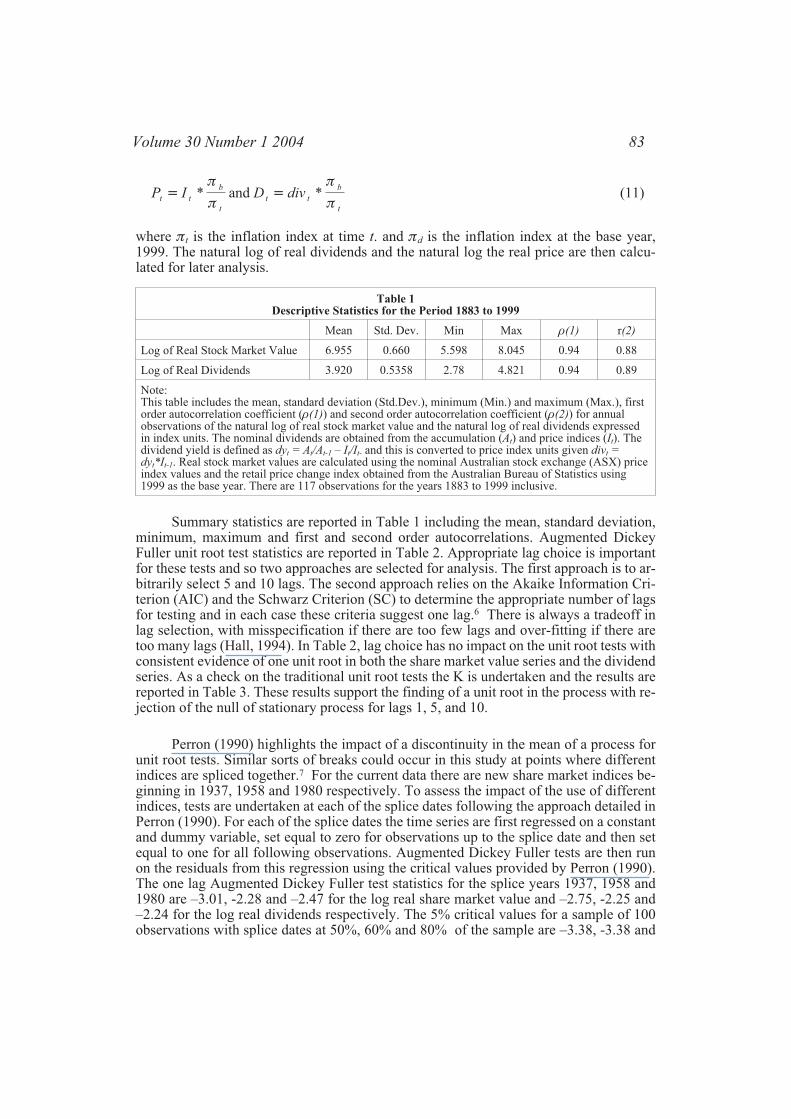
Table 1Descriptive Statistics for the Period 1883 to 1999

Mean Std. Dev. Min Max �(1) r(2)

Log of Real Stock Market Value 6.955 0.660 5.598 8.045 0.94 0.88

Log of Real Dividends 3.920 0.5358 2.78 4.821 0.94 0.89

Note:This table includes the mean, standard deviation (Std.Dev.), minimum (Min.) and maximum (Max.), firstorder autocorrelation coefficient (�(1)) and second order autocorrelation coefficient (�(2)) for annualobservations of the natural log of real stock market value and the natural log of real dividends expressedin index units. The nominal dividends are obtained from the accumulation (At) and price indices (It). Thedividend yield is defined as dyt = At/At-1 – It/It- and this is converted to price index units given divt =dyt*It-1. Real stock market values are calculated using the nominal Australian stock exchange (ASX) priceindex values and the retail price change index obtained from the Australian Bureau of Statistics using1999 as the base year. There are 117 observations for the years 1883 to 1999 inclusive.

Summary statistics are reported in Table 1 including the mean, standard deviation,minimum, maximum and first and second order autocorrelations. Augmented DickeyFuller unit root test statistics are reported in Table 2. Appropriate lag choice is importantfor these tests and so two approaches are selected for analysis. The first approach is to ar-bitrarily select 5 and 10 lags. The second approach relies on the Akaike Information Cri-terion (AIC) and the Schwarz Criterion (SC) to determine the appropriate number of lagsfor testing and in each case these criteria suggest one lag.6 There is always a tradeoff inlag selection, with misspecification if there are too few lags and over-fitting if there aretoo many lags (Hall, 1994). In Table 2, lag choice has no impact on the unit root tests withconsistent evidence of one unit root in both the share market value series and the dividendseries. As a check on the traditional unit root tests the K is undertaken and the results arereported in Table 3. These results support the finding of a unit root in the process with re-jection of the null of stationary process for lags 1, 5, and 10.

Perron (1990) highlights the impact of a discontinuity in the mean of a process forunit root tests. Similar sorts of breaks could occur in this study at points where differentindices are spliced together.7 For the current data there are new share market indices be-ginning in 1937, 1958 and 1980 respectively. To assess the impact of the use of differentindices, tests are undertaken at each of the splice dates following the approach detailed inPerron (1990). For each of the splice dates the time series are first regressed on a constantand dummy variable, set equal to zero for observations up to the splice date and then setequal to one for all following observations. Augmented Dickey Fuller tests are then runon the residuals from this regression using the critical values provided by Perron (1990).The one lag Augmented Dickey Fuller test statistics for the splice years 1937, 1958 and1980 are –3.01, -2.28 and –2.47 for the log real share market value and –2.75, -2.25 and–2.24 for the log real dividends respectively. The 5% critical values for a sample of 100observations with splice dates at 50%, 60% and 80% of the sample are –3.38, -3.38 and

Volume 30 Number 1 2004 83

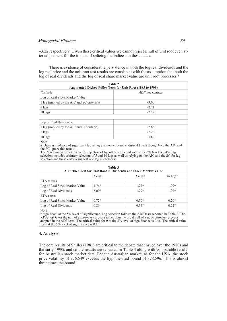
–3.22 respectively. Given these critical values we cannot reject a null of unit root even af-ter adjustment for the impact of splicing the indices on these dates.

There is evidence of considerable persistence in both the log real dividends and thelog real price and the unit root test results are consistent with the assumption that both thelog of real dividends and the log of real share market value are unit root processes.8

Table 2Augmented Dickey Fuller Tests for Unit Root (1883 to 1999)

Variable ADF test statistic

Log of Real Stock Market Value

1 lag (implied by the AIC and SC criteria)# -3.00

5 lags -2.71

10 lags -2.52

Log of Real Dividends

1 lag (implied by the AIC and SC criteria) -2.86

5 lags -2.26

10 lags -1.62

Note# There is evidence of significant lag at lag 8 at conventional statistical levels though both the AIC andthe SC ignore this result.The MacKinnon critical value for rejection of hypothesis of a unit root at the 5% level is 3.45. Lagselection includes arbitrary selection of 5 and 10 lags as well as relying on the AIC and the SC for lagselection and these criteria suggest one lag in each case.

Table 3A Further Test for Unit Root in Dividends and Stock Market Value

1 Lag 5 Lags 10 Lags

ETA � tests

Log of Real Stock Market Value 4.76* 1.73* 1.02*

Log of Real Dividends 5.00* 1.79* 1.04*

ETA + tests

Log of Real Stock Market Value 0.72* 0.30* 0.20*

Log of Real Dividends 0.86 0.34* 0.22*

Note* significant at the 5% level of significance. Lag selection follows the ADF tests reported in Table 2. TheKPSS test takes the null of a stationary process rather than the usual null of a non-stationary processadopted in the ADF tests. The critical value for � at the 5% level of significance is 0.46. The critical valuefor � at the 5% level of significance is 0.15.

4. Analysis

The core results of Shiller (1981) are critical to the debate that ensued over the 1980s andthe early 1990s and so the results are repeated in Table 4 along with comparable resultsfor Australian stock market data. For the Australian market, as for the USA, the stockprice volatility of 976.549 exceeds the hypothesised bound of 378.596. This is almostthree times the bound.

Managerial Finance 84

Table 4Comparison of the Shiller (1981) Based Estimates for the USA and Australia

Australian StockExchange Share Price Data

Shiller (1981), S&PIndexData

Shiller (1981), ModifiedDow IndustrialData

Sample period 1883-1999 1871-1979 1928-1979

E(p) 2967.463 145.500 982.600

E(d) 140.201 6.989 44.760

r = E(d)/E(p) 0.047 0.048 0.456

r2 = (1+r)2-1 0.097 0.098 0.093

b = ln(�) 0.017 0.015 0.019

�(b) (0.001) (0.001) (1.004)

cor(p,p*) 0.193 0.392 0.163

�(d) 36.575 1.481 9.828

Volatility estimates

�(p) 976.549 50.120 355.900

�(p*) 378.596 8.968 25.800

Note:The choice of parameters estimated for Australian Stocks and for US stocks follow Shiller (1981). Prices,p, and dividends, d, are inflation adjusted and adjusted for growth, �, over the period with expected valuesof E(p) and E(d). For the Australian data the base year is set at 1999. The price, p*, is calculatedbeginning in 1999, assuming the average growth adjusted real price for the sample, E(p) reflects the priceat the end of 1999 and then discounting the sum of dividends and the ex post rational price at the end ofthe period using the discount rate as r per equation (7).

Kleidon (1986b) showed if the dividends follow a random walk then the best esti-mate of future dividends is the dividend just observed. To gauge the impact of this changein assumption, the bound is re-estimated by assuming the real price is adequately repre-

sented by the perpetuity,d

r

t�1where current dividends are the best estimate of future divi-

dends. This results in doubling of the bound from 378.596 to 812.882. The argument forexcess volatility is now far less convincing. In Figure 2 the theoretical price is muchcloser to the observed stock market value and the new theoretical price exhibits volatilitylevels much closer to those observed in the share market. The arguments of Barsky andDe Long (1993), Kleidon (1986a, 1986b, 1988a and 1988b) and Marsh and Merton(1986) concerning the assumed underlying dividend process seem well founded.

Shiller also assumed the data could be detrended in a meaningful way. If both realdividend and real price follow unit root processes then detrending is not valid (Nelsonand Kang, 1984). Given the results of unit root tests reported in the previous section thedetrending technique applied in the original Shiller (1981) paper is flawed (Kleidon,1986a, 1986b, 1988a and 1988b and Marsh and Merton, 1986).

Barsky and De Long (1993) and Campbell and Shiller (1988b) suggest the possibil-ity of a long run relationship between real price and real dividends. Following the litera-ture, the real price is defined in terms of the Gordon (1962) model with constant dividendgrowth.

Volume 30 Number 1 2004 85

PD g

r gt

t��

�

( )

( )

1(12)

Taking logs and rearranging equation (12) we obtain:

ln( ) ln ln( ) ln( )Pg

r gD c Dt t t�

�

�

�

!

"

#$� � �

1(13)

Given a constant discount factor (c), there is a linear relationship between the logreal price, the discount factor and the log real dividends. Johansen tests for cointegrationare conducted to test for evidence of this linear relationship between log real dividendsand log real price for the Australian market. The results, reported in Table 5, identify onecointegrating vector and this result is insensitive both to the choice of statistic and to thelag choice (one through 10). The cointegrating vector, using a two-lag model, is (1,-2.165, -1.222). This means that, given equation (13), the share market value parameter isone, the discount factor parameter is -2.165 and the dividend parameter is –1.222.

Table 5Johansen Tests for Cointegration

Eigenvalue Statistic 5 percent criticalvalue

Trace statistic

No cointegrating vectors 0.140 19.220* 15.41

At most one cointegrating vector 0.017 2.010 3.76

Maximum eigen-value statistic

No cointegrating vectors 0.140 17.211* 14.07

At most one cointegrating vector 0.017 2.010 3.76

Note: * denotes rejection of the hypothesis at the 5% level. The test statistics reported here are for aVECM of order two with intercept in both the VAR and the error correction vector. Lag selection is basedon a general to specific search starting from 10 lags. The trace test indicates 1 cointegrating vector at the5% level. The Maximum eigen-value test also indicates there is one cointegrating vector at the 5% level.The test was also conducted for lags 1 through 10 with no change in the finding of one cointegratingvector at the 5% level of significance.

If two time series are cointegrated then the time series have a vector error correc-tion model representation (Banerjee, Dolado, Galgraith and Hendry, 1993) and so a vec-tor error correction model is used in the following analysis. This facilitates analysis of theimpact of the longer-run effects (error correction term) as well as identifying the impactof short-run lead/lag relationships between dividends and stock market value. An impor-tant task in estimation of the vector error correction model is identification of an appro-priate number of lag terms. A commonly used approach is the initial identification of ageneral model (10 lags in this case), which is reduced to a specific, more parsimonious,model using F-tests and t-tests to remove statistically insignificant lags. The final modelobtained using this approach includes two lags. The AIC and SC criteria were also usedthough both suggested inclusion of only one lag. While the one-lag model exhibited sub-stantial serial correlation in the residuals there was no evidence of statistically significant

Managerial Finance 86

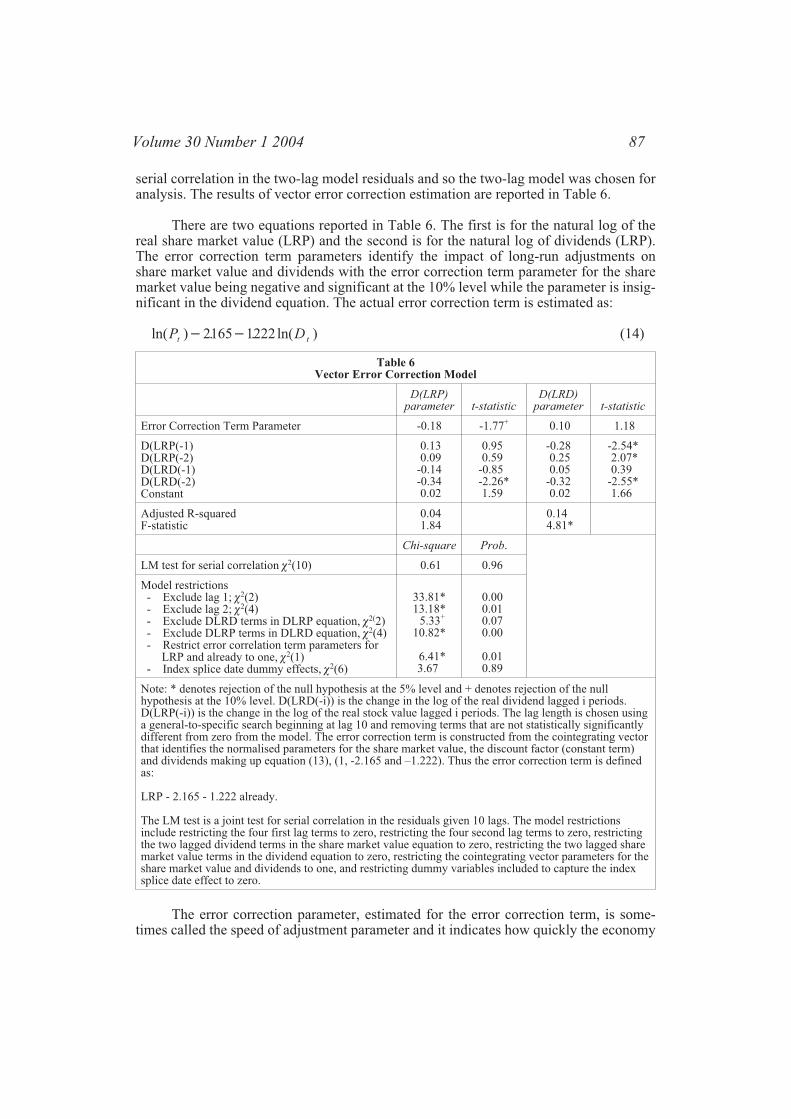
serial correlation in the two-lag model residuals and so the two-lag model was chosen foranalysis. The results of vector error correction estimation are reported in Table 6.

There are two equations reported in Table 6. The first is for the natural log of thereal share market value (LRP) and the second is for the natural log of dividends (LRP).The error correction term parameters identify the impact of long-run adjustments onshare market value and dividends with the error correction term parameter for the sharemarket value being negative and significant at the 10% level while the parameter is insig-nificant in the dividend equation. The actual error correction term is estimated as:

ln( ) . . ln( )P Dt t� �2165 1222 (14)

Table 6Vector Error Correction Model

D(LRP)parameter t-statistic

D(LRD)parameter t-statistic

Error Correction Term Parameter -0.18 -1.77+ 0.10 1.18

D(LRP(-1)D(LRP(-2)D(LRD(-1)D(LRD(-2)Constant

0.130.09

-0.14-0.340.02

0.950.59

-0.85-2.26*1.59

-0.280.250.05

-0.320.02

-2.54*2.07*0.39

-2.55*1.66

Adjusted R-squaredF-statistic

0.041.84

0.144.81*

Chi-square Prob.

LM test for serial correlation (2(10) 0.61 0.96

Model restrictions- Exclude lag 1; (2(2)- Exclude lag 2; (2(4)- Exclude DLRD terms in DLRP equation, (2(2)- Exclude DLRP terms in DLRD equation, (2(4)- Restrict error correlation term parameters for

LRP and already to one, (2(1)- Index splice date dummy effects, (2(6)

33.81*13.18*

5.33+

10.82*

6.41*3.67

0.000.010.070.00

0.010.89

Note: * denotes rejection of the null hypothesis at the 5% level and + denotes rejection of the nullhypothesis at the 10% level. D(LRD(-i)) is the change in the log of the real dividend lagged i periods.D(LRP(-i)) is the change in the log of the real stock value lagged i periods. The lag length is chosen usinga general-to-specific search beginning at lag 10 and removing terms that are not statistically significantlydifferent from zero from the model. The error correction term is constructed from the cointegrating vectorthat identifies the normalised parameters for the share market value, the discount factor (constant term)and dividends making up equation (13), (1, -2.165 and –1.222). Thus the error correction term is definedas:

LRP - 2.165 - 1.222 already.

The LM test is a joint test for serial correlation in the residuals given 10 lags. The model restrictionsinclude restricting the four first lag terms to zero, restricting the four second lag terms to zero, restrictingthe two lagged dividend terms in the share market value equation to zero, restricting the two lagged sharemarket value terms in the dividend equation to zero, restricting the cointegrating vector parameters for theshare market value and dividends to one, and restricting dummy variables included to capture the indexsplice date effect to zero.

The error correction parameter, estimated for the error correction term, is some-times called the speed of adjustment parameter and it indicates how quickly the economy

Volume 30 Number 1 2004 87

moves back to the long run equilibrium level after a shock. Assume the economy is inequilibrium with an error correction term equal to zero. If there is a positive shock to divi-dends then equation (14) shows that the error correction term will become negative. Toassess the impact of this shock on future share market value it should be noted that theproduct of the error correction term and error correction parameter (-0.18 in Table 6) ispositive. Thus the long-run effect of a positive shock to dividends is initially an increasein the next period share market value and, in the absence of further shocks, the error cor-rection term will ultimately drive the share market value up to its new equilibrium levelconsistent with the increase in dividends. Dividends appear to be exogenous with respectto long-run pricing errors because there is no statistically significant error correction pa-rameter in the dividend equation.

The dividend parameter in the cointegrating vector is equal to 1.222 and this pa-rameter is statistically significantly greater than one as indicated by the chi-square teststatistic of 6.41 in Table 6, a result that is also observed in the long-return regression re-ported in Barsky and De Long (1993).

The intercept term, or discount factor, in the cointegrating vector also providessome information about the Australian share market. If the growth rate is set at the aver-age over the period, 1.7% (Table 4), then the intercept estimate of 2.165 suggests a stockmarket discount rate of around 13.4%. This seems a little high given the continuouslycompounded real stock market return mean of 6.8% and median of 8.4% for the period1883 to 1999. Further, this is also high when compared with the geometric average of8.26% reported in Officer (1989) as an estimate for the Australian share market risk pre-mium for the period 1882 to 1987. Although the full estimation details are not reportedhere, it is found that when the vector error correction model is re-estimated with the divi-dend parameter constrained to one the constrained error correction term takes the form:

ln( ) . ln( )P Dt t� �3036 (15)

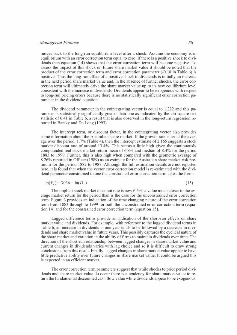
The implicit stock market discount rate is now 6.5%, a value much closer to the av-erage market return for the period than is the case for the unconstrained error correctionterm. Figure 3 provides an indication of the time changing nature of the error correctionterm from 1883 through to 1999 for both the unconstrained error correction term (equa-tion 14) and for the constrained error correction term (equation 15).

Lagged difference terms provide an indication of the short-run effects on sharemarket value and dividends. For example, with reference to the lagged dividend terms inTable 6, an increase in dividends in one year tends to be followed by a decrease in divi-dends and share market value in future years. This possibly captures the cyclical nature ofthe share market and variation in the ability of firms to maintain dividends over time. Thedirection of the short-run relationship between lagged changes in share market value andcurrent changes in dividends varies with lag choice and so it is difficult to draw strongconclusions from this result. Finally, lagged changes in share market value appear to havelittle predictive ability over future changes in share market value. It could be argued thisis expected in an efficient market.

The error correction term parameters suggest that while shocks to prior period divi-dends and share market value do occur there is a tendency for share market value to re-turn the fundamental discounted cash flow value while dividends appear to be exogenous.

Managerial Finance 88

Further, the results suggest that there are feedback effects from dividends to share marketvalue and from share market value to dividends in the short-run.

5. Conclusions

The arguments of Shiller (1981) appear to be a little too pessimistic for the Australianstock market though the results of this paper also indicate the need for some care in theuse of the discounted cash flow model. Holding the discount rate and the growth rate con-stant over the study period, there is evidence of a long-run relationship with share marketvalue reacting to previous period dividend shocks or to share market value shocks. Theselong-run effects tend to drive share market value back to its fundamental value. Thelong-run fundamental value is roughly consistent with the discounted cash flow modelwith log prices a linear function of log dividends though the one-to-one movement pre-dicted by the discounted cash flow model is not observed. It appears stock market price ismore sensitive to dividend variation than predicted. Though the parameter estimate of1.222 is fairly close, it is statistically significantly different from the predicted value of1.000. Nevertheless, the discounted cash flow model explains much of the long run varia-tion in stock market value. There is also some evidence of short-term effects though theseeffects are not the topic of this paper.

Volume 30 Number 1 2004 89

-0.6

-0.4

-0.2

0

0.2

0.4

0.6

18

83

18

89

18

95

19

01

19

07

19

13

19

19

19

25

19

31

19

37

19

43

19

49

19

55

19

61

19

67

19

73

19

79

19

85

19

91

19

97

unconstrained ECT

constrained ECT

Figure 3Long Run Pricing Errors

Note: The long run pricing errors, or error correction terms (ECT), are defined as per equation(14) and equation (15). Equation (14) describes the unconstrained ECT equation and equation(15), where the share market value and dividend parameters are constrained to equal to one,describes the constrained ECT equation. These equations reflect the long run changes in therelationship between real price and real dividends over time.

Stock market value appears to be anchored to the long run relationship identified inthe cointegrating vector though there are periods where considerable discrepancies exist.Perhaps these periods of pricing discrepancy could be explained by variation in dividendgrowth (Barsky and De Long, 1993) and time varying discount rate (Cochrane, 1992).This certainly provides a question for future research.

Acknowledgements

I would like to express my appreciation to Dr Grant Fleming at the ANU for his encour-agement in the early stages of this project and to the editor, Ron Balvers, whose generoushelp and guidance is much appreciated and to an anonymous referee for their commentsand suggestions

* Correspondence to Richard Heaney, School of Finance and Applied Statistics, Austra-lian National University, Canberra ACT 0200, Australia. Phone: 61 2 61254726, E-mail:[email protected]

Managerial Finance 90

Endnotes

1. Shiller develops two other variance bounds though these add little to the discussion asthe results are consistent for each of the bounds.

2. In a later paper, Shiller (1988) criticises Kleidon’s simulations because they appear tobe sensitive to parameter choice.

3. This is strikingly close to discounting real dividends in perpetuity at the real share mar-ket discount rate of around 5% observed in a number of the studies.

4. The accumulation index includes the impact of dividends as well as changes in value.

5. The Australian Stock Exchange has only recently made this data available. A similarindex was used in estimation of equity premia by Officer (1989) and in analysis of timechanging volatility in Kearns and Pagan (1993).

6. An anonymous reviewer suggested this alternative approach.

7. The need for testing for this effect was raised by an anonymous reviewer. Each splicingpoint is tested individually in this paper though an alternative approach, not followedhere, is to test all three of the splice points jointly.

8. Note that the unit root process for log real price indicates there is no simple meanreversion of real share market value toward its long run average. The following analysissuggests that the share market reverts to its long run fundamental value determined by thediscounted cash flow model.

Volume 30 Number 1 2004 91

References

Ackert, Lucy, F. and Smith, Brian F., 1993, “Stock Price Volatility, Ordinary Dividends,and Other Cash Flows to Shareholders”, Journal of Finance, 48, 4, 1147-1160.

Banerjee, Anindya, Dolado, Juan, J., Galgraith, John, W. and Hendry, David, F., 1993,Co-Integration, Error-Correction, and the Econometric Analysis of Non-StationaryData, Oxford University Press, Oxford.

Barsky, Robert, B. and J. Bradford De Long, 1993, “Why Does the Stock Market Fluctu-ate”, Quarterly Journal of Economics, 108, 2, 291-311.

Campbell, John. Y. and Shiller, Robert. J., 1987, “Cointegration and Tests of PresentValue Models”, Journal of Political Economy, 95, 1062-1088.

Campbell, John. Y. and Shiller, Robert. J., 1988a, “Stock Prices, Earnings, and ExpectedDividends”, Journal of Finance, 43, 661-676.

Campbell, John. Y. and Shiller, Robert. J., 1988b, “The Dividend-Price Ratio and Expec-tations of Future Dividends and Discount Factors”, Review of Financial Studies, 3, 195-228.

Cochrane, John, H., 1992, “Explaining the Variance of Price-Dividend Ratios”, Reviewof Financial Studies, 5, 243-280.

Cuthbertson, Keith and Stuart Hyde, 2002, “Excess Volatility and Efficiency in Frenchand German Markets”, Economic Modelling, 19, 399-418.

Flavin, Marjorie A., 1983, “Excess Volatility in the Financial Markets: A reassessment ofthe Empirical Evidence”, Journal of Political Economy, 91, 6, 929-956.

Gillies, Christian and LeRoy, Stephen, F., 1991, “Econometric Aspects of the Variance-Bounds tests: A Survey”, Review of Financial Studies, 4, 4, 753-791.

Gordon, Myron, 1962, The Investment, Financing and Valuation of the Corporation, Ir-win, Homewood, IL.

Hall, Alistair, 1994, “Testing for a Unit Root in Time Series with Pretest Data-BasedModel Selection”, Journal of Business and Economic Statistics, 12, 4, 481-470.

Kleidon, Allan, W., 1986a, “Bias in Small Sample Tests of stock Price Rationality”,Journal of Business, 59, 2, 237-261.

Kleidon, Allan, W., 1986b, “Variance Bounds Tests and Stock Price Valuation Models”,The Journal of Political Economy, 94, 5, 953-1001.

Managerial Finance 92

Kleidon, Allan, W., 1988a, “The Probability of Gross Violations of a Present Value Vari-ance Inequality: Reply”, The Journal of Political Economy, 96, 5, 1093-1096.

Kleidon, Allan, W., 1988b, “Bubbles, Fads and Stock Price Volatility Tests: A PartialEvaluation: Discussion”, The Journal of Finance, 43, 3, 656-660.

LeRoy, Stephen, F., 1989, “Efficient Capital Markets and Martingales”, Journal of Eco-nomic Literature, 27, 4, 1583-1621.

LeRoy, Stephen, F., and Porter, Richard D., 1981, “The Present Value Relation: TestsBased on Implied Variance Bounds”, Econometrica, 49, 3, 555-574.

Mankiw, N. G., D. Romer and M. D. Shapiro, 1985, “An Unbiased Reexamination ofStock Market Volatility”, Journal of Finance, 40, 677-687.

Mankiw, N. G., D. Romer and M. D. Shapiro, 1991, “Stock Market Forecastability andVolatility: A Statistical Appraisal”, Review of Economic Studies, 58, 455-477.

Marsh, Terry, A. and Robert C. Merton, 1986, “Dividend Variability and VarianceBounds Tests for the Rationality of Stock Market Prices”, American Economic Review,76, 3, 483-498.

Mitchell, Jason, D., Dharmawan, Grace V. and Clarke, Alex W., 2001, “Managements’Views on Share Buy-Backs: An Australian Survey”, Accounting and Finance, 41, 1/2,93-129.

Nelson, Charles, R. and Kang, Heejong, 1984, “Pitfalls in the Use of Time as an Explana-tory Variable in regression”, Journal of Business and Economic Statistics, 2, 1, 73-82.

Officer, R. R., 1989, “Rates of Return to Shares, Bond Yields and Inflation Rates: AnHistorical Perspective”, Share Markets and Portfolio Theory. R. Ball, P. Brown, F. J.Finn and R. R. Officer. St. Lucia, Qld., University of Queensland Press, 207-211

Pagan, Adrian, A. and Kearns, Phillip, 1993, “Australian Stock Market Volatility: 1875-1987”, Economic Record, 69, 205, 163-178.

Perron, Pierre, 1990, “Testing for a Unit Root in a Time Series with Changing Mean”,Journal of Business and Economic Statistics, 8, 2, 153-162.

Scott, Louis, O., 1985, “The Present Value Model of Stock Prices: Regression Tests andMonte Carlo Results”, The Review of Economics and Statistics, 67, 4, 599-605.

Shea, Gary, S., 1989, “Ex-Post Rational Price Approximations and the Empirical Reli-ability of the Present-Value Relation”, Journal of Applied Econometrics, 4, 2, 139-159.

Volume 30 Number 1 2004 93

Shiller, Robert, J., 1981, “Do Stock Prices Move Too Much to be Justified by SubsequentChanges in Dividends?”, The American Economic Review, 71, 3, 421-436.

Shiller, Robert, J., 1988, “The Probability of Gross Violations of a Present Value Vari-ance Inequality”, The Journal of Political Economy, 96, 5, 1089-1092.

Shiller, Robert, J., 1990, “Market Volatility and Investor Behavior”, The American Eco-nomic Review, 80, 2, 58-62.

West, Kenneth, D., 1988a, “Dividend Innovations and Stock Price Volatility”, Economet-rica, 56, 1, 37-61.

West, Kenneth, D., 1988b, “Bubbles, Fads and Stock Price Volatility Tests: A PartialEvaluation”, The Journal of Finance, 43, 3, 639-655.

Managerial Finance 94