© ACTEX 2008 SOA Exam C/CAS Exam 4 - Construction and Evaluation of Actuarial Models EXCERPTS FROM ACTEX STUDY MANUAL FOR SOA EXAM C/SOA EXAM 4 2008 Table of Contents for Volumes 1 and 2 Introductory Comments SECTION 4 - KERNEL SMOOTHING ESTIMATORS ME-31 PROBLEM SET 4 ME-45

Welcome message from author
This document is posted to help you gain knowledge. Please leave a comment to let me know what you think about it! Share it to your friends and learn new things together.
Transcript

© ACTEX 2008 SOA Exam C/CAS Exam 4 - Construction and Evaluation of Actuarial Models
EXCERPTS FROM ACTEX STUDY MANUALFOR SOA EXAM C/SOA EXAM 42008
Table of Contents for Volumes 1 and 2
Introductory Comments
SECTION 4 - KERNEL SMOOTHING ESTIMATORS ME-31PROBLEM SET 4 ME-45
© ACTEX 2008 SOA Exam C/CAS Exam 4 - Construction and Evaluation of Actuarial Models
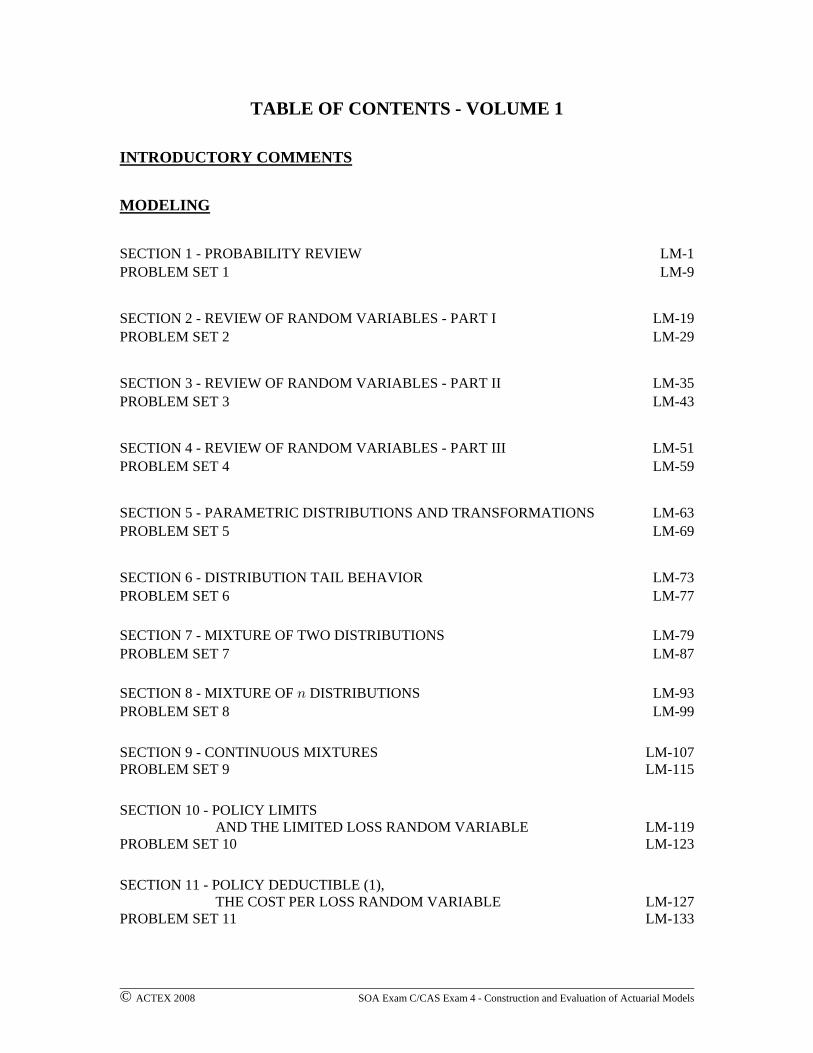
TABLE OF CONTENTS - VOLUME 1
INTRODUCTORY COMMENTS
MODELING
SECTION 1 - PROBABILITY REVIEW LM-1PROBLEM SET 1 LM-9
SECTION 2 - REVIEW OF RANDOM VARIABLES - PART I LM-19PROBLEM SET 2 LM-29
SECTION 3 - REVIEW OF RANDOM VARIABLES - PART II LM-35PROBLEM SET 3 LM-43
SECTION 4 - REVIEW OF RANDOM VARIABLES - PART III LM-51PROBLEM SET 4 LM-59
SECTION 5 - PARAMETRIC DISTRIBUTIONS AND TRANSFORMATIONS LM-63PROBLEM SET 5 LM-69
SECTION 6 - DISTRIBUTION TAIL BEHAVIOR LM-73PROBLEM SET 6 LM-77
SECTION 7 - MIXTURE OF TWO DISTRIBUTIONS LM-79PROBLEM SET 7 LM-87
SECTION 8 - MIXTURE OF DISTRIBUTIONS LM-938
PROBLEM SET 8 LM-99
SECTION 9 - CONTINUOUS MIXTURES LM-107PROBLEM SET 9 LM-115
SECTION 10 - POLICY LIMITS AND THE LIMITED LOSS RANDOM VARIABLE LM-119PROBLEM SET 10 LM-123
SECTION 11 - POLICY DEDUCTIBLE (1), THE COST PER LOSS RANDOM VARIABLE LM-127PROBLEM SET 11 LM-133

© ACTEX 2008 SOA Exam C/CAS Exam 4 - Construction and Evaluation of Actuarial Models
MODELING
SECTION 12 - POLICY DEDUCTIBLE (2), THE COST PER PAYMENT RANDOM VARIABLE LM-143PROBLEM SET 12 LM-149
SECTION 13 - POLICY DEDUCTIBLES APPLIED TO THE UNIFORM, EXPONENTIAL AND PARETO DISTRIBUTIONS LM-159PROBLEM SET 13 LM-167
SECTION 14 - COMBINED LIMIT AND DEDUCTIBLE LM-171PROBLEM SET 14 LM-177
SECTION 15 - ADDITIONAL POLICY ADJUSTMENTS LM-187PROBLEM SET 15 LM-191
SECTION 16 - MODELS FOR THE NUMBER OF CLAIMS AND THE CLASS LM-195Ð+ß ,ß !ÑPROBLEM SET 16 LM-203
SECTION 17 - MODELS FOR THE AGGREGATE LOSS, COMPOUND DISTRIBUTIONS (1) LM-213PROBLEM SET 17 LM-217
SECTION 18 - COMPOUND DISTRIBUTIONS (2) LM-239PROBLEM SET 18 LM-245
SECTION 19 - MORE PROPERTIES OF THE AGGREGATE LOSS RANDOM VARIABLE LM-257PROBLEM SET 19 LM-261
SECTION 20 - STOP LOSS INSURANCE LM-275PROBLEM SET 20 LM-281
SECTION 21 - DISCRETE TIME RUIN MODELS LM-285PROBLEM SET 21 LM-289
© ACTEX 2008 SOA Exam C/CAS Exam 4 - Construction and Evaluation of Actuarial Models
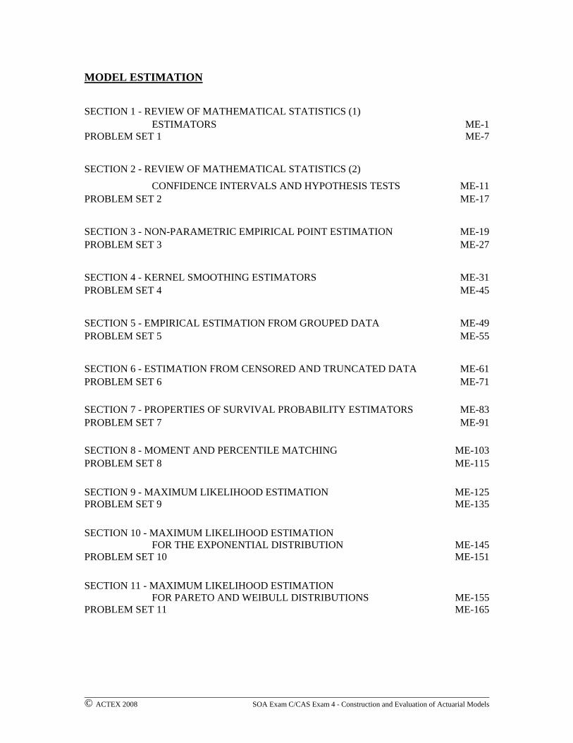
MODEL ESTIMATION
SECTION 1 - REVIEW OF MATHEMATICAL STATISTICS (1) ESTIMATORS ME-1PROBLEM SET 1 ME-7
SECTION 2 - REVIEW OF MATHEMATICAL STATISTICS (2) CONFIDENCE INTERVALS AND HYPOTHESIS TESTS ME-11PROBLEM SET 2 ME-17
SECTION 3 - NON-PARAMETRIC EMPIRICAL POINT ESTIMATION ME-19PROBLEM SET 3 ME-27
SECTION 4 - KERNEL SMOOTHING ESTIMATORS ME-31PROBLEM SET 4 ME-45
SECTION 5 - EMPIRICAL ESTIMATION FROM GROUPED DATA ME-49PROBLEM SET 5 ME-55
SECTION 6 - ESTIMATION FROM CENSORED AND TRUNCATED DATA ME-61PROBLEM SET 6 ME-71
SECTION 7 - PROPERTIES OF SURVIVAL PROBABILITY ESTIMATORS ME-83PROBLEM SET 7 ME-91
SECTION 8 - MOMENT AND PERCENTILE MATCHING ME-103PROBLEM SET 8 ME-115
SECTION 9 - MAXIMUM LIKELIHOOD ESTIMATION ME-125PROBLEM SET 9 ME-135
SECTION 10 - MAXIMUM LIKELIHOOD ESTIMATION FOR THE EXPONENTIAL DISTRIBUTION ME-145PROBLEM SET 10 ME-151
SECTION 11 - MAXIMUM LIKELIHOOD ESTIMATION FOR PARETO AND WEIBULL DISTRIBUTIONS ME-155PROBLEM SET 11 ME-165

© ACTEX 2008 SOA Exam C/CAS Exam 4 - Construction and Evaluation of Actuarial Models
MODEL ESTIMATION
SECTION 12 - MAXIMUM LIKELIHOOD ESTIMATION FOR DISTRIBUTIONS IN THE EXAM C TABLE ME-171PROBLEM SET 12 ME-181
SECTION 13 - PROPERTIES OF MAXIMUM LIKELIHOOD ESTIMATORS ME-187PROBLEM SET 13 ME-191
SECTION 14 - GRAPHICAL EVALUATION OF ESTIMATED MODELS ME-199PROBLEM SET 14 ME-203
SECTION 15 - HYPOTHESIS TESTS FOR FITTED MODELS ME-207PROBLEM SET 15 ME-219
SECTION 16 - THE COX PROPORTIONAL HAZARDS MODELS ME-231PROBLEM SET 16 ME-241
© ACTEX 2008 SOA Exam C/CAS Exam 4 - Construction and Evaluation of Actuarial Models
TABLE OF CONTENTS - VOLUME 2
CREDIBILITY
SECTION 1 - LIMITED FLUCTUATION CREDIBILITY CR-1PROBLEM SET 1 CR-17
SECTION 2 - BAYESIAN ESTIMATION, DISCRETE PRIOR CR-29PROBLEM SET 2 CR-39
SECTION 3 - BAYESIAN CREDIBILITY, DISCRETE PRIOR CR-49PROBLEM SET 3 CR-61
SECTION 4 - BAYESIAN CREDIBILITY, CONTINUOUS PRIOR CR-83PROBLEM SET 4 CR-93
SECTION 5 - BAYESIAN CREDIBILITY APPLIED TO THE EXAM C TABLE DISTRIBUTIONS CR-105PROBLEM SET 5 CR-117
SECTION - BUHLMANN CREDIBILITY CR-133'PROBLEM SET 6 CR-143
SECTION 7 - EMPIRICAL BAYES CREDIBILITY METHODS CR-167PROBLEM SET 7 CR-177
SIMULATION
SECTION 1 - THE INVERSE TRANSFORMATION METHOD SI-1PROBLEM SET 1 SI-9
SECTION 2 - THE BOOTSTRAP METHOD SI-23PROBLEM SET 2 SI-35
SECTION 3 - THE LOGNORMAL DISTRIBUTION AND ASSET PRICES SI-41PROBLEM SET 3 SI-49
SECTION 4 - MONTE CARLO SIMULATION SI-53PROBLEM SET 4 SI-61
SECTION 5 - RISK MEASURES STUDY NOTE SI-63PROBLEM SET 5 SI-71

© ACTEX 2008 SOA Exam C/CAS Exam 4 - Construction and Evaluation of Actuarial Models
PRACTICE EXAMS AND SOLUTIONS
PRACTICE EXAM 1 PE-1
PRACTICE EXAM 2 PE-27
PRACTICE EXAM 3 PE-49
PRACTICE EXAM 4 PE-75
PRACTICE EXAM 5 PE-101
PRACTICE EXAM 6 PE-127
PRACTICE EXAM 7 PE-151
PRACTICE EXAM 8 PE-175
PRACTICE EXAM 9 PE-199
PRACTICE EXAM 10 PE-223
PRACTICE EXAM 11 PE-247
PRACTICE EXAM 12 PE-271
PRACTICE EXAM 13 PE-297
MAY 2007 C/4 EXAM AND SOLUTIONS
EXAM QUESTION-TOPIC REFERENCE LIST
MAY 2007 EXAM AND SOLUTIONS

© ACTEX 2008 SOA Exam C/CAS Exam 4 - Construction and Evaluation of Actuarial Models
INTRODUCTORY COMMENTS
This study guide is designed to help in the preparation for the Society of Actuaries Exam C andCasualty Actuarial Society Exam 4. The exam covers the topics of modeling, model estimation,construction and selection, credibility, and simulation.
The study manual is divided into two volumes. The first volume consists of a summary of notes,illustrative examples and problem sets with detailed solutions on the modeling and modelestimation topics. The second volume consists of notes examples and problem sets on thecredibility and simulation topics, as well as 13 practice exams.
The practice exams all have 40 questions. The level of difficulty of the practice exams has beendesigned to be similar to that of the past 4-hour exams. Many of the questions on the practiceexams are taken from the relevant topics on SOA/CAS exams that have been released prior to2007.
I have attempted to be thorough in the coverage of the topics upon which the exam is based. Ihave been, perhaps, more thorough than necessary on a couple of topics, such as maximumlikelihood estimation, Bayesian credibility and applying simulation to hypothesis testing.
Because of the time constraint on the exam, a crucial aspect of exam taking is the ability to workquickly. I believe that working through many problems and examples is a good way to build upthe speed at which you work. It can also be worthwhile to work through problems that have beendone before, as this helps to reinforce familiarity, understanding and confidence. Working manyproblems will also help in being able to more quickly identify topic and question types. I haveattempted, wherever possible, to emphasize shortcuts and efficient and systematic ways of settingup solutions. There are also occasional comments on interpretation of the language used in someexam questions. While the focus of the study guide is on exam preparation, from time to timethere will be comments on underlying theory in places that I feel those comments may provideuseful insight into a topic.
The notes and examples are divided into sections anywhere from 4 to 14 pages, with suggestedtime frames for covering the material. There are over 200 examples in the notes and about 700exercises in the problem sets, all with detailed solutions. The 13 practice exams have 40 questionseach, also with detailed solutions. Most of the examples and many of the exercises are taken fromprevious SOA/CAS exams. Questions in the problem sets that have come from previousSOA/CAS exams are identified as such. Some of the problem set exercises are more in depth thanactual exam questions, but the practice exam questions have been created in an attempt toreplicate the level of depth and difficulty of actual exam questions. ACTEX gratefullyacknowledges the SOA and CAS for allowing the use of their exam problems in this study guide.
I suggest that you work through the study guide by studying a section of notes and thenattempting the exercises in the problem set that follows that section. My suggested order forcovering topics is(1) modeling , (2) model estimation , (Volume 1) ,(3) credibility theory , and (4) simulation (includes stock price models and risk measures)(Volume 2).
© ACTEX 2008 SOA Exam C/CAS Exam 4 - Construction and Evaluation of Actuarial Models
It has been my intention to make this study guide self-contained and comprehensive for all ExamC topics, but there are occasional references to the Loss Models reference book listed in theSOA/CAS catalog. While the ability to derive formulas used on the exam is usually not the focusof an exam question, it is useful in enhancing the understanding of the material and may behelpful in memorizing formulas. There may be an occasional reference in the review notes to aderivation, but you are encouraged to review the official reference material for more detail onformula derivations. In order for the review notes in this study guide to be most effective, youshould have some background at the junior or senior college level in probability and statistics. Itwill be assumed that you are reasonably familiar with differential and integral calculus. Theprerequisite concepts to modeling and model estimation are reviewed in this study guide. Thestudy guide begins with a detailed review of probability distribution concepts such as distributionfunction, hazard rate, expectation and variance.
Of the various calculators that are allowed for use on the exam, I am most familiar with theBA II PLUS. It has several easily accessible memories. The TI-30X IIS has the advantage of amulti-line display. Both have the functionality needed for the exam.
There is a set of tables that has been provided with the exam in past sittings. These tables consistof some detailed description of a number of probability distributions along with tables for thestandard normal and chi-squared distributions. The tables can be downloaded from the SOAwebsite www.soa.org .
If you have any questions, comments, criticisms or compliments regarding this study guide,please contact the publisher ACTEX, or you may contact me directly at the address below. Iapologize in advance for any errors, typographical or otherwise, that you might find, and it wouldbe greatly appreciated if you would bring them to my attention. ACTEX will be maintaining awebsite for errata that can be accessed from www.actexmadriver.com .
It is my sincere hope that you find this study guide helpful and useful in your preparation for theexam. I wish you the best of luck on the exam.
Samuel A. Broverman October, 2007Department of Statistics www.sambroverman.comUniversity of Toronto E-mail: [email protected] or [email protected]
© ACTEX 2008 SOA Exam C/CAS Exam 4 - Construction and Evaluation of Actuarial Models
MODEL ESTIMATION - SECTION 4 - KERNEL SMOOTHING
The material in this section relates to Section 11.3 of "Loss Models". The suggested time framefor this section is 3 hours.
ME-4.1 Definition of Kernel Density Estimator
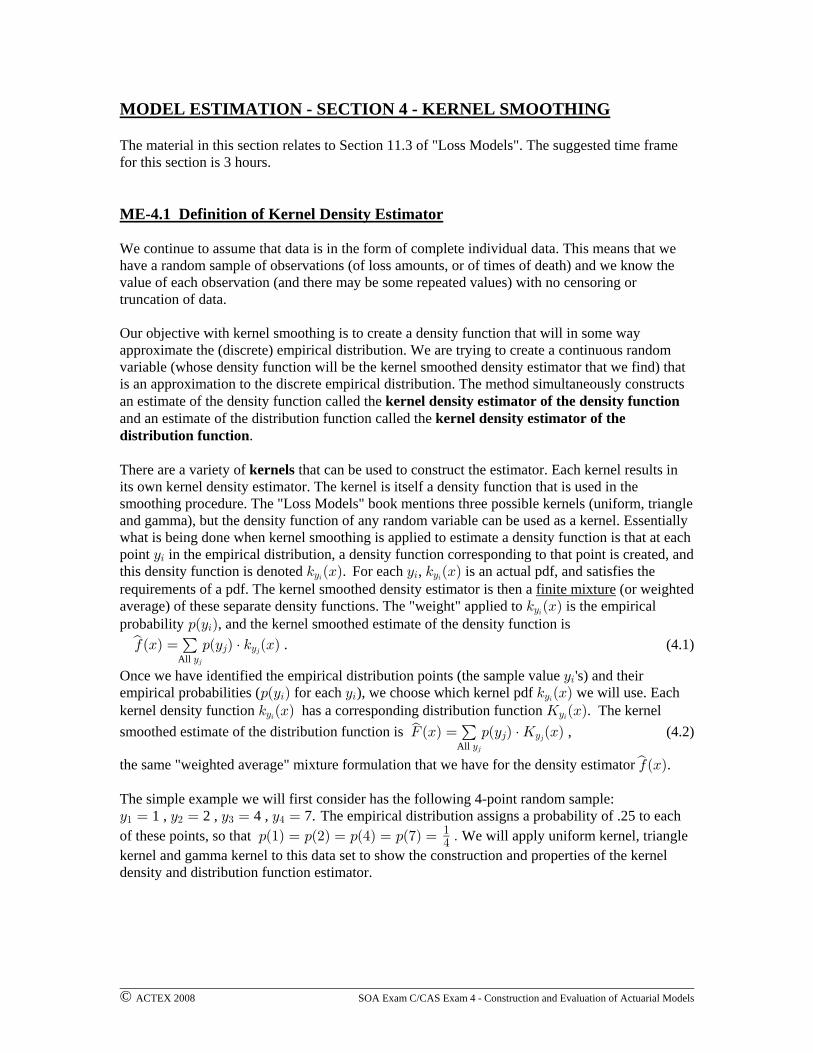
We continue to assume that data is in the form of complete individual data. This means that wehave a random sample of observations (of loss amounts, or of times of death) and we know thevalue of each observation (and there may be some repeated values) with no censoring ortruncation of data.
Our objective with kernel smoothing is to create a density function that will in some wayapproximate the (discrete) empirical distribution. We are trying to create a continuous randomvariable (whose density function will be the kernel smoothed density estimator that we find) thatis an approximation to the discrete empirical distribution. The method simultaneously constructsan estimate of the density function called the kernel density estimator of the density functionand an estimate of the distribution function called the kernel density estimator of thedistribution function.
There are a variety of that can be used to construct the estimator. Each kernel results inkernelsits own kernel density estimator. The kernel is itself a density function that is used in thesmoothing procedure. The "Loss Models" book mentions three possible kernels (uniform, triangleand gamma), but the density function of any random variable can be used as a kernel. Essentiallywhat is being done when kernel smoothing is applied to estimate a density function is that at eachpoint in the empirical distribution, a density function corresponding to that point is created, andC3this density function is denoted . For each , is an actual pdf, and satisfies the5 ÐBÑ C 5 ÐBÑC 3 C3 3
requirements of a pdf. The kernel smoothed density estimator is then a (or weightedfinite mixtureaverage) of these separate density functions. The "weight" applied to is the empirical5 ÐBÑC3
probability , and the kernel smoothed estimate of the density function is:ÐC Ñ3
. (4.1)0ÐBÑ œ :ÐC Ñ † 5 ÐBÑsAll C
4 C4
4
Once we have identified the empirical distribution points (the sample value 's) and theirC3empirical probabilities ( for each ), we choose which kernel pdf we will use. Each:ÐC Ñ C 5 ÐBÑ3 3 C3
kernel density function has a corresponding distribution function . The kernel5 ÐBÑ O ÐBÑC C3 3
smoothed estimate of the distribution function is , (4.2)JÐBÑ œ :ÐC Ñ † O ÐBÑsAll C
4 C4
4
the same "weighted average" mixture formulation that we have for the density estimator .0ÐBÑs
The simple example we will first consider has the following 4-point random sample:C œ C œ C œ C œ" # $ %1 , 2 , 4 , 7. The empirical distribution assigns a probability of .25 to eachof these points, so that We will apply uniform kernel, triangle:Ð"Ñ œ :Ð#Ñ œ :Ð%Ñ œ :Ð(Ñ œ Þ"
%kernel and gamma kernel to this data set to show the construction and properties of the kerneldensity and distribution function estimator.

© ACTEX 2008 SOA Exam C/CAS Exam 4 - Construction and Evaluation of Actuarial Models
According to the definition of , the way in which we calculate , is to apply the formula0ÐBÑ 0ÐBÑs s
. For our example, we have ,0ÐBÑ œ :ÐC Ñ † 5 ÐBÑ C œ " ß C œ # ß C œ % ß C œ (sAll C
4 C " # $ %4
4
and . Then ,:Ð"Ñ œ :Ð#Ñ œ :Ð%Ñ œ :Ð(Ñ œ Þ#& 0ÐBÑ œ ÐÞ#&ÑÒ5 ÐBÑ 5 ÐBÑ 5 ÐBÑ 5 ÐBÑÓs" # % (
where the functions are the kernel density functions, and5 ÐBÑC
J ÐBÑ œ ÐÞ#&ÑÒO ÐBÑ O ÐBÑ O ÐBÑ O ÐBÑÓs " # % ( .Note that the subscript of and is the -value. For instance, is the kernel function5 O C 5 ÐBÑ3 %
associated with the 3rd -value, ( is not the 4-th kernel pdf).C C œ % 5 ÐBÑ$ %
ME-4.2 Uniform Kernel Estimator
Uniform kernel density estimator with bandwidth 0ÐBÑ ,s
One of the kernels introduced in the "Loss Models" book is the uniform kernel withbandwidth ., The uniform kernel is based on the continuous uniform distribution. Recall that
the uniform distribution on the interval has pdf . (4.3)for otherwise
Ò-ß .Ó 5ÐBÑ œ- Ÿ B Ÿ .
!œ "
.-
For the uniform kernel with bandwidth , at each sample point , the kernel density is the, C 5 ÐBÑ3 C3
density function for the uniform distribution on the interval , so thatÒC , ß C ,Ó3 3
. (4.4)for otherwise
5 ÐBÑ œC , Ÿ B Ÿ C ,
!C
3 33 œ "
#,
The graph of is a horizontal line of height on the interval , and it is 05 ÐBÑ ÒC , ß C ,ÓC 3 33
"#,
outside that interval; the graph is a rectangle with an area of 1 (since is a pdf, total area5 ÐBÑC3
must be 1).
We will illustrate this method by applying the uniform kernel with a bandwidth of .4 (a somewhatarbitrary choice). At each of the original data points we create a rectangle, with the sample datapoint value at the center of the base of the rectangle, and with the area of the rectangle being 1.For sample data point in the original random sample, we create a rectangle whose base is fromC3C , C ,3 3 to , and whose height is chosen so that the area of the rectangle is 1. Since the baseis , the height must be . With our chosen value of , the rectangles will all have height#, , œ Þ%"
#,"
#ÐÞ%Ñ œ "Þ#& , and there will be four rectangles with the following bases, .ÒÞ' ß "Þ%Ó ß Ò"Þ' ß #Þ%Ó ß Ò$Þ' ß %Þ%Ó ß Ò'Þ' ß (Þ%Ó
The notation , , and describes the four "straight-line" functions5 ÐBÑ 5 ÐBÑ 5 ÐBÑ 5 ÐBÑ" # % (
represented in the graph below (note that the subscript of is the -value for the -th interval).5 C 5For instance, for , and for any outside the interval5 ÐBÑ œ "Þ#& Þ' Ÿ B Ÿ "Þ% 5 ÐBÑ œ ! B" "
ÒÞ' ß "Þ%Ó 5 . Similar conditions apply to the other three rectangles. The subscript to is the value ofthe data point from the original random sample. This identifies which rectangle is beingconsidered. Note that for each sample data point , is the pdf of the uniform distribution onC 5 ÐBÑC
the interval from to .C , C ,
What we have created is four separate uniform distributions, one for each interval. The graph ofthese four rectangles is as follows.

© ACTEX 2008 SOA Exam C/CAS Exam 4 - Construction and Evaluation of Actuarial Models
The way in which we apply the formula is as follows.0ÐBÑ œ :ÐC Ñ † 5 ÐBÑsAll C
4 C4
4
Given a value of , in order to find , we first determine which rectangle bases contain . WeB 0ÐBÑ Bs
only need to know the rectangles for which is in the base because for values of B 5 ÐBÑ œ ! BC
that are outside of the base rectangle around . We then find the value for each rectangleC 5ÐBÑand multiply by the empirical probability for that rectangle's base center point.
For instance, suppose we wish to find the kernel density estimator at , i.e., we wish toB œ "Þ"
find . is found by first identifying which rectangle bases contain the value 1.1. We0Ð"Þ"Ñ 0Ð"Þ"Ñs s
see that 1.1 is in the interval , so only the kernel function will be non-zero inÒÞ' ß "Þ%Ó 5 ÐBÑ"
calculating ( since 1.1 is not in the interval centered at ,0Ð"Þ"Ñ 5 Ð"Þ"Ñ œ ! Ò"Þ' ß #Þ%Ó C œ #s# #
and the same applies to and ).C œ % C œ ($ %
We find by multiplying the empirical probability of for the data point 10Ð"Þ"Ñ :Ð"Ñ œ Þ#& C œs"
by ( is the sample data point for which the rectangle with base was5 Ð"Þ"Ñ C œ " ÒÞ' ß "Þ%Ó" "
constructed, and is the value of the kernel function at point at which we are finding the5 Ð"Þ"Ñ"
density). Since for any in the interval , it follows that 5 ÐBÑ œ "Þ#& B ÒÞ' ß "Þ%Ó 5 Ð"Þ"Ñ œ "Þ#&" "
and . Writing out the full expression for we get0Ð"Þ"Ñ œ ÐÞ#&ÑÐ"Þ#&Ñ œ Þ$"#& 0Ð"Þ"Ñs s
0Ð"Þ"Ñ œ :ÐC Ñ † 5 Ð"Þ"Ñ œ ÐÞ#&Ñ5 Ð"Þ"Ñ ÐÞ#&Ñ5 Ð"Þ"Ñ ÐÞ#&Ñ5 Ð"Þ"Ñ ÐÞ#&Ñ5 Ð"Þ"ÑsAll C
4 C " # % (4
4
œ ÐÞ#&ÑÐ"Þ#&Ñ ÐÞ#&ÑÐ!Ñ ÐÞ#&ÑÐ!Ñ ÐÞ#&ÑÐ!Ñ œ Þ$"#& Þ
Again, it is important to note that we only used since the value was only in the5 Ð"Þ"Ñ B œ "Þ""
first of the four intervals for the rectangle bases.
Suppose we consider the -value and we wish to find , the kernel densityB B œ $Þ& 0Ð$Þ&Ñs
estimator at . We see that is not in any of the four intervals formed by the basesB œ $Þ& B œ $Þ&
of the four rectangles. Therefore, , since for each sample data point .0Ð$Þ&Ñ œ ! 5 Ð$Þ&Ñ œ ! CsC 33
Note that in the simple example we are now considering, since each is in either one rectangleB
base or none, will be .3125 if is in one of the four rectangle bases, and if is0ÐBÑ B 0ÐBÑ œ ! Bs s
not in any of the four rectangle bases.
© ACTEX 2008 SOA Exam C/CAS Exam 4 - Construction and Evaluation of Actuarial Models
If we were to draw the graph of this it would look the same as the four rectangles in the0ÐBÑs
graph above, but the heights would be .3125 instead of 1 for each rectangle.
If the rectangle bases are wider (if the bandwidth is increased), some bases may overlap and someB B's will be in two or more rectangle bases. If that is the case, then for that , in the relationship0ÐBÑ œ :ÐC Ñ † 5 ÐBÑ 5 ÐBÑs
All C4 C C
4
4 4 , more than one will be non-zero.
The following variation on the example considers this.
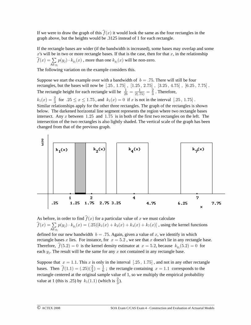
Suppose we start the example over with a bandwidth of . There will still be four, œ Þ(&rectangles, but the bases will now be .ÒÞ#& ß "Þ(&Ó ß Ò"Þ#& ß #Þ(&Ó ß Ò$Þ#& ß %Þ(&Ó ß Ò'Þ#& ß (Þ(&Ó
The rectangle height for each rectangle will be . Therefore," " ##, #ÐÞ(&Ñ $œ œ
5 ÐBÑ œ Þ#& Ÿ B Ÿ "Þ(& 5 ÐBÑ œ ! B ÒÞ#& ß "Þ(&Ó" "#$ for , and if is not in the interval .
Similar relationships apply for the other three rectangles. The graph of the rectangles is shownbelow. The darkened horizontal line segment represents the region where two rectangle basesintersect. Any between and is in both of the first two rectangles on the left. TheB "Þ#& "Þ(&intersection of the two rectangles is also lightly shaded. The vertical scale of the graph has beenchanged from that of the previous graph.
As before, in order to find for a particular value of we must calculate0ÐBÑ Bs
0ÐBÑ œ :ÐC Ñ † 5 ÐBÑ œ ÐÞ#&ÑÒ5 ÐBÑ 5 ÐBÑ 5 ÐBÑ 5 ÐBÑÓsAll C
4 C " # % (4
4 , using the kernel functions
defined for our new bandwidth . Again, given a value of , we identify in which, œ Þ(& Brectangle bases lies. For instance, for , we see that doesn't lie in any rectangle base.B B œ &Þ# B
Therefore, is the kernel density estimator at , because for0Ð&Þ#Ñ œ ! B œ &Þ# 5 Ð&Þ#Ñ œ !sC4
each . The result will be the same for any not contained in any rectangle base.C B4
Suppose that . This is only in the interval , and not in any other rectangleB œ "Þ" B ÒÞ#& ß "Þ(&Ó
bases. Then ; the rectangle containing corresponds to the0Ð"Þ"Ñ œ ÐÞ#&ÑÐ Ñ œ B œ "Þ"s # "$ '
rectangle centered at the original sample value of 1, so we multiply the empirical probabilityvalue at 1 (this is .25) by (which is ).5 Ð"Þ"Ñ"
#$

© ACTEX 2008 SOA Exam C/CAS Exam 4 - Construction and Evaluation of Actuarial Models
Note that for in any of the following intervals:0ÐBÑ œ Bs "'
, or .Þ#& Ÿ B "Þ#& "Þ(& B Ÿ #Þ(& ß $Þ#& Ÿ B Ÿ %Þ(& 'Þ#& Ÿ B Ÿ (Þ(&This is because for in any of those regions, is in exactly one rectangle base.B B
Suppose that . Then is in two rectangle bases, those being andB œ "Þ% B ÒÞ#& ß "Þ(&Ó
Ò"Þ#& ß #Þ(&Ó 0Ð"Þ%Ñs . In order to find we must include a factor for each rectangle base thatcontains .B0Ð"Þ%Ñ œ ÐÞ#&ÑÒ5 Ð"Þ%Ñ 5 Ð"Þ%Ñ 5 Ð"Þ%Ñ 5 Ð"Þ%ÑÓ œ ÐÞ#&ÑÒ ! !Ó œs
" # % (# # "$ $ $ .
0ÐBÑ œ B "Þ#& Ÿ B Ÿ "Þ(& Bs "$ for any in the interval because those 's are in two intervals.
The complete graph of the kernel smoothed density estimator based on bandwidth .75 isillustrated below. It is found by combining the heights of the rectangles in any intervals for whichthey overlap. The following is the graph of the uniform kernel smoothed density estimator withbandwidth .75. As the bandwidth gets wider there will be more intersection regions and some 'sBmay be in several rectangle bases.
One other point to note about the uniform kernel is that if is an interval endpoint, either B C ,
or , then . for values outside the closed interval .C , 5 ÐBÑ œ 5 ÐBÑ œ ! B ÒC , ß C ,ÓC C"#,
Uniform kernel estimator of the distribution function, with bandwidth JÐBÑß ,s
We can apply kernel density estimation to estimate the distribution function .JÐBÑ œ T Ò\ Ÿ BÓThe algebraic expression for the kernel estimator of the distribution function is .JÐBÑ œ :ÐC Ñ † O ÐBÑs
All C4 C
4
4
For specific values of and , is the cdf for the kernel pdf ; is theB C O ÐBÑ 5 ÐBÑ O ÐBÑ4 C C C4 4 4
probability to the left of for the kernel distribution centered at .B C4
For the uniform kernel with bandwidth , the formal definition of is, O ÐBÑC4
. (4.5)O ÐBÑ œ
! B C ,
C , Ÿ B Ÿ C ,
" B C ,
CBC,
#,
Note that means that the rectangle base interval around is completely to the left of B C , C B(less than ), so the full rectangle area of 1 is used ( ), and means that theB O ÐBÑ œ " B C ,C
rectangle base area around is completely to the right of so that the interval can be ignoredC B( ); see the graphs below illustrating these points.O ÐBÑ œ !C
© ACTEX 2008 SOA Exam C/CAS Exam 4 - Construction and Evaluation of Actuarial Models
In order to find for a particular value of , we must determine which rectangle baseJÐBÑ Bs
intervals are completely to the left of , which are completely to the right of , and which containB B
B JÐBÑ :ÐC Ñ † O ÐBÑs. will be a sum of (possibly) several factors. What we trying to do is add4 C4
up the probability in the kernel density that is to the left of BÞ
For any rectangle base interval completely to the right of , we have and that term inB O ÐBÑ œ !C4
J ÐBÑ B Ÿ C , B , Ÿ Cs can be ignored. This will occur if , or equivalently, if .4 4
If a rectangle base interval is completely to the left of , and if that rectangle base is centered atBthe random sample point , then . This will occur if , or equivalently, ifC O ÐBÑ œ " C , Ÿ B4 C 44
C B ,4 .
If is inside the rectangle base interval for the random sample point thenB C4
O ÐBÑ œ ÒB ÐC ,ÑÓ œ ÒÐB ,Ñ C ÓC 4 44 Ð Ñ Ð Ñ" "#, #, . (4.6)
Note that is the area in the rectangle centered at that is to theB ÐC ,Ñ œ ÐB ,Ñ C C4 4 4
left of . This is illustrated in the graphs below.B
Once we have identified the value of for each , we can calculateO ÐBÑ CC 44
J ÐBÑ œ :ÐC Ñ † O ÐBÑsAll C
4 C4
4 .
For instance, suppose that we consider the bandwidth example above, and we wish to, œ Þ(&
find . We see (in the graphs below) that the rectangle base intervals andJÐ%Þ&Ñ ÒÞ#& ß "Þ(&Ós
Ò"Þ#& ß #Þ(&Ó B œ %Þ& O Ð%Þ&Ñ œ " O Ð%Þ&Ñ œ " are both completely to the left of , so and ." #
The point is inside the rectangle base interval , and the area in thatB œ %Þ& Ò$Þ#& ß %Þ(&Ó
rectangle to the left of is ;B œ %Þ& O Ð%Þ&Ñ œ ÒB ÐC ,ÑÓ œ Ð%Þ& $Þ#&ÑÐ Ñ œ Þ)$$$% 4 Ð Ñ" ##, $
note that we can also write this as .ÒÐB ,Ñ C Ó œ Ò%Þ& Þ(& %ÓÐ Ñ4 Ð Ñ" ##, $
Finally, is completely to the left of the rectangle base interval , so thatB œ %Þ& Ò'Þ#& ß (Þ#&Ó
O Ð%Þ&Ñ œ ! JÐ%Þ&Ñ œ ÐÞ#&ÑÐ"Ñ ÐÞ#&ÑÐ"Ñ ÐÞ#&ÑÐÞ)$$$Ñ ÐÞ#&ÑÐ!Ñ œ Þ(!)$s( . Therefore, .
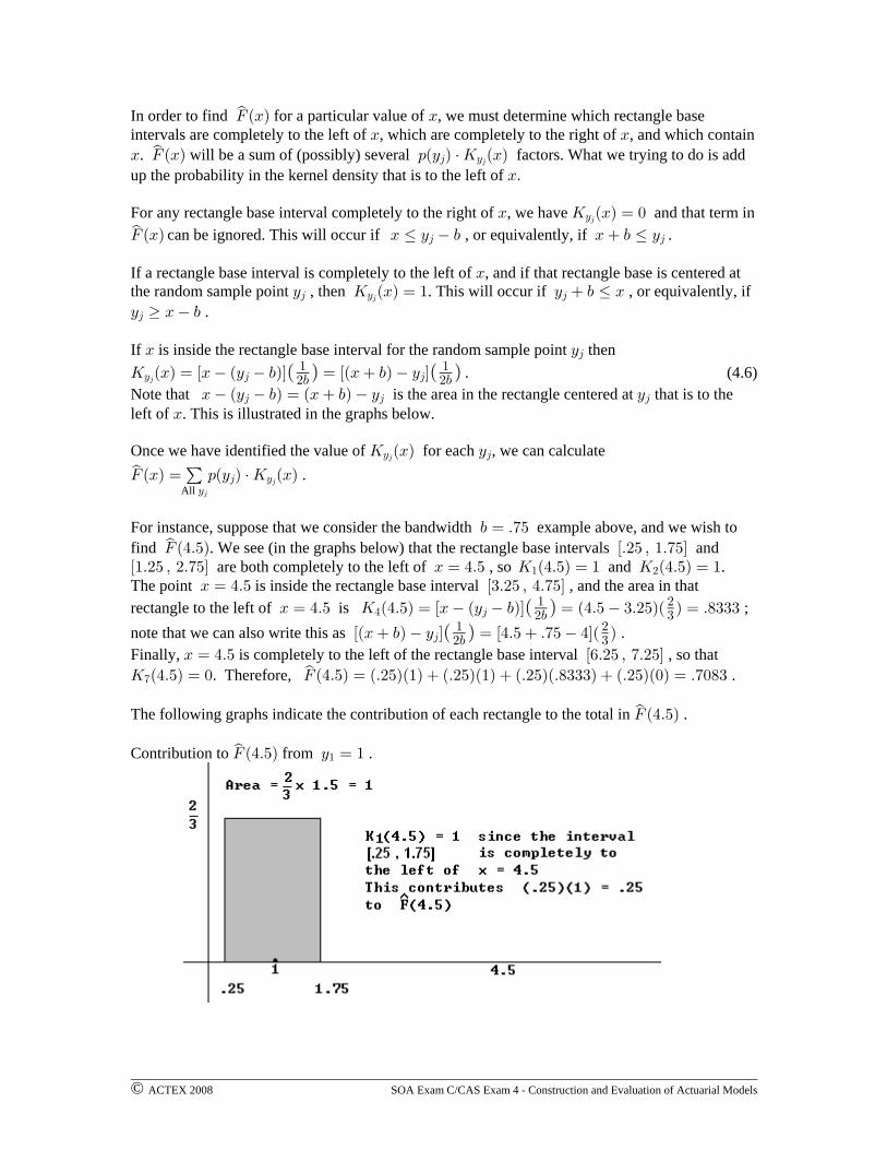
The following graphs indicate the contribution of each rectangle to the total in .JÐ%Þ&Ñs
Contribution to from .JÐ%Þ&Ñ C œ "s "

© ACTEX 2008 SOA Exam C/CAS Exam 4 - Construction and Evaluation of Actuarial Models
Contribution to from .JÐ%Þ&Ñ C œ #s #
Contribution to from .JÐ%Þ&Ñ C œ %s $
Contribution to from .JÐ%Þ&Ñ C œ (s %

© ACTEX 2008 SOA Exam C/CAS Exam 4 - Construction and Evaluation of Actuarial Models
As another example, suppose that we wish to find .JÐ"Þ%Ñs
To find we note that intervals and are both completely to theJÐ"Þ%Ñ Ò$Þ#& ß %Þ(&Ó Ò'Þ#& ß (Þ(&Ós
right, so they contribute nothing. We also see that is in the interval , so thatB œ "Þ% ÒÞ#& ß "Þ(&Ó
O Ð"Þ%Ñ œ Ð"Þ% Þ#&ÑÐ Ñ œ Ð"Þ% Þ(& "ÑÐ Ñ œ Þ(''("# #$ $ .
We see that is in the interval , so thatB œ "Þ% Ò"Þ#& ß #Þ(&Ó
O Ð"Þ%Ñ œ Ð"Þ% "Þ#&ÑÐ Ñ œ Ð"Þ% Þ(& #ÑÐ Ñ œ Þ"!!## #$ $ .
Therefore,JÐ"Þ%Ñ œ :Ð"ÑO Ð"Þ%Ñ :Ð#ÑO Ð"Þ%Ñ :Ð%ÑO Ð"Þ%Ñ :Ð(ÑO Ð"Þ%Ñs " # % (
œ ÐÞ#&ÑÐÞ(''(Ñ ÐÞ#&ÑÐÞ"!!Ñ ÐÞ#&ÑÐ!Ñ ÐÞ#&ÑÐ!Ñ œ Þ#"'( .
For the interval , , a straight line rising from 0 to 1 on theC , Ÿ B Ÿ C , O ÐBÑ œ4 4 C4BC,
#,
interval. If we carefully identify on each interval, we can plot the graph of .O ÐBÑ JÐBÑsC4
Using the example with bandwidth , we have, œ Þ)
J ÐBÑ œs
! B Þ#
ÐÞ#&Ñ œ Þ# Ÿ B Ÿ "Þ#
ÐÞ#&Ñ œ "Þ# Ÿ B Ÿ "Þ)
ÐÞ#&ÑÐ" œ "Þ) Ÿ B Ÿ #Þ)
ÐÞ#&ÑÐ
Ð Ñ
Ð Ñ
Ñ
B"Þ) BÞ#"Þ' 'Þ%
B"Þ) B#Þ) BÞ("Þ' "Þ' $Þ#B#Þ) BÞ%
"Þ' 'Þ%" "Ñ œ Þ& #Þ) Ÿ B Ÿ $Þ#
ÐÞ#&ÑÐ" " Ñ œ $Þ# Ÿ B Ÿ %Þ)
ÐÞ#&ÑÐ" " "Ñ œ Þ(& %Þ) Ÿ B Ÿ 'Þ#
ÐÞ#&ÑÐ" " " Ñ œ 'Þ# Ÿ B Ÿ (Þ)
ÐÞ#&ÑÐ" " " "
B%Þ) B"Þ' 'Þ%
B(Þ) B"Þ%"Þ' 'Þ%
Ñ œ " B (Þ)
The graph of is a series of line segments. The slope changes whenever crosses over anJÐBÑ Bs
interval endpoint, such as .2 , 1.2 , 1.8 , etc.
© ACTEX 2008 SOA Exam C/CAS Exam 4 - Construction and Evaluation of Actuarial Models
ME-4.3 The Triangle Kernel Estimator
Triangle kernel density estimator with bandwidth 0ÐBÑ ,s
The textbook mentions kernels other than the uniform. One of them is the . Thetriangle kernelprocedure is similar to that of the uniform kernel, the difference being that the rectangleconstructed around each is replaced by an isosceles triangle which has at the center of theC C4 4
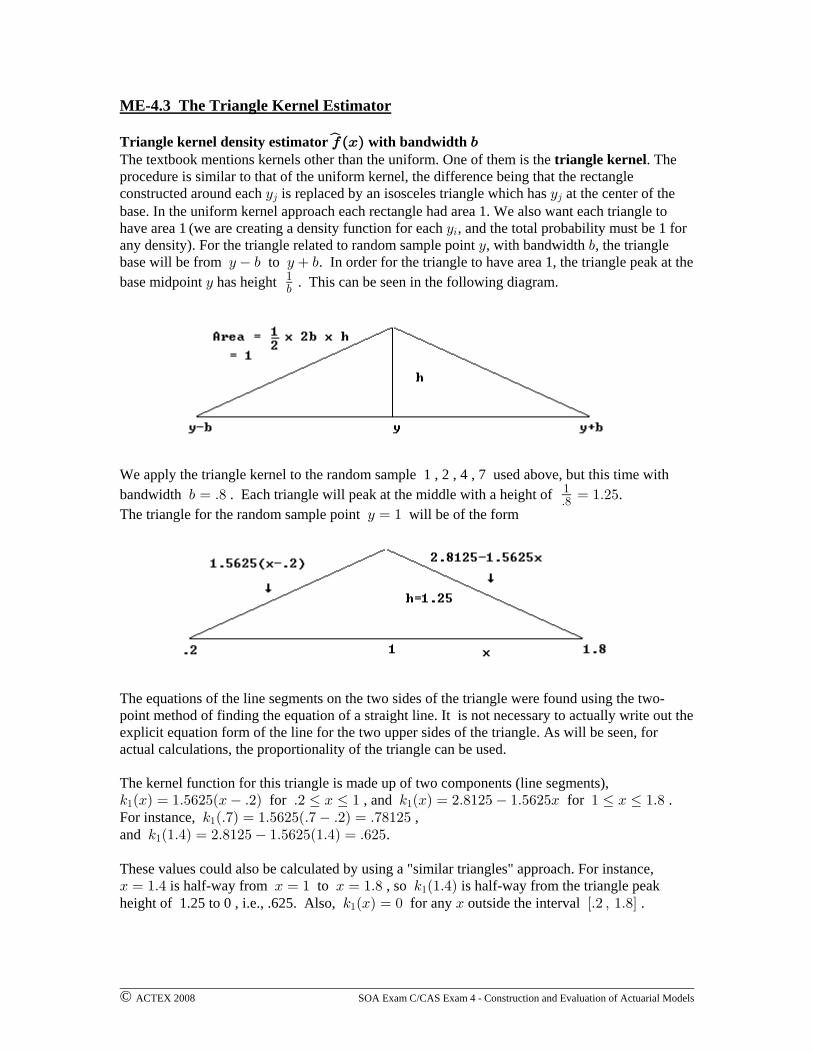
base. In the uniform kernel approach each rectangle had area 1. We also want each triangle tohave area 1 (we are creating a density function for each , and the total probability must be 1 forC3any density). For the triangle related to random sample point , with bandwidth , the triangleC ,base will be from to . In order for the triangle to have area 1, the triangle peak at theC , C ,
base midpoint has height . This can be seen in the following diagram.C ",
We apply the triangle kernel to the random sample 1 , 2 , 4 , 7 used above, but this time withbandwidth . Each triangle will peak at the middle with a height of ., œ Þ) œ "Þ#&"
Þ)The triangle for the random sample point will be of the formC œ "
The equations of the line segments on the two sides of the triangle were found using the two-point method of finding the equation of a straight line. It is not necessary to actually write out theexplicit equation form of the line for the two upper sides of the triangle. As will be seen, foractual calculations, the proportionality of the triangle can be used.
The kernel function for this triangle is made up of two components (line segments),5 ÐBÑ œ "Þ&'#&ÐB Þ#Ñ Þ# Ÿ B Ÿ " 5 ÐBÑ œ #Þ)"#& "Þ&'#&B " Ÿ B Ÿ "Þ)" " for , and for .For instance, ,5 ÐÞ(Ñ œ "Þ&'#&ÐÞ( Þ#Ñ œ Þ()"#&"
and .5 Ð"Þ%Ñ œ #Þ)"#& "Þ&'#&Ð"Þ%Ñ œ Þ'#&"
These values could also be calculated by using a "similar triangles" approach. For instance,B œ "Þ% B œ " B œ "Þ) 5 Ð"Þ%Ñ is half-way from to , so is half-way from the triangle peak"
height of 1.25 to 0 , i.e., .625. Also, for any outside the interval .5 ÐBÑ œ ! B ÒÞ# ß "Þ)Ó"

© ACTEX 2008 SOA Exam C/CAS Exam 4 - Construction and Evaluation of Actuarial Models
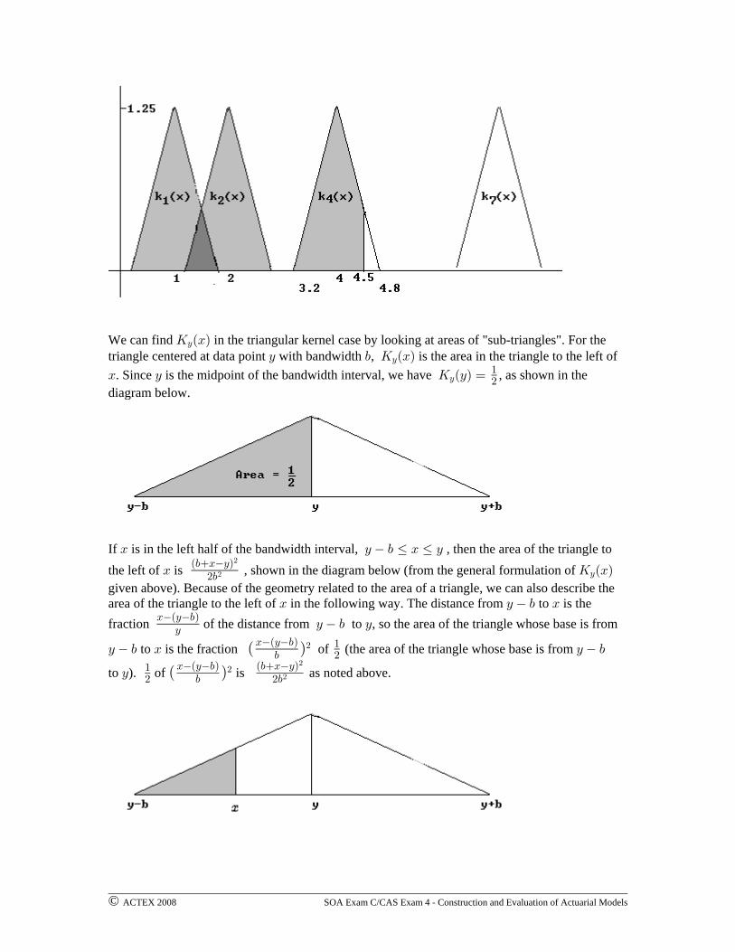
We construct triangle kernel functions for each of the original -values in the random sample.CThe graphs of all the triangle kernel functions is as follows.
Suppose we wish to find . As in the uniform kernel approach, we first find which triangle0Ð%Þ&Ñs
base intervals contain the point . We see that only the base interval for , which isB œ %Þ& 5 ÐBÑ%
Ò$Þ# ß %Þ)Ó B œ %Þ&contains . To calculate the smoothed estimate, the same relationship applies forthe triangle kernel, .0ÐBÑ œ :ÐC Ñ † 5 ÐBÑs
All C4 C
4
4
In this example (since is not in the triangle base5 Ð%Þ&Ñ œ 5 Ð%Þ&Ñ œ 5 Ð%Þ&Ñ œ ! B œ %Þ&" # (
interval for those kernel functions). Therefore, . From the empirical0Ð%Þ&Ñ œ :Ð%Ñ † 5 Ð%Þ&Ñs%
distribution we know that . Since is of the way from to ,:Ð%Ñ œ Þ#& B œ %Þ& B œ % B œ %Þ)&)
there is of the way left to go, and since the triangle drops from a height of 1.25 to 0 as goes$) B
from 4 to 4.8 , we see that . Then5 Ð%Þ&Ñ œ ‚ "Þ#& œ Þ%')(&%$)
0Ð%Þ&Ñ œ ÐÞ#&ÑÐÞ%')(&Ñ œ Þ""(")(&s .
Suppose that we wish to find . We see that lies in two triangle base intervals,0Ð"Þ%Ñ B œ "Þ%s
for on and for on .5 ÐBÑ ÒÞ# ß "Þ)Ó 5 ÐBÑ Ò"Þ# ß #Þ)Ó" #
Then (there is no contribution from or since0Ð"Þ%Ñ œ Þ#& ‚ 5 Ð"Þ%Ñ Þ#& ‚ 5 Ð"Þ%Ñ 5 5s" # % (
B œ "Þ% is not in the corresponding intervals).
Since is half-way between and (the base interval for ) , we see fromB œ "Þ% B œ " B œ "Þ) 5"the geometry of the diagram above that (the upper "dot" in the5 Ð"Þ%Ñ œ ‚ "Þ#& œ Þ'#&"
"#
diagram above). Since is one-quarter of the way from to (the baseB œ "Þ% B œ "Þ# B œ #
interval for ) , we see that (the lower "dot" above) .5 5 Ð"Þ%Ñ œ ‚ "Þ#& œ Þ$"#&# #"%
Then .0Ð"Þ%Ñ œ ÐÞ#&ÑÐÞ'#&Ñ ÐÞ#&ÑÐÞ$"#&Ñ œ Þ#$%$(&s
We could have set up the algebraic form of the line segments in the various triangles.For instance, for , so that5 ÐBÑ œ #Þ)"#& "Þ&'#&B " Ÿ B Ÿ "Þ)"
5 Ð"Þ%Ñ œ #Þ)"#& "Þ&'#&Ð"Þ%Ñ œ Þ'#&" (as we have already seen).Also, for , so that 5 ÐBÑ œ "Þ&'#&ÐB "Þ#Ñ "Þ# Ÿ B Ÿ # 5 Ð"Þ%Ñ œ "Þ&'#&ÐÞ#Ñ œ Þ$"#& Þ# #

© ACTEX 2008 SOA Exam C/CAS Exam 4 - Construction and Evaluation of Actuarial Models
The algebraic form of the triangle kernel is . (4.7)5 ÐBÑ œ
! B C ,
C , Ÿ B Ÿ C
C Ÿ B Ÿ C ,
! B C ,
C
,BC,
,CB,
#
#
For instance, in the example just considered,
5 ÐBÑ œ
! B " Þ) œ Þ#
œ "Þ&'#&ÐB Þ#Ñ " Þ) œ Þ# Ÿ B Ÿ "
œ #Þ)"#& "Þ&'#&B " Ÿ B Ÿ "Þ) œ " Þ)
! B "Þ) œ " Þ)
"
Þ)B"Þ)
Þ)"BÞ)
#
#
. (4.8)
This gives the algebraic form of the two sides of the triangle for in the graph above.5 ÐBÑ"
The other kernel functions can be formulated in a similar way.
Triangle kernel estimator of the distribution function, with bandwidth JÐBÑß ,s
It is also possible to find the kernel density estimator of the distribution function using the
triangle kernel. We can use the form , (4.9)O ÐBÑ œ
! B C ,
C , Ÿ B Ÿ C
" C Ÿ B Ÿ C ,
" B C ,
C
Ð,BCÑ#,Ð,CBÑ
#,
#
#
#
#
and, as before, .JÐBÑ œ :ÐC Ñ † O ÐBÑsAll C
4 C4
4
Again, what we are really doing is finding the area to left of in each triangle, and we multiplyBthis area by for that rectangle.:ÐCÑ
For instance, the kernel smoothed estimate of would beJÐ%Þ&Ñ
J Ð%Þ&Ñ œ :Ð"ÑO Ð%Þ&Ñ :Ð#ÑO Ð%Þ&Ñ :Ð%ÑO Ð%Þ&Ñ :Ð(ÑO Ð%Þ&Ñs " # % ( .Since the triangle base centered at is completely to the left of 4.5, we have ,C œ " O Ð%Þ&Ñ œ "" "
and the same is true for , so that . Since the triangle base centered at C œ # O Ð%Þ&Ñ œ " C œ (# %2is completely to the right of 4.5, we have . is inside the interval centered atO Ð%Þ&Ñ œ ! B œ %Þ&(
C œ % C œ %$ $. The area to the left of 4.5 in the triangle centered at isO Ð%Þ&Ñ œ " C œ %% $(area to the right of 4.5 in the triangle centered at ).But [area to the right of 4.5 in the triangle centered at ] is equal toC œ %$" "# #‚ 5 Ð%Þ&Ñ ‚ Ð%Þ) %Þ&Ñ œ ‚ ÐÞ%')(&Ñ ‚ Ð%Þ) %Þ&Ñ œ Þ!(!$"#&% .Therefore, .O Ð%Þ&Ñ œ " Þ!(!$"#& œ Þ*#*')(&%
Alternatively, using Equation 4.9, we have .O Ð%Þ&Ñ œ " œ Þ*#*')(&%ÐÞ)%%Þ&Ñ
#ÐÞ)Ñ
#
#
Finally, JÐ%Þ&Ñ œ :Ð"ÑO Ð%Þ&Ñ :Ð#ÑO Ð%Þ&Ñ :Ð%ÑO Ð%Þ&Ñ :Ð(ÑO Ð%Þ&Ñs " # % (
œ ÐÞ#&ÑÐ"Ñ ÐÞ#&ÑÐ"Ñ ÐÞ#&ÑÐÞ*#*')(&Ñ ÐÞ#&ÑÐ!Ñ œ Þ($#%Þ
The shaded regions below are the areas that represent . The extra shading indicates thatO Ð%Þ&ÑC
this region is in both triangles.
© ACTEX 2008 SOA Exam C/CAS Exam 4 - Construction and Evaluation of Actuarial Models
We can find in the triangular kernel case by looking at areas of "sub-triangles". For theO ÐBÑC
triangle centered at data point with bandwidth , is the area in the triangle to the left ofC , O ÐBÑC
B C O ÐCÑ œ. Since is the midpoint of the bandwidth interval, we have , as shown in theC"#
diagram below.
If is in the left half of the bandwidth interval, , then the area of the triangle toB C , Ÿ B Ÿ C
the left of is , shown in the diagram below (from the general formulation of B O ÐBÑÐ,BCÑ
#,
#
# C
given above). Because of the geometry related to the area of a triangle, we can also describe thearea of the triangle to the left of in the following way. The distance from to is theB C , B
fraction of the distance from to , so the area of the triangle whose base is fromBÐC,ÑC C , C
C , B C , to is the fraction of (the area of the triangle whose base is from Ð ÑBÐC,Ñ, #
"#
to ). of is as noted above.C "# , #,
BÐC,Ñ Ð,BCÑÐ Ñ##
#

© ACTEX 2008 SOA Exam C/CAS Exam 4 - Construction and Evaluation of Actuarial Models
If is in the right half of the bandwidth interval, then the area to the left of is the complementB Bof the area to the right of , from to the right side of the bandwidth interval . The base ofB B C ,
the triangle from to is the fraction of the base of the triangle from yo , soB C , C C ,C,B
,
the area of the triangle whose base is from to is . The area of the shadedB C , ‚Ð ÑC,B, #
"#
region in the triangle below is , which is , describedO ÐBÑ " ‚ œ " C#Ð ÑC,B
, # #," Ð,CBÑ#
#
in the general formulation of given above.O ÐBÑC
Applying this to the numerical example above, we can find . The bandwidth is . soO Ð%Þ&Ñ , œ Þ)%
the left side of the bandwidth interval is , and the right side is . The interval from% Þ) œ $Þ# %Þ)
4.5 to 4.8 is of the interval from 4 to 4.8, so the area of the unshaded triangle isÞ$ $Þ) )œ
Ð Ñ$ ") #
#%‚ œ Þ!(!$"#& O Ð%Þ&Ñ œ " Þ!(!$"#& œ Þ*#*')(& . The are of the shaded region is ,
as noted above.
A kernel smoothing method can be created using any continuous random variable pdf as a kernelfunction. In the textbook, the gamma distribution as also presented as a possible kernel (thetextbook also has an example with a Pareto kernel).
ME-4.4 The Gamma Kernel Estimator
The Gamma kernel with shape parameter and has kernel density functionα ) œCα
for . (4.10)5 ÐBÑ œ B !C
Ð Ñ /
B Ð Ñ
α α αBC
BÎC
> α
If , then , , which is an exponential distribution with mean .α œ " 5 ÐBÑ œ / B ! CCBÎC"
C

© ACTEX 2008 SOA Exam C/CAS Exam 4 - Construction and Evaluation of Actuarial Models
The Gamma kernel does not require choosing a bandwidth , but instead requires choosing the,shape parameter . The kernel density estimator of the pdf of would still beα \
, where the 's are the original random sample values.0ÐBÑ œ :ÐC Ñ † 5 ÐBÑ CsAll C
4 C 44
4
Note that with the gamma kernel is never 0 for . Also, is a finite mixture of5 ÐBÑ B ! 0ÐBÑsC4
gamma distributions, where the mixing weights are the empirical probabilities .:ÐC Ñ4
The motivation behind the kernel density estimator is to create a continuous density function thatapproximates the probabilities assigned in the empirical distribution of a random sample. Thegraphs on pages 319 to 321 of the textbook illustrate some density functions that result whenapplying kernel smoothing. The examples given in the textbook also give graphs of some kernelsmoothed density functions.
Example ME-7: For the data of Example ME-6, apply each of the following three kernels toobtain the kernel smoothed density estimates and .0Ð"!Ñ 0Ð#!Ñs s
(1) Uniform kernel with bandwidth 2.(2) Triangular kernel with bandwidth 2.(3) Gamma kernel with shape parameter .α œ "
Solution: The 8 data points are , each with empirical$ ß % ß ) ß "! ß "# ß ") ß ## ß $&
probability .")
(1) Uniform kernel. . Since the bandwidth is 2,0Ð"!Ñ œ Ð Ñ5 Ð"!Ñs4œ"
)
C") 4
5 Ð"!Ñ œ ! C œ $ß %ß ")ß ## $& 5 Ð"!Ñ œ œ C œ )ß "! "#C 4 C 44 4 for and , and for and ." "#, %
0Ð"!Ñ œ Ð ÑÐ Ñ œ Þ!*$(& Bs " " " ") % % % . Note that when is the endpoint of a base interval, it is
included as part of that interval (so, for instance, for the base interval is andC œ ) Ò' ß "!Ó4
B œ "! is regarded as being in the interval).
0Ð#!Ñ œ Ð Ñ5 Ð#!Ñ 5 Ð#!Ñ œ ! C œ $ß %ß )ß "!ß "# $& 5 Ð#!Ñ œs4œ"
)
C C 4 C" ") %4 4 4 , and for and , and for
C œ ") ## 0Ð#!Ñ œ Ð ÑÐ Ñ œ Þ!'#&s4 and . ." " "
) % %
(2) Triangular kernel. Same bandwidth as (1) so the 0's from part (1) are still 0's.5 Ð"!Ñ œ œ ! B œ "!)
#)"!## (for the interval centered at 8, the triangle height is 0 at , the right
end of the interval)ß 5 Ð"!Ñ œ œ œ ß 5 Ð"!Ñ œ œ ! Þ"! "##"!"! " " #"!"#
# , # ## #
0Ð"!Ñ œ Ð ÑÐ Ñ œ Þ!'#& 5 Ð#!Ñ œ œ ! ß 5 Ð#!Ñ œ œ ! Þ 0Ð#!Ñ œ !s s" " #")#! ##!##) # # # . .") ### #
(3) Gamma kernel, , (an exponential distribution).α œ " 5 ÐBÑ œ /CBÎC"
C
5 ÐBÑ œ / ß Þ Þ Þ ß 5 ÐBÑ œ /$ $&BÎ$ BÎ$&" "
$ $& .0Ð"!Ñ œ Ð ÑÒ / / â / Ó œ Þ!#(*s " " " "
) $ % $&"!Î$ "!Î% "!Î$& .
0Ð#!Ñ œ Ð ÑÒ / / â / Ó œ Þ!"")s " " " ") $ % $&
#!Î$ #!Î% #!Î$& .
© ACTEX 2008 SOA Exam C/CAS Exam 4 - Construction and Evaluation of Actuarial Models
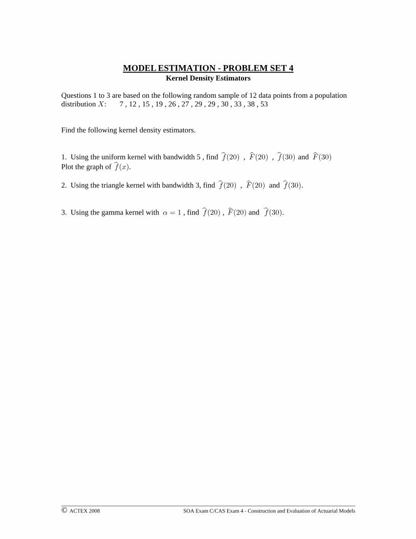
MODEL ESTIMATION - PROBLEM SET 4Kernel Density Estimators
Questions 1 to 3 are based on the following random sample of 12 data points from a populationdistribution : 7 , 12 , 15 , 19 , 26 , 27 , 29 , 29 , 30 , 33 , 38 , 53\
Find the following kernel density estimators.
1. Using the uniform kernel with bandwidth 5 , find , , and 0Ð#!Ñ J Ð#!Ñ 0Ð$!Ñ J Ð$!Ñs ss s
Plot the graph of .0ÐBÑs
2. Using the triangle kernel with bandwidth 3, find , and .0Ð#!Ñ J Ð#!Ñ 0Ð$!Ñs ss
3. Using the gamma kernel with , find , and .α œ " 0Ð#!Ñ J Ð#!Ñ 0Ð$!Ñs ss
© ACTEX 2008 SOA Exam C/CAS Exam 4 - Construction and Evaluation of Actuarial Models
MODEL ESTIMATION - PROBLEM SET 4 SOLUTIONS
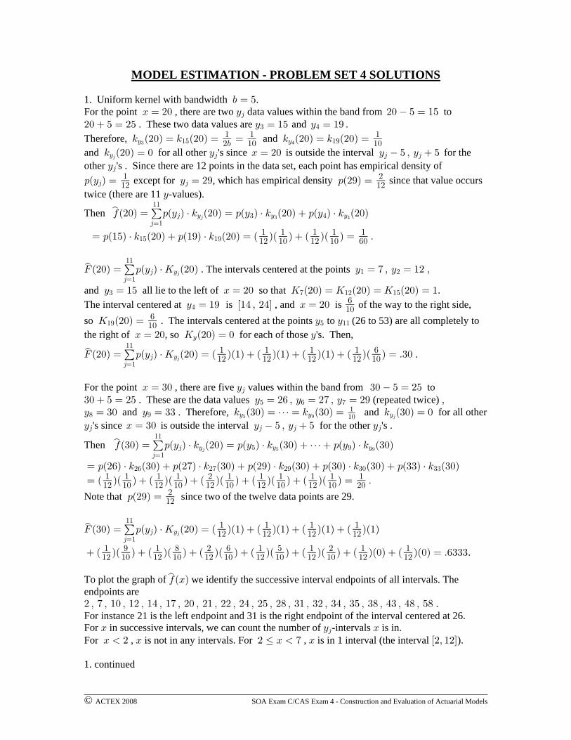
1. Uniform kernel with bandwidth ., œ &For the point , there are two data values within the band from toB œ #! C #! & œ "&4
#! & œ #& C œ "& C œ "* . These two data values are and .$ %
Therefore, and 5 Ð#!Ñ œ 5 Ð#!Ñ œ œ 5 Ð#!Ñ œ 5 Ð#!Ñ œC "& C "$
" " "#, "! "!4 9
and for all other 's since is outside the interval for the5 Ð#!Ñ œ ! C B œ #! C & ß C &C 4 4 44
other 's . Since there are 12 points in the data set, each point has empirical density ofC4
:ÐC Ñ œ C œ #* :Ð#*Ñ œ4 4" #"# "# except for , which has empirical density since that value occurs
twice (there are 11 -values).C
Then 0Ð#!Ñ œ :ÐC Ñ † 5 Ð#!Ñ œ :ÐC Ñ † 5 Ð#!Ñ :ÐC Ñ † 5 Ð#!Ñs4œ"
""
4 C $ C % C4 $ %
œ :Ð"&Ñ † 5 Ð#!Ñ :Ð"*Ñ † 5 Ð#!Ñ œ Ð ÑÐ Ñ Ð ÑÐ Ñ œ Þ"& "*" " " " ""# "! "# "! '!
J Ð#!Ñ œ :ÐC Ñ † O Ð#!Ñ C œ ( ß C œ "# ßs4œ"
""
4 C " #4 . The intervals centered at the points
and all lie to the left of so that .C œ "& B œ #! O Ð#!Ñ œ O Ð#!Ñ œ O Ð#!Ñ œ "$ ( "# "&
The interval centered at is , and is of the way to the right side,C œ "* Ò"% ß #%Ó B œ #!%'"!
so . The intervals centered at the points to (26 to 53) are all completely toO Ð#!Ñ œ C C"* & ""'"!
the right of , so for each of those 's. Then,B œ #! O Ð#!Ñ œ ! CC
J Ð#!Ñ œ :ÐC Ñ † O Ð#!Ñ œ Ð ÑÐ"Ñ Ð ÑÐ"Ñ Ð ÑÐ"Ñ Ð ÑÐ Ñ œ Þ$!s4œ"
""
4 C4" " " " '"# "# "# "# "! .
For the point , there are five values within the band from toB œ $! C $! & œ #&4
$! & œ #& C œ #' ß C œ #( ß C œ #* ß . These are the data values (repeated twice) & ' (
C œ $! C œ $$ 5 Ð$!Ñ œ â œ 5 Ð$!Ñ œ 5 Ð$!Ñ œ !) * C C C""! and . Therefore, and for all other& * 4
C B œ $! C & ß C & C4 4 4 4's since is outside the interval for the other 's .
Then 0Ð$!Ñ œ :ÐC Ñ † 5 Ð#!Ñ œ :ÐC Ñ † 5 Ð$!Ñ â :ÐC Ñ † 5 Ð$!Ñs4œ"
""
4 C & C * C4 & *
œ :Ð#'Ñ † 5 Ð$!Ñ :Ð#(Ñ † 5 Ð$!Ñ :Ð#*Ñ † 5 Ð$!Ñ :Ð$!Ñ † 5 Ð$!Ñ :Ð$$Ñ † 5 Ð$!Ñ#' #( #* $! $$
œ Ð ÑÐ Ñ Ð ÑÐ Ñ Ð ÑÐ Ñ Ð ÑÐ Ñ Ð ÑÐ Ñ œ Þ" " " " # " " " " " ""# "! "# "! "# "! "# "! "# "! #!
Note that since two of the twelve data points are 29.:Ð#*Ñ œ #"#
J Ð$!Ñ œ :ÐC Ñ † O Ð#!Ñ œ Ð ÑÐ"Ñ Ð ÑÐ"Ñ Ð ÑÐ"Ñ Ð ÑÐ"Ñs4œ"
""
4 C4" " " ""# "# "# "#
Ð ÑÐ Ñ Ð ÑÐ Ñ Ð ÑÐ Ñ Ð ÑÐ Ñ Ð ÑÐ Ñ Ð ÑÐ!Ñ Ð ÑÐ!Ñ œ Þ'$$$" * " ) # ' " & " # " ""# "! "# "! "# "! "# "! "# "! "# "# .
To plot the graph of we identify the successive interval endpoints of all intervals. The0ÐBÑs
endpoints are# ß ( ß "! ß "# ß "% ß "( ß #! ß #" ß ## ß #% ß #& ß #) ß $" ß $# ß $% ß $& ß $) ß %$ ß %) ß &) .For instance 21 is the left endpoint and 31 is the right endpoint of the interval centered at 26.For in successive intervals, we can count the number of -intervals is in.B C B4
For , is not in any intervals. For , is in 1 interval (the interval ).B # B # Ÿ B ( B Ò#ß "#Ó
1. continued

© ACTEX 2008 SOA Exam C/CAS Exam 4 - Construction and Evaluation of Actuarial Models
For , is in 2 intervals, etc. Since the sample point 29 occurs twice, its probability is( Ÿ B "! Bdoubled in the empirical distribution. Therefore, for instance, for , is in 5#& Ÿ B #) Bintervals; those intervals are (twice), and .Ò#"ß $"Ó ß Ò##ß $#Ó ß Ò#%ß $%Ó Ò#&ß $&Ó
To plot , we apply an empirical probability of to each sample point.0ÐBÑs ""#
0ÐBÑ œ ! B # 0ÐBÑ œ " ‚ œ # Ÿ B (s s for , for ," ""# "#
0ÐBÑ œ # ‚ œ ( B "! 0ÐBÑ œ & ‚ œ #& Ÿ B $$s s" " " &"# # "# "# for , . . . , for , . . .
2. Triangle kernel with bandwidth ., œ $For the point there is one value within the band from to 0 ;B œ #! C #! $ œ "( # $ œ #$4
this is the data value . Similar to the situation in part (a), we haveC œ "*%
5 Ð#!Ñ œ ! C C œ "* , œ $C 4 %4 for all except for . Using the triangle kernel with , and since
C œ "* Ÿ #! Ÿ ## œ C , 5 Ð#!Ñ œ œ œ% % C , we have %
,CB, * *
$"*#! ##
Alternatively, the height of each triangle is , and since is of the way from the" " ", $ $œ B œ #!
triangle base midpoint at 19 to the right of the triangle base at 22, is of the height of the5 Ð#!ÑC%#$
triangle, so . This is illustrated in the graph below.5 Ð#!Ñ œ ‚ œC%" # #$ $ *
Then .0Ð#!Ñ œ :ÐC Ñ † 5 Ð#!Ñ œ :ÐC Ñ † 5 Ð#!Ñ œ Ð ÑÐ Ñ œs4œ"
""
4 C % C4 %
" # ""# * &%
The intervals centered at points and all lie completely to the left ofC œ ( ß C œ "# ß C œ "&" $#
B œ #! O Ð#!Ñ œ O Ð#!Ñ œ O Ð#!Ñ œ " C, so that . For the 's from 26 to 53, the intervals all lie( "# "&
completely to the right of 20, so for each of them. From the triangle diagram above,O Ð#!Ñ œ !C
it can be seen that the area in the triangle to the right of 20 is , so that the area to# ‚ ‚ œ# " #* # *
the left of 20 in that triangle is Therefore,O Ð#!Ñ œ " œ Þ"*# (* *
J Ð#!Ñ œ Ð ÑÐ"Ñ Ð ÑÐ"Ñ Ð ÑÐ"Ñ Ð ÑÐ Ñ œs " " " " ( "("# "# "# "# * &% .
For the point there are four values within the band from to ; these areB œ $! C #( $$4
C œ #( ß C œ #* ß C œ $! C œ $$ 5 Ð$!Ñ œ !' ( ) * C (repeated twice) and . We have for all4
other -values. Since , we have (sinceC C œ #( Ÿ $! Ÿ $! œ C , 5 Ð$!Ñ œ œ !4 ' ' #($#($!
*B œ $! C œ #( is at the right end of the interval centered at ) ,'
since , we have ,C œ #* Ÿ $! Ÿ $# œ C , 5 Ð$!Ñ œ œ7 ( #*$#*$! #
* *
since , we have , andC , œ #( Ÿ $! Ÿ $! œ C 5 Ð$!Ñ œ œ) ) $!$$!$! "
* $since , we have (since is at the leftC , œ $! Ÿ $! Ÿ $$ œ C 5 Ð$!Ñ œ œ ! B œ $!* * $$
$$!$$*
end of the interval centered at ) C œ $$ Þ*
© ACTEX 2008 SOA Exam C/CAS Exam 4 - Construction and Evaluation of Actuarial Models
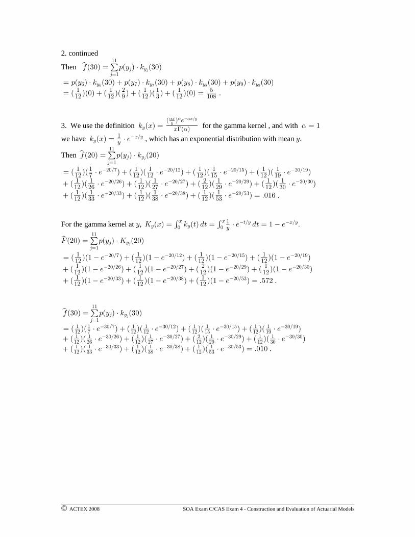
2. continued
Then 0Ð$!Ñ œ :ÐC Ñ † 5 Ð$!Ñs4œ"
""
4 C4
œ :ÐC Ñ † 5 Ð$!Ñ :ÐC Ñ † 5 Ð$!Ñ :ÐC Ñ † 5 Ð$!Ñ :ÐC Ñ † 5 Ð$!Ñ' C ( C ) C * C' ( ) *
œ Ð ÑÐ!Ñ Ð ÑÐ Ñ Ð ÑÐ Ñ Ð ÑÐ!Ñ œ" " # " " " &"# "# * "# $ "# "!) .
3. We use the definition for the gamma kernel , and with 5 ÐBÑ œ œ "C
Ð Ñ /
B Ð Ñ
α α αBC
BÎC
> α α
we have , which has an exponential distribution with mean .5 ÐBÑ œ † / CCBÎC"
C
Then 0Ð#!Ñ œ :ÐC Ñ † 5 Ð#!Ñs4œ"
""
4 C4
œ Ð ÑÐ † / Ñ Ð ÑÐ † / Ñ Ð ÑÐ † / Ñ Ð ÑÐ † / Ñ" " " " " " " ""# ( "# "# "# "& "# "*
#!Î( #!Î"# #!Î"& #!Î"*
Ð ÑÐ † / Ñ Ð ÑÐ † / Ñ Ð ÑÐ † / Ñ Ð ÑÐ † / Ñ" " " " # " " ""# #' "# #( "# #* "# $!
#!Î#' #!Î#( #!Î#* #!Î$!
Ð ÑÐ † / Ñ Ð ÑÐ † / Ñ Ð ÑÐ † / Ñ œ Þ!"'" " " " " ""# $$ "# $) "# &$
#!Î$$ #!Î$) #!Î&$ .
For the gamma kernel at , C O ÐBÑ œ 5 Ð>Ñ .> œ † / .> œ " / ÞC C! !
B B >ÎC BÎC' ' "C
J Ð#!Ñ œ :ÐC Ñ † O Ð#!Ñs4œ"
""
4 C4
œ Ð ÑÐ" / Ñ Ð ÑÐ" / Ñ Ð ÑÐ" / Ñ Ð ÑÐ" / Ñ" " " ""# "# "# "#
#!Î( #!Î"# #!Î"& #!Î"*
Ð ÑÐ" / Ñ Ð ÑÐ" / Ñ Ð ÑÐ" / Ñ Ð ÑÐ" / Ñ" " # ""# "# "# "#
#!Î#' #!Î#( #!Î#* #!Î$!
Ð ÑÐ" / Ñ Ð ÑÐ" / Ñ Ð ÑÐ" / Ñ œ Þ&(#" " ""# "# "#
#!Î$$ #!Î$) #!Î&$ .
0Ð$!Ñ œ :ÐC Ñ † 5 Ð$!Ñs4œ"
""
4 C4
œ Ð ÑÐ † / Ñ Ð ÑÐ † / Ñ Ð ÑÐ † / Ñ Ð ÑÐ † / Ñ" " " " " " " ""# ( "# "# "# "& "# "*
$!Î( $!Î"# $!Î"& $!Î"*
Ð ÑÐ † / Ñ Ð ÑÐ † / Ñ Ð ÑÐ † / Ñ Ð ÑÐ † / Ñ" " " " # " " ""# #' "# #( "# #* "# $!
$!Î#' $!Î#( $!Î#* $!Î$!
Ð ÑÐ † / Ñ Ð ÑÐ † / Ñ Ð ÑÐ † / Ñ œ Þ!"!" " " " " ""# $$ "# $) "# &$
$!Î$$ $!Î$) $!Î&$ .
Related Documents