EXCEL INTERMEDIATE - Revize

EXCEL INTERMEDIATE

Linda Muchow [email protected]

320-762-4539

1

Table of Contents IF Statement .......................................................................................................................................................................... 2

IF AND ................................................................................................................................................................................ 3

IFS ...................................................................................................................................................................................... 5

Nested IF Statement ......................................................................................................................................................... 6

Formula within IF Statement ............................................................................................................................................ 6

MAXIFS .............................................................................................................................................................................. 8

MINIFS ............................................................................................................................................................................... 8

IFERROR ................................................................................................................................................................................. 8

VLOOKUP ............................................................................................................................................................................. 10

Creating a Table .................................................................................................................................................................. 13

Add a Total Row .............................................................................................................................................................. 13

Convert to Normal Range ................................................................................................................................................ 14

Use a Table with VLOOKUP ............................................................................................................................................. 14

Date & Time Functions ........................................................................................................................................................ 14

Now & Today Functions .................................................................................................................................................. 14

YEARFAC .......................................................................................................................................................................... 15

NETWORKDAYS Function ................................................................................................................................................ 16

Workday Function ........................................................................................................................................................... 17

EDate ............................................................................................................................................................................... 18

EOMONTH ....................................................................................................................................................................... 19

Charting Tools ..................................................................................................................................................................... 19

Saving a Chart as a Template .......................................................................................................................................... 22

Create Charts with Keyboard Shortcuts .......................................................................................................................... 22

Custom Formats - Excel ....................................................................................................................................................... 29

Text Characters & Spacing .............................................................................................................................................. 29

Number Characters ......................................................................................................................................................... 30

Date Characters ............................................................................................................................................................... 31

Time Characters .............................................................................................................................................................. 31

2

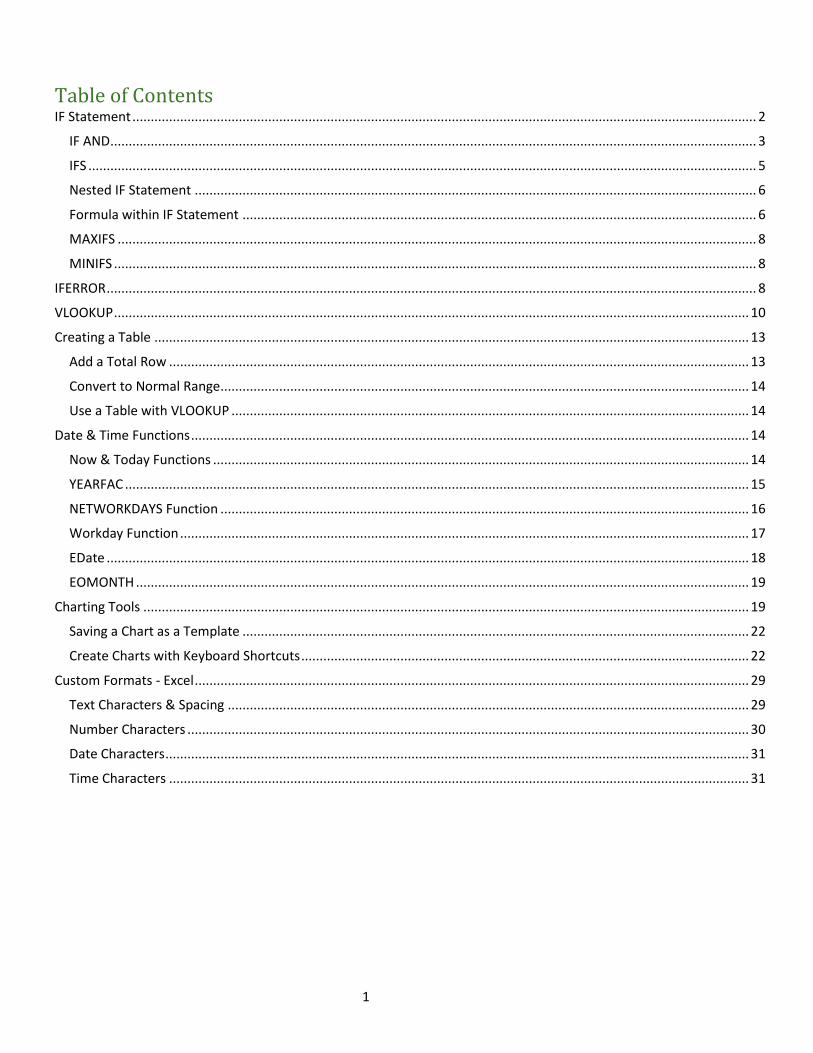
IF Statement The Excel IF Function returns one value if a specified condition evaluates to TRUE, or another value if it evaluates to FALSE. In this example, each employee received a Job rating with 1 being the worst rating and 5 being the best rating. Each employee that has a job rating of 4 or 5 will receive a $250 bonus. The IF function can run the logical reference (greater than 3) and put the number 250 in each cell that meets that requirement. If the job rating is less than 4, the IF statement will put a 0 in the cell.

1. From the Formulas Tab >> Function Library select Logical and then IF.

2. The Function Arguments window should be filled out as sown below.

3

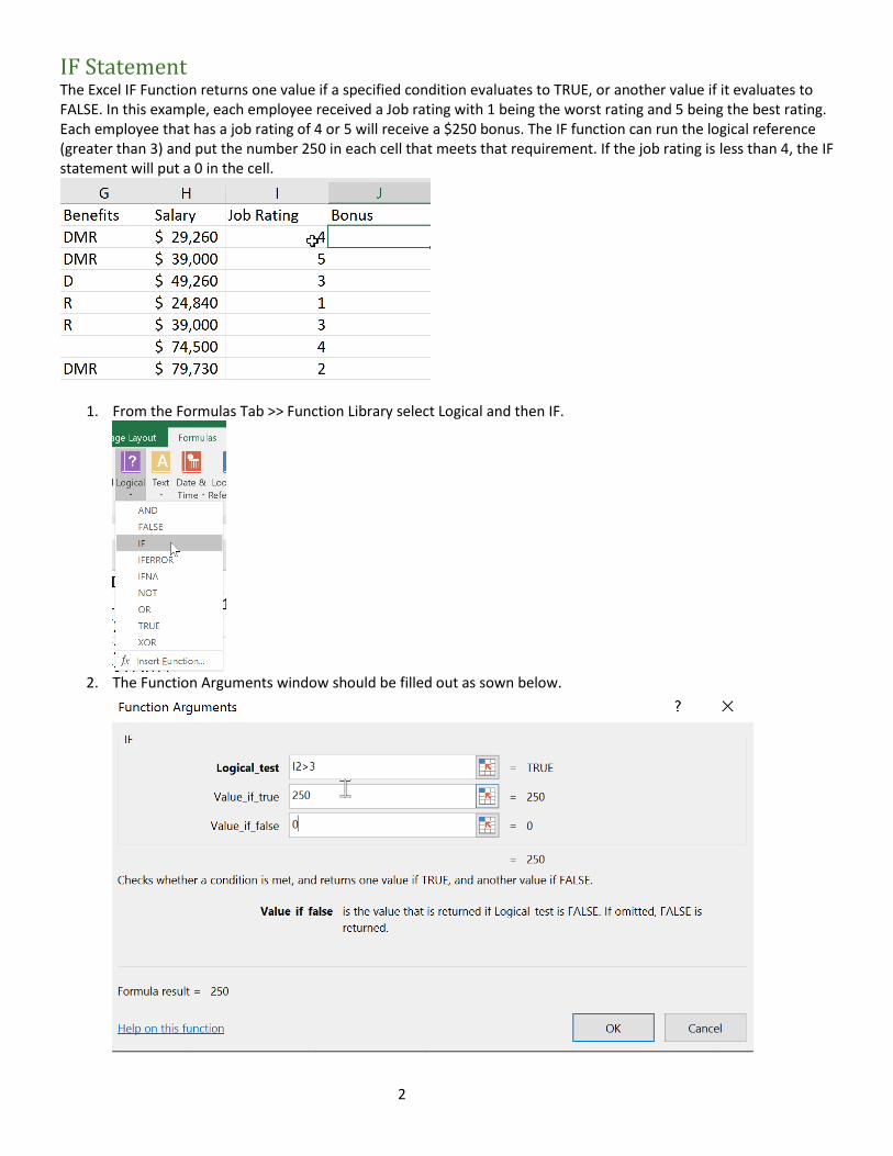
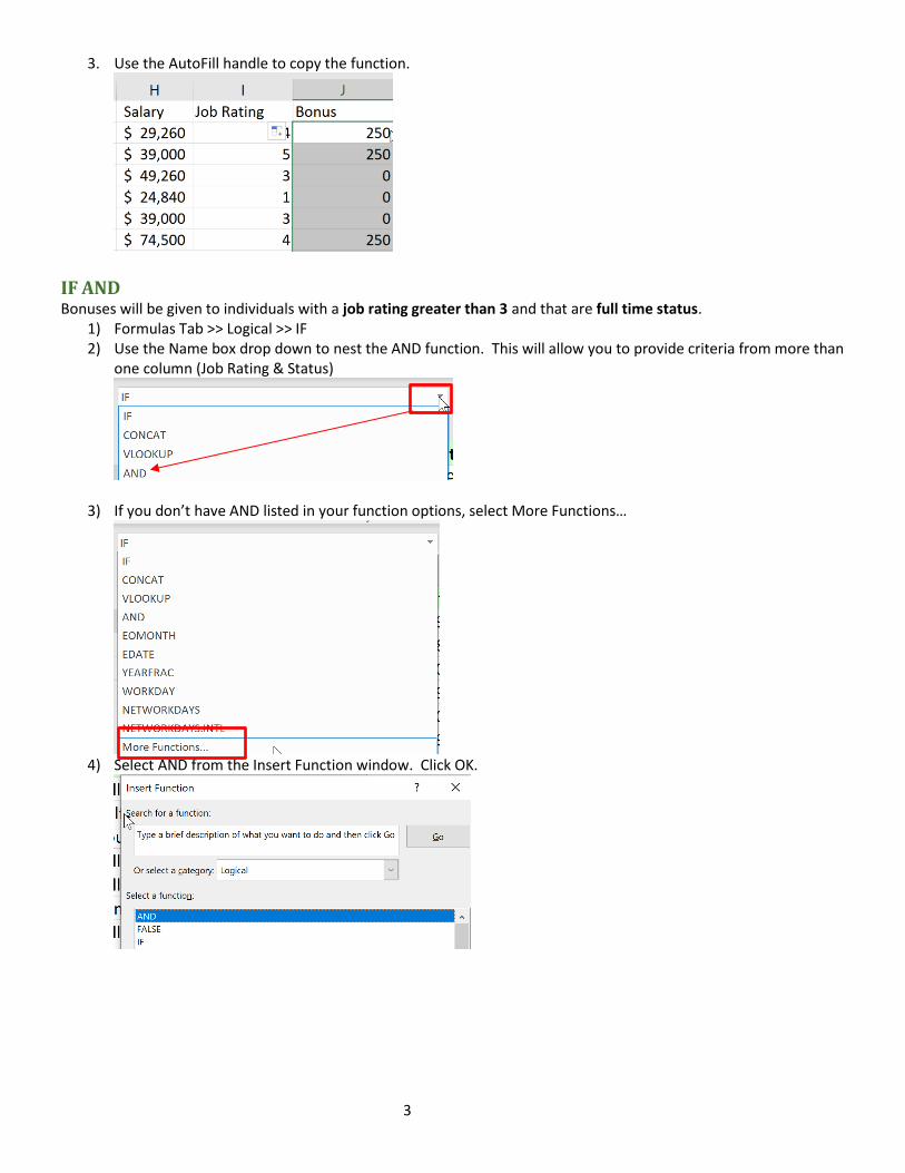
3. Use the AutoFill handle to copy the function.

IF AND Bonuses will be given to individuals with a job rating greater than 3 and that are full time status.

1) Formulas Tab >> Logical >> IF 2) Use the Name box drop down to nest the AND function. This will allow you to provide criteria from more than

one column (Job Rating & Status)

3) If you don’t have AND listed in your function options, select More Functions…

4) Select AND from the Insert Function window. Click OK.

4

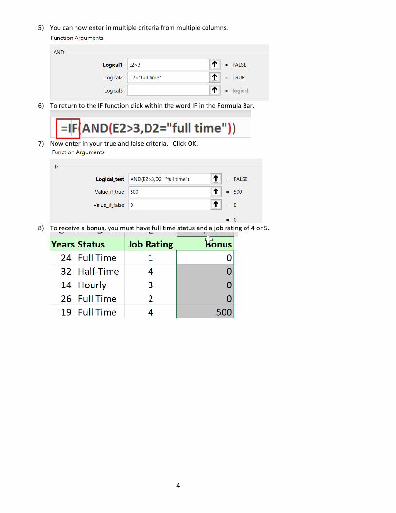
5) You can now enter in multiple criteria from multiple columns.

6) To return to the IF function click within the word IF in the Formula Bar.

7) Now enter in your true and false criteria. Click OK.

8) To receive a bonus, you must have full time status and a job rating of 4 or 5.

5

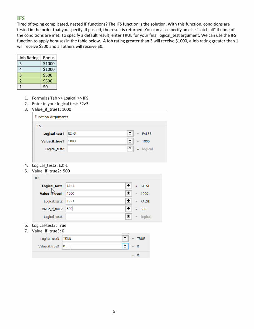
IFS Tired of typing complicated, nested IF functions? The IFS function is the solution. With this function, conditions are tested in the order that you specify. If passed, the result is returned. You can also specify an else "catch all" if none of the conditions are met. To specify a default result, enter TRUE for your final logical_test argument. We can use the IFS function to apply bonuses in the table below. A Job rating greater than 3 will receive $1000, a Job rating greater than 1 will receive $500 and all others will receive $0.

Job Rating Bonus

5 $1000

4 $1000

3 $500

2 $500

1 $0

1. Formulas Tab >> Logical >> IFS 2. Enter in your logical test: E2>3 3. Value_if_true1: 1000

4. Logical_test2: E2>1 5. Value_if_true2: 500

6. Logical-test3: True 7. Value_if_true3: 0

6

NESTED IF STATEMENT A Job rating greater than 3 will receive $1000, a Job rating greater than 1 will receive $500 and all others will receive $0.

Job Rating Bonus

5 $1000

4 $1000

3 $500

2 $500

1 $0

1. Formulas Tab >> Logical IF 2. Logical_test: E2>3

Value_if_true: 1000

3. Click in Value_if_false. Click on the IF function in the Name box.

4. Logical_test: E2>1

Value_if_true: 500 Value_if_false: 0

FORMULA WITHIN IF STATEMENT This example uses an IF statement to calculate bonuses based on excess sales targets. We will use a formula in the True part of the IF function to figure the bonus.

1. Formulas Tab >> Logical >> IF

7

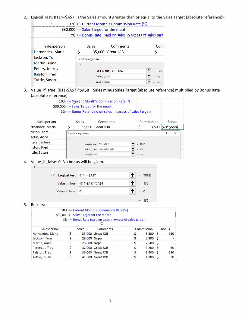
2. Logical Test: B11>=$A$7 Is the Sales amount greater than or equal to the Sales Target (absolute reference)>

3. Value_if_true: (B11-$A$7)*$A$8 Sales minus Sales Target (absolute reference) multiplied by Bonus Rate

(absolute reference)

4. Value_if_false: 0 No bonus will be given.

5. Results:

8

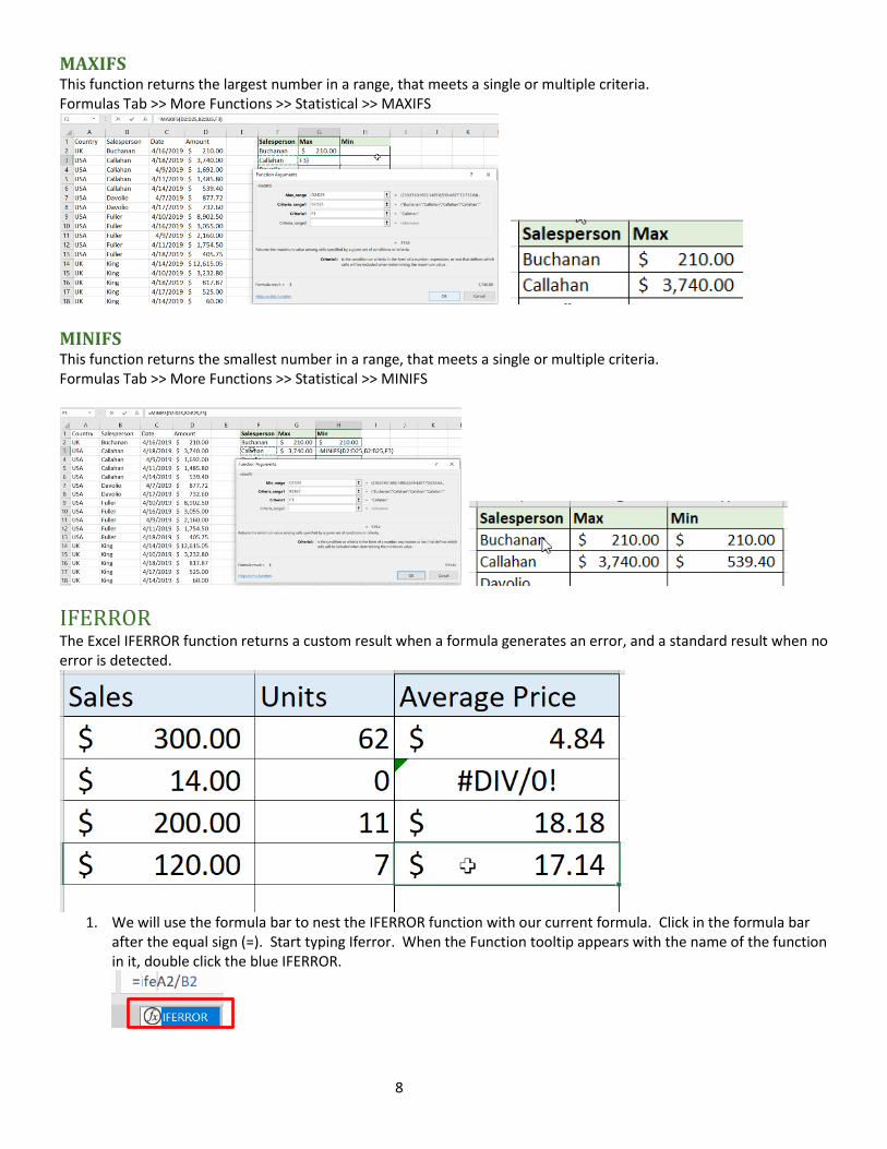
MAXIFS This function returns the largest number in a range, that meets a single or multiple criteria. Formulas Tab >> More Functions >> Statistical >> MAXIFS

MINIFS This function returns the smallest number in a range, that meets a single or multiple criteria. Formulas Tab >> More Functions >> Statistical >> MINIFS

IFERROR The Excel IFERROR function returns a custom result when a formula generates an error, and a standard result when no error is detected.

1. We will use the formula bar to nest the IFERROR function with our current formula. Click in the formula bar

after the equal sign (=). Start typing Iferror. When the Function tooltip appears with the name of the function in it, double click the blue IFERROR.

9

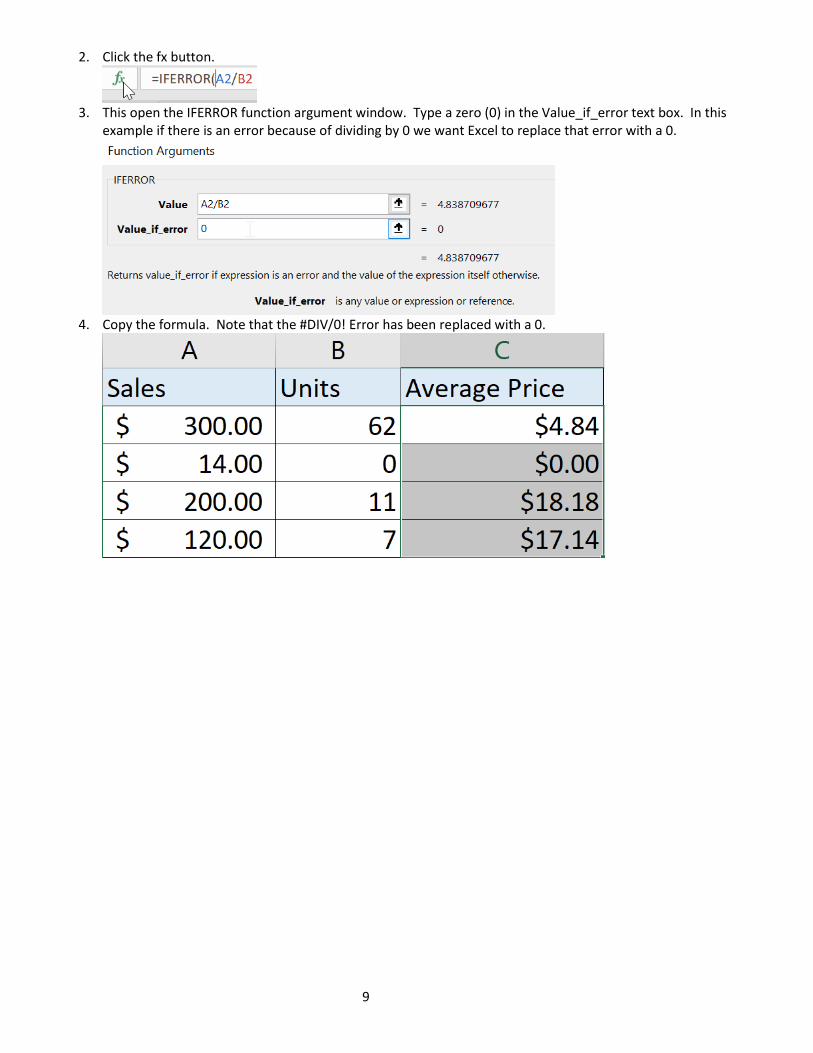
2. Click the fx button.

3. This open the IFERROR function argument window. Type a zero (0) in the Value_if_error text box. In this

example if there is an error because of dividing by 0 we want Excel to replace that error with a 0.

4. Copy the formula. Note that the #DIV/0! Error has been replaced with a 0.

10

VLOOKUP There are several Excel functions that you can use to look up and return information within a table. The most popular function for most users is VLOOKUP, which searches the first column of a range of cells and then returns a value from any cell on the same row. The inherent limitation of VLOOKUP is that whatever value you want to return must be to the right of that first search row. =VLOOKUP(lookup_value,table_array,col_index_num,[range_lookup])

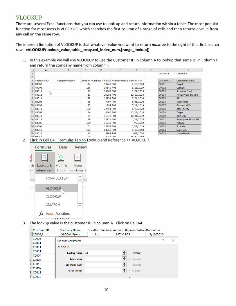
1. In this example we will use VLOOKUP to use the Customer ID in column A to lookup that same ID in Column H and return the company name from column I.

2. Click in Cell B4. Formulas Tab >> Lookup and Reference >> VLOOKUP.

3. The lookup value is the customer ID in column A. Click on Cell A4.

11

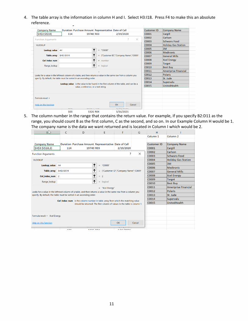
4. The table array is the information in column H and I. Select H3:I18. Press F4 to make this an absolute reference.

5. The column number in the range that contains the return value. For example, if you specify B2:D11 as the

range, you should count B as the first column, C as the second, and so on. In our Example Column H would be 1. The company name is the data we want returned and is located in Column I which would be 2.

12

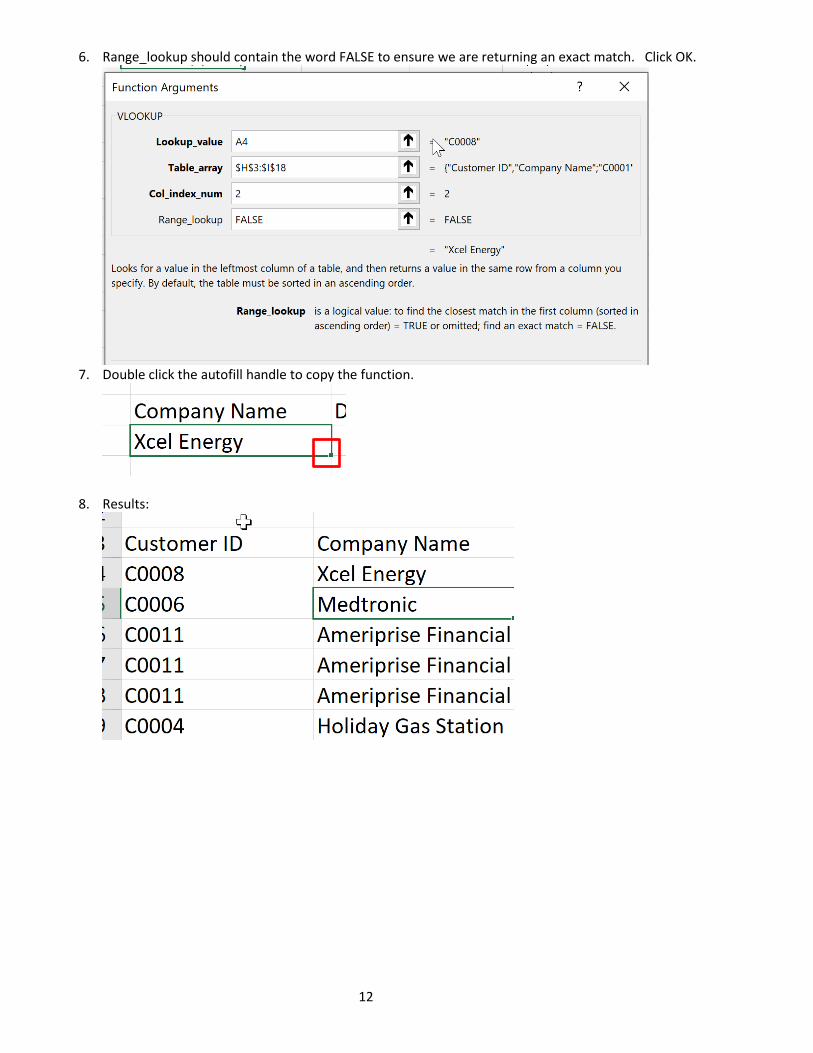
6. Range_lookup should contain the word FALSE to ensure we are returning an exact match. Click OK.

7. Double click the autofill handle to copy the function.

8. Results:

13

Creating a Table There are two ways to create a table. You can either insert a table directly in the default table style or you can convert an existing range into a table. The second approach is by far the most common:

1. On a worksheet, click anywhere in your list of information. 2. On the Home tab, within the Styles group, select Format at Table. 3. A Create Table dialog box will appear. Your selected range appears as an absolute cell reference. Your range

will already be selected and displayed in the Where is the data for your table?

4. If your selected range contains data that you want to display as table headers, select the My table has headers

check box. 5. Click the OK command button to create the table. 6. When you have an Excel table selected, you will have access to a Table Tools contextual tab with a single

Design sub-tab. Each time you create a table, Excel creates a default table name in the Properties group (e.g., Table1, Table2, etc.). The scope of the table name is for the entire workbook.

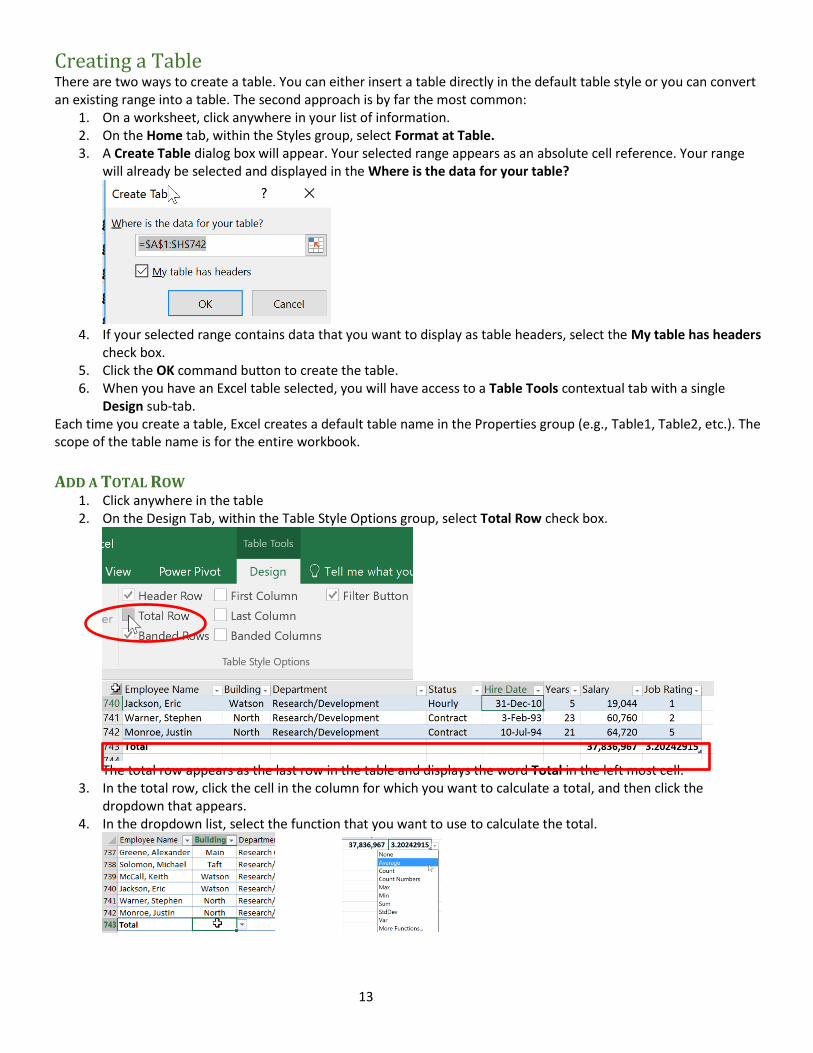
ADD A TOTAL ROW 1. Click anywhere in the table 2. On the Design Tab, within the Table Style Options group, select Total Row check box.

The total row appears as the last row in the table and displays the word Total in the left most cell.

3. In the total row, click the cell in the column for which you want to calculate a total, and then click the dropdown that appears.

4. In the dropdown list, select the function that you want to use to calculate the total.

14

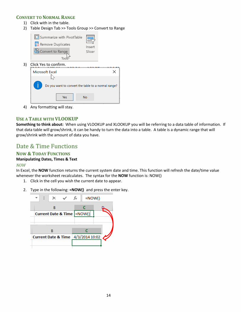
CONVERT TO NORMAL RANGE 1) Click with in the table. 2) Table Design Tab >> Tools Group >> Convert to Range

3) Click Yes to confirm.

4) Any formatting will stay.

USE A TABLE WITH VLOOKUP Something to think about: When using VLOOKUP and XLOOKUP you will be referring to a data table of information. If that data table will grow/shrink, it can be handy to turn the data into a table. A table is a dynamic range that will grow/shrink with the amount of data you have.

Date & Time Functions NOW & TODAY FUNCTIONS Manipulating Dates, Times & Text

NOW In Excel, the NOW function returns the current system date and time. This function will refresh the date/time value whenever the worksheet recalculates. The syntax for the NOW function is: NOW()

1. Click in the cell you wish the current date to appear.

2. Type in the following: =NOW() and press the enter key.

15

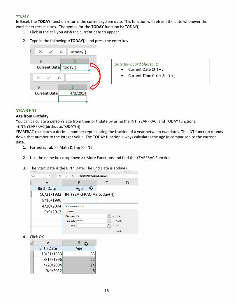
TODAY In Excel, the TODAY function returns the current system date. This function will refresh the date whenever the worksheet recalculates. The syntax for the TODAY function is: TODAY()

1. Click in the cell you wish the current date to appear.

2. Type in the following: =TODAY() and press the enter key.

YEARFAC Age from Birthday You can calculate a person’s age from their birthdate by using the INT, YEARFRAC, and TODAY functions. =(INT(YEARFRAC(birthdate,TODAY())) YEARFRAC calculates a decimal number representing the fraction of a year between two dates. The INT function rounds down that number to the integer value. The TODAY function always calculates the age in comparison to the current date.

1. Formulas Tab >> Math & Trig >> INT

2. Use the name box dropdown >> More Functions and find the YEARFRAC Function.

3. The Start Date is the Birth Date. The End Date is Today().

4. Click OK.

Date Keyboard Shortcuts • Current Date Ctrl + ;

• Current Time Ctrl + Shift + ;

16

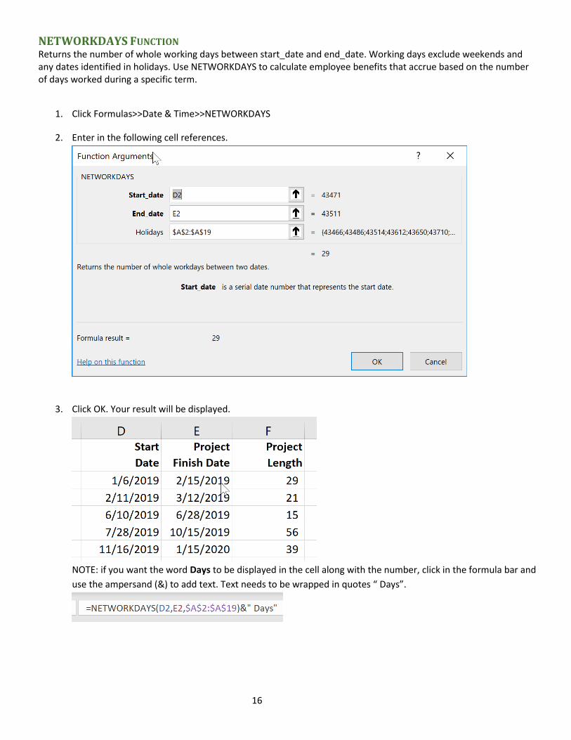
NETWORKDAYS FUNCTION Returns the number of whole working days between start_date and end_date. Working days exclude weekends and any dates identified in holidays. Use NETWORKDAYS to calculate employee benefits that accrue based on the number of days worked during a specific term.

1. Click Formulas>>Date & Time>>NETWORKDAYS

2. Enter in the following cell references.

3. Click OK. Your result will be displayed.

NOTE: if you want the word Days to be displayed in the cell along with the number, click in the formula bar and

use the ampersand (&) to add text. Text needs to be wrapped in quotes “ Days”.

17

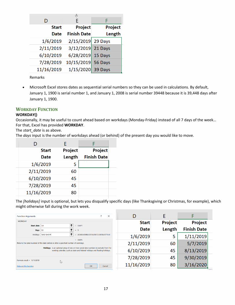
Remarks

• Microsoft Excel stores dates as sequential serial numbers so they can be used in calculations. By default,

January 1, 1900 is serial number 1, and January 1, 2008 is serial number 39448 because it is 39,448 days after

January 1, 1900.

WORKDAY FUNCTION WORKDAY() Occasionally, it may be useful to count ahead based on workdays (Monday-Friday) instead of all 7 days of the week… For that, Excel has provided WORKDAY. The start_date is as above. The days input is the number of workdays ahead (or behind) of the present day you would like to move.

The [holidays] input is optional, but lets you disqualify specific days (like Thanksgiving or Christmas, for example), which might otherwise fall during the work week.

18

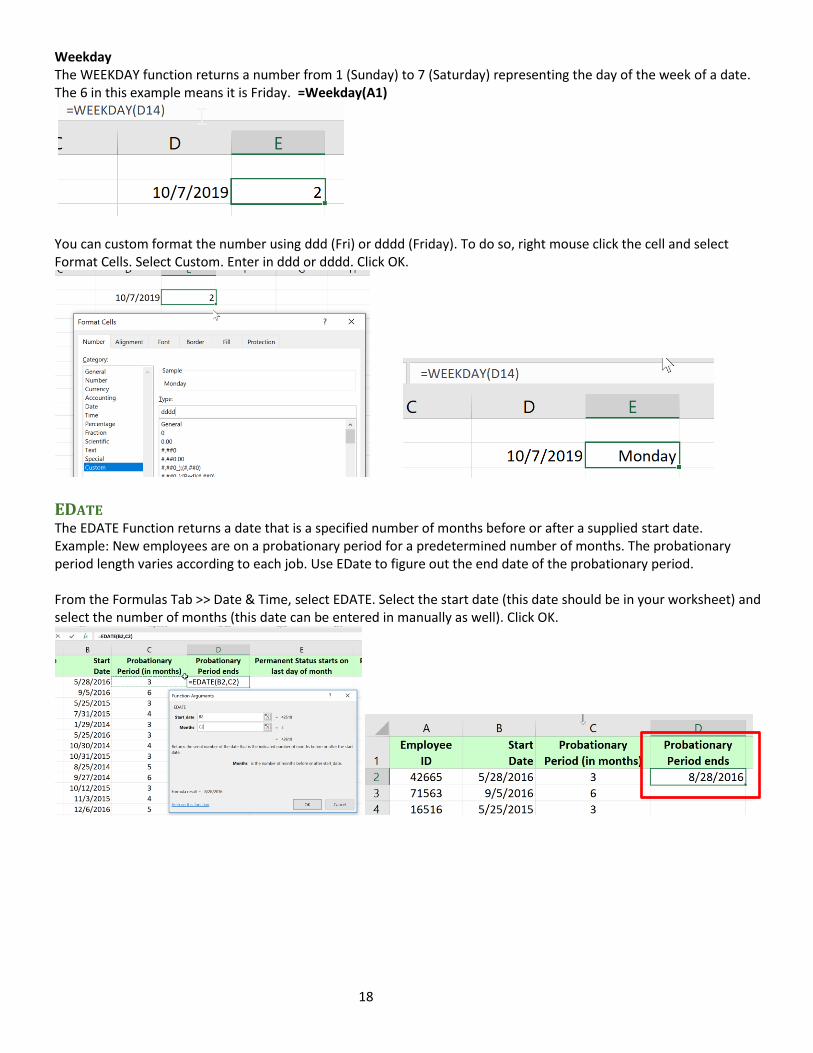
Weekday The WEEKDAY function returns a number from 1 (Sunday) to 7 (Saturday) representing the day of the week of a date. The 6 in this example means it is Friday. =Weekday(A1)

You can custom format the number using ddd (Fri) or dddd (Friday). To do so, right mouse click the cell and select Format Cells. Select Custom. Enter in ddd or dddd. Click OK.

EDATE The EDATE Function returns a date that is a specified number of months before or after a supplied start date. Example: New employees are on a probationary period for a predetermined number of months. The probationary period length varies according to each job. Use EDate to figure out the end date of the probationary period. From the Formulas Tab >> Date & Time, select EDATE. Select the start date (this date should be in your worksheet) and select the number of months (this date can be entered in manually as well). Click OK.

19

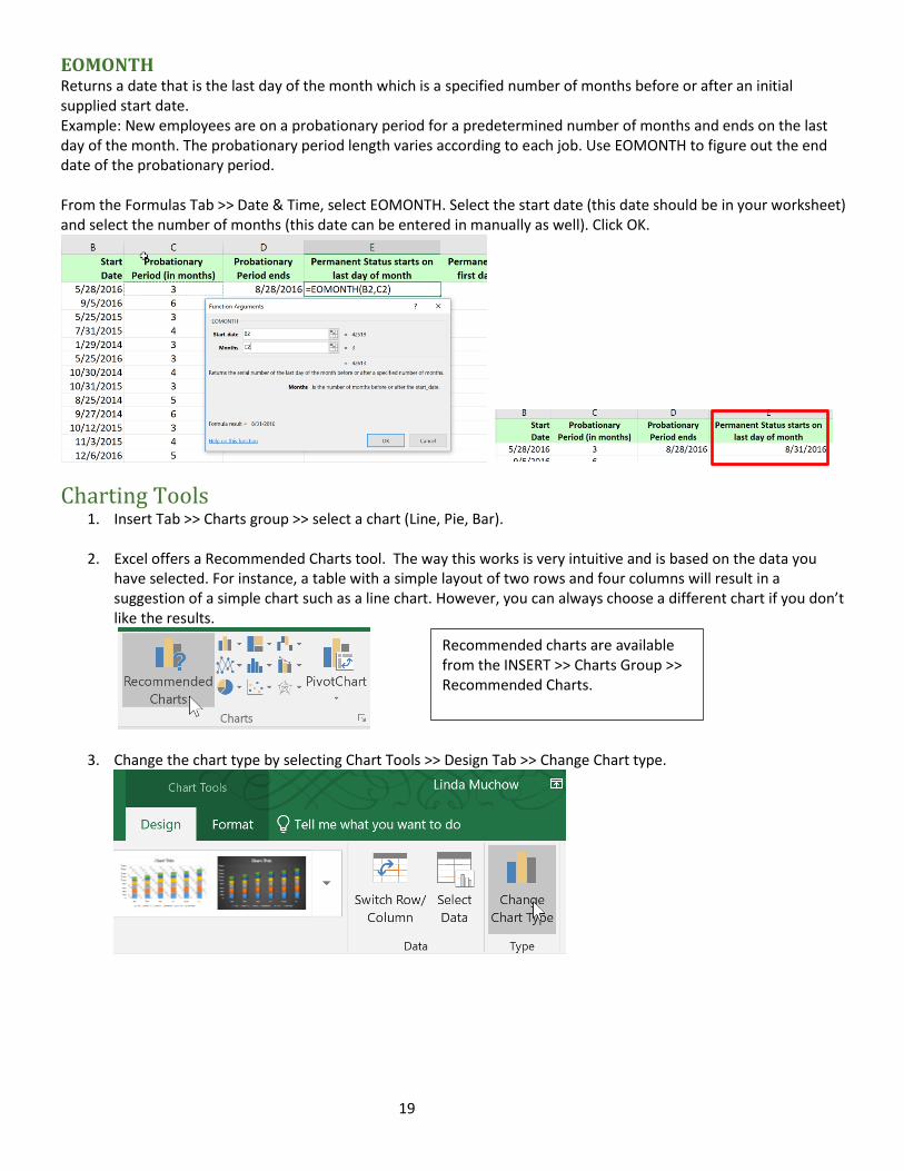
EOMONTH Returns a date that is the last day of the month which is a specified number of months before or after an initial supplied start date. Example: New employees are on a probationary period for a predetermined number of months and ends on the last day of the month. The probationary period length varies according to each job. Use EOMONTH to figure out the end date of the probationary period. From the Formulas Tab >> Date & Time, select EOMONTH. Select the start date (this date should be in your worksheet) and select the number of months (this date can be entered in manually as well). Click OK.

Charting Tools 1. Insert Tab >> Charts group >> select a chart (Line, Pie, Bar).

2. Excel offers a Recommended Charts tool. The way this works is very intuitive and is based on the data you

have selected. For instance, a table with a simple layout of two rows and four columns will result in a suggestion of a simple chart such as a line chart. However, you can always choose a different chart if you don’t like the results.

3. Change the chart type by selecting Chart Tools >> Design Tab >> Change Chart type.

Recommended charts are available from the INSERT >> Charts Group >> Recommended Charts.

20

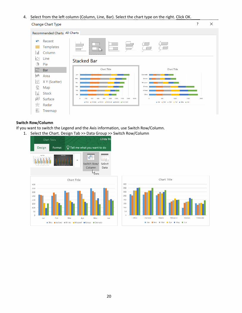
4. Select from the left column (Column, Line, Bar). Select the chart type on the right. Click OK.

Switch Row/Column If you want to switch the Legend and the Axis information, use Switch Row/Column.

1. Select the Chart. Design Tab >> Data Group >> Switch Row/Column

21

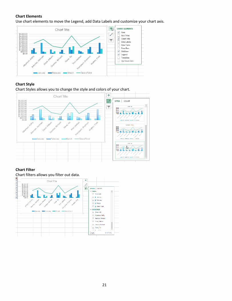
Chart Elements Use chart elements to move the Legend, add Data Labels and customize your chart axis.

Chart Style Chart Styles allows you to change the style and colors of your chart.

Chart Filter Chart filters allows you filter out data.

22

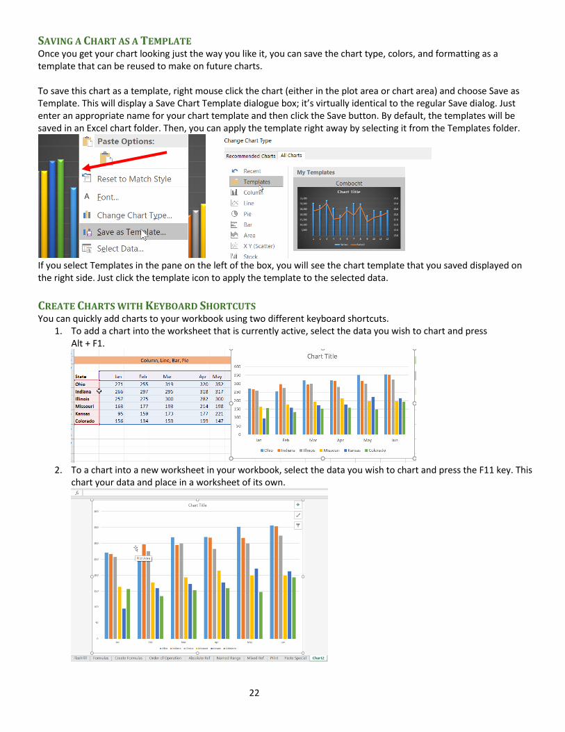
SAVING A CHART AS A TEMPLATE Once you get your chart looking just the way you like it, you can save the chart type, colors, and formatting as a template that can be reused to make on future charts. To save this chart as a template, right mouse click the chart (either in the plot area or chart area) and choose Save as Template. This will display a Save Chart Template dialogue box; it’s virtually identical to the regular Save dialog. Just enter an appropriate name for your chart template and then click the Save button. By default, the templates will be saved in an Excel chart folder. Then, you can apply the template right away by selecting it from the Templates folder.

If you select Templates in the pane on the left of the box, you will see the chart template that you saved displayed on the right side. Just click the template icon to apply the template to the selected data.

CREATE CHARTS WITH KEYBOARD SHORTCUTS You can quickly add charts to your workbook using two different keyboard shortcuts.

1. To add a chart into the worksheet that is currently active, select the data you wish to chart and press Alt + F1.

2. To a chart into a new worksheet in your workbook, select the data you wish to chart and press the F11 key. This

chart your data and place in a worksheet of its own.

23

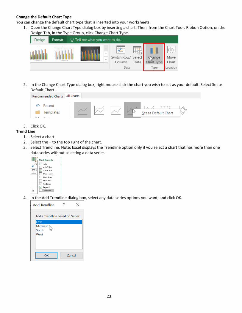
Change the Default Chart Type You can change the default chart type that is inserted into your worksheets.

1. Open the Change Chart Type dialog box by inserting a chart. Then, from the Chart Tools Ribbon Option, on the Design Tab, in the Type Group, click Change Chart Type.

2. In the Change Chart Type dialog box, right mouse click the chart you wish to set as your default. Select Set as

Default Chart.

3. Click OK. Trend Line

1. Select a chart. 2. Select the + to the top right of the chart. 3. Select Trendline. Note: Excel displays the Trendline option only if you select a chart that has more than one

data series without selecting a data series.

4. In the Add Trendline dialog box, select any data series options you want, and click OK.

24

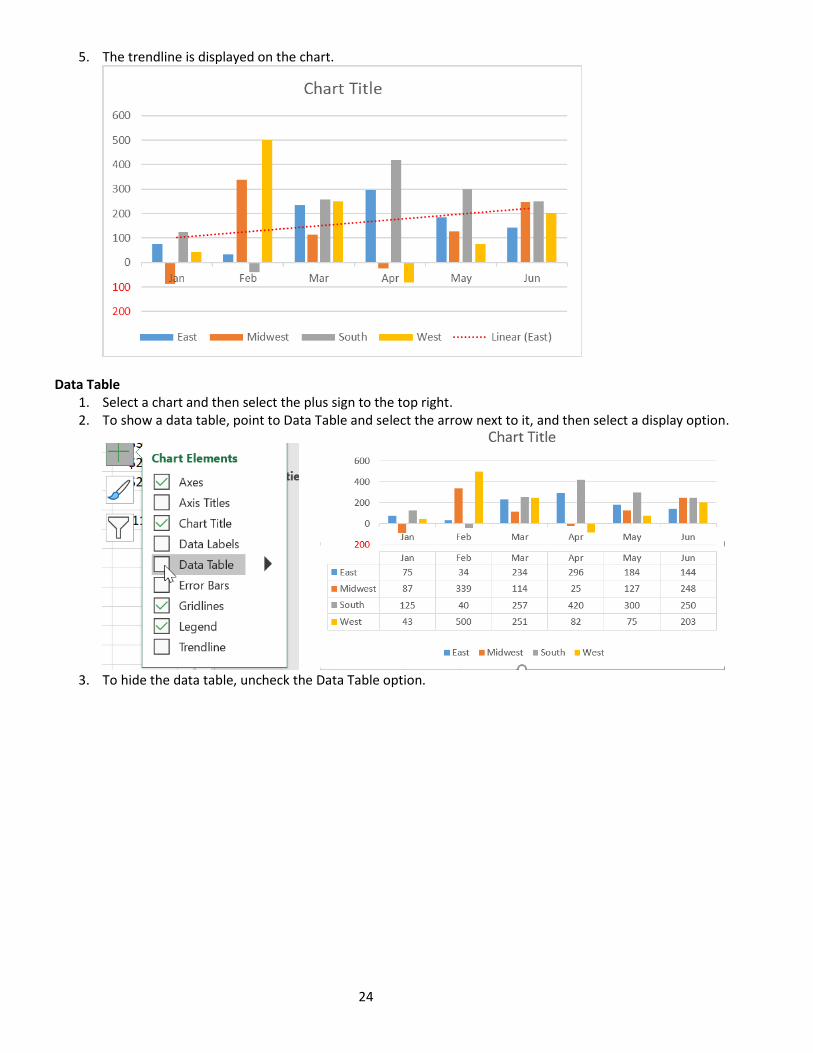
5. The trendline is displayed on the chart.

Data Table

1. Select a chart and then select the plus sign to the top right. 2. To show a data table, point to Data Table and select the arrow next to it, and then select a display option.

3. To hide the data table, uncheck the Data Table option.

25

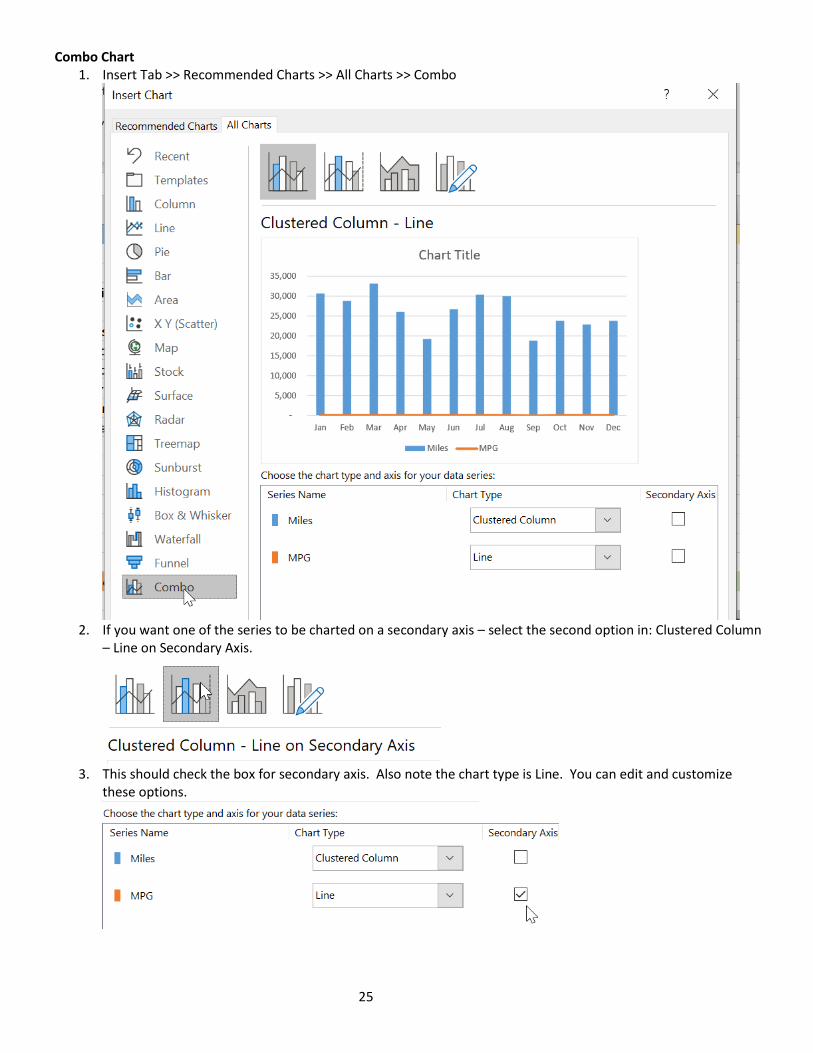
Combo Chart 1. Insert Tab >> Recommended Charts >> All Charts >> Combo

2. If you want one of the series to be charted on a secondary axis – select the second option in: Clustered Column

– Line on Secondary Axis.

3. This should check the box for secondary axis. Also note the chart type is Line. You can edit and customize

these options.

26

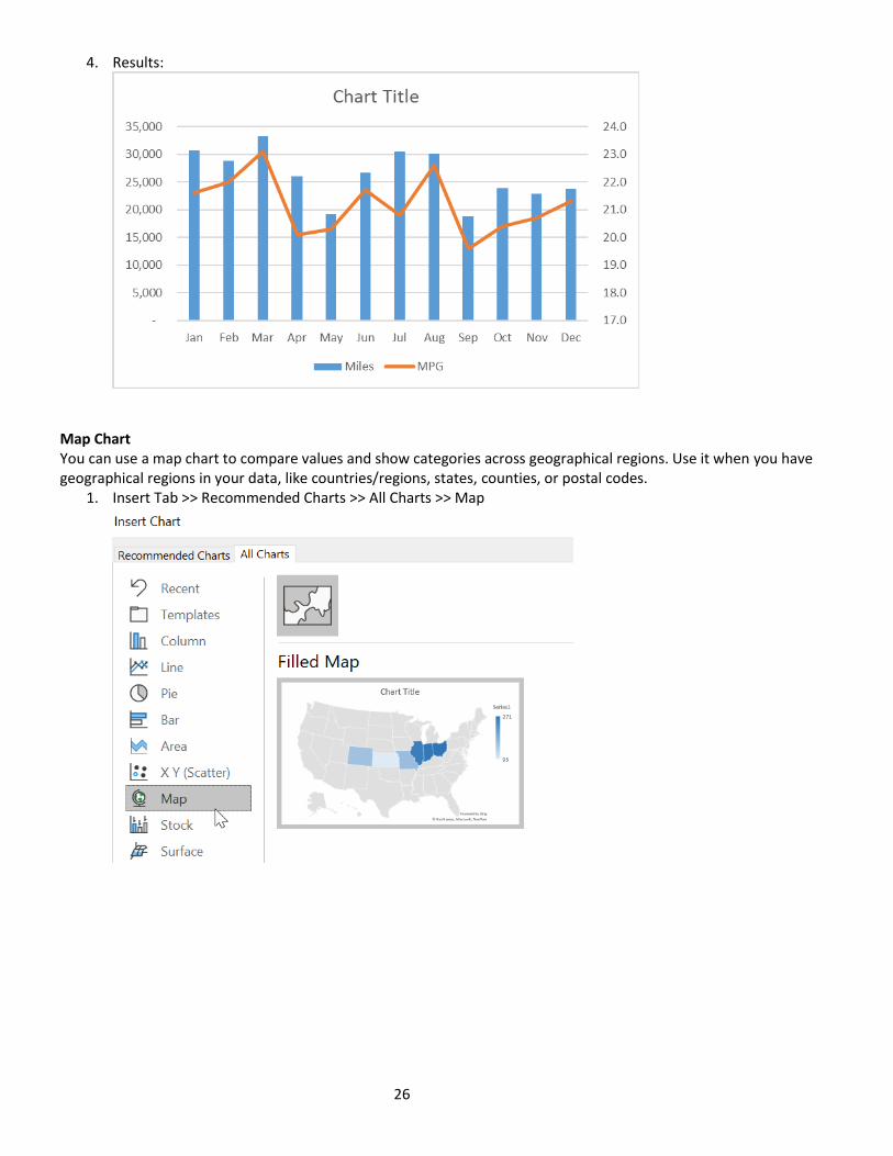
4. Results:

Map Chart You can use a map chart to compare values and show categories across geographical regions. Use it when you have geographical regions in your data, like countries/regions, states, counties, or postal codes.

1. Insert Tab >> Recommended Charts >> All Charts >> Map

27

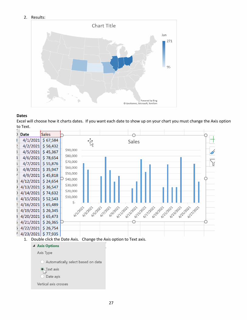
2. Results:

Dates Excel will choose how it charts dates. If you want each date to show up on your chart you must change the Axis option to Text.

1. Double click the Date Axis. Change the Axis option to Text axis.

28

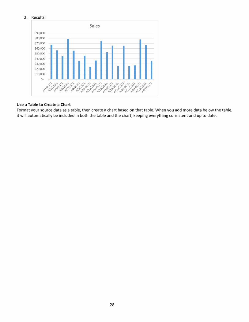
2. Results:

Use a Table to Create a Chart Format your source data as a table, then create a chart based on that table. When you add more data below the table, it will automatically be included in both the table and the chart, keeping everything consistent and up to date.

29

Custom Formats - Excel Number formatting in Excel is used to change the way a value appears in a cell or range of cells. Number formatting does not actually alter the value, it only changes the way we see it. When one formats a cell one typically uses the Format Cells dialog box. You can right mouse click and select Format Cells, use the keyboard shortcut Ctrl + 1 or from the Home tab, within the Cells group, select Format >> Format Cells >> Custom

TEXT CHARACTERS & SPACING To display both text and numbers in a cell, enclose the text characters in double quotation marks (" ") or precede a single character with a backslash (\). Include the characters in the appropriate section of the format codes. For example, type the format $0.00" Surplus";$-0.00" Shortage" to display a positive amount as "$125.74 Surplus" and a negative amount as "$-125.74 Shortage." The following characters are displayed without the use of quotation marks:

$ Dollar sign

- Negative sign

+ Plus sign

/ Solidus (slash) ( Left parenthesis

) Right parenthesis

: Colon

! Exclamation mark ^ Circumflex accent (caret)

& Ampersand

' Apostrophe

~ Tilde { Left curly bracket

} Right curly bracket

< Less-than sign

> Greater-than sign = Equals sign

Space character

Including a section for text entry If included, a text section is always the last section in the number format. Include an at sign (@) in the section where you want to display any text entered in the cell. If the @ character is omitted from the text section, text you enter will not be displayed. If you want to always display specific text characters with the entered text, enclose the additional text in double quotation marks (" "). For example, "gross receipts for "@ If the format does not include a text section, text you enter is not affected by the format.

30

Adding spaces To create a space the width of a character in a number format, include an underscore, followed by the character. For example, when you follow an underscore with a right parenthesis, such as _), positive numbers line up correctly with negative numbers that are enclosed in parentheses. Repeating characters To repeat the next character in the format to fill the column width, include an asterisk (*) in the number format. For example, type 0*- to include enough dashes after a number to fill the cell, or type *0 before any format to include leading zeros.

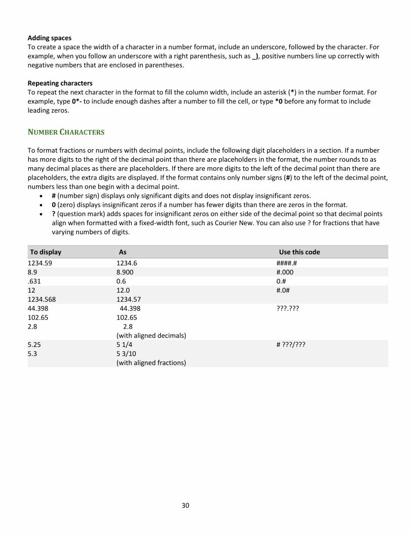
NUMBER CHARACTERS To format fractions or numbers with decimal points, include the following digit placeholders in a section. If a number has more digits to the right of the decimal point than there are placeholders in the format, the number rounds to as many decimal places as there are placeholders. If there are more digits to the left of the decimal point than there are placeholders, the extra digits are displayed. If the format contains only number signs (#) to the left of the decimal point, numbers less than one begin with a decimal point.

• # (number sign) displays only significant digits and does not display insignificant zeros. • 0 (zero) displays insignificant zeros if a number has fewer digits than there are zeros in the format. • ? (question mark) adds spaces for insignificant zeros on either side of the decimal point so that decimal points

align when formatted with a fixed-width font, such as Courier New. You can also use ? for fractions that have varying numbers of digits.

To display As Use this code

1234.59 1234.6 ####.# 8.9 8.900 #.000 .631 0.6 0.# 12 1234.568

12.0 1234.57

#.0#

44.398 102.65 2.8

44.398 102.65 2.8 (with aligned decimals)

???.???

5.25 5.3

5 1/4 5 3/10 (with aligned fractions)

# ???/???

31

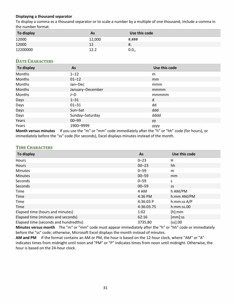
Displaying a thousand separator To display a comma as a thousand separator or to scale a number by a multiple of one thousand, include a comma in the number format.

To display As Use this code

12000 12,000 #,### 12000 12 #, 12200000 12.2 0.0,,

DATE CHARACTERS

To display As Use this code

Months 1–12 m Months 01–12 mm Months Jan–Dec mmm Months January–December mmmm Months J–D mmmmm Days 1–31 d Days 01–31 dd Days Sun–Sat ddd Days Sunday–Saturday dddd Years 00–99 yy Years 1900–9999 yyyy Month versus minutes If you use the "m" or "mm" code immediately after the "h" or "hh" code (for hours), or immediately before the "ss" code (for seconds), Excel displays minutes instead of the month.

TIME CHARACTERS

To display As Use this code

Hours 0–23 H Hours 00–23 hh Minutes 0–59 m Minutes 00–59 mm Seconds 0–59 s Seconds 00–59 ss Time 4 AM h AM/PM Time 4:36 PM h:mm AM/PM Time 4:36:03 P h:mm:ss A/P Time 4:36:03.75 h:mm:ss.00 Elapsed time (hours and minutes) 1:02 [h]:mm Elapsed time (minutes and seconds) 62:16 [mm]:ss Elapsed time (seconds and hundredths) 3735.80 [ss].00 Minutes versus month The "m" or "mm" code must appear immediately after the "h" or "hh" code or immediately before the "ss" code; otherwise, Microsoft Excel displays the month instead of minutes. AM and PM If the format contains an AM or PM, the hour is based on the 12-hour clock, where "AM" or "A" indicates times from midnight until noon and "PM" or "P" indicates times from noon until midnight. Otherwise, the hour is based on the 24-hour clock.

Excel: Tables and PivotTables Linda Muchow Alexandria Technical & Community College

[email protected]

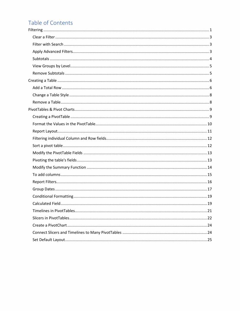
Table of Contents Filtering ......................................................................................................................................................... 1

Clear a Filter .............................................................................................................................................. 3

Filter with Search ...................................................................................................................................... 3

Apply Advanced Filters.............................................................................................................................. 3

Subtotals ................................................................................................................................................... 4

View Groups by Level ................................................................................................................................ 5

Remove Subtotals ..................................................................................................................................... 5

Creating a Table ............................................................................................................................................ 6

Add a Total Row ........................................................................................................................................ 6

Change a Table Style ................................................................................................................................. 8

Remove a Table ......................................................................................................................................... 8

PivotTables & Pivot Charts ............................................................................................................................ 9

Creating a PivotTable ................................................................................................................................ 9

Format the Values in the PivotTable ....................................................................................................... 10

Report Layout .......................................................................................................................................... 11

Filtering individual Column and Row fields............................................................................................. 12

Sort a pivot table ..................................................................................................................................... 12

Modify the PivotTable Fields .................................................................................................................. 13

Pivoting the table's fields ........................................................................................................................ 13

Modify the Summary Function ............................................................................................................... 14

To add columns ....................................................................................................................................... 15

Report Filters........................................................................................................................................... 16

Group Dates ............................................................................................................................................ 17

Conditional Formatting ........................................................................................................................... 19

Calculated Field ....................................................................................................................................... 19

Timelines in PivotTables.......................................................................................................................... 21

Slicers in PivotTables ............................................................................................................................... 22

Create a PivotChart ................................................................................................................................. 24

Connect Slicers and Timelines to Many PivotTables .............................................................................. 24

Set Default Layout ................................................................................................................................... 25

1

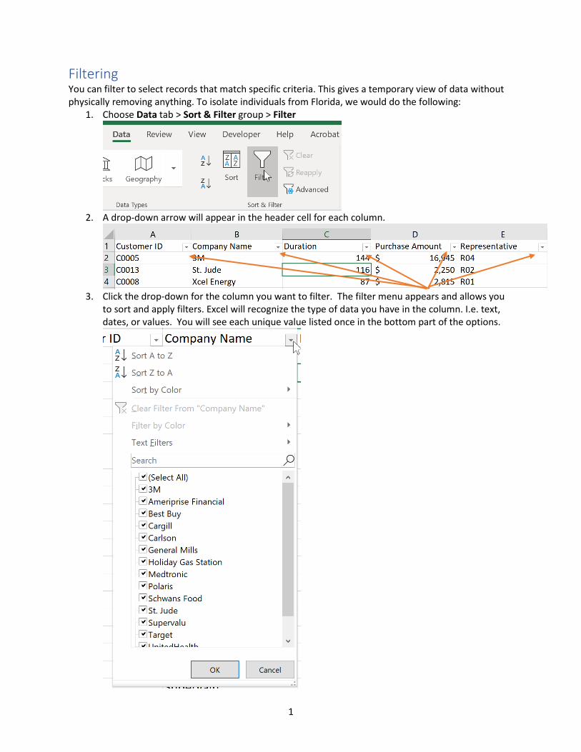
Filtering You can filter to select records that match specific criteria. This gives a temporary view of data without physically removing anything. To isolate individuals from Florida, we would do the following:

1. Choose Data tab > Sort & Filter group > Filter

2. A drop-down arrow will appear in the header cell for each column.

3. Click the drop-down for the column you want to filter. The filter menu appears and allows youto sort and apply filters. Excel will recognize the type of data you have in the column. I.e. text,dates, or values. You will see each unique value listed once in the bottom part of the options.

2

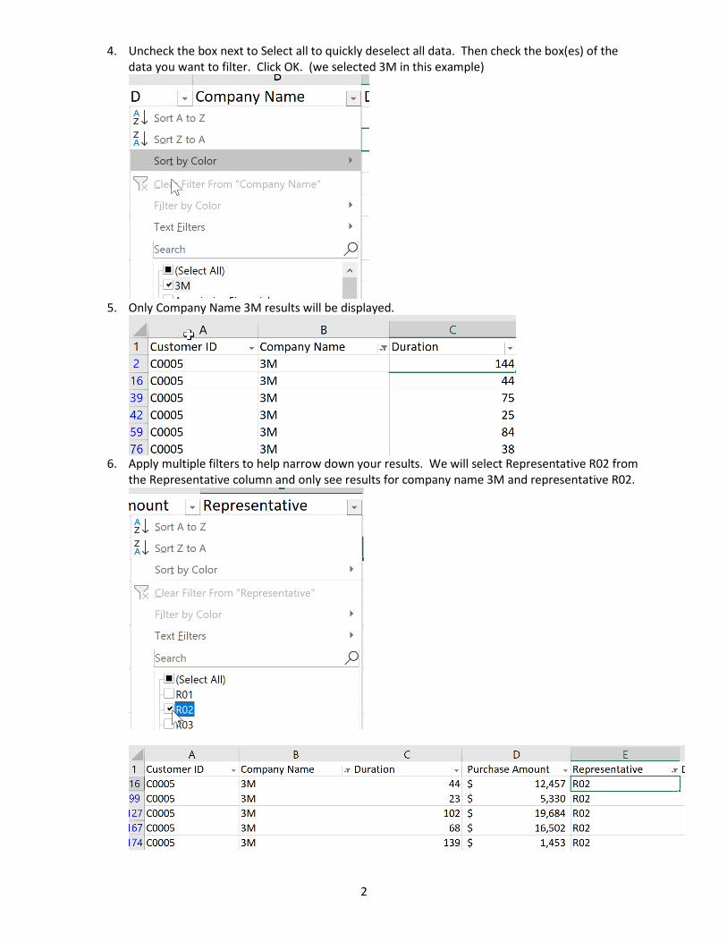
4. Uncheck the box next to Select all to quickly deselect all data. Then check the box(es) of thedata you want to filter. Click OK. (we selected 3M in this example)

5. Only Company Name 3M results will be displayed.

6. Apply multiple filters to help narrow down your results. We will select Representative R02 fromthe Representative column and only see results for company name 3M and representative R02.

3

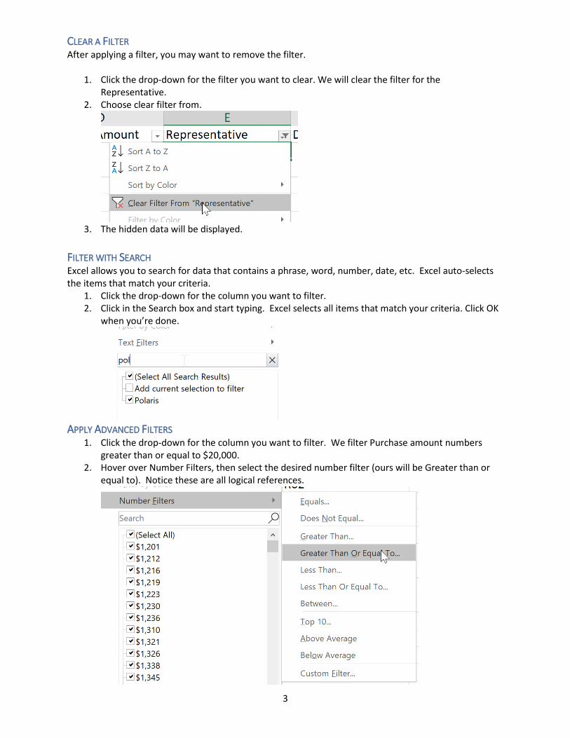
CLEAR A FILTER After applying a filter, you may want to remove the filter.

1. Click the drop-down for the filter you want to clear. We will clear the filter for theRepresentative.

2. Choose clear filter from.

3. The hidden data will be displayed.

FILTER WITH SEARCH Excel allows you to search for data that contains a phrase, word, number, date, etc. Excel auto-selects the items that match your criteria.

1. Click the drop-down for the column you want to filter.2. Click in the Search box and start typing. Excel selects all items that match your criteria. Click OK

when you’re done.

APPLY ADVANCED FILTERS 1. Click the drop-down for the column you want to filter. We filter Purchase amount numbers

greater than or equal to $20,000.2. Hover over Number Filters, then select the desired number filter (ours will be Greater than or

equal to). Notice these are all logical references.

4

3. Type in the desired number(s) to the right of each filter. Click OK.

4. Only numbers that are 20,000 and greater are displayed.

SUBTOTALS 1. Sort the list on the field for which you want subtotals inserted. Data Tab >> Sort & Filter >> AZ

2. From the Data tab, in the Outline group, select Subtotal.3. Select the field for which the subtotals are to be calculated in the At Each Change in dropdown.4. Specify the types of totals you want to insert in the Use Function dropdown.5. Select the check boxes for the field(s) you want to total in the Add Subtotal To list box.6. Click OK.

5

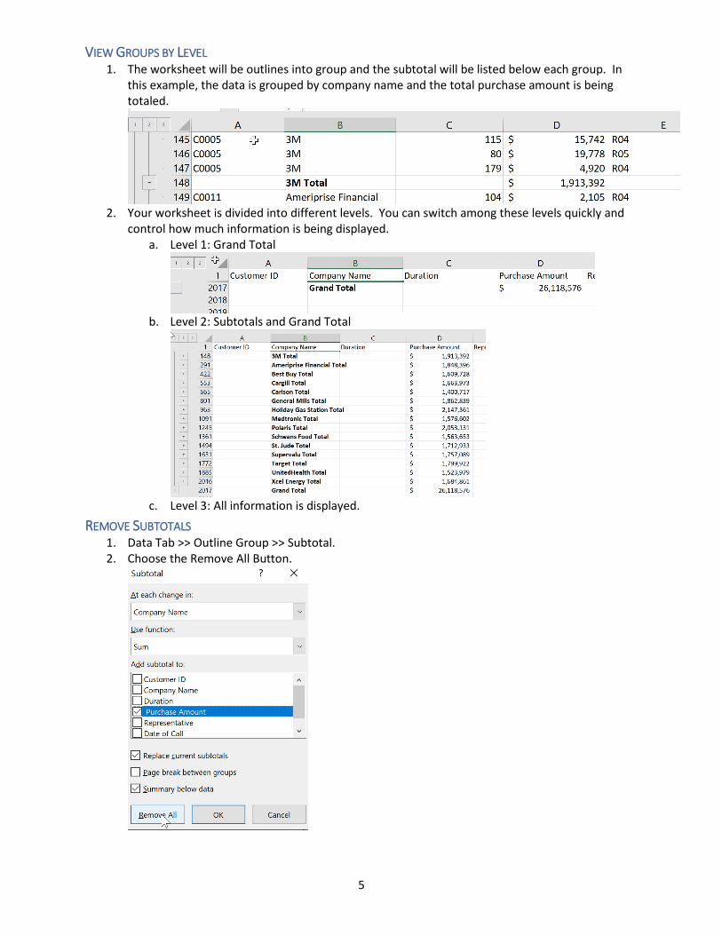
VIEW GROUPS BY LEVEL 1. The worksheet will be outlines into group and the subtotal will be listed below each group. In

this example, the data is grouped by company name and the total purchase amount is beingtotaled.

2. Your worksheet is divided into different levels. You can switch among these levels quickly andcontrol how much information is being displayed.

a. Level 1: Grand Total

b. Level 2: Subtotals and Grand Total

c. Level 3: All information is displayed.REMOVE SUBTOTALS

1. Data Tab >> Outline Group >> Subtotal.2. Choose the Remove All Button.

6

Creating a Table There are two ways to create a table. You can either insert a table directly in the default table style or you can convert an existing range into a table. The second approach is by far the most common:

1. Insert Tab >> Table.

2. A Create Table dialog box will appear. Your selected range appears as an absolute cell reference.Your range will already be selected and displayed in the Where is the data for your table?

3. If your selected range contains data that you want to display as table headers, select the Mytable has headers check box.

4. Click the OK command button to create the table.5. When you have an Excel table selected, you will have access to a Table Tools contextual tab

with a single Design sub-tab.Each time you create a table, Excel creates a default table name in the Properties group (e.g., Table1, Table2, etc.). The scope of the table name is for the entire workbook.

ADD A TOTAL ROW 1. Click anywhere in the table.2. On the Design Tab, within the Table Style Options group, select Total Row check box.

7

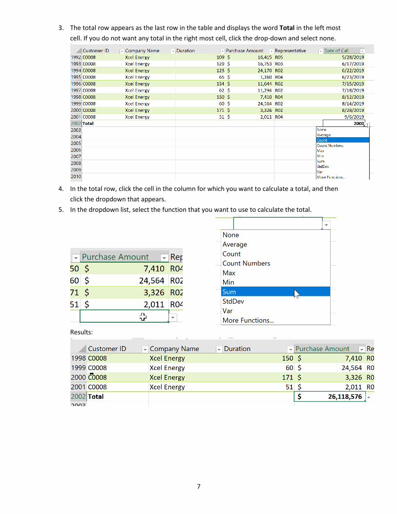
3. The total row appears as the last row in the table and displays the word Total in the left mostcell. If you do not want any total in the right most cell, click the drop-down and select none.

4. In the total row, click the cell in the column for which you want to calculate a total, and thenclick the dropdown that appears.

5. In the dropdown list, select the function that you want to use to calculate the total.

Results:

8

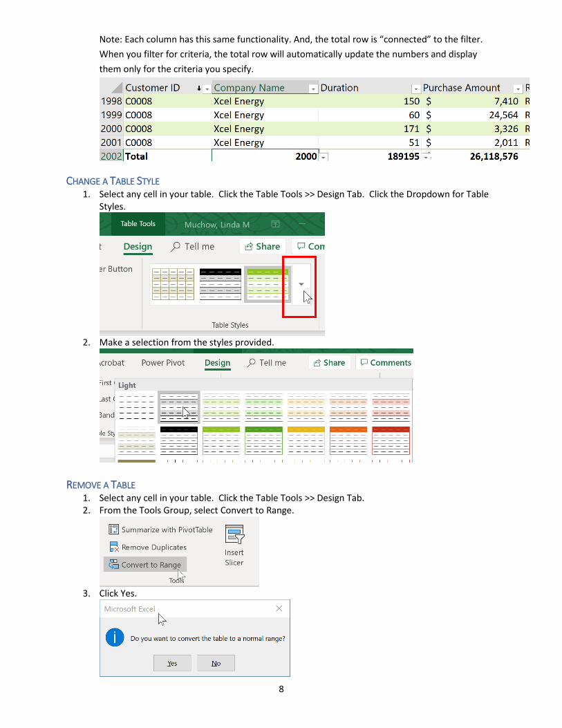
Note: Each column has this same functionality. And, the total row is “connected” to the filter. When you filter for criteria, the total row will automatically update the numbers and display them only for the criteria you specify.

CHANGE A TABLE STYLE 1. Select any cell in your table. Click the Table Tools >> Design Tab. Click the Dropdown for Table

Styles.

2. Make a selection from the styles provided.

REMOVE A TABLE 1. Select any cell in your table. Click the Table Tools >> Design Tab.2. From the Tools Group, select Convert to Range.

3. Click Yes.

9

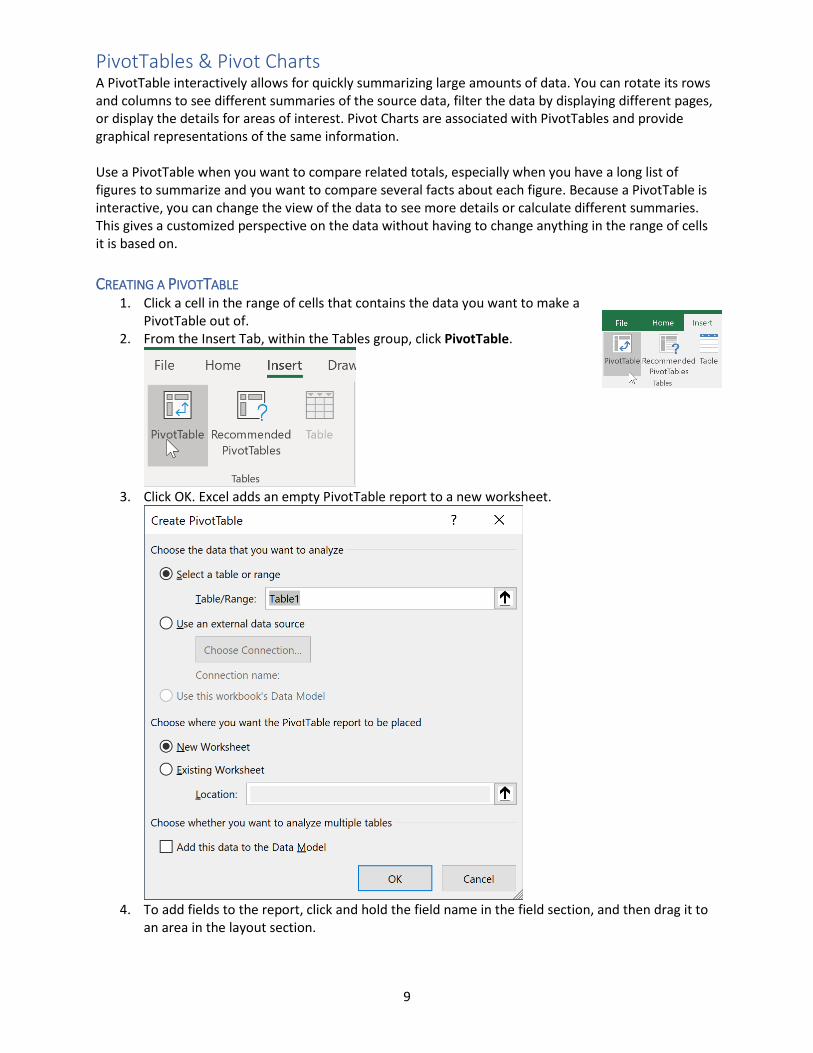
PivotTables & Pivot Charts A PivotTable interactively allows for quickly summarizing large amounts of data. You can rotate its rows and columns to see different summaries of the source data, filter the data by displaying different pages, or display the details for areas of interest. Pivot Charts are associated with PivotTables and provide graphical representations of the same information.

Use a PivotTable when you want to compare related totals, especially when you have a long list of figures to summarize and you want to compare several facts about each figure. Because a PivotTable is interactive, you can change the view of the data to see more details or calculate different summaries. This gives a customized perspective on the data without having to change anything in the range of cells it is based on.

CREATING A PIVOTTABLE 1. Click a cell in the range of cells that contains the data you want to make a

PivotTable out of.2. From the Insert Tab, within the Tables group, click PivotTable.

3. Click OK. Excel adds an empty PivotTable report to a new worksheet.

4. To add fields to the report, click and hold the field name in the field section, and then drag it toan area in the layout section.

10

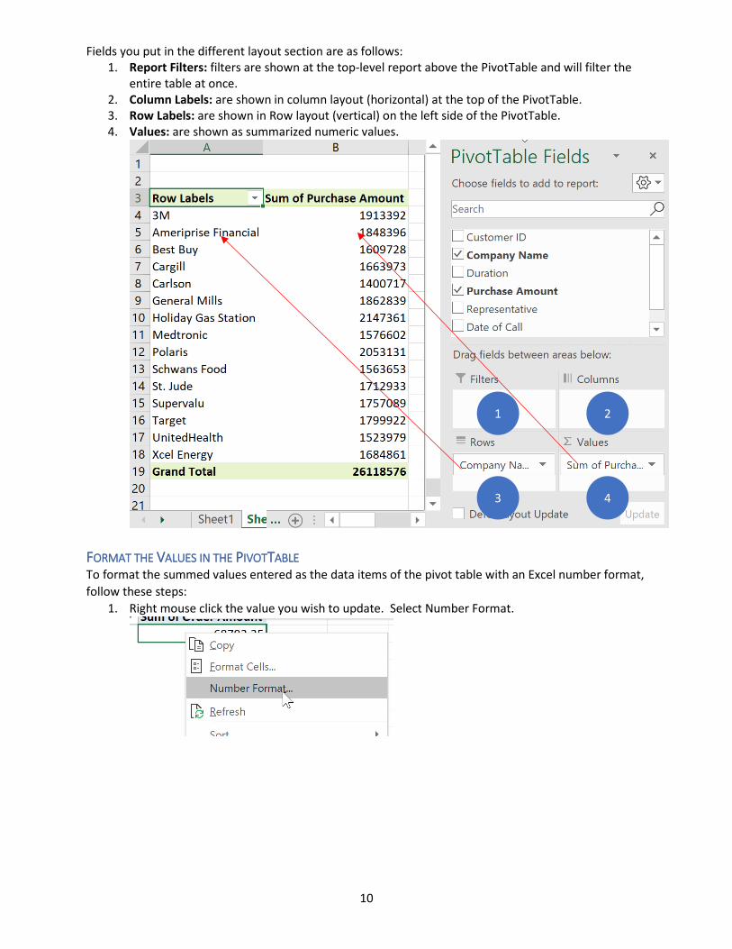
Fields you put in the different layout section are as follows: 1. Report Filters: filters are shown at the top-level report above the PivotTable and will filter the

entire table at once. 2. Column Labels: are shown in column layout (horizontal) at the top of the PivotTable. 3. Row Labels: are shown in Row layout (vertical) on the left side of the PivotTable. 4. Values: are shown as summarized numeric values.

FORMAT THE VALUES IN THE PIVOTTABLE To format the summed values entered as the data items of the pivot table with an Excel number format, follow these steps:

1. Right mouse click the value you wish to update. Select Number Format.

1 2

3 4

11

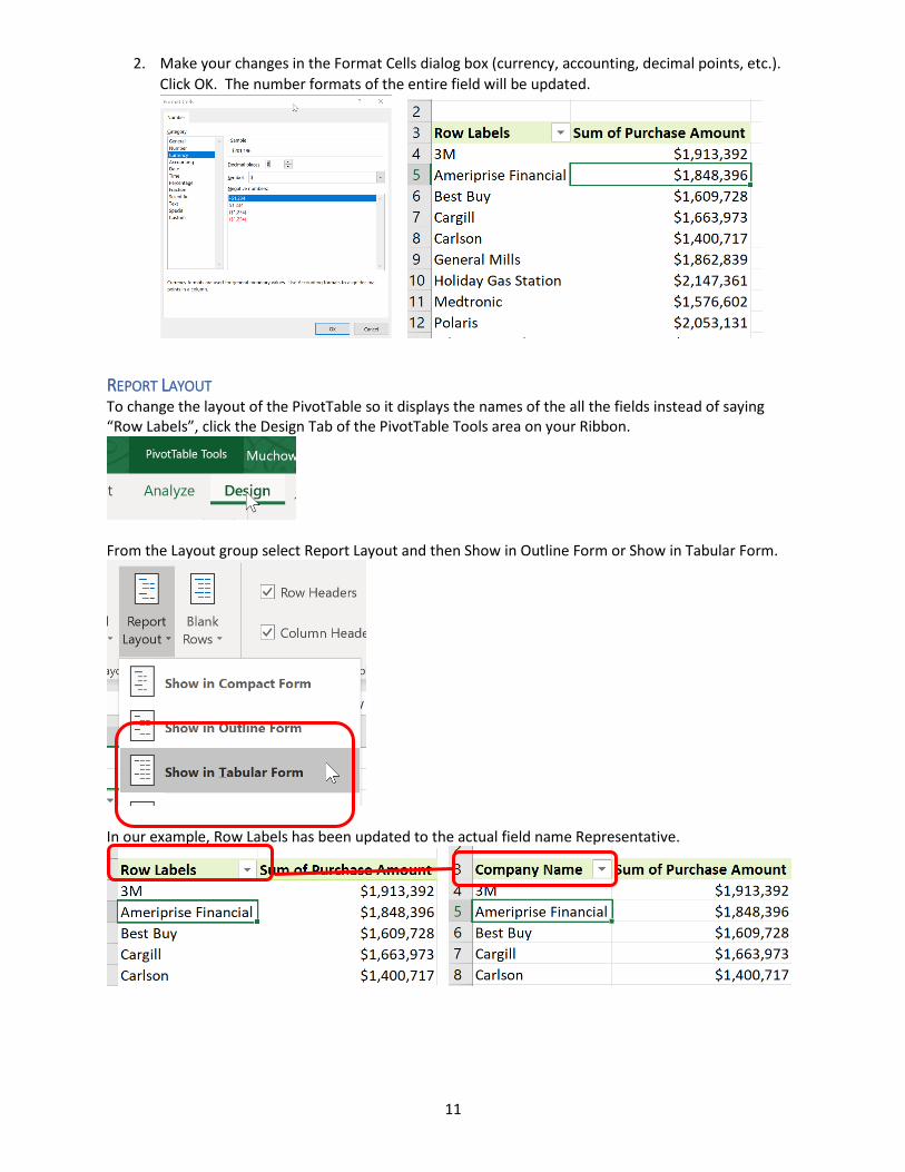
2. Make your changes in the Format Cells dialog box (currency, accounting, decimal points, etc.). Click OK. The number formats of the entire field will be updated.

REPORT LAYOUT To change the layout of the PivotTable so it displays the names of the all the fields instead of saying “Row Labels”, click the Design Tab of the PivotTable Tools area on your Ribbon.

From the Layout group select Report Layout and then Show in Outline Form or Show in Tabular Form.

In our example, Row Labels has been updated to the actual field name Representative.

12

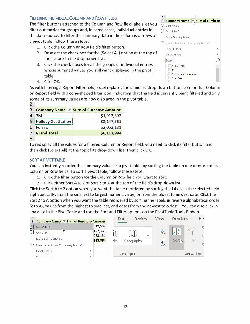
FILTERING INDIVIDUAL COLUMN AND ROW FIELDS The filter buttons attached to the Column and Row field labels let you filter out entries for groups and, in some cases, individual entries in the data source. To filter the summary data in the columns or rows of a pivot table, follow these steps:

1. Click the Column or Row field's filter button. 2. Deselect the check box for the (Select All) option at the top of

the list box in the drop-down list. 3. Click the check boxes for all the groups or individual entries

whose summed values you still want displayed in the pivot table.

4. Click OK. As with filtering a Report Filter field, Excel replaces the standard drop-down button icon for that Column or Report field with a cone-shaped filter icon, indicating that the field is currently being filtered and only some of its summary values are now displayed in the pivot table.

To redisplay all the values for a filtered Column or Report field, you need to click its filter button and then click (Select All) at the top of its drop-down list. Then click OK.

SORT A PIVOT TABLE You can instantly reorder the summary values in a pivot table by sorting the table on one or more of its Column or Row fields. To sort a pivot table, follow these steps:

1. Click the filter button for the Column or Row field you want to sort. 2. Click either Sort A to Z or Sort Z to A at the top of the field's drop-down list.

Click the Sort A to Z option when you want the table reordered by sorting the labels in the selected field alphabetically, from the smallest to largest numeric value, or from the oldest to newest date. Click the Sort Z to A option when you want the table reordered by sorting the labels in reverse alphabetical order (Z to A), values from the highest to smallest, and dates from the newest to oldest. You can also click in any data in the PivotTable and use the Sort and Filter options on the PivotTable Tools Ribbon.

13

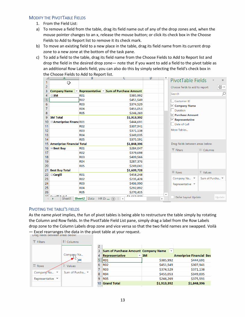
MODIFY THE PIVOTTABLE FIELDS 1. From the Field List: a) To remove a field from the table, drag its field name out of any of the drop zones and, when the

mouse pointer changes to an x, release the mouse button; or click its check box in the Choose Fields to Add to Report list to remove it its check mark.

b) To move an existing field to a new place in the table, drag its field name from its current drop zone to a new zone at the bottom of the task pane.

c) To add a field to the table, drag its field name from the Choose Fields to Add to Report list and drop the field in the desired drop zone— note that if you want to add a field to the pivot table as an additional Row Labels field, you can also do this by simply selecting the field's check box in the Choose Fields to Add to Report list.

PIVOTING THE TABLE'S FIELDS As the name pivot implies, the fun of pivot tables is being able to restructure the table simply by rotating the Column and Row fields. In the PivotTable Field List pane, simply drag a label from the Row Labels drop zone to the Column Labels drop zone and vice versa so that the two field names are swapped. Voilà — Excel rearranges the data in the pivot table at your request.

14

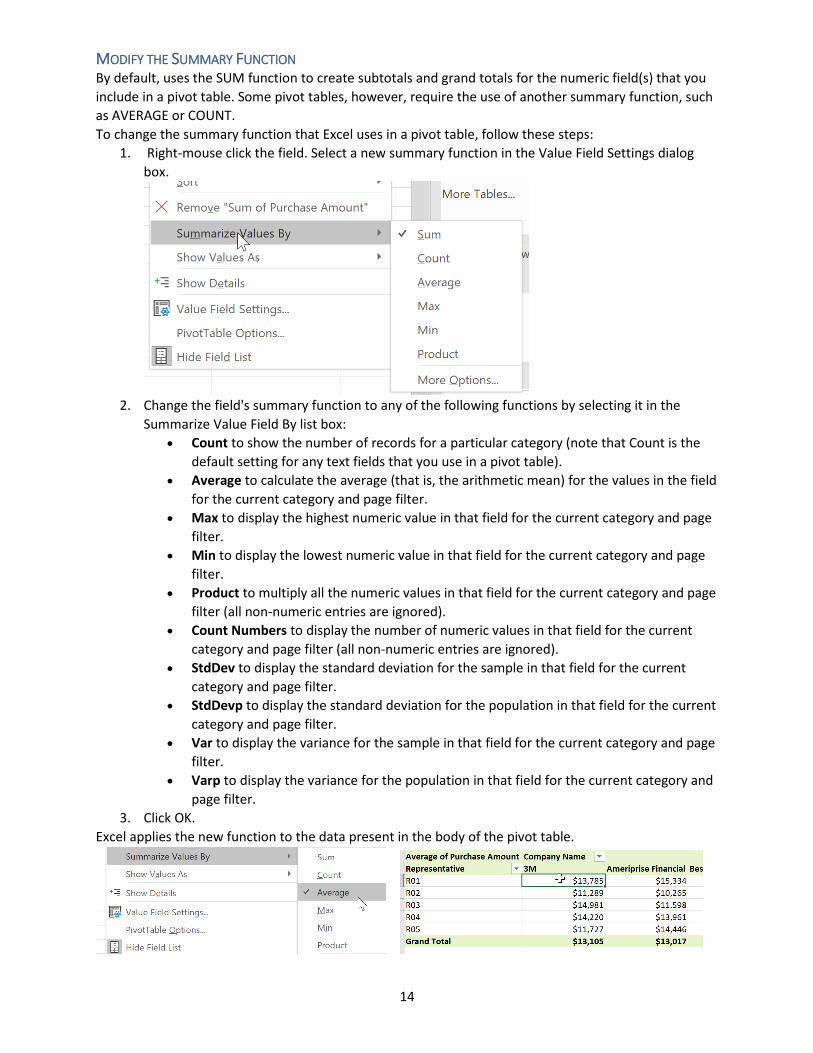
MODIFY THE SUMMARY FUNCTION By default, uses the SUM function to create subtotals and grand totals for the numeric field(s) that you include in a pivot table. Some pivot tables, however, require the use of another summary function, such as AVERAGE or COUNT. To change the summary function that Excel uses in a pivot table, follow these steps:

1. Right-mouse click the field. Select a new summary function in the Value Field Settings dialog box.

2. Change the field's summary function to any of the following functions by selecting it in the

Summarize Value Field By list box: • Count to show the number of records for a particular category (note that Count is the

default setting for any text fields that you use in a pivot table). • Average to calculate the average (that is, the arithmetic mean) for the values in the field

for the current category and page filter. • Max to display the highest numeric value in that field for the current category and page

filter. • Min to display the lowest numeric value in that field for the current category and page

filter. • Product to multiply all the numeric values in that field for the current category and page

filter (all non-numeric entries are ignored). • Count Numbers to display the number of numeric values in that field for the current

category and page filter (all non-numeric entries are ignored). • StdDev to display the standard deviation for the sample in that field for the current

category and page filter. • StdDevp to display the standard deviation for the population in that field for the current

category and page filter. • Var to display the variance for the sample in that field for the current category and page

filter. • Varp to display the variance for the population in that field for the current category and

page filter. 3. Click OK.

Excel applies the new function to the data present in the body of the pivot table.

15

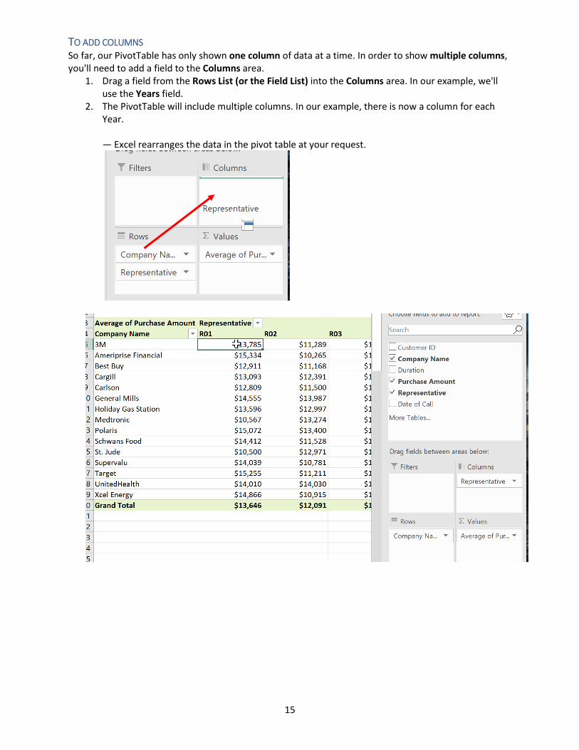
TO ADD COLUMNS So far, our PivotTable has only shown one column of data at a time. In order to show multiple columns, you'll need to add a field to the Columns area.

1. Drag a field from the Rows List (or the Field List) into the Columns area. In our example, we'll use the Years field.

2. The PivotTable will include multiple columns. In our example, there is now a column for each Year. — Excel rearranges the data in the pivot table at your request.

16

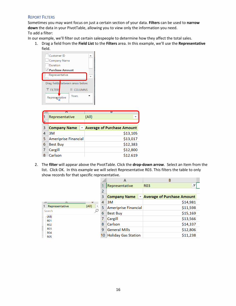
REPORT FILTERS Sometimes you may want focus on just a certain section of your data. Filters can be used to narrow down the data in your PivotTable, allowing you to view only the information you need. To add a filter: In our example, we'll filter out certain salespeople to determine how they affect the total sales.

1. Drag a field from the Field List to the Filters area. In this example, we'll use the Representative field.

2. The filter will appear above the PivotTable. Click the drop-down arrow. Select an Item from the list. Click OK. In this example we will select Representative R03. This filters the table to only show records for that specific representative.

17

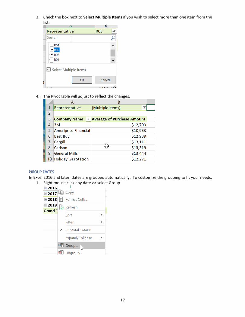
3. Check the box next to Select Multiple Items if you wish to select more than one item from the list.

4. The PivotTable will adjust to reflect the changes.

GROUP DATES In Excel 2016 and later, dates are grouped automatically. To customize the grouping to fit your needs:

1. Right mouse click any date >> select Group

18

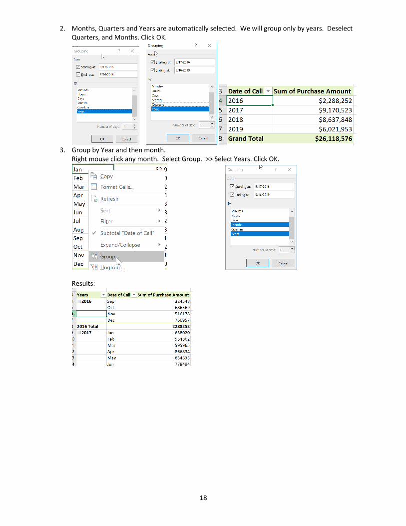
2. Months, Quarters and Years are automatically selected. We will group only by years. Deselect Quarters, and Months. Click OK.

3. Group by Year and then month.

Right mouse click any month. Select Group. >> Select Years. Click OK.

Results:

19

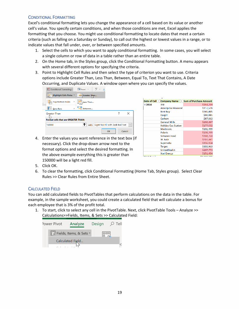
CONDITIONAL FORMATTING Excel's conditional formatting lets you change the appearance of a cell based on its value or another cell's value. You specify certain conditions, and when those conditions are met, Excel applies the formatting that you choose. You might use conditional formatting to locate dates that meet a certain criteria (such as falling on a Saturday or Sunday), to call out the highest or lowest values in a range, or to indicate values that fall under, over, or between specified amounts.

1. Select the cells to which you want to apply conditional formatting. In some cases, you will select a single column or row of data in a table rather than an entire table.

2. On the Home tab, in the Styles group, click the Conditional Formatting button. A menu appears with several different options for specifying the criteria.

3. Point to Highlight Cell Rules and then select the type of criterion you want to use. Criteria options include Greater Than, Less Than, Between, Equal To, Text That Contains, A Date Occurring, and Duplicate Values. A window open where you can specify the values.

4. Enter the values you want reference in the text box (if

necessary). Click the drop-down arrow next to the format options and select the desired formatting. In the above example everything this is greater than 150000 will be a light red fill.

5. Click OK. 6. To clear the formatting, click Conditional Formatting (Home Tab, Styles group). Select Clear

Rules >> Clear Rules from Entire Sheet. CALCULATED FIELD You can add calculated fields to PivotTables that perform calculations on the data in the table. For example, in the sample worksheet, you could create a calculated field that will calculate a bonus for each employee that is 3% of the profit total.

1. To start, click to select any cell in the PivotTable. Next, click PivotTable Tools – Analyze >> Calculations>>Fields, Items, & Sets >> Calculated Field:

20

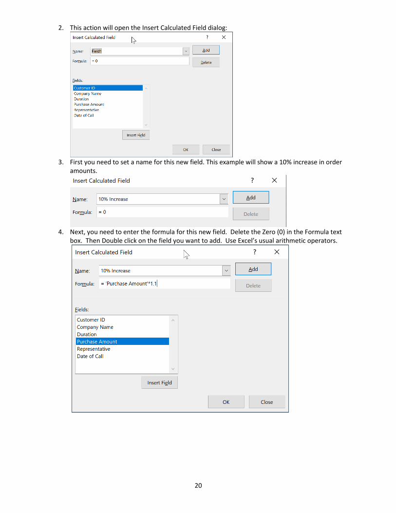
2. This action will open the Insert Calculated Field dialog:

3. First you need to set a name for this new field. This example will show a 10% increase in order

amounts.

4. Next, you need to enter the formula for this new field. Delete the Zero (0) in the Formula text

box. Then Double click on the field you want to add. Use Excel’s usual arithmetic operators.

21

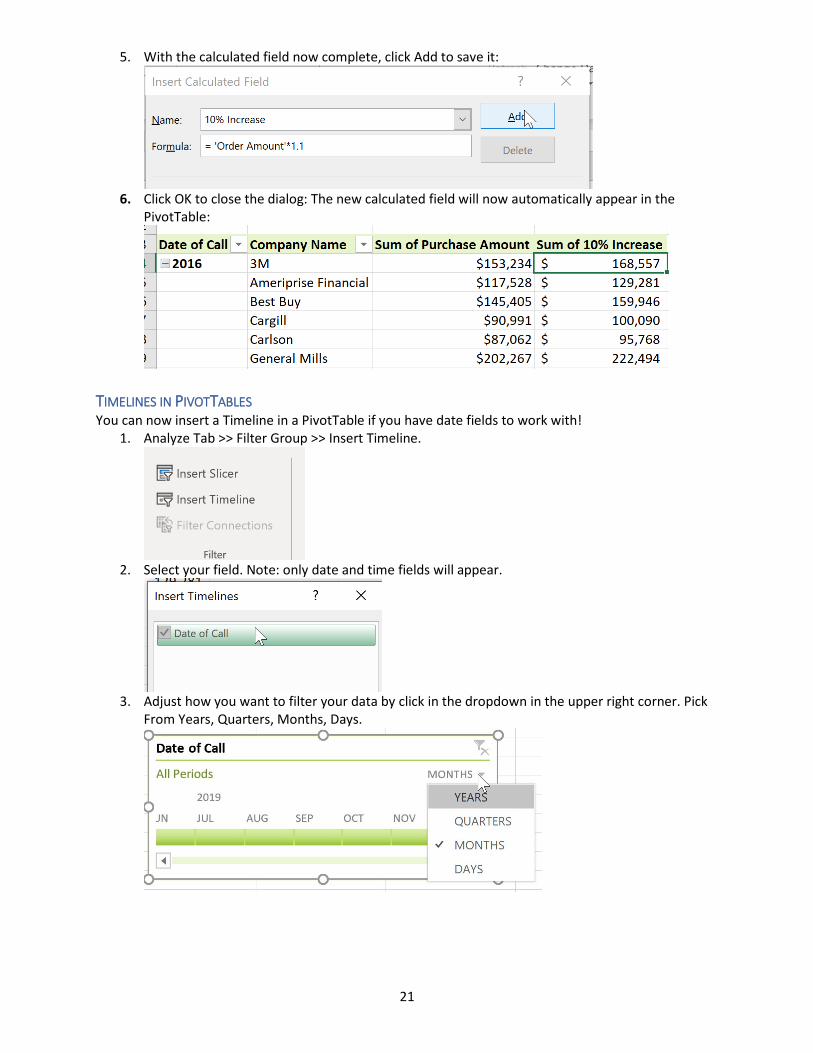
5. With the calculated field now complete, click Add to save it:

6. Click OK to close the dialog: The new calculated field will now automatically appear in the

PivotTable:

TIMELINES IN PIVOTTABLES You can now insert a Timeline in a PivotTable if you have date fields to work with!

1. Analyze Tab >> Filter Group >> Insert Timeline.

2. Select your field. Note: only date and time fields will appear.

3. Adjust how you want to filter your data by click in the dropdown in the upper right corner. Pick

From Years, Quarters, Months, Days.

22

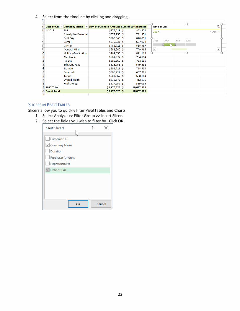
4. Select from the timeline by clicking and dragging.

SLICERS IN PIVOTTABLES Slicers allow you to quickly filter PivotTables and Charts.

1. Select Analyze >> Filter Group >> Insert Slicer. 2. Select the fields you wish to filter by. Click OK.

23

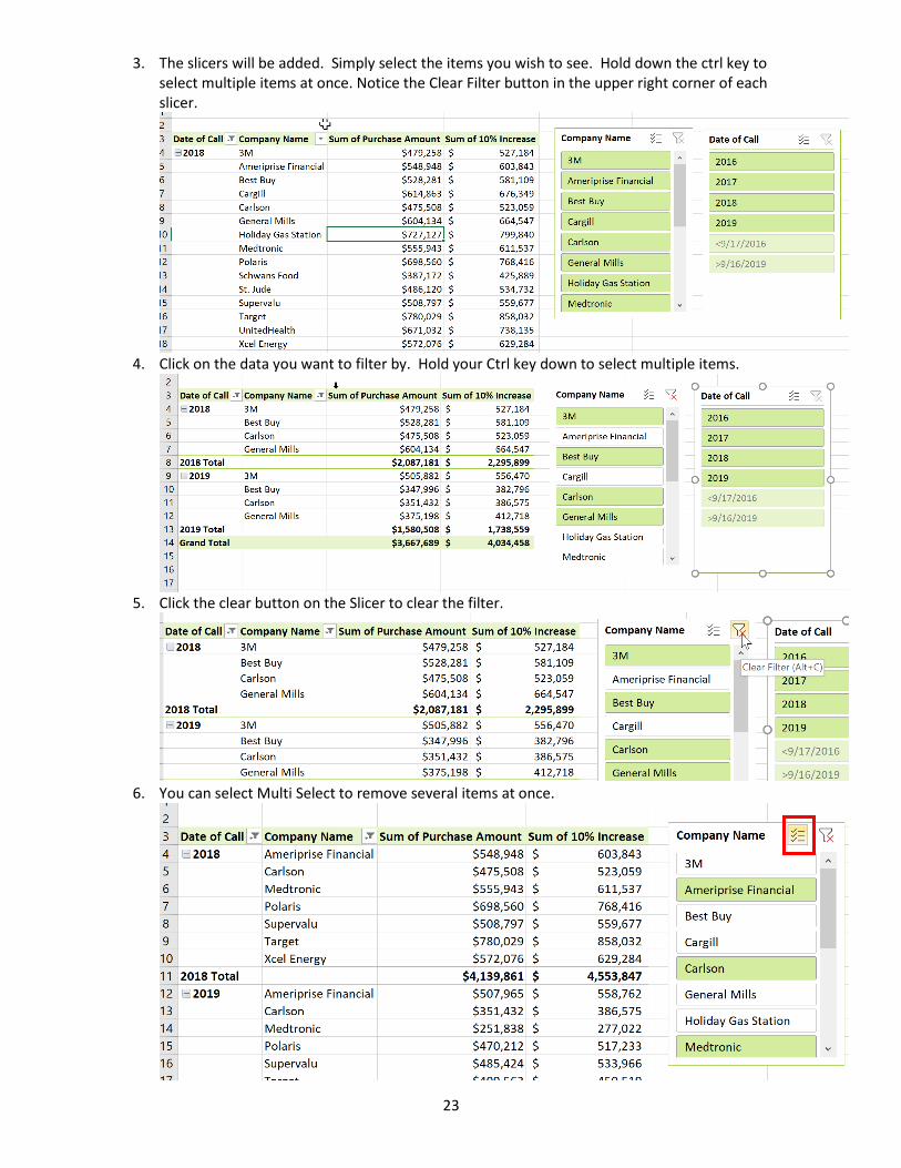
3. The slicers will be added. Simply select the items you wish to see. Hold down the ctrl key to select multiple items at once. Notice the Clear Filter button in the upper right corner of each slicer.

4. Click on the data you want to filter by. Hold your Ctrl key down to select multiple items.

5. Click the clear button on the Slicer to clear the filter.

6. You can select Multi Select to remove several items at once.

24

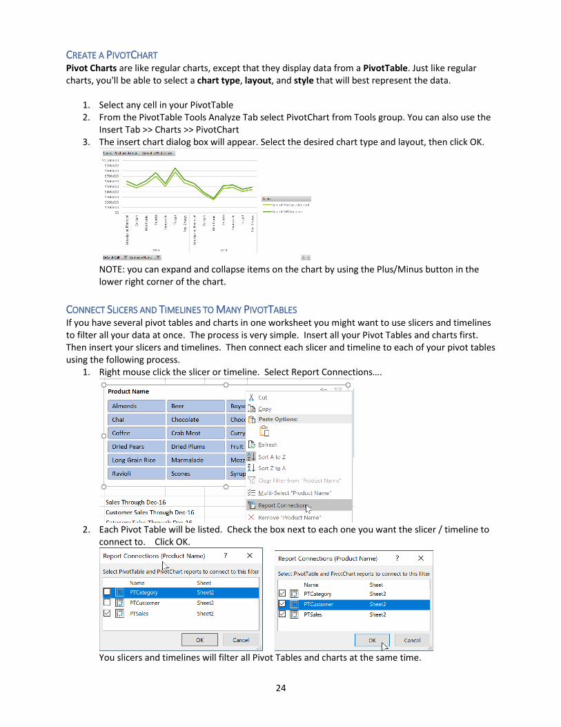
CREATE A PIVOTCHART Pivot Charts are like regular charts, except that they display data from a PivotTable. Just like regular charts, you'll be able to select a chart type, layout, and style that will best represent the data.

1. Select any cell in your PivotTable 2. From the PivotTable Tools Analyze Tab select PivotChart from Tools group. You can also use the

Insert Tab >> Charts >> PivotChart 3. The insert chart dialog box will appear. Select the desired chart type and layout, then click OK.

NOTE: you can expand and collapse items on the chart by using the Plus/Minus button in the lower right corner of the chart.

CONNECT SLICERS AND TIMELINES TO MANY PIVOTTABLES If you have several pivot tables and charts in one worksheet you might want to use slicers and timelines to filter all your data at once. The process is very simple. Insert all your Pivot Tables and charts first. Then insert your slicers and timelines. Then connect each slicer and timeline to each of your pivot tables using the following process.

1. Right mouse click the slicer or timeline. Select Report Connections….

2. Each Pivot Table will be listed. Check the box next to each one you want the slicer / timeline to

connect to. Click OK.

You slicers and timelines will filter all Pivot Tables and charts at the same time.

25

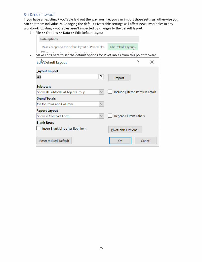
SET DEFAULT LAYOUT If you have an existing PivotTable laid out the way you like, you can import those settings, otherwise you can edit them individually. Changing the default PivotTable settings will affect new PivotTables in any workbook. Existing PivotTables aren’t impacted by changes to the default layout.

1. File >> Options >> Data >> Edit Default Layout

2. Make Edits here to set the default options for PivotTables from this point forward.

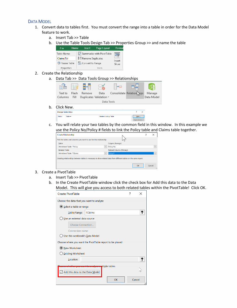
DATA MODEL 1. Convert data to tables first. You must convert the range into a table in order for the Data Model

feature to work. a. Insert Tab >> Table b. Use the Table Tools Design Tab >> Properties Group >> and name the table

2. Create the Relationship

a. Data Tab >> Data Tools Group >> Relationships

b. Click New.

c. You will relate your two tables by the common field in this window. In this example we

use the Policy No/Policy # fields to link the Policy table and Claims table together.

3. Create a PivotTable

a. Insert Tab >> PivotTable b. In the Create PivotTable window click the check box for Add this data to the Data

Model. This will give you access to both related tables within the PivotTable! Click OK.

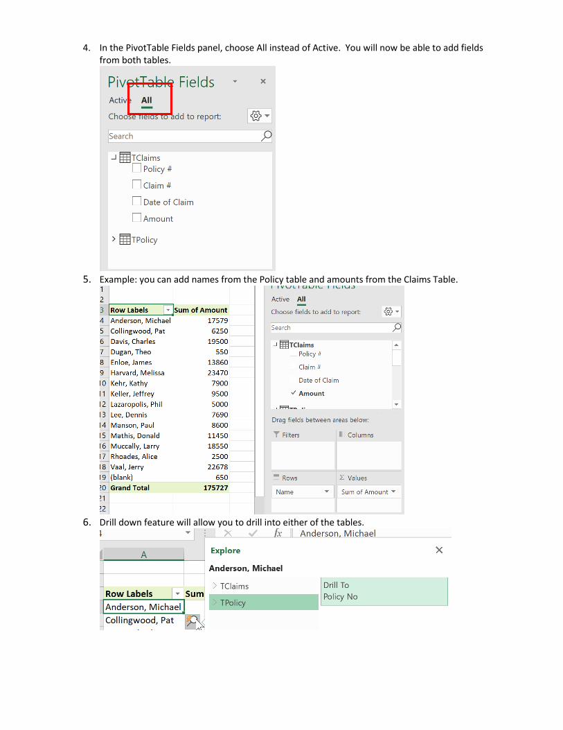
4. In the PivotTable Fields panel, choose All instead of Active. You will now be able to add fields from both tables.

5. Example: you can add names from the Policy table and amounts from the Claims Table.

6. Drill down feature will allow you to drill into either of the tables.