Excel 2010 Statistics - Columbia Business School · PDF file1 MS Excel 2010 for Business Statistical Applications 1 Learning Aims In this second part of the introduction to Microsoft

1

MS Excel 2010 for Business Statistical Applications 1

Learning Aims In this second part of the introduction to Microsoft Excel for Business, we will explore some of the statistical capabilities of Excel. The main learning aims are: Use of the Data Analysis ‘add-ins’, and histogram construction; Use of the Descriptive Statistics tool, including references between worksheets; Using statistical functions to calculate individual descriptive statistics; Short preview of variance and the covariance matrix in Excel.

Introduction

Spreadsheets provide functions for doing calculations. Click on a blank cell, and then on the fx button to the left of the formula bar (or go to the left end of the Formulas tab) to Insert Function, and examine the various function categories from the central drop-down list; select Statistical. You will then see many statistical functions listed down the left side of the dialog box.

In addition to providing statistical functions, Excel is structured so that you can also load extensions – programs that perform operations additional to the functions that come in the standard version of Excel. Some of these extensions are for statistics and are sold as part of Excel (but you can choose to save disk space by not installing them, if you are unlikely to use them). Others, such as Palisade’s @Risk, for

building statistical simulation models, are sold independently. This note will make use of the Data Analysis ‘ToolPak’ add-ins, which come with Excel. If you have Excel on your own machine, it’s probably installed already; you will see how to check this on the next page.

1 This note was written by Paul G. Ellis, Teaching and Research Co-ordinator, Management Science and Operations, London Business School. [email protected] No part of this publication may be reproduced, stored in a retrieval system, used in a spreadsheet, or transmitted in any form or by any meanselectronic, mechanical, photocopying, recording, or otherwisewithout the permission of the author. Copyright 2007, 2011. Earlier Excel2003 version available via the author.

2

DISTRIBUTION OF HEIGHTS

0

2

4

6

8

10

12

Heights (m)

FREQ

UENC

Y

Statistical Tools in the Data Analysis ‘ToolPak’ First open the spreadsheet Height.xlsx (available on Portal Course Rooms, some Admit sites and London campus network Q:\Students\BusStat\Excel…; also illustrated on the back page of this note). This file gives you data about two imaginary groups of students. One group is a single class of Business students. The other is a sample taken at random, from all of a school's students2. You may suspect that there are subtle differences in the characteristics of the two groups. Before examining the data, let us see how to graph it so as to indicate clearly the numbers of observations falling within neighbouring ranges of values – i.e. in a histogram. First, however, we need to access the Data Analysis ‘ToolPak’, (a set of add-in programs) that provides a convenient way of assembling the data to draw histograms, along with a number of other useful statistical tools.

Data Analysis Add-in

Click on an empty cell to ensure nothing else is selected, then click the Data tab to see Data Analysis at the right end. If it’s not there, then see pp. 19-21 in Excel_2010_Basics.pdf to see how to link the Analysis ToolPak-VBA into Excel, via File/Options/Add-Ins/Manage: Excel Add-ins/Go, select both ToolPak add-

ins and press OK, so that you can work through these notes using Data Analysis. On your own computer, you should only need to do this once, but if the ToolPaks are not listed in your add-ins, you will need to get them from the original installation disk.

Histograms

The first of these Data Analysis tools that we shall use allows us to draw a histogram – a frequency distribution of the data. Let us say that with the data about heights, we are interested in the number of business students whose heights are ‘between’ 1.5m and 1.55m, the number between 1.55m and 1.6m, and so on until we reach the number between 1.85m and 1.9m (as

will be defined more precisely, below). If we can draw a graph of these numbers we can gain an impression of the distribution of heights represented by the data. From the Data tab, and Data Analysis, we can do this by selecting Histogram from the available list of analysis tools. This function will create a table from which a histogram of the

2 If you’ve done no statistics as yet, be aware that complete groups (‘populations’) are treated in a slightly different way from samples (i.e. samples are approximate representatives of populations) and Excel uses slightly different functions for calculations of their characteristics (e.g. VAR.P and VAR.S for their respective ‘variances’: ways of measuring the amount of variation in some characteristic of groups).

3

heights can be drawn. For this exercise you only need two of the fields in the window that will appear; each takes the address of a range of cells. The input range is the range of cells containing the heights: A18:A72. You can either type this into the input range field (notice that you can put either a colon ‘:’ or two horizontal dots ‘..’ between the two end-cell addresses of the range), or you can click in the input range field and then highlight the cells from A18 to A72 with the mouse. Do not hit Enter until the dialog box is complete; also note that after inputting range addresses, Excel makes them absolute (e.g. $A$18; see the Excel 2010 Basics note for more on relative and absolute addressing). Now click the ‘radio button’ next to the words Output Range. This tells the spreadsheet to put the result into the same worksheet. The result will not be a graph, but rather the frequency table that summarises the data, and from which a graph can then be drawn to illustrate this tabulation of the data. Click in the Output Range field and either type in an address such as A100, where the top left corner of the frequency table is to be placed, or just click that cell (easier to reach if you click on the Collapse Dialog button: to obtain freedom to navigate, and after selecting A100, click it again). Leave the other fields in the dialog box blank for the time being, and click OK. Now look at the result in cells A100 to B108. The left hand

column, titled Bin (which can be renamed if necessary to something more appropriate – e.g. ‘Height ranges’) contains a set of heights (representing the boundaries of the ranges) chosen by the program. The right hand column shows the number of students whose heights fall between the height in the bin range and the preceding one. So, in this case, one student has a height less than or equal to 1.508m (you may need to increase the number of decimals in the original data column to verify this), three have heights that could be expressed as: (1.508m < Height <= 1.561m), and so

on. Notice the signs are first ‘<’ and then ‘<=’; think for a moment why these should both be needed (NB Excel doesn’t recognise ‘< ‘). Using the histogram function in this simple manner results in Excel calculating range boundaries between each successive group (or bin) of heights – that rarely coincide with more natural boundaries for these ‘class intervals’. Note that if you are dealing with a small amount of data, the choice of boundaries can make a significant difference to the way that the histogram of the data appears.

Choose your own class intervals by defining a bin range: A suitable set of class intervals could be every 0.05m from 1.5m to 2m. Place the numbers 1.5 and 1.55 in cells A86 to A87, then select these two cells together, and see how the cursor becomes a black cross (called the fill handle) when it lies over the lower right corner of the lower selected cell (here, A87). This fill handle can be used to quickly create a series of values by dragging down, here to cell A96, taking the bin range to 2.0. Now try producing the frequency table again but this time put the range A86:A96 into the field marked bin range and also tick Chart Output in the lower left corner of the histogram dialog box3. Note that Excel will give you a warning message before you let it put

your new histogram data in place of the old. You will find that the resulting data appears with a different

3 If you find that Excel refuses to draw the chart, claiming that the workbook is ‘shared’, the selected add-in was probably ToolPak rather than

ToolPak-VBA; link in the other ToolPak add-in as well, or simply continue and choose to place the output in a new workbook, in which case you can then select all the contents and copy them back into the original worksheet, if you wish.

4

set of class intervals, which you may find easier to work with in practice. The chart should also appear nearby, as follows.

Try clicking on parts of the chart to change it: e.g., first select the chart and drag down from the middle of the lower edge to get a better view of the bars indicating the frequencies of each bin range of heights. Click on the title and make it more descriptive. Try a left-click on the x-axis and use Format Axis (this can be tricky, as the tip of the cursor needs to be precisely on the line) to

change e.g. the x-axis labels’ alignment. Make the bar chart look more like a proper histogram, by reducing the gaps between the bars (right-click on a bar and choose Format Data Series….) If you’re concerned with detail, you might also show how the bin/frequency values are defined (e.g. 1.5m < Height <= 1.55m) by indicating this in the Height column of the table (as shown for two of the bin ranges), so that it then appears on the x-axis. Other alternatives can be reached, more easily, after clicking on the chart so that the green group-tab Chart Tools appears, offering Design, Layout and Format options.

If you like, you could practise this further by creating another histogram, for the students’ weights listed in Column B. Play with the various options to make it more interesting than the default graph.

5

Descriptive Statistics Tool When first examining some new statistics it is often helpful to start with an overview. Graphing a distribution, as we have just done, is one way, and it often gives a quick idea of means, modes and a sense of the dispersion in the data. In particular, it can indicate the shape of a distribution. Another way to get a quick overview is to compute a range of commonly-used measures. It is worth knowing that the Data Analysis tools include a facility to produce such a range of descriptive statistics all in one go. We will apply this approach to the data on the right-hand side of the sheet – that is the data about the sample taken from across a university. (Remember that the BS class data, on the other hand, is not a sample, but a population: one complete BS Class.) Later we will look at other cases where one might only need one or two statistics, such as a mean and a standard deviation4, which could be calculated individually using standard Excel functions. In Data Analysis choose Descriptive Statistics. Take as the input range F18:H82, which takes in three columns of data about the sample. Click on the small square labelled Summary statistics, to tell Data Analysis what output you require. This time we will put the output into a new worksheet: So far, we’ve made little mention of the fact that when you open an Excel file, you open an Excel workbook, which can contain several worksheets indicated by tabs (Sheet1, Sheet2, etc.) along the bottom of the spreadsheet screen. Each worksheet can contain different data, but has a similar structure and has addresses starting at a cell ‘A1’ in the same way. One workbook can contain many worksheets. You can rename the sheets merely by double-clicking on the sheet-names on the tabs near the bottom of the screen. Move between sheets by clicking on the tab naming the sheet you wish to access, or by using the keyboard Ctrl+PageUp and Ctrl+PageDown keys.

To illustrate this use of alternative worksheets, instead of selecting an output range for our descriptive statistics, we will choose to put the result in a new worksheet ply (i.e. in a new worksheet in the same workbook (i.e. file)). When you have chosen this option via a radio button, and clicked OK, then look at the bottom of your screen. Where you initially saw just the words Heights & Weights (the name of the original worksheet), you should now be in the new worksheet, probably called ‘Sheet1’, but if you’re not in it, move to it as described in the previous paragraph. As the names in the output Columns may be partially overwritten by numbers, select the whole table and, in the Home tab,

click on Format and Autofit Column Width to make them fully visible; if necessary, adjust the screen via the View tab and Zoom. Double click on the tab, and name this new worksheet, which displays data about the three columns – more analysed data than you may really need. The objective of this exercise is simply to make you aware of the tool and to emphasise the use of multiple worksheets. The worksheets can be treated as entirely separate, or sometimes it can be useful to work across multiple worksheets, as shown briefly in the next section.

4 Standard deviation (SD) is another measure of the variability of a set of values – an average of how much the values differ from the mean value, and is closely related to variance, mentioned in an earlier footnote. SD is the positive square root of variance. Note also that Excel uses the word ‘Average’ (e.g. for the function to calculate an average), but Data Analysis uses the similar word ‘Mean’.

6

References between Worksheets

It is possible to refer from a cell in one worksheet to a cell in a different worksheet, much as it is possible to refer between cells within a single worksheet. As an example, let us look at the mean (another term for ‘average’) and median values for column F of the original worksheet – that is for the heights of the sample of students. The mean of these heights appears in cell B3 of the new worksheet created in the previous section (Sheet1), and the median appears further down, in cell B5. If we are interested in whether the heights follow a bell-shaped (so-called ‘Normal’) distribution, we might want to look at the difference between these two values, as one possible indicator of non-normality.

First, return to the original Heights & Weights worksheet. Now we want to put into cell F85 the mean of column F, and in F86 the difference between it and the median (move out of the way any graph or table you might have already placed over these cells). Type ‘Mean’ into E85 and ‘Difference’ into E86. These are simply labels to remind us that row 85 will hold means while row 86 will show the differences between medians and means.

Now click cell F85 and type ‘=’ to show that you are about to type in a formula. Next click the tab for the Sheet1 worksheet, and click cell B3 in that worksheet. When you have done this, you should see ‘=Sheet1!B3’ appearing in the formula bar at the top of the screen. Press Enter and you should return automatically to the Heights & Weights sheet, while Excel pastes the result directly into cell F85 of this sheet. The technique for referring to cells is basically the same whether or not the cell and its reference are in the same worksheet, the only difference being the need to click the tab of the 2nd worksheet, and the cell address being extended to include the worksheet name, followed by an exclamation mark.

Put into cell F86, of the Heights & Weights worksheet, the difference between the mean and the median that are located in the Descriptive Statistics table on the other worksheet, by the same method. The resulting formula in cell F86 should read ‘=Sheet1!B3-Sheet1!B5’. If the result is just 0 (or -0), try increasing the number of decimal places using either

the Increase Decimal button (Home tab, Number group icon or via Format/Format Cells….)

7

Using individual Statistical Functions You will recall that we started out with an interest in the differences between two groups of students represented in the data file Height.xlsx. Now that we have seen how to gain overviews via histograms and summary statistics we can examine ways of obtaining the values for specific individual statistical measures, either by using the Insert Function method plus the input data (also called arguments), or by keying the function name directly into a cell, together with the arguments. Initially we are interested in the heights. For the BS students, we shall replace the question marks on the data sheet by putting the function for their mean (i.e., average) height in cell B9, likewise for the variance of their heights, in cell C9, and for the standard deviation of their heights in cell D9.

Click first on the target cell, B9. Go via the fx button and select the category Statistical to reach the function to calculate the mean (called Average by Excel) and hit OK; If the Insert Function dialog box that then appears hides the height data from view, then again (as on p. 3) you can use the Collapse Dialog button: to reach the data. Once the data’s cell references have been selected, click the coloured square once more, to return to the dialog box and see the result previewed before you hit OK, allowing you to accept or correct it. You should obtain the average of 1.72701924

(metres). Notice that in calculating the average, all you needed to do was tell the function which overall range of items to average. Even if there are gaps (as there will be in the Weight statistics) it will count up automatically to see how many items the total value needs to be divided by, to give the true average. Using the Insert Function dialog box again, you can also complete the entries in C9 and D9; (the corresponding functions for these statistics can also handle blank spaces, where data is missing) but remember when you select the two functions for the variance and standard deviation of the heights, you are dealing in this case with a population, not a sample, and should use VAR.P and STDEV.P for populations, while VAR.S and STDEV.S are for samples (data in the right side columns, F to I), as mentioned earlier, in Footnote 2. Next, try doing the height statistics for the Random sample, on the right of the data file, by entering the formulas and their arguments directly, in G9 to I9: Simply type =Average( . Then key in, or use the mouse to select, the cell references of the data to be averaged: F18:F82 (or use the easy method: click on F18, then hold down both the Shift and Ctrl keyboard buttons, and hit the arrow that goes in the direction of the data; if it’s in a single connected row or column, it will all be selected in a single step), then finish with the right parenthesis ‘)’ and OK. If you are not sure how to type in the other formulas (for H9 and I9), try using the contents of

8

cells C9 and D9 as guides, but don’t forget the above-mentioned differences (sample vs population); you can also read the hints on the various functions’ dialog boxes when raised via the Insert Function fx button. A better way to address data can be to refer to it as a named block, by giving it a range name. The advantage is that firstly you (or, more importantly, someone unfamiliar with the spreadsheet) can read the formulas more easily; and secondly, you can address the data using the range name, rather than cell addresses. We’ll try this for the final block of calculations, the weight statistics for the random sample5.

Select G18 to G82, go to the Formulas tab, Define Name and type in the top line of the dialog box the name Sample_weights (note the underscore; hyphens and gaps not accepted) and click OK. Find the name in the Name Box, to the left of the formula bar. If the Sample_weights data is still selected, first click anywhere else in the sheet (to lose the selection), then select the name in the Name Box and see the whole defined range of data being reselected. Now you can insert a formula somewhere and, instead of the cell addresses, start to key the range-name of the data into the function name, e.g. =average(Sa and you

should see the range name appear as shown below; at which point you only need to select the correct range name using an arrow key, then press the Tab key for the whole name to be entered; complete the argument(s) (none in this case) and with the final parenthesis to complete the function, you can press OK. This also provides a neat way to move about large spreadsheets. If there are points well away from the “Home” corner (cells close to A1), simply select a cell near where you might need to reach fairly frequently, define a name for that one cell, and by later selecting the name from the Name Box, you can jump to that point directly. Now we have used statistical functions individually, we can see that going via the Descriptive Statistics, earlier, was in fact a fairly cumbersome way of putting the mean and median of a data set into a worksheet. There is no advantage in using the descriptive statistics tool unless you want more than one or two of the statistics, e.g. a quick overview before you know where you need to focus. But now

we can do so to illustrate an important point. For comparison, recalculate the mean of the column F data in cell G85 using the fx button. You should find that the two cells F85 and G85 contain the same result. Make sure that G85 has the correct formula by comparing its contents and those of G9 in the formula bar.

Now change the value of cell F82 from 1.80 to 1.70. You are altering part of your input data. You should notice that the mean in cell G85 changes, but the mean in cell F85 does not! This is because of a subtle but important difference in the way that the two means are calculated.

5 Because of the gaps in the weight data you may find it easier to simply key in the initial and final cell references, or use the mouse (using the Shift and Ctrl keys when there are n gaps now needs the arrow key to be used (2n+1) times). =

9

When you selected Data Analysis… to do Descriptive Statistics you asked Excel to do a single, one-off calculation. It puts the results of that calculation into various cells (in this case the ‘Sheet1’ worksheet shown here again) but once they are in those cells, they remain as constants6. Conversely, when you use an Excel formula such as ‘=AVERAGE(…)’, you set up one cell as being dependent on others (the inputs). Therefore when the data cell (or set of cells) changes, the destination (result) cell changes too. The importance of this becomes clear when one considers a spreadsheet that will be periodically updated, with automatic recalculation being required. (Reset cell F82 to 1.79657 ; it only showed in Height.xlsx as 1.80 as it was formatted to 2 decimal places.)

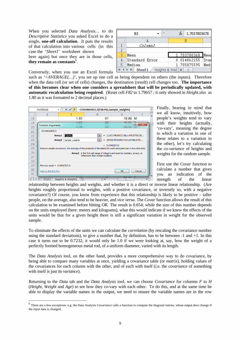
Finally, bearing in mind that we all know, intuitively, how people’s weights tend to vary with their heights (actually, ‘co-vary’, meaning the degree to which a variation in one of these relates to a variation in the other), let’s try calculating the co-variance of heights and weights for the random sample. First use the Covar function to calculate a number that gives you an indication of the strength of the linear

relationship between heights and weights, and whether it is a direct or inverse linear relationship. (Are heights roughly proportional to weights, with a positive covariance, or inversely so, with a negative covariance?) Of course, you know from experience that this relationship is likely to be positive – taller people, on the average, also tend to be heavier, and vice versa. The Covar function allows the result of this calculation to be examined before hitting OK. The result is 0.654; while the size of this number depends on the units employed (here: meters and kilograms), what this would indicate if we knew the effects of the units would be that for a given height there is still a significant variation in weight for the observed sample. To eliminate the effects of the units we can calculate the correlation (by rescaling the covariance number using the standard deviations), to give a number that, by definition, has to be between -1 and +1. In this case it turns out to be 0.7232; it would only be 1.0 if we were looking at, say, how the weight of a perfectly formed homogeneous metal rod, of a uniform diameter, varied with its length. The Data Analysis tool, on the other hand, provides a more comprehensive way to do covariance, by being able to compare many variables at once, yielding a covariance table (or matrix), holding values of the covariances for each column with the other, and of each with itself (i.e. the covariance of something with itself is just its variance). Returning to the Data tab and the Data Analysis tool, we can choose Covariance for columns F to H (Height, Weight and Age) to see how they co-vary with each other. To do this, and at the same time be able to display the variable names in the output, we need to ensure the variable names are in the row

6 There are a few exceptions: e.g. the Data Analysis Covariance calls a function to compute the diagonal entries, whose output does change if the input data is changed.

10

immediately above the data. We can simply copy the table and overwrite the lines of hyphens that lie between the variable names and the first row of data. Notice that one of the matrix entries is the almost same as the output of the Covar function, but not quite the same. If you examine the results closely you will find that while the Excel Covar function uses VAR.S To calculate the covariances, the Data Analysis tool’s Covariances (and thus the variance resulting from calculating a variable’s covariance with itself) uses the VAR.P function. Finally: Why might some of the table entries be left blank?

Now that you have finished this note, if you have any outstanding questions, or would like to suggest improvements that could help make these notes more useful, please feel free to email me with queries or suggestions: [email protected]

11

Appendix – Summary of Excel Tips and Tricks for Statistics7

Statistical Tools in the Data Analysis ToolPak/Data Analysis Add-ins If the menu entry Data Analysis… fails to appear at the right end of the Data Tab, then see pp. 19-21 in Excel_2010_Basics.pdf to see how to link the Analysis ToolPak-VBA into Excel, via File/Options/Add-Ins/Manage: Excel Add-ins/Go, select both ToolPak add-ins and press OK.

Histograms Creating arithmetic series (e.g. for quickly setting up regular inputs for a table, such s bin ranges): Put two numeric values in neighbouring cells, select both, and drag using the “fill handle” in the lower right corner of the cell (cursor changes to a small cross, when it’s ready to drag out the series); result is a continuation of the implied arithmetic series e.g. 12 and 14 in two cells, selected and using the fill handle a continuation of the series with 16 18 20 etc., in the row or column of cells following. Range separators generally, e.g. the colon in “A18:A72”, can also be two horizontal dots (full stops) “A18..A72”. To format data elements on a graph, double click on the data points or bars etc.

Descriptive Statistics Tool To make visible any cell contents hidden by overlapping cells, go to Home Tab and click on Format and AutoFit Column Width (but beware lengthy formulas or text) TIP Ensure there is no textual information mixed in with numeric data supplied to the Data

Analysis tool, else it will return an error message. References between Worksheets To generate a formula referring to the contents of another worksheet in the same workbook (i.e. in the same .xlsx file), after typing ‘=’ and perhaps other ‘local’ parts of the formula, click on the tab for the other worksheet, select the required cells, and hit Enter, returning you to the original worksheet with the selected element in place. Using individual Statistical Functions While the results of using an individual statistical function will adjust after changing an input value, note that the Data Analysis tools mostly do a one-time-only calculation. If an input value changes, a Data Analysis calculation must usually be rerun (but see footnote 6). TIP To jump between specific widely-separated points on a spreadsheet, on a frequent basis, it’s

worth setting up a range name for a nearby cell, so you can jump via a selection made in the range-name box. This also works between the sheets.

7 See the Excel2010_Basics.pdf for a more comprehensive list of Excel Tips and Tricks.

12

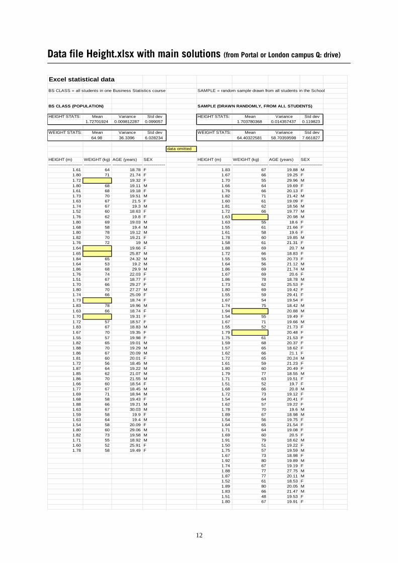
Data file Height.xlsx with main solutions (from Portal or London campus Q: drive) Excel statistical data

BS CLASS = all students in one Business Statistics course SAMPLE = random sample drawn from all students in the School

BS CLASS (POPULATION) SAMPLE (DRAWN RANDOMLY, FROM ALL STUDENTS)

HEIGHT STATS: Mean Variance Std dev HEIGHT STATS: Mean Variance Std dev1.72701924 0.009812287 0.099057 1.703780368 0.014357437 0.119823

WEIGHT STATS: Mean Variance Std dev WEIGHT STATS: Mean Variance Std dev64.98 36.3396 6.028234 64.40322581 58.70359598 7.661827

data omitted

HEIGHT (m) WEIGHT (kg) AGE (years) SEX HEIGHT (m) WEIGHT (kg) AGE (years) SEX------------------------- -------------------- ---------------------- ---------------- ------------------------- -------------------------- ---------------------- ----------------

1.61 64 18.78 F 1.83 67 19.88 M1.80 71 21.74 F 1.67 66 19.25 F1.72 19.32 F 1.70 55 29.96 M1.80 68 19.11 M 1.66 64 19.69 F1.61 68 19.18 F 1.76 66 20.13 F1.73 70 19.51 M 1.82 71 21.42 M1.63 67 21.5 F 1.60 61 19.09 F1.74 67 19.3 M 1.81 62 18.56 M1.52 60 18.63 F 1.72 66 19.77 M1.76 62 19.8 F 1.63 20.98 M1.80 69 19.03 M 1.63 55 18.6 F1.68 58 19.4 M 1.55 61 21.66 F1.80 78 19.12 M 1.61 58 19.6 F1.82 70 19.21 F 1.78 60 19.85 M1.76 72 19 M 1.58 61 21.31 F1.64 19.66 F 1.88 69 20.7 M1.65 25.87 M 1.72 66 18.83 F1.84 65 24.32 M 1.55 55 20.73 F1.64 53 19.2 M 1.64 56 21.12 M1.86 68 29.9 M 1.86 69 21.74 M1.76 74 22.03 F 1.67 69 20.6 F1.51 67 18.77 F 1.86 78 18.78 M1.70 66 29.27 F 1.73 62 25.53 F1.80 70 27.27 M 1.80 69 19.42 F1.74 66 25.09 F 1.55 59 29.41 F1.73 18.74 F 1.67 54 19.54 F1.83 78 19.96 M 1.74 75 18.42 M1.63 66 18.74 F 1.94 20.88 M1.70 19.31 F 1.54 55 19.49 F1.72 57 18.57 F 1.67 71 19.66 M1.83 67 18.83 M 1.55 52 21.73 F1.67 70 19.35 F 1.79 20.48 F1.55 57 19.98 F 1.75 61 21.53 F1.82 65 19.01 M 1.59 68 20.37 F1.88 70 19.29 M 1.57 65 18.62 F1.86 67 20.09 M 1.62 66 21.1 F1.81 60 20.01 F 1.72 65 20.24 M1.72 56 18.45 M 1.61 59 21.23 F1.87 64 19.22 M 1.80 60 20.49 F1.85 62 21.07 M 1.79 77 18.55 M1.86 70 21.55 M 1.71 63 19.51 F1.66 60 18.54 F 1.51 52 19.7 F1.77 67 18.45 M 1.68 66 20.8 M1.69 71 18.94 M 1.72 73 19.12 F1.68 58 19.43 F 1.54 64 20.41 F1.88 66 19.21 M 1.62 57 19.22 F1.63 67 30.03 M 1.78 70 19.6 M1.59 58 19.9 F 1.89 67 18.98 M1.63 64 19.4 M 1.54 56 19.75 F1.54 58 20.09 F 1.64 65 21.54 F1.80 60 29.06 M 1.71 64 19.08 F1.82 73 19.58 M 1.69 60 20.5 F1.71 55 18.92 M 1.91 79 18.62 M1.60 52 25.91 F 1.50 51 19.22 F1.78 58 19.49 F 1.75 57 19.59 M

1.67 73 18.98 F1.92 80 19.89 M1.74 67 19.19 F1.88 77 27.75 M1.87 77 20.11 M1.52 61 18.53 F1.89 80 20.05 M1.83 66 21.47 M1.51 48 19.53 F1.80 67 19.91 F