Examples of Deviation from Hardy-Weinberg Equilibrium AAAaaa Generation 10.640.320.04 Generation 20.630.330.04 Generation 30.640.3150.045 Generation 40.650.310.04.

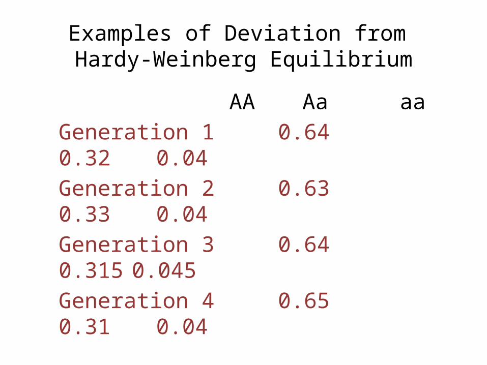
Examples of Deviation from Hardy-Weinberg Equilibrium

AAAa aa

Generation 1 0.640.32 0.04Generation 2 0.630.33 0.04Generation 3 0.640.315 0.045Generation 4 0.650.31 0.04

Is this population in HW equilibrium?If not, how does it deviate?What could be the reason?

Testing for Deviaton from Hardy-Weinberg Expectations

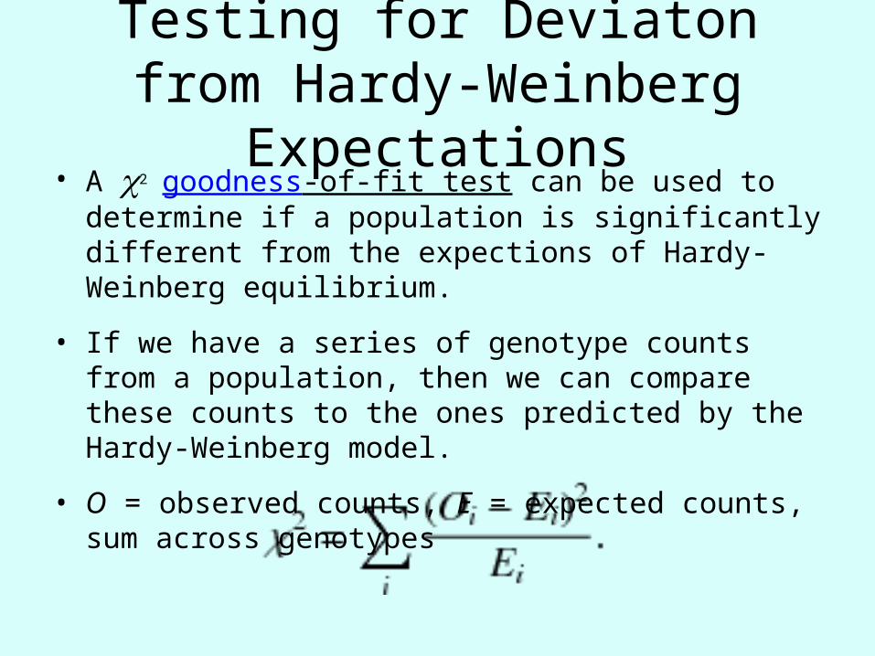
• A c2 goodness-of-fit test can be used to determine if a population is significantly different from the expections of Hardy-Weinberg equilibrium.

• If we have a series of genotype counts from a population, then we can compare these counts to the ones predicted by the Hardy-Weinberg model.

• O = observed counts, E = expected counts, sum across genotypes

Testing for Deviaton from Hardy-Weinberg Expectations

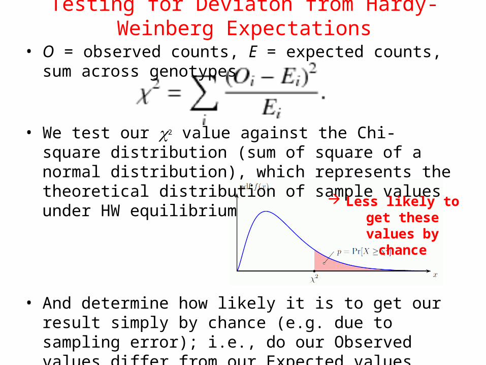
• O = observed counts, E = expected counts, sum across genotypes

• We test our c2 value against the Chi-square distribution (sum of square of a normal distribution), which represents the theoretical distribution of sample values under HW equilibrium

• And determine how likely it is to get our result simply by chance (e.g. due to sampling error); i.e., do our Observed values differ from our Expected values more than what we would expect by chance (= significantly different)?

• ?

Less likely to get these values by

chance

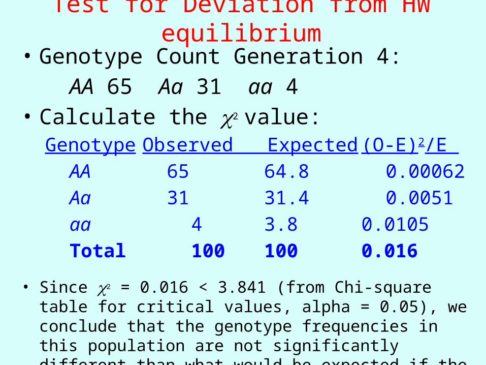
Test for Deviation from HW equilibrium• Genotype Count Generation 4:

AA 65 Aa 31 aa 4 • Calculate the c2 value:

Genotype Observed Expected (O-E)2/E AA 65 64.8 0.00062Aa 31 31.4 0.0051 aa 4

3.8 0.0105Total 100 100

0.016

• Since c2 = 0.016 < 3.841 (from Chi-square table for critical values, alpha = 0.05), we conclude that the genotype frequencies in this population are not significantly different than what would be expected if the population were in Hardy-Weinberg equilibrium.

• The chi-squared distribution is used because it is the sum of squared normal distributions

• Calculate Chi-squared test statistic• Figure out degrees of freedom• Select confidence interval (P-value)• Compare your Chi-squared value to the theoretical

distribution (from the table), and accept or reject the null hypothesis.– If the test statistic > than the critical value, the null hypothesis (H0

= there is no difference between the distributions) can be rejected with the selected level of confidence, and the alternative hypothesis (H1 = there is a difference between the distributions) can be accepted.

– If the test statistic < than the critical value, the null hypothesis cannot be rejected

Test for Significance of Deviation from HW Equilibrium

Degrees of Freedom is n – 1 = 2 alleles (p, q) -1 = 1

Testing for significance• The results come out not significantly different from HW

equilibrium

• This does not necessarily mean that genetic drift is not happening, but that we cannot conclude that genetic drift is happening

• Either we do not have enough power (not enough data, small sample size), or genetic drift is not happening

• Sometimes it is difficult to test whether evolution is happening, even when it is happening... The signal needs to be sufficiently large to be sure that you can’t get the results by chance (like by sampling error)

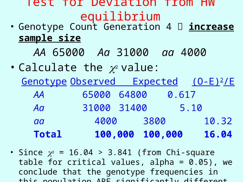
Test for Deviation from HW equilibrium• Genotype Count Generation 4 increase sample size

AA 65000 Aa 31000 aa 4000• Calculate the c2 value:

Genotype Observed Expected (O-E)2/E AA 65000 64800

0.617 Aa 31000 31400

5.10 aa 4000 3800 10.32 Total 100,000 100,000

16.04

• Since c2 = 16.04 > 3.841 (from Chi-square table for critical values, alpha = 0.05), we conclude that the genotype frequencies in this population ARE significantly different than what would be expected if the population were in Hardy-Weinberg equilibrium.

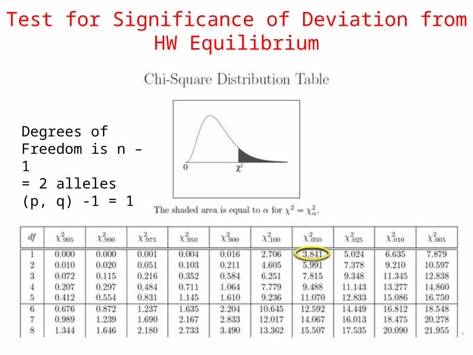
Test for Significance of Deviation from HW Equilibrium

Degrees of Freedom is n – 1 = 2 alleles (p, q) -1 = 1

Evolutionary Mechanisms

Genetic Drift (and Inbreeding)

DEVIATION from

Hardy-Weinberg EquilibriumIndicates that

EVOLUTIONIs happening

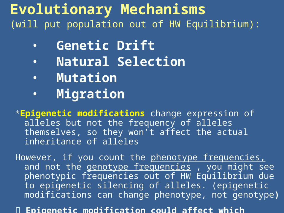
Evolutionary Mechanisms (will put population out of HW Equilibrium):

• Genetic Drift• Natural Selection• Mutation• Migration

*Epigenetic modifications change expression of alleles but not the frequency of alleles themselves, so they won’t affect the actual inheritance of alleles

However, if you count the phenotype frequencies, and not the genotype frequencies , you might see phenotypic frequencies out of HW Equilibrium due to epigenetic silencing of alleles. (epigenetic modifications can change phenotype, not genotype)

Epigenetic modification could affect which alleles are exposed to natural selection (no effect of Genetic Drift)

Natural Selection

Without genetic or epigenetic variation, Natural

Selection cannot occur

Mutation generates genetic variation

Epigenetic modification changes expression of

genes

Genetic Drift causes fluctuations in allele frequencies and can

reduce genetic variation

Sources of Genetic Variation

Natural Selection acts on genetic or epigenetic

variation in a population

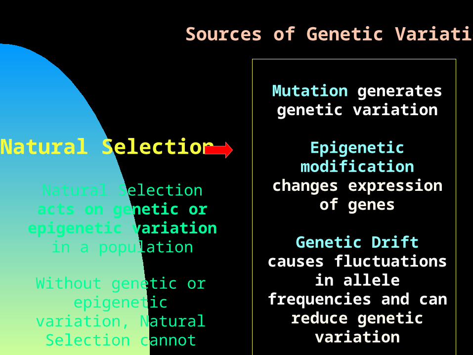
Natural Selection

Without genetic or epigenetic variation, Natural

Selection cannot occur

Mutation generates genetic variation

Epigenetic modification changes expression of

genes

Genetic Drift causes fluctuations in allele frequencies and can

reduce genetic variation

Sources of Genetic Variation

Natural Selection acts on genetic or epigenetic

variation in a population

(1) Migration

(2) Genetic Drift

(3) Effective Population Size

(4) Model of Genetic Drift

(5) Heterozygosity

(6) A Consequence of Genetic Drift: Inbreeding

Today’s OUTLINE:

Migration (fairly obvious)

Can act as a Homogenizing force

(If two populations are different, migration between them can reduce the differences)

A population could go out of HW equilibrium with a lot of migration

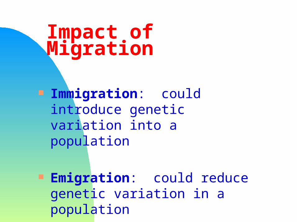
Impact of Migration

Immigration: could introduce genetic variation into a population

Emigration: could reduce genetic variation in a population

Random Genetic Drift

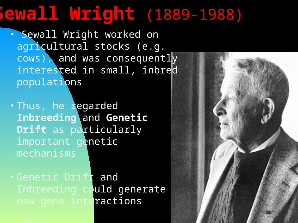
• Sewall Wright worked on agricultural stocks (e.g. cows), and was consequently interested in small, inbred populations

• Thus, he regarded Inbreeding and Genetic Drift as particularly important genetic mechanisms

• Genetic Drift and Inbreeding could generate new gene interactions

• These new gene interactions (epistasis caused by new recombinations) are the main substrate for selection

Sewall Wright (1889-1988)

“Null Model” No Evolution: Null Model to test if no evolution

is happening should simply be a population in Hardy-Weinberg Equilibrium

No Selection: Null Model to test whether Natural Selection is occurring should have no selection, but should include Genetic Drift This is because Genetic Drift is operating even

when there is no Natural Selection

“Null Model” No Selection: A model that tests for the

presence of Natural Selection should include Genetic Drift

This is because Genetic Drift is operating even when there is no Natural Selection

So the null model that tests for natural selection should include demography, population growth and decline, as population size directly affects the level of genetic drift acting on a population

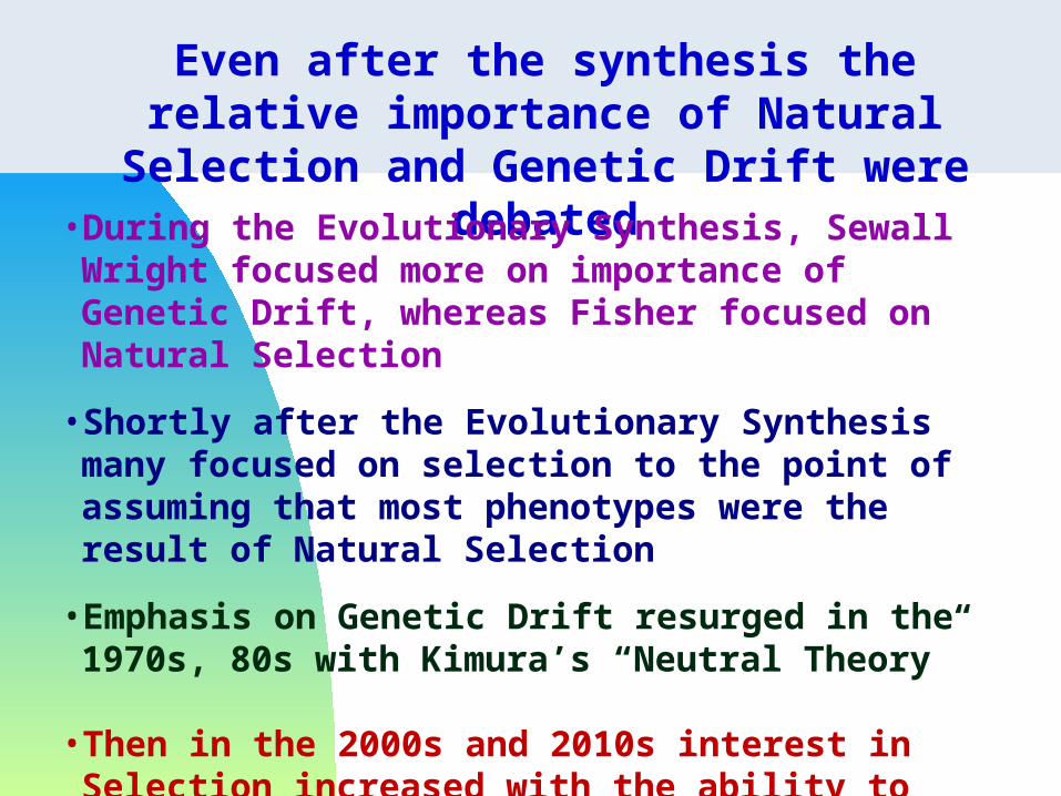
Even after the synthesis the relative importance of Natural Selection and Genetic Drift were debated

• During the Evolutionary Synthesis, Sewall Wright focused more on importance of Genetic Drift, whereas Fisher focused on Natural Selection

• Shortly after the Evolutionary Synthesis many focused on selection to the point of assuming that most phenotypes were the result of Natural Selection

• Emphasis on Genetic Drift resurged in the 1970s, 80s with Kimura’s “Neutral Theory”

• Then in the 2000s and 2010s interest in Selection increased with the ability to detect signatures of Natural Selection in genome sequence data

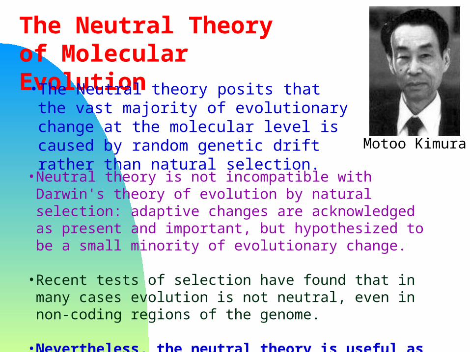
Motoo Kimura (1924-1994)

The Neutral Theory of Molecular Evolution

Classic Paper: Kimura, Motoo. 1968. Evolutionary rate at the molecular level. Nature. 217: 624–626.

Classic Book: Kimura, Motoo (1983). The neutral theory of molecular evolution. Cambridge University Press.

Molecular Clock

Figure: the rate of evolution of hemoglobin. Each point on the graph is for a pair of species, or groups of species. From Kimura (1983).

Observations of amino acid changes that occurred during the divergence between species, show that molecular evolution (mutations) takes place at a roughly constant rate.

This suggests that molecular evolution is constant enough to provide a “molecular clock” of evolution, and that the amount of molecular change between two species measures how long ago they shared a common ancestor.

From this, Kimura concluded that not much selection is going on (because the pattern of regular mutations is not obscured by selection), and that most evolution is influenced by Genetic Drift.

The Neutral Theory of Molecular Evolution

• Neutral theory is not incompatible with Darwin's theory of evolution by natural selection: adaptive changes are acknowledged as present and important, but hypothesized to be a small minority of evolutionary change.

• Recent tests of selection have found that in many cases evolution is not neutral, even in non-coding regions of the genome.

• Nevertheless, the neutral theory is useful as the null hypothesis, for testing whether natural selection is occurring.

Motoo Kimura

• The Neutral theory posits that the vast majority of evolutionary change at the molecular level is caused by random genetic drift rather than natural selection.

I. Random Genetic Drift

Definition: Changes in allele frequency from one generation to the next simply due to chance (sampling error).

This is a NON ADAPTATIVE evolutionary force.

Darwin did not consider genetic drift as an evolutionary force, only natural selection.

Genetic Drift

Genetic Drift happens when populations are limited in size, violating HW assumption of infinite population size

When population is large, chance events cancel each other out

When population is small, random differences in reproductive success begin to matter much more

Effective Population Size

In Evolution, when we talk about population size, we mean effective population size

Effective Population Size

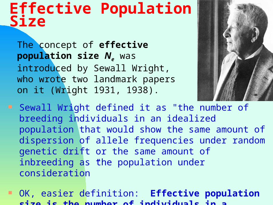
Sewall Wright defined it as "the number of breeding individuals in an idealized population that would show the same amount of dispersion of allele frequencies under random genetic drift or the same amount of inbreeding as the population under consideration”

OK, easier definition: Effective population size is the number of individuals in a population that actually contribute offspring to the next generation.

The concept of effective population size Ne was introduced by Sewall Wright, who wrote two landmark papers on it (Wright 1931, 1938).

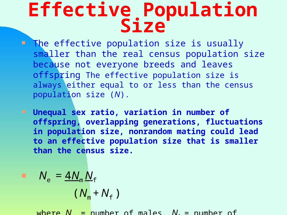
Effective Population Size The effective population size is usually smaller than the real

census population size because not everyone breeds and leaves offspring The effective population size is always either equal to or less than the census population size (N).

Unequal sex ratio, variation in number of offspring, overlapping generations, fluctuations in population size, nonrandom mating could lead to an effective population size that is smaller than the census size.

Ne = 4Nm Nf

(Nm + Nf )

where Nm = number of males, Nf = number of females

from this equation, you can see that unequal sex ratio would lead to lower Ne

Why do we care about effective population size Ne?

Because Ne is the actual unit of evolution, rather than the census size N

Why? Because only the alleles that actually get passed onto the next generation count in terms of evolution… the individuals that do not mate or have offspring are evolutionary dead ends…

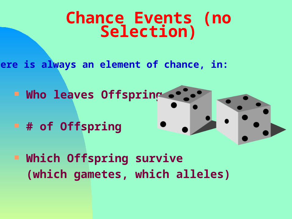
Chance Events (no Selection)

Who leaves Offspring

# of Offspring

Which Offspring survive

(which gametes, which alleles)

There is always an element of chance, in:

Example of sampling errorGreen fur: G (dominant)Blue fur: b (recessive)

If Gb x Gb mate, the next generation is expected to have: 3:1 Ratio of Green to blue (GG, Gb, bG, bb)

But this might not happen

One family could get this unusual frequency just due to chance: You might get: bb, bb, bb, bbAnd, so you might accidentally lose the G allele not for any reason, but just due to chance

The larger the population, the more these effects average out, and frequencies approach HW equilibrium

Why is this not Selection?

Selection happens when some survive for a reason: better adapted.

Genetic Drift is just a numbers game. Which gamete gets fertilized, which allele gets passed on is RANDOM

Consequences of Genetic Drift

Random fluctuations in allele frequency

If population size is reduced:

1. At the Allelic level: Random fixation of Alleles (loss of alleles)

2. At the Genotypic level: Loss of Heterozygosity (because of fewer alleles)

Random Shift in Allele Frequencies across Generations

Probability of loss of alleles is greater in smaller populations

For example, if there are 50 different alleles in population

…and a new population is founded by only 10 individuals

Then the new population will be unable to capture all 50 alleles, and many of the alleles will be lost

Bottleneck Effect

Random fixation of alleles

FIXATION: When an allele frequency becomes 100%

The other alleles are lost by chance

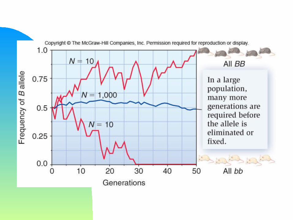
Fluctuations are much larger in smaller populations

Probability of fixation of an allele

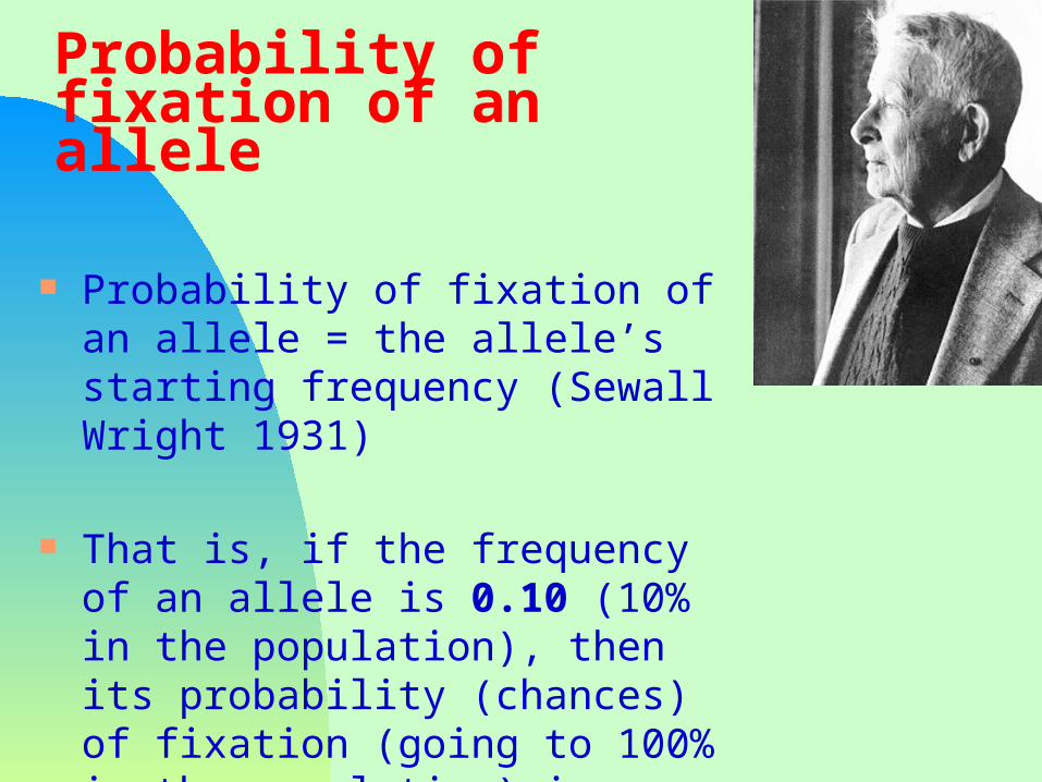
Probability of fixation of an allele = the allele’s starting frequency (Sewall Wright 1931)

That is, if the frequency of an allele is 0.10 (10% in the population), then its probability (chances) of fixation (going to 100% in the population) is 0.10, or 10%

Probability of fixation of an allele

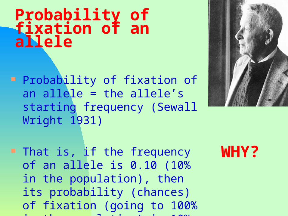
Probability of fixation of an allele = the allele’s starting frequency (Sewall Wright 1931)

That is, if the frequency of an allele is 0.10 (10% in the population), then its probability (chances) of fixation (going to 100% in the population) is 10%

WHY?

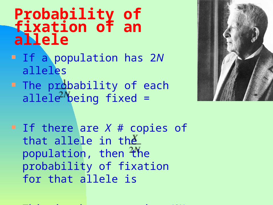
Probability of fixation of an allele If a population has 2N alleles The probability of each allele being

fixed =

If there are X # copies of that allele in the population, then the probability of fixation for that allele is

This is the proportion (%) of alleles in the population

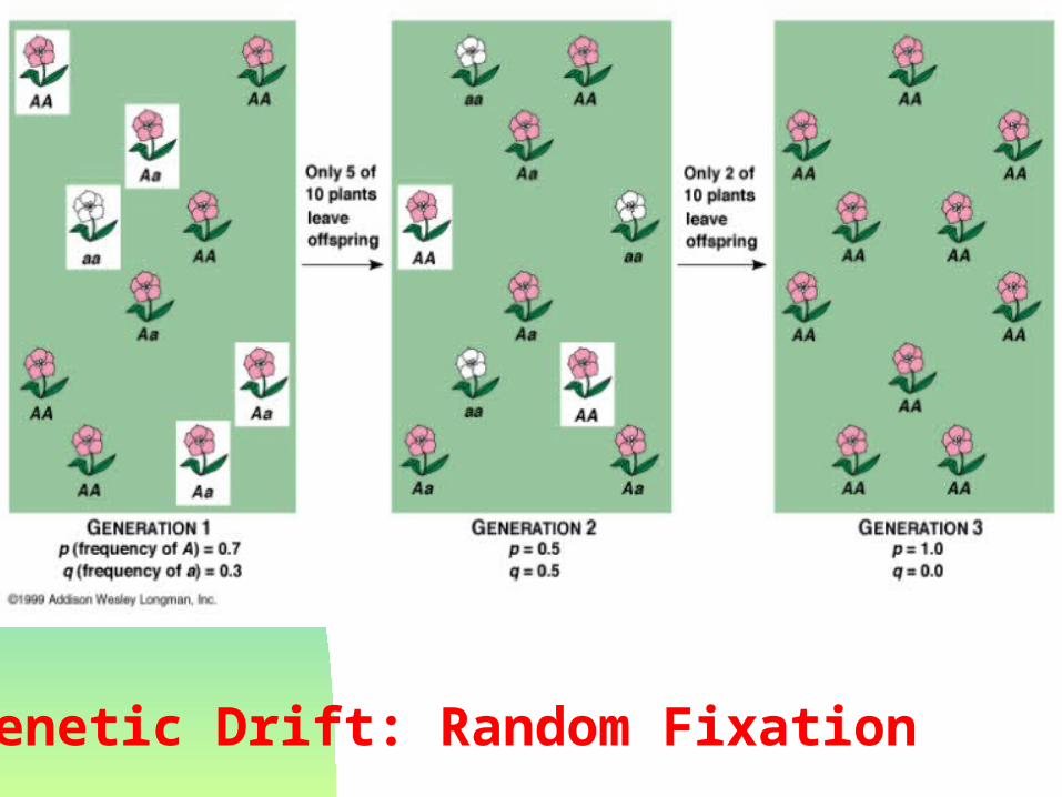
Genetic Drift: Random Fixation

After 7 generations, all allelic diversity was lost… the population became fixed for allele #1 just due to chance

Genetic Drift: Random Fixation

As populations get smaller, the probability of fixation goes up

Genetic Drift: Random Fixation

Heterozygosity Heterozygosity: frequency of heterozygotes in

a population (% of heterozygotes)

Often used as an estimate of genetic variation in a population

HW expected frequency of heterozygotes in a population = 2p(1-p)

As genetic drift drives alleles toward fixation or loss, the reduction in number of alleles causes the frequency of heterozygotes to go down

HeterozygosityThe Expected Heterozygosity following a population bottleneck

(frequency of Heterozygotes in the next generation = Hg+1):

g+1 g

e

Note in this equation that as population size 2Ne gets small, heterozygosity in the next generation Hg+1, goes down

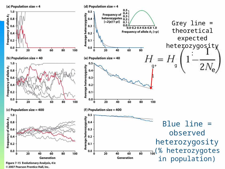
g+1 g

Grey line = theoretical expected

heterozygosity:

Blue line = observed heterozygosity (%

heterozygotes in population)

e

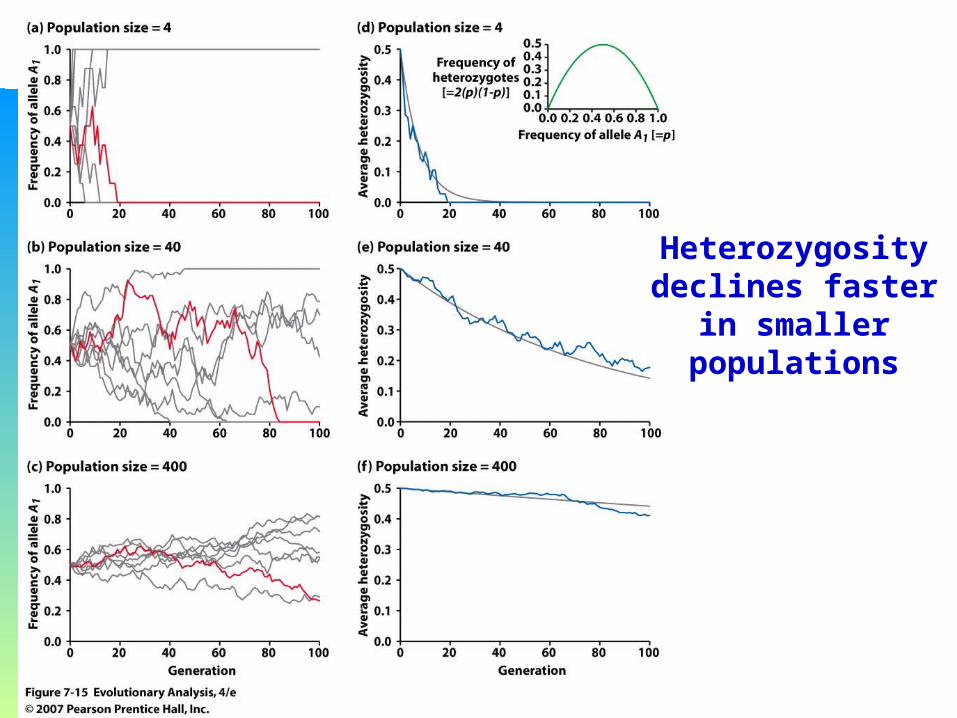
Heterozygosity declines faster in

smaller populations

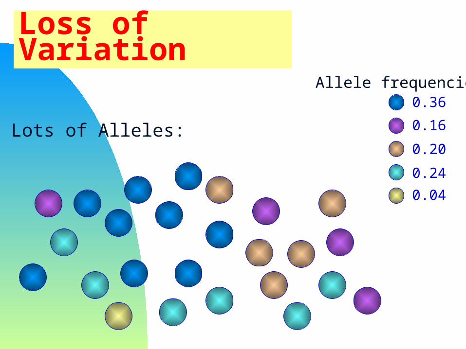
Loss of Variation

0.36

0.16

0.20

0.24

0.04

Allele frequencies

Lots of Alleles:

Possible genotype combinations

Lots of alleles --> Lots of genotypes:

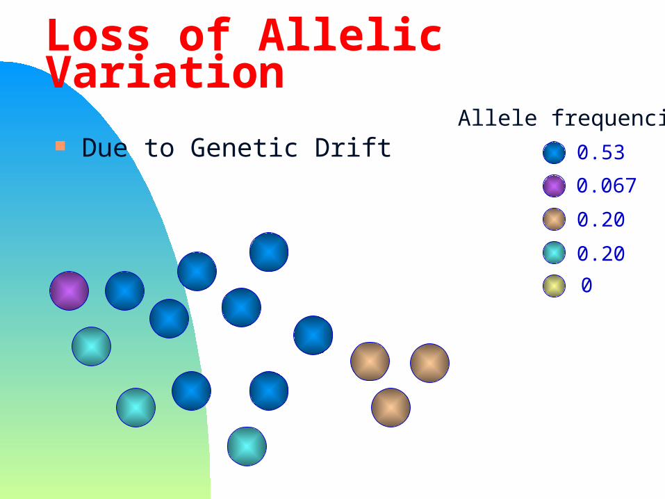
Loss of Allelic Variation

Due to Genetic Drift 0.53

0.067

0.20

0.20

0

Allele frequencies

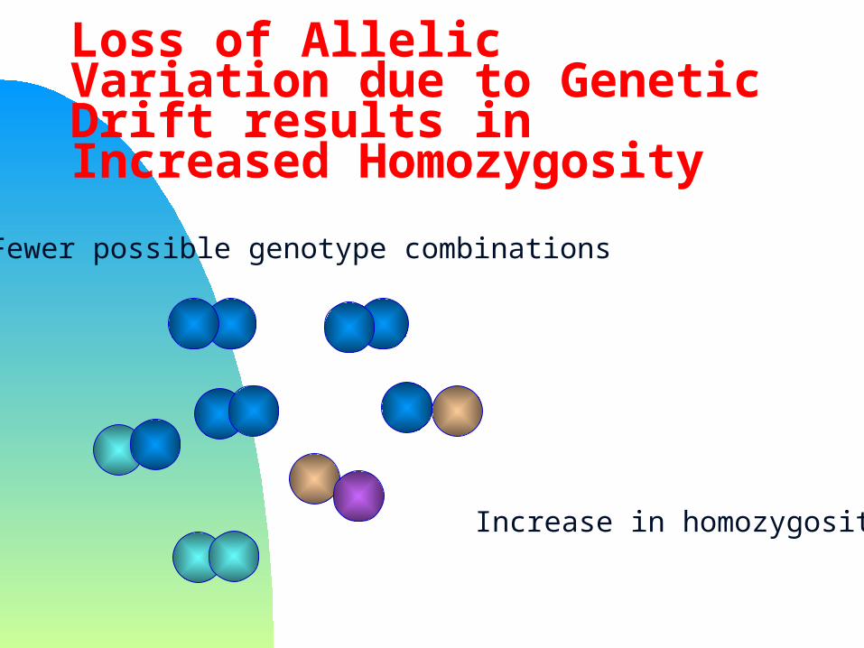
Loss of Allelic Variation due to Genetic Drift results in Increased Homozygosity

Increase in homozygosity

Fewer possible genotype combinations

No Genetic Variation = No Natural Selection

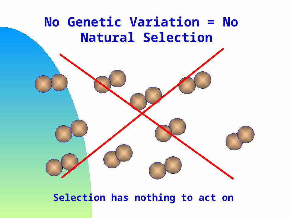
No Genetic Variation = No Natural Selection

Selection has nothing to act on

Genetic Drift and Natural Selection

Because of the randomness introduced by Genetic Drift, Natural Selection is less efficient when there is genetic drift

Thus, Natural Selection is more efficient in larger populations, and less effective in smaller populations

Allele A1 Demo

• Impact of Effective Population Size

• Impact of starting allele frequency

• Interaction between Natural Selection and Genetic Drift

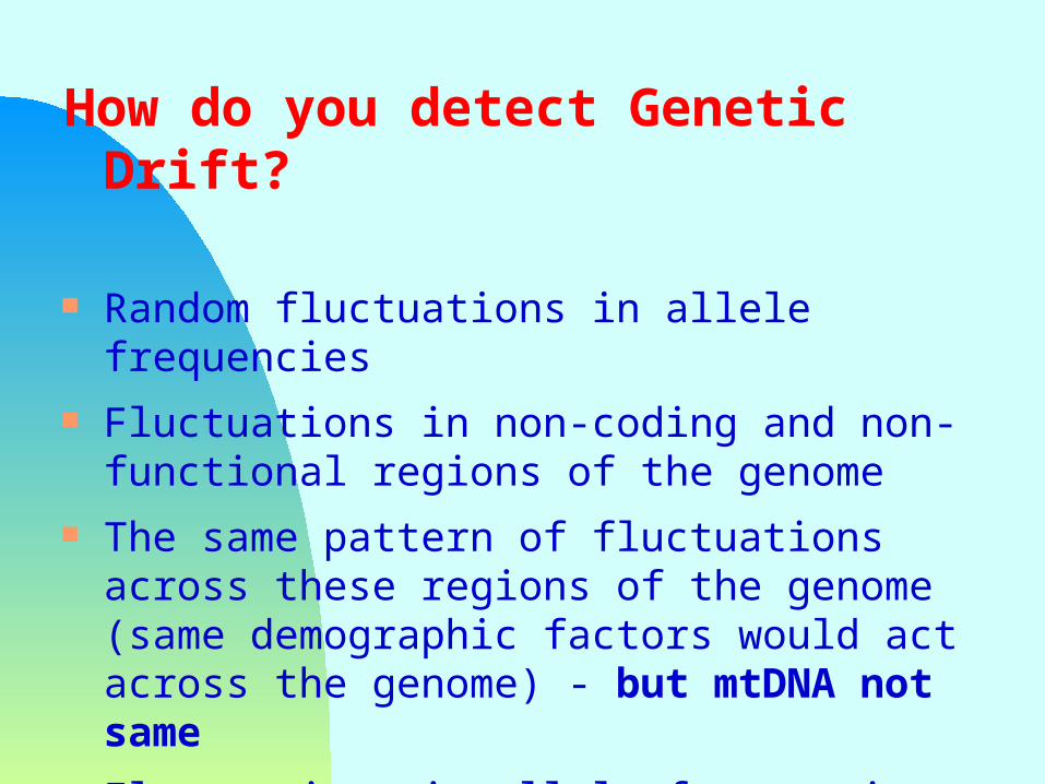
How do you detect Genetic Drift?

Random fluctuations in allele frequencies Fluctuations in non-coding and non-functional

regions of the genome The same pattern of fluctuations across these

regions of the genome (same demographic factors would act across the genome) - but mtDNA not same

Fluctuations in allele frequencies correspond to demography of the population (population size)

Consequences of Genetic Drift

---> Random fluctutations in allele frequency

If population size is reduced and Drift acts more intensely, we get:

1. At the Allelic level: Random fixation of Alleles (loss of alleles)

2. At the Genotypic level: Inbreeding, Reduction in Heterozygosity (because of fewer alleles)

Dilemma for Conservationists

• It is easier to remove genetic diversity than create it… especially variation that is potentially adaptive

Census size: Roughly 2000-3000 cheetahs live in Namibia today

The effective population size is much lower

2. Genetic Drift often leads to Inbreeding

Inbreeding is a consequence of Genetic drift in small populations, resulting from loss of alleles

Due to loss of alleles, there is an increase in homozygosity

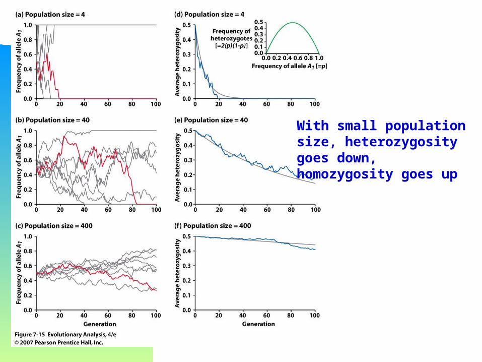
With small population size, heterozygosity goes down, homozygosity goes up

Inbreeding

Mating among genetic relatives, often because of small population size

Alleles at a locus will more likely become homozygous

A consequence of loss of alleles due to genetic drift (reduction in population size)

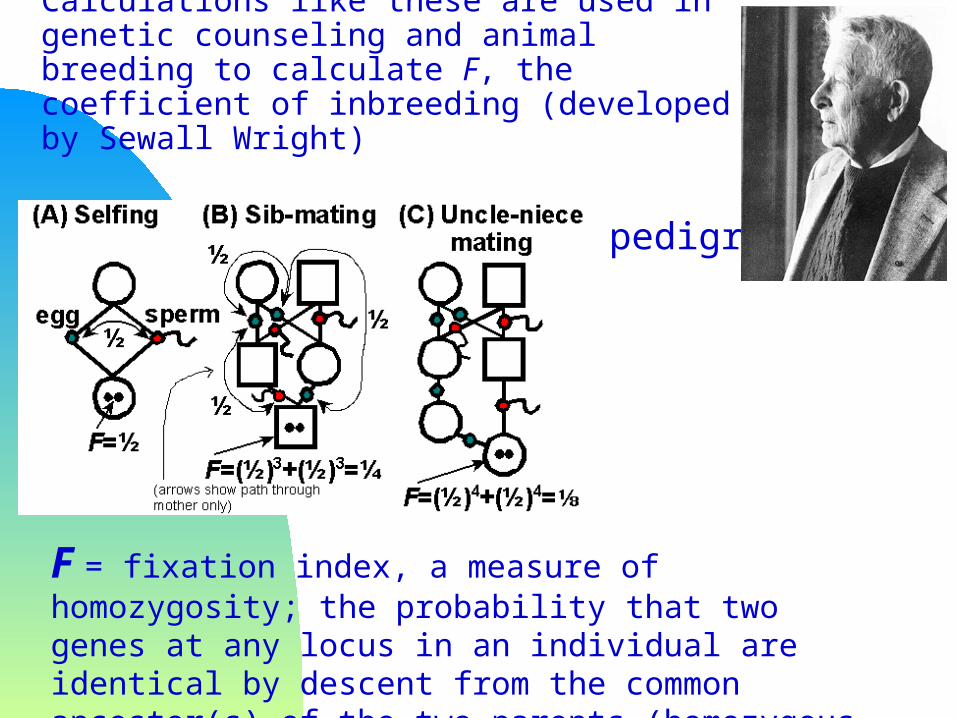
Calculations like these are used in genetic counseling and animal breeding to calculate F, the coefficient of inbreeding (developed by Sewall Wright)

Show popgen pedigree

F = fixation index, a measure of homozygosity; the probability that two genes at any locus in an individual are identical by descent from the common ancestor(s) of the two parents (homozygous, rather than heterozygous).

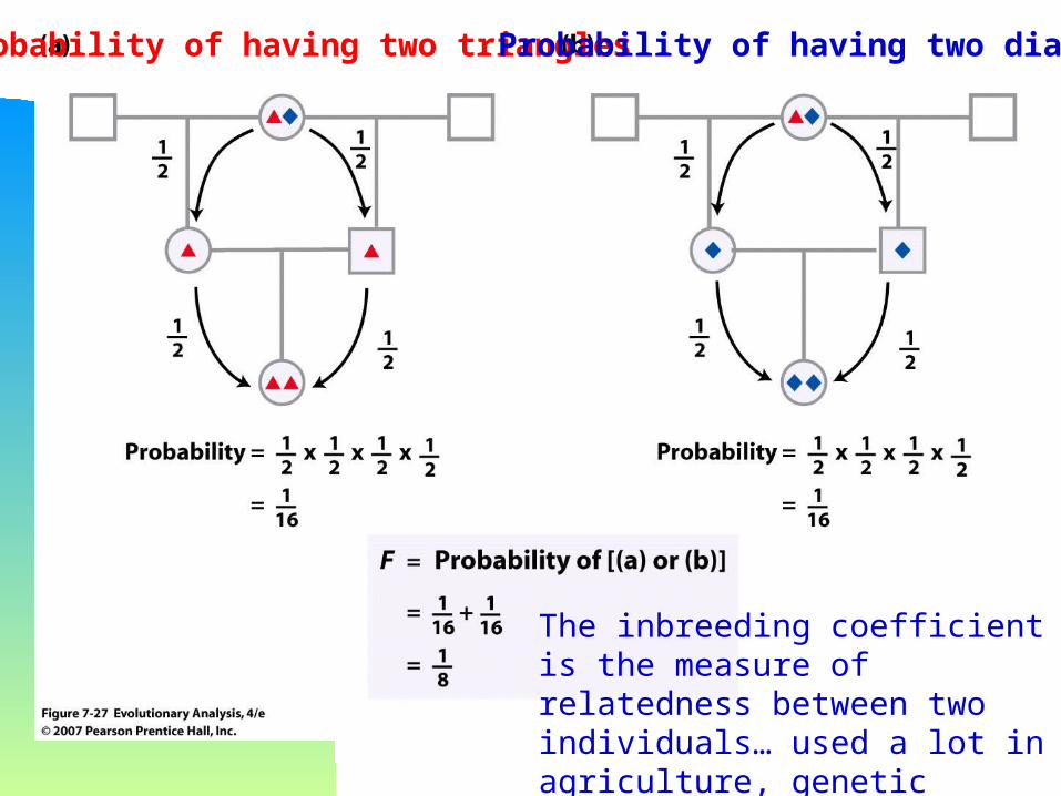
The inbreeding coefficient is the measure of relatedness between two individuals… used a lot in agriculture, genetic counseling, etc.

Probability of having two triangles Probability of having two diamonds

small population size genetic drift loss of alleles decrease in heterozygosity increase in

homozygosity

increase of exposure of deleterious alleles

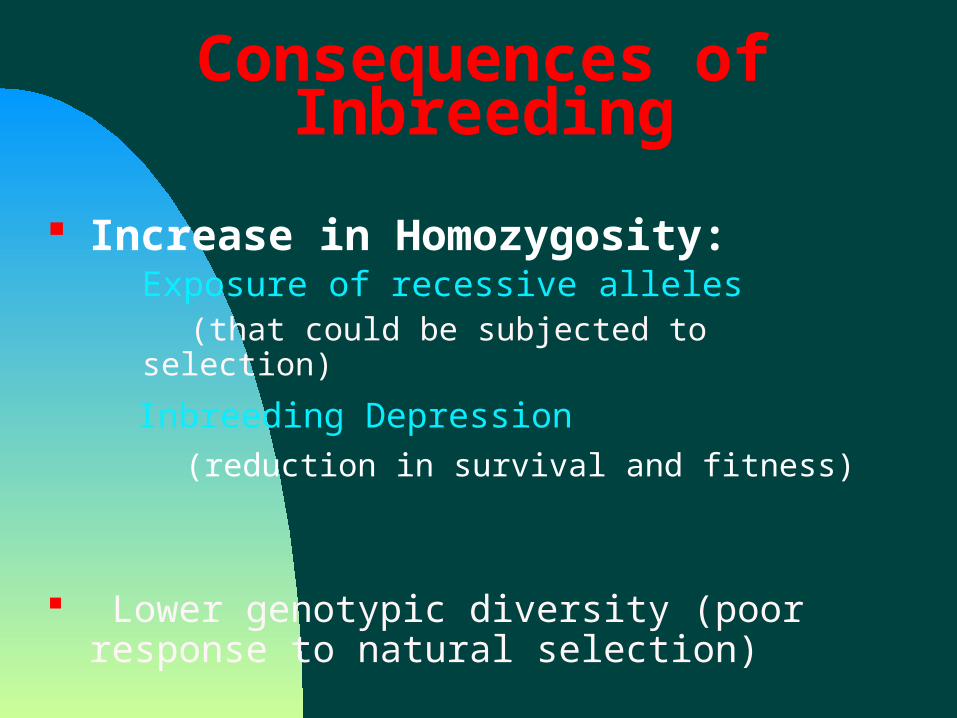
Consequences of Inbreeding

Increase in Homozygosity:Exposure of recessive alleles (that could be subjected to selection)

Inbreeding Depression (reduction in survival and fitness)

Lower genotypic diversity (poor response to natural selection)

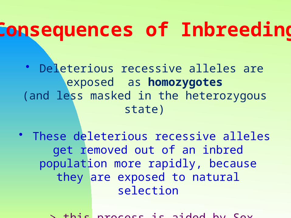
Consequences of Inbreeding

• Deleterious recessive alleles are exposed as homozygotes

(and less masked in the heterozygous state)

• These deleterious recessive alleles get removed out of an inbred population more rapidly, because they

are exposed to natural selection

---> this process is aided by Sex, discussed in Next Lecture (on Variation)

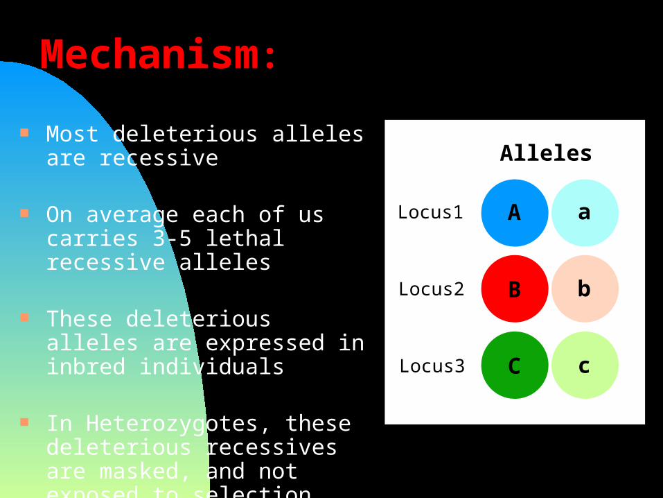
Mechanism:

Most deleterious alleles are recessive

On average each of us carries 3-5 lethal recessive alleles

These deleterious alleles are expressed in inbred individuals

In Heterozygotes, these deleterious recessives are masked, and not exposed to selection

Alleles

A a

B b

C c

Locus1

Locus2

Locus3

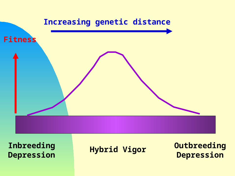
InbreedingDepression

Hybrid Vigor OutbreedingDepression

Increasing genetic distance

Fitness

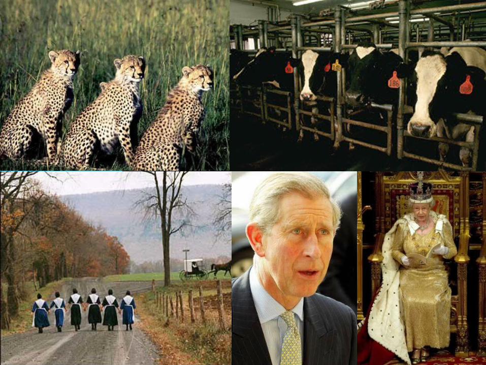
Examples of Inbreeding

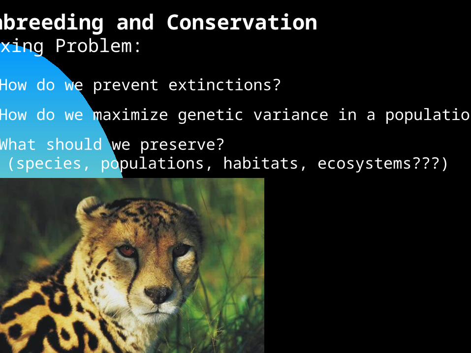
Inbreeding and ConservationVexing Problem:

How do we prevent extinctions?

How do we maximize genetic variance in a population?

What should we preserve? (species, populations, habitats, ecosystems???)

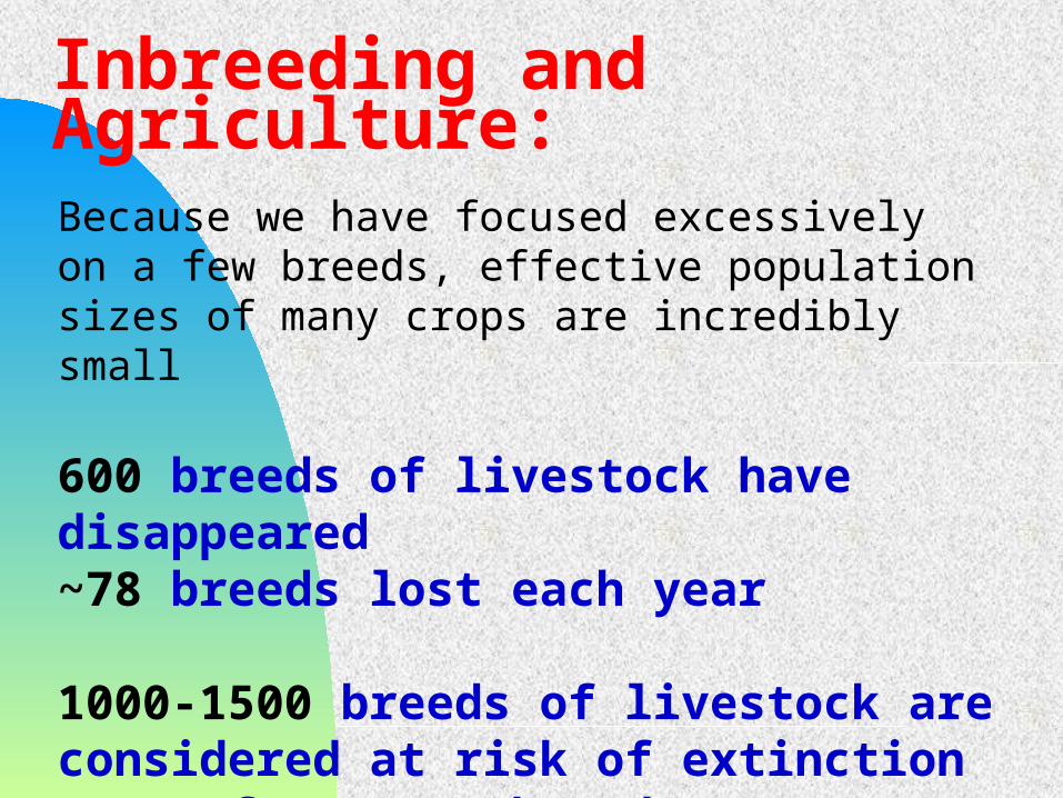
Inbreeding and Agriculture:

Because we have focused excessively on a few breeds, effective population sizes of many crops are incredibly small

600 breeds of livestock have disappeared~78 breeds lost each year

1000-1500 breeds of livestock are considered at risk of extinction(30% of current breeds)

8 million Holstein cows are descendents of 37 individuals!!!

Neurological disordersAutoimmune diseasesFertility problems

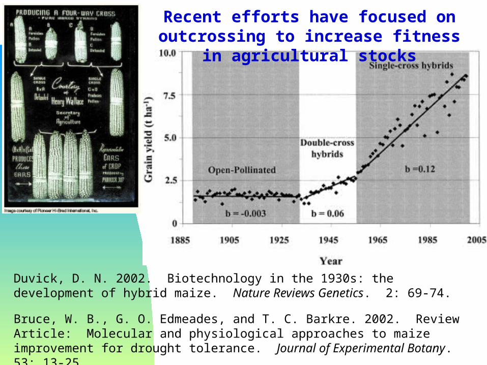
Duvick, D. N. 2002. Biotechnology in the 1930s: the development of hybrid maize. Nature Reviews Genetics. 2: 69-74.

Bruce, W. B., G. O. Edmeades, and T. C. Barkre. 2002. Review Article: Molecular and physiological approaches to maize improvement for drought tolerance. Journal of Experimental Botany. 53: 13-25.

Recent efforts have focused on outcrossing to increase fitness in agricultural stocks

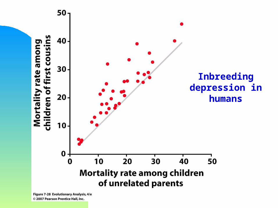
Inbreeding depression in

humans

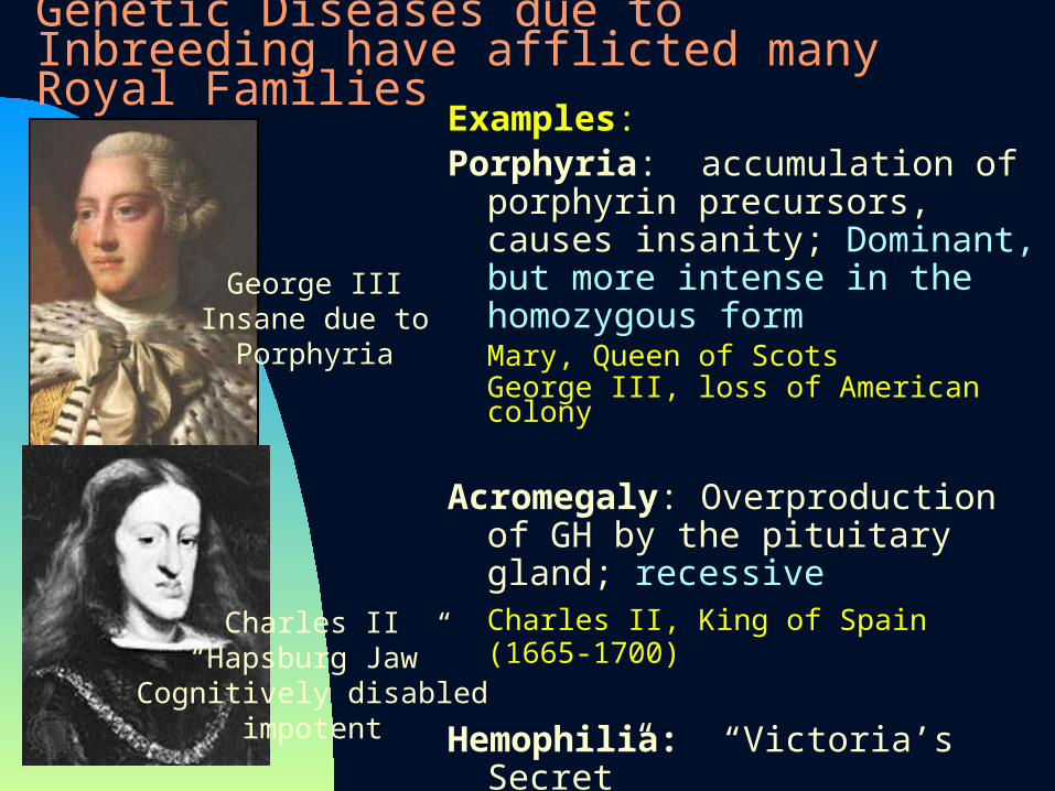
Genetic Diseases due to Inbreeding have afflicted many Royal Families

Examples: Porphyria: accumulation of porphyrin

precursors, causes insanity; Dominant, but more intense in the homozygous form Mary, Queen of ScotsGeorge III, loss of American colony

Acromegaly: Overproduction of GH by the pituitary gland; recessiveCharles II, King of Spain (1665-1700)

Hemophilia: “Victoria’s Secret”X-linked, shows up in malesDaughters spread it among the royals, downfall of Russian monarchy

George IIIInsane due to

Porphyria

Charles II“Hapsburg Jaw”

Cognitively disabledimpotent

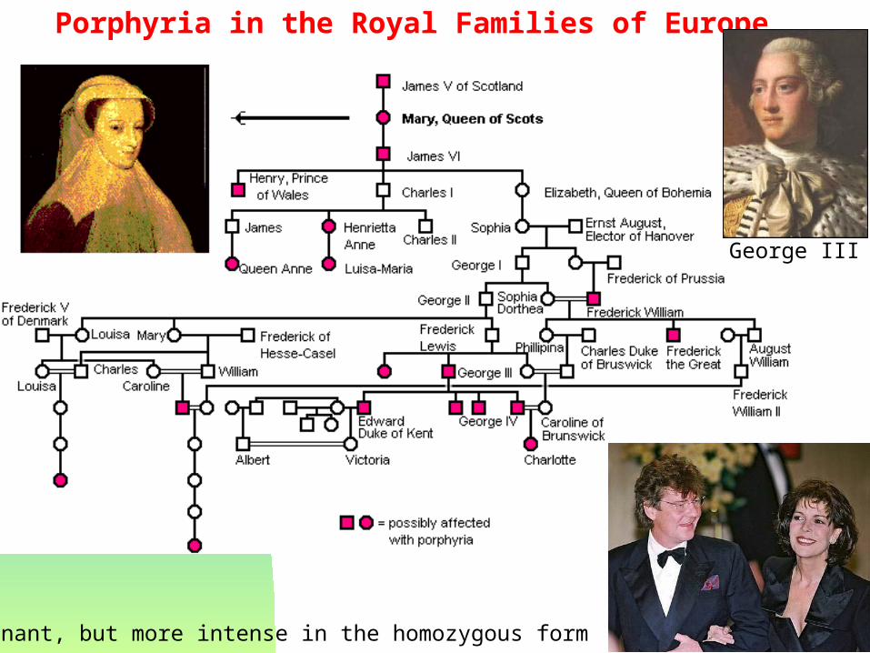
Porphyria in the Royal Families of Europe

Dominant, but more intense in the homozygous form

George III

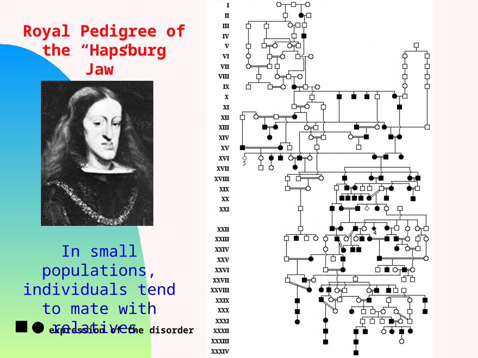
Royal Pedigree of the “Hapsburg Jaw”

= expression of the disorder

In small populations, individuals tend to mate

with relatives

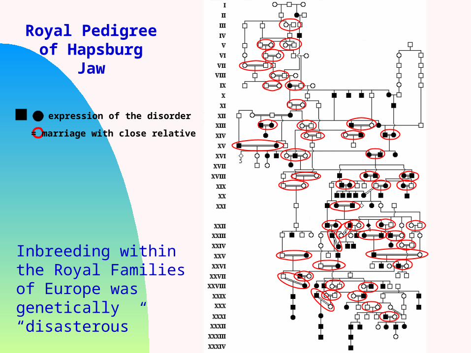
Royal Pedigree of Hapsburg Jaw

= marriage with close relative

Inbreeding within the Royal Families of Europe was genetically “disasterous”

= expression of the disorder

Inbreeding within Royal Families has been reduced

in recent years

Diana was a 7th cousin of Charles, rather than a first or second

cousin (which was the normal practice previously)

Kate Middleton is neither an aristocrat nor a royal, but the marriage was approved given the modern recognition of the perils of inbreeding… this marriage is an example of genetic immigration (Migration) into an enclosed population

Articles on British Royalty and Inbreeding:

News Article:http://www.telegraph.co.uk/news/worldnews/europe/spain/5158513/Inbreeding-caused-demise-of-the-Spanish-Habsburg-dynasty-new-study-reveals.html

Original Scientific Article:http://www.plosone.org/article/info:doi/10.1371/journal.pone.0005174

Descendents of ~200 Swiss who emigrated mid-1700s.

Amish in Lancaster County, PA

Closed genetic population for 12+ generations.

Host to 50+ identified inherited disorders(many more uncharacterized)

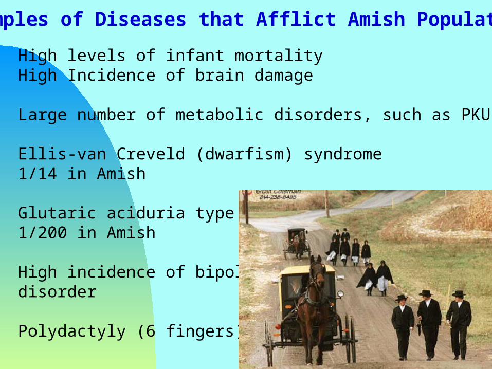
High levels of infant mortalityHigh Incidence of brain damage

Large number of metabolic disorders, such as PKU

Ellis-van Creveld (dwarfism) syndrome 1/14 in Amish

Glutaric aciduria type I1/200 in Amish

High incidence of bipolar disorder

Polydactyly (6 fingers)

Examples of Diseases that Afflict Amish Populations

There is nothing special about the Amish, genetically speaking (or Royal Families).

• There are about ~200 of you here, similar to the size of the founding Amish population in Lancaster county, Pennsylvania.

• If all of you were stranded on a desert island, eventually your descendents would be related and mating with one another.

• Each of us carries 3-5 lethal recessive alleles.

• If 200 people each had 3-5 different recessive lethals and started forming a closed population, eventually, hundreds of genetic disorders would emerge.

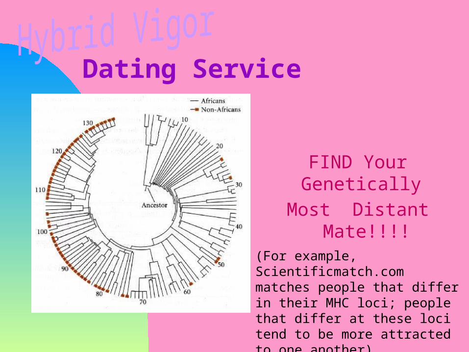
FIND Your Genetically

Most Distant Mate!!!!

Dating Service

(For example, Scientificmatch.com matches people that differ in their MHC loci; people that differ at these loci tend to be more attracted to one another)

Summary

(1) Genetic Drift occurs when a population is small, and leads to random loss of alleles due to sampling error

(2) Inbreeding, an extreme consequence of Genetic Drift, results in increases in homozygosity at many loci, including recessive lethals

CONCEPTS

Genetic Drift

Effective population size

Fixation

Heterozygosity

Inbreeding

Inbreeding Depression

Heterozygote advantage

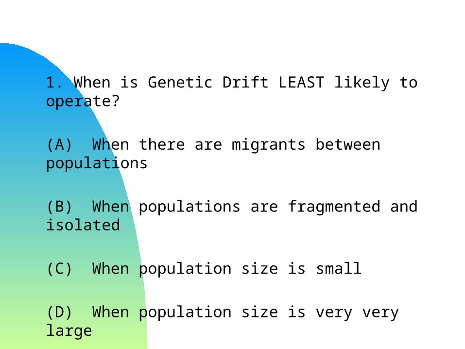
1. When is Genetic Drift LEAST likely to operate?

(A) When there are migrants between populations

(B) When populations are fragmented and isolated

(C) When population size is small

(D) When population size is very very large

2. Which of the following is FALSE regarding inbreeding?

(A) Inbreeding could result as a consequence after genetic drift has acted on a population

(B) Populations with lower allelic diversity tend to have lower genotypic diversity (more homozygous)

(C) Selection acts more slowly in inbred populations to remove deleterious recessive alleles

(D) One way to reduce inbreeding in a population is to bring in migrants from another population

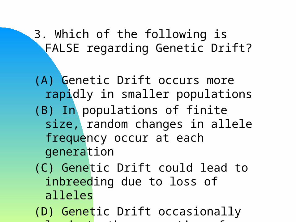
3. Which of the following is FALSE regarding Genetic Drift?

(A) Genetic Drift occurs more rapidly in smaller populations

(B) In populations of finite size, random changes in allele frequency occur at each generation

(C) Genetic Drift could lead to inbreeding due to loss of alleles

(D) Genetic Drift occasionally leads to the generation of favorable alleles

Answers to sample exam questions:

1D 2C 3D