Example problem: The Young Laplace equation - oomph-lib

Chapter 1

Example problem: The Young Laplace equation

This document discusses the finite-element-based solution of the Young Laplace equation, a nonlinearPDE that determines the static equilibrium shapes of droplets or bubbles. We start by reviewing the relevant theoryand then present the solution of a simple model problem.

Acknowledgement:

This tutorial and the associated driver codes were developed jointly with Cedric Ody (Ecole Polytechnique, Paris;now Rennes).

1.1 Theory

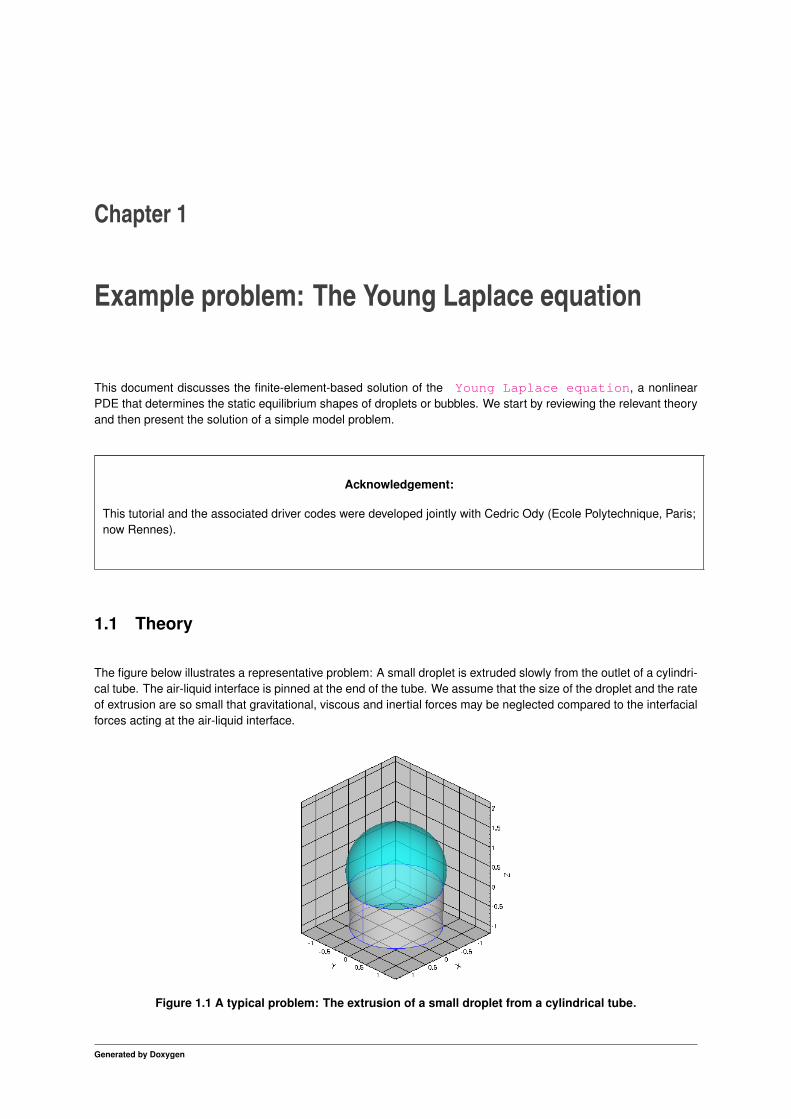
The figure below illustrates a representative problem: A small droplet is extruded slowly from the outlet of a cylindri-cal tube. The air-liquid interface is pinned at the end of the tube. We assume that the size of the droplet and the rateof extrusion are so small that gravitational, viscous and inertial forces may be neglected compared to the interfacialforces acting at the air-liquid interface.

Figure 1.1 A typical problem: The extrusion of a small droplet from a cylindrical tube.

Generated by Doxygen

2 Example problem: The Young Laplace equation

The shape of the air-liquid interface (the meniscus) is then determined by Laplace's law which expresses the balancebetween the (spatially constant) pressure drop across the meniscus, ∆p∗, and the surface tension forces acting atthe air-liquid interface,

∆p∗ = σκ∗,

where κ∗ is the mean curvature and σ the surface tension.

Non-dimensionalising all lengths on some problem-specific lengthscale L (e.g. the radius of the cylindrical tube)and scaling the pressure on the associated capillary scale, ∆p∗ = σ/L∆p, yields the non-dimensional form of theYoung-Laplace equation

∆p = κ.

This must be augmented by suitable boundary conditions, to be applied at the contact line – the line along whichthe meniscus meets the solid surface. We can either "pin" the position of the contact line (as in the above example),or prescribe thecontact angle at which the air-liquid interface meets the solid surface.

The mathematical problem may be interpreted as follows: Given the prescribed pressure drop ∆p (and thus κ), wewish to determine an interface shape of the required mean curvature κ that satisfies the boundary conditions alongthe contact line.

1.1.1 Cartesian PDE-based formulation

Expressing the (non-dimensional) height of the interface above the (x1, x2)-plane as x3 = u(x1, x2) yields thecartesian form of the Young-Laplace equation:

∆p = κ = −∇ · ∇u√1 + |∇u|2

,

where∇ = (∂/∂x1, ∂/∂x2)T Given the imposed pressure drop across the interface, this equation must be solvedfor u(x1, x2). Note that this is only possible if the interface can be projected onto the (x1, x2)-plane.

1.1.2 The principle of virtual displacements

The interface shape can also be determined from the principle of virtual displacements

δ

(∫S

ds

)=

∫S

∆pN · δN ds+

∮L

Tn · δR d l (1)

which may be derived from energetic considerations. Here the symbol δ denotes a variation, R is the positionvector to the interface, and the vector N is the unit normal to the meniscus. The left hand side of this equationrepresents the variation of the interfacial energy during a virtual displacement, and ds is an infinitesimal elementof the meniscus surface, S. The terms on the right hand side represent the virtual work done by the pressure andthe virtual work done by the surface tension forces acting at the free contact line, respectively. dl is the length ofan element of the contact line L, and Tn is the vector tangent to the interface and normal to the contact line. Notethat, if the contact line is pinned, the variation of its position is zero, δR = 0, and the line integral vanishes.

The variational formulation of the problem is particularly convenient for a finite-element-based solution; see, e.g. theSolid Mechanics Theory document for a discussion of how to discretise variational principles with finiteelements. The variational and PDE-based formulations are, of course, related to each other: The Young-Laplaceequation is the Euler-Lagrange equation of the variational principle.

Generated by Doxygen

1.1 Theory 3

1.1.3 Parametric representation

To deal with cases in which the interface cannot be projected onto the (x1, x2)-plane, we parametrise the meniscusby two intrinsic coordinates as R(ζ1, ζ2) ∈ R3, where (ζ1, ζ2) ∈ D ∈ R2. Furthermore, we parametrise thedomain boundary, ∂D, by a scalar coordinate ξ so that,

∂D =

{(ζ1, ζ2)

∣∣∣∣ (ζ1, ζ2) =(ζ[∂D]1 (ξ), ζ

[∂D]2 (ξ)

)}.

The normal to the meniscus is then given by

N =R,1 ×R,2

A1/2,

where the commas denote partial differentiation with respect to the intrinsic coordinates, and A1/2 = |R,1 ×R,2|is the square root of the surface metric tensor.

The area and length differentials required in variational principle are

ds = A1/2dζ1dζ2

and

dl =

∣∣∣∣∣∣dR(ζ[∂D]1 (ξ), ζ

[∂D]2 (ξ)

)dξ

∣∣∣∣∣∣ dξ,allowing us to write the principle of virtual displacements as

∫S

(δA1/2

A1/2− κN · δR

)A1/2dζ1dζ2 =

∮L

Tn · δR

∣∣∣∣∣∣dR(ζ[∂D]1 (ξ), ζ

[∂D]2 (ξ)

)dξ

∣∣∣∣∣∣ dξ.

1.1.4 The method of spines

In the current form, the variational principle cannot yield a unique solution because there are infinitely many vectorfields R(ζ1, ζ2) that parametrise the same interface shape. To remove this ambiguity, and to allow for interfaceshapes that cannot be projected onto the (x1, x2)-plane, we employ the so-called "Method of Spines". This methodwas originally proposed by Kistler and Scriven for the computation of free surface flows. We decompose the vectorR into two parts by writing it as

R(ζ1, ζ2) = B(ζ1, ζ2) + u(ζ1, ζ2) S(ζ1, ζ2).

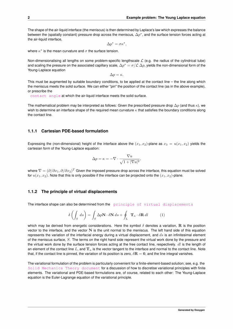
Here the "spine basis" B(ζ1, ζ2) and the "spines" S(ζ1, ζ2) are pre-determined vector fields that must be chosenby the user. Using this decomposition, the meniscus shape is determined by the scalar function u(ζ1, ζ2) whichrepresents the meniscus' displacement along the spines S.

The idea is illustrated in the simple 2D sketch below: the spine basis vectors, B(ζ), parametrise the straight linecorresponding to a flat meniscus. Positive values of u displace the meniscus along the spines, S(ζ) (the redvectors), whose orientation allows the representation of meniscus shapes that cannot be represented in cartesianform as x2 = u(x1).

Generated by Doxygen

4 Example problem: The Young Laplace equation

x1

x2

B(ζ)

S (ζ)

(ζ)

ζ

u

Figure 1.2 Sketch illustrating the parametrisation of the meniscus by the Method of Spines.

The spine basis and the spines themselves must be chosen such that the mapping from (ζ1, ζ2) to R(ζ1, ζ2) isone-to-one, at least for the meniscus shapes of interest. Pinned boundary conditions of the form R|∂D = Rpinned

are most easily imposed by choosing the spine basis such that B|∂D = Rpinned, implying that u|∂D = 0.

The simplest possible choice for the spines and spine basis is one that returns the problem to its original cartesianformulation. This is achieved by setting B(ζ1, ζ2) = (ζ1, ζ2, 0)T and S(ζ1, ζ2) = (0, 0, 1)T .

1.1.5 Displacement Control

The Young-Laplace equation is a highly nonlinear PDE. We therefore require a good initial guess for the solution inorder to ensure the convergence of the Newton iteration. In many cases good initial guesses can be provided by asimple, physically motivated continuation method. For instance in the model problem shown above, the computationwas started by computing the solution for ∆p = κ = 0 – a flat interface. This solution was then used as the initialguess for the solution at a small positive value of ∆p. This process was continued, allowing us to compute stronglydeformed meniscus shapes. This method works well, provided small increments in the control parameter ∆p (orequivalently, κ) create small changes in the interface shape. This is not always the case, however, as we shallsee in the example below. In such cases it is often possible to re-formulate the problem, using the displacementcontrol method discussed in the solid mechanics tutorials. Rather than prescribing the pressure drop∆p we prescribe the displacement of a control point on the meniscus and regard the pressure drop required toachieve this displacement as an unknown. Since the implementation of the method is very similar to that used forsolid mechanics problems, we shall not discuss it in detail here but refer to the appropriate solid mechanicstutorial.

1.2 An example problem: A barrel-shaped meniscus

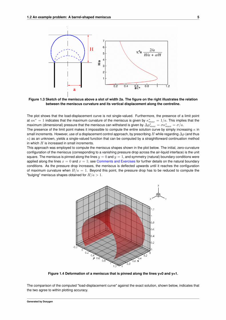
As an example, we consider the following problem: Fluid is extruded from an infinitely long, parallel-sided slot ofwidth 2a. If we assume that the air-liquid interface is pinned at the edges of the slot, as shown in the sketchbelow, the problem has an obvious exact solution. The air-liquid interface must have constant mean curvature, so,assuming that its shape does not vary along the slot, the meniscus must be a circular cylinder. If we characterise themeniscus' shape by its vertical displacement along the centreline, H , the (dimensional) curvature of the air-liquidinterface is given by

κ∗ =2/a

H/a+ a/H.

The plot of this function, shown in the right half of the figure below, may be interpreted as a "load-displacementdiagram" as it shows the deflection of the meniscus as a function of the imposed non-dimensional pressure dropacross the air-liquid interface, ∆p = aκ∗.

Generated by Doxygen

1.2 An example problem: A barrel-shaped meniscus 5

Figure 1.3 Sketch of the meniscus above a slot of width 2a. The figure on the right illustrates the relationbetween the meniscus curvature and its vertical displacement along the centreline.

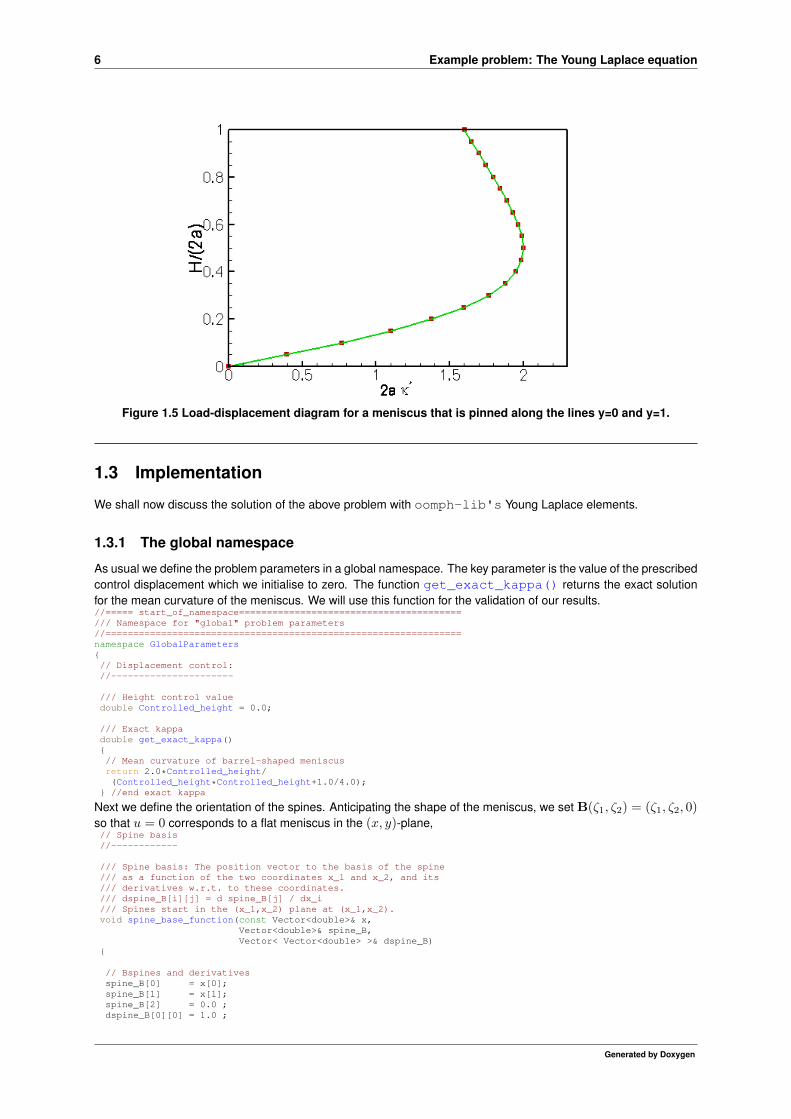
The plot shows that the load-displacement curve is not single-valued. Furthermore, the presence of a limit pointat aκ∗ = 1 indicates that the maximum curvature of the meniscus is given by κ∗max = 1/a. This implies that themaximum (dimensional) pressure that the meniscus can withstand is given by ∆p∗max = σκ∗max = σ/a.The presence of the limit point makes it impossible to compute the entire solution curve by simply increasing κ insmall increments. However, use of a displacement control approach, by prescribingH while regarding ∆p (and thusκ) as an unknown, yields a single-valued function that can be computed by a straightforward continuation methodin which H is increased in small increments.This approach was employed to compute the meniscus shapes shown in the plot below. The initial, zero-curvatureconfiguration of the meniscus (corresponding to a vanishing pressure drop across the air-liquid interface) is the unitsquare. The meniscus is pinned along the lines y = 0 and y = 1, and symmetry (natural) boundary conditions wereapplied along the lines x = 0 and x = 1; see Comments and Exercises for further details on the natural boundaryconditions. As the pressure drop increases, the meniscus is deflected upwards until it reaches the configurationof maximum curvature when H/a = 1. Beyond this point, the pressure drop has to be reduced to compute the"bulging" meniscus shapes obtained for H/a > 1.

Figure 1.4 Deformation of a meniscus that is pinned along the lines y=0 and y=1.

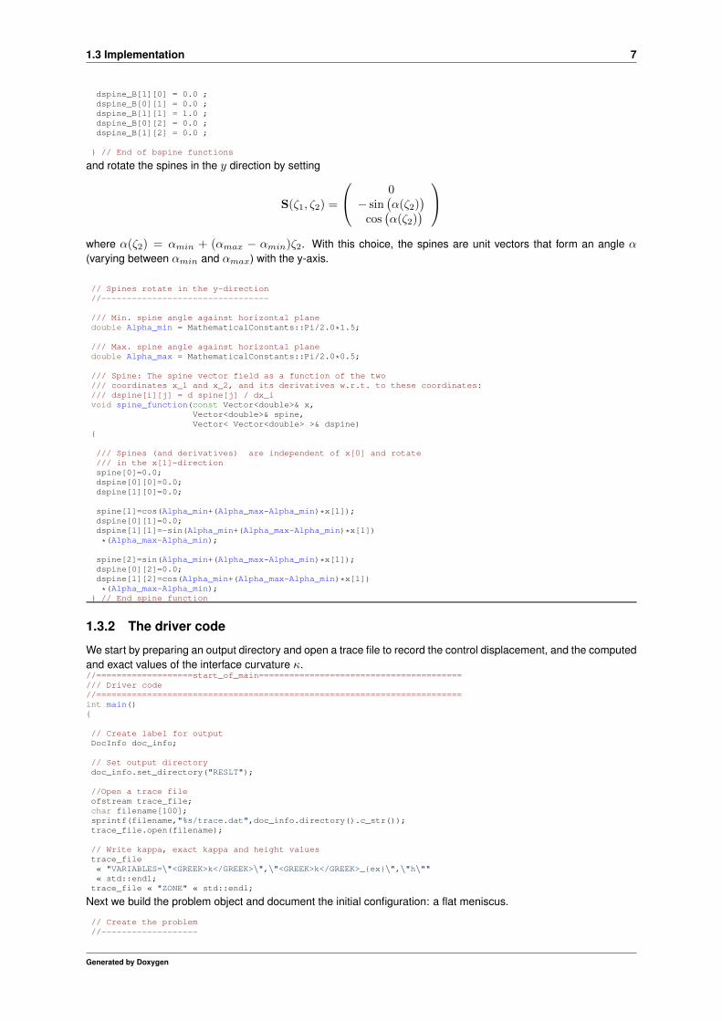
The comparison of the computed "load-displacement curve" against the exact solution, shown below, indicates thatthe two agree to within plotting accuracy.

Generated by Doxygen

6 Example problem: The Young Laplace equation

Figure 1.5 Load-displacement diagram for a meniscus that is pinned along the lines y=0 and y=1.

1.3 Implementation

We shall now discuss the solution of the above problem with oomph-lib's Young Laplace elements.

1.3.1 The global namespace

As usual we define the problem parameters in a global namespace. The key parameter is the value of the prescribedcontrol displacement which we initialise to zero. The function get_exact_kappa() returns the exact solutionfor the mean curvature of the meniscus. We will use this function for the validation of our results.//===== start_of_namespace========================================/// Namespace for "global" problem parameters//================================================================namespace GlobalParameters{// Displacement control://----------------------

/// Height control valuedouble Controlled_height = 0.0;

/// Exact kappadouble get_exact_kappa(){// Mean curvature of barrel-shaped meniscusreturn 2.0*Controlled_height/(Controlled_height*Controlled_height+1.0/4.0);

} //end exact kappa

Next we define the orientation of the spines. Anticipating the shape of the meniscus, we set B(ζ1, ζ2) = (ζ1, ζ2, 0)so that u = 0 corresponds to a flat meniscus in the (x, y)-plane,// Spine basis//------------

/// Spine basis: The position vector to the basis of the spine/// as a function of the two coordinates x_1 and x_2, and its/// derivatives w.r.t. to these coordinates./// dspine_B[i][j] = d spine_B[j] / dx_i/// Spines start in the (x_1,x_2) plane at (x_1,x_2).void spine_base_function(const Vector<double>& x,

Vector<double>& spine_B,Vector< Vector<double> >& dspine_B)

{

// Bspines and derivativesspine_B[0] = x[0];spine_B[1] = x[1];spine_B[2] = 0.0 ;dspine_B[0][0] = 1.0 ;

Generated by Doxygen

1.3 Implementation 7

dspine_B[1][0] = 0.0 ;dspine_B[0][1] = 0.0 ;dspine_B[1][1] = 1.0 ;dspine_B[0][2] = 0.0 ;dspine_B[1][2] = 0.0 ;

} // End of bspine functions

and rotate the spines in the y direction by setting

S(ζ1, ζ2) =

0− sin

(α(ζ2)

)cos(α(ζ2)

)

where α(ζ2) = αmin + (αmax − αmin)ζ2. With this choice, the spines are unit vectors that form an angle α(varying between αmin and αmax) with the y-axis.

// Spines rotate in the y-direction//---------------------------------

/// Min. spine angle against horizontal planedouble Alpha_min = MathematicalConstants::Pi/2.0*1.5;

/// Max. spine angle against horizontal planedouble Alpha_max = MathematicalConstants::Pi/2.0*0.5;

/// Spine: The spine vector field as a function of the two/// coordinates x_1 and x_2, and its derivatives w.r.t. to these coordinates:/// dspine[i][j] = d spine[j] / dx_ivoid spine_function(const Vector<double>& x,

Vector<double>& spine,Vector< Vector<double> >& dspine)

{

/// Spines (and derivatives) are independent of x[0] and rotate/// in the x[1]-directionspine[0]=0.0;dspine[0][0]=0.0;dspine[1][0]=0.0;

spine[1]=cos(Alpha_min+(Alpha_max-Alpha_min)*x[1]);dspine[0][1]=0.0;dspine[1][1]=-sin(Alpha_min+(Alpha_max-Alpha_min)*x[1])

*(Alpha_max-Alpha_min);

spine[2]=sin(Alpha_min+(Alpha_max-Alpha_min)*x[1]);dspine[0][2]=0.0;dspine[1][2]=cos(Alpha_min+(Alpha_max-Alpha_min)*x[1])

*(Alpha_max-Alpha_min);} // End spine function

1.3.2 The driver code

We start by preparing an output directory and open a trace file to record the control displacement, and the computedand exact values of the interface curvature κ.//===================start_of_main========================================/// Driver code//========================================================================int main(){

// Create label for outputDocInfo doc_info;

// Set output directorydoc_info.set_directory("RESLT");

//Open a trace fileofstream trace_file;char filename[100];sprintf(filename,"%s/trace.dat",doc_info.directory().c_str());trace_file.open(filename);

// Write kappa, exact kappa and height valuestrace_file« "VARIABLES=\"<GREEK>k</GREEK>\",\"<GREEK>k</GREEK>_{ex}\",\"h\""« std::endl;

trace_file « "ZONE" « std::endl;

Next we build the problem object and document the initial configuration: a flat meniscus.

// Create the problem//-------------------

Generated by Doxygen

8 Example problem: The Young Laplace equation

// Create the problem with 2D nine-node elements from the// QYoungLaplaceElement family.YoungLaplaceProblem<QYoungLaplaceElement<3> > problem;//Output the solutionproblem.doc_solution(doc_info,trace_file);

//Increment counter for solutionsdoc_info.number()++;

Finally, we perform a parameter study by increasing the control displacement in small increments and re-computingthe meniscus shapes and the associated interface curvatures.

// Parameter incrementation//-------------------------double increment=0.1;// Loop over stepsunsigned nstep=2; // 10;for (unsigned istep=0;istep<nstep;istep++){

// Increment prescribed height valueGlobalParameters::Controlled_height+=increment;

// Solve the problemproblem.newton_solve();

//Output the solutionproblem.doc_solution(doc_info,trace_file);

//Increment counter for solutionsdoc_info.number()++;

}

// Close output filetrace_file.close();} // end of main

1.3.3 The problem class

The problem class has the usual member functions. (Ignore the lines in actions_before_newton_solve()as they are irrelevant in the current context. They are discussed in one of the exercises in Comments and Exercises.)The problem's private member data include a pointer to the node at which the meniscus displacement is controlledby the displacement control element, and a pointer to the Data object whose one-and-only value contains theunknown interface curvature, κ.//====== start_of_problem_class=======================================/// 2D YoungLaplace problem on rectangular domain, discretised with/// 2D QYoungLaplace elements. The specific type of element is/// specified via the template parameter.//====================================================================template<class ELEMENT>class YoungLaplaceProblem : public Problem{public:

/// Constructor:YoungLaplaceProblem();

/// Destructor (empty)~YoungLaplaceProblem(){}

/// Update the problem before solvevoid actions_before_newton_solve(){// This only has an effect if displacement control is disableddouble new_kappa=Kappa_pt->value(0)-0.5;Kappa_pt->set_value(0,new_kappa);}

/// Update the problem after solve: Emptyvoid actions_after_newton_solve(){}

/// Doc the solution. DocInfo object stores flags/labels for where the/// output gets written to and the trace filevoid doc_solution(DocInfo& doc_info, ofstream& trace_file);private:

/// Node at which the height (displacement along spine) is controlled/docedNode* Control_node_pt;

/// Pointer to Data object that stores the prescribed curvatureData* Kappa_pt;}; // end of problem class

Generated by Doxygen

1.3 Implementation 9

1.3.4 The problem constructor

We start by building the mesh, discretising the two-dimensional parameter space (ζ1, ζ2) ∈ [0, 1]× [0, 1] with 8x8elements.//=====start_of_constructor===============================================/// Constructor for YoungLaplace problem//========================================================================template<class ELEMENT>YoungLaplaceProblem<ELEMENT>::YoungLaplaceProblem(){// Setup mesh//-----------// # of elements in x-directionunsigned n_x=8;// # of elements in y-directionunsigned n_y=8;// Domain length in x-directiondouble l_x=1.0;// Domain length in y-directiondouble l_y=1.0;

// Build and assign meshProblem::mesh_pt()=new SimpleRectangularQuadMesh<ELEMENT>(n_x,n_y,l_x,l_y);

Next, we choose the central node in the mesh as the node whose displacement is imposed by the displacementcontrol method.// Check that we’ve got an even number of elements otherwise// out counting doesn’t work...if ((n_x%2!=0)||(n_y%2!=0)){cout « "n_x n_y should be even" « endl;abort();}

// This is the element that contains the central node:ELEMENT* prescribed_height_element_pt= dynamic_cast<ELEMENT*>(mesh_pt()->element_pt(n_y*n_x/2+n_x/2));

// The central node is node 0 in that elementControl_node_pt= static_cast<Node*>(prescribed_height_element_pt->node_pt(0));std::cout « "Controlling height at (x,y) : (" « Control_node_pt->x(0)

« "," « Control_node_pt->x(1) « ")" « "\n" « endl;

We pass the pointer to that node and the pointer to the double that specifies the imposed displacement to theconstructor of the displacement control element. The constructor automatically creates a Data object whose one-and-only value stores the unknown curvature, κ. We store the pointer to this Data object in the private memberdata to facilitate its output.// Create a height control elementHeightControlElement* height_control_element_pt=new HeightControlElement(Control_node_pt,&GlobalParameters::Controlled_height);

// Store pointer to kappa dataKappa_pt=height_control_element_pt->kappa_pt();

The meniscus is pinned along mesh boundaries 0 and 2:// Boundary conditions//--------------------// Set the boundary conditions for this problem: All nodes are// free by default -- only need to pin the ones that have Dirichlet conditions// here.unsigned n_bound = mesh_pt()->nboundary();for(unsigned b=0;b<n_bound;b++){// Pin meniscus displacement at all nodes boundaries 0 and 2if ((b==0)||(b==2)){unsigned n_node = mesh_pt()->nboundary_node(b);for (unsigned n=0;n<n_node;n++){mesh_pt()->boundary_node_pt(b,n)->pin(0);}

}} // end bc

We complete the build of the Young Laplace elements by passing the pointer to the spine functions, and the pre-scribed curvature.

// Complete build of elements//---------------------------// Complete the build of all elements so they are fully functionalunsigned nelement = mesh_pt()->nelement();for(unsigned i=0;i<nelement;i++){// Upcast from GeneralsedElement to YoungLaplace elementELEMENT *el_pt = dynamic_cast<ELEMENT*>(mesh_pt()->element_pt(i));//Set the spine function pointers

Generated by Doxygen

10 Example problem: The Young Laplace equation

el_pt->spine_base_fct_pt() = GlobalParameters::spine_base_function;el_pt->spine_fct_pt() = GlobalParameters::spine_function;

// Set the curvature data for the elementel_pt->set_kappa(Kappa_pt);}

Finally, we add the displacement control element to the mesh and assign the equation numbers.// Add the height control element to mesh (comment this out// if you’re not using displacement control)mesh_pt()->add_element_pt(height_control_element_pt);

// Setup equation numbering schemecout «"\nNumber of equations: " « assign_eqn_numbers() « endl;} // end of constructor

1.3.5 Postprocessing

We document the exact and computed meniscus curvatures in the trace file and output the meniscus shape.//===============start_of_doc=============================================/// Doc the solution: doc_info contains labels/output directory etc.//========================================================================template<class ELEMENT>void YoungLaplaceProblem<ELEMENT>::doc_solution(DocInfo& doc_info,

ofstream& trace_file){// Output kappa vs height of the apex//------------------------------------trace_file « -1.0*Kappa_pt->value(0) « " ";trace_file « GlobalParameters::get_exact_kappa() « " ";trace_file « Control_node_pt->value(0) ;trace_file « endl;

// Number of plot points: npts x nptsunsigned npts=5;// Output full solution//---------------------ofstream some_file;char filename[100];sprintf(filename,"%s/soln%i.dat",doc_info.directory().c_str(),

doc_info.number());some_file.open(filename);mesh_pt()->output(some_file,npts);some_file.close();} // end of doc

1.4 Comments and Exercises

1. Choice of spines:

We discussed earlier that the spine basis and the spines themselves must be chosen such that the mappingfrom (ζ1, ζ2) to R(ζ1, ζ2) is one-to-one, at least for the meniscus shapes of interest. This requires someprior knowledge of the expected interface shapes.

The spine basis and the spines must be defined via function pointers that are passed to the YoungLaplace elements. If the function pointers are not specified, the Young-Laplace elements revert to a cartesianformulation.

Experiment with different spine orientations and explore the interface shapes that are obtained if no spinesare specified (by commenting out the lines in the constructor that pass the relevant function pointers to theYoung Laplace elements).

2. Natural boundary conditions:

As usual in any finite-element computation, we only enforced the essential boundary conditions by pin-ning the meniscus displacement along the "pinned contact lines" at y = 0 and y = 1. No constraints wereapplied along the two other domain boundaries (at x = 0 and x = 1), indicating that these boundariesare controlled by implied, "natural" boundary conditions. The variational principle (1) shows what these are:since we neglected the boundary integral on the right hand side of equation (1), the meniscus shape mustsatisfy Tn · δR = δu Tn · S = 0, implying that outer unit normal to the meniscus boundary, Tn, must be

Generated by Doxygen

1.4 Comments and Exercises 11

orthogonal to the direction of the spines. Since the spines do not have an x - component, the meniscus musttherefore have zero slope in that direction – just what we need for our problem.

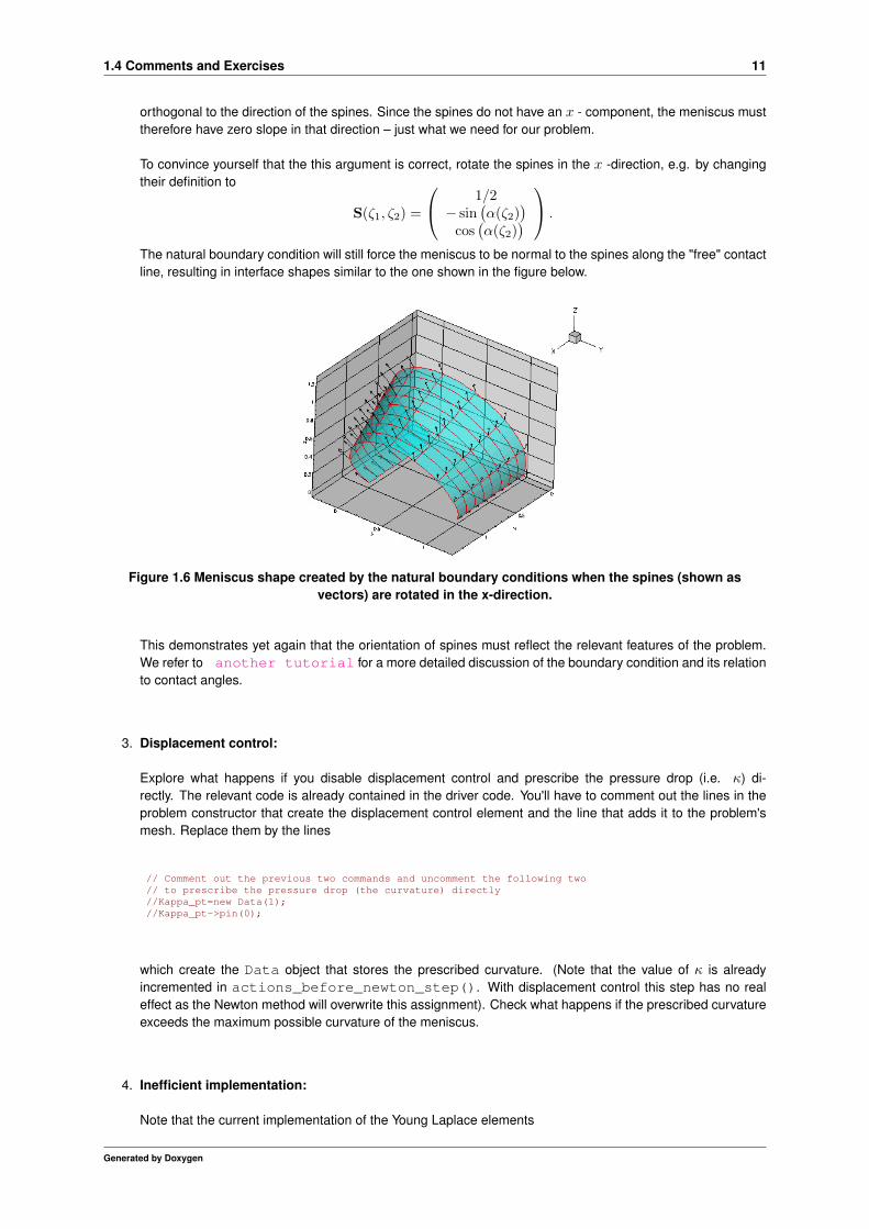
To convince yourself that the this argument is correct, rotate the spines in the x -direction, e.g. by changingtheir definition to

S(ζ1, ζ2) =

1/2− sin

(α(ζ2)

)cos(α(ζ2)

) .

The natural boundary condition will still force the meniscus to be normal to the spines along the "free" contactline, resulting in interface shapes similar to the one shown in the figure below.

Figure 1.6 Meniscus shape created by the natural boundary conditions when the spines (shown asvectors) are rotated in the x-direction.

This demonstrates yet again that the orientation of spines must reflect the relevant features of the problem.We refer to another tutorial for a more detailed discussion of the boundary condition and its relationto contact angles.

3. Displacement control:

Explore what happens if you disable displacement control and prescribe the pressure drop (i.e. κ) di-rectly. The relevant code is already contained in the driver code. You'll have to comment out the lines in theproblem constructor that create the displacement control element and the line that adds it to the problem'smesh. Replace them by the lines

// Comment out the previous two commands and uncomment the following two// to prescribe the pressure drop (the curvature) directly//Kappa_pt=new Data(1);//Kappa_pt->pin(0);

which create the Data object that stores the prescribed curvature. (Note that the value of κ is alreadyincremented in actions_before_newton_step(). With displacement control this step has no realeffect as the Newton method will overwrite this assignment). Check what happens if the prescribed curvatureexceeds the maximum possible curvature of the meniscus.

4. Inefficient implementation:

Note that the current implementation of the Young Laplace elements

Generated by Doxygen

12 Example problem: The Young Laplace equation

is inefficient as the elemental Jacobian matrices are computed by finite-differencing. You are invited toimplement the analytical computation of the Jacobian matrix as an exercise.

5. Other problems:

We provide a number of additional demo driver codes that demonstrate the solution of other, relatedproblems.

• The code

demo_drivers/young_laplace/young_laplace.cc

and its adaptive counterpart

demo_drivers/young_laplace/refineable_young_laplace.cc

demonstrate the solution of three problems: (i) the barrel-shaped meniscus problem already dis-cussed above; (ii) the deformation of a meniscus that is pinned at all four edges of a square tube; and(iii) the solution of a problem with contact-angle boundary conditions. The latter one is discussed in aseparate tutorial.

• The spherical meniscus that emanates from a circular tube, shown in the animation at the beginning ofcurrent document, was computed with:

demo_drivers/young_laplace/spherical_cap_in_cylinder.cc

1.5 Source files for this tutorial

• The source files for this tutorial are located in the directory:

demo_drivers/young_laplace/

• The driver code is:

demo_drivers/young_laplace/barrel.cc

Generated by Doxygen

1.6 PDF file 13

1.6 PDF file

A pdf version of this document is available.

Generated by Doxygen