Examining high level neural representations of cluttered scenes

Computer Science and Artificial Intelligence Laboratory

Technical Report

m a s s a c h u s e t t s i n s t i t u t e o f t e c h n o l o g y, c a m b r i d g e , m a 0 213 9 u s a — w w w. c s a i l . m i t . e d u

MIT-CSAIL-TR-2010-034CBCL-289

July 29, 2010

Examining high level neural representations of cluttered scenes Ethan Meyers, Hamdy Embark, Winrich Freiwald, Thomas Serre, Gabriel Kreiman, and Tomaso Poggio

Examining high level neural representations of cluttered scenes Ethan Meyers1, Hamdy Embark2, Winrich Freiwald2,3, Thomas Serre1,4, Gabriel Kreiman1,5, Tomaso Poggio1

1 Department of Brain and Cognitive Sciences, McGovern Institute, MIT 2 Center for Cognitive Science, Brain Research Institute, University of Bremen 3 Rockefeller University 4 Department of Cognitive & Linguistic Sciences, Brown University 5 Ophthalmology and Program in Neuroscience, Children's Hospital Boston, Harvard Medical School Corresponding author: Ethan Meyers ([email protected]) Abstract Humans and other primates can rapidly categorize objects even when they are embedded in complex visual scenes (Thorpe et al., 1996; Fabre-Thorpe et al., 1998). Studies by Serre et al., 2007 have shown that the ability of humans to detect animals in brief presentations of natural images decreases as the size of the target animal decreases and the amount of clutter increases, and additionally, that a feedforward computational model of the ventral visual system, originally developed to account for physiological properties of neurons, shows a similar pattern of performance. Motivated by these studies, we recorded single and multi unit neural spiking activity from macaque superior temporal sulcus (STS) and anterior inferior temporal cortex (AIT), as a monkey passively viewed images of natural scenes. The stimuli consisted of 600 images of animals in natural scenes, and 600 images of natural scenes without animals in them, captured at four different viewing distances, and were the same images used by Serre et al. to allow for a direct comparison between human psychophysics, computational models, and neural data. To analyze the data, we applied population ‘readout‘ techniques (Hung et al., 2005; Meyers et al., 2008) to decode from the neural activity whether an image contained an animal or not. The decoding results showed a similar pattern of degraded decoding performance with increasing clutter as was seen in the human psychophysics and computational model results. However, overall the decoding accuracies from the neural data lower were than that seen in the computational model, and the latencies of information in IT were long (~125ms) relative to behavioral measures obtained from primates in other studies. Additional tests also showed that the responses of the model units were not capturing several properties of the neural responses, and that detecting animals in cluttered scenes using simple model units based on V1 cells worked almost as well as using more complex model units that were designed to model the responses of IT neurons. While these results suggest AIT might not be the primary brain region involved in this form of rapid categorization, additional studies are needed before drawing strong conclusions.

Introduction Human and other non-human primates are able to rapidly extract information from complex visual scenes. Psychophysics studies have shown that humans can make reliable manual responses indicating whether an animal is present in a visual scene as early as 220ms after stimulus onset (Thorpe et al., 1996; Rousselet et al., 2002; Delorme et al., 2004), and when shown an animal and a non-animal image simultaneously (one in the left and right visual field), humans can reliably initiate saccades to the animal image with latencies as fast as 120ms after stimulus onset (Kirchner and Thorpe, 2006). Additional studies in humans have also shown that this rapid categorization behavior can occur in the absence of attention (Li et al., 2002), that performance is just as accurate when engaging in the task simultaneously in both left and right visual fields (Rousselet et al., 2002), and that categorization accuracy decreases as the amount of clutter in an image increases (and the size of the target decreases) (Serre et al., 2007). Similar studies using macaques have shown similar results although monkeys have even faster reactions times, with manual reaction times as quick as 180-230ms and saccade reaction times as fast as 100ms after stimulus onset (Fabre-Thorpe et al., 1998; Delorme et al., 2000; Macé et al., 2005; Girard et al., 2008). Thus humans and macaques have the ability to rapidly categorize complex and diverse images, potentially in parallel, and seemingly without the need to deploy attention. A few studies have also examined the neural mechanisms that underlie this rapid categorization behavior. Electroencephalography (EEG) studies in humans on animal detection tasks have shown differences in event-related potentials (ERPs) around 150-170ms after stimulus onset between target present and target absent trials (Thorpe et al., 1996; Rousselet et al., 2002; Delorme et al., 2004). Functional magnetic resonance imaging (fMRI) studies in humans have also shown that when subjects need to detect a particular category of object in a scene, patterns of activity BOLD activity in lateral occipital complex (LOC) are similar to the patterns seen when an isolated image of an object from the same category is shown (Peelen et al., 2009). Electrophysiological studies in macaques have also examined the effects that cluttered images have on neural responses and have shown that neurons’ selectivity is not changed when a monkey fixates (and notices) a preferred object in the context of a cluttered scene (Sheinberg and Logothetis, 2001; Rolls et al., 2003). Additionally, studies on the neural basis of categorization have shown a diverse set of areas including the inferior temporal cortex (IT) (Sigala and Logothetis, 2002; Freedman et al., 2003; Kiani et al., 2007; Meyers et al., 2008), the prefrontal cortex (PFC) (Freedman et al., 2000, 2001; Shima et al., 2007), and lateral intraparietal cortex (LIP) (Freedman and Assad, 2006) are involved in different types of categorization behavior. However, these studies have generally used simpler stimuli of isolated objects, and a direct examination of the neural processing that underlies the rapid categorization behavior in complex cluttered images has not been undertaken.

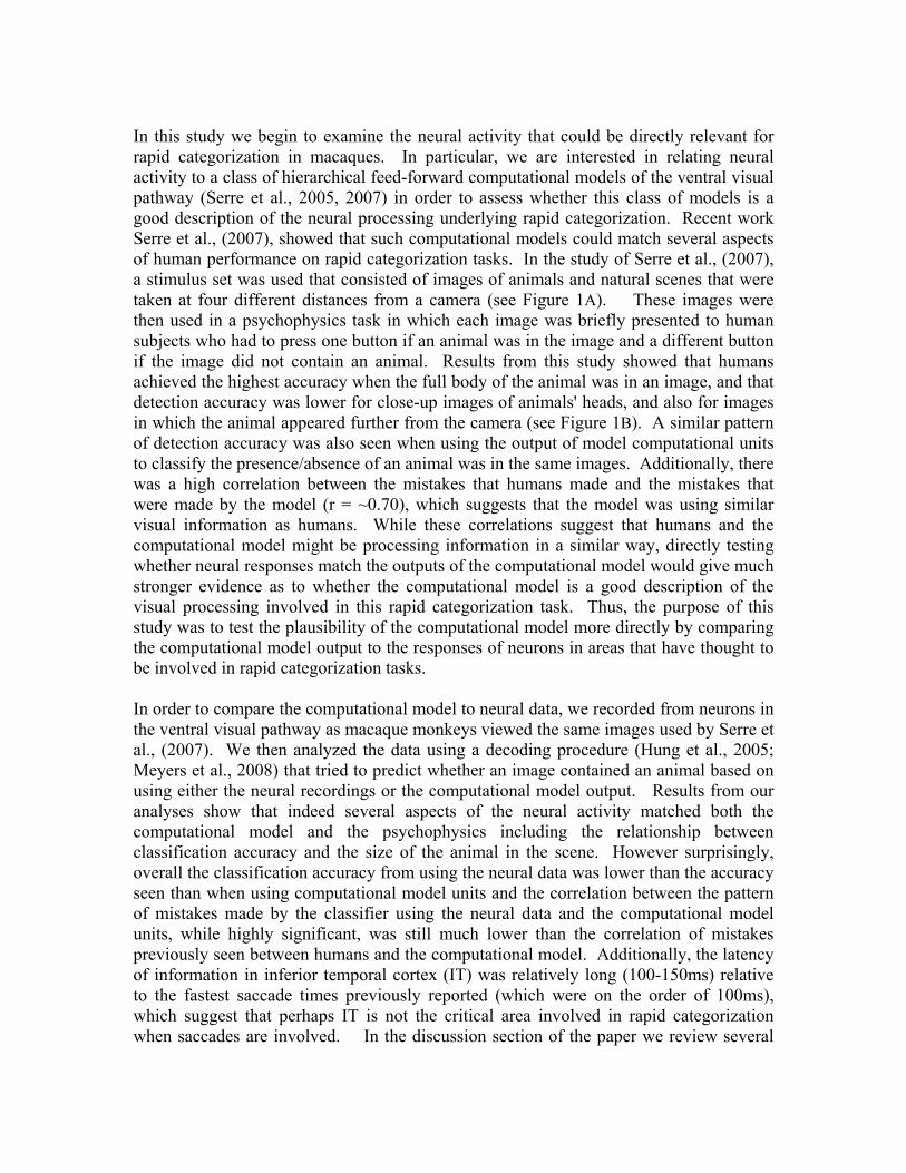
In this study we begin to examine the neural activity that could be directly relevant for rapid categorization in macaques. In particular, we are interested in relating neural activity to a class of hierarchical feed-forward computational models of the ventral visual pathway (Serre et al., 2005, 2007) in order to assess whether this class of models is a good description of the neural processing underlying rapid categorization. Recent work Serre et al., (2007), showed that such computational models could match several aspects of human performance on rapid categorization tasks. In the study of Serre et al., (2007), a stimulus set was used that consisted of images of animals and natural scenes that were taken at four different distances from a camera (see Figure 1A). These images were then used in a psychophysics task in which each image was briefly presented to human subjects who had to press one button if an animal was in the image and a different button if the image did not contain an animal. Results from this study showed that humans achieved the highest accuracy when the full body of the animal was in an image, and that detection accuracy was lower for close-up images of animals' heads, and also for images in which the animal appeared further from the camera (see Figure 1B). A similar pattern of detection accuracy was also seen when using the output of model computational units to classify the presence/absence of an animal was in the same images. Additionally, there was a high correlation between the mistakes that humans made and the mistakes that were made by the model (r = ~0.70), which suggests that the model was using similar visual information as humans. While these correlations suggest that humans and the computational model might be processing information in a similar way, directly testing whether neural responses match the outputs of the computational model would give much stronger evidence as to whether the computational model is a good description of the visual processing involved in this rapid categorization task. Thus, the purpose of this study was to test the plausibility of the computational model more directly by comparing the computational model output to the responses of neurons in areas that have thought to be involved in rapid categorization tasks. In order to compare the computational model to neural data, we recorded from neurons in the ventral visual pathway as macaque monkeys viewed the same images used by Serre et al., (2007). We then analyzed the data using a decoding procedure (Hung et al., 2005; Meyers et al., 2008) that tried to predict whether an image contained an animal based on using either the neural recordings or the computational model output. Results from our analyses show that indeed several aspects of the neural activity matched both the computational model and the psychophysics including the relationship between classification accuracy and the size of the animal in the scene. However surprisingly, overall the classification accuracy from using the neural data was lower than the accuracy seen than when using computational model units and the correlation between the pattern of mistakes made by the classifier using the neural data and the computational model units, while highly significant, was still much lower than the correlation of mistakes previously seen between humans and the computational model. Additionally, the latency of information in inferior temporal cortex (IT) was relatively long (100-150ms) relative to the fastest saccade times previously reported (which were on the order of 100ms), which suggest that perhaps IT is not the critical area involved in rapid categorization when saccades are involved. In the discussion section of the paper we review several

factors could have contributed to these discrepancies in the results between the model and the neural data that could potentially explain our results, however further electrophysiological studies are needed to make more conclusive statements. Methods Subjects and surgery Two male adult rhesus macaque monkeys (referred to as Monkey A and Monkey B) were used in this study. All procedures conformed to local and NIH guidelines, including the NIH Guide for Care and Use of Laboratory Animals as well as regulations for the welfare of experimental animals issued by the German Federal Government. Prior to recording, the monkeys were implanted with ultem headposts (for further details see Wegener et al., 2004) and trained via standard operant conditioning techniques to maintain fixation on a small spot for a juice reward. Recordings and eye-position monitoring Single-unit recording & Eye-position monitoring. We recorded extracellularly with electropolished Tungsten electrodes coated with vinyl lacquer (FHC, Bowdoinham, ME). Extracellular signals were amplified, bandpass filtered (500Hz-2 kHz), fed into a dual-window discriminator (Plexon, Dallas TX) and sorted online. Spike trains were recorded at 1 ms resolution. Quality of unit isolation was monitored by separation of spike waveforms and inter spike interval histograms (ISHs). A total of 116 well isolated single units were recorded from dorsal anterior inferior temporal cortex (AITd) from monkey A, and 256 well isolated single units were recorded from AITd from monkey B. Additionally for monkey A, 444 well isolated units were recorded from dorsal posterior inferior temporal cortex (PITd), and 99 well isolated units were recorded from ventral posterior inferior temporal cortex (PITv). Eye position was monitored with an infrared eye tracking system (ISCAN, Burlington MA) at 60 Hz with an angular resolution of 0.25°, calibrated before and after each recording session by having the monkey fixate dots at the centre and four corners of the monitor. Ophthalmic examination Monkey A's eyes were inspected by one of the experimenters and a trained ophthalmologist with two different ophthalmoscopes. These measurements, performed in the awake and the ketamine anesthetized monkey, revealed myopia on the left (-3 dioptries) and right (-9 dioptries) eyes. In addition signs of astigmatism and possible retinal deficiancies were observed. Stimuli and task

Two sets of stimuli were used in two different experiments. In the ‘animal-scenes’ experiment, the stimuli consisted of 600 images of animals in natural scenes, and 600 images of scenes without animals (see Figure 1A for examples of these stimuli). The animal and scene images were captured at four different distances from a camera, which we will refer to as ‘head’, ‘close-body’, ‘medium-body’ and ‘far-body’ images, which describes how the animals appeared in the different types of images, as determined by a set of human ratings (see Serre et al., 2007 for details). The images used in our experiments are same images as Serre et al., (2007) which allows us to directly compare results from the neural data to previous human psychophysics and computational modeling results. In the second ‘isolated objects’ experiment, the stimuli consisted of 77 images of objects from 8 different categories (food, toys, cars/airplanes, human faces, monkey faces, cats/dogs, boxes, and hands). These stimuli were previously used in a study by Hung et al., (2005), and allowed us to compare our neural data to previous recordings made from anterior IT (see Figure 1C for examples of these stimuli). More details about the stimulus sets can be found in Serre et al., (2007) and in Hung et al., (2005). For both experiments, the stimuli were presented in a rapid sequence, with each stimulus being presented for 100ms, followed by 100ms inter-stimulus-interval in which a gray screen was shown (see Figure 1D). During the presentation of the stimuli, the monkey sat in a dark box with its head rigidly fixed, and was given a juice reward for keeping fixation for 2-5 seconds within a 1.1 degree fixation box (when fixation was not kept, the image sequence during which fixation was not maintained, was repeated). Visual stimuli were presented using custom software (written in Microsoft Visual C/C++), and presented at a 60 Hz monitor refresh rate and 640 x 480 resolution on a 21" CRT monitor. The monitor was positioned 54 cm in front of the monkey's eyes, and the images subtended a 6.4° x 6.4° region of the visual field. For the isolated-objects experiment, all images were presented in random order until 10 presentations of each of the 77 objects had been shown. For the animal-scene experiment, the 1200 images were divided into blocks of 120 images, with each block consisting of 15 animal and 15 scene images from each of the four camera distances. The experiment consisted of running 5 presentations of each image within a block before going on to present the next block. For every experimental session, the blocks were presented in the same order, but the images within each block were fully randomized.

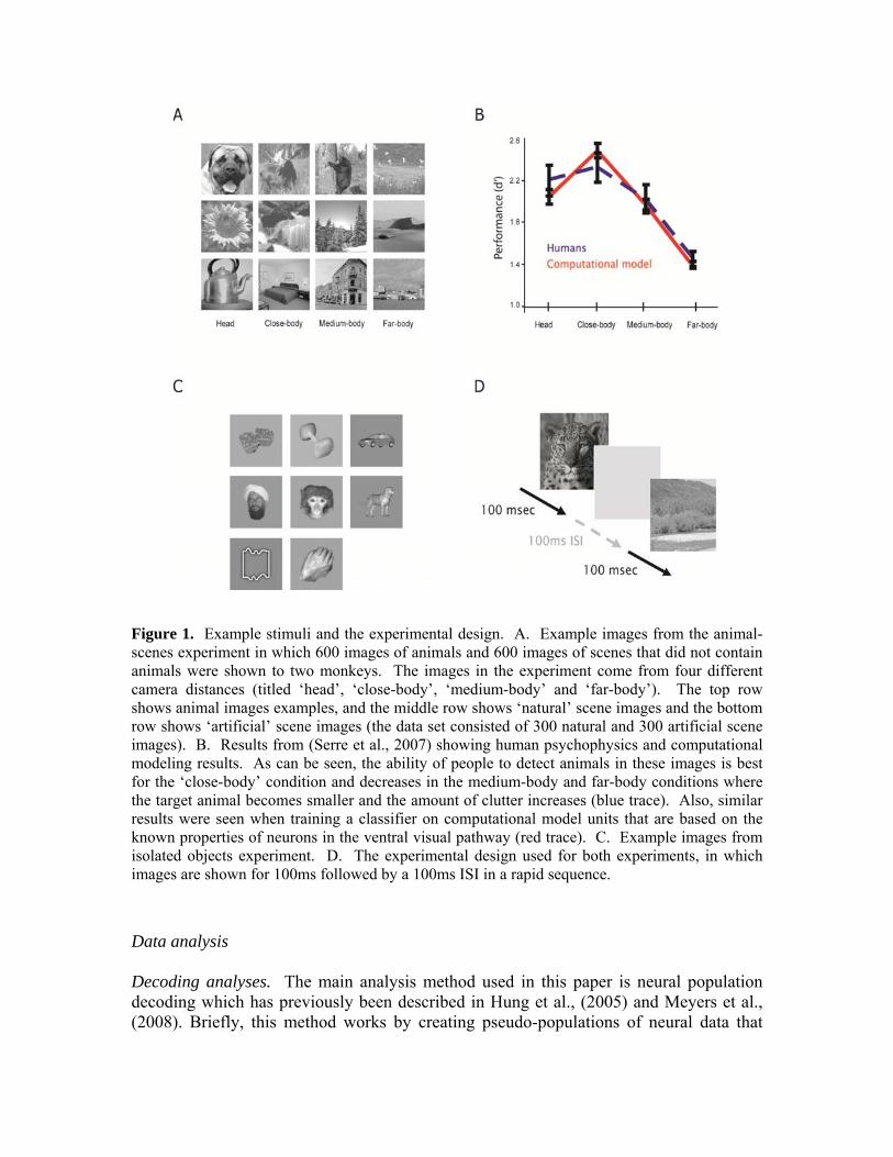
Figure 1. Example stimuli and the experimental design. A. Example images from the animal-scenes experiment in which 600 images of animals and 600 images of scenes that did not contain animals were shown to two monkeys. The images in the experiment come from four different camera distances (titled ‘head’, ‘close-body’, ‘medium-body’ and ‘far-body’). The top row shows animal images examples, and the middle row shows ‘natural’ scene images and the bottom row shows ‘artificial’ scene images (the data set consisted of 300 natural and 300 artificial scene images). B. Results from (Serre et al., 2007) showing human psychophysics and computational modeling results. As can be seen, the ability of people to detect animals in these images is best for the ‘close-body’ condition and decreases in the medium-body and far-body conditions where the target animal becomes smaller and the amount of clutter increases (blue trace). Also, similar results were seen when training a classifier on computational model units that are based on the known properties of neurons in the ventral visual pathway (red trace). C. Example images from isolated objects experiment. D. The experimental design used for both experiments, in which images are shown for 100ms followed by a 100ms ISI in a rapid sequence.

Data analysis Decoding analyses. The main analysis method used in this paper is neural population decoding which has previously been described in Hung et al., (2005) and Meyers et al., (2008). Briefly, this method works by creating pseudo-populations of neural data that

consist of firing rates from a few hundred neurons that were recording independently but are treated as if they had been recorded simultaneously. A pattern classifier is first trained on several examples of these pseudo-population responses for each stimulus type, and then the classifier is used to make predictions about which stimulus type is present in a new set of pseudo-population responses that come from a different set of trials. The classification accuracy is calculated as the percentage of correct predictions made on the test dataset. For decoding which exact image was shown (Supplemental figure 1) the decoding procedure is used in a cross-validation paradigm in which the pseudo-population responses are divided into k sections; k-1 sections of data are used from training the classifier and the last section is used for testing, and the procedure is repeated k times each time using a different section of the data for testing (for supplemental figures 1, there were k=10 splits of the data, with each split consisting of pseudo-population responses from each of the 77 isolated objects). For all analyses, a bootstrap procedure is also applied in which different pseudo-populations are created from the data, and then whole cross-validation procedure is run. In this paper, the bootstrap procedure is run either 50 times for the isolated object analysis, or 250 times for the animal/non-animal analyses, and the final decoding results consist of the average decoding accuracy over all these different bootstrap-like (and cross-validation) runs. The error bars that are plotting are the standard deviation of the classification accuracy statistics calculated over all bootstrap-like runs. Most decoding results in this paper are based on using a maximum correlation coefficient (MCC) classifier (this classifier has also been called a correlation coefficient classifier (Meyers et al., 2008), the maximum correlation classifier (Wilson and McNaughton, 1993) and the dot product algorithm (Rolls et al., 1997) and is described in those papers). We also make use of support vector machines (SVMs), and regularized least squares (RLS) classifiers (Vapnik, 1995; Chang and Lin, 2001; Rifkin and Lippert, 2007). It should be noted that the MCC classifier does not have any ‘free-parameters’ that are not completely fixed by the data, while the SVM and the RLS classifiers have a single free-parameter (called the error penalty parameter and denoted by the letter C)1 that determines the tradeoff between how well the classifier should fit the training data, versus how complex of a function should the classifier use. Larger values of the error penalty parameter C will cause the classifier to use more complex functions that better fit the data, however using a function that is too complex will often hurt the ability to correctly classify new points that are not in the training set (i.e., the classifier will overfit the training data). Conversely, if the value of C is too small, then the classifier will choose a function that is too simple that will not fit the training data very well which will also cause the classifier to generalize poorly to new data. For the RLS classifier, there is an efficient way to find the optimal value of C using only the training data which we always used (for this reason we generally prefer to use an RLS classifier over a SVM; see Rifkin and Lippert, 2007). For other analyses we are interested in comparing our work to previous work that used SVMs, thus we explicitly vary the value of C and see how changes in this parameter affect the cross-validation results (see Figure 6C). It should be

1 It is also common for researchers in machine learning to talk about a ‘regularization constant’ parameter (denoted λ) rather than the error penalty parameter C. The error penalty constant is related to the regularization constant by the formula C = 1/(λ *k), where k is the number of training examples.

noted that in order to make the problem of finding a good value for C computationally tractable when using an SVM, our analyses look at the cross-validation results from changing C rather than optimizing C using only the training data and then applying cross-validation (as is done for the RLS results); thus the classification accuracies from these analyses could be slightly biased upward due to over-fitting. Before the data is passed to the classifier we calculate the mean and standard deviation for each neuron/model-unit using only the training data, and then we z-score normalize the training and test data using these means and standard deviations. The reason for normalizing the data is that the range of firing rates can vary drastically between different neurons, and such normalization helps prevent neurons with high firing rates from dominating the population analysis (although in practice we have found that results are largely unaffected by such normalization). Results from these decoding analyses are reported in two different ways. The first ways is to simply report the ‘classification accuracy’, which is the percentage of the test data points that are correctly classified. The second way we report the results is in terms of the d-prime score. For the animal/no-animal decoding experiment, the d-prime decoding accuracy is calculated as the z-transform of proportion of animal images correctly classified as containing animals minus the z-transform of the proportion of images falsely classified as containing animals. We use this d-prime score in order to be able to easily compared our results to Serre et al., (2007) which also reported their results using this measure. Our main decoding analyses address the question of whether we could use neural data to classify whether an image of a natural scene contains an animal (Figure 2). To do this analysis we use data from 50% of the images for training and data from the remaining 50% of the images for testing, making sure that the data from exactly half the images in both the training and test sets contain animals. Since each unique image was repeated 5 times when shown to the monkey, the data from all five trials for a specific stimulus went into the training set while the test set consisted of a single pseudo-population response from each image - thus the training set consisted of 3000 points and the test set consisted of 600 points2 (using data from only a single trial of each image type for the training set did not change the results, see Supplemental figure 10). Additionally, for each bootstrap-like run, the images in both the training and test sets were divided evenly among the four camera distance image classes (i.e., 25% head, 25% close-body, 25% medium-body and 25% far-body in both the training and test sets), to keep all decoded conditions balanced. When training the classifier, all data from different camera distances was treated the same and a single decision boundary was learned for classifying images that contained animals versus images that did not, exactly replicating the type of analysis done by Serre et al., (2007)). When testing the classifier, the decoding results for the four camera distances are typically reported separately (e.g., Figure 2A, Figure 2B etc.), and for some analyses, the results were further separated into accuracy for the animal images vs. the accuracy for

2 In retrospect it might have been better to use all 5 repetitions of the test points as well, which could have possibly led to slightly smoother results and smaller errorbars, although the results overall would be very similar.

the scene images (e.g., Figure 3). For all analysis, the decoding procedure was repeated 250 times using different images of animals/scenes in the training and test set each time. In order to calculate the latency of information in AITd, we used a permutation test to assess when the decoding accuracies exceeded a level that would be expected by chance (Golland and Fischl, 2003). For each 25ms time bin that was used in Figure 2C, we randomly shuffled the image labels, and applied the full cross-validation decoding procedure using 50 bootstrap-like iterations3. This whole procedure was repeated 250 times to give a null distribution which indicates the range of expected decoding values obtained if there was no real relationship between the images shown and the data collected. P-values were calculated as the proportion of samples in the null distribution that were greater than or equal to the decoding accuracy from the real data-label pairing. The latency of information was then assigned to the first 25ms bin in which the p-values were below p = 0.05 level. Comparison to computational model units and human psychophysics results. In some of the analyses we compare results from decoding neural activity to the results obtained from decoding the outputs of computational model units of Serre et al., (2007) that were run on the same animal/scene images. Briefly, the model of Serre et al., (2007) consists of a sequence of processing stages that alternate between template matching operations (which give rise to S units) and maximum operations (which give rise to C units), and works as follows: On the first level (the S1 level) images are convolved with a set of Gabor filters at four different orientations and 16 different spatial scales at locations distributed evenly across the image to create a larger vector of responses (these responses are analogous to the output of V1 simple cells). Next, for each S1 orientation, the maximum S1 response value within a small spatial neighborhood and over adjacent scales is taken to create a C1 vector of responses (these responses are analogous to the output of V1 complex cells). On the next level (the S2 level), for each local neighborhood, C1 unit response are compared to a number of ‘templates’ vectors (these template vectors were previously extracted from running the C1 model on a random subset of natural images that were not used in these experiments); the S2 response vector then consists of the correlation between each template vector and each C1 neighborhood response. For each template vector, the maximum value of S2 unit within a larger neighborhood is then taken to create the C2 responses (these C2 responses have been previously compared to the responses of V4 units by (Cadieu et al., 2007). Likewise S3 responses are created by comparing C2 responses to another set of templates, and C3 responses are created by pooling over even larger neighborhoods of S3 units. For more details on the model see Serre et al., (2007). Analysis of the outputs of the computational model units was done by applying the exact same decoding procedure that was used to decode the neural data except the neural responses were replaced by the responses of computational units. Unless otherwise specified in the text, the exact same

3 Ideally we would have run 250 bootstrap trials for each sample in the null-distribution to match the 250 bootstrap runs used to create the real decoding results, however this was computationally too expensive. Using only 50 bootstraps for each null sample will make each sample point in the null distribution slightly more variable, which will lead to a slightly larger standard deviation in the null distribution and consequently to more conservative p-values (i.e., more likely to make type II errors than type I error).

number of computational model units and of neural responses were always compared in order to make the comparison of results are closely matched as possible. Human psychophysics experiments were also previously run (Serre et al., 2007) using the same images that were used in the electrophysiological experiments reported in this paper. In those experiments, images were flashed for 20ms on a screen followed by a 30ms black screen inter-stimulus interval which was then followed by an 80ms mask, and humans needed to report whether an animal was present in the images. For several analyses in the paper, we compare the accuracy that humans could detect animals in specific images to the accuracy that a classifier achieved in detecting an animal in a specific image based on either neural data or data from computational model units. Comparing the computational model units to the neural data was done in several ways. The simplest way to do this comparison was to plot the classification accuracies from the computational model units next to the classification accuracies from the neural data (Figure 2 and Figure 3). In order to do more detailed comparisons, two other methods were used. In the first method, we compared neural population activity to populations of computational model units by examining which images were consistently classified as animals (regardless of whether the classification was correct) using either neural data or computation model data as input to the classifier. To do this analysis we ran the decoding procedure 250 times, and calculated how often each of the 1200 images was classified as an animal. This yielded a 1200 dimensional ‘animal-prediction’ vector for both the neural and computational model data. We then correlated the animal-prediction vector derived from the neural data to the animal-prediction vector derived from computational model unit predictions to get an estimate of whether the neural data and the model units were making the same pattern of predictions (this again is similar to an analysis done by Serre et al., (2007) in order to compare human psychophysics performance on an animal detection task to the performance of computational model units). Additionally, we calculated the correlation between the animal-prediction vectors from each monkey, to get a baseline to compare the computational model animal predictions to. We also compare animal-prediction results from Serre et al., (2007) based on mistakes humans made on an animal detection psychophysics task and based on a ‘full’ computational model consisting of 6000 model units that was used in that work. Results are reported using both Pearson’s correlation coefficient and Spearman’s correlation coefficient. In order to assess whether any of the correlations between these animal-prediction vectors could have occurred by chance, we conducted a permutation test. This test was done by randomly permuting the values each 1200 element animal-prediction vector and then calculating the correlation values in these permuted vectors. The permutation procedure was repeated 1000 times to create null-distributions for each correlation pair, and the p-value was assessed as the proportion of values in the null distribution that were greater than the correlation values from the real unperturbed animal-prediction vectors. For all comparisons made in Table 1, all the real correlation values were greater than any value in the null distribution, indicating that each correlation was beyond what would be expected by chance. Approximate 95 percent confidence intervals were also calculated

for the Pearson and Spearman correlation values on this null distribution by taking the 25th lowest and 976th highest values for all pairs of conditions that were correlated, and then choosing the pair that had the minimum value for the lower bound and the pair that had the maximum value as upper bound yielding a conservative estimate for the 95% confidence interval for all pairs (in practice the 95% confidence interval was in fact quite similar between all pairs). We also compared the computational model units decoding results to the decoding results obtained from other simpler visual features. These features were: S1 model units (which are just Gabor filters created at four different orientations and 16 different scales), randomly chosen pixels, and the mean values of pixels in small image patches. To create the S1 units, we used the parameters previously described by (Serre et al., 2007), and then selected randomly 1600 units for each of the four orientations of Gabor filters, yielding a pool of 6400 features for each image (the same filters were chosen for all the images, thus making the decoding possible). To create the pixel representation, 1600 randomly selected pixels were chosen from each image (again, the position of each randomly selected pixel was the same in all of the images). To create the mean patch representation, we used a similar process that was used to create the S1 units, except that we convolved the image with averaging filters at 16 different patch sizes rather than Gabor functions, and there was only a total of 1600 features used, since mean filters are not oriented. When decoding whether an image contained an animal in it using these features, we applied the same decoding procedure that was used for model units and neural data; namely, on each bootstrap-like iteration, we randomly selected 100 features from the larger pool, and then repeated this bootstrap-like procedure 250 times using a different selection of 100 random features each time. Results Decoding whether an animal is in a natural scene image To try to gain a better understanding of the brain regions and neural processing that underlies rapid object recognition, we used a population decoding approach to assess if we can predict whether an animal was present in a complex natural scene image that was shown to a monkey based on neural data recorded from the ventral visual stream. If it is possible to decode whether an animal is in a complex natural scene image from neural data from AIT recorded <100ms after stimulus onset, then this suggests that AIT could potentially be an important brain region in rapid categorization behavior. Alternatively, if it is not possible to decode whether an animal is in a natural scene image within a behaviorally relevant time period, this gives some support to the theory that other brain regions might be the critical areas involved in rapid categorization (Kirchner and Thorpe, 2006; Girard et al., 2008). In order to do an animal/non-animal decoding analysis, we trained a classifier using data that was collected from half of the animal and scene images, and we tested the classifier using data that was recorded when the other half the images had been shown (i.e., the

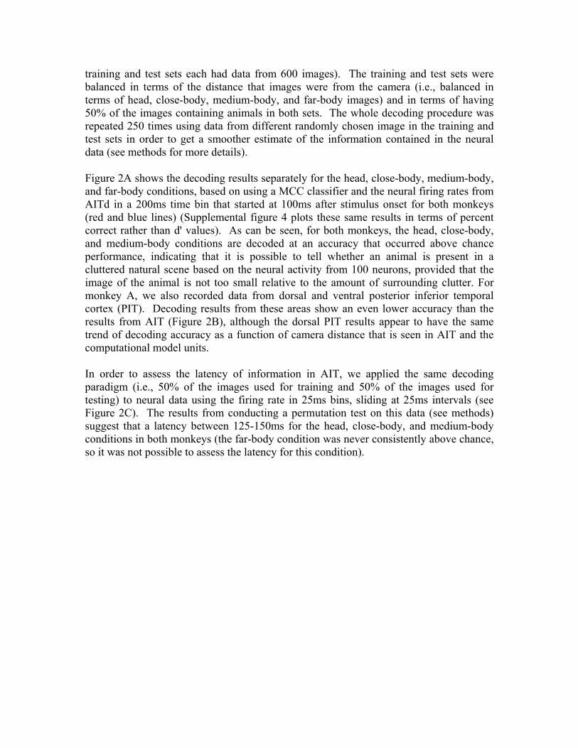
training and test sets each had data from 600 images). The training and test sets were balanced in terms of the distance that images were from the camera (i.e., balanced in terms of head, close-body, medium-body, and far-body images) and in terms of having 50% of the images containing animals in both sets. The whole decoding procedure was repeated 250 times using data from different randomly chosen image in the training and test sets in order to get a smoother estimate of the information contained in the neural data (see methods for more details). Figure 2A shows the decoding results separately for the head, close-body, medium-body, and far-body conditions, based on using a MCC classifier and the neural firing rates from AITd in a 200ms time bin that started at 100ms after stimulus onset for both monkeys (red and blue lines) (Supplemental figure 4 plots these same results in terms of percent correct rather than d' values). As can be seen, for both monkeys, the head, close-body, and medium-body conditions are decoded at an accuracy that occurred above chance performance, indicating that it is possible to tell whether an animal is present in a cluttered natural scene based on the neural activity from 100 neurons, provided that the image of the animal is not too small relative to the amount of surrounding clutter. For monkey A, we also recorded data from dorsal and ventral posterior inferior temporal cortex (PIT). Decoding results from these areas show an even lower accuracy than the results from AIT (Figure 2B), although the dorsal PIT results appear to have the same trend of decoding accuracy as a function of camera distance that is seen in AIT and the computational model units. In order to assess the latency of information in AIT, we applied the same decoding paradigm (i.e., 50% of the images used for training and 50% of the images used for testing) to neural data using the firing rate in 25ms bins, sliding at 25ms intervals (see Figure 2C). The results from conducting a permutation test on this data (see methods) suggest that a latency between 125-150ms for the head, close-body, and medium-body conditions in both monkeys (the far-body condition was never consistently above chance, so it was not possible to assess the latency for this condition).

Figure 2. Results from decoding whether an animal is in a natural scene image using data. A. A comparison of decoding results using neural data from AITd from the two monkeys (red and blue traces), to results obtained from two different types of computational model units (cyan and green traces). As can be seen, decoding results based on the neural data and the computational model units show the same general trend as a function of camera distance. However, overall the decoding accuracies from the computational model units are better than the results from the neural data. B. A comparison of results from three different brain regions from monkey A. The results again show similar trends as a function of camera distance, but the AITd results are better than the more posterior regions. C. Decoding accuracies from both monkeys as a function of time. The colored lines below the plot show time when the results were significantly above chance (p < 0.05 light trances, p < 0.01 dark traces, permutation test). For both monkeys, for the head, close-body and medium-body distance, a significant amount of information was in AITd starting 125-150ms after stimulus onset.

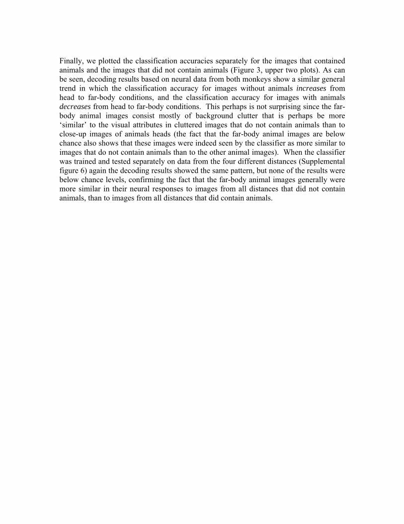
Finally, we plotted the classification accuracies separately for the images that contained animals and the images that did not contain animals (Figure 3, upper two plots). As can be seen, decoding results based on neural data from both monkeys show a similar general trend in which the classification accuracy for images without animals increases from head to far-body conditions, and the classification accuracy for images with animals decreases from head to far-body conditions. This perhaps is not surprising since the far-body animal images consist mostly of background clutter that is perhaps be more ‘similar’ to the visual attributes in cluttered images that do not contain animals than to close-up images of animals heads (the fact that the far-body animal images are below chance also shows that these images were indeed seen by the classifier as more similar to images that do not contain animals than to the other animal images). When the classifier was trained and tested separately on data from the four different distances (Supplemental figure 6) again the decoding results showed the same pattern, but none of the results were below chance levels, confirming the fact that the far-body animal images generally were more similar in their neural responses to images from all distances that did not contain animals, than to images from all distances that did contain animals.

Figure 3. Decoding accuracies using neural and model unit data plotted separately for the animal images (solid lines) and non-animal images (dashed-lines). As can be seen, the results for the neural data from both monkeys (upper two plots) and for the C3 and C2b computational model units (lower two plots) show similar trends with an increase in decoding accuracy for the non-animal images at further camera distances, and a decrease in decoding accuracy for animal images at further camera distances. This pattern of results is due to the fact that the when the animal is far from the camera the background clutter dominates the image causing the computational and neural representations to be more similar to images that do not contain animals.

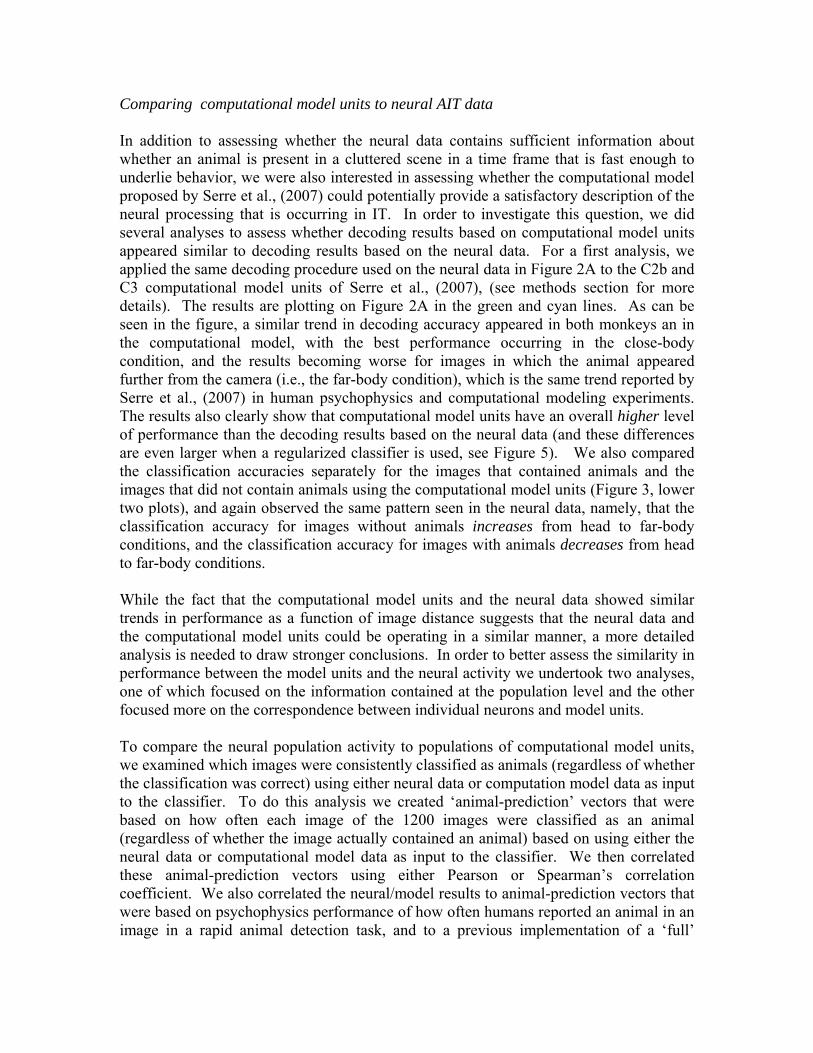
Comparing computational model units to neural AIT data In addition to assessing whether the neural data contains sufficient information about whether an animal is present in a cluttered scene in a time frame that is fast enough to underlie behavior, we were also interested in assessing whether the computational model proposed by Serre et al., (2007) could potentially provide a satisfactory description of the neural processing that is occurring in IT. In order to investigate this question, we did several analyses to assess whether decoding results based on computational model units appeared similar to decoding results based on the neural data. For a first analysis, we applied the same decoding procedure used on the neural data in Figure 2A to the C2b and C3 computational model units of Serre et al., (2007), (see methods section for more details). The results are plotting on Figure 2A in the green and cyan lines. As can be seen in the figure, a similar trend in decoding accuracy appeared in both monkeys an in the computational model, with the best performance occurring in the close-body condition, and the results becoming worse for images in which the animal appeared further from the camera (i.e., the far-body condition), which is the same trend reported by Serre et al., (2007) in human psychophysics and computational modeling experiments. The results also clearly show that computational model units have an overall higher level of performance than the decoding results based on the neural data (and these differences are even larger when a regularized classifier is used, see Figure 5). We also compared the classification accuracies separately for the images that contained animals and the images that did not contain animals using the computational model units (Figure 3, lower two plots), and again observed the same pattern seen in the neural data, namely, that the classification accuracy for images without animals increases from head to far-body conditions, and the classification accuracy for images with animals decreases from head to far-body conditions. While the fact that the computational model units and the neural data showed similar trends in performance as a function of image distance suggests that the neural data and the computational model units could be operating in a similar manner, a more detailed analysis is needed to draw stronger conclusions. In order to better assess the similarity in performance between the model units and the neural activity we undertook two analyses, one of which focused on the information contained at the population level and the other focused more on the correspondence between individual neurons and model units. To compare the neural population activity to populations of computational model units, we examined which images were consistently classified as animals (regardless of whether the classification was correct) using either neural data or computation model data as input to the classifier. To do this analysis we created ‘animal-prediction’ vectors that were based on how often each image of the 1200 images were classified as an animal (regardless of whether the image actually contained an animal) based on using either the neural data or computational model data as input to the classifier. We then correlated these animal-prediction vectors using either Pearson or Spearman’s correlation coefficient. We also correlated the neural/model results to animal-prediction vectors that were based on psychophysics performance of how often humans reported an animal in an image in a rapid animal detection task, and to a previous implementation of a ‘full’

computational model results that was used by Serre et al., (2007) which were obtained by applying an SVM to 1500 units from C1, C2, C2b and C3 levels of the model (for a total of 6000 units). Table 1 shows the results from this analysis using Pearson’s correlation coefficient (upper triangular part of the matrix) or Spearman’s correlation coefficient (lower triangular part of the matrix) (correlations with additional features are shown in supplemental table 4). Based on a permutation test (see methods section), an approximate 95% confidence interval on the Pearson's (Spearman's) correlation from the null distribution is [-0.062 0.062] ([-0.061 0.061]) for all conditions, indicating that all the correlation between animal-predictions for all conditions are well above what would be expected by chance4. Thus the decoding results based on neural data, the computational model and the results of human psychophysics detections are all making similar patterns of mistakes on many images. However, the correlation level between the model units and the neural data is lower than the correlation level between the neural data from the two monkeys5, which suggests that there is additional structure in the neural data that the computation model units are not capturing. Additionally, the correlation between the results obtained from the full computational model of Serre et al., (2007) and the results from using a subset of 100 model units from the higher levels of the computational model (C2b and C3) only have an agreement at a correlation level between .45 and .61. In the section below titled ‘A closer examination of the computational model results’ we examine reasons for this seemingly low correlation.

4 To put the values in Table 1 in perspective, we also calculated two measures of reliability of the neural data by comparing half the data from one monkey to the other half of the data from the same monkey. The first measure of within monkey reliability examined reliability across trials. To do this analysis we randomly divided the neural data from the 5 repeated trials of each stimulus into disjoint two sets, with each set having data from 2 of the trials for each stimulus. We then applied the full decoding procedure to each set of two trials separately, and correlated the animal prediction vectors from the first set with the animal prediction vectors obtained from the second set. Finally this procedure was repeated 50 times. The average Pearson's (Spearman's) correlation value for Monkey A from this procedure was .71 (.70) and the average Pearson's (Spearman's) correlation values from Monkey B were .65 (.62). The second measure of within monkey reliability examined the reliability across neurons. For this analysis we randomly divided the neurons from one monkey into two disjoint sets of 50 neurons each, and then applied the full decoding procedure two each set separately and then correlated the animal prediction vectors. This procedure was also repeated 50 times. The average Pearson (Spearman) correlation value for this procedure for Monkey A was .66 (.62) and for Monkey B was .36 (.35). Thus relative to the comparisons between monkeys and between monkey and computational units, the within monkey reliability was typically high. 5 A 95% confidence interval on the Pearson's correlation between the two monkeys is [.38 .47], while the 95% confidence intervals between Monkey A and the C2b and C3 units are [.21 .31] and [.15 .26] respectively, and the 95% confidence intervals between Monkey B and the C2b and C3 units are [.29 .39] and [.21 .32] respectively. Thus, the confidence intervals on the Pearson's correlation coefficient between the two monkeys only overlaps with the confidence interval between Monkey B and the C2b, which suggests that the agreement between Monkey A and the computational model units, and the agreement between Monkey B and the C3 units, are not as high as the agreement between Monkey A and Monkey B.

Monkey A Monkey B C2b C3 Human Serre full model

Monkey A 0.43 0.26 0.21 0.38 0.36 Monkey B 0.45 0.34 0.27 0.50 0.44 C2b 0.28 0.36 0.91 0.50 0.56 C3 0.21 0.29 0.93 0.40 0.45 Human 0.37 0.48 0.50 0.42 0.72 Serre full model 0.36 0.44 0.61 0.50 0.71

Table 1. Correlation coefficient values between how often each of the 1200 images were predicted as containing an animal based on using human psychophysics results, classification accuracies from neural or computational model units. Upper triangular results are based on Pearson’s correlation coefficient and lower triangular results are based on Spearman’s correlation coefficient. While all the correlation values are larger than would be predicted by chance, higher correlation levels occur between the two monkeys than between the monkeys and computational model units, indicating that the computational model units are not capturing all the possible variance found in the neural data.

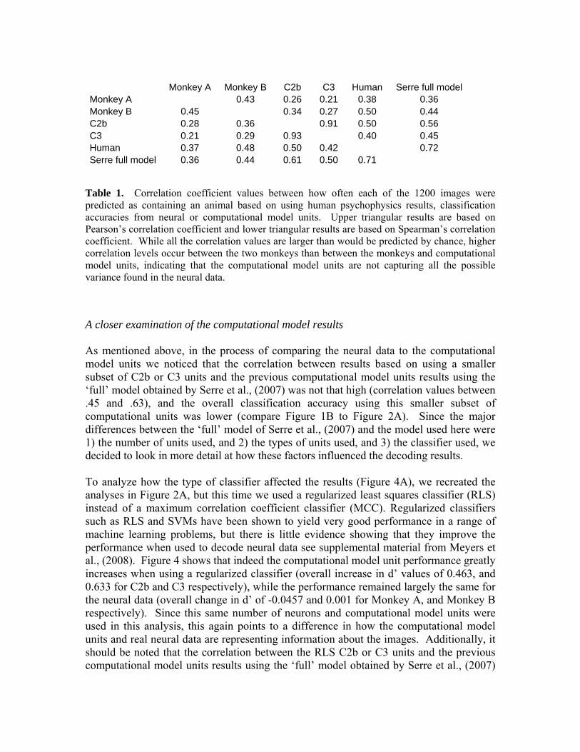
A closer examination of the computational model results As mentioned above, in the process of comparing the neural data to the computational model units we noticed that the correlation between results based on using a smaller subset of C2b or C3 units and the previous computational model units results using the ‘full’ model obtained by Serre et al., (2007) was not that high (correlation values between .45 and .63), and the overall classification accuracy using this smaller subset of computational units was lower (compare Figure 1B to Figure 2A). Since the major differences between the ‘full’ model of Serre et al., (2007) and the model used here were 1) the number of units used, and 2) the types of units used, and 3) the classifier used, we decided to look in more detail at how these factors influenced the decoding results. To analyze how the type of classifier affected the results (Figure 4A), we recreated the analyses in Figure 2A, but this time we used a regularized least squares classifier (RLS) instead of a maximum correlation coefficient classifier (MCC). Regularized classifiers such as RLS and SVMs have been shown to yield very good performance in a range of machine learning problems, but there is little evidence showing that they improve the performance when used to decode neural data see supplemental material from Meyers et al., (2008). Figure 4 shows that indeed the computational model unit performance greatly increases when using a regularized classifier (overall increase in d’ values of 0.463, and 0.633 for C2b and C3 respectively), while the performance remained largely the same for the neural data (overall change in d’ of -0.0457 and 0.001 for Monkey A, and Monkey B respectively). Since this same number of neurons and computational model units were used in this analysis, this again points to a difference in how the computational model units and real neural data are representing information about the images. Additionally, it should be noted that the correlation between the RLS C2b or C3 units and the previous computational model units results using the ‘full’ model obtained by Serre et al., (2007)

was in the range of ~.75 to .78 (see table 2) indicating the type of classifier was a significant factor influencing the difference between our current results and the previous results of Serre et al., (2007). Finally, it should be pointed out that when using an RLS classifier, the Spearman’s correlation between Monkey B and the computational model units is actually higher than the correlation between Monkey A and Monkey B, indicating that model units are capturing as much of the variation in the neural data of Monkey B as should be expected. However the results based on Pearson’s correlation and the correlation between the model units and Monkey B, are still lower than the correlation between the two monkeys indicating that the model units are still not explaining all potential neural variation.

Figure 4. Decoding accuracies for whether an animal is in a cluttered scene image using a regularized least squares (RLS) classifier. A: Results plotted in the same format as Figure 2A, except that a RLS classifier is used instead of an MCC classifier. B: The change in d’ classification accuracy when using a RLS classifier compared to when using an MCC classifier (values calculated by subtracting the MCC decoding accuracies in Figure 2A from the RLS classification accuracies shown in Figure 4A). As can be seen, using a regularized classifier greatly improves the classification performance of the computational model units, while leaving the neural decoding results largely unchanged.

Monkey A Monkey B Model C2b Model C3 Human Serre full model

Monkey A 0.49 0.36 0.36 0.41 0.39Monkey B 0.47 0.44 0.45 0.51 0.44C2b 0.37 0.46 0.95 0.66 0.77C3 0.36 0.47 0.93 0.66 0.75Human 0.39 0.49 0.66 0.65 0.72Serre full model 0.38 0.45 0.77 0.76 0.71

Table 2. Correlation coefficient values between how often each of the 1200 images were predicted as containing animals based on using human psychophysics results, classification accuracies from neural or computational model units when an RLS classifier was used. Upper triangular results are based on Pearson’s correlation coefficient and lower triangular results are based on Spearman’s correlation coefficient. For Pearson’s correlation, the agreement between the two monkeys is still higher than the agreement between the model units and data from either monkey. However, when Spearman’s correlation is used, the neural decoding results from monkey B seem to be better explained by the computational model units than by matching the results to the other monkey (as can be seen by comparing the value in column 1 row 2, with the values in column 2).

To analyze how the number and type of computational model units affected the decoding accuracy, we trained a MCC and a RLS classifier on C1, C2, C2b, C3, and a random combination of all unit types, using either 100 or 1500 units. The results are shown in Figure 5. As can be seen again, results from the RLS classifier are significantly higher than the results from the MCC classifier. There is also an increase in decoding accuracy with more units when an RLS classifier is used, but this increase is somewhat small. More surprisingly, there does not appear to be a clear advantage to using the more sophisticated C2b and C3 features that are supposed to model the responses of IT neurons, compared to the results based on using simple C1 features which are modeled after V1 complex cells (the one exception seems to be for the ‘head’ condition when an MCC classifier is used, for which the C2b and the mix of all unit types tend to perform better than the C1, C2 and C3 units). The fact that C1 units work almost as well as using a combination of all unit types differs from the findings of Serre et al., (2007) which showed that Model C1 units have a lower level of performance than the full Model (see Serre et al., (2007), supplemental table 2). Two differences exist between the methods used here and those used by Serre et al., (2007). First, we used an RLS classifier here, while Serre et al., (2007) used an SVM. Second, Serre et al., (2007) used 1500 Model C1 units and 6000 units of all types in their ‘full’ model, while we used 1500 Model C1 units, and 1500 randomly chosen units of all types in our comparison. Thus either the classifier type of the number of model units used in the ‘full’ model should account for the difference in our findings. Below we explore these two possibilities.

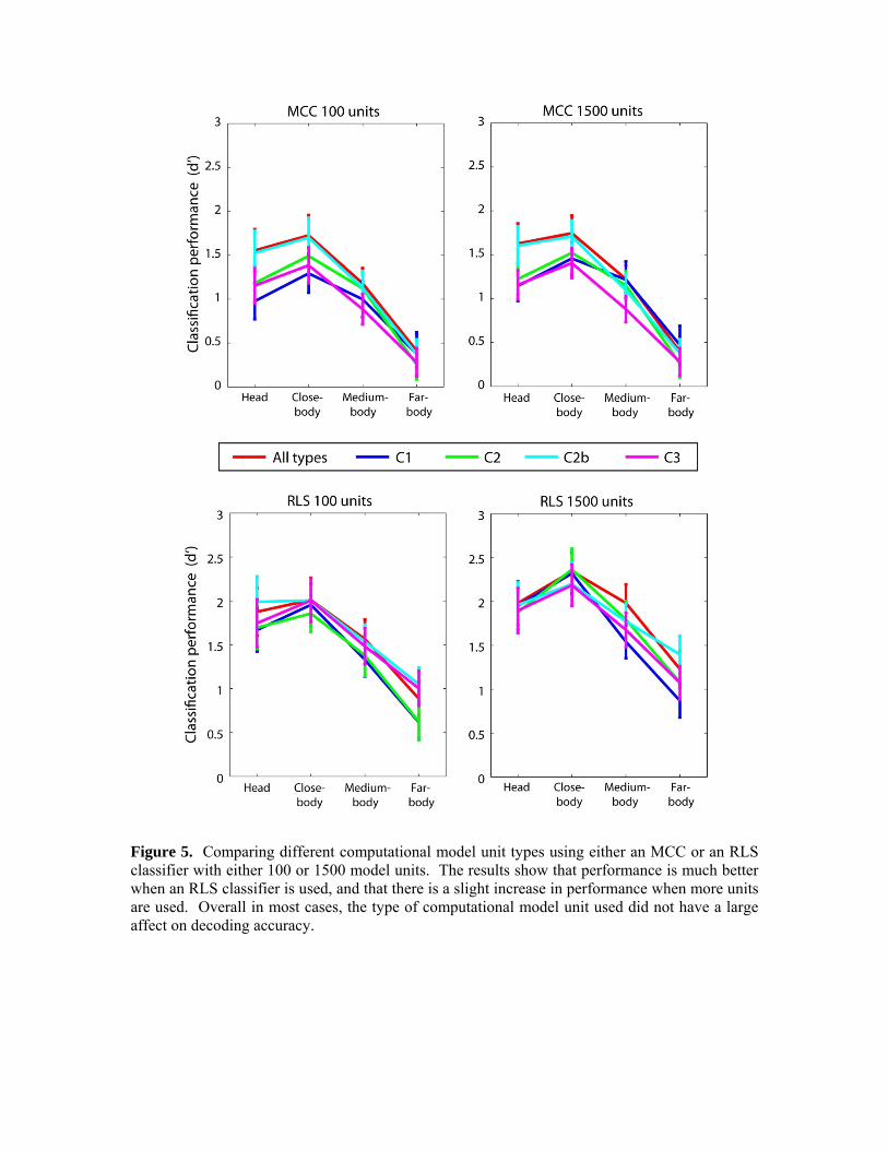
Figure 5. Comparing different computational model unit types using either an MCC or an RLS classifier with either 100 or 1500 model units. The results show that performance is much better when an RLS classifier is used, and that there is a slight increase in performance when more units are used. Overall in most cases, the type of computational model unit used did not have a large affect on decoding accuracy.

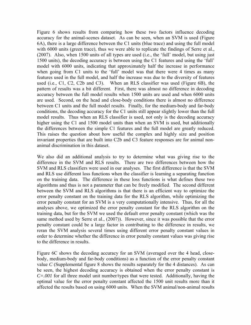
Figure 6 shows results from comparing how these two factors influence decoding accuracy for the animal-scenes dataset. As can be seen, when an SVM is used (Figure 6A), there is a large difference between the C1 units (blue trace) and using the full model with 6000 units (green trace), thus we were able to replicate the findings of Serre et al., (2007). Also, when 1500 units of all types are used (i.e., the ‘full’ model, but using just 1500 units), the decoding accuracy is between using the C1 features and using the ‘full’ model with 6000 units, indicating that approximately half the increase in performance when going from C1 units to the ‘full’ model was that there were 4 times as many features used in the full model, and half the increase was due to the diversity of features used (i.e., C1, C2, C2b and C3). When an RLS classifier was used (Figure 6B), the pattern of results was a bit different. First, there was almost no difference in decoding accuracy between the full model results when 1500 units are used and when 6000 units are used. Second, on the head and close-body conditions there is almost no difference between C1 units and the full model results. Finally, for the medium-body and far-body conditions, the decoding accuracy for the C1 units still appear slightly lower than the full model results. Thus when an RLS classifier is used, not only is the decoding accuracy higher using the C1 and 1500 model units than when an SVM is used, but additionally the differences between the simple C1 features and the full model are greatly reduced. This raises the question about how useful the complex and highly size and position invariant properties that are built into C2b and C3 feature responses are for animal non-animal discrimination in this dataset. We also did an additional analysis to try to determine what was giving rise to the difference in the SVM and RLS results. There are two differences between how the SVM and RLS classifiers were used in our analyses. The first difference is that the SVM and RLS use different loss functions when the classifier is learning a separating function on the training data. The difference in these loss functions is what defines these two algorithms and thus is not a parameter that can be freely modified. The second different between the SVM and RLS algorithms is that there is an efficient way to optimize the error penalty constant on the training data for the RLS algorithm, while optimizing the error penalty constant for an SVM is a very computationally intensive. Thus, for all the analyses above, we optimized the error penalty constant for the RLS algorithm on the training data, but for the SVM we used the default error penalty constant (which was the same method used by Serre et al., (2007)). However, since it was possible that the error penalty constant could be a large factor in contributing to the difference in results, we reran the SVM analysis several times using different error penalty constant values in order to determine whether the difference in error penalty constant values was giving rise to the difference in results. Figure 6C shows the decoding accuracy for an SVM (averaged over the 4 head, close-body, medium-body and far-body conditions) as a function of the error penalty constant value C (Supplemental figure 8 shows the results separately for the 4 distances). As can be seen, the highest decoding accuracy is obtained when the error penalty constant is C=.001 for all three model unit number/types that were tested. Additionally, having the optimal value for the error penalty constant affected the 1500 unit results more than it affected the results based on using 6000 units. When the SVM animal/non-animal results

were recalculated using this optimal value of C=.001 (Figure 6D), the SVM results were a much closer match to the RLS results, indicating that the difference in error penalty constant values was a large factor contributing to the difference in the SVM and RLS results. More importantly, with this optimized error penalty constant value, the head and close-body conditions were no longer higher using all model unit types compared to when only using C1 features. These results indicate that for the animal-scene dataset used in this study that: 1) the model unit results (unlike the results based on neural data) are very sensitive to the exact classifier parameters used, and 2) while using a combination of more complex visual features in the higher model units as well as lower level units does lead to an improvement in discriminating between animals and natural scenes this improvement is smaller than is suggested by Serre et al. (2007) (and seems nonexistent for close-body conditions).

Figure 6. Comparison of using many model unit types, to using only C1 units, for an SVM classifier and a RLS classifier. A: results based on using an SVM (with the default error penalty constant value C =1), yields better performance when the full model using 6000 unit are used compared to using just 1500 C1 features, thus replicating the findings of Serre et al., (2007). When 1500 units of all types are used with a SVM, the results are between the C1 results and the 6000 model unit results of all types, indicating that part of the reason why the ‘full’ model of Serre et al., (2007) outperformed the C1 units was due to the fact that Serre’s full model used four times as many units. B: For the RLS classifier, there is not much difference between using 1500 model units of all types and 6000 model units of all types. Additionally, the C1 units seem to only perform worse on the medium-body and far-body conditions. C: SVM animal/non-animal classification results (averaged over all 4 image distances), as a function of the error penalty parameter C (for all the RLS results, the optimal value of C was always determined using the training data). As can be seen the optimal value of C is .001, which yields higher performance than using the libSVM default value of C = 1. D: SVM animal/non-animal decoding results using an error penalty parameter of C = .001 (that we determined to be optimal in Figure 6C). With this error penalty parameter, the SVM results look much more similar to the RLS results shown in Figure 7B.

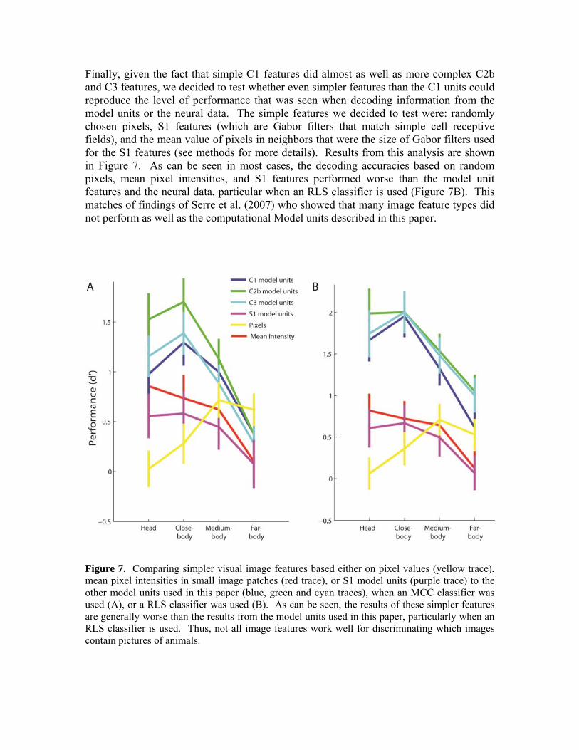
Finally, given the fact that simple C1 features did almost as well as more complex C2b and C3 features, we decided to test whether even simpler features than the C1 units could reproduce the level of performance that was seen when decoding information from the model units or the neural data. The simple features we decided to test were: randomly chosen pixels, S1 features (which are Gabor filters that match simple cell receptive fields), and the mean value of pixels in neighbors that were the size of Gabor filters used for the S1 features (see methods for more details). Results from this analysis are shown in Figure 7. As can be seen in most cases, the decoding accuracies based on random pixels, mean pixel intensities, and S1 features performed worse than the model unit features and the neural data, particular when an RLS classifier is used (Figure 7B). This matches of findings of Serre et al. (2007) who showed that many image feature types did not perform as well as the computational Model units described in this paper.

Figure 7. Comparing simpler visual image features based either on pixel values (yellow trace), mean pixel intensities in small image patches (red trace), or S1 model units (purple trace) to the other model units used in this paper (blue, green and cyan traces), when an MCC classifier was used (A), or a RLS classifier was used (B). As can be seen, the results of these simpler features are generally worse than the results from the model units used in this paper, particularly when an RLS classifier is used. Thus, not all image features work well for discriminating which images contain pictures of animals.

Discussion The results of this paper show that it is possible to decode whether an animal is in a cluttered scene image using neural data from AIT and also using the computational model units of Serre et al., (2007) at levels that are well above chance. Given the diversity of visual appearance of the images used, and the fact that classification based on using simple image features perform worse, this result is not completely trivial. Additionally, the pattern of classification accuracies as a function of image distance was similar among the neural data and computational model units, suggesting that both the neural data and computational model units could be relying on similar visual information in the images. This result is related to the findings of Serre et al., (2007) who showed the mistakes humans make in detecting animals in cluttered scenes are similar to the mistakes made by a classifier that is trained on the same computational model units, although the correspondence between the computational model units and the neural data was not as strong as that seen between the human psychophysics results and the computational model units. One of the more surprising findings was that the decoding accuracy for the computational model units was higher than the decoding accuracy based on using neural data. In particular, the decoding accuracy based on simple combinations of Gabor filters (C1 features) was higher than the decoding results based on AIT neural data, which suggests that much of the information is available in simple features to detect whether an animal was in a natural scene image was not present in the neural activity. While one could easily make the decoding results from the computational model units lower by adding noise to their responses (which in a certain sense could actually make the computational model unit better match the neural data, given that unlike the neural data, the model units at the moment to not have any variation to a particular stimulus), adding such noise would not give any additional insight into what is lacking in the neural responses that is present in simple computational features. Below we speculate on a few other reasons why the decoding accuracy from the neural data was not that high. 1. The monkey was not engaged in an animal detection task. While several studies have shown that IT is selective for visual features even when a monkey is passively viewing images (Keysers et al., 2001; Kiani et al., 2007) it is possible that in order for the neural population to respond similarly to images that vary greatly in their visual appearance, the monkey must be actively training (or engaged) in a relevant discrimination task. Indeed, several studies have found that when monkeys are trained to discriminate between different classes of objects, neurons in IT respond more similarly to members within a category compared to members across category boundaries (Sigala and Logothetis, 2002; Meyers et al., 2008), although these effects seem to be small relative to their overall shape turning (De Baene et al., 2008). Also, feature based attention increases the selectivity of neurons to visual stimuli (Maunsell and Treue, 2006), which could potentially increase the selectivity of neurons in IT. Thus if the monkey were engaged in an animal discrimination task, neurons in IT would most likely be more strongly tuned to complex features that discriminate between the relevant categories, which should result in a higher population decoding accuracy.

2. The brain regions we analyzed the data from might not be the areas that are critical for rapid animal/non-animal discrimination. Neurons in AIT tend to be spatially clustered next to other neurons that have similar visual response properties (Wang et al., 1998; Tsunoda et al., 2001; Op de Beeck et al., 2007). If neurons in different areas in AIT underlie the ability to discriminate between different classes of objects, it is possible that the recordings we made were not in specific regions where the neurons that are critical for analyzing information relating to animal-like shapes. In order to test this hypothesis, we reran a stimulus set that was used by of Hung et al. (2005) and compared the decoding results to the results obtained from the data from of Hung et al. (2005), (data not shown). The results indicated that indeed there was a lower decoding accuracy on the data from the monkeys used in this study compared to the data from the monkey from Hung et al. (2005) (although we also obtained slightly above chance decoding accuracy from the Hung et al. (2005) during the baseline period before the stimulus appeared on the screen, indicating that the data we had were slightly biased). Additionally, the degree of firing rate modulation in the data from this study was less than seen in the Hung et al. (2005) data, and there was more variability in the neural responses to particular stimuli, again suggesting that differences in recording site or technique could be contributing to the less selective neural responses in this study. It is also possible, that the ventral visual pathway is not critical for rapidly detecting animals in natural scenes and that the dorsal visual pathway could be more involved in such rapid detection tasks (Kirchner and Thorpe, 2006; Girard et al., 2008). A recent study by Girard et al, (2008) has shown that macaques can reliably make saccades to animal images within 100ms of stimuli onset and given that the latency of AIT neurons is typically reported to be around 100ms (Nowak and Bullier, 1998), there does not appear to be enough time for AIT to actually be involved in this rapid categorization behavior. Results from our analysis (Figure 2C) suggest that the latency of information about whether an animal is in an image occurs around 125-150ms after stimulus onset, which supports the view that AIT might not be critical for rapid object categorization (at least at the level that is needed to make a saccade to an animal image). However, since the monkeys in this study were engaged in a fixation task rather than a categorization task, it is possible that the relatively long latency of information was due to the fact that the monkey was in a different behavioral state than when the monkey is engaged in a categorization task, or that the rapid sequence of image presentation created forward masking effects that delayed the neural responses. Thus based on our current results it is not possible to definitively conclude that IT is not important for rapid categorization. 3. The decoding/experimental methods we used are not adequate to extract the relevant information from the AIT neural activity. In this study we used linear classifiers to decode information from populations of AIT neurons, which is a strategy that has yielded significant insight into the function of AIT in other studies (Hung et al., 2005; Meyers et al., 2008). While we have found that generally using more complex classifiers does not affect decoding performance (for example, see Figure 4, and Meyers et al., 2008 supplementary material), it is obviously not possible to test all decoding algorithms,

which leaves open the possibility that a different decoding strategy might extract more information from the population of neurons and could be more biologically relevant for this animal detection task. Of more concern is the possibility that the data we used to train the classifier was not adequate to learn the relevant function necessary to discriminate between the diverse set of images used in this dataset. While in past studies we have found as few as 5 training examples was adequate to achieve seemingly high levels of classification accuracy (Meyers et al., 2008) which is much less than the 600 training images used in this study, all past decoding studies we have been involved in have used simpler stimuli such as isolated images on a gray background, and objects that were in the same class appeared to be much more visually similar than the diverse set of animal and scene images used here. Thus it is possible that if we had much more training data that better spanned the space of visual images of animals, classification accuracy on the neural data could potentially have been as good or better than that seen based on low level model unit features. Apart from the fact that classification accuracy was lower using neural data than we would have expected based on the computational model unit decoding results, additional differences between the computational model units and the neural data also existed. At the population level, the predictions made about whether an animal was in an image based on using model unit data generally did not match the pattern of predictions made from using neural data that well relative to the agreement based on predictions between the neural data from the two monkeys (see table 1 and 2). Thus it seems that there is potentially explainable variability in the neural responses that is not being captured by the model units. These results prompted us to take a closer look at the computational model’s performance, which lead to a number of findings. First, we observed that the decoding accuracy based on using model units increases dramatically when a regularized classifier is used compared to when using a simple MCC classifier, which again differs from the results based on using neural data which seemed to be largely insensitive to the exact classifier used (see Figure 4). These findings are similar to the literature in computer vision that has shown that performance can greatly improve when more complex classifiers are used, and also to vision neuroscience literature that has previously shown roughly equivalent decoding accuracies for simple and slightly more complex classifiers (Meyers et al., 2008). We speculate that this difference might be due to differences in the distributions of model unit responses and neural responses, with the neural responses having a more Gaussian like noise-structure than the computational model unit responses. Second, we observed that decoding accuracies were not much different based on whether simpler computational model units were used (e.g., C1 units that are supposed to model complex cell responses), compared to when more complex computational model units are used (e.g., C3 units that are supposed to model the responses of IT neurons) (see Figure 5). These findings differ from the results of Serre et al. (2007) in which it was suggested that a ‘full’ model that used all types of computational model units outperformed simple C1 features (see supplemental material Serre et al. (2007)). Further investigation showed that the discrepancy in the results can largely be explained by the fact that when Serre et

al. (2007) did their comparisons they used 4 times as many units for the full-model results than for the C1 units results, and also they used a regularization constant value that generally worked better for high level units than for C1 units. Here when we corrected for these factors, we found that the higher level model units only led to a marginal improvement in this animal/non-animal classification task (see Figure 5 and Figure 6). This suggests that the database created by Serre et al., (and used in this study) contains images with position specific features that are indicative of whether an animal is present in an image. Thus the added invariance to 2D transformations of the C2b and C3 units as compared to C1 units does not add much benefit to the task on this dataset. The finding that low level model units work about as well as higher level model units in this animal/non-animal classification task raises questions about what are the added benefits of using these more complex units for discriminating between these categories. Recent work in computer vision has also demonstrated simple Gabor-like filters can achieve state of the art performance on many popular computer vision datasets, provided that the images of the objects in the dataset do not vary too drastically in their pose (Pinto et al., 2009). Thus for object recognition tasks in which the objects to not vary greatly in size, position, and pose, units that respond to simple features might be all that is needed in order to achieve relatively high recognition rates. Similarly, behavioral work in humans and monkeys (Kirchner and Thorpe, 2006; Girard et al., 2008) has also led to the suggestion that the complex feature selectivity seen in AIT neurons might not be involved in the rapid discrimination of whether an animal is in an image, and instead that a more direct path that goes from V4 to the LIP and the FEF might underlie this rapid categorization behavior. In agreement with this theory, recent studies of LIP and FEF have shown that it is possible to discriminate between simple visual shapes based on the neural activity from these areas (Sereno and Maunsell, 1998; Lehky and Sereno, 2007; Peng et al., 2008) (however testing whether LIP and FEF neurons can discriminate between more complex shapes is still needed). Of course this raises the questions of what role does AIT plays in visional recognition. While we do not have a full answer, we can speculate that perhaps AIT is involved in a more detailed analysis of an image that occurs after an initial quick recognition and is perhaps useful for recognizing objects across highly different poses, positions, sizes, and other more complex images transformations (and/or AIT could be involved in processing that is involved in linking visual information to memory and decision based systems in the hippocampus and the prefrontal cortex). Indeed, visual responses of neurons in AIT do appear to generalize more across image transformations than neurons in (Janssen et al., 2008), supporting this theory. Thus, perhaps the visual system uses a two-staged processing strategy in which a fast coarser recognition is carried out first by neurons in the dorsal stream that respond to simple features, followed by a more detailed analysis that occurs in AIT. Such a system would could explain the chicken and egg like problem of being able to fixate on relevant objects of interest before knowing exactly what the object is. Additionally, such a coarse-to-detailed recognition strategy has been shown to be an extremely efficient method used in computer vision for the detection of faces (Viola and Jones, 2004), and perhaps a similar strategy would also be an effective for object recognition in general.

Acknowledgments This report describes research done at the Center for Biological & Computational Learning, which is in the McGovern Institute for Brain Research at MIT, as well as in the Dept. of Brain & Cognitive Sciences, and which is affiliated with the Computer Sciences & Artificial Intelligence Laboratory (CSAIL). This research was sponsored by grants from DARPA (IPTO and DSO), National Science Foundation (NSF-0640097, NSF-0827427.). Additional support was provided by: Adobe, Honda Research Institute USA, King Abdullah University Science and Technology grant to B. DeVore, NEC, Sony and especially by the Eugene McDermott Foundation. E.M. was also supported by the Hubert Schoemaker Graduate Student Fellowship, and the National Defense Science and Engineering Graduate Fellowship. References Cadieu C, Kouh M, Pasupathy A, Connor C, Riesenhuber M, Poggio T (2007) A model of V4 shape selectivity and invariance. Journal of Neurophysiology 98:1733-1750 Chang C, Lin C (2001) LIBSVM: a Library for Support Vector Machines. Available at: http://citeseerx.ist.psu.edu/viewdoc/summary?doi=10.1.1.20.9020 [Accessed August 28, 2009]. De Baene W, Ons B, Wagemans J, Vogels R (2008) Effects of Category Learning on the Stimulus Selectivity of Macaque Inferior Temporal Neurons. Learning & Memory 15:717-727 Delorme A, Richard G, Fabre-Thorpe M (2000) Ultra-rapid categorisation of natural scenes does not rely on colour cues: a study in monkeys and humans. Vision Res 40:2187-2200 Delorme A, Rousselet G, Mace M, Fabre-Thorpe M (2004) Interaction of top-down and bottom-up processing in the fast visual analysis of natural scenes. Cognitive Brain Research 19:113, 103 Fabre-Thorpe M, Richard G, Thorpe SJ (1998) Rapid categorization of natural images by rhesus monkeys. Neuroreport 9:303-308 Freedman D, Riesenhuber M, Poggio T, Miller E (2003) A comparison of primate prefrontal and inferior temporal cortices during visual categorization. Journal of Neuroscience 23:5235-5246 Freedman D, Riesenhuber M, Poggio T, Miller E (2001) Categorical representation of visual stimuli in the primate prefrontal cortex. Science 291:312-316

Freedman D, Riesenhuber M, Shelton C, Poggio T, Miller E (2000) Categorical representation of objects in the primate prefrontal cortex. Journal of Cognitive Neuroscience:143-143 Freedman DJ, Assad JA (2006) Experience-dependent representation of visual categories in parietal cortex. Nature 443:85-88 Girard P, Jouffrais C, Kirchner C (2008) Ultra-rapid categorisation in non-human primates. Animal Cognition 11:727 Golland P, Fischl B (2003) Permutation Tests for Classification: Towards Statistical Significance in Image-Based Studies In Information Processing in Medical Imaging , p. 341, 330. Available at: http://www.springerlink.com/content/2wpl1t33hybdh7al [Accessed July 22, 2009]. Hung C, Kreiman G, Poggio T, DiCarlo J (2005) Fast readout of object identity from macaque inferior temporal cortex. Science 310:863-866 Janssen P, Srivastava S, Ombelet S, Orban GA (2008) Coding of Shape and Position in Macaque Lateral Intraparietal Area. J. Neurosci. 28:6679-6690 Keysers C, Xiao DK, Földiák P, Perrett DI (2001) The speed of sight. J Cogn Neurosci 13:90-101 Kiani R, Esteky H, Mirpour K, Tanaka K (2007) Object category structure in response patterns of neuronal population in monkey inferior temporal cortex. Journal of Neurophysiology 97:4296-4309 Kirchner H, Thorpe SJ (2006) Ultra-rapid object detection with saccadic eye movements: visual processing speed revisited. Vision Res 46:1762-1776 Lehky SR, Sereno AB (2007) Comparison of Shape Encoding in Primate Dorsal and Ventral Visual Pathways. J Neurophysiol 97:307-319 Li FF, VanRullen R, Koch C, Perona P (2002) Rapid natural scene categorization in the near absence of attention. Proc Natl Acad Sci U S A. 99:9596–9601 Macé MJ, Richard G, Delorme A, Fabre-Thorpe M (2005) Rapid categorization of natural scenes in monkeys: target predictability and processing speed. Neuroreport 16:349-354 Maunsell JHR, Treue S (2006) Feature-based attention in visual cortex. Trends Neurosci 29:317-322

Meyers EM, Freedman DJ, Kreiman G, Miller EK, Poggio T (2008) Dynamic population coding of category information in inferior temporal and prefrontal cortex. J Neurophysiol 100:1407-19 Nowak L, Bullier J (1998) The timing of information transfer in the visual system In J. H. Kaas, K. Rockland, & A. Peters, eds. Cerebral Cortex New York: Plenum, p. 205-241. Op de Beeck HP, Deutsch JA, Vanduffel W, Kanwisher NG, DiCarlo JJ (2007) A Stable Topography of Selectivity for Unfamiliar Shape Classes in Monkey Inferior Temporal Cortex. Cereb. Cortex:bhm196 Peelen MV, Fei-Fei L, Kastner S (2009) Neural mechanisms of rapid natural scene categorization in human visual cortex. Nature advanced online publication Available at: http://dx.doi.org/10.1038/nature08103 [Accessed June 15, 2009]. Peng X, Sereno ME, Silva AK, Lehky SR, Sereno AB (2008) Shape Selectivity in Primate Frontal Eye Field. J Neurophysiol 100:796-814 Pinto N, DiCarlo J, Cox D (2009) How far can you get with a modern face recognition test set using only simple features? Rifkin R, Lippert R (2007) Notes on Regularized Least Squares. MIT. Available at: http://hdl.handle.net/1721.1/37318. Rolls ET, Treves A, Tovee MJ (1997) The representational capacity of the distributed encoding of information provided by populations of neurons in primate temporal visual cortex. Experimental Brain Research 114:149-162 Rolls ET, Aggelopoulos NC, Zheng F (2003) The Receptive Fields of Inferior Temporal Cortex Neurons in Natural Scenes. J. Neurosci. 23:339-348 Rousselet GA, Fabre-Thorpe M, Thorpe SJ (2002) Parallel processing in high-level categorization of natural images. Nat Neurosci 5:629-630 Sereno AB, Maunsell JHR (1998) Shape selectivity in primate lateral intraparietal cortex. Nature 395:500-503 Serre T, Kouh M, Cadieu C, Knoblich U, Kreiman G, Poggio T (2005) A Theory of Object Recognition: Computations and Circuits in the Feedforward Path of the Ventral Stream in Primate Visual Cortex. CBCL Paper #259/AI Memo #2005-036, Massachusetts Institute of Technology, Cambridge, MA Serre T, Oliva A, Poggio T (2007) A feedforward architecture accounts for rapid categorization. Proceedings of the National Academy of Sciences of the United States of America 104:6424-6429

Sheinberg DL, Logothetis NK (2001) Noticing Familiar Objects in Real World Scenes: The Role of Temporal Cortical Neurons in Natural Vision. J. Neurosci. 21:1340-1350 Shima K, Isoda M, Mushiake H, Tanji J (2007) Categorization of behavioural sequences in the prefrontal cortex. Nature 445:315-318 Sigala N, Logothetis N (2002) Visual categorization shapes feature selectivity in the primate temporal cortex. Nature 415:318-320 Thorpe S, Fize D, Marlot C (1996) Speed of processing in the human visual system. Nature 381:520-522 Tsunoda K, Yamane Y, Nishizaki M, Tanifuji M (2001) Complex objects are represented in macaque inferotemporal cortex by the combination of feature columns. Nat Neurosci 4:832-838 Vapnik VN (1995) The nature of statistical learning theory. Springer-Verlag New York, Inc. Available at: http://portal.acm.org/citation.cfm?id=211359 [Accessed August 28, 2009]. Viola P, Jones MJ (2004) Robust Real-Time Face Detection. Int. J. Comput. Vision 57:137-154 Wang G, Tanifuji M, Tanaka K (1998) Functional architecture in monkey inferotemporal cortex revealed by in vivo optical imaging. Neuroscience Research 32:33-46 Wegener D, Freiwald WA, Kreiter AK (2004) The influence of sustained selective attention on stimulus selectivity in macaque visual area MT. J. Neurosci 24:6106-6114 Wilson M, McNaughton B (1993) Dynamics of the hippocampal ensemble code for space. Science 261:1055-1058

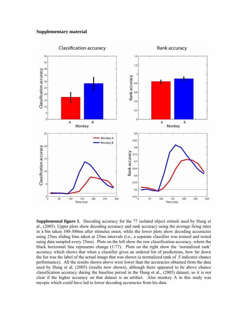
Supplementary material

Supplemental figure 1. Decoding accuracy for the 77 isolated object stimuli used by Hung et al., (2005). Upper plots show decoding accuracy and rank accuracy using the average firing rates in a bin taken 100-300ms after stimulus onset, while the lower plots show decoding accuracies using 25ms sliding bins taken at 25ms intervals (i.e., a separate classifier was trained and tested using data sampled every 25ms). Plots on the left show the raw classification accuracy, where the black horizontal line represents change (1/77). Plots on the right show the ‘normalized rank’ accuracy which shows that when a classifier gives an ordered list of predictions, how far down the list was the label of the actual image that was shown (a normalized rank of .5 indicates chance performance). All the results shown above were lower than the accuracies obtained from the data used by Hung et al. (2005) (results now shown), although there appeared to be above chance classification accuracy during the baseline period in the Hung et al., (2005) dataset, so it is not clear if the higher accuracy on that dataset is an artifact. Also monkey A in this study was myopic which could have led to lower decoding accuracies from his data.

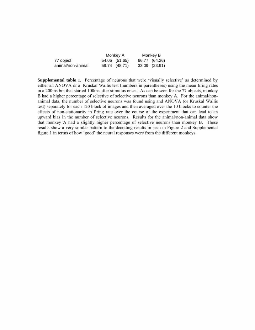
Monkey A Monkey B 77 object 54.05 (51.65) 66.77 (64.26) animal/non-animal 59.74 (48.71) 33.09 (23.91)

Supplemental table 1. Percentage of neurons that were ‘visually selective’ as determined by either an ANOVA or a Kruskal Wallis test (numbers in parentheses) using the mean firing rates in a 200ms bin that started 100ms after stimulus onset. As can be seen for the 77 objects, monkey B had a higher percentage of selective of selective neurons than monkey A. For the animal/non-animal data, the number of selective neurons was found using and ANOVA (or Kruskal Wallis test) separately for each 120 block of images and then averaged over the 10 blocks to counter the effects of non-stationarity in firing rate over the course of the experiment that can lead to an upward bias in the number of selective neurons. Results for the animal/non-animal data show that monkey A had a slightly higher percentage of selective neurons than monkey B. These results show a very similar pattern to the decoding results in seen in Figure 2 and Supplemental figure 1 in terms of how ‘good’ the neural responses were from the different monkeys.

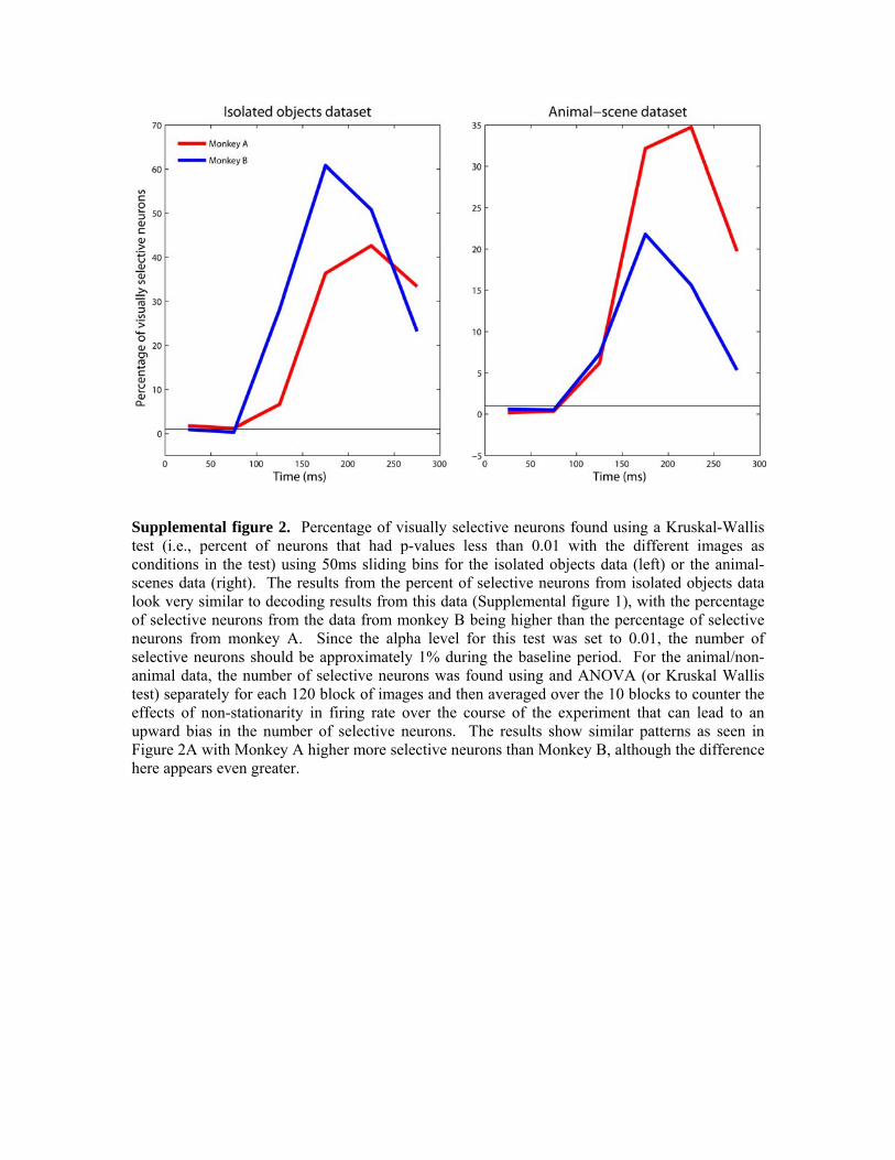
Supplemental figure 2. Percentage of visually selective neurons found using a Kruskal-Wallis test (i.e., percent of neurons that had p-values less than 0.01 with the different images as conditions in the test) using 50ms sliding bins for the isolated objects data (left) or the animal-scenes data (right). The results from the percent of selective neurons from isolated objects data look very similar to decoding results from this data (Supplemental figure 1), with the percentage of selective neurons from the data from monkey B being higher than the percentage of selective neurons from monkey A. Since the alpha level for this test was set to 0.01, the number of selective neurons should be approximately 1% during the baseline period. For the animal/non-animal data, the number of selective neurons was found using and ANOVA (or Kruskal Wallis test) separately for each 120 block of images and then averaged over the 10 blocks to counter the effects of non-stationarity in firing rate over the course of the experiment that can lead to an upward bias in the number of selective neurons. The results show similar patterns as seen in Figure 2A with Monkey A higher more selective neurons than Monkey B, although the difference here appears even greater.

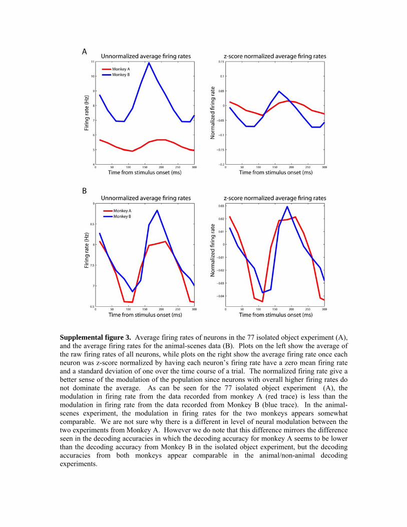
Supplemental figure 3. Average firing rates of neurons in the 77 isolated object experiment (A), and the average firing rates for the animal-scenes data (B). Plots on the left show the average of the raw firing rates of all neurons, while plots on the right show the average firing rate once each neuron was z-score normalized by having each neuron’s firing rate have a zero mean firing rate and a standard deviation of one over the time course of a trial. The normalized firing rate give a better sense of the modulation of the population since neurons with overall higher firing rates do not dominate the average. As can be seen for the 77 isolated object experiment (A), the modulation in firing rate from the data recorded from monkey A (red trace) is less than the modulation in firing rate from the data recorded from Monkey B (blue trace). In the animal-scenes experiment, the modulation in firing rates for the two monkeys appears somewhat comparable. We are not sure why there is a different in level of neural modulation between the two experiments from Monkey A. However we do note that this difference mirrors the difference seen in the decoding accuracies in which the decoding accuracy for monkey A seems to be lower than the decoding accuracy from Monkey B in the isolated object experiment, but the decoding accuracies from both monkeys appear comparable in the animal/non-animal decoding experiments.

77 isolated objects Animal/non-animal Median CV Max time Min time Max time Monkey A 112 162 112 187 Monkey B 87 137 112 162

Supplemental table 2. The bin that had the minimum and maximum firing rate taken from Supplemental figure 2. Values were based on the average firing rates over all neurons using 25ms bins sampled every 25ms (values in parenthesis are given for the normalized average firing rate when they differ from the raw firing rate min or max).

sep ID ave p-val over all ID p-val Monkey A 1.47 (A, B), p = .13 1.42 (A, B), p = .23 Monkey B 1.36 (B, H), p < 10-7 1.36 (B, H), p < 10-3

Supplemental table 3. Median coefficient of variation (CV = stdev/mean) values from the population of neurons from monkey A, and B using the 77 isolated objects data. For each neuron, the coefficient of variation was calculated either separately for each stimulus shown and then averaged together (sep ID ave), or calculated over trials regardless of the stimulus shown (over all ID). The median values over all the neurons are shown above. P-values using a Mann-Whitney U (which is the same as the Wilcoxon rank-sum) were calculated on the CV values for all pairs monkeys. Results from monkey H (recorded by Hung et al., 2005) had less variability compared to monkey A, and B (data not shown), which could partially account for the higher decoding accuracy seen in that monkey.

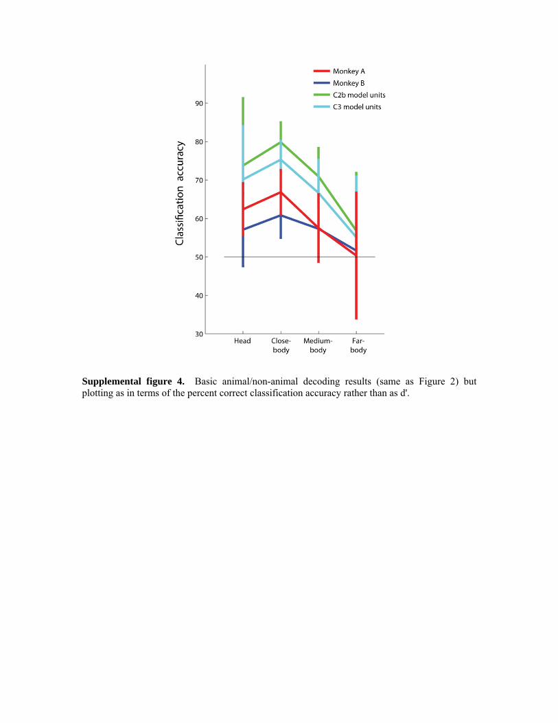
Supplemental figure 4. Basic animal/non-animal decoding results (same as Figure 2) but plotting as in terms of the percent correct classification accuracy rather than as d'.

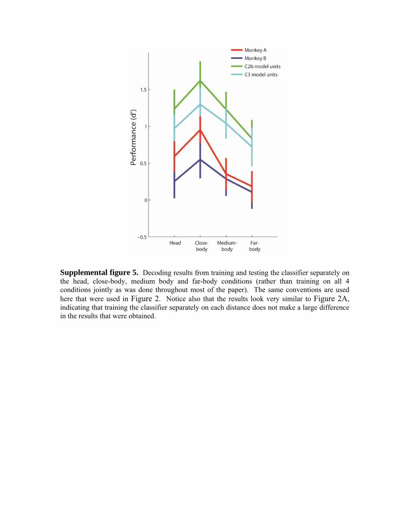
Supplemental figure 5. Decoding results from training and testing the classifier separately on the head, close-body, medium body and far-body conditions (rather than training on all 4 conditions jointly as was done throughout most of the paper). The same conventions are used here that were used in Figure 2. Notice also that the results look very similar to Figure 2A, indicating that training the classifier separately on each distance does not make a large difference in the results that were obtained.

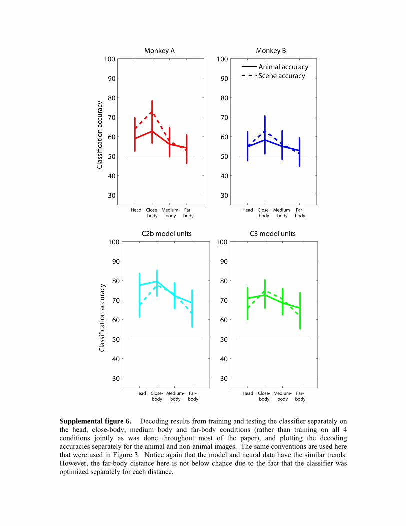
Supplemental figure 6. Decoding results from training and testing the classifier separately on the head, close-body, medium body and far-body conditions (rather than training on all 4 conditions jointly as was done throughout most of the paper), and plotting the decoding accuracies separately for the animal and non-animal images. The same conventions are used here that were used in Figure 3. Notice again that the model and neural data have the similar trends. However, the far-body distance here is not below chance due to the fact that the classifier was optimized separately for each distance.

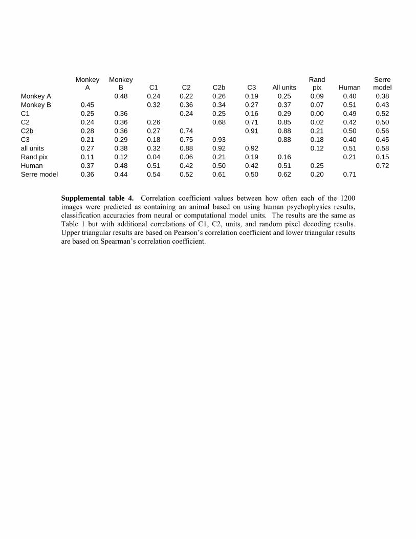
Monkey A

Monkey B C1 C2 C2b C3 All units

Rand pix Human

Serre model

Monkey A 0.48 0.24 0.22 0.26 0.19 0.25 0.09 0.40 0.38 Monkey B 0.45 0.32 0.36 0.34 0.27 0.37 0.07 0.51 0.43 C1 0.25 0.36 0.24 0.25 0.16 0.29 0.00 0.49 0.52 C2 0.24 0.36 0.26 0.68 0.71 0.85 0.02 0.42 0.50 C2b 0.28 0.36 0.27 0.74 0.91 0.88 0.21 0.50 0.56 C3 0.21 0.29 0.18 0.75 0.93 0.88 0.18 0.40 0.45 all units 0.27 0.38 0.32 0.88 0.92 0.92 0.12 0.51 0.58 Rand pix 0.11 0.12 0.04 0.06 0.21 0.19 0.16 0.21 0.15 Human 0.37 0.48 0.51 0.42 0.50 0.42 0.51 0.25 0.72 Serre model 0.36 0.44 0.54 0.52 0.61 0.50 0.62 0.20 0.71

Supplemental table 4. Correlation coefficient values between how often each of the 1200 images were predicted as containing an animal based on using human psychophysics results, classification accuracies from neural or computational model units. The results are the same as Table 1 but with additional correlations of C1, C2, units, and random pixel decoding results. Upper triangular results are based on Pearson’s correlation coefficient and lower triangular results are based on Spearman’s correlation coefficient.

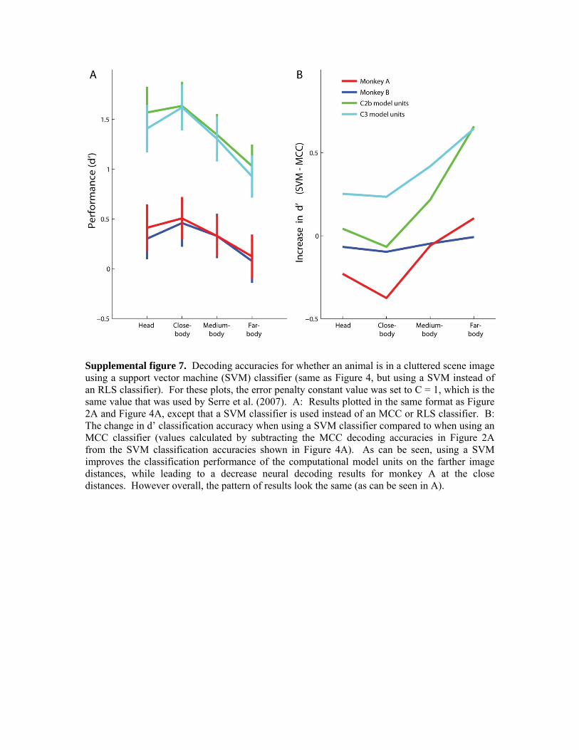
Supplemental figure 7. Decoding accuracies for whether an animal is in a cluttered scene image using a support vector machine (SVM) classifier (same as Figure 4, but using a SVM instead of an RLS classifier). For these plots, the error penalty constant value was set to C = 1, which is the same value that was used by Serre et al. (2007). A: Results plotted in the same format as Figure 2A and Figure 4A, except that a SVM classifier is used instead of an MCC or RLS classifier. B: The change in d’ classification accuracy when using a SVM classifier compared to when using an MCC classifier (values calculated by subtracting the MCC decoding accuracies in Figure 2A from the SVM classification accuracies shown in Figure 4A). As can be seen, using a SVM improves the classification performance of the computational model units on the farther image distances, while leading to a decrease neural decoding results for monkey A at the close distances. However overall, the pattern of results look the same (as can be seen in A).

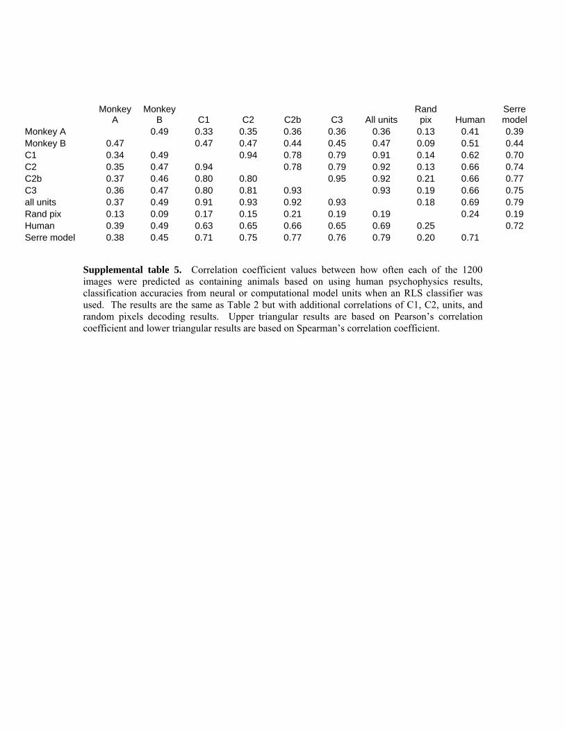
Monkey A

Monkey B C1 C2 C2b C3 All units

Rand pix Human

Serre model

Monkey A 0.49 0.33 0.35 0.36 0.36 0.36 0.13 0.41 0.39 Monkey B 0.47 0.47 0.47 0.44 0.45 0.47 0.09 0.51 0.44 C1 0.34 0.49 0.94 0.78 0.79 0.91 0.14 0.62 0.70 C2 0.35 0.47 0.94 0.78 0.79 0.92 0.13 0.66 0.74 C2b 0.37 0.46 0.80 0.80 0.95 0.92 0.21 0.66 0.77 C3 0.36 0.47 0.80 0.81 0.93 0.93 0.19 0.66 0.75 all units 0.37 0.49 0.91 0.93 0.92 0.93 0.18 0.69 0.79 Rand pix 0.13 0.09 0.17 0.15 0.21 0.19 0.19 0.24 0.19 Human 0.39 0.49 0.63 0.65 0.66 0.65 0.69 0.25 0.72 Serre model 0.38 0.45 0.71 0.75 0.77 0.76 0.79 0.20 0.71

Supplemental table 5. Correlation coefficient values between how often each of the 1200 images were predicted as containing animals based on using human psychophysics results, classification accuracies from neural or computational model units when an RLS classifier was used. The results are the same as Table 2 but with additional correlations of C1, C2, units, and random pixels decoding results. Upper triangular results are based on Pearson’s correlation coefficient and lower triangular results are based on Spearman’s correlation coefficient.

Supplemental figure 8. SVM animal/non-animal decoding results as a function of the error penalty parameter (C), plotting separately for the head, close-body, medium-body and far-body conditions. As can be seen, the best regularization constant value is around 0.001 for most image distances and model unit conditions. For the close-body condition at the peak error penalty constant value there is not much difference in the decoding results between using C1 and model units of all types. For the other conditions, generally there is a slight advantage to using all unit types and using more units (although this advantage tends to be smaller around the optimal error penalty constant value, than when compared to the default error penalty constant value C=1 that was used by Serre et al. (2007)). Also shown on the right of each plot are the decoding RLS results (same as Figure 6B) that were found by optimizing the error penalty constant using only the training data.

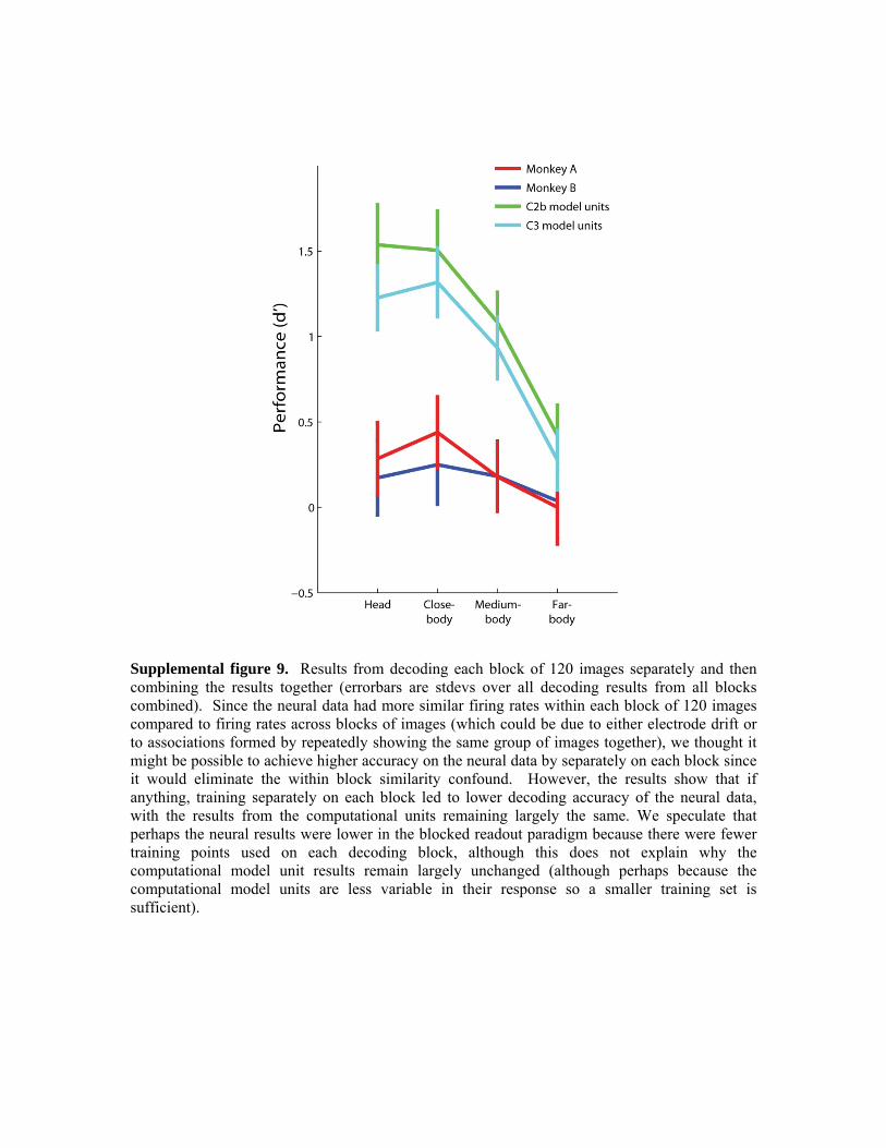
Supplemental figure 9. Results from decoding each block of 120 images separately and then combining the results together (errorbars are stdevs over all decoding results from all blocks combined). Since the neural data had more similar firing rates within each block of 120 images compared to firing rates across blocks of images (which could be due to either electrode drift or to associations formed by repeatedly showing the same group of images together), we thought it might be possible to achieve higher accuracy on the neural data by separately on each block since it would eliminate the within block similarity confound. However, the results show that if anything, training separately on each block led to lower decoding accuracy of the neural data, with the results from the computational units remaining largely the same. We speculate that perhaps the neural results were lower in the blocked readout paradigm because there were fewer training points used on each decoding block, although this does not explain why the computational model unit results remain largely unchanged (although perhaps because the computational model units are less variable in their response so a smaller training set is sufficient).

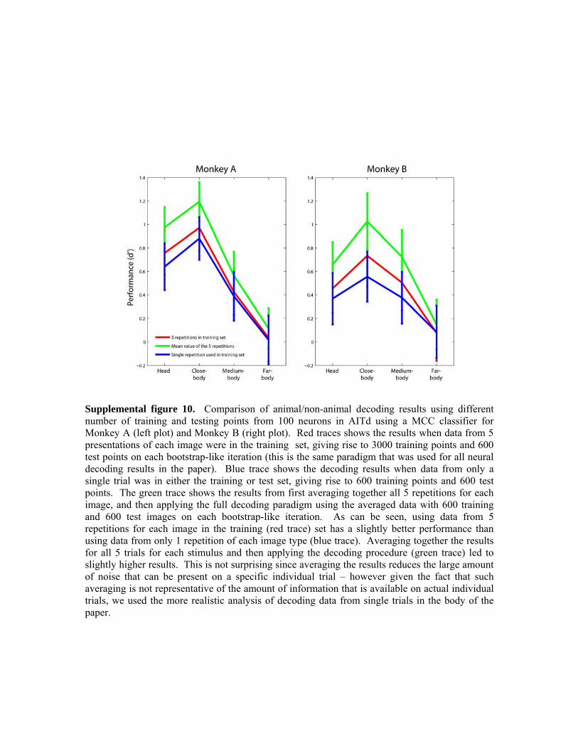
Supplemental figure 10. Comparison of animal/non-animal decoding results using different number of training and testing points from 100 neurons in AITd using a MCC classifier for Monkey A (left plot) and Monkey B (right plot). Red traces shows the results when data from 5 presentations of each image were in the training set, giving rise to 3000 training points and 600 test points on each bootstrap-like iteration (this is the same paradigm that was used for all neural decoding results in the paper). Blue trace shows the decoding results when data from only a single trial was in either the training or test set, giving rise to 600 training points and 600 test points. The green trace shows the results from first averaging together all 5 repetitions for each image, and then applying the full decoding paradigm using the averaged data with 600 training and 600 test images on each bootstrap-like iteration. As can be seen, using data from 5 repetitions for each image in the training (red trace) set has a slightly better performance than using data from only 1 repetition of each image type (blue trace). Averaging together the results for all 5 trials for each stimulus and then applying the decoding procedure (green trace) led to slightly higher results. This is not surprising since averaging the results reduces the large amount of noise that can be present on a specific individual trial – however given the fact that such averaging is not representative of the amount of information that is available on actual individual trials, we used the more realistic analysis of decoding data from single trials in the body of the paper.

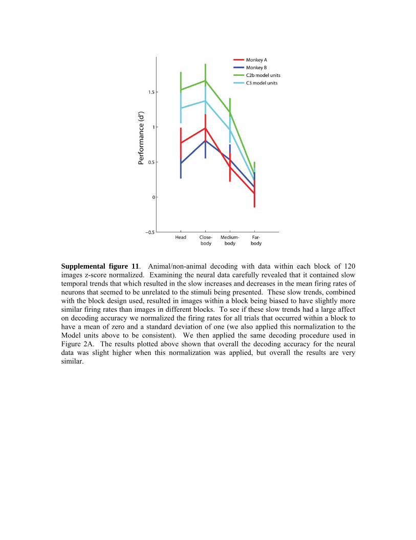
Supplemental figure 11. Animal/non-animal decoding with data within each block of 120 images z-score normalized. Examining the neural data carefully revealed that it contained slow temporal trends that which resulted in the slow increases and decreases in the mean firing rates of neurons that seemed to be unrelated to the stimuli being presented. These slow trends, combined with the block design used, resulted in images within a block being biased to have slightly more similar firing rates than images in different blocks. To see if these slow trends had a large affect on decoding accuracy we normalized the firing rates for all trials that occurred within a block to have a mean of zero and a standard deviation of one (we also applied this normalization to the Model units above to be consistent). We then applied the same decoding procedure used in Figure 2A. The results plotted above shown that overall the decoding accuracy for the neural data was slight higher when this normalization was applied, but overall the results are very similar.

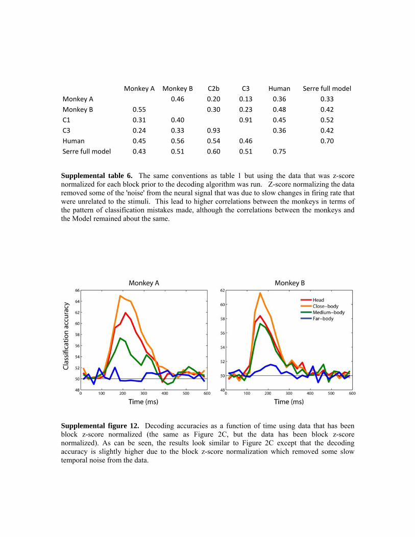
Monkey A  Monkey B  C2b  C3  Human  Serre full model Monkey A  0.46  0.20  0.13  0.36  0.33 Monkey B  0.55  0.30  0.23  0.48  0.42 C1  0.31  0.40  0.91  0.45  0.52 C3  0.24  0.33  0.93  0.36  0.42 Human  0.45  0.56  0.54  0.46  0.70 Serre full model  0.43  0.51  0.60  0.51  0.75 

Supplemental table 6. The same conventions as table 1 but using the data that was z-score normalized for each block prior to the decoding algorithm was run. Z-score normalizing the data removed some of the 'noise' from the neural signal that was due to slow changes in firing rate that were unrelated to the stimuli. This lead to higher correlations between the monkeys in terms of the pattern of classification mistakes made, although the correlations between the monkeys and the Model remained about the same.

Supplemental figure 12. Decoding accuracies as a function of time using data that has been block z-score normalized (the same as Figure 2C, but the data has been block z-score normalized). As can be seen, the results look similar to Figure 2C except that the decoding accuracy is slightly higher due to the block z-score normalization which removed some slow temporal noise from the data.

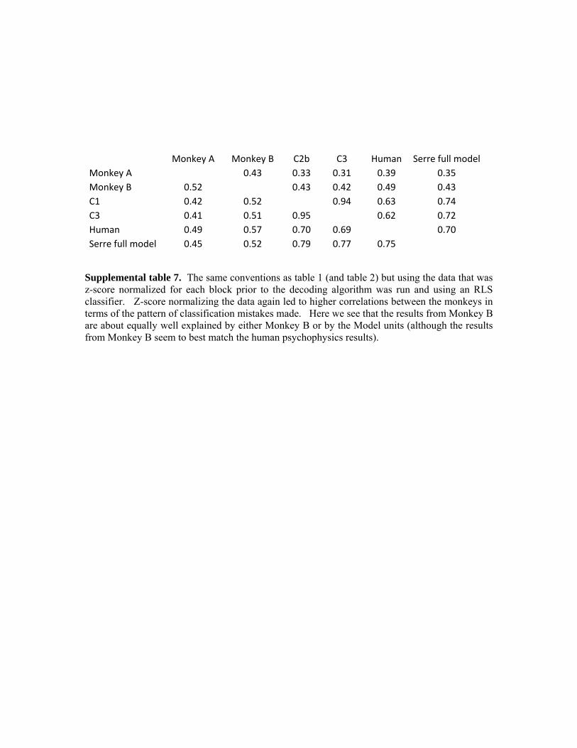
Monkey A  Monkey B  C2b  C3  Human  Serre full model Monkey A  0.43  0.33  0.31  0.39  0.35 Monkey B  0.52  0.43  0.42  0.49  0.43 C1  0.42  0.52  0.94  0.63  0.74 C3  0.41  0.51  0.95  0.62  0.72 Human  0.49  0.57  0.70  0.69  0.70 Serre full model  0.45  0.52  0.79  0.77  0.75 

Supplemental table 7. The same conventions as table 1 (and table 2) but using the data that was z-score normalized for each block prior to the decoding algorithm was run and using an RLS classifier. Z-score normalizing the data again led to higher correlations between the monkeys in terms of the pattern of classification mistakes made. Here we see that the results from Monkey B are about equally well explained by either Monkey B or by the Model units (although the results from Monkey B seem to best match the human psychophysics results).