Examination of Some Heavy Metal Pollution in Roadside ...

University of Łódź

Chair of Modelling Teaching Processes

A Doctoral Dissertation of

Punsiri Dam-o

Examination of Some Heavy Metal Pollution

in Roadside Plants

Using X-Ray Spectroscopy

Supervisor – prof. dr hab. Tadeusz Wibig

Łódź, November 2015.

i

CONTENTS

CONTENTS i

LIST OF FIGURES vii

LIST OF TABLES xiii

1 INTRODUCTION 1

1.1 Origin of the idea 1

1.2 Importance 3

1.2.1 Physical point of view 3

1.2.2 Educational point of view 5

1.3 Objectives 7

2 REVIEW OF THE RESULTS EXISTING IN THE LITERATURE 9

2.1 Origin of heavy metal pollutants on roadside 9

2.1.1 Vehicular emissions: exhaust 9

2.1.2 Vehicular emissions: non-exhaust 10

2.1.3 Road construction 11

2.1.4 Other sources 11

2.2 Automotive heavy metal pollution on the roadside 12

2.2.1 The prior studies related to the distribution of heavy metal pollutants

aside the roads

12

ii

2.2.2 Other studies related to the heavy metal pollution on roadside 16

2.3 Plant samples from roadside as indicator of heavy metal pollution on the

roadside

19

2.3.1 Dandelion (Taraxacum officinale F.H. Wigg.) 19

2.3.2 Yarrow (Achillea millefolium L.) 20

2.3.3 Siam weed (Chromolaena odorata (L.) King & Robinson) 21

2.3.4 Tridax daisy (Tridax procumbens L.) 23

3 METHOD 26

3.1 Samples 26

3.1.1 Plant species 26

3.1.2 Sampling strategy 27

3.1.3 Sample preparation 28

3.2 X-ray spectrometer 29

3.3 X-ray spectrum analysis software 31

3.3.1 Comparison of the best fit of the Gaussian function to X-ray

fluorescence peaks using the Gaussian-fit (by trained and untrained

personnel) and SPECTRA programs

33

3.3.2 The fitting procedure of the Gaussian-fit and SPECTRA programs 37

3.4 Heavy metal elements to be examined 44

4 INVOLVEMENT OF SCHOOL STUDENTS IN THE RESEARCH 45

4.1 Nonprofessional scientists in a real scientific research 45

iii

4.2 Why children (school students) are expected to follow the proposition of the

research project?

47

4.3 Organization of the “nuclear e-cology” project 49

4.3.1 Biology and environmental science team 49

4.3.2 X-ray spectrometry laboratory team 50

4.3.3 General physics team 50

4.4 Interest for the physics teachers 51

4.5 Activities for the school students 52

4.6 Learning materials 55

4.6.1 The “nuclear e-cology” website 55

4.6.2 Tutorial video clips and documents 57

4.7 Project achievement 58

4.7.1 Participants of the project 58

4.7.2 Communication between the laboratory scientists and the

participants

60

4.7.3 Experimental reports of the groups 63

4.8 Opinions from school teachers 65

5 RESULTS AND DISCUSSION 66

5.1 The studied sites 66

5.2 Estimation of the accuracies of observing results 68

5.3 Average relative abundances of the heavy metal elements in the roadside

plants: comparison among different studied sites

71

iv

5.3.1 Average relative abundance of iron 71

5.3.2 Average relative abundance of nickel 73

5.3.3 Average relative abundance of zinc 76

5.3.4 Average relative abundance of lead 78

5.3.5 Average relative abundances of bromine, rubidium and strontium 80

5.4 Distribution of the heavy metals with respect to the distance of the road axis 86

5.4.1 The studied site G7 (Wartkowice, Poland) 86

5.4.2 The final analysis of all collected data 89

5.4.3 Comparison of the average characteristic decrease length of iron

with other results

92

5.4.4 Comparison of the average characteristic decrease length of nickel

with other results

93

5.4.5 Comparison of the average characteristic decrease length of zinc

with other results

94

5.4.6 Comparison of the average characteristic decrease length of lead

with other results

95

5.4.7 Comparison of the average characteristic decrease length of bromine

with other results

97

5.4.8 Summary of the average characteristic decrease length of the heavy

metal pollution

98

6 CONCLUSION REMARKS 99

v

7 POSSIBILITY TO CONTINUE THE RESEARCH 100

8 SUMMARY 102

APPENDIX A LEARNING MATERIALS AND ACTIVITIES FOR THE

PARTICIPANTS OF THE “NUCLEAR E-COLOGY” PROJECT

104

A.1 Video instruction 104

A.2 The “nuclear e-cology” webpage 109

A.3 Facebook page of the project 114

A.4 List of the participants 116

A.5 Exercise of the Gaussian best fit 117

A.6 An example of the group report 119

A.7 Examples of conversation during the teleconference sessions 125

APPENDIX B RESULTS 127

B.1 Distribution of the heavy metals with respect to the distance of the road axis

of the studied site G6, G16, G18, G34, G27 and G28

127

B.1.1 The studied site G6 (Rawa Mazowiecka I, Poland) 127

B.1.2 The studied site G16 (Rawa Mazowiecka II, Poland) 130

B.1.3 The studied site G18 (Łowicz, Poland) 132

B.1.4 The studied site G34 (Łódź, Poland) 135

B.1.5 The studied site G27 (Nakhon Si Thammarat I, Thailand) 137

B.1.6 The studied site G28 (Nakhon Si Thammarat II, Thailand) 140

vi

B.2 Dispersion of relative abundances of heavy metal elements in the roadside

plants of the studied sites in Thailand

143

LITERATURE CITED 145

ACKNOWLEDGEMENTS 154

BIOGRAPHY SKETCH 155

vii

LIST OF FIGURES

Figure 1.1 The plants to be studied: dandelion, yarrow, Siam weed and tridax

daisy

7

Figure 2.1 Heavy metal concentrations normalized with respect to copper in

plant samples collected at unpolluted sites.

24

Figure 3.1 Illustration of the sampling strategy with the codes of samples at

particular areas

27

Figure 3.2 A scheme of preparation of plant samples 28

Figure 3.3 The X-ray spectrometer and its working principle 29

Figure 3.4 An X-ray spectrum of a sample of the dandelion 30

Figure 3.5 The Gaussian-fit program shows the scatter plot of an X-ray spectrum

file.

32

Figure 3.6 Examples of X-ray fluorescence peaks of iron and sulphur fit with the

Gaussian curve by a test participant and myself (trained person).

35

Figure 3.7 Examples of the background subtraction of the Gaussian-fit and

SPECTRA programs

39

Figure 3.8 The plots of the net area normalized with respect to gallium of

analyzed elements from two spectra of roadside grass by using the

Gaussian-fit and SPECTRA programs.

41

viii

Figure 3.9 The region where the emission lines of L1 and L 2 of lead and K1

of arsenic are located and the region where the fluorescence peak of

lead is identified.

43

Figure 4.1 A scheme of activities in the experimental lesson for the participants 54

Figure 4.2 Site map of the “nuclear e-cology” webpage 56

Figure 4.3 Example photos from e-mail correspondence, meeting in person and

teleconferences

62

Figure 5.1 Histograms showing the distributions of iron, nickel, zinc, lead,

bromine, rubidium and strontium in the samples of Poland

68

Figure 5.2 The average relative abundance of iron in roadside plants of the

different studied sites

72

Figure 5.3 The average relative abundance of nickel in roadside plants of the


74

Figure 5.4 The average relative abundance of zinc in roadside plants of the


76

Figure 5.5 The average relative abundance of lead in roadside plants of the


78

Figure 5.6 The average relative abundance of bromine in roadside plants of the


81

Figure 5.7 The average relative abundance of rubidium in roadside plants of the


83

Figure 5.8 The average relative abundance of strontium in roadside plants of the


84

ix

Figure 5.9 The studied site G7 87

Figure 5.10 The lateral distribution of heavy metal relative abundances with

respect to copper in the roadside plants from the studied site G7

88

Figure 5.11 The exponential models of the decreasing relative abundances of

heavy metal elements in the samples at the studied site G7

(Wartkowice), G16 (Rawa Mazowiecka), G18 (Łowicz) and G27

(Nakhon Si Thammarat I)

90

Figure 5.12 Combined data from the studied site G7, G16, G18 and G27 where

decreasing relative abundance pattern of the heavy metal elements

can be seen.

91

Figure 5.13 Comparison of the average characteristic decrease length of iron of

the present study to the similar study at the Moscow highways by

Alov et al.

92

Figure 5.14 Comparison of the average characteristic decrease length of nickel of

the present study to the similar studies at USA by Lagerwerff and

Specth and China by Zhao et al.

94

Figure 5.15 Comparison of the average characteristic decrease length of zinc of

the present study to the similar studies at USA by Lagerwerff and

Specth and France by Viard et al.

95

Figure 5.16 Comparison of the average characteristic decrease length of lead of

the present study to the similar studies in USA by Lagerwerff and

Specth, Syria by Othman et al., France by Viard et al. and China by

Zhao et al.

96

x

Figure 5.17 The average characteristic decrease length of bromine from the

present study

97

Figure A.1 A screenshot of the video instruction “how to fit background and

peaks” which shows a demonstration of fitting the background of an

X-ray spectrum.

104

Figure A.2 A screenshot of the video instruction “how to write group report”

which shows the standard report form in an Excel spreadsheet.

105

Figure A.3 A screenshot of the video instruction “research paper” which shows

how to present research results using graphs.

106

Figure A.4 A screenshot of the video instruction concerning “sample preparation

and measurement” which shows the sample treatment for

measurement with the TXRF technique.

107

Figure A.5 Screenshots from the “nuclear e-cology” website of the “news” page

show an access to the experimental results database (from group

reports) and the individual group activity pages.

109

Figure A.6 Screenshots from the “nuclear e-cology” website of the “X-ray”

pages, plant species descriptions and the “software for spectrum

analysis” pages

113

Figure A.7 A screenshot of the Facebook page of the “nuclear e-cology” project

which shows announcements and photos from the updated activities.

114

Figure A.8 An example of the exercise of the Gaussian best fit in the Excel

spreadsheet form

117

xi

Figure A.9 Examples of participants’ answers obtained from the exercise of the

Gaussian best fit.

118

Figure A.10 The first page of the report form for the participants to fill in the

information about their group, the studied site and the results from

fitting the X-ray spectra

119

Figure A.11 The second page of the report form for presenting graphs showing the

distributions of the studied relative abundances of the heavy metal

elements

120

Figure A.12 The third page of the report form for writing the discussion and

conclusion

121

Figure B.1 The studied site G6 128

Figure B.2 The lateral distribution of heavy metal relative abundances with


129




132




134




137


xii



139




142

Figure B.13 Histograms showing the distributions of iron, nickel, zinc, lead,

bromine, rubidium and strontium in the samples of Thailand.

143

xiii

LIST OF TABLES

Table 2.1 Concentrations of heavy metal elements in parts of the dandelion

collected from different regions studied by early research groups.

19

Table 2.2 Concentrations of heavy metal elements in parts of the yarrow

collected from different regions studied by early research groups.

21

Table 2.3 Concentrations of heavy metal elements in parts of the Siam

weed collected from different regions studied by early research

groups.

22

Table 2.4 Concentrations of heavy metal elements in parts of the tridax

daisy collected from different regions studied by early research

groups.

23

Table 3.1 Comparison of the areas under the Gaussian curves from the best

fit of iron and sulphur peaks among the results obtained from a

test participant and myself (trained person) using the Gaussian-fit

and SPECTRA programs.

36

Table 3.2 The comparisons of net areas normalized with respect to gallium

analyzed from two spectra of roadside grass samples using the

Gaussian-fit and SPECTRA programs.

40

Table 4.1 Participants of the 2013/2014 project 58

Table 5.1 List of studied sites and plant samples 66

xiv

Table 5.2 Parameters in Fig 5.1 and the estimation of accuracies of the

relative abundances of the heavy metal elements

70

Table 5.3 Height of the barriers, traffic rates and decreasing parameter r0 at

the studied site G7, G16, G18 and G27

91

Table 5.4 Comparison of the average characteristic decrease length

(parameter r0) of the present study to the experimental results of

the other studies

98

Table A.1 List of the participants who contributed their experimental results

to the present study.

116

1

1 INTRODUCTION

1.1 Origin of the idea

Grazing fields, vegetable farms and residential areas are the common things that I usually see

along the roadside, while traveling on a highway away from the city limits. It seems to me that

they have been located there for a very long time. I used to question myself if there are animals

grazing in the fields, people who are living in those areas or even myself eating vegetables from

those farms, are we safe from highway pollution?

After searching for an answer, I found out that in regards to human health and the environment

that we live in, many groups of scientists had conducted their experiments to measure the

concentrations of heavy metals deposited in dust, soil, plant and animal samples which they took

from the roadside. The experimental results indicated that the heavy metals emitted by the

automobiles from the roads were distributed to the roadside and were accumulated in the

samples. Furthermore, at some sites the concentrations of some heavy metals were higher than

recommended safety limit and potentially caused health problems in both humans and animals.

However, the actual distance away from the roadside of the elemental distribution had never

been documented. At this point, it inspired me to conduct my own research to find out at what

distance different kinds of heavy metal pollution can be deposited on the roadside and in what

quantities?

I then made further searches for a method which could be used for the measurement of

“elemental abundance”. Until late 2012, I was given a chance by the Faculty of Physics and

2

Applied Informatics at the University of Łódź (where I was studying), to visit the physics

laboratory of Kazan Federal University Branch in Zelenodolsk, Russia. During the visit, Mr.

Alexander Dyganov, a physicist of the laboratory, presented to me an X-ray spectrometer which

was used by the university students in studying the typical X-ray spectrum from different types

of materials. A special advantage of this spectrometer was that the students were able to perform

an experiment remotely via the Internet. Unfortunately, it was out of use for a few years because

one out of the two detectors was broken. It seemed that the X-ray spectrometer had been left

behind in that laboratory.

I told this story to my colleagues in the “Physics Remote Laboratories for Education” research

group of the Chair of Modelling Teaching Processes, Faculty of Physics and Applied

Informatics, University of Łódź. We got an idea to fix the broken detector and to adapt the

spectrometer for a more attractive experiment. Then a research related to X-ray spectroscopy

application for environmental study was proposed and everyone agreed. At that moment the

research topic on the examination of heavy metals in environmental samples was developed.

Concerning the broken X-ray detector in Kazan Federal University Branch in Zelenodolsk,

unfortunately, we found that it could not be repaired. The spectrometer itself was assembled

using old technology many years ago.

In 2013, the “nuclear e-cology” project was established in coorperation of three research teams:

the general physics team from University of Łódź (including myself), the biology and

environmental science team from University of Wrocław and the X-ray spectrometry laboratory

team from Jan Kochanowski University in Kielce. The project involved the modern physics in

the studies of the ecological system. In the first research subject we decided to examine some

heavy metal pollution in the roadside plants using the X-ray spectroscopy.

3

1.2 Importance

The importance of this research concerns two points of view: physical and educational.

1.2.1 Physical point of view

Road transportation activity, a primal component of economic development and human welfare,

is increasing around the world as the economies grow. Road traffic has been highlighted as a

major source of heavy metal emissions (e.g., cadmium, copper, iron, lead, zinc and nickel).

Consequently, the rise of the road transportation activity causes the higher levels of emitted

metals, which impact the ecological environment on the roadside and the surrounding areas such

as farmlands, pastures, rivers and residences. The heavy metals may enter the food chain as a

result of contaminating edible plants or their intake by people. If these levels are excessive, the

metals can cause serious health risks. For example:

zinc, in fact, is an essential trace element and serves a number of roles and functions in

the human body (e.g., being a component of enzymes involved in the synthesis and

metabolism of carbohydrates, lipids, proteins, nucleic acids and other micro-nutrients;

involving in DNA synthesis and the process of genetic expression; stabilizing cellular

components and membraned). However, the prolonged intake of more than 300 mg per

day of zinc (Fosmire, 1990) can lead to disturbance of copper metabolism, causing low

copper status, reduced iron function, impaired immune function; can cause abdominal

pain, nausea, vomiting, diarrhoea, epigastric pain, lethargy and fatigue;

lead is a cumulative toxicant. However there is no known level of lead exposure that is

considered safe for humans. Once it enters the body, it is distributed to the brain, kidneys,

4

liver and bones. The body stores lead in the teeth and bones where it accumulates over

time. Lead affects the development of the brain and nervous system in young children and

causes high blood pressure and kidney damage in adults. Moreover, the exposure of

pregnant women to high levels of lead can cause miscarriage, stillbirth, premature birth,

low birth weight and other minor malformations;

bromine would cause different effects depending on the chemical compounds. In case

of 1,2-dibromoethane (Gift et al., 2004), which was used as an anti-knock additive in lead

fuels, potentially causes adverse reproductive and fertility effects.

The heavy metals have non-biodegradable characteristics. They can remain in the roadside

environment including the food chain for a very long period of time. It is important to know

how the heavy metals are distributed on the roadside. This will suggest us how to protect our

health from the heavy metal pollution.

In the early works, some research groups conducted the experiments to examine the

concentration of heavy metal elements in roadside samples within different distances from the

road. For example:

in the year 1970, the scientists at the Air Pollution Research Center, in Califonia, USA

(Schuck and Locke, 1970) examined lead in cauliflower collected from the distances of

15 – 360 m from a highway. They found the presence of a detectable amount of lead when

the cauliflower was grown within 135 m of the highway;

in the late 20th century, the scientists at the Department of Radiation Protection and

Nuclear Safety, Atomic Energy Commission of Syria (Othman et al., 1997) studied lead

levels in roadside soils, vegetables and plants in the city of Damascus, Syria. They found

5

the relationship between lead concentration in the samples and the distance within 80 m

from the road edge;

in the early 21st century, the scientists at the Department of Analytical Chemistry in

Moscow, Russia (Alov et al., 2001) investigated the iron, manganese, titanium and lead

content distribution in soil in vicinity of the Moscow highway. They found out that these

elemental pollutions are observed aside the highway up to 100 – 200 m;

three years later, the scientists at the Laboratoire BFE – Equipe PEE, in France (Viard

et al., 2004) measured the concentrations of lead, zinc and cadmium in soil, grass and

snails within 320 m from a highway. They found that the highway induces a contamination

up to all the distances they studied.

Detailed analysis which is to be shown in chapter 2 presents that different research groups

obtained different results, even as regards the same heavy metal element such as lead. The

question “how the heavy metal elements can really be deposited aside the roadside” is still an

open one. We then decided to conduct the research to learn about the distribution – in general

case, of heavy metal pollution on the roadside.

1.2.2 Educational point of view

The importance of the research in general is also the education of the next generations. Nations

address in principle the high priority in physics through science, technology and education

policies by providing infrastructure and funding. People trained in physics are essential for

continuing research in a particular field, and for maintaining a technically sophisticated

6

workforce. Physics worldwide has a long tradition of producing scientists in different fields and

ranges of education.

On the level of graduate education, students dealing with experimental and theoretical physics

have an opportunity to experience and solve complex problems. Their trainings involve design,

build, and test of instrumentations. Additionally, they learn teamwork, management, and

communication skills in addition to gain new technical knowledge and expertise. Their skills

are readily applied to a wide range of technological problems in their homelands; in medicine,

industry, environment, business, management, and government. Future physical knowledge and

technology will be directed by these people. Undergraduate’s degree in physics provides a

foundation for graduate study in physics. The undergraduate students should have an

opportunity to acquire deep conceptual understanding of fundamental physics and gain

important skills for experimentations in physics.

Young students are usually fascinated by natural phenomena. A way to attract them to the

educational path in physics is to reinforce them early and maintain their interest. Healthy

curiosity has the power of inspiring students in the educational process. On the other hand people

wish to have a good quality of life. Physical health and emotional well-being connect people to

the environment in which they live. People can create a good environment by the assistance of

efficient technologies. The technologies could not be developed without the knowledge of

science (physics).

We understand the significance of physics and education linked to environmental science. We

therefore established the project which dedicates school students of worldwide countries with

the experimental lessons in physics on environmental investigation. We wish to prepare the

young people to become the next generation of scientists (physicists).

7

1.3 Objectives

The objectives of the research are to study the distribution of heavy metal pollution on roadside

taking into consideration the following aspects:

1) characteristic length of the distribution of deposited heavy metal elements;

2) average relative abundance of the heavy metal elements on the studied sites.

The heavy metal elements of interest are iron, nickel, zinc, lead, bromine, rubidium and

strontium. We studied plant species growing in vicinity of the road in Poland and Thailand (Fig.

1.1):

in Poland: leaves of Taraxacum officinale F. H. Wigg. (dandelion) or Achillea

millefolium L. (yarrow);

in Thailand: leaves of Chromolaena odorata (L.) King & Robinson (Siam weed) or

Tridax procumbens L. (tridax daisy).

(a) (b)

Figure 1.1 The plants to be studied (a) dandelion, (b) yarrow, (c) Siam weed (Medicinal herbs,

n. d.) and (d) tridax daisy

8

(c) (d)

Figure 1.1 (Continue)

9

2 REVIEW OF THE RESULTS EXISTING

IN THE LITERATURE

2.1 Origin of heavy metal pollutants on roadside

After the first modern highway was constructed, motor vehicles and their usage developed very

rapidly. This resulted in transportation becoming the major cause of pollution, especially in

urban areas. The pollution from vehicles has been linked to effecting people’s health

(Krzyzanowski et al., 2005) and also causing ecological problems (Bolin et al., 1986). The

scientists address their concerns on road pollution via “scientific research”, in order to

observe/monitor the pollution and to understand and control the problems. This is presented

extensively in various literatures, for example, the “Contamination of Roadside Soil and

Vegetation with Cadmium, Nickel, Lead, and Zinc” (Lagerwerff and Specht, 1970), the

“Highway Pollution” (Hamilton and Harrison, 1991), the “Automobiles and Pollution”

(Degobert, 1992). The ongoing study on road pollution will never be out-of-date. The demand

of the vehicle usage throughout the world has not decreased since 1960 (Ribeiro et al., 2007).

2.1.1 Vehicular emissions: exhaust

Lead pollution has traditionally been regarded, due to the exhaust from the gasoline combustion

engine into the atmosphere. Before the use of leaded gasoline became prohibited, lead in the

chemical form of tetraethyl lead was added to an anti-knocking agent (Jungers et al., 1975). The

highest consumption of leaded gasoline was noted in early 1970’s before being phased-out for

10

good (Nriagu, 1990). Even though the use of lead has been banned in gasoline for decades, lead

particulate pollution from automotive emissions has been investigated in recent years (e.g.,

Lammel et al., 2002; Grigalaviciene et al., 2005; Szynkowska et al., 2009; Zhang et al., 2012;

Zakir et al., 2014) due to its toxicity and persistence characteristics. At present the emissions of

gasoline, diesel and biodiesel vehicles, the lead can be detected in trace level which is lower

than the levels of manganese, iron, nickel, copper and zinc (Cheung et al., 2010).

2.1.2 Vehicular emissions: non-exhaust

Abrasive processes of brake linings, tires, and general vehicle wears over time contribute in

emitting different kinds of metal pollutants onto the roadside. Brake linings are composed of a

high content of iron and copper. During the application of the brakes, friction and heat result in

the high emissions of iron and copper (Luhana et al., 2004). In vulcanization, zinc is one of the

main additives used, therefore the corrosion of tires can result in the high emission of zinc

(Hjortenkrans et al., 2007). Besides the metallic compositions of brake linings and tires, the

other factors such as the size of vehicles, acceleration of vehicles and road surface can also

affect the content of metal emissions. The major parts of vehicles, skeleton and body panels are

composed of iron (steel) and aluminum, respectively. Their erosions result in iron and aluminum

emissions. Parts of iron, copper, zinc, aluminum and other metals, for example, manganese,

nickel, titanium, lead, bromine, cadmium and molybdenum are also found as the non-exhaust

emissions.

11

2.1.3 Road construction

Iron are largely use in road construction (Lagerwerff and Specht, 1970; Skinner, 2008) as well

as in components of bridges, concrete paves and barriers. Welding work and corrosion of the

iron parts lead to the emission of the iron into the environment. Also rock and soil brought in

from elsewhere for the construction of a new road, can in some cases contain a higher metal

composition than the original. This activity may be considered on its responsibility to metal

pollution on roadside as well (Ward et al., 1977).

2.1.4 Other sources

Metal pollution on roadside and its vicinity could be found in considerable levels in industrial,

power plant, mining and agricultural areas. For example, higher than critical limits of cadmium,

lead and zinc were found in the areas of mining and smelting industry of Upper Silesia, South

Poland (Dudka et al., 1995). Other examples of this is when arsenic on a concentration level

exceeding the World Health Organization (WHO) was found in surface drainage and

groundwater in the tin mining area in Ron Phibun district, Nakhon Si Thammarat province,

Thailand (Williams et al., 1996). The increases of cadmium, lead, and arsenic concentrations

due to the use of fertilizer and pesticide were also observed in agricultural areas of Kermanshah

province, Iran (Atafar et al., 2010). In addition, the other activities of humans such as the

dumping of waste and nuclear detonations may also effect the contamination of heavy metals

on roadside.

12

2.2 Automotive heavy metal pollution on the roadside

The automotive heavy metal pollution has been the subject of many investigations. These have

included studies of the heavy metal pollution associated with the ecological system (air, soils,

plants and animals) in vicinity of the roads.

2.2.1 The prior studies related to the distribution of heavy metal pollutants aside

the roads

In early 1970, the Air Pollution Research Center, in California, USA (Schuck and Locke, 1970)

reported the study about the relationship of lead content with certain consumer crops:

cauliflower, tomato, cabbage, strawberry and Valencia orange. The samples were collected at

different distances within 15 – 360 m in the vicinity of a highway with the traffic rate of 58,000

units per day. In this study, the colorimetric dithizone technique was used for sample analysis.

The clearest evidence results came from the examination of the unwashed cauliflower and

tomato crops. The analysis indicated the presence of detectable lead when the cauliflower and

tomato crops were grown within 200 and 360 m of the highway, respectively. The concentration

of lead in the crops dropped rapidly within a hundred meter of the highway. The relationship

between lead concentration and the distance was described by the exponential function.

In the middle of 1970, the U. S. Soils Laboratory, USA (Lagerwerff and Specth, 1970) published

a research paper about cadmium, nickel, lead and zinc pollution in roadside soil and grass. The

samples were collected at different distances within 8 – 32 m at the areas adjacent to four roads

of West of U. S. 1 at Beltsville and Washington-Baltimore Parkway at Bladensburg in Madison,

Wisconsin state, Interstate 29 at Platte City in Missouri, north of Kansas City and Seymour Road

13

in the northern section of the Cincinnati metropolitan area. The traffic rates per day of the roads

were 7,500 – 48,000 units. The samples were analyzed using atomic absorption spectroscopy.

The analysis showed the concentrations of the studied heavy metal elements in the samples

decreased with distance from the road with the order: cadmium > lead > zinc > nickel.

At the same period of time, the Plant Pathology, Soils and Crops Department, USA (Daines et

al., 1970), also published a research paper about the relationship of atmospheric lead to traffic

rate and proximity to the U. S. Highway 1. Lead abundance in airborne samples collected at

different distances within 3 – 150 m from the highway with the traffic rates 20,000 – 58,000

units per day was determined using atomic absorption spectroscopy. They found that

concentrations of lead in the samples near the highway were very high and dropped off rapidly

to the distance of 45 m from the highway and were quite uniformly between 45 and 150 m.

At the end of the 20th century, the Department of Radiation Protection and Nuclear Safety,

Atomic Energy Commission of Syria (Othman et al., 1997) presented the study devoted to lead

levels in roadside soils and vegetation in the city of Damascus. The samples were collected at

different distances within 5 – 80 m from the main roads with the traffic rate 150,000 units per

day. Lead determinations were made by using anodic stripping voltametric method. The

determinations indicated that lead concentrations in the roadside soils, eggplant and parsley

declined with the distance.

At the beginning of the 21st century, the Department of Analytical Chemistry, Lomonosov

Moscow State University, Rusia (Alov et al., 2001) presented the study about the distribution

of iron, manganese, titanium and lead content in soil near the Moscow circle highway. The soil

samples were collected at distances within 10 – 200 m from the highway axis and analyzed

14

using a wavelength dispersive X-ray fluorescence spectrometer. The iron content in the samples

decreased within an average distance of about 100 m.

In 2004, the Laboratoire BFE – Equipe PEE, Universite de Metz, France (Viard et al., 2004)

studied the accumulation of heavy metal highway pollution in soil, grass and snail samples. The

samples were gathered from two sites, with the traffic rate 40,000 – 60,000 units per day, at

distances from 1 – 320 m perpendicular to the A31 highway between Northern France and

Luxembourg. Concentrations of zinc, lead and cadmium were measured using atomic absorption

spectroscopy. They found that the concentrations of metals in surface soil, grass and snail

samples decreased with increasing distance from the highway.

A year later, the Environmental Institute, Lithuanian University of Agriculture (Grigalaviciene

et al., 2005) presented the study about the analysis of topsoil samples collected at distances from

5 – 40 m of the Vilnius-Klaipeda highway in Lithuania. Concentrations of lead, copper and

cadmium were determined using atomic absorption spectroscopy. Results showed that the

highest heavy metal concentration was found at a distance of 5 m from road edge. The content

of the metals tended to decrease with increasing distance from the highway. In this study, the

accumulation of the heavy metal content in soils with the distance was evaluated using the

exponential function.

Two years later, the Laboratoire Central des Ponts et Chaussees, France (Legret and Pagotto,

2006) reported their research results concerning the heavy metal deposition and soil pollution

of two major highways in Western France. The daily traffic rates of these two highways were

21,000 – 24,000 units. The deposition and soil samples were collected at distances of 0.5 – 50

m perpendicular to the highways. The determination of cadmium, chromium, copper, lead and

zinc was conducted using atomic emission spectroscopy and atomic absorption spectroscopy.

15

The results showed that concentrations of the heavy metal elements decreased rapidly and

seemed to reach the background level at a distance of less than 25 m. The deposition of zinc was

found to be the most significant, followed by lead and copper.

At beginning of 2010, the scientists of the State Key Joint Laboratory of Environmental

Simulation and Pollution Control, Beijing Normal University, China and the Centre of

Environmental Engineering Research and Education, Univeriy of Calgary, Canada (Zhao et al.,

2010) published their paper on the study about the distribution of chromium, copper, lead, nickel

and zinc pollution in surface soils and their uptake by grass. The pollution was investigated on

two sides (upslope and downslope) of a highway with sampling points taken at the distances

from 5 – 200 m away from the highway in Longitudinal Range Gorge region, China. This

highway was characterized by a traffic rate of 40,000 – 60,000 units per day. Concentrations of

the metals were determinated by using atomic emission spectroscopy. The results showed that

the concentrations of the metals decreased with the increasing distance from the highway. Metal

concentrations in the soil and grass along the downslope were higher than those in the upslope

along the highway.

In conclusion, based on the early studies, the concentrations of heavy metal elements in samples

collected in the vicinity of the roads usually present the maximum levels at the distance closest

to the road edge and rapidly decrease at a distance 10 – 20 m. Beyond the distance of 20 m, a

similar decrease is not observed. The decrease characteristic of heavy metal concentrations as a

function of distance from the road is a confirmation that traffic activities are a source of heavy

16

metal pollution. The relationship between the heavy metal concentration and the distance is

usually described with the exponential function.

2.2.2 Other studies related to the heavy metal pollution on roadside

In 1977, the Department of Chemistry, Massey University in collaboration with the Computing

Service Centre, Victoria University (Ward et al., 1977) presented the study about concentrations

of cadmium, chromium, copper, lead, nickel and zinc in soils and pasture species. The sampling

sites were selected at 17 interchanges on a grassed median strip located in the center of the

Auckland motorway in New Zealand. Concentrations of the metals were determined using

atomic absorption spectroscopy. They found that the levels of all elements were correlated well

with traffic rate. Concentrations on the busiest intersections were about eight times higher for

chromium, three times as high for copper, six times higher for nickel and hundred times as

higher for lead.

A few years later, the Department of Environmental Science, University of Lancaster (Harrison

et al., 1981) reported the study about chemical associations of lead, cadmium, copper and zinc

in street dusts and roadside soils collected at different sites along the edge of a road in England.

The analysis of the metals in this study was performed using atomic absorption spectroscopy

and anodic stripping voltametry. The results showed that the highest lead and zinc

concentrations for all samples were found in one of the soil samples from the highly trafficked

site.

In 1997, the Department of Biology, Hong Kong Baptist University (Wong and Mak, 1997)

studied cadmium, copper, lead and zinc concentrations in surface ground dust and soil samples

17

collected from various children playgrounds which were located near to the high traffic density

regions in Hong Kong. The determination of the metals was done using atomic absorption

spectroscopy. The results of the study showed that the samples were heavily polluted with

copper, lead and zinc.

A year after, the Departmento de Quimica Aplicada (Quimica Analitica), Universidad del Pais

Vasco (Garcia and Millan, 1998) published the study of assessment of cadmium, lead and zinc

contamination in roadside soil and grass from 1992 – 1994. The samples were collected from

the different sites of the average traffic rates ranged from 2,200 – 31,000 units per day. Results

showed that the 1992 and 1994 samplings did not significantly differ.

In 2003, the Department of Environmental Engineering, Istanbul University (Sezgin et al., 2003)

reported results from the study of heavy metal concentrations in street dusts taken from the

Istanbul E-5 highway, Turkey. The concentrations of lead, copper, manganese and zinc at some

sites were higher than maximum concentration levels of these heavy metals in normal soil.

These concentrations were obtained from 15 different samples collected immediately left and

right of the highway using Leeds Public Analyst method.

A similar study was conducted at four roads in the city of Accra, Ghana, by the National Nuclear

Research Institute (Atiemo et al., 2012). The results showed a moderate enrichment in the case

of copper while zinc, bromine and lead were significantly enriched. These concentrations were

determined using X-ray spectroscopy.

18

The prior investigations suggest that the samples (e.g., dusts, soils and plants) collected from

vicinities of the different roads may present different average concentrations of heavy metal

pollution. The average concentrations can reflect on the situation of pollution from particular

roads.

19

2.3 Plant samples from roadside as indicator of heavy metal pollution on the

roadside

The selection of plant species that will be used in the heavy metal analysis usually depends on

the purpose of the study, availability of the plant species at the studied sites and the ability of

accumulation and reflection of the heavy metals in the environment.

2.3.1 Dandelion (Taraxacum officinale F. H. Wigg.)

Dandelion is weed, can be used as a medicinal herb and is also known as a good trace metal

accumulator. It can be found growing in the temperate regions of the world (America, Europe,

Australia and Southern Africa) and in a wide range of environmental conditions. Dandelion

growing on metal-polluted soils can accumulate significant levels of toxic metals (Prasad et al.,

2006).

The quantity of heavy metal accumulation is varied depending on parts of the dandelion and

sampling sites, as shown in Table 2.1.

Table 2.1 Concentrations of heavy metal elements in parts of the dandelion collected from

different regions studied by early research groups.

Authors Parts* Sites**

Elemental concentrations

(mg/kg dry weight)

Fe Ni Zn Cu Pb Br

Djingova and Kuleff (1986) L RM

(unpolluted)

- - - 25 6.0 18

Kabata-Pendias and Dudka

(1991)

L PL 180 1.9 45 - 3.5 -

R 100 1.2 23 - 0.97 -

20

Table 2.1 (Continue)



(mg/kg dry weight)

Fe Ni Zn Cu Pb Br

Krolak (2003) L BP - - 72 8.6 2.6 -

R - - 49 13 1.7 -

Kozanecka et al. (2006) F KNP

(unpolluted)

171 - 38 23 9.0 -

L 203 - 47 12 7.8 -

S 68 - 29 4.7 8.1 -

Ligocki et al. (2011) L CPP 460 0.58 25 6.9 0.19 -

R 290 0.20 40 15 0.17 -

* L: leaves, R: roots, F: flowers and S: stalks

** RM: Rila Mountain, Bulgaria, PL: whole territory of Poland, BP: Biała Podlaska, Poland, KNP:

Kampinos National Park, Poland and CPP: Chemical Plant “Police”, Poland

The values in Table 2.1 show that the concentrations of heavy metal elements in the same part

of the dandelion in the polluted region PL, BP and CPP (Kabata-Pendias and Dudka, 1991;

Krolak, 2003; Ligocki, 2011) and in the unpolluted region RM and KNP (Djingova and Kuleff,

1986; Kozanecka, 2006) are different. The highest quantities of iron are accumulated in the

leaves.

2.3.2 Yarrow (Achillea millefolium L.)

Yarrow is used as a folk medicine and can serve as a bioindicator as well. This plant is

commonly found in Europe, North America and northern parts of Asia.

Results from the studies of heavy metal content in the yarrow are shown in Table 2.2.

21

Table 2.2 Concentrations of heavy metal elements in parts of the yarrow collected from different

regions studied by early research groups.



(mg/kg dry weight)

Fe Ni Zn Cu Pb Cd

Johnsen et al. (1983) L TA

(unpolluted)

- - - - 5.2 0.39

KO

(unpolluted)

- - - - 74 1.8

Kozanecka et al. (2006) F KNP

(unpolluted)

360 - 74 23 trace 0.6

P 100 - 61 9.0 trace 1.1

Szymanski et al. (2014) H PZ

(unpolluted)

92 1.3 29 8.0 0.30 0.15

SZ

(unpolluted)

160 0.8 25 15 3.5 0.10

* L: leaves, F: flowers, P: whole plant without flowers and H: whole plant

** TA: Tastrup, Denmark, KO: Kongelunden, Denmark, KNP: Kampinos National Park, Poland, PZ:

Puszcza Zielonka Landscape park, Poland and SZ: Szczepankowo, Poland

The content of heavy metal elements in the dandelion (Table 2.1) and yarrow (Table 2.2) from

the clean region RM, KNP, TA, KO, PZ and SZ shows the same ordering pattern: iron > zinc >

copper > lead (Johnsen et al., 1983; Kozanecka et al., 2006; Szymanski et al., 2014).

The concentrations of lead in the yarrow studied by Kozanecka et al. was detected trace level,

while those in the dandelion (Table 2.1) were detected on a higher level. This may be due to low

ability of lead accumulation and/or limitation of atomic absorption spectroscopy method which

they used in the measurements.

2.3.3 Siam weed (Chromolaena odorata (L.) King & Robinson)

Siam weed is a perennial shrub, widespread throughout Southeast Asia, India, Africa and

Australia. It is used as a medicinal and ornamental plant. In natural environment, the Siam weed

has the potential for the phytoremediation of metal contaminated soils (Tanhan et al., 2007).

22

The content of heavy metal elements in the Siam weed observed at contaminated sites and

compared to non-contaminated sites (Tanhan et al., 2007; J. C. Ikewuchi and C. C. Ikewuchi,

2009; Agunbiade and Fawale, 2009) is shown in Table 2.3.

Table 2.3 Concentrations of heavy metal elements in parts of the Siam weed collected from




(mg/kg dry weight)

Fe Ni Zn Cu Pb Cd

Tanhan et al. (2007) S BND - - 45 - 1,400 0.90

R - - 88 - 4,200 0.40

S SY

(unpolluted)

- - 120 - 38 ND

R - - 330 - 5.0 ND

Ikewuchi (2009) L PH 50 - 1.1 2.7 - -

Agunbiade and Fawale

(2009)

H IB 2,500 7.5 22 13 18 1

IBR

(unpolluted)

1,000 8.0 10 12 1.5 0.05

ND: not detected

* S: shoots, R: roots and H: whole plant

** BND: Bo Ngam lead mine (ore dressing plant area), Thailand, SY: Sai Yok district, Thailand, PH:

Port Harcourt, Nigeria, IB: Ibadan, Nigeria (traffic density above 1000 units per hour), Nigeria and IBR:

Ibadan (remote part of the city), Nigeria

The results, from the prior studies in Table 2.3, show that the Siam weed is a good indicator as

regards an area contaminated with lead.

23

2.3.4 Tridax daisy (Tridax procumbens L.)

Tridax daisy is a plant with medicinal properties. It is a perennial weed and widespread in

tropical, subtropical and temperate regions worldwide.

Table 2.4 Concentrations of heavy metal elements in parts of the tridax daisy collected from




(mg/kg dry weight)

Fe Ni Zn Cu Pb Cd

Ikewuchi (2009) L PH

(unpolluted)

36 - 1.7 4.7 - -

Damilola and

Morenikeji (2013)

H IN - 19 - - 43 0.33

INR

(unpolluted)

- 0.02 - - 3.3 0.16

* L: leaves, and H: whole plant

** PH: Port Harcourt, Nigeria, IN: Ibadan (10 m away from the University college hospital incinerator),

Nigeria and INR: Ibadan (7 km away from the University college incinerator), Nigeria

The concentrations of iron, zinc and copper in the Siam weed (Table 2.3) are not significantly

different from the tridax daisy (Table 2.4) obtained by J. C. Ikewuchi and C. C. Ikewuchi (2009).

The study of Camilola and Morenikeji (2013) showed that the concentrations of some heavy

metal elements in the tridax daisy collected from polluted sites were different from unpolluted

sites. This indicates that the tridax daisy is possible to be used as a bioindicator of heavy metals

contaminated in the environment.

Relative concentrations of heavy metal elements in unpolluted plant samples (from Table 2.1 –

2.4) are shown in Fig 2.1.

24

Fe Ni Zn Cu Pb Br Cd1E-3

0.01

0.1

1

10

100

1000

Rela

tive c

on

cen

trati

on

Heavy metal element

(a)

Fe Ni Zn Cu Pb Cd1E-3

0.01

0.1

1

10

100

1000

Rel

ati

ve

con

cen

trati

on

Heavy metal element

(b)

Figure 2.1 Heavy metal concentrations normalized with respect to copper (Cu=1) in plant

samples collected at unpolluted sites: (a) the dandelion: leaves at site RM (black), flowers at

site KNP (pink) and the yarrow: flowers at site KNP (blue), whole plant (without flower) at

site KNP (green), whole plant at site PZ (violet), whole plant at site SZ (orange); (b) the Siam

weed: leaves at site PH (navy), whole plant at site IBR (grey) and the tridax daisy: leaves at

site PH (red).

25

The order of relative concentrations of heavy metal elements in the pair of the dandelion and

yarrow (Fig 2.1 (a)) is iron > zinc > copper > bromine > lead nickel > cadmium and in the

pair of the Siam weed and tridax daisy (Fig 2.1 (b)) is iron > nickel zinc copper > lead >

cadmium. They are in a close agreement with each other in the pairs.

The values from the particular pairs of plant species in Fig 2.1 (a) and (b) will be averaged and

used in chapter 5 as the average relative abundances of the heavy metal elements in unpolluted

plant samples.

26

3 METHOD

3.1 Samples

The selection of sample types which to be used in the present study was based on the role of the

samples in ecological system, availability of the samples in the vicinity of the roads, ability of

the samples of being a bio-indicator and safety of the experimenters (school students)1. Then it

was decided to use the edible/herbal plant species growing on the roadside.

3.1.1 Plant species

In the global analysis of the average characteristic decrease length and the average relative

abundance of heavy metal pollution on the roadside, the samples from different sites in the world

are supposed to be studied. Therefore, two different options of plant species were given to the

school students in countries with different climates. The option-1, for the studied sites in the

temperate climate, was dandelion or yarrow. The option-2, for the studied sites in tropical

climate, was Siam weed or tridax daisy. The part of plants of interest is leaves.

In case of a problem concerning the availability of a single species at the studied site, the next

option on the list can be used as a substitute for the unavailable species.

1 In the present study, school students took part in the experiment. They played an important role of the

experimenters. Details of students’ activities were described in chapter 4.

27

3.1.2 Sampling strategy

The 18 individual samples are expected to be collected at the distance 0 (road edge), 25 and 50

m on the left and right side of the road, see Fig 3.1. An ideal studied site is considered to be far

from, for example, roundabouts, crossroads, farmlands, residential areas and industrial areas and

without any barrier between the road and roadside.

Figure 3.1 Illustration of the sampling strategy with the codes of samples at particular areas

(green boxes), where 0, 25 and 50 are the distances (m) perpendicular to road edge; A, B and

C are the arbitrary grid lines; and R and L are the left and right of the road.

The studied sites were chosen by the school students. An individual sample consisted of the

leaves of the plant species collected evenly over a whole single sample area of about 1 m2. The

information of the studied sites such as address, road name/number, GPS coordinates, photos

and topology was recorded in the “nuclear e-cology” project database.

28

3.1.3 Sample preparation

The leaves of the plant samples were rinsed with tap water, dried in a ventilated room for two

weeks and then grinded into powder form with a ceramic mortar. The elemental analysis of the

plant samples was performed in the X-ray Spectrometry Laboratory at Jan Kochanowski

University in Kielce, Poland, using the total reflection X-ray fluorescence (TXRF) technique.

Using this technique, the dry residuum of liquid sample was analyzed. The powder sample in

the amount of 0.1 g was digested in 4 ml of high purity nitric acid (65%). The mixture was left

for 1 – 2 days until the sample decomposed and dissolved. Next, 2 l of solution was pipetted

into a quartz sample carrier, and this drop was dried in infrared. The dry residuum was next

analyzed using PICOFOX spectrometer with an analyzing time of 15 min. The process of

sample preparation is depicted in Fig 3.2.

Figure 3.2 A scheme of preparation of plant samples

plant samples collected from studied sites

cleaning

drying for 14 days at room temperature or 7 days at 60 C

grinding into powder

wet digesting and diluting

in 65% nitric acid for 1 – 2 days

evaporating on sample carriers for TXRF analysis

29

3.2 X-ray spectrometer

To obtain the heavy metal abundance data, the TXRF technique was used. Working principle of

the X-ray spectrometer (Fig 3.3 (a)) is shown in Fig 3.3 (b).

(a) (b)

Figure 3.3 The X-ray spectrometer and its working principle: (a) the S2 PICOFOX spectrometer

housed in an aluminum box of dimension 59 45 30 cm3 and (b) working principle of the X-

ray spectrometer

The primary X-ray beam is generated by the 30 W molybdenum anode X-ray tube, in Fig 3.3

(b), operated at 50 keV with an electron current of 0.6 mA. The beam is reduced to a narrow

energy range by a Ni/C multilayer monochromator. The fine beam impinges on a polished

sample carrier made at an angle of less than 0.1 degree and is totally reflected. The characteristic

X-rays of the sample are emitted and measured in an energy dispersive X-ray detector. Due to

the short distance from the carrier to the detector, the fluorescence yield is very high and the

absorption by air is very low. The fluorescence X-rays from the sample are detected by Peltier-

cooled Xflash® Silicon Drift Detector. The signal from the detector is processed by computer

software to generate the spectrum.

30

The detector has the energy resolution about 150 eV with the measured energy range of 20 keV

(divided into 4,096 channels). In case of the silicon drift detector used in this experiment, full

width at half maximum (FWHM) of K1 of manganese of the pulse rates of 10,000 counts per

second is taken as the reference value. The detection limits are in the ppb to ppm range.

The spectrometer allows the measuring of the characteristic X-rays of the elements from

aluminum to uranium. The typical X-ray spectrum of a plant sample measured by using TXRF

method is presented in Fig 3.4.

0 2 4 6 8 10 12 14 16 18 2010

1

102

103

104

105

Ca-K

Sr-K

Br-K

Sc-K

Ti-K

Mo-K

Inte

nsi

ty

Energy (keV)

Rb-K

Si-K

Zn-KFe-K

Figure 3.4 An X-ray spectrum of a sample of the dandelion

The X-ray lines of heavy metal elements (atomic number greater than 20) are between 4.1 keV

(K1 line of scandium) and 17.4 keV (K1 line of molybdenum).

31

3.3 X-ray spectrum analysis software

The most important part of the measurement, from the educational point of view, is the spectrum

analysis. There are many specialized programs with large libraries which automatically or semi-

automatically fit the peak intensities. These programs are used by the scientists in laboratories.

In the hereby work, the users of the program were school students. In order to understand the

idea of the spectrum deconvolution, the spectrum analysis software with a manual fit ability was

developed and introduced to the school students.

The program for fitting X-ray spectrum data (called Gaussian-fit program) was modified based

on the ScatterPlotApplet (Eck, 2005). The X-ray spectrum data constitute the input as an ASCII

file in the form of two-column table: energy and intensity (count). The Gaussian-fit program

allows the users to manipulate the line profiles and fit them “by eye” to the peak intensities. The

line profiles of the Gaussian-fit program are expressed by combination up to three Gaussian

curves and the background linear function

f(x) = [C1 e−

(x−x1)2

2σ12

+ C2 e−

(x−x2)2

2σ22

+ C3 e−

(x−x3)2

2σ32

] + [A + Bx], (3.1)

where C1, C2, and C3 are the amplitudes of the three Gaussian peaks (some could be zeros); x1,

x2 and x3 are the positions of the peaks; 𝜎1, σ2 and 𝜎3 are the parameters defining the widths of

the peaks for FWHM = 2σ√2ln2. A and B define the background.

The Gaussian-fit program is in a forum of the dedicated Internet page which runs respective

Java application. A screen shot of the program is shown in Fig 3.5.

32

Figure 3.5 The Gaussian-fit program shows the scatter plot of an X-ray spectrum file.

The users can manipulate the line profiles by using slide bars, see Fig 3.5, to adjust amplitude

(wysokość), position (położenie) and width (szerokość) of peaks and to determine the

background with height (wysokość_tła) and slope (nachylenie_tła). The users can also select the

spectrum view-box by specifying coordinates at minimum and maximum of x axis and y axis

(xmin, xmax, ymin and ymax).

peak intensity

Gaussian curve

spectrum view box

slide bar

33

3.3.1 Comparison of the best fit of the Gaussian function to X-ray fluorescence

peaks using the Gaussian-fit (by trained and untrained personnel) and SPECTRA

programs

Before introducing the Gaussian-fit program to the users, a test of using the program was

conducted among 37 people who had not experienced an X-ray spectrum analysis before, in

order to observe the way they obtain the “best fit” of the Gaussian curve to the X-ray

fluorescence peaks. The “best fit” results of the test participants were compared to those

obtained from a scientist, who worked in X-ray field (myself), and the results obtained from the

SPECTRA program (a software package used with the S2 PICOFOX spectrometer in the X-ray

Spectrometry Laboratory, Jan Kochanowski University in Kielce).

The test participant were 12 high school students, 11 graduate students of the Faculty of Physics

and Applied Informatics, University of Łódź, 8 school science teachers, and 6 people from other

working backgrounds (e.g., secretaries, bankers and artists). During the test, they were

individually assigned to make the best fit of two X-ray fluorescence peaks: iron and sulphur,

when the background of each peak was already set. Prior the test, the test participants were

briefed about the instruction of the Gaussian-fit program.

The asymmetrical peak of iron presented between 6.3 and 7.0 keV. This is shown in Fig 3.6 (a).

In the test of fitting the iron peak, most of test participants performed similarly during the fitting

procedure. They started to position the center of a Gaussian curve at the highest count of the

data and then tried to manipulate the Gaussian curve to fit the data points as many as possible

by slightly moving the Gaussian curve to find a proper position and leaving some

unconventional points (in their opinion) out of the scope.

34

At the end of the fitting of the iron peak, it was recorded that:

nine people (none of school students) had a problem of fitting the symmetric curve to an

asymmetric peak;

four people said that if the line of the background was higher, they could make the better

fitting;

two school students manipulated the Gaussian curve by fixing the center of the curve at

the highest count of the data and never left this point during the manipulation;

one school student made the wrong fitting. This may happen because the school students

do not really know the fitting data procedures. That school student was taught about the

idea of the best fit and was asked to try to fit again. A significant improvement was seen.

The next test was the fitting of the sulphur peak. The peak presented between 2.1 and 2.4 keV,

as shown in the example given in Fig 3.6 (b). The distribution of this peak is again obviously

asymmetrical. It is skewed to the left. To fit this peak with a Gaussian curve, the mean of the

data should be less than the mode. During the fitting, the test participants tried the same way as

they fit the iron peak until they got the best result (in their opinion). Most of the test participants

determined the center of the curve (which represents the mean) at the mode of the data.

The curves fit by a participant and myself are shown in Fig. 3.6.

35

6.3 6.4 6.5 6.6 6.7 6.8 6.9 7.00

50

100

150

200

250

300

350

<x> = 6.654

= 0.078

area = 41,912

Inte

nsi

ty

Energy (keV)

<x> = 6.650

= 0.085

area = 46,963

background

(a)

2.10 2.15 2.20 2.25 2.30 2.35 2.400

200

400

600

800

1000

1200

<x> = 2.245

= 0.036

area = 73,424

Inte

nsi

ty

Energy (keV)

<x> = 2.235

= 0.035

area = 76,068

background

(b)

Figure 3.6 Examples of X-ray fluorescence peaks of (a) iron and (b) sulphur (black crosses)

fit with the Gaussian curve by a test participant (red dashed curve) and myself (black solid

curve) when the background was fixed (blue solid line).

The results (Fig. 3.6) show that the curves fit by the test participant and by myself are very

similar. The test participant positioned the center of the curves consistent with the position of

36

the mean value at a point where it should be. In Fig 3.6 (a), the test participant ignored the data

under 6.45 keV as a position of the iron maximum. The adjustment of the width of the curves

of each person caused about 8% difference from the referent value.

In further data analysis of the present study, the area under the curve was used for determination

of heavy metal abundances in the samples.

The comparisons of the areas under the Gaussian curves fit with the Gaussian-fit and SPECTRA

programs are shown in Table 3.1.

Table 3.1 Comparisons of the areas under the Gaussian curves from the best fit of iron and

sulphur peaks among the results obtained from a test participant and myself using the Gaussian-

fit program and from the SPECTRA program.

Parameters

Iron peak Sulphur peak

Gaussian-fit SPECTRA Gaussian-fit SPECTRA

Test

participant

myself Test

participant

myself

area under

Gaussian curve

104

[countskeV]

4.2 0.2 4.7 2.4 7.6 0.01 7.3 9.8

In case of the iron peak, area under the curve calculated from the width and height of the curve

does not exceed about 10% when compared to the results of myself and the relative spread of

the individual result is of the same value (about 5%).

The areas under the Gaussian curves obtained from fitting with the Gaussian-fit and SPECTRA

programs are different. One of the possible reasons for the difference is the background

subtraction (evidence is shown in Fig 3.7 in the subsection 3.3.2). The background subtraction

of the Gaussian-fit program uses linear subtraction, while that of the SPECTRA program uses a

37

complex algorithm. However, the algorithm for the background subtraction of the manufactured

software is generally not provided to the users.

To eliminate the effect of redundancy and inconsistency of areas under the Gaussian curves

obtained from fitting with the Gaussian-fit and SPECTRA programs, normalization method was

used in the data analysis of this study. The comparisons of the normalized values from the “best

fit” results using the Gaussian-fit and SPECTRA programs are shown in the next sub-section,

3.3.2.

Another point to be considered is consistency of making the best fit by individual students.

Different people may have different estimation on regression analysis. This brings an additional

source of uncertainty concerning the final results.

3.3.2 The fitting procedure of the Gaussian-fit and SPECTRA programs

Within the scope of an X-ray fluorescence analysis, two partial tasks, elemental identification

and elemental quantification, have to be solved. Using the Gaussian-fit program for an elemental

abundance analysis of the X-ray spectrum analysis is straightforward. The background

subtraction is done simply by using a linear model, see Fig 3.7. The elements are identified with

the energy of X-ray emission lines. The users have to identify the energies using the table of the

physical properties of elements included in the educational materials from the instruction of the

Gaussian-fit program2.

2 The instruction of the Gaussian-fit program constitutes a part of learning materials for the school students,

available on the website of the “nuclear e-cology” project. The details related to activities of the school students

are presented in chapter 4.

38

The quantity of each element is calculated from area under the Gaussian curve (A) which is

equal to:

A = √2π ∙ C ∙ σ, (3.2)

when amplitude (C) and width () of the curve are taken from the line profiles fit.

The measurement and evaluation of the S2 PICOFOX spectrometer is based on the SPECTRA

program. The X-ray fluorescence lines of the individual elements are stored in the software in

the form of the atomic data library. The identification of the elements is done by an interactive

comparison of the shown spectral lines and the measured spectrum. The background composed

of the detector shelf and the scattered excitation radiation is calculated and subtracted from the

spectrum. For the quantification in the TXRF analysis, the SPECTRA program applies a

deconvolution routine (SuperBayes), which uses the measured mono-element profiles for the

evaluation of peak intensities. In addition to this option, the Bayes deconvolution is available,

in which the fluorescence peaks are allocated using Gaussian function (Fig 3.7 (b)). However

the mathematical algorithm for evaluation of the peak intensity is not described and the code is

not available to the users.

39

0 2 4 6 8 10 12 14 16 18 2010

1

102

103

104

105

106

AlP

K

Ca

Mn

Fe

Ni

Cu

Zn

Ga

PbBr

Rb

Sr

linear background

Inte

nsi

ty

Energy (keV)

(a)

(b)

Figure 3.7 Examples of the background subtraction (blue line/curve) of (a) the Gaussian-fit

program and (b) the SPECTRA program (Bruker AXS Microanalysis GmbH, 2008)

To verify the Gaussian-fit program, normalized values of the areas under the Gaussian curves

obtained from the fitting with the Gaussian-fit and SPECTRA programs were compared, see

Table 3.3 and Fig 3.8.

The areas under 13 fluorescence peaks: phosphorus, potassium, calcium, manganese, iron,

nickel, copper, zinc, gallium, lead, bromine, rubidium, and strontium from two spectra of the

40

roadside grass samples.3 The fluorescence peaks were identified from the K1 emission lines,

except lead which was identified from the L1 emission line. The typical spectrum of roadside

grass obtained from the TXRF measurement is shown in Fig 3.7 (a). The spectrum consists of

three different regions where the background should be estimated separately:

the first region, 0 – 4 keV: the peaks of aluminum, phosphorus, potassium and calcium

are located in this region where the background is high and scattered;

the second region, 5 – 13 keV: the peaks of manganese, iron, nickel, copper, zinc,

gallium, lead and bromine are located in this region where the background is quite linear

and lower than the other regions;

the third region, above 13 keV: the peaks of bromine, rubidium and strontium are located

in this region where the background is rising.

After fitting the peaks, the areas under the Gaussian curves were normalized with respect to

gallium, which were artificially added in a known amount to the sample (internal standard).

Table 3.2 The comparisons of net areas normalized with respect to gallium (Ga = 1) analyzed

from two spectra of roadside grass samples using the Gaussian-fit and SPECTRA programs.

Elements Lines

Relative net areas under the Gaussian curve

Spectrum I Spectrum II


P K1 0.349 0.199 0.395 0.271

K K1 10.5 10.6 13.0 13.1

Ca K1 4.60 4.63 3.44 3.30

3 The grass samples were collected at the vicinities of the Konstantynowska street and the Clinical Hospital, on

Pomorska roadside in the City of Łódź.

41

Table 3.2 (Continue)

Elements Lines

Relative net areas under the Gaussian curve

Spectrum I Spectrum II


Mn K1 0.090 0.093 0.073 0.072

Fe K1 0.455 0.454 0.747 0.756

Ni K1 0.014 0.011 0.011 0.008

Cu K1 0.334 0.327 0.251 0.248

Zn K1 0.159 0.1300 0.176 0.141

Ga K1 1 1 1 1

Pb L1 0.001 0.004 0.002 0.007

Br K1 0.017 0.010 0.016 0.008

Rb K1 0.096 0.055 0.086 0.048

Sr K1 0.228 0.137 0.155 0.073

0 2 4 6 8 10 12 14 1610

-4

10-2

100

102

P

KCa

Mn

Fe

Ni

Cu Zn

Ga

Pb

Br

RbSr

Rel

ati

ve

ab

un

dan

ce

Energy (keV)

Spectrum I

(a)

Figure 3.8 The plots of the net area normalized with respect to gallium (Ga = 1) of analyzed

elements from two spectra of roadside grass: (a) spectrum I and (b) spectrum II using the

Gaussian-fit (black marks) and the SPECTRA (red marks) programs.

42

0 2 4 6 8 10 12 14 1610

-4

10-2

100

102

P

K

Ca

Mn

Fe

Ni

Cu Zn

Ga=1

PbBr

RbSr

Rel

ati

ve

ab

un

da

nce

Energy (keV)

Spectrum II

(b)


The comparisons in Fig. 3.8 show clearly that the results fit with the Gaussian-fit program are

consistent with those fit with the SPECTRA program. The biggest difference is seen in case of

the lead.

In general cases, a correct identification and quantification of lead are complex. The region of

fluorescence peak of lead (see Fig 3.9) composes of three strong overlapping individual peaks

of lead at L1 (10.5515 keV) and L2 (10.4495 keV) and arsenic at K1 (10.5437 keV).

43

10.0 10.2 10.4 10.6 10.8 11.0100

200

300

400

500

600

700800

background

Inte

nsi

ty

Energy (keV)

Figure 3.9 The region where the emission lines of L1 and L 2 of lead and K1 of arsenic are

located (black dashed frame) and the region where the fluorescence peak of lead is identified

(red dashed frame).

The overlaps are due to the energy emission line diversity and the finite detector resolution (150

eV). In the “by eye” fit with the Gaussian-fit program, the fluorescence peak of lead in the small

region was identified. In case of the automatic fit with the SPECTRA program, the spectrum

was separated into the individual elements by a complex mathematical process, to allocate a

correct intensity.

Concerning the peak in complex region like lead, a straightforward way of fitting “by eye” with

the Gaussian-fit program may not bring a result which exactly matches to the result from the

SPECTRA program. However, the difference between the results obtained from the two

programs are systematic.

In the present research, the “best fit” results (especially of lead) obtained from the school

students were verified by the scientists of the “nuclear e-cology” laboratory, before using in the

final part of data, discussion and conclusion.

44

3.4 Heavy metal elements to be examined

The seven heavy metal elements: iron, nickel, zinc, bromine, rubidium and strontium of the K1

line and lead of the L1 line were chosen to be examined, based on vehicular emission as their

possible source. For example, fuel combustion can cause iron, nickel, lead and bromine

emissions, application of breaks may bring result in iron and copper corrosions, erosion of tires

may contribute a high concentration of zinc on the roadside. In case of rubidium and strontium,

their content presents in plant samples such as dandelion and grass which we collected in the

vicinity of the road. However their source has not been confirmed. We expected that the present

study will help us to understand the heavy metal pollution originated from the traffic.

45

4 INVOLVEMENT OF SCHOOL STUDENTS

IN THE RESEARCH

4.1 Nonprofessional scientists in a real scientific research

In the present study, a large collection of data was required for the accurate analysis of the

average characteristic decrease length and average abundance of the heavy metal elements

distributing in the plants growing in the vicinity of the roads. It would be impossible to sample

so extensively using traditional field research models due to the limitations of time and

resources. One of the ways to accomplish the objectives of the study was to involve

nonprofessional scientists in the research.

In fact, the involvement of nonprofessional scientists in a “real” scientific research, known as

crowd science, is not the new method of conducting the research. This method was developed

prior to the 20th century known as amateur self-funded researchers. It has become increasingly

important in conservation science since the beginning of the 21st century. In the field of physics,

most of the crowd science projects are related to astronomy (Franzoni and Sauermann, 2014).

The project associated with the physical experiment has never been created. Here, the research

of examination of heavy metal pollution on roadside by using X-ray spectroscopy was

developed in the crowd science fashion for worldwide secondary school students through the

project entitled “nuclear e-cology”. The knowledge which students obtain from this study can

be a supplement of learning modern physics at schools and it is also a foundation for learning

physics at higher educational levels.

46

Furthermore, the researchers of the “nuclear e-cology” project were aiming at postulating the

experimental lesson to the physics curricula at secondary schools. This may help the project in

maintaining momentum of the research.

47

4.2 Why children (school students) are expected to follow the proposition of

the research project?

By nature of the students at school age, their interest in science starts decreasing around the ages

of 14 (Pell and Jarvis, 2001; Murphy and Beggs, 2005). Consequently, the students who could

potentially follow a science-related career have already rejected this option by the time they

reach high school (Smithers and Robinson, 1988). The science curriculum at school is an ever-

suggested factor contributing to the decline of students’ interest in science. Traditional science

lessons with simple experiments cannot fulfil the interest of the students, especially those who

are exceptionally good in science. The students see irrelevance of science to the real world, find

it uninspiring, enjoy impractical work and feel they have no opportunity to use their imagination.

If older individuals (e.g., scientists, educators, teachers and parents) want to maintain the

students’ interest in physics (science) up to the university level, they should start from the

secondary school age. If they want to maintain students’ interest in physics with a scientific

activity, that activity should allow the students to learn by doing a practical work in a scientific

world scenario and that activity should be challenging to the students.

Nowadays the equipment in physics is well developed for various applications and widely used

in experimental laboratories around the world. Many laboratories at universities and scientific

institutes can strongly advocate the physical equipment and knowledge for education. The

school students should be given an opportunity to learn from the professional apparatus. This

could make them feel that they are working with a serious matter. Therefore, we – the scientists

dealing with the “nuclear e-cology” project would like to give school students, especially who

are interested in physics, an opportunity to collaboratively work with us in a real scientific

research and to contribute scientific paper to publication on the international level. We expect

48

to impart the scientific methods in the experimental research to the school students, for example,

ask a question to define the problem, form a hypothesis, test the hypothesis with a possible

method, collect data in a standardized manner, carefully work on the documentation and data

analysis, draw conclusions and communicate results.

49

4.3 Organization of the “nuclear e-cology” project

Since the research is connected to physics, biology and environmental science, therefore, the

work of the project was organized in a manner involving three teams: the biology and

environmental science team, the X-ray spectrometry laboratory team and the general physics

team. Every team consisted of the scientists who are masters in their particular field. The work

of each team was defined as follows.

4.3.1 Biology and environmental science team

This team consisted of the biologists of the Center for Modern Biology Teaching Strategies, and

the environmental science specialists of the Chair of Ecology, Biogeochemistry and

Environmental Protection from the Faculty of Biological Sciences, University of Wrocław.

They were responsible for:

defining the problem to be studied;

finding a particular method to be applied;

description of what and how is to be collected and to be measured;

defining of heavy metal elements of the interest to be studied;

creation of the ecological part of the project description to be used on the web pages and

on the printed educational materials;

being the “expert” during the “ask the expert” session (teleconferences with the school

students).

50

4.3.2 X-ray spectrometry laboratory team

This team consisted of the physicists and chemists of the X-ray Spectrometry Laboratory,

Institute of Physics, Jan Kochanowski University in Kielce. They were responsible for:

measuring samples;

being an “expert” during the “ask the expert” session in teleconferences with the school

students;

preparation of learning materials on spectroscopy for the participants.

4.3.3 General physics team

This team consisted of the physicists, and physics education researchers of the Department of

Teaching the Modeling Processes, Faculty of Physics and Applied Informatics, University of

Łódź (I worked in this team). The general physics team was responsible for:

creation of databases for measurements and results;

development of the software for data analysis;

preparation of the Internet applications;

development and keep working of the system for registration and time management;

monitoring of the participants’ activities and acting on unusual events/situations;

control and coordination of the activities;

taking care of the “ask the expert” session and all activities of the project;

preparation of learning materials for the participants.

51

4.4 Interest for the physics teachers

The topics that correspond to the electromagnetic wave in a range of X-rays and X-ray

application are generally taught to the secondary school students in a purely theoretical part,

without any experiment. On the other hand, it is known that physics is based on observations

and investigations. Without doing any experiment, the students may find it hard to understand.

A physics teacher is an important person in the process of seeking an experimental resource for

their students. Various experiments in physics are available for the students out of schools.

However, it seems that the experiment related to X-rays for school students is not common.

The physics teachers at schools were informed on the availability of the experimental lesson

related to X-ray spectroscopy for school students as in a so called “nuclear e-cology” project. If

they see some advantage resulting from this lesson, fit to physics subject at the schools, they

may suggest their students to participate in the project and to conduct the experiment. They may

go on to add the experimental lesson into the physics curriculum at their schools in the future.

52

4.5 Activities for the school students

The school students who intend to participate the experimental lesson were asked to follow the

nine steps of the participants’ activities, see Fig 4.1.

at step 1: the students form a group and register it through the online application form

available on the “nuclear e-cology” page. One group usually consists of 4 – 5 students

with the school teacher (optional);

at step 2: the individual participants (the registered school students from each group)

complete an initial test4, while the school teachers complete other respective survey on

physics curricula at their schools;

at step 3: the participants receive the instruction of the experimental lesson. This

instruction contains information about the activities for the participants and the “nuclear

e-cology” website;

at step 4: the groups of participants survey the roads, system in the surrounding area and

search for plant species on the roadside and then choose their particular studied site to

conduct the experiment.

Within the time of working at the step 4, the groups of participants are invited to participate in

the first teleconference via the Internet. The topic of the first meeting was on the studied site

and on collection of the samples.

At step 5: the groups collect plant samples at the chosen studied site and record the

information (e.g., GPS coordinate, photos and traffic density) of the site;

4 Purpose of the initial test is to check the knowledge background of the participants as to determine what they

know and what they do not know. This information helps the lab scientists to prepare an effective learning

material, including of a special instruction for the participants.

53

at step 6: the groups prepare the samples (as described in sub-section 3.1.3) into powder

form, pack them (at least 1 g of dry weight) into polyethylene bags and send the prepared

samples to the “nuclear e-cology” laboratory for the measurement.5

at step 7: while waiting for the results of the measurement of their samples, participants

learn how to use the Gaussian-fit program for spectrum analysis. The individual

participants have to complete an exercise6 about the Gaussian best fit and submit their

results to the “nuclear e-cology” Laboratory for checking. After checking, the feedback is

given to the participants. In case of dissatisfing answer, the participant will be given the

suggestion and she/he will be asked to improve on their the performance and complete the

test again.

Before proceeding on to step 8, the participants were invited to participate in the second

teleconference with the topics about the Gaussian-fit program, data analysis and the group

report.

At step 8: the groups analyzed X-ray spectra, collect all results and prepare the group

report;

at step 9: all groups submit their individual report. Then after submission, reports are

checked by the “nuclear e-cology” scientists and feedback is given to the participants for

the final improvement.

At the end of the lesson, the participants were invited to participate in the final teleconference

to conduct a discussion on the experimental results.

5 As regards the declaration of the samples, the groups of participants from the countries outside Poland have to

fill a special form (available on the website) and attach the form to the postal package. 6 The exercise is available on the “nuclear e-cology” website where the participants can complete in online form

or download to fill in a paper form.

54

Figure 4.1 A scheme of activities in the experimental lesson for the participants

school students

who are interested in participation in the experimental lesson

step 1: form a group (3 - 5 people) and register

step 2: complete initial test/survey

step 3: study instruction of the experimental lesson

step 4: survey roads, check availability of plant species on the roadside, choose a research site and participate the first teleconference

step 5: collect the samples from the studied site

step 6: prepare the particular samples in powder form and send the prepared samples to the laboratory

step 7: learn to analyze the X-ray spectrum with the Gaussian-fit program

and participate the second teleconference

step 8: analyze the spectra and write the group report

step 9: submit the final report

and participate the third (final) teleconference

Measurement samples

X-ray spectrum data files

at the X-ray

Spectrometry

Laboratory in Kielce

55

4.6 Learning materials

The learning materials prepared for the participants in this project consist of the information and

instruction on webpage, tutorial video clips and some examples of research papers.

4.6.1 The “nuclear e-cology” website

The “nuclear e-cology” webpage can be found at http://wfis.uni.lodz.pl/edu. It was used as a

main resource of all pieces of information related to the experimental lesson such as the lab

instruction, exercise, Gaussian-fit program, learning materials, activities of particular groups

and calendar of the activities. The site map of the webpage is shown in Fig 4.2 (see the

description in Appendix A). All webpages were prepared in four different languages: Polish,

Thai, Russian, and English, according to the languages of the participants from different

countries.

56

Figure 4.2 Site map of the “nuclear e-cology” webpage

home

updatesnews

activity calendar

map of studied site

students

student guide

individual registration

group registration

list of participants 2013/2014

group 1

group 2

group 3

.

.

.

teachers list of teachers

teacher registration

surveytest

initial test

X-raydiscovery of X-rays

generation of X-rays

X-ray spectrometer

experimental lessons

lesson 1 roadside

plants

select studied site and plant species

collect samples

prepare samples and

send

learn to analyze spectrum data

analyze data and write

report

lesson 2 aquatic plant

select studied site

collect samplessoftware

for spectrumanalysis

the Gaussian-fit exerciselab facilities

S2 PICOFOX spectrometerlab teams

general physics team

biology and environmental science team

X-ray spectrometry laboratory team

publications

conferences

papers

contact us

FAQ

other links

57

In addition, the Facebook application on the “nuclear e-cology” community page was also used

as another option for the participants to follow the news from the laboratory. It enables the

participants to reach the news easily and fast.

4.6.2 Tutorial video clips and documents

Some parts of the activities, for example, analyzing the spectra or writing a group report are

rather difficult to understand for the participants based just on the instruction in a form of text.

In such cases, the tutorial video clips were prepared to help the participants, The following

subjects were covered:

introduction to the Gaussian-fit program;

how to fit background and peaks of X-ray spectrum and description of the exercise;

description of the standard group report form;

how to write up a group report;

process of sample treatment and measurement at the X-ray Spectrometry Laboratory in

Kielce.

Apart from the tutorial video clip, some research papers related to examination of heavy metals

in roadside samples (done by the other research groups) were selected to show the participants

as examples how the professional scientists present their results of experiments.

All of the video clips and documents are available for participants on the “nuclear e-cology”

webpage. Additional information about video clips and documents can be found in Appendix

A.

58

4.7 Project achievement

The project was announced on the Internet webpage and to teachers and students of some

schools in three countries, Poland, Thailand (my home country) and Russia, in the year

2013/2014.

4.7.1 Participants of the project

Initially, there were 29 groups consisting of 108 students with 10 teachers participating in the

project. The list of participants’ groups is given in Table 4.1 below.

Table 4.1 Participants of the 2013/2014 project

Countries Poland Thailand Russia

Educational levels

Sec

ondar

y s

chool

Hig

h s

chool

Univ

ersi

ty

Sec

ondar

y s

chool

Hig

h s

chool

Univ

ersi

ty

Sec

ondar

y s

chool

Hig

h s

chool

Univ

ersi

ty

Number of groups

registration

(total = 29 groups)

12 10 - 2 2 1 - 2 -

Number of groups

which quite the

project

6 7 - 2 - 1 - - -

Number of groups

not yet finish

(in 2014)

2 2 - - - - - 2 -

Number of groups

completed the

activity in

2013/2014

4 1 - - 2 - - - -

59

At the end of the year 2014, 7 groups of 26 school students completed all activities of the

experimental lesson. Six groups were still continuing the study and 17 groups left the project

before completion of the experiment.

The reasons why some participants did not complete and left the project are:

1) some school students were not interested in the lesson (scientific activity) – this

situation happened in one case of 7 groups from the same school. It was the teacher who

found the scientific activity interesting, not the students. Most of them completed activities

on the field work and the sample preparation. However, after that, they did not have any

intention to continue and learn about physics and to analyze the spectra;

2) some school students were no longer interested in the lesson – this situation happened

to 6 groups of school students who were studying at the first year of secondary school (12

– 13 years old). It seemed that at the beginning they were eager to participate. But after

they were assigned to do a few activities (e.g., study experimental instruction, survey

roadside and practice on the Gaussian curve fitting), their interest decreased.

This information indicates that the activities of the experimental lesson of X-ray spectroscopy

should be introduced mainly to the school students who belong to the groups of gifted students

and to students who are interested in science. These students are potentially more able to learn

some new and advance subjects in physics and they have the self-motivation to carry out the

scientific research and to find the results.

There were 6 groups (with more than 100 samples) who could not complete the lesson by the

year 2014. The main reason for this was related to a long duration of preparing and measuring

samples in the laboratory. To avoid this problem (which would reoccur in the next coming year),

60

we planned to measure some samples using the other X-ray technique such as wavelength

dispersive X-ray spectroscopy. The spectrometer for this technique is also available in the X-

ray Spectrometry Laborary in Kielce. Another plan was to collaboratively work with other X-

ray laboratories such as the laboratory of the Synchrotron Light Research Institute in Thailand.

This laboratory will serve as a center of measurement of the samples from the participants of in

the county and nearby countries.

4.7.2 Communication between the laboratory scientists and the participants

Activities in the experimental lesson were arranged in the way similar to the experimental

classes at schools. The participants were assigned to work in groups and the “nuclear e-cology”

scientist played the role of the lab supervisor. The communication between the school students

and the lab supervisor was done via a video conference, meeting in person, as well as e-mailing

(some photos are shown in Fig 4.3).

The teleconference was arranged in informal way to bring a friendly atmosphere. Participants

there can discuss and show their thoughts in a natural way. The duration of a teleconference was

generally about 45 – 60 min. The teleconference session helped the lab scientists by;

1) allowing the lab supervisor to help the participants to efficiently conduct the experiment

by providing clear instructions, explaining the significance of the activities, encouraging

the participants to find out the answer and pointing out potential problems;

2) allowing the participants to meet, ask and discuss any problems related to their work

with the laboratory scientists that they could perceive the real existence of the laboratory

61

and believe in the real collaboration, not just learning from materials presenting on the

web pages;

3) allowing the participants to meet other students to exchange data in real time;

4) offering a flexible solution for the participants to join the video conference from

anywhere in the world.

The meeting in person was not set as a regular activity. It was arranged at some schools and at

the faculty of Physics and Applied Informatics, University of Łódź, for the participants who

studied in the region of Łódź, Poland. The in-person meeting is of course the most efficient way

for communication compared to the teleconference. It ensures that the participants are in the

conversation and enables clear open communication among the meeting participants. However

the in-person meeting is not as flexible as a teleconference is and at times it requires some

expense and time for travel.

E-mailing was a regular form of communication for updating news, sending information of

learning materials, arranging appointment for a meeting and questioning/answering in

miscellaneous topics related to the experimental lesson.

From my point of view, the communicating approach via teleconferences is considered one of

the strongest points of the project. Without this communication, the attention of the participants

would fade out. This is because they would have no one to help when a problem arises.

62

(a) (b)

(c) (d)

(e) (f)

Figure 4.3 Example photos: from e-mail correspondence (a) the group G18 was showing

the studied site and the collection of the samples, (b) the group G28 was showing the

preparation the their samples; from meeting in person (c) the group G7, at Wartkowice, were

explaining how to fit X-ray spectrum for participants of the other group, (d) the lab scientists

were giving an introduction of X-rays and X-ray spectrum to the group G34, at the Chair of

Modelling Teaching Processes, University of Łódź, (e) the group G6 and G16, at Rawa

Marzowiecka, were participating a workshop of the program; from teleconferences (f) the

laboratory scientists were answering a question of the participants from the group G27 and

G28 about ability of uptaking heavy metals from the soil by different species of plants, (g)

the group G7 was presenting the distribution of heavy metals on the studied roadside and (h)

a lab scientist of the X-ray Spectrometry Laboratory in Kielce was showing the X-ray

spectrometers.

63

(g) (h)


4.7.3 Experimental reports of the groups

The participants prepared report in a standard form using an automatic spreadsheet consisting

of 3 parts: part I – data from fitting X-ray spectra, part II – data containing analysis results on

distribution of heavy metal elements in roadside plants (with graphs) and part III – conclusions.

Working on the part I took time of 1 – 1.5 months for the analysis of 18 X-ray spectra of all

together 144 peaks to be fit. The participants in the group normally managed to complete this

part by sharing the work. In part II and III, the participants analyzed the data, interpreted graphs

(automatically presented in the spreadsheet), discussed the results and worked out the

conclusions. Working on the last two parts took about 2 – 4 weeks.

In the group report, generally the participants were able to give an explanation in a logical and

clear manner. However, a few remarks was noticed:

1) the participants usually wrote what they had seen, based on the graphs, without

rechecking other related parameters which could cause a change of the determined value.

For example, the low value of relative heavy metal abundance on a graph, the participants

64

tended to interpret this as “the heavy metal has low concentration at…”. This may be not

a justified conclusion because sometimes the presence of a low level of an element may

be according to the presence of the fluctuation of the normalization, the copper abundance

or may be according to the low level of both copper and the particular heavy metal

elements;

2) the participants showed in general lack discussion on the uncertainty in the group

report. Probably, they do not know what uncertainty is. At this point the lab scientists

should introduce to the participants a way of analyzing the uncertainties and show them

the way to express the uncertainties of the observing results.

In the report, the participants also addressed their concerns about the environment through the

discussions and questions about the possible causes, sources and impacts of heavy metal

pollution, the solution of reducing and removing heavy metals accumulating in roadside soil, as

well as the ways to prevent emissions of the heavy metals from road transportation.

65

4.8 Opinions from school teachers

The opinions of some school teachers who took part in the project about the experimental lesson

were given to the lab scientists as follows:

the activities meet the students’ needs, especially ones who love science;

the experimental lesson is rather advance for the first year of secondary school students

(12 – 13 years old). It suits high school students of the last year more. Unfortunately, the

high school students in their last year usually focus on their admission/examination to go

to university instead of doing an extra scientific project;

the teachers consider the study of the experimental lesson by their students as a part

of studying physics at school. They scored their students based on this experiment;

the laboratory scientists should conduct the experimental instruction including

knowledge relating to X-rays and X-ray spectroscopy to the school teachers before starting

work with their students;

the students should be given a longer time to work on spectrum analysis;

the teachers recommended/suggested other students to participate the experimental

lessons of the “nuclear e-cology” project.

The school teachers were not mere observers, but they played an important role on assisting

their students, for example, they took care of the young students during field work, provided

their students with laboratory equipment for the preparation of the samples, arranged computers

with the Internet connection for working on the lesson and attaining the teleconferences, gave

suggestions to their students, as well as encouraged their students when the students were

declining their enthusiasm and effort.

66

5 RESULTS AND DISCUSSION

5.1 The studied sites

The experiment was carried to the end by the seven groups of the participants in 2014. The

abundances of iron, nickel, zinc, lead, bromine, rubidium and strontium, relative to copper in

the roadside plants were analyzed, as shown in Table 5.1.

Table 5.1 List of studied sites and plant samples

Sites Types Road number, region

Opening

year of

the roads

Traffic rates

(units per

day)

Measurement

period

Plant

samples

1 G7

rural

A2 (E30), Powodów,

Wartkowice, Poland 2006 50,000

September –

November

2013

dandelion

and

yarrow

2 G6

S8 (E67), Rawa

Mazowiecka North,

Rawa Mazowiecka,

Poland 2012 48,000

yarrow 3 G16

S8 (E67), Podlas,

Rawa Mazowiecka,

Poland

4 G18 92, Koraba, Łowicz,

Poland

before

1990’s

26,000

5 G34 urban 14, Kopcińskiego

Road, Łódź, Poland

52,000 –

69,000 May 2014 dandelion

6 G27

rural

403, Ron Phibun,

Nakhon Si

Thammarat, Thailand 50,000

May – June

2014

Siam weed

and tridax

daisy 7 G28

403, Maung, Nakhon

Si Thammarat,

Thailand

The participants selected studied sites in the vicinity of their own schools or their hometowns.

Groups G7, G6, G16, G18, G27 and G28 studied plant samples from the studied sites in rural

67

area and one group, G34, studied plant samples taken from an urban area. The traffic rates of

the roads were in a range of 48,000 – 69,000 units per day, except the road in Łowicz. It had the

lowest traffic rate at about 26,000 units per day.

The measurement period of the group G7, G6, G16 and G18 was in the autumn 2013, the group

G34 was in the spring 2014 and the group G27 and G28 was in the summer 2014.

In the study of heavy metal pollution, input data for the data analysis of the present study were

the results from the group reports of the participants. Each group followed the given detailed

instruction and calculated relative abundances (with respect to copper peak, the well visible one

at the spectrum and easy to measure) for each site where they had previously collected the plant

species. They averaged the values obtained on the same distances from the road to the left and

to the right and created the final individual graph of abundances. The reports were sent to the

database of the “nuclear e-cology” project and became the initial step of the “global” analysis.

68

5.2 Estimation of the accuracies of observing results

The roadside plants at different distances from the road edge possess different average levels

of heavy metal elements. The statistical significance of these differences can be estimated using

the observations of how the levels of heavy metal elements disperse from their averages and

how often unusual levels of particular heavy metal elements appear.

The distribution of relative abundance of each element from 69 research areas of all

the five studied sites in Poland is shown in Fig 5.1. The histogram represents the data and their

dispersion.

0 20 40 60 80 100 120 140 1600

2

4

6

8

10

12

14

16

18

Fre

qu

ency

Relative abundance

Fe

x = 4.1

= 5.2

0.0 0.2 0.4 0.6 0.8 1.0 1.2 1.4 1.6

0

2

4

6

8

10

12

14

Frequency

Relative abundance

Ni

x = 0.26

= 0.25

(a) (b)

Figure 5.1 Histograms showing the distributions of (a) iron, (b) nickel, (c) zinc, (d) lead, (e)

bromine, (f) rubidium and (g) strontium in the samples of Poland, of the parameter x – the

average and – the dispersion from average

69

0 5 10 15 20 250

2

4

6

8

10

12

Fre

qu

ency

Relative abundance

Zn

x = 2.7

= 3.3

0.0 0.5 1.0 1.5 2.0 2.50

1

2

3

4

5

6

7

8

Freq

uen

cy

Relative abundance

Pb

x = 0.23

= 0.22

(c) (d)

0 2 4 6 8 100

2

4

6

8

10

12

Fre

qu

ency

Relative abundance

Br

x = 0.85

= 0.71

0 2 4 6 8 100

2

4

6

8

10

12

14

16

18

Fre

qu

ency

Relative abundance

Rb

x = 2.2

= 1.4

(e) (f)

0 5 10 15 20 25 30 35 400

2

4

6

8

10

Fre

qu

ency

Relative abundance

Sr

x = 5.2

= 4.3

(g)


70

The parameters listed in Fig 5.1 are given also in Table 5.2.

The same procedure for the Thai groups (see Appendix B) was performed and the results were

compared to the results of the Polish groups, in Table 5.2.

Table 5.2 Parameters in Fig 5.1 and the estimation of accuracies of the relative abundances of

the heavy metal elements (N = 69 number of all samples in Poland and 18 samples in Thailand)

Heavy metal elements

Poland Thailand

x 1

√N σ x⁄ (%)

1

√N σ x⁄ (%)

Fe 4.1 5.2 15 9

Ni 0.26 0.25 12 7

Zn 2.7 3.3 15 11

Pb 0.23 0.22 12 7

Br 0.85 0.71 10 7

Rb 2.2 1.4 8 7

Sr 5.2 4.3 10 7

Values in the last two columns were further used for the estimation of the error of average

relative abundances.

71

5.3 Average relative abundances of the heavy metal elements in the roadside

plants: comparison among different studied sites

The average abundances of heavy metal elements, in relative to copper (Cu = 1), of particular

studied sites, as shown in Fig 5.2 – 5.8, are compared to the results obtained from similar studies

(in literature) of the other sites, including the sites considered to be situated far away from

pollution.

The values extremely different from the mean are not taken into account when averaging.

5.3.1 Average relative abundance of iron

Iron is one of the heavy metal elements considered as micronutrients usually found a high

abundance in plants. It is important for formation of chlorophyll. The plants uptake iron dirrectly

from the soil in which they grow. In the Earth’s crust, iron is the fourth highest abundance found

among all elements and the highest abundance among all of the studied heavy metal elements.

72

G7

: W

art

ko

wic

e

G6

: R

aw

a M

az.

I

G1

6:

Ra

wa

Ma

z. I

I

G1

8:

Lo

wic

z

G3

4:

city

of

Lo

dz

G2

7:

Na

kh

on

Si.

I

G2

8:

Na

kh

on

Si.

II

Gh

an

a -

Ati

emo

et

al.

20

12

1

10

100

1000

Av

era

ge

rela

tiv

e a

bu

nd

an

ce o

f ir

on

Research sites

PL TH OTHER

Figure 5.2 The average relative abundance of iron in roadside plants of the different studied

sites: G7, G6, G16, G18 and G34 in Poland (PL), and G27 and G28 in Thailand (TH), when

the green bars show the roads less than 10 years old, the red bars show the roads more than

20 years olds and the grey bars show results of the other research group. The blue lines

represent the relative concentrations of iron in the plants growing in areas away from the

pollution (from literature).

From Fig 5.2, the average relative abundances of iron only in the samples from the E67 roadside

in Rawa Mazowiecka (G6 and G16) were determined to be higher than the relative concentration

of the iron in the unpolluted samples.

Among all of the studied sites, average relative abundances of iron in the samples from the

vicinity of the old roads (G18, G34, G27 and G28) were up to 20 times lower than those of the

new roads (G7, G6 and G16).

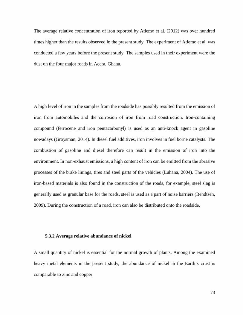
73

The average relative concentration of iron reported by Atiemo et al. (2012) was over hundred

times higher than the results observed in the present study. The experiment of Atiemo et al. was

conducted a few years before the present study. The samples used in their experiment were the

dust on the four major roads in Accra, Ghana.

A high level of iron in the samples from the roadside has possibly resulted from the emission of

iron from automobiles and the corrosion of iron from road construction. Iron-containing

compound (ferrocene and iron pentacarbonyl) is used as an anti-knock agent in gasoline

nowadays (Groysman, 2014). In diesel fuel additives, iron involves in fuel borne catalysts. The

combustion of gasoline and diesel therefore can result in the emission of iron into the

environment. In non-exhaust emissions, a high content of iron can be emitted from the abrasive

processes of the brake linings, tires and steel parts of the vehicles (Luhana, 2004). The use of

iron-based materials is also found in the construction of the roads, for example, steel slag is

generally used as granular base for the roads, steel is used as a part of noise barriers (Bendtsen,

2009). During the construction of a road, iron can also be distributed onto the roadside.

5.3.2 Average relative abundance of nickel

A small quantity of nickel is essential for the normal growth of plants. Among the examined

heavy metal elements in the present study, the abundance of nickel in the Earth’s crust is

comparable to zinc and copper.

74

G7

: W

art

ko

wic

e

G6

: R

aw

a M

az.

I

G1

6:

Ra

wa

Ma

z. I

I

G1

8:

Lo

wic

z

G3

4:

city

of

Lo

dz

G2

7:

Na

kh

on

Si.

I

G2

8:

Na

kh

on

Si.

II

New

Zea

lan

d -

Wa

rd e

t a

l.

19

77

Tu

rkey

-

Sez

gin

et

al.

20

03

0.01

0.1

1

10

PL TH OTHER

Av

erag

e re

lati

ve

ab

un

da

nce

of

nic

kel

Research sites

Figure 5.3 The average relative abundance of nickel in roadside plants of the different studied

sites. Detailed description as in Fig 5.2

The enhanced levels of nickel, above the unpolluted samples, were observed only at the studied

sites in Poland. At the studied sites in Thailand (G27 and G28), although the average relative

abundances of nickel were close to those in the plants at unpolluted sites, a high average relative

abundance of the nickel compared to the new road was observed.

The differences of average relative abundances of nickel between the new roads and the old

roads, in Fig 5.3, are clearly noticed. The enhanced average abundances of nickel (above the

unpolluted samples) in the plant samples are distinguished for the studied sites in Poland (G7,

G6, G16, G18 and G34).

75

Average relative abundances of nickel observed at the roadside of the Auckland motorway

(Ward et al., 1977) and the Istanbul E-5 highway (Sezgin et al., 2003) were comparable to those

of the new roads in the present study.

The results of Ward et al. were obtained by the study of pasture species (perennial ryegrass,

white clover, cocksfoot, Yorkshire fog, daisy, pastalum grass and flatweeds) growing on the

median strip along the Auckland motorway roadside in New Zealand. This motorway had the

traffic density in the similar range of the present study (20,000 – 70,000). In the study of Ward

et al., the enhanced levels of cadmium, chromium, nickel, zinc and lead were found and seemed

to be correlated well with the traffic rates.

In the year of 2002, Sezgin et al. conducted a similar experiment at the roadside of the Istanbul

E-5 highway in Turkey. The samples of street dust from 14 sites were examined in their

experiment. Nickel concentrations measured at the most of their studied sites were found within

natural limits.

A measurable amount of nickel is also found in gasoline, both regular and premium grade,

(Jungers et al., 1975). It is possible that the process of oil combustion of automobiles contributes

in emitting nickel pollution onto the roadside (Swietlicki and Krejci, 1996).

76

5.3.3 Average relative abundance of zinc

Zinc is a toxic metal element. However, for plants, a small quantity of zinc is an important

structural constituent of enzymes necessary for healthy growth and also carbohydrate and

protein metabolism.

G7

: W

art

ko

wic

e

G6

: R

aw

a M

az.

I

G1

6:

Ra

wa

Ma

z.

II

G1

8:

Lo

wic

z

G3

4:

city

of

Lo

dz

G2

7:

Na

kh

on

Si.

I

G2

8:

Na

kh

on

Si.

II

En

gla

nd

-

Ha

rri

son

et

al.

1981

Ho

ng

Ko

ng -

Wo

ng a

nd

Ma

k

1997

Tu

rkey

-

Sez

gin

et

al.

2003

0.1

1

10

100

Av

erag

e re

lati

ve

ab

un

da

nce

of

zin

c

Research sites

PL TH OTHER

Figure 5.4 The average relative abundance of zinc in roadside plants of the different studied


An apparent low relative abundance of zinc at the studied site G28 can be seen (Fig 5.4). Prime

consideration should be given here to the soil condition. Next to the sampling areas of the site

77

G28 which was waterlogged. This condition probably gives rise to the lack of zinc on the soil

surface where the plants grow (Alloway, 2008).

The average relative abundances of zinc of all studied sites in the present study corresponded to

the behaviour of iron. The results obtained from the new roads were significant higher than those

from the old ones, except the site G28.

In the work of Harrison et al. (1981), they examined street dust and roadside soil from some

major roads in England. They found out that the samples collected from the highest traffic site

contained a considerable amount of zinc. The same finding was also made by Sezgin et al.

(2003) from the study of road dust on the Istanbul E-5 highway in Turkey. When compared to

the present study, the relative levels of zinc from the studies of Harrison et al. and Sezgin et al.

are consistent with the results from the old roads (except the site G28).

Wong and Mak (1997) conducted the experiment in 1993. In their experiment, dust and soil

samples obtained at children playgrounds located next to the roads in Hong Kong were used in

the examination of heavy metal elements (cadmium, copper, zinc and lead). They found a high

correlation between contents of the heavy metal elements and traffic densities and between the

contents of zinc and lead. The relative levels of zinc from the present study of Wong and Mak

were consistent with the new road from the present study.

The emission of zinc from the vehicular traffic is usually assigned to the corrosion of tires.

Because in the general industrial processes of vulcanization, a high content of zinc oxide is

added.

78

5.3.4 Average relative abundance of lead

Lead is known as a toxic metal element which can constitute health hazard to humans and

animals. In living organism, lead can be found in a trace level, however its function is still

questionable.

The content of lead in plants generally reflects its availability in the ecological system where

the plants grow (Lepp, 1981). Lead is available to plants from soil and aerosol sources. The

plants growing on the roadside are usually exposed to more lead than other locations (Zimdahl

and Hassett, 1977).

G7

: W

art

kow

ice

G6

: R

aw

a M

az.

I

G1

6:

Ra

wa

Ma

z. I

I

G1

8:

Lo

wic

z

G3

4:

city

of

Lo

dz

G2

7:

Na

kh

on

Si.

I

G2

8:

Na

kh

on

Si.

II

En

gla

nd

-

Ha

rris

on

et

al.

19

81

Ho

ng

Ko

ng

-

Wo

ng

an

d M

ak

19

97

Tu

rkey

-

Sez

gin

et

al.

20

03

Gh

an

a -

Ati

emo

et

al.

20

12

0.01

0.1

1

10

Av

era

ge

rela

tiv

e a

bu

nd

an

ce o

f le

ad

Research sites

PL TH OTHER

Figure 5.5 The average relative abundance of lead in roadside plants of the different studied


79

The results of lead from all studied sites in the present study were found in the similar pattern

to nickel. The average relative abundances of lead in the samples collected from the old roads

were significantly higher than those from the new ones and also higher than those from the

unpolluted areas, see Fig 5.5.

Similar studies were conducted in England, Hong Kong, Turkey and Ghana by four different

research groups. These groups indicated that the samples from their studied sites were highly

contaminated with lead. Their results, when compared to the present study, were in accordance

with the results from the old roads.

Lead-containing anti-knock agent (tetraetthyl lead and tetramethyl lead) was used intensively

before being phased-out in some countries in the late 19th century7. At the present time, the

content of lead in gasoline can be detected on a trace level, lower than iron, nickel, copper and

zinc. After the combustion of gasoline in a car engine, lead is emitted into atmosphere and then

deposited in soil and throughout the ecological system. The plants which are growing at the

areas exposed to lead for a long period of time, like at the site G18, G34, G27 and G28, can

accummulate more lead than the plants at the younger sites like G7, G6, and G16.

Another possible source of lead, together with nickel, that should be also noted here is fertilizers

application on farmlands. A commercial phosphate fertilizer generally contains varied types of

heavy metal elements (Mortvedt, 1995) such as cadmium, arsenic, chromium, lead, mercury,

7 Leaded gasoline banned in, for example, Poland in 2005, Thailand in 1996, England in 1998, Hong Kong in

1999, Turkey in 2006, Ghana in 2002.

80

nickel and vanadium. If this fertilizer is applied and the procedure is repeated in an area near to

the road, the soil in that area can become highly contaminated with lead and nickel. The studied

sites which could be possibly become affected by lead- and nickel-containing fertilizers were

G6 and G18, because on one side of the roads of these two sites were close to agricultural areas.

5.3.5 Average relative abundances of bromine, rubidium and strontium

It was found that the average relative abundances of bromine, rubidium and strontium vary

among all studied sites. The influence of the age of the road on the abundances was not observed.

Bromine is one of the metal elements considered to be very toxic. It was found on a trace level

in humans, animals and plants, however its essential role is still not known.

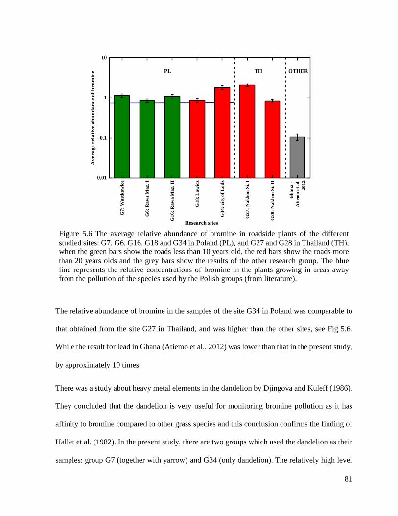
81

G7

: W

artk

ow

ice

G6

: R

aw

a M

az. I

G1

6:

Ra

wa

Ma

z. II

G1

8:

Lo

wic

z

G3

4:

cit

y o

f L

od

z

G2

7:

Na

kh

on

Si.

I

G2

8:

Na

kh

on

Si.

II

Gh

an

a -

Ati

em

o e

t a

l.

20

12

0.01

0.1

1

10

Av

erag

e r

ela

tive a

bu

nd

an

ce o

f b

rom

ine

Research sites

PL TH OTHER

Figure 5.6 The average relative abundance of bromine in roadside plants of the different

studied sites: G7, G6, G16, G18 and G34 in Poland (PL), and G27 and G28 in Thailand (TH),

when the green bars show the roads less than 10 years old, the red bars show the roads more

than 20 years olds and the grey bars show the results of the other research group. The blue

line represents the relative concentrations of bromine in the plants growing in areas away

from the pollution of the species used by the Polish groups (from literature).

The relative abundance of bromine in the samples of the site G34 in Poland was comparable to

that obtained from the site G27 in Thailand, and was higher than the other sites, see Fig 5.6.

While the result for lead in Ghana (Atiemo et al., 2012) was lower than that in the present study,

by approximately 10 times.

There was a study about heavy metal elements in the dandelion by Djingova and Kuleff (1986).

They concluded that the dandelion is very useful for monitoring bromine pollution as it has

affinity to bromine compared to other grass species and this conclusion confirms the finding of

Hallet et al. (1982). In the present study, there are two groups which used the dandelion as their

samples: group G7 (together with yarrow) and G34 (only dandelion). The relatively high level

82

of bromine observed at the site G34 compared to the other sites in Poland, is probably not cause

only by the fact that this site is located in the city center which has high traffic rate, but also due

to the fact that the dandelion itself can accumulate a high content of bromine. For the other

species of the studied plants, ability of bromine absorption was not documented.

At the time when leaded gasoline was used, bromine and lead were bound in the fuel additive.

The correlation between bromine and lead was observed by many research groups (e.g., Oblad

and Selin, 1985; Djingova et al., 1986; Capannesi et al., 1993; Lammel et al., 2002; Bennet et

al., 2005).

The results from the present research were not clear in regards to the high average relative

abundances of lead entailed the high average relative abundances of bromine. For example, if

the lead and bromine were deposited together in a sample, the results of lead (Fig 5.5) from the

site G18 and G28 should be as high as the results of bromine (Fig 5.6). However, in fact, the

relative abundances of lead of those two sites seemed to be lower than those of bromine. This is

probably caused by the removal of some bromine in gaseous form (Farmer and Cross, 1978;

Alov et al., 2001). In automobile engines, after the combustion of leaded gasoline, mixed

halogenides of lead can be formed (PbBrCl). This compound can be photochemically

decomposed into lead and halogens (bromine and chlorine). Lead perhaps recombinates as a

lead compound of acidic ammonium sulphate (PbSO4(NH4)2SO4), while the latter perhaps

recombinates as halogen molecules or halide compounds. The halide compound of bromine

called hydrogen bromide (HBr) is a gas which is very soluble in water, while lead compound is

83

less soluble. The regular washing of hydrogen bromide can occur by, for example, precipitation

and surface water runoff. Furthermore, the hydrogen bromide in the air can be transported for a

longer distances as it has a molecular mass smaller than that of the lead compound.

In relation to pollution on the roadside, rubidium as well as strontium were not studied

extensively as the other heavy metal elements (e.g., iron, nickel, zinc and lead). This was

because automobiles are not considered to be their main source and these two elements generally

do not cause a health risk.

G7:

Wartk

ow

ice

G6:

Raw

a M

az. I

G16:

Raw

a M

az. II

G18:

Low

icz

G34:

cit

y o

f L

od

z

G27:

Nak

hon

Si.

I

G28:

Nak

hon

Si.

II

Gh

an

a -

Ati

em

o e

t al.

2012

0.01

0.1

1

10

100

Average r

ela

tive a

bu

nd

an

ce o

f ru

bid

ium

Research sites

PL TH OTHER

Figure 5.7 The average relative abundance of rubidium in roadside plants of the different

studied sites: G7, G6, G16, G18 and G34 in Poland (PL), and G27 and G28 in Thailand (TH),

when the green bars show the roads of less than 10 years old, the red bars show the roads of

more than 20 years olds and the grey bars show the results of the other research group.

84

In Fig 5.7, evidence can be pointed out here that the average relative abundances of rubidium

from the studied sites in Thailand was higher than in Poland and Ghana.

The average relative abundances of strontium is shown in Fig 5.8.

G

7:

Wa

rtk

ow

ice

G6

: R

aw

a M

az.

I

G1

6:

Ra

wa

Ma

z. I

G1

8:

Lo

wic

z

G3

4:

city

of

Lo

dz

G2

7:

Na

kh

on

Si.

I

G2

8:

Na

kh

on

Si.

II

Gh

an

a -

Ati

emo

et

al.

2012

0.1

1

10

100

Av

era

ge

rela

tiv

e a

bu

nd

an

ce o

f st

ron

tiu

m

Research sites

PL TH OTHER

Figure 5.8 The average relative abundance of strontium in roadside plants of different studied

sites. Detailed description as shown in Fig 5.7

Except for the “urban” site G34, in the city of Łódź (Fig 5.8), the average relative abundances

of strontium do not fluctuate as much as the rest of studied sites, including in Ghana.

85

If the abundance of strontium in plants is mainly derived from soil, it is possible that a high

deposition of heavy metal pollution in the city diminishes the existence of native soils like in

the case of the site G34 for example.

86

5.4 Distribution of the heavy metals with respect to the distance of the road

axis

Below an analysis of the elemental distribution made by the group G7 was presented, as an

example, based on the results obtained by this group. The rest of students’ results is shown in

Appendix B.

5.4.1 The studied site G7 (Wartkowice, Poland)

The heavy metal elements in the roadside plants at the studied site G7 were examined

by the students of Gimnazjum Zespołu Szkół in Wartkowice. The studied site is located next

to the four-lane A2 motorway, part of the expressway E30, section Konin Zachód – Stryków,

in the village of Powodów. It is about 6 km away from the students’ school and it runs from the

west of the German border through central Poland (Poznań and Łódź) to the east (Warsaw). The

motorway was opened in July 2006. The plant samples, dandelion and yarrow, were collected

in the autumn 2013, from the roadside where the provincial road (of the province of Łódź) 469

crosses the motorway, see Fig 5.9. This provincial road was constructed in the 1980’s. The

traffic rate on this road was about 50,000 units per day.

87

(a)

(b)

Figure 5.9 The studied site G7 (a) shows a satellite view of the GPS coordinate (51.97301,

19.08861), and (b) shows the site plan with the research areas (green blocks) where the

samples were collected (no sample is available on the research area 0AR, 25AR, 0AL, 0BL

and 25CL).

On the left, the studied site was bounded by the noise barriers of the height of about 3.5 m (next

to the motorway edge), the provincial road 469 (next to grid CL), and a local road (next to grid

50L). On the right, the studied site was bounded by the provincial road 469 (next to grid CR and

grid 50R), see Fig 5.9 (b). The students chose this site because they expected to see the effect

of the noise barriers on the left side of the road. This is an example of the extra activity

88

undertaken by the children. However, this site was not the best choice for the research. Results

from the studied site G7 are shown in Fig 5.10.

50L 25L 0L road axis 0R 25R 50R

0.1

1

10R

ela

tiv

e a

bu

nd

an

ce

Distance from road edge (m)

site G7: Wartkowice

Figure 5.10 The lateral distribution of heavy metal relative abundances with respect to copper

(Cu = 1) in the roadside plants from the studied site G7 ( - Fe, - Ni, - Zn, - Pb,

- Br, - Rb and - Sr)

On the right roadside, only iron clearly showed a decrease with the distance to the road. The

levels of nickel, zinc, lead, bromine, rubidium and strontium in the samples at the road edge

were systematically higher than at the distance of 25 m from the road edge. However their levels

at the distance of 50 m returned to or were close to their levels as found in the samples at the

road edge. It can be explained by the existence of the local road close to the 50R points.

On the left roadside, the levels of a majority of the elements behind the noise barriers, were

slightly lower.

89

5.4.2 The final analysis of all collected data

The individual results from all groups analyzed together showed that the relative abundances of

the heavy metal elements in the samples at most of the studied sites were decreasing in a

perpendicular direction to the road edge.

The data which were marked also by the children as “biased” (see Appendix B) and excluded

from our final analysis. The “biased” results covered “construction area” (G6), “urban area”

(G34) and “small statistic” (G28).

For the rest four groups, the element showing clearly the decrease pattern was fit with one

exponential function as in the work of Schuck and Locke (1970), for each site

N(r) = N0e−r

r0⁄ (5.1)

the parameter r0 can be interpreted as an average characteristic decrease length of general

“heavy metal pollution” generated by the traffic at the particular site. Results are shown in Fig

5.11 and in Table 5.3.

90

0 25 500.0

0.5

1.0

Rel

ativ

e abundan

ce

Distance (m)

G7: Wartkowice

N(r) = 0.9 e (-r/91)

(a)

0 25 500.0

0.5

1.0

1.5

2.0

Ele

men

tal

abu

nd

ance

Distance (m)

G16: Rawa Maz. II

N(r) = 1.7 e (-r/40)

(b)

0 25 500.0

0.5

1.0

1.5

Ele

men

tal

abundan

ce

Distance (m)

G18: Lowicz

N(r) = 1.1 e (-r/56)

(c)

0 25 500.0

0.5

1.0

1.5

2.0

2.5

Ele

men

tal

abu

nd

ance

Distance (m)

G27: Nakhon Si. I

N(r) = 1.5 e (-0.014r)

(d)

Figure 5.11 The exponential models of the decreasing relative abundances of heavy metal

elements in the samples at the studied site (a) G7 (Wartkowice), (b) G16 (Rawa Mazowiecka),

(c) G18 (Łowicz) and (d) G27 (Nakhon Si Thammarat I) ( - Fe, - Ni, - Zn, - Pb,

- Br, and - Rb)

Some comments on the existing barriers and the traffic rates for analysis of the possible effect

of the decrease of heavy metal elements in the plant samples were also added, see Table 5.3.

91

Table 5.3 Height of the barriers, traffic rates and decreasing parameter r0 at the studied site G7,

G16, G18 and G27

Studied sites Height of barriers

(m)

Traffic rates

(units per day)

Decreasing parameter r0

(m)

G7: Wartkowice 3.5 50,000 91

G16: Rawa Maz. II no barrier 48,000 40

G18: Lowicz 3 – 5 26,000 56

G27: Nakhon Si. I no barrier 50,000 71

It can be indicated that, if the effect of barriers exist, it has a very local characteristic and the

height of the barriers is only one of many parameters responsible for the pollution distribution.

Concerning the traffic rates, unfortunately there were 3 of 4 sites with very similar traffic rates.

So no conclusion can be provided here.

0 25 500.0

0.3

0.6

0.9

1.2

1.5

Rel

ati

ve

ab

un

dan

ce

Distance (m)

Figure 5.12 Combined data from the studied site G7, G16, G18 and G27 where decreasing

relative abundance pattern of the heavy metal elements can be seen ( - Fe, - Ni, - Zn,

- Pb, - Br, - Rb and - Sr).

92

The combined data from all four studied sites are presented in Fig 5.12 for the separate elements.

The systematic decreases of relative abundances of iron, nickel, zinc, lead and bromine is seen.

No clear effect is observed for the relative abundances of rubidium and strontium.

5.4.3 Comparison of the average characteristic decrease length of iron with other

results

The fit of iron from the results provided by the present study compared to the results from the

experiment at the Moscow highways in Russia performed by Alov et al. (2001) is shown in Fig

5.13.

0 25 500.0

0.2

0.4

0.6

0.8

1.0

1.2

1.4

e (-r/83)

e (-r/34)

the present study

Alov et al. 2001

Rel

ati

ve

ab

un

dan

ce o

f ir

on


Figure 5.13 Comparison of the average characteristic decrease length of iron of the present study

(black solid marks) to the similar study at the Moscow highways by Alov et al. (red square

marks).

93

The average characteristic decrease length of iron of the present study is 2.4 times shorter than

one of the Moscow highways.

The study of iron pollution at the Moscow roadside was conducted over 10 years ago. The

samples used in the study were the soil from the ground surface at the distance 10 – 200 m. The

traffic rate of the highways was not given in the research paper. It was found that the

concentrations of iron in the samples decreased with the distance within 100 m from the road

edge. After the distance of 150 m, the similar decrease was not be observed.

5.4.4 Comparison of the average characteristic decrease length of nickel with other

results

The results of the present study (Fig 5.14) are consistent with the experiment of Zhao et al.

(2010) in China. Their experiment showed the characteristic decrease length above 100 m.

While the experiment of Largerwerff and Specth (1970), in USA, reported a much shorter

characteristic decrease length. This experiment was conducted among two roads with the traffic

rates of 20,000 and 48,000 units per day, respectively. The results in Fig 5.14 were obtained

from the examination of grass growing on the roadside at the distance within 32 m from the road

edge.

94

0 25 50 75 100 125 150 175 200 2250.0

0.2

0.4

0.6

0.8

1.0

1.2

1.4

1.6

e (-r/42)

e (-r/125)

e (-r/186)

the present study

Lagerwerff and Specth 1970

Zhao et al. 2010

Rel

ati

ve

ab

un

da

nce

of

nic

kel


Figure 5.14 Comparison of the average characteristic decrease length of nickel of the present

study (black solid marks) to the similar studies at USA by Lagerwerff and Specth (red marks)

and China by Zhao et al. (blue marks)

The experimental results of Zhao et al. were obtained by using the samples of two different

species of grass. These samples were collected at the downslope areas located next to the roads

of the traffic rates of 40,000 and 60,000 units per day. This traffic rate was equivalent to the

studied sites of the present study, but it was higher than the one in USA.

5.4.5 Comparison of the average characteristic decrease length of zinc with other

results

The average characteristic decrease length of zinc from the present study was situated between

the results from the experiment in USA (Largerwerff and Specth 1970) and France (Viard et al.

2004), see Fig 5.15.

95

0 25 50 750.0

0.2

0.4

0.6

0.8

1.0

1.2

1.4

e (-r/26)

e (-r/67)

e (-r/167)

the present study


Viard et al. 2004

Rela

tiv

e a

bu

nd

an

ce

of

zin

c


Figure 5.15 Comparison of the average characteristic decrease length of zinc of the present study

(black solid marks) to the similar studies at USA by Lagerwerff and Specth (red marks) and

France by Viard et al. (blue marks)

The experiment in France was conducted in the vicinity of the A31 highway between the city of

Nancy and the border of Luxembourg. The samples of atmospheric deposits were collected

within the distances up to 320 m from the highway.

5.4.6 Comparison of the average characteristic decrease length of lead with other

results

Lead is considered as having the most toxic elements emitted from vehicles. The distribution of

lead in the vicinity of the roads was studied by many research groups.

96

The average characteristic decrease length of lead from the present study was perfectly

consistent with the experimental result from Syria (Othman et al., 1997). Both results, however,

were greater than the results from the other sites (Lagerwerff and Specth, 1970; Viard et al.,

2004; Zhao et al., 2010).

0 20 40 60 80 100

0.0

0.3

0.6

0.9

1.2

1.5

1.8

2.1

2.4

e (-r/111)

e (-r/59)

e (-r/43)e

(-r/26)

e (-r/100)

the present study


Othman et al. 1997

Viard et al. 2004

Zhao et al. 2010

Rel

ati

ve

ab

un

da

nce

of

lea

d


Figure 5.16 Comparison of the average characteristic decrease length of lead of combined data

of the four studied sites from the present study (black solid marks) to the similar studies in USA

by Lagerwerff and Specth (red marks), Syria by Othman et al. (yellow marks), France by Viard

et al. 2004 and China by Zhao et al. 2010 (green marks)

The experimental results at Syria (Fig 5.16) were obtained from the examination of lead in

vegetable species growing in agricultural land next to the roads in the City of Damascus. The

traffic rates of the two roads were about 40,000 units per day.

97

5.4.7 Average characteristic decrease length of bromine

The average characteristic decrease length of bromine is shown in Fig 5.17. No experimental

results concerning the distribution of this element aside the road has been published yet.

0 25 500.0

0.3

0.6

0.9

1.2

e (-r/56)

Rel

ati

ve

ab

un

da

nce

of

bro

min

e


Figure 5.17 The average characteristic decrease length of bromine from the present study

The average characteristic decrease length of bromine pollution from the analysis of the present

study was 56 m which was close to the one obtained for the zinc.

98

5.4.8 Summary of the average characteristic decrease length of the heavy metal

pollution

The results shown in Fig 5.13 – 5.17 are summarized in Table 5.4.

Table 5.4 Comparison of the average characteristic decrease length (parameter r0) of the present

study to the experimental results of the other studies

Research groups Sample types Traffic rates

Decreasing parameter R0

(m)

Fe Ni Zn Pb Br

The present study Herb 26,000 – 50,000 34 125 67 100 56

Lagerwerff and

Specht (1970) Grass 20,000 – 48,000

- 42 167 26 -

Othman et al. (1997) Vegetable 35,000 – 39,000 - - - 111 -

Alov et al. (2001) Soil - 83 - - - -

Viard et al. (2004) Atmospheric

deposit 40,000 – 60,000

- - 26 59 -

Zhao et al. (2010) Herb 40,000 – 60,000 - 186 - 43 -

The average characteristic decrease length for the heavy metal elements was in a range of 50 –

150 m, with the ordered pattern: nicke > lead > zinc > bromine > iron. No dependence on a

particular analyzed plant species was observed. The measurement of the present study was

consistent, in general, with the existing literature values.

The more accurate values of the average characteristic decrease length of particular elements

will be calculated when more experimental data which is to be obtained in the future from

worldwide school students who participate in the “nuclear e-cology” project. These values will

be regarded as a “finger print” of the human-origin heavy metal elements, which originated from

the automobiles on the roads.

99

6 CONCLUSION REMARKS

According to the study of human-origin heavy metal pollution on the roadside by using X-ray

spectroscopy,

(1) I discovered that the average relative abundances of nickel and lead in the studied

plants collected from the new roads were a few times lower than those from the old ones.

Other elements like iron and zinc showed the similar relation to the age of the road as to

the time for each of the pollution to have been deposited;

(2) I found that the relative abundances of iron, nickel, zinc and lead decreased as a

function of distance from the road with the average characteristic decrease length of 50 –

150 m;

(3) I observed the distribution of bromine aside the road for the first time. The relative

abundance of the bromine decreased with the distance from the road with the average

characteristic decrease length of 60 m;

(4) I found that the average abundances of rubidium and strontium did not decrease with

the distance from the road. This suggested that the traffic is probably not a source of these

two metal elements observed in the samples of the present study;

(5) I developed a method of engaging school students in the present research. This allowed

us to obtain experimental data from different reseach sites across the world.

The further study is to collect more experimental data, extending to other countries.

100

7 POSSIBILITY TO CONTINUE THE RESEARCH

The groups from the 2013/2014 project, which have not finished the study, could continue their

study in 2015. For the next edition, the 2014/2015 project was opened for new registration

starting from January to April 2015. In the new edition, there were two experimental lessons

offered the participants to choose from. The first one was still on the examination of heavy metal

elements in roadside plants. The second one had the same idea to the first lesson but instead of

studying impacts of pollution along the road, the participants had to conduct that study on water

resources e.g., river, lake and reservoir by examining some heavy metal elements in lesser

duckweed (Lemna minor L.) – aquatic plant.

In January 2015, we got 6 new groups (4 groups from Poland and 2 groups from Thailand). At

this moment, February 2015, they were collecting the samples.

About the myself, although, I had to return back to my home country which is Thailand at the

end of my study. I still had the intention to continue working on the project. I would like to

establish another center of the Educational Nuclear e-Laboratory in Thailand. One idea of mine

was: in Europe we already had the lab center established in Poland, but if there was also one in

Asia, a lab center in Thailand for example. The laboratory in Thailand could provide the

participants within county and from neighboring countries with convenience on delivery of the

samples.

For X-ray spectrometer, at the beginning, I already had a plan to use the spectrometer and lab

facilities at the Synchrotron Light Research Institute in Nakhon Ratchasima, which is a province

in the the North East of Thailand. At the same time, I would like to apply for a research grant in

101

order to establish my own X-ray laboratory for long term use. I also expected to have scientists

(collaborative team) who can be the specialists in biology, environmental science, and physics

education in Thailand and Asian context.

Especially, in 2015, the association of Southeast Asia Nations (ASEAN) had strategic schedule

for the ASEAN Economic Community. In a strategic approach for the freer flow of capital,

every country in ASEAN Economic Community had to take action on an arrangement for the

cross recognition of qualifications, education and experienced market professionals. Thailand

aims at becoming the Education Hub of the ASEAN Economic Community. Various

government policies will facilitate the active research collaboration in education, science and

technology amongst many universities and institutes of science, in order to educate and prepare

people to be able to work in ASEAN.

Due to the character of the “nuclear e-cology” project (including the project of remote

laboratories in different fields of physics), it enables us to work with students, and researchers

in ASEAN and worldwide countries. The collaborative research activities can enhance growth

and productivity in science and education. Moreover; this project can result in providing the

young people not only with scientific knowledge, but also with public awareness of the

environment.

Having taken all the facts and data from the extensive research in putting this ongoing project

together. It is recommended that this project is sufficiently valuable to justify the investment of

time, interest, and finance, so it can be continued in Thailand.

102

8 SUMMARY

The relative abundances of iron, nickel, zinc, lead, bromine, rubidium and strontium in roadside

plants along different studied sites in Poland and Thailand were examined using the X-ray

fluorescence spectrometry method. The results from the partial reports of school-student teams

constituted input data for the final analysis as a part of which the school students performed the

experiment following the prepared instruction, under supervision of the scientists, aided by the

Internet communication.

It was found that the heavy metal pollution observed in the analyzed samples, especially for

nickel and lead did depend on the age of the road. The plant samples collected from the sites of

the road of the age less than 10 years showed the average relative abundances a few times

smaller than those observed in the samples collected at the sites close to the road of the age

higher than 20 years.

It was found that the relative abundances of iron, nickel, zinc, lead and bromine decreased with

the increase of the distance from the road. This confirms the effect of the transport as a source

of pollution.

The average characteristic decrease length of the relative abundances of iron, nickel, zinc and

lead was measured in the present study. It was in the range of 50 – 150 m. Furthermore, for the

first time, the decreasing amount of relative abundance of the bromine was measured. The

average characteristic decrease length of bromine was at the level of 60 m.

103

It was established that the relative abundances of rubidium and strontium did not exhibit a

regular gradient as a function of distance from the road. These two heavy metal elements were

probably not derived mainly from the traffic.

The research of examination of some heavy metal pollution in roadside plants is being continued

as a part of the research project entitled “nuclear e-cology”, which is an ongoing observation of

heavy metal pollution from roadside around the world by involving the school students in the

scientific research.

104

APPENDIX A LEARNING MATERIALS AND ACTIVITIES

FOR THE PARTICIPANTS OF THE “NUCLEAR E-COLOGY”

PROJECT

A.1 Video instruction

The first video clip was produced to introduce the Gaussian-fit program, and learn how to fit

the background and peaks of the spectrum data by using the program.

Figure A.1 A screenshot of the video instruction “how to fit background and peaks” which

shows a demonstration of fitting the background of an X-ray spectrum.

The content of the video clip “how to fit background and peaks” consisted of the instruction

concerning:

(1) the Gaussian-fit program, such as how to install the program, how to download a data

file, how to display graph and how to manipulate the line profile;

105

(2) the spectrum data, such as the meaning of background and peaks, fluorescence peaks

and X-ray emission lines;

(3) the best fit, such as how to fit the line profile to the background and fluorescence

peaks and what parameters define the background and peaks;

(4) the exercise, such as what individual participant was assigned to do in order to

complete the exercise, how to complete the answers and how to submit the answers and

process them after submission.

The second video clip was devoted the lab standard form of the group report. Before analyzing

data and writing a group report, the participants may learn from this video footage.

Figure A.2 A screenshot of the video instruction “how to write a group report” which shows

the standard report form in an Excel spreadsheet.

The content of the “how to write group report” video clip covered the following instruction:

106

(1) the standard group report form, such as where to download the form, what application

is to be used when working with the form, what the three parts of the report (results, graphs

and discussion, and conclusion) are, what information is needed to fill in the form, how to

match the codes of the studied sites to the spectrum data and tables, where to find the

spectrum data files in the group page, how to fill fitting the results into the tables of data,

what parameters are to be filled in the tables of data and what is to be automatically

calculated and graphed in the data sheets;

(2) the normalization, such as interpretation of normalization and use of normalized data

in graphing and data analysis;

(3) the process after a submission of the group report.

The video clip devoted to “how to write group report” was embedded at the page “analyze data

and write report” together with the third video showing an example of research papers as a guide

on explaining how to write a group report.

Figure A.3 A screenshot of the video instruction “research paper” which shows how to present

research results using graphs.

107

An example of a research paper was presented to the participants in order to show them what

the real scientific research paper looks like. The research paper example was obtained from the

study of lead levels in roadside soils and vegetation of Damascus city written by Othman et al.

(1997) published in an international journal of Science of the Total Environment. This research

was in the same field of our interest. The presentation of the information in the paper guided the

students on how to write the group report.

We also provided the participants with more examples of research papers as regards the lesson.

They were available on the webpage.

The fourth video clip was devoted to the sample preparation and the measurement of the samples

using the X-ray spectrometer. This video clip was posted on the group page.

Figure A.4 A screenshot of the video instruction concerning “sample preparation and

measurement” which shows the sample treatment for measurement with the TXRF technique.

This video clip of “sample preparation and measurement” was produced to show the process

after the samples were delivered to the laboratory: measuring the samples, wet digestion and

108

dilution, the process of drying the samples on carriers, and measurement with the spectrometer.

In this video, we also presented some examples of the accumulation of spectra during the

measurements.

109

A.2 The “nuclear e-cology” webpage

The site map in Fig 4.5 starts from a home page where the web users can find information about

the “nuclear e-cology” project and learn how to take part in the experimental lesson. At any

page of the website, the web users can link to the other pages using 13 menu bars:

(1) menu bar “updates” links to:

o “news” page containing the announcements of events, messages to participants

from the laboratory and status of the groups’ activities;

o “activity calendar” page containing a register of events of the “nuclear e-cology”

laboratory;

o “map of studied site” page containing the map of the studied sites (Google Map);

(a)

Figure A.5 Screenshots from the “nuclear e-cology” website of the “news” page show an

access to (a) the experimental results database (from group reports) and (b) the individual

group activity pages.

110

(b)

Figure A.5 (Continue)

(2) menu bar “students” links to:

o “student guide” page containing the list of what the participants have to do

starting from registration to completion of the experimental lesson;

o “individual registration” page containing the online form of individual

registration;

o “group registration” page containing the online form of group registration;

o “list of participants” page containing the list of members of a particular group.

This page links to the “group” pages (each group has its own page). A “group” page

contains the information about the experiment conducted by the group, in details of

their studied site, samples, X-ray spectrum files and group report;

(3) menu bar “teachers” links to:

o “list of teachers” page containing the list of teachers of a particular group;

o “teacher registration” page containing the online form of the teacher registration;

o “survey” page containing the online survey for teachers;

111

(4) menu bar “test” links to the initial test for the school students;

(5) menu bar “X-ray” links to:

o “discovery of X-rays” page containing the information about the discovery

of X-rays by Wilhelm Konrad Roentgen and the properties of X-rays;

o “generation of X-rays” page containing the information about X-ray generation

in an X-ray tube, X-ray radiation in an atom and X-ray emission lines;

o “X-ray spectrometer” page containing the information about the general

principle of an X-ray spectrometer;

(6) menu bar “experimental lessons” links to:

o “lesson 1 roadside plants” pages containing the laboratory direction of

the experimental lesson on the examination of heavy metal elements in roadside

plants, including guides of the given plant species and safety in fieldwork;

o “lesson 2 aquatic plant” pages containing the laboratory direction of

the experimental lesson on the examination of heavy metal elements in the aquatic

plant;

(7) menu bar “software for spectrum analysis” links to “Gaussian-fit” page containing

the information about the installation of the Gaussian-fit program, instructions with

video clips, and exercise;

(8) menu bar “lab facilities” links to “lab instrument” page containing the information

of the X-ray Spectrometry Laboratory in Kielce and the details of the TXRF

spectrometer used in the present research;

112

(9) menu bar “lab team” links to:

o “general physics team” page containing a brief biography and contact

information of the scientists of the general physics team;

o “biology and environmental science team” page containing a brief biography and

contact information of the scientists of the biology and environmental science team;

o “X-ray spectrometry laboratory team” page containing a brief biography and

contact information of the scientists of the X-ray spectrometry laboratory team;

(10) menu bar “contact us” links to the contact information (address, e-mail and video

call) of the “nuclear e-cology” laboratory;

(11) menu bar “publications” links to:

o “conferences” page containing the list of the studied topics presented at the

conferences;

o “papers” page containing the list of research papers published in journals;

(12) menu bar “FAQ” links to the answers of frequently ask questions;

(13) menu bar “other links” links to the Interactive Aerodynamic Wind Tunnel website

(another project in physics education of the Chair of Modelling Teaching Processes,

Faculty of Physics and Applied Informatics, University of Łódź and other websites

related to physics events and activities organized by University of Łódź for teachers and

school students.

113

(a)

(b)

(c)

Figure A.6 Screenshots from the “nuclear e-cology” website of (a) the “X-ray” pages, (b)

plant species descriptions and (c) the “software for spectrum analysis” pages

114

A.3 Facebook page of the project

Apart from the project website, the participants can also follow updated activities,

announcements, video clips, and events, open a topic for discussion, and question to scientists

and the other participants via Facebook page of the “nuclear e-cology” community. We found

that using the Facebook page enables us to promote the project to other Facebook users (e.g.,

participants’ and our friends who use Facebook) and enables the participants to reach the news

from the laboratory fast and easily.

115

Figure A.7 A screenshot of the Facebook page of the “nuclear e-cology” project which shows

announcements and photos from updated activities

However, the Facebook page was used only for feeding news and announcements. If one wishes

to know what is going on, for detail, they have to go to the project page.

116

A.4 List of the participants

Table A.1 List of the participants who contributed their experimental results to the present study.

No. Groups and details

1 G7 M. Długosz, F. Majtczak, M. Durys and D. Żmudzińska

Teacher J. Sęczkowska

School Gimnazjum im.Marszałka Józefa Piłsudskiego Wartkowice, Poland

2 – 3 G6 M. Wolanska, A. Lisicka, Z. Sxymańska, T. Świderek and M. Zakonnik

G16 A. Kwaczyńska, N. Wawrzyniak, Z. Chinowska, J. Romaldowska, O.

Szymczkowski, M. Słomka and T. Błażejewski

Teacher K. Luchowska

School Gimnazjum nr. 1 im Polskich Noblistów w Rawie Mazowieckiej, Poland

4 G18 J. Cieślak, S. Jagoda, O. Kramek, M. Bombrych, W. Paciorek and K.

Podlewski

Teacher A. Wawrzyniecka

School Gimnazjum nr. 3 w Łowiczu, Poland

5 G34 M. Kądzieła, M. Majchrowski and K. Folwarski

Teacher P. Barczyński

School Publiczne Liceum Ogólnokształcące Uniwersytetu Łódzkiego im.

Sprawiedliwych wśród Narodów Świata, Poland

6 – 7 G27 K. Choujan, T. Thongpaen and J. Jitpromsri

G28 M. Kongruen, K. Keawmeejeen and H. Sengsong

Teacher K. Singnui

School Princess Chulabhorn’s College Nakhon Si Thammarat, Thailand

117

A.5 Exercise of the Gaussian best fit

The exercise form was available on the website. The participants can download it as a file in the

form of Excel spreadsheet/Word document or complete it using an online form.

Figure A.8 An example of the exercise of the Gaussian best fit in the Excel spreadsheet form

The exercise consisted of 5 items. From a given spectrum, the participants had to fit a

background and five peaks starting from:

item 1: fit the background

Item 2 – 4: fit a dominant peaks

item 5 – 6: fit two small peaks.

118

Peaks in the item 5 and 6 are very small and close to each other. To fit these peaks, the

participants should adjust the coordinates of the graph to get a proper view and use combination

of the two Gaussian curves.

Good fitting Fair fitting Poor fitting

Item 1: fit background

Item 2: fit dominant peak





Figure A.9 Examples of participants’ answers obtained from the exercise of the Gaussian best fit: the

first column shows good fitting results, the second column shows fair fitting results and the third

column shows pour fitting resutls.

119

A.6 An example of the group report

The experimental report form is available on the project website where participants’ groups can

download it as an Excel spreadsheet file.

This is an example of experimental report:

part I – results;

Figure A.10 The first page of the report form is prepared for the participants to fill in the

information about their group, the studied site and the results from fitting the X-ray spectra.

Relative abundances of heavy metal elements will be automatically calculated and graphed.

Each form consists of 18 tables of data of the 18 different research areas.

120

part II – graphs of the distribution of relative abundances of heavy metal elements;

Figure A.11 The second page of the report form is prepared for presenting graphs showing

the distribution of the relative abundances of the studied heavy metal elements (iron, nickel,

zinc, lead, bromine, rubidium and strontium) keeping the distances of 0 (road edge), 25 and

50 m perpendicular to the right and left road edges. The graphs in this figure show relative

abundances of iron, nickel, zinc and arsenic in two plant species: yarrow (red marks) and

dandelion (black marks). If the participants have more analyzed results/graphs to present, they

may add them on this page.

and part III - discussion and conclusion.

121

Figure A.12 The third page of the report form is prepared for writing the discussion and

conclusion.

Some parts from the final report of particular group are shown as examples below.

Group G7 compared the distribution of heavy metals in two spicies of plants on the two sides of

the road and used atomic mass/size to explain the distance of elemental deposition.

…The amount of iron in the samples is quite large. The closer to the road, the more iron

in the yarrow. In the case of dandelion, iron content decreases with increasing distance from

the highway…There is less nickel in the tested samples than iron. Higher nickel content in the

samples is visible on the left side of the road... On the left side there are noise barriers that are

sure to retain part of the pollution. The right side of the road provides the access to farmlands

and fields. It would probably increase the amount of impurities in the samples furthest from the

highway on the right… We think that the deposition of the elements on the roadside is also related

122

to the atomic mass and atomic radius of the individual elements. The heavier and smaller

deposited closer and the lighter and bigger deposited further…

Group G16 compared the pattern of distribution of heavy metals on the two sides of the road and

indicated the quality of the plant samples which may have impact on experimental results.

…On the right side, elemental levels independently vary with the distance, in contrast

to the left, where the level of the elements rather decreased due to increased distance from

the road…. If we were to change anything it would be certainly a time of gathering the samples.

We collected the samples in the autumn and there were already the first frosts, so we could not

gather enough high-quality crops in areas 25BL and 25AL.

Group G16 related the results to the hypothesis and presented their opinion of working on the

experimental lesson.

…According to our hypothesis, we posed at the beginning, the amount of most elements would

gradually decrease with the increase of the distance from the road. The experiment partly

confirmed our suspicions. On the left side, elemental levels show the same pattern, gradually

declining with the distance. But on the right side, some elements decrease when they reach the

road…

With this experiment we learned to use X-ray application to study the environmental samples.

The most interesting part was collecting plants…The experimental lesson has given us a lot of

skills that can be useful in life if we want to go in that direction.

123

Group G18 discussed on unconventional levels of heavy metals

…The highest level of iron is found at the distance 25 m on the right side. The highest level of

bromine is found at distance of 50 m on the left side…The highest lead content is

at the distance of 50 m on both sides of the road…There is a large discrepancy (much lower in

level than others) in the concentration of nickel and lead…Amount of copper is very

distinguished at a distance of 50 m on the right side…

Group G34 gave opinion that the experimental lesson corresponded to their interest and

mentioned a possible source of pollution

Our city is one of the most polluted in Poland, among others, due to the number of cars traveling

on the roads. We wanted to know how it affects the roadside green belts. Our participation

in the project “nuclear e-cology” gives us the opportunity to explore the distribution of some

chemical elements in polluted plants on the roadside...Analysis of the results took us a very long

time, but each task can be done in our own homes by using the Gaussian-fit program available

on the website…We see increased amount of strontium and decreased amount of zinc with the

distance from the road... We can conclude that the surplus of certain elements, is caused by the

traffic. The source of impurities present in plants, is the gas from engine combustion…

Group G27 gave a short conclusion from their findings and possible factors affecting

different elemental abundance in the plants.

The distribution of heavy metals does not depend on distance… geographical character

of the studied site and natural abundance of heavy metals in the Earth’s crust are possibly an

effect of the content of chemical elements in plants growing in that area.

124

Group G28 observed the distributing pattern of heavy metals in plants along the road, had an

intention to extend their study on the examination of heavy metals in vegetables they consume

and to find the source of the heavy metals.

…The same plant growing in different areas has different levels of heavy metals… The

distributions of iron, rubidium and strontium in roadside plants are in similar pattern along

the roadside…We learnt how to analyze the contents of chemical elements by using the X-ray

technique. We would extend our study to the examination of contamination of heavy metals

in vegetables which we eat every day and to analysis of the origin of the heavy metals…

125

A.7 Examples of conversation during the teleconference sessions

At the final teleconference, the participants presented their development in understanding about

the study through the discussion, questions and answers. Some parts of the conversation during

the final teleconference are shown as follows.

Group G7 used the results obtained from their study to prove the hypothesis which they made at

the beginning.

Lab scientist What did you find from your study?

Participants We expected to see the levels of the heavy metals in the plants on the roadside

with the tall barriers lower than in case of the roadside without the barriers.

But we did not observe these lower levels. We think there is no difference in

the distributions of the heavy metals on the two sides of the road.

Group G16 used the environmental conditions of the studied site in supporting their results.

Participants We saw the levels of zinc, bromine, rubidium and strontium on the left roadside

rising aside the road edge.

Lab scientist What is the reason do you think?

Participants Probably, because our research areas on the left roadside run towards the

housing area.

126

Questions of groups G18, G27 and G28 imply that the students were aware of the effects of the

environmental pollution and they gave it some more thought in finding a potential solution.

Participants Besides transportation, what else may cause the distribution of heavy metals

in relation to the distances aside the road?

Participants Can some plant species minimize the harmful heavy metals in soil?

Participants How to reduce the distance of dispersing heavy metals?

127

APPENDIX B RESULTS

B.1 Distribution of the heavy metals with respect to the distance of the road

axis of the studied site G6, G16, G18, G34, G27 and G28

B.1.1 The studied site G6 (Rawa Mazowiecka I, Poland)

The heavy metal elements in the roadside plant at the studied site G6 were examined by students

of group number 6, Gimnazjum nr 1 im. Polskich Noblishtów in Rawa Mazowiecka. The studied

site is located next to the four-lane S8 expressway, part of E67, in Rawa Mazowiecka North, as

shown in Fig B.1. It runs from Wrocław through Łódź and Warsaw to Białystok. The road was

opened in October 2012 for motor vehicles. The average traffic rate on this road was 48,000

units per day.

128

(a)

(b)

Figure B.1 The studied site G6 (a) shows a satellite view of the GPS coordinate (51.771451,

20.274136), and (b) shows the site plan with the areas (green blocks) where the samples were

collected (no sample is available within the research area 25AL and 25BL).

The plant samples of the yarrow were collected in the autumn 2013, from the open field, see Fig

B.1 (a). There was not any barrier between the site and the expressway. Grids of CL and CR on

the left and right roadside were far from the crossroad about 50 m. The other sides of the studied

site were surrounded by agricultural fields. A housing area was about 250 m away from the

studied site. The results of the study are shown in Fig B.2.

129


0.01

0.1

1

10

Rela

tiv

e a

bu

nd

an

ce


site G6: Rawa Maz. I

Figure B.2 The lateral distribution of heavy metal relative abundances with respect to copper



In Fig B.2, the abundances of the heavy metal elements seemed to be constant, except at the

distance of 25 m on the left roadside. In this case we have only one sample collected from the

individual site. The error in the process of plants collection cannot be excluded.

Exclusion of the data at 25L (Fig B.2), we can see even the increasing relative abundances.

Values at 50L are roughly higher than 0L.

On the right roadside, no significant pattern has been seen. On the left roadside, in ignorance of

the unconventaional levels of the elemental abundance at the distance of 25 m, the levels of

heavy metal elements independently changed when compared to their levels in the samples on

the left road edge.

Analysis and discussion of the results also during the video conferences show that the site for

the studies was chosen without sufficient dilligence. The lack of any dependence from the

130

position on the site map could be and possibly is the reason of the fact that the road exists for

less than 2 years and the site used to be the construction area a very short time ago. The

composition of the ground was heavily mixed and the actual level of heavy metal pollution is

obscured by this.

B.1.2 The studied site G16 (Rawa Mazowiecka II, Poland)

The heavy metal elements in the roadside plant at the studied site G16 were examined

by the students of group number 16, Gimnazjum nr 1 im. Polskich Noblishtów in Rawa

Mazowiecka. The studied site is located next to the four-lane S8 expressway, part of E67, in

Podlas village, Rawa Mazowiecka North, as shown in Fig B.3. It is far from the studied site G6

about 6 km to the southeast of the same road. The average traffic rate on this road was 48,000

units per day.

(a)



collected (no sample is available on the research area 25BL).

131

(b)

Figure B.3 (Continue)

The plant samples of the yarrow were collected in the autumn 2013, from the fields. There was

not barrier between the studied site and the expressway, see Fig B.3 (a). On the right roadside,

25 m from grid C was a local road, 100 m from grid 50 was a housing area with tree-barriers

between the housing area and the site, and 100 m from grid A was a forest. On the left roadside,

20 m from grid 50 was a housing area, and 100 m from grid A was a gas station. The results are

shown in Fig B.4.

132


0.1

1

10

Rela

tiv

e a

bu

nd

an

ce


site G16: Rawa Maz. II




On the right roadside, all elements in the samples present a pattern of decreasing their levels

with the distance from the road edge.

The relative abundances of the elements in the samples at the left road edge are systematically

lower than in the samples at the right road edge. On the left roadside, the elements do not present

a decreasing pattern.

B.1.3 The studied site G18 (Łowicz, Poland)


by students of group number 18, Gimnazjum nr 3 in Łowicz. The studied site is 1.5 km from

their school. The site is located next to Poznanska road, in Korabka village, Łowicz, see Fig

133

B.5. The Poznanska road is a two-lane road, part of the national road number 92 (was called

number 2). It links Rzepin to the Mińska Mazowiecka by passing through Poznań and Warsaw.

This road was constructed before 1990’s for all motor vehicles and overhauled in 2008. The

average traffic rate was 26,000 units per day.

(a)

(b)

Figure B.5. The studied site G18 (a) shows a satellite view of the GPS coordinate (52.117714,


collected (no sample is available on the research area 0AL).

134

The plant samples of the yarrow were collected in the autumn 2013, from the fields, see Fig B.5

(a). On the right roadside, there is a housing area in the distance 40 m from grid CR. Next to

grid 50R and grid BR was an agricultural field, without any construction in radius 200 m.

Between the road and the studied site there was no barrier. On the left roadside, there were tall

trees (over 3 m height) between grids 0L and 25L. Next to grid CL was a garden. The nearest

house was located 50 m next to grid 50L. Results are shown in Fig B.6.


0.1

1

10

Rela

tiv

e a

bu

nd

an

ce


site G18: Lowicz




On the right roadside, the relative abundances of heavy metal elements show no systematics.

The levels of iron and zinc seem to be declining in the samples aside the road edge, while the

levels of rubidium and strontium are increasing, but the changes are very small.

135

The relative abundance of the heavy metal elements on the right and left road edges are in fact

relatively similar when we exclude the 0L points which were close to the tree-barriers. On the

left roadside, behind the tree-barriers, the levels of heavy metal elements in the samples are

decreasing aside the road edge. The high rate of decrease can be observed on the levels of iron,

but rubidium in the sample at the distance of 50 m from the road edge is different from the other

elements.

B.1.4 The studied site G34 (Łódź, Poland)


by the students of group number 34, Publiczne Liceum Ogólnokształcące Uniwersytetu

Łódzkiego im. Sprawiedliwych wśród Narodów Świata. The studied site is located in the city

of Łódź. The study of distribution of the heavy metal elements in a city center was limited by

the availability of an area corresponding to the suggested sampling plan in the lesson. The

students of this group carried their research on one side of the Doktora Stefana Kopcińskiego

road, part of the national road number 14, running from Łowicz, through the city of Łódź, to

Pabianice, as shown in Fig B.7. The road was constructed in the second half of the nineteenth

century. Every category of vehicles is allowed on this road. The average traffic rate was 52,000

– 69,000 units per day.

136

(a)

(b)


19.4847222), and (b) shows the site plan with the areas (green blocks) where the samples

were collected (no sample is available on the left roadside).

The plant samples of the dandelion were collected in the spring 2014, from the road edge, and

the distances of 15 m and 30 m, see Fig B.7 (a) and (b). The studied site served as a free area

where people can walk through and perform relaxing activities. Every side of the studied site

was surrounded by roads: major road (number 14) next to grid 0R, minor roads next to grids

AR, CR, and 30R. In the radius 30 m from the site and next to grid 30R was a bus terminal and

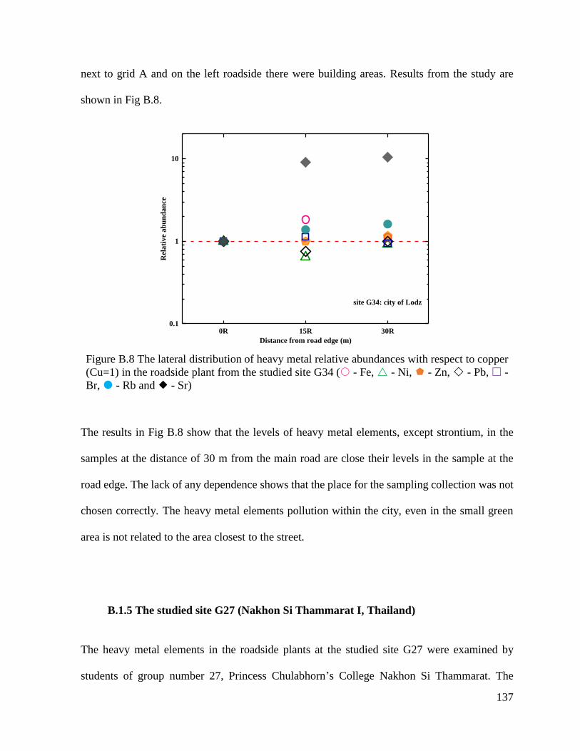
137

next to grid A and on the left roadside there were building areas. Results from the study are

shown in Fig B.8.

0R 15R 30R0.1

1

10R

ela

tiv

e a

bu

nd

an

ce


site G34: city of Lodz


(Cu=1) in the roadside plant from the studied site G34 ( - Fe, - Ni, - Zn, - Pb, -

Br, - Rb and - Sr)

The results in Fig B.8 show that the levels of heavy metal elements, except strontium, in the

samples at the distance of 30 m from the main road are close their levels in the sample at the

road edge. The lack of any dependence shows that the place for the sampling collection was not

chosen correctly. The heavy metal elements pollution within the city, even in the small green

area is not related to the area closest to the street.

B.1.5 The studied site G27 (Nakhon Si Thammarat I, Thailand)

The heavy metal elements in the roadside plants at the studied site G27 were examined by

students of group number 27, Princess Chulabhorn’s College Nakhon Si Thammarat. The

138

studied site is 40 km from their school. In Fig B.9, it is located on Thungsong – Nakhon Si

Thammarat road, part of Thailand route 403, in Ron Phibun district. This road links the city of

Nakhon Si Thammarat with Asian Highway 2 which is the main road for lower southern

provinces of Thailand. The road 403 was constructed over 50 years ago and upgraded from a

two-lane to a four-lane road in last ten years. It is used by all categories of vehicles. The traffic

rate on this road was 50,000 units per day.

(a)

(b)



collected (no sample is available on the research areas 25AR, 25BR, 50AR, 50BR and 50CR).

139

The plant samples of the Siam weed and tridax daisy were collected in the summer 2014, from

the fields, see Fig B.9 (a) and (b). These fields were covered by tall grass (over 30 cm) and some

parts on the right roadside constituted a wetland. Around the studied site, a few houses are

located out of the radius 100 m. There was not any barrier between the road and the studied site.

Results are shown in Fig B.10.


0.1

1

10

site G27: Nakhon Si. I

Rel

ati

ve

ab

un

da

nce





On the right roadside, the levels of heavy metal elements in the samples at the road edge and

at the distance of 25 m from the road edge are relatively similar and no systematics is observed.

On the left roadside, the majority of heavy metal elements show their declining relative

abundances in the samples aside the road edge. The high rate of decline can be observed in the

140

case of iron. Its relative abundance in the samples at the distance of 50 m from the road edge is

two times smaller than its level in the samples at the road edge. Generally, the relative abundance

of the heavy metal elements in the samples on the left roadside is relatively higher than in the

samples on the right roadside.

B.1.6 The studied site G28 (Nakhon Si Thammarat II, Thailand)

The heavy metal elements in the roadside plants at the studied site G28 were examined

by the students of group number 28, Princess Chulabhorn’s College Nakhon Si Thammarat. The

studied site is 16 km from their school. In Fig B.11, it is located on Thungsong – Nakhon Si

Thammarat road, in Maung district. The site G27 is on the same road with the studied site G28.

The site G27 is 24 km far from the site G28 in the inbound direction. The geographical feature

and traffic rate of the two studied sites were still relatively close.

(a)


99.9288888), and (b) shows the site plan with the areas (green blocks) where the samples

were collected (no sample is collected from the research areas 0AR, 25AR, 25BR, 25CR,

50AR, 50BR, 50CR, 25AL, 25CL, 50AL, 50BL and 50CL).

141

(b)


The plant samples of the Siam weed and tridax daisy were collected in the summer 2014, from

the fields, see Fig B.11 (a). The fields were covered by tall grass (over 30 cm) and some parts

on the right and left roadside constituted a wetland. Next to grid AR there was a private road of

a school. Results are shown in Fig B.12.

142


0.1

1

10

site G28: Nakhon Si. II

Rel

ati

ve

ab

un

da

nce





The number of measured points and lack of data for the longer distances makes this graph

inconclusive, but it can be combined with the data shown by the previous Thai group, G27.

143

B.2 Dispersion of relative abundances of heavy metal elements in the

roadside plants of the studied sites in Thailand

0 1 2 3 4 50

2

4

6

Fre

qu

ency

Relative abundance

Model Gauss

Equationy=y0 + (A/(w*sqrt(PI/2)))*exp(-2*((x-

xc)/w)^2)

Reduced

Chi-Sqr

0.64832

Adj. R-Square 0.83497

Value Standard Error

J

y0 0 0

xc 2 0

w 1.51143 0.1876

A 9.5 0

sigma 0.75571 0.0938

FWHM 1.77957 0.22088

Height 5.01506 0.62247

Fe

x = 2

= 0.8

(a)

0.0 0.2 0.4 0.6 0.8 1.0 1.2 1.40

1

2

3

4

Fre

qu

ency

Relative abundance

Ni

x = 0.7

= 0.2

(b)

0.0 0.5 1.0 1.5 2.0 2.5 3.00

2

4

6

Fre

qu

ency

Relative abundance

Zn

x = 1.1

= 0.5

(c)

0.0 0.5 1.0 1.5 2.00

1

2

3

Fre

qu

ency

Relative abundance

Pb

x = 1.0

= 0.28

(d)

Figure B.13 Histograms showing the distributions of (a) iron, (b) nickel, (c) zinc, (d) lead, (e)

bromine, (f) rubidium and (f) strontium in the samples of Thailand. The parameters are listed:

x – average and - dispersion

144

0 1 2 3 4 5 6 70

2

4

6

Fre

qu

ency

Relative abundance

Br

x = 1.9

= 0.6

(e)

0 2 4 6 8 10 12 14 160

1

2

3

4

Fre

qu

ency

Relative abundance

Rb

x = 8.1

= 2.5

(f)

0 2 4 6 8 10 12 14 160

1

2

3

4

5

Fre

qu

ency

Relative abundance

Sr

x = 8.6

= 2.5

(g)


145

Literature cited

Agunbiade, F. O., and A. T. Fawale, “Use of Siam Weed Biomarker in Assessing Heavy Metal

Contaminations in Traffic and Solid Waste Polluted Areas”, International Journal

of Environmental Science and Technology, vol. 6, no. 2, 2009, pp. 267 – 276.

Alloway, B. J., Zinc in Soils and Crop Nutrition, Brussels and Paris, IZA and IFA, 2008.

Alov, N. V., R. V. Bulgachev, and K. V. Oskolok, “Features of Technogenic Metal Pollution

of Roadside Soil According to X-Ray Fluorescence Monitoring Data”, Journal of Soils

and Sediments, vol. 1, no. 3, 2001, pp. 164 – 167.

Atafar, Z., et al., “Effect of Fertilizer Application on Soil Heavy Metal Concentration”,

Environmental Monitoring and Assessment, vol. 160, no. 1 – 4, 2010, pp. 83 – 89.

Atiemo, S. M., et al., “Levels and Sources of Heavy Metal Concentration in Road Dust in

Selected Major Highways of Accra, Ghana”, X-ray Spectrometry, vol. 41, no. 2, 2012, pp.

105 – 110.

Bendtsen, H., Noise Barrier Design, Danish and Some European Examples Report 174, Road

Directorate, Danish Road Institute, 2009, p. 13.

Bennet, C., P. Jonsson, and E. S. Lindgren, “Concentrations and Sources of Trace Elements

in Particulate Air Pollution, Dar Es Salaam, Tanzania, studied by EDXRF”, X-ray

Spectrometry, vol. 34, no. 1, 2005, pp. 1 – 6.

Bolin, B., et al. (eds.), The Greenhouse Effect, Climatic Change, and Ecosystems, New York,

John Wiley and Sons, 1986.

146

Bruker AXS Microanalysis GmbH, S2 PICOFOXtm User Manual, Berlin, Bruker AXS

Microanalysis GmbH, 2008.

Capannesi, G., et al., “Feasibility of Oak Leaves as Monitor for Airborne Pollution”, Journal

of Radioanalytical and Nuclear Chemistry, vol. 167, no. 2, 1993, pp. 309 – 320.

Cheung, K. L., et al., “Emissions of Particulate Trace Elements, Metals and Organic Species

from Gasoline, Diesel, and Biodiesel Passenger Vehicles and Their Relation to Oxidative

Potential”, Aerosol Science and Technology, vol. 44, no. 7, 2010, pp. 500 – 513.

Daines, R. H., H. Motto, and D. M. Chilko, “Atmospheric Lead: Its Relationship to Traffic

Volume and Proximity to Highways”, Environmental Science and Technology, vol. 4, no.

4, 1970, pp. 318 – 322.

Damilola, F. H., and O. A. Morenikeji, “Heavy Metals in Soils, Ash and Tridax procumbens

in the Vicinity of the University College Hospital Incinerator in Ibadan, South-West,

Nigeria”, Journal of Science Research, vol. 12, 2013, pp. 135 – 144.

Degobert, P., Automobiles and Pollution, Paris, Editions Technip, 1992.

Djingova, R., and I. Kuleff, “Bromine, Copper, Manganese and Lead Content of the Leaves

of Taraxacum officinale (Dandelion)”, Science of the Total Environment, vol. 50, 1986,

pp. 197 – 208.

Dudka, S., et al., “Trace Metal Contamination of Soils and Crop Plants by the Mining

and Smelting Industry in Upper Silesia, South Poland”, Journal of Geochemical

Exploration, vol. 52, no. 1, 1995, pp. 237 – 250.

147

Eck, D. J., ScatterPlotApplet, New York, Department of Mathematics and Computer Science,

Hobart and William Smith Colleges, 2012.

Fosmire, G. J., “Zinc Toxicity”, American Journal of Clinical Nutrition, vol. 51, no. 2, 1990,

pp. 225 – 227.

Franzoni, C., and H. Sauermann, “Crowd Science: the Organization of Scientific Research

in Open Collaborative Projects”, Research Policy, vol. 43, no. 1, 2014, pp. 1 – 20.

Garcia, R., and E. Millan, “Assessment of Cd, Pb and Zn Contamination in Roadside Soils

and Grasses from Gipuzkoa (Spain)”, Chemosphere, vol. 37, no. 8, 1998, pp. 1615 – 1625.

Gift, J., et al., Toxicological Review of 1,2-Dibromoethane, Washington, DC, U.S.

Environmental Protection Agency, 2004.

Grigalaviciene, I., V. Rutkoviene, and V. Marozas, “The Accumulation of Heavy Metals Pb, Cu

and Cd at Roadside Forest Soil”, Polish Journal of Environmental Studies, vol. 14, no. 1,

2005, pp. 109 – 115.

Groysman, A., Corrosion in Systems for Storage and Transportation of Petroleum Products

and Biofuels, Identification, Monitoring and Solutions, Dordrecht, Springer Netherlands,

2014.

Hallet, J. Ph., et al., “Elemental Deposition as a Function of Distance from an Industrial Zone”,

Science of the Total Environment, vol. 25, no. 2, 1982, pp. 99 – 109.

Hamilton, R. S., and R. M. Harrison (eds.), Highway pollution, The Netherlands, Elsevier

Science Publishers, 1991.

148

Harrison, R. M., D. P. H. Laxen, and S. J. Wilson, “Chemical Associations of Lead, Cadmium,

Copper, and Zinc in Street Dusts and Roadside Soils”, Environmental Science

and Technology, vol. 15, no. 11, 1981, pp. 1378 – 1383.

Hjortenkrans, D. S. T., B. G. Bergback, and A. V. Haggerud, “Metal Emissions from Brake

Linings and Tires: Case Studies of Stockholm, Sweden 1995/1998 and 2005,

Environmental Science and Technology, vol. 41, no. 15, 2007, pp. 5224 – 5230.

Ikewuchi, J. C., and C. C. Ikewuchi, “Comparative Study of the Mineral Element Composition

of Some Common Nigerian Medical Plants”, Pacific Journal of Science

and Technology, vol. 10, no. 1, 2009, pp. 362 – 366.

Johnsen, I., K. Pilegaard, and E. Nymand, “Heavy Metal Uptake in Transplanted and In Situ

Yarrow (Achillea millefolium) and Epiphytic Cryptogams at Rural, Urban and Industrial

Localities in Denmark”, Environmental Monitoring and Assessment, vol. 3, no. 1, 1983,

pp. 13 – 22.

Jungers, R. H., R. E. Lee, Jr, and D. J. V. Lehmden, “The EPA National Fuels Surveillance

Network. I. Trace Constituents in Gasoline and Commercial Gasoline Fuel Additives”,

Environmental Health Perspectives, vol. 10, 1975, pp. 143 – 150.

Kozanecka, T., et al., “Content of Microelements in Selected Herbs from Natural Meadows”,

Polish Journal of Environmental Studies, vol. 15, no. 2a, 2006, pp. 385 – 389.

Kabata-Pendias, A., and S. Dudka, “Trace Metal Contents of Taraxacum officinale (Dadelion)

as a Convenient Environmental Indicator”, Environmental Geochemistry and Health, vol.

13, no. 2, 1991, pp. 108 – 113.

149

Królak, E., “Accumulation of Zn, Cu, Pb and Cd by Dandelion (Taraxacum officinale Web.)

in Environments with Various Degrees of Metallic Contamination”, Polish Journal

of Environmental Studies, vol. 12, no. 6, 2003, pp. 713 – 721.

Krzyzanowski, M., B. Kuna-Dibbert, and J. Schneider (eds.), Health Effects of Transport-

Related Air Pollution, Denmark, World Health Organization, 2005.

Lagerwerff, J. V., and A. W. Specht, “Contamination of Roadside Soil and Vegetation

with Cadmium, Nickel, Lead, and Zinc”, Environmental Science and Technology, vol. 4,

no. 7, 1970, pp. 583 – 586.

Lammel, G., A. Rohrl, and H. Schreiber, “Atmospheric Lead and Bromine in Germany, Post-

Abatement Levels, Variabilities and Trends”, Environmental Science and Pollution

Research, vol. 9, no. 6, 2002, pp. 397 – 404.

Legret, M., and C. Pagotto, “Heavy Metal Deposition and Soil Pollution Along Two Major

Rural Highways”, Environmental Technology, vol. 27, no. 3, 2006, pp. 247 – 254.

Lepp, N. W. (ed.), Effect of Heavy Metal Pollution on Plants, London and New Jersey, Applied

Science Publishers, 1981.

Ligocki, M., et al., “The Common Dandelion (Taraxacum officinale) as an Indicator

of Anthropogenic Toxic Metal Pollution of Environment”, Acta Scientiarum Polonorum,

Zootechnica, vol. 10, no. 4, 2011, pp. 73 – 82.

Luhana, L., et al., Measurement of Non-Exhaust Particulate Matter, European Commission –

DG TrEn, 5th Framework Programme, Competitive and Sustainable Growth, Sustainable

Mobility and Intermodality, 2004, pp. 9 – 12.

150

Medicinal herbs, (n. d.), Achillea millefolium, [online photograph], http://www.blumenboom.

ru/ru/catalog/medicinal_herbs/42/1, (accessed 5 October 2015).

Medicinal herbs, (n. d.), Tridax procumbens L., [online photograph], http://www.mpbd.info/

plants/ tridax-procumbens.php, (accessed 5 October 2015).

Medicinal herbs, (n. d.), Siam weed, [online photograph], http://www.samunpri.com/?p=6132,

(accessed 5 October 2015).

Mortvedt, J. J., “Heavy Metal Contaminants in Inorganic and Organic Fertilizers”, Fertilizer

Research, vol. 43, no. 1, 1995, pp. 55 – 61.

Murphy, C., and J. Beggs, Primary Science in the UK: a Scoping Study, London, Wellcome

Trust, 2005, p. 12.

Nriagu, J. O., “The Rise and Fall of Leaded Gasoline”, Science of the Total Environment,

vol. 92, 1990, pp. 13 – 28.

Oblad, M., and E. Selin, “Measurements of Br/Pb Ratios in Airborne Particles from Car

Exhaust”, Physica Scripta, vol. 32, no. 4, 1985, pp. 462 – 468.

Othman, I., M. Al-Oudat, and M. S. Al-Masri, “Lead Levels in Roadside Soils and Vegetation

of Damascus City”, Science of the Total Environment, vol. 207, no. 1, 1997, pp. 43 – 48.

Pell, T., and T. Jarvis, “Developing Attitude to Science Scales for Use with Children of Ages

from Five to Eleven Years”, International Journal of Science Education, vol. 23, no. 8,

2001, pp. 847 – 862.

Prasad, M. N. V., K. S. Sajwan, and R. Naidu (eds.), “Trace Elements in the Environment:

Biogeochemistry, Biotechnology and Bioremediation”, Florida, CRC Press, 2006.

151

Ribeiro, K. S., et al., “Transport and Its Infrastructure. In Climate Change 2007: Mitigation.

Contribution of Working Group III to the Fourth Assessment Report of the

Intergovernmental Panel on Climate Change”, in B. Metz, et al. (eds.), Cambridge, United

Kingdom and New York, Cambridge University Press, 2007.

Schuck, E. A., and J. K. Locke, “Relationship of Automotive Lead Particulates to Certain

Consumer Crops”, Environmental Science and Technology, vol. 4, no. 4, 1970, pp. 324 –

330.

Sezgin, N., et al., “Determination of Heavy Metal Concentrations in Street Dusts in Istanbul E-

5 Highway”, Environment International, vol. 29, no. 7, 2003, pp. 979 – 985.

Skinner, E. R., Jr., “Highway Design and Construction: the Innovation Challenge”, The Bridge,

vol. 38, no. 2, Summer 2008, pp. 5 – 12.

Smithers, A., and P. Robinson, The Growth of Mixed A-Levels, Manchester, Carmichael Press,

1988.

Szymański, M., et al., “Effects of Trace Elements on Polyphenolic Compounds in Millefolii

Herba”, Polish Journal of Environmental Studies, vol. 23, no. 2, 2014, pp. 459 – 466.

Szynkowska, M. I., et al., “Toxic Metal Distribution in Rural and Urban Soil Samples Affected

by Industry and Traffic”, Polish Journal of Environmental Studies, vol. 18, no. 6, 2009,

pp. 1141 – 1150.

Swietlicki, E., and R. Krejci, “Source Characterisation of the Central European Atmospheric

Aerosol Using Multivariate Statistical Methods”, Nuclear Instruments and Methods

in Physics Research Section B, Beam Interactions with Materials and Atoms, vol. 109/110,

1996, pp. 519 – 525.

152

Tanhan, P., et al., “Uptake and Accumulation of Cadmium, Lead and Zinc by Siam Weed

[Chromolaena odorata (L.) King & Robinson]”, Chemosphere, vol. 68, no. 2, 2007, pp.

323 – 329.

Thomas, V. M., J. A. Bedford, and R. J. Cicerone, “Bromine Emissions from Leaded Gasoline”,

Geophysical Research Letters, vol. 24, no. 11, 1997, pp. 1371 – 1374.

Viard, B., et al., “Integrated Assessment of Heavy Metal (Pb, Zn, Cd) Highway Pollution:

Bioaccumulation in Soil, Graminaceae and Land Snails”, Chemosphere, vol. 55, no. 10,

2004, pp. 1349 – 1359.

Ward, N. I., et al., “Heavy-Metal Pollution from Automotive Emissions and Its Effect on

Roadside Soils and Pasture Species in New Zealand”, Environmental Science and

Technology, vol. 11, no. 9, 1977, pp. 917 – 920.

Williams, M., et al., “Arsenic Contamination in Surface Drainage and Groundwater in Part

of the Southeast Asian Tin Belt, Nakhon Si Thammarat Province, Southern Thailand”,

Environmental Geology, vol. 27, no. 1, 1996, pp. 16 – 33.

Wong, J. W. C., and N. K. Mak, “Heavy Metal Pollution in Children Playgrounds in Hong Kong

and Its Health Implications”, Environmental Technology, vol. 18, no. 1, 1997, pp. 109 –

115.

Zakir, H. M., N. Sultana, and M. Akter, “Heavy Metal Contamination in Roadside Soils

and Grasses: a Case Study from Dhaka City, Bangladesh”, Journal of Chemical,

Biological and Physical Sciences, vol. 4. No. 2, 2014, pp. 1661 – 1673.

153

Zhang, F., et al., “Influence of Traffic Activity on Heavy Metal Concentrations of Roadside

Farmland Soil in Mountainous Areas”, International Journal of Environmental Research

and Public Health, vol. 9, no. 5, 2012, pp. 1715 – 1731.

Zhao, H., B. Cui, and K. Zhang, “The Distribution of Heavy Metal in Surface Soils and Their

Uptake by Plants Along Roadside Slopes in Longitudinal Range Gorge Region, China”,

Environmental Earth Sciences, vol. 61, no. 5, 2010, pp. 1013 – 1023.

Zimdahl, R. L., and J. J. Hassett, “Lead in Soil”, in W. R. Boggess (ed.), Lead in the

Environment, National Science Foundation, Washington, DC., 1977, pp. 93 – 98.

154

ACKNOWLEDGEMENTS

I sincerely thank my advisor prof. dr hab. Tadeusz Wibig for his extraordinary support, advice

and help throughout my study.

I would like to thank dr. Aldona Kubala-Kukuś, mgr Ilona Stabrawa and colleagues at the X-

ray Spectrometry Laboratory, Jan Kochanowski University in Kielce for imparting me the

knowledge about measuring techniques using different types of X-ray spectrometers and

providing me with the excellent TXRF spectrometer for measurement of all samples in the

research. I also thank to dr. Józef Krawczyk, dr. Joanna Łubocka, dr. Agnieszka Klink, mgr

Ludmiła Polechońska and the colleagues at the Faculty of Biological Science, University of

Wrocław for their expert advice about biology and environmental science throughout this

research process.

My study would have been impossible without the support and grant permission of the Ministry

of Science and Technology, Walailak University in Thailand, as well as University of Łódź in

Poland.

Thanks to the support, help and encouragement of assist prof. dr. Mudtorlep Nisoa, assoc prof.

dr. Chitnarong Sirisathitkul and assist prof. dr. Sorasak Danworapong – my teachers at Walailak

University; and dr. Jadwiga Skurska, pani Elżbieta Osetek, dr. Piotr Skurski and dr. Paweł

Barczyński – my colleagues at University of Łódź.

Finally, I could not have got through this endeavour without the love and support of my dear

family and friends through these past years. Thank you so much.

155

BIOGRAPHY SKETCH

Punsiri Dam-o was born in Nakhon Si Thammarat, Thailand in 1981 and was raised by her

parents: Nuhein and Paur, with her elder sister and brothers: Wissawan, Chalermpol and Pinij.

When growing up, she gained a good appreciation for the natural world through going on forest,

mountain and sea trips with her late father*. Her interest in science began back in High School

at the Princess Chulabhorn’s College Nakhon Si Thammarat (PCC NST), where she became

involved in various scientific activities. These included conducting an Environmental

Conservation Club. It was there she found herself enjoy teaching her friends in physics, with

the advice and guidance of her teacher: Suwanij Julawat. From there Punsiri then decided to

attend the Physics Education Program at the Prince of Songkhla University (PSU), Pattani

Campus. She went on to spend the summer of her senior year teaching physics to pupils in

Southern Thailand. She graduated from PSU with a B.Sc. degree in Physics Education with

honors back in 2002. On graduation she started her career as a physics teacher at PCC NST.

After teaching at the school for one year, she then decided to leave there to continue her own

education, enrolling on the M. Sc. degree in Physics Studies at Walailak University (WU). Once

there Punsiri worked in the lab of dr. Ketsiri Kueseng** and assist prof. dr. Kowit

Kittiwutthisakdi as a graduate student, working in the field of development of atomic and

molecular modeling as part of the fundamental science curriculum. This included studying the

properties and behaviours of water molecules and also the development of physical models of

functional groups in molecules. After obtaining the M.Sc. degree, she worked as a physics

lecturer at the university (WU) for a number of years and was then promoted to be a Ph.D.

degree scholarship recipient. The Ph.D. degree scholarship is awarded by the Ministry of

156

Science and Technology in Thailand. Having received the scholarship she then moved to Poland

to study physics at University of Łódź and worked in the lab of prof. dr hab. Tadeusz Wibig, as

a doctoral student in the field of remote laboratories for educational physics: interactive wind

tunnel and x-ray spectroscopy labs, from the fall of 2009.

*,** In loving memory of both my late father and my ex-advisor who very sadly passed away

Examination of Some Heavy Metal Pollution in Roadside ...

Documents