Exact solutions of anisotropic diffusion-limited reactions with coagulation and annihilation

arX

iv:c

ond-

mat

/950

3064

v1 1

2 M

ar 1

995

Exact Solutions of Anisotropic Diffusion-Limited

Reactions with Coagulation and Annihilation

Vladimir Privman, Antonio M. R. Cadilhe, and M. Lawrence Glasser

Department of Physics, Clarkson University, Potsdam, New York 13699–5820, USA

ABSTRACT

We report exact results for one-dimensional reaction-diffusion models A + A →

inert, A + A → A, and A + B → inert, where in the latter case like particles coagulate

on encounters and move as clusters. Our study emphasized anisotropy of hopping

rates; no changes in universal properties were found, due to anisotropy, in all three

reactions. The method of solution employed mapping onto a model of coagulating

positive integer charges. The dynamical rules were synchronous, cellular-automaton

type. All the asymptotic large-time results for particle densities were consistent, in the

framework of universality, with other model results with different dynamical rules, when

available in the literature.

PACS numbers: 05.40.+j, 82.20.-w

KEY words: reactions, anisotropic diffusion, coagulation, synchronous dynamics

Running title: Anisotropic diffusion-limited reactions

– 1 –

I. INTRODUCTION

Diffusion-Limited Reactions (DLR) involving aggregation and annihilation pro-

cesses are important in many physical, chemical and biological phenomena [1-3] such

as star formation, polymerization, recombination of charge carriers in semiconductors,

soliton and antisoliton annihilation, biologically competing species, etc. In this paper

we generalize and apply a recently introduced method [4-5], in order to study by exact

solution effects of anisotropy in some common DLR in one dimension (1D), specifically,

A + A → A, A + A → inert, and a two-species annihilation model A + B → inert in

which like particles coagulate irreversibly. The detailed definitions will be given later.

Scaling approaches and other methods have yielded [1-3,6-12] the upper critical

dimension, Dc, for various reactions. Typical values range from 2 to 4. For spatial

dimensions lower than Dc the kinetics of these reactions is fluctuation-dominated, and

we cannot expect the rate equation approach to be valid. Indeed the mean-field rate

equation approximation ignores effects of inhomogeneous fluctuations. Fluctuation-

dominated DLR have been subject to numerous studies by other methods, notably,

exact solutions and asymptotic arguments [1,13-22] in 1D. The 1D reactions have also

found some experimental applications [23-24]. These studies have assumed isotropic

hopping (reactant particle diffusion).

Recently Janowsky [25] concluded, based on numerical results and phenomenologi-

cal considerations for the two species annihilation reaction A + B → inert, that making

the hopping fully directed would change the universality class in 1D. Specifically, the

large-time particle concentration (assuming equal densities of both species), would scale

according to c(t) ∼ t−1/3 instead of the isotropic-hopping power law t−1/4. A few exact

and numerical results available in the literature on anisotropic reactions involving only

– 2 –

one species [26-27] indicate that the power law is not changed. The model of [25] as-

sumed that like particles interact via hard-core repulsion; this seems to be an essential

ingredient for observing the changeover in the universality class.

In this work we report the exact solution for two-particle annihilation with anisotropic

hopping. We consider discrete-time simultaneous-updating dynamics, also termed syn-

chronous dynamics, so that our models are cellular-automaton type. The universality

classes of behavior at large times and large spatial scales are expected not to depend

on details of the model dynamics. However, in order to achieve exact solvability we

took “sticky-particle” rather than hard-core interactions: the like particles coagulate

on encounters and diffuse as groups. Our exact calculations yield the t−1/4 power law,

found earlier for similar “sticky-particle” reactions with isotropic hopping [28-29]. This

result is probably due to absence of hard-core interactions in our model.

For unequal initial concentrations, the large-time behavior changes, see [28-29]. The

crossover between the two regimes is derived analytically. Finally, we also obtain new

exact results for single-species two-particle aggregation and annihilation reactions with

anisotropy; see also [26]. We find that anisotropy does not change the universality class

of kinetics of these reactions. A short version of this work was reported in a letter-style

publication [30].

This paper is organized as follows: in Section II we define and review some existing

results for the models studied. In Section III our method for exact solution is introduced.

In section IV, results for the single-species models are presented. Finally, Section V is

devoted to the two-species model. Further scaling analysis of the two-species model and

the brief summarizing discussion are left to Section VI.

– 3 –

II. REACTION-DIFFUSION MODELS

In lattice DLR models with like particles it is usually assumed that the particles

hop independently, to the extent allowed by their interactions, to their nearest neighbor

sites. Whenever two particles meet, they can both annihilate which corresponds to the

reaction A + A → inert. If, however, only one particle of a pair disappears we get the

reaction A + A → A usually termed “aggregation.” Such single-species reactions have

the upper critical dimension Dc = 2 [6-9]. For D < 2 the particle concentration at large

times behaves according to c(t) ∼ t−D/2. Specifically, the 1D kinetics of these reactions

is non-mean-field, with the typical diffusional behavior c(t) ∼ t−1/2. This result is not

affected by short-range interactions between the particles and is not sensitive to their

initial distribution as long as initial correlations are sufficiently short-range.

Consider now the two-particle annihilation model, to be termed the AB model.

Particles hop randomly to one of their nearest-neighbor sites. Whenever two parti-

cles meet, unlike species annihilate, A + B → inert. When like species meet, some

interaction must be assumed. The simplest interaction is hard-core: diffusion attempts

leading to multiple occupancy of lattice sites are discarded. For such reactions, assum-

ing equal average A- and B-concentrations and uniform initial conditions, the upper

critical dimension is Dc = 4 [6-9]. The (equal) particle concentrations scale according

to c(t) ∼ t−D/4. A surprising largely numerically-based recent result of Janowsky [25]

is the new exponent ≈ 1/3, replacing 1/4, for anisotropic particle hopping in 1D. For

unequal initial concentrations, the density of the minority species is expected to decay

faster than the symmetric-case power-law; some specific results will be referred to later.

In order to obtain a solvable model in 1D, let us now consider the AB annihilation

model with the “sticky particle” interaction. Thus, like particles coagulate irreversibly

– 4 –

on encounters, for instance,

nA + mA → (n + m)A , (2.1)

and the clusters thus formed then diffuse as single entities with the single-particle hop-

ping rates. When unlike clusters meet at a lattice site, the outcome of the reaction

is

nA + mB →

(n − m)A if n > minert if n = m(m − n)B if n < m

(2.2)

Recent numerical results and scaling considerations for these reactions [31] in D = 1, 2, 3

seem to suggest that they are mean-field in D = 2, 3. However, in 1D the power-law

exponent for the density is 1/4, obtained by exact solution [28-29] which also yielded a

faster power-law decay ∼ t−3/2 for the minority species in case of unequal densities of

A and B.

As mentioned earlier, in order to obtain exact solutions for our single-species and

AB models, we first solve another model [4], of coagulating nonnegative integer charges

in 1D [4-5], with anisotropic hopping. All our models are defined with synchronous

dynamics to be described in detail in the next section, along with detailed dynamical

rules and their exact solution. From the coagulating-charge model one can derive results

for the reactions A+A → A and A+A → inert with anisotropic hopping; see Section IV.

Some of our expressions are new, while other are consistent with results available in the

literature. We next use the approach of [28-29] to extend the coagulating-charge solution

to the “sticky” AB model. We find that hopping anisotropy does not change the density

exponent in 1D: it remains 1/4; see Section V.

– 5 –

III. SYNCHRONOUS DYNAMICS OF COAGULATING CHARGES

Let us consider a one-dimensional lattice with unit spacing. Following [4], we

consider diffusion of nonnegative charges on this lattice. Initially, at t = 0, we place

positive unit charge at each site with probability p or zero charge with probability

1 − p. Furthermore, we consider synchronous dynamics, i.e., charges at all lattice sites

hop simultaneously in each time step t → t + 1, where t = 0, 1, 2, . . .. However, the

probabilities of hopping to the right, r, and to the left, ℓ = 1 − r, are not necessarily

equal. Since this dynamics decouples the even-odd and odd-even space-time sublattices,

it suffices to consider only those charges which are at the even sublattice at t = 0. Thus

we only consider the lattice sites j = 0,±2,±4, . . . at times t = 0, 2, 4, . . ., and lattice

sites j = ±1,±3,±5, . . . at times t = 1, 3, 5, . . ..

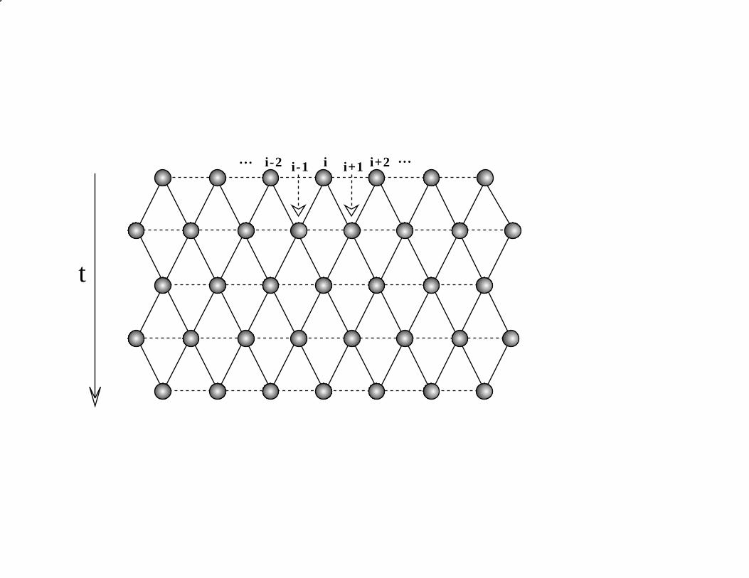
One can view the diffusional hopping as taking place on a directed square lattice

with the time direction along the “directed” diagonal. This lattice is illustrated in

Figure 1; note that the charges arriving at site j at time t can only come from the sites

j−1 and j +1 at time t−1. Finally, the “interaction” between the charges is defined by

the rule that all charge accumulated at site j at time t coagulates. There can be 0, 1 or

2 such charges arriving from the two nearest neighbors of j in the time step t − 1 → t,

depending on the random decisions regarding the directions of hopping from sites j ± 1

in this time step.

This model can also be viewed as diffusion-coagulation of unit-charge “particles”

C, where the coagulation is represented by the reaction

nC + mC → (n + m)C . (3.1)

Such reactions, without the limitation of positive or integer charges, and with an added

– 6 –

process of feeding-in charge at each time step, with values drawn randomly at each site

from some fixed distribution, have been considered as models of self-organized criticality

and coagulation [5,32-33]. These studies were limited to isotropic hopping, i.e., r = ℓ =

12. Our interest in these reactions is in that their dynamics can be mapped [4,28-29]

onto that of both the single-species (Section IV) and “sticky” AB (Section V) reaction-

diffusion models introduced in Section II. However, before discussing and utilizing this

mapping, let us present the exact solution of the model of coagulating charges with

anisotropic hopping, following the ideas of [4-5].

For each time t and at each lattice site j (of the relevant sublattice) we define

stochastic variables,

τj(t) =

1, probability r0, probability ℓ

(3.2)

which represent the hopping direction decisions. Then the stochastic equation of motion

for the charges qj(t), equal to the number of C particles at site j at time t, is

qn(t + 1) = τn−1(t)qn−1(t) + [1 − τn+1(t)] qn+1(t) . (3.3)

The total number of C-particles, or the total charge, in an interval of k consecutive

proper-parity-sublattice sites, starting at site j at time t, is given by

Sk,j(t) =

k−1∑

i=0

qj+2i(t) = qj(t) + qj+2(t) + · · ·+ +qi+2k−2(t) . (3.4)

Due to conservation of charge in this process, the equations of motion (3.3) yield the

following relation,

– 7 –

Sk,n(t + 1) = τn−1(t)qn−1(t)

+ qn+1(t) + · · ·+ qn+2k−3(t)

+ [1 − τn+2k−1(t)] qn+2k−1(t) . (3.5)

This result indicates that only the two random decisions at the end points are in-

volved in the dynamics of charges in consecutive-site intervals. The exact solvability

of coagulating-charge models is based on this property, as first observed in [5]. Other

solution methods were used in related interface-growth models [34] which will not be

discussed here.

Let us introduce the function

I(s, m) = δs,m , (3.6)

and averages,

fk,m(t) = 〈I (Sk,j(t), m)〉 . (3.7)

The average 〈· · ·〉 is over the stochastic dynamics, i.e., over random choices of the

decision variables τi(t), as well as over the random initial conditions. Since the latter

are uniform, the averages fk,m(t) in (3.7) do not depend on the lattice site j. Functions

other than the Kronecker delta have been used for I(s, m) in the literature [4-5,32-33].

With our choice (3.6), the resulting averages fk,m(t) correspond to the probability to

find exactly m charge units in an interval of k consecutive sites. For instance, f1,m(t)

is the density (fraction) of sites with charge m.

Note that (3.5) essentially represents the following simple rule: charge “fed” into

an interval of k sites comes from k + 1 sites, at the preceding time-variable value, with

– 8 –

probability rl, from k − 1 sites with probability rl, and from two possible groups of

k sites, with probabilities r2 and ℓ2; this is illustrated in Figure 2. Furthermore, the

variables τi(t) and Sk,n(t) are statistically independent because the latter only depends

on “decision making” variables τi at earlier times. Therefore, the averages introduced

in (3.7) satisfy, for any function I(s, m), the following equations of motion,

fk,m(t + 1) = rℓ [fk+1,m(t) + fk−1,m(t)] +(

r2 + ℓ2)

fk,m(t) . (3.8)

Interestingly, the m-dependence is parametric in (3.8). However, it does enter the

initial conditions. It is also convenient [4] to define f0,m(t) = I(0, m) in order to extend

the applicability of (3.8) to all t ≥ 0. For our specific choices, we have the following

expressions. Firstly, the initial conditions of placing charges 1 or 0 at each site, with

respective probabilities p and 1 − p, correspond to

fk,m(0) =

pm(1 − p)k−m(

km

)

0 ≤ m ≤ k

0 m > k(3.9)

where(

km

)

= k!/ (m!(k − m)!). Secondly, the boundary condition is that a null interval

cannot have charges, i.e.,

f0,m(t ≥ 0) = δ0,m . (3.10)

In order to solve the equations of motion (3.8) we introduce the double generating

function of fk,m(t), over the time variable t and over the number of charges m, with

fixed number of sites k,

gk(u, w) =

∞∑

t=0

∞∑

m=0

fk,m(t)utwm . (3.11)

– 9 –

It is also convenient to introduce the variable a = r − ℓ directly measuring the hopping

anisotropy,

r = (1 + a)/2 and ℓ = (1 − a)/2 . (3.12)

A straightforward but tedious calculation then yields the following difference equation

which derives from the equations of motion (3.8), with(3.9),

gk+1(u, w)+2

(

1 + a2)

u − 2

(1 − a2)ugk(u, w)+gk−1(u, w) = − 4

(1 − a2)u(wp+1−p)k . (3.13)

The initial and boundary conditions “translate” as follows,

gk(0, w) = (wp + 1 − p)k , (3.14)

g0(u, w) =1

1 − u. (3.15)

The solution of (3.13) is obtained as a linear combination of the special solution

Ω(wp+1−p)k proportional to the right-hand side, and that solution of the homogeneous

equation which is regular at u = 0. The coefficient Ω is obtained by substitution,

Ω = − 4(wp + 1 − p)

(1 − a2)u (wp + 1 − p − Λ+) (wp + 1 − p − Λ−), (3.16)

where it is convenient to express the denominator in terms of the roots Λ± of the

characteristic equation of (3.13),

Λ2 + 2

(

1 + a2)

u − 2

(1 − a2) uΛ + 1 = 0 . (3.17)

– 10 –

These roots are given by

Λ± =2 −

(

1 + a2)

u ± 2√

(1 − u) (1 − a2u)

(1 − a2)u, (3.18)

and the root Λ−, which is nonsingular as u → 0, also gives the homogeneous solution

proportional to Λk−. The proportionality constant is determined by (3.15). In summary,

the solution takes the form

gk(u, w) =

(

1

1 − u− Ω

)

Λk− + Ω(wp + 1 − p)k . (3.19)

The w-dependence of this result is via Ω, see (3.16), and it is of a simple rational

form. Therefore, derivation of the dependence on the number of charges, “generated”

by w, is relatively simple. In our applications we will concentrate on densities of re-

actants at single lattice sites, derived from fk=1,m(t). The m-dependence then follows

by expanding (3.19) in powers of w. However, the u-dependence of (3.19) with (3.16),

(3.18), is more complicated. Therefore we will use the generating functions for the

time-dependence and most of our explicit time-dependent expressions will be derived

as asymptotic results valid for large times. Indeed, the power series in u are then con-

trolled by the singularity at u = 1, and analytical results can be derived by appropriate

expansions. Specifically, let us introduce the time-generating function for the quantities

f1,m(t) which represent the probability to find charge m at a lattice site at time t. We

define

Gm(u) =∞∑

t=0

f1,m(t)ut . (3.20)

The central result of this section is thus

– 11 –

Gm(u) = δm,0

[

Λ−

1 − u− 4

(1 − a2)u

]

− (−1)m 4Λ+pm

(1 − a2)u (1 − p − Λ+)m+1 , (3.21)

where Λ± were given in (3.18). Note that Gm(u) is just the mth Taylor series coefficient

in w, of the function g1(u, w).

– 12 –

IV. SINGLE-SPECIES REACTIONS

In this section we map the coagulating-charge model onto the two single-species

reactions introduced in Section II. This approach follows recent work [4], although re-

lated ideas have been used in earlier literature, for instance, in [35]. Let us consider

first the two-particle aggregation reaction A+A → A. In the coagulating-charge model

we now regard each “charged” site as occupied by an A-particle, and each “uncharged”

site as empty of A-particles. Specifically, any charge m > 0 represents an A particle.

No charge at a site, m = 0, corresponds to absence of an A particle. The dynamics of

the coagulating charges then maps onto the dynamics of the reaction A+A → A on the

same lattice, with the initial conditions of placing particles A randomly with probability

p, or leaving the lattice sites vacant with probability 1− p, so that the initial density of

the A particles is

c(0) = p . (4.1)

We now observe that the quantity f1,0(t) gives the density of empty sites in both

models. Therefore, the particle density (per lattice site), c(t), in the aggregation model,

is given by

c(t) = 1 − f1,0(t) . (4.2)

The generating function is therefore easily derivable from (3.21),

E(u) =

∞∑

t=0

c(t)ut =1

1 − u− G0(u) =

1 − Λ−

1 − u+

4(1 − p)

(1 − a2)u (1 − p − Λ+). (4.3)

– 13 –

The function E(u) is actually regular at u = 0. Thus the Taylor series is controlled

by the singularity at u = 1, near which we have the leading-order term

E(u) =2√

1 − a2

[

1√1 − u

+ O(1)

]

. (4.4)

This yields the leading-order large-time behavior,

c(t) ≈ 2√

(1 − a2)πt. (4.5)

While we are not aware of other exact solutions for this model with anisotropic hopping,

the result (4.5) is not surprising. Indeed, the leading-order large time behavior is ex-

pected to be universal in that it does not depend on the initial density p. Furthermore,

the diffusion constant D(a) =(

1 − a2)

D(0) decreases proportional to 1 − a2 when the

anisotropy is introduced (single-particle diffusion is then of course also accompanied by

drift). Therefore, as a function of D(a)t, the result (4.5) also does not depend on the

anisotropy and in fact it is the same as expressions found for other A+A → A reaction

models, with different detailed dynamical rules (with isotropic hopping), e.g., [20].

Let us now turn to the two-particle annihilation model A +A → inert. The appro-

priate mapping here is to identify odd charges with particles A and even charges with

empty sites. Indeed, the dynamics of the coagulating-charge model is then mapped onto

the reaction A + A → inert. Thus, each lattice site with an odd charge q = 1, 3, 5, . . .

will be replaced by a site with one A particle. Each lattice site with an even charge

q = 0, 2, 4, . . . is empty of A-particles. The rules of charge coagulation then reduce

to the desired reaction. Furthermore, relation (4.1) applies. However, the generating

function E(u) for particle density is given by a different expression,

– 14 –

E(u) =

∞∑

j=0

G2j+1(u) =4Λ+p

(1 − a2)u[

(1 − p − Λ+)2 − p2

] . (4.6)

The large-time behavior is similar to the aggregation reaction, with the universal ex-

pression which only differs from (4.5) by a factor of 2,

c(t) ≈ 1√

(1 − a2)πt. (4.7)

While the large-time behavior of both models is model-independent and otherwise

universal as described earlier, the finite-time results do depend on details of the dynam-

ical rules. For our particular choice of synchronous dynamics on alternating sublattices

(Figure 1), there exists an exact mapping relating the isotropic-hopping aggregation

and annihilation reactions [4]. This mapping was also found for the anisotropic-hopping

results obtained here. Specifically, we find (by comparing their generating functions)

2cinert(t; p) = cA(t; 2p) , (4.8)

where the subscripts denote the outcome of the reaction while the added argument

stands for the initial density. Thus if we consider an annihilation reaction with, initially,

at t = 0, half the particle density as compared to an aggregation reaction with the same

synchronous dynamical rules, then the density ratio will remain exactly 1/2 for all later

times, t = 1, 2, . . ., as well.

We note that due to complexity of expressions involved, results like (4.4) and es-

pecially (4.8) in this section as well as many other expressions in the next two sections,

could only be derived by using symbolic computer programs Maple and Mathematica.

– 15 –

V. TWO-SPECIES ANNIHILATION MODEL

In this section we present results for the AB model defined in Section II. We assume

that initially particles are placed with density p, but now a fraction α of them are type

A, and a fraction β are type B. Clearly,

α + β = 1 . (5.1)

Furthermore, the initial A- and B-particle concentrations are, respectively, αp and βp.

The concentration difference is constant during the reaction; it remains (α − β)p. At

large times, this is also the limiting value of the density of the majority species, while

the density of the minority species vanishes. In what follows we assume

α ≥ β , (5.2)

which can be done without loss of generality. Indeed, the results for α < β can be

obtained by relabeling the particle species. Thus, either the concentrations are equal or

the majority species is always A. Our goal will be to calculate the density, c(t), of the

majority species A.

The dynamics of the AB model can be related to that of the coagulating-charge

model of Section III by adapting the ideas of [28-29]. First, we note that the dynamics

of the “sticky” A+B → inert model can be viewed as coagulation. Thus, if a group of n

particles A and m particles B meet, they can be viewed as coagulating and continuing

to move together. Of course, at later times this combined group may become part of

a larger coagulated cluster of particles. However, if their contribution to the particle

count is according to (2.2), the annihilation is properly accounted for by this counting

– 16 –

both upon original and later coagulation events with other clusters. Alternatively, one

can view these particles as new charges, +1 for A, and −1 for B. If the total charge

of a coagulated cluster is positive than we view it as a group of A particles (equal in

their number to the charge value). If the charge is negative, we consider the cluster

B-particle, while if the charge is 0, we regard this cluster as nonexistent (inert) in the

AB model.

The probability of having an m-particle (charge m) cluster in the original positive-

charge-only model was given by f1,m(t). Each such m-particle cluster can have charge

n = −m,−m+2, . . . , m−2, m, where we now refer to the new, ± charge definition rather

than to the positive charges of the original coagulation model. The key observation

is that having a “species” label assigned to a particle at time t = 0 is statistically

independent of its motion and affiliation as part of clusters at later times. Statistical

averaging over the particle placement initially, and their motion at later times while

coagulating to form particle clusters, is uncorrelated with the choice, with probabilities

α and β, of which species label to allocate to each particle at time t = 0.

Thus the density (per site) of m-size clusters with exactly n units of charge, where

m-size is that of the original coagulation models, while the charge −m ≤ n ≤ m is the

new ± type, is given by

Ψm,n(t) = αm+n

2 βm−n

2m!

(

m+n2

)

!(

m−n2

)

!f1,m(t) . (5.3)

Therefore the density per site of A-particles, i.e., the density per site of the + charge,

can be written as

c(t) =

∞∑

n=1

n

[

∑

m=n,n+2,...

Ψm,n(t)

]

. (5.4)

– 17 –

Similar to Section IV, let us denote the time-generation function of c(t) by E(u);

see (4.3). By using results from Section III, and after some algebra, we get the following

expression for the generating function,

E(u) =4Λ+

(1 − a2)u (p + Λ+ − 1)

(

x∂

∂x− y

∂

∂y

)

S(x, y) . (5.5)

Here we introduced the function

S(x, y) =

∞∑

n=1

∞∑

j=0

xn+jyj

(

n + 2j

j

)

, (5.6)

and the variables

x =pα

p + Λ+ − 1, (5.7)

y =pβ

p + Λ+ − 1. (5.8)

To make progress, we have to evaluate the double-sum in (5.6). This is accomplished

as follows. First, we write the sum

S(x, y) =

∞∑

n=1

snxn , (5.9)

where

sn =

∞∑

j=0

(xy)j Γ(2j + n + 1)

j! Γ(j + n + 1). (5.10)

Now, by using the duplication formula for the gamma function, we have

– 18 –

sn =

∞∑

j=0

(

n+12

)

j

(

n+22

)

j(4xy)j

j! (n + 1)j, (5.11)

where (z)j = Γ(z + j)/Γ(z). The sum in sn is a special case of the hypergeometric

function,

sn = 2F1(ν, ν + 1/2; 2ν; ζ) , (5.12)

where ν = (n + 1)/2 and ζ = 4xy.

Fortunately, this can be expressed in elementary terms; all subsequent references

in this paragraph are to formulas in Chapter 15 of [36]. First, using Gauss’ linear

transformation (15.3.6),

sn = Γ(2ν)Γ(−1/2)Γ(ν)Γ(ν−1/2) 2F1(ν, ν + 1/2; 3/2; 1− ζ)

+ Γ(2ν)Γ(1/2)Γ(ν)Γ(ν+1/2)(1 − ζ)−1/2

2F1(ν, ν − 1/2; 1/2; 1− ζ) . (5.13)

Next, from the recursion relation (15.2.20),

2F1(ν, ν − 1/2; 1/2; 1− ζ) = ζ 2F1(ν, ν + 1/2; 1/2; 1− ζ)

+ (1 − 2ν)(1 − ζ) 2F1(ν, ν + 1/2; 3/2; 1− ζ) . (5.14)

Now, by (15.1.10),

– 19 –

2F1(ν, ν + 1/2; 3/2; 1− ζ) =(1 − ζ)−1/2

2(1 − 2ν)

[

(

1 +√

1 − ζ)1−2ν

−(

1 −√

1 − ζ)1−2ν

]

,

(5.15)

while (15.1.9) yields the analytical expression,

2F1(ν, ν + 1/2; 1/2; 1− ζ) =1

2

[

(

1 +√

1 − ζ)−2ν

+(

1 −√

1 − ζ)−2ν

]

, (5.16)

and so we have

2F1(ν, ν − 1/2; 1/2; 1− ζ) = 12ζ

[

(

1 +√

1 − ζ)−2ν

+(

1 −√

1 − ζ)−2ν

i]

+ 12(1 − ζ)1/2

[

(

1 +√

1 − ζ)1−2ν −

(

1 −√

1 − ζ)1−2ν

]

.

(5.17)

Putting all this together we find

sn = 22ν−1(1− ζ)−1/2(

1 +√

1 − ζ)1−2ν

= (1− 4xy)−1/2

(

2

1 +√

1 − 4xy

)n

, (5.18)

and finally,

S(x, y) = (1 − 4xy)−1/2∞∑

n=1

(

2x

1 +√

1 − 4xy

)n

=2x√

1 − 4xy(

1 − 2x +√

1 − 4xy) .

(5.19)

It is useful to introduce the parameter b = α− β ≥ 0 which measures the excess of

A over B at time t = 0,

– 20 –

α = (1 + b)/2 and β = (1 − b)/2 . (5.20)

Consider first the equal concentration case b = 0. The large-time behavior of the

concentration c(t) is governed by the singularity at u = 1 of the generating function

E(u). The form of the latter was evaluated near u = 1 from the expressions derived in

this section, with the result,

E(u) =1

(1 − u)3/4

[ √p

2 (1 − a2)1/4

− 1 − p

4√

p (1 − a2)3/4

(1 − u)1/2 + O(1 − u)

]

. (5.21)

The leading-order behavior of the A-particle concentration follows from the first term

in (5.21), while the second term will be further discussed in Section VI. We get

c(t) ≈√

p

2Γ(3/4) (1 − a2)1/4

t1/4. (5.22)

The most significant feature of this result is that, similar to the single-species reactions

considered in Section IV, the anisotropy, a, dependence can be fully absorbed in the

diffusion constant, in terms of D(a)t =(

1 − a2)

D(0)t. The exponent 1/4 was derived

in [28-29] for different (isotropic) dynamical rules.

A similar expansion for fixed b > 0 yields

E(u) =bp

1 − u+

1 − b2

(1 − a2) b3p− 2

(

1 − b2) (

2 − b2p)

(1 − a2)3/2

b5p2

√1 − u + O(1 − u) . (5.23)

The leading term in (5.23) corresponds to the constant contribution c(t) = bp + . . .

which is expected since A is the majority species. In fact, expansions near u = 1 are

nonuniform in the limits b → 0+ and b → 0−. In deriving (5.23) we used for the first

– 21 –

time the fact that the majority species is A. The approach to the constant asymptotic

density value is given by the third term in (5.23),

c(t) − bp ≈(

1 − b2) (

2 − b2p)

√π b5p2 (1 − a2)

3/2t3/2

. (5.24)

Note that this difference is just the density of the minority species B. As before, the

anisotropy dependence of this leading-order power-law correction is fully absorbed in

the diffusion rate, while the exponent is consistent with the results of [28-29]. Details

of the crossover in the limit b → 0 will be discussed in the next section.

– 22 –

VI. CROSSOVER SCALING IN THE TWO-SPECIES REACTION

As emphasized in the preceding section, the limit u → 1 is nonuniform at b = 0, i.e.,

the pattern of the asymptotic large-time behavior changes at equal A- and B-particle

concentrations. It is of interest to explore this behavior in greater detail within the

standard crossover scaling formulation. In this approach, one seeks a combination of

powers of variables each of which vanishes in the limit of interest, such that this so-called

scaling combination can be kept fixed in the double-limit. The appropriate choice is

expected to yield a nontrivial variation of quantities of interest in the limit, as functions

of the scaling combination.

In our case, the appropriate scaling combination turns out to be proportional to

b/(1−u)1/4, as determined by inspection of various limiting expressions. It proves con-

venient to absorb certain constants into the precise definition of the scaling combination

σ,

σ =√

p(

1 − a2)1/4

b/(1 − u)1/4 . (6.1)

The time-generating function E(u) studied in Section V will be now analyzed in the

double-limit b → 0 and u → 1−, taken with fixed values of σ. From expressions derived

in Section V, one can obtain

E(u) ≈ p−1(

1 − a2)−1

b−3R(σ) , (6.2)

where R is termed the scaling function. Note that the first two prefactors are constants

in the limit of interest. However, the power b−3 is necessary to ensure scaling function

values of order 1 for σ of order 1.

– 23 –

The scaling function R can be derived exactly,

R(σ) =σ3

(

σ +√

4 + σ2)2

4√

4 + σ2. (6.3)

Note that it is analytic at σ = 0, where σ ∝ b. Thus, at the expense of introducing the

nonanalytic factor in σ which is power-law in 1 − u, see (6.1), we managed to “blow

up” the regime of small b. The scaling limit provides, as usual, a better understanding

of the crossover in the limit b → 0. Note that for σ ≪ 1 the following small-argument

expansion of R(σ) applies,

R(σ) =1

2σ3 +

1

2σ4 + O

(

σ5)

. (6.4)

It is interesting to note that the leading term here actually reproduces the first term in

(5.21). The latter was the limiting form for u → 1 at b = 0. Indeed, the b-dependence

cancels out, while the (1 − u)-dependence is the identical, simple power-law in both

limits. However, the second term in (5.21) does not seem to correspond to the next

scaling-expansion contribution; see (6.4). Corrections to the leading scaling behavior

contribute to this term in the b = 0 expansion.

In the opposite limit, σ → +∞, we get the expansion

R(σ) = σ4 + 1 − 4σ−2 + O(

σ−4)

. (6.5)

The first term here reproduces the leading term in (5.23). Indeed, the limit σ → +∞

corresponds to u → 1 at fixed small positive b. Interestingly enough, the next two

terms in (5.23) are also reproduced in their small-b form by the next two terms in (6.5).

For instance, the second term in (6.5) yields 1/[(

1 − a2)

b3p]

in E(u). Similarly, the

third term in (5.23) is reproduced with numerator 4 which is the correct small-b limiting

– 24 –

value. Thus the minority-species concentration (5.24) with, for small b, the numerator

replaced again by 4, is also contained in the scaling form. Of course, corrections to

scaling, not discussed here, yield improved results.

The main point of the scaling description is that it provides a uniform limiting ap-

proximation in the double-limit b → 0 and u → 1. Specifically, the region of nonuniform

behavior near b = 0 is exploded by the large factor ∼ (1 − u)−1/4. In terms of σ, the

behavior is smooth and well defined. For instance, the result (6.3) applies equally well

for σ < 0 which corresponds to A becoming the minority species. The limit of u → 1−

at small fixed b < 0 is described by the limit σ → −∞. The appropriate expansion

takes the form

R(σ) = −1 + 4σ−2 + O(

σ−4)

, (6.6)

similar in structure to (6.5) but without the constant-density first term.

In summary, we derived exact results for several reaction-diffusion models in 1D.

The leading-order large-time particle densities show expected power-law and universal

behaviors. Anisotropy of hopping has no effect on the universality class of the models

studied, and it can be largely absorbed into the definition of the diffusion constant.

While finite-time results are expected [26] to be more sensitive to the value of the

anisotropy parameter a, they are cumbersome to derive and of less interest than the

leading-order expressions. One interesting exception is the duality relation (4.8) which

applies for all finite time values in our synchronous-dynamics models.

– 25 –

REFERENCES

[1] T. Liggett, Interacting Particle Systems (Springer-Verlag, New York, 1985).

[2] V. Kuzovkov and E. Kotomin, Rep. Prog. Phys. 51, 1479 (1988).

[3] V. Privman, in Trends in Statistical Physics, in print (Council for Scientific Infor-

mation, Trivandrum, India).

[4] V. Privman, Phys. Rev. E50, 50 (1994).

[5] H. Takayasu, Phys. Rev. Lett. 63, 2563 (1989).

[6] D. Toussaint and F. Wilczek, J. Chem. Phys. 78, 2642 (1983).

[7] K. Kang and S. Redner, Phys. Rev. Lett. 52, 955 (1984).

[8] K. Kang, P. Meakin, J.H. Oh and S. Redner, J. Phys. A17, L665 (1984).

[9] K. Kang and S. Redner, Phys. Rev. A32, 435 (1985).

[10] S. Cornell, M. Droz and B. Chopard, Phys. Rev. A44, 4826 (1991).

[11] V. Privman and M.D. Grynberg, J. Phys. A25, 6575 (1992).

[12] B.P. Lee, J. Phys. A27, 2533 (1994).

[13] M. Bramson and D. Griffeath, Ann. Prob. 8, 183 (1980).

[14] D.C. Torney and H.M. McConnell, J. Phys. Chem. 87, 1941 (1983).

[15] Z. Racz, Phys. Rev. Lett. 55, 1707 (1985).

[16] A.A. Lushnikov, Phys. Lett. A120, 135 (1987).

[17] M. Bramson and J.L. Lebowitz, Phys. Rev. Lett. 61, 2397 (1988).

[18] D.J. Balding and N.J.B. Green, Phys. Rev. A40, 4585 (1989).

– 26 –

[19] J.G. Amar and F. Family, Phys. Rev. A41, 3258 (1990).

[20] D. ben-Avraham, M.A. Burschka and C.R. Doering, J. Statist. Phys. 60, 695 (1990).

[21] M. Bramson and J.L. Lebowitz, J. Statist. Phys. 62, 297 (1991).

[22] V. Privman, J. Statist. Phys. 69, 629 (1992).

[23] R. Kopelman, C.S. Li and Z.–Y. Shi, J. Luminescence 45, 40 (1990).

[24] R. Kroon, H. Fleurent and R. Sprik, Phys. Rev. E47, 2462 (1993).

[25] S.A. Janowsky, Phys. Rev. E, in print.

[26] V. Privman, J. Statist. Phys. 72, 845 (1993).

[27] V. Privman, E. Burgos and M.D. Grynberg, preprint.

[28] P. Krapivsky, Physica A198, 135 (1993).

[29] P. Krapivsky, Physica A198, 150 (1993).

[30] V. Privman, A.M.R. Cadilhe and M.L. Glasser, preprint.

[31] I.M. Sokolov and A. Blumen, Phys. Rev. E50, 2335 (1994).

[32] H. Takayasu, M. Takayasu, A. Provata and G. Huber, J. Statist. Phys. 65, 725

(1991).

[33] S.N. Majumdar and C. Sire, Phys. Rev. Lett. 71, 3729 (1993).

[34] H. Park, M. Ha and I.-M. Kim, preprint.

[35] J.L. Spouge, Phys. Rev. Lett. 60, 871 (1988).

[36] M. Abramowitz and I.A. Stegun, Handbook of Mathematical Functions, (Dover,

New York, 1972).

– 27 –

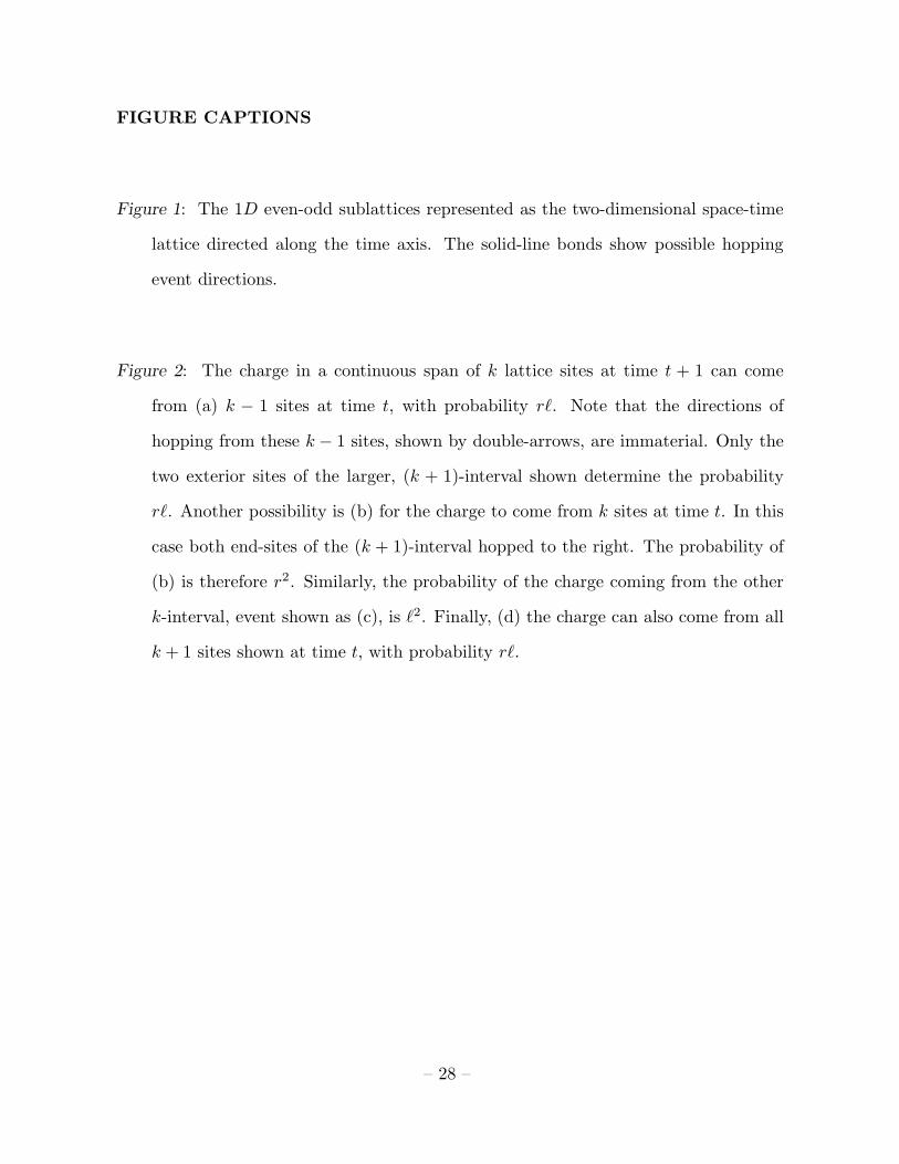
FIGURE CAPTIONS

Figure 1: The 1D even-odd sublattices represented as the two-dimensional space-time

lattice directed along the time axis. The solid-line bonds show possible hopping

event directions.

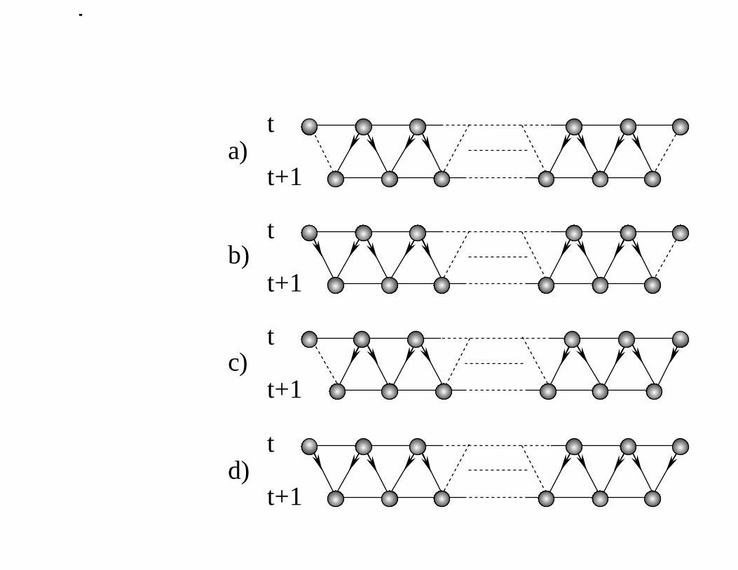
Figure 2: The charge in a continuous span of k lattice sites at time t + 1 can come

from (a) k − 1 sites at time t, with probability rℓ. Note that the directions of

hopping from these k − 1 sites, shown by double-arrows, are immaterial. Only the

two exterior sites of the larger, (k + 1)-interval shown determine the probability

rℓ. Another possibility is (b) for the charge to come from k sites at time t. In this

case both end-sites of the (k + 1)-interval hopped to the right. The probability of

(b) is therefore r2. Similarly, the probability of the charge coming from the other

k-interval, event shown as (c), is ℓ2. Finally, (d) the charge can also come from all

k + 1 sites shown at time t, with probability rℓ.

– 28 –

t

i+2 . . .i-2 i i+1i-1. . .

t

t+1a)

b)t

t+1

t

t+1d)

c)t

t+1