EDUCATION Revista Mexicana de F´ ısica E 59 (2013) 28–50 JANUARY–JUNE 2013 Exact solution of the 1D riemann problem in Newtonian and relativistic hydrodynamics F. D. Lora-Clavijo, J. P. Cruz-P´ erez, F. Siddhartha Guzm´ an, and J. A. Gonz´ alez Instituto de F´ ısica y Matem ´ aticas, Universidad Michoacana de San Nicol´ as de Hidalgo, Edificio C-3, Cd. Universitaria, 58040 Morelia, Michoac´ an, M´ exico. Received 10 August 2012; accepted 15 February 2013 Some of the most interesting scenarios that can be studied in astrophysics, contain fluids and plasma moving under the influence of strong gravitational fields. To study these problems it is required to implement numerical algorithms robust enough to deal with the equations describing such scenarios, which usually involve hydrodynamical shocks. It is traditional that the first problem a student willing to develop research in this area is to numerically solve the one dimensional Riemann problem, both Newtonian and relativistic. Even a more basic requirement is the construction of the exact solution to this problem in order to verify that the numerical implementations are correct. We describe in this paper the construction of the exact solution and a detailed procedure of its implementation. Keywords: Hydrodynamics-astrophysical applications; hydrodynamics-fluids. PACS: 95.30.Lz; 47.35.-i 1. Introduction High energy astrophysics has become one of the most impor- tant subjects in astrophysics because it involves phenomena associated to high energy radiation, modeled with sources traveling at high speeds or sources under the influence of strong gravitational fields like those due to black holes or compact stars. Current models involve a hydrodynamical de- scription of the luminous source, and therefore hydrodynam- ical equations have to be solved. In this scenario, due to the complexity of the system of equations it is required to apply numerical methods able to control the physical discontinuities arising during the evolu- tion of initial configurations, for example the evolution of the front shock in a supernova explosion, the front shock of a jet propagating in space, the edges of an accretion disk, or any shock formed during a violent process. The study of these systems involve the implementation of advanced numerical methods, being two of the most efficient and robust ones the high resolution shock capturing methods and smooth particle hydrodynamics which are representative of Eulerian and La- grangian descriptions of hydrodynamics, each one with pros and cons. It is traditional that a first step to evaluate how appropri- ate the implementation of a numerical method is, requires the comparison of numerical results with an exact solution in a simple situation. The simplest problem in hydrodynamics is the 1D Riemann problem. This is an excellent test case be- cause it has an exact solution in the Newtonian case (e.g. [1]) and also in the relativistic regime [2,3], where codes deal- ing with high Lorentz factors are expected to work properly. From our experience we have found that the existent liter- ature about the construction of the exact solution is not as explicit as it may be expected by students having their first contact with this subject. This is the reason why we present a paper that is very detailed in the construction and imple- mentation of the solution. We focus on the solution of the problem and omit some of the mathematical background that is actually very well described in the literature. The paper is organized as follows. In Sec. 2 we present the Newtonian Riemann problem and how to implement it; in Sec. 2 we present the exact solution to the relativistic case and how to implement it. Finally in Sec. 3 we present some final comments. 2. Riemann problem for the Newtonian Euler equations The Riemann problem is an initial value problem for a gas with discontinuous initial data, whose evolution is ruled by Euler’s equations. The set of Euler’s equations determine the evolution of the density of gas, its velocity field and either its pressure or total energy. A comfortable way of writing such equations involves a flux balance form as follows ∂ t u + ∂ x F(u)=0 (1) where u =(u 1 ,u 2 ,u 3 ) T =(ρ, ρv, E) T is a set of conser- vative variables and F is a flux vector, where ρ is the mass density of the gas, v its velocity and E = ρ((1/2)v 2 + ε), with ε the specific internal energy of the gas. The enthalpy of the system is given by the expression H = (1/2)v 2 + h, where h is the specific internal enthalpy given by h = ε+p/ρ, where p is the pressure of the gas. The fluxes are explicitly in terms of the primitive variables ρ, v, p and the conservative variables [1] F(u)= ρv ρv 2 + p v(E + p) = u 2 1 2 (3 - Γ) u 2 2 u1 + (Γ - 1)u 3 Γ u 2 u 1 u 3 - 1 2 (Γ - 1) u 3 2 u 2 1 .

Welcome message from author
This document is posted to help you gain knowledge. Please leave a comment to let me know what you think about it! Share it to your friends and learn new things together.
Transcript

EDUCATION Revista Mexicana de Fısica E59 (2013) 28–50 JANUARY–JUNE 2013
Exact solution of the 1D riemann problem in Newtonianand relativistic hydrodynamics
F. D. Lora-Clavijo, J. P. Cruz-Perez, F. Siddhartha Guzman, and J. A. GonzalezInstituto de Fısica y Matematicas, Universidad Michoacana de San Nicolas de Hidalgo,
Edificio C-3, Cd. Universitaria, 58040 Morelia, Michoacan, Mexico.
Received 10 August 2012; accepted 15 February 2013
Some of the most interesting scenarios that can be studied in astrophysics, contain fluids and plasma moving under the influence of stronggravitational fields. To study these problems it is required to implement numerical algorithms robust enough to deal with the equationsdescribing such scenarios, which usually involve hydrodynamical shocks. It is traditional that the first problem a student willing to developresearch in this area is to numerically solve the one dimensional Riemann problem, both Newtonian and relativistic. Even a more basicrequirement is the construction of the exact solution to this problem in order to verify that the numerical implementations are correct. Wedescribe in this paper the construction of the exact solution and a detailed procedure of its implementation.
Keywords:Hydrodynamics-astrophysical applications; hydrodynamics-fluids.
PACS: 95.30.Lz; 47.35.-i
1. Introduction
High energy astrophysics has become one of the most impor-tant subjects in astrophysics because it involves phenomenaassociated to high energy radiation, modeled with sourcestraveling at high speeds or sources under the influence ofstrong gravitational fields like those due to black holes orcompact stars. Current models involve a hydrodynamical de-scription of the luminous source, and therefore hydrodynam-ical equations have to be solved.
In this scenario, due to the complexity of the system ofequations it is required to apply numerical methods able tocontrol the physical discontinuities arising during the evolu-tion of initial configurations, for example the evolution of thefront shock in a supernova explosion, the front shock of a jetpropagating in space, the edges of an accretion disk, or anyshock formed during a violent process. The study of thesesystems involve the implementation of advanced numericalmethods, being two of the most efficient and robust ones thehigh resolution shock capturing methods and smooth particlehydrodynamics which are representative of Eulerian and La-grangian descriptions of hydrodynamics, each one with prosand cons.
It is traditional that a first step to evaluate how appropri-ate the implementation of a numerical method is, requires thecomparison of numerical results with an exact solution in asimple situation. The simplest problem in hydrodynamics isthe 1D Riemann problem. This is an excellent test case be-cause it has an exact solution in the Newtonian case (e.g.[1])and also in the relativistic regime [2,3], where codes deal-ing with high Lorentz factors are expected to work properly.From our experience we have found that the existent liter-ature about the construction of the exact solution is not asexplicit as it may be expected by students having their firstcontact with this subject. This is the reason why we presenta paper that is very detailed in the construction and imple-
mentation of the solution. We focus on the solution of theproblem and omit some of the mathematical background thatis actually very well described in the literature.
The paper is organized as follows. In Sec. 2 we presentthe Newtonian Riemann problem and how to implement it;in Sec. 2 we present the exact solution to the relativistic caseand how to implement it. Finally in Sec. 3 we present somefinal comments.
2. Riemann problem for the Newtonian Eulerequations
The Riemann problem is an initial value problem for a gaswith discontinuous initial data, whose evolution is ruled byEuler’s equations. The set of Euler’s equations determine theevolution of the density of gas, its velocity field and either itspressure or total energy. A comfortable way of writing suchequations involves a flux balance form as follows
∂tu + ∂xF(u) = 0 (1)
whereu = (u1, u2, u3)T = (ρ, ρv, E)T is a set of conser-vative variables andF is a flux vector, whereρ is the massdensity of the gas,v its velocity andE = ρ((1/2)v2 + ε),with ε the specific internal energy of the gas. The enthalpyof the system is given by the expressionH = (1/2)v2 + h,whereh is the specific internal enthalpy given byh = ε+p/ρ,wherep is the pressure of the gas. The fluxes are explicitlyin terms of the primitive variablesρ, v, p and the conservativevariables [1]
F(u)=
ρvρv2 + pv(E + p)
=
u2
12 (3− Γ)u2
2u1
+ (Γ− 1)u3
Γu2u1
u3 − 12 (Γ− 1)u3
2u2
1
.
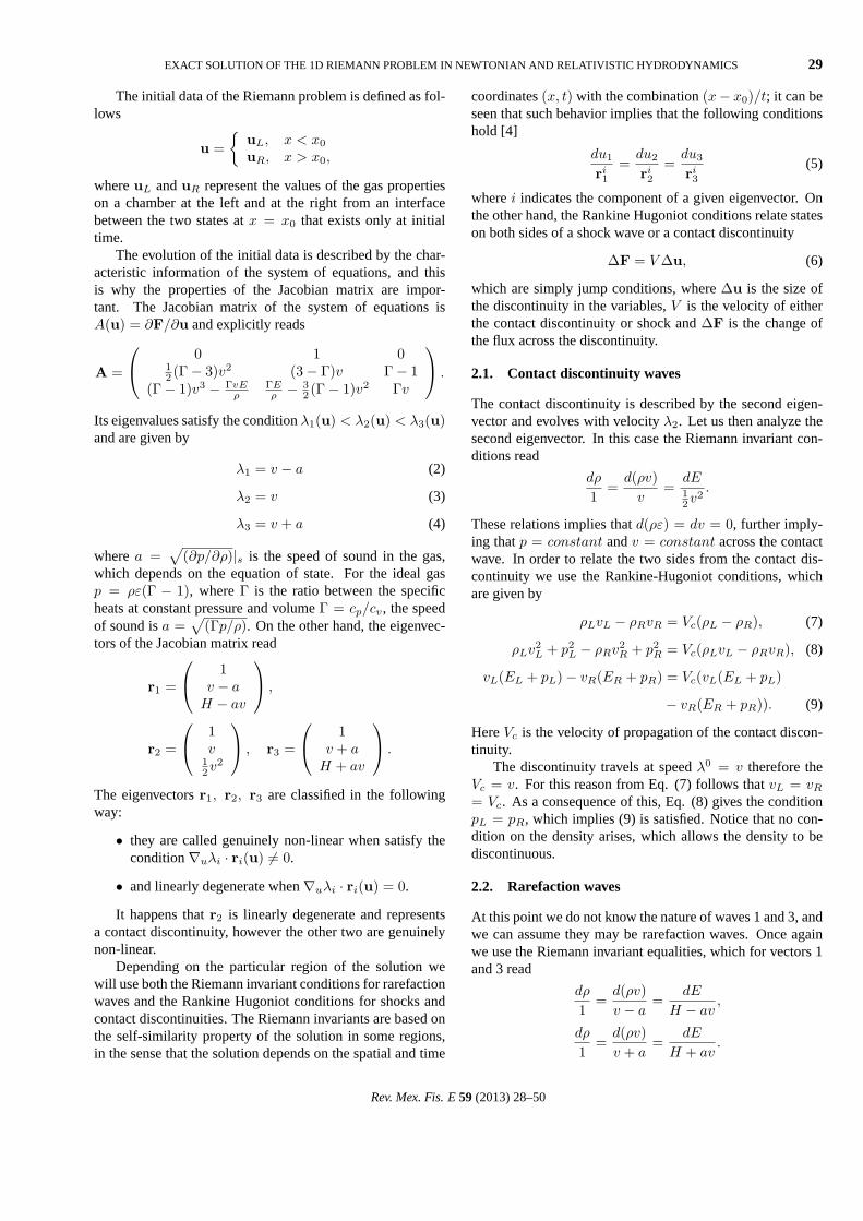
EXACT SOLUTION OF THE 1D RIEMANN PROBLEM IN NEWTONIAN AND RELATIVISTIC HYDRODYNAMICS 29
The initial data of the Riemann problem is defined as fol-lows
u ={
uL, x < x0
uR, x > x0,
whereuL anduR represent the values of the gas propertieson a chamber at the left and at the right from an interfacebetween the two states atx = x0 that exists only at initialtime.
The evolution of the initial data is described by the char-acteristic information of the system of equations, and thisis why the properties of the Jacobian matrix are impor-tant. The Jacobian matrix of the system of equations isA(u) = ∂F/∂u and explicitly reads
A =
0 1 012 (Γ− 3)v2 (3− Γ)v Γ− 1
(Γ− 1)v3 − ΓvEρ
ΓEρ − 3
2 (Γ− 1)v2 Γv
.
Its eigenvalues satisfy the conditionλ1(u) < λ2(u) < λ3(u)and are given by
λ1 = v − a (2)
λ2 = v (3)
λ3 = v + a (4)
wherea =√
(∂p/∂ρ)|s is the speed of sound in the gas,which depends on the equation of state. For the ideal gasp = ρε(Γ − 1), whereΓ is the ratio between the specificheats at constant pressure and volumeΓ = cp/cv, the speedof sound isa =
√(Γp/ρ). On the other hand, the eigenvec-
tors of the Jacobian matrix read
r1 =
1v − a
H − av
,
r2 =
1v
12v2
, r3 =
1v + a
H + av
.
The eigenvectorsr1, r2, r3 are classified in the followingway:
• they are called genuinely non-linear when satisfy thecondition∇uλi · ri(u) 6= 0.
• and linearly degenerate when∇uλi · ri(u) = 0.
It happens thatr2 is linearly degenerate and representsa contact discontinuity, however the other two are genuinelynon-linear.
Depending on the particular region of the solution wewill use both the Riemann invariant conditions for rarefactionwaves and the Rankine Hugoniot conditions for shocks andcontact discontinuities. The Riemann invariants are based onthe self-similarity property of the solution in some regions,in the sense that the solution depends on the spatial and time
coordinates(x, t) with the combination(x− x0)/t; it can beseen that such behavior implies that the following conditionshold [4]
du1
ri1
=du2
ri2
=du3
ri3
(5)
wherei indicates the component of a given eigenvector. Onthe other hand, the Rankine Hugoniot conditions relate stateson both sides of a shock wave or a contact discontinuity
∆F = V ∆u, (6)
which are simply jump conditions, where∆u is the size ofthe discontinuity in the variables,V is the velocity of eitherthe contact discontinuity or shock and∆F is the change ofthe flux across the discontinuity.
2.1. Contact discontinuity waves
The contact discontinuity is described by the second eigen-vector and evolves with velocityλ2. Let us then analyze thesecond eigenvector. In this case the Riemann invariant con-ditions read
dρ
1=
d(ρv)v
=dE12v2
.
These relations implies thatd(ρε) = dv = 0, further imply-ing thatp = constant andv = constant across the contactwave. In order to relate the two sides from the contact dis-continuity we use the Rankine-Hugoniot conditions, whichare given by
ρLvL − ρRvR = Vc(ρL − ρR), (7)
ρLv2L + p2
L − ρRv2R + p2
R = Vc(ρLvL − ρRvR), (8)
vL(EL + pL)− vR(ER + pR) = Vc(vL(EL + pL)
− vR(ER + pR)). (9)
HereVc is the velocity of propagation of the contact discon-tinuity.
The discontinuity travels at speedλ0 = v therefore theVc = v. For this reason from Eq. (7) follows thatvL = vR
= Vc. As a consequence of this, Eq. (8) gives the conditionpL = pR, which implies (9) is satisfied. Notice that no con-dition on the density arises, which allows the density to bediscontinuous.
2.2. Rarefaction waves
At this point we do not know the nature of waves 1 and 3, andwe can assume they may be rarefaction waves. Once againwe use the Riemann invariant equalities, which for vectors 1and 3 read
dρ
1=
d(ρv)v − a
=dE
H − av,
dρ
1=
d(ρv)v + a
=dE
H + av.
Rev. Mex. Fis. E59 (2013) 28–50

30 F. D. LORA-CLAVIJO, J. P. CRUZ-PEREZ, F. SIDDHARTHA GUZMAN, AND J. A. GONZALEZ
Manipulation of these equalities results in the followingequations
dρ
dv= −ρ
afor λ1, (10)
dρ
dv=
ρ
afor λ3, (11)
dε
dρ=
p
ρ2for both λ1 and λ3. (12)
The next step is to integrate these equations assuming anequation of state, in our case the ideal gas. From (12) weobtain
p = KρΓ (13)
whereK is a constant. A rarefaction process is isentropic(unlike a shock), and therefore the states at the left and at theright from the wave obey (13) with the same constantK.
Using this expression forp in the speed of sound we havea =
√KΓρΓ−1 =
√Γp/ρ, which substituted into (10,11)
results in
v = ±∫ √
KΓρΓ−3dρ + k = ± 2a
Γ− 1+ k, (14)
where+ stands for the wave moving to the right (the case ofλ3 andr3 corresponding to a rarefaction wave) and− whenmoving to the left (the case ofλ1 andr1 corresponding toa rarefaction wave), wherek is an integration constant andtherefore the velocity is constant as well. This property al-lows us to set relations between the velocity of the gas onthe state at the left and at the right from the rarefaction wave,explicitly there are two possible cases:
i) When the wave is moving to the left, condition (14)implies that
vL +2aL
Γ− 1= vR +
2aR
Γ− 1. (15)
ii) When the wave is moving to the right, condition (14)implies
vL − 2aL
Γ− 1= vR − 2aR
Γ− 1(16)
When the wave is moving to the left, we assume informa-tion from the left state is available and we look for expressionof the variables on the state to the right from the wave. For thevelocity of the fluid at the right state we then have from (15)
vR = vL − 2Γ− 1
[aR − aL], (17)
now considering that the speed of sound on both sides obeysa =
√KΓρΓ−1 =
√Γp/ρ (see (13))
aR = aL
(pR
pL
)Γ−12Γ
, (18)
a useful expression forvR arises
vR = vL − 2aL
Γ− 1
[(pR
pL
)Γ−12Γ
− 1
]. (19)
The only unknown quantity ispR.On the other hand, when the wave is moving to the right
we assume we know the information at the state at the rightfrom the wave, then we search for expressions of the vari-ables on the state at the left. For the velocity we find accord-ing to (16)
vL = vR − 2Γ− 1
[aR − aL], (20)
and the speed of sound on both sides obeys
aL = aR
(pL
pR
)Γ−12Γ
, (21)
which finally implies
vL = vR − 2aR
Γ− 1
[1−
(pL
pR
)Γ−12Γ
]. (22)
The only unknown quantity in this case ispL.The rarefaction zone has a finite size, bounded by two
curves, the tail and the head. The head of the wave is the lineof the front of the wave and the tail is the boundary left be-hind the wave. The region in the middle is called the fan ofthe rarefaction wave.
The velocity of all the particles between the head and thetail obeys the following expression
x− x0
t= v ± a, (23)
where + is used when the wave is propagating to the rightand the - when it is moving to the left. Then, when thewave is moving to the left, using this expression we haveaR = vR − (x− x0)/t, which substituted into (19) providesthe following expression for the velocity of the gas on thestate at the right from the wave is
vR =2
Γ + 1
[aL +
12(Γ− 1)vL +
x− x0
t
]. (24)
Then it is possible to calculate the pressure and densityas well. Substituting (24) into (15) and (18) we obtain anexpression for the pressure also at the state to the right
pR=pL
[2
Γ + 1+
Γ− 1aL(Γ + 1)
(vL−x− x0
t
)] 2ΓΓ−1
. (25)
Now, using this into (13) implies the expression for the den-sity
ρR=ρL
[2
Γ + 1+
Γ− 1aL(Γ + 1)
(vL−x− x0
t
)] 2Γ−1
. (26)
Rev. Mex. Fis. E59 (2013) 28–50
EXACT SOLUTION OF THE 1D RIEMANN PROBLEM IN NEWTONIAN AND RELATIVISTIC HYDRODYNAMICS 31
Then finally we have expressions for the velocity, pressureand density on the state at the right when the wave is movingto the left.Similarly when the wave is moving to the right we havefrom (23) thataL = vL + (x − x0)/t, which substitutedinto (22) implies the following for the velocity on the state atthe left from the wave
vL =2
Γ + 1
[−aR +
12(Γ− 1)vR +
x− x0
t
]. (27)
In order to obtain the expressions for the pressure and thedensity, we substitute this last expressions into (16) in orderto relate the speeds of sound, and then using (21) we finallyobtain the expression for the pressure at the left
pL=pR
[2
Γ + 1− Γ− 1
aR(Γ + 1)
(vR−x− x0
t
)] 2ΓΓ−1
. (28)
Finally using the Eq. (13) we obtain the density
ρL=ρR
[2
Γ+1− Γ−1
aR(Γ+1)
(vR−x−x0
t
)] 2Γ−1
. (29)
In this way we have relations between the variables on to thestate at the left and at the right from a rarefaction wave. Theserelations will be useful when solving the Riemann problem.
2.3. Shock waves
Similar to the previous case, the shock can move either tothe right (if λ3 andr3 correspond to a shock wave) or to theleft (if λ1 andr1 correspond to a shock wave), and for eachof the two cases there is known and unknown information.When a shock is moving to the right one is expected to haveinformation of the state at the right from the shock and con-versely, when the shock is moving to the left one accountswith information of the state at the left.
Shocks require the use of Rankine Hugoniot condi-tions (6). We express these conditions in terms of the primi-tive variables as follows
ρLvL − ρRvR = S(ρL − ρR),
ρLv2L + pL − ρRv2
R − pR = S(ρLvL − ρRvR),
vL(EL + pL)− vR(ER + pR) = S(EL − ER),
whereS is the speed of the wave, which may take the valuesv − a or v + a depending on whether the wave moves to theleft or to the right respectively. Manipulating these equationsone gets
ρLvL = ρRvR, (30)
ρLv2L + pL = ρRv2
R + pR, (31)
vL(EL + pL) = vR(ER + pR), (32)
where vL = vL − S, vR = vR − S are velocities in therest frame of the shock andEL = ρL
((1/2)v2
L + εL
)and
ER = ρR
((1/2)v2
R + εR
). These expressions correspond to
the Rankine Hugoniot jump conditions measured by an ob-server located in the rest frame of the shock wave.
From Eq. (30), we introduce the mass flux definition
j = ρLvL = ρRvR. (33)
Then, from Eq. (31) and the mass flux definition before men-tioned, we can get an expression forj, which is given by
j = −pR − pL
vR − vL= −pR − pL
vR − vL, (34)
which is a consequence ofj being invariant under Galileantransformations. Considering the shock is moving to the left,we would be interested in constructing the variables on thestate at the right from the shock and we can start with thevelocity, which can be written as
vR = vL − pR − pL
j. (35)
Now, in order to express the velocity in terms of the pressureand the variables of the state at the left from the shock, wecan rewrite (33) as follows
vR − S =j
ρR, vL − S =
j
ρL. (36)
Thus, substituting this into (34) we obtain
j2 = − pR − pL1
ρR− 1
ρL
. (37)
On the other hand, using Eq. (32) and the expression for thespecific internal enthalpyh we can easily get the followingexpression for the difference of internal specific enthalpies
hR − hL =12
[v2
L − v2R
], (38)
wherehL = εL + pL/ρL andhR = εR + pR/ρR. Now,from Eqs. (30) and (31) we give expressions for the veloci-tites measured by the observer located in the rest frame of theshock wave
v2R =
ρL
ρR
pL − pR
ρL − ρR,
v2L =
ρR
ρL
pL − pR
ρL − ρR.
With the substitution of these last equations into (38) andconsidering the definitions for the specific internal enthalpymentioned above, we obtain
εR − εL =12
(pL + pR)(ρR − ρL)ρLρR
.
Assuming the gas obeys an ideal equation of state we get anexpression for the density as follows
ρR
ρL=
pL(Γ− 1) + pR(Γ + 1)pR(Γ− 1) + pL(Γ + 1)
. (39)
Rev. Mex. Fis. E59 (2013) 28–50
32 F. D. LORA-CLAVIJO, J. P. CRUZ-PEREZ, F. SIDDHARTHA GUZMAN, AND J. A. GONZALEZ
Notice that this expression relates the density among thetwo sides from the shock. Now, substituting this expressioninto (37) we obtain
j2 =pR + BL
AL,
AL =2
(Γ + 1)ρL, BL =
Γ− 1Γ + 1
pL. (40)
Thus, the expression for the velocity (35) can be written asfollows
vR = vL − (pR − pL)
√AL
pR + BL. (41)
From expression (36) and using (40) we express the shockvelocity as follows
S = vL −√
pR(Γ + 1) + pL(Γ− 1)2ρL
.
Finally, using the sound speed expressionaL=√
pLΓ/ρL weobtain the final expression for the shock velocity
S = vL − aL
√(Γ + 1)pR
2pLΓ+
Γ− 12Γ
. (42)
Analogously, when the shock moves to the right, it is pos-sible to construct the expressions for the variables for the stateat the left from the shock
vL = vR + (pL − pR)
√AR
pL + BR, (43)
ρL = ρRpR(Γ− 1) + pL(Γ + 1)pL(Γ− 1) + pR(Γ + 1)
, (44)
S = vR + aR
√(Γ + 1)pL
2pRΓ+
Γ− 12Γ
. (45)
and we let this as an exercise to the reader.
2.4. Classical Riemann Problem
The Riemann problem is physically a tube filled with gaswhich is divided into two chambers separated by a remov-able membrane atx = x0. At the initial time the membraneis removed and the gas begins to flow. Once the membrane isremoved, the discontinuity decays into two elementary, non-linear waves that move in opposite directions.
Depending on the values of the thermodynamical vari-ables in each chamber, four cases can occur. Considering thefluid is described on a one-dimensional spatial domain, rar-efaction and shock waves can evolve toward the left or rightfrom the location of the membrane.
In general the solution in all the cases can be studied insix following regions:
Region 1: initial left state that has not been yet influ-enced by rarefaction or shock waves
Region 2: wave traveling to the left (may be rarefactionor shock)
Region 3: region between the wave moving to the leftand the contact discontinuity, called region star-left
Contact discontinuity
Region 4: region between the contact discontinuity andthe wave moving to the right, called region star-right
Region 5: wave traveling to the right (may be rarefac-tion or shock)
Region 6: initial right state that has not been yet influ-enced by rarefaction or shock waves
Regions 2 and 5 are special. If the wave propagating in suchregions is a rarefaction wave the region involves a head-fan-tail structure, whereas if it is a shock the region becomes onlya discontinuity. Counting from left to right on the spatial do-main, the results can be reduced to the following four possiblecombinations of waves:
1) rarefaction-shock
2) shock-rarefaction
3) rarefaction-rarefaction
4) shock-shock
with a contact discontinuity between the two waves in allcases. It is worth noticing that these combinations can occurunder a wide variety of possible combinations of the initialvalues of the thermodynamical variables. In this paper we il-lustrate each of these scenarios using particular sets of initialconditions.
2.4.1. Case 1: Rarefaction-Shock
This case corresponds to the typical case used to test numer-ical codes, a test called the Sod’s shock tube problem [5].A traditional set of initial values that produces this scenariocorresponds to a gas with higher density and pressure in theleft chamber than in the right chamber, and the velocity is setinitially to zero in both.
A rarefaction wave travels into the high density region(moves to the left), whereas a shock moves into the low den-sity region (moves to the right).
Summarizing, the problem then involves five regionsonly. Regions 1 correspond to the initial state to the left thathas not been influenced by the evolution of the system. Re-gion 2 corresponds to a rarefaction wave containing the head-fan-tail structure, region 3 and 4 are the left and right statesseparated by the contact discontinuity. Region 5 reduces tothe shock. Finally region 6 is the initial state at the right
Rev. Mex. Fis. E59 (2013) 28–50

EXACT SOLUTION OF THE 1D RIEMANN PROBLEM IN NEWTONIAN AND RELATIVISTIC HYDRODYNAMICS 33
chamber that has not been influenced by the evolution of thesystem.
The goal is to determine the state in all the regions usingthe relations between the thermodynamical quantities con-structed before.
The starting point to construct the solution happens at thecontact discontinuity, where the velocity and pressure obeythe conditionsp3 = p4 = p∗ andv3 = v4 = v∗.
Region 3 plays the role of the state at the right from therarefaction wave and region 1 the state at the left. Then wecan use (19) to obtain an expression forv3
v3 = v1 − 2a1
Γ− 1
[(p3
p1
)Γ−12Γ
− 1
]. (46)
On the other hand, region 4 plays the role of a state at the leftfrom the shock wave and region 6 the role of the state at theright. Then we use (43) to calculatev4:
v4 = v6 + (p4 − p6)
√A6
p4 + B6. (47)
whereA6 = 2/ρ6/(Γ + 1) andB6 = p6(Γ − 1)/(Γ + 1).Given thatv3 = v4 = v∗, equating both expressions oneobtains a trascendental equation forp∗:
(p∗ − p6)
√A6
p∗ + B6
+2a1
Γ− 1
[(p∗
p1
)Γ−12Γ
− 1
]+ v6 − v1 = 0. (48)
Unfortunately as far as we can tell, no exact solution is knownfor p∗, and then we proced to construct its solution numeri-cally. Once this equation is solved,p3 andp4 are automat-ically known, andv3 and v4 can be calculated using (46)and (47) respectively.
Then, it is possible to calculateρ3 using (13) at both sidesof the rarefaction zone, givenC is the same on both sides be-cause it is an isentropic process:
ρ3 = ρ1
(p3
p1
)1/Γ
(49)
where nowp1, ρ1 andp3 are known. On the other hand onecan also calculateρ4 using (44)
ρ4 = ρ6
(p6(Γ− 1) + p4(Γ + 1)p4(Γ− 1) + p6(Γ + 1)
)(50)
also in terms of known information. With this information itis already possible to construct the solution in the whole do-main. We explain how to do it region by region. A scheme ofhow the regions are distributed is shown in Fig. 1.
1. Region 1 is defined by the conditionx − x0 < tVhead,whereVheadis the velocity of the head of the rarefactionwave given by the characteristic value of the Jacobian
matrix evaluated at the location next to the head fromthe left side, that is, considering (2)Vh = v1−a1. Thesolution there is simply
pexact = p1,
vexact = v1,
ρexact = ρ1.
2. Region 2 is defined by the conditiontVhead < x −x0 < tVtail, whereVtail is the same characteristic valueagain, but this time evaluated at the tail curve, that isVtail = v3 − a3. This is the fan region for a rarefactionwave moving to the left, for which we simply use ex-pressions (24,25,26) that need only information fromregion 1 and obtain
ρexact=ρ1
[2
Γ+1+
Γ−1a1(Γ+1)
(v1−x− x0
t
)] 2Γ−1
,
pexact=p1
[2
Γ+1+
Γ−1a1(Γ+1)
(v1−x− x0
t
)] 2ΓΓ−1
,
vexact=2
Γ+1
[a1+
12(Γ−1)v1+
x−x0
t
]. (51)
3. Region 3 is defined by the conditiontVtail < x− x0 <tVcontact, whereVcontact is the velocity of the contactdiscontinuity, which is the second eigenvalue (3) ofthe Jacobian matrix evaluated at this region, that isVcontact= v3 = v4. The solution there finally reads
pexact = p3,
vexact = v3,
ρexact = ρ3.
4. Region 4 is defined by the conditiontVcontact < x −x0 < tVshock, where according to (45), the velocity ofa shock moving to the right separating regions 4 and 6is
Vshock = v6 + a6
√(Γ + 1)p4
2Γp6+
Γ− 12Γ
,
wherea6 =√
p6Γ/ρ6. Then the solution in this regionis
pexact = p4,
vexact = v4,
ρexact = ρ4.
as calculated
5. There is no region 5.
Rev. Mex. Fis. E59 (2013) 28–50

34 F. D. LORA-CLAVIJO, J. P. CRUZ-PEREZ, F. SIDDHARTHA GUZMAN, AND J. A. GONZALEZ
6. Region 6 is defined bytVshock < x− x0. In this regionthe solution is simply
pexact= p6,
vexact= v6,
ρexact= ρ6.
An example of how the solution looks like is shown inFig. 2 for initial data in Table I.
TABLE I. Table with the initial data for the four different cases. Wechoose the spatial domain to bex ∈ [0, 1] and the location of themembrane atx0 = 0.5. In all cases we useΓ = 1.4.
Case pL pR vL vR ρL ρR
Rarefaction-Shock 1.0 0.1 0.0 0.0 1.0 0.125
Shock-Rarefaction 0.1 1.0 0.0 0.0 0.125 1.0
Rarefaction-Rarefaction 0.4 0.4 -1.0 1.0 1.0 1.0
Shock-Shock 0.4 0.4 1.0 -1.0 1.0 1.0
FIGURE 1. Description of the relevant regions for the Rarefaction-Shock case.
FIGURE 2. Exact solution for the Rarefaction-Shock case at timet = 0.25 for the parameters in Table I.
2.4.2. Case 2: Shock-Rarefaction
This case is identical to the previous one, except that wechoose the initial pressure and density are higher on the rightchamber. After initial time, the wave traveling to the left isa shock, while the one moving to the right is a rarefactionwave. This implies that region 2 plays the role of region 5 inthe previous case and region 5 has the tail-fan-head structureof a rarefaction wave.
Starting from the contact discontinuity, the conditionsv3 = v4 = v∗ and p3 = p4 = p∗ hold. The conditionson a shock wave moving to the left imply according to (41)that the velocity of the state at the right is
v3 = v1 − (p3 − p1)
√A1
p3 + B1, (52)
and information from the rarefaction wave interface can beobtained from (27) forv4 as the velocity on the state at theleft from a rarefaction wave moving to the right
v4 = v6 − 2a6
Γ− 1
[1−
(p4
p6
)Γ−12Γ
]. (53)
Equating these two expression one obtains a trascendentalequation forp∗:
− (p∗ − p1)
√A1
p∗ + B1
+2a6
Γ− 1
[1−
(p∗
p6
)Γ−12Γ
]+ v1 − v6 = 0 (54)
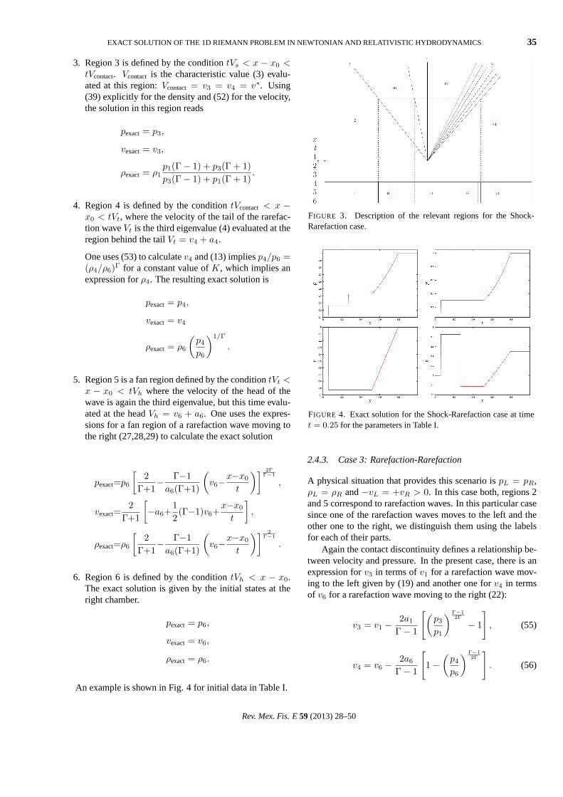
that one solves numerically forp∗. This information pro-vides the necessary information to construct the solution inthe whole domain as described below. The different regionsare illustrated in Fig. 3 and the exact solution region by re-gion is as follows.
1. Region 1 is defined byx− x0 < tVshock, where the ve-locity of the shock is given by (42) because the shockis traveling to the left:
Vs = v1 − a1
√(Γ + 1)p3
2p1Γ+
Γ− 12Γ
,
and the exact solution here reads
pexact= p1,
vexact= v1,
ρexact= ρ1.
2. There is no region 2.
Rev. Mex. Fis. E59 (2013) 28–50
EXACT SOLUTION OF THE 1D RIEMANN PROBLEM IN NEWTONIAN AND RELATIVISTIC HYDRODYNAMICS 35
3. Region 3 is defined by the conditiontVs < x − x0 <tVcontact. Vcontact is the characteristic value (3) evalu-ated at this region:Vcontact = v3 = v4 = v∗. Using(39) explicitly for the density and (52) for the velocity,the solution in this region reads
pexact = p3,
vexact = v3,
ρexact = ρ1p1(Γ− 1) + p3(Γ + 1)p3(Γ− 1) + p1(Γ + 1)
.
4. Region 4 is defined by the conditiontVcontact < x −x0 < tVt, where the velocity of the tail of the rarefac-tion waveVt is the third eigenvalue (4) evaluated at theregion behind the tailVt = v4 + a4.
One uses (53) to calculatev4 and (13) impliesp4/p6 =(ρ4/ρ6)Γ for a constant value ofK, which implies anexpression forρ4. The resulting exact solution is
pexact= p4,
vexact= v4
ρexact= ρ6
(p4
p6
)1/Γ
.
5. Region 5 is a fan region defined by the conditiontVt <x − x0 < tVh where the velocity of the head of thewave is again the third eigenvalue, but this time evalu-ated at the headVh = v6 + a6. One uses the expres-sions for a fan region of a rarefaction wave moving tothe right (27,28,29) to calculate the exact solution
pexact=p6
[2
Γ+1− Γ−1
a6(Γ+1)
(v6−x−x0
t
)] 2ΓΓ−1
,
vexact=2
Γ+1
[−a6+
12(Γ−1)v6+
x−x0
t
],
ρexact=ρ6
[2
Γ+1− Γ−1
a6(Γ+1)
(v6−x−x0
t
)] 2Γ−1
.
6. Region 6 is defined by the conditiontVh < x − x0.The exact solution is given by the initial states at theright chamber.
pexact = p6,
vexact = v6,
ρexact = ρ6.
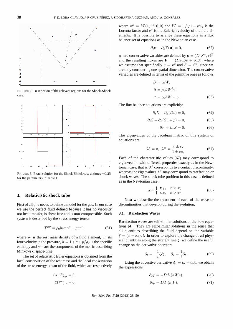
An example is shown in Fig. 4 for initial data in Table I.
FIGURE 3. Description of the relevant regions for the Shock-Rarefaction case.
FIGURE 4. Exact solution for the Shock-Rarefaction case at timet = 0.25 for the parameters in Table I.
2.4.3. Case 3: Rarefaction-Rarefaction
A physical situation that provides this scenario ispL = pR,ρL = ρR and−vL = +vR > 0. In this case both, regions 2and 5 correspond to rarefaction waves. In this particular casesince one of the rarefaction waves moves to the left and theother one to the right, we distinguish them using the labelsfor each of their parts.
Again the contact discontinuity defines a relationship be-tween velocity and pressure. In the present case, there is anexpression forv3 in terms ofv1 for a rarefaction wave mov-ing to the left given by (19) and another one forv4 in termsof v6 for a rarefaction wave moving to the right (22):
v3 = v1 − 2a1
Γ− 1
[(p3
p1
)Γ−12Γ
− 1
], (55)
v4 = v6 − 2a6
Γ− 1
[1−
(p4
p6
)Γ−12Γ
]. (56)
Rev. Mex. Fis. E59 (2013) 28–50

36 F. D. LORA-CLAVIJO, J. P. CRUZ-PEREZ, F. SIDDHARTHA GUZMAN, AND J. A. GONZALEZ
The conditionv3 = v4 = v∗ at the contact discontinuity im-plies a trascendental equation forp∗ = p3 = p4:
2a6
Γ− 1
[1−
(p∗
p6
)Γ−12Γ
]
− 2a1
Γ− 1
[(p∗
p1
)Γ−12Γ
− 1
]+ v1 − v6 = 0 (57)
Again, oncep∗ is calculated numerically, the solution inall the regions of the domain can be calculated as follows.The first implication is thatp3 = p4 = p∗, and thusv3 andv4
can be calculated using (55) and (56). The different regionsare illustrated in Fig. 5.
1. Region 1 is defined by the conditionx − x0 < tVh,2,whereVh,2 is the velocity of the head of the wave mov-ing to the left, and is obtained from the characteristicvalue of such rarefaction wave evaluated at the left in-terface, that isVh,2 = v1 − a1. In this region the gashas not affected the initial state on the left, then thesolution is
pexact= p1,
vexact= v1,
ρexact= ρ1.
2. Region 2 is a fan region defined by the conditiontVh,2 < x − x0 < tVt,2, where the velocity of thetail Vt,2 is that of the state left behind by the wave, thatis Vt,2 = v3 − a3.
The exact solution is that of a fan region of a rarefac-tion wave moving to the left (24-26)
pexact=p1
[2
Γ+1+
Γ−1a1(Γ+1)
(v1−x− x0
t
)] 2ΓΓ−1
,
vexact=2
Γ+1
[a1+
12(Γ− 1)v1+
x− x0
t
],
ρexact=ρ1
[2
Γ + 1+
Γ− 1a1(Γ + 1)
(v1−x− x0
t
)] 2Γ−1
.
3. Region 3 is defined by the conditiontVt,2 < x− x0 <tVcontact. The velocity of the contact discontinuity isVcontact = v3 = v4 = v∗ according to the eigen-value (3). In this regionp3 = p∗ and v3 = v∗ arealready known fromp∗. Finally, the density is obtainedfrom (13) for an isentropic process like the rarefactionwave for a constantC on both sides of such wave asfound in the previous two cases. Thus the solution is
pexact = p3,
vexact = v3.
ρexact = ρ1
(p3
p1
)1/Γ
,
4. Region 4 is defined by the conditiontVcontact < x −x0 < tVt,5, where the velocity of the tail of the wavemoving to the rightVt,5 is given by the eigenvalue (4)evaluated at the state left behind the rarefaction wavemoving to the right, that isVt,5 = v4 +a4, where againwe point out thatv4 = v∗ and p4 = p∗ are knownoncep∗ is calculated. The solution is obtained in thesame way as for the previous region, but now the waverelates states in regions 4 and 6:
pexact= p4,
vexact= v4.
ρexact= ρ6
(p4
p6
)1/Γ
,
5. Region 5 is defined by the conditiontVt,5 < x− x0 <Vh,5, where the velocity of the head of the wave mov-ing to the right isVh,5 = v6+a6, and the solution is ob-tained using the values of the state variables for the fanof a rarefaction wave moving to the right (27,28,29):
pexact=p6
[2
Γ + 1− Γ− 1
a6(Γ + 1)
(v6−x− x0
t
)] 2ΓΓ−1
,
vexact=2
Γ + 1
[−a6+
12(Γ− 1)v6+
x− x0
t
],
ρexact=ρ6
[2
Γ + 1− Γ− 1
a6(Γ + 1)
(v6 − x− x0
t
)] 2Γ−1
.
6. Finally, region 6 is defined by the conditionVh,5 <x−x0. The exact solution is given by the initial valuesat the chamber on the right because in this region thegas has not been affected yet by the dynamics of thegas:
pexact = p6,
vexact = v6,
FIGURE 5. Description of the relevant regions for the Rarefaction-Rarefaction case.
Rev. Mex. Fis. E59 (2013) 28–50

EXACT SOLUTION OF THE 1D RIEMANN PROBLEM IN NEWTONIAN AND RELATIVISTIC HYDRODYNAMICS 37
FIGURE 6. Exact solution for the Rarefaction-Rarefaction case attime t = 0.25 for the parameters in Table I.
ρexact = ρ6.
An example is shown in Fig. 6 for initial data in Table I.
2.4.4. Case 4: Shock-Shock
A physical situation that provides this scenario correspondsto two streams colliding with opposite directions. We choosein this casepL = pR, ρL = ρR and−vL = +vR < 0. In thiscase regions 2 and 5 are shock waves.
Again the contact discontinuity defines a relationship be-tween velocity and pressure. In the present case there is anexpression forv3 in terms ofv1 for a shock-wave moving tothe left given by (41) and another one forv4 in terms ofv6
for a shock-wave moving to the right (43):
v3 = v1 − (p3 − p1)
√A1
p3 + B1, (58)
v4 = v6 + (p4 − p6)
√A6
p4 + B6. (59)
The conditionv3 = v4 = v∗ at the contact discontinuity im-plies a trascendental equation forp∗ = p3 = p4:
− (p∗ − p1)
√A1
p∗ + B1
− (p∗ − p6)
√A6
p∗ + B6+ v1 − v6 = 0. (60)
Again, oncep∗ is calculated numerically, the solution inall the regions of the domain can be calculated as follows.Immediately one has thatp3 = p4 = p∗ andv3 andv4 can becalculated using (58) and (59).
In this particular case regions 2 and 5 reduce to lines. Thesolution in each region reads as follows and the regions areillustrated in Fig. 7.
1. Region 1 is defined by the conditionx − x0 < tVs,2,where the velocity of the shock moving to the leftVs,2
is given by (42) and reads
Vs,2 = v1 − a1
√(Γ + 1)p3
2p1Γ+
Γ− 12Γ
.
The solution there is that of the initial values of thevariables on the left chamber:
pexact = p1,
vexact = v1,
ρexact = ρ1.
2. There is no region 2.
3. Region 3 is defined by the conditiontVs,2 < x − x0
< tVcontact, whereVcontact = v3 = v4 = v∗. Once (54)is solved one can calculate all the required informa-tion. Using (58) forv3 and (39) forρ3 the solution inthis region reads
pexact= p3,
vexact= v3
ρexact= ρ1p1(Γ− 1) + p3(Γ + 1)p3(Γ− 1) + p1(Γ + 1)
.
4. Region 4 is defined bytVcontact < x − x0 < tVs,5,where the velocity of the shock moving to the right isgiven by (45) and reads
Vs,5 = v6 + a6
√(Γ + 1)p4
2p6Γ+
Γ− 12Γ
.
Finally, using (59) forv4 and (44) forρ4 the solutionin this region reads
pexact= p4,
vexact= v4,
ρexact= ρ6p6(Γ− 1) + p4(Γ + 1)p4(Γ− 1) + p6(Γ + 1)
.
5. There is no region 5.
6. Finally region 6 is defined by the conditionVs,5 <x−x0. The exact solution is given by the initial valuesat the chamber on the right:
pexact = p6,
vexact = v6,
ρexact = ρ6.
An example is shown in Fig. 8.
Rev. Mex. Fis. E59 (2013) 28–50
38 F. D. LORA-CLAVIJO, J. P. CRUZ-PEREZ, F. SIDDHARTHA GUZMAN, AND J. A. GONZALEZ
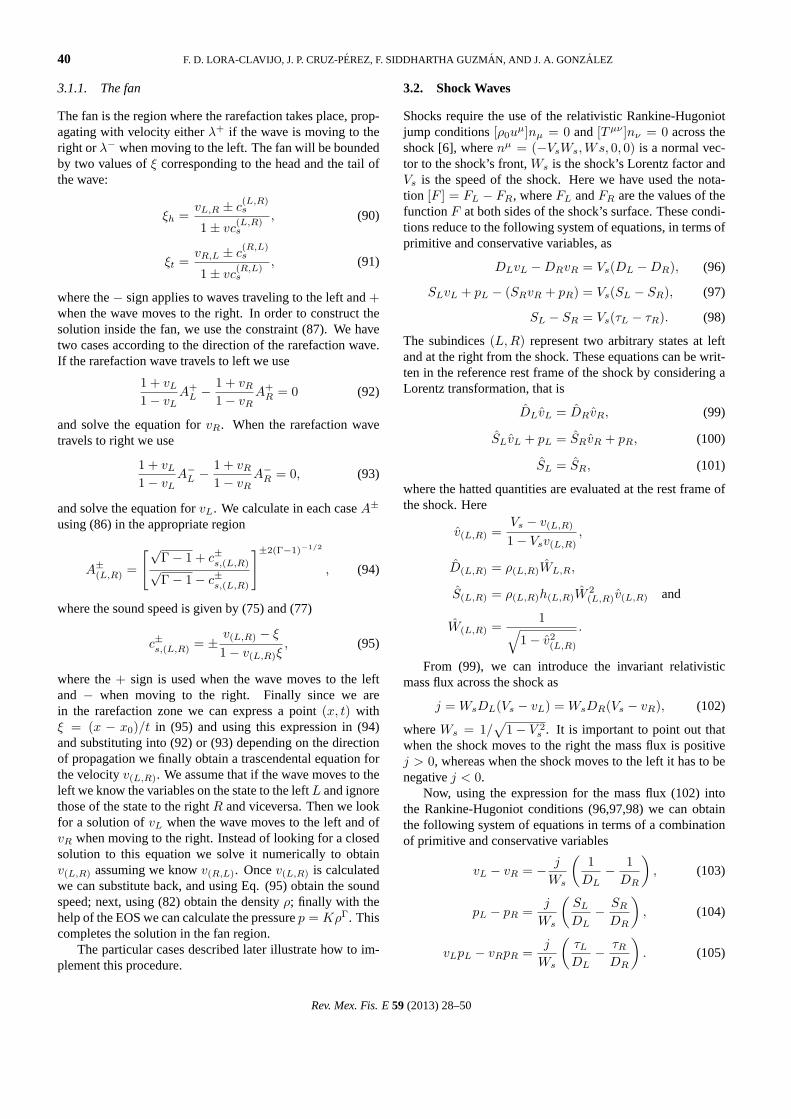
FIGURE 7. Description of the relevant regions for the Shock-Shockcase.
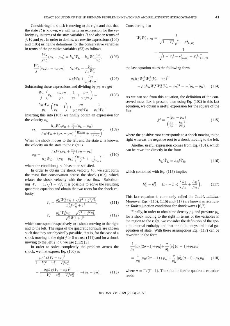
FIGURE 8. Exact solution for the Shock-Shock case at timet=0.25
for the parameters in Table I.
3. Relativistic shock tube
First of all one needs to define a model for the gas. In our casewe use the perfect fluid defined because it has no viscositynor heat transfer, is shear free and is non-compressible. Suchsystem is described by the stress energy tensor
Tµν = ρ0huµuν + pηµν , (61)
whereρ0 is the rest mass density of a fluid element,uµ itsfour velocity,p the pressure,h = 1 + ε + p/ρ0 is the specificenthalpy andηµν are the components of the metric describingMinkowski space-time.
The set of relativistic Euler equations is obtained from thelocal conservation of the rest mass and the local conservationof the stress energy tensor of the fluid, which are respectively
(ρ0uµ),µ = 0,
(Tµν),ν = 0,
whereuµ = W (1, vx, 0, 0) andW = 1/√
1− vivi is theLorentz factor andvx is the Eulerian velocity of the fluid el-ements. It is possible to arrange these equations as a fluxbalance set of equations as in the Newtonian case
∂tu + ∂xF(u) = 0, (62)
where conservative variables are defined byu = (D, Sx, τ)T
and the resulting fluxes areF = (Dv, Sv + p, S), wherewe assume that specificallyv = vx andS = Sx, since weare only considering one spatial dimension. The conservativevariables are defined in terms of the primitive ones as follows
D = ρ0W,
S = ρ0hW 2v,
τ = ρ0hW − p. (63)
The flux balance equations are explicitly:
∂tD + ∂x(Dv) = 0, (64)
∂tS + ∂x(Sv + p) = 0, (65)
∂tτ + ∂xS = 0. (66)
The eigenvalues of the Jacobian matrix of this system ofequations are
λo = v, λ± =v ± cs
1± vcs. (67)
Each of the characteristic values (67) may correspond toeigenvectors with different properties exactly as in the New-tonian case, that is,λ0 corresponds to a contact discontinuity,whereas the eigenvaluesλ± may correspond to rarefaction orshock waves. The shock tube problem in this case is definedas in the Newtonian case:
u ={
uL, x < x0
uR, x > x0.(68)
Next we describe the treatment of each of the wave ordiscontinuities that develop during the evolution.
3.1. Rarefaction Waves
Rarefaction waves are self-similar solutions of the flow equa-tions [4]. They are self-similar solutions in the sense thatall quantities describing the fluid depend on the variableξ = (x − x0)/t. In order to explore the change of all phys-ical quantities along the straight lineξ, we define the usefulchange on the derivative operators
∂t = −1tξ∂ξ, ∂x =
1t∂ξ. (69)
Using the advective derivativeda = ∂t + v∂x, we obtainthe expressions
∂xp = −Dda(hWv), (70)
∂tp = Dda(hW ), (71)
Rev. Mex. Fis. E59 (2013) 28–50

EXACT SOLUTION OF THE 1D RIEMANN PROBLEM IN NEWTONIAN AND RELATIVISTIC HYDRODYNAMICS 39
where we have used the rest mass conservation law to sim-plify the expressions. From (69) we obtain for the advectivederivativeda = (1/t)(ξ − v)d/dξ, for which we will used := d/dξ from now on. With this in mind we obtain from(70,71) the differential equation
(v − ξ)ρhW 2dv + (1− ξv)dp = 0. (72)
On the other hand, the change of variable in (64) fromt, x to ξ implies
(v − ξ)dρ + ρW 2(1− vξ)dv = 0. (73)
and from Eqs. (72) and (73) we obtain a relation between thedensity and pressure
dp = h
[v − ξ
1− vξ
]2
dρ. (74)
Since the process alongξ is isentropic [6] the sound speed is
c2s =
1h
∂p
∂ρ
∣∣∣∣s
,
which combined with the previous expression implies thespeed of sound
cs(v, ξ) =∣∣∣∣
v − ξ
1− vξ
∣∣∣∣ . (75)
Besides, we can find a useful expression for an isentropic pro-cess usingp = KρΓ (we are using a politropic equation ofstate).
cs =
√Γp
ρh. (76)
From system (67) we obtain the speed of sound in terms ofthe eigenvalues of the Jacobian matrix
cs ={ −(v − λ+)/(1− vλ+) if ξ = λ+,
(v − λ−)/(1− vλ−) if ξ = λ−.(77)
Comparing with (75) we find thatcs(v, λ+) is the speedof sound for a rarefaction wave traveling to the right andcs(v, λ−) for a wave traveling to the left.
According to this equation we get from (73) that
W 2dv ± cs
ρdρ = 0. (78)
Here the+ sign refers to the wave traveling to the left andthe− sign when it travels to the right. From this equation weobtain the Riemann invariant because this differential equa-tion is valid along a straight line along thex − t plane, aslong as it is not a shock. Integrating the first term of (78) weobatain
12
ln1 + v
1− v±
∫cs
ρdρ = constant. (79)
In order to calculate the integral we use the definition of thesound speed and the polytropic equation of statep = KρΓ,from which we obtain
c2s(ρ) =
KΓ(Γ− 1)ρΓ−1
Γ− 1 + KΓρΓ−1, (80)
or in terms of the pressure instead of the density the speed ofsound reads
c2s(p) =
Γ− 11−ΓKΓ
(pK
)Γ−1Γ + 1
. (81)
Conversely, if the speed of sound is known one can cal-culate the density using (80):
ρ =1
[KΓ
(1c2
s− 1
Γ−1
)] 1Γ−1
. (82)
Then the integral can be written as
∫cs
ρdρ=
∫cs
[KΓ
(1c2s
− 1Γ− 1
)] 1Γ−1 dρ
dcsdcs. (83)
Integrating by parts and using (79) we find the useful con-straint
12
ln1 + v
1− v± 1
(Γ− 1)1/2ln
[√Γ− 1 + cs√Γ− 1− cs
]=constant,
(84)which in turn simplifies as follows
1 + v
1− vA± = constant, (85)
whereA± is
A± =[√
Γ− 1 + cs√Γ− 1− cs
]±2(Γ−1)−1/2
. (86)
Equation (85) is valid only across straight lines arisingfrom the origin(x0, t = 0) and evolving alongξ = (x−x0)/tinside the rarefaction zone. For this family of straight linesthe Riemann invariant is the same. This allows us to relateany two different states in the rarefaction zone, particularlywe are going to take the statesL andR as the states just nextto the left and to the right from the rarefaction wave.
1 + vL
1− vLA±L =
1 + vR
1− vRA±R. (87)
Assuming that when the wave is propagating to the leftwe account with information from the left state, we can cal-culate the velocity of the fluid on the region at the right fromthe wave in terms of the state variables on the state at the leftandA+:
vR =(1 + vL)A+
L − (1− vL)A+R
(1 + vL)A+L + (1− vL)A+
R
. (88)
Analogously when the wave is moving to the right weexpect to account with information on the state to the right.Then we can express the velocity on the left in terms of thevariables on the state at the right andA−
vL =(1 + vR)A−R − (1− vR)A−L(1 + vR)A−R + (1− vR)A−L
. (89)
Rev. Mex. Fis. E59 (2013) 28–50
40 F. D. LORA-CLAVIJO, J. P. CRUZ-PEREZ, F. SIDDHARTHA GUZMAN, AND J. A. GONZALEZ
3.1.1. The fan
The fan is the region where the rarefaction takes place, prop-agating with velocity eitherλ+ if the wave is moving to theright orλ− when moving to the left. The fan will be boundedby two values ofξ corresponding to the head and the tail ofthe wave:
ξh =vL,R ± c
(L,R)s
1± vc(L,R)s
, (90)
ξt =vR,L ± c
(R,L)s
1± vc(R,L)s
, (91)
where the− sign applies to waves traveling to the left and+when the wave moves to the right. In order to construct thesolution inside the fan, we use the constraint (87). We havetwo cases according to the direction of the rarefaction wave.If the rarefaction wave travels to left we use
1 + vL
1− vLA+
L −1 + vR
1− vRA+
R = 0 (92)
and solve the equation forvR. When the rarefaction wavetravels to right we use
1 + vL
1− vLA−L −
1 + vR
1− vRA−R = 0, (93)
and solve the equation forvL. We calculate in each caseA±
using (86) in the appropriate region
A±(L,R) =
[√Γ− 1 + c±s,(L,R)√Γ− 1− c±s,(L,R)
]±2(Γ−1)−1/2
, (94)
where the sound speed is given by (75) and (77)
c±s,(L,R) = ± v(L,R) − ξ
1− v(L,R)ξ, (95)
where the+ sign is used when the wave moves to the leftand − when moving to the right. Finally since we arein the rarefaction zone we can express a point(x, t) withξ = (x − x0)/t in (95) and using this expression in (94)and substituting into (92) or (93) depending on the directionof propagation we finally obtain a trascendental equation forthe velocityv(L,R). We assume that if the wave moves to theleft we know the variables on the state to the leftL and ignorethose of the state to the rightR and viceversa. Then we lookfor a solution ofvL when the wave moves to the left and ofvR when moving to the right. Instead of looking for a closedsolution to this equation we solve it numerically to obtainv(L,R) assuming we knowv(R,L). Oncev(L,R) is calculatedwe can substitute back, and using Eq. (95) obtain the soundspeed; next, using (82) obtain the densityρ; finally with thehelp of the EOS we can calculate the pressurep = KρΓ. Thiscompletes the solution in the fan region.
The particular cases described later illustrate how to im-plement this procedure.
3.2. Shock Waves
Shocks require the use of the relativistic Rankine-Hugoniotjump conditions[ρ0u
µ]nµ = 0 and[Tµν ]nν = 0 across theshock [6], wherenµ = (−VsWs, Ws, 0, 0) is a normal vec-tor to the shock’s front,Ws is the shock’s Lorentz factor andVs is the speed of the shock. Here we have used the nota-tion [F ] = FL − FR, whereFL andFR are the values of thefunctionF at both sides of the shock’s surface. These condi-tions reduce to the following system of equations, in terms ofprimitive and conservative variables, as
DLvL −DRvR = Vs(DL −DR), (96)
SLvL + pL − (SRvR + pR) = Vs(SL − SR), (97)
SL − SR = Vs(τL − τR). (98)
The subindices(L,R) represent two arbitrary states at leftand at the right from the shock. These equations can be writ-ten in the reference rest frame of the shock by considering aLorentz transformation, that is
DLvL = DRvR, (99)
SLvL + pL = SRvR + pR, (100)
SL = SR, (101)
where the hatted quantities are evaluated at the rest frame ofthe shock. Here
v(L,R) =Vs − v(L,R)
1− Vsv(L,R),
D(L,R) = ρ(L,R)WL,R,
S(L,R) = ρ(L,R)h(L,R)W2(L,R)v(L,R) and
W(L,R) =1√
1− v2(L,R)
.
From (99), we can introduce the invariant relativisticmass flux across the shock as
j = WsDL(Vs − vL) = WsDR(Vs − vR), (102)
whereWs = 1/√
1− V 2s . It is important to point out that
when the shock moves to the right the mass flux is positivej > 0, whereas when the shock moves to the left it has to benegativej < 0.
Now, using the expression for the mass flux (102) intothe Rankine-Hugoniot conditions (96,97,98) we can obtainthe following system of equations in terms of a combinationof primitive and conservative variables
vL − vR = − j
Ws
(1
DL− 1
DR
), (103)
pL − pR =j
Ws
(SL
DL− SR
DR
), (104)
vLpL − vRpR =j
Ws
(τL
DL− τR
DR
). (105)
Rev. Mex. Fis. E59 (2013) 28–50
EXACT SOLUTION OF THE 1D RIEMANN PROBLEM IN NEWTONIAN AND RELATIVISTIC HYDRODYNAMICS 41
Considering the shock is moving to the right and thus thatthe stateR is known, we will write an expression for the ve-locity vL in terms of the state variablesR and also in terms ofj, Vs andpL. In order to do this, we rewrite expressions (104)and (105) using the definitions for the conservative variablesin terms of the primitive variables (63) as follows
Ws
jvL(pL − pR) = hLWL − hRWR
vR
vL, (106)
Ws
j(vLpL − vRpR) = hLWL − pL
ρLWL
− hRWR +pR
ρRWR. (107)
Subtracting these expressions and dividing bypL we get
Ws
j
(vL − vRpR
pL− 1
vL+
pR
vLpL
)= (108)
hRWR
pL
(vR
vL− 1
)+
pR
pLρRWR− 1
ρLWL.
Inserting this into (103) we finally obtain an expression forthe velocityvL
vL =hRWRvR + Ws
j (pL − pR)
hRWR + (pL − pR)(
WsvR
j + 1ρRWR
) . (109)
When the shock moves to the left and the stateL is known,the velocity on the state to the right is
vR =hLWLvL + Ws
j (pR − pL)
hLWL + (pR − pL)(
WsvL
j + 1ρLWL
) , (110)
where the conditionj < 0 has to be satisfied.In order to obtain the shock velocityVs, we start form
the mass flux conservation across the shock (102), whichrelates the shock velocity with the mass flux. Substitut-ing Ws = 1/
√1− V 2
s , it is possible to solve the resultingquadratic equation and obtain the two roots for the shock ve-locity
Vs =ρ2
RW 2RvR +
√j4 + j2ρ2
R
ρ2RW 2
R + j2, (111)
Vs =ρ2
LW 2LvL −
√j4 + j2ρ2
L
ρ2LW 2
L + j2, (112)
which correspond respectively to a shock moving to the rightand to the left. The signs of the quadratic formula are chosensuch that they are physically possible, that is, for the case of ashock moving to the rightj > 0 we use (111) and for a shockmoving to the leftj < 0 we use (112) [3].
In order to solve completely the problem across theshock, we first express Eq. (100) as
ρLhL(Vs − vL)2
1− V 2s − v2
L + V 2s v2
L
− ρRhR(Vs − vR)2
1− V 2s − v2
R + V 2s v2
R
= −(pL − pR). (113)
Considering that
WsW(L,R) =1√
1− V 2s
√1− v2
(L,R)
=1√
1− V 2s − v2
(L,R) + V 2s v2
(L,R)
the last equation takes the following form
ρLhLW 2s W 2
L(Vs − vL)2
− ρRhRW 2s W 2
R(Vs − vR)2 = −(pL − pR). (114)
As we can see from this equation, the definition of the con-served mass flux is present, then using Eq. (102) in this lastequation, we obtain a useful expression for the square of theflux
j2 =−(pL − pR)(
hL
ρL− hR
ρR
) , (115)
where the positive root corresponds to a shock moving to theright whereas the negative root to a shock moving to the left.
Another useful expression comes from Eq. (101), whichcan be rewritten directly in the form
hLWL = hRWR, (116)
which combined with Eq. (115) implies
h2L − h2
R = (pL − pR)(
hL
ρL+
hR
ρR
). (117)
This last equation is commonly called theTaub’s adiabat.Moreover Eqs. (115), (116) and (117) are known as relativis-tic Taub’sjunction conditions for shock waves [6,7].
Finally, in order to obtain the densityρL and pressurepL
for a shock moving to the right in terms of the variables inthe region to the right, we consider the definition of the spe-cific internal enthalpy and that the fluid obeys and ideal gasequation of state. With these assumptions Eq. (117) can berewritten in the form
1ρL
[pL(2σ−1)+pR]+σ
ρ2L
[p2L(σ − 1)+pLpR]
=1
ρR[pR(2σ − 1)+pL]+
σ
ρ2R
[p2R(σ−1)+pLpR], (118)
whereσ = Γ/(Γ−1). The solution for the quadratic equationreads
Rev. Mex. Fis. E59 (2013) 28–50
42 F. D. LORA-CLAVIJO, J. P. CRUZ-PEREZ, F. SIDDHARTHA GUZMAN, AND J. A. GONZALEZ
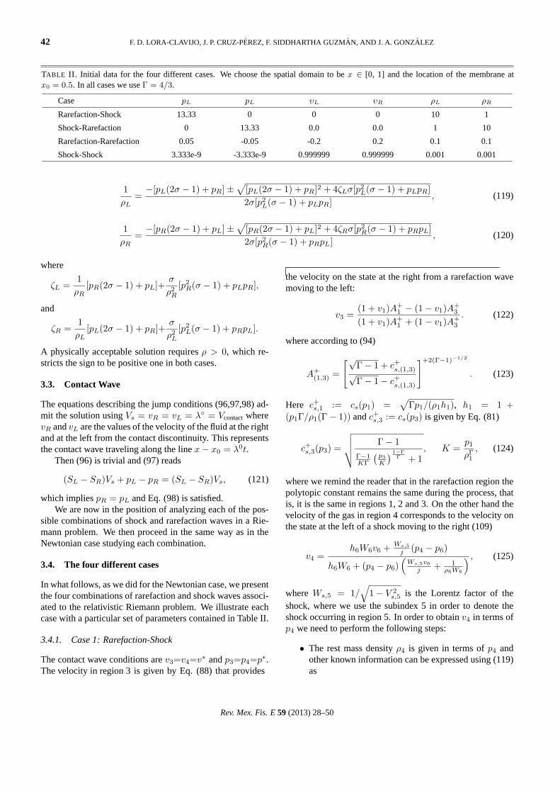
TABLE II. Initial data for the four different cases. We choose the spatial domain to bex ∈ [0, 1] and the location of the membrane atx0 = 0.5. In all cases we useΓ = 4/3.
Case pL pL υL υR ρL ρR
Rarefaction-Shock 13.33 0 0 0 10 1
Shock-Rarefaction 0 13.33 0.0 0.0 1 10
Rarefaction-Rarefaction 0.05 -0.05 -0.2 0.2 0.1 0.1
Shock-Shock 3.333e-9 -3.333e-9 0.999999 0.999999 0.001 0.001
1ρL
=−[pL(2σ − 1) + pR]±
√[pL(2σ − 1) + pR]2 + 4ζLσ[p2
L(σ − 1) + pLpR]2σ[p2
L(σ − 1) + pLpR], (119)
1ρR
=−[pR(2σ − 1) + pL]±
√[pR(2σ − 1) + pL]2 + 4ζRσ[p2
R(σ − 1) + pRpL]2σ[p2
R(σ − 1) + pRpL], (120)
where
ζL =1
ρR[pR(2σ − 1) + pL]+
σ
ρ2R
[p2R(σ − 1) + pLpR],
and
ζR =1ρL
[pL(2σ − 1) + pR]+σ
ρ2L
[p2L(σ − 1) + pRpL].
A physically acceptable solution requiresρ > 0, which re-stricts the sign to be positive one in both cases.
3.3. Contact Wave
The equations describing the jump conditions (96,97,98) ad-mit the solution usingVs = vR = vL = λ◦ = VcontactwherevR andvL are the values of the velocity of the fluid at the rightand at the left from the contact discontinuity. This representsthe contact wave traveling along the linex− x0 = λ0t.
Then (96) is trivial and (97) reads
(SL − SR)Vs + pL − pR = (SL − SR)Vs, (121)
which impliespR = pL and Eq. (98) is satisfied.We are now in the position of analyzing each of the pos-
sible combinations of shock and rarefaction waves in a Rie-mann problem. We then proceed in the same way as in theNewtonian case studying each combination.
3.4. The four different cases
In what follows, as we did for the Newtonian case, we presentthe four combinations of rarefaction and shock waves associ-ated to the relativistic Riemann problem. We illustrate eachcase with a particular set of parameters contained in Table II.
3.4.1. Case 1: Rarefaction-Shock
The contact wave conditions arev3=v4=v∗ andp3=p4=p∗.The velocity in region 3 is given by Eq. (88) that provides
the velocity on the state at the right from a rarefaction wavemoving to the left:
v3 =(1 + v1)A+
1 − (1− v1)A+3
(1 + v1)A+1 + (1− v1)A+
3
. (122)
where according to (94)
A+(1,3) =
[√Γ− 1 + c+
s,(1,3)√Γ− 1− c+
s,(1,3)
]+2(Γ−1)−1/2
. (123)
Here c+s,1 := cs(p1) =
√Γp1/(ρ1h1), h1 = 1 +
(p1Γ/ρ1(Γ− 1)) andc+s,3 := cs(p3) is given by Eq. (81)
c+s,3(p3) =
√√√√ Γ− 1Γ−1KΓ
(p3K
) 1−ΓΓ + 1
, K =p1
ρΓ1
, (124)
where we remind the reader that in the rarefaction region thepolytopic constant remains the same during the process, thatis, it is the same in regions 1, 2 and 3. On the other hand thevelocity of the gas in region 4 corresponds to the velocity onthe state at the left of a shock moving to the right (109)
v4 =h6W6v6 + Ws,5
j (p4 − p6)
h6W6 + (p4 − p6)(
Ws,5v6j + 1
ρ6W6
) , (125)
where Ws,5 = 1/√
1− V 2s,5 is the Lorentz factor of the
shock, where we use the subindex 5 in order to denote theshock occurring in region 5. In order to obtainv4 in terms ofp4 we need to perform the following steps:
• The rest mass densityρ4 is given in terms ofp4 andother known information can be expressed using (119)as
Rev. Mex. Fis. E59 (2013) 28–50
EXACT SOLUTION OF THE 1D RIEMANN PROBLEM IN NEWTONIAN AND RELATIVISTIC HYDRODYNAMICS 43
1ρ4
=−[p4(2σ − 1) + p6] +
√[p4(2σ − 1) + p6]2 + 4ζ4σ[p2
4(σ − 1) + p4p6]2σ[p2
4(σ − 1) + p4p6], (126)
ζ4 =1ρ6
[p6(2σ − 1) + p4] +σ
ρ26
[p26(σ − 1) + p4p6], whereσ =
ΓΓ− 1
. (127)
• Onceρ4 is given in terms ofp4 it is possible to computethe enthalpy in region 4 ash4 = 1 + σ(p4/ρ4).
• Then Eq. (115) reads
j2 = − (p4 − p6)h4ρ4− h6
ρ6
, (128)
whereh6 = 1 + σ(p6/ρ6). Something to rememberhere is the fact that as the shock moves to the right, weconsiderj to be the positive square root.
• Oncej is obtained, the shock velocity can be foundfrom expression (111) as
Vs,5 =ρ26W
26 v6 + |j|
√j2 + ρ2
6
j2 + ρ26W
26
. (129)
• Finally one calculatesWs,5 = 1/√
1− V 2s,5 and in this
way v4 in terms ofp4 and the known state in region 6using (125).
According to the contact discontinuity conditionv3=v4=v∗, we equate (122) and (125) and obtain a tran-scendental equation forp∗:
(1 + v1)A+1 − (1− v1)A+
3 (p∗)(1 + v1)A+
1 + (1− v1)A+3 (p∗)
−
h6W6v6 + Ws
j (p∗ − p6)
h6W6 + (p∗ − p6)(
Wsv6j + 1
ρ6W6
) = 0, (130)
which has to be solved using a root finder.Once this equation is solved,p3 and p4 are automati-
cally known andv3 and v4 can be calculated using (122)and (125), respectively. It is possible to calculateρ3 usingthe fact that in the rarefaction zone the process is adiabaticand thenρ3 = ρ1(p3/p1)1/Γ. On the other hand we can alsocalculateρ4 using (126). With this information it is alreadypossible to construct the solution in the whole domain.
Up to this point we account with the known initial states(p1, v1, ρ1) and(p6, v6, ρ6), the solution in regions 3 and 4given by(p3, v3, ρ3) and(p4, v4, ρ4), andVs,5 which repre-sents the velocity of propagation of the shock 5. The exactsolution region by region is described next.
1. Region 1 is defined by the conditionx − x0 <tξh, where according to (90)ξh is the velocity ofthe head of the rarefaction wave traveling to the left
ξh = v1 − cs,1/1− v1cs,1. The values of the physicalvariables are known from the initial conditions:
pexact = p1, (131)
vexact = v1, (132)
ρexact = ρ1. (133)
2. Region 2 is defined by the conditiontξh < x − x0 <tξt, where according to (91)ξt is the characteristicvalue again, but this time evaluated at the tail of the rar-efaction wave, that isξt = (v3 − cs,3)/(1− v3cs,3).In order to computev2 we use (92)
1 + v1
1− v1A+
1 −1 + v2
1− v2A+
2 (v2) = 0 (134)
considering Eqs. (76), (94) and (95) as follows
A+(1,2) =
[√Γ− 1 + c+
s,(1,2)√Γ− 1− c+
s,(1,2)
]+2(Γ−1)−1/2
, (135)
c+s,1 =
√Γp1
ρ1h1, h1 = 1 +
p1
ρ1
(Γ
Γ− 1
)(136)
c+s,2 =
v2 − ξ
1− v2ξ⇒ v2 =
ξ + c+s,2
1 + c+s,2ξ
. (137)
whereξ = (x − x0)/t. In this way, Eq. (134) is tran-scendental and has to be solved equivalently forv2 orfor c+
s,2 using a root finder for each point of region 2.We recommend solving forc+
s,2 and then constructv2
using (137). Finally we calculateρ2 using Eq. (82):
ρ2 =1
[KΓ
(1
(c+s,2)
2 − 1Γ−1
)] 1Γ−1
, K =p1
ρΓ1
.
(138)Finally we obtainp2 using the fact that in the processK is constant
p2 = p1
(ρ2
ρ1
)Γ
. (139)
3. Region 3 is defined by the conditiontξt < x − x0 <tVcontact, whereVcontact = λo = v3 = v4. The solutionthere reads
Rev. Mex. Fis. E59 (2013) 28–50
44 F. D. LORA-CLAVIJO, J. P. CRUZ-PEREZ, F. SIDDHARTHA GUZMAN, AND J. A. GONZALEZ
pexact= p3, (140)
vexact= v3, (141)
ρexact= ρ3. (142)
4. Region 4 is defined by the conditiontVcontact < x −x0 < tVs,5, whereVs,5 is given by (129) and explicitly
pexact= p4, (143)
vexact= v4, (144)
ρexact= ρ4. (145)
5. There is no region 5. Only the shock traveling withspeedVs,5.
6. Region 6 is defined bytVs,5 < x − x0. In this regionthe solution is simply
pexact= p6, (146)
vexact= v6, (147)
ρexact= ρ6. (148)
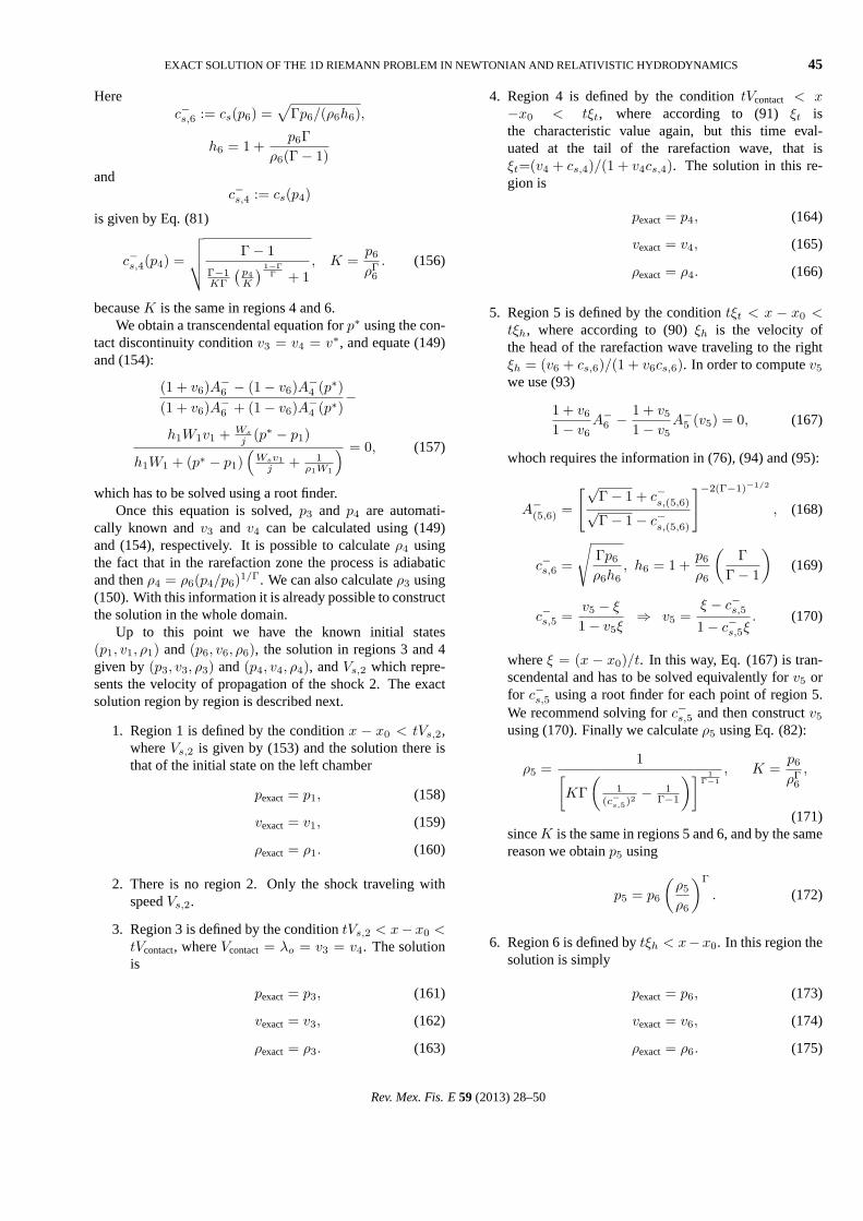
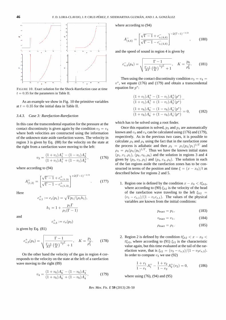
As an example we show in Fig. 9 the primitive variablesat t = 0.35 for the initial parameters in Table II.
3.4.2. Case 2: Shock-Rarefaction
This is pretty much the previous case, except that one has tobe careful at using the correct signs and conditions. We thenstart again with the contact wave conditionsv3 = v4 = v∗
FIGURE 9. Exact solution for the Rarefaction-Shock case at timet = 0.35 for the parameters in Table II.
andp3 = p4 = p∗. The velocity of the gas in region 3 cor-responds to the velocity on the state at the right from a shockmoving to the left (110)
v3 =h1W1v1 + Ws,2
j (p3 − p1)
h1W1 + (p3 − p1)(
Ws,2v1j + 1
ρ1W1
) , (149)
where Ws,2 = 1/√
1− V 2s,2 is the Lorentz factor of the
shock. In order to obtainv3 in terms ofp3 and other knowninformation we need to perform the following steps:
• The rest mass density is given in terms ofp3 using theexpression (120) as
1ρ3
=−[p3(2σ − 1) + p1] +
√[p3(2σ − 1) + p1]2 + 4ζ3σ[p2
3(σ − 1) + p3p1]2σ[p2
3(σ − 1) + p3p1], (150)
ζ3 =1ρ1
[p1(2σ − 1) + p3] +σ
ρ21
[p21(σ − 1) + p3p1], whereσ =
ΓΓ− 1
. (151)
• Onceρ3 is given in terms ofp3 it is possible to computethe enthalpy in region 3 ash3 = 1 + σ(p3/ρ3).
• Then from Eq. (115) we obtain
j2 = − (p3 − p1)h3ρ3− h1
ρ1
, (152)
whereh1 = 1 + σ(p1/ρ1). As the shock is movingto the left we consider the negative root of the aboveexpression forj.
• Oncej is obtained, the shock velocity can be foundfrom expression (112) in terms ofp3 as
Vs,2 =ρ21W
21 v1 − |j|
√j2 + ρ2
1
j2 + ρ21W
21
. (153)
• Finally one calculatesWs,2 = 1/√
1− V 2s,2 and in this
way v3 in terms ofp3 and the known state in region 1using (149).
The velocity in region 4 is given by Eq. (89) that pro-vides the velocity on the state at the left from a rarefactionwave moving to the right:
v4 =(1 + v6)A−6 − (1− v6)A−4(1 + v6)A−6 + (1− v6)A−4
, (154)
where following (94)
A−(4,6) =
[√Γ− 1 + c−s,(4,6)√Γ− 1− c−s,(4,6)
]−2(Γ−1)−1/2
. (155)
Rev. Mex. Fis. E59 (2013) 28–50
EXACT SOLUTION OF THE 1D RIEMANN PROBLEM IN NEWTONIAN AND RELATIVISTIC HYDRODYNAMICS 45
Herec−s,6 := cs(p6) =
√Γp6/(ρ6h6),
h6 = 1 +p6Γ
ρ6(Γ− 1)and
c−s,4 := cs(p4)
is given by Eq. (81)
c−s,4(p4) =
√√√√ Γ− 1Γ−1KΓ
(p4K
) 1−ΓΓ + 1
, K =p6
ρΓ6
. (156)
becauseK is the same in regions 4 and 6.We obtain a transcendental equation forp∗ using the con-
tact discontinuity conditionv3 = v4 = v∗, and equate (149)and (154):
(1 + v6)A−6 − (1− v6)A−4 (p∗)(1 + v6)A−6 + (1− v6)A−4 (p∗)
−
h1W1v1 + Ws
j (p∗ − p1)
h1W1 + (p∗ − p1)(
Wsv1j + 1
ρ1W1
) = 0, (157)
which has to be solved using a root finder.Once this equation is solved,p3 and p4 are automati-
cally known andv3 and v4 can be calculated using (149)and (154), respectively. It is possible to calculateρ4 usingthe fact that in the rarefaction zone the process is adiabaticand thenρ4 = ρ6(p4/p6)1/Γ. We can also calculateρ3 using(150). With this information it is already possible to constructthe solution in the whole domain.
Up to this point we have the known initial states(p1, v1, ρ1) and(p6, v6, ρ6), the solution in regions 3 and 4given by(p3, v3, ρ3) and(p4, v4, ρ4), andVs,2 which repre-sents the velocity of propagation of the shock 2. The exactsolution region by region is described next.
1. Region 1 is defined by the conditionx − x0 < tVs,2,whereVs,2 is given by (153) and the solution there isthat of the initial state on the left chamber
pexact = p1, (158)
vexact = v1, (159)
ρexact = ρ1. (160)
2. There is no region 2. Only the shock traveling withspeedVs,2.
3. Region 3 is defined by the conditiontVs,2 < x− x0 <tVcontact, whereVcontact = λo = v3 = v4. The solutionis
pexact = p3, (161)
vexact = v3, (162)
ρexact = ρ3. (163)
4. Region 4 is defined by the conditiontVcontact < x−x0 < tξt, where according to (91)ξt isthe characteristic value again, but this time eval-uated at the tail of the rarefaction wave, that isξt=(v4 + cs,4)/(1 + v4cs,4). The solution in this re-gion is
pexact = p4, (164)
vexact = v4, (165)
ρexact = ρ4. (166)
5. Region 5 is defined by the conditiontξt < x − x0 <tξh, where according to (90)ξh is the velocity ofthe head of the rarefaction wave traveling to the rightξh = (v6 + cs,6)/(1 + v6cs,6). In order to computev5
we use (93)
1 + v6
1− v6A−6 −
1 + v5
1− v5A−5 (v5) = 0, (167)
whoch requires the information in (76), (94) and (95):
A−(5,6) =
[√Γ− 1 + c−s,(5,6)√Γ− 1− c−s,(5,6)
]−2(Γ−1)−1/2
, (168)
c−s,6 =
√Γp6
ρ6h6, h6 = 1 +
p6
ρ6
(Γ
Γ− 1
)(169)
c−s,5 =v5 − ξ
1− v5ξ⇒ v5 =
ξ − c−s,5
1− c−s,5ξ. (170)
whereξ = (x − x0)/t. In this way, Eq. (167) is tran-scendental and has to be solved equivalently forv5 orfor c−s,5 using a root finder for each point of region 5.We recommend solving forc−s,5 and then constructv5
using (170). Finally we calculateρ5 using Eq. (82):
ρ5 =1
[KΓ
(1
(c−s,5)2 − 1
Γ−1
)] 1Γ−1
, K =p6
ρΓ6
,
(171)sinceK is the same in regions 5 and 6, and by the samereason we obtainp5 using
p5 = p6
(ρ5
ρ6
)Γ
. (172)
6. Region 6 is defined bytξh < x−x0. In this region thesolution is simply
pexact = p6, (173)
vexact = v6, (174)
ρexact = ρ6. (175)
Rev. Mex. Fis. E59 (2013) 28–50
46 F. D. LORA-CLAVIJO, J. P. CRUZ-PEREZ, F. SIDDHARTHA GUZMAN, AND J. A. GONZALEZ
FIGURE 10. Exact solution for the Shock-Rarefaction case at timet = 0.35 for the parameters in Table II.
As an example we show in Fig. 10 the primitive variablesat t = 0.35 for the initial data in Table II.
3.4.3. Case 3: Rarefaction-Rarefaction
In this case the transcendental equation for the pressure at thecontact discontinuity is given again by the conditionv3 = v4
where both velocities are constructed using the informationof the unknown state aside rarefaction waves. The velocity inregion 3 is given by Eq. (88) for the velocity on the state atthe right from a rarefaction wave moving to the left:
v3 =(1 + v1)A+
1 − (1− v1)A+3
(1 + v1)A+1 + (1− v1)A+
3
, (176)
where according to (94)
A+(1,3) =
[√Γ− 1 + c+
s,(1,3)√Γ− 1− c+
s,(1,3)
]+2(Γ−1)−1/2
. (177)
Herec+s,1 := cs(p1) =
√Γp1/(ρ1h1),
h1 = 1 +p1Γ
ρ1(Γ− 1)
andc+s,3 := cs(p3)
is given by Eq. (81)
c+s,3(p3) =
√√√√ Γ− 1Γ−1KΓ
(p3K
) 1−ΓΓ + 1
, K =p1
ρΓ1
. (178)
On the other hand the velocity of the gas in region 4 cor-responds to the velocity on the state at the left of a rarefactionwave moving to the right (89)
v4 =(1 + v6)A−6 − (1− v6)A−4(1 + v6)A−6 + (1− v6)A−4
, (179)
where according to (94)
A−(4,6) =
[√Γ− 1 + c−s,(4,6)√Γ− 1− c−s,(4,6)
]−2(Γ−1)−1/2
, (180)
and the speed of sound in region 4 is given by
c−s,4(p4) =
√√√√ Γ− 1Γ−1KΓ
(p4K
) 1−ΓΓ + 1
, K =p6
ρΓ6
. (181)
Then using the contact discontinuity conditionv3 = v4 =v∗, we equate (176) and (179) and obtain a transcendentalequation forp∗:
(1 + v1)A+1 − (1− v1)A+
3 (p∗)(1 + v1)A+
1 + (1− v1)A+3 (p∗)
−
(1 + v6)A−6 − (1− v6)A−4 (p∗)(1 + v6)A−6 + (1− v6)A−4 (p∗)
= 0, (182)
which has to be solved using a root finder.Once this equation is solved,p3 andp4 are automatically
known andv3 andv4 can be calculated using (176) and (179),respectively. As in the previous two cases, it is possible tocalculateρ3 andρ4 using the fact that in the rarefaction zonethe process is adiabatic and thenρ3 = ρ1(p3/p1)1/Γ andρ4 = ρ6(p4/p6)1/Γ. Thus we have the known initial states(p1, v1, ρ1), (p6, v6, ρ6) and the solution in regions 3 and 4given by (p3, v3, ρ3) and (p4, v4, ρ4). The solution in eachof the fan regions aside the rarefaction zones has to be con-structed in terms of the position and timeξ = (x − x0)/t asdescribed below for regions 2 and 5.
1. Region one is defined by the conditionx− x0 < tξh2,where according to (90)ξh2 is the velocity of the headof the rarefaction wave traveling to the leftξh2 =(v1 − cs,1)/(1− v1cs,1). The values of the physicalvariables are known from the initial conditions:
pexact= p1, (183)
vexact= v1, (184)
ρexact= ρ1. (185)
2. Region 2 is defined by the conditiontξh2 < x− x0 <tξt2, where according to (91)ξt2 is the characteristicvalue again, but this time evaluated at the tail of the rar-efaction wave, that isξt2 = (v3 − cs,3)/(1− v3cs,3).In order to computev2 we use (92)
1 + v1
1− v1A+
1 −1 + v2
1− v2A+
2 (v2) = 0, (186)
where using (76), (94) and (95)
Rev. Mex. Fis. E59 (2013) 28–50

EXACT SOLUTION OF THE 1D RIEMANN PROBLEM IN NEWTONIAN AND RELATIVISTIC HYDRODYNAMICS 47
A+(1,2) =
[√Γ− 1 + c+
s,(1,2)√Γ− 1− c+
s,(1,2)
]+2(Γ−1)−1/2
, (187)
c+s,1 =
√Γp1
ρ1h1, h1 = 1 +
p1
ρ1
(Γ
Γ− 1
)(188)
c+s,2 =
v2 − ξ
1− v2ξ⇒ v2 =
ξ + c+s,2
1 + c+s,2ξ
. (189)
whereξ = (x − x0)/t. In this way, Eq. (186) is tran-scendental and has to be solved equivalently forv2 orfor c+
s,2 using a root finder for each point of region 2.We solve forc+
s,2 and constructv2 using (189). Finallywe calculateρ2 using Eq. (82):
ρ2 =1
[KΓ
(1
(c+s,2)
2 − 1Γ−1
)] 1Γ−1
,
K =p1
ρΓ1
. (190)
Finally we obtainp2 using
p2 = p1
(ρ2
ρ1
)Γ
. (191)
3. Region 3 is defined by the conditiontξt2 < x − x0 <tVcontact, whereVcontact = λo = v3 = v4. The solutionthere reads
pexact = p3, (192)
vexact = v3, (193)
ρexact = ρ3. (194)
4. Region 4 is defined by the conditiontVcontact < x −x0 < tξt5, whereξt5 is the third characteristic valuecalculated at the tail of rarefaction moving to the right,and according to (91)ξt5 = (v4 + cs,4)/(1 + v4cs,4).In this region thus
pexact = p4, (195)
vexact = v4, (196)
ρexact = ρ4. (197)
5. Region 5 is defined by the conditiontξt5 < x − x0 <tξh5, whereξh5 = (v6 + cs,6)/(1 + v6cs,6) accordingto (90). In order to computev5 we use (93)
1 + v5
1− v5A−5 (v5)− 1 + v6
1− v6A−6 = 0, (198)
where according to (76), (94) and (95)
A−(5,6) =
[√Γ− 1 + c−s,(5,6)√Γ− 1− c−s,(5,6)
]−2(Γ−1)−1/2
, (199)
c−s,6 =
√Γp6
ρ6h6, h6 = 1 +
p6
ρ6
(Γ
Γ− 1
), (200)
c−s,5 = − v5 − ξ
1− v5ξ⇒ v5 =
ξ − c−s,5
1− c−s,5ξ, (201)
whereξ = (x−x0)/t. Again (198) is a transcendentalequation either forv5 or for c−s,5. Oncec−s,5 has beencalculated use (201) to constructv5 or directly solve(198) forv5. It is possible to calculateρ5 using (82):
ρ5 =1
[KΓ
(1
(c−s,5)2 − 1
Γ−1
)] 1Γ−1
, K =p6
ρΓ6
,
(202)and finally the pressure
p5 = p6
(ρ5
ρ6
)Γ
. (203)
6. Region 6 is defined bytξh5 < x − x0. In this regionthe solution is simply
pexact = p6, (204)
vexact = v6, (205)
ρexact = ρ6. (206)
As an example we show in Fig. 11 the primitive variablesat t = 0.25, for the initial parameters in Table II.
FIGURE 11. Exact solution for the Rarefaction-Rarefaction case attime t = 0.25 for the parameters in Table II.
Rev. Mex. Fis. E59 (2013) 28–50
48 F. D. LORA-CLAVIJO, J. P. CRUZ-PEREZ, F. SIDDHARTHA GUZMAN, AND J. A. GONZALEZ
3.4.4. Shock-Shock
We proceed as always, by establishing a relationship betweenthe velocity in regions 3 and 4. We start by expressingv3 asthe velocity of the gas on a region at the right from a shockmoving to the left, that is, according to (110)
v3 =h1W1v1 + Ws,2
j2(p3 − p1)
h1W1 + (p3 − p1)(
Ws,2v1j2
+ 1ρ1W1
) , (207)
where Ws,2 = 1/√
1− V 2s,2 is the Lorentz factor of the
shock moving to the left. In this particular case we dis-tinguish between the two values ofj depending using thesubindices 2 and 5. In order to obtainv3 in terms ofp3 wecan proceed following these steps:
• The rest mass density is given in terms ofp3 using theexpression (120) as
1ρ3
=−[p3(2σ − 1) + p1] +
√[p3(2σ − 1) + p1]2 + 4ζ3σ[p2
3(σ − 1) + p3p1]2σ[p2
3(σ − 1) + p3p1], (208)
ζ3 =1ρ1
[p1(2σ − 1) + p3] +σ
ρ21
[p21(σ − 1) + p3p1], whereσ =
ΓΓ− 1
. (209)
• Onceρ3 is given in terms ofp3 it is possible to computeenthalpy in region 3 ash3 = 1 + σ(p3/ρ3).
• Then from Eq. (115) we obtain
j22 = − (p3 − p1)
h3ρ3− h1
ρ1
, (210)
where we choosej2 to be the negative root since theshock is moving to the left; hereh1 = 1 + σ(p1/ρ1).
• Oncej2 is obtained, the shock velocity can be foundfrom expression (112) in terms ofp3 as
Vs,2 =ρ21W
21 v1 − |j2|
√j22 + ρ2
1
j22 + ρ2
1W21
. (211)
• Finally we calculateWs,2 = 1/√
1− V 2s,2 and thusv3
in terms ofp3 and the known state in region 1 using(207).
Using the information of the shock moving to the rightwe obtain the velocity at the left from the shock, that isv4
using (109)
v4 =h6W6v6 + Ws,5
j5(p4 − p6)
h6W6 + (p4 − p6)(
Ws,5v6j5
+ 1ρ6W6
) , (212)
where Ws,5 = 1/√
1− V 2s,5 is the Lorentz factor of the
shock. In order to obtainv4 in terms ofp4 we need to performthe following steps:
• The rest mass density is given in terms ofp4 using theexpression (119) as
1ρ4
=−[p4(2σ − 1) + p6] +
√[p4(2σ − 1) + p6]2 + 4ζ4σ[p2
4(σ − 1) + p4p6]2σ[p2
4(σ − 1) + p4p6], (213)
ζ4 =1ρ6
[p6(2σ − 1) + p4] +σ
ρ26
[p26(σ − 1) + p4p6], where σ =
ΓΓ− 1
. (214)
• Onceρ4 is given in terms ofp4, we are able to computeenthalpy in region 4 ash4 = 1 + σ(p4/ρ4).
• Then Eq. (115) reads
j25 = − (p4 − p6)
h4ρ4− h6
ρ6
, (215)
hereh6 = 1+σ(p6/ρ6). In this case, since the shock ismoving to the right we choose thej5 to be the positiveroot.
• Oncej5 is obtained, the shock velocity can be foundfrom expression (111)
Vs,5 =ρ26W
26 v6 + |j5|
√j25 + ρ2
6
j25 + ρ2
6W26
. (216)
• Finally we calculateWs,5 = 1/√
1− V 2s,5 and in this
way we can obtainv4 in terms ofp4 with (212) and theknown state in region 6.
According to the contact discontinuity conditionv3 =v4 = v∗, we equate (207) and (212) and obtain a transcen-dental equation forp∗:
Rev. Mex. Fis. E59 (2013) 28–50
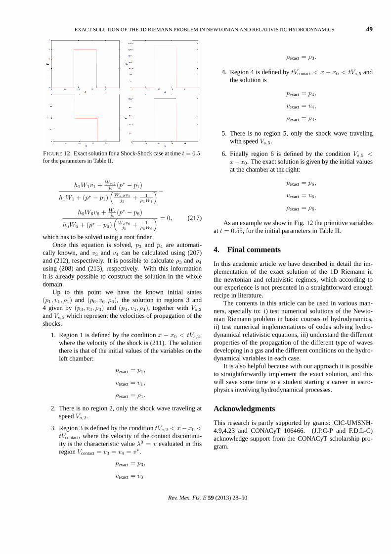
EXACT SOLUTION OF THE 1D RIEMANN PROBLEM IN NEWTONIAN AND RELATIVISTIC HYDRODYNAMICS 49
FIGURE 12. Exact solution for a Shock-Shock case at timet = 0.5
for the parameters in Table II.
h1W1v1 + Ws,2j2
(p∗ − p1)
h1W1 + (p∗ − p1)(
Ws,2v1j2
+ 1ρ1W1
)−
h6W6v6 + Ws
j5(p∗ − p6)
h6W6 + (p∗ − p6)(
Wsv6j5
+ 1ρ6W6
) = 0, (217)
which has to be solved using a root finder.Once this equation is solved,p3 and p4 are automati-
cally known, andv3 and v4 can be calculated using (207)and (212), respectively. It is possible to calculateρ3 andρ4
using (208) and (213), respectively. With this informationit is already possible to construct the solution in the wholedomain.
Up to this point we have the known initial states(p1, v1, ρ1) and (p6, v6, ρ6), the solution in regions 3 and4 given by(p3, v3, ρ3) and (p4, v4, ρ4), together withVs,2
andVs,5 which represent the velocities of propagation of theshocks.
1. Region 1 is defined by the conditionx − x0 < tVs,2,where the velocity of the shock is (211). The solutionthere is that of the initial values of the variables on theleft chamber:
pexact = p1,
vexact = v1,
ρexact = ρ1.
2. There is no region 2, only the shock wave traveling atspeedVs,2.
3. Region 3 is defined by the conditiontVs,2 < x− x0 <tVcontact, where the velocity of the contact discontinu-ity is the characteristic valueλ0 = v evaluated in thisregionVcontact= v3 = v4 = v∗.
pexact = p3,
vexact = v3
ρexact = ρ3.
4. Region 4 is defined bytVcontact < x − x0 < tVs,5 andthe solution is
pexact = p4,
vexact = v4,
ρexact = ρ4.
5. There is no region 5, only the shock wave travelingwith speedVs,5.
6. Finally region 6 is defined by the conditionVs,5 <x−x0. The exact solution is given by the initial valuesat the chamber at the right:
pexact = p6,
vexact = v6,
ρexact = ρ6.
As an example we show in Fig. 12 the primitive variablesat t = 0.55, for the initial parameters in Table II.
4. Final comments
In this academic article we have described in detail the im-plementation of the exact solution of the 1D Riemann inthe newtonian and relativistic regimes, which according toour experience is not presented in a straightforward enoughrecipe in literature.
The contents in this article can be used in various man-ners, specially to: i) test numerical solutions of the Newto-nian Riemann problem in basic courses of hydrodynamics,ii) test numerical implementations of codes solving hydro-dynamical relativistic equations, iii) understand the differentproperties of the propagation of the different type of wavesdeveloping in a gas and the different conditions on the hydro-dynamical variables in each case.
It is also helpful because with our approach it is possibleto straightforwardly implement the exact solution, and thiswill save some time to a student starting a career in astro-physics involving hydrodynamical processes.
Acknowledgments
This research is partly supported by grants: CIC-UMSNH-4.9,4.23 and CONACyT 106466. (J.P.C-P and F.D.L-C)acknowledge support from the CONACyT scholarship pro-gram.
Rev. Mex. Fis. E59 (2013) 28–50
50 F. D. LORA-CLAVIJO, J. P. CRUZ-PEREZ, F. SIDDHARTHA GUZMAN, AND J. A. GONZALEZ
1. E. F. Toro,Riemann solvers and numerical methods for fluiddynamics.(Springer-Verlag Berlin-Heidelberg, 2009).
2. J. Ma. Martı, E. Muller, Living Rev. Relativity6 (2003) 7.http://www.livingreviews.org/lrr-2003-7
3. J. Ma. Martı, E. Muller, J. Fluid. Mech.258(1994) 317-333.
4. R. J. LeVeque, inNumerical methods for conservation laws.(Birkhauser, Basel, 1992).
5. G. A. Sod,J. Comp. Phys.27 (1978) 1-31.
6. A. Taub,Phys. Rev.74 (1948) 328-334.
7. K. S. Thorne,Astrophys. J.179(1973) 897-907.
Rev. Mex. Fis. E59 (2013) 28–50
Related Documents