Exact Controllability of the Euler-Bernoulli Equation with L2 (Σ)-control Only in the Dirichlet Boundary Conditions

JOURNAL OF MATHEMATICAL ANALYSIS AND APPLICATIONS 146, 1-33 (1990)

Exact Controllability of the Euler-Bernoulli Equation with Boundary Controls for Displacement and Moment*

I. LASIECKA AND R. TRIGGIANI

Department of Applied Mathematics, Thornton Hall, University of Virginia, CharlottesviNe, Virginia 22903

Submitted by A. Schumit:k>

Received January 29, 1988

Contents. 1. Introduction, statement of main results, literature. 2. Proof of Theorem 1.1: Exacf controllabilily for any T>O on [D(A14)]‘x

[D(A3”)]’ wifh g, E L’(L) and gzE [H’(O, T; Z,‘(r))]‘. 3. Proof of Theorem 1.2: Exact controllability for any T> 0 on D(A”“) x [D(A”“)]’

with g, E Hi(O, T; L2(r)) and g, E L’(L). Corollary 1.3. Appendix A : Proof of identity (2.1). Appendix B: Proof of identity (2.34).

We consider the Euler-Bernoulli problem (1.1) in the solution u(r, .) with boundary controls g, and g, acting in the Dirichlet traces for ns and dw, respectively. We show two main exact controllability results both in the spaces of maximal regularity of the solution at f= T (see I. Lasiecka and R. Triggiani, Regularity theory for a class of Euler Bernoulli equations: a cosine operator approach, Boll. Unione Mat. Ital. j7). 3-B (1989)) and both withour geometrical conditions on the open bounded domain Q (except for smoothness of its boundary r): one with g, E L2(0, T, L*(r)) and g, E [H’(O, T; L’(f))] for any T> 0 arbitrarily short; and one with g, E HA(O, T, L*(r)) and g, E L2(0, r; L’(T)) for all 7’> 0 sufficiently large. An interpolation result between these two cases is also presented. A direct approach is given based on two main steps. First, by means of an operator model (I. Lasiecka and R. Triggiani, Regularity theory for a class of Euler Bernoulli equations: a cosine operator approach, Boll. Unione Mar. Ital. (7/, 3-B (1989).) for problem (1.1) and a functional analytic approach, the question of exact controllability is shown to be equivalent to an a-priori inequality for the corresponding homogeneous problem. Next, this a-priori inequality is proved to hold true by means of multiplier techniques. These are inspired by recent progress on the maximal regularity, exact controllability and uniform stabilization questions for second order hyperbolic equations. c 1990 Academic Press, Inc.

* Research partially supported by National Science Foundation under Grant DMS-87- 96320 and by Air Force Office of Scientific Research under Grant AFOSR-87-0321. A preliminary version of this paper has appeared in Topics in Mathematical Analysis, Series in Pure Mathematics, Vol. II, T. M. Rassias, Ed.. World Scientific, 1989, pp. 576622.

1 0022-247X/90 $3.00

Copyright r‘ 1990 by Academic Press, Inc. All rights of reproduction in any form reserved.

2 LASIECKA AND TRIGGIANI

1. INTRODUCTION, STATEMENT OF MAIN RESULTS. LITERATURE

Throughout this paper n is an open bounded domain in R”, typically n > 1, with sufficiently smooth boundary SSZ = r, see Remark 1.2. In a we consider the following non homogeneous problem for the Euler-Bernoulli equation in the solution n(t, x):

w,, + A % = 0 in (0, T] x Sz = Q (l.la)

w(0, . ) = 1r.O; w, ((0, . ) = w ’ in Sz (lib)

M’I z=g1 in (0, T] x f = ,Y (l.lc)

Awl,= g2 in z (l.ld)

with control functions g,, g,. The regularity question for problem ( 1.1) was recently studied in [L-T.81, whose major results (relevant to the present paper) will be recalled below as Theorem 1.0. The aim of this article is to study the exact controllability question for (1.1). Qualitatively this means: given n, we ask whether there exists some To > 0, such that if T> To, the following steering property of (1.1) holds true: for all initial data M”, ujl in some preassigned space 2 = Z, x Z, based on 52, there exist suitable control functions g, and g, on some preassigned space Vz = Vi, x V,, based on TX (0, T], whose corresponding solution of ( 1.1) satisfies w( T, .) = 0, M’,( T, .) = 0. We then say that the dynamics (1.1) is exactly controllable on the space Z over the interval [0, T] by means of control functions in VI. We shall consider a few natural choices of pairs [Z, V,] of spaces. In fact, these will be selected according to the regularit? results established in [L-T.81. In order to report these results, we need to introduce some preliminary background. Throughout the paper we let A : L2(a) 3 D(A) + L2(s2) be the positive, self-adjoint operator defined by

Ah=d2h,D(A)={h~L2(SZ):dZh~L2(Q),h~.=dh~,-=O}

= {hM4(Q): hI,=dhI,-=O}. (1.2

It is expedient to record the known result that

‘4’12 = A,, (1.3

where A, is the (positive, self-adjoint) operator defined by

A,h = -Ah, W~A=~,WV-J~:,W) (1.4)

the subscript “D” reminding us that A, has homogeneous boundary conditions of Dirichlet type. The following space identifications are known (with equivalent norms) [G. 1 ] [L-M. I]

EULER-BERNOULLI EQUATION 3

II = {hEH4e(Q): hl,=O) = H;e(sz), $<O<i (1.5)

II( (hEH4e(Q):hJr=dhlr=0}, $<O<l. (1.6)

The following specialization thereof will be needed below

6 = $: D(A’14) = HA(G) (with equivalent norms); for fe HA(Q) (1.7a)

norm lifll D(Al141 - IIA “4fll L~u2) equivalent to llfll Hi, in turn equivalent to the gradient-norm (1.7b)

{r, l?fl’dQ)“‘, by Poincare inequality.

0 = a: D(,4”“) = V (with equivalent norms)

v= {hEH3(Q):hI,=dhIr=0} (1.8a)

norm llfll o~A~~4~ = IIA3’4flI L2cRI = IA 1’4~DfllLq~~ = IV ““W)lL l/2 (1.8b)

equivalent to {I

lV(Af)l’ dQ , by (1.7b). a I

In general, natural norms are

ll~ll~~aa, = [email protected] Lqn); l/xl/ cD(~/ol, = UA -‘XII LW) (1.9)

for /?>O, where [D(AO)] denotes the dual space of D(Ap) with respect to the L’(R)-topology.

THEOREM 1.0 (Regularity [L-T.81). (i) C onsider problem ( 1.1) subject to’

{ w”, w’} E [D(A”4)]’ x [D(A3”)]’ = H-‘(Q) x V (1.10)

g, E L”(L’), g, E [H’(O, T; L2(Z-))I’. (1.11)’

Then the map

{ WO, w’, g,, g2) + {W(T), W,(T)}EH~‘(52)x V’ (1.12)

is continuous. Moreover, the map

{d, Iv’, g,, g2) -+ {u’(t), w,(t)> (1.13a)

’ [H’(O, T; L'(F))]' is the space dual to H’(0, T; L*(f)) with respect to the H’(0, T; L2(F))- topology. Since HA(O, T; L*(r)) 5 H’(0, T; L2(F), we then have [H’(O, T; L’(T))]’ 5 H-'(0, T; L*(f)).

4 LASIECKA AND TRIGCIANI

is likewise continuous into

C([O, T]; H ‘(i-2)) x L’(0. T; V’),

u)here L’ in (1.13b) cannot be replaced by, C

(ii) Consider problem ( 1.1) subjecr to

i WO, W’)ED(A’14)X [D(A”4)]‘=H(#2)xH -l(Q)

g, E H;(O, T; L*(Z)); g, E L’(E).

Then the map

{ w”, II”, g,,g,}~{u’(T),w,(T)}EH~(n)xH~‘(R)

is continuous. Moreover, the map

{ U’O, WI* g,. g*> + iw(t)t w,(t))

is continuous into

(1.13b)

(1.14)

(1.15)

(1.16)

(1.17a)

CCC& Tl; H”*(SZ)b U[lO, 7-I; H- ‘U-2)), (1.17b)

where H”*(Q) cannot be replaced by HA(Q).

We can now state our main exact controllability results. They do not require geometrical conditions on a.

THEOREM 1.1 (Exact controllability on [D(A”4)]’ x [D(A3’4)]’ = H-‘(Q) x V’). For any T> 0, given any pair of initial data

{U-O, w’) E [D(A”4)]‘x [D(FI~‘~)]‘= H-‘(Q) x V’ (1.18)

there exist boundary controls

g, E L”(Z); g, E [H’(O, T; L’(r))]’

such that the corresponding solution to problem (1.1) satisfies

w(T)=wt(T)=O

as wefl as (1.13).

(1.19)

(1.20)

THEOREM 1.2 (Exact controllability on D(A ‘j4) x [D(A “4)]’ = HA(Q) x H-‘(Q)). For any T>O given any initial data

i w”, w’) ED(A”~)x [D(A1’4)]‘= H;(Q) x H-‘(Q) (1.21)

EULER-BERNOULLI EQUATION

there exist boundary controls

g, E fJ;(O, T; L’(r)); g, E L2W

such that the corresponding solution to problem (1.1) satisfies

w(T)=wt(T)=O

as well as (1.17). [

Remark 1.1. Consider the following homogeneous problem

d,, + A24 = 0 in Q

~I,=0=~“~~,I,=0=4’ in Q

#I==0 in C

4l,=O in C.

(1.22)

(1.23)

(1.24a)

(1.24b)

(1.24~)

(1.24d)

The proof of Theorem 1.1 shows that exact controllability as stated there is equioalent to the following inequality: there is C;>O such that for all {q3”, q5’} E D(A3j4) x D(A ‘14) we have

j,(~)2+(~)2+(~)2d~bC;,,{mo,m’}l16,,34,,.,,i~4, (1.25)

see the (backward in time) problem (2.18) in Lemma 2.1. Next, Lemma 2.4 and Remark 2.1 at the end of Section 2 yield that inequality (1.25) is in fact equivalent to the following inequality: there is Cp> 0 such that for all {#“, c$‘} ED(A~/~) x D(A1’4) we have

i.e., the lower order term on ad/& can be absorbed by the other boundary terms. Finally, Proposition 2.2 shows that inequality (1.26) always holds true for any T> 0 and with no geometrical conditions on s2 (except for smoothness of Q as in Remark 1.2 below).

On the other hand, the opposite inequality

is likewise always true for all T> 0 [L-T.81. Thus, for any T> 0

(1.28)

6 LASIECKA AND TRIGGIAlSl

defines a norm on the space D(AJ4) x D(A’ “)= J’x H/,(Q), which is equivalent to the norm

llj~~~~1~lID,.4~J,~~,.4~J) ( 1.29 )

so that J. L. Lions’space Fin IL.21 is F=D(A3’4)~D(A”4)= VxHh(Q).

By interpolation between Theorem 1.1 and Theorem 1.2 we obtain part (ii) of the next corollary.

COROLLARY 1.3. (i) For any T > 0, inequality (2.21) [which characterizes exact controllability ofproblem (1.1) with g, E L*(C), g, E [H’(O, T;L’(T)] c H-‘(0, T;L’(T)) on the space [D(A1’4)]‘x [D(A3’4)]’ over [0, T]] and inequality (3.10) [which characterizes exact controllability of problem ( 1.1) with g,E HA(O, T; L’(r)), g, E L’(C) on the space D(A”4) x [D(A 1’4)]’ over [0, T]] are equivalent conditions.

(ii) When part (i) holds, we deduce by interpolation [ L-M.1, p. 29, 64-663, that problem (1 .l ) with controls

g, E H:, “(0, T; L*(r)), 0<8<1,B#$

g, E H,$(O, T; L’(T)), 6=$ (1.30)

g, E [H”(O, T; L’(T))]‘, 0<0<1, (1.31)

is exactly controllable on the space

W l/4 02) x D(A I,‘4 “,‘2), (1.32)

where we are using the convention that

D(A-“), /I 3 0 means [D(A”)]‘.

Remark 1.2 (On the smoothness of r). The proofs given below require the existence of a dense set of initial data for which the solutions of the correspondding homogeneous problem (1.24) possess the regularity required to carry out the actual computations in the multiplier methods of Sections 2-3. This condition is satisfied if r is sufficiently smooth.

Remark 1.3. Once exact controllability is established, then an elemen- tary argument provides the minimal norm, steering control (see the abstract operator argument in CT.2, Appendix B], [L-T.3, Appendix B] and its specialization there to the wave equation, as well as [L-T.7, Appendix D; L.61 and its specialization to plate problems).

Literature. This paper is part of the present effort on exact controllability problems for “plate equations,” which has followed the recent progress and understanding on questions of maximal regularity [L.l; L-T.2; L-T.4; L-L-T.11, uniform stabilization [LS; L-T.11 and exact controllability for second order hyperbolic equations CL.2; L.3; H.l;


K.1; T.21. (See also [F-L-T.11; [L-TS], for Riccati equations corresponding to these problems].) Here, for the Euler-Bernoulli problem (l.l), we pursue the same general direct “ontoness” approach to exact controllability which we have already carried out for (i) second order hyperbolic equations with Dirichlet CT.23 or Neumann CL-T.31 boundary control, and also for (ii) Euler-Bernoulli problems with different types of boundary conditions [L-T.6; L-T.71. Remark 1.3 then provides an explicit steering control, in fact the minimal-norm control. This is the one used by J. L. Lions in his approach. Our Theorem 1.1 is slightly stronger than a similar result sketched by J. L. Lions in CL.21 in the sense that in our present paper the boundary control g, is taken in the strictly smaller space [H’(O, T; L*(T))]’ than the space HP’(0, T; L*(r)) considered in [L.2]. Moreover, the approach in CL.21 and our present ontoness approach are different. Theorem 1.2 and the interpolation result Corollary 1.3 are new. Theorem 1.2 passes through a new feature (the term K,, in the boundary integral of the characterizing inequality (3.10) which is not encountered in second order hyperbolic equations or in the plate problems considered in [L.2]). It is not surprising that our exact controllability results are achieved for any T arbitrarily small [L-T.71, [Z.l]. For other work on plate equations we refer to CL-L.1 ] for different boundary conditions and to CL.41 for smoother spaces.

2. PROOF OF THEOREM 1.1: EXACT CONTROLLABILITY ON

[D(F!'/~)]'x [D(FI~/~)]' (COROLLARY 1.3)

Throughout this section we set for convenience

z= [D(A”4)]’ x [D(A3’4)]‘; u= L*(c) x [H’(O, T; L*(r))]‘, (2.0a)

where for .r= [y,, y2], z= [zl,z2 ] in Z, the inner product in Z is defined by

(y,z&=(A-1’4yl,A-1’4z1)L~~Q~+(A-3’4?,2, A-3’4z2),z0,. (2.0b)

The inner product on [H’(O, T; L2(f))] is defined as follows. Let ,4 be an isomorphism H’(0, T; L2(r)) + H’(O, T; L*(f)), self-adjoint on H’(O, T; L*(r)). Then

(“6 g)“~,o.T:Lw), = (4L 4)Lqo, T;L*(r))

(.L g)cH1(o,T:Lqr,)]’ = (A -tr, A %L2,0. T:L2(I-)).

Moreover from (2.0~)

(2.Oc)

(2.0d)

Ilfll2H’,O,T;L~~r~)- Ilfll2Lqz,+ f’ 7 II II = Il4ll L(Z). (2.0e)

L’G’)

8 LASIECKA AND TRIGtiIANI

Step 0. In line with the authors’ approach to time invariant problems for second order and fourth order differential operators in the space variables [L-T.l-L-T.81, we recall that the solution at time T to problem (1.1) with M” = W” =0 may be written explicitly as (see [L-T.8)):

[

w(T; t=O;wO=O, wJ=O)

,v,(T; t=O;wO=O, d=O) 1 = L,,g, + L,,g, = LT gl L 1 (2.1) g2

I T

A S(T- 1) G, g,(t) dt 0

L,Tg,=

s

T

A C(T-- t) G, g,(t) dt 0

(2.2)

S(T-

C(T-

t)

t)

G,g,(t)dt

G,gz(t) dt (2.3 )

Here, -A is the (negative self-adjoint) operator defined in (1.2) which generates a S.C. cosine operator C(t) on L’(Q), with S(t) = St, C(r) dq t E R. Moreover, G, and G, are Green maps defined as follows:

{

A’y=O in D

Glgl=.v- .vlr=g, on f (2.4) AJJ 1 r = 0 on I-

G,g,=v-= ylr=O

i

A2y=0 in 52 on r (2.5)

AA,-= g, on r.

By elliptic theory we have for any s E R [L-M.l, Vol. I, p. 188-1891

G, : continuous H”(r) + H” + ‘I’( 0) (2.6)

G,: continuous H”(T) + H”f5’2(.Q). (2.7)

Let now Gy be the adjoint of Gi in the sense

(Gig, 0) 2 ,c cn, = (g, G$),qr), g E L’(r), u E L2(Q). (2.8)

The following Lemma can be established by use of Green’s second theorem for its parts (ii), (iii).


LEMMA 2.0 [L-T.81. We haoe

6)

G,=D: G2= -A,‘D, (2.9)

where A, = A”*, see (1.3), and where

Dg=[oA<=O in Q; ( = g on C (2.10

(ii)

G:AfzD*AZ,f=y, f ED(A) (2.11

GfAL:y=D.,J=$f, f c D(A”*); (2.12)

(iii)

v G:Af = -D*A,f =%, f~ D(A1’2). (2.13)

Step 1. The (regularity) Theorem 1 .O gives that (recall (2.0a))

L,- C.&T, LIT]: continuous U --) 2 (2.14)

By time reversibility of problem (1.1 ), exact controllability of problem (1.1) on the space 2 over [0, r] by means of controls in U is equivalent to the condition that L;*: has a continuous inverse, i.e., [T-L.]] there is C,> 0 such that

(2.15)

for all z = [zt , z2] E 2, where for [g,, gz] E U

= (L,, g, + L,, g,, z)z

= (g,, L:Tz)L2(z,+ (g2, GTdCH~(O. T;L?r,,l,

(2.16a)

2 ; IlL~zll:, = llL~At2(r, -t llGT4 ;H1,0. 7-; L*(r),] (2.16b)

\\L;z\\:= \/L:,zl\2,2,,,+ ll~-%T42~,Z) (2.16c)

recalling (2.0d).


Step 2. An equivalent partial differential equation characterization of inequality (2.15) is given by the following Lemma.

LEMMA 2.1. For ,-EZ= [D(A”‘)]‘x [D(A3’“)]’ we have:

(i) Let

(L?+)(t) = v on z, (2.17)

where 4(t) = d(t, do, 4’) is the solution of the following homogeneous problem, backward in time

~,,+A’~-0 in Q (2.18a)

~It=T=~O;d,I~=T=~’ in Sz (2.18b)

41.X-0 in .Z (2.18~)

A4l,=O in C (2.18d)

with

(p=A-3”z,E~(A3/4); f$, = -A-‘:‘z, EqA’14) (2.18e)

explicitly given bl

qqt)=C(t-T)q5°+S(t-T)$i51EC([0, T];D(A3’4)) (2.18f)

~,(t)=-AS(t-T)~“+C(t-T)~‘EC([0,T];D(A”4)). (2.18g)

(ii) With A the self-adjoint isomorphism introduced in (2.0~)

(APLl,z)(t)=~$(t), (2.19)

where b(t) solves (2.18a)-(2.18e); moreover

(iii) For any 0~ T< co, inequality (2.15) is equivalent to: there is C; > 0 such that


for all {do, I$‘> E D(A3j4) x D(A’j4). Moreover, the map T + C; is monotone increasing.

Proof of Lemma 2.1. (i) We let g, E L’(C) and -? E Z and proceed as in CT.2; L-T.7, L-T.31 by use of (2.2), (2.0b)

(L;,g,,z)Z= j’S(T-t)G,g,(t)dt,A”‘z, ( 0 L?Q)

+ C(T- t)G,g,(t)dt, AP1’2z2 > L?(f)

= oi(g’o.G~[S(T-t)A’~2z,+C(T-t)A~1~’z2 .i >

dt. LZ( I-)

(2.22)

Hence, by (2.16a) and (2.22) and using that C( . ) is even and S( . ) is odd:

(L&z)(t)=G;[C(t-T)AP1’2z2+S(t-T)(-A”’z,)]

= G:A[C(t- T) A P3’2z2 +S(t- T)(-A “‘z,)] (2.23)

(by (2.11 )I

= a(‘Mt, do> 4’)) av ’

where q5( t) = q5( t, q+‘, 4’) solves problem (2.18a-e) and part (i) is proved

(ii) Similarly, by virtue of (2.3) we compute with g, E [H’(O, T; L’(r))]’ and z= [zr, z2] EZ

~‘S(T-t)G,g,(t)dt,A1~‘z,) 0 L?(Q)

+ C(T- t) G,g,(t) dt, Amm”2z2 > L’(R)

(2.24a)

[counterpart of (2.22), and by (2.16a), (2.0d)]

= (g2t L~TZ)CH1(O,T:LZ~~)),‘= (‘-‘g,, n-‘L~Tz)L+Z,

= (g2, n -2Lz*rz)L2,Z,. (2.24b)


Hence, by comparing (2.24a) and (2.24b) we obtain

(n-‘L:,,-)(t)=G*[S(T-t)A”=,+C(T-r)A ‘2;2]

=G;A[C(r-T)K3”z,+S(t-T)(-A ‘;‘z,)]

(by (2.13))

(2.25 )

where #(t, do, 4’) solves problem (2.18a-e). Hence by (2.5)

and by (2.0d), (2.26), and (2.0e)

(2.26)

(2.27)

and part (ii) is proved. Part (iii) then is an immediate consequence of (2.15) (2,16b), (2.17), (2.20)= (2.27) and of the following identity (recall (2.18e) and (2.0b):

Since, Eqs. (2.18e) and (2.0b)

II{z,= -A”2~‘,~-Z=A3’*~o}~=II{-A1’4~‘,A3’4~o}~~~a,n,,L2,n,

= /l~~O~~l~l/~,,~~)xD,A~~). (2.28)

To prove tht the map T + C$ is monotone increasing, we first note (from (2.15), (2.16b), (2.17) (2.20), (2.28)) that we may take

c;= IILF-‘II

in the uniform norm from FED(A~‘~)xD(A”~) into U (see (2.0a)). Now, as y runs over all of F, the functions u(t) = (LF ~ ‘y)(t) 0 < t d T, once extended by zero over T < t < T, are competitors in the computation of Cl,, = IIL~,-‘II. Thus it follows easily that T-c T, implies C’+ CT,. The proof of Lemma 2.1 is complete. 1

Step 3. It remains to show if, or when, inequality (2.21) holds true. The following Proposition is the key technical issue of the exact controllability problem of the present section for the dynamics (1.1).


PROPOSITION 2.2. For any T> 0 there is C> > 0 such that for all {c$“, tj’} ED(A~‘~) x D(A”4) we haoe

where, by time reversal in (2.18) we may take 4 in (2.28) to be the solution of problem (2.18a, c, d, e) and

~I,=o=~oED(A3’4);~,Ir=O=~1ED(A”4). (2.28b)

Thus, (2.28a) a fortiori proves inequality (2.21). Indeed C; may be taken as

cl,= T - ~EC,,,

con&, (2.28c)

in the notation of (2.70a) in the proof below.

Proof of Proposition 2.2. Step (i). Let h(x) be, for the time being, a C2(@-vector field. With reference to Remark 1.2 we multiply Eq. (2.18a) by h . V(&) and integrate by parts over Q. We obtain the following identity (see Appendix A for details):

s a(4) =~h.V(~~)dZ+SL~h.V8,dZ-+I

z

-- ~jzlWf()12h~vd+” .?

IVcj,12h.vdZ-j. dlbh+dZ z

= j fW4) .VAd) 42 + j HVtit .V#, dQ Q Q

+ [ d,V(div h) .V4, dQ - C(4, dQ - C(4,, h Wf4M,T, (2.29) JQ

where H = H(x) is the matrix

H(x) =

ah, ah, -- ax, ’ -’ ax,

ai ai, --.!- ax, ’ -’ ax,

(2.30)

409 146 l-2


We next use the boundary conditions (2.18c)--(2.18d ) on I:

Ad=O:

V4, parallel to v (2.3la)

V( A#) parallel to v.

(2.31b)

Hence the terms on Z marked by an arrow cancel in (2.29). Moreover, writing

h = (h v)v + (h . z)z

on f, t = unit tangent vector we obtain by (2.31a) and (2.31 b) respectively

(2.31~)

(2.31d)

Thus using (2.31a, b, c, d) in the left hand side (LHS) of (2.29) we obtain

Step (ii). We specialize to the radial vector field h(x) = x - x0, x0 E R”, so that by (2.30)

H(x) = identity; div h = n = dim Q; V(divh)=O. (2.33)

Moreover, we mulitply Eq. (2.18a) by Aq5 and obtain (see Appendix B for details)

(2.34)


after using the boundary conditions (2.18c-d), hence (2.31). Thus, using (2.33), (2.34) in the right hand side (RHS) of (2.29) results in

RHS of (2.29) = / IV(@)12 + IV#,12dQ + Bo.r, (2.35) Q

where flO. T (boundary terms at t = 0 and t = T) is given by

PO,==; j/PWdQ]=- [

[(tit1 h wcN21,T: o (2.36)

Step (iii) (Conservation of “energy”). Multiplying Eq. (2.18a) by A#, and integrating by parts via Green’s theorems we find

IV4,l’+ lV(dqh)12dsZ =ir%$@Aq4,dr=0 (2.37a)

using the boundary condition (2.31b); hence

E(t) =s IW,(t)l’+ IVhWN2 dQ R

for all t E R.

Step (iv).

= s

IVqS'12+ IV(Aqbo)12 dQ=E(O) R

(2.37b)

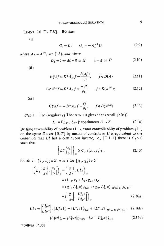
LEMMA 2.3. With reference to (2.36) we have for any E > 0 and for Ch3, = max[n/2, M,]:

Proof of Lemma 2.3. We estimate each term of (2.36) separately by Schwarz inequality (here below all norms are L2(Q)-norms):

T

Vq5.Vq5, dQ II G II Iv&n Iloll IV4,(T)l II + II IVd”l II II IV4’l II

G; i ; [II Ivd(nI 112+ II IVdOl II21 +cCII Iv4,(nl 112+ II IV&l II21 I

d f II IVG4 II $0. T,:Lqn)) +; [II Ivd,(nl 112+ II Iv4’ll121. (2.39)


Similarly, with 2M, E maxa 1 h 1:

IC(Q,> h ~v4m2l~l

G 244, { Ild,(UI II IV(4YT))l II + lld’ll II IWdO)l II i

+&M/ill IvMnI /12+ II Iv~~“l 11’1. (2.40)

Hence, using (2.36), (2.39), (2.40) we obtain with C,,,=max[n/2, M,]:

+C,,/mV4t(nI 112+ II IV(MT))l II2

+ II IV@ 112+ II IV(&“)l II’1 (2.41)

and (2.38) follows from (2.41) by use of the conservation of energy (2.37b). Lemma 2.3 is proved. 1

Step(v). Using (2.38) and (2.37b) in (2.38) we obtain for the right hand side of (2.29):

RHS of (2.29) > j”’ E(t) dr - 2&,$(O) 0

-2 Cn,h - [II IV41 /I&0,T,:&2)) + Il~rllZC(~O.T,:L~~R))l

= [T- ic,,,, E(O)

-2Cn,h y--- [II IV41 II&,.~,:~2wq~ + II~~II~,Eo,~,;~2~~~~I. (2.42)

Combining (2.32) with (2.42) we finally arrive at

Con%h,n [II IV& IIzCc~o,TI~L~~Q~~+ II Il~111ZC~~0.~3~~~~n~~l

++jx((y)‘+(g2) dC a [T- ~EC,,J E(0). (2.43)


Step (vi). To complete the proof of Proposition 2.2, we need the following Lemma, of the type already used in [L.3], in [L.2], in [L-T.31, [ L-T.71, etc.

LEMMA 2.4. (i) Inequality (2.43) implies: for any T> 0, there is C, > 0 such that for all {do, 4’) ED(A~‘~) x D(A’j4) we haoe

(2.44a)

(ii) for any sequence T, 7 00 we have

lim inf C, = 0 so that sup CT E C < c/3. (2.44b) T

Proof of Lemma 2.4. Part (i). The proof is by contradiction. Let there exist a sequence (qS,(t)) of solutions to problem (2.lSa, c, d, e) and (2.28) over [0, T]:

~I:+L12q5,=0 in Q (2.45a)

cj,(O, .)=~;ED(A~‘~), #;(O, .)=&ED(A”~) in Q (2.45b)

4nIz-0 in Z (2.45~)

@,I.-0 in C (2.45d)

(d/dt = ‘), given explicitly by

d,(t) = C(t) 4: + s(t) 4; E C(CO, Tl; D(A3’4)) (2.46a)

4:,(t)= -AS(t)+;+C(t)&EC([O, T];D(A1’4)), (2.46b)

such that

jj~)‘+(~)‘d.&O, as n+co. (2.47b)

By the preceeding steps (i)-(vi), each solution d,(t) satisfies inequality (2.43) and thus we have

En (0) = J IVdf, I2 + IV(&~)l 2 dQl < Const, uniformly in n. (2.48 ) R


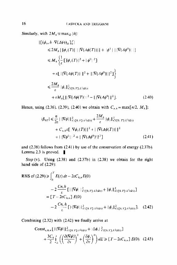
Recalling (1.7))( 1.8) HA = D(A’ ‘), we see that there is a subsequence, still subindexed by n, such that

4: --+ some function 4” in HA(Q) = D(A’,“) weakly (2.49a)

0: -+ some function 4 ’ in V = D( A “’ ) weakly. (2.49b)

We then consider the solution to problem (2.18a, c, d, e), (2.28) with initial data found in (2.49)

~(t)=C(t)~“+S(t)~‘EC([O, T],D(A3’4)) (2.50a)

(F(t) = -‘4S(t)(b0 + C(t)4 E C( [O, T]; D(P4)). (2.50b)

Then (see details, e.g., in [L-T.3, Sect. 21 in a similar situation corresponding to the wave equation), it follows that

4,(t) -+ m in L"(0, T, V=D(FI~‘~)) weak star (2.51a)

&f(t) + P(f) in L"(0, T; HA(R) = D(A’j4)) weak star. (2.51b)

Then (2.51) implies in turn that d,(t) and &(t) are uniformly bounded in L"(0, T; V) and L”(0, T; D(A”4)), respectively. This fact, along with the compactness of V -+ D(A1j4) = H;(Q) and of D(A’14) + L2(Q), implies [Sl, ‘Corollary 41 that there is a subsequence, still subindexed by n, such that

O,(~)+it(~) strongly in L"(0, T;HA(SZ)) (2.52)

&l(t) + &v) strongly in L'(0, T,L*(Q)). (2.53)

A fortiori, from (2.47a) and (2.52)-(2.53) we obtain

1 = II IVd,I Il&o.r,:L2,Q,) + IlKI II &[O.T,,L~w2))

-+ II IW II &o.T,:L’(n,, + II~‘II:r[o,r]:L’(n,, = 1. (2.54)

Moreover, by (2.47~)

Thus i(t) satisfies

&,+A2J=0 iI,

?.o ~0 av t ’

(2.56)


and, by differentiation in t, also

&,+L12$=o

f&=0, d&SO (2.57)

on [0, ZJ, with 0 < T-c cc arbitrary but fixed. Holmgren’s uniqueness theorem applied to (2.57) yields then T’ = 0 on Q, hence 7 E const in Q. By the boundary condition 4 1 Z = 0 in (2.56), we then conclude that 6 s 0 in Q, a contradiction with (2.54). The proof of Part(i) of Lemma 2.4 is complete.

Proof of pavt (ii). For each {do, 4’) E D(A314) x D(ALi4) = F and each T> 0 we set for convenience

Then we can take C, in (2.44) as defined by

(2.59)

(2.60)

which is finite by Part (i) for each 0 < T < co. Now, by contradiction, let there be a sequence T,,, T 00 such that

C, > p > 0 for all m. Since C, is finite for each m, definition (2.60) implies that: for each m large enough, there is a pair (4:. dk} E F of initial data such that

(2.61)

By normalization if necessary, we may achieve that such {d:, 4;) gives rise to

and hence, by (2.61) also to

< const, for all m. (2.63)

But the solution 4(t, d:, 4:) was shown earlier to satisfy inequality (2.43).


Thus by (2.62))(2.63) used in (2.43) we obtain (with I:’ = ~cc,,,,):

CT,,, - E’] E,,, (0) 6 const, uniformly in 1)~ (2.64)

E,(O)=j IV&‘+IV(dq5;)J’rlsz, (by (2.37b)). (2.65) R

Then (2.64) implies E, (0) 10, i.e., by (2.65) and ( 1.7b)-( 1.8b)

((& 4;) -+ 640) in D(A3”) x D(F!“~). (2.66)

It then plainly follows from (2.66) that the solution

satisfies

#(t, 4:, 4;) -+ zero function, in C( [O, co]; D(A”4)) (2.68)

#,(t, d”,, fjt) + zero function, in C( [O, ~01; L’(Q)) (2.69)

since IIC(t)ll, IIA “2S(t)ll < const, for all t E R in the uniform norm of L’(Q). But then (2.68)-(2.69) imply lim, NT,(dL, 0;) = 0, and this contradicts lim, Nr,,,(di, 0:) E 1 which follows from (2.62). Lemma 2.4 is fully proved. 1

Step (vii). We use Lemma 2.4 in (2.43) and obtain

COROLLARY 2.5. For any T> 0 and E sufficiently small we have the inequality

Consth,,~z(~)2+(~)‘dZ>[T-2eCi,~] E(O), (2.70a)

with (see 2.37b)):

E(O)= jD [Vq5’12 + IV(zt#“)12 dQ equivalent to II {do, ~‘}llf,~A~,~~XD,A~r~, (2.70b)

by (1.7) (1.8). Then, inequality (2.70a) a fortiori implies inequality (2.21)for T > 0 arbitrarily small. The proof of Proposition 2.2 is now complete.

Remark 2.1. At no extra effort over the proof of Lemma 2.4, we may


strengthen its statement to read: inequality (2.43) implies that for any T> 0 there is C,>O such that all {b”, 4’) ED(A~‘~) x D(A’j4) we have

(2.71)

Thus, a fortiori (2.71) implies that the characterization (2.21) in Lem- ma 2.l(iii) for exact controllability in the present section is equitdent to inequality (2.28) in Proposition 2.2.

3. PROOF OF THEOREM 1.2: EXACT CONTROLLABILITY ON q)(Q) x H-'(Q) ED(A"4) x [D(A"4)]'

We parallel and complement the proof of Theorem 1.1, by working this time on different spaces.

Step 1. We return to the input-solution operator L, = CL,,, LZT] in (2.1) and compute its adjoint L,” for Z= [or, ~~1 ED(A”~) x [D(A1’4)]’

(3.la)

(3.lb)

as in (2.16a), so that

II~,#,-II~~,o.r:~~~~~,xL*(z) = lIG%f~(o,r:L2(r)) + llG%ll2~,~, (3.2)

as in (2.16~). The (regularity) Theorem 1.0 gives

L,= CL,,, L,,]: continuous HA(O, T; L*(r))

x L*(z) + D(A”4) x [D(A’q]’ (3.3)

and exact controllability of problem (1.1) in the present section means that the above map in (3.3) is onto, or equivalently that: there is C,> 0 such that

II 2

(3.44 H~(0,r:L.‘lFl)xL21Z)

22 LASIECKA AND TRIGGrANI

or recalling (3.2)

where we have used that the HA(O, T)-norm is equivalent to the “gradient norm.”

Step 2. An equivalent partial differential equation characterization of inequality (3.4b) is given by the following lemma.

LEMMA 3.1. For ZE D(A’14) x [D(A’14)]’ we have:

(i)

(L,#,z)(t)=G:[C(t-T)A “2z2+S(t-T)(-A”‘z,)]

K,t+K&z;(O, T;L’(T)) (3Sa)

K,=K,,=T {[c(T)-I] AP”2z2+S(T)A”‘z,} (3Sb)

Kz=K?T=-G:[C(T)A~‘/Z=2+S(T)A’i’=,J

d(L%) 8(4&t)) + K -= -~ dr iJv IT?

(3.k)

(3.6)

where d(t) = d(t, q5’, 4’) is the solution of the following homogeneous problem, backward in time

qStr+A2qh=0 (3.7a)

OI,=T=~O~~,I,=T=~’ (3.7b)

fjlL=o (3.7c)

Aq5[,-0 (3.7d)

with

explicitly given by

$rqr)=c(t-T)qi”+S(t-T)~’ (3.8a)

~,(t)=AS(t-T)q,4°+C(t-Z-)#‘. (3.8b)


(ii)

(L2#,=)(r) =; dt(t), (3.9)

where d(t) solves (3.7).

(iii) For any 0 < T< co, inequality (3.4b) [which characterizes exact controllability ofproblem (1.1) on the space D(A’j4) x [D(A”4)]’ by means ofcontrols [g,, g,] E HA(O, T; L’(r)) x L*(X) over [0, T]] is equiualenf to:

there is C> > 0 such that

a(4) -Fr+K,~ ]2dZ+jz($) dC 2 c;. II {do, 6’ > II &43’4, x D(,4’.4,

(3.10a)

(3.10b)

Moreover, the map T + CT is monotone increasing.

Proof of Lemma 3.1. (i) With g, E HA(O, T; L’(T)), on the one hand we have

since g, vanishes at t =0 and t = T; on the other hand, using (2.2) we readily compute as usual (Lemma 2.1)

tL,Tg,, z, D(,4’,4) Y [0(,4’?4)]’ = S(T-t)G, g,(t)dt, A3”z1 > LW I

~oTC(T-t)G,g,(l)dt,A1~2z, > Lw? )

= o’(g,(t),G:[S(T-t)A3’2z, I

+ C( T- t) A “*z~])~>~~, dt (3.12)


SO that comparing (3.11) with (3.12) and using that C( . ) is even while S( ) is odd

-~(L~T~)=G~~C(r-T)A’,‘;,+S(,-T)(-AJ;’.-,),. (3.13)

Integrating in t we readily find

~(L:,z)(r)=-G:[s(r-T)A”‘;,A~‘C(i-T)(-A””~,)]+K,

(3.14)

(L,#,z)(~)=G:[A-‘S(~-T)(-A~‘~Z,)

+A~‘C(t-T)A1’2z2]+K,t+K2. (3.15)

By imposing that (L1#,z)(t) vanishes at t = 0 and t = T, so that L,#,ZE HA(O, T; L’(T)), we readily identify the operators K, and K, as in (3Sa-b), and (3.15) then becomes (3Sa). For the purposes of (3.4b) we now re-write (3.14) as

d(LrT=Nt) dt

= -G:AIC(t-T)A~“‘zl+S(t-T)A~‘i’-,]+K,,

= ~WW)) + K

av IT9 (3.16)

where in the last step we have used (2.11) and (3.8a).

(ii) With g, E L’(C) we compute from (2.3) as before

(L,g,, Z)D(.41,4,x [D(/f’J)],

(1 T

= S(T-t)G2g2(t)dt,A3”z, 0 > L+R)

G, g, (t ) dt, A “‘z, > L+2)

= s oT (g2(t), G: [S(T-t) A3’2z1 + C( T- t) A1’2z2])Lz,r, dt

= (g,? ‘fTz)Lz,Z,. (3.17)

Thus

(L&z)(t)=G~[C(t-T)A”2z2+S(r-T)(-/43’2z1)]

ad,(t) =G:A[C(r-T)A~“‘--2-AS(t-T)A~~‘~2~,]=I:Y, (3.18)


where in the last step we have used (2.13) and (3.8b), (3.7~). Part (ii) is proved. As to Part (iii), we first note that by (3.7e)

II(z-] =A1’2cjo, z2=A”2$is1}1/ D(/‘l.J)X [D(A1/4)]‘= II {A3’440, A”441 III L2(R)X L.*(n)

= II{d”, ~1)IID,A3i4)xD(AI~4,. (3.19)

Moreover, from (3.5b) and (3.7e)

KlT=~{[C(T)-z]A-“2z2+AS(T)A-“2zl}

=?{[C(T)-z]g’+As(T)m”).

Then, (3.4b) becomes (3.10a-b) as desired, by use of (3.6), (3.20), (3.9), and (3.19). The proof that T + C> is monotone increasing is conceptually the same as the one given for inequality (2.21), just below (2.28). The proof of Lemma 3.1 is complete. 1

Step 3. We “absorb” the lower order term K,,, the boundary vector given by (3.10b), in the lefthand side of inequality (3.10a), through an argument of the same type as the one in Lemma 2.4.

LEMMA 3.2. Inequality (3.1Oa)-which characterizes exact controllability ouer [0, T] on the space G?,(FI”~) x [LS(A”~)]’ by means of controls [g,, g2] E Hh(O, T; L2(ZJ) x L’(C)-is equivalent to inequality (1.26) = (2.28a)-which characterizes exact controllability over [0, T] on the space [~(LI”~)]’ x [9(1!~‘~)]’ by means of controls [g,, g,] E L,(C) x [H’(O, r; L2(z-))I’.

Proof We assume inequality (3.10a) and we wish to show that, in fact, there exists a constant C,>O such that

(3.21)

so that inequality (1.26) = (2.28a) will likewise hold true. Suppose by contradiction that there exists a sequence {4,,(t)} of solutions to problem

(1.24)

d;+A2d,=0 in Q

441r=O=4nO~~(~3’4), 4:,It=o=4nl~~w’4) in52 (3.22)

4nlr=4,Ir-0 in C


such that

(3.23)

as ‘I--+ xl (3.24)

By assumption, all the {d,(t)> satisfy inequality (3.10a) and so by (3.23) there is a subsequence {don, S,,} converging to some {&, 4, } weakly in g(A3’4) x g(A 1’4) and hence, by compactness of A ‘, strongly in WA 3’4-6)~9(A’!4pd) for 6~0. As a consequence, we return to (3.10b) and see that

converges strongly in L*(r) to (3.25)

a,,=? ([C(T)-I] 4, +AS(T)$,}

since G: is a bounded operator L’(Q) -+ L*( ZJ. Using (3.23), (3.24), (3.25 we conclude that

lImL~(~)= 1 (3.26

On the other hand, q(t) = C( t)$, + S(t)$, satisfies

&,+A2J=0 in Q

)

)

&=A~,=0 in C (3.27)

= 0 from (3.24)) in Z

for 0 < t Q T. After differentiating (3.27) in t, we apply Holmgren uniqueness Theorem CH.2, p. 1291 and conclude that p = 0 in Q, hence $ = 0 in Q by (3.27b), i.e., $, = $, = 0. Finally, by (3.25) we obtain R,,= 0. But this contradicts (3.26).

The proof that inequality (1.26) = (2.28a) implies inequality (3.10a) is identical. a

Proof of Corollary 1.3. (i) This part is proved in Lemma 3.2. By Remark 2.1, inequalities (2.21) and (2.28) are equivalent. By Lemma 3.2, inequalities (2.28) and (3.10) are equivalent.


(ii) We apply th e interpolation Theorem [L-M.l, Theorem 5.1, p. 271 to the operator LFpl which, by part (i) is bounded between the space in (1.32) and the space in (1.30) at the end points 8 = 0 and 0 = 1. Hence, LFp ’ is continuous between the interpolation spaces

[D(A”4) x [D(lP4)]‘, [D(FP4)] x [D(A3’4)]‘],

and the interpolation spaces

[H:,(O, T; L’(r) x L’(C), L?(C) x [H’(O, T; L’(l-))I’&

0 < f3 < 1, which means that L, is onto in the opposite direction. Then (IL-M.l, p. 64-661 gives (1.30) while [L-M.l, p. 29) gives (1.31). 1

APPENDIX A: PROOF OF IDENTITY (2.1)

Let h(x) E C*(o). With reference to Remark 1.2, we multiply Eq. (2.20a) by h .V(d#) and integrate over Q. We shall use the identity

1 D

h.VqdQ=j qh.vdr-1 qdivhdQ (A.11 I- a

obtained from div(qh) = h . Vq + q div h, q scalar function, and the divergence theorem. In addition, we shall use the identity

j Q

@(h+)dQ=j ~(h.VI)d~-~jl,V~,*h.“dZ z

-J’ HVII,.V$dQ+iJQlV$j2divhdQ (A.2) Q

already proved in, say, CT.3, Eq. (A.3) of Appendix A] (with similar multiplier techniques) where H= H(x) is the transpose of the Jacobian matrix of h(x):

ah, ah,

H(x) = i3.u,’ . ..’ ax,

ah, ah” (A.31

-’ . ..’ ax, ax,

Term 4,,h . V(+). Integrating at first by parts in t

j j’q&,h.V(d))dfdQ=[j qi,h-V(Aq4)dl2]‘-j 4th .V4,) dQ R 0 P 0 Q


[using (A.1) with h there replaced by ~$,h now. with q = AqS, and with

div(d,h) = Vd,. h + 4, div h]

4, Aq5,h. v d/T

+ j A#,y3, div h dQ. (A.41 Q

A#,h .Vd, dQ + j Q

[Using identity (A.2) with tj=q4, for the third integral on the right of (A.419

j I’q$,h.V(AqUdtdlJ=[j q3,h-V(Aq5)df2]T- j 4, AqS,h . v dC D 0 R 0 z

-; jz IV#,)‘h.vd.Z+ jz~h.V&dZ

- 1 HV(,.Vd,dQ+kj IV#,l’divhdQ P Q

+ j Aqb,qS,divhdQ. (A.51 Q

Using Green’s first theorem on the last integral at the right of (A.5) along with the identity

V#, .V(d, div h) = 4, V(div h) .V&, + IVb,]’ div h

we finally obtain from (A.5)

I d,,h .VA4) dQ Q

:j IVq512h.rdL’+jx~h.V#,dZ+jx~~,divhdZ. --

r

-j HV),.V(,dQ-ij IV4,12divhdQ Q Q

- s

4, V(div h) .V#, dQ. Q

(f4.6)


Term A’$h . V( A$). Using identity (A.2) this time with $ = Ad we obtain

s A(A#)h .V(Ad) dQ Q

= s r

~h.V(A+L+” IV(Aq5)12h.vdZ 5

-s HV(A41.V(A#)dQ+kjQ IV(Aq5)j’divhdQ. (A.7 1 Q

Summing up (A.6) and (A.7) and recalling (1.2a) we finally obtain

s a(@) zlh.V(A()d.Z+[z$h.V~,dZ+~ zq5,divhdZ

z

-~~=lV~,12h.vd=-~~=IV(Ag)lzh.vdL.-?: 4, Ad,h. v dC z

+ij {I~~,l’-I~(~~)l’~divhdQ Q

+ s Q 4, V(div h) .Vd, dQ

- C(d,, h.v(A~)),l,‘+~Qfll.V(A~)dQ (A.8 1

which is the sought after identity for 4 satisfying (1.2a).

Specialization of Left Hand Side of (A.8) to 4 which Satisfies also the Boundary Conditions (2.20~4). Recalling (2.20~4) we have

d,lz-OO;Vq4 -L rand IVq4( = on C by (2.20d) (a)

(A.9) ad, -&-

=O;Vq5,If and IVq+,l= $$ =O I I

in Z. (b)

409 146 I-?


Thus, using (2.20cd) and (A.9a-b) in the left hand side (LHS find that this simplifies to

) of (A.8 ) we

LHS of (A.8) = ?*, y wAqw-~j IV(Aq5))‘h.v L-

d‘. (A.10)

Specialization of the Right Hand side of (A.8) to Radial Vector Fields II =.Y-.x0. In this case, recalling (A.3) we obtain

H( .u) = identity matrix; div /Z = n = dim Sz (A.1 1)

which used in the right hand side (RHS) of (A.8) yield

RHS of (A.8) = i‘ :IW,l’+ IV(4h121 dQ Q

x s .fh .V(@) dQ- [Cd,> h ~WW,l;. (A.12) Q

Combining (A.lO) and (A.12) proves (2.1), as desired.

APPENDIX B: PROOF OF IDENTITY (2.34)

Again, we shall first obtain an identity, (B.3) below, for 4 which solves only (2.18a) and for arbitrary smooth vector field h E C’(0). Next we shall specialize this identity (B.3) to the case where 4 satisfies in addition also the boundary conditions (2.18c-d) and, moreover, the vector field is radial.

We multiply Eq. (2.18a) by d4 div h and integrate over Q by parts in t and by Green’s first theorem:

ss 7‘ q5,, A4 div hdtdL? R 0

= [?’ T T

Aq5 I$, div h dl2 R 1 jj - Aq5,q5, div h ds2 dt

0 0 R

=Lr rg4,divhdTj Vd.V(m,divh)dn]T

R 0

-s z !$d, div h dC + j IV4,1Z div h dQ + $ #,V(div h) . V4, dQ Q Q

(B.1)

also

EULER-BERNOULLI EQUATION

r

ss A(Aq5) Aq5 div h dQ dt

0 R

31

= I acAd) -AddivhdZ z av

- /Q lV(A()/2divhdQ-jQA#V(divh).V(A()dQ. (B.2)

Summing up (B.l) and (B.2) we find the identity

I (IV4,12- IV(A4)12) divhdQ Q

+ [ Aq5 V(div h) .V(Atj) dQ - [ d,V(div h) .V$, dQ JR JQ

IQ A#.V(@,divh)dQ- 3 I r av

for q5 satisfying (2.18a). If now h(x) is a radial vector field, then (see

(2.34).

1 7

i, div h dT (B.3) 0

2.33)), (B.3) specializes to

REFERENCES

IF-L-T.11 F. FLANDOLI, I. LASIECKA, AND R. TRICGIANI, Algebraic Riccati equations with nonsmoothing observation arising in hyperbolic and Euler-Bernoulli equations, Ann. Mat. Pura Appl. (4) 153 (1988), 307-382.

LG.11 P. GRISVARD, A Caractbrization de quelques espaces d’interpolation, Arch. Rational Mech. Anal. 25 (1967), 4&63.

CH.11 L. F. HO, Observabilitt de frontiere de l’tquation des ondes, C. R. Acud. Sci. Paris Sk. I Math. 302 (1986).

CK.11 V. KOMORNIK, Controlabiliti exacte en un temps minimal, C. R. Acad. Sci. Paris Shr. I Math. 304, No. 3 (1987).

https://www.researchgate.net/publication/284693127_Controlabilite_exacte_en_un_temps_minimal?el=1_x_8&enrichId=rgreq-2e22ddc3-5a58-40df-80e5-41c6af9c638b&enrichSource=Y292ZXJQYWdlOzI0MjY1NTg1NztBUzoxMTQwODkwOTUzNDAwMzNAMTQwNDIxMjM2ODczMg==



https://www.researchgate.net/publication/225861667_Algebraic_Riccati_equations_with_non-smoothing_observation_arising_in_hyperbolic_and_Euler-Bernoulli_boundary_control_problems?el=1_x_8&enrichId=rgreq-2e22ddc3-5a58-40df-80e5-41c6af9c638b&enrichSource=Y292ZXJQYWdlOzI0MjY1NTg1NztBUzoxMTQwODkwOTUzNDAwMzNAMTQwNDIxMjM2ODczMg==

https://www.researchgate.net/publication/225861667_Algebraic_Riccati_equations_with_non-smoothing_observation_arising_in_hyperbolic_and_Euler-Bernoulli_boundary_control_problems?el=1_x_8&enrichId=rgreq-2e22ddc3-5a58-40df-80e5-41c6af9c638b&enrichSource=Y292ZXJQYWdlOzI0MjY1NTg1NztBUzoxMTQwODkwOTUzNDAwMzNAMTQwNDIxMjM2ODczMg==


IL.11 J. L. LIONS, “Controle des systems distribues singuliers.” Gauthier-Villars. Paris. 1983.

IL.21 J. L. LIONS, “Exact Controllability, Stabilization and Perturbations, SIAM Ret&v 30 (1988). 1-68. To appear by Masson in extended form.

LL.31 W. LITTMAN. Near optimal time boundary controllability for a class of hyperbolic equations. in “Lecture Notes in Control and Information Sciences,” Vol. 97. pp. 307-312. Springer-Verlag. New York, 1987.

LL.41 W. LITTMAN. “Boundary Control Theory for Beams and Plates, CDC Conference, Fort Lauderdale, 1985.” Vol. III, pp. 2007-2009.

CL.51 J. LAGNESE. Decay of solutions of wave equations in a bounded region with boundary dissipation, J. Dijjferenfial Equations 50 (1983), 163-182.

D-61 I. LASIECKA, Controllability of a viscoelastic Kirchhoff plate. Birkhluser 1989, International Series of Numerical Mathematics No. 91, pp. 237-247.

IL-L.11 J. LAGNESE AND J. L. LIONS. Modelling, analysis and control of thin plates. Masson 1988.

CL-M.11 J. L. LIONS AND E. MEGENES. “Non-homogeneous Boundary Value Problems and Applications,” Vols. I, II, Springer-Verlag. New York, 1972.

CL-L-T.11 I. LASIECKA. J. L. LIONS. AND R. TRIGGIANI. Non-homogeneous boundary value

[L-T.11

CL-T.21

IL-T.31

[ L-T.41

CL-T.51

CL-T.61

[ L-T.71

[L-T.81

cs.11

CT.11

CT.21

problems for second order hyperbolic operators, J. Math. Pures Appl. 65 ( 1986). 149-192. I. LA~~ECKA AND R. TRIGCIANI, Uniform experimental energy decay of the wave equation in a bounded region with LZ(O, co: L?(T)bfeedback control in the Dirichlet boundary conditions, Differential Equafions 66 (1987), 34g-390. I. LASIECKA AND R. TRIGGIANI, A cosine operator approach to modeling LZ(O, r; L,(T)tboundary input hyperbolic equations, Appl. Muth. Optim. 7 ( 1981). 35-83. I. LA~~ECKA AND R. TRIGGIANI, Exact controllability for the wave equation with Neumann boundary control, Appl. Math. Opfim. 19 (1989). 243-290. I. LASIECKA AND R. TRIGGIANI, Regularity of hyperbolic equations under Lz(O. T; Lz(T))-boundary terms, Appl. Marh. Opfim. 10 (1983). 275-286. I. LASIECKA AND R. TRIGGIANI, Riccati equations for hyperbolic partial differential equations with Lz (0, T; L?(T))-Dirichlet boundary terms, SZAM J. Control Optim. 24 (1986), 884-926. I. LASIECKA AND R. TRIGGIANI, Exact controllability of the Euler-Bernoulli equation with L,(C)--control only in the Dirichlet boundary conditions, Atfi Accad. Naz. Lincei Rend. Cl. Sci. Fis. Mat. Natur. Vol. LXXXII, No. 1. (1988) Rome. I. LASIECKA AND R. TRIGGIANI, Exact controllability of the Euler-Bernoulli equations with controls in the Dirichlet and Neumann B. C.: a non-conservative case, SIAM J. Control Opfim. 27 (1989), 330-373. I. LASIECKA AND R. TRIGGIANI, Regularity theory for a class of Euler-Bernoulli equations: a cosine operator approach. Boll. Un. Mat. Ital. (7). 3-B (1989). 199-228. J. SIMON, Compact sets in the space Lp(O, r B), Annali di Mafemafica Pura e Applicafa (Ib’), Vol. CXLVI. ( 1987), 65-96. R. TRIGGIANI, A cosine operator approach to modeling Lz(O, T; L,(T)j- boundary input problems for hyperbolic systems, in “Lecture Notes in Control and Information Sciences, Springer-Verlag. New York, 1978, pp. 38s-390; Proceedings 8th IFIP Conference, University of Wiirzburg, W. Germany, 1977. R. TRIGGIANI, Exact boundary controllability on L*(Q) x H-‘(O) for the wave equation with Dirichlet control acting on a portion of the boundary, and related problems, Appl. Math. Optim. 18 (1988). 241-277.


CT.31 R. TRIGGIANI, Wave equation on a bounded domain with boundary dissipation: an operator approach, J. Mafh. Anal. Appl. 137 (1989), 438461.

[T-L. 11 A. TAYLOR AND D. LAY, “Introduction to Functional Analysis,” 2nd ed., Wiley, New York, 1978.

IZ.ll E. ZUAZUA, Exact controllability of distributed systems for arbitrarily small time, C.R. Acad. Sci. Paris SPr. I Math. 804 (1987), 173-176.

https://www.researchgate.net/publication/234781508_Introduction_to_Functional_Analysis?el=1_x_8&enrichId=rgreq-2e22ddc3-5a58-40df-80e5-41c6af9c638b&enrichSource=Y292ZXJQYWdlOzI0MjY1NTg1NztBUzoxMTQwODkwOTUzNDAwMzNAMTQwNDIxMjM2ODczMg==

https://www.researchgate.net/publication/234781508_Introduction_to_Functional_Analysis?el=1_x_8&enrichId=rgreq-2e22ddc3-5a58-40df-80e5-41c6af9c638b&enrichSource=Y292ZXJQYWdlOzI0MjY1NTg1NztBUzoxMTQwODkwOTUzNDAwMzNAMTQwNDIxMjM2ODczMg==

https://www.researchgate.net/publication/243009904_Wave_equation_on_a_bounded_domain_with_boundary_dissipation_An_operator_approach?el=1_x_8&enrichId=rgreq-2e22ddc3-5a58-40df-80e5-41c6af9c638b&enrichSource=Y292ZXJQYWdlOzI0MjY1NTg1NztBUzoxMTQwODkwOTUzNDAwMzNAMTQwNDIxMjM2ODczMg==



Exact Controllability of the Euler-Bernoulli Equation with L2 (Σ)-control Only in the Dirichlet Boundary Conditions

Documents