Evolving scheduling rules with gene expression programming for dynamic single-machine scheduling problems

ORIGINAL ARTICLE

Evolving scheduling rules with gene expression programmingfor dynamic single-machine scheduling problems

Li Nie & Xinyu Shao & Liang Gao & Weidong Li

Received: 9 July 2009 /Accepted: 4 January 2010# Springer-Verlag London Limited 2010

Abstract The paper considers the problems of schedulingn jobs that are released over time on a machine in order tooptimize one or more objectives. The problems are dynamicsingle-machine scheduling problems (DSMSPs) with jobrelease dates and needed to be solved urgently because theyexist widely in practical production environment. Geneexpression programming-based scheduling rules construc-tor (GEPSRC) was proposed to construct effective sched-uling rules (SRs) for DSMSPs with job release datesautomatically. In GEPSRC, Gene Expression Programming(GEP) worked as a heuristic search to search the space ofSRs. Many experiments were conducted, and comparisonswere made between GEPSRC and some previous methods.The results showed that GEPSRC achieved significantimprovement.

Keywords Single machine scheduling . Dynamicscheduling . Release dates . Scheduling rules . Geneexpression programming

1 Introduction

Scheduling plays an important role in a shop floor controlsystem, which has a significant impact on the performance

of the shop floor. Scheduling is to allocate scarce resources(usually are machines) to activities (usually are jobs) withthe objective of optimizing one or more performancecriteria (for instance, minimizing makespan, flow time,lateness, or tardiness) [1]. In recent years, more and moreeffective scheduling methods for shop floor control haveemerged with the developments in scheduling methodolo-gies (in research and in practice) as well as technologicaladvances in computing.

Scheduling problems investigated by researchers forseveral decades may be categorized roughly into two types,static scheduling problems and dynamic scheduling prob-lems. In static scheduling problems, it is usually assumedthat the attributes of all jobs to be scheduled are availablesimultaneously at the start of the planning horizon andunchanged during the planning horizon. The assumption ismade mainly for the sake of convenience to model thesystem considered and solve the scheduling problems thatexist. However, the assumption does not always accordwith the practical production environment, since there arealways all kinds of random and unpredictable events thatoccur. For example, jobs arrive continuously over time,machines break down and are repaired, and the due dates ofjobs are changed during processing. It is rarely possible thatthe attributes of all jobs to be scheduled are available at thestart of planning horizon and unchanged during the horizon.Most scheduling problems that exist in such environmentare called dynamic scheduling problems [2]. Dynamicscheduling problems have attracted more and more atten-tion. For example, Kianfar et al. [3] studied a flexible flowshop system considering dynamic arrival of jobs; Wang etal. [4] considered the single-machine scheduling problemwith a deteriorating function, which means that the actualjob processing time is a function of jobs already processed;Ham and Fowler [5] considered the scheduling of batching

L. Nie :X. Shao : L. Gao (*)The State Key Laboratory of DigitalManufacturing Equipment and Technology,Huazhong University of Science and Technology,Wuhan, Hubei 430074, People’s Republic of Chinae-mail: [email protected]

W. LiFaculty of Engineering and Computing, Coventry University,Coventry, UK

Int J Adv Manuf TechnolDOI 10.1007/s00170-010-2518-5

operations with job release dates in wafer fabricationfacilities. Although some of static scheduling problemsare often solvable exactly in polynomial time, most of themare NP-hard. Dynamic scheduling problems are usuallymore difficult to solve than static ones.

The paper considers the problems of scheduling n jobsthat are released over time on a machine in order tooptimize one or more objectives, which are dynamic single-machine scheduling problems (DSMSPs) with job releasedates. The problems are considered for the followingreasons: First, dynamic scheduling problems exist widelyin practice and need to be solved urgently, although theypose bigger challenges than static scheduling problems.Secondly, single-machine scheduling problems often formcomponents of solutions for more complex schedulingenvironments. For example, a job shop scheduling problemmay be decomposed into single-machine sub-problems [6].

Static scheduling problems have been studied for almosthalf of a century, and many effective methods have beenproposed. At the beginning, many enumerative-basedtechniques have been developed. Although enumerativemethods such as branch and bound usually provide optimalsolutions, the cost of computation time is huge even for amoderate size problem [7]. In the last decades, therefore,many heuristic methods, including dispatching rules [8] andsearch-based methods, such as simulated annealing [9],tabu search [10], and genetic algorithms (GAs) [11] havebeen developed to solve larger problems in a reasonabletime. Search-based methods usually offer high-qualitysolutions. However, neither enumerative-based techniquesnor search-based methods are appropriate in dynamicconditions, because once the schedule is prepared, theprocessing sequence of all jobs is determined, and it isinevitable to modify the schedule frequently to respond tothe change of the system.

Over the last two decades, much effort has been made topropose new strategies or approaches to solve dynamicscheduling problems. Aytug et al. [12] categorized roughlyexisting strategies into three classes: completely reactiveapproaches, robust scheduling approaches, and predictive–reactive approaches. Completely reactive approaches havebeen widely employed in a large number of schedulingsystems and formed the backbone of much industrialscheduling practice. The approaches are characterized byleast commitment strategies such as real-time dispatchingthat create partial schedules according to the current state ofthe shop floor and the production objectives. Manyheuristics, also called dispatching rules, are frequently usedto examine the jobs waiting in processing at the givenmachine or those that arrive in the immediate future, at eachtime t when the machine is idle and to compute a priorityvalue for each job. The next job to be processed is selectedfrom them by sorting and filtering them according to the

priority values assigned to them and selecting the job at thehead of the resulting list. The priority function which isencapsulated in the heuristic and assigns values to jobs isusually called with the term scheduling rules (SRs) [1].

Several important achievements on DSMSPs with jobrelease dates are reviewed below. An online algorithm tominimize makespan problem, now commonly called listscheduling, was firstly investigated by Graham [13]. It is asimple greedy algorithm and does not use the informationabout processing times of jobs. Similar to the work ofGraham, other researchers made other research on theonline heuristics and achieved many results. As for the totalcompletion time problem, if all jobs are released at thesame time, Smith showed that the problem can be solvedoptimally by the well-known shortest processing time(SPT) rule [14]. For the preemptive version, Baker’s workshowed that it is easy to construct an optimal scheduleonline by always running the job with shortest remainingprocessing time (SRPT) [15]. In the case of single-machinenon-preemptive scheduling for minimizing the total com-pletion time, Hoogeveen and Vestjens [16] gave online 2-approximation algorithms, called delayed SPT rule, andproved that the lower bound on online scheduling is 2.Phillips et al. [17] gave a different 2-competitive algorithmcalled PSW algorithm, which converts preemptive sched-ules to non-preemptive schedules while only increasing thetotal completion time by a small constant factor. It isnoticeable that it was not the average flow time of a set ofjobs that was studied in the literature. Although averageflow time is equivalent to average completion time atoptimality, Kellerer et al. [18] have shown that theapproximability of these two criteria can be quite different.Guo et al. [19] modified the PSW algorithm to solveminimizing total flow time on a single machine with jobrelease dates and proved that this new algorithm yieldsgood solutions for the problem on average. Other objectivefunctions were rarely considered under the model of thedynamic single-machine scheduling with job release dates.For a review on online scheduling results, the comprehen-sive reviews of [20, 21] are referred. Apart from thesesimple online heuristics, other classical scheduling ruleswere also reported in literatures, which are the results ofdecades of research [22].

The general conclusion on scheduling rules is that norule performs consistently better than all other rules under avariety of shop configurations, operating conditions, andperformance objectives, because the rules have all beendeveloped to address a specific class of system config-urations relative to a particular set of performance criterionand generally do not perform well in another environmentor for other criteria. Therefore, many researchers madeeffort to exploit several methods based on artificialintelligence to learn to select rules dynamically according

Int J Adv Manuf Technol

to the change of the system’s state from a number ofcandidates. For example, Jeong and Kim [23] and Yin andRau [24] used simulation approach; Chen and Yih [25] andEl-Bouri and Shah [26] used neural network; Aytug et al.[27] used genetic learning approach; Trappey et al. [28]used expert systems; Singh et al. [29] used the approach ofidentifying the worst performing criterion; and Yang andYan [30] used adaptive approach. These methods aremainly based on learning to select a given rule from amonga number of candidates rather than identifying new andpotentially more effective rules. However, significantbreakthrough beyond current applications of artificialintelligence to production scheduling have been made byother researchers who made it possible to automaticallyconstruct effective rules for a given scheduling environ-ments. One of the typical works was the learning systemSCRUPLES proposed by Geiger et al. [31]. The systemcombined an evolutionary learning mechanism, i.e., Genet-ic Programming (GP) [32], with a simulation model of theindustrial facility under study, which automates the tediousprocess of developing new scheduling rules for a givenenvironment which involves implementing different rulesin a simulation model of the facility under study andevaluates the rules through extensive simulation experi-ments. Other existing similar researches include: Dimopoulosand Zalzala [33] evolved rules with GP for single-machinetardiness problem; Yin et al. [34] evolved rules with GP forsingle-machine scheduling subject to breakdowns; Jakobovicand Budin [1] evolved rules with GP for dynamic singlemachine and job shop problem; Atlan et al.[35] andMiyashita [36] applied GP mainly to classic job shoptardiness scheduling; and Tay and Ho [37-39] focused onevolving rules with GP for flexible job shop problem.The characteristic shared by these works is that it is thespace of algorithms but not that of potential schedulingsolutions is searched with an evolutionary learning mech-anism. The point in the space of potential schedulingsolutions presents only a solution to the specific schedulinginstance, which means that a new solution must be foundfor different initial conditions. While the point in the spaceof algorithms represents a solution for all of the problems,instances in a scheduling environment with an algorithmcan be used to generate a schedule [1]. However, these GP-based approaches mentioned above have a huge cost oncomputation time, and the constructed rules are usuallyformulized complexly.

In this research, gene expression programming-based SRconstructor (GEPSRC) was proposed to automaticallydiscover effective SRs for DSMSPs with job release dates.Gene Expression Programming (GEP), one of the evolu-tionary algorithms, worked as a heuristic search to searchthe space of algorithms but not that of potential schedulingsolutions. The proposed approach was evaluated in a

variety of single-machine environment where the jobsarrive over time. GEP was usually possible to discoverrules that are competitive with those evolved by GP and theclassical heuristics selected from literature. In addition, thecomputation requirement for training GEP to discover highperforming rules is much less than that of GP.

The remainder of the paper is organized as follows.Section 2 gives the statement of the DSMSPs with jobrelease dates. Section 3 describes the heuristic for thescheduling problems. Section 4 proposes the frameworkand mechanism of the GEPSRC and describes the applica-tion of GEPSRC on the scheduling problems. An extensivecomputational study is conducted within the single-machineenvironment to assess the efficiency and robustness of theautonomous SRs constructing approach. The experimentsand results are provided in Section 5. Section 6 is theconclusion and future work.

2 Statement of dynamic single-machine schedulingproblems

The DSMSPs with job release dates is described as follows.The shop floor consists of one machine and n jobs, whichare released over time and are processed once on themachine without preemption. Each job can be identifiedwith several attributes, such as processing time pi, releasedate ri, due date di, and weight wi, which denotes therelative importance of job i, i=1,…, n. The attributes of ajob are unknown in advance unless the job is currentlyavailable at the machine or arrive in the immediate future. Itis also assumed that the machine cannot process more thanone job simultaneously. The scheduling objective is todetermine a sequence of jobs on the machine in order tominimize one or more optimization criteria, in our case,makespan, total flow time, maximum lateness, and totaltardiness, respectively. For the sake of convenience, weassume all jobs relatively equal, i.e., wj=1. Then, the fourperformance criteria considered are defined below.

Cmax ¼ max ci; i ¼ 1; :::; nð Þ ð1Þ

F ¼Xni¼1

ci � rið Þ ð2Þ

Lmax ¼ max ci � di; i ¼ 1; :::; nð Þ ð3Þ

T ¼Xni¼1

max ci � di; 0ð Þ ð4Þ

Int J Adv Manuf Technol

where ci denotes the finishing time of job i. Cmax, F, Lmax,and T denote makespan, total flow time, maximum lateness,and total tardiness of a problem instance, respectively.

Since GEP is used to search the space of algorithms butnot that of potential scheduling solutions in the paper; thescheduling algorithms are evaluated on a large number oftraining sets or test sets of problem instances, whichrepresent different operating conditions relative to differentperformance criteria, respectively. In order for all thetraining sets or test sets to have a similar influence to theoverall performance estimation of an algorithm, averagecriterion value over the training set or test set of probleminstances are defined as below.

Cmaxj j ¼ 1

t

Xt

j¼1

Cmax;j

nj � pj¼ 1

t

Xt

j¼1

max cij; i ¼ 1; :::; nj� �

nj � pjð5Þ

Fj j ¼ 1

t

Xt

j¼1

Fj

nj � pj¼ 1

t

Xt

j¼1

Pnji¼1

cij � rij� �

nj � pjð6Þ

Lmaxj j ¼ 1t

Ptj¼1

Lmax;j

nj�pj ¼1t

Ptj¼1

max cij�dij;i¼1;:::;njð Þnj�pj ð7Þ

Tj j ¼ 1

t

Xt

j¼1

Tjnj � pj

¼ 1

t

Xt

j¼1

Pnji¼1

max cij � dij; 0� �

nj � pjð8Þ

where Cmax,j, Fj, Lmax,j, and Tj denote the makespan, totalflow time, maximum lateness, and total tardiness ofproblem instance j, respectively; nj denotes the number ofjob in problem instance j; pj denotes the mean processingtime of all jobs in problem instance j; cij, rij, and dij denotecompletion time, release date, and due date of job i inproblem instance j, respectively; t denotes the number ofinstances in a training set or test set; and |Cmax|, |F|, |Lmax|,and |T| represent the average value of makespan, flow time,maximum lateness, and tardiness over the training set ortest set of problem instances. It is obvious that algorithmswith less objective values of |Cmax|, |F|, |Lmax|, and |T| arebetter.

3 Heuristic for DSMSPs with job release dates

In static circumstance, since the attributes of all jobs to bescheduled are available at the beginning of planninghorizon (referred to be time 0) and unchanged during theplanning horizon, the whole schedules usually can be madeat the beginning. However, it is not convenient in dynamicconditions where jobs arrive over time and the release datescannot be known in advance. At any time, some jobs havearrived and others may arrive in some future moment. Inthis section, we describe a heuristic for the schedulingproblems on a single machine with job release dates, andthe release dates are unknown in advance unless the jobswill arrive in the immediate future. This heuristic wasproposed firstly by Jakobovic and Budin [1].

Heuristic for DSMSPs with job release dates: Initialize t = 0, where the machine is idle at time t;

While there are unscheduled jobs do

JSs(t) = {all jobs satisfied with wtj < Pmin(t) };

Calculate priority values for all the jobs in JSs(t) according to a SR;

Schedule the job with the best priority on the machine, and denote the job with J*;

Update the machine’s idle time, i.e. t = the completion time of J*;

End while.

Where JSs(t) represents the set of the jobs to be takeninto consideration for scheduling at time t; wtj denotes thewaiting time for the arrival of the job j, i.e., wtj=max{rj − t, 0};Pmin(t)denotes the shortest processing time of the jobs thatalready arrived but are unscheduled at time t.

It is obvious that the JSs(t) consists of two types of jobs:the jobs that already arrived but are unscheduled at time t

(denoted with AType) and those that are expected to arrivedsoon and satisfy wtj<Pmin(t) at time t (denoted with BType).It is the SR encapsulated in the heuristic that is responsiblefor evaluating the priority value for each AType job orBType job.

It is noticeable that the “best priority” may be defined asthe one with the greatest or the lowest value. In the paper,

Int J Adv Manuf Technol

we define that the job with a lower priority value has betterpriority.

The heuristic for DSMSPs with job release dates isemployed in the paper for the reasons as below. First, boththe arrived jobs (AType job) and the jobs that are expected toarrive soon (BType jobs) are taken into consideration forscheduling, which contributes to make a more reasonablescheduling decision. In practical scheduling environments, ajob can be identified if it arrives in the immediate future. Totake jobs that are expected to arrive in the immediate future(BType jobs) into consideration provides a more globalperspective for scheduling manager. Second, it dramaticallydecreases the computation cost for estimating priority valuesto exclude the jobs with wtj≥Pmin(t) from the set of JSs(t).For any regular scheduling criterion, such as minimizingmakespan, flow time, maximum lateness, and tardiness, thejobs with wtj≥Pmin(t) should not be scheduled next. As forthe jobs with wtj≥Pmin(t), the earliest possible starting timeof processing are not earlier than Pmin(t)+t, which is theearliest possible completion time of the jobs that arecurrently available. If one of the jobs with wtj≥Pmin(t) isselected as the next job to be loaded on the machine at time t,the arrived job whose processing time is Pmin(t) could beloaded before the selected job without deteriorating theperformance criterion value. In other words, it makes noimprovement on the performance criterion value andincreases the computation time consumed to take the jobswith wtj≥Pmin(t) into consideration for scheduling.

In the heuristic, the SR is the important component, andits behavior makes a significant effect on the performanceof the scheduling [1]. In the following section, we describethe method of using GEP to automatically construct SRswhich would yield good results considering given heuristicfor DSMSPs with job release dates and given performancecriterion.

4 GEPSRC

We propose here GEPSRC which discovers effective SRsfor DSMSPs with job release dates automatically. As one ofthe evolutionary algorithms, GEP works as a heuristicsearch technique to search the space of algorithms or spaceof SRs for a given scheduling environment but not that ofpotential scheduling solutions for a specific probleminstance. In this section, the framework of GEPSRC isproposed first, and then the application of GEPSRC on thescheduling problems is described in detail.

4.1 Framework of GEPSRC

GEPSRC integrates a learning module with a simulationmodule of the industrial facility under study in order to

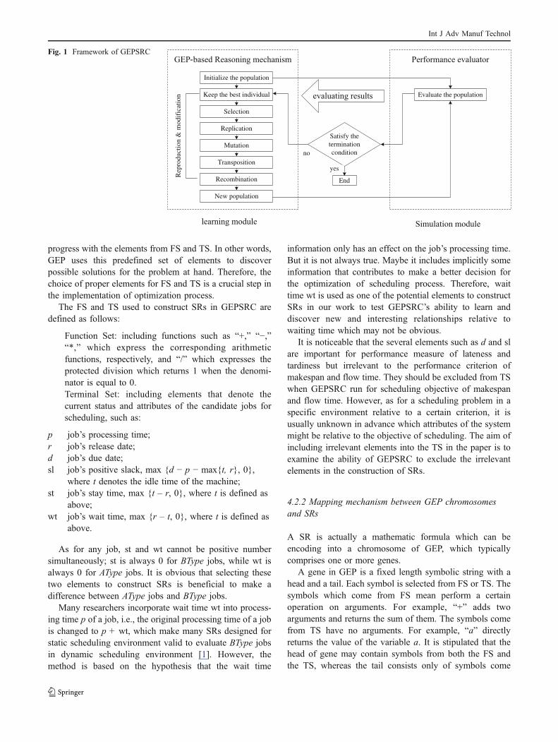
automate the process of implementing different rules andevaluating their performance using the simulation experi-ments. The simulation module works as a performanceevaluator, and the learning module uses GEP as itsreasoning mechanism to evolve SRs based on the evaluat-ing results passed back from the simulation module. Theframework of GEPSRC is shown in Fig. 1.

GEPSRC starts with an initial population which consists ofa number of candidate scheduling rules that are randomlygenerated. These rules are passed to the simulation modulethat describes the production environment and assessed usingone or more quantitative measures of performance. Then, thevalues of the performance measures for all candidate rules arepassed back to the learningmodule, where the next populationof rules is reproduced and modified from the current high-performing rules using evolutionary search operators such asselection with elitism strategy, replication, mutation, andtransposition (see Section 4.2.3). This next set of rules isthen passed to the simulation module so that the performanceof the new rules can be evaluated. This cycle is repeated untilthe termination condition is satisfied.

4.2 Application of GEPSRC on DSMSPs with job releasedates

The reasoning mechanism to explore the space of possibleSRs in GEPSRC is GEP. GEP is a new technique of creatingcomputer programs based on principle of evolution, firstlyproposed by Ferreira [40]. Like GAs [11] and GP [32], it isalso an evolutionary algorithm as it uses populations ofindividuals, selects them according to fitness, and introducesgenetic variation using one or more genetic operators [40].GEP is a genome/phenome evolutionary algorithm, whichcombines the simplicity of GAs and the abilities of GP [40].In a sense, GEP is a generalization of GAs and GP [41].GEP uses fixed length, linear strings of chromosomes(genome) to represent expression trees (ETs) of differentshapes and sizes (phenome), which makes GEP moreversatile than other evolutionary algorithms [40]. Eachchromosome is composed of elements from functions set(FS) and terminal set (TS) relevant to a particular problemdomain. The set of available elements is defined a priori. Allof the chromosomes that can be constructed using theelement set compose the search space.

The remainder of the section presents the design of FSand TS, mapping mechanism between GEP chromosomesand SRs, and operation of evolutionary search operators ofGEP and fitness function.

4.2.1 Designing of FS and TS

Each chromosome of GEP is generated randomly at thebeginning of the search and modified during evolutionary

Int J Adv Manuf Technol

progress with the elements from FS and TS. In other words,GEP uses this predefined set of elements to discoverpossible solutions for the problem at hand. Therefore, thechoice of proper elements for FS and TS is a crucial step inthe implementation of optimization process.

The FS and TS used to construct SRs in GEPSRC aredefined as follows:

Function Set: including functions such as “+,” “−,”“*,” which express the corresponding arithmeticfunctions, respectively, and “/” which expresses theprotected division which returns 1 when the denomi-nator is equal to 0.Terminal Set: including elements that denote thecurrent status and attributes of the candidate jobs forscheduling, such as:

p job’s processing time;r job’s release date;d job’s due date;sl job’s positive slack, max {d − p − max{t, r}, 0},

where t denotes the idle time of the machine;st job’s stay time, max {t – r, 0}, where t is defined as

above;wt job’s wait time, max {r – t, 0}, where t is defined as

above.

As for any job, st and wt cannot be positive numbersimultaneously; st is always 0 for BType jobs, while wt isalways 0 for AType jobs. It is obvious that selecting thesetwo elements to construct SRs is beneficial to make adifference between AType jobs and BType jobs.

Many researchers incorporate wait time wt into process-ing time p of a job, i.e., the original processing time of a jobis changed to p + wt, which make many SRs designed forstatic scheduling environment valid to evaluate BType jobsin dynamic scheduling environment [1]. However, themethod is based on the hypothesis that the wait time

information only has an effect on the job’s processing time.But it is not always true. Maybe it includes implicitly someinformation that contributes to make a better decision forthe optimization of scheduling process. Therefore, waittime wt is used as one of the potential elements to constructSRs in our work to test GEPSRC’s ability to learn anddiscover new and interesting relationships relative towaiting time which may not be obvious.

It is noticeable that the several elements such as d and slare important for performance measure of lateness andtardiness but irrelevant to the performance criterion ofmakespan and flow time. They should be excluded from TSwhen GEPSRC run for scheduling objective of makespanand flow time. However, as for a scheduling problem in aspecific environment relative to a certain criterion, it isusually unknown in advance which attributes of the systemmight be relative to the objective of scheduling. The aim ofincluding irrelevant elements into the TS in the paper is toexamine the ability of GEPSRC to exclude the irrelevantelements in the construction of SRs.

4.2.2 Mapping mechanism between GEP chromosomesand SRs

A SR is actually a mathematic formula which can beencoding into a chromosome of GEP, which typicallycomprises one or more genes.

A gene in GEP is a fixed length symbolic string with ahead and a tail. Each symbol is selected from FS or TS. Thesymbols which come from FS mean perform a certainoperation on arguments. For example, “+” adds twoarguments and returns the sum of them. The symbols comefrom TS have no arguments. For example, “a” directlyreturns the value of the variable a. It is stipulated that thehead of gene may contain symbols from both the FS andthe TS, whereas the tail consists only of symbols come

Initialize the population

Satisfy the terminationcondition

Keep the best individual

Selection

Replication

Mutation

Transposition

New population

End

yes

no

Recombination

Evaluate the population

Rep

rodu

ctio

n &

mod

ific

atio

n

Fig. 1 Framework of GEPSRC

Int J Adv Manuf Technol

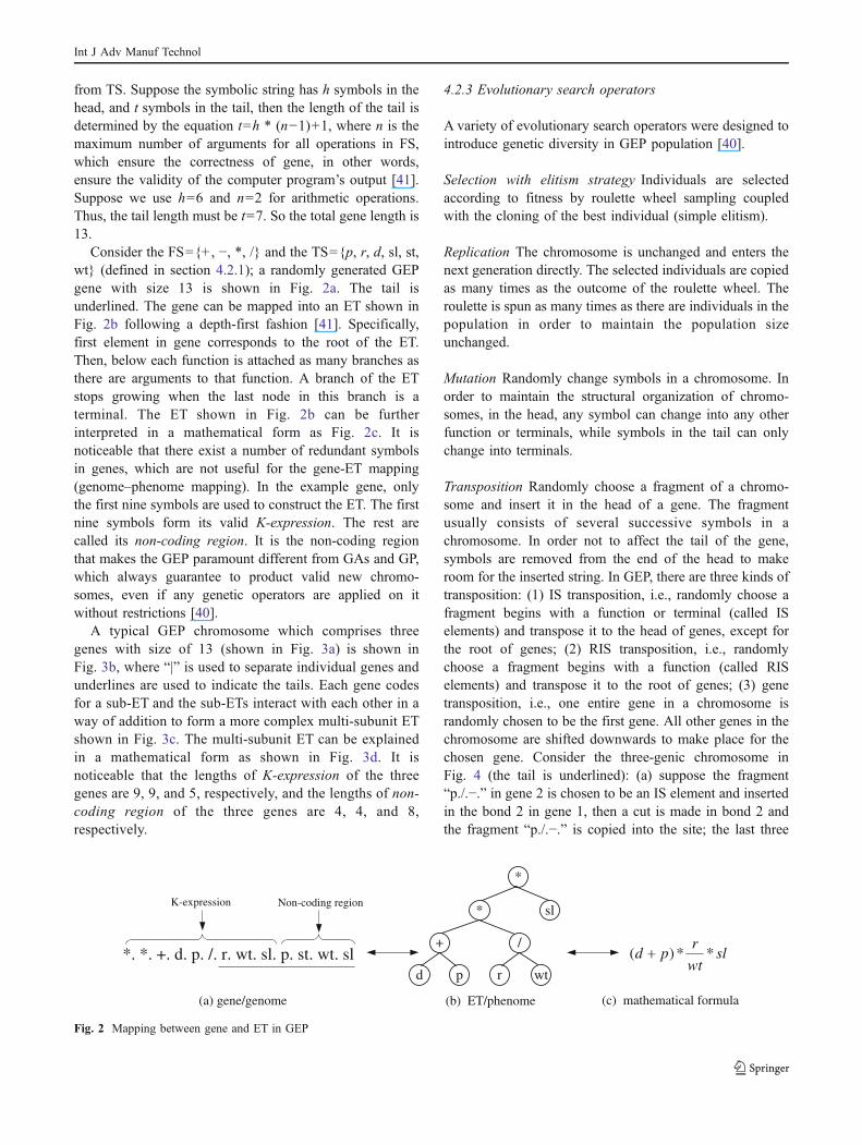
from TS. Suppose the symbolic string has h symbols in thehead, and t symbols in the tail, then the length of the tail isdetermined by the equation t=h * (n−1)+1, where n is themaximum number of arguments for all operations in FS,which ensure the correctness of gene, in other words,ensure the validity of the computer program’s output [41].Suppose we use h=6 and n=2 for arithmetic operations.Thus, the tail length must be t=7. So the total gene length is13.

Consider the FS={+, −, *, /} and the TS={p, r, d, sl, st,wt} (defined in section 4.2.1); a randomly generated GEPgene with size 13 is shown in Fig. 2a. The tail isunderlined. The gene can be mapped into an ET shown inFig. 2b following a depth-first fashion [41]. Specifically,first element in gene corresponds to the root of the ET.Then, below each function is attached as many branches asthere are arguments to that function. A branch of the ETstops growing when the last node in this branch is aterminal. The ET shown in Fig. 2b can be furtherinterpreted in a mathematical form as Fig. 2c. It isnoticeable that there exist a number of redundant symbolsin genes, which are not useful for the gene-ET mapping(genome–phenome mapping). In the example gene, onlythe first nine symbols are used to construct the ET. The firstnine symbols form its valid K-expression. The rest arecalled its non-coding region. It is the non-coding regionthat makes the GEP paramount different from GAs and GP,which always guarantee to product valid new chromo-somes, even if any genetic operators are applied on itwithout restrictions [40].

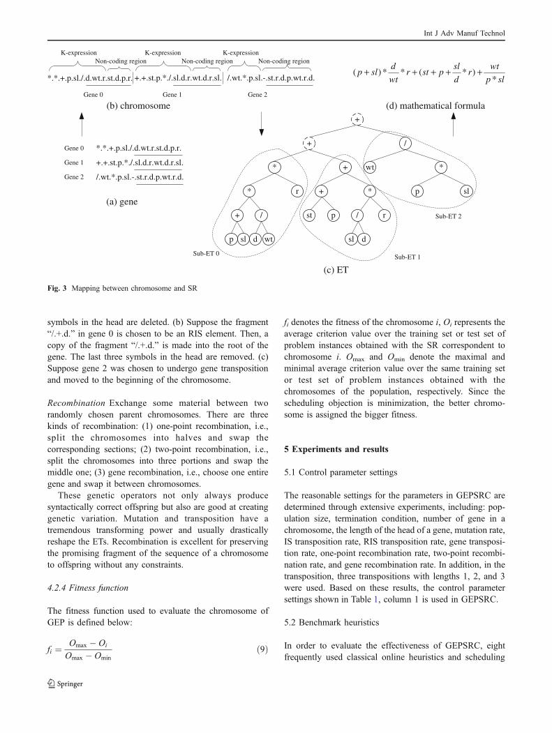
A typical GEP chromosome which comprises threegenes with size of 13 (shown in Fig. 3a) is shown inFig. 3b, where “|” is used to separate individual genes andunderlines are used to indicate the tails. Each gene codesfor a sub-ET and the sub-ETs interact with each other in away of addition to form a more complex multi-subunit ETshown in Fig. 3c. The multi-subunit ET can be explainedin a mathematical form as shown in Fig. 3d. It isnoticeable that the lengths of K-expression of the threegenes are 9, 9, and 5, respectively, and the lengths of non-coding region of the three genes are 4, 4, and 8,respectively.

4.2.3 Evolutionary search operators

A variety of evolutionary search operators were designed tointroduce genetic diversity in GEP population [40].

Selection with elitism strategy Individuals are selectedaccording to fitness by roulette wheel sampling coupledwith the cloning of the best individual (simple elitism).

Replication The chromosome is unchanged and enters thenext generation directly. The selected individuals are copiedas many times as the outcome of the roulette wheel. Theroulette is spun as many times as there are individuals in thepopulation in order to maintain the population sizeunchanged.

Mutation Randomly change symbols in a chromosome. Inorder to maintain the structural organization of chromo-somes, in the head, any symbol can change into any otherfunction or terminals, while symbols in the tail can onlychange into terminals.

Transposition Randomly choose a fragment of a chromo-some and insert it in the head of a gene. The fragmentusually consists of several successive symbols in achromosome. In order not to affect the tail of the gene,symbols are removed from the end of the head to makeroom for the inserted string. In GEP, there are three kinds oftransposition: (1) IS transposition, i.e., randomly choose afragment begins with a function or terminal (called ISelements) and transpose it to the head of genes, except forthe root of genes; (2) RIS transposition, i.e., randomlychoose a fragment begins with a function (called RISelements) and transpose it to the root of genes; (3) genetransposition, i.e., one entire gene in a chromosome israndomly chosen to be the first gene. All other genes in thechromosome are shifted downwards to make place for thechosen gene. Consider the three-genic chromosome inFig. 4 (the tail is underlined): (a) suppose the fragment“p./.−.” in gene 2 is chosen to be an IS element and insertedin the bond 2 in gene 1, then a cut is made in bond 2 andthe fragment “p./.−.” is copied into the site; the last three

*

rpd

/+

*

*. *. +. d. p. /. r. wt. sl. p. st. wt. sl

(a) gene/genome (b) ET/phenome

K-expression Non-coding region

wt

sl

( )* *r

d p slwt

(c) mathematical formula

Fig. 2 Mapping between gene and ET in GEP

Int J Adv Manuf Technol

symbols in the head are deleted. (b) Suppose the fragment“/.+.d.” in gene 0 is chosen to be an RIS element. Then, acopy of the fragment “/.+.d.” is made into the root of thegene. The last three symbols in the head are removed. (c)Suppose gene 2 was chosen to undergo gene transpositionand moved to the beginning of the chromosome.

Recombination Exchange some material between tworandomly chosen parent chromosomes. There are threekinds of recombination: (1) one-point recombination, i.e.,split the chromosomes into halves and swap thecorresponding sections; (2) two-point recombination, i.e.,split the chromosomes into three portions and swap themiddle one; (3) gene recombination, i.e., choose one entiregene and swap it between chromosomes.

These genetic operators not only always producesyntactically correct offspring but also are good at creatinggenetic variation. Mutation and transposition have atremendous transforming power and usually drasticallyreshape the ETs. Recombination is excellent for preservingthe promising fragment of the sequence of a chromosometo offspring without any constraints.

4.2.4 Fitness function

The fitness function used to evaluate the chromosome ofGEP is defined below:

fi ¼ Omax � Oi

Omax � Ominð9Þ

fi denotes the fitness of the chromosome i, Oi represents theaverage criterion value over the training set or test set ofproblem instances obtained with the SR correspondent tochromosome i. Omax and Omin denote the maximal andminimal average criterion value over the same training setor test set of problem instances obtained with thechromosomes of the population, respectively. Since thescheduling objection is minimization, the better chromo-some is assigned the bigger fitness.

5 Experiments and results

5.1 Control parameter settings

The reasonable settings for the parameters in GEPSRC aredetermined through extensive experiments, including: pop-ulation size, termination condition, number of gene in achromosome, the length of the head of a gene, mutation rate,IS transposition rate, RIS transposition rate, gene transposi-tion rate, one-point recombination rate, two-point recombi-nation rate, and gene recombination rate. In addition, in thetransposition, three transpositions with lengths 1, 2, and 3were used. Based on these results, the control parametersettings shown in Table 1, column 1 is used in GEPSRC.

5.2 Benchmark heuristics

In order to evaluate the effectiveness of GEPSRC, eightfrequently used classical online heuristics and scheduling

*.*.+.p.sl./.d.wt.r.st.d.p.r.

+.+.st.p.*./.sl.d.r.wt.d.r.sl.

/.wt.*.p.sl.-.st.r.d.p.wt.r.d.

*.*.+.p.sl./.d.wt.r.st.d.p.r. +.+.st.p.*./.sl.d.r.wt.d.r.sl. /.wt.*.p.sl.-.st.r.d.p.wt.r.d.

+

+r **

+*

/

+

slp

/

wtd

rst p

dsl

+

/

wt *

p sl

Gene 0

Gene 1

Gene 2

Sub-ET 0 Sub-ET 1

Sub-ET 2

Gene 0 Gene 1 Gene 2

(a) gene

(b) chromosome

(c) ET

K-expression K-expression K-expressionNon-coding region Non-coding region Non-coding region

( ) * * ( * )*

d sl wtp sl r st p r

wt d p sl+ + + + +

(d) mathematical formula

Fig. 3 Mapping between chromosome and SR

Int J Adv Manuf Technol

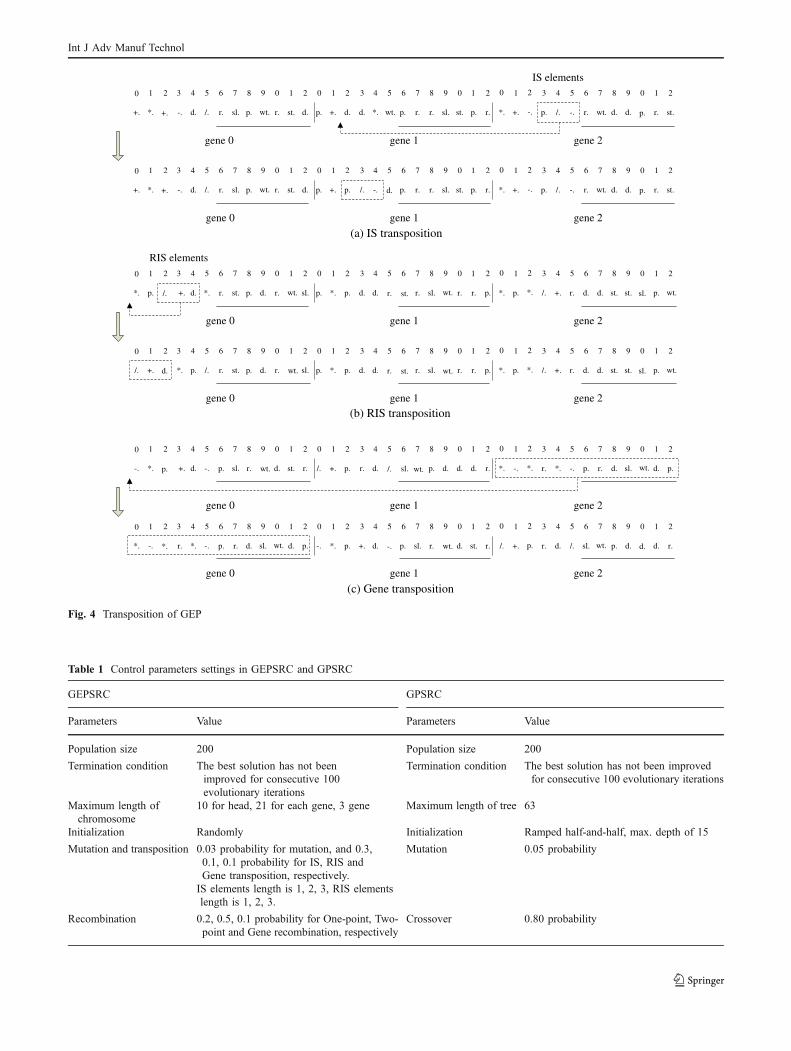
Table 1 Control parameters settings in GEPSRC and GPSRC

GEPSRC GPSRC

Parameters Value Parameters Value

Population size 200 Population size 200

Termination condition The best solution has not beenimproved for consecutive 100evolutionary iterations

Termination condition The best solution has not been improvedfor consecutive 100 evolutionary iterations

Maximum length ofchromosome

10 for head, 21 for each gene, 3 gene Maximum length of tree 63

Initialization Randomly Initialization Ramped half-and-half, max. depth of 15

Mutation and transposition 0.03 probability for mutation, and 0.3,0.1, 0.1 probability for IS, RIS andGene transposition, respectively.

Mutation 0.05 probability

IS elements length is 1, 2, 3, RIS elementslength is 1, 2, 3.

Recombination 0.2, 0.5, 0.1 probability for One-point, Two-point and Gene recombination, respectively

Crossover 0.80 probability

0 1 2 3 4 5 6 7 8 9 0 1 2 0 1 2 3 4 5 6 7 8 9

-. *. p. +. d. -. p. sl. r. wt. d. st. r. /. +. p. r. d. /. sl. wt. p. d.

0 1 2 0 1 2 3 4 5 6 7 8 9 0 1 2

d. d. r. *. -. *. r. *. -. p. r. d. sl. wt. d. p.

0 1 2 3 4 5 6 7 8 9 0 1 2 0 1 2 3 4 5 6 7 8 9

*. -. *. r. *. -. p. r. d. sl. wt. d. p. -. *. p. +. d. -. p. sl. r. wt.

0 1 2 0 1 2 3 4 5 6 7 8 9 0 1 2

d. st. r. /. +. p. r. d. /. sl. wt. p. d. d. d. r.

(c) Gene transposition

0 1 2 3 4 5 6 7 8 9 0 1 2 0 1 2 3 4 5 6 7 8 9

+. *. +. -. d. /. r. sl. p. wt. r. st. d. p. +. d. d. *. wt. p. r. r. sl.

0 1 2 0 1 2 3 4 5 6 7 8 9 0 1 2

st. p. r. *. +. -. p. /. -. r. wt. d. d. p. r. st.

0 1 2 3 4 5 6 7 8 9 0 1 2 0 1 2 3 4 5 6 7 8 9

+. *. +. -. d. /. r. sl. p. wt. r. st. d. p. +. p. /. -. d. p. r. r. sl.

0 1 2 0 1 2 3 4 5 6 7 8 9 0 1 2

st. p. r. *. +. -. p. /. -. r. wt. d. d. p. r. st.

(a) IS transposition

IS elements

0 1 2 3 4 5 6 7 8 9 0 1 2 0 1 2 3 4 5 6 7 8 9

*. p. /. +. d. *. r. st. p. d. r. wt. sl. p. *. p. d. d. r. st. r. sl. wt.

0 1 2 0 1 2 3 4 5 6 7 8 9 0 1 2

r. r. p. *. p. *. /. +. r. d. d. st. st. sl. p. wt.

0 1 2 3 4 5 6 7 8 9 0 1 2 0 1 2 3 4 5 6 7 8 9

/. +. d. *. p. /. r. st. p. d. r. wt. sl. p. *. p. d. d. r. st. r. sl. wt.

0 1 2 0 1 2 3 4 5 6 7 8 9 0 1 2

r. r. p. *. p. *. /. +. r. d. d. st. st. sl. p. wt.

RIS elements

(b) RIS transposition

gene 0 gene 1 gene 2

gene 0 gene 1 gene 2

gene 0

gene 0 gene 1

gene 1 gene 2

gene 2

gene 0

gene 0 gene 1

gene 1 gene 2

gene 2

Fig. 4 Transposition of GEP

Int J Adv Manuf Technol

rules are selected as benchmarks to which the rulesconstructed with GEPSRC are compared.

List (list scheduling) Given a set of jobs with release dates,the jobs are ordered in arbitrary list (sequence). Wheneverthe machine is idle, the first job on the list which isavailable is scheduled on the machine [13]. This algorithmworks in the model with release dates since it does not usethe information about processing times of jobs [20].

Modified PSW algorithm The algorithm produces non-preemptive schedules from preemptive ones. Given a setof jobs with release dates and processing times, apreemptive schedule is first formed using the SRPT rule.Under this rule, the machine always picks jobs with theshortest remaining processing time among those alreadyreleased at the current time and processes these first. Eachjob will have a (preemptive) completion time Cj. Next, anordered list L of jobs is formed based on their preemptivecompletion time Cj using a simple sort. A non-preemptiveschedule is then obtained if the first job in L is continued tobe assigned to the machine when it is freed and delete itfrom L. The algorithm yields good solutions for theproblem on average [19].

Earliest due date rule All jobs currently waiting processingin the queue of the machine are listed in ascending order oftheir due dates di. The first job in the list is processed nextat the machine. This rule is the most popular due-date-based rule. It is known to be used as a benchmark forreducing maximum tardiness and variance of tardiness [42].

Montagne rule Montagne rule (MON) sequences jobscurrently waiting processing in ascending order of thefollowing ratio pi/(P–di), where P denotes the sum of theprocessing time of all jobs [43]. The first job in the list isprocessed next at the machine. This means that a job with adue date close to the sum of the processing time of all jobsis likely to be scheduled on a later stage. Conversely, jobswith early due dates are given extra priority. MON performswell on different types of single-machine tardiness prob-lems [33].

Minimum slack time rule Minimum slack time rule (MST)lists jobs currently waiting for processing in ascendingorder of their slack sli, where slack for a job is computed bysubtracting its processing time at the machine pi and thecurrent time t from its due date di, i.e., sli=di– t–pi. Thefirst job in the list is processed next at the machine. Thisrule is also used to reduce total tardiness of jobs [44].

Modified due date rule The jobs are listed in ascendingorder of their modified due date mdi, where the modified

due date of a job is the maximum of its due date and itsremaining processing time, i.e., mdi=max (t+pi, di). Thismeans that once a job becomes critical, its due datebecomes its earliest completion time. The first job in thelist is processed next at the machine. This rule is aimed tominimize total tardiness of jobs [45].

Cost over time rule When a job is projected to be tardy(i.e., its slack is 0), its priority value reduces to 1/pi. On theother hand, if a job is expected to be very early where theslack exceeds an estimation of the delay cost, the priorityvalue for the job increases linearly with decreases in slack.Cost over time rule (COVERT) uses a worst-case estimateof delay as the job processing times multiplied by a look-ahead parameter k. In other words, the priority value of jobi is computed as 1

pi� 1� di�t�pið Þþ

k�pi

� �þ, where (X)

+=max(0, X)

[46]. Thus, the priority value of a job increases linearlyfrom 0 when slack is very high to 1/pi when the status ofjob becomes tardy. The job with the largest COVERTpriority value is processed next at the machine.

Apparent tardiness cost rule Apparent tardiness cost rule(ATC), a modification of COVERT, estimates the delaypenalty using an exponential discounting formulation, i.e.,

priority value of job i is computed with 1pi� e�

di�t�pið Þþk�pi [47].

If a job is tardy, ATC reduces to 1/pi. If the job experiencesvery high slack, ATC reduces to the MST. It must be notedthat if the estimated delay is extremely large, ATC againreduces to 1/pi, which is different from COVERT. The jobwith the largest priority value is processed next at themachine.

In both COVERT and ATC, the look-ahead factor kcan significantly affect performance; k is varied from 0.5to 4.5 in increments of 0.5, and the objective functionvalue where COVERT and ATC each performs best isrecorded.

GPRules GP-based scheduling approaches which automat-ically construct effective rules for a given schedulingenvironment have been investigated recently, and they haveachieved good performance [1, 31, 33-39]. Therefore,besides the classical online heuristics and scheduling rulesmentioned above, the rules evolved by GP are also used toevaluate the efficiency of GEPSRC. In the paper, GP-basedscheduling rules constructor (GPSRC) is also implementedin which GP is used as the reasoning mechanism to searchthe SRs space. The description of GPSRC is provided in theAppendix. The control parameters settings for GPSRC aresummarized in Table 1, column 2. It is noticeable that anindividual of GP is represented as a rooted tree, while anindividual of GEP map into several sub-trees which areconnected with each other to form a bigger tree as describein Section 4.2.2. It is unique character of GEP that an

Int J Adv Manuf Technol

individual may consist of more than one gene, whichsignificantly improve the expression ability of the geno-type/phenotype. But a maximum program size of 63 wasused in both GP and GEP so that comparisons could bemade between all the experiments (to be more precise, forGEP with three genes with head length 10, maximumprogram size of GEP equals 63).

The measure used for heuristic comparison is thepercent-relative error computed as

%Error ¼ Ok � Ol

Ol

Where Ok is the average objective value over the test set ofproblem instances obtain by heuristic k, and Ol is theaverage objective value over the test set of probleminstances obtain by heuristic l. A negative value indicatesthat heuristic k performs better than heuristic l.

5.3 Design of experiments

In this section, we generate a series of training sets and testsets that represent a set of problem instances of varyingoperating conditions to evolve rules with GEPSRC andevaluate them.

Problem instances are randomly generated with theinstance generation approach used by Jakobovic and Budi[1]. Each scheduling problem instance is defined with thefollowing parameters:

n the number of jobs. Its value is 10, 50, or 100;pj processing time of job j, j=1,…, n. The values of

processing time are assumed as integers and drawn outof U[1,100], U[100, 200], or U[200, 300], where Urefers to the uniform distribution;

rj release date of job j, j=1,…, n. Release dates areintegers chosen randomly from U[0, 1/2 * P], where Urefers to the uniform distribution and P denotes thesum of the processing time of all jobs;

dj due date of job j, j=1,…, n. Due dates are integers anddrawn out of U rj þ P � rj

� �» 1� T � R=2ð Þ; rjþ

�P � rj� �

» 1� T þ R=2ð Þ�, where U refers to theuniform distribution, P denotes the sum of theprocessing time of all jobs, T is due date tightnessfactor which represents the expected percentage of latejobs, and R is due date range factor which defines thedispersion of the due dates values. T and R areassigned values of 0.1, 0.5, or 0.9.

wj weight of job j, j=1,…, n. We assume all jobsrelatively equal, i.e., wj=1.

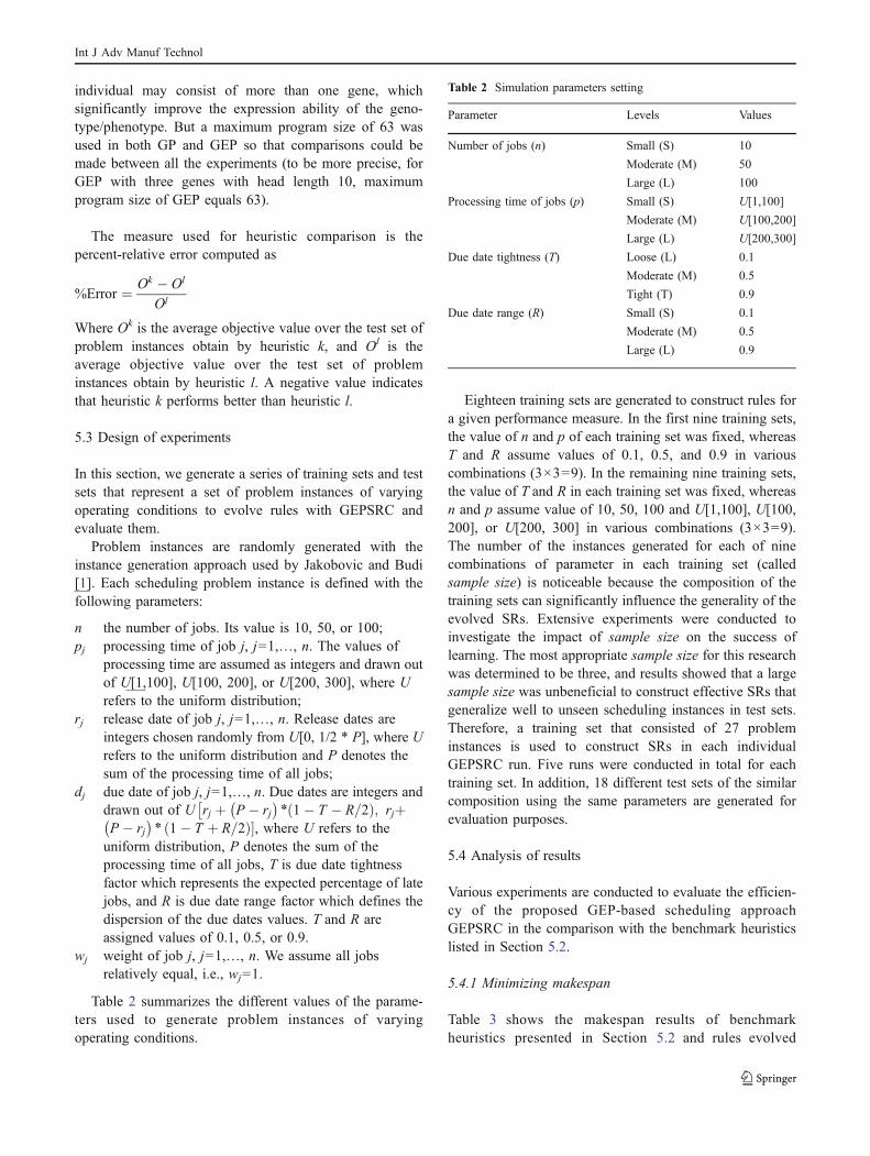
Table 2 summarizes the different values of the parame-ters used to generate problem instances of varyingoperating conditions.

Eighteen training sets are generated to construct rules fora given performance measure. In the first nine training sets,the value of n and p of each training set was fixed, whereasT and R assume values of 0.1, 0.5, and 0.9 in variouscombinations (3×3=9). In the remaining nine training sets,the value of T and R in each training set was fixed, whereasn and p assume value of 10, 50, 100 and U[1,100], U[100,200], or U[200, 300] in various combinations (3×3=9).The number of the instances generated for each of ninecombinations of parameter in each training set (calledsample size) is noticeable because the composition of thetraining sets can significantly influence the generality of theevolved SRs. Extensive experiments were conducted toinvestigate the impact of sample size on the success oflearning. The most appropriate sample size for this researchwas determined to be three, and results showed that a largesample size was unbeneficial to construct effective SRs thatgeneralize well to unseen scheduling instances in test sets.Therefore, a training set that consisted of 27 probleminstances is used to construct SRs in each individualGEPSRC run. Five runs were conducted in total for eachtraining set. In addition, 18 different test sets of the similarcomposition using the same parameters are generated forevaluation purposes.

5.4 Analysis of results

Various experiments are conducted to evaluate the efficien-cy of the proposed GEP-based scheduling approachGEPSRC in the comparison with the benchmark heuristicslisted in Section 5.2.

5.4.1 Minimizing makespan

Table 3 shows the makespan results of benchmarkheuristics presented in Section 5.2 and rules evolved

Table 2 Simulation parameters setting

Parameter Levels Values

Number of jobs (n) Small (S) 10

Moderate (M) 50

Large (L) 100

Processing time of jobs (p) Small (S) U[1,100]

Moderate (M) U[100,200]

Large (L) U[200,300]

Due date tightness (T) Loose (L) 0.1

Moderate (M) 0.5

Tight (T) 0.9

Due date range (R) Small (S) 0.1

Moderate (M) 0.5

Large (L) 0.9

Int J Adv Manuf Technol

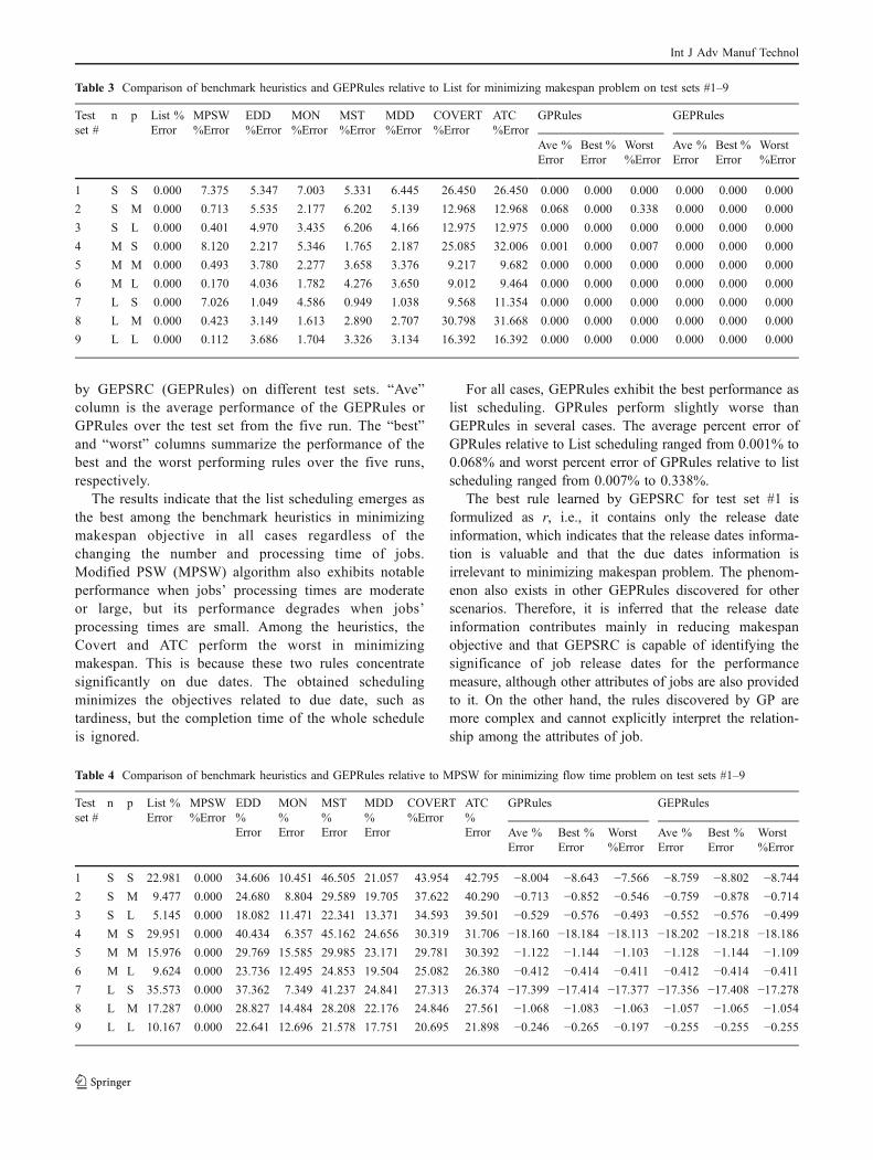
by GEPSRC (GEPRules) on different test sets. “Ave”column is the average performance of the GEPRules orGPRules over the test set from the five run. The “best”and “worst” columns summarize the performance of thebest and the worst performing rules over the five runs,respectively.

The results indicate that the list scheduling emerges asthe best among the benchmark heuristics in minimizingmakespan objective in all cases regardless of thechanging the number and processing time of jobs.Modified PSW (MPSW) algorithm also exhibits notableperformance when jobs’ processing times are moderateor large, but its performance degrades when jobs’processing times are small. Among the heuristics, theCovert and ATC perform the worst in minimizingmakespan. This is because these two rules concentratesignificantly on due dates. The obtained schedulingminimizes the objectives related to due date, such astardiness, but the completion time of the whole scheduleis ignored.

For all cases, GEPRules exhibit the best performance aslist scheduling. GPRules perform slightly worse thanGEPRules in several cases. The average percent error ofGPRules relative to List scheduling ranged from 0.001% to0.068% and worst percent error of GPRules relative to listscheduling ranged from 0.007% to 0.338%.

The best rule learned by GEPSRC for test set #1 isformulized as r, i.e., it contains only the release dateinformation, which indicates that the release dates informa-tion is valuable and that the due dates information isirrelevant to minimizing makespan problem. The phenom-enon also exists in other GEPRules discovered for otherscenarios. Therefore, it is inferred that the release dateinformation contributes mainly in reducing makespanobjective and that GEPSRC is capable of identifying thesignificance of job release dates for the performancemeasure, although other attributes of jobs are also providedto it. On the other hand, the rules discovered by GP aremore complex and cannot explicitly interpret the relation-ship among the attributes of job.

Table 3 Comparison of benchmark heuristics and GEPRules relative to List for minimizing makespan problem on test sets #1–9

Testset #

n p List %Error

MPSW%Error

EDD%Error

MON%Error

MST%Error

MDD%Error

COVERT%Error

ATC%Error

GPRules GEPRules

Ave %Error

Best %Error

Worst%Error

Ave %Error

Best %Error

Worst%Error

1 S S 0.000 7.375 5.347 7.003 5.331 6.445 26.450 26.450 0.000 0.000 0.000 0.000 0.000 0.000

2 S M 0.000 0.713 5.535 2.177 6.202 5.139 12.968 12.968 0.068 0.000 0.338 0.000 0.000 0.000

3 S L 0.000 0.401 4.970 3.435 6.206 4.166 12.975 12.975 0.000 0.000 0.000 0.000 0.000 0.000

4 M S 0.000 8.120 2.217 5.346 1.765 2.187 25.085 32.006 0.001 0.000 0.007 0.000 0.000 0.000

5 M M 0.000 0.493 3.780 2.277 3.658 3.376 9.217 9.682 0.000 0.000 0.000 0.000 0.000 0.000

6 M L 0.000 0.170 4.036 1.782 4.276 3.650 9.012 9.464 0.000 0.000 0.000 0.000 0.000 0.000

7 L S 0.000 7.026 1.049 4.586 0.949 1.038 9.568 11.354 0.000 0.000 0.000 0.000 0.000 0.000

8 L M 0.000 0.423 3.149 1.613 2.890 2.707 30.798 31.668 0.000 0.000 0.000 0.000 0.000 0.000

9 L L 0.000 0.112 3.686 1.704 3.326 3.134 16.392 16.392 0.000 0.000 0.000 0.000 0.000 0.000

Table 4 Comparison of benchmark heuristics and GEPRules relative to MPSW for minimizing flow time problem on test sets #1–9

Testset #

n p List %Error

MPSW%Error

EDD%Error

MON%Error

MST%Error

MDD%Error

COVERT%Error

ATC%Error

GPRules GEPRules

Ave %Error

Best %Error

Worst%Error

Ave %Error

Best %Error

Worst%Error

1 S S 22.981 0.000 34.606 10.451 46.505 21.057 43.954 42.795 −8.004 −8.643 −7.566 −8.759 −8.802 −8.7442 S M 9.477 0.000 24.680 8.804 29.589 19.705 37.622 40.290 −0.713 −0.852 −0.546 −0.759 −0.878 −0.7143 S L 5.145 0.000 18.082 11.471 22.341 13.371 34.593 39.501 −0.529 −0.576 −0.493 −0.552 −0.576 −0.4994 M S 29.951 0.000 40.434 6.357 45.162 24.656 30.319 31.706 −18.160 −18.184 −18.113 −18.202 −18.218 −18.1865 M M 15.976 0.000 29.769 15.585 29.985 23.171 29.781 30.392 −1.122 −1.144 −1.103 −1.128 −1.144 −1.1096 M L 9.624 0.000 23.736 12.495 24.853 19.504 25.082 26.380 −0.412 −0.414 −0.411 −0.412 −0.414 −0.4117 L S 35.573 0.000 37.362 7.349 41.237 24.841 27.313 26.374 −17.399 −17.414 −17.377 −17.356 −17.408 −17.2788 L M 17.287 0.000 28.827 14.484 28.208 22.176 24.846 27.561 −1.068 −1.083 −1.063 −1.057 −1.065 −1.0549 L L 10.167 0.000 22.641 12.696 21.578 17.751 20.695 21.898 −0.246 −0.265 −0.197 −0.255 −0.255 −0.255

Int J Adv Manuf Technol

5.4.2 Minimizing flow time

Table 4 shows the flow time results of benchmark heuristicsand GEPRules on different test sets. Since MPSWalgorithm produces good solutions for the flow timeproblem, the average objective function values obtainedfrom the other heuristics, including the rules that arediscovered by GEPSRC and GPSRC, are compared tothose values form MPSW. The second rank goes to MONrule, but MON performs worse than list scheduling in thecases where the jobs’ processing time is large. Listscheduling exhibits better performance than modified duedate rule (MDD) expect for the cases where the jobs’processing time is small. The results in Table 4 indicate thatMST obtains the worst result when jobs’ processing timesare small, however, its performance increase as theprocessing time increase.

Table 4 also shows that the rules constructed byGEPSRC and GPSRC outperform MPSW algorithm in allcases, especially in the cases where the jobs’ processingtime is small. In the comparison with GPRules, GEPRulesshows better performance when the number of jobs aresmall or moderate. The improvement over MPSW obtainedfrom GEPSRC is more than that obtained from GPSRC by0.755% for the average percent error, 0.159% for the bestpercent error, and 1.178% for the worst percent error.However, GEPSRC’s performance degrades when thenumber of jobs becomes large, but these result in smalldegradation in average objective function value. Theimprovement over MPSW obtained from GEPSRC is lessthan that obtained from GPSRC by 0.043% for the averagepercent error, 0.018% for the best percent error, and 0.099%for the worst percent error.

GEPSRC exhibits the ability to intelligently select theuseful attributes from candidate ones to automaticallyconstruct effective SRs. Take the best rules constructed by

GEPSRC for test set #4 and #9 (Rule-F4 and Rule-F9) forexample.

pþ wt2 þ r � wt� wt2

pðRule� F4Þ

pþ 2wtþ r

wtðRule� F9Þ

From Rule-F4 and Rule-F9, it is easy to find that thespecific due date parameters of due date d and slack sl isnot relevant to the criterion of minimizing flow time,regardless of the variation of due dates of the jobs to bescheduled, whereas release date r and processing time phelp to reduce the flow time of the jobs (recall that from thedefinition of waiting time wt in Section 4.2.1; waiting timewt and release date r are correlated). Moreover, when alljobs are available simultaneously, the rule above may bereduced into p, i.e., SPT rule, which produces optimalsolution for the special case [14].

As for the rules discovered by GPSRC, the relationshipamong the attributes of jobs cannot be explicitly explainedfrom their expressions since they are usually quite complex.

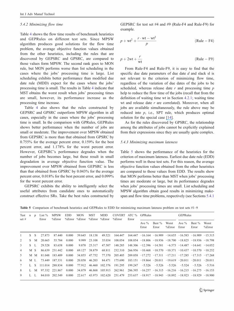
5.4.3 Minimizing maximum lateness

Table 5 shows the performance of the heuristics for thecriterion of maximum lateness. Earliest due date rule (EDD)performs well in these test sets. For this reason, the averageobjective function values obtained from the other heuristicsare compared to those values from EDD. The results showthat MON performs better than MST when jobs’ processingtimes are moderate or large, but its performance degradeswhen jobs’ processing times are small. List scheduling andMPSW algorithm obtain good results in minimizing make-span and flow time problems, respectively (see Sections 5.4.1

Table 5 Comparison of benchmark heuristics and GEPRules to EDD for minimizing maximum lateness problem on test sets #1–9

Testset #

n p List %Error

MPSW%Error

EDD%Error

MON%Error

MST%Error

MDD%Error

COVERT%Error

ATC %Error

GPRules GEPRules

Ave %Error

Best %Error

Worst%Error

Ave %Error

Best %Error

Worst%Error

1 S S 27.873 87.440 0.000 39.645 18.138 49.521 164.447 164.447 −16.164 −16.909 −14.655 −16.583 −16.909 −15.3152 S M 20.665 55.784 0.000 9.999 23.108 35.034 108.054 108.054 −18.806 −18.936 −18.700 −18.825 −18.936 −18.7983 S L 29.528 83.658 0.000 9.870 25.317 47.507 148.285 148.306 −12.396 −14.581 −6.573 −14.487 −14.641 −14.0524 M S 86.639 231.442 0.000 69.127 38.879 68.811 232.310 266.956 −10.468 −10.570 −10.371 −10.437 −10.570 −10.2525 M M 81.048 183.409 0.000 34.855 47.752 77.370 205.405 209.058 −17.272 −17.311 −17.211 −17.285 −17.315 −17.2686 M L 73.449 187.331 0.000 20.858 46.203 84.471 175.690 183.151 −19.864 −20.011 −19.619 −20.011 −20.011 −20.0117 L S 111.014 288.834 0.000 77.912 46.460 102.376 191.295 199.247 −5.526 −5.526 −5.526 −5.524 −5.526 −5.5168 L M 97.332 221.867 0.000 34.879 46.868 105.913 262.961 286.395 −16.257 −16.315 −16.216 −16.215 −16.275 −16.153

9 L L 84.010 202.549 0.000 22.617 43.973 102.620 251.479 253.637 −18.917 −18.943 −18.892 −18.923 −18.929 −18.900

Int J Adv Manuf Technol

and 5.4.2). However, they perform poorly in minimizingmaximum lateness in comparison with EDD. This is becausethe due dates of jobs are ignored by the two algorithms.COVERT and ATC perform worst among the heuristics forthe due-date-related objective, although they are also due-date-based rules. The reason is that they try to minimize thedeviation between the completion time and due date for eachjob, which may degrade the objective of minimizingmaximum lateness.

From the results, it is also easy to found that bothGEPRules and GPRules exhibit much better behave thanEDD. When the number of jobs is small and moderate,GEPSRC exhibits better performance than GPSRC, excepton the test case #4. However, the performance of GEPSRCis slightly worse than GPSRC when the number of jobs islarge. The improvement on average performance obtainedfrom GEPSRC over EDD is less than that obtained fromGPSRC by 0.042%, the improvement on best learned ruleperformance obtained from GEPSRC is less than thatobtained from GPSRC by 0.04%, and the improvementon worst learned rule performance obtained from GEPSRCis less than that obtained from GPSRC by 0.119%.

Take a closer look at the best rules constructed byGEPSRC for test set #5 and #9 (Rule-L5 and Rule-L9).

d þ p � wt2 þ r

wtðRule� L5Þ

d þ slþ r � wt ðRule� L9ÞThe learned rules show the visible role of due date-

related attribute d and sl. This seems logical, as theobjective function is due-date-related and is aligned withthe general conclusions of the scheduling research commu-nity. Moreover, when all jobs are available simultaneously,the rules above may be reduced into d, i.e., EDD rule or thecombination rule of EDD and MST. The rules discoveredby GPSRC can not explicitly explain the relationshipamong the attributes of jobs.

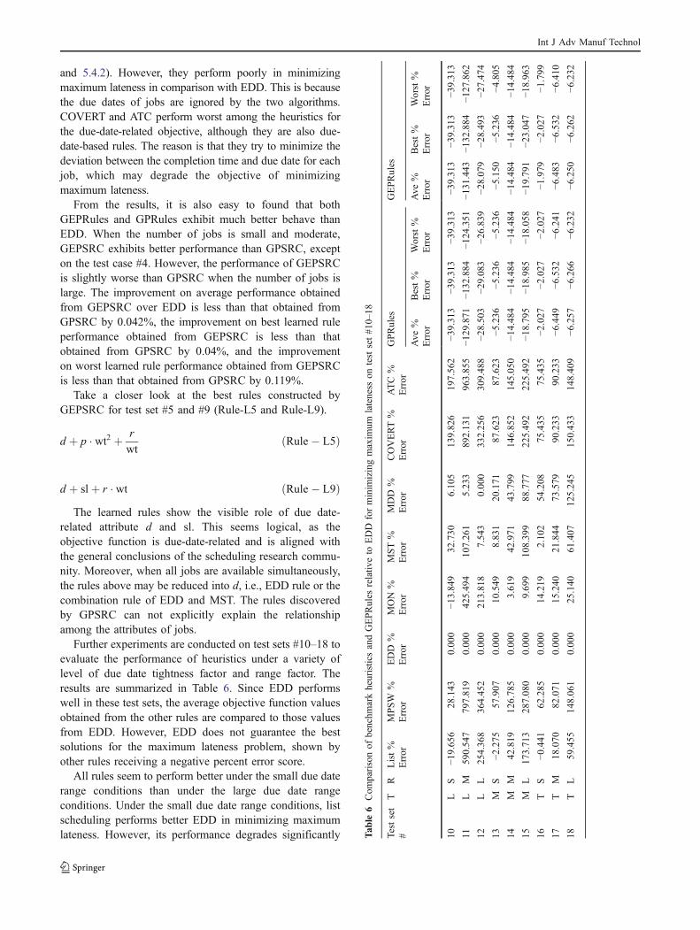
Further experiments are conducted on test sets #10–18 toevaluate the performance of heuristics under a variety oflevel of due date tightness factor and range factor. Theresults are summarized in Table 6. Since EDD performswell in these test sets, the average objective function valuesobtained from the other rules are compared to those valuesfrom EDD. However, EDD does not guarantee the bestsolutions for the maximum lateness problem, shown byother rules receiving a negative percent error score.

All rules seem to perform better under the small due daterange conditions than under the large due date rangeconditions. Under the small due date range conditions, listscheduling performs better EDD in minimizing maximumlateness. However, its performance degrades significantly T

able

6Com

parisonof

benchm

arkheuristicsandGEPRules

relativ

eto

EDD

forminim

izingmaxim

umlateness

ontestset#1

0–18

Testset

#T

RList%

Error

MPSW

%Error

EDD

%Error

MON

%Error

MST%

Error

MDD

%Error

COVERT%

Error

ATC

%Error

GPRules

GEPRules

Ave

%Error

Best%

Error

Worst%

Error

Ave

%Error

Best%

Error

Worst%

Error

10L

S−1

9.65

628

.143

0.00

0−1

3.84

932

.730

6.10

513

9.82

619

7.56

2−3

9.31

3−3

9.31

3−3

9.31

3−3

9.31

3−3

9.31

3−3

9.31

3

11L

M59

0.54

779

7.81

90.00

042

5.49

410

7.26

15.23

389

2.13

196

3.85

5−1

29.871

−132

.884

−124

.351

−131

.443

−132

.884

−127

.862

12L

L25

4.36

836

4.45

20.00

021

3.81

87.54

30.00

033

2.25

630

9.48

8−2

8.50

3−2

9.08

3−2

6.83

9−2

8.07

9−2

8.49

3−2

7.47

4

13M

S−2

.275

57.907

0.00

010

.549

8.83

120

.171

87.623

87.623

−5.236

−5.236

−5.236

−5.150

−5.236

−4.805

14M

M42

.819

126.78

50.00

03.61

942

.971

43.799

146.85

214

5.05

0−1

4.48

4−1

4.48

4−1

4.48

4− 1

4.48

4−1

4.48

4−1

4.48

4

15M

L17

3.71

328

7.08

00.00

09.69

910

8.39

988

.777

225.49

222

5.49

2−1

8.79

5−1

8.98

5−1

8.05

8−1

9.79

1−2

3.04

7−1

8.96

3

16T

S−0

.441

62.285

0.00

014

.219

2.10

254

.208

75.435

75.435

−2.027

−2.027

−2.027

−1.979

−2.027

−1.799

17T

M18

.070

82.071

0.00

015

.240

21.844

73.579

90.233

90.233

−6.449

−6.532

−6.241

−6.483

−6.532

−6.410

18T

L59

.455

148.06

10.00

025

.140

61.407

125.24

515

0.43

314

8.40

9−6

.257

−6.266

−6.232

−6.250

−6.262

−6.232

Int J Adv Manuf Technol

with the increase of due date range. Both MON and MDDoutperforms MPSW under all cases. As expected, COVERTand ATC perform well when due date are tight, but theystill perform poor compared with other heuristics.

Under all conditions, GEPRules and GPRules performmuch better than all the benchmark heuristics. In mostcases, GEPRules perform the best or tie for best. However,under larger due date range condition, the performance ofGEPRules degrades slightly, but it results in smalldegradation in the average objection values obtained byGEPRule. In the cases where the GEPRules perform worsethan GPRules, the percent error improvement relative toEDD obtained by GEPRule is less than that obtained byGPRule by 0.424% for average percent error, 0.59% forbest percent error, and 0.431% for worst percent error. Onthe cases where the GEPRules perform better thanGPRules, the percent error improvement relative to EDDobtained by GEPRules is more than that obtained byGPRules by 1.572% for average percent error, 4.062% forbest percent error, and 3.511% for worst percent error.

Take a closer look at the best rules constructed byGEPSRCfor test set 11# and 17# (Rule-L11 and Rule-L17).

2d þ slþ pþ r � wt ðRule� L11Þ

d þ d2 � wtþ wt ðRule� L17ÞThe learned rules show that under the loose due date

tightness and moderate due date range condition, i.e., on thetest set 11#, in order to minimize the maximum lateness, theparameters of d, sl, p, r, and wt all contribute to the successof the scheduling. Whereas, under the tight due datetightness and moderate due date range condition, i.e., onthe test set 17#, the d and wt play dominating rule on the

scheduling decision in order to minimizing the maximumlateness. It means that the GEPSRC can identify thecharacteristics of the operation conditions and constructappropriate rules.

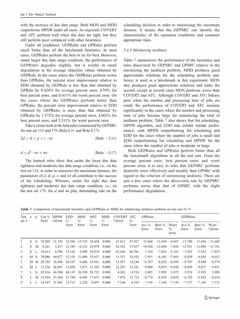
5.4.4 Minimizing tardiness

Table 7 summarizes the performance of the heuristics andrules discovered by GEPSRC and GPSRC relative to theminimizing the tardiness problem. MDD produces goodapproximate solutions for the scheduling problem and,hence, is used as a benchmark in this experiment. MONalso produces good approximate solutions and ranks thesecond, except in several cases MON performs worse thanCOVERT and ATC. Although COVERT and ATC behavepoor when the number and processing time of jobs aresmall, the performance of COVERT and ATC increasesignificantly in the cases where the number and processingtime of jobs become large for minimizing the total oftardiness problem. Table 7 also shows that list scheduling,MPSW algorithm, and EDD rule exhibit similar perfor-mance, with MPSW outperforming list scheduling andEDD for the cases where the number of jobs is small andEDD outperforming list scheduling and MPSW for thecases where the number of jobs is moderate or large.

Both GEPRules and GPRules perform better than allthe benchmark algorithms in all the test sets. From theaverage percent error, best percent error, and worstpercent error, it is easy to infer that GEPSRC performsdistinctly more effectively and steadily than GPSRC withregard to the criterion of minimizing tardiness. There arejust a few cases where the discovered rule by GEPSRCperforms worse than that of GPSRC with the slightperformance degradation.

Table 7 Comparison of benchmark heuristics and GEPRules to MDD for minimizing tardiness problem on test sets #1–9

Testset #

n p List %Error

MPSW%Error

EDD%Error

MON%Error

MST%Error

MDD%Error

COVERT%Error

ATC%Error

GPRules GEPRules

Ave %Error

Best %Error

Worst%Error

Ave %Error

Best %Error

Worst%Error

1 S S 32.905 21.195 32.596 15.579 38.458 0.000 47.613 47.427 −11.068 −11.836 −8.687 −11.760 −11.836 −11.6042 S M 8.261 2.427 12.349 −0.316 16.878 0.000 36.301 37.037 −10.926 −12.094 −7.038 −11.951 −12.094 −11.7913 S L 10.613 8.596 13.142 2.090 10.978 0.000 45.246 48.701 −7.320 −7.853 −5.191 −7.853 −7.853 −7.8534 M S 78.086 60.877 57.193 31.009 55.637 0.000 15.351 18.593 −7.951 −8.183 −7.693 −8.029 −8.034 −8.0125 M M 28.703 26.888 20.247 6.646 16.441 0.000 13.957 14.244 −8.767 −8.829 −8.694 −8.797 −8.944 −8.5746 M L 21.236 26.891 13.058 1.871 11.303 0.000 12.297 13.241 −9.060 −9.074 −9.038 −9.039 −9.071 −9.0317 L S 82.816 66.504 48.147 36.350 50.712 0.000 4.262 4.210 −3.891 −3.995 −3.475 −3.974 −3.995 −3.8898 L M 33.564 35.504 21.794 6.445 17.071 0.000 7.478 12.713 −6.774 −6.859 −6.639 −6.742 −6.859 −6.6349 L L 24.347 31.903 15.712 2.238 9.697 0.000 7.394 8.393 −7.156 −7.168 −7.139 −7.157 −7.185 −7.113

Int J Adv Manuf Technol

The best rule evolved by GEPSRC for test sets 3# and7# (Rule-T3 and Rule-T7) is shown below.

slþ 2pþ r � wt � p ðRule� T3Þ

slþ pþ wtþ wt2 ðRule� T7ÞFrom the formula of Rule-T3 and Rule-T7, it is found

that the GEPSRC picks the sl as an indispensable elementto construct SRs for the scheduling decision relative to thecriterion of tardiness. Essentially, the first term of sl worksas MST rule, which performs well under the performancemeasure of tardiness. Besides sl, it is noticeable that p and ralso play an important role for the scheduling decision. Therules discovered by GPSRC cannot explicitly explain therelationship among the attributes of jobs.

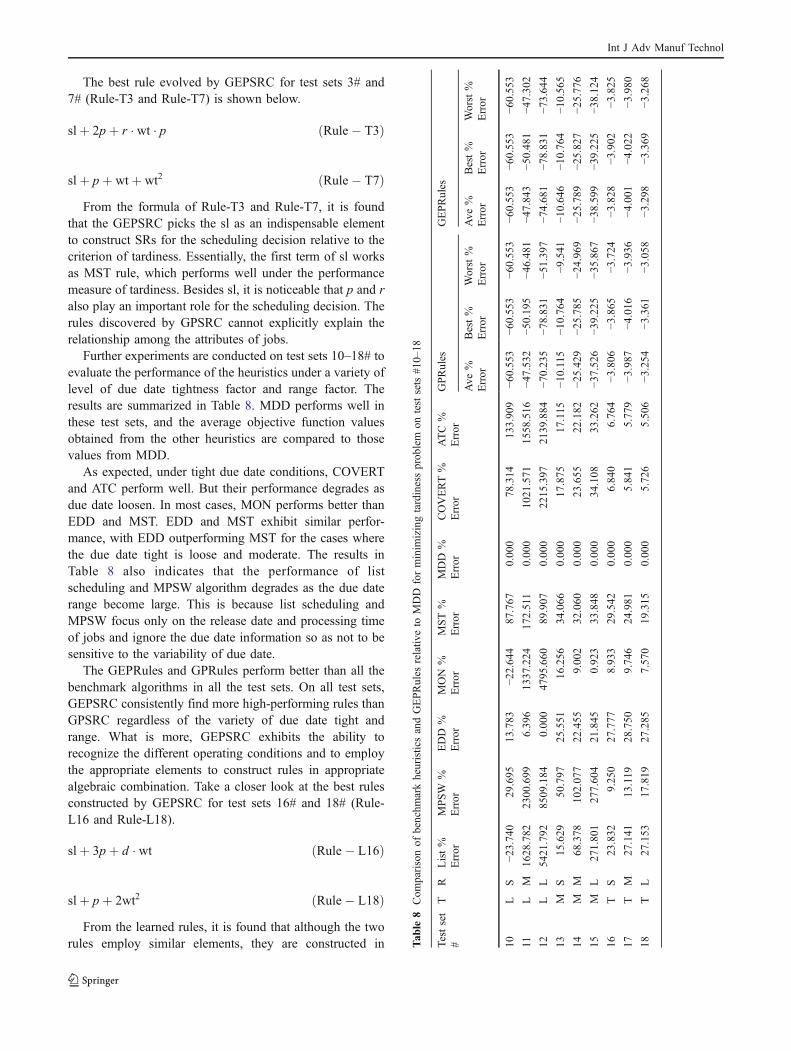
Further experiments are conducted on test sets 10–18# toevaluate the performance of the heuristics under a variety oflevel of due date tightness factor and range factor. Theresults are summarized in Table 8. MDD performs well inthese test sets, and the average objective function valuesobtained from the other heuristics are compared to thosevalues from MDD.

As expected, under tight due date conditions, COVERTand ATC perform well. But their performance degrades asdue date loosen. In most cases, MON performs better thanEDD and MST. EDD and MST exhibit similar perfor-mance, with EDD outperforming MST for the cases wherethe due date tight is loose and moderate. The results inTable 8 also indicates that the performance of listscheduling and MPSW algorithm degrades as the due daterange become large. This is because list scheduling andMPSW focus only on the release date and processing timeof jobs and ignore the due date information so as not to besensitive to the variability of due date.

The GEPRules and GPRules perform better than all thebenchmark algorithms in all the test sets. On all test sets,GEPSRC consistently find more high-performing rules thanGPSRC regardless of the variety of due date tight andrange. What is more, GEPSRC exhibits the ability torecognize the different operating conditions and to employthe appropriate elements to construct rules in appropriatealgebraic combination. Take a closer look at the best rulesconstructed by GEPSRC for test sets 16# and 18# (Rule-L16 and Rule-L18).

slþ 3pþ d � wt ðRule� L16Þ

slþ pþ 2wt2 ðRule� L18ÞFrom the learned rules, it is found that although the two

rules employ similar elements, they are constructed in Tab

le8

Com

parisonof

benchm

arkheuristicsandGEPRules

relativ

eto

MDD

forminim

izingtardinessprob

lem

ontestsets#1

0–18

Testset

#T

RList%

Error

MPSW

%Error

EDD

%Error

MON

%Error

MST%

Error

MDD

%Error

COVERT%

Error

ATC%

Error

GPRules

GEPRules

Ave

%Error

Best%

Error

Worst%

Error

Ave

%Error

Best%

Error

Worst%

Error

10L

S−2

3.74

029

.695

13.783

−22.64

487

.767

0.00

078

.314

133.90

9−6

0.55

3−6

0.55

3−6

0.55

3−6

0.55

3−6

0.55

3−6

0.55

3

11L

M16

28.782

2300

.699

6.39

613

37.224

172.511

0.00

010

21.571

1558

.516

−47.53

2−5

0.19

5−4

6.48

1−4

7.84

3−5

0.48

1−4

7.30

2

12L

L54

21.792

8509

.184

0.00

047

95.660

89.907

0.00

022

15.397

2139

.884

−70.23

5−7

8.83

1−5

1.39

7−7

4.68

1−7

8.83

1−7

3.64

4

13M

S15

.629

50.797

25.551

16.256

34.066

0.00

017

.875

17.115

−10.115

−10.76

4−9

.541

−10.64

6−1

0.76

4−1

0.56

5

14M

M68

.378

102.07

722

.455

9.00

232

.060

0.00

023

.655

22.182

−25.42

9−2

5.78

5−2

4.96

9−2

5.78

9− 2

5.82

7−2

5.77

6

15M

L27

1.80

127

7.60

421

.845

0.92

333

.848

0.00

034

.108

33.262

−37.52

6−3

9.22

5−3

5.86

7−3

8.59

9−3

9.22

5−3

8.12

4

16T

S23

.832

9.25

027

.777

8.93

329

.542

0.00

06.84

06.76

4−3

.806

−3.865

−3.724

−3.828

−3.902

−3.825

17T

M27

.141

13.119

28.750

9.74

624

.981

0.00

05.84

15.77

9−3

.987

−4.016

−3.936

−4.001

−4.022

−3.980

18T

L27

.153

17.819

27.285

7.57

019

.315

0.00

05.72

65.50

6−3

.254

−3.361

−3.058

−3.298

−3.369

−3.268

Int J Adv Manuf Technol

different algebraic combinations of these elements accord-ing to the operation conditions.

5.4.5 Computational requirement

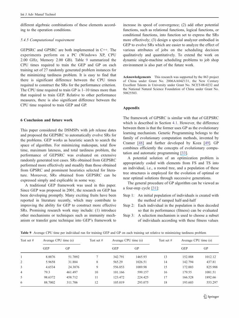
GEPSRC and GPSRC are both implemented in C++. Theexperiments perform on a PC (Windows XP, CPU2.00 GHz, Memory 2.00 GB). Table 9 summarized theCPU times required to train the GEP and GP on eachtraining set of 27 randomly generated problem instances forthe minimizing tardiness problem. It is easy to find thatthere is significant difference between the CPU timesrequired to construct the SRs for the performance criterion.The CPU time required to train GP is 1–10 times more thanthat required to train GEP. Relative to other performancemeasures, there is also significant difference between theCPU time required to train GEP and GP.

6 Conclusion and future work

This paper considered the DSMSPs with job release datesand proposed the GEPSRC to automatically evolve SRs forthe problems. GEP works as heuristic search to search thespace of algorithm. For minimizing makespan, total flowtime, maximum lateness, and total tardiness problem, theperformance of GEPSRC was evaluated on extensiverandomly generated test cases. SRs obtained from GEPSRCperformed more effectively and steadily than those obtainedfrom GPSRC and prominent heuristics selected for litera-ture. Moreover, SRs obtained from GEPSRC can beexpressed simply and explicable in some way.

A traditional GEP framework was used in this paper.Since GEP was proposed in 2001, the research on GEP hasbeen developing promptly. Many exciting fruits have beenreported in literature recently, which may contribute toimproving the ability for GEP to construct more effectiveSRs. Promising research work may include: (1) introduceother mechanisms or techniques such as immunity mech-anism or transfer gene technique into GEP’s framework to

increase its speed of convergence; (2) add other potentialfunctions, such as relational functions, logical functions, orconditional functions, into function set to express the SRsmore effectively; (3) design a special analyzer embodied inGEP to evolve SRs which are easier to analyze the effect ofvarious attributes of jobs on the scheduling decisionqualitatively and quantitatively. To extend the work ondynamic single-machine scheduling problems to job shopenvironment is also part of the future work.

Acknowledgements This research was supported by the 863 projectof China under Grant No. 2006AA04Z131, the New CenturyExcellent Talents in University under Grant No. NCET-08-0232 andthe National Natural Science Foundation of China under Grant No.50825503.

Appendix

The framework of GPSRC is similar with that of GEPSRCwhich is described in Section 4.1. However, the differencebetween them is that the former uses GP as the evolutionarylearning mechanism. Genetic Programming belongs to thefamily of evolutionary computation methods, invented byCramer [48] and further developed by Koza [49]. GPcombines efficiently the concepts of evolutionary compu-tation and automatic programming [33].

A potential solution of an optimization problem isappropriately coded with elements from FS and TS intoan individual, i.e., a rooted tree, and a population of thesetree structures is employed for the evolution of optimal ornear optimal solutions through successive generations.

The general procedure of GP algorithm can be viewed asa four-step cycle [31]:

Step 1: An initial population of individuals is created withthe method of ramped half-and-half

Step 2: Each individual in the population is then decodedso that its performance (fitness) can be evaluated

Step 3: A selection mechanism is used to choose a subsetof individuals according with these fitness values

Table 9 Average CPU time per individual run for training GEP and GP on each training set relative to minimizing tardiness problem

Test set # Average CPU time (s) Test set # Average CPU time (s) Test set # Average CPU time (s)

GEP GP GEP GP GEP GP

1 8.8876 51.7092 7 342.791 1465.93 13 152.888 1012.12

2 5.9658 31.884 8 565.29 1026.51 14 142.794 437.81

3 4.6534 24.3876 9 556.853 1089.98 15 172.003 825.988

4 79.3 461.497 10 101.166 599.157 16 179.55 1081.51

5 98.6372 458.712 11 123.472 224.425 17 166.528 1892.66

6 88.7002 311.706 12 105.019 293.075 18 193.603 553.297

Int J Adv Manuf Technol

Step 4: These individuals either survive intact to the newpopulation, or they are genetically modifiedthrough a number of operators. If the terminalcondition is satisfied, the procedure is finished,those individuals who perform the best (i.e., arethe most fit) are the solution of the optimizationproblem; otherwise, turn to Step 2.

Crossover and mutation are the two major operators thatare applied for the genetic modification of individuals.

Crossover Crossover begins by choosing two trees fromthe current population according to their fitness probabilis-tically. A sub-tree in each parent individual is selected atrandom. The randomly chosen sub-trees are then swapped,creating two new individual trees.

Mutation The mutation operation involves randomly select-ing a sub-tree within a parent individual that has beenselected from the population based on its fitness andreplacing it with a randomly generated sub-tree. Thegenerated sub-tree is created by randomly selecting ele-ments from FS and TS.

The brief descriptions serve only to provide backgroundinformation. For more detailed discussions of GP, thereader in encouraged to refer to [31, 48, 49].

References

1. Jakobovic D, Budin L (2006) Dynamic scheduling with geneticprogramming. Lect Notes Comput Sci 3905:73–84

2. Holthaus O, Rajendran C (1997) New dispatching rules forscheduling in a job shop - an experimental study. Int J Adv ManufTechnol 13(2):148–153

3. Kianfar K, Ghomi SMT, Karimi B (2009) New dispatching rulesto minimize rejection and tardiness costs in a dynamic flexibleflow shop. Int J Adv Manuf Technol 45(7–8):759–771

4. Wang JB, Wang LY, Wang D, Huang X, Wang XR (2009) A noteon single-machine total completion time problem with generaldeteriorating function. Int J Adv Manuf Technol 44(11–12):1213–1218

5. Ham M, Fowler JW (2008) Scheduling of wet etch and furnaceoperations with next arrival control heuristic. Int J Adv ManufTechnol 38(9–10):1006–1017

6. Norman B, Bean J (1999) A genetic algorithm methodology forcomplex scheduling problems. Nav Res Logist 46:199–211

7. Panneerselvam R (2006) Simple heuristic to minimize totaltardiness in a single machine scheduling problem. Int J AdvManuf Technol 30(7–8):722–726

8. Haupt R (1989) A survey of priority rule-based scheduling. ORSpektrum 11:3–16

9. Catoni O (1998) Solving scheduling problems by simulatedannealing. SIAM J Control Optim 36(5):1639–1675

10. Finke DA, Medeiros DJ, Traband MT (2002) Shop schedulingusing Tabu search and simulation. In: Yucesan E, Chen CH,Snowdon JL, Charnes JM (eds) Proceedings of the 2002 wintersimulation conference, 8–11 December 2002 San Diego. WSC,New York, pp 1013–1017

11. Goldberg DE (1989) Genetic algorithms in search, optimization,and machine learning. Addison–Wesley, Boston

12. Aytug H, Lawley MA, Mckay K, Mohan S, Uzsoy R (2005)Executing production schedules in the face of uncertainties: areview and some future directions. Eur J Oper Res 161(1):86–110

13. Graham RL (1966) Bounds for certain multiprocessor anomalies.Bell Syst Tech J 45:1563–1581

14. Smith WE (1956) Various optimizers for single-stage production.Nav Res Logist Q 3:59–66

15. Baker KR (1974) Introduction to sequencing and scheduling.Wiley, New York

16. Hoogeveen JA, Vestjens APA (1996) Optimal on-line algorithmsfor single-machine scheduling. Lect Notes Comput Sci 1084:404–414

17. Phillips C, Stein C, Wein J (1995) Minimizing average completiontime in the presence of release dates. Math Program 82:199–223

18. Kellerer H, Tautenhahn T, Woeginger GJ (1999) Approximabilityand nonapproximability results for minimizing total flow time ona single machine. SIAM J Comput 28(4):1155–1166

19. Guo Y, Lim A, Rodriguesc B, Yu S (2004) Minimizing total flowtime in single machine environment with release time: anexperimental analysis. Comput Ind Eng 47:123–140

20. Sgall J (1998) On-line scheduling. Lect Notes Comput Sci442:196–231

21. Pruhs K, Sgall J, Torng E (2004) Online scheduling. In: LeungJYT (ed) Handbook of scheduling: algorithms, models andperformance analysis. Chapman & Hall/CRC, Boca Raton

22. Blackstone JH, Phillips DT, Hogg GL (1982) A state-of-the-artsurvey of dispatching rules for manufacturing job shop operations.Int J Prod Res 20(1):27–45

23. Jeong KC, Kim YD (1998) A real-time scheduling mechanism fora flexible manufacturing system using simulation and dispatchingrules. Int J Prod Res 36(9):2609–2626

24. Yin YL, Rau H (2006) Dynamic selection of sequencing rules fora class-based unit-load automated storage and retrieval system. IntJ Adv Manuf Technol 29(11–12):1259–1266

25. Chen CC, Yih Y (1996) Identifying attributes for knowledge-basedevelopment in dynamic scheduling environments. Int J Prod Res34(6):1739–1755

26. El-Bouri A, Shah P (2006) A neural network for dispatching ruleselection in a job shop. Int J Adv Manuf Technol 31(3–4):342–349

27. Aytug H, Koehler GJ, Snowdon JL (1994) Genetic learning ofdynamic scheduling within a simulation environment. ComputOper Res 21(8):909–925

28. Trappey AJC, Lin GYP, Ku CC, Ho PS (2007) Design andanalysis of a rule-based knowledge system supporting intelligentdispatching and its application in the TFT-LCD industry. Int J AdvManuf Technol 35(3–4):385–393

29. Singh A, Mehta NK, Jain PK (2007) Multicriteria dynamicscheduling by swapping of dispatching rules. Int J Adv ManufTechnol 34(9–10):988–1007

30. Yang HB, Yan HS (2009) An adaptive approach to dynamicscheduling in knowledgeable manufacturing cell. Int J Adv ManufTechnol 42(3–4):312–320

31. Geiger CD, Uzsoy R, Aytug H (2006) Rapid modeling anddiscovery of priority dispatching rules: an autonomous learningapproach. J Sched 9:7–34

32. Koza JR (2007) Introduction to genetic programming. In: LipsonH (ed) Proceedings of GECCO 2007: genetic and evolutionarycomputation conference, 7-11 July 2007 London. ACM, London,pp 3323–3365

33. Dimopoulos C, Zalzala AMS (2001) Investigating the use ofgenetic programming for a classic one-machine schedulingproblem. Adv Eng Softw 32(6):489–498

Int J Adv Manuf Technol

34. Yin WJ, Liu M, Wu C (2003) Learning single-machine schedulingheuristics subject to machine breakdowns with genetic program-ming. In: Sarker R et al (eds) Proceeding of CEC2003: congresson evolutionary computation, 9-12 December 2003 Canberra,Australia. IEEE, Piscataway, pp 1050–1055

35. Atlan L, Bonnet J, Naillon M (1994) Learning distributed reactivestrategies by genetic programming for the general job shopproblem. In: Dankel D, Stewan J (eds) Proceedings of The 7thannual Florida artificial intelligence research symposium, 5-6 May1994 Pensacola Beach, Florida, USA. IEEE, Piscataway

36. Miyashita K (2000) Job-shop scheduling with genetic program-ming. In: Whitley LD, Goldberg DE et al (eds) Proceedings ofGenetic and Evolutionary Computation Conference (GECCO-2000), 8-12 July 2000 Las Vegas, Nevada, USA. Kaufmann, SanFrancisco, pp 505–512

37. Ho NB, Tay JC (2003) Evolving dispatching rules for solving theflexible job shop problem. In: Corne D (ed) Proceedings of the2005 IEEE congress on evolutionary computation, 2–4 September2005 Edinburgh, UK. IEEE, Piscataway, pp 2848–2855

38. Tay JC, Ho NB (2007) Designing dispatching rules to minimizetotal tardiness. Stud Comput Intel 49:101–124

39. Tay JC, Ho NB (2008) Evolving dispatching rules using geneticprogramming for solving multi-objective flexible job-shop prob-lem. Comput Ind Eng 54(3):453–473

40. Ferreira C (2001) Gene expression programming: a new adaptivealgorithm for solving problems. Complex Syst 13(2):87–129

41. Hardy Y, Steeb WH (2002) Gene expression programming andone-dimensional chaotic maps. Int J Mod Phys C 13(1):13–24

42. Jayamohan MS, Rajendran C (2000) New dispatching rules forshop scheduling: a step forward. Int J Prod Res 38:563–586

43. Montagne ER (1969) Sequencing with time delay costs. IndustrialEngineering Research Bulletin, Arizona State University 5

44. Oliver H, Chandrasekharan R (1997) Efficient dispatching rulesfor scheduling in a job shop. Int J Prod Econ 48(1):87–105

45. Kanet JJ, Li XM (2004) A weighted modified due date rule forsequencing to minimize weighted tardiness. J Sched 7(4):261–276

46. Bhaskaran K, Pinedo M (1992) Dispatching. In: Salvendy G (ed)Handbook of industrial engineering. Wiley, New York, pp 2184–2198

47. Vepsalainen APJ, Morton TE (1987) Priority rules for job shopswith weighted tardiness costs. Manage Sci 33:1035–1047

48. Cramer NL (1985) A representation for the adaptive generation ofsimple sequential programs. In: Grefenstette JJ (ed) Proceedingsof The First International Conference on Genetic Algorithms andtheir Applications, 24-26 July 1985 Pittsburgh, USA. Erlbaum,Hillsdale, pp 183–187

49. Koza JR (1994) Genetic programming II: automatic discovery ofreusable programs. MIT, Cambridge

Int J Adv Manuf Technol